CONSTANTIN ENEA, SUHA ORHUN MUTLUERGIL, GUSTAVO … · 1:2 Constantin Enea, Suha Orhun Mutluergil,...

1

Replication-Aware Linearizability

CONSTANTIN ENEA, University Paris Diderot, FranceSUHA ORHUN MUTLUERGIL, University Paris Diderot, FranceGUSTAVO PETRI, ARM Research, United KingdomCHAO WANG, University Paris Diderot, France

Geo-distributed systems often replicate data at multiple locations to achieve availability and performancedespite network partitions. These systems must accept updates at any replica and propagate these updatesasynchronously to every other replica. Conflict-Free Replicated Data Types (CRDTs) provide a principledapproach to the problem of ensuring that replicas are eventually consistent despite the asynchronous delivery ofupdates.

We address the problem of specifying and verifying CRDTs, introducing a new correctness criterion calledReplication-Aware Linearizability. This criterion is inspired by linearizability, the de-facto correctness criterionfor (shared-memory) concurrent data structures. We argue that this criterion is both simple to understand, and itfits most known implementations of CRDTs. We provide a proof methodology to show that a CRDT satisfiesreplication-aware linearizability which we apply on a wide range of implementations. Finally, we show that ourcriterion can be leveraged to reason modularly about the composition of CRDTs.

1 INTRODUCTIONConflict-Free Replicated Data Types (CRDTs) [Shapiro et al. 2011] have recently been proposedto address the problem of availability of a distributed application under network partitions. CRDTsrepresent a methodological attempt to alleviate the problem of retaining some data-Consistency andAvailability under network Partitions (CAP), famously known to be an impossible combination ofrequirements by the CAP theorem of Gilbert and Lynch [2002]. CRDTs are data types designedto favor availability over consistency by replicating the type instances across multiple nodes of anetwork, and allowing them to temporarily have different views. However, CRDTs guarantee that thedifferent states of the nodes will eventually converge to a state common to all nodes [Burckhardt2014; Shapiro et al. 2011]. This convergence property is intrinsic to the data type design and ingeneral no synchronization is needed, hence achieving availability.Availability vs. Consistency. To illustrate the problem we consider the implementation of a list-like CRDT object, the Replicated Growable Array (RGA) – due to Roh et al. [2011]1 –, used fortext-editing applications. RGA supports three operations: (1) addAfter(a,b) which adds thecharacter b – the concrete type is inconsequential here – immediately after the occurrence of thecharacter a assumed to be present in the list,2 (2) remove(a) which removes a assumed to bepresent in the list, and (3) read() which returns the list contents.

To make the system available under partitions, RGA allows each of the nodes to have a copy ofthe list instance. We will call each of the nodes holding a copy a replica. Then the question is, howcan we maintain the consistency of the different copies of the list given that the data could be at anypoint in time be modified or read by any of the replicas? A naive approach would synchronize all the

1We use a variation of code extracted from [Attiya et al. 2016].2We assume elements are unique, implemented with timestamps.

Authors’ addresses: Constantin Enea, University Paris Diderot, France, [email protected]; Suha Orhun Mutluergil, UniversityParis Diderot, France, [email protected]; Gustavo Petri, ARM Research, United Kingdom, [email protected]; ChaoWang, University Paris Diderot, France, [email protected].

2018. 2475-1421/2018/1-ART1 $15.00https://doi.org/

Proc. ACM Program. Lang., Vol. 1, No. CONF, Article 1. Publication date: January 2018.

arX

iv:1

903.

0656

0v1

[cs

.PL

] 1

5 M

ar 2

019

https://doi.org/

1:2 Constantin Enea, Suha Orhun Mutluergil, Gustavo Petri, and Chao Wang

replicas on each operation, hence maintaining coherence, but rendering the system unavailable if anyone replica goes off-line.

Instead, RGA allows any of the replicas to modify the local copy of the list immediately – andhence return control to the client – and lazily propagate the updates to the other replicas. For instance,assuming that we have an initial list containing the sequence a · b · e · f 3 and two replicas, r1 andr2, if r1 inserts the letter c after b (calling addAfter(b,c)), while r2 concurrently inserts theletter d after b (addAfter(b,d)) the replicas will have the states a · b · c · e · f and a · b · d · e · frespectively. We have solved the availability problem, but we have introduced inconsistent states.This problem is only exacerbated by adding more replicas.Convergence. To restore the replicas to a consistent state, CRDTs guarantee that under conflictingoperations – that is, operations that could lead to different states – there is a systematic way to detectconflicts, and there is a strategy followed by all replicas to deterministically resolve conflicts.

In the case of RGA, the implementation adds metadata to each item of the list identifying theoriginating replica as well as timestamp of the operation in that replica.4 This metadata is enough todetect when conflicts have occurred. Generally there are a number of assumptions that are necessaryfor the metadata to detect conflicts (for instance that timestamps increase monotonically with time)which we shall discuss in the following sections. Then, for RGA it is enough to know whethertwo addAfter operations have conflicted by simply comparing the replica identifiers and theirtimestamps. In fact, this is a sound over-approximation of conflict since two concurrent addAfteroperations have a real conflict only if their first arguments are the same (e.g. the element b in theexample aforementioned). In such case, the strategy to resolve the conflict will always choose toorder first the character added with the highest timestamp in the resulting list, and in the particularcase where the timestamps should be the same, an arbitrary order among replicas will be used. In theexample above, and assuming that the character c was added with timestamp t1 and the character dwas added with timestamp t2, if t2 < t1 (for some order ≤ between timestamps), the list will convergeto a · b · c · d · e · f. We obtain the same result if t1 = t2 and assume that we have a replica order<r , we have r2 <r r1. In any other case we obtain a · b · d · c · e · f. Using an arbitrary order amongreplica identifiers is common in CRDT implementations to break ties among elements with equaltimestamps. We will generally assume that metadata provides a strict ordering and ignore the details.

If the effects of all operations are delivered to all replicas eventually, the replicas will converge tothe same state – assuming a quiescent period of time where no new operations are performed. Thisallows to eventually recover the consistency of the data type without giving away availability.Specifications. The simplicity of the list data type with the API that we have described above allowsfor a somewhat simple conflict resolution strategy. Any strategy ordering conflicting concurrentinsertions in a deterministic way will work. However, this is not true for many other CRDT imple-mentations. It is therefore critical to provide the programmer with a clear, and precise, specificationof the allowed behaviors of the data type under conflicts. Unfortunately this is not an easy task. Manytimes the programmer has no option but to read the implementation to understand how the metadatais used to resolve conflicts, for instance by reading the algorithms by Shapiro et al. [2011] (a casewhere the algorithms are particularly well documented). Recently Burckhardt [2014]; Burckhardtet al. [2014] have developed a formal framework where CRDTs and other weakly consistent systemscan be specified. However, we consider that reading these specifications is far from trivial for theaverage programmer, let alone writing new specifications. Evidently, having a formal specification isa necessary step towards the verification of the implementations of CRDTs.

3We use s0 · s1 to denote the composition of sequences s0 and s1.4We ignore here conflicts due to remove. They are discussed in Sec. 2.


1:3

Simpler specifications, not simplistic specifications. It is important to remark at this point thatwhile it is our goal to make the specification of CRDTs simpler, we believe that it is impossibleto make them coincide with their sequential data type counterparts. Most CRDTs will exhibit,due to concurrency and consistency relaxations, behaviors that are not possible in the sequentialversion of the type they represent. A notable instance is the Multi-Valued-Register (MVR), whichresolves conflicts arising from concurrent updates to the register by storing multiple values. Hence,a subsequent read operation to the register might return a set of values rather than a single value.This is certainly a behavior that is not possible for a “traditional” register, and in fact, one that theprogrammer must be aware of. Our goal is to accurately specify the behaviors of the CRDT, meaningthat often times, different implementations of the same underlying data type (say a register) will havedifferent specifications if their conflict resolution allows for different behaviours, for instance theLast-Writer-Wins (LWW) and the MVR registers which will be mentioned later.Paper Contributions. Inspired by linearizability [Herlihy and Wing 1990] we propose a new consis-tency criterion for CRDTs, which we call Replication-Aware Linearizability (RA-linearizability).RA-linearizability both simplifies CRDT specifications, and allows us to give correctness proofstrategies for these specifications. To satisfy RA-linearizability a data type must be so that anyexecution of a client interacting with an instance of the data type (1) should result in a state that canbe obtained as a sequence (or linearization) of its updates – where we assume that all updates areexecuted sequentially– and (2) any operation reading the state of the data type instance should bejustified by executing a sub-sequence of the above mentioned sequence of updates. For instance, forthe RGA example, the state of the final list (when all updates are delivered) should be reachable byconsidering a sequence where all addAfter operations are executed sequentially. 5 This definitionshares some similarities with that of Perrin et al. [2014]. We address the main differences in Sec. 7.

Equipped with this criterion we show that many existing CRDTs are RA-linearizable. We provideboth, their specification, and proofs showing that implementations respect the specification. Weprovide two different proof methodologies based on the structure of the conflict-resolution mechanismimplemented by the CRDT. We categorize CRDT implementations into classes according to theirconflict-resolution strategy. Encouragingly, most of the CRDTs by Shapiro et al. [2011] can beproved RA-linearizable.

Given that our criterion is inspired by linearizability, we consider if it also preserves the samecompositionality properties, i.e. whether the composition of a set of RA-linearizable objects is alsoRA-linearizable. While we show that this is not true in general, we show that compositionality canbe achieved when we concentrate to specific classes of conflict resolution as described above.

Finally, we have mechanized our methodologies to prove RA-linearizability. We use the verificationtool Boogie [Barnett et al. 2005] to encode our specifications, CRDTs, and prove the correctnessof the implementations (proof scripts are available at [boo [n. d.]]). To the best of our knowledge,the only other works that mechanize correctness proofs of CRDT implementations are [Gomes et al.2017; Zeller et al. 2014], which are frameworks directly carrying the proofs at a semantical level inIsabelle/HOL, and concentrating on proving Strong Eventual Consistency (SEC).

Finally, notice that the CISE tool [Najafzadeh et al. 2016] does not actually prove the data types,but rather invariants on top of them.

2 OVERVIEWop(v)

r1 :

r2 :

r3 :

(origin)

Fig. 1. SystemModel.

We give an informal description of our system model, and illustrate ourcontribution with two compelling CRDT implementations from [Attiya et al.2016; Shapiro et al. 2011].

5We will come back to RGA to add remove in Sec. 2.



payload Ti-Tree N, Set Tombinitial N = ∅, Tomb = ∅addAfter(a,b) :generator :precondition : a = ◦ or (a != ◦ and (_,_,a) ∈ N and a < Tomb)let tb = getTimestamp()

effector(a, tb, b) :N = N ∪ {(a, tb, b)}

remove(a) :generator :precondition : (_,_,a) ∈ N and a < Tomb and a , ◦

effector(a) :Tomb = Tomb ∪ {a}

read() :let ret-list = traverse(N, Tomb)return ret-list

Listing 1. Replicated Growable Array (RGA) pseudo-code.

We assume that the system is comprised of multiple nodes in a network.We consider the implementation of CRDTs, and we focus on the behaviors ofan an instance of the data type, generically called an object. We assume thatobjects are replicated among several replicas. Fig. 1 shows the execution of an operation op(v)evolving as follows: (i) Firstly, a client issues a call to the object, connects to any one replica andperforms the operation in that replica. We call that replica the origin. (ii) If the operation readsand updates the object state, the reading action is only performed at the origin. This part of theoperation is called the generator (cf. [Shapiro et al. 2011]). Then, if the operation modifies the state –e.g. addAfter for RGA – an update is generated to be executed in every replica. This part of theoperation shall be called the effector. We assume that effectors are executed immediately at the origin.This is represented by the dot at the origin replica in Fig. 1. (iii) Finally, the effector is delivered toeach replica, and their states are updated consequently, represented by the target of the arrows. Thismodel corresponds to operation-based CRDTs. Our results also apply to state-based CRDTs, wherereplicas exchange states instead of operations (Sec. 6).

2.1 RGA CRDT ImplementationListing 1 presents the code of RGA in a style following that of Shapiro et al. [2011] (a version of theRGA introduced in [Attiya et al. 2016]).

The keyword payload declares the state used to represent the object: (akin to fields of a classin an object oriented language). a variable N of type Ti-Tree, and a variable Tomb of type Set.We then find the definitions of the operations: addAfter, remove and read. The effectfuloperations addAfter and remove have two labels marked in red: generator and effector,corresponding to the reading and updating part of the operations as described above. Notice that theeffector can use as arguments values produced by the generator. The precondition annotationindicates facts that are assumed about the state prior to the execution.

Reconsidering Fig. 1 the source of the arrows represents the execution of a generator jointlywith the effector at replica r1, and the target of the arrows represents the delivery and executionof the effector at replicas r2 and r3.

As it is common to many CRDT implementations, RGA replicas will use timestamps to keep trackof causality between updates, effectively capturing when two updates are concurrent. Moreover, theywill keep the information relating the causal order in which elements are added to the list. Providedwith this causality information – or lack thereof–, the timestamps will be used to resolve conflictsin a deterministic way. Each replica maintains a Timestamp Tree (Ti-Tree) containing in every


1:5

b : tb

a : ta

◦ : 0

c : tc

ta < tc < tb )a · b · c

T = ;

addAfter(c; d)

b : tb

a : ta

◦ : 0

ta < tc < tb <

a · b · c · ete < td )

T = fdgaddAfter(c; e)

c : tcb : tb

a : ta

◦ : 0

c : tc

ta < tc < tb <

a · b · c · d · e

e : ted : td

te < td )T = ;

b : tb

a : ta

◦ : 0

c : tc

ta < tc < tb <d : td

T = ;a · b · c · dtd )

remove(d)

e : ted : td

b : tb

a : ta

◦ : 0

c : tc

e : te

ta < tc < tb < a · b · c · eT = ;

te )

Fig. 2. Example of RGA conflict resolution.

tree node a pair with: the element added to the list (for instance the character b), and a timestampassociated to it (tb) used to resolve conflicts. We will encode the tree as a set of triples (correspondingto nodes) of the form (a, tb, b) representing an element b in the tree with timestamp tb and whoseparent is item a also present in the tree. The tree-ness property is ensured by construction.

The generator portion of addAfter(a,b) has a precondition requiring a to exist in the treebefore the insertion of b (the data structure is initialized with a preexisting element ◦). The generatorthen samples a timestamp tb for b which is assumed to be larger than any timestamp presently in theTi-Tree N of the origin replica.6 The effector portion of addAfter(a,b) adds the triple(a,tb,b) in the replica’s own copy of N. This ensures that the tree structure is consistent with thecausality of insertions in the data structure. A client of the object will only ever attempt to add anelement after another element which it has already seen as mandated by the addAfter API. Hence,the parent node of any node was inserted before it, and is causally related to it. Similarly, nodesthat are not related to each other on any path of the tree (eg. siblings) are not causally related. Anexample of such a tree is shown in the left most box of Fig. 2: elements c and b were concurrentlyadded after a, and a was added first after the initial element ◦.

From a Ti-tree, we can obtain a list by traversing the tree in pre-order, with the proviso thatsiblings are ordered according to their timestamps with the highest timestamp visited first. Theleftmost box in Fig. 2 shows a tree that results in the list a · b · c assuming the timestamp orderta < tc < tb.

Consider now two concurrent operations: addAfter(c,d) and addAfter(c,e) executingin two different replicas starting both with the state depicted on the left of Fig. 2. FollowingListing 1 we obtain the trees in the second column of Fig. 2 where we assume that the top tree isthe result of addAfter(c,d) in one of the replicas, and the bottom tree is the result of executingaddAfter(c,e) in the other. Then, the two trees result in different lists in each replica before theoperations are mutually propagated. In the third column of Fig. 2 we obtain the result of propagatingthe operations between the replicas – indeed the propagation of any of the operations to any of thereplicas yields the same result, ensured by the commutativity of CRDTs. It is clear now that the resultof the list is a · b · c · d · e.

We have so far ignored remove. Consider the case where a replica executes addAfter(a,b)on a replica while another one executes remove(a). If the effector of remove(a) reaches everyreplica after the effector of addAfter(a,b) there is no problem since the semantics is clear: theelement a is removed after the element b has been added. However, if the operations reach somereplica in opposite order (recall that they are concurrent) there is a problem since the preconditionof the effector of addAfter(a,b) requires that the element a be present in the Ti-tree of thereplica. To avoid this kind of conflict, rendering the operations commutative, RGA does not reallyremove elements from the Ti-tree. Instead, an additional data structure called a tombstone is used

6Also, tb cannot be sampled by another replica (as we discussed in Sec. 1 this can be ensured by tagging the timestamps withreplica identifiers).



addAfter(◦; a)addAfter(a; b)

addAfter(a; c)

remove(d)

addAfter(c; d)

addAfter(c; e)

Fig. 3. A history for the RGA object.

to keep track of elements that have been conceptually erased and should not be considered whenreading the list. Here, the marking of tombstones is a set Tomb of elements. The last column ofFig. 2 shows the result of a remove operation.

The method read performs the pre-order traversal explained before, where all elements in thetombstone Tomb are omitted. In each of the boxes of Fig. 2 the list shown represents the result of aread operation in the state depicted.

Operations, histories and linearizability. We consider an abstract view of executions of a CRDTobject called a history. Informally a history is a set of operations with a partial order representing theordering constraints imposed on the execution of each operation. We represent the execution of anoperation with a label of the form m(a) ⇒ b representing a call to method m with arguments a andreturning the value b. When the values are unimportant we shall use the meta-variable ℓ to denotea label. The partial order mentioned above represents the visibility relation among operations. Wesay that an operation with label ℓ1 is visible to an operation with label ℓ2 if at the time when ℓ2 wasexecuted at the origin replica, the effects of ℓ1 had been applied in the state of the replica executingℓ2. A history is a pair (L,≺) containing a set of labels L and a visibility relation ≺ between labels.The history of the execution in Fig. 2 is presented in Fig. 3. Each node represents a label and arrowsrepresent that the operation at the source of the arrow is visible to the operation at the target. Sincewe assume that visibility is transitive we ignore redundant arrows.

A similar notion of history is used in the context of linearizability [Herlihy and Wing 1990]. Theonly difference is that the order ≺ relates two operations the first of which returns before the otherone started. A history (L,≺) is called linearizable if there exists a sequential history (L,≺seq) (≺seq isa total order), called linearization, s.t. (L,≺seq) is a valid execution, and ≺ ⊆ ≺seq.

CRDTs are not linearizable since operations are propagated lazily, so two replicas can see non-coinciding sets of operations. We relax linearizability to adapt it to CRDTs as follows: (1) we requirethat the sequential history be consistent with the visibility relation among operations instead of thereturns-before order, and (2) operations that only read the state of the object are allowed to see asub-sequence of the linearization, instead of the whole prefix as in the case of linearizability. (Wewill discuss an additional relaxation in Sec. 2.2).Intuition of RGA RA-linearizability. To simplify, consider the linearization of two concurrent op-erations adding after a common element: addAfter(a,b) and addAfter(a,c). This examplecorresponds to the history shown in the first three nodes of Fig. 3 from left to right. Because theseoperations are concurrent they are not related by visibility so our criterion allows for any orderingamong them. Let us show that these operations can always be ordered in a way that the result offuture reads will match this ordering. From the previous explanation we know that the order betweenb and c in the resulting list will be determined by their corresponding timestamps (tb and tc).Assuming that the ordering is that given in the tree of the first column of Fig. 2, we know that we canorder the operations as addAfter(a,c) followed by addAfter(a,b) which when executedsequentially obviously results in a · b · c as shown. The timestamp metadata of RGA gives us astrategy to build the operation sequence that corresponds to a sequential specification. A concretelinearization of these operations is:


1:7

payload Set Sinitial S = ∅add(a) :generator :let k = getUniqueIdentifier()return k

effector(a, k) :S = S ∪ {(a, k)}

remove(a) :generator :let R = {(a,k) | (a,k) ∈ S}return R

effector(R) :S = S \ R

read() :let A = {a : ∃ k. (a,k) ∈ S}return A

Listing 2. Pseudo-code of the OR-Set CRDT.

addAfter(◦,a) · addAfter(a, c) · addAfter(a,b)Unfortunately this simple linearization strategy is not always applicable. Consider now a similar

case where after issuing the addAfter operations the replicas attempt to immediately read the state.As explained in Fig. 2, a possible behavior is that the first replica returns ◦ · a · b while the secondreturns ◦ · a · c. If we consider the linearization given above, the result ◦ · a · b is not possible, sincec was added before b was added. The problem here is that the replica executing this read has not yetseen the effect of addAfter(a, c). To overcome this problem we allow methods that read the state tosee a sub-sequence of the global linearization. Thus, we can consider the sequence

addAfter(◦,a) · addAfter(a, c) · read() ⇒ (◦ · a · c) ·addAfter(a,b) · read() ⇒ (◦ · a · b)

where the last read ignores the red label addAfter(a, c). These are only two cases of conflictingconcurrent operations, in Sec. 4 we show that all operations can be ordered such that they correspondto a sequential execution thereof.

2.2 OR-Set CRDT ImplementationThe Observed-Remove Set (OR-Set) [Shapiro et al. 2011] implements a set with operations: add(a),remove(a), read(). The code of OR-Set is shown in Listing 2 (we assume return values foradd(a) and remove(a) for technical reasons).

add(a)r1 :

r2 :add(a) remove(a)

Fig. 4. Interleaving-basedSet.

Although the meaning of these methods is self-evident from theirnames, the results of conflicting concurrent operations is not evident.Consider for example the case where two replicas add a certain ele-ment a and then one of them removes that element. If we consider aninterleaving based execution of these operations there are two optionsdepending on the interleaving: i) If remove(a) is the last operationthen the expected set is empty, since the two consecutive add(a) are idempotent, and the removewould remove the only occurrence of a. This interleaving is the one depicted with solid arrows inFig. 4. ii) On the other hand, if the operation add(a) of the non-removing process comes last, asdepicted with the dashed arrows in Fig. 4, the final set could contain the element a. As we haveexplained before, the operations can arrive in different orders to different replicas. To guaranteeconvergence, OR-Set must ensure that regardless of the ordering, the resulting set will be the same.To that end, OR-Set add operations will tag each added element with a unique identifier. Then, aremove operation will only remove the element-identifier pairs which has already seen. For instance,in the case (ii) above, the remove of a will only remove the element that has been previously added



add(b) ) 1r1 :

r2 :add(a) ) 3 add(b) ) 4

add(a) ) 2

remove(a) ) f(a; 3)g

remove(b) ) f(b; 1)g

fbg

fbgfag

fagfa; bg

fa; bg

fa; bg fa; bg

fa; bg fa; bg

read())fa; bg

read())fa; bg

(a) OR-Set non-linearizable execution. Each line represents operations issued tothe same replica.

add(b1)r1 :

r2 :add(a3) add(b4)

add(a2)

remove({a3})

remove({b1})

{b1}

{b1, b4}{a3}

{a2, a3}{a2, a3, b1}

{a3, b1, b4}

{a2, a3, b4} {a2, b4}

{a2, b1, b4} {a2, b4}

readIds(b)⇒{b1}

readIds(a)⇒{a3}

read()⇒{a, b}

read()⇒{a, b}

(b) Label rewriting of an OR-Set execution. Pairs (a,k) of an element a andidentifier k are written as ak .

Fig. 5. OR-Set Linearizability vs. RA-linearizability.

by the same replica, since this item has been observed by the remove operation – and thus itsidentifier is known to it. The concurrent add(a) operation will have an identifier that has not beenobserved by the remove Therefore the item will not be removed, even if the effectors of the twoadds are performed in a replica before the effector of the remove.Intuition of OR-Set Linearizability. It is easy to find examples where the implementation of OR-Set can produce executions that cannot be justified by the standard definition of linearizability (evenwith the relaxations discussed in Sec. 2.1) assuming a standard Set specification. Fig. 5a shows onesuch example. Clearly any linearization of the visibility relation in this execution should order theadd and remove updates before the read queries, and the linearization of the updates should endwith a remove. Therefore, the final set returned by each of the two read queries should have atmost one element (the read queries see all the updates in the execution), contrary to their returnvalue in this execution.

This execution shows that the remove operation behaves as both a query (observing a certainnumber of adds of the element to be removed) and an update (by removing said observed elements).To cope with such cases, we will consider in our definition that query-update operations can be splitinto a query part corresponding to the generator, which only reads the state – and hence is allowed tosee a sub-sequence of the linearization of updates – and an update part corresponding to the effectorwhich will use the results of the prior query. For instance, remove will be split into a query partreadIds where only the elements visible at the time of the remove are selected, and an updatepart remove where only those elements selected are erased. Any identifier not in the set returnedby readIds will remain in the set after the update part of remove. Evidently, this requires somemechanism for “marking” the adds that are concerned. We will consider that each add has a uniqueidentifier. Fig. 5b shows this rewriting. The result of the rewriting admits a linearization consistentwith the specification of Set, as explained above.

3 REPLICATION-AWARE LINEARIZABILITYIn this section we formalize the intuitions developed in Sec. 2. We define the semantics of CRDTobjects (§ 3.1), specifications (§ 3.2), and our notion of RA-linearizability (§ 3.3). For lack of space,our formalization focuses only on operation-based CRDTs. However, the notion of RA-linearizabilityapplies to state-based CRDTs as well (see Section 6).


1:9

3.1 The Semantics of CRDT objectsTo formalize the semantics of CRDT objects and our correctness criterion we use several semanticdomains summarized in Fig. 6. We let o ∈ O be a CRDT object in the set of objects O. Similarly,r ∈ R is a replica in the set of replicas R. We consider a set of method names m ∈ M, and that eachmethod has a number of arguments and a return value sampled from a data domain D. We assumethat the domain contains a special value ⊥ ∈ D used to represent the absence of a value (for instancethe return type of procedures). Furthermore, we ignore typing issues which should be addressedby an underlying programming language. Also, some methods, e.g., the method addAfter of theRGA object, generate timestamps from a totally-ordered domain T. We will use operation labels of

the form o.m(a)i,ts⇒ b to represent the call of a method m ∈ M of object o ∈ O, with argument a ∈ D,

resulting in the value b ∈ D, and generating the timestamp ts. Since there might be multiple callsto the same method with the same arguments and result, labels are tagged with a unique identifieri. We may omit the object o, the identifier i, the timestamp ts, or the return value b when they arenot important. The order relation on T is denoted by <. Abusing notations, we assume that the set Tcontains a distinguished minimal element ⊥ which we shall use for operations that do not generate

a timestamp such as the method remove of RGA. The timestamp ts of a label ℓ = o.m(a)i,ts⇒ b

is denoted ts(ℓ). We will ignore identifiers when unambiguous. The set of all operation labels isdenoted by L.

Given a CRDT object o, its semantics is defined as a labeled transition system (LTS) JoK =(GC,A, gc0,→), where GC is a set of global configurations, A is the set of transition labels calledactions, gc0 is the initial configuration, and→⊆ GC × A × GC is the transition relation. We use theaction genr(ℓ) to label the generator of ℓ when executed at replica r, and effr(ℓ) to label the effectorof ℓ when executed at r. For readability, we use gc

a−→ gc′ to denote a transition (gc,a, gc′) ∈→.Our semantics assumes the following two properties of the propagation of effectors: (i) the effector

of each operation is applied exactly once at each replica, and (ii) if the effector of operation ℓ1 isapplied at the origin replica of ℓ2 before ℓ2 happens, then for every replica r, the effector of ℓ2 willbe applied only after the effector of ℓ1 has already been applied. These are commonly referred to ascausal delivery. We assume causal delivery because our formalization focuses on operation-basedCRDTs. However, the notion of RA-linearizability and the compositionality results in Section 5apply to state-based CRDTs as well, even if the network infrastructure doesn’t satisfy causal delivery.

A global configuration (G, vis,DS) is a “snapshot” of the system that records all the operationsthat have been executed. G ∈ [R→ LC] 7 stores the local configuration of each replica (LC denotesthe set of local configurations). A local configuration (L,σ ) contains the state σ of a replica and theset L of labels of operations that originate at this replica, or whose effectors have been executed (orapplied) at this replica. When ℓ ∈ L, we say that ℓ is visible to the replica or that the replica seesℓ. The set of replica states σ is denoted by Σ. The relation vis ⊆ P(L × L) is the visibility relationbetween operations, i.e., (ℓ1, ℓ2) ∈ vis, where ℓ2 is an operation originated at a replica r, if the effectorof ℓ1 was executed at r before ℓ2 was executed. When (ℓ1, ℓ2) ∈ vis, we say that ℓ1 is visible to ℓ2, orthat ℓ2 sees ℓ1. As it will be clear from the definition of the transition relation, vis is a strict partialorder. Finally, DS ∈ [L → ∆] associates to each operation label ℓ ∈ L an effector δ ∈ [Σ → Σ],which is the replica state transformer generated when the operation was executed at the origin replica(∆ denotes the set of effectors). For some fixed initial replica state σ0, the initial global configurationis defined by gc0 = (G0, ∅, ∅) ∈ GC, where G0 maps each replica r into (∅,σ0).

The transition relation between global configurations is defined in Fig. 7. The first rule describes areplica r in state σ executing an invocation of method m with argument a. We use a function θ to

7We use [A→ B] to denote the set of total functions from A to B.



o ∈ O CRDT Objectsr ∈ R Replicasm ∈ M Methods

a,b ∈ D Datats ∈ T TimestampsL ⊆ L Label Set

ℓ ≡ o.m(a)i,ts⇒ b ∈ L Operation Label

Fig. 6. Semantic Domains.

OPERATION G(r) = (L, σ ) θ (σ , m, a) = (b, δ, ts) δ (σ ) = σ ′

ℓ = o.m(a)(i,ts )⇒ b unique(i) ts , ⊥ =⇒ (∀ℓ′ ∈ L. ts(ℓ′) < ts ) ∀ℓ′ ∈ labels(vis). ts(ℓ′) , ts

(G, vis, DS)genr(ℓ)−−−−−−→ (G[r← (L ∪ {ℓ }, σ ′)], vis ∪ (L × {ℓ }), DS[ℓ ← δ ])

EFFECTOR G(r) = (L, σ ) ℓ ∈ minvis(labels(vis) \ L) DS(ℓ) = δ δ (σ ) = σ ′

(G, vis, DS)effr(ℓ)−−−−−→ (G[r← (L ∪ {ℓ }, σ ′)], vis, DS)

Fig. 7. Operational Semantics of CRDTs. C[a ← b] denotes the in-place update of element a ofthe domain of C with value b; unique(i) to ensure that i is a unique identifier; and labels(vis) = {ℓ :∃ℓ′. (ℓ, ℓ′) ∈ vis ∨ (ℓ′, ℓ) ∈ vis}.represent the behavior of the generators of all methods collectively (the code under the generatorlabels), i.e., θ (σ ,m,a) stands for applying the generator of m with argument a on the replica state σ .Therefore, this transition applies the suitable generator, which results in a return value b, an effectorstate transformer δ to be applied on all replicas, and possibly, a timestamp ts. We have ts = ⊥for methods that don’t generate timestamps. We assume that timestamps are consistent with thevisibility relation vis, i.e., the timestamp ts generated by θ is strictly larger than all the timestamps ofoperations visible to r, and that each timestamp can be generated only once. The association betweenthe label ℓ corresponding to this invocation and the effector δ is recorded in the DS component ofthe new global configuration. We say that the effector δ is produced by the operation ℓ. The localconfiguration (L,σ ) of r is changed by applying the effector δ on the state σ , resulting in a new stateσ ′, and adding ℓ to the set of labels L. Finally, the visibility relation vis is changed to record thefact that the effectors of all operations in L have been applied before ℓ. This transition is labeled bygenr(ℓ) where ℓ is the label of this invocation. We may ignore the index r when it is not important.

The second rule describes a replica r in state σ executing the effector δ that corresponds to anoperation ℓ originated in a different replica. 8 The rule requires that δ is an effector of a label that hasnot yet been applied at r (i.e., its corresponding label is not in the L component of r’s configuration)and moreover, that it is a minimal one with respect to the order vis among such effectors, i.e., thereexists no ℓ′ < L such that (ℓ′, ℓ) ∈ vis. This transition results in modifying the state of r to δ (σ ) andadding ℓ to the set of operations whose effectors have been executed by r. Note that these transitionrules preserve the fact that vis is a strict partial order. This transition is labeled by effr(ℓ).

In what follows it will be useful to distinguish query (or pure) methods which do not modifythe state from state-modifying methods, which we shall call updates (or effectful). We say that amethod m ∈ M is a query if it always results (by applying the generator) in an identity effector δ(i.e. δ (σ ) = σ for all replica states σ ). We shall call an update any method m which is not a query –that is, whose effectors are not the identity function – and whose resulting effector and return valuedo not depend on the initial state σ of the origin replica. That is, its behavior is fully determinedby its arguments. More formally, assuming a functional equivalence relation ≡ between effectorsthat relates any two effectors that have the same effect (modulo the values of timestamps or uniqueidentifiers) m is called an update when θ (σ ,m,a)|2 ≡ θ (σ ′,m,a)|2, for every a ∈ D and two statesσ ,σ ′ ∈ Σ (for a tuple x , x |k denotes the projection of x on the k-th component). A method m which8This rule implies that we could simplify the first rule by not performing the effector immediately, but in general we assumeno interleavings of operations within a single replica.


1:11

is not a query nor an update is called a query-update. (It generates an effector which is not theidentity function, and whose effect depends on the local state of the replica at which the invocationof m originated.) For instance, the methods addAfter and remove of RGA, and add of OR-Set,are updates, the method remove of OR-Set is a query-update, and the read methods of both theRGA and the OR-Set are queries. We denote by Queries, Updates, and Query-Updates, the sets of

operation labels o.m(a)i,ts⇒ b where m is a query, an update, or query-update respectively. We shall

call them query, update, and query-update labels,respectively.An execution of the object o is a sequence of transitions gc0

a0−→ gc1a1−→ . . .. A trace tr is the

sequence of actions a0 · a1 . . . labeling the transitions of an execution. The set of traces of an object ois denoted by Tr(o). A history is a pair (L, vis) where vis ⊆ L × L is an acyclic relation over the set oflabels L. Given an execution e ending in a global configuration (G, vis,DS), the history of e, denotedby h(e), is the pair (labels(vis), vis). Note that the relation vis is a strict partial order in this case. Wewill later allow a more general notion of history in order to deal with object compositions (see Sec. 5).Also, the history of a trace tr, denoted by h(tr), is the history of the execution that corresponds to tr.The set of histories Hist(o) of an object o is the set of histories h of an execution e of o. A pictorialrepresentation of an execution (trace) can be found in Fig. 5a while an example of a history can befound in Fig. 3.

3.2 Sequential SpecificationsRA-linearizability provides an explanation for concurrent executions of CRDT objects in the form oflinearizations, which can be constrained using standard sequential specifications.

Definition 3.1 (Sequential Specification). A sequential specification (specification, for short) Specis a set of tuples (L, seq), where L is a set of labels and seq is a sequence including all the labels in L.

To describe sequential specifications in a succinct way we will provide an operational description.To that end, we will associate to specifications a notion of abstract state, which we shall generallydenote by ϕ and its domain shall be denoted by Φ. Then, to each valid label ℓ we will associate

a transition relation ϕℓ↪−→ ϕ ′ which, given an abstract state ϕ and provided that the label ℓ can be

applied in ϕ, produces a new abstract state ϕ ′. In the specific case where the label ℓ assumes a certainprecondition pre over the initial abstract state ϕ we will use Hoare-style preconditions and write(ϕ | pre(ϕ)

) ℓ↪−→ ϕ ′. In this way, a sequential specification is the set of labels that are accepted by the

successive application of the transition relation starting from some given initial state ϕ0.To illustrate the definition we provide the sequential specification of a very simple counter object,

as well as the RGA and OR-Set objects described before.

Example 3.2 (Sequential Specification of a Counter). In this case the state domain is Φ = Z, thatis the state will be an integer, and the transitions are given as follows:

kinc()⇒↪−−−−−→ k + 1 k

dec()⇒↪−−−−−−→ k − 1 k

read()⇒k↪−−−−−−−−→ k

Example 3.3 (Sequential Specification of RGA). Each abstract state ϕ = (l ,T ) contains a sequencel of elements of a given type and a set T of elements appearing in the list. The element l is the list ofall input values, whether already removed or not; while T stores the removed values and is used astombstone set. The sequential specification Spec(RGA) of list with add-after interface is defined by:(

(l1 · b · l2,T)| a fresh

) addAfter(b,a)↪−−−−−−−−−−−−→ (l1 · b · a · l2,T )(

(l ,T ) | b ∈ l and b , ◦) remove(b)

↪−−−−−−−−→ (l ,T ∪ {b})

(l ,T )read()⇒(l/T )↪−−−−−−−−−−−→ (l ,T )



where we denote by l/T the list resulting from removing all elements of T from l . The methodaddAfter(b,a) puts a immediately after b in l , assuming that each value is put into list at most once.Method remove(b) adds b into T , hence removing b from the list for subsequent calls to the readmethod. Finally read() ⇒ s returns the list content excluding any element appearing in T . Assumethat the initial value of list is (◦, ∅), and ◦ is never removed. We will sometimes ignore the value ◦from the return of read.

Example 3.4 (Sequential Specification of OR-Set). As explained in Fig. 5b, the fact that theOR-Set remove method is a query-update induces a rewriting of the operation labels in a history. Thisrewriting introduces update operations add(a, id), for some identifier id, instead of simply add(a),and remove(S), for some set S of pairs element-identifier, instead of remove(a), and a new queryoperation readIds(a) that returns a set of pairs element-identifier. These operations are specifiedas follows. The abstract state ϕ is a set of tuples (a, id), where a is a data and id is a identifier. Thesequential specification Spec(OR-Set) of OR-Set is given by the transitions:

ϕreadIds(a)⇒S↪−−−−−−−−−−−−→ ϕ [S = {(a, id) | (a, id) ∈ ϕ}]

ϕremove(S )↪−−−−−−−−→ ϕ \ S

( ϕ | (a, id) < ϕ )add(a, id)↪−−−−−−−→ ϕ ∪ {(a, id)}

ϕread(a)⇒A↪−−−−−−−−−→ ϕ [A = {a | ∃ id, (a, id) ∈ ϕ}]

Here readIds(a) ⇒ S returns the set of pairs with data a, remove(S) removes S from the abstractstate, add(a, id) puts {(a, id)} into the abstract state, and read() ⇒ A returns the value of the OR-Set.

This definition of specification of an object will be extended to a set of objects in Sec. 5. Anotherimportant aspect of specifications is whether they are deterministic or not. For instance the WookiCRDT [Weiss et al. 2007] is a list-like object that provides a method addBetween(a, b, c) whichinserts b between a and c. In contrast with RGA, where the method addAfter(a, b) adds the elementb immediately after a, in Wooki there are many possible positions where to insert b if a and c are notadjacent. In this case, to allow for any deterministic resolution mechanism our specifications shall benon-deterministic. This non-determinism in the specification has to be deterministically resolved bythe implementations to ensure convergence.

3.3 Definition of Replication-Aware LinearizabilityWe now provide the definition of RA-linearizability which characterizes histories of CRDT objects.To simplify the presentation, we consider first the case where all the labels in the history are eitherqueries or updates (query-updates are considered later). The intuition of RA-linearizability is thatthere is a global sequence (or linearization) of the update operations in an execution which canproduce the state of each replica when all the updates are visible to them. In intermediate steps, anyreplica state should be the result of applying a sub-sequence of updates of this global sequence. Thisis because replicas may see a subset of the updates performed up to some moment. Therefore, eachquery should be justified by considering the sub-sequence of the global sequence restricted to theupdates that are visible to that query. To be precise:

Definition 3.5. A history h = (L, vis) with L ⊆ Queries ⊎ Updates is RA-linearizable w.r.t. asequential specification Spec, if there exists a sequence (L, seq) – where we remark that the set oflabels are identical – such that:

(i) seq is consistent with vis, that is: vis ∪ seq is acyclic,(ii) the projection of seq to updates is admitted by Spec, i.e. seq↓Updates∈ Spec, where we denote

by seq ↓S the restriction of the order seq to the set S , and


1:13

(iii) for each query ℓqr ∈ L, the sub-sequence of updates visible to ℓqr together with ℓqr is itselfadmitted by Spec, i.e., seq↓vis−1(ℓqr)∩Updates · ℓqr ∈ Spec.

We say that (L, seq) is an RA-linearization of h w.r.t. Spec.

In a nutshell, this definition requires that for a given history, there exists a specification sequencesuch that (i) the set of labels are the same and the order in the sequence is consistent with the visibilityorder of the history, that (ii) when restricted to update operations – that is all the updates –, thesequence belongs to the specification, and that (iii) every query operation can be justified by thespecification based only on the updates that precede it in the sequence and that are visible to it. Withthis definition in mind it is not hard to check that the sequences of operations provided in Sec. 2.1and 2.2 are RA-linearizations. Another example constructing a linearization step by step is shownunder the label “timestamp-order linearizations” of Fig. 8.

We now consider the case where histories include query-updates. In such case, we apply Def-inition 3.5 on a rewriting of the original history where each query-update is decomposed into alabel representing the generator and another label representing the effector. As shown in Fig. 5bthis rewriting may introduce new labels of operations that have been added to the specification ofthe data type to provide specifications with no query-update operations. A mapping γ : L→ L≤2,where L≤2 is the set of labels and pairs of labels in L, is called a query-update rewriting. We assumethat every query or update label is mapped by γ to a singleton and that the γ image of such a labelpreserves its status, i.e., γ (ℓ) is a query, resp., update, whenever ℓ is a query, resp., update. Also,query-updates labels ℓ are mapped to pairs γ (ℓ) = (ℓ1, ℓ2) where ℓ1 is a query and ℓ2 is an update.These assumptions are important when applying Definition 3.5 on the rewriting of a history, sincethis definition relies on a partitioning of the labels into queries and updates. For a history h = (L, vis),its γ -rewriting is a history γ (h) = (L′, vis′) where• L′ is obtained by replacing each label ℓ in L with γ (ℓ) (a label may be replaced by two labels),• whenever a (query-update) label ℓ is mapped by γ to a pair (ℓ1, ℓ2), we have that the query is

ordered before the update, formally (ℓ1, ℓ2) ∈ vis′,• vis′ preserves the order between labels which are mapped to singletons, and for any query-

update label ℓ mapped to a pair (ℓ1, ℓ2), the query ℓ1 sees exactly the same set of operations asℓ and any operation which saw ℓ must see ℓ2. Formally, whenever (ℓ, ℓ′) ∈ vis we have that(upd(γ (ℓ)), qry(γ (ℓ′))) ∈ vis′, where for a label ℓ, qry(γ (ℓ)) (resp., upd(γ (ℓ))), is γ (ℓ) whenγ (ℓ) is a singleton, or its first (resp., second) component when γ (ℓ) is a pair.

Example 3.6 (Query-Update Rewriting of OR-Set). As shown in Fig. 5b, the query-update rewrit-ing for OR-Set is defined by: γ (add(a) ⇒ k) = add(a,k), γ (read() ⇒ A) = read() ⇒ A, andγ (remove(a) ⇒ R) = (readIds(a) ⇒ R, remove(R)).

The following extends Definition 3.5 to arbitrary histories using the rewriting defined above.

Definition 3.7 (Replication-Aware Linearizability). A history h = (L, vis) is RA-linearizablew.r.t. Spec, if there exists a query-update rewriting γ s.t. γ (h) is RA-linearizable w.r.t. Spec. AnRA-linearization w.r.t. Spec of γ (h) is called an RA-linearization w.r.t. Spec and γ of h.

A set H of histories is called RA-linearizable w.r.t. Spec when each h ∈ H is RA-linearizable w.r.t.Spec. A data type implementation is RA-linearizable w.r.t. Spec if for any object o of the data type,Hist(o) is linearizable w.r.t. Spec.

Reasoning with specifications. To illustrate the benefit of using RA-linearizability let us considera simple system where two replicas execute a sequence of operations on a shared OR-Set object:

add(a); rem(a); X = read() ∥ add(a); Y = read()



We are interested in checking that the following post-condition holds after the execution of theseoperations:

a ∈ X⇒ a ∈ YRewriting the program according to the specification of OR-Set discussed before, we obtain thefollowing, where the variable R represents the set of value timestamp pairs observed by the readIdsoperation as defined by the rewriting:

add(a, i1);readIds(a) ⇒ R;rem(R);X = read();{a ∈ X⇒ (a, i2) < R}

add(a, i2);Y = read();{(a, i2) < R⇒ a ∈ Y}

Post-condition : {a ∈ X⇒ a ∈ Y}

Since OR-Set is RA-linearizable w.r.t. the specification in Example 3.4 (proved in Section 4.1),the possible values of X and Y can be computed by enumerating their RA-linearizations. The post-condition follows from the conjunction of the assertions in each replica. Let us consider the validationof the assertion of right hand side with the following RA-linearization:

add(a, i2) add(a, i1) readIds(a) ⇒ R rem(R) Y = read()

We have in red color and with solid arrows the operations of the right hand side replica, and in bluewith dashed arrows the left ones. Let us consider the sub-sequence of the linearization that is visibleto the last operation (Y = read()). Since the first operation (add(a, i2)) is issued on the same replica,it must be visible to it. Let us now consider different cases for the operations of the other replica thatare visible to the read: (a) if the remove operation rem(R) is not visible to it, then the assertion istrivially true, because (a, i2) is in the resulting set according to the specification, and therefore theconsequent of the assertion is valid. Assume from now on that rem(R) is visible to it, there are twocases (b) if (a, i2) does not belong to R the consequent of the assertion is valid, since the addition of(a, i2) is necessarily visible to the read operation, and we conclude as before, (c) on the other hand, if(a, i2) ∈ R we have that the antecedent of the implication is falsified, and therefore the assertion isalso valid.

Here we have considered only one RA-linearization, but it is not hard to see that commuting theoperations of the different replicas renders the same argument. Importantly, this reasoning was doneentirely at the level of the RA-linearizations (i.e. the specification) of the data type.

For the assertion on the left hand side replica, since visibility includes the order between operationsissued on the same replica, we get that add(a, i1) is ordered before readIds(a) ⇒ R in every RA-linearization. Since add(a, i1) is also visible to readIds(a) ⇒ R, we get that (a, i1) ∈ R. Similarly,every RA-linearization will order rem(R) before the read() on the left replica, which implies that ifa ∈ X, then (a, i2) < R. Assuming the contrary, i.e., (a, i2) ∈ R, implies that R = {(a, i1), (a, i2)} andsince rem(R) is visible and linearized before X = read(), we get that a < X.

4 PROVING REPLICATION-AWARE LINEARIZABILITYWe describe a methodology for proving that CRDT objects are RA-linearizable which relies ontwo properties: (1) the effectors of any two concurrent operations (i.e., not visible to each other)commute, which is inherent to CRDT objects, and (2) the existence of a refinement mapping [Abadiand Lamport 1991; Lynch and Vaandrager 1995] showing that each effector produced by an operationℓ, respectively each query ℓ, is simulated by the execution of ℓ (or its counterpart through a query-update rewriting γ ) in the specification Spec. This methodology is used in two forms depending onhow the linearization is defined along an execution, which may affect the precise definition of therefinement mapping. We illustrate these two variations using OR-Set and RGA as examples.


1:15

4.1 Execution-Order LinearizationsWe first consider the case of CRDT objects, e.g., OR-Set, for which the order in which operationsare executed at the origin replica defines a valid RA-linearization. We say that such objects admitexecution-order linearizations. We start by formalizing the two properties we use to prove RA-linearizability.

Given a history h = (L, vis), we say that two operations ℓ1 and ℓ2 are concurrent, denoted ℓ1 ▷◁vis ℓ2,when (ℓ1, ℓ2) < vis and (ℓ2, ℓ1) < vis. In general, CRDTs implicitly require that the effectors ofconcurrent operations commute:

Commutativity: for every trace tr with h(tr) = (L, vis), and every two operations ℓ1, ℓ2 ∈ L, ifℓ1 ▷◁vis ℓ2, then

∀σ ∈ Σ. δℓ1 (δℓ2 (σ )) = δℓ2 (δℓ1 (σ ))

where δℓ1 and δℓ2 are the effectors of ℓ1 and resp., ℓ2.

Example 4.1. For OR-Set, two add, resp., remove, effectors commute because they both add,resp., remove, element-id pairs, while an add and a remove effector commute when they areconcurrent because the element-id pairs removed by the remove effector are different from the pairadded by the add effector (since the add is not visible to remove).

Commutativity implies that for every linearization lin of the operations in an execution, whichis consistent with the visibility relation, every replica state σ in that execution can be obtained byapplying the delivered effectors in the order defined by lin (between the operations corresponding tothose effectors). Indeed, by the causal delivery assumption, the order in which effectors are appliedat a given replica is also consistent with visibility. Therefore, the only differences between the orderin which effectors were applied to obtain σ in that execution and the linearization order lin involveeffectors of concurrent operations, which commute.

LEMMA 4.2. Let ρ be an execution of an object o satisfying Commutativity, h = (L, vis) thehistory of ρ, and (L, seq) a linearization of the operations in L (possibly, rewritten using a query-update rewriting γ ), consistent with vis. For each local configuration (Lr,σr) in ρ,

σr = δℓn (. . . (δℓ1 (σ0)) . . .)

where δℓ denotes the effector of operation ℓ, σ0 is the initial replica state, and seq ↓Lr= ℓ1 . . . ℓn .

In order to relate the CRDT object with its specification we use refinement mappings, which are“local” in the sense that they characterize the evolution of a single replica in isolation. A refinementmapping abs associates replica states with states of the specification, such that any update or queryapplied on a replica state σ can be mimicked by the corresponding operation in the specificationstarting from abs(σ ). Moreover, the resulting states in the two steps must be again related by abs.Formally, given a query-update rewriting γ , we define Refinement as the existence of a mapping abssuch that:

Simulating effectors: For every effector δ corresponding to a (query-)update operation ℓ, and everystate σ ∈ Σ,

σ ′ = δ (σ ) =⇒ abs(σ )upd(γ (ℓ))↪−−−−−−−→ abs(σ ′)

where ↪−→ is the transition function of Spec.Simulating generators: For every query m, and every σ ∈ Σ,

θ (σ ,m,a) = (b, _, _) =⇒ abs(σ ) ℓ↪−→ abs(σ )



where ℓ = m(a) ⇒ b. Recall that θ (σ ,m,a) stands for applying the generator of m withargument a on the state σ . Also, for every query-update m, and σ ∈ Σ,

θ (σ ,m,a) = (b, _, _) =⇒ abs(σ )qry(γ (ℓ))↪−−−−−−→ abs(σ ).

Example 4.3. Consider the OR-Set object, its specification in Example 3.4, and the query-updaterewriting in Example 3.6. Also, let abs be a refinement mapping defined as the identity function.The effector of an add(a) ⇒ k operation, rewritten by γ to add(a, k), and the add(a, k) operationof the specification have the same effect. Similarly, the effector of a query-update remove(a) ⇒ Roperation, rewritten by γ to (readIds(a) ⇒ R, remove(a, R)), and the remove(a, R) operation of thespecification have the same effect. Applying the query operation read() on a state σ results in thesame return value A as applying the same query in the context of the specification on the stateabs(σ ) = σ . Finally, for the query-update remove(a) ⇒ R, executing its generator in a state σ resultsin the same return value R as executing the query readIds(a) ⇒ R introduced by the query-updaterewriting in the specification state abs(σ ) = σ .

Next, we show that any object o satisfying Commutativity and Refinement is RA-linearizable.Given a history h = (L, vis) of a trace tr, the execution-order linearization of h is the sequence(γ (L), seq) such that γ (ℓ1) occurs before γ (ℓ2) in lin iff gen(ℓ1) occurs before gen(ℓ2) in tr, for everytwo labels ℓ1, ℓ2 ∈ L. An object o admits execution-order linearizations if for any history h = (L, vis)of a trace tr, the execution-order linearization is an RA-linearization of h w.r.t. Spec and γ .

THEOREM 4.4. Any object that satisfies Commutativity and Refinement admits execution-orderlinearizations.

PROOF. (Sketch) Clearly, any execution-order linearization is consistent with visibility. Then, wehave to argue that queries can be explained by applying the updates visible to them in linearizationorder (item (iii) in Definition 3.5). More precisely, we have to show that for each query ℓqr, thesequence seq′ · ℓqr where seq′ is the projection of seq on the set of updates visible to ℓqr is admittedby the specification. First, by Lemma 4.2, the state σ of the replica where ℓqr is applied is obtained byapplying the effectors of the operations visible to ℓqr in the linearization order. Then, by Refinement,every effector is simulated by the corresponding operation in the context of the specification. This

implies that abs(σ0)seq′↪−−→ abs(σ ), where σ0 is the initial replica state. The query ℓqr is also simulated

by the same operation in the context of the specification, which implies that abs(σ )ℓqr↪−→ abs(σ ).

These two facts imply that abs(σ0)seq′ ·ℓqr↪−−−−−→ abs(σ ) which means that seq′ · ℓqr is admitted by the

specification.Finally, the projection of seq on the updates is admitted by the specification since (1) any trace tr

can be extended with a query operation ℓ that sees all the (query-)updates in tr, and (2) the validity ofℓ w.r.t. the specification (shown above) implies in particular that the sequence of updates is admittedby the specification. □

We now discuss the issue of the non-deterministic specifications of Wooki, where an addBetween(a, b, c)operation inserts the element b at a random position between a and c (when a and c are not adjacent).The specification of the query read is however deterministic returning the whole list stored in thestate (excluding tombstone elements). Although the specification of these objects is non-deterministic,the proof of Lemma 4.2 and Refinement imply that the objects are convergent, in the sense that anytwo queries seeing the same set of updates return the same value. Indeed, by Lemma 4.2, the replicastates where such queries are applied are the same (assuming that effectors are deterministic, whichis the case in all the CRDTs we are aware of) and the existence of a refinement mapping implies


1:17

`2=addAfter(◦,b) tsb=⇒

r1 :

r2 :

`1=addAfter(◦,a) tsa=⇒ `3=addAfter(b,c)tsc=⇒

`4=read()⇒ b · a

execution-orderlinearizations:

timestamp-orderlinearizations :

`2 · `1`2 `2 · `1 · `3 `2 · `1 · `3 · `4

`1 · `2`2 `1 · `2 · `3 `1 · `2 · `4 · `3

Fig. 8. Execution-order and timestamp-order linearizations for RGA. Here tsa < tsb < tsc .

that the specification states corresponding to these replica states are also the same. The fact that thequeries are deterministic concludes the proof of convergence.

4.2 Timestamp-Order LinearizationsCRDT objects such as RGA in Listing 1, that use timestamps for conflict resolution, may notadmit execution-order linearizations. For instance, Fig. 8 shows an execution of RGA where tworeplicas r1 and r2 execute two addAfter invocations, and an addAfter invocation followed by aread invocation, respectively. An execution-order linearization which by definition, is consistentwith the order in which the operations are applied at the origin replica, will order addAfter(◦, b)before addAfter(◦, a). The result of applying these two operations in this order in the specificationSpec(RGA) (defined in Example 3.3) is the list a · b. However, if the timestamp tsa of a is smallerthan the timestamp tsb of b, a read that sees these two operations will return the list b · a, whichis different than the one obtained by applying the same operations in the context of Spec(RGA) inlinearization order. Such a sequence is not a valid RA-linearization (w.r.t. Spec(RGA)). Therefore,we consider a variation of the proof methodology described in Sec. 4.1 where the linearizations areadditionally consistent with the order of timestamps generated by the operations. We describe thisinstantiation using the RGA as an example (showing that it is RA-linearizable w.r.t. Spec(RGA)).More precisely, we consider linearizations where the operations that generate a timestamp, i.e.,addAfter, are ordered in the same order as their timestamps. For instance, in the execution of Fig. 8,addAfter(◦, a) will be ordered before addAfter(◦, b) because tsa is smaller than tsb (irrespectiveof the order between the generators). Moreover, to extend the notion of timestamp ordering tooperations ℓ that don’t generate timestamps, i.e., invocations of remove and read, we consider a“virtual” timestamp which is defined as the maximal timestamp of any operation visible to ℓ (or ⊥ ifno operation is visible to ℓ), and require that the linearization is consistent with the order betweenboth “real” 9 and “virtual” timestamps. For instance, the “virtual” timestamp of the read in Fig. 8 istsb because it sees addAfter(◦, a) and addAfter(◦, b). Then, a valid RA-linearization will order theread operation before the other addAfter(b, c) operation, since the timestamp tsc of the latter isbigger than the “virtual” timestamp tsb of the read. The operations that have the same timestamp(which is possible due to “virtual” timestamps) 10 are ordered as they execute at the origin replica.For instance, the read with “virtual” timestamp tsb is ordered after addAfter(◦, b) that has thesame timestamp tsb since it executes later at the origin replica.

Formally, for a history h = (L, vis), we define the timestamp tsh(ℓ) of a label ℓ in the context of thehistory h to be tsh(ℓ) = ts(ℓ) if ts(ℓ) , ⊥ and tsh(ℓ) = max {ts(ℓ′) : (ℓ′, ℓ) ∈ vis}, otherwise. Given ahistory h = (L, vis) of a trace tr, the timestamp-order linearization of h is the sequence (L, seq) suchthat γ (ℓ1) occurs before ℓ2 in lin iff tsh(ℓ1) < tsh(ℓ2) or gen(ℓ1) occurs before gen(ℓ2) in tr, for every

9That is, timestamps generated by the operation itself.10Among operations that have the same timestamp ts , there is exactly one operation generating ts , the rest of the operationshave ts as a “virtual” timestamp (i.e., they don’t generate timestamps and the maximal timestamp they see is ts).



two labels ℓ1, ℓ2 ∈ L. An object o admits timestamp-order linearizations if for any history h = (L, vis)of a trace tr, the timestamp-order linearization is an RA-linearization of h w.r.t. Spec. 11

Proving admittance of timestamp-order linearizations relies on Commutativity and a slight varia-tion of Refinement where intuitively, an effector generating a timestamp ts has to be simulated by aspecification operation only when it is applied on a state σ that doesn’t “store” a greater timestampthan ts (other effectors are treated as before). Formally, the set ts(σ ) of timestamps in a state σcontains all the timestamps ts generated by effectors applied to obtain σ . For RGA, the set of times-tamps in a state σ is the set of all timestamps stored in its timestamp tree. We define Refinementts bymodifying the “Simulating effectors” part of Refinement as follows:Simulating effectors: For every effector δ of an operation ℓ,

∀σ ∈ Σ. ts(ℓ) ≮ ts(σ ) ∧ σ ′ = δ (σ ) =⇒ abs(σ ) ℓ↪−→ abs(σ ′)

where ts(ℓ) ≮ ts(σ ) means that ts(ℓ) is not smaller than any timestamp in ts(σ ).

Example 4.5. Let us consider the RGA object, its specification in Example 3.3, and a refine-ment mapping abs which relates a replica state (N, Tomb) with a specification state (l ,T ) wherethe sequence l is given by the function traverse in read queries when ignoring tombstones, i.e.,l = traverse(N, ∅), and T = Tomb. It is obvious that remove effectors and read queries are sim-

ulated by the corresponding specification operations. Effectors of addAfter(a, b)tsb⇒ operations

are simulated by the specification operation addAfter(a, b) only when tsb is greater than all thetimestamps stored in the replica state where it applies. Thus, let (N, Tomb) be a replica state such that

ts < tsb for every ts with (_, ts, _) ∈ N. The result of applying the effector δ of addAfter(a, b)tsb⇒ is

to add b as a child of a. Then, applying traverse on the new state will result in a sequence whereb is placed just after a because it has the highest timestamp among the children of a. (and all thenodes in the tree N). This corresponds exactly to the sequence obtained by applying the operationaddAfter(a, b) in the context of the specification.

The proof of an object o admitting timestamp-order linearizations if it satisfies Commutativity andRefinementts is similar to the one of Theorem 4.4. Intuitively, although Refinementts is weaker thanRefinement, the fact that the timestamp-order linearizations are consistent with the order betweenthe timestamps generated by the operations, allows to show that any sequence of effectors consistentwith such a linearization can be simulated by a sequence of specification operations.

THEOREM 4.6. Any object that satisfies Commutativity and Refinementts admits timestamp-order linearizations.

We remark that the API of a CRDT can impact on whether it is RA-linearizable. For instance, aslight variation of the RGA in Listing 1 with the same state, but with an interface with a methodaddAt(a,k) to insert an element a at an index k, introduced in [Attiya et al. 2016], would not beRA-linearizable w.r.t. an appropriate sequential specification (see [Enea et al. 2019]).

5 COMPOSITIONALITY OF RA-LINEARIZABILITYWe investigate the issue of whether the composition of a set of objects satisfying RA-linearizability isalso RA-linearizable. While this is not true in general, we show that the composition of objects thatadmit execution-order or timestamp-order linearizations is RA-linearizable under the assumptionthat they share the same timestamp generator.

11For simplicity, we ignore query-update rewritings. The CRDTs with timestamp-order linearizations we investigated don’trequire such rewritings.


1:19

r1 :o1.add(d) o2.add(a)

r2 :

o2.add(b) o1.add(c)

Fig. 9. A history of two OR-Sets. Each operation is visible only at the origin, so visibility is given bythe horizontal lines.

5.1 Object Compositions and RA-LinearizabilityGiven two objects o1 and o2, the semantics of their composition o1 ⊗ o2 is the standard product ofthe LTSs corresponding to o1 and o2, respectively. Formally, given Jo1K = (GC1,A1, gc

10,→1) and

Jo2K = (GC2,A2, gc20,→2), we define Jo1 ⊗ o2K = (GC1 × GC2,A1 ∪ A2, (gc10, gc20, ∅),→1,2) where→1,2 = {((gc1, gc2),a1, (gc′1, gc2)) : (gc1,a1, gc′1) ∈→1}

∪ {((gc1, gc2),a2, (gc1, gc′2)) : (gc2,a2, gc′2) ∈→2}The history of a trace tr of o1 ⊗ o2 records a “global” visibility relation between the operationsin the trace, i.e., which operations of o1 or o2 are visible when issuing an operation of o1, andsimilarly, for operations of o2. Formally, h(tr) = (L, vis) where L is the set of labels occurring in tr,and (ℓ1, ℓ2) ∈ vis if there exists a replica r such that effr(ℓ1) occurs before genr(ℓ2) in the trace tr.In general, vis may not be a partial order since the causal delivery assumption holds only amongoperations of the same object. The set of histories Hist(o1 ⊗ o2) of the composition o1 ⊗ o2 is the setof histories h of a trace tr of o1 ⊗ o2.

For two specifications Spec1 and Spec2 of two objects o1 and o2, respectively, the compositionSpec1⊗Spec2 is the set of interleavings of sequences in Spec1 and Spec2, respectively. More precisely,Spec1 ⊗ Spec2 is the set of sequences (L, seq) such that their projection on labels of o1, resp., o2, isadmitted by Spec1, resp., Spec2. We say that the composition o1 ⊗ o2 is RA-linearizable if everyhistory of o1 ⊗ o2 is RA-linearizable w.r.t. Spec1 ⊗ Spec2. The extension to a set of objects is definedas usual.

Linearizability [Herlihy and Wing 1990] ensures that the composition of a set of linearizable ob-jects is also linearizable. More precisely, it ensures that for every history, any per-object linearizations,concerning the operations of a single object, can be combined into a global linearization, concern-ing all the operations in the history. By combining linearizations, we mean constructing a globallinearization whose projections on the operations of a single object are exactly the per-object lin-earizations considered in the beginning. However, this is not true for our notion of RA-linearizability.A counterexample is given in Fig. 9. The operations of o1 are represented using blank circles and theoperations of o2 using filled circles. The operations of o1 can be linearized to o1.add(c) · o1.add(d)(this is a valid RA-linearization since any sequence of add operations is admitted by Spec(OR-Set))while the operations of o2 can be linearized to o2.add(a) · o2.add(b). There is no RA-linearization ofthis history whose projections on each of the two objects correspond to these per-object lineariza-tions. Trying to construct a linearization where o2.add(a) occurs before o2.add(b) will imply thato1.add(d) must occur before o1.add(c) (since it must be consistent with the visibility relation), whichcontradicts the linearization of o1, and similarly for the other case, when trying to construct a globallinearization consistent with the linearization of o2’s operations. A reader knowledgeable of theliterature on linearizability may notice that this discrepancy between standard linearizability andRA-linearizability comes from the fact that the partial order defining a history in the case of standardlinearizability is actually an interval order12, while in the case of RA-linearizability it is an arbitrarypartial order.

12A partial order R is an interval-order if {(a, b), (c, d )} ⊆ R implies that (a, d ) ∈ R or (c, b) ∈ R, for every a, b, c, d .



5.2 Composition: Execution-Order LinearizabilityAlthough not all per-object RA-linearizations can be combined into global RA-linearizations, thismay still be true in some cases. For the history in Fig. 9, the operations of o1 can also be linearized too1.add(d) ·o1.add(c) which enables a global linearization o1.add(d) ·o2.add(a) ·o2.add(b) ·o1.add(c)whose projection on each object is consistent with the per-object linearization (we take the samelinearization o2.add(a) · o2.add(b) for o2).

The following theorem shows that in the case of RA-linearizable objects that admit execution-order linearizations, there always exist per-object RA-linearizations that can be combined into globalRA-linearizations, hence their composition is RA-linearizable and moreover, it also admits execution-order linearizations. A first preliminary result states that the order in which concurrent operations areexecuted at the origin replica can be permuted arbitrarily while still leading to a valid trace. Moreprecisely, for every linearization lin of the visibility in the history of a trace, there exists another validtrace where operations are executed at the origin replica in the order defined by lin.

LEMMA 5.1. Let tr be a trace of an object o and h(tr) = (L, vis). Then, for every sequence (L, lin)which is consistent with vis (i.e., vis ∪ lin is acyclic), there exists a trace tr ′ of o such that gen(ℓ1)occurs before gen(ℓ2) in tr ′ iff ℓ1 occurs before ℓ2 in lin. Moreover, tr ′ has the same history as tr.

PROOF. (Sketch) We define a dependency relation ⊚ between actions as follows: genr1 (ℓ1) ⊚effr2 (ℓ2) iff r1 = r2 or ℓ1 = ℓ2, genr1 (ℓ1)⊚genr2 (ℓ2) iff r1 = r2, effr1 (ℓ1)⊚genr2 (ℓ2) iff r1 = r2, andeffr1 (ℓ1)⊚effr2 (ℓ2) iff r1 = r2. Given a trace tr = tr1 ·a1 ·a2 ·tr2, we say that a trace tr ′ = tr1 ·a2 ·a1 ·tr2is derived from tr by a ⊚-valid swap iff a1 and a2 are not related by ⊚. Using standard reasoningabout traces of a concurrent system, it can be shown that if tr is a trace of o, then any trace tr ′ derivedthrough a sequence of ⊚-valid swaps is also a trace of o. Moreover, tr ′ has the same history as tr.Then, by the definition of the visibility relation vis in the history of a trace and the causal deliveryassumption, it can be shown that given a trace tr of o containing two actions gen(ℓ1) and gen(ℓ2)such that ℓ1 and ℓ2 are concurrent and gen(ℓ1) occurs before gen(ℓ2), there exists another trace tr ′ ofo that is defined through a sequence of ⊚-valid swaps, where gen(ℓ2) occurs before gen(ℓ1). Thus,the order of concurrent generator actions can be permuted arbitrarily, concluding the lemma. □

Lemma 5.1 implies that given an RA-linearizable object o, if it admits execution-order lineariza-tions, then every linearization of a history of o consistent with visibility is a valid RA-linearization.

LEMMA 5.2. Let o be an object which is RA-linearizable w.r.t. a specification Spec and admitsexecution-order linearizations. Then, for every history h = (L, vis) of o and every sequence (L, lin)which is consistent with vis, we have that (L, lin) is an RA-linearization of h w.r.t. Spec.

PROOF. (Skech) Let (L, lin) be a sequence consistent with the visibility relation ofh. By Lemma 5.1,there exists a trace tr of o such that gen(ℓ1) occurs before gen(ℓ2) in tr iff ℓ1 occurs before ℓ2 inlin. The definition of execution-order linearizations implies that (L, lin) is an RA-linearization ofh(tr) = h. □

Lemma 5.2 is the essential ingredient for proving that the composition of a set of RA-linearizableobjects that admit execution-order linearizations is also RA-linearizable. Intuitively, given a historyh with multiple such objects, any linearization of h is a valid RA-linearization since each of itsprojections on the set of operations of a single object is a linearization of the per-object visibilityrelation 13 and thus, a valid RA-linearization of that object.

THEOREM 5.3. The composition of a set of RA-linearizable objects that admit execution-orderlinearizations is RA-linearizable and admits execution-order linearizations.

13By definition, the visibility relation in the history of an object composition o1 ⊗ o2 projected on operations of o1, resp., o2,is exactly the visibility relation stored in the global configurations of o1, resp., o2 (at the end of the execution).


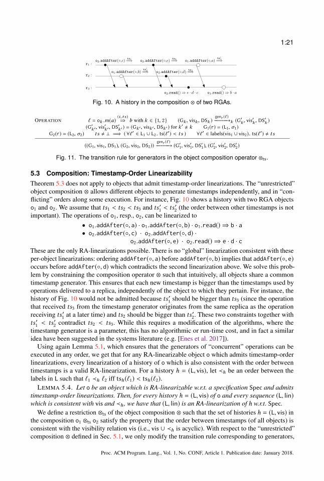
1:21

r1 :o2.addAfter(◦,c) ts1=⇒

r2 :o1.addAfter(◦,b)

ts′2=⇒

r3 :o2.read()⇒ e · d · c o1.read()⇒ b · a

o2.addAfter(◦,e) ts3=⇒ o1.addAfter(◦,a)ts′1=⇒

o2.addAfter(◦,d) ts2=⇒

Fig. 10. A history in the composition ⊗ of two RGAs.

OPERATION ℓ = ok .m(a)(i,ts )⇒ b with k ∈ {1, 2} (Gk , visk , DSk )

genr(ℓ)−−−−−−→k (G′k , vis′k , DS

′k )

(G′k′, vis′k′, DS

′k′ ) = (Gk′, visk′, DSk′ ) for k ′ , k G1(r) = (L1, σ1)

G2(r) = (L2, σ2) ts , ⊥ =⇒ (∀ℓ′ ∈ L1 ∪ L2 . ts(ℓ′) < ts ) ∀ℓ′ ∈ labels(vis1 ∪ vis2). ts(ℓ′) , ts((G1, vis1, DS1), (G2, vis2, DS2))

genr(ℓ)−−−−−−→ (G′1, vis′1, DS′1), (G′2, vis′2, DS′2)

Fig. 11. The transition rule for generators in the object composition operator ⊗ts.

5.3 Composition: Timestamp-Order LinearizabilityTheorem 5.3 does not apply to objects that admit timestamp-order linearizations. The “unrestricted”object composition ⊗ allows different objects to generate timestamps independently, and in “con-flicting” orders along some execution. For instance, Fig. 10 shows a history with two RGA objectso1 and o2. We assume that ts1 < ts2 < ts3 and ts ′1 < ts ′2 (the order between other timestamps is notimportant). The operations of o1, resp., o2, can be linearized to

• o1.addAfter(◦, a) · o1.addAfter(◦, b) · o1.read() ⇒ b · a• o2.addAfter(◦, c) · o2.addAfter(◦, d) ·

o2.addAfter(◦, e) · o2.read() ⇒ e · d · cThese are the only RA-linearizations possible. There is no “global” linearization consistent with theseper-object linearizations: ordering addAfter(◦, a) before addAfter(◦, b) implies that addAfter(◦, e)occurs before addAfter(◦, d) which contradicts the second linearization above. We solve this prob-lem by constraining the composition operator ⊗ such that intuitively, all objects share a commontimestamp generator. This ensures that each new timestamp is bigger than the timestamps used byoperations delivered to a replica, independently of the object to which they pertain. For instance, thehistory of Fig. 10 would not be admitted because ts ′1 should be bigger than ts3 (since the operationthat received ts3 from the timestamp generator originates from the same replica as the operationreceiving ts ′1 at a later time) and ts2 should be bigger than ts ′2. These two constraints together withts ′1 < ts ′2 contradict ts2 < ts3. While this requires a modification of the algorithms, where thetimestamp generator is a parameter, this has no algorithmic or run-time cost, and in fact a similaridea have been suggested in the systems literature (e.g. [Enes et al. 2017]).

Using again Lemma 5.1, which ensures that the generators of “concurrent” operations can beexecuted in any order, we get that for any RA-linearizable object o which admits timestamp-orderlinearizations, every linearization of a history of o which is also consistent with the order betweentimestamps is a valid RA-linearization. For a history h = (L, vis), let ≺h be an order between thelabels in L such that ℓ1 ≺h ℓ2 iff tsh(ℓ1) < tsh(ℓ2).

LEMMA 5.4. Let o be an object which is RA-linearizable w.r.t. a specification Spec and admitstimestamp-order linearizations. Then, for every history h = (L, vis) of o and every sequence (L, lin)which is consistent with vis and ≺h , we have that (L, lin) is an RA-linearization of h w.r.t. Spec.

We define a restriction ⊗ts of the object composition ⊗ such that the set of histories h = (L, vis) inthe composition o1 ⊗ts o2 satisfy the property that the order between timestamps (of all objects) isconsistent with the visibility relation vis (i.e., vis ∪ ≺h is acyclic). With respect to the “unrestricted”composition ⊗ defined in Sec. 5.1, we only modify the transition rule corresponding to generators,



as shown in Fig. 11. This ensures that a new generated timestamp is bigger than all the timestamps“visible” to the replica executing that generator (irrespectively of the object). Its extension to a setof objects is defined as usual. The composition operator ⊗ts is called shared timestamp generatorcomposition. Practically, if we were to consider the standard timestamp mechanism used in CRDTs,i.e., each replica maintains a counter which is increased monotonically with every new operation(originating at the replica or delivered from another replica) and timestamps are defined as pairs ofreplica identifiers and counter values, then ⊗ts can be implemented using a “shared” counter whichincreases monotonically with every new operation, independently of the object on which it is applied.

The following theorem shows that the composition of RA-linearizable objects that admit execution-order or timestamp-order linearizations is RA-linearizable, provided that all the objects share thesame timestamp generator.

THEOREM 5.5. The shared timestamp generator composition of a set of RA-linearizable objectsthat admit execution-order or timestamp-order linearizations is RA-linearizable.

The theorem above shows that any shared timestamp generator composition of the objects men-tioned in next section is RA-linearizable.

6 MECHANIZING RA-LINEARIZABILITY PROOFSTo validate our approach, we considered a range of CRDTs listed in Fig. 12 and mechanized theirRA-linearizability proofs using Boogie [Barnett et al. 2005], a verification tool. More precisely,we mechanized the proofs of conditions like Commutativity and Refinement which imply RA-linearizability by the results in Section 4. Beyond operation-based CRDTs (discussed in the paper),we have also considered state-based CRDTs, where an update occurs only at the origin, and replicasexchange their states instead of operations, and states from other replicas are merged at the replicareceiving them. The merge function corresponds to the least upper bound operator in a certain joinsemi-lattice defined over replica states.

For operation-based CRDTs, we have mechanized the proof of a strenghtening of Commutativitythat avoids reasoning about traces and the proof of Refinement (or Refinementts). ConcerningCommutativity, our proofs encode two effectors as a single procedure which executes on two equalcopies of the replica state. In some cases, the precondition of this procedure encodes conditionswhich are satisfied anytime the two effectors are concurrent, e.g., the effector of an add and resp.,remove of OR-Set are concurrent when the argument k of add is not in the argument R of remove.At least for the CRDTs we consider, such characterizations are obvious and apply generically toany conflict-resolution policy based on unique identifiers. In some cases, the effectors commuteeven if they are not concurrent, so no additional precondition is needed. We prove that the resultingstates are identical after performing the effectors in different order in each of the states. Refinement(or Refinementts) is reduced to proving that the refinement mapping is an inductive invariant for alock-step execution of the CRDT implementation and its specification.

For state-based CRDTs, we have identified a set of conditions similar to those of operation-basedCRDTs that imply RA-linearizability (see [Enea et al. 2019]). In this case, we don’t rely on thecausal delivery assumption. Extending their semantics with an auxiliary variable maintaining acorrespondence between replica states and sets of operations that produced them, we extract thevisibility relation between operations as in the case of operation-based CRDTs. This enables a similarreasoning about RA-linearizability. In particular, Commutativity is replaced by few conditions thatnow characterize the relationship between applying operations at a given replica and the mergefunction.


1:23

CRDT Imp. Lin.Counter [Shapiro et al. 2011] OB EOPN-Counter [Shapiro et al. 2011] SB EOLWW-Register [Johnson and Thomas 1975] OB TOMulti-Value Reg. [DeCandia et al. 2007] SB EOLWW-Element Set [Shapiro et al. 2011] SB TO

CRDT Imp. Lin.2P-Set [Shapiro et al. 2011] SB EOOR-Set [Shapiro et al. 2011] OB EORGA [Roh et al. 2011] OB TOWooki [Weiss et al. 2007] OB EO

Fig. 12. CRDTs proved RA-linearizable and the class of linearizations used. SB: State-Based, OB:Operation-Based, EO: Execution-Order, TO: Timestamp-Order.

7 RELATED WORKCorrectness Criteria. Burckhardt et al. [2014] gives the first formal framework where CRDTs andother weakly consistent replicated systems can be specified. Their CRDT specifications are definedin terms of sets of partial orders as opposed to our sequential specifications, which we think areeasier to reason about when verifying clients. Beyond simpler specifications, RA-linearizability isrelated to their formalization of causal consistency, called causal convergence in [Bouajjani et al.2017]. Overall RA-linearizability differs from causal convergence in three points: (1) query-updaterewritings, which enable sequential specifications and avoid partial orders, (2) the linearizationprojected on updates must be admitted by the specification (intuitively, this ensures that the "final"convergence state is valid w.r.t. the specification), and (3) the linearization is required to be consistentwith the visibility order from the execution, and not an arbitrary one as in causal convergence. Thelatter difference makes causal convergence not compositional.

Regarding convergence, RA-linearizability implies that there is a unique total order of updates,and therefore if at some point all updates are visible to all replicas, all subsequent query operationsat any replica will return the same value. This is observably equivalent to strong eventual consis-tency [Gomes et al. 2017; Shapiro et al. 2011; Zeller et al. 2014]. RA-linearizability is also strongerthan the session guarantees of Terry et al. [1994], but weaker than sequential consistency [Lamport1979] and linearizability [Herlihy and Wing 1990]. RA-linearizable objects that admit execution-order linearizations are close to being linearizable since the operations are linearized as they wereissued at the origin replica, relative to wall-clock time. This is similar to linearizability, where eachoperation appears to take effect instantaneously between the wall-clock time of its invocation itsresponse. Unlike linearizability, RA-linearizability allows queries to return a response consistentwith only a subsequence of its linearized-before operations.Sequential Specifications for CRDTs. Perrin et al. [2014] provides Update Consistency (UC), acriterion which to the best of our knowledge is the first to consider sequential specifications andcharacterize linear histories of operations. However UC is not compositional due to an existentialquantification over visibility relations like in causal convergence. Moreover, Perrin et al. [2014]doesn’t investigate UC proof methodologies.

Jagadeesan and Riely [2018] provide a correctness criterion called SEC, which differs fromRA-linearizability in several points: (1) Firstly, RA-linearizability has a global total order for updates,unlike SEC whose definition is quite complex. (2) Secondly, CRDT specifications in SEC areparameterized by a dependency relation at the level of the type’s API. Then, SEC assumes thatall independent operations commute and disregards their order even when issued by the sameclient. It is unclear how such a specification could adequately capture systems enforcing sessionguarantees [Terry et al. 1994]. RA-linearizability strives to preserve the guarantees of the underlyingsystem network since certain operations that appear independent at the API level could be madedata or control dependent by the client. This happens in our query-update rewritings where queriesprovide arguments for the subsequent update. (3) While SEC is also compositional, since operationsfrom different objects are assumed independent, a history of two different SEC objects is trivially



SEC since the order between operations of different objects is ignored. We find this notion ofcomposition problematic since the composition of specifications cannot capture causality betweendifferent objects, a common pattern when writing distributed applications (e.g. for referential integrityin a key-value store). In RA-linearizability the composition of a set of objects respects the client’scausality as illustrated by the failure to combine some per-object linearizations in Fig. 9. 14

Verification of CRDTs There are several works that approach the problem of verifying that a CRDTimplementation is correct w.r.t. a specification. In [Attiya et al. 2016; Burckhardt 2014; Burckhardtet al. 2014] along with the formal specification, proofs of correctness of implementations aregiven for several CRDTs. Our Refinement property is inspired by the Replication Aware Simulationsin [Burckhardt et al. 2014]. Compared to these simulations, our proofs remain at a much more abstractlevel – and are therefore simpler – since our specifications are simpler. We acknowledge however thattheir method is more general than ours which only applies to CRDTs satisfying RA-linearizability.Zeller et al. [2014] and Gomes et al. [2017] provide frameworks for the verification of CRDTs inIsabelle/HOL. Both works introduce a methodology to specify and prove CRDTs correct. Theirproofs are similar to the simulations of [Burckhardt et al. 2014], albeit in a different specificationlanguage also based on partial orders.

8 CONCLUSIONWe presented RA-linearizability, a correctness criterion inspired by linearizability, intended tosimplify the specification of CRDTs by resorting to sequential reasoning for the specifications. Weprovide proof methodologies for RA-linearizability for some well documented CRDTs, and we provethat under certain conditions these proofs guarantee the compositionality of RA-linearizability. In theextended version of this paper [Enea et al. 2019] we show how our techniques extend to state-basedCRDTs.

There are some limitations of RA-linearizability. Firstly, as we showed before, some CRDTsmight not be RA-linearizable under a certain API, but a slight change in the API renders themRA-linearizable. We would like to investigate what constitutes an API that enables RA-linearizabilityspecifications. secondly, while we argue that RA-linearizability simplifies specifications, we leave asfuture work to show whether it can be effectively used to verify client applications of a CRDT.

REFERENCES[n. d.]. https://github.com/menesro/RA-linearizability-proofsMartín Abadi and Leslie Lamport. 1991. The Existence of Refinement Mappings. Theor. Comput. Sci. 82, 2 (1991), 253–284.

https://doi.org/10.1016/0304-3975(91)90224-PHagit Attiya, Sebastian Burckhardt, Alexey Gotsman, Adam Morrison, Hongseok Yang, and Marek Zawirski. 2016. Specifica-

tion and Complexity of Collaborative Text Editing. In Proceedings of the 2016 ACM Symposium on Principles of DistributedComputing, PODC 2016, Chicago, IL, USA, July 25-28, 2016. 259–268. https://doi.org/10.1145/2933057.2933090

Michael Barnett, Bor-Yuh Evan Chang, Robert DeLine, Bart Jacobs, and K. Rustan M. Leino. 2005. Boogie: A ModularReusable Verifier for Object-Oriented Programs. In Formal Methods for Components and Objects, 4th InternationalSymposium, FMCO 2005, Amsterdam, The Netherlands, November 1-4, 2005, Revised Lectures. 364–387. https://doi.org/10.1007/11804192_17

Ahmed Bouajjani, Constantin Enea, Rachid Guerraoui, and Jad Hamza. 2017. On verifying causal consistency. In Proceedingsof the 44th ACM SIGPLAN Symposium on Principles of Programming Languages, POPL 2017, Paris, France, January 18-20, 2017, Giuseppe Castagna and Andrew D. Gordon (Eds.). ACM, 626–638. http://dl.acm.org/citation.cfm?id=3009888

Sebastian Burckhardt. 2014. Principles of Eventual Consistency. Foundations and Trends in Programming Languages 1, 1-2(2014), 1–150. https://doi.org/10.1561/2500000011

Sebastian Burckhardt, Alexey Gotsman, Hongseok Yang, and Marek Zawirski. 2014. Replicated data types: specification,verification, optimality. In The 41st Annual ACM SIGPLAN-SIGACT Symposium on Principles of Programming Languages,POPL ’14, San Diego, CA, USA, January 20-21, 2014. 271–284. https://doi.org/10.1145/2535838.2535848

14There are however per-object linearizations for this history which can be merged into a global linearization (see Sec. 5).


https://github.com/menesro/RA-linearizability-proofs

https://doi.org/10.1016/0304-3975(91)90224-P

https://doi.org/10.1145/2933057.2933090

https://doi.org/10.1007/11804192_17

https://doi.org/10.1007/11804192_17

http://dl.acm.org/citation.cfm?id=3009888

https://doi.org/10.1561/2500000011

https://doi.org/10.1145/2535838.2535848

1:25

Giuseppe DeCandia, Deniz Hastorun, Madan Jampani, Gunavardhan Kakulapati, Avinash Lakshman, Alex Pilchin, Swami-nathan Sivasubramanian, Peter Vosshall, and Werner Vogels. 2007. Dynamo: amazon’s highly available key-valuestore. In Proceedings of the 21st ACM Symposium on Operating Systems Principles 2007, SOSP 2007, Steven-son, Washington, USA, October 14-17, 2007, Thomas C. Bressoud and M. Frans Kaashoek (Eds.). ACM, 205–220.https://doi.org/10.1145/1294261.1294281

Constantin Enea, Suha Orhun Mutluergil, Gustavo Petri, and Chao Wang. 2019. Replication-Aware Linearizability. (2019).Vitor Enes, Paulo Sérgio Almeida, and Carlos Baquero. 2017. The Single-Writer Principle in CRDT Composition. In

Proceedings of the Programming Models and Languages for Distributed Computing (PMLDC ’17). ACM, New York, NY,USA, Article 4, 3 pages. https://doi.org/10.1145/3166089.3168733

Seth Gilbert and Nancy A. Lynch. 2002. Brewer’s conjecture and the feasibility of consistent, available, partition-tolerant webservices. SIGACT News 33, 2 (2002), 51–59. https://doi.org/10.1145/564585.564601

Victor B. F. Gomes, Martin Kleppmann, Dominic P. Mulligan, and Alastair R. Beresford. 2017. Verifying strong eventualconsistency in distributed systems. PACMPL 1, OOPSLA (2017), 109:1–109:28. https://doi.org/10.1145/3133933

Maurice Herlihy and Jeannette M. Wing. 1990. Linearizability: A Correctness Condition for Concurrent Objects. ACM Trans.Program. Lang. Syst. 12, 3 (1990), 463–492. https://doi.org/10.1145/78969.78972

Radha Jagadeesan and James Riely. 2018. Eventual Consistency for CRDTs. In Programming Languages and Systems -27th European Symposium on Programming, ESOP 2018, Held as Part of the European Joint Conferences on Theory andPractice of Software, ETAPS 2018, Thessaloniki, Greece, April 14-20, 2018, Proceedings. 968–995. https://doi.org/10.1007/978-3-319-89884-1_34

Paul R. Johnson and Robert Thomas. 1975. Maintenance of duplicate databases. RFC 677 (1975), 1–10. https://doi.org/10.17487/RFC0677

Leslie Lamport. 1979. How to Make a Multiprocessor Computer That Correctly Executes Multiprocess Programs. IEEETrans. Computers 28, 9 (1979), 690–691. https://doi.org/10.1109/TC.1979.1675439

Nancy A. Lynch and Frits W. Vaandrager. 1995. Forward and Backward Simulations: I. Untimed Systems. Inf. Comput. 121,2 (1995), 214–233. https://doi.org/10.1006/inco.1995.1134

Mahsa Najafzadeh, Alexey Gotsman, Hongseok Yang, Carla Ferreira, and Marc Shapiro. 2016. The CISE tool: provingweakly-consistent applications correct. In Proceedings of the 2nd Workshop on the Principles and Practice of Consistencyfor Distributed Data, PaPoC@EuroSys 2016, London, United Kingdom, April 18, 2016. 2:1–2:3. https://doi.org/10.1145/2911151.2911160

Gérald Oster, Pascal Urso, Pascal Molli, and Abdessamad Imine. 2006. Data consistency for P2P collaborative editing. InProceedings of the 2006 ACM Conference on Computer Supported Cooperative Work, CSCW 2006, Banff, Alberta, Canada,November 4-8, 2006, Pamela J. Hinds and David Martin (Eds.). ACM, 259–268. https://doi.org/10.1145/1180875.1180916

Matthieu Perrin, Achour Mostéfaoui, and Claude Jard. 2014. Update Consistency in Partitionable Systems. In DistributedComputing - 28th International Symposium, DISC 2014, Austin, TX, USA, October 12-15, 2014. Proceedings. 546–549.http://link.springer.com/content/pdf/bbm%3A978-3-662-45174-8%2F1.pdf

Hyun-Gul Roh, Myeongjae Jeon, Jinsoo Kim, and Joonwon Lee. 2011. Replicated abstract data types: Building blocks forcollaborative applications. J. Parallel Distrib. Comput. 71, 3 (2011), 354–368. https://doi.org/10.1016/j.jpdc.2010.12.006

Marc Shapiro, Nuno Preguiça, Carlos Baquero, and Marek Zawirski. 2011. A comprehensive study of Convergent andCommutative Replicated Data Types. Research Report RR-7506. Inria – Centre Paris-Rocquencourt ; INRIA. 50 pages.https://hal.inria.fr/inria-00555588

Douglas B. Terry, Alan J. Demers, Karin Petersen, Mike Spreitzer, Marvin Theimer, and Brent B. Welch. 1994. SessionGuarantees for Weakly Consistent Replicated Data. In Proceedings of the Third International Conference on Parallel andDistributed Information Systems (PDIS 94), Austin, Texas, USA, September 28-30, 1994. IEEE Computer Society, 140–149.https://doi.org/10.1109/PDIS.1994.331722

Stéphane Weiss, Pascal Urso, and Pascal Molli. 2007. Wooki: A P2P Wiki-Based Collaborative Writing Tool. In WebInformation Systems Engineering - WISE 2007, 8th International Conference on Web Information Systems Engineering,Nancy, France, December 3-7, 2007, Proceedings (Lecture Notes in Computer Science), Boualem Benatallah, Fabio Casati,Dimitrios Georgakopoulos, Claudio Bartolini, Wasim Sadiq, and Claude Godart (Eds.), Vol. 4831. Springer, 503–512.https://doi.org/10.1007/978-3-540-76993-4_42

Peter Zeller, Annette Bieniusa, and Arnd Poetzsch-Heffter. 2014. Formal Specification and Verification of CRDTs. In FormalTechniques for Distributed Objects, Components, and Systems - 34th IFIP WG 6.1 International Conference, FORTE 2014,Held as Part of the 9th International Federated Conference on Distributed Computing Techniques, DisCoTec 2014, Berlin,Germany, June 3-5, 2014. Proceedings. 33–48. https://doi.org/10.1007/978-3-662-43613-4_3


https://doi.org/10.1145/1294261.1294281

https://doi.org/10.1145/3166089.3168733

https://doi.org/10.1145/564585.564601

https://doi.org/10.1145/3133933

https://doi.org/10.1145/78969.78972

https://doi.org/10.1007/978-3-319-89884-1_34

https://doi.org/10.1007/978-3-319-89884-1_34

https://doi.org/10.17487/RFC0677

https://doi.org/10.17487/RFC0677

https://doi.org/10.1109/TC.1979.1675439

https://doi.org/10.1006/inco.1995.1134

https://doi.org/10.1145/2911151.2911160

https://doi.org/10.1145/2911151.2911160

https://doi.org/10.1145/1180875.1180916

http://link.springer.com/content/pdf/bbm%3A978-3-662-45174-8%2F1.pdf

https://doi.org/10.1016/j.jpdc.2010.12.006

https://hal.inria.fr/inria-00555588

https://doi.org/10.1109/PDIS.1994.331722

https://doi.org/10.1007/978-3-540-76993-4_42

https://doi.org/10.1007/978-3-662-43613-4_3


r1 :

r2 :addAfter(◦, b)

addAfter(◦, a) addAfter(b, c)

addAfter(b, d)

G(r1).L =

addAfter(◦, a),addAfter(◦, b),addAfter(b, c)

G(r1).Tomb = ∅G(r1).N :

b : tsb a : tsa

c : tsc(addAfter(◦, a), addAfter(b, c)),(addAfter(◦, b), addAfter(b, c)),(addAfter(◦, b), addAfter(b, d))

G.vis =

(a)

r1 :



addAfter(b, d)

G(r1).L =

addAfter(◦, a),addAfter(◦, b),addAfter(b, c),addAfter(b, d)

G(r1).Tomb = ∅G(r1).N :

b : tsb a : tsa

c : tscd : tsd(addAfter(◦, a), addAfter(b, c)),(addAfter(◦, b), addAfter(b, c)),(addAfter(◦, b), addAfter(b, d))

G.vis =

(b)

r1 :



addAfter(b, d)

G(r1).L =

addAfter(◦, a),addAfter(◦, b),addAfter(b, c),addAfter(b, d)remove(b)

G(r1).Tomb = {b}G(r1).N :

b : tsb a : tsa

c : tscd : tsd

(addAfter(◦, a), addAfter(b, c)),(addAfter(◦, b), addAfter(b, c)),(addAfter(◦, b), addAfter(b, d)),(addAfter(◦, a), remove(b)),(addAfter(b, c), remove(b)),(addAfter(◦, a), remove(b)),(addAfter(b, d), remove(b))

G.vis =

remove(b)

(c)

Fig. 13. Example of the semantics of RGA.

A TRANSITION RULES OF THE CRDT SEMANTICSFig. 13 shows how some components of the semantics progress according to the rules of Fig. 7 for theRGA data type. In particular we shown: the local labels of replica r1 (G(r1).L); its state, where weremove the σ for succinctness (then G(r1).σ .N becomes G(r1).N); and the global visibility relationG.vis. The transition from Fig. 13b to Fig. 13c shows an transition where the operation remove(b)is executed by replica r1. Notice in particular how the global visibility relation is extended.

In Fig. 13, the transition from Fig. 13a to Fig. 13b corresponds to a transition which extends thevisibility of the operation addAfter(b, d) to r1. Notice that this is reflected in the G(r1).L component.The relation G.vis does not change since this relation only changes when a new operation is executedat the source replica.

B IMPLEMENTATIONS OF OPERATION-BASED CRDT AND THEIR SEQUENTIALSPECIFICATIONS

B.1 Operation-Based Counter and Its Sequential SpecificationImplementation: The operation-based counter of [Shapiro et al. 2011] is shown in Listing 3. Itimplements a counter interface with operations: inc(), dec() and read. A payload is a integer ctr .inc increase the counter value of replica state by 1, dec decrease the counter value of replica stateby 1, and read returns the counter value of replica state.Sequential Specification Spec(Counter): Each abstract state ϕ is a integer. The sequential specifi-cation Spec(Counter) of counter is defined by:


1:27

payload integer ctrinitial ctr = 0

inc() :generator :effector(inc) :ctr = ctr + 1

dec() :generator :effector(dec) :ctr = ctr - 1

read() :return ctr

Listing 3. Pseudo-code of operation-based counter

ϕinc()↪−−−→ ϕ + 1

ϕdec()↪−−−→ ϕ − 1

ϕread()⇒ϕ↪−−−−−−−→ ϕ

Method inc() increase the counter value by 1. Method dec() decrease the counter value by 1.Method read() ⇒ k returns the counter value.

B.2 Operation-Based Last-Writer-Win Register and its Sequential SpecificationImplementation: The operation-based last-writer-win Register (LWW-Register) of [Shapiro et al.2011] is shown in Listing 4. It implements a register interface with operations: write(a) and read.A payload is a tuple (x , ts) of a data value x and its timestamp ts. Here x0 is an initial data and ts0 isan initial timestamp.

write(a) generates a new timestamp ts ′ and modifies the replica state into (a, ts ′), and its effectoruses the argument (a, ts ′). When applying an effector with arguments (a, ts ′) from a replica (b, tsb ),the resulting replica state is (a, ts ′) if tsb < ts ′, and is (b, tsb ) otherwise. read returns the data valueof replica state.Sequential Specification Spec(Reg): Each abstract state ϕ is a data value. The sequential specifica-tion Spec(Reg) of LWW-register is defined by:

ϕwrite(a)↪−−−−−−→ a

ϕread()⇒ϕ↪−−−−−−−→ ϕ

Method write(a) update the abstract state into data value a. Method read() ⇒ ϕ returns the valueof the register.



payload X x, timestamp tsinitial x0, ts0

write(a) :generator :let ts ′ = getTimestamp()

effector((a,ts ′)) :if (ts < ts ′)(x,ts) = (a,ts ′)

read() :return x

Listing 4. Pseudo-code of operation-based LWW-register

B.3 Operation-Based Wooki and its Sequential SpecificationImplementation: The Wooki implementation of [Weiss et al. 2007] is given in Listing 5. Wooki isan optimized version of Woot [Oster et al. 2006]. To make our introduction more clear, we borrowthe notion of W-character and W-string from Woot.

Wooki implements a list interface with operations: addBetween(a,b, c), remove(a) and read. Apayload is a W-string (introduced below) strinдs which stores the information of list content as wellas tombstone.

A W-character w is a tuple (id,v,deдree, f laд), and is used to stroe the information of an elementof list. Here id is the identifier ofw;v is the value ofw; deдree is the degree ofw; f laд ∈ {true, false}is the flag of w and indicates whether w is “visible” in list. A identifier id of W-character is a uniquetimestamp. We use deдree(w) to denote the degree of w . A degree is a integer that is fixed when itsW-character is generated; when inserting an W-character into strinдs , the degree of W-characters ofstrinдs influenced the position where this W-character will be inserted into.

Let ◦beдin and ◦end be two special values. Letwbeдin = (_, ◦beдin , 0, true) andwend = (_, ◦end , true)be two special W-characters. A W-string is an ordered sequence of W-characters wbeдin ·w1 · . . . ·wn ·wend . We never remove ◦beдin or ◦end , and never put value before ◦beдin or after ◦end . Sincewbeдin and wend is fixed to be the head and tail of a W-string, in the latter part of this paper, when weconsidering the content of a W-string, we ignore wbeдin and wend . We define the following functionsfor a W-string str :

- |str | returns the length of str ,- str [p] returns the W-character at position p in str . Here we assume that the first element of str

is at position 0.- pos(str ,w) returns the position of W-character w in str .- insert(str ,w,p) inserts W-character w into str at position p.- subseq(str ,w1,w2) returns the part of str between the W-characters w1 and w2 (excluding w1

and w2).- contains(str ,a) returns true if there exists a W-character in str with value a.- values(str ) returns the sequence of visible (with true flag) values of str .- getWchar(str ,a) returns the W-character with value a in str .- changeFlag(str ,pos, f ) changes the flag of str [pos] into boolean value f .


1:29

payload W-string strinдsinitial strinдs = ϵ

addBetween(a,b,c) :generator :precondition : c , ◦beдin ∧ a , ◦end ∧ b , ◦beдin ∧ b , ◦end ∧

contains(strinдs ,a) ∧ contains(strinдs , c) ∧ pos(strinдs , c) > pos(strinдs ,a) ∧¬contains(strinдs ,b)

let ts = getTimestamp()let wp = дetWchar (strinдs ,a)let wn = дetWchar (strinдs , c)

effector((w,wp,wn)) : with w = (ts,b,max(deдree(wp ),deдree(wn)) + 1, true)integrateIns(wp ,w,wn)

remove(a) :generator :precondition : a , ◦beдin ∧ a , ◦end ∧ contains(strinдs ,a)let w = дetWchar (strinдs ,a)

effector(w) :let p = pos(strinдs ,w)chanдeFlaд(strinдs ,p, false)

read() :let s = values(strinдs )return s

integrateIns(wp ,w,wn)let S = strinдslet S ′ = subseq(S,wp ,wn)if S ′ = ϵthen insert(S,w,pos(S,wn))

elseLet i = 0Let dmin be the minimal degree of W-characters in S ′

Let F be projection of S ′ into W-characters with degree dminif (w <id F [0])integrateIns(wp ,w, F [0])

elsewhile (i < |F | − 1 ∧ F [i] <id w) do

i = i+1if (i = |F | − 1 ∧ F [i] <id w)

integrateIns(F [i],w,wn)else

integrateIns(F [i − 1],w, F [i])Listing 5. Pseudo-code of Wooki



A total order <id is given for identifiers of W-characters for conflict resolution, and let <id be thetotal order of timestamps (identifiers of W-charcaters). Given a W-string str and two W-charactersw1,w2 of str , we write w1 <str w2 to indicate that pos(str ,w1) < pos(str ,w2).

Note that, here we use addBetween method, which “adds a value between two values”, and isdifferent from the addAfter method of RGA. Also, note that a value can be inserted into the listonly once.

addBetween(a,b, c) intends to generate a new W-character w with value b and put it betweenW-characters with values a and c,respectively. addBetween(a,b, c) work as follows: First, wecheck the precondition, such as three exists W-characters with values a and c in strinдs , andthe W-character with value a is before the W-character with value c in strinдs . Then, let wpand wn be the W-characters with value a and c in strinдs , respectively, and we generate a W-character w = (ts,b,max(deдree(wp ),deдree(wn)) + 1, true) with value b. Finally, we call methodinteдrateIns(wp ,w,wn) to put w into strinдs at some position between wp and wn .inteдrateIns(wp ,w,wn) is a recursive method and works as follows: If there are no W-character

between wp and wn , then w is put after wp . Else, Wooki selects a sequence F of W-characters, suchthat each W-character of F is between wp and wn , and has minimal degree. Then, we choose theposition of w according to <id order, and recursive call inteдrateIns(wx ,w,wy ) for some wx ,wy ∈F ∪ {wp ,wn}. We can see that, the minimal degree of W-characters of subseq(S,wx ,wy ) is largerthan that of subseq(S,wp ,wn), and subseq(S,wx ,wy ) is a sub-sequence of subseq(S,wp ,wn).

remove(a) first finds the W-character with value a in strinдs and then sets its flag into false. readuses values(strinдs ) to return the list content of strinдs .Sequential Specification Spec(Wooki): Each abstract state ϕ = (l ,T ) contains a sequence l ofelements of a given type and a set T of elements appearing in the list. The element l is the list ofall input values, whether already removed or not; while T stores the removed values and is used astombstone. The sequential specification Spec(Wooki) of list with add-between interface is definedby:((l1 · a · l2 · l3 · c · l4,T

)| b is fresh,a , ◦end , c , ◦beдin

) addBetween(a,b,c)↪−−−−−−−−−−−−−→ (l1 · a · l2 · b · l3 · c · l4,T )(

(l ,T ) | a ∈ l , a , ◦beдin , a , ◦end) remove(a)

↪−−−−−−−→ (l ,T ∪ {a})(l ,T )

read()⇒(l/T )↪−−−−−−−−−−→ (l ,T )

The method addBetween(a,b, c) puts b at some random position between a and c in l , assumingthat each value is put into list at most once. Method remove(a) adds a intoT , hence removing a fromthe list for subsequent calls to the read method. Finally, read() ⇒ s returns the list content excludingany element appearing in T . Assume that the initial value of list is (◦beдin · ◦end , ∅), we never putvalue after ◦end or before ◦beдin , and ◦beдin and ◦end are never removed. We will sometimes ignorethe value ◦beдin and ◦end from the result of read.

C DISCUSSION ABOUT LIST WITH INTERFACE OF INDEX (ADDAT)In this section, we consider list specification with addAt method, which puts a value at an indexinstead of putting a value after another value or between two values.

We first give two version of list specifications with addAt method, while one of them does notuse tombstone and one of them uses tombstone. We prove that RGA is not RA-linearizable w.r.t anyof them.

Then, we give a third version of list specification with addAt method, Spec(addAt3), where weuse a “local version of index”, and each method is required to returns the “local list content”. Weprove that RGA is RA-linearizable w.r.t Spec(addAt3).


1:31

C.1 A first version of list with addAt InterfaceThe first version of list with addAt interface is as follows: A list uses the following three methods:

- addAt(a, k): Inserts value a into position k of the list of replica state. For k exceeding the listsize of replica state, k will be inserted at the end of the list.

- remove(a): Remove value a from list of the replica state.- read() ⇒ s: Returns the list content of the replica state.

Here we assume the first element of a sequence is at position 0.Our RGA algorithm of Sec.2 can be modified as follows for this interface: To do addAt(a, k), we

work as follows:- Let s = traverse(N ,Tomb) be the list content in replica state. If s = ϵ , then let b = ◦; else, if|s | ≥ k, then let b = s[k − 1]; else, let b = s[|s | − 1]. Here let |s | be the length of s.

- Work as addAfter(b, a). Especially, the effector of addAt(a, k) is the effector of addAfter(b,a).

C.2 Two Sequential Specification for list with addAt InterfaceDepending on whether use tombstone or not, there are two sequential specification for list withaddAt interface.Sequential specification Spec(addAt1): The first sequential specification Spec(addAt1) of list withaddAt interface does not use tombstone. Each abstract state ϕ = l contains a sequence l of elementsof a given type. The element l is the list of values that has been input and not removed yet. Thesequential specification Spec(addAt1) of list with addAt interface is defined by:(

l1 · l2 | a is fresh , |l1 | = k) addAt(a,k )↪−−−−−−−−→ l1 · a · l2(

l | a is fresh , |l | < k) addAt(a,k )↪−−−−−−−−→ l · a

l1 · a · l2remove(a)↪−−−−−−−→ l1 · l2

lread()⇒l↪−−−−−−−→ l

If |l1 · l2 | ≥ k and |l1 | = k , the method addAt(a,k) puts a immediately after l1, assuming that eachvalue is put into list at most once; Else, if |l | < k , the method addAt(a,k) puts a immediately after l ,assuming that each value is put into list at most once. Method remove(a) remove a from l1 · a · l2.read() ⇒ l returns the list content.Sequential specification Spec(addAt2): The second sequential specification Spec(addAt2) of listwith addAt interface uses tombstone. Each abstract state ϕ = (l ,T ) contains a sequence l of elementsof a given type and a setT of elements appearing in the list. The element l is the list of all input values,whether already removed or not; whileT stores the removed values and is used as tombstone. We cansafely assume that l contains more or equal values thanT . The sequential specification Spec(addAt2)of list with addAt interface is defined by:(

(l1 · l2,T)| a is fresh , |l1/T | = k

) addAt(a,k )↪−−−−−−−−→ (l1 · a · l2,T )(

(l ,T)| a is fresh , |l/T | < k

) addAt(a,k )↪−−−−−−−−→ (l · a,T )(

(l ,T ) | a occurs in l) remove(a)↪−−−−−−−→ (l ,T ∪ {a})

(l ,T )read()⇒(l/T )↪−−−−−−−−−−→ (l ,T )

If l1 · l2 ≥ k and |l1/T | = k, the method addAt(a,k) puts a immediately after l1, assuming thateach value is put into list at most once; Else, if |l/T | < k , the method addAt(a,k) puts a immediately



after l , assuming that each value is put into list at most once. Method remove(a) adds a into T , henceremoving a from the list for subsequent calls to the read method. Finally, read() ⇒ s returns the listcontent excluding any element appearing in T .

Note that the addAt method of Spec(addAt2) is nondeterministic, since the values of T in l1 does

not influence exeuction. For example, (a · b, {a})addAt(c,0)↪−−−−−−−→ (c · a · b, {a}) and (a · b, {a})

addAt(c,0)↪−−−−−−−→

(a · c · b, {a}) are both valid transitions. However, in the proof of Lemma C.1 we prove that when weconsider only executions where each value can be removed only once, the admitted sequences ofSpec(addAt2) is a subset of the admitted sequences of Spec(addAt1). Or we can say, the behavior ofSpec(addAt2) is “deterministic”to some extent.

C.3 RGA not RA-linearizable w.r.t Spec(addAt1) or Spec(addAt2)Fig. 14 shows an example that is a history of RGA and is not RA-linearizable w.r.t Spec(addAt1) orSpec(addAt2). Here we assume that tsa < tsb < tsc < tsd < tse . We also draw the replica state ofreplica r2 and r3 after the execution of h in Fig. 14.

r1 :

r2 :

r3 :

addAt(b, 0)tsb=⇒

addAt(d, 0)tsd=⇒ remove(a)

remove(b)

addAt(e, 2)tse=⇒

addAt(c, 1)tsc=⇒

read()⇒ d · e · c

addAt(a, 0)tsa=⇒

replica state of r2 :

ab

e

d

c

Tomb = {a, b}

replica state of r3 :

ab

c

Tomb = {b}Fig. 14. An example history shows that RGA is not RA-linearizable w.r.t .

The following lemma states that RGA is not RA-linearizable w.r.t Spec(addAt1) or Spec(addAt2).LEMMA C.1. RGA is not RA-linearizable w.r.t Spec(addAt1) or Spec(addAt2).PROOF. Let h be the history of Fig. 14. It is obvious that h is a history of RGA. We prove that RGA

is not RA-linearizable w.r.t Spec(addAt1) by proving that h is not RA-linearizable w.r.t Spec(addAt1),and we prove this by showing that all possible linarizations of h can not validate the read() ⇒ d · e ·coperation. We list all possible linearization and their transitions in Spec(addAt1) as follows:

- ϵaddAt(a,0)↪−−−−−−−→ a

addAt(b,0)↪−−−−−−−→ b ·a

remove(b)↪−−−−−−−→ a

addAt(c,1)↪−−−−−−−→ a ·c

addAt(d,0)↪−−−−−−−→ d ·a ·c

remove(a)↪−−−−−−−→ d ·c

addAt(e,2)↪−−−−−−−→

d · c · eread()⇒d ·c ·e↪−−−−−−−−−−→ d · c · e.

- ϵaddAt(a,0)↪−−−−−−−→ a

addAt(b,0)↪−−−−−−−→ b ·a


addAt(d,0)↪−−−−−−−→ d ·a

addAt(c,1)↪−−−−−−−→ d ·c ·a

remove(a)↪−−−−−−−→ d ·c

addAt(e,2)↪−−−−−−−→

d · c · eread()⇒d ·c ·e↪−−−−−−−−−−→ d · c · e.

- ϵaddAt(a,0)↪−−−−−−−→ a

addAt(b,0)↪−−−−−−−→ b · a


addAt(d,0)↪−−−−−−−→ d · a

remove(a)↪−−−−−−−→ d

addAt(c,1)↪−−−−−−−→ d · c

addAt(e,2)↪−−−−−−−→

d · c · eread()⇒d ·c ·e↪−−−−−−−−−−→ d · c · e.

- ϵaddAt(a,0)↪−−−−−−−→ a

addAt(b,0)↪−−−−−−−→ b · a


addAt(d,0)↪−−−−−−−→ d · a

remove(a)↪−−−−−−−→ d

addAt(e,2)↪−−−−−−−→ d · e

addAt(c,1)↪−−−−−−−→

d · c · eread()⇒d ·c ·e↪−−−−−−−−−−→ d · c · e.

- ϵaddAt(a,0)↪−−−−−−−→ a

addAt(b,0)↪−−−−−−−→ b · a

addAt(d,0)↪−−−−−−−→ d · b · a

remove(b)↪−−−−−−−→ d · a

addAt(c,1)↪−−−−−−−→ d · c · a

remove(a)↪−−−−−−−→

d · caddAt(e,2)↪−−−−−−−→ d · c · e

read()⇒d ·c ·e↪−−−−−−−−−−→ d · c · e.


1:33

- ϵaddAt(a,0)↪−−−−−−−→ a

addAt(b,0)↪−−−−−−−→b ·a

addAt(d,0)↪−−−−−−−→d ·b ·a

remove(b)↪−−−−−−−→d ·a

remove(a)↪−−−−−−−→d

addAt(c,1)↪−−−−−−−→d ·c

addAt(e,2)↪−−−−−−−→

d · c · eread()⇒d ·c ·e↪−−−−−−−−−−→ d · c · e.

- ϵaddAt(a,0)↪−−−−−−−→ a

addAt(b,0)↪−−−−−−−→b ·a

addAt(d,0)↪−−−−−−−→d ·b ·a

remove(b)↪−−−−−−−→d ·a

remove(a)↪−−−−−−−→d

addAt(e,2)↪−−−−−−−→d ·e

addAt(c,1)↪−−−−−−−→

d · c · eread()⇒d ·c ·e↪−−−−−−−−−−→ d · c · e.

- ϵaddAt(a,0)↪−−−−−−−→ a

addAt(b,0)↪−−−−−−−→b ·a

addAt(d,0)↪−−−−−−−→d ·b ·a

remove(a)↪−−−−−−−→d ·b

remove(b)↪−−−−−−−→d

addAt(c,1)↪−−−−−−−→d ·c

addAt(e,2)↪−−−−−−−→

d · c · eread()⇒d ·c ·e↪−−−−−−−−−−→ d · c · e.

- ϵaddAt(a,0)↪−−−−−−−→ a

addAt(b,0)↪−−−−−−−→b ·a

addAt(d,0)↪−−−−−−−→d ·b ·a

remove(a)↪−−−−−−−→d ·b

remove(b)↪−−−−−−−→d

addAt(e,2)↪−−−−−−−→d ·e

addAt(c,1)↪−−−−−−−→

d · c · eread()⇒d ·c ·e↪−−−−−−−−−−→ d · c · e.

- ϵaddAt(a,0)↪−−−−−−−→ a

addAt(b,0)↪−−−−−−−→ b · a

addAt(d,0)↪−−−−−−−→ d · b · a

remove(a)↪−−−−−−−→ d · b

addAt(e,2)↪−−−−−−−→ d · b · e

remove(b)↪−−−−−−−→

d · eaddAt(c,1)↪−−−−−−−→ d · c · e

read()⇒d ·c ·e↪−−−−−−−−−−→ d · c · e.

Since the last read operation returns d · c · e instead of d · e · c, these linearization are not correct.Therefore, RGA is not RA-linearizable w.r.t Spec(addAt1).

We prove that RGA is not RA-linearizable w.r.t Spec(addAt2) by proving that, when we consideronly executions where each value can be removed only once, the admitted sequences of Spec(addAt2)is a subset of the admitted sequences of Spec(addAt1). We need to prove that there exits a relation

R between abstracts of Spec(addAt2) and Spec(addAt1), such that when there are transitions ϕ0ℓ0↪−→

ϕ1 . . .ℓn↪−→ ϕn of Spec(addAt2), and in ℓ0 · . . . · ℓn each value is removed at most once, we have

that, (1) (ϕ0,ϕ′0) ∈ R, where ϕ0 and ϕ ′0 is the initial abstract state of Spec(addAt2) and Spec(addAt1),

respectively, and (2) if ϕiℓi↪−→ ϕi+1 is a transition of Spec(addAt2) and (ϕi ,ϕ ′i ) ∈ R, then, ϕ ′i

ℓi↪−→ ϕ ′i+1

is in Spec(addAt1) and (ϕi+1,ϕ ′i+1) ∈ R for some abstract state ϕ ′i+1 of Spec(addAt1).Let relation R be defined as follows: ((l ,T ), l ′) ∈ R, if l ′ = l/T . Then, let us consider all possible

transitions:

- If (l1 · l2,T )addAt(a,k )↪−−−−−−−−→ (l1 · a · l2,T ) is in Spec(addAt2) and |l1/T | = k: Then, we can see that

l ′ = l/T = (l1/T )·(l2/T ), and then, (l1/T )·(l2/T )addAt(a,k )↪−−−−−−−−→ (l1/T )·a ·(l2/T ) is in Spec(addAt1).

Since a is fresh in l1 · l2 and l1 · l2 contains more or equal values than T , we can see that a < Tand (l1/T ) · a · (l2/T ) = (l1 · a · l2)/T . Or we can say, ((l1 · a · l2,T ), (l1/T ) · a · (l2/T )) ∈ R.

- If (l ,T )addAt(a,k)↪−−−−−−−−→ (l · a,T ) is in Spec(addAt2) and |l/T | < k: Then, we can see that

l/TaddAt(a,k )↪−−−−−−−−→ (l/T ) · a is in Spec(addAt1) and a is fresh in l . Since l contains more or

equal values than T , we can see that a < T . Then, (l/T ) · a = (l · a)/T . Or we can say,((l · a,T ), (l/T ) · a) ∈ R.

- If (l1 ·a ·l2,T )remove(a)↪−−−−−−−→ (l1 ·a ·l2,T ∪{a}) is in Spec(addAt2): Since each value is removed only

once, we can see that a < T . Then, ((l1 ·a ·l2,T ), (l1/T )·a ·(l2/T )) ∈ R. (l1/T )·a ·(l2/T )remove(a)↪−−−−−−−→

(l1/T ) · (l2/T ) is in Spec(addAt1). Then, (l1/T ) · a · (l2/T ) = (l1 · a · l2)/T . Or we can say,((l1 · a · l2,T ), (l1/T ) · a · (l2/T )) ∈ R.

- If (l ,T )read()⇒(l/T )↪−−−−−−−−−−→ (l ,T ) is in Spec(addAt2): Obviously, l/T

read()⇒(l/T )↪−−−−−−−−−−→ l/T is in Spec(addAt1)

and ((l ,T ), (l/T )) ∈ R.

Therefore, R holds as required. Then, we can see that for each transitions ϕ0ℓ0↪−→ ϕ1 . . .

ℓn↪−→ ϕn

of Spec(addAt2) where each value is removed at most once in ℓ0 · . . . · ℓn , there exists transitions

ϕ ′0ℓ0↪−→ ϕ ′1 . . .

ℓn↪−→ ϕ ′n of Spec(addAt1). Or we can say, for each sequence ℓ0 · . . . · ℓn where each

value is removed at most once, ℓ0 · . . . · ℓn ∈ Spec(addAt2) implies that ℓ0 · . . . · ℓn ∈ Spec(addAt1).



Since in the history h of Fig. 14, each value is removed at most once, we can see that the set ofpossible linearization of h of Spec(addAt2) is a subset of possible linearization of h of Spec(addAt1).Since h is not RA-linearizable w.r.t Spec(addAt1), we can see that h is not RA-linearizable w.r.tSpec(addAt2). This completes the proof of this lemma. □

□

C.4 A second version of list with addAt InterfaceAs the second version of list with addAt interface, let us introduce the interface of [Attiya et al.2016] as below:

- addAt(a, k) ⇒ s: Inserts value a into position k of list of the replica state, and then returns theupdated list content of the replica state. For k exceeding the list size of replica state, a will beinserted at the end of the list.

- remove(a) ⇒ s: Remove value a from list of the replica state, and returns the updated listcontent of the replica state.

- read() ⇒ s: Returns the list content of the replica state.Similarly, we assume the first element of a sequence is at position 0.Our RGA algorithm of Sec.2 can be modified as follows for this interface:

- For addAt: Given argument a and k of addAt. Let s = traverse(N ,Tomb) be the list contentin replica state. If s = ϵ , then let b = ◦; else, if |s | ≥ k, then let b = s[k − 1]; else, letb = s[|s | − 1].Then, we work as addAfter(b, a). Especially, the effector of addAt(a, k) is the effector ofaddAfter(b, a). After the effector of addAfter(b, a) is applied in the replica where this opera-tion originates, let s ′ be the list content of replica state, and we return s ′.

- For remove: Given argument a, we work as remove(a). After the effector of remove(a) isapplied in the replica where this operation originates, let s ′ be the list content of replica state,and we return s ′.

C.5 Another Sequential Specification for list with addAt InterfaceLet us introduce another sequential specification Spec(addAt3) of list with addAt interface thatalso use tombstone. Each abstract state ϕ = (l ,T ) contains a sequence l of elements of a given typeand a set T of elements appearing in the list. The element l is the list of all input values, whetheralready removed or not; while T stores the removed values and is used as tombstone. The sequentialspecification Spec(addAt3) of list with addAt interface is defined by:

((l1 · b · l2,T

)| a is fresh , |s1 · b | = k

) addAt(a,k)⇒s1 ·b·a·s2↪−−−−−−−−−−−−−−−−→ (l1 · b · a · l2,T )

[with s1 · b · s2 is a sub-sequence of l1 · b · l2

]((l1 · b · l2,T

)| a is fresh , |s · b | < k

) addAt(a,k)⇒s·b·a↪−−−−−−−−−−−−−→ (l1 · b · a · l2,T )

[with s · b is a sub-

sequence of l1 · b · l2

]((l ,T

)| a occurs in l

) remove(a)⇒s↪−−−−−−−−−→ (l ,T ∪ {a})

[with s is a subsequence

of l and a < s

](l ,T )

read()⇒(l/T )↪−−−−−−−−−−→ (l ,T )

When we do addAt(a,k) for an abstract state (l ,T ), we do not try to check if there is a prefix of lwith length k nor check if |l/T | < k. Instead, we check whether there exists a subsequence l ′1 · b · l ′2of l , such that |l ′1 · b | = k , or check whether there exists a subsequence l ′ · b of l , such that |l ′ · b | < k .Note that here we do not check the tombstone T . Intuitively, here l ′1 · b · l ′2 or l ′ · b is the list contentof a replica, which is a local view. A intuitively explanation of RGA not being RA-linearizable w.r.t.


1:35

Spec(addAt1) or Spec(addAt2) is that index is chosen locally to each replica and may be hard tohave a global explanation. The fact that Spec(addAt3) also works in a “local” way may be a intuitivereason of RGA being RA-linearizable w.r.t. Spec(addAt3) (proved in the next subsection).

If s1 ·b · s2 is a subsequence of l1 ·b · l2 and |s1 ·b | = k , the method addAt(a,k) puts a immediatelyafter b, and returns s1 · b · a · s2, assuming that each value is put into list at most once.

If s ·b is a subsequence of l1 ·b · l2 and |s ·b | < k , the method addAt(a,k) puts a immediately afterb, and returns s · b · a, assuming that each value is put into list at most once.

Method remove(a) adds a into T , hence removing a from the list for subsequent calls to the readmethod. Finally, read() ⇒ s returns the list content excluding any element appearing in T .

C.6 RGA is RA-linearizable w.r.t Spec(addAt3)The following lemma states that RGA is RA-linearizable w.r.t. Spec(addAt3).

LEMMA C.2. RGA is RA-linearizable w.r.t Spec(addAt3).PROOF. Let us first prove Commutativity. By the causal delivery assumption and the precon-

ditions of addAt, it cannot happen that an addAt(b, _) ⇒ _ operation, which puts b after a, isconcurrent with an operation that adds a to the list, i.e., addAt(a, _) ⇒ _. Therefore, applyingeffectors of two concurrent addAt operations commute. By the causal delivery assumption and thepreconditions of addAt and remove, it can not happen that an addAt(b, _) ⇒ _ operation adding bis concurrent with an operation remove(b) ⇒ _ that removes b. Threfore, applying effectors of aconcurrent addAt operation and a concurrent remove operation commute. Since applying effectorsof remove do set union to tombstone set T , applying effectors of concurrent remove operationscommute.

Let us prove Refinementts. Let the refinement mapping abs be defined as: abs(N ,Tomb) = (l ,T ),where l = traverse(N, ∅), and T = Tomb. Then,

- The fact that effectors of read queries are simulated by the corresponding operations of thespecification is straightforward.

- Concerning effectors of ℓ = addAt(a, k)tsa⇒ s. we show that they are simulated by the

corresponding specification operation addAt(a, k) ⇒ s only when the timestamp tsa is strictlygreater than all the timestamps stored in the replica state where it applies. Thus, let (N, Tomb)be a replica state such that ts < tsa for every ts with (_, ts, _) ∈ N.Assume that when ℓ is generated from a replica state (Nℓ,Tombℓ) and let sℓ = traverse(Nℓ,Tombℓ),- If |sℓ | ≥ k: There exists b ∈ sℓ such that |s1 ·b | = k , where sℓ = s1 ·b ·s2. Then, s = s1 ·b ·a ·s2.

By the causal delivery assumption, all values of sℓ is in N and is in l . Assume that l = l1 ·b ·l2.Then, s1 · b · s2 is a sub-sequence of l1 · b · l2.The result of applying the effector δ corresponding to addAt(a, k)

tsa⇒ s is to add a as a childof b. Then, applying traverse on the new state will result in a sequence where a is placedjust after b because it has the biggest timestamp among the children of b (and all the nodesin the tree N). This corresponds exactly to the sequence obtained by applying the operationaddAt(a, k) ⇒ s in the context of the specification.

- If |sℓ | < k: Let b be the last value of sℓ and assume that sℓ = s1 · b. Then, s = s1 · b · a. Bythe causal delivery assumption, all values of sℓ is in N and is in l . Assume that l = l1 · b · l2.Then, s1 · b is a sub-sequence of l1 · b · l2.The result of applying the effector δ corresponding to addAt(a, k)

tsa⇒ s is to add a as a childof b. Then, applying traverse on the new state will result in a sequence where a is placedjust after b because it has the biggest timestamp among the children of b (and all the nodes



in the tree N). This corresponds exactly to the sequence obtained by applying the operationaddAt(a, k) ⇒ s in the context of the specification.

- If sℓ = ϵ: Let b = ◦. Then, s = a.

The result of applying the effector δ corresponding to addAt(a, k)tsa⇒ s is to add a as a child

of b = ◦. Then, applying traverse on the new state will result in a sequence where a isthe first value because it has the biggest timestamp among all the nodes in the tree N. Thiscorresponds exactly to the sequence obtained by applying the operation addAt(a, k) ⇒ s inthe context of the specification.

- Concerning effectors of ℓ = remove(a) ⇒ s: Assume that when ℓ is generated from a replicastate (Nℓ,Tombℓ) and let sℓ = traverse(Nℓ,Tombℓ). Since a ∈ sℓ , assume that sℓ = s1ℓ · a · s

2ℓ.

We can see that s = s1ℓ· s2

ℓ.

By the causal delivery assumption we can see that all values of Nℓ are in N. Therefore, a ∈ land s1

ℓ· s2

ℓis a sub-sequence of l . The result of applying the effector δ corresponding to

remove(a) ⇒ s is to add a into Tomb. Then, applying traverse on the new state will resultin a sequence without a. This corresponds exactly to the sequence obtained by applying theoperation remove(a) ⇒ s in the context of the specification.

This completes the proof of this lemma. □ □

D RA-LINEARIZABILITY PROOF FOR STATE-BASED CRDT IMPLEMENTATIONSIn this section, we briefly introduce the notion of state-based CRDT of [Shapiro et al. 2011], andpropose its semantics. Then, we propose our prove methodology. Similarly as Sec. 4, our provemethodology intends to prove a similar lemma of Lemma 4.2 and Refinement. In state-based CRDT,a message contains a updated replica state instead of information of only one operation. Therefore,our proof is more complex.

We associate each operation with a “local” effector, which is only used for proof. Our provemethodology is used in three forms depending on whether the arguments of “local” effector of eachupdate operation is unique.

D.1 Brief Introduction of State-Based CRDTLet us first introduce the notion of join semilattice. Given a partial order < and two values x and y,we say that z is a least upper bound of x and y, if x < z, y < z, and there does not exists z ′, suchthat (z ′ < z) ∧ (x < z ′) ∧ (y < z ′). Let us use x ⊔ y to denote the least upper bound of x and y. Ajoin semilattice is a partial order equipped with a least upper bound. According to the definition, it isobvious that the following properties hold:

- x ⊔ y = y ⊔ x ,- x ⊔ x = x ,- (x ⊔ y) ⊔ z = x ⊔ (y ⊔ z).

Let us introduce the state-based crdt-implementation of [Shapiro et al. 2011], which is shown inListing 6.

Each replica contains a copy of data and gives its initial value. Both query methods and updatemethods can have arguments and return values, and can check pre-condition before a method isexecuted. Note that both query methods and update methods executes locally without synchronizationwith other replica. Instead, nondeterministically, state-based CRDT transmit modified payload asmessage between replicas. When a replica receives a message of modified payload, it calls methodmerge, which takes the current payload and the payload in the message, and returns a new payload.The intuition of state-based CRDT is that, the domain of replica state is a join semilattice; the order


1:37

of the join semilattice is given in compare method; merge(x ,y) returns the least upper bound ofthe join semilattice.

payload: type of payloadinitial: initial value

//Query methodquery(arguments): returnspre: Preconditionevaluate locally

//Update methodquery(arguments): returnspre: Preconditionevaluate locally

compare(value1, value2): boolean bis value1 < value2 in the join semilattice?

merge(value1, value2)returns the least upper bound of value1 and value2

Listing 6. Outline of state-based CRDT

D.2 Semantics of State-Based CRDT ImplementationsGiven a state-based CRDT object o, its semantics is defined as a labeled transition system (LTS)JoKs = (GC,A, gc0,→), where GC is a set of global configurations, A is the set of transition labels,gc0 is the initial configuration, and→⊆ GC × A × GC is the transition relation.

A global configuration (G, vis,Ms) is a “snapshot” of the system that records all the operations thathave been executed. G ∈ [R→ LC] stores the local configuration of each replica, and vis ⊆ P(L×L)is the visibility relation. A local configuration (L,σ ) contains the state σ of a replica and the set L oflabels of operations that are “visible” to current replica. ℓ ∈ L, if either ℓ originates in this replica,or there exists a message (Ls ′,σ ′) that is “aware of ℓ”, or we can say, ℓ ∈ Ls ′, and such messagehas been applied in current replica state. Ms stores the messages in current distributed system. Eachmessage of Ms is a local configuration (Ls,σ ). The reason for storing Ls in a message is to constructthe visibility relation.

The transition labels are operations. For some fixed initial replica state σ0, the initial globalconfiguration is defined by gc0 = (G0, ∅, ∅) ∈ GC, where G0 maps each replica r into (∅,σ0).

The transition relation between global configurations is defined as follows:The first transition rule OPERATION describes a replica r in state σ executing an invocation of

method m with argument a. We use a function θ to represent the behavior of the method. θ (σ ,m,a)stands for calling method m with argument a on the replica state σ , and then results in a return valueb, a new replica state σ ′, and possibly, a timestamp ts. We assume that timestamps are consistentwith the visibility relation vis. After this transition, the local configuration (L,σ ) of r is changedby modifying replica state into σ ′ and adding ℓ into the set L of labels; the visibility relation vis ischanged to record the fact that all operations in L is now visible to ℓ.



OPERATION

G(r) = (L,σ ) θ (σ ,m,a) = (b,σ ′, ts) ℓ = o.m(a)(i,ts)⇒ b

unique(i) ts , ⊥ =⇒ (∀ℓ′ ∈ L. ts(ℓ′) < ts ) ∀ℓ′ ∈ labels(vis). ts(ℓ′) , ts

(G, vis,Ms) ℓ−→ (G[r← (L ∪ {ℓ},σ ′)], vis ∪ (L × {ℓ}),Ms)The second rule GENERATE describes a replica r sending a message. The content of this message

is the local configuration (L,σ ) of current replica. After this transition, only the set Ms of messagesis changed by adding this message.

GENERATEG(r) = (L,σ )

(G, vis,Ms) −→ (G, vis,Ms ∪ {(L,σ )})The third rule APPLY describes a replica r with local configuration (L,σ1) applying a message(Ls,σ2). This transition results in modifying the state of r to merge(σ1,σ2) and adding Ls to the setof operations of local configuration of replica r.

APPLYG(r) = (L,σ1) (Ls,σ2) ∈ Ms

(G, vis,Ms) −→ (G[r← (L ∪ Ls, merge(σ1,σ2))], vis,Ms)It is clear from the definition of the transition relation that, vis is a strict partial order.A message can be applied multiple times on a same replica, or can be lost, or can be applied in

any order.

D.3 Proof Methodology for the Uniquely-Identified-Effectors“Local” Effectors and apply method: In state-based CRDT, messages sent between replicascontain replica states instead of operations. To be able to prove a similar result as in Lemma 4.2,we extend each method as follows: For each method, the reading part is called a generator, and theupdating part is called a “local” effector. Here we use “local” to emphasize that such effectors areonly applied at the original replica, they are a proof artifact with no implications on the state-basedCRDT semantics.

As in the operation based CRDTs, the “local” effector uses as arguments values produced by thegenerator. We give examples in Section E. Let arg(ℓ) be the arguments that are generated by thegenerator of ℓ. We define a “universal local effector function” apply(σ , arg(ℓ)), which is a replicastate transformer. apply(σ , arg(ℓ)) works as applying the “local” effector of ℓ on σ . The argumentsof “local” effectors are important in our proof, and this is the reason why we write them explicitly indefining apply.

Since the “local” effector contains information of only one operation, applying the “local” effectoris normally “simpler” than merge.Three Cases: We consider three different cases of state-based CRDT as follows:

- Uniquely-Identified-Effectors: The argument of “local” effector of each update operationis unique. Moreover, there is a partial order among arguments of “local” effectors, and suchpartial order is consistent with the visibility relation.

- Cumulative Effectors: For each update operations ℓ, ℓ′, arg(ℓ) = arg(ℓ′), if and only if ℓ andℓ′ use a same method, same input values, same return values, and originate in a same replica.

- Idempotent Effectors: For each update operations ℓ, ℓ′, arg(ℓ) = arg(ℓ′), if and only if ℓ andℓ′ use a same method, same input values and same return values.


1:39

Uniquely-identified-effectors contains state-based multi-value register and state-based LWW-element-set. Cumulative effectors contains state-based PN-counter. Idempotent effectors containsstate-based 2P-set.

In this subsection, we propose our proof methodology of RA-linearizability for the uniquely-identified-effectors.A Lemma Similar to Lemma 4.2: We need to prove the following lemma, which states that σ canbe obtained from the initial replica state by applying “local” effectors of visible operations in anyorder consistent with the visibility relation. Especially, this holds when this order is the projection oflinearization into visible operations, since the linearization is consistent with the visibility relation.Here Prop1, Prop2, Prop3, Prop4 and Prop5 are properties that are introduced in the latter part of thissubsection. We will prove that they make Lemma D.1 holds.

LEMMA D.1. Let o be a state-based CRDT that is uniquely-identified-effectors, and satisfiesproperties Prop1, Prop2, Prop3, Prop4 and Prop5. Given a history of o with a linearization of theoperations in history (possibly, rewritten using a query-update rewriting γ ), consistent with thevisibility relation. Then, for each local configuration (L,σ ) or message with content (L,σ ),

σ = apply(apply(. . . apply(σ0, arg(ℓ1)), . . . , arg(ℓk ))where σ0 is the initial state, L = {ℓ1, . . . , ℓk }, and ℓ1 · . . . · ℓk is consistent with the visibility relation.Especially, this holds when ℓ1 · . . . · ℓk = lin ↓L.

Definition of Predicate P1 and Properties Prop1, . . . , Prop5: Let us formally introduce the neces-sary predicate and properties for proving Lemma D.1.

We define a predicate P1 that has the following property: P1(σ , arg(ℓ)) holds, if and only if, ifσ = apply(apply(. . . apply(σ0, arg(ℓ1)), . . . , arg(ℓn)) for some operations ℓ1, . . . , ℓn , then for each1 ≤ i ≤ n, arg(ℓ) is not less than arg(ℓi ).

Let us propose the following properties Prop1, . . . , Prop5:- Prop1: If operations ℓ and ℓ′ are concurrent, then for each replica state σ , apply(apply(σ , arg(ℓ)),arg(ℓ′)) = apply(apply(σ , arg(ℓ′)), arg(ℓ)).

- Prop2: If P1(σ , arg(ℓ)) and P1(σ ′, arg(ℓ)) holds, then merge(σ , apply(σ ′, arg(ℓ))) = apply(merge(σ ,σ ′), arg(ℓ)).

- Prop3: If P1(σ , arg(ℓ)) and P1(σ ′, arg(ℓ)) holds, then merge(apply(σ , arg(ℓ)), apply(σ ′, arg(ℓ))) = apply(merge(σ , σ ′), arg(ℓ)).

- Prop4: merge(σ0,σ0) = σ0. For each replica state σ ,σ ′, merge(σ ,σ ′) = merge(σ ′,σ ).- Prop5: During the execution, if the current replica state of a replica is σ , this replica does

operation ℓ and changes the replica state into σ ′. Then, apply(σ , arg(ℓ)) = σ ′.Proof of Lemma D.1:

PROOF. We prove by induction on executions. Obvious they hold in gc0. Assume they hold alongthe execution gc0 −→∗ gc and there is a new transition gc −→ gc′. We need to prove that they still holdin gc′.

- For case when replica r do operation ℓ: Let (L,σ ) and (L′,σ ′) be the local configuration ofreplica r of gc and gc′, respectively. By the semantics we have L′ = L∪ {ℓ}. We need to provethat this lemma holds for local configuration (L′,σ ′).By the induction assumption, we know that σ = apply(apply(. . . apply(σ0, arg(ℓ1)), . . . , arg(ℓn)), where L = {ℓ1, . . . , ℓn} and ℓ1 · . . . · ℓn is consistent with the visibility relation. ByProp5 we can see that σ ′ = apply(σ , arg(ℓ)). By Prop1, we can see that for each permuta-tion ℓ′1 · . . . · ℓ′n+1 of ℓ1 · . . . · ℓn · ℓ that is consistent with visibility relation, we have that



σ = apply(apply(. . . apply(σ0, arg(ℓ′1)), . . . , arg(ℓ′n+1)). Therefore, this lemma still holds forlocal configuration (L′,σ ′).

- For case when replica r send a message: Let (L,σ ) and (L′,σ ′) be the local configurationof replica r of gc and gc′, respectively. By the semantics we have (L′,σ ′) = (L,σ ), and thecontent of the message is (L,σ ). We need to prove that this lemma holds for the message withcontent (L,σ ). This is obvious since this lemma holds for the local configuration (L,σ ) by theinduction assumption.

- For case when replica r apply a message: Let (L,σ ) and (L′,σ ′) be the local configuration ofreplica r of gc and gc′, respectively. Let (L′′,σ ′′) be the content of the message. We need toprove that this lemma still holds for local configuration (L′,σ ′). By the semantics we have thatL′ = L ∪ L′′ and σ ′ = merge(σ ,σ ′′).By the induction assumption, we know that σ = apply(apply(. . . apply(σ0, arg(ℓ1)), . . . , arg(ℓu )), σ ′′ = apply(apply(. . . apply(σ0, arg(ℓ′′1 )), . . . , arg( ℓ′′v )), where L = {ℓ1, . . . , ℓu }, L′′ ={ℓ′′1 , . . . , ℓ′′v }, and ℓ1 · . . . · ℓu and ℓ′′1 · . . . · ℓ′′v are consistent with the visibility relation.Then, our proof proceed as follows:- If L , L′′: There exists an operation ℓa that is a maximal operation of L ∪ L′′ w.r.t the partial

order of arguments of “local” effectors, and (ℓa ∈ L′′ \ L) ∨ (ℓa ∈ L \ L′′).- If ℓa ∈ L′′ \ L: Assume that ℓa = ℓ′′idx . Since ℓ′′1 · . . . · ℓ′′v is consistent with the visibility re-

lation, we can see that ∀j > idx , ℓ′′idx and ℓ′′j are concurrent. We can obtain ℓ′′1 · . . . · ℓ′′idx−1 ·ℓ′′idx+1 ·. . .·ℓ

′′v ·ℓ′′idx from ℓ′′1 ·. . .·ℓ′′v by several times of swapping pairs of operations that are

concurrent and adjacent. Let σ ′′1 = apply(apply(. . . apply(σ0, arg(ℓ′′1 )), . . . , arg(ℓ′′idx−1))·arg(ℓ′′idx+1)) · . . . · arg(ℓ

′′v )). By Prop1, we can see that σ ′′ = apply(σ ′′1 , arg(ℓ′′idx )).

Since ℓa = ℓ′′idx is a maximal operation of L ∪ L′′ w.r.t the partial order of argumentsof “local” effectors, we can see that P1(σ , arg(ℓ′′idx )) and P1(σ ′′1 , arg(ℓ′′idx )) hold. ByProp2, we can see that σ ′ = merge(σ ,σ ′′) = merge(σ , apply(σ ′′1 , arg(ℓ′′idx ))) = apply(merge(σ ,σ ′′1 ), arg(ℓ′′idx )).

- If ℓa ∈ L \ L′′: By Prop4, we can see that σ ′ = merge(σ ,σ ′′) = merge(σ ′′,σ ). Then, wecan similarly work as above case.

- If L = L′′: There exists an operation ℓa that is a maximal operation of L ∪ L′′ w.r.t the partialorder of “local” effectors.Assume that ℓa = ℓidx1 and ℓa = ℓ′′idx2. Similarly, we can prove that σ = apply(σ1, arg(ℓa))and σ ′′ = apply(σ ′′1 , arg(ℓa)), where σ1 = apply(apply(. . . apply(σ0, arg(ℓ1)), . . . , arg(ℓidx1−1))·arg(ℓidx1+1))·. . .·arg(ℓu )) and σ ′′1 = apply(apply(. . . apply(σ0, arg(ℓ′′1 )), . . . , arg(ℓ′′idx2−1)) · arg(ℓ

′′idx2+1)) · . . . · arg(ℓ

′′v )).

Since ℓa is a maximal operation of L ∪ L′′w.r.t the partial order of arguments of “local” ef-fectors, we can see that P1(σ1, arg(ℓa)) and P1(σ ′′1 , arg(ℓa)) hold. By Prop3, we can see thatσ ′ = merge(σ ,σ ′′) = merge(apply(σ1, arg(ℓa)), apply(σ ′′1 , arg( ℓa))) = apply(merge(σ1,σ ′′1 ),arg(ℓa)).

By doing above process for several times, we finally can prove that, σ ′ = apply(apply(. . . apply(merge(σ0,σ0), arg(ℓ′1)), . . . , arg(ℓ′n)), where L′ = {ℓ′1, . . . , ℓ′n}, and for each i, arg(ℓ′i ) is maxi-mal among {arg(ℓ′1), . . . , arg(ℓ′i )} w.r.t the partial order of arguments of “local” effectors. Letus prove that ℓ′1 · . . . · ℓ′n is consistent with the visibility relation by contradiction. Assume thatthere exists indexes i1 < i2, such that (ℓ′i2, ℓ′i1) ∈ vis. Since the partial order of arguments of “lo-cal” effectors is consistent with the visibility relation, we can see that arg(ℓ′i2) < arg(ℓ′i1). How-ever, we already knows that arg(ℓ′i2) is maximal among {arg(ℓ′1), . . . , arg(ℓ′i1), . . . , arg(ℓ′i2)}w.r.t the partial order of arguments of “local” effectors, which is a contradiction. Therefore,ℓ′1 · . . . · ℓ′n is consistent with the visibility relation.


1:41

By Prop4, we can see that σ ′ = apply(apply(. . . apply(σ0, arg(ℓ′1)), . . . , arg(ℓ′n)). By Prop1,we can see that, for each permutation ℓ11 · . . . · ℓ1n of ℓ′1 · . . . · ℓ′n that is consistent with visibilityrelation, we have that σ = apply(apply(. . . apply(σ0, arg(ℓ11)), . . . , arg(ℓ1n)). Therefore, thislemma still holds for local configuration (L′,σ ′).


Proving Refinement: Since our method has generator and “local” effector, similarly as Sec. 3,when the state-based CRDT object admits timestamp-order linearizations, we prove the existenceof a refinement mapping by proving Refinementts. Then, together with Lemma D.1, we can proveRA-linearizability.

For the state-based multi-value register (introduced in Sec. E.1), each write method generatesan unique version vector. Such version vector is contained in the arguments of “local” effectorsof write, and the partial order of version vectors are consistent with the visibility relation. Theexecution-order linearization is consistent with the partial order of version vectors. The state-basedmulti-value register admits execution-order linearizations. Then, we define Refinementv as theexistence of a mapping abs such that:

Simulating effectors: For every effector δ corresponding to an operation ℓ,

∀σ ∈ Σ. P1(σ , ℓ) ∧ σ ′ = δ (σ ) =⇒ abs(σ )upd(γ (ℓ))↪−−−−−−−→ abs(σ ′)

Simulating generators: For every query m, and every σ ∈ Σ,

θ (σ ,m,a) = (b, _, _) =⇒ abs(σ ) ℓ↪−→ abs(σ )

where ℓ = m(a) ⇒ b. Also, for every query-update m, and σ ∈ Σ,

θ (σ ,m,a) = (b, _, _) =⇒ abs(σ )qry(γ (ℓ))↪−−−−−−→ abs(σ ).

We need to prove Refinementv . Then, together with Lemma D.1, we can prove RA-linearizability.

D.4 Proof Methodology for the Cumulative EffectorsIn this subsection, we propose our prove methodology of RA-linearizability for the cumulativeeffectors.A Lemma Similar to Lemma 4.2: We need to prove the following lemma, which states that σ canbe obtained from the initial replica state by applying “local” effectors of visible operations in anyorder. Especially, this holds when this order is the projection of linearization into visible operations.Here Prop ′1, Prop

′2 and Prop ′3 are properties that are introduced in the latter part of this subsection.

They make Lemma D.2 holds.

LEMMA D.2. Let o be a state-based CRDT that is cumulative effectors, and satisfies propertiesProp ′1, Prop

′2, Prop

′3, Prop4 and Prop5. Given a history of o with a linearization of the operations in

history(possibly, rewritten using a query-update rewriting γ ), consistent with the visibility relation.Then, for each local configuration (L,σ ) or message with content (L,σ ),

σ = apply(apply(. . . apply(σ0, arg(ℓ1)), . . . , arg(ℓk ))

where σ0 is the initial state and L = {ℓ1, . . . , ℓk }. Especially, this holds when ℓ1 · . . . · ℓk = lin ↓L.

Definition of Predicate P2 and Properties Prop ′1, Prop′2, Prop

′3: Let us formally introduce the nec-

essary predicate and properties for proving Lemma D.2.



We define a predicate P2 that that has the following property: P2(σ , arg(ℓ)) holds, if and only if, ifσ = apply(apply(. . . apply(σ0, arg(ℓ1)), . . . , arg(ℓn)) for some operations ℓ1, . . . , ℓn , then for each1 ≤ i ≤ n, arg(ℓ) , arg(ℓi ).

Let us propose the following properties Prop ′1, Prop′2 and Prop ′3:

- Prop ′1: For each replica state σ , apply(apply(σ , arg(ℓ)), arg(ℓ′)) = apply(apply(σ , arg(ℓ′)),arg(ℓ)).

- Prop ′2: If P2(σ , arg(ℓ)) and P2(σ ′, arg(ℓ)) hold, then merge(σ , apply(σ ′, arg(ℓ))) = apply(merge(σ ,σ ′), arg(ℓ)).

- Prop ′3: For each replica state σ ,σ ′ and argument x of a “local” effector , merge(apply(σ ,x),apply(σ ′,x) = apply(merge(σ ,σ ′),x).

Proof of Lemma D.2:


- For case when replica r do operation ℓ: Let (L,σ ) and (L′,σ ′) be the local configuration ofreplica r of gc and gc′, respectively. By the semantics we have L′ = L∪ {ℓ}. We need to provethat this lemma holds for local configuration (L′,σ ′).By the induction assumption, we know that σ = apply(apply(. . . apply(σ0, arg(ℓ1)), . . . , arg(ℓn)), where L = {ℓ1, . . . , ℓn}. By Prop5 we can see that σ ′ = apply(σ , arg(ℓ)). By Prop ′1,we can see that for each permutation ℓ′1 · . . . · ℓ′n+1 of ℓ1 · . . . · ℓn · ℓ, we have that σ =apply(apply(. . . apply(σ0, arg(ℓ′1)), . . . , arg(ℓ′n+1)). Therefore, this lemma still holds for lo-cal configuration (L′,σ ′).

- For case when replica r send a message: Let (L,σ ) and (L′,σ ′) be the local configurationof replica r of gc and gc′, respectively. By the semantics we have (L′,σ ′) = (L,σ ), and thecontent of the message is (L,σ ). We need to prove that this lemma holds for the message withcontent (L,σ ). This is obvious since this lemma holds for the local configuration (L,σ ) by theinduction assumption.

- For case when replica r apply a message: Let (L,σ ) and (L′,σ ′) be the local configuration ofreplica r of gc and gc′, respectively. Let (L′′,σ ′′) be the content of the message. We need toprove that this lemma still holds for local configuration (L′,σ ′). By the semantics we haveL′ = L ∪ L′′ and σ ′ = merge(σ ,σ ′′).By the induction assumption, we know that σ = apply(apply(. . . apply(σ0, arg(ℓ1)), . . . , arg(ℓu )), σ ′′ = apply(apply(. . . apply(σ0, arg(ℓ′′1 )), . . . , arg( ℓ′′v )), where L = {ℓ1, . . . , ℓu } andL′′ = {ℓ′′1 , . . . , ℓ′′v }.Let us “move the local effectors of duplicate operations out”. If L∩L′′ , ∅: Let ℓa ∈ L∩L′′, andassume that ℓa = ℓidx1 and ℓa = ℓ′′idx2. Let σ1 = apply(apply(. . . apply(σ0, arg(ℓ1)), . . . , arg(ℓidx1−1))·arg(ℓidx1+1))·. . .·arg(ℓu )) and σ ′′1 = apply(apply(. . . apply(σ0, arg(ℓ′′1 )), . . . , arg(ℓ′′idx2−1))·arg(ℓ

′′idx2+1))·. . .·arg(ℓ

′′v )). By Prop ′1, we can see that σ = apply(σ1, arg(ℓidx1)) and

σ ′′ = apply(σ ′′1 , arg(ℓ′′idx2)). By Prop ′3, we can see that σ ′ = merge(σ ,σ ′′) = merge(apply(σ1,arg(ℓa )), apply(σ ′′1 , arg(ℓa))) = apply(merge(σ1,σ ′′1 ), arg(ℓa)). Assume that L ∩ L′′ ={x1, . . . ,xl }, L\L′′ = {y1, . . . ,ym} and L′′\L = {z1, . . . , zn}. Then, by doing above process forseveral times, we can obtain that σ ′ = apply(apply(. . . apply(merge(σ2,σ ′′2 ), arg(x1)), . . . , arg(xl )), where σ2 = apply(apply(. . . apply(σ0, arg(y1)), . . . , arg(ym)) and σ ′′2 = apply(apply(. . . apply(σ0, arg(z1)), . . . , arg(zn)).Then, since (L \ L′′) ∩ (L′′ \ L) = ∅. and the visibility relation is transitive, we can see that foreach method m, input value a, return value b and replica r′, it is impossible that both (L \ L′′)


1:43

and (L′′ \ L) contains operations that use methodm, input value a, return value b and originatesin replica r′. Therefore, the arguments of“local” effector of operations of L \ L′′ is disjoint tothe arguments of “local” effector of operations of L′′ \ L.Then, let us “move the local effectors of other operations out”. By Prop ′1, we can see thatσ2 = apply(σ5, arg(y1)), where σ5 = apply(apply(. . . apply(σ0, arg(y2)), . . . , arg(ym)). Wealready know that the argument of “local” effector of y1 is different than arguments of “lo-cal” effectors in {y2, . . . ,ym} ∪ {z1, . . . , zn}. Therefore, P2(σ5, arg(y1)) and P2(σ ′′2 , arg(y1))hold. Therefore, by Prop ′2 and Prop4, we can see that merge(σ2,σ ′′2 ) = merge(σ ′′2 ,σ2) =merge(σ ′′2 , apply(σ5, arg(y1))) = apply(merge(σ ′′2 ,σ5), arg(y1)). By doing this process forseveral times, we can prove that merge(σ2,σ ′′2 ) = merge(σ ′′2 ,σ2) = apply(apply(. . . apply(merge(σ ′′2 ,σ0), arg(ym)), . . . , arg(y1)).Similarly, we can prove that merge(σ ′′2 ,σ0) = merge(σ0,σ ′′2 ) = apply(apply(. . . apply(merge(σ0,σ0), arg(zn)), . . . , arg(z1)). Therefore, by Prop ′1, we can see that, σ ′ can be obtained frommerge(σ0,σ0) by applying the “local” effectors of operations of L ∪ L′′ in any order. By Prop ′4,we can see that, σ ′ can be obtained from σ0 by applying the “local” effectors of operations ofL ∪ L′′ in any order. Therefore, this lemma still holds for local configuration (L′,σ ′).


Proving Refinement: Since our method has generator and “local” effector, similarly as Sec. 3,when the state-based CRDT object admits execution-order linearizations, we prove the existenceof a refinement mapping by proving Refinement. Then, together with Lemma D.2, we can proveRA-linearizability.

D.5 Proof Methodology for Idempotent EffectorsIn this subsection, we propose our proof methodology of RA-linearizability for the idempotenteffectors.A Lemma Similar to Lemma 4.2: We need to prove the following lemma, which states that σ canbe obtained from the initial replica state by applying “local” effectors of visible operations in anyorder. Especially, this holds when this order is the projection of linearization into visible operations.Here Prop6 is a property that are introduced in the latter part of this subsection. It makes Lemma D.3holds.

LEMMA D.3. Let o be a state-based CRDT that is idempotent effectors, and satisfies propertiesProp ′1, Prop

′2, Prop

′3, Prop4, Prop5 and Prop6. Given a history of o with a linearization of the

operations in history(possibly, rewritten using a query-update rewriting γ ), consistent with thevisibility relation. Then, for each local configuration (L,σ ) or message with content (L,σ ),

σ = apply(apply(. . . apply(σ0, arg(ℓ1)), . . . , arg(ℓk ))where σ0 is the initial state and L = {ℓ1, . . . , ℓk }. Especially, this holds when ℓ1 · . . . · ℓk = lin ↓L.

Definition of Property Prop6: The definition of property Prop6 is as follows:- Prop6: For each replica state σ and operation ℓ, apply(apply(σ , arg(ℓ)), arg(ℓ)) = apply(σ ,arg(ℓ)).

Proof of Lemma D.3:




- For case when replica r do operation ℓ: Same as that of Lemma D.2.- For case when replica r send a message: Same as that of Lemma D.2.- For case when replica r apply a message: Let (L,σ ) and (L′,σ ′) be the local configuration of

replica r of gc and gc′, respectively. Let (L′′,σ ′′) be the content of the message. We need toprove that this lemma still holds for local configuration (L′,σ ′). By the semantics we haveL′ = L ∪ L′′ and σ ′ = merge(σ ,σ ′′).By the induction assumption, we know that σ = apply(apply(. . . apply(σ0, arg(ℓ1)), . . . , arg(ℓu )), σ ′′ = apply(apply(. . . apply(σ0, arg(ℓ′′1 )), . . . , arg( ℓ′′v )), where L = {ℓ1, . . . , ℓu } andL′′ = {ℓ′′1 , . . . , ℓ′′v }.Let us “move the local effectors of duplicate operations out”. If L∩L′′ , ∅: Let ℓa ∈ L∩L′′, andassume that ℓa = ℓidx1 and ℓa = ℓ′′idx2. Let σ1 = apply(apply(. . . apply(σ0, arg(ℓ1)), . . . , arg(ℓidx1−1))·arg(ℓidx1+1))·. . .·arg(ℓu )) and σ ′′1 = apply(apply(. . . apply(σ0, arg(ℓ′′1 )), . . . , arg(ℓ′′idx2−1))·arg(ℓ

′′idx2+1))·. . .·arg(ℓ

′′v )). By Prop ′1, we can see that σ = apply(σ1, arg(ℓidx1)) and

σ ′′ = apply(σ ′′1 , arg(ℓ′′idx2)). By Prop ′3, we can see that σ ′ = merge(σ ,σ ′′) = merge(apply(σ1,arg(ℓa )), apply(σ ′′1 , arg(ℓa))) = apply(merge(σ1,σ ′′1 ), arg(ℓa)). Assume that L ∩ L′′ ={x1, . . . ,xl }, L\L′′ = {y1, . . . ,ym} and L′′\L = {z1, . . . , zn}. Then, by doing above process forseveral times, we can obtain that σ ′ = apply(apply(. . . apply(merge(σ2,σ ′′2 ), arg(x1)), . . . , arg(xl )), where σ2 = apply(apply(. . . apply(σ0, arg(y1)), . . . , arg(ym)) and σ ′′2 = apply(apply(. . . apply(σ0, arg(z1)), . . . , arg(zn)).Then, Let us “move the local effectors of duplicate arguments out”.If there exists operation ℓb ∈ L\L′′ and operation ℓc ∈ L′′\L, such that they use a same method,same input value and same return value, and thus, have same argument of “local” effector: As-sume that ℓb = yidxb and ℓc = zidxc . Let σ3 = apply(apply(. . . apply(σ0, arg(y1)), . . . , arg(yidxb−1))·arg(yidxb+1))·. . .·arg(ym)) and σ ′′3 = apply(apply(. . . apply(σ0, arg(z1)), . . . , arg(zidxc−1)) · arg(zidxc+1)) · . . . · arg(zn)). By Prop ′1, we can see that σ2 = apply(σ3, arg(yidxb ))and σ ′′2 = apply(σ ′′3 , arg(zidxc )). By Prop ′3 and Prop6, we can see that merge(σ2,σ ′′2 ) =merge(apply(σ3, arg(yidxb )), apply(σ ′′3 , arg(zidxc ))) = apply(merge(σ3,σ ′′3 ), arg(yidxb )) =apply(apply(merge(σ3,σ ′′3 ), arg(yidxb )), arg(zdixc )).Let S1 = {ℓ |ℓ ∈ L \ L′′, L′′ \ L contains an operation with same method, same input valueand same return value of ℓ} ∪ {ℓ |ℓ ∈ L′′ \ L, L \ L′′ contains an operation with same method,same input value and same return value of ℓ}. Assume that S1 ∪ (L ∩ L′′) = {o1, . . . ,or },(L \ L′′) \ S1 = {p1, . . . ,ps } and (L′′ \ L) \ S1 = {q1, . . . ,qt }. By doing this process forseveral times, we can obtain that σ ′ = apply(apply(. . . apply(merge(σ4,σ ′′4 ), arg(o1)), . . . ,arg(or )), where σ4 = apply(apply(. . . apply(σ0, arg(p1)), . . . , arg(ps )) and σ ′′4 = apply(apply(. . . apply(σ0, arg(q1)), . . . , arg(qt )). Moreover, we can see that, the arguments of “lo-cal” effector of operations of (L \ L′′) \ S1 is disjoint to the arguments of “local” effector ofoperations of (L′′ \ L) \ S1.Then, let us “move the local effectors of other operations out”. By Prop ′1, we can see thatσ4 = apply(σ6, arg(p1)), where σ6 = apply(apply(. . . apply(σ0, arg(p2)), . . . , arg(ps )). Wealready know that the argument of “local” effector of p1 is different than arguments of “lo-cal” effectors in {p2, . . . ,ps } ∪ {q1, . . . ,qt }. Therefore, P2(σ6, arg(p1)) and P2(σ ′′4 , arg(p1))hold. Therefore, by Prop ′2 and Prop4, we can see that merge(σ4,σ ′′4 ) = merge(σ ′′4 ,σ4) =merge(σ ′′4 , apply(σ6, arg(p1))) = apply(merge(σ ′′4 ,σ6), arg(p1)). By doing this process forseveral times, we can prove that merge(σ4,σ ′′4 ) = merge(σ ′′4 ,σ4) = apply(apply(. . . apply(merge(σ ′′4 ,σ0), arg(ps )), . . . , arg(p1)). Similarly, we can prove that merge(σ ′′4 ,σ0) = merge(σ0,σ ′′4 ) = apply(apply(. . . apply( merge(σ0,σ0), arg(qt )), . . . , arg(q1)). Therefore, by Prop ′1,we can see that, σ ′ can be obtained from merge(σ0,σ0) by applying the “local” effectors of


1:45

operations of L ∪ L′′ in any order. By Prop ′4, we can see that, σ ′ can be obtained from σ0 byapplying the “local” effectors of operations of L ∪ L′′ in any order. Therefore, this lemma stillholds for local configuration (L′,σ ′) in the case of C2.


Proving Refinement: Since our method has generator and “local” effector, similarly as Sec. 3,when the state-based CRDT object admits execution-order linearizations, we prove the existenceof a refinement mapping by proving Refinement. Then, together with Lemma D.3, we can proveRA-linearizability.

E IMPLEMENTATIONS OF STATE-BASED CRDT AND THEIR SEQUENTIALSPECIFICATIONS

Let us introduce state-based CRDT implementations, their sequential specifications, and their “local”effectors and arguments of “local” effectors.

E.1 State-Based Multi-Value Register, Its Sequential Specification and Its “Local”Effectors

Implementation: The state-based multi-value register implementation of [Shapiro et al. 2011] isgiven in Listing 7. It implements an interface with operations: write(a) and read. This implementa-tion assumes that the number of replicas are fixed. A payload S is a set of (a,V ) pairs, where a is avalue and V is a vector called version vector. The size of V is the number of replicas in distributedsystem. myRep() is a function that returns current replica identifier. A partial order among versionvectors are defined as: Given version vectors V and V ′, we say that V > V ′, if for each replica r, wehave V [r] ≥ V ′[r], and there exists replica r′, such that V [r′] > V ′[r′].

write(a) generates a new version vector V ′, and set the payload into {(a,V ′)}. read returns theset of values of multi-value register.

The query-update rewriting rewrites write(a) into write(a, V′), where V ′ is the version vectorgenerated by executing write(a).Sequential Specification Spec(MV-Reg): Each abstract state ϕ is a set of tuples (a, id), where a isa data and id is an identifier. Moreover, we assume that there is a partial order on identifier. Thesequential specification Spec(MV-Reg) of multi-value register is defined by:

(ϕ | id is not less or equal than any identifier of ϕ

) write(a,id)↪−−−−−−−−→ ϕ ∪ {(a, id)} \ {(a′, id ′) ∈ ϕ, id ′ < id}

ϕread()⇒S↪−−−−−−−→ ϕ [with S = {a | ∃ id, (a, id) ∈ ϕ}]

Method write(a, id) puts {(a, id)} into the abstract state and then removes from the abstract stateall pairs with a less identifier. Method read returns the value of abstract state.The “Local” Effector, Arguments, Partial Order, and Predicate P1: The state-based multi-valueregister is uniquely-identified-effectors. Given operation ℓ = write(a), which generates versionvectorV , then, arg(ℓ) = (a,V ). The partial order of arguments of “local” effector is defined as follows:(a1,V1) is less than (a2,V2), if V1 < V2. The apply method is defined as follows: Given σ = S andarg(ℓ) = (a,V ). apply(σ , arg(ℓ)) = S ∪ {(a,V )} \ {(a′,V ′)|(a′,V ′) ∈ S,V ′ < V }. Predicate P1 isdefined as follows: P1(σ , (a,V )) holds, if for each (a′,V ′) ∈ σ , V is not less than V ′.Properties of Version Vectors: The follow lemma states that the version vector of argument of “local”effector of each write operation is unique, and the order between version vectors is consistent withthe visibility relation.



payload Set Sinitial S = ∅

write(a) :let g = myRep()let V = {V |∃x , (x ,V ) ∈ S}let V ′ = [maxV ∈VV [j]]j,дlet V ′[д] = maxV ∈VV [д] + 1S = (a,V')

read() :let S1 = {a |∃ V. (a,V) ∈ S}return S1

compare(S1, S2): boolean blet b = ∀(a,V ) ∈ S1, ∃(a′,V ′) ∈ S2, such that V ≤ V ′return b

merge(S1, S2): S3let S ′1 = {(a,V )|(a,V ) ∈ S1,∀(a′,V ′) ∈ S2,¬(V < V ′)}let S ′2 = {(a,V )|(a,V ) ∈ S2,∀(a′,V ′) ∈ S1,¬(V < V ′)}let S3 = S ′1 ∪ S ′2return S3

Listing 7. Pseudo-code of state-based multi-value register

LEMMA E.1. The version vector is unique for each write operation, and the order of versionvector is consistent with the visibility relation.

The follow lemma states that version vectors of concurrent write operations are incomparable.

LEMMA E.2. Given two write operation ℓ1 and ℓ2, assume (a1,V1) and (a2,V2) is the argumentof “local” effector for ℓ1 and ℓ2, respectively, and assume that ℓ1 and ℓ2 are concurrent. Then,¬(V1 < V2 ∨V2 < V1).

Proof of Lemma E.1:

PROOF. Let us propose f act1, f act2, f act3 and f act4:- f act1: Given two write operation ℓ1 and ℓ2, assume (a1,V1) and (a2,V2) is the argument of

“local” effector for ℓ1 and ℓ2, respectively, and assume that (ℓ1, ℓ2) ∈ vis. Then, V1 < V2.- f act2: Given two write operation ℓ1 and ℓ2, assume (a1,V1) and (a2,V2) is the argument of

“local” effector for ℓ1 and ℓ2, respectively, and assume that ℓ1 and ℓ2 are concurrent. Then,¬(V1 < V2 ∨V2 < V1).

- f act3: Assume (a,V ) is the argument of “local” effector of a write(a) operation ℓ. Then, foreach replica r, V [r] = |{ℓ′ = write(_), ℓ′ originate in replica r, (ℓ′, ℓ) ∈ vis ∨ ℓ′ = ℓ}|.

- f act4: Assume (L, S) is the local configuration of a replica or the content of a message. Then,S = {(a,V )|∃ℓ, (a,V ) is the argument of “local” effector of ℓ, ℓ is maximal w.r.t vis amongwrite operations in L}.


1:47

Assume that above four facts are proved. Then, since the visibility relation is a partial order, byf act3 we can see that the version vector is unique for each write operation, and by f act1 we cansee that the order of version vector is consistent with the visibility relation.

Let us prove f act1. Given two write operation ℓ1 and ℓ2, assume (a1,V1) and (a2,V2) is theargument of “local” effector for ℓ1 and ℓ2, respectively, and assume that (ℓ1, ℓ2) ∈ vis. Then, there aretwo possibilities.

- If ℓ1 and ℓ2 originate in a same replica, then f act1 obviously holds according to the implemen-tation.

- Otherwise, there exists messages (L1,σ1), . . . , (Lk ,σk ) and replica r1, . . . , rk+1, such that (1)ℓ1 originates in replica r1, ℓ2 originates in replica rk+1, (2) for each 1 ≤ i ≤ k , message (Li ,σi )is generated by replica ri , (3) the time point of originating ℓ1 is earlier than the time point ofgenerating message (L1,σ1), (4) for each 1 ≤ i ≤ k, message (Li ,σi ) is received by replicari+1, and such time point is earlier than the time point of generating message (Li+1,σi+1), and(5) the time point of receiving message (Lk ,σk ) by replica rk+1 is earlier than the time point oforiginating ℓ2.According to the implementation, we can see that for each message (Li ,σi ) with 1 ≤ i ≤ k,there exists (a′i , id ′i ) ∈ σi , such that V1 ≤ id ′i . According to the implementation, for each(a′, id ′) ∈ σk , we have id ′ < V2. Therefore, we can see that f act1 still holds.

This completes the proof of f act1.Let us prove that f act2, f act3 and f act4 are inductive invariant. We prove by induction on

executions. Obvious they hold in gc0. Assume they hold along the execution gc0 −→∗ gc and there isa new transition gc −→ gc′.

- For case when replica r do write(a): let (a,V ′) be the argument of “local” effector of ℓ. LetLc = (L, S) and Lc ′ = (L′, S ′) be the local configuration of replica r of gc and gc′, respectively.Obviously S ′ = {(a,V ′)} and L′ = L∪ {ℓ}. We need to prove that f act4 still holds for the localconfiguration Lc ′, f act3 still holds for the argument of “local” effector of ℓ, and f act2 stillholds in gc′.Since ℓ is greater than any operations of L w.r.t the visibility relation, f act4 still holds for thelocal configuration Lc ′.LetV = {V |(_,V ) ∈ S} be the set of version vectors of S . By f act4 of local configuration Lc,f act3 of arguments of “local” effectors of S , and the transitivity of the visibility relation, wecan see that, for each replica r′,maxV1∈VV1[r′] is the number of write operations originatesin replica r′ and is in L. It is obvious that, for each replica r′ , r,V ′[r′] =maxV1∈VV1[r′], andV ′[r] =maxV1∈VV1[r] + 1. Therefore, f act3 still holds for the argument of “local” effector ofℓ.We prove f act2 by contradiction. Since f act2 holds in gc, it is easy to see that the counter-example of f act2 must contain operation ℓ. Assume there exists an operation ℓ2 that isgenerated during gc0 −→∗ gc′, such that the argument of “local” effector of ℓ2 is (a2,V2), ℓ andℓ2 are concurrent, and V ′ < V2. We can see that V ′[r] ≤ V2[r]. By f act3 of the arguments of“local” effectors (a,V ′) and (a2,V2), and the transitivity of the visibility relation, we can seethat (ℓ, ℓ2) ∈ vis, which contradicts the assumption that ℓ and ℓ2 are concurrent.Similarly, assume there exists an operation ℓ2 that is generated during gc0 −→∗ gc′, such thatthe argument of “local” effector of ℓ2 is (a2,V2), ℓ and ℓ2 are concurrent, and V2 < V ′. Assumethat ℓ2 is originated in replica r2. We can see that V2[r2] ≤ V ′[r2]. By f act3 of the argumentsof “local” effectors (a,V ′) and (a2,V2), and the transitivity of the visibility relation, we cansee that (ℓ2, ℓ) ∈ vis, which contradicts the assumption that ℓ and ℓ2 are concurrent. Therefore,f act2 still holds in gc′.



- For case when replica r generate a message: Let Lc = (L, S) and Lc ′ = (L′, S ′) be the localconfiguration of replica r of gc and gc′, respectively. By the semantics we have (L′, S ′) = (L, S)and the content of the message is (L, S). We only need to prove that f act4 still holds for themessage (L, S). This holds obviously since by induction assumption we already knows thatf act4 holds for the local configuration (L, S).

- For case when replica r apply a message: Let Lc = (L, S) and Lc ′ = (L′, S ′) be the localconfiguration of replica r of gc and gc′, respectively. Assume that the message content is(L′′, S ′′). By the semantics we have L′ = L ∪ L′′ and S ′ = merge(S, S′′). We need to prove thatf act4 still holds for the local configuration (L′, S ′).Let us prove by contradiction. Assume that f act4 does not holds for the local configuration(L′, S ′).It is easy to see that, the arguments of “local” effectors of maximum of write operation w.r.t.vis in L′ must be in that of L or L′′. Then, there are two possibilities:- There exists a argument of “local” effector (a1,V1) ∈ S , such that (a1,V1) ∈ S ′, and there

exists (a2,V2) ∈ S ′, such that (a1,V1) and (a2,V2) is the argument of “local” effector of someoperation ℓ1 and ℓ2, respectively, and (ℓ1, ℓ2) ∈ vis. By f act1 and f act2, we can see thatV1 < V2.By f act1, f act2, f act3 and f act4, we can see that the version vectors of S are pair-wiseincomparable, and the version vectors of S ′′ are pair-wise incomparable. Then, we can seethat (a1,V1) ∈ S ∧ (a2,V2) ∈ S ′′. According to the merge method, it is easy to see that(a1,V1) < S ′, which contradicts that (a1,V1) ∈ S ′.For the case when there exists a local effector (a1,V1) ∈ S ′′, such that (a1,V1) ∈ S ′, andthere exists (a2,V2) ∈ S ′, such that (a1,V1) and (a2,V2) is the argument of “local” effectorof some operation ℓ1 and ℓ2, respectively, and (ℓ1, ℓ2) ∈ vis. Similarly, we can see that(a1,V1) ∈ S ′′∧(a2,V2) ∈ S . According to the mergemethod, it is easy to see that (a1,V1) < S ′,which contradicts that (a1,V1) ∈ S ′.

- There exists an operation ℓ1 with its argument (a1,V1) of “local” effector, such that ℓ1 ismaximal of write operation w.r.t. vis in L′, and (a1,V1) < S ′. Then, there must existsan operation ℓ2 with its argument (a2,V2) of “local” effector, such that either (a1,V1) ∈S ∧ (a2,V2) ∈ S ′′ ∧V1 < V2, or (a1,V1) ∈ S ′′ ∧ (a2,V2) ∈ S ∧V1 < V2. By f act1 and f act2,in each case, ℓ1 is not maximal of write operation w.r.t. vis in L′, which is a contradiction.

Therefore, f act4 still holds for the local configuration (L′, S ′).


Proof of Lemma E.2: Obviously from the proof of Lemma E.1.

E.2 State-Based Last-Writer-Win-Element-Set (LWW-Element-Set), Its SequentialSpecification and Its “Local” Effectors

Implementation: The state-based last-writer-win-element-set (LWW-element-set) of [Shapiro et al.2011] is given in Listing 8. It implements a set interface with operations: add(a), remove(a) andread. A payload (A,R) contains a set A that records pairs of inserted values and their timestamp, anda set R that records the pairs of removed values and and their timestamp, and R is used as tombstone.

A value b is “in the set”, if (b, tsb ) ∈ A for some timestamp tsb , and there does not exists(b, ts ′b ) ∈ R, such that tsb < ts ′b . write(a). write(a) generates a new timestamp ts and puts (a, ts)into set A. remove(a) generates a new timestamp ts and puts (a, ts) into set R. read returns the setcontent.


1:49

payload Set A, Set Rinitial ∅, ∅

add(a) :let ts = getTimestamp()A = A ∪{(a, ts)}

remove(a) :let ts = getTimestamp()R = R ∪{(a, ts)}

read() :let S = {b |∃(b, tsb ) ∈ A, R does not contain (b,_), or

∀(b, ts ′b ) ∈ R, ts ′b < tsb }return S

compare((A1,R1), (A2,R2)): boolean blet b = (A1 ⊆ A2) ∧ (R1 ⊆ R2)return b

merge((A1,R1), (A2,R2)): (A3,R3)let A3 = A1 ∪A2let R3 = R1 ∪ R2return (A3,R3)

Listing 8. Pseudo-code of state-based LWW-element-set

Sequential Specification Spec(Set): Each abstract state ϕ is a set S of values. The sequentialspecification Spec(Set) of set is defined by:

Sadd(a)↪−−−−→ S ∪ {a}

Sremove(a)↪−−−−−−−→ S \ {a}

Sread()⇒S↪−−−−−−−→ S

Method add(a) puts a into S . Method remove(a) removes a from S . Method read() ⇒ S returnsthe contents of the set.The “Local” Effector, Arguments, Partial Order, and Predicate P1: The state-based LWW-

element-set is uniquely-identified-effectors. Given operation ℓ = add(a)tsa⇒ , then, arg(ℓ) =

(add,a, tsa); given operation ℓ = remove(a)tsa⇒ , then, arg(ℓ) = (rem,a, tsa). The partial order

of arguments of “local” effector is defined as follows: (_, _, ts) is less than (_, _, ts ′), if ts <ts ′. The apply method is defined as follows: Given σ = (A,R) and arg(ℓ) = (add,a, tsa),apply(σ , arg(ℓ)) = (A∪{(a, tsa)},R). Given σ = (A,R) and arg(ℓ) = (rem,a, tsa), apply(σ , arg(ℓ)) =(A,R ∪ {(a, tsa)}). Predicate P1 is defined as follows: P1((A,R), (_, _, ts)) holds, if for each (_, ts ′) ∈A ∪ R, ts is not less than ts ′.



payload Vector P, Vector Ninitial ®0, ®0

inc() :let g = myRep()P = P[д : P[д] + 1]

dec() :let g = myRep()N = N [д : N [д] + 1]

read() :let c = ΣrP[r] - ΣrN [r]return c

compare((P1,N1), (P2,N2)): boolean blet b = ∀r, (P1[r] ≤ P2[r]) ∧ (N1[r] ≤ N2[r])return b

merge((P1,N1), (P2,N2)): (P3,N3)let P3 = ∀r, P3[r] =max(P1[r], P2[r])let N3 = ∀rN3[r] =max(N1[r],N2[r])return (P3,N3)

Listing 9. Pseudo-code of state-based PN-counter

E.3 State-Based PN-Counter, Its Sequential Specification and Its “Local” EffectorsImplementation: The state-based PN-counter implementation of [Shapiro et al. 2011] is given inListing 9. It implements a counter interface with operations: inc(), dec() and read. This implementa-tion assumes that the number of replicas are fixed. A payload (P ,N ) contains a vector P and a vectorN . The size of P and N is the number of replicas in distributed system. myRep() is a function thatreturns current replica identifier. Let us use ®0 to indicate the vector that maps each replica identifierto 0, and the initial value of P and N is ®0.

The counter value is ΣrP[r] − ΣrN [r]. inc() that originates in replica r increases P[r] by 1. dec()that originates in replica r increases N [r] by 1. read returns the counter value.Sequential Specification: PN-counter uses the sequential specification Spec(Counter).The “Local” Effector, Arguments, and Predicate P2: The state-based PN-counter is cumulativeeffectors. Given operation ℓ = inc() that originates in replica r, then, arg(ℓ) = (inc, r); givenoperation ℓ = dec() that originates in replica r, then, arg(ℓ) = (dec, r). The apply method isdefined as follows: Given σ = (P ,N ) and arg(ℓ) = (inc, r), apply(σ , arg(ℓ)) = (P[r← P[r]+1],N ).Given σ = (P ,N ) and arg(ℓ) = (dec, r), apply(σ , arg(ℓ)) = (P ,N [r← N [r] + 1]). Predicate P2 isdefined as follows: Given σ = (P ,N ) and arg(ℓ) = (inc, r), P2(σ , arg(ℓ)) holds, if P[r] = 0; Givenσ = (P ,N ) and arg(ℓ) = (dec, r), P2(σ , arg(ℓ)) holds, if N [r] = 0.


1:51

payload Set A, Set Rinitial ∅, ∅

add(a) :A = A ∪ {a}

remove(a) :precondition : a ∈ A ∧ a < RR = R ∪ {a}

read() :let s = A \ Rreturn s

compare((A1,R1), (A2,R2)): boolean blet b = (A1 ⊆ A2) ∧ (R1 ⊆ R2)return b

merge((A1,R1), (A2,R2)): (A3,R3)let A3 = A1 ∪A2let R3 = R1 ∪ R2return (A3,R3)

Listing 10. Pseudo-code of state-based 2P-set

E.4 State-Based Two-Phase Set (2P-Set), Its Sequential Specification and Its“Local” Effectors

Implementation: The state-based 2P-set implementation of [Shapiro et al. 2011] is given in List-ing 10. It implements a set interface with operations: add(a), remove(a) and read. A payload (A,R)contains a set A to record the inserted values, and a set R to store the removed values and is usedas tombstone. Adding or removing a value twice has no effect, nor does adding an element that hasalready been removed. Therefore, we assume that the users guarantee that, in each execution, a valuewill not be added twice.

A value b is “in the set”, if b ∈ A \ R. add(a) puts a into set A. remove(a) puts a into set R. readreturns the set content.Sequential Specification: 2P-set uses the sequential specification Spec(Set).The “Local” Effector, Arguments, and Predicate P2: The state-based LWW-element-set is idem-potent effectors. Given operation ℓ = add(a), then, arg(ℓ) = (add,a); given operation ℓ = remove(a),then, arg(ℓ) = (rem,a). The apply method is defined as follows: Given σ = (A,R) and arg(ℓ) =(add,a), apply(σ , arg(ℓ)) = (A∪{a},R). Given σ = (A,R) and arg(ℓ) = (rem,a), apply(σ , arg(ℓ)) =(A,R∪{a}). Predicate P2 is defined as follows: Given σ = (A,R) and arg(ℓ) = (add,a), P2(σ , arg(ℓ))holds, if a < A; Given σ = (A,R) and arg(ℓ) = (rem,a), P2(σ , arg(ℓ)) holds, if a < R.

F STRUCTURE OF OUR PROOF CODE FILESProof of each operation-based CRDT c is divided into two files. shortname(c)_Ref_Boogie.bplproves that all the effectors and generators of c preserves the refinement relation. Whereas, shortname(c)_Com_Boogie.bpl shows that the effectors of c commute with respect to each other.



For the state based CRDTs, proof is divided into two files as well. shortname(c)_Prop_Booдie .bplproves that c satisfies properties Prop1 (rep., Prop ′1), Prop2 (resp., Prop ′2), Prop3 (resp., Prop ′3), Prop4and Prop5 (or to Prop6 if c is of second case and satisfiesC1). On the other hand shortname(c)_Ref_Boogie.bpl again shows that all the effectors and generators of c preserves the refinement relation.shortname(c) is a function that shortens the name of the CRDTs for using in the files. It is defined

as:- Two-Phase Set⇒ 2PSet,- Counter⇒ Ctr,- Last-Writer-Win Register⇒ LWWReg- Last-Writer-Win-Element-Set⇒ LWWSet- Multi-Value Register⇒MVReg- OR Set⇒ ORSet- PN-Counter⇒ PNCounter- RGA⇒ RGA- Wooki⇒Wookie


CONSTANTIN ENEA, SUHA ORHUN MUTLUERGIL, GUSTAVO … · 1:2 Constantin Enea, Suha Orhun Mutluergil,...

Documents

Transcript of CONSTANTIN ENEA, SUHA ORHUN MUTLUERGIL, GUSTAVO … · 1:2 Constantin Enea, Suha Orhun Mutluergil,...