Listening. Learning. Leading.®

Consistency of SAT® I: Reasoning Test

Score Conversions

Shelby J. Haberman

Hongwen Guo

Jinghua Liu

Neil J. Dorans

December 2008

ETS RR-08-67

Research Report

December 2008

Consistency of SAT® I: Reasoning Test Score Conversions

Shelby J. Haberman, Hongwen Guo, Jinghua Liu, and Neil J. Dorans

ETS, Princeton, NJ

Copyright © 2008 by Educational Testing Service. All rights reserved.

ETS, the ETS logo, and LISTENING. LEARNING. LEADING. are registered trademarks of Educational Testing

Service (ETS).

SAT is a registered trademark of the College Board. SAT Reasoning Test is a trademark of the College Board.

As part of its nonprofit mission, ETS conducts and disseminates the results of research to advance

quality and equity in education and assessment for the benefit of ETS’s constituents and the field.

ETS Research Reports provide preliminary and limited dissemination of ETS research prior to

publication. To obtain a PDF or a print copy of a report, please visit:

http://www.ets.org/research/contact.html

i

Abstract

This study uses historical data to explore the consistency of SAT® I: Reasoning Test score

conversions and to examine trends in scaled score means. During the period from April 1995 to

December 2003, both Verbal (V) and Math (M) means display substantial seasonality, and a

slight increasing trend for both is observed. SAT Math means increase more than SAT Verbal

means. Several statistical indices indicate that, during the period under study, raw-to-scale

conversions are very stable, although conversions for extreme raw score points are less stable

than are other conversions.

Key words: Conversion stability, scale-score distributions

ii

Acknowledgments

The authors would like to express their gratitude to Dan Eignor, Sandip Sinharay, and Helena Jia

for their help, encouragement, and editorial effort. The current version has been greatly improved

by their suggestions. The second author wishes to express appreciation to Deping Li for helpful

discussions during the conduct of this study. The authors also thank Songbai Lin for preparing

the SAT data.

1

1. Introduction

For a testing program that administers multiple test forms within a year across many

years, comparability of scores must be ensured. Fairness to institutions and examinees and

interpretability of results all motivate the need to ensure comparability of scores (Kolen, 2006;

Petersen, Kolen, & Hoover, 1989). To provide needed comparability, scores are equated.

Nonetheless, equating is imperfect both due to violations of equating assumptions and due to use

of finite samples. Equating assumptions of concern include evolution of test content, curricula, or

populations over time or combinations of changes in population distribution and violations of

invariance assumptions. Other imperfections involve accumulated errors in equating models and

accumulated errors due to use of finite samples to estimate parameters (Livingston, 2004). “Even

though an equating process can maintain the score scale for some time, the cumulative effects of

changes might result in scores at one time being not comparable with scores at a later time”

(Kolen, 2006, p. 169). These considerations lead to a concern about the professional standard

that states to ensure appropriate use of test scores over significant periods of time, evidence

should be compiled periodically to document the comparability of scores over time (ETS, 2002).

The need to assess temporal comparability of scores applies to the SAT Reasoning

Test™, a standardized test for college admissions in the United States. This assessment, which

measures critical thinking skills students will need for academic success in college, is typically

taken by high school juniors and seniors. For such a test that helps in making high-stakes

decisions, it is critical to maintain consistency of scale meaning and to understand sources of

variation in score distributions over years.

This study examines trends in score distributions for the SAT I: Reasoning Test (the

predecessor of the SAT Reasoning Test™) and the SAT® I Verbal and Math tests, and explores

stability of raw-to-scale conversions for these tests. Data from 1995 to 2003 are used. For this

period, means of scale scores and raw-to-scale conversions are studied. As evident from the

literature summarized in Section 2, the approach in this study differs considerably from

customary practice. Instead of the customary reuse of old forms or parts of forms to look at

comparability over time, this study examines time series composed of mean scale scores and

raw-to-scale conversions for a substantial series of administrations. The approach does not

directly measure equating error, but it suggests a reasonable upper bound on errors and does

provide information concerning stability in the construction of test forms. Although concepts

2

from time series are helpful in understanding reasonable expectations for temporal stability of

raw-to-scale conversions, relatively little knowledge of time series analysis is required in this

report.

Section 2 is the overview of literature on scale stability. Section 3 describes the data and

provides some elementary discussion of sources of variation of mean scores and of raw-to-scale

conversions. Elementary analysis of variance suffices to demonstrate the strong seasonality

associated with means of reported scores for both SAT Verbal and SAT Math for the period

under study. In contrast, equating and test construction is sufficiently effective that seasonality is

not evident in the case of raw-to-scale conversions. Variations over years are quite modest for

means of reported scores and even more modest for raw-to-scale conversions. The data suffice to

indicate that random equating errors due to sampling have limited effect on SAT equating.

Nonetheless, data suggest that the current scale used for raw-to-scale conversions may not be

optimal for rather high and for rather low scores. Because a time series is involved, in the

analysis of variance performed, inferences may be affected by serial correlations that may arise

due to use of finite samples in equating and due to the braiding procedures employed. The

Durbin-Watson test (Draper & Smith, 1998, pp. 181-193) is employed to check whether serial

correlation is a concern. Although 54 administrations is too small a number to permit

demonstration that serial correlations are very small, at least the data do not demonstrate that

serial correlations have a material impact on the analysis of variance in any case considered.

In Section 4, some summary measures based on mean square error are employed to

describe the impact of variability of raw-to-scale conversions for the time period under study. In

Section 5, results are summarized and conclusions are drawn.

2. Literature Review

As evident from a reading of Kolen and Brennan (2004), many studies have explored

consistency of scaled scores. Typically an old test form is spiraled, either in intact form or in

sections, along with a new form. Based on the current scale of the new form, equating is

employed to obtain a raw-to-scale conversion of the old form to the new form. This raw-to-scale

conversion is then compared to the original raw-to-scale conversion of the old form. Large

differences suggest instability of scaled scores.

Several studies that examined SAT scale stability employed this method. Stewart (1966)

examined the extent of drift in the SAT Verbal scale between 1944 and 1963, Modu and Stern

3

(1975) assessed the SAT Verbal and SAT Math scales between 1963 and 1973, and McHale and

Ninneman (1994) evaluated the SAT Verbal and SAT Math scales between 1973 and 1974 and

between 1983 and 1984. All three studies employed a nonequivalent-groups anchor test design:

An anchor from an old form was embedded in a new form and was administered along with the

new form in the same administration. The old form was then equated to the new form directly

through the anchor and was placed on the new form scale. The newly derived conversion was

then compared to the original conversion to detect any possible scale drift. For example, at a raw

score level 30, if the scaled score was 450 on the 1963 scale but it became 500 on the 1973 scale,

then a scale drift of 50 points was suggested. A more recent study used an equivalent groups

design to equate a 2001 SAT form to a 1994 form: The two forms were spiraled and

administered at a 2005 administration, and the 2001 form was equated to the 1994 form through

an equivalent groups design. This conversion was then compared to the original 2001 conversion

(Liu, Curley, & Low, 2005).

Administration of an old form has both statistical and substantive problems. The

statistical issue involves the limited data available from use of a single test form. Variability of

results cannot be assessed. The substantive issue involves the suitability of an old form for

administration given changes in curricula, in test specifications, and in populations of examinees.

In such a case, differences in equating results found in a study may be difficult to interpret.

In view of the challenges with the administration of old forms, this study employs an

alternative approach in which historical data are examined from many test forms. Scale stability

is not directly measured. Instead, variations are examined in means of scaled scores and in raw-

to-scale conversions. Variations of score means can reflect population variations and equating

errors due to either the effects of random sampling or due to failures of equating assumptions.

Variation of raw-to-scale conversions can indicate variation in test construction, equating errors

due to effects of random sampling, or failures of equating assumptions. In practice, limited

variability in raw-to-scale conversions suggests limited equating error. However larger

variability in raw-to-scale conversions need not reflect a problem with equating. In such cases,

analysis requires a study of sampling variability and of anchor sensitivity if an anchor design is

employed. Such studies are relatively difficult to execute with older test administrations because

all data used in equating must be retained.

4

3. Data and Preliminary Analysis

The data used in the study are mean scaled scores and raw-to-scale conversions for 54

new SAT Verbal forms and new SAT Math forms administered from April 1995 to December

2003. The starting date was based on the time at which the SAT scale was recentered (Dorans,

2002a, 2002b). The end date was related to effects of preparation for the SAT revision in 2005.

In examination of scaled scores, the recentering set the mean at 500 and the standard deviation at

110 for the 1990 Reference Group (Dorans, 2002a, 2002b). In addition, SAT Verbal and SAT

Math scale scores were set to be approximately normally distributed in the 1990 Reference

Group. This attempt to produce a normal scale score distribution led to raw-to-scale conversions

that were somewhat nonlinear for rather high and for rather low raw scores. Therefore, relatively

small difference in raw scores led to large difference in scale scores for extreme raw score

points. In addition, the scaled scores used in raw-to-scale conversions were not the same as the

scaled scores reported to examinees. Examinees received scaled scores that were integer

multiples of 10. The scaled scores in this report are accurate to four decimal places. In addition,

reported scores ranged from 200 to 800, so that a scaled score less than 200 was reported as 200

and a scaled score greater than 800 was reported as 800.

In each year, administrations were analyzed for the months of March/April, May, June,

October, November, and December. In each administration, the SAT Verbal contained 78 items

and the SAT Math contained 60 items. Correct responses received a score of 1, omitted

responses and incorrect student-produced responses received a score of 0, incorrect responses to

multiple choice question received a score of –1/4 if five choices are presented, and incorrect

responses receive a score of –1/3 if four choices are presented. In creating total raw scores, the

sum of the item scores was rounded to yield an integer value, and raw scores could be negative.

The administrations were numbered in chronological order from 1 to T = 54. For

administration t, the SAT Verbal reported mean is tV , the SAT Math reported mean is tM , the raw-

to-scale conversion for SAT Verbal for raw score j is jtC , and the raw-to-scale conversion for

SAT-M for raw score j is .jtD The month of administration is m(t), where m(1) = 1 corresponds to

March/April, and m(6) = 6 corresponds to December. The year of administration minus 1999 is

denoted by y(t), so that y(1) = –4 corresponds to 1995 and y(54) = 4 corresponds to 2003.

5

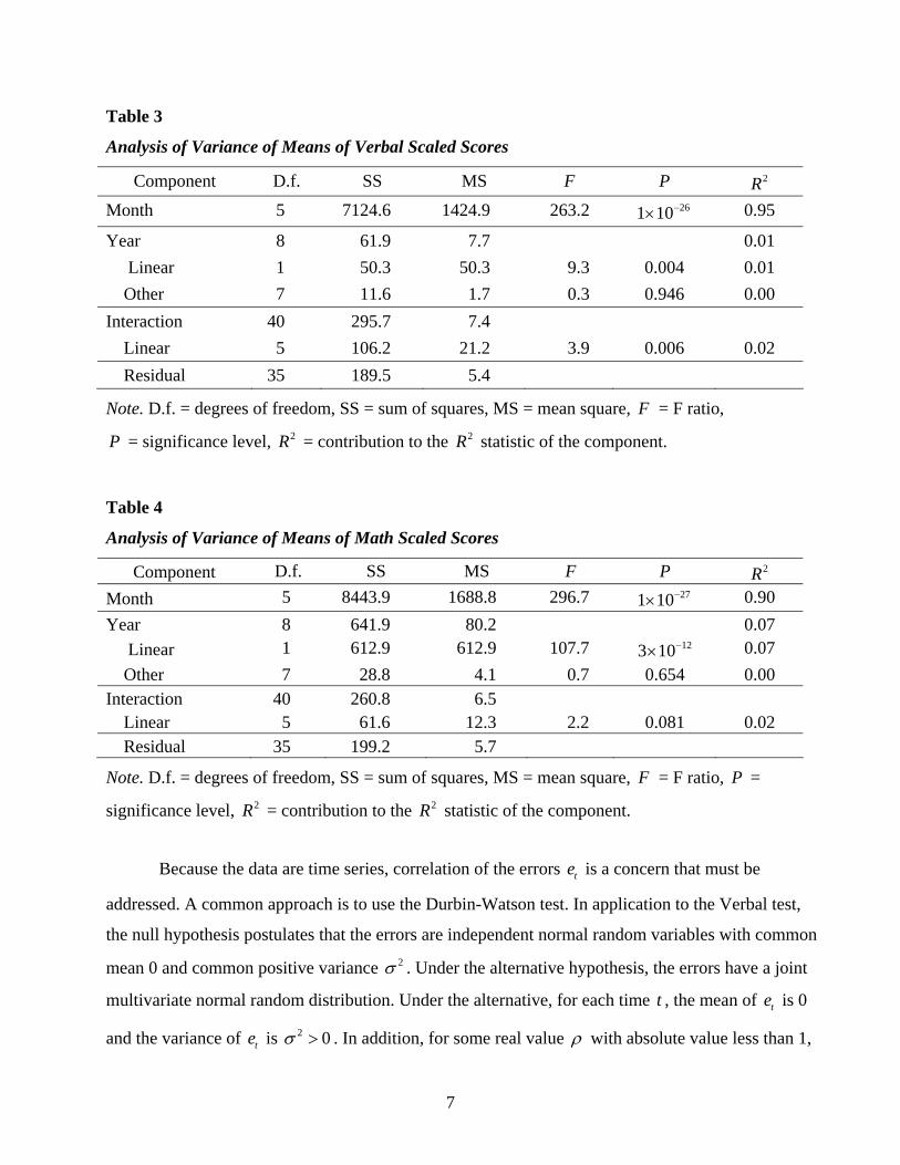
3.1 Analysis of Means of Scale Scores

For both the Verbal and Math means of scaled scores, the principal source of variability

is the month of administration. Some variability can also be ascribed to the year of

administration. Tables 1 and 2 provide summary statistics by month and by year, respectively.

Tables 3 and 4 provide an analysis of variance for Verbal and Math means to clarify the impact

of the different sources of variability present in the data. In the analysis of variance, effects for

year are decomposed into linear effects and nonlinear effects, while the two-factor interaction of

month and year is decomposed into month-by-linear-year and residual components. The linear

effects of year are used to study general trends. The month-by-linear-year component is

employed to assess trends specific to particular months of administration. The residual

component of the interaction is assumed to be a random error term. For example, the analysis of

variance for Verbal uses the model

( ) ( ) ( )( ) ( ) .t m t y t m t tV y t y t eμ α β γ δ= + + + + + (1)

To provide identifiable parameters, it is assumed that

4 4 661 4 4 1

0.i i j j ij j ijα γ γ δ= =− =− =

= = = =∑ ∑ ∑ ∑ (2)

As is customary in analysis of variance, the errors te are assumed to be independent and to have

mean 0 and common variance 2σ . The ( )m tα term corresponds to a month effect. The year effect

is ( )( ) .y ty tβ γ+ The interaction ( ) ( )m t y tδ is assumed to be linear in the year code ( )y t .

The tables show that month of administration is by far the most important source of

variation in means of scaled scores. The contrast between October and December is especially

striking. Some variation that is related to year of administration can be observed. This variation

involves an overall trend toward increasing scores, but this effect is small. For Verbal, 0.4 is the

least-squares estimate of the linear increase per yearβ of mean scaled score. The corresponding

figure for Math is 1.3, a larger but still small value. These small average increases vary

appreciably for different months. For Verbal, they range from 1.0 in March/April to –0.4 in May.

For Math, average increases per year range from 1.7 for December to 0.7 in November. In all,

the model used in the analysis of variance accounts for 97.5% of the variability in the Verbal

means and 97.9% of the variability in the Math means. Verbal and Math fluctuations are highly

6

correlated. The sample correlation for the pairs ( , )t tV M , 1 54,t≤ ≤ is 0.959. This correlation

reflects a very strong sample correlation of 0.993 in the monthly means and a strong sample

correlation of 0.871 in the yearly means. The sample correlation of the residual components for

Verbal and Math is only 0.372.

Table 1

Summary Statistics of Means of Scaled Scores by Month of Administration

Verbal Math Month Mean SD Mean SD

March/April 514.3 3.5 522.6 5.0 May 512.8 2.2 522.8 2.9 June 503.9 2.3 511.1 4.5 October 518.3 3.4 528.6 4.7 November 496.8 6.6 501.8 2.2 December 485.0 4.2 493.5 5.7 Total 505.2 11.9 513.4 13.3

Table 2

Summary Statistics of Means of Scaled Scores by Year of Administration

Verbal Math Year Mean SD Mean SD

1995 503.9 12.7 507.3 13.9 1996 504.3 11.3 510.1 13.1 1997 504.4 13.8 512.1 14.5 1998 505.0 12.2 510.8 12.0 1999 504.5 12.1 513.4 13.8 2000 505.8 14.8 514.6 16.3 2001 505.2 12.5 516.1 15.1 2002 506.1 11.6 517.0 13.9 2003 507.5 14.0 518.8 12.0 Total 505.2 11.9 513.4 13.3

7

Table 3

Analysis of Variance of Means of Verbal Scaled Scores

Component D.f. SS MS F P 2R Month 5 7124.6 1424.9 263.2 261 10−× 0.95

Year 8 61.9 7.7 0.01 Linear 1 50.3 50.3 9.3 0.004 0.01 Other 7 11.6 1.7 0.3 0.946 0.00 Interaction 40 295.7 7.4 Linear 5 106.2 21.2 3.9 0.006 0.02 Residual 35 189.5 5.4

Note. D.f. = degrees of freedom, SS = sum of squares, MS = mean square, F = F ratio,

P = significance level, 2R = contribution to the 2R statistic of the component.

Table 4

Analysis of Variance of Means of Math Scaled Scores

Component D.f. SS MS F P 2R Month 5 8443.9 1688.8 296.7 271 10−× 0.90 Year 8 641.9 80.2 0.07 Linear 1 612.9 612.9 107.7 123 10−× 0.07 Other 7 28.8 4.1 0.7 0.654 0.00 Interaction 40 260.8 6.5 Linear 5 61.6 12.3 2.2 0.081 0.02 Residual 35 199.2 5.7

Note. D.f. = degrees of freedom, SS = sum of squares, MS = mean square, F = F ratio, P =

significance level, 2R = contribution to the 2R statistic of the component.

Because the data are time series, correlation of the errors te is a concern that must be

addressed. A common approach is to use the Durbin-Watson test. In application to the Verbal test,

the null hypothesis postulates that the errors are independent normal random variables with common

mean 0 and common positive variance 2σ . Under the alternative hypothesis, the errors have a joint

multivariate normal random distribution. Under the alternative, for each time t , the mean of te is 0

and the variance of te is 2 0σ > . In addition, for some real value ρ with absolute value less than 1,

8

the correlation of te and t he + , 1 t t h T≤ < + ≤ , is hρ , so that the differences 1t te eρ −− are

independent random variables for 2 t T≤ ≤ , and ρ , the correlation of te and 1te + , is the serial

correlation of the residuals. All standard statistical software packages have provisions for

implementation of the Durbin-Watson test, although some variations exist concerning computations

of significance levels. In this report, results reported by SAS are employed. In the Math test, the

Durbin-Watson statistic has an approximate two-sided significance level of 0.14 and the estimated

serial correlation is 0.00. In the Verbal case, the corresponding significance level is 0.28 and the

estimated serial correlation is -0.32. It should be noted that considerable uncertainty concerning the

true serial correlation exists due to the small sample size of 54 and the 18 degrees of freedom, so that

inability to reject the null hypothesis does not imply that the serial correlation must be small. Actual

negative serial correlations would suggest a tendency for successive errors to change sign; however,

it should be emphasized that it is far from clear what the actual serial correlation is.

The basic results are clear. The primary variations in mean scaled scores involve month

of administration, but some quite modest yearly trends are present. Evidence exists for the

Verbal test of an interaction of yearly trends and month of administration. The evidence for the

Math test is weaker for the presence of this interaction. The estimated standard deviation of error

in the Verbal test is about 2.3. The corresponding standard deviation for the Math test is about

2.4. These standard deviations are quite small given that scales were set for the reference

population so that examinees for each test would have a standard deviation of 110.

3.2. Analysis of Raw-to-Scale Conversions

Raw-to-scale conversions for individual score have far less variability attributable to

month of administration or to yearly trend than is the case for mean scaled scores, although

conversions for a given raw score do not in all cases appear to be distributed as independent and

identically distributed normal random variables. Reduced variability of conversions is not

surprising for the SAT tests under study; new forms are constructed from items previously

pretested on large samples of examinees. In addition, established specifications are used for the

distribution of estimated item statistics, equating of test forms is based on large samples, and the

SAT has a carefully constructed braiding plan.

Tables 5, 6, 7, and 8 provide some basic summaries of results for scale scores at each raw

score point. In Tables 7 and 8, the same model as that presented in Section 3.1, which was used

9

with means of scaled scores, is applied to conversions. Raw scores are excluded for a few

extreme scores in which the conversions were not available for some administration.

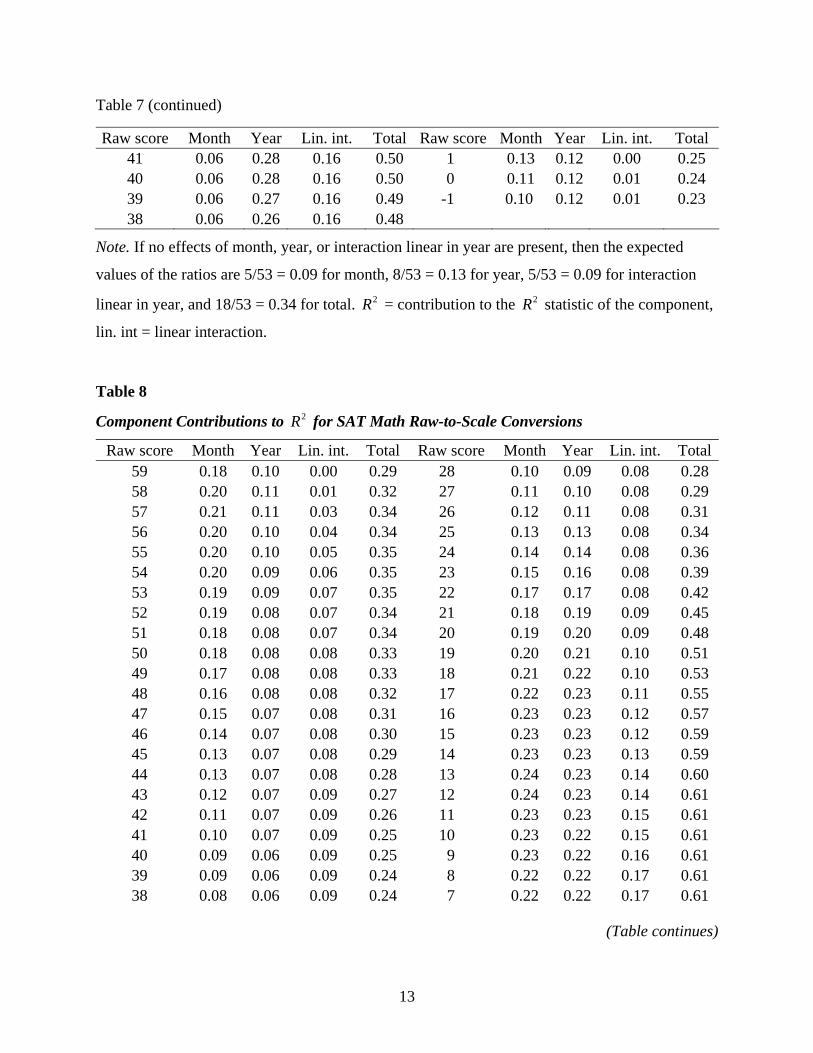
In examination of Tables 7 and 8, note that if no effects of month, year, or interaction linear

in year are present, then the expected values of the ratios are 5/53 = 0.09 for month, 8/53 = 0.13 for

year, 5/53 = 0.09 for interaction linear in year, and 18/53 = 0.34 for total. If conversions are

distributed as independent and identically distributed normal random variables, then standard

results from analysis of variance show that the probability is 0.05 that the model 2R exceeds 0.50.

Similarly, the probability is 0.05 that the 2R component for month or linear-year-by-month

interaction exceeds 0.20, and the probability is 0.05 that an 2R component for year exceeds 0.28.

Examined on an individual basis, numerous conversions for both Verbal and Math appear

incompatible with a trivial model. Precise evaluation of the situation is complicated by issues of

multiple comparisons. The Math test has 62 raw scores under study, and the Verbal test has 81 raw

scores under study; three 2R components and one overall 2R statistic are considered for each of

these raw scores. In addition, for any two raw scores, the time series of raw-to-scale conversions

for the same test are highly correlated, especially for raw scores that are close to each other.

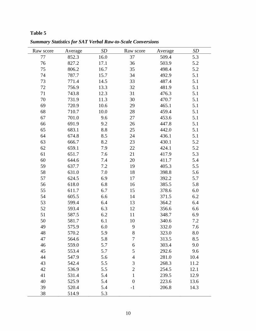
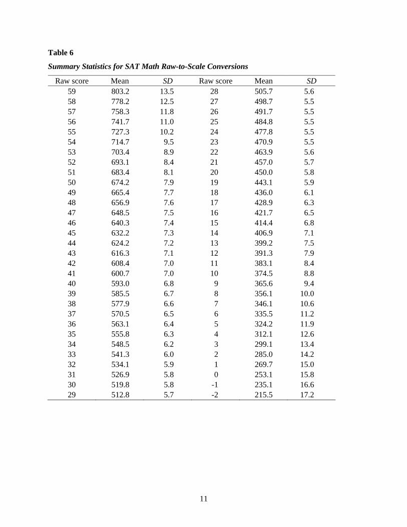
On the whole, Tables 5 to 8 provide a rather favorable picture in terms of test stability.

Except for very high or very low raw scores, raw-to-scale conversions exhibit quite limited

variability. The increased variability for very high or very low scores may result from nonlinearity

of scaling. For example, in the Verbal case, the average difference between the raw-to-scale

conversions for raw scores 76 and 75 is 21.1, whereas the average difference for raw scores 40 and

39 is 5.5. As noted earlier, the recentering of the SAT resulted in marked nonlinearity of the raw-

to-scale conversions in the tails of the raw score distributions for Verbal and Math.

As in the analysis of variance for mean scale scores, the issue of serial correlation arises. In

the case of raw-to-scale conversions, results are somewhat equivocal. No Durbin-Watson test for

a raw-to-scale conversion for Math is significant. For the Verbal test, the tests for raw scores

from 56 through 68 have two-sided significance levels less than 0.05, and the smallest observed

level is 0.016; the rest are greater than 0.05. Again, multiple comparisons is an issue. As already

noted, raw-to-scale conversions are quite highly correlated, especially in the case of conversions

for similar raw scores, and some 143 raw-to-scale conversions have been examined for the

Verbal and Math assessments. Thus it is not clear that serial correlation is actually an issue.

10

Table 5

Summary Statistics for SAT Verbal Raw-to-Scale Conversions

Raw score Average SD Raw score Average SD 77 852.3 16.0 37 509.4 5.3 76 827.2 17.1 36 503.9 5.2 75 806.2 16.7 35 498.4 5.2 74 787.7 15.7 34 492.9 5.1 73 771.4 14.5 33 487.4 5.1 72 756.9 13.3 32 481.9 5.1 71 743.8 12.3 31 476.3 5.1 70 731.9 11.3 30 470.7 5.1 69 720.9 10.6 29 465.1 5.1 68 710.7 10.0 28 459.4 5.1 67 701.0 9.6 27 453.6 5.1 66 691.9 9.2 26 447.8 5.1 65 683.1 8.8 25 442.0 5.1 64 674.8 8.5 24 436.1 5.1 63 666.7 8.2 23 430.1 5.2 62 659.1 7.9 22 424.1 5.2 61 651.7 7.6 21 417.9 5.3 60 644.6 7.4 20 411.7 5.4 59 637.7 7.2 19 405.3 5.5 58 631.0 7.0 18 398.8 5.6 57 624.5 6.9 17 392.2 5.7 56 618.0 6.8 16 385.5 5.8 55 611.7 6.7 15 378.6 6.0 54 605.5 6.6 14 371.5 6.2 53 599.4 6.4 13 364.2 6.4 52 593.4 6.3 12 356.6 6.6 51 587.5 6.2 11 348.7 6.9 50 581.7 6.1 10 340.6 7.2 49 575.9 6.0 9 332.0 7.6 48 570.2 5.9 8 323.0 8.0 47 564.6 5.8 7 313.5 8.5 46 559.0 5.7 6 303.4 9.0 45 553.4 5.7 5 292.6 9.6 44 547.9 5.6 4 281.0 10.4 43 542.4 5.5 3 268.3 11.2 42 536.9 5.5 2 254.5 12.1 41 531.4 5.4 1 239.5 12.9 40 525.9 5.4 0 223.6 13.6 39 520.4 5.4 -1 206.8 14.3 38 514.9 5.3

11

Table 6

Summary Statistics for SAT Math Raw-to-Scale Conversions

Raw score Mean SD Raw score Mean SD 59 803.2 13.5 28 505.7 5.6 58 778.2 12.5 27 498.7 5.5 57 758.3 11.8 26 491.7 5.5 56 741.7 11.0 25 484.8 5.5 55 727.3 10.2 24 477.8 5.5 54 714.7 9.5 23 470.9 5.5 53 703.4 8.9 22 463.9 5.6 52 693.1 8.4 21 457.0 5.7 51 683.4 8.1 20 450.0 5.8 50 674.2 7.9 19 443.1 5.9 49 665.4 7.7 18 436.0 6.1 48 656.9 7.6 17 428.9 6.3 47 648.5 7.5 16 421.7 6.5 46 640.3 7.4 15 414.4 6.8 45 632.2 7.3 14 406.9 7.1 44 624.2 7.2 13 399.2 7.5 43 616.3 7.1 12 391.3 7.9 42 608.4 7.0 11 383.1 8.4 41 600.7 7.0 10 374.5 8.8 40 593.0 6.8 9 365.6 9.4 39 585.5 6.7 8 356.1 10.0 38 577.9 6.6 7 346.1 10.6 37 570.5 6.5 6 335.5 11.2 36 563.1 6.4 5 324.2 11.9 35 555.8 6.3 4 312.1 12.6 34 548.5 6.2 3 299.1 13.4 33 541.3 6.0 2 285.0 14.2 32 534.1 5.9 1 269.7 15.0 31 526.9 5.8 0 253.1 15.8 30 519.8 5.8 -1 235.1 16.6 29 512.8 5.7 -2 215.5 17.2

12

Table 7

Component Contributions to 2R for SAT Verbal Raw-to-Scale Conversions

Raw score Month Year Lin. int. Total Raw score Month Year Lin. int. Total 77 0.15 0.12 0.18 0.45 37 0.06 0.25 0.16 0.47 76 0.17 0.15 0.14 0.46 36 0.06 0.24 0.16 0.46 75 0.16 0.17 0.12 0.45 35 0.06 0.23 0.16 0.45 74 0.16 0.19 0.10 0.45 34 0.06 0.22 0.15 0.44 73 0.16 0.20 0.09 0.45 33 0.07 0.21 0.15 0.42 72 0.16 0.21 0.08 0.45 32 0.07 0.19 0.15 0.41 71 0.16 0.22 0.08 0.45 31 0.07 0.18 0.14 0.40 70 0.16 0.22 0.07 0.45 30 0.07 0.17 0.14 0.38 69 0.16 0.23 0.07 0.45 29 0.08 0.16 0.14 0.37 68 0.15 0.23 0.07 0.45 28 0.08 0.14 0.13 0.35 67 0.15 0.23 0.07 0.45 27 0.08 0.13 0.13 0.34 66 0.14 0.24 0.07 0.44 26 0.09 0.12 0.12 0.33 65 0.13 0.24 0.07 0.44 25 0.10 0.10 0.12 0.32 64 0.12 0.24 0.07 0.43 24 0.10 0.09 0.12 0.31 63 0.12 0.24 0.07 0.43 23 0.11 0.08 0.11 0.30 62 0.11 0.25 0.07 0.42 22 0.11 0.07 0.11 0.30 61 0.10 0.25 0.08 0.42 21 0.12 0.06 0.11 0.29 60 0.09 0.25 0.08 0.42 20 0.13 0.06 0.11 0.29 59 0.09 0.25 0.08 0.42 19 0.13 0.05 0.10 0.29 58 0.08 0.26 0.09 0.43 18 0.14 0.05 0.10 0.29 57 0.08 0.26 0.09 0.43 17 0.15 0.04 0.10 0.29 56 0.08 0.27 0.10 0.44 16 0.15 0.04 0.09 0.29 55 0.07 0.27 0.10 0.44 15 0.16 0.04 0.09 0.29 54 0.07 0.28 0.10 0.45 14 0.16 0.04 0.08 0.29 53 0.07 0.28 0.11 0.46 13 0.17 0.05 0.07 0.29 52 0.07 0.28 0.12 0.47 12 0.17 0.05 0.07 0.29 51 0.07 0.29 0.12 0.48 11 0.18 0.05 0.06 0.29 50 0.07 0.29 0.13 0.49 10 0.18 0.06 0.05 0.29 49 0.07 0.29 0.13 0.49 9 0.18 0.06 0.04 0.29 48 0.07 0.30 0.14 0.50 8 0.18 0.07 0.03 0.29 47 0.06 0.30 0.14 0.51 7 0.18 0.07 0.03 0.28 46 0.06 0.30 0.15 0.51 6 0.18 0.08 0.02 0.28 45 0.06 0.30 0.15 0.51 5 0.17 0.09 0.01 0.28 44 0.06 0.29 0.15 0.51 4 0.17 0.09 0.01 0.27 43 0.06 0.29 0.16 0.51 3 0.16 0.10 0.00 0.26 42 0.06 0.29 0.16 0.51 2 0.15 0.11 0.00 0.26

(Table continues)

13

Table 7 (continued)

Raw score Month Year Lin. int. Total Raw score Month Year Lin. int. Total 41 0.06 0.28 0.16 0.50 1 0.13 0.12 0.00 0.25 40 0.06 0.28 0.16 0.50 0 0.11 0.12 0.01 0.24 39 0.06 0.27 0.16 0.49 -1 0.10 0.12 0.01 0.23 38 0.06 0.26 0.16 0.48

Note. If no effects of month, year, or interaction linear in year are present, then the expected

values of the ratios are 5/53 = 0.09 for month, 8/53 = 0.13 for year, 5/53 = 0.09 for interaction

linear in year, and 18/53 = 0.34 for total. 2R = contribution to the 2R statistic of the component,

lin. int = linear interaction.

Table 8

Component Contributions to 2R for SAT Math Raw-to-Scale Conversions

Raw score Month Year Lin. int. Total Raw score Month Year Lin. int. Total59 0.18 0.10 0.00 0.29 28 0.10 0.09 0.08 0.28 58 0.20 0.11 0.01 0.32 27 0.11 0.10 0.08 0.29 57 0.21 0.11 0.03 0.34 26 0.12 0.11 0.08 0.31 56 0.20 0.10 0.04 0.34 25 0.13 0.13 0.08 0.34 55 0.20 0.10 0.05 0.35 24 0.14 0.14 0.08 0.36 54 0.20 0.09 0.06 0.35 23 0.15 0.16 0.08 0.39 53 0.19 0.09 0.07 0.35 22 0.17 0.17 0.08 0.42 52 0.19 0.08 0.07 0.34 21 0.18 0.19 0.09 0.45 51 0.18 0.08 0.07 0.34 20 0.19 0.20 0.09 0.48 50 0.18 0.08 0.08 0.33 19 0.20 0.21 0.10 0.51 49 0.17 0.08 0.08 0.33 18 0.21 0.22 0.10 0.53 48 0.16 0.08 0.08 0.32 17 0.22 0.23 0.11 0.55 47 0.15 0.07 0.08 0.31 16 0.23 0.23 0.12 0.57 46 0.14 0.07 0.08 0.30 15 0.23 0.23 0.12 0.59 45 0.13 0.07 0.08 0.29 14 0.23 0.23 0.13 0.59 44 0.13 0.07 0.08 0.28 13 0.24 0.23 0.14 0.60 43 0.12 0.07 0.09 0.27 12 0.24 0.23 0.14 0.61 42 0.11 0.07 0.09 0.26 11 0.23 0.23 0.15 0.61 41 0.10 0.07 0.09 0.25 10 0.23 0.22 0.15 0.61 40 0.09 0.06 0.09 0.25 9 0.23 0.22 0.16 0.61 39 0.09 0.06 0.09 0.24 8 0.22 0.22 0.17 0.61 38 0.08 0.06 0.09 0.24 7 0.22 0.22 0.17 0.61

(Table continues)

14

Table 8 (continued)

Raw score Month Year Lin. int. Total Raw score Month Year Lin. int. Total37 0.08 0.06 0.09 0.23 6 0.21 0.22 0.18 0.61 36 0.08 0.06 0.10 0.23 5 0.20 0.22 0.18 0.61 35 0.08 0.06 0.10 0.23 4 0.20 0.23 0.18 0.60 34 0.08 0.06 0.10 0.23 3 0.19 0.23 0.18 0.60 33 0.08 0.06 0.09 0.24 2 0.19 0.23 0.17 0.59 32 0.08 0.06 0.09 0.24 1 0.19 0.23 0.16 0.58 31 0.09 0.07 0.09 0.25 0 0.19 0.23 0.14 0.57 30 0.09 0.07 0.09 0.25 -1 0.20 0.23 0.12 0.55 29 0.10 0.08 0.08 0.26 -2 0.20 0.21 0.10 0.51

Note. If no effects of month, year, or interaction linear in year are present, then the expected

values of the ratios are 5/53 = 0.09 for month, 8/53 = 0.13 for year, 5/53 = 0.09 for interaction

linear in year, and 18/53 = 0.34 for total. 2R = contribution to the 2R statistic of the component,

lin. int = linear interaction.

for similar raw scores, and some 143 raw-to-scale conversions have been examined for the Verbal

and Math assessments. Thus it is not clear that serial correlation is actually an issue.

The small variability in raw-to-scale conversions and the small residual variance in mean

scaled scores together suggest that test construction and equating are quite effective for the time

period under study. Recall that raw-to-scale conversions include random components reflecting

actual form difficulty, sampling errors in equating, and model errors in equating. Presumably each

component must be less variable than the observed conversion. Similarly, the residual variability

of the mean scaled score reflects sampling errors in equating, sampling errors in computation of

means, model errors in equating, and deviations from the model used in the analysis of variance.

Once again, the components should be less variable than the observed residual.

4. Analysis of Lagged Mean Squared Error

An additional summary of the raw-to-scale conversions can be employed to indicate the

extent to which raw-to-scale conversions that are less separated by time tend to be more similar than

are corresponding raw-to-scale conversions that are more separated by time. For this purpose, some

measures based on mean squared error are introduced. Consider the raw-to-scale conversion jtC for

raw score j for administration t of the SAT Verbal. Let h be a positive integer less than the

15

number 54T = of administrations under study. Then the average squared difference 2( )( )j t h jtC C+ −

between the raw-to-scale conversions at administrations t and t h+ for 1 t T h≤ ≤ − is

1 2( )

1( ) ( ) .

T h

jh j t h jtt

S T h C C−

−+

=

= − −∑ (3)

Thus jhS may be termed the mean square difference for lag .h A weighted average of the mean

squared differences jhS is twice the sample variance 2js of the raw-to-scale conversions jtC for

raw score j . To verify this claim, observe that summation of ( ) jhT h S− for 1 1h T≤ ≤ − yields

the sum of all differences 2( )jt juC C− for 1 .t u T≤ < ≤ Because the variance of the difference of

two independent and identically distributed random variables is twice the variance of each of the

individual variables, it follows that

1-1 2

1[T(T-1)/2] ( ) 2

T

jh jh

T h S s−

=

− =∑ (4)

(Hoeffding, 1948). If, for some raw score j , the raw-to-scale conversions jtC are independent and

identically distributed random variables with common variance 2jσ , then each jhS has expected

value 22 .jσ In this case, raw-to-scale conversions do not depend on time or time lags. Several

simple cases arise in which the expected value of the mean square difference jhS increases as the

lag h increases. One simple case involves a linear drift. If the raw-to-scale conversions jtC are

independent, have common variance 2 ,jσ and have respective means ,j ja tβ+ then the expected

value of jhS is 2 2 22 .j hσ β+ A cumulative component provides a second example. If the raw-to-

scale conversions jtC equal ,jt jtA B+ where the jtA have common mean jμ and common

variance jτ , 1jB is 0, the differences ( 1)j t jtB B+ − have common mean 0, common variance jυ , and

are uncorrelated, and the jtA and juB are uncorrelated for any times t and u , then the expected

value of jhS is a linear function 2 22 j jhτ υ+ of the lag h . One simple analysis of the mean square

differences considers a linear prediction of 2( )( )j t h jtC C+ − by the lag h . Use of standard formulas

for sums of powers of integers (Courant, 1937, pp. 27–28) shows that

16

1 2 21( )( / 2) ( 1)( 2) / 24,T

hT h h T T T T−

=− − = − −∑ (5)

so that the slope is estimated by least squares to be

12 1

124[ ( 1)( 2)] ( / 2)( ) .

T

j jhh

U T T T h T T h S−

−

=

= − − − −∑ (6)

Examination of the jU can help indicate whether mean squared differences tend to increase with

increasing lags. For lag h , the fitted mean squared difference is 22 ( / 2)j js U h T+ − . Thus 22 js is

the average fitted mean squared difference over lags h from 1 to 1T − . Tables 9 and 10

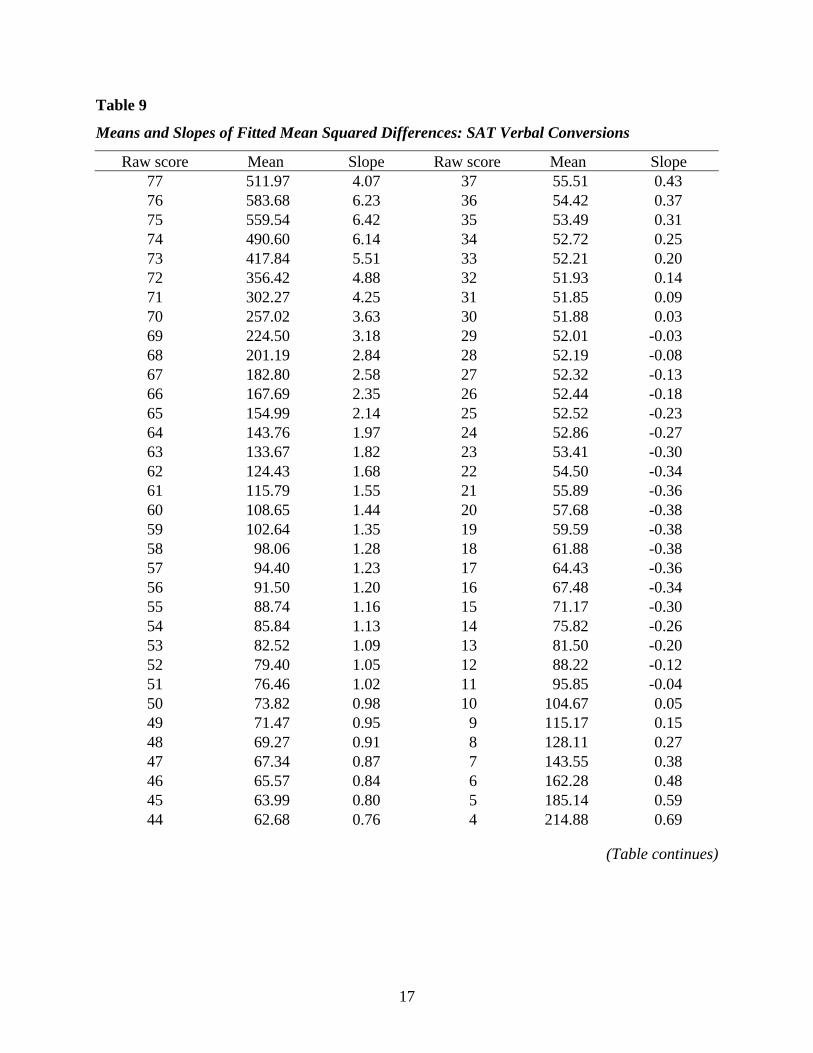
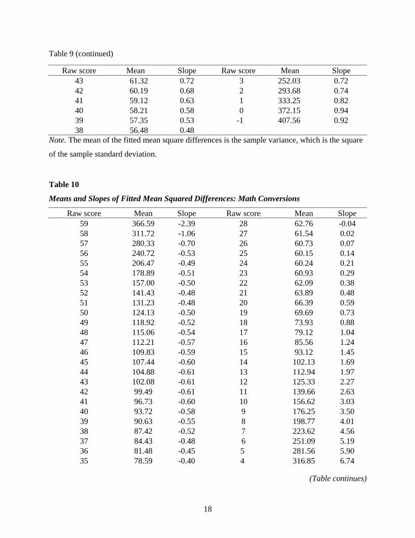
summarize results for SAT Verbal and SAT Math conversions.

As indicated earlier, the variations in means of fitted mean squared differences (sample

variances) appear to reflect the results of SAT recentering. Although it is reasonable to expect

positive slopes, it is noteworthy that many observed slopes are negative, especially for the Math

test. Nevertheless, the negative slopes are relatively small in magnitude, especially when

compared to means. In the case of SAT Verbal, positive slopes can be as large as 1.5% of the

means. For example, consider the case of raw score 67 (see Table 9). In this case, the ratio of

slope to mean is 1.4%. The fitted mean square differences range from 115.83 for a lag of 1 to

249.78 for a lag of 53. This result is compatible with a substantial increase in mean square

difference for higher lags, although this increase is somewhat less impressive in terms of the root

mean square differences obtained by taking square roots of mean squared differences. In this

case, root mean square differences range from 10.8 for a lag of 1 to 15.8 for a lag of 53. In the

case of SAT Math, positive slopes can be as high as 2.1% of the means. The most notable

positive slopes are encountered for very low scores. For example, for a raw score of 2, the ratio

of slope to mean is 2.1%, the fitted mean square differences range from 178.69 for a lag of 1 to

627.35 for a lag of 53. The corresponding range for root mean square differences is from 13.37

for a lag of 1 to 25.05 for a lag of 53. This level of variability is relatively large, although it

corresponds to an average scale score of 284.97 that is far below scores likely to be regarded as

even marginally acceptable by academic institutions. In the analysis of extreme cases, selection

bias must be considered. Thus the analysis of mean square differences does not indicate any

major difficulties with stability of raw-to-scale conversions within the period under study.

17

Table 9

Means and Slopes of Fitted Mean Squared Differences: SAT Verbal Conversions

Raw score Mean Slope Raw score Mean Slope 77 511.97 4.07 37 55.51 0.43 76 583.68 6.23 36 54.42 0.37 75 559.54 6.42 35 53.49 0.31 74 490.60 6.14 34 52.72 0.25 73 417.84 5.51 33 52.21 0.20 72 356.42 4.88 32 51.93 0.14 71 302.27 4.25 31 51.85 0.09 70 257.02 3.63 30 51.88 0.03 69 224.50 3.18 29 52.01 -0.03 68 201.19 2.84 28 52.19 -0.08 67 182.80 2.58 27 52.32 -0.13 66 167.69 2.35 26 52.44 -0.18 65 154.99 2.14 25 52.52 -0.23 64 143.76 1.97 24 52.86 -0.27 63 133.67 1.82 23 53.41 -0.30 62 124.43 1.68 22 54.50 -0.34 61 115.79 1.55 21 55.89 -0.36 60 108.65 1.44 20 57.68 -0.38 59 102.64 1.35 19 59.59 -0.38 58 98.06 1.28 18 61.88 -0.38 57 94.40 1.23 17 64.43 -0.36 56 91.50 1.20 16 67.48 -0.34 55 88.74 1.16 15 71.17 -0.30 54 85.84 1.13 14 75.82 -0.26 53 82.52 1.09 13 81.50 -0.20 52 79.40 1.05 12 88.22 -0.12 51 76.46 1.02 11 95.85 -0.04 50 73.82 0.98 10 104.67 0.05 49 71.47 0.95 9 115.17 0.15 48 69.27 0.91 8 128.11 0.27 47 67.34 0.87 7 143.55 0.38 46 65.57 0.84 6 162.28 0.48 45 63.99 0.80 5 185.14 0.59 44 62.68 0.76 4 214.88 0.69

(Table continues)

18

Table 9 (continued)

Raw score Mean Slope Raw score Mean Slope 43 61.32 0.72 3 252.03 0.72 42 60.19 0.68 2 293.68 0.74 41 59.12 0.63 1 333.25 0.82 40 58.21 0.58 0 372.15 0.94 39 57.35 0.53 -1 407.56 0.92 38 56.48 0.48

Note. The mean of the fitted mean square differences is the sample variance, which is the square

of the sample standard deviation.

Table 10

Means and Slopes of Fitted Mean Squared Differences: Math Conversions

Raw score Mean Slope Raw score Mean Slope 59 366.59 -2.39 28 62.76 -0.04 58 311.72 -1.06 27 61.54 0.02 57 280.33 -0.70 26 60.73 0.07 56 240.72 -0.53 25 60.15 0.14 55 206.47 -0.49 24 60.24 0.21 54 178.89 -0.51 23 60.93 0.29 53 157.00 -0.50 22 62.09 0.38 52 141.43 -0.48 21 63.89 0.48 51 131.23 -0.48 20 66.39 0.59 50 124.13 -0.50 19 69.69 0.73 49 118.92 -0.52 18 73.93 0.88 48 115.06 -0.54 17 79.12 1.04 47 112.21 -0.57 16 85.56 1.24 46 109.83 -0.59 15 93.12 1.45 45 107.44 -0.60 14 102.13 1.69 44 104.88 -0.61 13 112.94 1.97 43 102.08 -0.61 12 125.33 2.27 42 99.49 -0.61 11 139.66 2.63 41 96.73 -0.60 10 156.62 3.03 40 93.72 -0.58 9 176.25 3.50 39 90.63 -0.55 8 198.77 4.01 38 87.42 -0.52 7 223.62 4.56 37 84.43 -0.48 6 251.09 5.19 36 81.48 -0.45 5 281.56 5.90 35 78.59 -0.40 4 316.85 6.74

(Table continues)

19

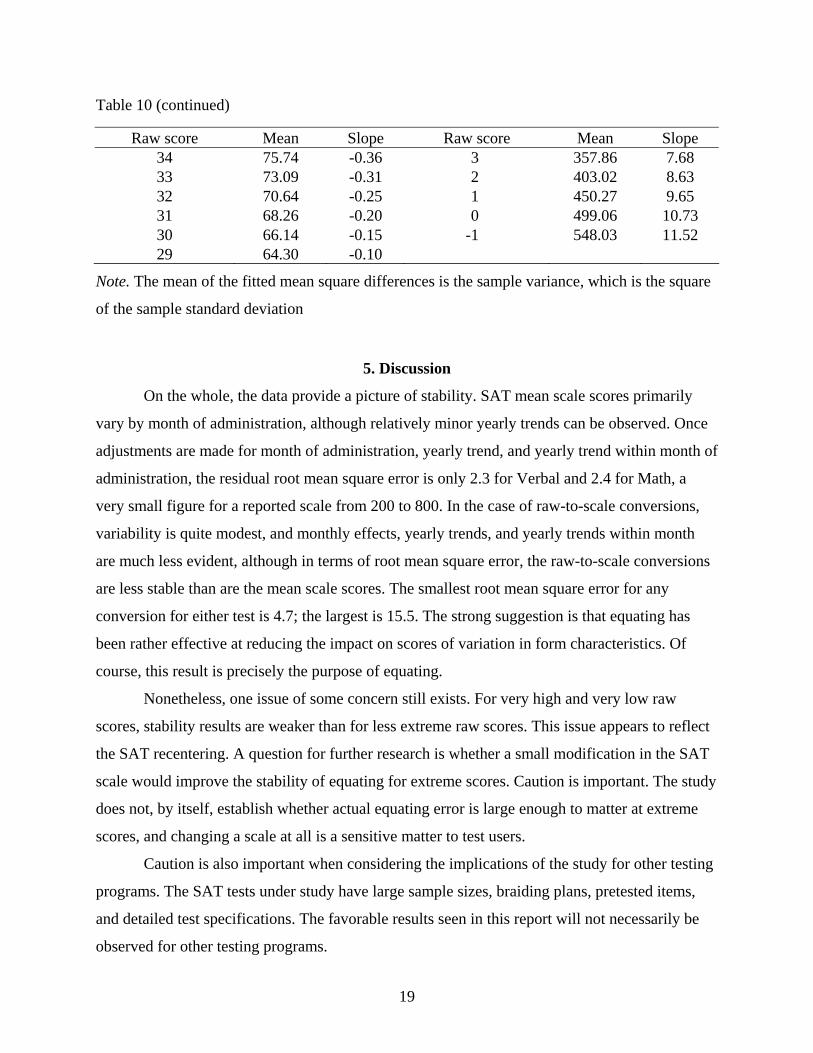
Table 10 (continued)

Raw score Mean Slope Raw score Mean Slope 34 75.74 -0.36 3 357.86 7.68 33 73.09 -0.31 2 403.02 8.63 32 70.64 -0.25 1 450.27 9.65 31 68.26 -0.20 0 499.06 10.73 30 66.14 -0.15 -1 548.03 11.52 29 64.30 -0.10

Note. The mean of the fitted mean square differences is the sample variance, which is the square

of the sample standard deviation

5. Discussion

On the whole, the data provide a picture of stability. SAT mean scale scores primarily

vary by month of administration, although relatively minor yearly trends can be observed. Once

adjustments are made for month of administration, yearly trend, and yearly trend within month of

administration, the residual root mean square error is only 2.3 for Verbal and 2.4 for Math, a

very small figure for a reported scale from 200 to 800. In the case of raw-to-scale conversions,

variability is quite modest, and monthly effects, yearly trends, and yearly trends within month

are much less evident, although in terms of root mean square error, the raw-to-scale conversions

are less stable than are the mean scale scores. The smallest root mean square error for any

conversion for either test is 4.7; the largest is 15.5. The strong suggestion is that equating has

been rather effective at reducing the impact on scores of variation in form characteristics. Of

course, this result is precisely the purpose of equating.

Nonetheless, one issue of some concern still exists. For very high and very low raw

scores, stability results are weaker than for less extreme raw scores. This issue appears to reflect

the SAT recentering. A question for further research is whether a small modification in the SAT

scale would improve the stability of equating for extreme scores. Caution is important. The study

does not, by itself, establish whether actual equating error is large enough to matter at extreme

scores, and changing a scale at all is a sensitive matter to test users.

Caution is also important when considering the implications of the study for other testing

programs. The SAT tests under study have large sample sizes, braiding plans, pretested items,

and detailed test specifications. The favorable results seen in this report will not necessarily be

observed for other testing programs.

20

References

Courant, R. (1937). Differential and integral calculus (2nd ed.). New York: Wiley Interscience.

Dorans, N. (2002a). Recentering and realigning the SAT score distributions: How and why?

Journal of Educational Measurement, 39, 59–84.

Dorans, N. (2002b). The recentering of SAT scales and its effects on score distributions and

score interpretations (College Board Research Rep. No. 2002-11). New York: The

College Board.

Draper, N. R., & Smith, H. (1998). Applied regression analysis (3rd ed.). New York: John

Wiley.

ETS. (2002). ETS standards for quality and fairness. Princeton, NJ: ETS.

Hoeffding, W. (1948). A class of statistics with asymptotically normal distributions. The Annals

of Mathematical Statistics, 19, 293–325.

Kolen, M. J. (2006). Scaling and norming. In R. L. Brennan (Ed.), Educational measurement

(4th ed., pp. 155–186). Westport, CT: Praeger.

Kolen, M. J., & Brennan, R. L. (2004). Test equating, scaling, and linking: Methods and

practices (2nd ed.). New York: Springer-Verlag.

Livingston, S. (2004). Equating test scores (without IRT). Princeton, NJ: ETS.

Liu, J., Curley, E., & Low, A. (2005). The study of SAT scale stability (ETS Statistical Rep. No.

SR-2005-72). Princeton, NJ: ETS.

McHale, F. J., & Ninneman, A. M. (1994). The stability of the score scale for the scholastic

aptitude test from 1973 to 1984 (ETS Statistical Rep. No. SR-94-27). Princeton, NJ: ETS.

Modu, C. C., & Stern, J. (1975). The stability of the SAT score scale (ETS Research Bulletin No.

RB-75-9). Princeton, NJ: ETS.

Petersen, N. S., Kolen, M. J., & Hoover, H. D. (1989). Scaling, norming, and equating. In R. L.

Linn (Ed.), Educational measurement (3rd ed., pp. 221–262). New York: Macmillan.

Stewart, E. E. (1966). The stability of the SAT-Verbal score scale (ETS Research Bulletin No.

RB-66-37). Princeton, NJ: ETS.