
Software Metric; defect removal efficiency, Cyclomate Complexity Defect Seeding Mutation Testing.
Title Slide
“Conservation of software defect and scale-free behaviourin software systems"
Les Hatton
CISM, Kingston [email protected]
Version 1.1: 26/Mar/2008
Kingston University CISM Faculty Research Seminar. . . . . . . . . . . . . . . . . . . . . . . . . . . . . . . . . . . . . . . . . . . . . . . . . . . . . . . . . . . . . . . . . . . . . . . . . . . . . . . . . . .
Overview
What is scale-free behaviour ?Examples from the real worldGeneral mathematical developmentApplication to software systemsWhere to go from here ?
What is scale-free behaviour ?
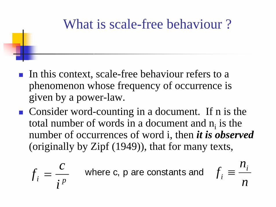
In this context, scale-free behaviour refers to a phenomenon whose frequency of occurrence is given by a power-law.Consider word-counting in a document. If n is the total number of words in a document and ni is the number of occurrences of word i, then it is observed(originally by Zipf (1949)), that for many texts,
pi icf = where c, p are constants and
nn
f ii ≡
What is scale-free behaviour ?
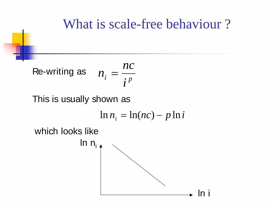
pi incn =Re-writing as
This is usually shown as
ipncni ln)ln(ln −=
which looks likeln ni
ln i
What is scale-free behaviour ?
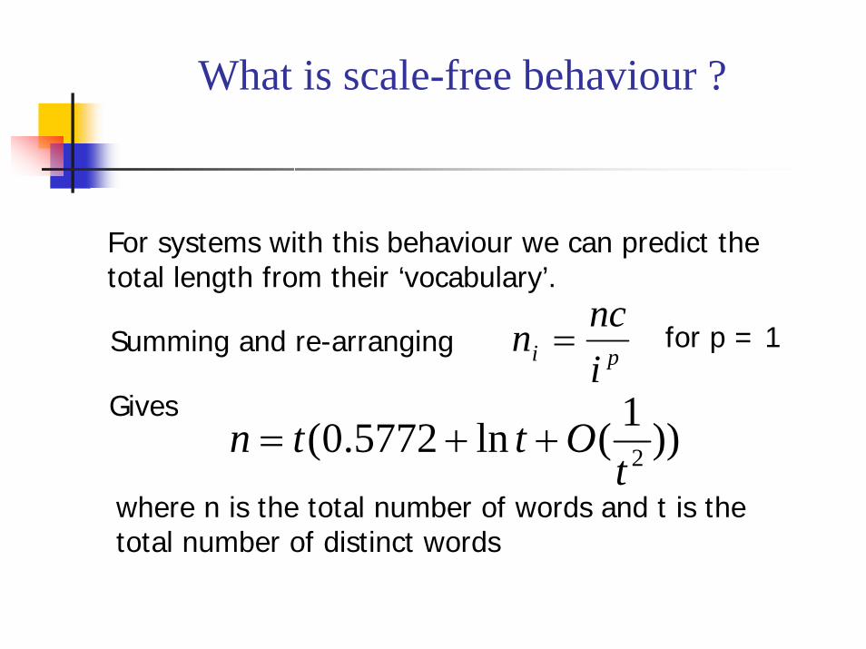
pi incn =
Gives
Summing and re-arranging
))1(ln5772.0( 2tOttn ++=
where n is the total number of words and t is thetotal number of distinct words
For systems with this behaviour we can predict the total length from their ‘vocabulary’.
for p = 1
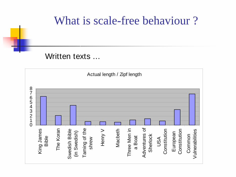
What is scale-free behaviour ?
Written texts …
Actual length / Zipf length
012345678
Kin
g Ja
mes
Bib
le
The
Kor
an
Sw
edis
h B
ible
(in S
wed
ish)
Tam
ing
of th
esh
rew
Hen
ry V
Mac
beth
Thre
e M
en in
a B
oat
Adv
entu
res
ofS
herlo
ck
US
AC
onst
itutio
n
Eur
opea
nC
onst
itutio
n
Com
mon
Vul
nera
bilit
ies
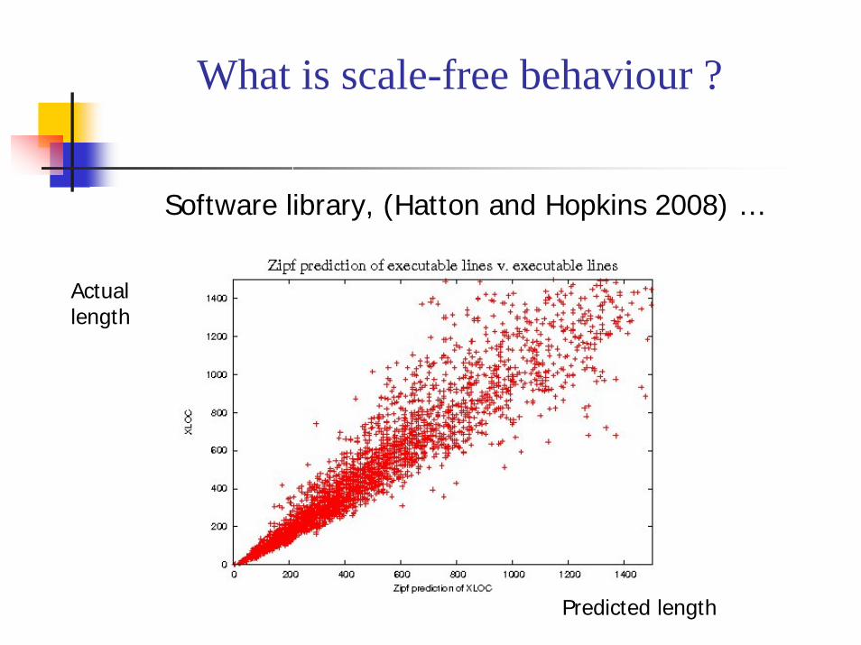
What is scale-free behaviour ?
Software library, (Hatton and Hopkins 2008) …
Actual length
Predicted length
Overview
What is scale-free behaviour ?Examples from the real worldGeneral mathematical developmentApplication to software systemsWhere to go from here ?
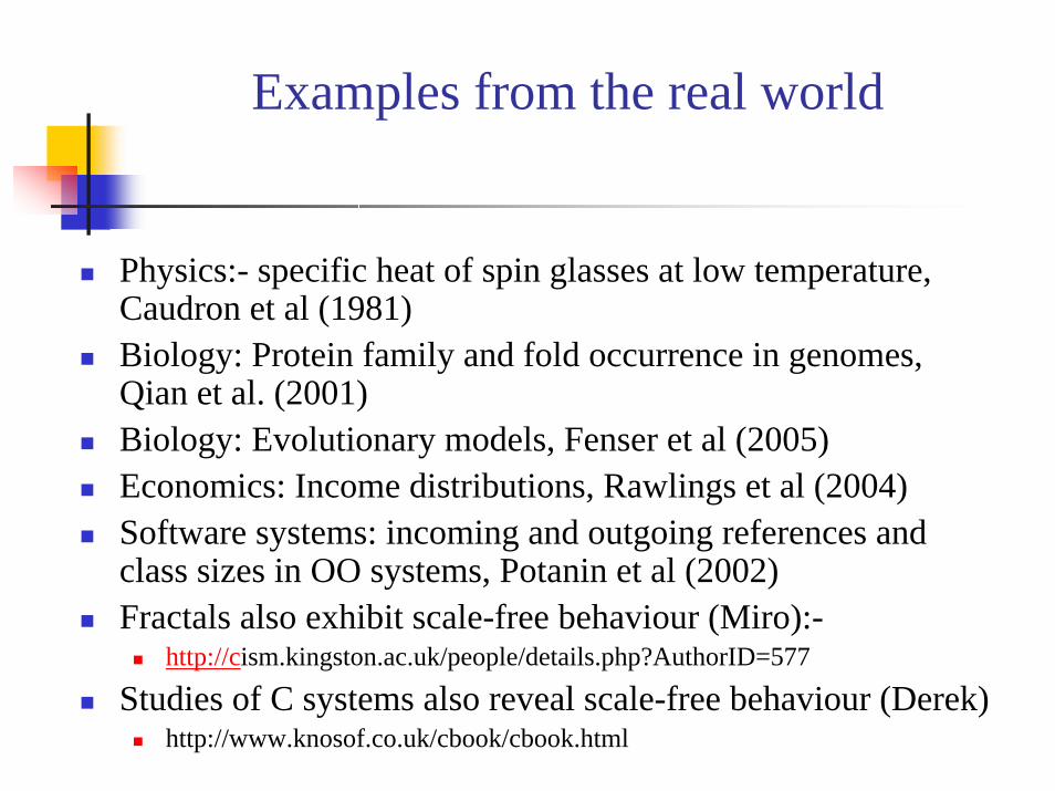
Examples from the real world
Physics:- specific heat of spin glasses at low temperature, Caudron et al (1981)Biology: Protein family and fold occurrence in genomes, Qian et al. (2001)Biology: Evolutionary models, Fenser et al (2005)Economics: Income distributions, Rawlings et al (2004)Software systems: incoming and outgoing references and class sizes in OO systems, Potanin et al (2002)Fractals also exhibit scale-free behaviour (Miro):-
http://cism.kingston.ac.uk/people/details.php?AuthorID=577
Studies of C systems also reveal scale-free behaviour (Derek)http://www.knosof.co.uk/cbook/cbook.html
Overview
What is scale-free behaviour ?Examples from the real worldGeneral mathematical developmentApplication to software systemsWhere to go from here ?
General mathematical treatment
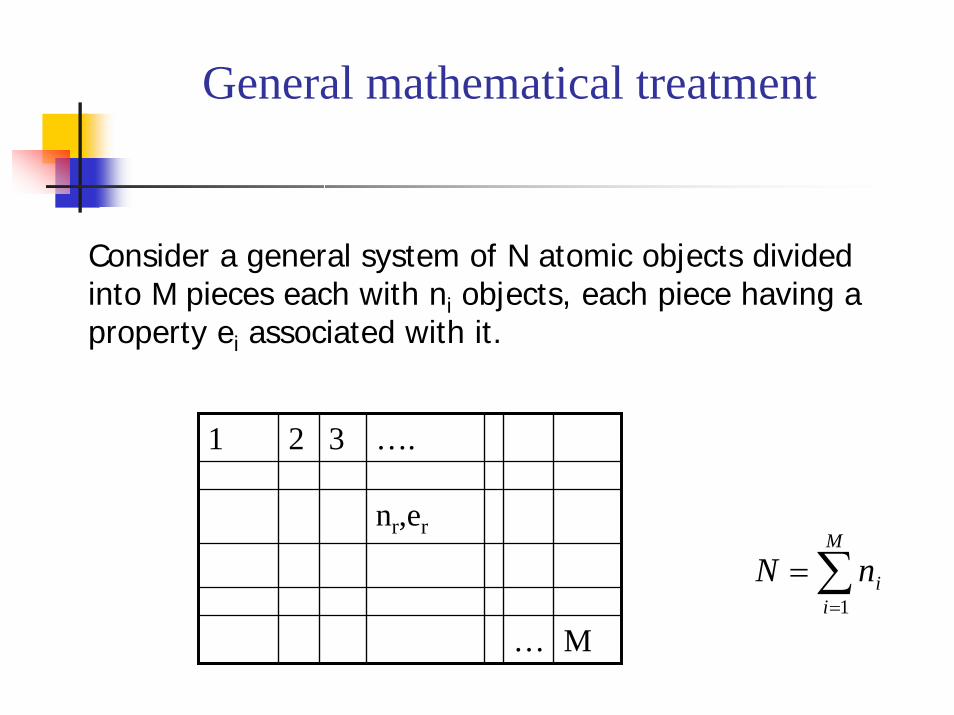
Consider a general system of N atomic objects dividedinto M pieces each with ni objects, each piece having aproperty ei associated with it.
1 2 3 ….
nr,er
… M
∑=
=M
iinN
1
General mathematical treatment
!!...!!
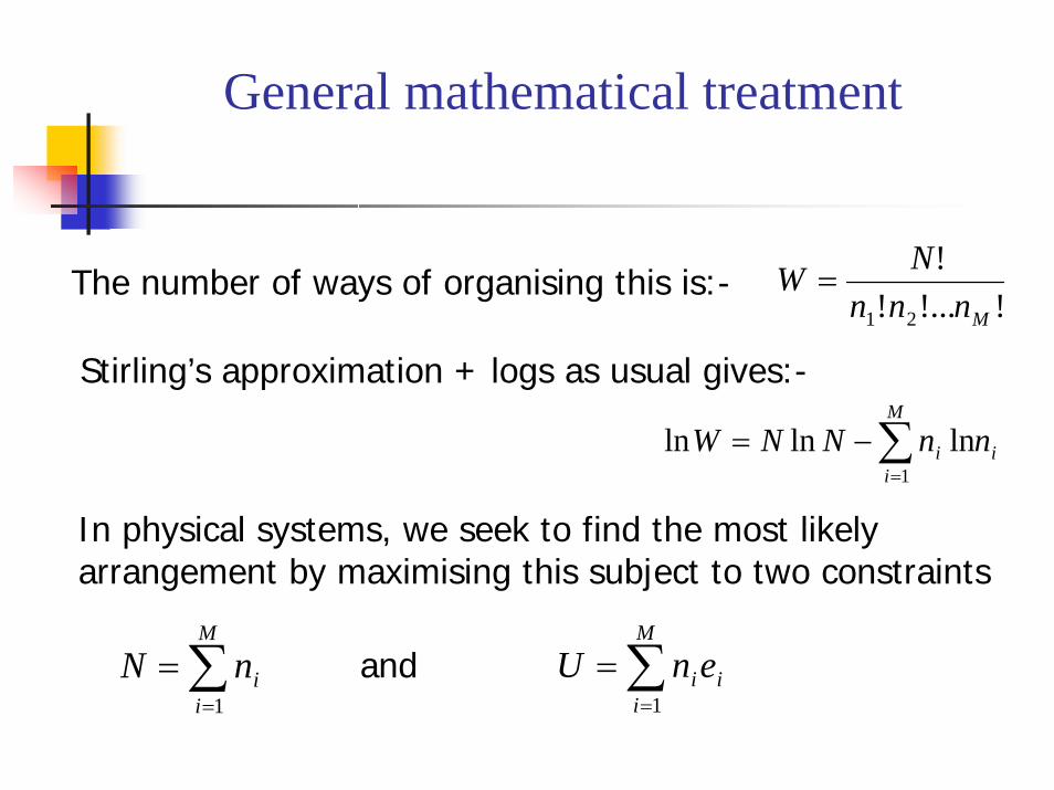
21 MnnnNW =The number of ways of organising this is:-
Stirling’s approximation + logs as usual gives:-
i
M
ii nnNNW ∑
=
−=1
lnlnln
In physical systems, we seek to find the most likelyarrangement by maximising this subject to two constraints
i
M
iienU ∑
=
=1
∑=
=M
iinN
1
and
General mathematical treatment
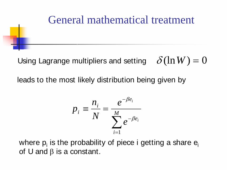
0)(ln =WδUsing Lagrange multipliers and setting
leads to the most likely distribution being given by
∑=
−
−
=≡ M
i
e
ei
ii
i
e
eNn
p
1
β
β
where pi is the probability of piece i getting a share eiof U and β is a constant.
General mathematical treatment
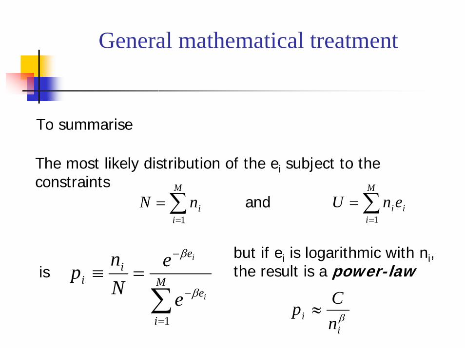
To summarise
The most likely distribution of the ei subject to theconstraints
i
M
iienU ∑
=
=1
∑=
=M
iinN
1and
but if ei is logarithmic with ni, the result is a power-law
∑=
−
−
=≡ M
i
e
ei
ii
i
e
eNn
p
1
β
β
is
βi
i nCp ≈
Overview
What is scale-free behaviour ?Examples from the real worldGeneral mathematical developmentApplication to software systemsWhere to go from here ?
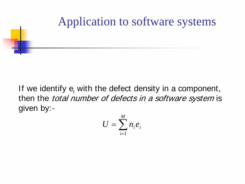
Application to software systems
If we identify ei with the defect density in a component,then the total number of defects in a software system isgiven by:-
i
M
iienU ∑
=
=1
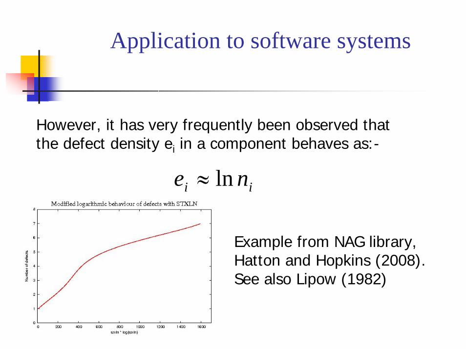
Application to software systems
However, it has very frequently been observed thatthe defect density ei in a component behaves as:-
ii ne ln≈
Example from NAG library, Hatton and Hopkins (2008). See also Lipow (1982)
Application to software systems
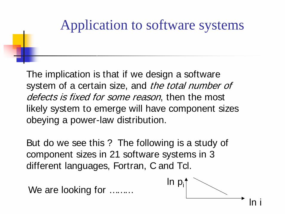
The implication is that if we design a software system of a certain size, and the total number of defects is fixed for some reason, then the most likely system to emerge will have component sizes obeying a power-law distribution.
But do we see this ? The following is a study of component sizes in 21 software systems in 3 different languages, Fortran, C and Tcl.
ln pi
ln iWe are looking for ………
Application to software systems
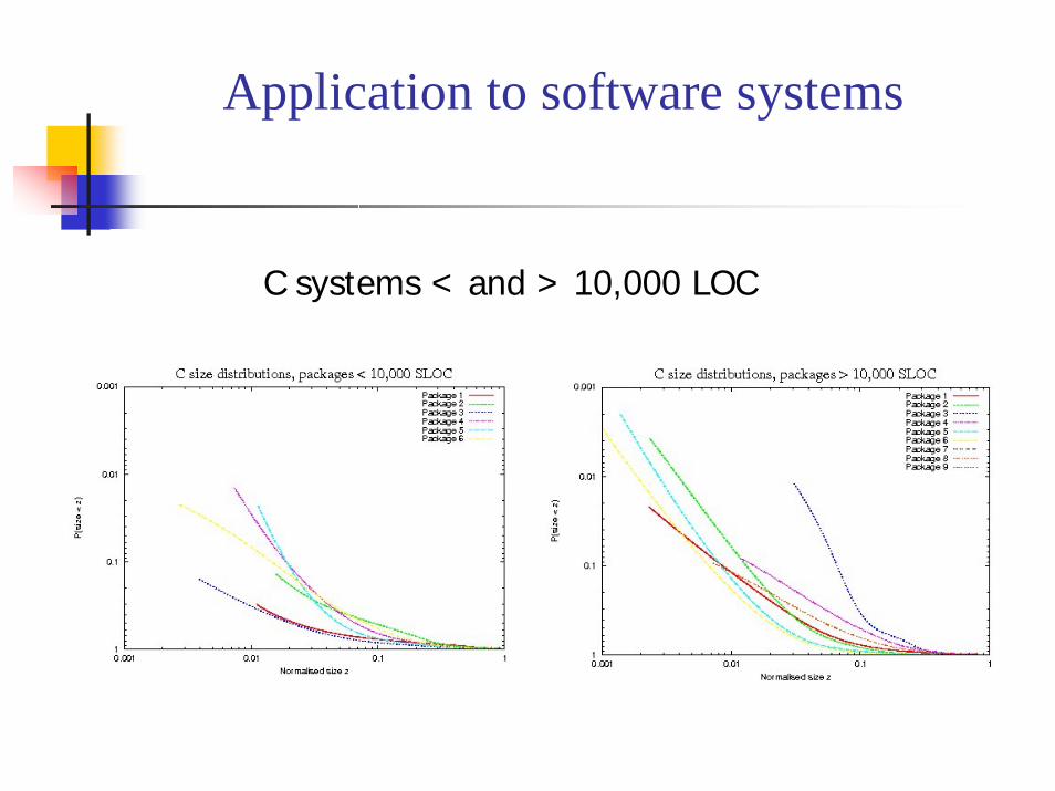
C systems < and > 10,000 LOC
Application to software systems
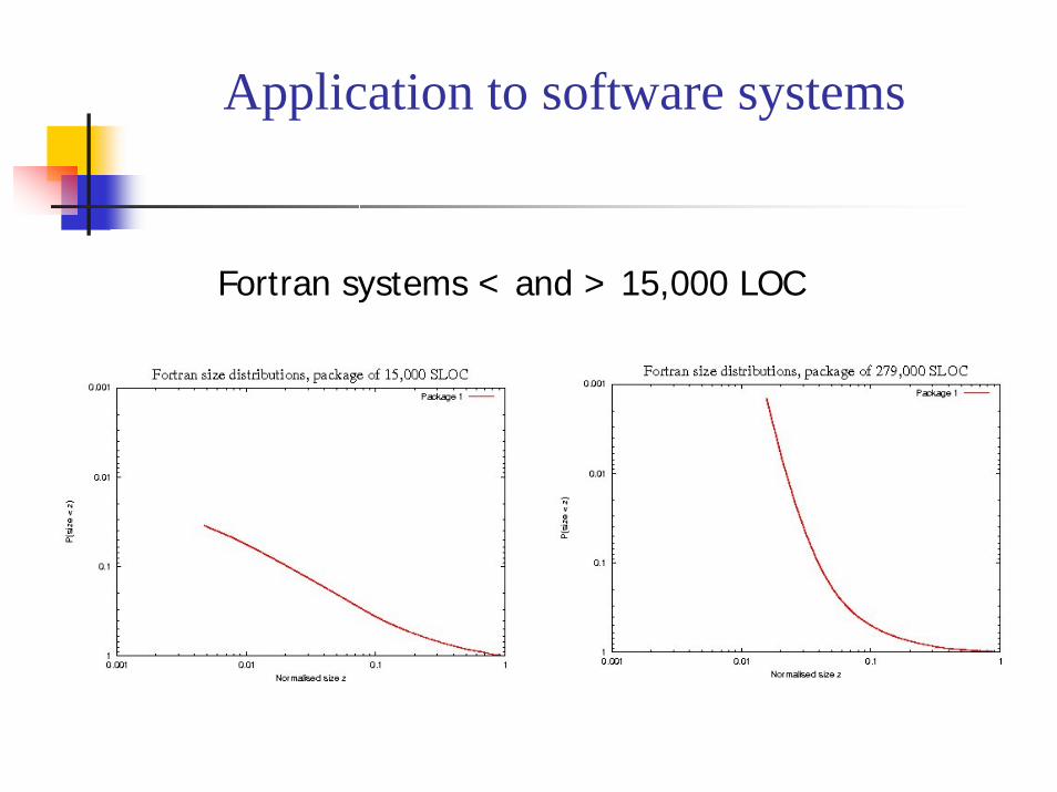
Fortran systems < and > 15,000 LOC
Application to software systems
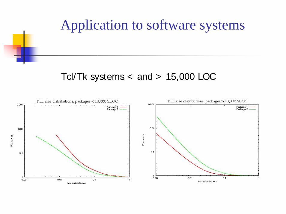
Tcl/Tk systems < and > 15,000 LOC
Overview
What is scale-free behaviour ?Examples from the real worldGeneral mathematical developmentApplication to software systemsWhere to go from here ?
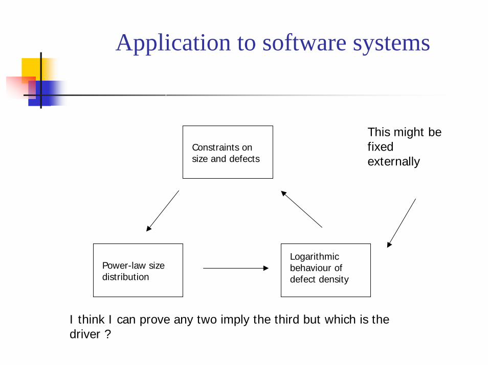
Application to software systems
This might be fixed externally
Constraints on size and defects
Power-law size distribution
Logarithmic behaviour of defect density
I think I can prove any two imply the third but which is the driver ?
Conclusions
Component sizes in software systems of very different size and language obey power-law distributionsStandard arguments from statistical mechanics show that this is inevitable if the total number of defects is approximately conserved.The analogy with statistical mechanics can be extended furtherMore experiments are necessary to determine the driver.