Conservation based uncertainty propagation in dynamic systems

UNLV Theses, Dissertations, Professional Papers, and Capstones

8-2010

Conservation based uncertainty propagation in dynamic systems Conservation based uncertainty propagation in dynamic systems

Lillian J. Ratliff University of Nevada, Las Vegas

Follow this and additional works at: https://digitalscholarship.unlv.edu/thesesdissertations

Part of the Controls and Control Theory Commons, Control Theory Commons, and the Dynamic

Systems Commons

Repository Citation Repository Citation Ratliff, Lillian J., "Conservation based uncertainty propagation in dynamic systems" (2010). UNLV Theses, Dissertations, Professional Papers, and Capstones. 867. http://dx.doi.org/10.34917/2213605

This Thesis is protected by copyright and/or related rights. It has been brought to you by Digital Scholarship@UNLV with permission from the rights-holder(s). You are free to use this Thesis in any way that is permitted by the copyright and related rights legislation that applies to your use. For other uses you need to obtain permission from the rights-holder(s) directly, unless additional rights are indicated by a Creative Commons license in the record and/or on the work itself. This Thesis has been accepted for inclusion in UNLV Theses, Dissertations, Professional Papers, and Capstones by an authorized administrator of Digital Scholarship@UNLV. For more information, please contact [email protected].

http://library.unlv.edu/

http://library.unlv.edu/

https://digitalscholarship.unlv.edu/thesesdissertations

https://digitalscholarship.unlv.edu/thesesdissertations?utm_source=digitalscholarship.unlv.edu%2Fthesesdissertations%2F867&utm_medium=PDF&utm_campaign=PDFCoverPages

http://network.bepress.com/hgg/discipline/269?utm_source=digitalscholarship.unlv.edu%2Fthesesdissertations%2F867&utm_medium=PDF&utm_campaign=PDFCoverPages




http://dx.doi.org/10.34917/2213605

mailto:[email protected]

CONSERVATION BASED UNCERTAINTY PROPAGATION IN DYNAMIC

SYSTEMS

by

Lillian J Ratliff

Bachelor of Science in Electrical EngineeringUniversity of Nevada, Las Vegas

2008

Bachelor of Science in MathematicsUniversity of Nevada, Las Vegas

2008

A thesis submitted in partial fulfillmentof the requirements for the

Masters of Science in Engineering

Department of Electrical and Computer Engineering

Howard R. Hughes College of Engineering

Graduate College

University of Nevada, Las Vegas

August 2010

Copyright by Lillian Ratliff 2010All Rights Reserved

ii

THE GRADUATE COLLEGE

We recommend the thesis prepared under our supervision by

Lillian J. Ratliff

entitled

Conservation Based Uncertainty Propagation in Dynamic Systems

be accepted in partial fulfillment of the requirements for the degree of

Master of Science in Engineering Electrical and Computer Engineering

Pushkin Kachroo, Committee Chair

Mehdi Ahmadian, Committee Member

Rama Venkat, Committee Member

Yahia Bagzouz, Committee Member

Mohammad Trabia, Graduate Faculty Representative

Ronald Smith, Ph. D., Vice President for Research and Graduate Studies

and Dean of the Graduate College

August 2010

ABSTRACT

Conservation Based Uncertainty Propagation in Dynamic Systems

by

Lillian J Ratliff

Dr. Pushkin Kachroo, Examination Committee ChairProfessor of Electrical and Computer Engineering

University of Nevada, Las Vegas

Uncertainty is present in our everyday decision making process as well as our

understanding of the structure of the universe. As a result an intense and mathemat-

ically rigorous study of how uncertainty propagates in the dynamic systems present

in our lives is warranted and arguably necessary. In this thesis we examine existing

methods for uncertainty propagation in dynamic systems and present the results of

a literature survey that justifies the development of a conservation based method of

uncertainty propagation. Conservation methods are physics based and physics drives

our understanding of the physical world. Thus, it makes perfect sense to formulate an

understanding of uncertainty propagation in terms of one of the fundamental concepts

in physics: conservation. We develop that theory for a small group of dynamic systems

which are fundamental. They include ordinary differential equations, finite difference

equations, differential inclusions and inequalities, stochastic differential equations,

and Markov chains. The study presented considers uncertainty propagation from the

initial condition where the initial condition is given as a prior distribution defined

within a probability structure. This probability structure is preserved in the sense

of measure. The results of this study are the first steps into a generalized theory for

uncertainty propagation using conservation laws. In addition, it is hoped that the

iii

results can be used in applications such as robust control design for everything from

transportation systems to financial markets.

iv

ACKNOWLEDGMENTS

I would like to thank the National Science Foundation (NSF) for providing the fund-

ing through the NSF graduate research fellowship program (grfp) for the research

presented in this thesis. I would also like to thank the Center for Vehicle Systems

and Safety at Virginia Tech, and NASA for providing funding prior to the NSF grfp.

I would like to thank my advisor, Dr. Pushkin Kachroo for the guidance he provided.

In addition, I would like to thank all my committee members for participating.

v

TABLE OF CONTENTS

ABSTRACT . . . . . . . . . . . . . . . . . . . . . . . . . . . . . . . . . . . . iii

ACKNOWLEDGMENTS . . . . . . . . . . . . . . . . . . . . . . . . . . . . . v

TABLE OF CONTENTS . . . . . . . . . . . . . . . . . . . . . . . . . . . . . vi

LIST OF FIGURES . . . . . . . . . . . . . . . . . . . . . . . . . . . . . . . . ix

CHAPTER 1 INTRODUCTION . . . . . . . . . . . . . . . . . . . . . . . . 1Definition of Uncertainty . . . . . . . . . . . . . . . . . . . . . . . . . . . . 2What is Uncertainty Propagation? . . . . . . . . . . . . . . . . . . . . . . 2

Conservation Based Uncertainty Propagation . . . . . . . . . . . . . 3Problem Statement . . . . . . . . . . . . . . . . . . . . . . . . . . . . . . . 4Outline of the Thesis . . . . . . . . . . . . . . . . . . . . . . . . . . . . . . 5Contributions . . . . . . . . . . . . . . . . . . . . . . . . . . . . . . . . . . 6

CHAPTER 2 BACKGROUND . . . . . . . . . . . . . . . . . . . . . . . . . 9Existing Methods . . . . . . . . . . . . . . . . . . . . . . . . . . . . . . . . 9

Monte Carlo Method . . . . . . . . . . . . . . . . . . . . . . . . . . . 9Polynomial Chaos . . . . . . . . . . . . . . . . . . . . . . . . . . . . . 12Bayesian Inference . . . . . . . . . . . . . . . . . . . . . . . . . . . . 16

Relevant Literature . . . . . . . . . . . . . . . . . . . . . . . . . . . . . . . 21Motivation and Research Goal . . . . . . . . . . . . . . . . . . . . . . . . . 23

CHAPTER 3 DYNAMIC SYSTEMS . . . . . . . . . . . . . . . . . . . . . 24Examples of Dynamic Systems . . . . . . . . . . . . . . . . . . . . . . . . . 24Ordinary Differential Equations . . . . . . . . . . . . . . . . . . . . . . . . 25

Pendulum . . . . . . . . . . . . . . . . . . . . . . . . . . . . . . . . . 26Van der Pol Oscillator . . . . . . . . . . . . . . . . . . . . . . . . . . 27ODE model of Traffic Flow . . . . . . . . . . . . . . . . . . . . . . . . 27

Finite Difference Equations . . . . . . . . . . . . . . . . . . . . . . . . . . 29FDEs Given by Affine Transformations . . . . . . . . . . . . . . . . . 29FDE Model of Traffic Flow . . . . . . . . . . . . . . . . . . . . . . . . 30

Differential Inequalities and Inclusions . . . . . . . . . . . . . . . . . . . . 31Examples of Differential Inclusions . . . . . . . . . . . . . . . . . . . 31Examples of Differential Inequalities . . . . . . . . . . . . . . . . . . . 32

Stochastic Differential Equations . . . . . . . . . . . . . . . . . . . . . . . 33Population Growth . . . . . . . . . . . . . . . . . . . . . . . . . . . . 34

Markov Chains . . . . . . . . . . . . . . . . . . . . . . . . . . . . . . . . . 35Two-State Markov Chain . . . . . . . . . . . . . . . . . . . . . . . . . 36

Summary . . . . . . . . . . . . . . . . . . . . . . . . . . . . . . . . . . . . 39

vi

CHAPTER 4 ORDINARY DIFFERENTIAL EQUATIONS . . . . . . . . . 40What are Ordinary Differential Equations? . . . . . . . . . . . . . . . . . . 40Propagation of Uncertainty in ODEs . . . . . . . . . . . . . . . . . . . . . 41Derivation of Liouville Equation . . . . . . . . . . . . . . . . . . . . . . . . 41Solution to the Liouville Equation . . . . . . . . . . . . . . . . . . . . . . . 46

Solution By Method of Characteristics . . . . . . . . . . . . . . . . . 47Verification of Solution . . . . . . . . . . . . . . . . . . . . . . . . . . 48

Summary . . . . . . . . . . . . . . . . . . . . . . . . . . . . . . . . . . . . 53

CHAPTER 5 FINITE DIFFERENCE EQUATIONS . . . . . . . . . . . . 54What are Finite Difference Equations? . . . . . . . . . . . . . . . . . . . . 54Uncertainty Propagation in Finite Difference Equations . . . . . . . . . . . 551-D Finite Difference Equation . . . . . . . . . . . . . . . . . . . . . . . . 56Higher Dimensional Finite Difference Equations . . . . . . . . . . . . . . . 58Systems of Finite Difference Equaitons . . . . . . . . . . . . . . . . . . . . 61Conservation Form . . . . . . . . . . . . . . . . . . . . . . . . . . . . . . . 64Summary . . . . . . . . . . . . . . . . . . . . . . . . . . . . . . . . . . . . 65

CHAPTER 6 DIFFERENTIAL INEQUALITIES AND INCLUSIONS . . . 66Set-Valued Maps . . . . . . . . . . . . . . . . . . . . . . . . . . . . . . . . 66What are Differential Inclusions? . . . . . . . . . . . . . . . . . . . . . . . 67

What are Differential Inequalities? . . . . . . . . . . . . . . . . . . . 68Uncertainty Propagation through differential inclusions . . . . . . . . . . . 68

Construction of Probability Space . . . . . . . . . . . . . . . . . . . . 72Conservation Form . . . . . . . . . . . . . . . . . . . . . . . . . . . . . . . 79Summary . . . . . . . . . . . . . . . . . . . . . . . . . . . . . . . . . . . . 80

CHAPTER 7 STOCHASTIC DIFFERENTIAL EQUATIONS . . . . . . . 81What are Stochastic Differential Equations? . . . . . . . . . . . . . . . . . 81Propagation of Uncertainty through SDEs . . . . . . . . . . . . . . . . . . 84Ito Calculus . . . . . . . . . . . . . . . . . . . . . . . . . . . . . . . . . . . 85

Ito’s Formula . . . . . . . . . . . . . . . . . . . . . . . . . . . . . . . 86Derivation of the Fokker-Planck Equation . . . . . . . . . . . . . . . . . . 88Conservation Form . . . . . . . . . . . . . . . . . . . . . . . . . . . . . . . 92Summary . . . . . . . . . . . . . . . . . . . . . . . . . . . . . . . . . . . . 93

CHAPTER 8 MARKOV CHAINS . . . . . . . . . . . . . . . . . . . . . . . 94What are Markov Chains? . . . . . . . . . . . . . . . . . . . . . . . . . . . 94Transition Probabilities . . . . . . . . . . . . . . . . . . . . . . . . . . . . 95Uncertainty Propagation in Markov Chains . . . . . . . . . . . . . . . . . . 96Conservation Form . . . . . . . . . . . . . . . . . . . . . . . . . . . . . . . 98Summary . . . . . . . . . . . . . . . . . . . . . . . . . . . . . . . . . . . . 99

vii

CHAPTER 9 UNCERTAINTY PROPAGATION IN BURGERS’ EQUATION 100Burgers’ Equation . . . . . . . . . . . . . . . . . . . . . . . . . . . . . . . 100Uncertainty Propagation in Burgers’ Equation . . . . . . . . . . . . . . . . 101Summary . . . . . . . . . . . . . . . . . . . . . . . . . . . . . . . . . . . . 109

CHAPTER 10 NUMERICAL SOLUTION TO THE LIOUVILLE EQUATION 110Simulations for Constant Advection Equation . . . . . . . . . . . . . . . . 110Simulations for Variable Advection Equation . . . . . . . . . . . . . . . . . 111Summary . . . . . . . . . . . . . . . . . . . . . . . . . . . . . . . . . . . . 113

CHAPTER 11 NUMERICAL SOLUTION FOR UNCERTAINTY PROPAGA-TION IN FDES . . . . . . . . . . . . . . . . . . . . . . . . . . . . . . . . 115Simulations . . . . . . . . . . . . . . . . . . . . . . . . . . . . . . . . . . . 115

FDE Example One . . . . . . . . . . . . . . . . . . . . . . . . . . . . 115FDE Example Two . . . . . . . . . . . . . . . . . . . . . . . . . . . . 116

Summary . . . . . . . . . . . . . . . . . . . . . . . . . . . . . . . . . . . . 117

CHAPTER 12 CONCLUSIONS . . . . . . . . . . . . . . . . . . . . . . . . . 118Ordinary Differential Equations . . . . . . . . . . . . . . . . . . . . . . . . 119Finite Difference Equations . . . . . . . . . . . . . . . . . . . . . . . . . . 119Differential Inequalities and Inclusions . . . . . . . . . . . . . . . . . . . . 120Stochastic Differential Equations . . . . . . . . . . . . . . . . . . . . . . . 120Markov Chains . . . . . . . . . . . . . . . . . . . . . . . . . . . . . . . . . 121Uncertainty Propagation in Burgers’ Equation . . . . . . . . . . . . . . . . 121Future Work . . . . . . . . . . . . . . . . . . . . . . . . . . . . . . . . . . 122

APPENDIX A MATLAB CODE . . . . . . . . . . . . . . . . . . . . . . . . . 123MATLAB Code for Liouville Equation . . . . . . . . . . . . . . . . . . . . 123

Constant Advection Equation . . . . . . . . . . . . . . . . . . . . . . 123Variable Advection Equaiton . . . . . . . . . . . . . . . . . . . . . . . 125

MATLAB Code for Finite Difference Equations . . . . . . . . . . . . . . . 127FDE Example 1 . . . . . . . . . . . . . . . . . . . . . . . . . . . . . . 127FDE Example 2 . . . . . . . . . . . . . . . . . . . . . . . . . . . . . . 129

BIBLIOGRAPHY . . . . . . . . . . . . . . . . . . . . . . . . . . . . . . . . . 132

VITA . . . . . . . . . . . . . . . . . . . . . . . . . . . . . . . . . . . . . . . . 138

viii

LIST OF FIGURES

3.1 Pendulum Dynamics . . . . . . . . . . . . . . . . . . . . . . . . . . . . 263.2 Discritization of Single-Lane Road . . . . . . . . . . . . . . . . . . . . . 28

4.1 Example of diffusion of the pdf. . . . . . . . . . . . . . . . . . . . . . . . 434.2 Conservation of Flow through ∆X. . . . . . . . . . . . . . . . . . . . . . 444.3 Conservation of Flow through ∆X: A Differential View. . . . . . . . . . . 45

5.1 FDE Conservation . . . . . . . . . . . . . . . . . . . . . . . . . . . . . 64

6.1 Trajectories generated by fM and fm for an initial point x. . . . . . . . . 706.2 Initial Information: Density function for X0. . . . . . . . . . . . . . . . . 726.3 Density function for X1 at time T2. . . . . . . . . . . . . . . . . . . . . . 746.4 Density function for X2 at time T2. . . . . . . . . . . . . . . . . . . . . . 75

7.1 Path generated from exponential Brownian motion. . . . . . . . . . . 82

8.1 Initial distribution for the FSM . . . . . . . . . . . . . . . . . . . . . . 978.2 FSM at time n = 0. . . . . . . . . . . . . . . . . . . . . . . . . . . . . 978.3 Distribution at n = 1. . . . . . . . . . . . . . . . . . . . . . . . . . . 988.4 FSM at time n = 1. . . . . . . . . . . . . . . . . . . . . . . . . . . . . 98

9.1 Solution after some time. . . . . . . . . . . . . . . . . . . . . . . . . . . 1019.2 Initial Data. . . . . . . . . . . . . . . . . . . . . . . . . . . . . . . . . . 1029.3 Characteristics . . . . . . . . . . . . . . . . . . . . . . . . . . . . . . . 1039.4 Intervals Created by θ. . . . . . . . . . . . . . . . . . . . . . . . . . . . 1049.5 Expectation of ρ(x, t, θ). . . . . . . . . . . . . . . . . . . . . . . . . . . 1069.6 Second Moment of ρ(x, t, θ). . . . . . . . . . . . . . . . . . . . . . . . . 109

10.1 Constant Advection Equation Results . . . . . . . . . . . . . . . . . . 11110.2 Uncertainty Propagation in ODE y′ = −5 . . . . . . . . . . . . . . . . 11210.3 Variable Advection Equation Results . . . . . . . . . . . . . . . . . . . 11310.4 Uncertainty Propagation in ODE y′ = −5x . . . . . . . . . . . . . . . 114

11.1 Uncertainty Propagation in FDE x[k + 1] = 0.5x[k] . . . . . . . . . . . 11611.2 Uncertainty Propagation in FDE x[k + 1] = 2x[k] + 6 . . . . . . . . . 117

ix

CHAPTER 1

INTRODUCTION

Uncertainty is present in every aspect of our lives. Its is present in our everyday

decision making process as well as our understanding of the structure of the universe.

According to the economist George Shackle,

In a predestinate world, decision would be illusory; in a world of a perfect

foreknowledge, empty, in a would without natural order, powerless. Our

intuitive attitude to life implies non-illusory, non-empty, non-powerless

decision.... Since decision in this sense excludes both perfect foresight

and anarchy in nature, it must be defined as choice in face of bounded

uncertainty [1].

Uncertainty is a major element in the dynamical systems we study. Often we

have incomplete information of the model for the dynamic system or of the initial

and boundary conditions. As a result, it is important to develop a clear picture, in

terms of scientific structure, of uncertainty. More than that, we should be able to

incorporate our understanding of uncertainty into the control and design problem so

that, as mathematicians and scientists, we can develop systems to handle uncertain

events. In particular, propagation of uncertainty from the initial condition is essential

to the design problem because the design of a system to handle variations in the

initial conditions clearly improves the overall operation of the machine by making

it more robust. The goal of studying how uncertainty propagates through a system

is ultimately to understand how random variation or lack of knowledge affects the

robustness of the system that is being modeled.

1

1.1 Definition of Uncertainty

Uncertainty can be defined in many ways. Thus, it is important to formulate

a specific definition of uncertainty as it is studied in the research contained in this

thesis. Uncertainty, itself, is the formalization of incomplete information and can

be represented using a variety of methods. A representation of uncertainty can be

obtained by assuming that uncertain quantities or statements are known only to the

extent that their values belong to a set such as classes of models, ranges of parametric

values, or knowledge within some probabilistic structure [2]. In the work presented

in this thesis, we are concerned with stochastic uncertainty. By this we mean that

the prior knowledge is given within some probabilistic structure. We denote this as

a priori information. We aim to determine a posteriori information of future states

given the a priori information about the initial state. This structure allows us to

consider systems in general with given uncertainties of this type.

1.2 What is Uncertainty Propagation?

Uncertainty propagation is the study of propagation of elements of uncertainty

through a system’s dynamics. The result of which is a understanding of the state

space of a dynamic system where uncertainty plays a role in determining the state

at future times. Thus, the state is a function of the uncertainty. In a system there

can be uncertainty in the parameters, the boundary conditions, the initial conditions,

or the system dynamics. All of these types of uncertainty can manifest physically

from noise in measurement devices, sensors, and other observation mechanisms or

they may just be a result of our lack of a deterministic model for the parameters,

2

initial conditions, and boundary conditions. The study of propagation of uncertainty

in the dynamic systems that our technologically encoded world is heavily dependent

upon, allows control and system design to incorporate the inherent uncertainty into

the final product whether it be as complicated as a traffic signal for an intersection

or as simple as a toaster oven. The incorporation of uncertainty modeling into the

standard design process will ultimately improve the systems on which we depend.

Also, and more importantly, it will increase our fundamental understanding of the

inherently uncertain physical world in which we live.

1.2.1 Conservation Based Uncertainty Propagation

There are many existing methods of propagating uncertainty. The method pre-

sented in this thesis is a physics based approach in which conservation laws are used

as the method of propagating uncertainty. By this we mean that it preserves measure.

The dynamic system must be defined such that it is consistent with a probability

structure. In order to ensure this, we consider the states to be represented as random

variables. We are also given initial conditions defined on some probability space,

(Ω,F , P ), where Ω is the sample space, F is the σ−algebra of subsets of Ω called

events, and P is the probability measure. P is a function that maps F to the interval

[0, 1] ⊂ R such that

1. P (A) ≥ 0 for all A ∈ F .

2. P is σ−additive. For disjoint events An, n ≥ 1 ∈ F we have

P

(

∞⋃

n=1

An

)

=

∞∑

n=1

P (An). (1.1)

3

3. P (Ω) = 1.

The initial condition must also be given as a random variable. Given the initial

conditions defined on (Ω,F , P ), we construct a method for propagating uncertainty

according to the system dynamics. This method preserves measure in the sense that

it is consistent with the probabilistic structure on which the probability measure

is defined. In this way we develop a conservation based method for uncertainty

propagation where uncertainty is given as a prior and propagation is determined

from the dynamics of the system under consideration.

1.3 Problem Statement

In this section a formal statement of the problem at hand is made. The purpose

of this section is to explicitly define the problem of uncertainty propagation from the

initial condition in dynamic systems using conservation. Conceptually, we mean that

when given an evolution operator that maps an initial state space to a state space at

future time t and given the probability structure on the initial state, for time t ≥ 0, we

define a probability structure on the state at time t such that the evolution operator

is rendered measure preserving.

For the problem of uncertainty propagation, as studied in this thesis, we are

given some dynamics and an initial condition which is unknown but we know some

information defined within a probability structure, (Ω,F , P ). In particular, the initial

condition is given as a random variable. Recall that a random variable is a measurable

function from one measure space to another. We have a priori information about the

initial condition, given as a probability density function, u(X, 0). Using the dynamics,

4

we propagate uncertainty through the system by defining a probability structure on

the state space in the future using the evolution operator which is measure preserving.

1.4 Outline of the Thesis

This thesis is divided into the following chapters. Each of the chapters on the dif-

ferent dynamic systems studied includes the development of the theory for uncertainty

propagation in that system.

1. Chapter 1 is an introduction chapter in which we introduce the concept of

uncertainty, uncertainty propagation and the problem statement as addressed

in this thesis. Also, an outline of the thesis is presented.

2. Chapter 2 presents the background information including existing methods for

uncertainty propagation and the results of a literature survey.

3. Chapter 3 presents examples of the types of dynamic systems studied in this

thesis.

4. Chapter 4 presents ordinary differential equations and the theory for uncertainty

propagation in ordinary differential equations. It also includes a derivation of

the Liouville equation and its solution.

5. Chapter 5 presents finite difference equations and the theory for uncertainty

propagation in finite difference equations.

6. Chapter 6 presents differential inclusions and inequalities and the theory for

uncertainty propagation in differential inclusions and inequalities.

5

7. Chapter 7 presents stochastic differential equations and the theory for uncer-

tainty propagation in stochastic differential equations. It also includes an in-

troduction to and a discussion of Ito calculus as well as a derivation of the

Fokker-Planck equation.

8. Chapter 8 presents Markov chains and the theory for uncertainty propagation

in Markov chains. The theory for uncertainty propagation in Markov chains

is presented through a study of finite state machines that have the Markov

property.

9. Chapter 9 is an application chapter where uncertainty is propagated through

Burgers’ equation.

10. Chapter 10 is an application chapter in which the Liouville equation is solved

numerically for some examples of ODEs.

11. Chapter 11 is an application chapter in which functions of random variables are

applied for propagation of uncertainty in FDEs.

12. Chapter 12 summarizes the results of the research presented in this thesis.

1.5 Contributions

The work presented in this thesis makes several contributions. First, it presents

a methods of uncertainty propagation in dynamic systems which take into account

the fundamental physics behind the dynamic system resulting in understanding the

geometry of the uncertainty. Having an understanding of the geometry of uncer-

6

tainty allows for qualitative analysis of dynamic systems under uncertainty. More

specifically, the contributions of this thesis according to chapter are as follows:

1. In Chapter 4, the method for propagating uncertainty in ODEs is stated pre-

cisely. The material in this chapter was compiled from different sources and

presented in a concise way.

2. The contribution of the work in Chapter 5 is the application of functions of

random variables to the problem of uncertainty propagation in finite difference

equations. The theory of functions of random variables was adapted from the

work by Papoulis presented in [3]. The application of the theory of functions of

random variables to the problem of uncertainty propagation in finite difference

equations is new and constitutes a contribution. A second contribution of the

work in this chapter is the development of the theory for the conservation form.

3. All of the work in Chapter 6 is a contribution in the sense that a conservation

based theory for uncertainty propagation in differential inclusions and inequal-

ities is first presented here. The work in this chapter is original work and the

potential for application is immense.

4. In Chapter 7 on uncertainty propagation in stochastic differential equations, the

contribution is similar to Chapter 4 in the sense that the work is not original.

However, Chapter 7 is a concise statement on how to use the Fokker-Planck

equation for uncertainty propagation in stochastic differential equations. The

work was compiled from two main resources by Evans and Tanaka [4] and [5].

7

5. In Chapter 8, the contribution is the formulation of the problem of uncertainty

propagation in Markov chains using existing knowledge about the transition

properties of Markov chains. In addition, it makes the contribution of con-

structing the conservation form of the problem of uncertainty propagation in

Markov chains.

6. Lastly, the contribution of Chapter 9 on Burgers’ equation is the development

of a method for uncertainty propagation from the initial condition. The work

in this chapter is original.

Overall, the work in this thesis attempts to address the problem of uncertainty prop-

agation in dynamic systems from a fundamental point of view providing a better

understanding of the evolution of uncertainty and how it effects a systems behavior.

8

CHAPTER 2

BACKGROUND

We include a brief description of the existing methods for uncertainty propagation in

an effort to provide a background and justification for this physics based approach. A

literature survey has been conducted and is presented here in order to determine the

relative merits of the existing methods of uncertainty propagation and to determine

where and how the study presented in this thesis fits within the exiting literature and

state of uncertainty modeling research. We conclude that physics based approach is

needed.

2.1 Existing Methods

There are several existing methods currently used to model uncertainty as well

as to propagate uncertainty in dynamic systems. The ones which are seen most fre-

quently in the literature are the Monte Carlo method, polynomial chaos, and Bayesian

inference.

2.1.1 Monte Carlo Method

The Monte Carlo method is a useful stochastic technique for modeling uncertainty

by using random inputs. Its is often used in financial modeling where uncertainty

is present. Monte Carlo methods are tedious to use with manual calculations. A

large portion of the computational complexity of the Monte Carlo method comes

from the need to make estimates of probability distributions. Computation through

parallel processing and modern computational practices improves the speed of the

large number of calculations necessary, but Monte Carlo is essentially a brute-force

9

method in which a large number of samples are taken from the distributions of the

uncertain elements and are run through the system dynamics. Using the Monte Carlo

method it is possible to estimate parameters and calculate statistical moments as well

as estimate the distribution. While it is possible to estimate parameters and calculate

moments, it is difficult to conclude from the results of Monte Carlo simulation the

underlying geometry of the uncertainty as it evolves through the system dynamics.

2.1.1.1 Mathematical Description of the Monte Carlo Method

First, we present the Monte Carlo method through a simple example. We will

solve the integral

I =

∫ b

a

f(x)dx, (2.1)

where f is assumed integrable in the classic sense. Take N random samples from the

interval [a, b]. For each sample xi, we find the value f(xi). All of these values are

summed. The sum is multiplied by (b− a) and divided by N .

I =(b− a)

N

N∑

i=1

f(xi) (2.2)

The accuracy of the Monte Carlo method can be described, or quantified, through

examination of statistical moments. In this example, we will look at variance. The

sample variance is

s2 =1

n− 1

N∑

i=1

(xi − x)2. (2.3)

Now, let us examine the Monte Carlo method in a more general setting. Consider

the estimator θ = E[h(X)], where X = X1, . . . , Xn is a random vector in Rn, h(·) :

10

Rn → R, and E[|h(X)|] < ∞. To estimate θ we first generate Xi for i = 1, 2, . . . , n

and define hi = h(Xi) for each Xi. Then, we calculate θn.

θn =h1 + · · ·+ hn

n, (2.4)

where the hat denotes that θ is an estimator for θ. We know that θn is a good

estimator since it is unbiased,

E[θn] =E[∑n

i hi]

n=E[∑n

i h(Xi)]

n=nθ

n= θ, (2.5)

and consistent,

θn → θ almost surely as n→ ∞. (2.6)

Consistency follows from the strong law of large numbers.

In this way, the Monte Carlo method can be used to propagate uncertainty from

the initial condition or, more generally, propagate any uncertainties in a dynamic sys-

tem. There are some advantages and disadvantages to using the Monte Carlo method.

The algorithms are simple so that coding and debugging efforts are minimized [6]. As

previously mentioned, a Monte Carlo method can be computationally taxing, using

up a lot of resources and time. Thus, it may not be appropriate when efficiency is

needed. In addition, online Monte Carlo estimation is not a feasible solution when

real-time estimation is needed, as in control systems.

11

2.1.2 Polynomial Chaos

Polynomial Chaos was first presented by Weiner in the form of homogeneous chaos

expansion in 1938 [7]. The fundamental idea is that random processes can be approx-

imated with arbitrary accuracy by partial sums of orthogonal polynomial chaoses of

random variables which are independent [8]. Polynomial Chaos is a method that

uses polynomial-based stochastic space to represent and propagate uncertainty in the

form of probability density functions [9]. All the uncertain parameters, variables, or

components of the dynamic system are represented as random variables which are

measurable functions. Each random variable, ξ, is associated with a random event,

θ. The total number of random variables in the system is denoted as ηs. Each ξ is

represented as a polynomial of finite dimension in terms of ξi. Normally a decompo-

sition is composed of infinite terms. For practical purposes we use a finite number of

terms and denote the number of terms as ηp. The single variable contributions from

each uncertain variable in the system are combined into a multivariable polynomial

[10]. The resulting polynomial is a representation of all the uncertainty in the system

and the order of the multivariable polynomial is given by

P =

(

(ηs + ηp)!

ηs!ηp!

)

− 1. (2.7)

In the polynomial chaos approach to simulation of propagation of uncertainty the

solution is expressed as a truncated series and only one simulation is performed which

is unlike the Monte Carlo method where there are a vast number of simulations [11].

As the number of terms retained in the series and the dimension of the stochastic

12

input increases the order of the polynomial chaos expansion increases. This is to say

that the number of equations in the system that results from the polynomial chaos

method increases.

2.1.2.1 Mathematical Description of Polynomial Chaos

The homogenous chaos expansion presented by Wiener uses a rescaled version of

the Hermite polynomials which are given as

Hn(x) = (−1)nex2 dn

dxn

(

e−x2)

. (2.8)

The rescaling factor of√2 is used to achieve the probabilistic version of the Hermite

polynomials which are given as

Hen(x) = Hn

(

x√2

)

= (−1)nex2

2dn

dxn

(

e−x

2

2

)

. (2.9)

The Cameron-Martin theorem states that Fourier-Hermite series converges in the L2

sense to any L2 functional [12]. This implies that the homogeneous chaos expansion

converges to any stochastic processes with a second-order moment. Thus, the Hermite

polynomial expansion provides a method of representing stochastic processes with

Hermite polynomials [13].

Using the Hermite polynomials as the basis, every variable in the dynamic system

is expanded along the multivariable polynomial basis. A second order random process,

X(θ), with finite variance, can be used to describe polynomial chaos using the Hermite

13

polynomial basis as follows

X(θ) = α0He0 +

∞∑

i1

αi1He1(ξi1(θ)) (2.10)

+∞∑

i1

i1∑

i2

αi1,i2He2(ξi1(θ), ξi2(θ)) (2.11)

+

∞∑

i1

i1∑

i2

i2∑

i3=1

αi1,i2,i3He3(ξi1(θ), ξi2(θ), ξi3(θ)) (2.12)

+ · · · (2.13)

where ξ is a random variable that is normally distributed with a zero mean and unit

variance, X ∼ N (0, 1). As we can see, there are an infinite number of terms in the

expansion (2.13). For polynomial chaos, we take a finite number, P , of these terms

and this results in the partial sum given in shorthand notation by

X(θ) =

P∑

i=0

βiHei(ξ(θ)). (2.14)

Hermite polynomials are not the only basis that can be used in polynomial chaos,

but they are commonly used. Hermite polynomials are in terms of Gaussian variables

and are orthogonal to the weighting function. Some the other bases that are used are

included in table (2.1).

A particular basis is chosen based on the dynamic system and uncertainty that

is involved. After expansion of the variables using the chosen basis, the Galerkin

projection is applied through integration of every component of the system in the

polynomial form. The integration is performed in the appropriate space for the chosen

14

Random Variables Polynomial Basis Type Support

Discrete Poisson Charlier-chaos 0, 1, 2, . . .binomial Krawtchouk-chaos 0, 1, . . . , N

negative binomial Meixner-chaos 0, 1, 2, . . .hypergeometric Hahn-chaos 0, 1, . . . , N

Continuous Gaussian Hermite-chaos (−∞,∞)gamma Laguerre-chaos [0,∞)beta Jacobi-chaos [a, b]

uniform Legendre-chaos [a, b]

Table 2.1: Polynomial Chaos Basis Function Types [13]

polynomials. Since the Hermite polynomials form a complete orthonormal system in

L2(R), the integration is performed in this space. Thus, the Galerkin projection for

the Hermite polynomials results in the following inner product

〈HeiHejHek〉 =∫

L2

HeiHejHekw(ξ)dξ (2.15)

where w(·) is a weighting function of the number of uncertain variables in the system

and is given by

w(ξ) =

(

1√

(2π)ηs

)

e−12ξT ξ. (2.16)

The Galerkin projection is used to determine the equations for the time evolution

of the spectral polynomial chaos coefficients. As the number of uncertainties grows,

the polynomial chaos problem becomes more computationally intensive because the

Galerkin method becomes inefficient due to the computation of the inner products

used for projection. when the number of uncertainties grow, an alternative method

to the Galerkin method is collocation.

Collocation is motivated by psuedo-spectral methods and is an alternative ap-

15

proach to solve stochastic random processes with polynomial chaos [14]. The colloca-

tion method evaluates the polynomial function at the roots of the basis polynomials

which are either Legendre or Jacobi. Thus, when the dynamics are more complex,

the collocation approach is more appropriate since each iteration is of a deterministic

solver. In general, polynomial chaos is more advantageous than Monte Carlo in that

the degree of computational resource consumption is much less. Polynomial chaos,

fundamentally, still uses approximations to the original dynamics by projecting them

onto lower dimensional manifolds, and thus, may be less effective in capturing the

fundamental characteristics of the uncertainty.

2.1.3 Bayesian Inference

Bayesian inference is a type of statistical inference in which observations are used

to infer what is known about underlying parameters. Bayesian philosophies differs

from frequentist philosophies, such as Monte Carlo method, in the use of the term

probability. In the frequency approach, probabilities are only used to summarize

hypothetical replicate data sets, whereas in the Bayesian approach probability is

used to describe all unknown quantities [15].

Using the Bayesian approach, we start with the formulation of a model for our

dynamic system. It is desired that this formulation is ’adequate’ to describe the

system. An initial distribution, which we refer to as a prior, is formulated over the

unknown parameters, initial conditions, or boundary conditions. The prior describes

the incomplete information in the system, i.e. the uncertainties. Bayes’ rule is applied

in order to obtain a posterior distribution over the unknowns. The posterior accounts

16

for the initial data and the observed data. Using the posterior distribution, we can

compute predictive distributions for future observations.

Often it is the case that we cannot translate subjective prior beliefs into a math-

ematically formulated prior. This can make the Bayesian method difficult to use. In

addition, there can be computational difficulties with the Bayesian approach.

2.1.3.1 Mathematical Description of Bayesian Inference

The foundation of Bayesian inference is Bayes’ theorem. First, let us recall the

total probability formula. For an arbitrary event B, the total probability formula is

given as

P (B) =n∑

i=1

P (B|Ai)P (Ai), (2.17)

where A1, A2, . . . , An are n mutually exclusive events with

P (Ω) =∑

i

P (Ai) = 1 a.s. (2.18)

Theorem 2.1.1. (Bayes’ Theorem) Given the total probability formula, we have

P (Ai|B) =P (B|Ai)P (Ai)

P (B|A1)P (A1) + · · ·+ P (B|An)P (An). (2.19)

where P (Ai) is the prior probability of the event Ai, P (Ai|B) is the conditional prob-

ability of Ai given B, and P (B|Ai) is the conditional probability of B given Ai.

Bayes’ theorem allows us to evaluate the a posteriori probabilities P (Ai|B) of the

events Ai in terms of the a priori probabilities P (Ai) and the conditional probabilities

P (B|Ai) [3].

17

Bayes’ theorem can be extended to probability densities. Recall from probability

theory that the probability distribution for any x1 is defined as U(x1) = PX ≤ x1

and U(x2) − U(x1) = Px1 < X ≤ x2 where X is a random variable. Recall that

a random variable is a measurable function from a probability space, (Ω,F , P ), to

another measurable space, and real-valued random variables are such that Ω 7→ R.

Now,

U(x) = U(x|A1)P (A1) + · · ·+ U(x|An)P (An) (2.20)

follows directly from the total probability formula. Replacing U(x), we have

PX ≤ x = PX ≤ x|A1P (A1) + · · ·+ PX ≤ x|AnP (An). (2.21)

In addition, recall the definition of the conditional distribution of the random variable

X , where M is defined as the conditional probability of the event X ≤ x.

UX(x|M) = PX ≤ x|M =PX ≤ x,M

P (M), (2.22)

where X ≤ x,M is the event consisting of all outcomes ξ such that

(X(ξ) ≤ x) ∩ (ξ ∈ M).

Now, consider the the arbitrary event A where P (A) 6= 0 and let I = x1 < X ≤

x2 be an interval where x1 < x2. Since P (I) = U(x2)−U(x1), it follows from (2.22)

18

that

P (A|I) = PA, x1 < X ≤ x2P (I) =

PA, x1 < X ≤ x2U(x2)− U(x1)

. (2.23)

Now, since P (A)(U(x2|A)− U(x1|A)) = Px1 < X ≤ x2, A, we have

P (A|I) = P (A)(U(x2|A)− U(x1|A))U(x2)− U(x1)

. (2.24)

Let us now consider the case where I = X = x. Suppose that given x, u(x) 6= 0

where u the probability density function corresponding to the random variable X .

Then, we define P (A|X = x) as follows

P (A|X = x) = lim∆x→0

P (A|x < X ≤ x+∆x). (2.25)

The conditional density of X , u(x|I), is defined as the derivative of the conditional

distribution U(x|I) and is given as

u(x|I) = lim∆x→0

Px ≤ X ≤ x+∆x|I∆x

. (2.26)

Letting x1 = x and x2 = x+∆x, from (2.24) and (2.25) we have

P (A|X = x) =u(x|A)P (A)

u(x). (2.27)

19

Rearranging and integrating (2.27), we have

∫ ∞

−∞

P (A|X = x)u(x)dx =

∫ ∞

−∞

u(x|A)P (A)dx. (2.28)

Given that u is a density function, it has the property that

∫ ∞

−∞

u(x|I)dx = 1. (2.29)

From (2.29), (2.28) becomes

∫ ∞

−∞

P (A|X = x)u(x)dx = P (A), (2.30)

which is the continuous version of the total probability formula. From equations

(2.27) and (2.30), we have

u(x|A) = P (A|X = x)u(x)∫∞

−∞P (A|X = x)u(x)dx

. (2.31)

Equation (2.31) is Bayes’ theorem for probability density functions. This means we

can find not only posterior probabilities, but posterior densities when the probability

density function is appropriately defined. The two forms of Bayes’ theorem are the

foundation of Bayesian inference and can be used to propagate uncertainties. Initial

uncertainties are updated using Bayes’ theorem, and thus, we are able to determine

the evolution of the initial uncertainties.

20

2.2 Relevant Literature

As we have seen there are several existing methods for propagation of uncertainty

in dynamic systems. We now present the results of a literature survey conducted as

part of the research in order to deduce how the approach presented in this thesis fits

in with the current state of uncertainty propagation research. Several resources were

found, and each of them verifies that our general study of dynamic systems fills a

void in the literature.

Uncertainty has been studied in many different contexts in the literature. In

general, within the literature, uncertainty is regarded as stochastic and it has been the

case that the relevant problem determines how the study of uncertainty is conducted.

More specifically, in the case of uncertainty propagation, the problem almost always

determines the method of for studying the evolution for uncertainty. The methods

most commonly present in the literature are the Monte Carlo method, polynomial

chaos, and Bayesian inference.

In [16], the uncertainty propagation is studied in the context assembly tasks. The

uncertainties are represented in the form of homogeneous transforms. More generally,

the real location of an object is considered to be a nominal location with a small

perturbation. The probabilistic information about an objects location is incorporated

into this transform representation by an error vector. Also, in the problem of assembly

tasks, it is often the case that the information about the probability distribution of

the error vector is incomplete. Thus, the authors use moments, mean vector and

covariance matrix, to characterize the uncertainty. Using this representation, the

probabilistic model of uncertainty in location of an object is propagated spatially.

21

This is an example of how the application defines the method for studying uncertainty.

In [17], uncertainty propagation is studied in the context of sampling of measure-

ment devices and then applied to metrology applications. The result is an improved

sampling method, by which uncertainty of the measurement device is propagated sta-

tistically throughout the computation chain [17]. Again, here the authors use various

moments to characterize the uncertainty.

In [18], uncertainty propagation is studied in the methodology for scoring danger-

ous chemical pollutants. Uncertainty in the scoring procedure is evaluated using the

law of uncertainty propagation. The authors evaluate uncertainty on the basis of a

scoring procedure which utilizes the moments of the uncertain parameters. These are

only a few of the examples of the current state of uncertainty propagation research.

Further examples of context specific studies can be found in [19], [20], [6], [21], [2],

[12], [22], [23], [17], [24], [25], [15], [9], [10], [26], [27], [11], [14], [18], [28], [8], [16], and

[29].

The majority of these studies of uncertainty propagation has been done within the

context of the relevant problem. Thus, it is important to develop an understanding

of uncertainty within the general context of dynamic systems as well as develop a

theory which allows for analysis of the geometry of the uncertainty at future times.

Analysis of this type can provide useful information about the qualitative properties

of a system under uncertainty. One important result of our study is that it provides

the background information that is necessary for further research into the control and

design problem under uncertainty.

22

2.3 Motivation and Research Goal

The results of the literature survey clearly indicate that there is a need for a

generalized theory for uncertainty propagation in dynamic systems. A conservation

based method is ideal because it is physics based, and thus, it incorporates the fun-

damentals of the system dynamics into the study of uncertainty. This is essential.

As a result of incorporating the fundamentals of the system dynamics, we are able to

determine the geometry of the uncertainty as it is evolving. As we have seen in the

brief discussion of current methods used for uncertainty propagation, this is greatly

lacking. Having an understanding of the geometry allows for more concrete interpre-

tations of qualitative properties of systems under uncertainty. Through the research

described in this thesis, we begin to address this concern and void in the current state

of studies of uncertainty propagation.

23

CHAPTER 3

DYNAMIC SYSTEMS

Dynamic systems can be constructed for everything from prediction and retrodiction

to planning and control. Each system is a relation among the states of the systems

variables with respect to their temporal evolution, and as a result, the relation allows

for determination of unknown variables from known states of other system variables.

Since we cannot observe exactly the states of the dynamic system at each step along

the way, there is always some element of uncertainty. We must incorporate this into

our mathematical model.

3.1 Examples of Dynamic Systems

The dynamic systems studied in this thesis are introduced with simple examples.

The idea is to provide a basic understanding of each system through example. In

addition, the concept of stability is introduced. Understanding the conditions for

stability in dynamic systems is important for the development of controllers and the

design of other components based on our models of these systems. In general, the

theory for the stability of dynamic systems is well known. However, the theory for

uncertain systems is not well known. When uncertainty is introduced into the system

the conditions for stability change. In order to understand how these conditions

change we must first develop a in depth understanding of the behavior of uncertain

systems. This simple fact is one reason why the work presented in this thesis is

important. By developing the theory for how uncertainty propagates through dynamic

systems, we are making a step forward. In this thesis, we study the following dynamic

24

systems:

1. Ordinary Differential Equations (ODE),

2. Finite Difference Equations (FDE),

3. Differential Inclusions and Inequalities,

4. Stochastic Differential Equations (SDE), and

5. Markov Chains

In addition, we study uncertainty propagation through Burgers’ equation through

evaluation of expectation of velocity term at future times.

3.2 Ordinary Differential Equations

ODEs are used to model deterministic systems where the state evolves continu-

ously in time. We consider systems which are modeled by a finite number of ODEs

given, generally, by

x =

x1

x2

...

xn

=

f1(x, t)

f2(x, t)

...

fn(x, t)

= f(x, t), (3.1)

where x1, x2, . . . , xn are state variables and x represents the derivative of x with

respect to time t. If they are autonomous, then the value of the future state depends

only on the present state, and we write the state equation as f(x). This implies that

25

a change in in the time variable from t to τ − t0 does not change the state equation.

Conversely, if the are non-autonomous, then the system is dependent on time.

3.2.1 Pendulum

A pendulum is a simple example of a dynamic system that can be modeled as an

ODE. Consider the pendulum pictured in figure (3.1). From Newton’s second law of

θ

Figure 3.1: Pendulum Dynamics

motion, we have

mℓθ = −mg sin θ − kℓθ (3.2)

where m is mass, g is the usual gravitational constant, k is the coefficient of friction,

θ is the angle between the vertical axis and the rod as the bob rotates about the pivot

point, and ℓ is the radius of the circle along which the bob travels.

We can rewrite the model as a state space model. Let x1 = θ and x2 = θ. Then,

we have

x1 = x2 (3.3)

x2 = −gℓsin x1 −

k

mx2 (3.4)

26

The equilibrium points are the points where the state trajectory is stationary for all

time. For the pendulum the equilibrium points are at θ = 0 and θ = ±nπ.

3.2.2 Van der Pol Oscillator

The Van der Pol oscillator is an example of a dynamic system modeled by a second

order ODE. It is a stable system, in the sense of Lyapnov, with a limit cycle.

Definition 3.2.1. An equilibrium state, x0, of a system is called stable in the sense

of Lyapnov if given ǫ > 0, for any t0, there exists δ = δ(t0, ǫ) > 0 such that ‖x0‖ < δ

implies ‖x(t)‖ < ǫ for all t > t0.

Any perturbation results in the system returning to its limit cycle. The dynamics

of a Van der Pol oscillator are given as

d2x

dt2− µ(1− x2)

dx

dt+ x = 0, (3.5)

and can be reformed into a system of first order ODEs.

d

dt

x1

x2

=

x2

(1− x1)2x2 − x1

(3.6)

3.2.3 ODE model of Traffic Flow

Traffic can be modeled using an ODE approximation to the Lighthill-Whitham-

Richards (LWR) partial differential equation model. The LWR model for traffic is

the conservation equation for traffic density and Greenshield’s model for velocity. It

27

is given as

∂ρ(x, t)

∂t+∂ρ(x, t)v(x, t)

∂x= 0 (3.7)

with

v(x, t) = vf

(

1− ρ(x, t)

ρm

)

(3.8)

where ρ(x, t) is the traffic density, v(x, t) is the velocity, vf is the free-flow velocity,

and ρm is the jam density.

Now, let us construct the system of ODEs which approximate the LWR model

for traffic flow. For the sake of simplicity, we will discritize the section of road under

fin ρ1v1 ρ2v2

x1 x20 L

Figure 3.2: Discritization of Single-Lane Road

consideration into one section and two boundary sections. Figure (3.2) shows how

the section of road is discritized. The system of ODEs which approximates the LWR

model is given in equation (3.9).

ρ =

ρ1

ρ2

=

fin − ρ1v1

ρ1v1 − ρ2v2

= F (ρ, t) (3.9)

The ODE approximation is determined by taking the difference of the flux into a cell

and the flux out of the cell and equating that with the change in the density with

28

respect to time.

3.3 Finite Difference Equations

Finite difference equations (FDE) are the discrete time analog of differential equa-

tions. FDEs are based on fundamental difference operations. We define a difference

equation with the relation

yk+r = F (k, yk, yk+1, . . . , yk+r+1) (3.10)

where k, r ∈ N and r is the order of the difference equation. In order for the problem

to be solvable, we must have sufficient initial information which in this case means

we must have y1, y2, . . . , yr. Each successive value of y is determined based on the

previous values. Following this method, it is easy to see how to evolve the system.

3.3.1 FDEs Given by Affine Transformations

The first example of an FDE that we present is an affine transformation. An affine

is a transformation of the form

x 7→ ax+ b. (3.11)

Thus, the FDE example that we consider is given by

x[k + 1] = ax[k] + b, (3.12)

where k is the discrete time index and a, b ∈ R. In general, we require that the initial

condition, x[0], be given. Clearly, we can see how the system evolves iteratively.

29

Consider

x[1] = ax[0] + b

x[2] = ax[1] + b = a2x[0] + ab+ b

...

x[k] = ax[k − 1] + b = akx[0] + ak−1b+ an−2b+ · · ·+ a2b+ ab+ b.

In general, the solution is

x[k] = akx[0] +

k−1∑

j=0

ak−1−jb. (3.13)

3.3.2 FDE Model of Traffic Flow

Recall the ODE model for traffic flow.

ρ1

ρ2

=

fin − ρ1v1

ρ1v1 − ρ2v2

(3.14)

Using Euler’s method, we can construct a system of FDEs to model traffic flow. The

first equation in the system becomes

ρ1[t + 1]− ρ1[t]

∆t= fin − ρ1[t]v1[t]. (3.15)

30

Rearranging, we get

ρ1[t+ 1] = ρ1[t] + ∆t(fin − ρ1[t]v1[t]). (3.16)

Performing similar operations on the second equation in the ODE system, we can

now write the FDE system as

ρ1[t + 1]

ρ2[t + 1]

=

ρ1[t] + ∆t(ρ1[t]v1[t]− fin)

ρ1[t] + ∆t(ρ1[t]v1[t]− ρ2[t]v2[t])

(3.17)

3.4 Differential Inequalities and Inclusions

Differential inequalities and inclusions are set-valued maps. Set-valued maps are

total relations in which every input is associated with multiple outputs. This means

that set-valued maps are not injective, but they can be represented as functions

if we consider point-sets. Differential inequalities are generalizations of standard

inequalities and inclusions are further generalizations.

3.4.1 Examples of Differential Inclusions

In control theory, set-valued maps provide a nice framework for modeling systems.

The map f describes the dynamics of the system. f(x, φ) is the velocity of the system

where x is the state of the system and φ is the control. The set-valued map Φ describes

a feedback map assigning to the state x the subset Φ(x) of possible controls. Thus,

the map F (x), a subset of feasible velocities, is defined as

F (x) := f(x,Φ(x)) = f(x, φ)φ∈Φ(x). (3.18)

31

The control system that is governed by the family of differential equations given by

x(t) = f(x(t), φ(t)) where φ(t) ∈ Φ(x(t)) (3.19)

is equivalent to the differential inclusion given by

x(t) ∈ F (x(t)). (3.20)

Optimization studies are another area where uniqueness of the solution is lacking

[30]. For example, let W be a function such that X × Y 7→ R. Now, consider the

family of minimization problems

∀y ∈ Y, V (y) := infx∈X

W (x, y). (3.21)

The function V is called the value function. For every y ∈ Y , we define

G(y) := x ∈ X|W (x, y) = V (y) (3.22)

to be a subset of solutions to the minimization problems in (3.21).

3.4.2 Examples of Differential Inequalities

Differential inequalities are a special case of differential inclusions; they are less

abstract. The differential inequalities studied in this thesis are finite dimensional

dynamical systems.

Let I ⊂ R be an interval and O be an open set in Rn. Differential inequalities

32

are given by

fm(x, t) ≤ x ≤ fM(x, t) (3.23)

where fm ∈ C[Rn, I × O], fM ∈ C[Rn, I × O], and fm(x, t) ≤ fM(x, t) ∀(x, t) ∈

I × O. If the differential inequality is a system then the inequalities are interpreted

componentwise.

Let us consider a simple example of a differential inequality. Consider the example

of the system of ODEs describing traffic flow. Now, if we modify the boundary

conditions so that the input flux of traffic is given by the inequality fm ≤ fin ≤ fM ,

then we get the following differential inequality

fm − ρ1v1

ρ1v1 − ρ2v2

≤

ρ1

ρ2

≤

fM − ρ1v1

ρ1v1 − ρ2v2

(3.24)

3.5 Stochastic Differential Equations

SDEs are mathematical models in which randomness is present in the system dy-

namics. Allowing for randomness in some of the coefficients of a differential equation

or in the system itself, we obtain a more realistic mathematical model [31].

Before considering examples of SDEs, we introduce the method for mathematically

representing the noise terms. Generally, the mathematical model for a SDE is

dXt = µ(Xt, t)dt+ σ(Xt, t)dWt

X(0) = x0

(3.25)

where the subscript indicates time dependence, σ and µ are given functions, and dWt

33

is the noise term. We say that X(·) solves (3.25) if

X(t) = x0 +

∫ t

0

µ(X(s))ds+

∫ t

0

σ(X(s))dW ∀t > 0. (3.26)

Here we consider the case where the noise is one-dimensional. Wt is a stochastic

process that we use to describe the noise. We assume that it has the following

properties [4]:

1. W0 = 0 a.s.,

2. Wt −Ws ∼ N (0, t− s) ∀t ≥ s ≥ 0, and

3. ∀ 0 < t1 < t2 < · · · < tn, the random variables Wt1 ,Wt2 −Wt1 , . . . ,Wtn −Wtn−1

are independent,

From the above properties, we can derive that E[Wt] = 0 for all t, and E[W 2t ] = t for

all t where E(·) is the expectation operator. The process W is commonly referred to

as a Wiener process.

Now, equation (3.26) also requires that we define the stochastic integral. In this

thesis, we present the Ito stochastic integral. The theory for SDEs can also be devel-

oped around the Stratonovich stochastic integral. At this point in the thesis we take

for granted that we can perform this type of integration. A more detailed discussion

on the definition of such an integral is included in the chapter on SDEs.

3.5.1 Population Growth

We will study a simple example of population growth where the coefficient for

growth has some randomness. In general this is a more realistic model for population

34

growth. Consider a simple population growth model

dP

dt= a(t)P (t), P (0) = A, (3.27)

where P (t) is the size of the population at time t, and a(t) is the relative rate of

growth at time t. The relative growth rate a(t) may not be completely known. It

may be subject to some random environmental effects. In this case we can express

a(t) as

a(t) = r(t) +N (3.28)

where N = γW (t) is a noise term. γ is a constant and W (t) is ’white noise’. We do

not know the specific behavior of the noise term. Instead, we know its probability

distribution. Let us assume r(t) = r is a constant. Following the Ito interpretation,

we have

dP (t) = rP (t)dt+ γP (t)dB(t). (3.29)

3.6 Markov Chains

A Markov chain is a class of sequences of random variables taking values in a finite

or countable set, called the state space, and satisfying the Markov property [32]. The

Markov property refers to the characteristic of a sequence of random variables, or

chain, where the conditional probability distribution of future states of the system

are conditionally independent of the past states, i.e.

P (Xn+1 = xn+1|X0 = x0, . . . , Xn = xn) = P (Xn+1 = xn+1|Xn = xn) (3.30)

35

where P (·) is the probability function and Xk is the state of the system at time k.

Time is considered a discrete quantity in the theory of Markov chains. The following

is an important example of a Markov Chain.

3.6.1 Two-State Markov Chain

The following example was adapted from [33]. Let us consider a machine having

two potential states: broken or operational. We can model the state of machine as a

Markov chain. We denote the state space as S = 1, 0 where state ’1’ symbolically

corresponds to the machine being operational and state ’0’ symbolically corresponds

to the machine being broken.

Now, assume that if the machine is broken at time n, then with probability p the

machine will be operational at time n + 1. Conversely, assume that if the machine

is operational at time n, then with probability q the machine will be broken at time

n + 1. Let ρ0(0), where the subscript indicates X = 0, denote the probability that

the machine is broken initially. Thus, we have

P (Xn+1 = 1|Xn = 0) = p, (3.31)

P (Xn+1 = 0|Xn = 1) = q, (3.32)

and

P (X0 = 0) = ρ0(0). (3.33)

36

As a result of there only being two states, 0 and 1, we have the following

P (Xn+1 = 0|Xn = 0) = 1− p, (3.34)

P (Xn+1 = 1|Xn = 1) = 1− q, (3.35)

and

P (X0 = 1) = p0(1) = 1− ρ0(0). (3.36)

Now, we can compute the probability that the machine will be broken, P (Xn = 0),

or will operational, P (Xn = 1), at time n. Clearly,

P (Xn+1 = 0) = P (Xn = 0 ∩Xn+1 = 0) + P (Xn = 1 ∩Xn+1 = 0) (3.37)

because if Xn+1 = 0, then either Xn = 0 or Xn = 1 since there are only two states.

We also know from the definition of conditional probability,

P (A|B) =P (A ∩ B)

P (B), (3.38)

that

P (Xn = 0 ∩Xn+1 = 0) = P (Xn = 0)P (Xn+1 = 0|Xn = 0) (3.39)

and

P (Xn = 1 ∩Xn+1 = 0) = P (Xn = 1)P (Xn+1 = 0|Xn = 1). (3.40)

By substituting equations (3.39) and (3.40) into equation (3.37) and applying equa-

37

tions (3.34) and (3.32), we have

P (Xn+1 = 0) = (1− p)P (Xn = 0) + qP (Xn = 1) (3.41)

= (1− p)P (Xn = 0) + q(1− P (Xn = 0)) (3.42)

= (1− p− q)P (Xn = 0) + q (3.43)

= (1− p− q)ρ0(0) + q (3.44)

We now can calculate the probability that the machine is broken at time n = 2.

P (X2 = 0) = (1− p− q)P (X1 = 0) + q (3.45)

= (1− p− q)2ρ0(0) + q(1 + (1− p− q)) (3.46)

By induction, we can calculate the probability that the machine is broken at time n.

P (Xn = 0) = (1− p− q)nρ0(0) + q

n−1∑

k=0

(1− p− q)k (3.47)

Since the summation term in (3.47) is a geometric series such that

n−1∑

k=0

(1− p− q)k =1− (1− p− q)n

p+ q, (3.48)

we have

P (Xn = 0) =q

p+ q+ (1− p− q)n

(

ρ0(0)−q

p+ q

)

. (3.49)

In a similar fashion, we can derive the equation for the probability that the machine

38

is operational at time n.

P (Xn = 1) =p

p+ q+ (1− p− q)n

(

ρ0(1)−p

p+ q

)

. (3.50)

3.7 Summary

Dynamic systems are important for modeling the physical world. This chapter

presented a small group of dynamic systems for which we have developed the theory

for uncertainty propagation. Each of the dynamic systems presented in this chapter

are discussed in detail in the following chapters.

39

CHAPTER 4

ORDINARY DIFFERENTIAL EQUATIONS

In this chapter we review the concept of ordinary differential equations and how they

are used in mathematical modeling. We also present the theory for how to propagate

uncertainty in the initial condition through ODEs where this initial uncertainty is

given within a probability structure. The method for propagating uncertainty is

based on the conservation principle. The theory is compiled from several resources,

including fundamental papers by Martin Ehrendorfer, and presented here in a concise

form. In addition, the problem, as presented here, is consistent with the overall

problem statement for uncertainty propagation in dynamic systems given in chapter

1. As a result, we have confirmation of the importance and significance of developing

a theory of uncertainty propagation that is based on the conservation principle.

4.1 What are Ordinary Differential Equations?

ODEs are arguably the most important mathematical model for dynamic systems

due to their simplicity and accuracy in depicting dynamics. A differential equation

is an equation involving an unknown function and its derivatives [34]. An ODE is

a differential equation if the unknown function depends only on one independent

variable.

In general, we denote an ODE model for a dynamic system using the following

equation:

x = F (x, t), (4.1)

where x is the state vector, the equations in F are the state equations, and x denotes

40

the derivative of the state with respect to time. ODEs can be autonomous or non-

autonomous. The ODE represented by equation (4.1) is non-autonomous because

the state equations depend on time t. Autonomous ODEs have state equations of the

form F (x).

4.2 Propagation of Uncertainty in ODEs

Uncertainty propagation in ODEs is performed using the Liouville equation (LE)

[23], [35], [36], [37]. The LE is the mathematical formulation of the concept of conser-

vation of density in the state manifold. The state manifold is the space in which all

possible states of the system are represented. Each unique point in the state manifold

corresponds to one possible state. From a statistical point of view, state manifold is

estimated by an ensemble. An ensemble consists of a large number of realizations of a

system considered all at once. Each realization represents a possible state of the real

system. The local density points in this type of system lie on exactly one trajectory

and obey Liouville’s theorem which states that the state manifold distribution func-

tion is constant with respect to time along the trajectories of the system. Thus, we

can take the local density points as constant. In the following section we will discuss

the development of the LE for the density function.

4.3 Derivation of Liouville Equation

The derivation of the Liouville equation as presented here was adapted from the

following references: [23], [35], [36], and [37]. Consider the N-dimensional dynamical

41

system with the state vector X(t) given by

X = F (X) (4.2)

where X(t) = (X1(t), X2(t), . . . , XN(t)), the dot denotes the total derivative with

respect to time t, and F (X) describes how the state vector evolves in the state

manifold.

Consider the probability space (Ω,F , P ). In general, let u(X, t) be the density

function describing the probability of state X occurring at time t. X is a random

variable, mapping F toR, and the density function u(·) is defined appropriately within

the probability structure. Here, we take the probability structure to be (RN ,L, P )

where L is the σ-algebra on RN composed of Lebesgue measurable subsets. The

reason we take the sample space, Ω, to be RN is that the state, X , belongs to R

N

and the events on which we can define probability are those belonging to L. We may

note here that the Borel σ-algebra, B, is a subset of L.

Let the initial condition, given by X(0), be unknown, but its statistical properties

be known through its probability density function (pdf), uX(0). Thus, u(X, 0) =

uX(0).

The most important characteristic of the density function is that its integral over

the whole state space is unity.

∫

u(X, t)dX = 1 (4.3)

42

Equation (4.3) implies the probability conservation equation in general since at any

time t this property holds. Thus, as time evolves, the mass of the original density

function remains the same. Here, we are concerned with understanding the geom-

etry of the density function, thereby, allowing for a fundamental understanding of

qualitative properties, such as stability, of the system under uncertainty. Briefly, let

us consider this concept in a heuristic manner. Consider the case where the initial

uncertainty diffuses. Figure 4.1 presents this example. We know that this system

−20 −15 −10 −5 0 5 10 15 200

0.05

0.1

0.15

0.2

0.25

0.3

0.35

x

prob

abili

ty d

ensi

ty

t=1t=2t=3

Figure 4.1: Example of diffusion of the pdf.

is unstable since the pdf diffuses across the real line. Conversely, consider the case

where the prior evolves toward the Dirac delta function, δ(x − x0). This indicates

the system is stable since the probability that the state occupies x = x0, in this case,

converges to unity, i.e. p(x0) → 1. This is similar to the system converging to some

equilibrium point when the initial state is within the support of the prior function.

This example shows us that the geometry of the pdf is important and the fundamental

principle presented in equation (4.3) informs us about the geometry.

When the dynamics of a system are Hamiltonian in nature, (4.3) implies the Li-

43

ouville equation[38]. In addition, u(X, t) ≥ 0 for all X and t. The LE applied to

the problem of uncertainty propagation allows for us to examine how the uncertainty

in the initial condition, given as a pdf, evolves while preserving the probability mea-

sure. In this way, we are applying the conservation methodology to the problem of

uncertainty propagation in ODEs.

X

u(X, t)

∆X

qin qout

Figure 4.2: Conservation of Flow through ∆X.

In fluid dynamics, the Euler equations correspond to the Navier-Stokes equations

with zero viscosity and heat conduction terms. When written in conservation form

they represent conservation of mass, energy and momentum. Euler’s equations can

be applied to the system given in (4.2) in order to derive the LE.

Euler’s equations are formulated by taking an infinitesimal volume of the state

space and examining the flux through its surfaces. Taking the density function con-

structed above as a mass to be conserved, the Euler equations can be used to describe

the continuity equation for u(X, t) given the dynamics F (X).

Using the Eulerian method just described, we will develop the LE in one dimen-

44

sion. Consider the one dimensional system

X = F (X). (4.4)

The net flow through the volume must be equal to the change in volume under u(X, t),

∂u(X, t)

∂t∆X = qin − qout, (4.5)

where qin and qout denote the flow in and flow out of the volume respectively. We can

u(t, X)q(t, X1) q(t, X2)

X1 X2

Figure 4.3: Conservation of Flow through ∆X: A Differential View.

replace qin and qout by the equations for the flow entering and leaving the volume,

∆X ,

qin = u(X, t)F (X), (4.6)

qout = u(X +∆X, t)F (X +∆X). (4.7)

Substituting equations (2.4) and (2.5) into (2.3) gives,

∂u(X, t)

∂t∆X = u(X, t)F (X)− u(X +∆X, t)F (X +∆X). (4.8)

45

Rearranging and taking the limit results in the LE in one dimension

∂u(X, t)

∂t= −∂u(X, t)F (X)

∂X. (4.9)

Extending the LE to higher dimensions, the net flow is now given by the divergence

of the flux through the volume. The generalized LE is

∂u(X, t)

∂t+

n∑

i=1

∂

∂Xi[u(X, t)Fi(X)] = 0, (4.10)

where X = X1, X2, . . . , Xn and Fi(X) is the i-th component of F (X). The LE is

linear in its first derivatives of the variable u; thus, it is an inhomogeneous, semi-

linear, first-order partial differential equation. The independent variables are the

components of the state vector, X1, X2, . . . , Xn and time t. The dependent variable

is the density u.

4.4 Solution to the Liouville Equation

In this section, the LE will be solved giving the general form of the analytical

solution to (4.10) explicitly. The LE is a semi-linear partial differential equation

(PDE). Thus, we can use the method of characteristics to find the solution to the

PDE.

46

4.4.1 Solution By Method of Characteristics

In the previous section, we defined the system given in (4.2). The solution, X(t),

to (4.2) is a function of the initial condition Ξ and time t:

X = X(Ξ, t). (4.11)

Here we will denote the initial condition, X(0), as Ξ. Assuming that the solution to

(4.2) exists and is unique, there is a unique Ξ corresponding to every X(t). Specifi-

cally,

Ξ = Ξ(X, t) (4.12)

and

Ξ = X(0). (4.13)

Given equations (4.11) and (4.12), the relationship between the initial state and the

state of the system is injective.

By expanding (4.10) we get the following equation:

∂u(X, t)

∂t+

n∑

i=1

Fi(X)∂u(X, t)

∂Xi

+ u(X, t)n∑

i=1

∂Fi(X)

∂Xi

= 0. (4.14)

By examining the first two terms on the left side, we can see that they form the

full derivative of the pdf, u(X, t), with respect to time. Now, (4.14) can be rewritten

as

du(X, t)

dt= −u(X, t)ψ(X), (4.15)

47

where

ψ(X) =

n∑

i=1

∂Fi(X)

∂Xi. (4.16)

Using separation of variables and integration, (4.15) becomes

∫ u(X,t)

u(Ξ,0)

1

u(X, ζ)du(X, ζ) = −

∫ t

0

ψ(X(ζ))dζ. (4.17)

When evaluating u(X, t) at a given time t and state X , X and t are independent.

The solution to the LE is

u(X, t) = uo(Ξ(X, t)) exp

[

−∫ t

0

ψ(X(ζ))dζ

]

. (4.18)

where

u(X(0), 0) = u0(Ξ(X, t)), (4.19)

and Ξ(X, t) is the initial condition of the system for a given X and t in the associated

state manifold.

4.4.2 Verification of Solution

Now that we have the solution (4.18), we will plug it back into (4.10) to verify

that it satisfies the LE. First, we will define

g(Ξ, t) := −∫ t

0

ψ[X(Ξ, ζ)]dζ. (4.20)

48

Now, we will start by taking partial derivatives of u(X, t) with respect to X and t.

Plugging the solution (4.18) into the left hand side (LHS) of (4.10), gives

∂

∂t

[

u0(Ξ, t)eg(Ξ,t)

]

+

N∑

k=1

Fk(X)

[

∂

∂Xk

(

u0(Ξ, t)eg(Ξ,t)

)

]

+(

u0(Ξ, t)eg(Ξ,t)

)

ψ(X). (4.21)

We can eliminate eg(Ξ,t) from each term in the LHS so that we have

∂

∂t[u0(Ξ, t)] +

N∑

k=1

Fk(X)

[

∂

∂Xku0(Ξ, t)

]

+ u0(Ξ, t)ψ(X). (4.22)

Define (4.22) to be Υ. Now, we must show that Υ vanishes, verifying that u(X, t) as

define in (4.18) satisfies (4.10). We start by applying the chain rule to the derivatives

in Υ.

Υ =N∑

i=1

∂u0(Ξ)

∂Ξi

∂Ξi(X, t)

∂t+

N∑

i=1

N∑

j=1

Fj(X)∂u0(Ξ)

∂Ξi

∂Ξi(X, t)

∂Xj

+u0(Ξ)∂g(Ξ, t)

∂t+u0(Ξ)

N∑

j=1

Fj(X)∂g(Ξ, t)

∂Xj+u0(Ξ)ψ(X). (4.23)

After gathering like terms, rearranging we have

Υ =

N∑

i=1

∂u0(Ξ)

∂ΞiΥ1 + u0(Ξ)Υ2, (4.24)

where Υ1 and Υ2 are defined as

Υ1 :=∂Ξi(X, t)

∂t+

N∑

j=1

Fj(X)∂Ξi(X, t)

∂Xj(4.25)

49

and

Υ2 :=∂g(Ξ, t)

∂t+

N∑

j=1

Fj(X)∂g(Ξ, t)

∂Xj+ ψ(X). (4.26)

We desire that Υ go to zero. Thus, Υ1 and Υ2 must vanish since u0(Ξ) is arbitrary.

We will now consider the total derivatives of Xj and Ξl.

dXj(Ξ, t) =N∑

m=1

∂Xj(Ξ, t)

∂ΞmdΞm +

∂Xj(Ξ, t)

∂tdt, (4.27)

dΞl(X, t) =

N∑

n=1

∂Ξl(X, t)

∂XndXn +

∂Ξ(X, t)

∂tdt. (4.28)

Now, plugging (4.27) into (4.28) gives

dΞl(X, t) =

N∑

n=1

∂Ξl(X, t)

∂Xn

[

N∑

m=1

∂Xn(Ξ, t)

∂ΞmdΞm +

∂Xn(Ξ, t)

∂tdt

]

+∂Ξl(X, t)

∂tdt.

(4.29)

By rearranging (4.29) we have

dΞl(X, t) =N∑

n=1

N∑

m=1

∂Xn(Ξ, t)

∂Ξm

∂Ξl(X, t)

∂Xn

dΞm

+

[

N∑

n=1

∂Ξl(X, t)

∂Xn

∂Xn(Ξ, t)

∂t+∂Ξl(X, t)

∂t

]

dt. (4.30)

Because the product of the Jacobian of the transformation and its inverse is unity,

the first term in the RHS of (4.30) is equal to the LHS of (4.30). Thus, the second

50

term in the RHS is equivalent to 0. Rearranging the second term gives the equality

∂Ξl(X, t)

∂t= −

N∑

n=1

∂Ξl(X, t)

∂Xn

∂Xn(Ξ, t)

∂t. (4.31)

We can now plug (4.31) into Υ1.

Υ1 = −N∑

n=1

∂Ξl(X, t)

∂Xn

∂Xn(Ξ, t)

∂t+

N∑

j=1

Fj(X)∂Ξi(X, t)

∂Xj(4.32)

=N∑

n=1

∂Ξi(X, t)

∂Xn

[

Fn(X)− ∂Xn(Ξ, t)

∂t

]

. (4.33)

Notice the term in the brackets on the RHS of (4.33). By (4.11), X(Ξ, t) is a solution

to (4.2). Thus, the term in the brackets must go to zero. Therefore, Υ1 vanishes.

Now, we must show that Υ2 vanishes. Since Υ2 depends on g(Ξ, t), we must

examine its derivatives. The partial derivative of g(Ξ, t) = g[Ξ(X, t)] = g(X, t) with

respect to t is

∂g(Ξ, t)

∂t= − ∂

∂t

∫ t

0

ψX [Ξ, ζ ]dζ (4.34)

= −ψ(X)−∫ t

0

∂

∂tψX [Ξ, ζ ]dζ (4.35)

= −ψ(X)−∫ t

0

N∑

i=1

∂ψ(X)

∂Xi

∂Xi[Ξ, ζ ]

∂tdζ (4.36)

= −ψ(X)−∫ t

0

[

N∑

i=1

∂ψ(X)

∂Xi

N∑

j=1

∂Xi(Ξ, ζ)

∂Ξj

∂Ξj(X, t)

∂t

]

dζ. (4.37)

51

The partial derivative of g(Ξ, t) with respect to Xi is as follows:

∂g(Ξ, t)

∂Xi= − ∂

∂Xi

∫ t

0

ψX [Ξ(X, t), ζ ]dζ (4.38)

= −∫ t

0

N∑

k=1

∂ψ(X)

∂Xk

∂Xk[Ξ, ζ ]

∂Xidζ (4.39)

= −∫ t

0

[

N∑

k=1

∂ψ(X)

∂Xk

N∑

m=1

∂Xk(Ξ, ζ)

∂Ξm

∂Ξm(X, t)

∂Xi

]

dζ. (4.40)

Now, we plug (4.37) and (4.40) into Υ2.

Υ2 = −ψ(X)−∫ t

0

[

N∑

i=1

∂ψ(X)

∂Xi

N∑

j=1

∂Xi(Ξ, ζ)

∂Ξj

∂Ξj(X, t)

∂t

]

dζ

−N∑

k=1

Fi(X)

∫ t

0

[

N∑

l=1

∂ψ(X)

∂Xl

N∑

m=1

∂xl(Ξ, ζ)

∂Ξm

∂Ξm(X, t)

∂Xk

]

dζ + ψ(X) (4.41)

Rearranging and eliminating terms, we get

Υ2 = −N∑

i=1

N∑

j=1

∂ψ(X)

∂Xi

[

∂Ξj(X, t)

∂t+

N∑

k=1

Fk(X)∂Ξj(X, t)

∂Xk

]

∫ t

0

∂Xi(Ξ, ζ)

∂Ξjdζ. (4.42)

The term in the LHS of (4.42) in the brackets is just Υ1, which we have shown to

vanish. Thus, Υ2 → 0. Now that we have shown that Υ1 and Υ2 vanish, it is obvious

that Υ vanishes. We have shown that (4.18) satisfies (4.10); thus, (4.18) is the general

solution of the LE.

52

4.5 Summary

In summary, the LE is the appropriate conservation based method for propagating

uncertainty in the initial condition through ODEs [23], [35], [36], [37]. This chapter

provides the derivation and verification of the solution to the LE. Computation of

the solution requires numerical techniques. The contribution of this chapter is that

it provides the complete problem statement and solution of uncertainty propagation

in ODEs.

53

CHAPTER 5

FINITE DIFFERENCE EQUATIONS

In this chapter we review the concept of difference equations and how they are used

in mathematical modeling. We also propose a method for propagating uncertainty

through deterministic FDEs with uncertainty in the initial condition defined within

a probabilistic structure. The method for propagating uncertainty is based on the

theory of functions of random variables and can be written in conservation form. The

contribution of this chapter is the application of the theory of functions of random

variables to the problem of uncertainty propagation in FDEs.

5.1 What are Finite Difference Equations?

FDEs are the discrete time analog of differential equations. In some cases a

discrete model that leads to a FDE may be more natural than a continuous model that

leads to a differential equation. An example of this phenomena is population growth.

Population growth in a species whose generations do not overlap and propagate at

regular intervals is more accurately modeled using a discrete time model.

We define a difference equation with the relation

xk+r = F (k, xk, xk+1, . . . , xk+r+1) (5.1)

where k, r ∈ N and r is the order of the difference equation. In order for the problem

to be solvable, we must have sufficient initial information which in this case means

we must have x1, x2, . . . , xr. Each successive value of x is determined based on the

previous values. Following this method, it is easy to see how to evolve the system.

54

FDEs can be both linear and nonlinear. The FDE in (5.1) is called linear if F is

a linear function of xk where linear is defined in the standard way. Otherwise, it is

called nonlinear. A solution to the equation (5.1) is a sequence of numbers xk that

satisfy the FDE for each k. In this sense, xk is equivalent to the state trajectory.

5.2 Uncertainty Propagation in Finite Difference Equations

In order to formulate the problem statement, without loss of generality, we con-

sider a system in which the dynamics are only dependent on the current state, i.e. a

first order FDE, and the state vector is one dimensional. By this we mean that we

are given a FDE of the form

Xk+1 = F (k,Xk), (5.2)

where Xk is shorthand notation for X [k], the Xi’s are random variables defined on the

probability space (Ω,F , P ), and the initial condition is given as the random variable

X0. The probability space here is (R,L, P ), where L is the σ-algebra of the Lebesgue

measurable sets defined on R. Thus, Xi is the i-th random variable such that L 7→ L.

We do not have sufficient initial information to know X0 exactly. We do, however,

know its pdf which is given by u0 = u(X, 0) and defined within the appropriate

probability structure.

Now, the method for propagating uncertainty through FDEs from the initial con-

dition uses functions of random variables. Functions of random variables are the basis

for the method of uncertainty propagation through FDEs. The theory of functions

of random variables is developed through examining first functions of one random

55

variable and then functions of multiple random variables. In the following sections

we consider first order FDEs and then higher order FDEs following which we consider

systems of FDEs.

5.3 1-D Finite Difference Equation

Given

Xk+1 = g(Xk) (5.3)

with X0 = u0 as the initial condition where u0 = u(X, 0) is a pdf, we can apply the

theory of functions of random variables to solve for the pdf of X1 in terms of u0 based

on the dynamics of the system given in (5.3). Iterating we can solve for Xk for any

time k.

First, let us introduce the theory of functions of one random variable. The theory

for functions of random variables as presented here is adapted from [3]. In general, if

we are given

Y = g(X) (5.4)

where X is a random variable and g(x) is a real valued function, then Y is also a

random variable defined by (5.4). Now, let X be continuous and let uX(x) be its pdf.

We call y = g(x) a transformation. If g(x) is a continuous, monotonic function, then

the transformation is injective and has the inverse transformation

x = g−1(y) = h(y). (5.5)

56

The pdf for Y is given by

uY (y) = uX(x)

∣

∣

∣

∣

dx

dy

∣

∣

∣

∣

. (5.6)

If g(x) is not injective, then there is more than one solution and we find uY (y) by

obtaining all the real roots of y = g(x)

y = g(x(1)) = g(x(2)) = . . . = g(x(n)) = . . . , (5.7)

where the x(i) is the i-th root, and calculating

uY (y) =∑

i

uX(x(i))

|g′(x(i))| (5.8)

where ′ = ddx.

Now, let us go back and consider the FDE in equation (5.3). Since the initial

condition is a random variable, u0 = u(X, 0), we can find xk+1 by transforming the

random variable by the following method. If (5.3) is injective, i.e. there is one solution

to (5.3), then the pdf of Xk+1 is given by

uXk+1(xk+1) = uXk

(xk)

∣

∣

∣

∣

dxkdxk+1

∣

∣

∣

∣

. (5.9)

We know for a monotonic, continuous function with the inverse transformation

xk = g−1(xk+1) = h(xk+1) we have

uXk+1(xk+1) = uXk

(xk)

∣

∣

∣

∣

dxkdxk+1

∣

∣

∣

∣

= uXk[h(xk+1)]

∣

∣

∣

∣

dh(xk+1)

dxk+1

∣

∣

∣

∣

. (5.10)

57

If g(x) is not injective, then there is more than one solution to (5.3). In this case g

is a non-monotonic function. Thus, we must obtain all the roots, x(i)k , of xk+1 = g(xk)

so that

uXk+1(xk+1) =

∑

i

uXk(x

(i)k )

|g′(x(i)k )|. (5.11)

Equation (5.10) and (5.11) are the results of applying the theory of random vari-

ables to FDEs where the dynamics are monotonic and non-monotonic respectively.

It is clear that using this method we are able to obtain the pdf of the future state for

any time k + 1 ∈ N. The pdf uXk+1(xk+1) is defined within the probability structure

at time k + 1 and renders the evolution operator measure preserving.

5.4 Higher Dimensional Finite Difference Equations

First, we consider 2-D FDEs. Let is be given the following FDE:

Xk+2 = g(Xk+1, Xk), (5.12)

where the initial data is the pdfs uX1 and uX0 . In order to find a solution to the uncer-

tainty propagation problem for 2-D FDEs we must consider the theory on functions

of two random variables.

In the theory of functions of two random variables, in general, we are given

Z = g(X, Y ), (5.13)

where X, Y, and Z are random variables. Now, let X and Y be continuous with pdfs

58

uX(x) and uY (y) respectively. We use the distribution of Z, which is given by

UZ(z) = PZ ≤ z, (5.14)

to determine the pdf of Z, uZ(z). We know from probability theory that uZ(z) =

ddzUZ(z). Equation (5.14) tells us that in order to find UZ we need to find the prob-

ability of the event Z ≤ z. Since we want to consider the region in the xy-plane

such that g(x, y) ≤ z and this region may not be simply connected, we define Dz to

be the set

Dz := (X, Y )|g(x, y) ≤ z. (5.15)

Now, we find the probability mass in this region and this mass is given by

UZ(z) = P(X, Y ) ∈ Dz =

∫∫

Dz

uXY (x, y)dxdy. (5.16)

The pdf uZ(z) is the joint density function, uXY (x, y), of X and Y , and can be found

by differentiating UZ . An alternative method is to determine the region ∆Dz which

is the region in the xy-plane such that

z < g(x, y) ≤ z + dz. (5.17)

Explicitly, we define ∆Dz := (X, Y )|z < g(x, y) ≤ z + dz. Thus,

uZ(z)dz = Pz < Z ≤ z + dz =

∫∫

∆Dz


59

Application of Leibiniz’s rule allows us to compute uZ explicitly.

Theorem 5.4.1. (Leibinz’s Rule) Given that a function f and the partial derivative

∂f∂x

are both continuous over the region [x1, x2]× [y1, y2], we have

d

dx

∫ y2

y1

f(x, y)dy =

∫ y2

y1

∂

∂xf(x, y)dy. (5.19)

Let us take an example to see how this computation is carried out. Consider the

function Z = X + Y . The region Dz is the set (X, Y )|x+ y ≤ z. Thus,

UZ(z) =

∫ ∞

−∞

∫ z−y

−∞


We need to differentiate in order to compute uZ . This means we will need to apply

Leibinz’s rule. The result is

uZ(z) =

∫ ∞

−∞

uXY (z − y, y)dy. (5.21)

The case when the random variables X and Y are independent gives us nice

results.

Theorem 5.4.2. Let X and Y be two independent random variables. Then the

density of their sum, Z = X + Y equals the convolution of their respective densities

[3].

uZ(z) =

∫ ∞

−∞

uX(z − y)uY (y)dy =

∫ ∞

−∞

uX(x)uY (z − x)dx (5.22)

From the theory for functions of two random variables, we can generalize to func-

60

tions of multiple random variables. For example, given a function of three random

variables, W = g(X, Y, Z), we can compute the pdf uW (w) using the following inte-

gral:

uW (w)dw = Pw < W ≤ w + dw =

∫∫∫

∆Dw

uXY Z(x, y, z)dxdydz, (5.23)

where Dw = (X, Y, Z)|g(x, y, z) ≤ w.

Now, let us recall the FDE in equation (5.12) with the initial data uX1 and uX0.

We will use the theory of functions of random variables to determine the pdf of future

states. We define ∆Dxk+2:= (Xk, Xk+1)|xk+2 < g(xk, xk+1) ≤ xk+2 + dxk+2. Thus,

uXk+2(xk+2) =

d

dxk+2

∫∫

∆Dxk+2

uXkXk+1(xk, xk+1)dxkdxk+1. (5.24)

5.5 Systems of Finite Difference Equaitons

For systems of FDEs, we again use functions of random variables. For the sake of

simplicity, we will only consider systems of two FDEs. Consider the system

Xk+1

Yk+1

=

g(Xk, Yk)

h(Xk, Yk)

(5.25)

with initial data given as the joint density function of random variables X0 and Y0,

uX0Y0 . To solve this we need to develop the theory pertaining to two functions of two

random variables.

61

Define the system to be

Z

W

=

g(X, Y )

h(X, Y )

. (5.26)

The joint density and distribution associated with W and Z are uWZ(w, z) and

UWZ(w, z) respectively. We know the joint density of X and Y . It is given as

uXY (x, y). As in the previous section, we must find the region such that g(x, y) ≤ z

and h(x, y) ≤ w.

Dwz := (X, Y )|g(x, y) ≤ z, h(x, y) ≤ w (5.27)

The probability of the event (W ≤ w) ∩ (Z ≤ z) is

FWZ(w, z) = P(W ≤ w) ∩ (Z ≤ z) =

∫∫

Dwz


Now, in order to find the pdf uWZ we must use the Jacobian.

J(x, y) :=

∣

∣

∣

∣

∣

∣

∣

∣

∂g(x,y)∂x

∂g(x,y)∂y

∂h(x,y)∂x

∂h(x,y)∂y

∣

∣

∣

∣

∣

∣

∣

∣

(5.29)

Equation (5.29) is the Jacobian of the system (5.26). The following theorem tells us

how we can express the density function in terms of the Jacobian and the distribution

[3].

Theorem 5.5.1. Given that uXY (x, y) is finite and the members of the sequence

62

(xn, yn) are all real solutions to the system

z

w

=

g(X, Y )

h(X, Y )

, (5.30)

then

uWZ(w, z) =uXY (x, y)

|J(x1, y1)|+ · · ·+ uXY (x, y)

|J(xn, yn)|+ · · · (5.31)

If the system (5.30) has no real solutions, then uWZ(w, z) = 0.

A proof of this theorem can be found in [3]. The theorem has a condition which

needs further explanation. It says that we require uXY to be finite. By this we

mean that there are no point or line masses. This is consistent with our probability

structure and they way we define the probability measure. Thus, this condition is

met and in our application we are free to use this theorem.

Now, we return to the system of FDEs and apply the theory for two functions of

two random variables. Given the system in equation (5.25) and the initial data uX0Y0

which is finite, applying theorem (5.5.1) we get

uXk+1Yk+1(xk+1, yk+1) =

uXkYk(xk, yk)

|J(x(1)k , y(1)k )|

+ · · ·+ uXkYk(xk, yk)

|J(x(n)k , y(n)k )|

+ · · · (5.32)

for the sequence of solutions (X(n)k , Y

(n)k ) at time k ∈ N. The result is that for any

future time k + 1 ∈ N, using iteration we are able to find the pdf uXk+1Yk+1. In this

way we are able to evolve the initial uncertainty. The pdf given in equation (5.32) is

defined within (Ω,L, P )k and is consistent with our initial probability structure. It is

63

constructed in such a way that the method we use to propagate uncertainty is made

a measure preserving map. This leads us to a discussion on the conservation form.

5.6 Conservation Form

We now consider how this method of uncertainty propagation is consistent with

the conservation principle. The conservation method can be applied to finite differ-

ence equations to propagate uncertainty. We write uncertainty propagation FDEs in

conservation form as follows:

∫ x+∆x

x

uXk+1(xk+1)dxk+1 −

∫ x+∆x

x

uXk(xk)dxk

=

∫ g−1(x+∆x)

g−1(x)

uXk−1(xk−1)dxk−1 −

∫ x+∆x

x

uXk+1(xk+1)dxk+1. (5.33)

The heuristic explanation for equation (5.33) is as follows. The left-hand side of

x

x x+∆x

g−1(·)g(·)

uXk

uXk+1

uXk−1

Figure 5.1: FDE Conservation

the equation is the mathematical formulation of the change in mass on the interval

[x, x + ∆x] in one time step, k to k + 1 which we denote as ∆k. This should equal

64

the flow of mass out of the interval [x, x + ∆x] at time k less the flow of mass into

the same interval. This describes the right-hand side of equation (5.33). The flow of

mass into the interval is the mass under the curve uXk−1and we determine this mass

by integrating over the interval [g−1(x), g−1(x + ∆x)] where g−1 denotes the inverse

of the system dynamics. It is clear that the probability measure is preserved since

the probability spaces at each time step are consistent with one another. Also, the

conservation law as stated in equation (5.33) holds.

5.7 Summary

In summary, we have developed a theory for how to propagate uncertainty in

the initial condition through one dimensional FDEs, multiple dimensional FDEs, and

systems of FDEs . The theory of functions of random variables is the basis for the

method of uncertainty propagation and is not original work. The contribution of this

chapter is the application of the theory of functions of random variables to the problem

of uncertainty propagation in FDEs as well as the development of the conservation

form for the problem of uncertainty propagation in FDEs. The method developed is

consistent with the probability structure defined in accordance with the initial data

and it preserves the probability measure.

65

CHAPTER 6

DIFFERENTIAL INEQUALITIES AND INCLUSIONS

The dynamics of evolving processes is often subject to perturbations. Including uncer-

tainties and disturbances into the mathematical model inevitable leads to set-valued

maps and inclusions. Control theory and the evolution of macro-systems under un-

certainty, constitute very strong motivations for extending differential equations to

differential inclusions and inequalities [39].

Differential inequalities and inclusions are dynamic systems where the vector fields

are given by set-valued maps. Set-valued maps are, by nature, ill-posed problems or

inverse problems because the uniqueness requirement for well-posedness cannot, in

general, be met.

In this chapter we define what differential inclusions and inequalities are in general,

and then, we develop a previously nonexistent theory for propagating uncertainty

in a small class differential inclusions defined by an important class of differential

equations.

6.1 Set-Valued Maps

Set-valued maps have many of the same properties as functions do and thus it is

important to note them. Essentially, set-valued maps violate the well-posed principle,

i.e. they violate either existence of a solution or its uniqueness. For example, let us

say we have a function which describes how the state of a system evolves:

x = f(x). (6.1)

66

Often, it may be the case that the inverse of f : X → 2X does not exist, but we can

always define a set of solutions for f−1:

f−1(x) := x ∈ X|f(x) = x ∈ 2X, (6.2)

where f−1 is a symbolic representation for the inverse function which may not exist.

In this case, we say symbolically f−1 : 2X → 2X . In the study of set-valued maps, the

third condition of the well-posed problem is retained, i.e. the ’stability’ condition.

This is the condition that the set of solutions depend continuously on the initial data.

6.2 What are Differential Inclusions?

Differential inclusions are models of dynamic systems in which the velocities are

not uniquely determined by the state of the system. Consider the differential equation

in Banach space given by

x = f(x, t) (6.3)

where X is a Banach space, A ⊂ X , f maps A × R+ to the tangent space of X ,

and t ∈ R+. It is often the case where the function f on the right-hand side of (6.3)

may be multi-valued. Problems of this type are systems of differential inclusions in

Banach space. Systems of this type take the form

x(t) ∈ F (x, t), (6.4)

where F is a set-valued function with subsets as its images in the Banach space.

67

6.2.1 What are Differential Inequalities?

Differential inequalities are a special class of dynamical systems determined by

differential inclusions and they take the form

x(t) ∈ F (x, t), (6.5)

where F (x, t) := [fm(x, t), fM(x, t)] with fm ≤ fM , x ∈ Rn, fm ∈ C[Rn × R

+,Rn],

fM ∈ C[Rn × R+,Rn], and t ∈ R

+. The inequalities are evaluated pointwise.

We call a function φ ∈ C[[t0, t1), G], [t0, t1) ⊂ T , a solution of (6.5) if for all

t ∈ [t0, t1),

1. φ(t) = ∂φ∂t(t) exists and

2. fm(φ(t), t) ≤ φ(t) ≤ fM(φ(t), t).

We are guaranteed solutions to the differential inequality given in (6.5) since for any

f ∈ C[T ×G,Rn] satisfying

fm(x, t) ≤ f(x, t) ≤ fM(x, t) ∀(x, t) ∈ T ×G, (6.6)

any solution of the equation x(t) = f(x, t) is clearly a solution to (6.5).

6.3 Uncertainty Propagation through differential inclusions

Propagation of uncertainty through differential inclusions, as presented here, will

be for a particular class of differential inclusions where the boundary functions fM

68

and fm are of the form

f i(x) = −αix, (6.7)

for αi > 0 and where i ∈ m,M. Given a differential inclusion of the form

x ∈ F (x, t) (6.8)

where F (x, t) = [fm(x, t), fM(x, t)] for some fm(x, t) ≤ fM(x, t), the initial condition

is given as a random variable X(0) = X0 defined on the appropriate probability

space (Ω0,L, P0), and the inequalities are defined pointwise. The σ-algebra L is the

σ-algebra of Lebesgue measurable sets defined on R. The random variable Xt(x) is

the measurable function such that R 7→ R and it is the random variable describing

the state of the system. We must define a random variable of this type so that we

can define the density function for the state at future times that is consistent with

our probability structure.

In this thesis, we study differential inclusions where the initial probability measure

for the random variable corresponding to the initial state, X0 is defined on a countable

point-set which we denote as I0.

I0 := x1, x2, . . . , xn, . . . (6.9)

The initial density function is defined on the points in I0 so that

∞∑

i=1

P (xi) = 1, (6.10)

69

where P (·) is the probability measure.

In this thesis we study differential inclusions where the dynamics are of the form

given in equation (6.7) and we know that the solutions to ODEs of that form are

stable. Also, we know that if we are given two ODE problems,

x1 = −αx1 with x1(0) = a (6.11)

and

x2 = −αx2 with x2(0) = b, (6.12)

where x1(0) < x2(0) and α > 0, then the solutions have the property that x1(t) <

t = 0 t = Tt = T

xi

xj

bi

ai

bj

aj

Figure 6.1: Trajectories generated by fM and fm for an initial point x.

70

x2(t) for all t > 0. Also, we know that given ODEs

x1 = −αx1 with x1(0) = a (6.13)

and

x2 = −βx2 with x2(0) = a, (6.14)

where 0 < α < β, then the solutions have the property that x2(t) < x1(t) for all t > 0.

Thus, it is clear that we can evolve the system using the boundary functions fm and

fM because all trajectories resulting from functions in the interval [fm, fM ] are in the

cone enclosed by the trajectories resulting from the boundary functions. The way

this cone is constructed is through evolving each point in the set I0 according to fm

and fM . Refer to figure (6.1) for a conceptual sketch of this phenomena. Each point

in I0 evolves in to interval. The intervals at time T > 0 are contained in the set IT

and are of the form ((ai)T , (bi)T ) where the subscript T indicates the time index,

(bi)T = fM(xi), (6.15)

(ai)T = fm(xi), (6.16)

and xi ∈ I0. The subscript notation i indicates that the interval ((ai)T , (bi)T ) corre-

sponds to the initial point xi.

We take fM(xi) to be bi and we take fm(xi) to be ai since, by definition, fm and

fM are of the form given in (6.7) with αm < αM . For i, j ∈ N, i 6= j, the intervals

71

(ai, bi)T and (aj , bj)T are not necessarily disjoint.

Now, we must define the probability density uXT(x) for some time T > 0. We

define uXT(x) as follows:

uXT(x) :=

∑

i

u(i)XT

(x), (6.17)

where

u(i)XT

=

βi

(bi)T−(ai)Tif x ∈ ((ai)T , (bi)T ),

0 otherwise

(6.18)

6.3.1 Construction of Probability Space

Now, for the sake of simplicity we assume that the initial point-set contains only

two elements. Define the initial point set to be

I0 := x1, x2. (6.19)

The theory developed can be extended to a countable set. The initial density function

uX0(x) over the initial set is presented in figure (6.2). We also have that β1 + β2 = 1.

x

uX0(x, 0)

x2x1

β1

β2

Figure 6.2: Initial Information: Density function for X0.

72

The elements in the initial point-set evolve according to the system dynamics.

X(1)T and X

(2)T are random variables corresponding to the state of the system at time

T given that the initial state x0 is x1 or x2 respectively. Using the dynamics, we

determine the interval at time T given the initial condition x1 to be (aT , bT ) where

aT = fm(x1) and bT = fM(x1). For the initial condition x2, the interval at time

T is given by (cT , dT ) is similarly determined. We define pdfs for X(1)T and X

(2)T to

be uniform density functions by distributing the initial probability over the interval.

Figures (6.3) and (6.4) are examples of functions uX

(1)T

and uX

(2)T

corresponding to

X(1)T and X

(2)T respectively. Their sum is the density function such that it is consistent

with the construction given in equations (6.17) and (6.18) and it satisfies all the usual

properties of a density function, i.e.

1. Integration to unity:

∫

ΩT

uXT(x)dx =

∫

1ΩTuXT

(x)dx = 1,

where 1ΩTis the indicator function defined as

1ΩT(x) =

1 if x ∈ ΩT

0 otherwise

(6.20)

2. uXT(x) ≥ 0 ∀x ∈ R.

Now, we must construct the probability structure at time T which satisfies all the

desired properties of a probability space and is consistent with the initial probability

73

x

uX(1)(x, T )

bTaT

β1

bT−aT

Figure 6.3: Density function for X1 at time T2.

structure and system dynamics. At time T , we define

uXT(x) := u

X(1)T

(x) + uX

(2)T

(x) (6.21)

so that

PT (ΩT ) =2∑

n=1

∫

ΩT

uX

(i)T

(x)dx =2∑

n=1

∫

1ΩTuX

(i)T

(x)dx = 1, (6.22)

where PT is the probability measure at time T and (ΩT ,BT , PT ) is the probability

space. For T > 0 and for each i, we define Ω(i)T to be R since x ∈ R where x is the

state of the system. Also, the dynamics are defined so that R 7→ R. Now, for time

T > 0 and for each i, we take BT to be the Borel σ-algebra defined on R since we

desire that our evolution operator be a measurable function. In order for the operator

to be measure preserving, i.e. consistent with the conservation principle, it needs to

be a measurable function. Since the inverse of any Borel set is measurable in L, the

event space, the appropriate σ-algebra to take at time T is the Borel σ-algebra BT .

Definition 6.3.1. (Measurable Function) A real-valued function is said to be a mea-

74

surable function if the preimage of each Borel set is measurable.

We define the probability measure PT as follows:

Definition 6.3.2. Given a set A ∈ BT ,

PT (A) :=

∫

A

uXT(x)dx. (6.23)

x

uX(2)(x, T )

dTcT

β2

dT−cT

Figure 6.4: Density function for X2 at time T2.

In order for (ΩT ,BT , PT ) to be a proper probability space we must prove that PT

is a probability measure and that is is defined on the appropriate σ-algebra. Lemma

(6.3.1) allows us to claim that the σ-algebras corresponding to the elements in the

initial point-set are equivalent to one another.

Lemma 6.3.1. For a fixed time T , the σ-algebra corresponding to the probability mea-

sure P Ti and the σ-algebra corresponding to the probability measure P T

j are equivalent.

75

Proof. The proof of Lemma (6.3.1) follows directly from how we defined the proba-

bility space at time T . Recall that at time T , the σ-algebra corresponding to each

point in the initial point-set is BT .

Lemma (6.3.1) can be applied to any countable set I. Now, we show that PT is a

probability measure.

Theorem 6.3.1. Given the probability space (ΩT ,BT , PT ) at time T , the measurable

function, PT , is a probability measure satisfying all the properties of a probability

measure.

1. PT (A) ≥ 0 for all A ∈ BT .

2. PT (ΩT ) = 1 and PT (∅) = 0.

3. If A1 and A2 are disjoint events in BT , then

PT (A1 ∪ A2) = PT (A1) + PT (A2). (6.24)

Proof. 1. Pick an arbitrary element A ∈ BT . Since uXT(x) ≥ 0 for all x ∈ R,

PT (A) =

∫

A

uXT(x)dx =

∫

1AuXT(x)dx ≥ 0. (6.25)

2. PT (ΩT ) =∫

ΩT

uXT(x)dx = 1 and PT (∅) =

∫

∅uXT

(x)dx = 0. Note that the

complement of the whole space is the empty set, i.e. (ΩT )c = ∅, so that PT (∅) =

1− PT (ΩT ) = 0.

76

3. Pick arbitrary disjoint sets A1, A2 ∈ BT .

PT (A1 ∪A2) =

∫

A1∪A2

uXT(x)dx (6.26)

=

∫

A1

uXT(x)dx+

∫

A2

uXT(x)dx−

∫

A1∩A2

uXT(x)dx (6.27)

=

∫

A1

uXT(x)dx+

∫

A2

uXT(x)dx since A1 ∩ A2 = ∅ (6.28)

= PT (A1) + PT (A2). (6.29)

Now, we can extend the above theorem and lemma to differential inclusions where

the initial set is a countable set.

Theorem 6.3.2. Given the probability space (ΩT ,BT , PT ) at time T , PT is σ-additive:

If An, n ≥ 1 are events in BT that are disjoint, then

PT

(

∞⋃

n=1

An

)

=∞∑

n=1

PT (An). (6.30)

Proof. Pick an arbitrary set of disjoint events An, n ≥ 1 in BT . By the properties

of the indicator function for disjoint joint sets we have

1∪∞

n=1An= 1A1 + 1A2 + · · · (6.31)

77

Thus,

PT

(

∞⋃

n=1

An

)

=

∫

1∪∞

n=1AnuXT

(x)dx (6.32)

=

∫

[(1A1 + 1A2 + · · · ) uXT(x)] dx (6.33)

=

∫

1A1uXT(x)dx+

∫

1A2uXT(x)dx+ · · · (6.34)

=∞∑

n=1

∫

1AnuXT

(x)dx (6.35)

=∞∑

n=1

PT (An). (6.36)

We have constructed our probability space (ΩT ,BT , PT ) and show that it satisfies

all the necessary properties including that PT is a proper probability measure. In

fact, it is clear that by the construction the event space and the σ-algebra for each

time T are equivalent (refer to Lemma (6.3.1), and thus, for all time t > 0 we denote

the probability space to be simply (Ω,B, PT ), dropping the subscript T on the event

space Ω and the σ-algebra.

Using the probability structure and the dynamics, an uncertain initial condition,

given as a probability distribution over a set of points, can be propagated to future

times. This means that for some interval (x1, x2) we can determine the probability

that the state x will be in this interval at any future time t by calculating P (x1, x2) =

PT (x1, x2) where PT is defined in definition (6.3.2).

78


The problem of uncertainty propagation in differential inclusions of the form stud-

ied in this thesis can be written in conservation form. Consider the interval (x, x+∆x)

at time T . We want to determine the change in probability mass in the interval

(x, x + ∆x) for the time step ∆t. The change in probability mass in the interval

(x, x+∆x) is then

PT+∆t(x, x+∆x)− PT (x, x+∆x) =

∫

(x,x+∆x)

uXT+∆T(x)dx−

∫

(x,x+∆x)

uXT(x)dx

(6.37)

This will be equal to the flow into of the interval (x, x + ∆x) subtract the flow out

the interval (x, x + ∆x). First, we denote the evolution operator as g(·). g(·) maps

intervals on R to intervals on R. The flow into (x, x+∆x) is given by

PT−∆T (g−1(x, x+∆x)) =

∫

g−1(x,x+∆x)

uXT−∆T(x)dx. (6.38)

The flow out is given by

PT+∆T (x, x+∆x) =

∫

(x,x+∆x)

uXT+∆T(x)dx. (6.39)

Thus, the conservation form is

∫

(x,x+∆x)

uXT+∆T(x)dx−

∫

(x,x+∆x)

uXT(x)dx

79

=

∫

g−1(x,x+∆x)

uXT−∆T(x)dx−

∫

(x,x+∆x)

uXT+∆T(x)dx. (6.40)

6.5 Summary

In this chapter we construct the theory for propagation of uncertainty in the initial

condition for a particular class of differential inclusions. We present the case where

the initial condition is a random variable with a discrete density function defined

over an initial point-set. Although the class of functions we study here is only a

small portion of all possible differential inclusions, it is an important one since the

ODEs that generate the differential inclusions in this class are common in many

applications including electronic circuits and population growth modeling. Using

probability theory, we present a method for uncertainty propagation in systems of

this type. The work presented in this chapter is all original work and its contribution

is the development of a previously nonexistent theory for uncertainty propagation in

differential inclusions defined by an important class of differential equations.

80

CHAPTER 7

STOCHASTIC DIFFERENTIAL EQUATIONS

In this chapter we review the concept of stochastic differential equations and how they

are used in mathematical modeling. We also develop the theory for how to propagate

uncertainty in the initial condition through SDEs where this initial uncertainty is

given within a probability structure. The method for propagating uncertainty is

based on the conservation principle. We use the Fokker-Planck equation (FPE) as

the method to propagate uncertainty through SDEs. The contribution of this chapter

is presentation of the Fokker-Planck equation as a conservation based method of

uncertainty propagation in SDEs.

7.1 What are Stochastic Differential Equations?

SDEs are mathematical models in which the dynamics themselves have uncer-

tainty. SDEs are important in mathematical modeling of financial systems, weather

modeling, and many other physical systems. In order to understand where the moti-

vation for SDEs comes from let us consider the following system of ODEs:

x(t) = f(x(t)) ∀t > 0

x(0) = x0,

(7.1)

where the dynamics f : Rn → R

n is a smooth function and the solution is the

trajectory of the state, x(·) : R+ → Rn. In many applications, the experimentally

measured trajectories of the system modeled by a system of ODEs do not behave as

predicted and instead we have a trajectory similar to the one in figure (7.1) [4]. In

81

01/01 01/02 01/03 01/04 01/0580

100

120

140

160

180

200

220

Figure 7.1: Path generated from exponential Brownian motion.

order to adapt for this in the mathematical model, we must modify the system in

(7.1) to include the possibility of random perturbations in the system. Thus, we have

the following:

X(t) = f(X(t)) +B(X(t))ξ(t) ∀t > 0

X(0) = x0,

(7.2)

where X is a random variable, B maps Rn to a space of matrices denoted by Mn×m

and ξ(·) := m-dimensional ’white noise’. We call equation (7.2) a SDE.

Let us consider the case where m = n, f ≡ 0, B is the n × n identity matrix

which we denote as In×n, and the initial condition is x0 = 0. In this case, the solution

to equation (7.2) is Brownian motion. The solution is also a n-dimensional Wiener

process. We denote a Wiener process by W (·). The details of the Wiener process will

be discussed in later sections. Now, we claim that the noise term, ξ(t) is the time

82

derivative of the Wiener process,

dWt = ξ(t). (7.3)

We can now rewrite equation (7.2) in the form which we introduced in chapter 3.

Recall

dXt = µ(Xt, t)dt+ σ(Xt, t)dWt

X(0) = x0

(7.4)

where X is a random variable, the subscript t indicates time dependence, σ(·, ·) and

µ(·, ·) are given functions, and dWt is the noise term. We call X(·) a solution to (7.4)

if it solves

X(t) = x0 +

∫ t

0

µ(X(s))ds+

∫ t

0

σ(X(s))dW ∀t > 0. (7.5)

Existence and uniqueness of solutions are guaranteed only under certain condi-

tions. The following theorem provides the details for existence of solutions. The

theorem was adapted from [31].

Theorem 7.1.1. Let µ(·, ·) : Rn×R+ → R

n, σ(·, ·) : Rn×R+ → R

n×m be measurable

functions satisfying

|µ(x, t)|+ |σ(x, t)| ≤ C(1 + |x|) x ∈ Rn, t ∈ R

+ (7.6)

for some constant C such that

|µ(x, t)− µ(y, t)|+ |σ(x, t)− σ(y, t)| ≤ D · |x− y| x, y ∈ Rn, t ∈ R

+ (7.7)

83

for some constant D. Note that

|σ|2 =n∑

i,j=1

|σij|2 (7.8)

Let X0 be a random variable such that

E[

|X0|2]

<∞, (7.9)

and such that X0 is independent of the σ-algebra

FWs=W−1

s (B) := W−1s (B) : B ∈ B, (7.10)

where B is the Borel σ-algebra on R and s ≥ 0. Then the SDE in equation (7.4) has

a unique solution Xt that is continuous in t.

Proof. The proof for this theorem can be found in chapter 5 of [31].

7.2 Propagation of Uncertainty through SDEs

We are given a SDE of the form

dXt = µ(Xt, t)dt+ σ(Xt, t)dWt (7.11)

where the initial condition, X(0) = X0, is unknown but its statistical properties

are known through its pdf uX0(x), which is given within the probability structure

(Ω,F , P ). There is uncertainty in the system dynamics, hence they are stochastic

84

in nature, and there is uncertainty in the initial condition. We desire a method for

determining the pdf of the state, X , at future times. The method for doing this is

the application of the FPE. The FPE can be used to compute the pdf of the state of

a dynamic system described by a SDE. If we consider the Ito SDE

dXt = µ(Xt, t)dt+ σ(Xt, t)dWt, (7.12)

and the initial distribution is uX0(x), then the pdf uXt(x) of the state Xt is given

by the FPE. In order to develop the theory for uncertainty propagation using the

FPE, we must introduce some important background information. The material in

the following sections on Ito calculus and Ito’s formula is adapted from [4].

7.3 Ito Calculus

Ito calculus allows for the ideas and concepts in calculus to be extended to stochas-

tic processes such as the Wiener process. A Wiener process is a continuous-time

stochastic process characterized by

1. W (0) = 0 a.s.,

2. W (t)−W (s) ∼ N (0, t− s) ∀t ≥ s ≥ 0,

3. ∀ti such that 0 < t1 < t2 < . . . < tn, the random variables W (t1),W (t2) −

W (t1), . . . ,W (tn)−W (tn−1) are independent.

85

Also, it is important to note that

E(W (t)) = 0 ∀t ≥ 0 (7.13)

and

E(W 2(t)) = t ∀t ≥ 0, (7.14)

where E(X) is the expected value. Formally, if X is a random variable defined on a

probability space (Ω,F , P ), then the expected value of X , denoted E(X), is defined

as

E(X) :=

∫

Ω

XdP, (7.15)

where the integral is a Lebesgue integral, Ω is the sample space, F is the σ-algebra of

subsets of Ω, and P is the measure on (Ω,F) such that P (Ω) = 1. These definitions

become important later in the derivation of the FPE. Now that we have defined a

Wiener process, we will develop Ito’s formula.

7.3.1 Ito’s Formula

Given the SDE

dX = b(X)dt + dWt, (7.16)

where Wt is a one-dimensional Wiener process. Assume X(·) to be a solution to

(7.16). Let f : R → R be a smooth function and define

Y (t) := f(X(t)) (t ≥ 0). (7.17)

86

We want to examine the SDE that Y solves. First, we will assume that

dW ≈√

(dt). (7.18)

Thus, if we compute the derivative of Y , keeping all terms of the order dt and dt12 ,

then we get the following:

dY = f ′dX +1

2f ′′(dX)2 + . . . (7.19)

= f ′(bdt + dW ) +1

2f ′′(bdt+ dW )2 + . . . (7.20)

=

(

f ′b+1

2f ′′

)

+ f ′dW + higher order terms. (7.21)

Thus, we have

dY =

(

f ′b+1

2f ′′

)

dt+ f ′dW. (7.22)

There is an extra term, 12f ′′dt, which is not present in ordinary calculus [4]. The above

is a heuristic derivation which shows the existence of additional terms in computing

the derivative in Ito calculus. This term is a direct result of equation (7.18), i.e.

(dW )2 = dt.

Another important piece of information from Ito calculus is Ito’s chain rule which

follows from Ito’s formula.

Theorem 7.3.1. Ito’s Chain Rule Let µ ∈ L1(R+) and σ ∈ L2(R+). Suppose that

X(·) has the stochastic differential

dXt = µdt+ σdWt. (7.23)

87

Assume f : R× R+ → R, ∂f

∂t, ∂f

∂x, and ∂2f

∂x2 exist and are continuous. Define

Y (t) := f(X(t), t). (7.24)

Then Y (t) has the stochastic differential

dYt =∂f

∂tdt+

∂f

∂xdXt +

1

2

∂2f

∂x2σ2dt (7.25)

= (∂f

∂t+∂f

∂xµ+

1

2

∂2f

∂x2σ2)dt+

∂f

∂xσdW. (7.26)

Let us consider an example. This example is adapted from a similar example in

[4].

Example 7.3.1.

dX = XdW

X0 = 1

(7.27)

Applying Ito’s formula, we find that the solution to (7.27) is X(t) := exp(Wt − t2).

This might be surprising since normally we would expect the solution to be

X(t) := exp(Wt). Ito’s formula tells us that we need to keep the additional terms to

be consistent with (dW )2 = dt. Using Ito’s formula and conservation principles as

applied before, we can derive the pdf for Xt to be the solution to the FPE.

7.4 Derivation of the Fokker-Planck Equation

In this section we will develop the FPE using ideas from Ito calculus. The deriva-

tion of the FPE as presented here follows the derivation in [5]. The FPE describes

88

the temporal evolution of the pdf of the state of a system. In order to derive the

FPE, we start with the following SDE:

dXt = µ(Xt, t)dt+ σ(Xt, t)dWt. (7.28)

Let χA be the characteristic function defined by

χA(x) :=

1 if x ∈ A

0 if x /∈ A

(7.29)

where A is an element of the σ-algebra set of a probability space (Ω,F , P ). The fol-

lowing portion of the derivation was adapted from [5]. We assume χ is approximated

by a smooth function. We can now take its derivative. We pick any Borel set B ∈ F

so that

P (Xt ∈ B) = E[χB(Xt)] =

∫

B

p(x, t)dx. (7.30)

Taking the derivative of both sides of (7.30) and applying Ito’s formula, we get

dP (Xt ∈ B) = E[χB(Xt)]′ (7.31)

= E[χ′B(Xt)dXt] +

1

2E[χ′′

B(Xt)(dXt)2]. (7.32)

89

Plugging in equation (7.28) for dXt, the first term in the left-hand side of (7.32) we

get

E[χ′B(Xt)dXt] = E[χ′

B(Xt)(µ(Xt, t)dt+ σ(Xt, t)dWt)] (7.33)

= E[χ′B(Xt)µ(Xt, t)]dt, (7.34)

since from the properties of the Wiener process given in (7.13) we have

E[χ′B(Xt)σ(Xt, t)dWt] = 0. (7.35)

The second term in the left-hand side of (7.32) becomes

1

2E[χ′′

B(Xt)(dXt)2] =

1

2E[χ′′

B(Xt)(µ(Xt, t)dt+ σ(Xt, t)dWt)2] (7.36)

=1

2E[χ′′

B(Xt)(µ2dt2 + 2µσdtdWt + σ2dW 2

t )] (7.37)

=1

2E[χ′′

B(Xt)(µ2dt2 + 2µσdt3/2 + σ2dt)]. (7.38)

Dropping the higher order terms, i.e. (dt)3/2 and higher, we get

1

2E[χ′′

B(Xt)(dXt)2] =

1

2E[χ′′

B(Xt)σ2dt]. (7.39)

90

Plugging equations (7.34) and (7.39) into equation (7.32), we get

dP (Xt ∈ B) = E[χB(Xt)µ(Xt, t)]dt+1

2E[χ′′

B(Xt)σ2(Xt, t)]dt (7.40)

=

∫

χ′B(x)µ(x, t)p(x, t)dx+

1

2

∫

χ′′B(x)σ

2(x, t)p(x, t)dx. (7.41)

Integrating by parts, we can rewrite the first integral in the right-hand side of (7.41)

as

∫

χ′(x ∈ B)µ(x, t)p(x, t)dx (7.42)

=

∫

∂

∂x[χ(x ∈ B)µ(x, t)p(x, t)]− χ(x ∈ B)

∂

∂x[µ(x, t)p(x, t)]

dx (7.43)

= −∫

B

∂

∂x[µ(x, t)p(x, t)]dx, (7.44)

since χ(x ∈ B)µ(x, t)p(x, t) vanishes at the boundary and χB = 1 for (x ∈ B).

Similarly,

∫

χ′′(x ∈ B)σ2(x, t)p(x, t)dx (7.45)

=

∫

∂

∂x

[

∂

∂x[χ(x ∈ B)]σ2(x, t)p(x, t)

]

− ∂

∂x[χ(x ∈ B)]

∂

∂x[σ2(x, t)p(x, t)]

dx

(7.46)

= −∫

∂

∂x[χ(x ∈ B)]

∂

∂xσ2(x, t)p(x, t)dx (7.47)

= −∫

∂

∂x

[

χ(x ∈ B)∂

∂xσ2(x, t)p(x, t)

]

− χ(x ∈ B)∂2

∂x2[σ2(x, t)p(x, t)]

dx

(7.48)

=

∫

B

∂2

∂x2[σ2(x, t)p(x, t)]dx. (7.49)

91

Thus, we have

d

dtP (Xt ∈ B) =

∫

B

∂

∂tp(x, t) =

∫

B

− ∂

∂x[µ(x, t)p(x, t)] +

∂2

∂x2[σ2(x, t)p(x, t)]

dx.

(7.50)

We know that if we have∫

Bf(x)dx =

∫

Bg(x)dx for any Borel set B, then f=g a.e.

Therefore, since B is arbitrary we get the FPE. In one dimension the FPE is

∂

∂tu(x, t) = − ∂

∂x[D1(x, t)u(x, t)] +

∂2

∂x2[D2(x, t)u(x, t)], (7.51)

where u(x, t) is the probability density function for the state Xt and D1(x, t) and

D2(x, t) are drift and diffusion terms respectively. The general form of the FPE is

∂u

∂t= −

N∑

i=1

∂

∂xi

[

D1i (x1, . . . , xN)u

]

+

N∑

i=1

N∑

j=1

∂2

∂xi∂xj

[

D2ij(x1, . . . , xN )u

]

, (7.52)

where D1 and D2 are the drift vector and the diffusion tensor respectively. Since the

FPE is a partial differential equation, it can only be solved analytically in a few cases.

In order to find solutions, we must solve the FPE numerically.


The FPE can be written as a conservation law. We will write the one-dimensional

FPE in conservation form by defining

J := D1(x, t)u(x, t)−∂

∂xD2(x, t)u(x, t). (7.53)

92

Often J is called the probability current. Thus, the conservation form is

∂

∂tu(x, t) +

∂

∂xJ = 0. (7.54)

The conservation form is direct result of the global conservation of probability. By

this we mean∫

Ω

u(x, t)dP = 1. (7.55)

7.6 Summary

In summary, the FPE is a partial differential equation which allows us to propagate

uncertainty in the initial condition through a SDE. The FPE has both diffusion and

drift terms so that the initial pdf both shifts in space and diffuses. We can use the FPE

to find the pdf of the state of the system, Xt. The contribution of this chapter is the

presentation of the FPE as a conservation based method for uncertainty propagation

in SDEs.

93

CHAPTER 8

MARKOV CHAINS

In this chapter we review the theory of Markov chains. We also present a method for

propagating uncertainty through Markov chains. The contribution of this chapter is

the application of transition probabilities to the problem of uncertainty propagation

in dynamic systems characterized by Markov chains.

8.1 What are Markov Chains?

Recall from chapter one that a system is said to satisfy the Markov property if

it has the property that given the present state, the past states have no influence on

the future [33]. Markov chains satisfy the Markov property. In mathematical form,

this is

P (Xn+1 = xn+1|X0 = x0, . . . , Xn = xn) = P (Xn+1 = xn+1|Xn = xn), (8.1)

where P (·) is the probability function and Xk is the state of the system at time k. In

chapter one we did not formally define Markov chains, and thus, we do that here.

Let us consider a system satisfying the properties listed below [40].

1. The system can occupy a finite or countably infinite number of states. Let those

states be denoted as x(1), x(2), . . .

2. Let the random variable Xk, where k represents discrete time steps and takes

values k = 0, 1, . . ., represent the state of the system. Then the evolution of the

94

system in time is described by the transitions

X0 → X1 → X2 → · · · (8.2)

3. The probability that the state of the system is x(i) at time k = 0 is given by

p0i = pi(0) = P(X0 = x(i)), i = 1, 2, . . . (8.3)

4. Given that the system is in state x(i) at time n, the probability that the system

is in state x(j) at time n+ 1 is called the transition probability and is given by

pij = P(Xn+1 = x(j)|Xn = x(i)), i, j = 1, 2, . . . (8.4)

A system satisfying these properties is a Markov chain.

8.2 Transition Probabilities

Transition probabilities are an important concept in probability theory. They

are also important for understanding how uncertainty propagates in Markov chains.

Using transition probabilities, we can determine, mathematically, the probability that

the state of the system is x(j) after n time steps. We denote this probability as

pj(n) = P(Xn = x(j)). (8.5)

95

Now, since the system cannot occupy two states simultaneously and we know that

the system had to be in some state x(i) where i = 1, 2, . . . at time n − 1, it is clear

that the set composed of all events [Xn = x(i)], i = 1, 2, . . . is a collectively exhaustive

and mutually exclusive set of events. Thus, by the total probability formula,

P(A) =∑

i

P(A|Bi)P(Bi) (8.6)

where A is some event and Bi is a collectively exhaustive and mutually exclusive

set of events, we can determine the probability pj(n).

pj(n) = P(Xn = x(j)) =∑

i

P(Xn = x(j)|Xn−1 = x(i))P(Xn−1 = x(i)). (8.7)

Transition probabilities allow us to determine the probabilities of future states of the

system.

8.3 Uncertainty Propagation in Markov Chains

Given a system which can be described mathematically with a Markov chain and

an initial probability distribution over the states of the system at time n = 0, we can

determine the future probability density function using transition probabilities. Let

us consider a simple example in order to understand the details.

Example 8.3.1. Consider a finite state machine (FSM) with the state space L =

A,B,C,D and the initial distribution given in figure (8.1). Let X be the random

variable corresponding to the state of the system. Notice that∑4

i=1 P (X = x(i)) = 1

96

x

uX(x)

D

0.1

C

0.4

A

0.3

B

0.2

Figure 8.1: Initial distribution for the FSM

where x(i) ∈ L. At time n = 1, using the transition probabilities, we can determine

A B

C

D

0.2

0.3

0.40.1

n=0

Figure 8.2: FSM at time n = 0.

the probability that the state will be X1 = 1 by calculating

P (X1 = A) =4∑

i=1

P (X0 = x(i))P (X1 = A|X0 = x(i)) = 0.4. (8.8)

Equivalently, we can calculate the probabilities P (X1 = B) = 0.3, P (X1 = C) = 0.1,

and P (X1 = D) = 0.2.

The previous example shows us that we can use the transition probabilities to

propagate the initial uncertainty, namely the initial pdf, through a system described

by a Markov chain using an iterative processes that depends on the transition prob-

abilities.

97

x

uX(x)

C

0.1

A

0.4

B

0.3

D

0.2

Figure 8.3: Distribution at n = 1.

A B

C

D

0.3

0.4

0.10.2

n=1

Figure 8.4: FSM at time n = 1.


We can write the method for uncertainty propagation in Markov chains in con-

servation form by examining the change in the probability of a state, x, in one time

step and equating that with the difference in the flow of ’mass’ leaving x and the flow

of ’mass’ into the the state x. Consider state A in example (8.3.1). The conservation

form is as follows:

P (Xk+1 = A)− P (Xk = A) =∑

x

P (Xk = x)P (Xk+1 = A|Xk = x)

−∑

x

P (Xk−1 = x)P (Xk = A|Xk−1 = x), (8.9)

98

where x ∈ L. This can be rearranged to

P (Xk+1 = A) +∑

x

P (Xk−1 = x)P (Xk = A|Xk−1 = x)

−[

P (Xk = A) +∑

x

P (Xk = x)P (Xk+1 = A|Xk = x)

]

= 0. (8.10)

As in the case with SDEs, the conservation form follows directly from the global

conservation of probability.

8.5 Summary

In this thesis we only present a simple example of a FSM in order to convey

the concept of uncertainty propagation in systems which have the Markov property

where the uncertainty is a given probability distribution over the states of the system

and defined with in a probability structure. It is easy to see how this concept can

be extended to more general Markov chains and in future work these details will be

explored. The main idea here is that we can determine the future probability of

the states, a posterior, of a system given some initial distribution, a prior, and that

this method is consistent with conservation laws. In this sense, the contribution of

this chapter is the application of the theory of Markov chains, specifically transition

probabilities, to the problem of uncertainty propagation in dynamic systems which

satisfy the Markov property and can be defined as Markov chains.

99

CHAPTER 9

UNCERTAINTY PROPAGATION IN BURGERS’ EQUATION

In this chapter we look at how to propagate uncertainty in the initial condition

through Burgers’ equation. The uncertainty is stochastic and the is given as a uniform

density function. We examine the uncertainty in the velocity variable at future times

by evaluating the first and second moments. The contribution of this chapter is the

development of the theory for uncertainty propagation in Burgers’ equation.

9.1 Burgers’ Equation

Burgers’ equation is a quasilinear hyperbolic partial differential equation given by

ρt +

(

1

2ρ2)

x

= 0. (9.1)

We define the flux function f as follows

f(ρ) =

(

1

2ρ2)

. (9.2)

The LWR model for traffic flow as presented in Chapter 3 gives a scalar conservation

law with a quadratic flux function. Burgers’ equation is a simpler version of the

scalar conservation law. Solutions to Burgers’ equation have the same basic structure

as solutions to the traffic flow problem. We must allow for weak solutions because the

nature of the partial differential equation is such that it has shock wave formation.

At the point of discontinuity, a shock wave forms and travels forward in the case

of Burgers’ equation. Figure (9.2) dipicts the shock traveling. In general, Burgers’

100

ρℓ

x0ρr

Figure 9.1: Solution after some time.

equation is not useful in practical applications, but a study of Burgers’ equation

informs many problems. For instance in [11], Pettersson, et al. state that Burgers’

equation is of limited practical use in fluid mechanics applications, but due to the fact

that it is highly nonlinear, the results of a study on Burgers’ equation can be extended

to other hyperbolic systems such as the Euler equations. Further information on

Burgers’ equation and its uses can be found in [41] and [42].

9.2 Uncertainty Propagation in Burgers’ Equation

In this study, we consider Burgers’ equation with piecewise constant initial data

dependent on the uncertain parameter θ. The stochastic initial condition is then

given by

ρ(x, 0, θ) =

ρℓ = a + bθ if x < x0

ρr = −a + bθ if x > x0

(9.3)

where x0 is the location of the initial shock, a > 0 is a constant, and b > 0 is a

constant. θ is the random variable representing the uncertainty parameter. The pdf

101

ρℓ

x0 ρr

Figure 9.2: Initial Data.

for θ is a uniform density function and is given by

fθ(θ) =

1B−A

if A ≤ θ ≤ B

0 otherwise

(9.4)

For a fixed θ, the initial discontinuity will travel with a shock speed of

s =f(ρℓ)− f(ρr)

ρℓ − ρr=

1

2

(

(a+ bθ)2 − (−a + bθ)2

a+ bθ − (−a + bθ)

)

= bθ. (9.5)

For any given shock location xs at time ts, there exists a unique θs and it is given by

θs(x, t) =xs − x0b(ts − t0)

. (9.6)

For simplicity, we take x0 = 0 and t0 = 0. Thus, equation (9.6) becomes

θs(x, t) =xsb(ts)

. (9.7)

102

Using the relation in equation (9.6), we determine the analytical solution to Burgers’

equation with the initial data in equation (9.3) to be

ρ(x, t, θ) =

ρℓ = a+ bθ if θ > θs

ρr = −a + bθ if θ < θs

(9.8)

Let us consider graphically the characteristics. θ is linearly related to the shock speed

by the constant b, s = θb. The shock speed is related to the change in x over the

change in t. Figure (9.3) shows the characteristics. As θs varies between A and B it

is clear that the shock speed will vary accordingly.

t

x0

x

θs

B

A

Figure 9.3: Characteristics

Now, we study uncertainty propagation through Burgers’ equation in this context

by calculating the expectation of ρ(x, t). The domain in x is divided into three

different regions or intervals. Figure (9.4) shows how we divide the regions. In order

to calculate the expectation of ρ(·) we must consider the behavior in the following

intervals: (−∞, xA], [xA, xB] and [xB ,∞) where xA corresponds to θs = A and xB

corresponds to θs = B.

103

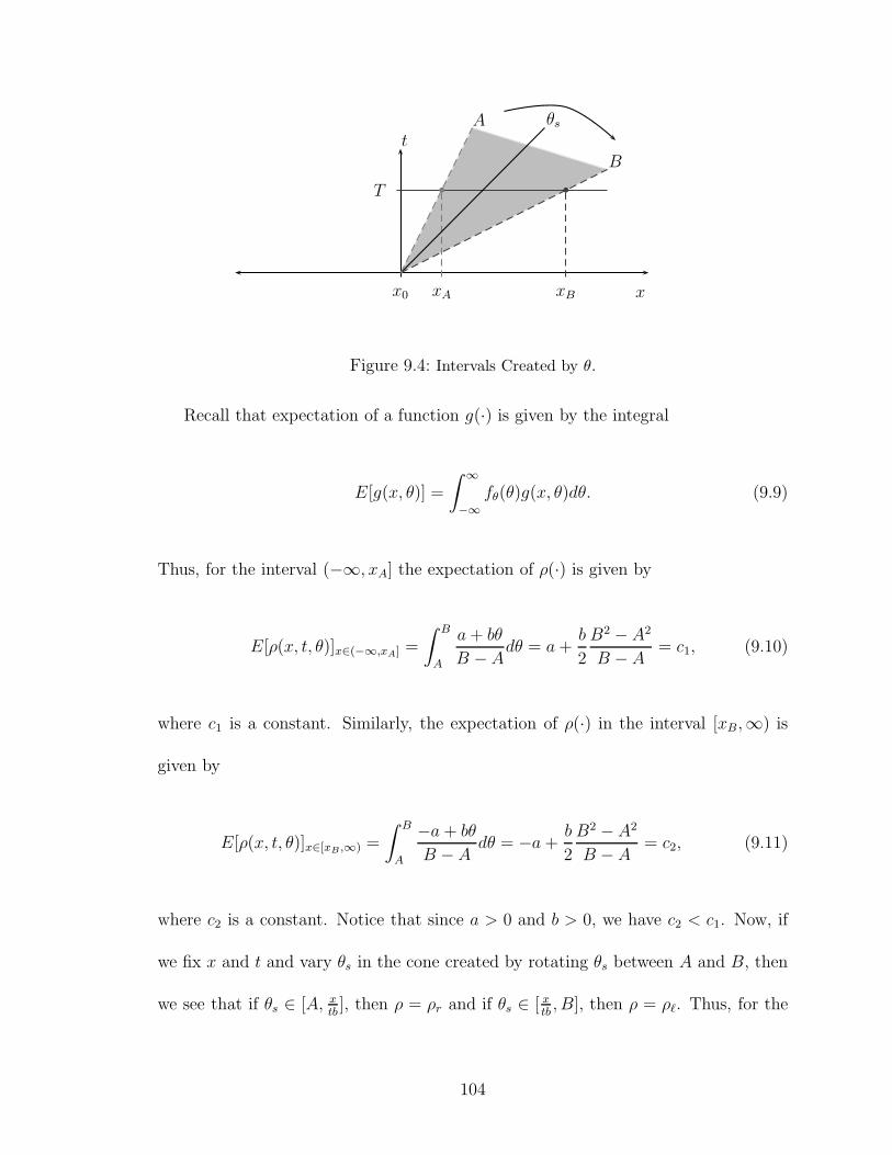
x

t

x0

T

xBxA

θs

B

A

Figure 9.4: Intervals Created by θ.

Recall that expectation of a function g(·) is given by the integral

E[g(x, θ)] =

∫ ∞

−∞

fθ(θ)g(x, θ)dθ. (9.9)

Thus, for the interval (−∞, xA] the expectation of ρ(·) is given by

E[ρ(x, t, θ)]x∈(−∞,xA] =

∫ B

A

a+ bθ

B −Adθ = a+

b

2

B2 − A2

B − A= c1, (9.10)

where c1 is a constant. Similarly, the expectation of ρ(·) in the interval [xB,∞) is

given by

E[ρ(x, t, θ)]x∈[xB ,∞) =

∫ B

A

−a + bθ

B − Adθ = −a + b

2

B2 − A2

B − A= c2, (9.11)

where c2 is a constant. Notice that since a > 0 and b > 0, we have c2 < c1. Now, if

we fix x and t and vary θs in the cone created by rotating θs between A and B, then

we see that if θs ∈ [A, xtb], then ρ = ρr and if θs ∈ [ x

tb, B], then ρ = ρℓ. Thus, for the

104

interval [xA, xB], the expectation is given by

E[ρ(x, t, θ)]x∈[xA,xB] =

∫ x/(tb)

A

−a+ bθ

B − Adθ +

∫ B

x/(tb)

a + bθ

B − Adθ

=1

B − A

(

[

−aθ + b

2θ2]x/(tb)

A

+

[

aθ +b

2θ2]B

x/(tb)

)

(9.12)

=1

B − A

[

−2ax

tb+ a(A+B) +

b

2(B2 − A2)

]

.

Notice, that the expectation E[ρ(x, t, θ)] where x ∈ [xA, xB] is a linear relation de-

pendent on x and t. To verify that the expectations are consistent with one another

at the end points, consider xB = tbB. Plug x = xB into equation (9.13). We get

E[ρ(xB , t, θ)]x∈[xA,xB] =1

B − A

[

2axBtb

− a(A+B) +b

2(B2 −A2)

]

=1

B − A

[

−2atbB

tb+ a(A +B) +

b

2(B2 − A2)

]

=1

B − A

[

−2aB + a(A+B) +b

2(B2 −A2)

]

(9.13)

=1

B − A

[

−a(B − A) +b

2(B2 − A2)

]

=

[

−a + b

2

(B2 −A2)

B −A

]

= c2

105

Now, consider xA = tbA. Plug x = xA into equation (9.13). We get

E[ρ(xA, t, θ)]x∈[xA,xB] =1

B − A

[

2axAtb

− a(A +B)− b

2(B2 − A2)

]

=1

B − A

[

−2atbA

tb+ a(A+B) +

b

2(B2 −A2)

]

=1

B − A

[

−2aA + a(A+B) +b

2(B2 − A2)

]

(9.14)

=1

B − A

[

a(B −A) +b

2(B2 −A2)

]

=

[

a+b

2

(B2 − A2)

B − A

]

= c1

Figure (9.5) shows the expectation of ρ(x, t, θ) for fixed t in the three regions. As

expected the expectation is a continuous function, constant in the intervals (−∞, xA]

and [xB,∞) and linear in the region [xA, xB].

E[ρ(x, t, θ)]

E[ρ(x, t, θ)]x∈(−∞,xA]

xA xB

E[ρ(x, t, θ)]x∈[xB ,∞)

E[ρ(x, t, θ)]x∈[xA,xB]

Figure 9.5: Expectation of ρ(x, t, θ).

Now, we consider the second moment. Recall the second moment of a function

106

g(·) is given by the integral

E[g2(x, θ)] =

∫ ∞

−∞

fθ(θ)g2(x, θ)dθ. (9.15)

In order to calculate the second moment of ρ(·) we must consider the behavior in the

following intervals: (−∞, xA], [xA, xB] and [xB,∞) where xA corresponds to θs = A

and xB corresponds to θs = B. For the interval (−∞, xA], the second moment of ρ(·)

is given by

E[ρ2(x, t, θ)]x∈(−∞,xA] =

∫ B

A

(a+ bθ)2

B − Adθ

= a2 +1

B −A

[

ab(B2 − A2) +b2

3(B3 −A3)

]

= c3, (9.16)

where c3 is constant. Similarly, the second moment of ρ(·) in the interval [xB,∞) is

given by

E[ρ2(x, t, θ)]x∈(xB ,∞] =

∫ B

A

(−a + bθ)2

B − Adθ

= a2 − 1

B −A

[

ab(B2 −A2)− b2

3(B3 − A3)

]

= c4, (9.17)

where c4 is a constant. Notice that a > 0 and b > 0, we have c4 < c3. Similar to

the calculation of expectation, if we fix x and t and vary θs in the cone created by

rotating θs between A and B, then we see that if θs ∈ [A, xtb], then ρ = ρr and if

θs ∈ [ xtb, B], then ρ = ρl. Thus, for the interval [xA, xB], the second moment is given

107

by

E[ρ2(x, t, θ)]x∈[xA,xB] =

∫ x/(tb)

A

(−a + bθ)2

B − Adθ +

∫ B

x/(tb)

(a+ bθ)2

B − Adθ (9.18)

=1

B −A

(

[

b2

3θ3 − abθ2 + a2θ

]x/(tb)

A

+

[

a2θ + abθ2 +b2

3θ3]B

x/(tb)

)

= a2 +1

B − A

[

−2ab( x

tb

)2

+b2

3(B3 −A3) + ab(A2 +B2)

]

.

To verify that the second moments in the intervals are consistent with one another

at the end points, consider xB = tbB. Plug x = xB into equation (9.19).

E[ρ2(xB, t, θ)]x∈[xA,xB] = a2 +1

B − A

[

−2ab(xBtb

)2

+b2

3(B3 − A3) + ab(A2 +B2)

]

= a2 +1

B − A

[

−2abB2 +b2

3(B3 − A3) + ab(A2 +B2)

]

(9.19)

= a2 − 1

B −A

[

ab(B2 −A2)− b2

3(B3 − A3)

]

= c4.

Now, consider xA = tbA. Plug x = xA into equation (9.19).

E[ρ2(xA, t, θ)]x∈[xA,xB] = a2 +1

B − A

[

−2ab(xAtb

)2

+b2

3(B3 −A3) + ab(A2 +B2)

]

= a2 +1

B − A

[

−2abA2 +b2

3(B3 − A3) + ab(A2 +B2)

]

(9.20)

= a2 +1

B − A

[

ab(B2 − A2) +b2

3(B3 − A3)

]

= c3.

Figure (9.6) shows the second moment of ρ(x, t, θ) for fixed t in the three re-

108

gions. As expected the expectation is a continuous function, constant in the intervals

(−∞, xA] and [xB ,∞) and linear in the region [xA, xB].

E[ρ2(x, t, θ)]

E[ρ2(x, t, θ)]x∈(−∞,xA]

xA xB

E[ρ2(x, t, θ)]x∈[xB,∞)

E[ρ2(x, t, θ)]x∈[xA,xB]

Figure 9.6: Second Moment of ρ(x, t, θ).

9.3 Summary

In this chapter we have provided the theory for how to propagate uncertainty in

the initial condition through Burgers’ equation. In future work, a conservation form

will be developed for this method of propagating uncertainty in the initial condition.

The work presented here is original, and thus, is a contribution.

109

CHAPTER 10

NUMERICAL SOLUTION TO THE LIOUVILLE EQUATION

In this chapter we apply the Liouville equation to examples of ODEs including various

linear ODEs. The resulting Liouville equations that we solve are constant advection

and variable advection equations. We used MATLAB to numerically solve the Li-

ouville equation. The numerical method we use is the Godunov method, which is a

common method for numerically solving hyperbolic partial differential equations like

the Liouville equation. The Godunov method utilizes a Riemann solver. The results

are presented in this chapter and the code is presented in Appendix A.

10.1 Simulations for Constant Advection Equation

The first example of an ODE that we explore is of the form

x = −5, (10.1)

with initial condition given as a normally distributed random variable. The pdf for

the random variable corresponding to the initial condition was taken to be

uX0(x) =1√5πe

−x

5 . (10.2)

The LE then becomes

∂u

∂t+

∂

∂x[−5u] = 0. (10.3)

Figure (10.1) confirms that as the system evolves the geometry of the pdf remains

the same but it advects or drifts. The diffusion that is present in figure (10.1) is a

110

−10 −9 −8 −7 −6 −5 −4 −3 −2 −1 0 1 2 3 4 50

0.05

0.1

0.15

0.2

0.25

0.3

0.35

0.4Constant Advection Equation

x

pdf

t=1t=1700t=2500t=3750

Figure 10.1: Constant Advection Equation Results

result of the numerical method and not a result of the application of the LE to the

problem of uncertainty propagation.

10.2 Simulations for Variable Advection Equation

The second example of an ODE that we explore is of the form

x = −5x, (10.4)

with initial condition given as a normally distributed random variable. The pdf for

the random variable corresponding to the initial condition was taken to be

uX0(x) =1√5πe

−x

5 . (10.5)

111

−10 −9 −8 −7 −6 −5 −4 −3 −2 −1 0 1 2 3 4 50

0.05

0.1

0.15

0.2

0.25

0.3

0.35

0.4

prob

abili

ty d

ensi

ty

x

(a) Time 1: Initial

−10 −9 −8 −7 −6 −5 −4 −3 −2 −1 0 1 2 3 4 50

0.05

0.1

0.15

0.2

0.25

0.3

0.35

0.4

prob

abili

ty d

ensi

tyx

(b) Time 2

−10 −9 −8 −7 −6 −5 −4 −3 −2 −1 0 1 2 3 4 50

0.05

0.1

0.15

0.2

0.25

0.3

0.35

0.4

prob

abili

ty d

ensi

ty

x

(c) Time 3

−10 −9 −8 −7 −6 −5 −4 −3 −2 −1 0 1 2 3 4 50

0.05

0.1

0.15

0.2

0.25

0.3

0.35

0.4

prob

abili

ty d

ensi

ty

x

(d) Time 4

Figure 10.2: Uncertainty Propagation in ODE y′ = −5

112

The LE then becomes

∂u

∂t+

∂

∂x[−5xu] = 0. (10.6)

−5 −4 −3 −2 −1 0 1 2 3 4 50

1

2

3

4

5

6

7Variable Advection Equation

x

pdf

t=1t=1700t=2500t=3750

Figure 10.3: Variable Advection Equation Results

We expect that with a stable ODE such as the one chosen for this example, we

should observe the geometry of the pdf approach that of a Dirac delta distribution

centered around the mean. Figures(10.4) and (10.2) confirm that as the system

evolves the geometry of the pdf approaches that of the Dirac delta distribution.

10.3 Summary

In this chapter we present several examples of propagation of uncertainty through

ODEs. MATLAB code was written to solve the LE which is the method for propaga-

tion of uncertainty through ODEs. Plots of the pdf as it evolves have been included.

113

−20 −15 −10 −5 0 5 10 15 200

0.5

1

1.5

2

2.5

3

3.5

4

prob

abili

ty d

ensi

ty

x

(a) Time 1: Initial

−5 −4 −3 −2 −1 0 1 2 3 4 50

1

2

3

4

5

6

7

prob

abili

ty d

ensi

tyx

(b) Time 2

−5 −4 −3 −2 −1 0 1 2 3 4 50

1

2

3

4

5

6

7

prob

abili

ty d

ensi

ty

x

(c) Time 3

−5 −4 −3 −2 −1 0 1 2 3 4 50

1

2

3

4

5

6

7

prob

abili

ty d

ensi

ty

x

(d) Time 4

Figure 10.4: Uncertainty Propagation in ODE y′ = −5x

114

CHAPTER 11

NUMERICAL SOLUTION FOR UNCERTAINTY PROPAGATION IN FDES

In this chapter we apply the theory of functions of random variables to basic finite

difference equations. Taking simple finite difference equations, we use MATLAB to

propagate the uncertainty from the initial condition.

11.1 Simulations

Consider a FDE of the form

x[k + 1] = ax[k] + b (11.1)

with an initial condition x[0] = X0 given as a normally distributed random variable.

Using functions of random variables, code was written in MATLAB to simulate the

propagation of uncertainty in a system of this type.

11.1.1 FDE Example One

The example presented in this section is uncertainty propagation through the FDE

given by

x[k + 1] = 0.5x[k] (11.2)

with the pdf of the initial condition given by

uX0(x) =2

25e

−x2

50 . (11.3)

The code used to propagate the initial uncertainty is given in Appendix A.

115

−20 −15 −10 −5 0 5 10 15 200

0.1

0.2

0.3

0.4

0.5

0.6

0.7

xpr

obab

ility

den

sity

t=1t=2t=3t=4

Figure 11.1: Uncertainty Propagation in FDE x[k + 1] = 0.5x[k]

We can see from figure (11.1) that the pdf is approaching the Dirac delta distri-

bution since the constant a = 0.5 is less than one. The mean of the pdf remains at

zero due to the fact that there is no ’drift’ term associated with the FDE.

11.1.2 FDE Example Two

The example presented in this section uncertainty propagation through the FDE

given by

x[k + 1] = 2x[k] + 6 (11.4)

with the pdf of the initial condition given by

uX0(x) =2

25e

−x2

50 . (11.5)

The code used to propagate the initial uncertainty is given in Appendix A.

We can see from figure (11.2) that the pdf is approaching is diffusing since the

constant a = 2 is greater than one. The mean of the pdf shifting due to the fact that

116

−150 −100 −50 0 50 100 150 200 2500

0.01

0.02

0.03

0.04

0.05

0.06

0.07

0.08

x

prob

abili

ty d

ensi

ty

t=1t=2t=3t=4

Figure 11.2: Uncertainty Propagation in FDE x[k + 1] = 2x[k] + 6

there is a ’drift’ term associated with the FDE, i.e. b = 6.

The examples presented in this chapter provide an basic understanding of how we

propagate uncertainty through FDEs using functions of random variables.

11.2 Summary

In this chapter we present several examples of propagation of uncertainty through

FDEs. MATLAB code was written to simulate the propagation of uncertainty from

the initial condition in FDEs. Plots of the pdf as it evolves have been included.

117

CHAPTER 12

CONCLUSIONS

A fundamental principle of science is that no real measurement or model is infinitely

precise. It has an inherent degree of uncertainty that we must accept and learn to

process and incorporate into our models and our designs. The utility of a model is

determined by its predictive ability. To consider uncertainty in the modeling pro-

cess allows for increased model utility. Uncertainty can be in the model parameters,

boundary conditions, initial conditions and the dynamics themselves. The work pre-

sented in this thesis attempts to address the issue of uncertainty modeling in dynamic

systems. In particular, we present a conservation based method of propagating un-

certainty in the initial condition through the system given that the initial condition

is defined within some probability structure. The conservation based method for un-

certainty propagation follows directly from the global conservation law of probability,

∫

Ω

uX(x, t)dP = 1, (12.1)

which is a fundamental principle in probability theory. It allows for the probability

function to be a measurable function and allows for the theory developed in this

thesis to be consistent with the probability structure on the problem of uncertainty

propagation from the initial condition. The mathematical integrity of the problem of

uncertainty propagation heavily depends on this.

The main idea presented in this thesis is that given an initial state space defined

on a probability structure, system dynamics, and an evolution operator that maps

the initial state space to a state space at time t > 0, we define a probability structure

118

on the state at time t > 0 such that the evolution operator is measure preserving.

This idea is the fundamental concept which is central to the theory of conservation

based uncertainty propagation in the dynamic systems presented in this thesis.

12.1 Ordinary Differential Equations

The method for propagating uncertainty in the initial condition through ODEs

and systems of ODEs is the Liouville equation. The work in this thesis presents

the derivation of the Liouville Equation and its solution. The Liouville equation is

derived based on conservation of probability mass and is consistent with preserving the

probability measure. The Liouville equation as derived for propagation of uncertainty

in ODEs is a semilinear hyperbolic partial differential equation, and thus, there are

only a few cases in which we can solve the Liouville equation analytically. Numerical

method must be employed to propagate uncertainty in ODEs in a practice.

12.2 Finite Difference Equations

FDEs are the discrete time analog to ODEs. The method for propagating uncer-

tainty in the initial condition in FDEs is through the theory of functions of random

variables. The work in this thesis presents the development of the theory of functions

of random variables are it pertains to propagation of uncertainty in FDEs. Using

functions of random variables we are able to preserve the probability measure defined

in the probability space given as part of the initial condition through defining the

state of the system as a random variable and considering the dynamics to be simply a

function of random variable(s). Thus, this method is consistent with the conservation

119

principle.

12.3 Differential Inequalities and Inclusions

Differential inequalities and inclusions are the most abstract mathematical model

under consideration. In this thesis we present a method for uncertainty propagation

only in a small class of differential inclusions. The method for propagation is through

defining a probability structure on the initial set of possible values the dynamics can

take. Over each interval in the initial set, we define a scaled uniform density. The

sum the sum of these functions over the entire initial set is a density function with

the appropriate properties. For each interval, we propagate this initial distribution

according to the dynamics by taking the supremum of the upper bound function over

the interval and the infimum of the lower bound function over all possible values in

the interval thereby creating a new interval from these values. The distribution over

the initial interval is uniformly spread out over the new interval. This method of

uncertainty propagation is also conservation based and is consistent with our defined

probability structure.

12.4 Stochastic Differential Equations

The method for propagating uncertainty in the initial condition in SDEs is through

the Fokker-Planck equation. The work in this thesis presents the derivation of the

FPE and how it is used to solve for the pdf of the states of a system of SDEs at future

time. We also show that the FPE can be written in conservation form. The FPE is

a partial differential equation, and thus, numerical methods must be use to solve for

120

the pdf at future times. It is very interesting, mathematically speaking, to note that

uncertainty propagation from the initial condition in a SDE, which is a model that

accounts for randomness, can be converted to a partial differential equation which

is deterministic. This means an inherently stochastic problem becomes deterministic

when the appropriate probability structure is defined.

12.5 Markov Chains

Markov chains are an interesting class of dynamics systems which are memoryless.

Future states only depend on the current state of a system. Thus, for uncertainty

propagation, they are interesting to study. In this thesis we review what Markov

property and what constitutes a Markov chain. We also show that the problem of

uncertainty propagation in Markov chains can be solved using probabilistic infer-

ence. This means that by applying the transition probabilities iteratively, posterior

distributions for the states of the system can be determined.

12.6 Uncertainty Propagation in Burgers’ Equation

Burgers’ equation is a nonlinear hyperbolic partial differential equation. In this

thesis, we present a method for propagating uncertainty in the initial condition

through Burgers’ equation. We assume that the initial data is piecewise constant

function with a random parameter that renders the initial data to be stochastic. We

also assume the the random parameter is uniformly distributed. The method pre-

sented uses only the dynamics of the system and the initial data. Propagation of

uncertainty is done using the characteristics of the system and evaluating the expec-

121

tation of the velocity variable.

12.7 Future Work

The work presented in this thesis is only a scratch in the surface. The range of

the term dynamic systems is very broad and this study covers only a small subset

of what we call dynamic systems. In the future, we hope to expand this study to

include a study of a more general and abstract set of dynamic systems and a study

of qualitative properties such as stability analysis and the conditions under which

the problems become well posed. In addition, we hope to apply some of the results

presented to various practical systems such as transportation networks and financial

markets.

122

APPENDIX A

MATLAB CODE

A.1 MATLAB Code for Liouville Equation

This section of the appendix includes the MATLAB code used to propagate un-

certainty through ODEs.

A.1.1 Constant Advection Equation

a = -20; b = 20; T = 1; M = 500; rhom = 0.2;

n = 100; drho = rhom/n; rho = 0:drho:rhom;

h = (b-a) / M;

xticks = transpose(a+h/2:h:b-h/2);frho = fluxadvec(xticks);

[qmax,s] = max(frho);

rhostar = rho(s);

% CFL Condition

lambda = max(abs(frho(2:n)-frho(1:n-1)))/drho;

ka = 0.5 * h / lambda;

N = ceil(T/ka) ;

k = T / N;

% Initialise:

U = zeros(M,N+1);

U(:,1) = initialadvec(xticks);

123

figure(1);

plot(xticks,U(:,1),’k’,’LineWidth’,2)

axis([a b 0 4])

ylabel(’probability density’)

xlabel(’x’)

% Algorithm

for j=1:N

rhol = U(1:M-1,j);

rhor = U(2:M,j);

qval=-5*U(:,j);

ql = qval(1:M-1);

qr = qval(2:M);

case1 = rhol <= rhor;

case2 = rhol > rhostar & rhostar > rhor;

case3 = not(case1 | case2);

Q = case1 .* min(ql,qr) + case2 * qmax + case3 .* max(ql,qr);

% Specifying Boundary Flows

d=transpose(fluxadvec(initialadvec(a)));

Q = [-5*initialadvec(a); Q; qval(M)];

U(:,j+1)=U(:,j) + (k/h) * (Q(1:M) - Q(2:M+1));

end

124

% initialadvec.m

function init=initialadvec(x)

init=1/4 * exp(-x.^2/5);

% fluxadvec.m

function fl=fluxadvec(rho)

fl = -5*rho;

% fluxadvec2.m

function fl=fluxadvec2(u)

for i = 1:500

fl(i)=-5*u(i);

end

A.1.2 Variable Advection Equation

%System Variables

%Domain: [a,b]

a = -20;

b = 20;

%Stopping Time = 1

T = 1;

M = 500;

%x-vector and dx

h = (b-a) / M;

xticks = transpose(a+h/2:h:b-h/2);

125

%Initial Condition

u0=initialadvec(xticks);

%Determine rho*

[umax,m]=max(u0);

du=umax/n;

frho = fluxadvec(xticks);

[qmax,s] = max(frho);

rhostar = xticks(s);

% CFL Condition

lambda = max(abs(frho(2:n)-frho(1:n-1)))/du;

ka = 0.5 * h / lambda;

N = ceil(T/ka) ;

k = T / N;

% Initialize:

U = zeros(M,N+1);

U(:,1) = initialadvec(xticks);

% Algorithm

for j=1:N

rhol = U(1:M-1,j);

rhor = U(2:M,j);

qval = transpose(fluxadvec2(xticks,U(:,j)));

ql = qval(1:M-1);

qr = qval(2:M);

126

case1 = rhol <= rhor;

case2 = rhol > rhostar & rhostar > rhor;

case3 = not(case1 | case2);

Q = case1 .* min(ql,qr) + case2 * qmax + case3 .* max(ql,qr);

% Specifying Boundary Flows

d=transpose(fluxadvec(initialadvec(a)));

Q = [d*U(1,j); Q; qval(M)];

%Determine U at t=j+1

U(:,j+1)=U(:,j) + (k/h) * (Q(1:M) - Q(2:M+1));

end

% fluxvaradvec.m

function fl=fluxvaradvec(x,u)

fl1 = -5*x;

for i = 1:500

fl(i)=fl1(i)*u(i);

end

A.2 MATLAB Code for Finite Difference Equations

The code in this section is for the simulation of uncertainty propagation in FDEs.

A.2.1 FDE Example 1

%Initialize Variables

a=0.5; b= 0; N=500;M=100;

127

y1=-20; y2=20; dy = (y2-y1)/N;

y= transpose(y1+dy/2:dy:y2-dy/2);

fx= zeros(N,M+1);

fx(:,1) = 0.08 * exp(-y.^2/50);

yold1=y1;

yold2=y2;

yv(:,1)=y;

%Algorithm

for j = 1: 4

yend1=yold1*a+b;

yend2=yold2*a+b;

delta=(yend2-yend1)/N;

yvec=transpose(yend1+delta/2:delta:yend2-delta/2);

yv(:,j+1)=yvec;

sum = 0;

for m = 1: j

sum = sum +b/a^m;

end

for i = 1:N

ynew(i) = yvec(i)/a^(j)-sum;

end

f = 0.08 * exp(-ynew.^2/50);

fx(:,j+1)=(1/(abs(a))^(j))*f;

128

yold1=yend1;

yold2=yend2;

end

%Plot

figure(1);

plot(yv(:,1),fx(:,1),yv(:,2),fx(:,2),yv(:,3)...

,fx(:,3),yv(:,4),fx(:,4),’k’,’LineWidth’,2)

grid on

legend(’t=1’,’t=2’,’t=3’, ’t=4’)


xlabel(’x’)

A.2.2 FDE Example 2

%Initialize Variables

a=2; b= 6; N=500;M=100;

y1=-20; y2=20; dy = (y2-y1)/N;

y= transpose(y1+dy/2:dy:y2-dy/2);

fx= zeros(N,M+1);

fx(:,1) = 0.08 * exp(-y.^2/50);

yold1=y1;

yold2=y2;

yv(:,1)=y;

%Algorithm

129

for j = 1: 4

yend1=yold1*a+b;

yend2=yold2*a+b;

delta=(yend2-yend1)/N;

yvec=transpose(yend1+delta/2:delta:yend2-delta/2);

yv(:,j+1)=yvec;

sum = 0;

for m = 1: j

sum = sum +b/a^m;

end

for i = 1:N

ynew(i) = yvec(i)/a^(j)-sum;

end

f = 0.08 * exp(-ynew.^2/50);

fx(:,j+1)=(1/(abs(a))^(j))*f;

yold1=yend1;

yold2=yend2;

end

%Plot

figure(1);

plot(yv(:,1),fx(:,1),yv(:,2),fx(:,2),yv(:,3)...

,fx(:,3),yv(:,4),fx(:,4),’k’,’LineWidth’,2)

grid on

130

legend(’t=1’,’t=2’,’t=3’, ’t=4’)


xlabel(’x’)

131

BIBLIOGRAPHY

[1] George L. Shackle. Decision, order, and time in human affairs. Cambridge

University Press, 1961.

[2] Frederic Y. Bois and Cheikh T. Diack. Recent Advances in Quantitative Methods

in Cancer and Human Health Risk Assessment, chapter 15, pages 255–266. Wiley,

2005.

[3] Athanasios Papoulis. Probability, Random Variables and Stochastic Processes.

McGraw-Hill Book Company, 1965.

[4] Lawrence C Evans. An Introduction to Stochastic Differential Equations Version

1.2, 2008.

[5] Hisa Tanaka. Quick derivation of fokker-planck equation. [email protected],

Nov. 2005.

[6] Alex Bielajew. Monte carlo modeling in external electronbeam radiotherapy-why

leave it to chance? National Research Council, Ottawa Canada.

[7] Norbert Wiener. The homogeneous chaos. American Journal of Mathematics,

60(4):897–936, 1938.

[8] Adrian Sandu, Corina Sandu, and Mehdi Ahmadian. Modeling multibody sys-

tems with uncertainties. part 1: Theoretical and computational aspects. Multi-

body System Dynamics, 15(4):369–391, May 2006.

132

[9] Teems E. Lovett, Ferdinanda Ponci, and Antonello Monti. A polynomial chaos

approach to measurement uncertainty. IEEE Transactions on Intrumentation

and Measurement, 55(3):723–736, June 2006.

[10] Teems E. Lovett, Antonello Monti, and Ferdinanda Ponci. Automatic synthesis

of uncertain models from linear circuit simulation: A polynomial chaos theory

approach. Simulation Modelling Practice and Theory, 16:796–816, 2008.

[11] Per Pettersson, Gianluca Iaccarino, and Jan Nordstrom. Numerical analysis of

the burger’s equation in the presence of uncertainty. Journal of Computational

Physics, 2009.

[12] R. H. Cameron and W. T. Martin. The orthogonal development of non-linear

functionals in series of fourier-hermite functionals. Annals of Mathematics,

48(2):385–392, April 1946.

[13] Dongbin Xiu and George Em Karniadakis. The wiener-askey polynomial chaos

for stochastic differential equations. SIAM Journal on Scientific Computing,

24(2):619–644, 2002.

[14] Pradya Prempraneerach. Uncertainty Analysis in Shipboard Integrated Power

System using Multi-Element Polynomial Chaos. PhD thesis, Massachusetts In-

stitute of Technology, 2007.

[15] Willian A. Link and Richard J. Barker. Bayesian Inference with Ecological Ap-

plications. Elsevier, 2010.

133

[16] S.F. Su and C.S.G. Lee. Uncertainty manipulation and propagation and verifica-

tion of applicability of actions in assembly tasks. In Proceedings of the 1991 IEEE

International Conference on Robotics and Automation, Sacramento, California,

April 1991.

[17] L.A.F. Fernandes, M. Oliveira, and R. da Silva. Uncertainty propagation: Avoid-

ing the expensive sampling process for real-time image-based measurements.

Journal of Computational Statistics and Data Analysis, 52:3852–3876, 2007.

[18] B. Ruggeri. Chemicals exposure: Scoring procedure and uncertainty propagation

in scenario selection for risk analysis. Chemosphere, 77:330–338, 2009.

[19] A. Abusam, K.J. Keesman, and G. van Straten. Forward and backward un-

certainty propagation: an oxidation ditch modeling example. Water Research,

37:429–435, 2003.

[20] P. Baraldi and E. Zio. A combined monte carlo and possibilistic approach to

uncertianty propagation in event tree analysis. Risk Analysis, 28:1309–1325,

2008.

[21] S. Blasone, A. Vrugt, H. Madsen, D. Rosbjerg, B. Robinson, and G. Zyvoloski.

Generalized likelihood uncertainty estimation (glue) using adaptive markov chain

monte carlo sampling. Advances in Water Resources, 31:630–648, 2008.

[22] L. Cristaldi, M. Faifer, and F. Ponci. Uncertainty propagation in diagnostic

systems based on soft computing techniques. In Proceedings of International

134

Workshop on Advanced Methods for Uncertianty Estimation in Measurement,

Sardagna, Trento, Italy, July 2007.

[23] Martin Ehrendorfer. The liouville equation and atomospheric predictability. In

Predictability of Weather and Climate, pages 59–98. Cambridge University Press,

2006.

[24] S.H. Lee and W. Chen. A comparative study of uncertainty propgation meth-

ods for black-box type problems. Structural and Multidisciplinary Optimization,

37(3):239–253, January 2009.

[25] T. Lee, M. Leok, and N.H. McClamroch. Global symplectic uncertainty prop-

agation on so(3). In Proceedings of the 47th IEEE Conference on Decision and

Control, Cancun, Mexico, December 2008.

[26] L. Mari. A computational system for uncertainty propagation of measurement

results. Measurement, 42:844–855, 2009.

[27] A. Mencattini, S. Marcello, and R. Lojacono. On generalized t-norm for the rep-

resentation of uncertianty propagation in statistically correlated measurements

by means of fuzzy variables. In Proceedings of International Workshop on Ad-

vanced Methods for Uncertianty Estimation in Measurement, Sardagna, Trento,

Italy, December 2007.

[28] A. Sandu, C. Sandu, and M. Ahmadian. Modeling multibody systems with uncer-

tainties. part 2: Numerical applications. Multibody System Dynamics, 15(4):241–

262, May 2006.

135

[29] G. Terejanu, P. Singla, T. Singh, and P. Scott. Uncertianty propagation for

nonlinear dynamic systems using gaussian mixture models. Journal of Guidance,

Control and Dynamics, 31:1623–1633, 2008.

[30] Anthony N. Michel, Kaining Wang, and Bo Hu. Qualitative Theory of Dynamical

Systems: The Role of Stability Preserving Mappings. Marcel Dekker, Inc., 2nd

edition, 2001.

[31] Bernt Oksendal. Stochastic Differential Equations. Springer-Verlag, 3 edition,

1992.

[32] Zdzislaw Brezezniak and Tomasz Zastawniak. Basic Stochastic Processes.

Springer, 1999.

[33] Paul G. Hoel, Sidney C. Port, and Charles J. Stone. Introduction to Stochastic

Processes. Houghton Mifflin Company, 1972.

[34] Richard Bronson and Gabriel B. Costa. Schaum’s Outline of Differential Equa-

tions. McGraw-Hill Book Company, 2006.

[35] Martin Ehrendorfer. The Liouville Equation and Its Potential Usefulness for the

Prediction of Forecast Skill. Part I: Theory. Monthly Weather Review, 122:703–

713, May 1993.

[36] Martin Ehrendorfer. The Liouville Equation and Its Potential Usefulness for

the Prediction of Forecast Skill. Part II: Applications. Monthly Weather Review,

122:714–728, May 1993.

136

[37] Patricia Mellodge and Pushkin Kachroo. Model Abstraction in Dynamical Sys-

tems: Application to Mobile Robot Control. Lecture Notes In Control and Infor-

mation Sciences. Springer, 2008.

[38] David Richard Wolf. Information and correlation in statistical mechanical sys-

tems. University of Leeds, 1996.

[39] Jean-Pierre Aubin. Set-Valued Analysis. Birkhauser, 1990.

[40] Y.A. Rozanov. Probability Theory: A Concise Course. Dover Publications, 1969.

[41] Randall J. LeVeque. Numerical Methods for Conservation Laws. Birkhauser,

1992.

[42] Randall J. LeVeque. Finite Volume Methods for Hyperbolic Problems. Cambridge

University Press, 1995.

137

VITA

Graduate CollegeUniversity of Nevada, Las Vegas

Lillian J. Ratliff

Degrees:Bachelors of Science, Electrical Engineering, 2008University of Nevada, Las Vegas

Bachelors of Science, Mathematics, 2008University of Nevada, Las Vegas

Special Honors and Awards:National Science Foundation Graduate Research Fellowship 2009

Publications:Cook, D. P., Y. Chen, L. J. Ratliff, and J. Ma. 2006. ’Numerical Modeling ofEM Pump Efficiency’. Proceedings of the 2006 American Society for MechanicalEngineering Annual Conference & Exposition.

Ratliff, L. and P. Kachroo. 2010. ’Validating Numerically Consistent MacroscopicTraffic Models Using Microscopic Data’. Transportation Research Board AnnualMeeting.

Thesis Title:Conservation Based Uncertainty Propagation in Dynamic Systems

Thesis Examination Committee:Chairperson, Pushkin Kachroo, Ph.D.Committee Member, Mehdi Ahmadian, Ph.D.Committee Member, Rama Venkat, Ph.D.Committee Member, Yahia Baghzouz, Ph.D.Graduate Faculty Representative, Mohammad Trabia, Ph.D.

138

Conservation based uncertainty propagation in dynamic systems

Documents

Transcript of Conservation based uncertainty propagation in dynamic systems