Conscientiousness, Extraversion, College Education, and … › journals › pdfs ›...
34
Online Appendix to “Conscientiousness, Extraversion, College Education, and Longevity of High-Ability Individuals” 1 Peter A. Savelyev June 13, 2020 1 Peter Savelyev is an Assistant Professor of Economics at The College of William & Mary and Research Affiliate at IZA. Email: [email protected]. This paper uses confidential Terman data provided by the Interuniversity Consortium for Political and Social Research, Ann Arbor, MI. The data can be obtained by filing a request directly with the CPSR. A version of this paper was presented to The Health Economics Workshop at the NBER Summer Institute; The Annual Meeting of the American Economic Association in Chicago; The European Economic Association and Econometric Society Annual European Meeting in Gothenburg, Sweden; The Health Economics Workshop and the Labor Group Seminar at the University of Chicago; Applied Microeconomics seminar at the Uni- versity of North Carolina; The Institute on Health Economics, Health Behaviors, and Disparities at Cornell University; Economics seminar of the Andrew Young School of Policy Studies, Georgia State University; Empirical Micro seminar of the University of Houston and Rice University; RAND Labor and Population Seminar in Santa-Monica; Departmental Seminar in Economics at Vanderbilt Uni- versity; the Applied Microeconomics Seminar at Vanderbilt Law School; The Quantitative Methods Brown Bag at the Department of Psychology and Human Development, Peabody College, Vanderbilt University; David Eccles School of Business research seminar, University of Utah; and the Upjohn Institute for Employment Research seminar. I thank participants of these meetings for useful sugges- tions and stimulating discussions. I am grateful to Gary Becker, Gabriella Conti, Miriam Gensowski, Mike Grossman, Tim Kautz, Don Kenkel, Adriana Lleras-Muney, Willard Manning, David Meltzer, R´ emi Piatek, Ben Williams, and especially Jim Heckman for productive comments. This version of the paper directly benefited from research assistance provided by Atticus Bolyard and Max Sacher and from proofreading by Xiaoyu (Nancy) Chen, Renee Garrow, Isabel Haber, and Eli Roth- leder. Work on this paper stretched over a decade, over which many RAs contributed to its development, namely Mihir Gandhi, Kai Hong, Hanchen Jiang, Adam Shriver, Ivana Stosic, and Kegon Tan. Sum- mer interns Keith Dent, Son Nghiem, John Spraul, and Cody Vaughn used previous versions of this paper to learn empirical skills and provided help. Peter Savelyev gratefully acknowledges research support from the College of William & Mary, Vanderbilt University, and the ERC at the University of Chicago. An early version of this research was supported by the Merck Quantitative Science Graduate Fellowship in Health Economics at the University of Chicago. The views expressed in this paper are those of the author and may not coincide with those of the funders.
Transcript of Conscientiousness, Extraversion, College Education, and … › journals › pdfs ›...

Online Appendix to “Conscientiousness,Extraversion, College Education, and Longevity
of High-Ability Individuals”1
Peter A. Savelyev
June 13, 2020
1Peter Savelyev is an Assistant Professor of Economics at The College of William & Mary andResearch Affiliate at IZA. Email: [email protected]. This paper uses confidential Terman dataprovided by the Interuniversity Consortium for Political and Social Research, Ann Arbor, MI. Thedata can be obtained by filing a request directly with the CPSR. A version of this paper was presentedto The Health Economics Workshop at the NBER Summer Institute; The Annual Meeting of theAmerican Economic Association in Chicago; The European Economic Association and EconometricSociety Annual European Meeting in Gothenburg, Sweden; The Health Economics Workshop andthe Labor Group Seminar at the University of Chicago; Applied Microeconomics seminar at the Uni-versity of North Carolina; The Institute on Health Economics, Health Behaviors, and Disparities atCornell University; Economics seminar of the Andrew Young School of Policy Studies, Georgia StateUniversity; Empirical Micro seminar of the University of Houston and Rice University; RAND Laborand Population Seminar in Santa-Monica; Departmental Seminar in Economics at Vanderbilt Uni-versity; the Applied Microeconomics Seminar at Vanderbilt Law School; The Quantitative MethodsBrown Bag at the Department of Psychology and Human Development, Peabody College, VanderbiltUniversity; David Eccles School of Business research seminar, University of Utah; and the UpjohnInstitute for Employment Research seminar. I thank participants of these meetings for useful sugges-tions and stimulating discussions. I am grateful to Gary Becker, Gabriella Conti, Miriam Gensowski,Mike Grossman, Tim Kautz, Don Kenkel, Adriana Lleras-Muney, Willard Manning, David Meltzer,Remi Piatek, Ben Williams, and especially Jim Heckman for productive comments. This version ofthe paper directly benefited from research assistance provided by Atticus Bolyard and Max Sacherand from proofreading by Xiaoyu (Nancy) Chen, Renee Garrow, Isabel Haber, and Eli Roth- leder.Work on this paper stretched over a decade, over which many RAs contributed to its development,namely Mihir Gandhi, Kai Hong, Hanchen Jiang, Adam Shriver, Ivana Stosic, and Kegon Tan. Sum-mer interns Keith Dent, Son Nghiem, John Spraul, and Cody Vaughn used previous versions of thispaper to learn empirical skills and provided help. Peter Savelyev gratefully acknowledges researchsupport from the College of William & Mary, Vanderbilt University, and the ERC at the University ofChicago. An early version of this research was supported by the Merck Quantitative Science GraduateFellowship in Health Economics at the University of Chicago. The views expressed in this paper arethose of the author and may not coincide with those of the funders.
Contents
A Exploratory and Confirmatory Factor Analysis of Noncognitive Measuresused in the Terman Study 2A.1 Establishing a Set of Childhood Noncognitive Measures that are Conceptually
Related to the Big Five . . . . . . . . . . . . . . . . . . . . . . . . . . . . . . . . 4A.2 Using Multiple Methods to Establish the Number of Latent Factors that Explain
the Given Set of Measures . . . . . . . . . . . . . . . . . . . . . . . . . . . . . . 4A.3 Using EFA to Finalize the Number of Factors and Identify Clusters of Measures
that Proxy these Factors . . . . . . . . . . . . . . . . . . . . . . . . . . . . . . . 5A.4 Using CFA to Confirm the EFA Results . . . . . . . . . . . . . . . . . . . . . . . 6A.5 Using the 1940 Data to Augment the 1922 Factors . . . . . . . . . . . . . . . . . 11
B Supplementary Figures and Tables 20
C The Likelihood Function 29
References 30

A Exploratory and Confirmatory Factor Analysis of Noncog-
nitive Measures used in the Terman Study
The aim of this section is to reanalyze noncognitive measures from the Terman data in order
to obtain five latent factors that are related to the contemporary Big Five traits: Openness,
Conscientiousness, Extraversion, Agreeableness, and Neuroticism.
According to John and Srivastava (1999), Openness describes the breadth, depth, originality,
and complexity of an individual’s mental and experimental life; Conscientiousness represents
“individual differences in the propensity to follow socially prescribed norms for impulse control,
to be task- and goal- directed, to be planful, to delay gratification, and to follow norms and
rules.” Alternatively, Conscientiousness can be described as the “propensity to be organized,
controlled, industrious, responsible, and conventional” (Roberts et al., 2009). Extraversion
implies an energetic approach to the social and material world and includes facets such as so-
ciability, activity, assertiveness, and positive emotionality. Agreeableness entails a prosocial and
communal orientation towards others and includes facets such as altruism, tender-mindedness,
trust, and modesty. Finally, Neuroticism contrasts emotional stability and even-temperedness
with negative emotionality, such as feeling anxious, nervous, sad, or tense.
Martin and Friedman (2000) show that strong links exist between personality measures used
in the Terman Data and the Big Five factors. However, previous authors documented neither
their exploratory nor their confirmatory factor analyses, which motivates research documented
in this appendix: finding the best specification for the latent factor model to be used in the
main paper.
As a result of the analysis presented below, I find that four of five factors defined in this
paper, childhood Conscientiousness and Extraversion as well as adult Agreeableness and Neu-
roticism, are defined in a similar way to factors that were empirically shown to be correlated
with the Big Five factors having the same names (Martin and Friedman, 2000). In particular,
Martin and Friedman show that Conscientiousness correlates well with Conscientiousness from
the Big Five taxonomy (correlation 0.55, and p-value below 0.001). The authors also demon-
2

strate a relationship between their Terman Sociability factor and Extraversion from the Big
Five taxonomy (with correlation 0.40, and p-value below 0.001). Extraversion in this paper is
defined similarly to Martin and Friedman’s Sociability, and, hence, should also be related to
Big Five Extraversion. Openness, as defined in this paper, was not empirically linked to the
Big Five, but it can be linked to the Big Five theoretically. To achieve the best model fit I
allow for cross-loadings (to be defined below), instead of using dedicated measures, which were
implemented in previous research. However, the effects of using cross-loadings on final model
results are minor.
The plan of the analysis described in this section is as follows:
1. Select a set of high-quality childhood personality measures from the Terman data so that
each measure from the set is conceptually related to the Big Five taxonomy.
2. Use multiple methods to establish the number of latent common factors that explain the
set of measures identified in (1). (These methods usually give several different answers to
be considered in the further analysis).
3. For each number of factors suggested by step (2), perform the exploratory factor analysis
(EFA) in order to establish the most reasonable number of factors; conditional on the most
reasonable number of latent factors, find clusters of measures that proxy the factors.
4. Use confirmatory factor analysis (CFA) to test model specifications suggested by EFA.
(As shown below, I establish measures that define childhood Conscientiousness, Openness,
and Extraversion).
5. Use the 1940 data to proxy those Big Five factors that are not represented in the 1922
data. (As described below, I add adulthood Agreeableness and Neuroticism.)
Each of the five steps in the above outline corresponds to one of the five sections below.
3

A.1 Establishing a Set of Childhood Noncognitive Measures that
are Conceptually Related to the Big Five
We want to find clusters of childhood noncognitive measures from 1922 that proxy Big Five
factors. Childhood measures are more valuable than adulthood ones for the purpose of this
paper, as they are measured before subjects start college. Additionally, the 1922 measures are
based on ratings from teachers and parents, which makes them more reliable than self-ratings
from 1940.
Based on theoretical definitions of the Big Five provided above, results from previous re-
search (Martin and Friedman, 2000; Martin et al., 2007), and advice from a leading psychol-
ogist1, I use the following childhood measures that are potentially related to the Big Five:
prudence and forethought, conscientiousness, truthfulness, desire to know, originality, general
intelligence, fondness for a large group, leadership, popularity with other children, cheerfulness
and optimism, permanency of moods, sensitiveness to approval and disapproval, freedom from
vanity and egoism, sympathy and tenderness, generosity and unselfishness.2 The next section
proceeds with establishing the number of latent common factors contained in these correlated
measures.
A.2 Using Multiple Methods to Establish the Number of Latent
Factors that Explain the Given Set of Measures
I use five alternative methods that establish the number of latent factors behind the measures
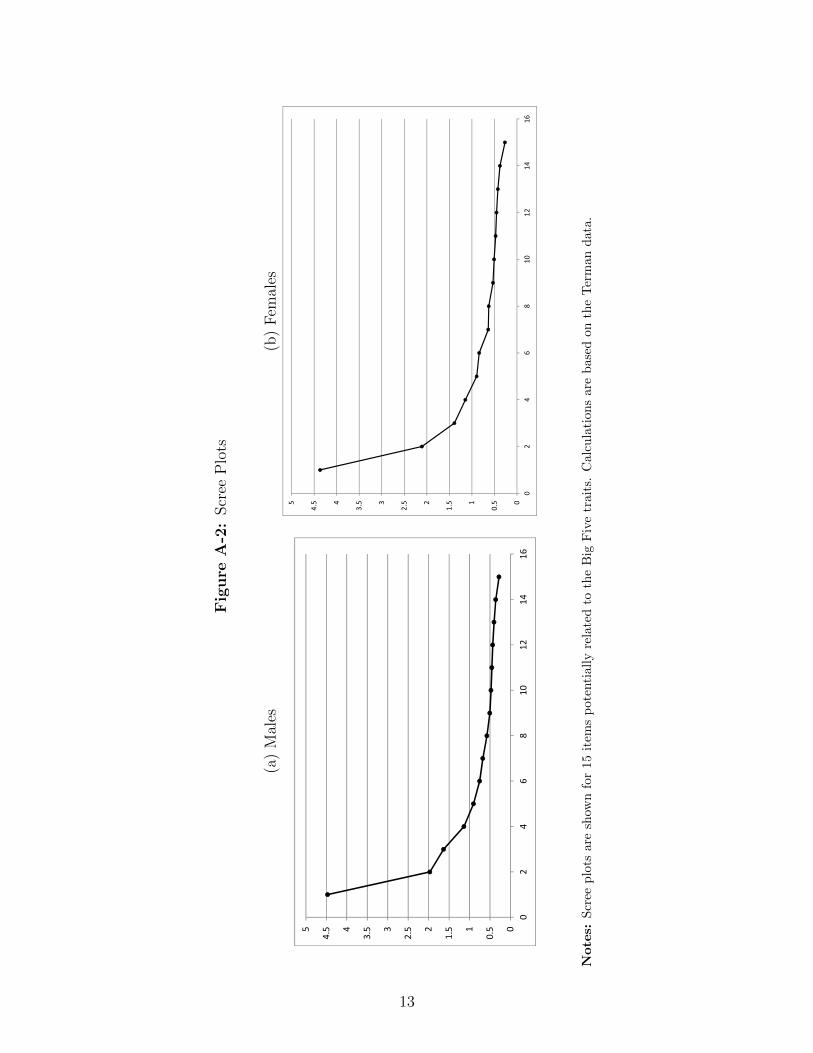
identified above. I use (1) the Guttman-Kaiser rule, (2) the scree test (e.g., Gorsuch, 1983),
(3) the Horn method (Gorsuch, 1983; Guttman, 1954; Horn, 1965; Kaiser, 1960, 1961), (4) the
Minap method (Velicer, 1976), and (5) the Onatski (2009) procedure. The “optimal number
of factors” represents an optimal balance between minimizing the number of common factors
1I am grateful to Angela Duckworth, a psychologist from the University of Pennsylvania, for a fruitfuldiscussion about conceptual links between Terman measures and the Big Five.
2See Figure A-1 for an example of a question measuring prudence. Teachers and parents had to put a crossanywhere on the line.
4

and maximizing the explained variance in the data. Viewing each measure as a separate factor
would explain 100% of variance but would also imply no dimensionality reduction and would
lead to problems such as high measurement error and multicollinearity. Instead, I want to
establish a small set of latent factors that explain a substantial share of variance, such that
adding an additional factor to this optimal set would have a negligible impact on explaining
the variance of measures.
Methods mentioned above differ by their approach to solving this optimization task, leading
to some variation in the recommended optimal number of factors (see also Heckman, Pinto,
and Savelyev (2013)). As Table A-1 shows, the optimal number of factors is estimated to be
2, 3, and 4.3 With the help of the EFA analysis in the next section I argue that 3 is the most
reasonable choice.
A.3 Using EFA to Finalize the Number of Factors and Identify Clus-
ters of Measures that Proxy these Factors
EFA can only be performed conditional on a given number of factors. When there are several
options (in our case 2, 3, or 4), it is standard to perform EFA conditional on each number,
compare results, weigh pros and cons, and finalize the number of factors.4
I use the EFA based on the Quartimin rotation, an established and widely used oblique
EFA procedure with a clear mathematical interpretation that we discuss in Web Appendix
H to Heckman, Pinto, and Savelyev (2013). In the same paper we argue that the choice of
measures for factors is robust to the choice of alternatives to the Quartimin.
I begin by performing the EFA for all 15 measures listed above. Results for males and females
are presented in Table A-2. Strong loadings, those that are both statistically significant at a
5% level and are above 0.6, are in bold font.5 Conditional on two factors we can see two clear
3See also the corresponding scree plots in Figure A-2.4Following Friedman et al. (1995, 1993), I use averaged teachers’ and parents’ ratings.5Heckman, Pinto, and Savelyev (2013) used 0.6 as a threshold for separating strong loadings from weak
loadings. The threshold is traditional and useful for exploratory purposes, but still arbitrary, so it should beinterpreted as such.
5
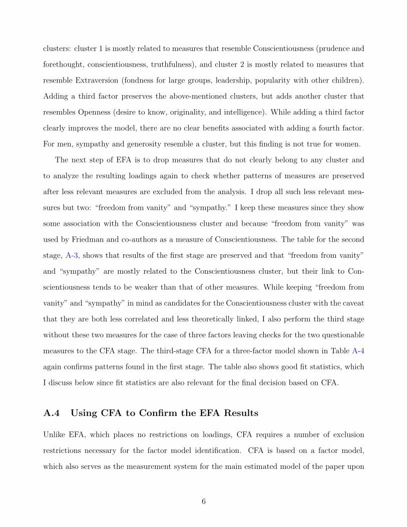
clusters: cluster 1 is mostly related to measures that resemble Conscientiousness (prudence and
forethought, conscientiousness, truthfulness), and cluster 2 is mostly related to measures that
resemble Extraversion (fondness for large groups, leadership, popularity with other children).
Adding a third factor preserves the above-mentioned clusters, but adds another cluster that
resembles Openness (desire to know, originality, and intelligence). While adding a third factor
clearly improves the model, there are no clear benefits associated with adding a fourth factor.
For men, sympathy and generosity resemble a cluster, but this finding is not true for women.
The next step of EFA is to drop measures that do not clearly belong to any cluster and
to analyze the resulting loadings again to check whether patterns of measures are preserved
after less relevant measures are excluded from the analysis. I drop all such less relevant mea-
sures but two: “freedom from vanity” and “sympathy.” I keep these measures since they show
some association with the Conscientiousness cluster and because “freedom from vanity” was
used by Friedman and co-authors as a measure of Conscientiousness. The table for the second
stage, A-3, shows that results of the first stage are preserved and that “freedom from vanity”
and “sympathy” are mostly related to the Conscientiousness cluster, but their link to Con-
scientiousness tends to be weaker than that of other measures. While keeping “freedom from
vanity” and “sympathy” in mind as candidates for the Conscientiousness cluster with the caveat
that they are both less correlated and less theoretically linked, I also perform the third stage
without these two measures for the case of three factors leaving checks for the two questionable
measures to the CFA stage. The third-stage CFA for a three-factor model shown in Table A-4
again confirms patterns found in the first stage. The table also shows good fit statistics, which
I discuss below since fit statistics are also relevant for the final decision based on CFA.
A.4 Using CFA to Confirm the EFA Results
Unlike EFA, which places no restrictions on loadings, CFA requires a number of exclusion
restrictions necessary for the factor model identification. CFA is based on a factor model,
which also serves as the measurement system for the main estimated model of the paper upon
6
being confirmed as acceptable.
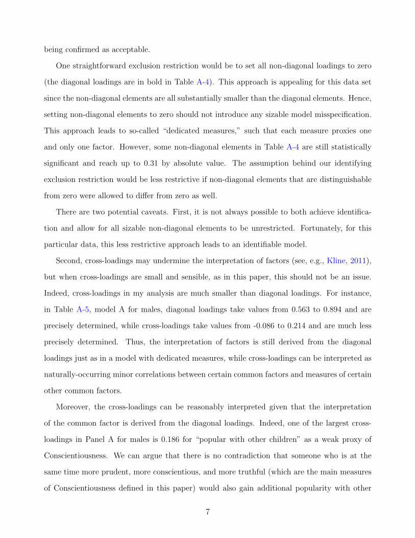
One straightforward exclusion restriction would be to set all non-diagonal loadings to zero
(the diagonal loadings are in bold in Table A-4). This approach is appealing for this data set
since the non-diagonal elements are all substantially smaller than the diagonal elements. Hence,
setting non-diagonal elements to zero should not introduce any sizable model misspecification.
This approach leads to so-called “dedicated measures,” such that each measure proxies one
and only one factor. However, some non-diagonal elements in Table A-4 are still statistically
significant and reach up to 0.31 by absolute value. The assumption behind our identifying
exclusion restriction would be less restrictive if non-diagonal elements that are distinguishable
from zero were allowed to differ from zero as well.
There are two potential caveats. First, it is not always possible to both achieve identifica-
tion and allow for all sizable non-diagonal elements to be unrestricted. Fortunately, for this
particular data, this less restrictive approach leads to an identifiable model.
Second, cross-loadings may undermine the interpretation of factors (see, e.g., Kline, 2011),
but when cross-loadings are small and sensible, as in this paper, this should not be an issue.
Indeed, cross-loadings in my analysis are much smaller than diagonal loadings. For instance,
in Table A-5, model A for males, diagonal loadings take values from 0.563 to 0.894 and are
precisely determined, while cross-loadings take values from -0.086 to 0.214 and are much less
precisely determined. Thus, the interpretation of factors is still derived from the diagonal
loadings just as in a model with dedicated measures, while cross-loadings can be interpreted as
naturally-occurring minor correlations between certain common factors and measures of certain
other common factors.
Moreover, the cross-loadings can be reasonably interpreted given that the interpretation
of the common factor is derived from the diagonal loadings. Indeed, one of the largest cross-
loadings in Panel A for males is 0.186 for “popular with other children” as a weak proxy of
Conscientiousness. We can argue that there is no contradiction that someone who is at the
same time more prudent, more conscientious, and more truthful (which are the main measures
of Conscientiousness defined in this paper) would also gain additional popularity with other
7

children. Similarly, there is no contradiction that desire to know also somewhat correlates with
Conscientiousness, as we expect conscientious people to look ahead and thus appreciate the
value of education (a small cross-loading of 0.065). Cross-loadings for Openness range from
-0.086 to 0.214 and include positive loadings for prudence and leadership and a negative one
for popularity. Interpretations of these small correlations are somewhat less straightforward,
but it is reasonable that a more original and intelligent person would also be better at planning
and leadership, while at the same time they may lose some popularity for being too different
from others (originality). Finally, extraversion has a small positive correlation with truthfulness
(loading 0.055) and a small negative correlation with the desire to know (-0.086). The negative
correlation is clear: extraverted people like socializing, which may limit spending time studying,
leading to smaller rating on the “desire to know,” since raters may associate the desire to
know with the amount of studying. Truthfulness might be a trait that is valued by people
one socializes with, possibly leading to a positive correlation with extraversion. The sign of
cross-loadings is preserved for females. Thus, cross-loadings that I allowed for milder exclusion
restrictions are small and do not contradict the interpretation of factors that is based on the
diagonal loadings.
I compare panel A in Table A-5 representing a model with cross-loadings based on stage
three of the EFA with three other panels: panel B represents a model with dedicated measures
only; panel C is a model with “freedom from vanity,” a questionable measure, allowed to affect
any factor as the least restrictive case to consider; and panel D, with “sympathy,” another
questionable measure, allowed to affect any factor. As I argue above, the fit measures are good
or fair for models B, C, and D, but model A shows the best fit and therefore I choose it as my
main model.
Goodness of Fit Goodness of fit statistics are described in many sources, such as Bollen and
Long (1993), Kline (2011), and Kolenikov (2009). Here I provide a short intuitive summary
and discuss the interpretation of results.
8
The Likelihood Ratio Test The likelihood ratio (LR) test, which is often referred to in
psychometric literature as “the Chi-square test,” compares two models: the constrained model,
which is the factor model that we test, and the unconstrained (unstructured, or saturated)
model, in which the model can exactly predict each observed covariance. Ideally, restrictions of
the factor model do not matter, so the test will not be rejected. In practice, this test is usually
rejected, leading some authors to doubt the reliability of the test (e.g., Bentler and Bonett, 1980;
Du and Tanaka, 1989) and ignore results of the test as uninformative or unreliable. Current
literature increasingly recognizes that the test should be taken seriously (see, e.g., Kline, 2011,
for a survey).
While I agree with the more recent claims that the test is generally reliable and informative
for the question being tested, I view frequent rejection of the test, even for otherwise clean
models, as a reasonable price for the major benefits of dimensionality reduction. We know that
statistics is an art of reasonable approximation, not exact fit, in line with which dimensionality
reduction techniques come at a cost of multiple model restrictions.6 The expectation that the
test will not be rejected is the expectation that a model with greatly reduced dimensionality
will still be exactly as informative as a fully saturated model, allowing for all possible correla-
tions between all possible measures. It would be over-optimistic to expect that none of these
restrictions will lead to at least some simplifications of reality.
My point is much in line with Steiger (2007) and Miles and Shevlin (2007). In particular,
Steiger notes that the chi-square test is not only about testing a hypothesis of a perfect fit,
which we know is always false, but also has the logical weakness inherent to the accept-support
tests: researchers who use tests with low power (say, those conducting studies with low sample
size) tend to accept the hypothesis and so support their model, while those using high power
tests tend to reject it and therefore have trouble defending their analysis. These properties
make the LR test not particularly useful, and so I do not use the LR test in this paper.
6A relevant quotation from statistician George Box is ”Essentially, all models are wrong, but some are useful”or another version, “...all models are wrong; the practical question is how wrong do they have to be to not beuseful” (Box, G. E. P., and Draper, N. R., (1987), Empirical Model Building and Response Surfaces, John Wiley& Sons, New York, NY).
9

The other fit statistics are called “approximate indexes.” Unlike the LR test, these are not
true statistical tests, but they are informative of the fit (Miles and Shevlin, 2007). Thresholds
(or “rules of thumb”) for these indices are recommended based on Monte-Carlo studies (Kline,
2011). I give a short overview of indices that I use below. For more detailed information and
formulas see, e.g., Bollen and Long (1993), Kline (2011), and Kolenikov (2009).
SRMR The Standardized Root-Mean-Square Residual (SRMR) is an absolute measure of
fit. It is a mean square root of a squared standardized difference between a true element of
the variance-covariance matrix and an element of the same matrix as predicted by the model.
Clearly, the smaller the SRMR, the better the model fit. The rule of thumb for a good fit is
SRMR≤0.08, which is satisfied for all models in Table A-5.
RMSEA Another index is the Root Mean Square Error of Approximation (RMSEA), which
is classified as a parsimony index. RMSEA is proportional to the square root of the likelihood
ratio from the LR test discussed above, so a lower number implies a better fit. RMSEA is
also inversely proportional to the square root of the number of model restrictions. If the
number of model restrictions is small, then RMSEA may become larger because of a decreased
denominator, which is a punishment for a non-parsimonious model. The rule of thumb is
RMSEA≤0.05, which is true for all models of types A and D in Table A-5.
CFI and TLI Finally, I use two comparative indices: the Comparative Fit Index (CFI)
and the Tucker-Lewis Index (TLI). These indices are relative because they are based on a
comparison of two likelihood ratios: (1) Target (constrained) model relative to unconstrained
(saturated) model; (2) Independence model (diagonal variance-covariance matrix) relative to
the target (constrained) model. Since measures are usually highly correlated, we expect our
target factor model to have much better fit than the independence model, which makes the
likelihood ratio (2) much larger than (1) and drives both indices close to 1. The rule of thumb
is that CFI and TLI > 0.9. In Table A-5 this is the case for all models of type A, C, and D.
To conclude, comparison of all approximate fit indices described above suggests that Model
10
A is preferable to model B, and that model A satisfies all recommended thresholds. Also, there
is no consistent evidence that models C and D are better than model A. Fit statistics for models
C and D tend to be worse or comparable to those for model A. Given doubts about theoretical
fit of “freedom from vanity” and “sympathy” to Conscientiousness, I chose model A as the most
reasonable model.
A.5 Using the 1940 Data to Augment the 1922 Factors
Analysis using the 1940 items that allow an inclusion of additional Big Five factors is docu-
mented in the Web Appendix to a companion paper by Savelyev and Tan (2019). Table A-6
summarizes results of the EFA and CFA of the companion paper. As mentioned in the main
text, I do not use the five-factor model as my preferred specification.
11

Fig
ure
A-1
:A
Phot
oco
py
ofO
ne
Ques
tion
from
the
Ori
ginal
1922
Ques
tion
nai
re:
Mea
suri
ng
Pru
den
cean
dF
oret
hou
ght
III.
RAT
ISU
GS
ON
PH
YSIC
AL,
MEN
TAL,
SQ
CIA
L,
AWD
M
QI?
.AL
TRAI
TS.
Dire
ctio
n!3:
(1
) In
ea
ch t
rait
or c
hara
cter
istic
na
med
bel
ow,
com
pare
thi
s ch
ild w
ith
the
aver
age c
hild
of t
he s
ame
age.
Th
en m
ake
a sm
all
cros
s so
mew
here
on
the
line
for
each
trai
t, to
sh
ow h
ow m
uch
of th
at t
rait
the
child
pos
sess
es.
Not
e th
at in
eac
h cas
e, on
e en
d of
the
line
repr
e-
sent
s on
e ex
trem
e fo
r th
e tra
it in
que
stio
n, a
nd th
e ot
her
end
of t
he li
ne t
he o
ther
ext
rem
e.
mid
dle
of t
he li
ne r
epre
sent
s an
ave
rage
am
ount
of
the
trait.
Th
e
stat
ed in
fine
prin
t ab
ove
the
line.
Th
e m
eani
ngs
of o
ther
poi
nts
arc
Befo
re m
akin
g th
e cr
oss,
read
ver
y ca
refu
lly e
very
thin
g th
at i
s pr
inte
d in
sm
all t
ype
abov
e th
e lin
e.
(2)
Try
to m
ake
real
dis
tinct
ions
. ex
cept
iona
l in
som
e.
Do
not
rate
a c
hild
hig
h on
all
traits
sim
ply
beca
use h
e is
C
hild
ren
are
ofte
n ve
ry h
igh
in s
ome
traits
and
ver
y lo
w i
n ot
hers
. (3
) Lo
cate
you
r cr
oss
any
plac
e on
the
line
whe
re y
ou t
hink
it
belo
ngs.
to
loca
te it
at a
ny o
f the
littl
e ve
rtica
l m
arks
. It
is n
ot n
eces
sary
(4)
Do
not
stud
y to
o lo
ng o
ver
any
one
trait.
go
on
to th
e ne
xt.
Plea
se o
mit
none
. G
ive
for
each
the
best
judg
men
t yo
u ca
n, a
nd
The
ratin
gs w
ill be
hel
d ab
solu
tely
con
fiden
tial.
(5)
Belo
w e
ach
line,
und
erlin
e th
e w
ord
that
tel
ls h
ow c
erta
in y
ou f
eel a
bout
you
r ju
dgm
ent.
Exam
pla:
In
Exa
mpl
e 1,
the
cros
s sh
ows
how
one
chi
ld ia
s ra
ted
for
beau
ty,
and
the
line
unde
rnea
th t
he w
ords
“ve
ry c
erta
in”
show
s th
at t
he o
ne w
ho m
ade
the
ratin
g fe
lt “v
ery
certa
in”
of h
is ju
dgm
ent.
In E
xam
ple
2 th
e cr
oss
show
s ho
w t
he s
ame
child
was
rat
ed f
or
obst
inac
y,
and
the
line
unde
r “fa
irly
certa
in”
show
s th
at t
he o
ne w
ho m
ade
the
ratin
g fe
lt “fa
irly
certa
in”
of h
is j
udgm
ent.
Do
not
rate
thi
s ch
ild o
n th
e “e
xam
ples
.”
Exam
ple
1. B
eaut
y.
Extra
ordi
nary
D
ecid
ed1
Rnt
her
beau
ty an
d cha
rm
benu
tifu Y
be
autif
ul
Rnt
hcr
hom
ely
Extre
mel
y ug
ly
and
repu
lsiv
e t
I ,
I I
I I
I ,
X--i-
---l
WSS
JOW
Ju
dmen
t on
th
a ab
ove
trolt
very
co
rtaln
, lft
lrlp
corta
ln,
r&tb
er n
ncer
tab,
ve
rg u
ncer
tdn?
Exam
ple
2. Q
bstin
acy.
Ex
traor
dina
rily
Dec
idrd
ly
obst
inat
e an
d R
athe
r D
ecid
edly
obst
inat
e and
stub
born
st
ubbo
rn
obst
inat
e “i,
v:~~
ee
Less
thou
le
es th
an
Extre
me
lack
av
erag
e av
erag
e t--
----x
7--u
-i of
obr
tiarc
, t
I 1
I I
I -i
War
you
r ju
dgm
ant
on t
ba a
bove
trul
t ve
ry
crrta
ln,
Iolrl
y cs
rteln
, ra
ther
unc
erta
in,
vorg
unc
ar&&
T
w
Begi
n w
ith
Trai
t 1,
Hea
lth
Trai
t 1,
N
ealth
. Ex
traor
dina
rily
Goo
d D
ecid
edly
R
athe
r R
othe
r he
alth
. Al
mos
t nev
er
supe
rior
supe
rior
wea
k1
heal
th
heal
th
3ov,
e:;:
r D
z%~1
y Ex
trem
ely
wea
kly a
nd
sick
. Vi
goro
us.
or s
ick y
or
sic
k T
sick
ly.
Extre
me
y t
t I
I la
ck o
f vig
or.
I I
I I
I 4
Wna
your
Judc
mon
ton th
e abo
vo tra
it VW
cef
Mn,
lalrl
9 cer
tsln
, rathe
r nn
certa
ln, vary
un
csrts
in~
(Und
grbe
)
Trai
t 2.
Am
ount
of
phy
sica
l en
ergy
. Ex
traor
dina
ry a
mou
nt
of p
hysi
cal e
nerp
. “p
ep” a
nd an
imot
lon.
D
ynam
ic a
nd tir
eles
s.
Dec
ided
ly
mor
e th
an
aver
age
Rat
her
mor
e th
an
aven
ge
Extre
me
phyr
ial
iner
tia a
nd la
ck o
f “p
ep.”
Slqg
ish
and
CflJ
ily
fatw
ed.
t I
I I
I I
I I
I I
1 I
Waa
you
r Ju
dgm
ent o
n th
e @
bore
traf
t v0
rY c
erta
in,
!akl
Y ce
rtaha
. rat
her
unce
rtafn
, ve
ry u
ncer
tain
? (U
ndor
Une
)
Trai
t 3.
Pr
uden
ce a
nd fo
reth
ough
t. Ex
xtno
rdin
nry
pmde
nce
Alw
ays
look
s ah
ead
Nev
er s
acrif
ices
futu
re
Dec
ided
ly
Rat
her
Rat
her
Extre
me
lack
of
good
for p
rese
nt
mor
e pr
uden
t m
ore
prud
ent
plea
sure
. th
an a
vera
ge
than
ave
rage
%
‘:FgF
ho
upt
;;ys”
D
ecid
edly
pr
uden
ce.
Nev
er lo
oks
T ha
UPc
Y;yP
o-
P ah
ead.
Liv
es w
holb
in
the
pres
ent.
t I
I I
, 1
, t-
Was
you
r Ju
dgm
ent o
n th
e rb
ovcl
tra
it VO
?Y c
art%
& fa
lrlp
certa
in.
rotb
or u
ncer
tain
, ve
ry u
ncer
tain
? (U
nder
lIne)
-3-
Source:
Ter
man
and
Sea
rs(2
002)
.R
esp
ond
ents
wer
eas
ked
top
ut
am
ark
anyw
her
eon
this
lin
e.
12
Fig
ure
A-2
:Scr
eeP
lots
(a)
Mal
es(b
)F
emal
es
0
0.51
1.52
2.53
3.54
4.55
02
46
810
1214
16
0
0.51
1.52
2.53
3.54
4.55
02
46
810
12
14
16
Notes:
Scr
eep
lots
are
show
nfo
r15
item
sp
oten
tial
lyre
late
dto
the
Big
Fiv
etr
aits
.C
alcu
lati
ons
are
bas
edon
the
Ter
man
dat
a.
13

Table A-1: Estimates of the Number of Factors Based on Various Methods
Procedure Males Females
Scree(a)
2 3
Guttman-Kaiser(b)
4 4
Horn(c)
4 3
Minap(d)
3 2
Onatski(e)
3-7 factors 3 -
2-7 factors 2 -
1-7 factors 2 -
Notes:(a)Scree test is by Cattell (1966). The corresponding scree plots are documented in Figure A-2.(b)See Gorsuch (1983); Guttman (1954); Kaiser (1960, 1961) for a discussion of the Guttman-Keiser rule. Themethod is known to exclude factors that clearly have little explanatory power, but it often overestimates thenumber of informative factors (Zwick and Velicer, 1986).(c)Horn’s (1965) parallel analysis procedure.(d)See Velicer (1976) for the Minap description.(e)We apply Onatski’s (2009) procedure at the 5% level of significance for a minimum of three, two, and one
factors and for a maximum of seven factors. Onatski (2009) warns that the asymptotic approximation may
be poor in a case where sample size is small and the number of measures is low. “-” denotes that Onatski’s
algorithm does not converge to any number in the given range.
14

Table A-2: First Stage of the EFA
Males 1 2 1 2 3 1 2 3 4
Prudence and forethought 0.697* -0.086* 0.623* 0.160* -0.119* 0.722* 0.112* 0.038 -0.143*
Conscientiousness 0.862* -0.054* 0.827* 0.076* -0.066* 0.775* 0.060* -0.015 0.112*
Truthfulness 0.771* 0.012 0.768* 0.031 0.008 0.673* 0.031 0.015 0.170*
Desire to know 0.371* 0.143* 0.076* 0.721* -0.041 0.075* 0.719* -0.070* 0.034
Originality 0.295* 0.233* 0.011 0.679* 0.069* 0.037 0.673* 0.064 -0.019
Intelligence 0.300* 0.241* 0.022 0.680* 0.076* 0.009 0.687* 0.027 0.052
Fondness for large groups -0.163* 0.730* -0.147* 0.026 0.717* -0.261* 0.060 0.566* 0.227*
Leadership 0.039 0.579* -0.032 0.200* 0.537* 0.055 0.170* 0.653* -0.156*
Popularity w other children 0.061* 0.699* 0.113* -0.062* 0.744* 0.098* -0.094* 0.813* 0.031
Optimism 0.064 0.596* 0.006 0.190* 0.538* -0.137* 0.229* 0.375* 0.277*
Permanency of moods 0.330* 0.228* 0.314* 0.065 0.213* 0.317* 0.049 0.256* 0.004
Sensitiveness 0.270* 0.150* 0.251* 0.066 0.132* 0.118* 0.095* 0.013 0.262*
Freedom from vanity 0.457* 0.050 0.585* -0.245* 0.125* 0.468* -0.244* 0.108* 0.217*
Sympathy 0.443* 0.239* 0.453* 0.021 0.231* 0.142* 0.087* -0.049 0.626*
Generosity 0.404* 0.381* 0.440* -0.021 0.390* 0.134* 0.035 0.135* 0.606*
Sample size
Females
Prudence and forethought 0.587* 0.015 0.562* 0.068 -0.007 0.587* 0.057 0.026 -0.039
Conscientiousness 0.872* -0.053* 0.845* 0.041 -0.048* 0.868* 0.021 -0.017 0.007
Truthfulness 0.772* -0.003 0.734* 0.103* -0.048 0.745* 0.091* -0.016 -0.005
Desire to know 0.245* 0.332* 0.043 0.680* -0.054 0.046 0.678* -0.048 0.002
Originality 0.214* 0.414* 0.045 0.597* 0.075 0.026 0.592* 0.071 0.051
Intelligence 0.258* 0.372* 0.062 0.683* -0.005 0.049 0.686* -0.008 0.027
Fondness for large groups -0.179* 0.639* -0.133* -0.020 0.712* -0.130* -0.038 0.720* 0.004
Leadership -0.082* 0.665* -0.148* 0.347* 0.474* -0.130* 0.332* 0.483* -0.019
Popularity w other children 0.129* 0.606* 0.190* -0.046 0.720* 0.168* -0.054 0.718* 0.035
Optimism 0.067 0.572* 0.043 0.215* 0.460* 0.052 0.205* 0.479* -0.023
Permanency of moods 0.288* 0.200* 0.300* 0.021 0.200* 0.352* 0.013 0.233* -0.056
Sensitiveness 0.291* 0.090 0.309* -0.032 0.136* 0.199* -0.024 0.089 0.212*
Freedom from vanity 0.572* -0.104* 0.629* -0.168* 0.015 0.583* -0.159* 0.018 0.058
Sympathy 0.474* 0.197* 0.485* 0.028 0.204* -0.006 0.005 -0.004 1.191*
Generosity 0.517* 0.229* 0.528* 0.042 0.223* 0.373* 0.053 0.167* 0.291*
Sample size 536 536 536
2 factors 3 factors 4 factors
695 695 695
Notes: An asterisk denotes a 5% level statistical significance.
15

Table A-3: Second Stage of the EFA
Male 1 2 1 2 3 1 2 3 4
Prudence and forethought 0.690* -0.044 0.627* 0.130* -0.056 0.634* 0.085* -0.023 -0.265*
Conscientiousness 0.858* -0.031 0.837* 0.054* -0.033 0.822* 0.060* -0.016 -0.033
Truthfulness 0.774* 0.004 0.783* 0.010 0.017 0.781* 0.042 0.004 0.110*
Desire to know 0.387* 0.137* 0.082* 0.710* -0.040 0.069* 0.740* -0.061* 0.054
Originality 0.309* 0.223* 0.005 0.690* 0.051 -0.001 0.668* 0.069* -0.101*
Intelligence 0.319* 0.225* 0.024 0.690* 0.049 0.016 0.700* 0.044 0.045
Fondness for large groups -0.133* 0.688* -0.149* 0.073 0.627* -0.134* 0.079* 0.639* 0.223*
Leadership 0.054 0.643* -0.042 0.225* 0.567* -0.030 0.139* 0.657* -0.254*
Popularity w other children 0.065* 0.737* 0.079* -0.055* 0.862* 0.118* -0.077* 0.800* 0.022
Freedom from vanity 0.435* 0.049 0.549* -0.232* 0.153* 0.560* -0.219* 0.128* 0.054
Sympathy 0.436* 0.181* 0.422* 0.055 0.162* 0.430* 0.103* 0.135* 0.259*
Sample size
Female
Prudence and forethought 0.577* 0.055 0.560* 0.063 0.028 0.461* 0.102 0.029 0.085
Conscientiousness 0.893* -0.021 0.890* 0.013 0.000 1.029* -0.025 0.002 -0.028*
Truthfulness 0.770* 0.023 0.738* 0.090* -0.02 0.514* 0.164* -0.016 0.219*
Desire to know 0.235* 0.372* 0.041 0.676* -0.067* 0.059 0.672* -0.063 -0.062
Originality 0.199* 0.498* 0.041 0.601* 0.094 -0.003 0.617* 0.093* 0.014
Intelligence 0.246* 0.417* 0.053 0.690* -0.013 -0.017 0.717* -0.014 0.059
Fondness for large groups -0.154* 0.548* -0.119* -0.025 0.692* -0.019 -0.064 0.694* -0.121*
Leadership -0.091* 0.750* -0.134* 0.336* 0.516* -0.018 0.299* 0.522* -0.174*
Popularity w other children 0.137* 0.532* 0.185* -0.046 0.729* 0.040 -0.013 0.741* 0.173*
Freedom from vanity 0.552* -0.129* 0.585* -0.141* 0.010 0.044 0.000 0.005 0.719*
Sympathy 0.430* 0.179* 0.415* 0.073 0.181* 0.157* 0.155* 0.178* 0.302*
Sample size 536 536 536
2 factors 3 factors 4 factors
695 695 695
Notes: An asterisk denotes a 5% level statistical significance.
16

Table
A-4
:T
hir
dSta
geof
the
EFA
,a
Thre
e-F
acto
rC
ase
Conscientiousness
Standard Error
Openness
Standard Error
Extraversion
Standard Error
Conscientiousness
Standard Error
Openness
Standard Error
Extraversion
Standard Error
Conscientiousness
Pruden
ce0.628
(0.035)
0.108
(0.040)
‐0.037
(0.032)
0.541
(0.041)
0.070
(0.051)
0.030
(0.046)
Conscientiousness
0.904
(0.027)
‐0.016
(0.018)
‐0.002
(0.015)
0.977
(0.031)
‐0.028
(0.012)
0.007
(0.013)
Truthfulness
0.740
(0.032)
0.003
(0.031)
0.045
(0.026)
0.682
(0.038)
0.111
(0.042)
‐0.016
(0.033)
Open
ness
Desire to know
0.072
(0.032)
0.707
(0.036)
‐0.055
(0.025)
0.036
(0.033)
0.666
(0.045)
‐0.055
(0.034)
Originality
‐0.019
(0.028)
0.711
(0.036)
0.033
(0.028)
0.024
(0.036)
0.604
(0.052)
0.099
(0.049)
Intelligence
‐0.002
(0.028)
0.713
(0.035)
0.032
(0.027)
0.030
(0.030)
0.713
(0.044)
‐0.019
(0.032)
Extraversion
Fondness for large groups
‐0.133
(0.032)
0.040
(0.039)
0.640
(0.036)
‐0.079
(0.033)
‐0.061
(0.035)
0.716
(0.043)
Leadership
‐0.017
(0.033)
0.193
(0.042)
0.582
(0.036)
‐0.105
(0.033)
0.308
(0.056)
0.534
(0.051)
Popular with other children
0.080
(0.022)
‐0.066
(0.016)
0.838
(0.035)
0.172
(0.033)
‐0.023
(0.038)
0.690
(0.046)
Root mean square error of approximation (RMSEA)
90 Percent C.I.
Probability RMSEA <= .05
Comparative fit index (CFI)
Tucker‐Lew
is index (TLI)
Standardized
root‐mean‐square‐residual (SRMR)
Sample size
Males
Females
0.049
0.047
(0.029, 0.070)
(0.022, 0.072)
0.485
0.535
0.016
0.017
695
536
0.989
0.968
0.989
0.967
Notes:
Fac
tor
load
ings
are
bas
edon
obli
qu
equ
arti
min
rota
tion
.F
acto
rlo
adin
gsre
lati
ng
fact
ors
toth
em
ain
corr
esp
ond
ing
mea
sure
sare
inb
old
.
Cal
cula
tion
sar
eb
ased
onth
eT
erm
and
ata.
17

Table
A-5
:M
LC
FA
Res
ult
sfo
rth
eC
OE
-192
2M
odel
Factor Loading
Standard Error
Factor Loading
Standard Error
Factor Loading
Standard Error
Factor Loading
Standard Error
Factor Loading
Standard Error
Factor Loading
Standard Error
Factor Loading
Standard Error
Factor Loading
Standard Error
Conscientiousness (C)
Prudenc e
0.623
(0.043)
0.678
(0.037)
0.638
(0.042)
0.616
(0.042)
0.554
(0.048)
0.588(0.043)
0.565
(0.048)
0.556
(0.048)
Conscientiousness
0.894
(0.036)
0.884
(0.035)
0.851
(0.034)
0.896
(0.035)
0.931
(0.041)
0.925(0.040)
0.894
(0.038)
0.922
(0.039)
Truthfulness
0.748
(0.037)
0.756
(0.036)
0.782
(0.035)
0.750
(0.036)
0.746
(0.042)
0.750(0.041)
0.773
(0.039)
0.753
(0.040)
Desire to know
0.065
(0.042)
‐‐
0.045
(0.044)
0.068
(0.042)
0.003
(0.053)
‐‐
‐0.016
(0.056)
‐0.001
(0.053)
Popular with other children
0.186
(0.046)
‐‐
0.241
(0.051)
0.183
(0.045)
0.295
(0.054)
‐‐
0.341
(0.060)
0.314
(0.057)
Freedom from vanity
‐‐
‐‐
0.588
(0.049)
‐‐
‐‐
‐‐
0.596
(0.056)
‐‐
Sympathy
‐‐
‐‐
‐‐
0.434
(0.044)
‐‐
‐‐
‐‐
0.420
(0.052)
Open
ness (O)
Desire to
know
0.715
(0.048)
0.738
(0.039)
0.731
(0.049)
0.715
(0.048)
0.677
(0.063)
0.657(0.046)
0.696
(0.066)
0.681
(0.064)
Originality
0.710
(0.039)
0.693
(0.039)
0.703
(0.039)
0.710
(0.039)
0.658
(0.047)
0.630(0.047)
0.656
(0.046)
0.659
(0.047)
Intelligence
0.720
(0.038)
0.721
(0.039)
0.713
(0.038)
0.720
(0.038)
0.708
(0.046)
0.734(0.046)
0.698
(0.045)
0.708
(0.045)
Pruden
ce0.107
(0.042)
‐‐
0.093
(0.042)
0.109
(0.042)
0.075
(0.050)
‐‐
0.061
(0.050)
0.070
(0.049)
Leadership
0.214
(0.048)
‐‐
0.211
(0.048)
0.213
(0.047)
0.329
(0.051)
‐‐
0.331
(0.051)
0.325
(0.051)
Popular with other children
‐0.086
(0.061)
‐‐
‐0.152
(0.069)
‐0.082
(0.060)
‐0.001
(0.069)
‐‐
‐0.046
(0.075)
‐0.021
(0.073)
Freedom from vanity
‐‐
‐‐
‐0.277
(0.052)
‐‐
‐‐
‐‐
‐0.168
(0.061)
‐‐
Sympathy
‐‐
‐‐
‐‐
0.039
(0.047)
‐‐
‐‐
‐‐
0.094
(0.059)
Extraversion (E)
Fondness fo
r large
groups
0.628
(0.042)
0.613
(0.040)
0.604
(0.043)
0.638
(0.042)
0.691
(0.052)
0.625(0.049)
0.685
(0.052)
0.679
(0.052)
Lead
ership
0.563
(0.042)
0.651
(0.042)
0.540
(0.043)
0.561
(0.041)
0.507
(0.048)
0.668(0.053)
0.508
(0.048)
0.497
(0.048)
Popular w
ith other child
ren
0.840
(0.050)
0.811
(0.043)
0.901
(0.055)
0.832
(0.049)
0.693
(0.060)
0.684(0.052)
0.716
(0.065)
0.720
(0.063)
Truthfulness
0.055
(0.033)
‐‐
0.047
(0.033)
0.056
(0.033)
0.015
(0.038)
‐‐
0.005
(0.038)
0.014
(0.038)
Desire to know
‐0.083
(0.039)
‐‐
‐0.082
(0.039)
‐0.083
(0.039)
‐0.083
(0.055)
‐‐
‐0.094
(0.056)
‐0.088
(0.055)
Freedom from vanity
‐‐
‐‐
0.200
(0.042)
‐‐
‐‐
‐‐
0.012
(0.054)
‐‐
Sympathy
‐‐
‐‐
‐‐
0.183
(0.041)
‐‐
‐‐
‐‐
0.172
(0.052)
Root mean sq. err. of approx. (RMSEA)
90 Percent C.I.
Probability RMSEA <= .05
Comparative fit index (CFI)
Tucker‐Lew
is index (TLI)
Stand. root‐mean‐sq.‐resid. (SRMR)
Sample size
Males
Females
model A
model B
model C
model D
model A
model B
model C
model D
0.989
0.960
0.973
0.983
0.983
0.930
0.974
0.982
0.948
0.965
0.042
0.067
0.059
0.047
0.050
0.085
0.056
0.046
0.976
0.941
0.947
0.967
0.963
0.895
0.026
0.024
695
695
695
695
536
536
536
536
0.021
0.046
0.026
0.023
0.024
0.056
(0.070, 0.101)
(0.040, 0.073)
(0.028, 0.064)
0.736
0.020
0.130
0.611
0.462
0.000
0.246
0.628
(0.024, 0.060)
(0.053, 0.081)
(0.045, 0.074)
(0.032, 0.062)
(0.030, 0.071)
Notes:
Fac
tor
load
ings
are
bas
edon
the
con
firm
ator
yfa
ctor
anal
ysi
s.F
acto
rlo
adin
gsre
lati
ng
fact
ors
toth
eco
rres
pon
din
gp
ossi
ble
ded
icate
dm
easu
res
are
inb
old
.C
alcu
lati
ons
are
bas
edon
the
Ter
man
dat
a.
18
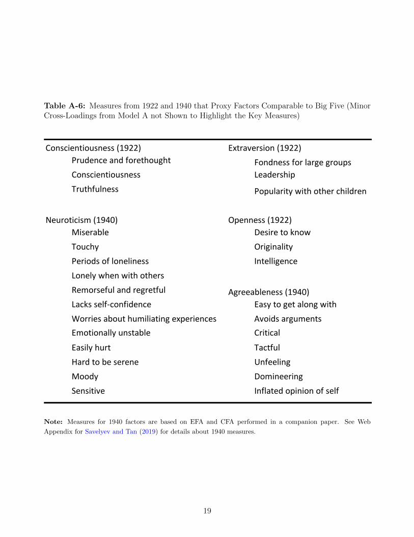
Table A-6: Measures from 1922 and 1940 that Proxy Factors Comparable to Big Five (MinorCross-Loadings from Model A not Shown to Highlight the Key Measures)
Conscientiousness (1922) Extraversion (1922)
Prudence and forethought Fondness for large groups
Conscientiousness Leadership
Truthfulness Popularity with other children
Neuroticism (1940) Openness (1922)
Miserable Desire to know
Touchy Originality
Periods of loneliness Intelligence
Lonely when with others
Remorseful and regretful Agreeableness (1940)
Lacks self-confidence Easy to get along with
Worries about humiliating experiences Avoids arguments
Emotionally unstable Critical
Easily hurt Tactful
Hard to be serene Unfeeling
Moody Domineering
Sensitive Inflated opinion of self
Note: Measures for 1940 factors are based on EFA and CFA performed in a companion paper. See Web
Appendix for Savelyev and Tan (2019) for details about 1940 measures.
19

B Supplementary Figures and Tables
The section below is composed of figures and tables that are mentioned in various parts of the
main paper as supplementary. Each paragraph below shortly describes one or several tables or
figures.
Evolution of School Enrollment Figure B-1 shows the evolution of school enrollment,
which sharply decreases with age. By age 30, only about 5% of the Terman population are in
school. As discussed in the main paper, this result is one argument for the low likelihood of a
reverse causal interpretation of results in a model conditional on survival to age 30.
Comparison of Models with Varying Starting Age Table B-1 shows that results of the
model are robust to starting age from about age 12 (year 1922) to age 30. One reason for
similar coefficients is low mortality before age 30.
MPH Model of Mortality and Logit Models if Education Choice for Females Table
B-2 represents results of the Cox model for females and supplements the corresponding table
for males (see Table 4 of the main paper). Unlike for males, neither single nor joint tests can
be rejected.
The Measurement System The measurement system is an integral part of the system
of equations jointly estimated in this paper, which allows the identification of the effect of
latent factors on education and the hazard of death. Table B-3 shows that the main loadings,
measures for which are shown in bold, are all statistically significant at the 1% level and tend
to be of substantial size, around 0.5–0.9 or higher.7 In contrast, the cross-loadings measures
(not in bold) are substantially smaller than the main loadings and tend to be less precisely
determined. This observation is important since we use measures associated with the main
loadings to interpret the factor, while cross-loadings account for small correlations that we
7The first loading is not 1 since I used a standard alternative normalization: setting variance of all latentfactors to 1.
20

allow in order to make plausible exclusion restrictions, as discussed in detail in Web Appendix
A.
Checking Robustness of Estimates with Respect to Exclusion of Certain Groups
from the Sample Table B-4 shows the Cox model results for males for the full sample and
various sub-samples. Sub-samples are the following: (1) violent deaths omitted; (2) suicides
omitted; (3) auto crashes omitted; (4) alcohol-related deaths omitted; (5) all unknown causes
of death omitted. We see that results are robust to excluding specific groups outlined above
(there is some variation of estimates across cases, but results are qualitatively the same and
numerically similar).
Robustness of the Main Model Based on 1922 Personality Measures to the Inclusion
of Agreeableness and Neuroticism Factors Based on Measures from 1940 Table B-5
compares a three-factor with a five-factor model. From the comparison we see that regression
coefficients for Agreeableness and Neuroticism are small and statistically insignificant, both
individually and jointly (the p-value for the Wald test is 0.960). We can also see that the
omission of these two factors leads to only small changes in other regression coefficients. The
omission of the two factors leads to a strong reduction in degrees of freedom and improvement
in numerical stability of the model.
Robustness of the Main Full Likelihood Model to a Two-Step Estimation As dis-
cussed in the main paper, one common concern about using a full maximum likelihood model
in research involving latent skills is that in the case of model misspecification, skills might be
primarily driven by outcomes rather than the measurement system. Table B-6 shows that this
concern is not pertinent to results of this paper. For Model 2 of the table, I follow Heckman
et al. (2018) and estimate only the measurement system in the first step and then estimate
the maximum likelihood model while fixing loadings of the measurement system to the values
estimated in the first step. The estimates of Model 2 are almost identical to those of Model 1
based on full maximum likelihood.
21

Fig
ure
B-1
:E
volu
tion
ofSch
ool
Enro
llm
ent∗
020406080100
% enrolled at school
1516
1718
1920
2122
2324
2526
2728
2930
3132
3334
3536
3738
3940
Age
Notes:
(*)A
tten
din
gh
igh
sch
ool
,u
nd
ergr
adu
ate,
orgr
adu
ate
sch
ool
.C
alcu
lati
ons
are
bas
edon
the
Ter
man
dat
a.
22

Table
B-1
:C
ompar
ison
ofM
odel
sw
ith
Var
yin
gSta
rtin
gA
ge,
Mal
es
Edu
cati
on
Hig
h s
cho
ol
0.7
31
***
–0
.71
2**
*–
0.7
37
***
–0
.75
2**
*–
0.7
74
***
–
d
egre
e(0.183)
–(0.185)
–(0.186)
–(0.187)
–(0.188)
–
Som
e co
llege
0
.45
2**
*–
0.3
94
***
–0
.38
9**
*–
0.3
87
***
–0
.39
4**
*–
ed
uca
tio
n(0.141)
–(0.143)
–(0.144)
–(0.144)
–(0.144)
–
Bac
hel
or'
s d
egre
e
o
r ab
ove
Skill
s Co
nsc
ien
tio
usn
ess
-0.1
38
*0
.19
9-0
.14
5*
0.2
04
-0.1
41
*0
.20
5-0
.13
0*
0.2
18
*-0
.12
9*
0.2
10
*
(0.073)
(0.126)
(0.075)
(0.129)
(0.075)
(0.128)
(0.074)
(0.128)
(0.073)
(0.127)
Extr
aver
sio
n-0
.12
2*
-0.1
69
-0.1
23
*-0
.16
6-0
.12
3*
-0.1
67
-0.1
28
*-0
.17
2-0
.13
8*
-0.1
63
(0.070)
(0.123)
(0.071)
(0.124)
(0.071)
(0.124)
(0.071)
(0.125)
(0.071)
(0.125)
Op
enn
ess
0.1
14
0.1
67
0.0
96
0.1
84
0.0
90
0.1
82
0.0
93
0.1
75
0.0
93
0.1
78
(0.081)
(0.145)
(0.082)
(0.150)
(0.082)
(0.148)
(0.083)
(0.148)
(0.082)
(0.147)
IQ-0
.05
00
.29
8**
*-0
.03
40
.29
5**
*-0
.02
80
.29
8**
*-0
.02
70
.29
7**
*-0
.02
50
.29
9**
*
(0.062)
(0.103)
(0.062)
(0.103)
(0.062)
(0.103)
(0.063)
(0.103)
(0.062)
(0.105)
Ob
serv
atio
ns
71
17
06
70
27
00
69
5
o
mit
ted
o
mit
ted
Star
tin
g A
ge 3
0
Mo
rtal
ity
Edu
cati
on
MP
HO
rder
ed
(1)
(2)
Star
tin
g A
ge 2
7
Mo
rtal
ity
Edu
cati
on
MP
HO
rder
ed
o
mit
ted
o
mit
ted
o
mit
ted
(1)
(2)
(1)
(2)
(1)
(2)
(1)
(2)
Edu
cati
on
MP
HO
rder
ed
MP
HO
rder
ed
MP
HO
rder
ed
Age
at
Star
t (Y
ear
19
22
)St
arti
ng
Age
23
Star
tin
g A
ge 2
5
Mo
rtal
ity
Edu
cati
on
Mo
rtal
ity
Edu
cati
on
Mo
rtal
ity
Notes:
Mod
elco
effici
ents
are
pre
sente
dw
ith
stan
dar
der
rors
show
nin
par
enth
eses
.F
orth
ep
urp
ose
ofnu
mer
ical
ly-s
tab
lero
bu
stn
ess
chec
k,
Ico
nd
itio
n
all
mod
els
onb
ackgr
oun
dco
ntr
ols
bu
tn
oton
unob
serv
edh
eter
ogen
eity
.A
ster
isks
den
ote
stat
isti
cal
sign
ifica
nce
:**
*1%
leve
l;**
5%le
vel;
*10%
level
.
23

Table
B-2
:M
PH
Model
ofM
orta
lity
and
Log
itM
odel
sof
Educa
tion
Choi
ce,
Fem
ales
PH
-te
st
Ou
tco
me
Su
b-M
od
el T
yp
e
(9)
Hig
h s
cho
ol
-0.0
42
–-0
.04
2–
-0.0
2–
-0.0
1-0
.00
30
.58
9
d
eg
ree
(0.271)
–(0.268)
–(0.269)
–(0.270)
(0.240)
So
me
co
lle
ge
-0
.15
6–
-0.1
4–
-0.1
11
–-0
.10
3-0
.03
90
.62
9
e
du
cati
on
(0.209)
–(0.200)
–(0.197)
–(0.195)
(0.184)
Ba
che
lor'
s d
eg
ree
o
r a
bo
ve
Co
nsc
ien
tio
usn
ess
0.1
53
-0.2
26
-0.1
39
0.2
08
––
––
-0
.69
3
(0.109)
(0.162)
(0.102)
(0.148)
––
––
-
Extr
ave
rsio
n0
.05
7-0
.18
80
.00
3-0
.18
9–
––
–-
0.8
76
(0.113)
(0.153)
(0.103)
(0.145)
––
––
-
Op
en
ne
ss-0
.11
9-0
.05
60
.12
40
.06
7–
––
–-
0.1
75
(0.134)
(0.185)
(0.125)
(0.175)
––
––
-
IQ-0
.01
80
.10
3-0
.09
80
.11
2-0
.08
00
.16
3–
–-
0.7
32
(0.101)
(0.124)
(0.094)
(0.115)
(0.087)
(0.114)
––
-
Join
t te
st p
-va
lue
s0
.85
97
Un
ob
s. H
ete
rog
en
eit
y (τ
)
Ba
ckg
rou
nd
co
ntr
ols
(X
)
Mo
rta
lity
MP
H
Mo
rta
lity
MP
H
Mo
de
l 1
Mo
de
l 2
Mo
de
l 3
Mo
de
l 4
Ord
ere
d lo
git
Ord
ere
d lo
git
Ord
ere
d lo
git
Mo
rta
lity
MP
H
Ed
uca
tio
nM
ort
ality
Ed
uca
tio
n
MP
H
Mo
rta
lity
Ed
uca
tio
n
MP
H
(5)
(6)
(7)
om
itte
do
mit
ted
om
itte
do
mit
ted
(1)
(2)
(3)
(4)
Ye
sY
es
Ye
sY
es
No
0.8
23
80
.68
81
0.8
52
20
.86
55
Ye
sN
oN
oN
o
Mo
de
l 5
(8)
om
itte
d
0.9
77
0
No
Notes:
Mod
elco
effici
ents
are
pre
sente
dw
ith
stan
dar
der
rors
show
nin
par
enth
eses
.T
he
tab
lesh
ows
the
sam
em
od
elas
Tab
le4
ofth
em
ain
pap
er,
bu
t
for
fem
ales
.R
esu
lts
are
bas
edon
the
Ter
man
dat
a.
24
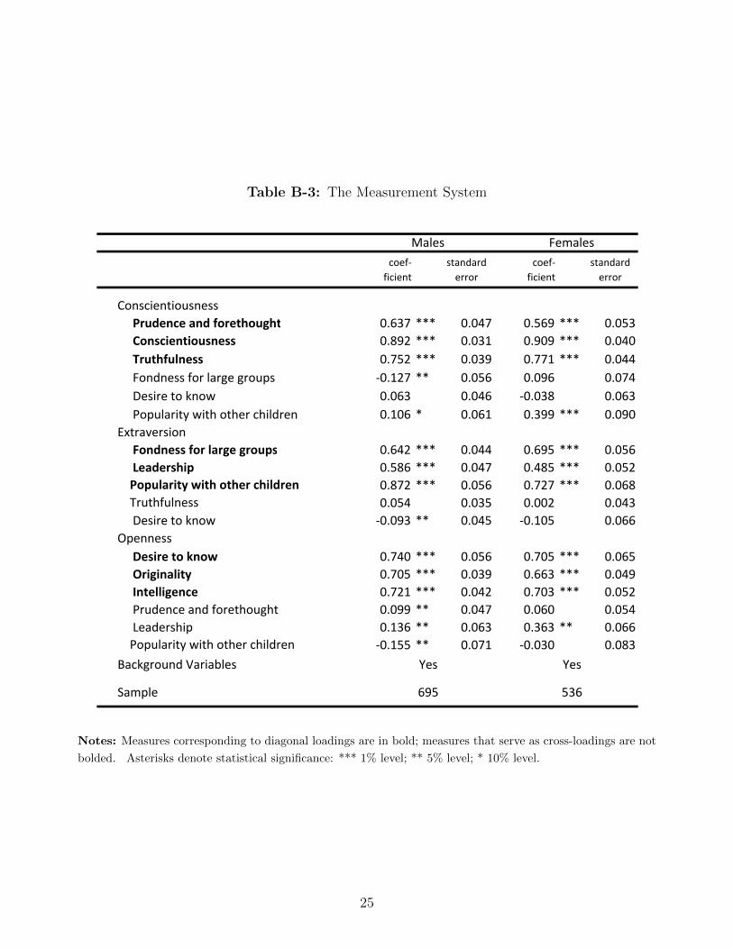
Table B-3: The Measurement System
coef‐
ficient
standard
error
coef‐
ficient
standard
error
Conscientiousness
Prudence and forethought 0.637 *** 0.047 0.569 *** 0.053
Conscientiousness 0.892 *** 0.031 0.909 *** 0.040
Truthfulness 0.752 *** 0.039 0.771 *** 0.044
Fondness for large groups ‐0.127 ** 0.056 0.096 0.074
Desire to know 0.063 0.046 ‐0.038 0.063
Popularity with other children 0.106 * 0.061 0.399 *** 0.090
Extraversion
Fondness for large groups 0.642 *** 0.044 0.695 *** 0.056
Leadership 0.586 *** 0.047 0.485 *** 0.052
Popularity with other children 0.872 *** 0.056 0.727 *** 0.068
Truthfulness 0.054 0.035 0.002 0.043
Desire to know ‐0.093 ** 0.045 ‐0.105 0.066
Openness
Desire to know 0.740 *** 0.056 0.705 *** 0.065
Originality 0.705 *** 0.039 0.663 *** 0.049
Intelligence 0.721 *** 0.042 0.703 *** 0.052
Prudence and forethought 0.099 ** 0.047 0.060 0.054
Leadership 0.136 ** 0.063 0.363 ** 0.066
Popularity with other children ‐0.155 ** 0.071 ‐0.030 0.083
Background Variables
Sample
Yes
695
Yes
536
Males Females
Notes: Measures corresponding to diagonal loadings are in bold; measures that serve as cross-loadings are not
bolded. Asterisks denote statistical significance: *** 1% level; ** 5% level; * 10% level.
25

Table
B-4
:C
hec
kin
gR
obust
nes
sof
Est
imat
esw
ith
Res
pec
tto
Excl
usi
onof
Gro
ups
wit
hSp
ecifi
cC
ause
sof
Dea
ths
from
the
Sam
ple
,M
ales
full
sam
ple
sub
-
sam
ple
1
sub
-
sam
ple
2
sub
-
sam
ple
3
sub
-
sam
ple
4
sub
-
sam
ple
5
sub
-
sam
ple
6
mai
n
mo
del
all v
iole
nt
dea
ths
om
itte
d
suic
ide
om
itte
d
auto
cras
hes
om
itte
d
alco
ho
l-
rela
ted
dea
ths
om
itte
d
cau
se o
f
dea
th
un
kno
wn
om
itte
d
IQ b
elo
w
14
0
om
itte
d
Ed
uca
tio
n
H
igh
sch
oo
l 0
.97
4**
*0
.99
8**
*0
.97
6**
*0
.98
4*
**0
.98
8*
**
0.9
84
***
1.0
17
***
(0.215)
(0.227)
(0.226)
(0.214)
(0.211)
(0.264)
(0.215)
So
me
colle
ge0
.52
5**
*0
.47
5**
*0
.49
5**
*0
.53
0*
**0
.53
0*
**
0.5
33
***
0.4
69
***
(0.167)
(0.171)
(0.171)
(0.166)
(0.166)
(0.189)
(0.173)
B
ach
elo
r's,
Mas
ter'
s–
––
––
––
o
r D
oct
ora
te d
egre
e–
––
––
––
Sk
ills
C
on
scie
nti
ou
snes
s -0
.16
0*
-0.1
66
*-0
.15
3*
-0.1
70
*-0
.17
0*
-0.1
98
**
-0.1
50
(0.086)
(0.088)
(0.087)
(0.087)
(0.087)
(0.100)
(0.093)
Ex
trav
ersi
on
-0.1
58
**-0
.14
6*
-0.1
61
**-0
.14
9*
-0.1
61
**
-0.1
88
**
-0.1
68
**
(0.076)
(0.079)
(0.079)
(0.077)
(0.077)
(0.085)
(0.079)
O
pen
nes
s0
.09
50
.08
50
.08
70
.10
00
.10
80
.12
90
.12
5
(0.088)
(0.087)
(0.087)
(0.088)
(0.089)
(0.099)
(0.092)
IQ
0.0
40
0.0
54
0.0
40
0.0
50
0.0
48
0.0
47
0.0
46
(0.069)
(0.072)
(0.071)
(0.069)
(0.069)
(0.075)
(0.074)
Bac
kgro
un
d V
aria
ble
sYe
sYe
sYe
sYe
sYe
sYe
sYe
s
Join
t te
st p
-val
ue
0.0
00
0.0
00
0.0
00
0.0
00
0.0
00
0.0
00
0.0
00
Sam
ple
siz
e6
95
67
06
77
69
26
90
62
36
23
Notes:
Mod
elco
effici
ents
are
pre
sente
dw
ith
stan
dar
der
rors
show
nin
par
enth
eses
.A
ster
isks
den
ote
stat
isti
cal
sign
ifica
nce
:**
*1%
leve
l;**
5%
leve
l;
*10
%le
vel.
Joi
nt
test
isfo
ral
led
uca
tion
and
skil
lva
riab
les.
26

Table B-5: Robustness of the Main Model Based on 1922 Personality Measures to the Inclusionof Agreeableness and Neuroticism Factors Based on Measures from 1940
Outcome Education
Sub-model type ordered logit
High school 0.974 *** – 0.990 *** –
degree (0.215) – (0.214) –
Some college 0.525 *** – 0.515 *** –
education (0.167) – (0.167) –
Bachelor's degree
or above
Conscientiousness -0.160 * 0.192 -0.152 * 0.210
(0.086) (0.141) (0.088) (0.148)
Extraversion -0.158 ** -0.195 -0.145 * -0.187
(0.076) (0.135) (0.078) (0.137)
Openness 0.095 0.155 0.087 0.142
(0.088) (0.157) (0.089) (0.164)
Agreeablesness – – -0.071 -0.083
– – (0.076) (0.150)
Neuroticism – – -0.055 -0.037
– – (0.070) (0.125)
IQ 0.040 0.399 *** 0.045 0.399 ***
(0.069) (0.135) (0.070) (0.137)
Joint test p -values
Wald Test for A and N
Unobs. Heterogeneity (τ )
Background controls (X )
Model 2 (Robustness Check)Model 1 (main model)
EducationMortality Mortality
MPH MPH ordered logit
Yes
Yes
0.9598
0.00000.0000
–
Yes
Yes
(1) (2) (3) (4)
omitted omitted
Notes: Model coefficients are presented with standard errors shown in parentheses. Asterisks denote statistical
significance: *** 1% level; ** 5% level; * 10% level. Sample size is 695.
27

Table B-6: Robustness of the Main Full Likelihood Model to a Two-Step Estimation (FirstMeasurement System, then Outcome Equations)
Outcome
Sub-model type
High school 0.974 *** – 0.971 *** –
degree (0.215) – (0.215) –
Some college 0.525 *** – 0.523 *** –
education (0.167) – (0.167) –
Bachelor's degree
or above
Conscientiousness -0.160 * 0.192 -0.157 * 0.196
(0.086) (0.141) (0.082) (0.136)
Extraversion -0.158 ** -0.195 -0.155 ** -0.193
(0.076) (0.135) (0.074) (0.133)
Openness 0.095 0.155 0.089 0.145
(0.088) (0.157) (0.082) (0.151)
IQ 0.040 0.399 *** 0.040 0.400 ***
(0.069) (0.135) (0.069) (0.135)
Joint test p -values
Unobs. Heterogeneity (τ )
Background controls (X )
Model 1 (main model) Model 2 (Robustness Check)
Mortality Mortality EducationEducation
0.0000
ordered logit
0.0000
Yes
Yes
(1) (2) (3) (4)
omittedomitted
Yes
Yes
MPH MPHordered logit
Notes: Model coefficients are presented with standard errors shown in parentheses. Asterisks denote statistical
significance: *** 1% level; ** 5% level; * 10% level. Sample size is 695.
28

C The Likelihood Function
This section provides the likelihood function for the main model corresponding to equations
(1–4) of the main paper. I use the expectation-maximization (EM) algorithm for estimation,
as the integral presented below has no closed form solution. For an example of a comparable
likelihood function see, for instance, Larsen (2004).
L =N∏i=1
∫ {[ K∑k=1
πki · pzi11ik · pzi22ik · p
zi33ik
× {λ0(ti) exp(gλ + µλk)}δi exp{− exp(gλ + µλk)
∫ ti
0
λ0(s)ds}]
×R∏r=1
Qr∏qr=1
1
σrqrφ
(Mrqr − grqr
σrqr
)}dFΘ(θ), (C.1)
where
• i is an index for individuals
• N is the estimation sample size
• Θ is a random vector of continuous personality factors and θ is its realization
• πji = exp(c1kθi+c2kIQi)∑Kj=1 exp(c1jθi+c2jIQi)
, k = 1, ..., K is the probability that individual i belongs to
latent class k
• p1ik = 1−F (gDi +µD1k), p2ik = F (gDi +µD1k)−F (gDi +µD2k), and p3ik = F (gDi +µD2k)
are probabilities of ordered educational outcomes, where gDi = b1θi+b2IQi+b3xi, IQi is
the intelligence measurement, xi is a vector of background variables, and µD1k and µD2k
are ordered logit’s thresholds that differ by latent class k.
• zij = 1 if Di = j and zero otherwise, j = 1, 2, 3
• ti is time to either death or right censoring conditional to survival to time t0 and using t0
as the beginning of time
29

• λ0(ti) is the baseline hazard function estimated nonparametrically (like in Cox model)
• δi is the right-censoring indicator: δi = 1 if individual i is uncensored and zero if the
individual is right-censored
• gλ = b1θi + b2IQi + b3D1i + b4D2i + b5xi
• µλk is the intercept that is allowed to vary by latent class k (the intercept is normalized
to zero for the base class, which is necessary for identification)
• r is the index for the latent skill type, and R is the total number of distinct latent skills
in the model
• qr is the index for distinct measures Mrqr of latent class of type r, with the total number
of measures of type r being Qr
• σ2rqr is the residual variance of measure Mrqr
• grqr = αrqrθi, where αrqrθi is a linear combination of latent factors loaded on measure
Mrqr , weighted with a vector or factor loadings αrqr . Some measures are loaded on only
a subset of factors, as described in Web Appendix A, in which case the elements of αrqr
corresponding to irrelevant factors are set to zero
30
References
Bentler, P. M. and D. G. Bonett (1980). Significance tests and goodness of fit in the analysis
of covariance structures. Psychological Bulletin 88 (3), 588–606.
Bollen, K. and J. Long (1993). Testing Structural Equation Models. SAGE Focus Editions.
SAGE Publications.
Cattell, R. B. (1966). The scree test for the number of factors. Multivariate Behavioral Re-
search 1 (2), 245–276.
Du, T. J. L. and J. S. Tanaka (1989). Influence of sample size, estimation method, and model
specification on goodness-of-fit assessments in structural equation models. Journal of Applied
Psychology 74 (74), 625–635.
Friedman, H. S., J. S. Tucker, J. E. Schwartz, L. R. Martin, C. Tomlinson-Keasey, D. L.
Wingard, and M. H. Criqui (1995). Childhood conscientiousness and longevity: Health
behaviors and cause of death. Journal of Personality and Social Psychology 68 (4), 696–703.
Friedman, H. S., J. S. Tucker, C. Tomlinson-Keasey, J. E. Schwartz, D. L. Wingard, and M. H.
Criqui (1993). Does childhood personality predict longevity? Journal of Personality and
Social Psychology 65 (1), 176–185.
Gorsuch, R. (1983). Factor Analysis. Hillsdale, NJ: Lawrence Erlbaum Associates.
Guttman, L. (1954). Some necessary conditions for common-factor analysis. Psychome-
trika 19 (2), 149–161.
Heckman, J. J., J. E. Humphries, and G. Veramendi (2018). Returns to education: The causal
effects of education on earnings, health and smoking. Journal of Political Economy 126,
197–246.
Heckman, J. J., R. Pinto, and P. A. Savelyev (2013, October). Understanding the mechanisms
31

through which an influential early childhood program boosted adult outcomes. American
Economic Review 103 (6), 2052–2086.
Horn, J. L. (1965). A rationale and test for the number of factors in factor analysis. Psychome-
trika 30 (2), 179–185.
John, O. P. and S. Srivastava (1999). The Big Five trait taxonomy: History, measurement and
theoretical perspectives. In L. A. Pervin and O. P. John (Eds.), Handbook of Personality:
Theory and Research (2 ed.)., Chapter 4, pp. 102–138. New York: The Guilford Press.
Kaiser, H. F. (1960). The application of electronic computers to factor analysis. Educational
and Psychological Measurement 20 (1), 141–151.
Kaiser, H. F. (1961). A note on Guttman’s lower bound for the number of common factors.
British Journal of Statistical Psychology 14 (1), 1–2.
Kline, R. (2011). Principles and Practice of Structural Equation Modeling. Methodology in the
social sciences. Guilford Press.
Kolenikov, S. (2009, September). Confirmatory factor analysis using confa. Stata Journal 9 (3),
329–373.
Larsen, K. (2004). Joint Analysis of Time-to-Event and Multiple Binary Indicators of Latent
Classes. Biometrics 60 (1), 85–92.
Martin, L. R. and H. S. Friedman (2000). Comparing personality scales across time: An illustra-
tive study of validity and consistency in life-span archival data. Journal of Personality 68 (1),
85–110.
Martin, L. R., H. S. Friedman, and J. E. Schwartz (2007). Personality and mortality risk across
the life span: The importance of conscientiousness as a biopsychosocial attribute. Health
Psychology 26 (4), 428–436.
32

Miles, J. and M. Shevlin (2007). A time and a place for incremental fit indices. Personality
and Individual Differences 42, 869–874.
Onatski, A. (2009). Testing hypotheses about the number of factors in large factor models.
Econometrica 77 (5), 1447–1479.
Roberts, B. W., J. J. Jackson, J. V. Fayard, G. Edmonds, and J. Meints (2009). Handbook
of Individual Differences in Social Behavior, Chapter Conscientiousness, pp. 369–381. New
York: Guilford.
Savelyev, P. A. and K. Tan (2019). Socioemotional skills, education and health-related outcomes
of high-ability individuals. American Journal of Health Economics 5 (1), 250–280.
Steiger, J. H. (2007). Understanding the limitations of global fit assessment in structural
equation modeling. Personality and Individual Differences 42, 893–898.
Terman, L. M. and R. R. Sears (2002). The Terman Life-Cycle Study of Children with High
Ability, 1922–1986, Volume 1, 1922–1928. Ann Arbor, MI: Inter-University Consortium for
Political and Social Research.
Velicer, W. F. (1976). Determining the number of components from the matrix of partial
correlations. Psychometrika 41 (3), 321–327.
Zwick, W. R. and W. F. Velicer (1986). Comparison of five rules for determining the number
of components to retain. Psychological Bulletin 99(3), 432–442.
33


![Indian Express [0918]](https://static.fdocuments.us/doc/165x107/54fe94644a7959b8508b4709/indian-express-0918.jpg)