Connectivity of random irrigation...

Connectivity of randomirrigation networks

Nicolas Broutin, Luc Devroye,Nicolas Fraiman, and Gabor Lugosi

September 4, 2012

Irrigation graph

Start with a connected graph on n vertices.

An irrigation subgraph is obtained when that each vertex selects cneighbors at random (without replacement).We consider the case when the underlying graph is a random geometricgraph such that the vertices are X1, . . . ,Xn be i.i.d. uniform on [0,1]d andXi ∼Xj iff ‖Xi −Xj‖ < r.Such graphs are also called bluetooth graphs.They are locally sparsified random geometric graphs.The model was introduced by Ferraguto, Mambrini, Panconesi, andPetrioli ”A new approach to device discovery and scatternet formation inbluetooth networks” (2004).Main question: How large does c need to be for G(n,r,c) to be connected?

Irrigation graph

Start with a connected graph on n vertices.An irrigation subgraph is obtained when that each vertex selects cneighbors at random (without replacement).

We consider the case when the underlying graph is a random geometricgraph such that the vertices are X1, . . . ,Xn be i.i.d. uniform on [0,1]d andXi ∼Xj iff ‖Xi −Xj‖ < r.Such graphs are also called bluetooth graphs.They are locally sparsified random geometric graphs.The model was introduced by Ferraguto, Mambrini, Panconesi, andPetrioli ”A new approach to device discovery and scatternet formation inbluetooth networks” (2004).Main question: How large does c need to be for G(n,r,c) to be connected?

Irrigation graph

Start with a connected graph on n vertices.An irrigation subgraph is obtained when that each vertex selects cneighbors at random (without replacement).We consider the case when the underlying graph is a random geometricgraph such that the vertices are X1, . . . ,Xn be i.i.d. uniform on [0,1]d andXi ∼Xj iff ‖Xi −Xj‖ < r.

Such graphs are also called bluetooth graphs.They are locally sparsified random geometric graphs.The model was introduced by Ferraguto, Mambrini, Panconesi, andPetrioli ”A new approach to device discovery and scatternet formation inbluetooth networks” (2004).Main question: How large does c need to be for G(n,r,c) to be connected?

Irrigation graph

Start with a connected graph on n vertices.An irrigation subgraph is obtained when that each vertex selects cneighbors at random (without replacement).We consider the case when the underlying graph is a random geometricgraph such that the vertices are X1, . . . ,Xn be i.i.d. uniform on [0,1]d andXi ∼Xj iff ‖Xi −Xj‖ < r.Such graphs are also called bluetooth graphs.They are locally sparsified random geometric graphs.

The model was introduced by Ferraguto, Mambrini, Panconesi, andPetrioli ”A new approach to device discovery and scatternet formation inbluetooth networks” (2004).Main question: How large does c need to be for G(n,r,c) to be connected?

Irrigation graph

Start with a connected graph on n vertices.An irrigation subgraph is obtained when that each vertex selects cneighbors at random (without replacement).We consider the case when the underlying graph is a random geometricgraph such that the vertices are X1, . . . ,Xn be i.i.d. uniform on [0,1]d andXi ∼Xj iff ‖Xi −Xj‖ < r.Such graphs are also called bluetooth graphs.They are locally sparsified random geometric graphs.The model was introduced by Ferraguto, Mambrini, Panconesi, andPetrioli ”A new approach to device discovery and scatternet formation inbluetooth networks” (2004).

Main question: How large does c need to be for G(n,r,c) to be connected?

Irrigation graph

Start with a connected graph on n vertices.An irrigation subgraph is obtained when that each vertex selects cneighbors at random (without replacement).We consider the case when the underlying graph is a random geometricgraph such that the vertices are X1, . . . ,Xn be i.i.d. uniform on [0,1]d andXi ∼Xj iff ‖Xi −Xj‖ < r.Such graphs are also called bluetooth graphs.They are locally sparsified random geometric graphs.The model was introduced by Ferraguto, Mambrini, Panconesi, andPetrioli ”A new approach to device discovery and scatternet formation inbluetooth networks” (2004).Main question: How large does c need to be for G(n,r,c) to be connected?

Irrigation graph

• G(n,r,c) is a subgraph of a random geometric graph G(n,r),so we need G(n,r) to be connected.

• Penrose (1997) showed that ∀ε> 0, G(n,r) is connected whp ifr≥ (1+ε)rt where

rt = θd

( lognn

)1/dand θd = 2

(2dVolB(0,1))1/d .

We only consider values of r above this level.

Irrigation graph

Previous resultsTheorem (Fenner and Frieze, 1982)For r=∞, the graph G(n,r,2) (the random 2-out graph) is connected whp.

Theorem (Dubhashi, Johansson, Haggstrom, Panconesi, Sozio, 2007)For constant r the graph G(n,r,2) is connected whp.

Theorem (Crescenzi, Nocentini, Pietracaprina, Pucci, 2009)In dimension d= 2, ∃α,β such that if

r≥α

√logn

n and c≥β log(1/r),

then G(n,r,c) is connected whp.

Main result

TheoremThere exists a constant γ∗ > 0 such that for all γ≥ γ∗ and ε ∈ (0,1), if

r∼ γ

( lognn

)1/dand ct =

√2logn

loglogn ,

then• if c≥ (1+ε)ct then G(n,r,c) is connected whp.• if c≤ (1−ε)ct then G(n,r,c) is disconnected whp.

ct does not depend on γ or d.

Below the threshold

TheoremLet γ≥ γ∗ and ε ∈ (0,1). If r= γ

( lognn

)1/dand c≤ (1−ε)ct

then G(n,r,c) is disconnected whp.

• The smallest possiblecomponents are cliques ofsize c+1.

Isolated (c+1)-cliques

• We show that there exists an isolated (c+1)-clique whp.

• Let F be the random family of subsets of {1, . . . ,n} given by

F ={Q⊂ {

1, . . . ,n}: |Q| = c+1, ‖Xi−Xj‖ < r ∀ i, j ∈Q

}.

• Let I(Q) be the indicator of the event that Q is an isolated clique.Then N=∑

Q∈F I(Q) is the number of isolated (c+1)-cliques.

Isolated (c+1)-cliques

• We need some regularity on the uniformly distributed points.For every 1≤ j≤ n

αnr2 <#{i :Xi ∈B(Xj,r)

}<βnr2.

• Let D be the event described above. We use the second-momentmethod and prove that

P{N1D > 0

}≥ E{N1D

}2

E{N21D

} → 1.

Above the threshold

TheoremLet γ≥ γ∗ and ε ∈ (0,1). If r= γ

( lognn

)1/dand c≥ (1+ε)ct

then G(n,r,c) is connected whp.

Gridding and percolation

We tile the unit square [0,1]2 into cells of side length r.

• Two cells are connected if they are adjacent and there is an edgebetween one vertex of each cell.

• Two cells are ∗-connected if they share at least a corner and there isan edge between one vertex of each cell.

• A cell is colored black if all the vertices in it are connected to eachother without using an edge that leaves the cell. The other cells areinitially colored white.


The following properties hold whp:

1. Every cell in the grid contains at most λ logn vertices for someλ=λ(γ).

2. Every cell in the grid connects to its adjacent cells.

3. Every ∗-connected component of white cells has size at mostq= 2(logn)2/3.

4. Every connected component of G has size at least s= exp((logn)1/3).

The four properties

1. Every cell in the grid contains at most λ logn vertices.

• Concentration of number of points in cells.• E

{#C

}=Θ(nr2)=Θ(logn).

The four properties


• Subdivide the cell and findan edge bewteen twosquares in the border.

The four properties


• #{∗ -connected comp. of size k

}≤ n(8e)k.• It suffices to show that

P{Cell is white

}≤ p= exp(−(logn)2/3).

• If k> q then n(8e)kpk → 0.

The four properties



}≤ n(8e)k.

• It suffices to show thatP

{Cell is white

}≤ p= exp(−(logn)2/3).


The four properties




P{Cell is white

}≤ p= exp(−(logn)2/3).


The four properties




P{Cell is white

}≤ p= exp(−(logn)2/3).• If k> q then n(8e)kpk → 0.

The four properties


• Save (ε/2)ct edge choices.• No small components with (1+ε/2)ct choices.• Use extra edges iteratively to double the size of components.

The four properties


• Save (ε/2)ct edge choices.

• No small components with (1+ε/2)ct choices.• Use extra edges iteratively to double the size of components.

The four properties


• Save (ε/2)ct edge choices.• No small components with (1+ε/2)ct choices.

• Use extra edges iteratively to double the size of components.

The four properties


• Save (ε/2)ct edge choices.• No small components with (1+ε/2)ct choices.• Use extra edges iteratively to double the size of components.


1. Every cell in the grid contains at most λ logn vertices.


3. Every ∗-connected component of white cells has size at most q cells.

4. Every connected component of G has size at least s.

If all properties hold, then the whole graph is connected.

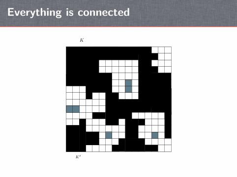
Everything is connected

• Black connector: There exists a connected component of black cellsthat links two opposite sides of [0,1]2.

• Black giant: Black components of size less than 1/r are now recoloredgray. All remaining black cells are connected. The correspondingvertices of G belong to the same connected component.

• Connectivity: Each vertex connects to at least one vertex of the blackgiant.

Everything is connected

K

K ′

Spanning ratio and diameter

An important feature of a geometric graph is the spanning ratio

supi,j

dist(Xi,Xj)

‖Xi−Xj‖

where dist(Xi,Xj) is the shortest (Euclidean) distance of Xi and Xj over theedges of the graph. Ideally, this should be small.

Unfortunately, this can be large if Xi and Xj are very close.However, for c slightly larger than critical, we haveTheorem∃K,µ> 0 such that if γ> γ∗, r= γ

(logn

n

)1/dand c≥µ

√logn then

supi,j:‖Xi−Xj‖>r

dist(Xi,Xj)

‖Xi −Xj‖≤K, whp.



supi,j

dist(Xi,Xj)

‖Xi−Xj‖

where dist(Xi,Xj) is the shortest (Euclidean) distance of Xi and Xj over theedges of the graph. Ideally, this should be small.Unfortunately, this can be large if Xi and Xj are very close.

However, for c slightly larger than critical, we haveTheorem∃K,µ> 0 such that if γ> γ∗, r= γ

(logn

n

)1/dand c≥µ

√logn then


dist(Xi,Xj)




supi,j

dist(Xi,Xj)

‖Xi−Xj‖

where dist(Xi,Xj) is the shortest (Euclidean) distance of Xi and Xj over theedges of the graph. Ideally, this should be small.Unfortunately, this can be large if Xi and Xj are very close.However, for c slightly larger than critical, we haveTheorem∃K,µ> 0 such that if γ> γ∗, r= γ

(logn

n

)1/dand c≥µ

√logn then


dist(Xi,Xj)



This implies that the diameter of G satisfies diam(G)≤Kp

d/r. This isoptimal, up to a constant factor.

Idea of the proof: Partition the unit cube into a grid of cells of side length`= (1/3)

⌊1/r

⌋−1.With high probability, any two points i and j, such that Xi and Xj fall inthe same cell, are connected by a path of length at most five.On the other hand, with high probability, any two neighboring cells containtwo points, one in each cell, that are connected by an edge of Sn.


This implies that the diameter of G satisfies diam(G)≤Kp

d/r. This isoptimal, up to a constant factor.Idea of the proof: Partition the unit cube into a grid of cells of side length`= (1/3)

⌊1/r

⌋−1.With high probability, any two points i and j, such that Xi and Xj fall inthe same cell, are connected by a path of length at most five.On the other hand, with high probability, any two neighboring cells containtwo points, one in each cell, that are connected by an edge of Sn.

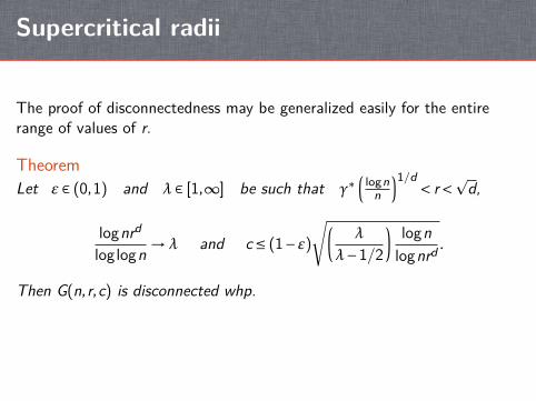
Supercritical radii

The proof of disconnectedness may be generalized easily for the entirerange of values of r.

TheoremLet ε ∈ (0,1) and λ ∈ [1,∞] be such that γ∗

( lognn

)1/d < r<pd,

lognrd

loglogn →λ and c≤ (1−ε)

√(λ

λ−1/2

) lognlognrd .

Then G(n,r,c) is disconnected whp.

In particular, take r∼ n−(1−δ)/d. Then for c≤ (1−ε)/pδ (constant) the

graph is disconnected.

Supercritical r, constant c

We can show that the lower bound is not far from the truth: whenr∼ n−(1−δ)/d, constant c is sufficient for connectivity.c=√

5/δ+c(d) is sufficient for connectivity.The irrigation graph is genuinely sparse.


TheoremLet δ ∈ (0,1), γ> 0. Suppose that rn ∼ γn−(1−δ)/d. There exists a constantc= c(δ,d) such that G is connected whp. One may take c= c1+c2+c3+1,where

c1 = d√

5/(δ−δ2)e ,

and c2,c3 depend on d only.


Sketch of proof:• First show that X1, . . . ,Xn are sufficiently regular whp. Once the Xi arefixed, all randomness comes from the edge choices.

• We add edges in four phases. In the first we start from X1, and using c1choices of each vertex, we go for δ2 logc1 n generations. There exists acube in the grid that contains a connected component of size nconst.δ2 .• Second, we add c2 new connections to each vertex in the component. Atleast one of the grid cells has a positive fraction of its points in aconnected component.• Third, using c3 new connections of each vertex, we obtain a connectedcomponent that contains a constant fraction of the points in every cell ofthe grid, whp.• Finally, add just one more connection per vertex so that the entire graphbecomes connected.


Sketch of proof:• First show that X1, . . . ,Xn are sufficiently regular whp. Once the Xi arefixed, all randomness comes from the edge choices.• We add edges in four phases. In the first we start from X1, and using c1choices of each vertex, we go for δ2 logc1 n generations. There exists acube in the grid that contains a connected component of size nconst.δ2 .

• Second, we add c2 new connections to each vertex in the component. Atleast one of the grid cells has a positive fraction of its points in aconnected component.• Third, using c3 new connections of each vertex, we obtain a connectedcomponent that contains a constant fraction of the points in every cell ofthe grid, whp.• Finally, add just one more connection per vertex so that the entire graphbecomes connected.


Sketch of proof:• First show that X1, . . . ,Xn are sufficiently regular whp. Once the Xi arefixed, all randomness comes from the edge choices.• We add edges in four phases. In the first we start from X1, and using c1choices of each vertex, we go for δ2 logc1 n generations. There exists acube in the grid that contains a connected component of size nconst.δ2 .• Second, we add c2 new connections to each vertex in the component. Atleast one of the grid cells has a positive fraction of its points in aconnected component.

• Third, using c3 new connections of each vertex, we obtain a connectedcomponent that contains a constant fraction of the points in every cell ofthe grid, whp.• Finally, add just one more connection per vertex so that the entire graphbecomes connected.


Sketch of proof:• First show that X1, . . . ,Xn are sufficiently regular whp. Once the Xi arefixed, all randomness comes from the edge choices.• We add edges in four phases. In the first we start from X1, and using c1choices of each vertex, we go for δ2 logc1 n generations. There exists acube in the grid that contains a connected component of size nconst.δ2 .• Second, we add c2 new connections to each vertex in the component. Atleast one of the grid cells has a positive fraction of its points in aconnected component.• Third, using c3 new connections of each vertex, we obtain a connectedcomponent that contains a constant fraction of the points in every cell ofthe grid, whp.

• Finally, add just one more connection per vertex so that the entire graphbecomes connected.


Sketch of proof:• First show that X1, . . . ,Xn are sufficiently regular whp. Once the Xi arefixed, all randomness comes from the edge choices.• We add edges in four phases. In the first we start from X1, and using c1choices of each vertex, we go for δ2 logc1 n generations. There exists acube in the grid that contains a connected component of size nconst.δ2 .• Second, we add c2 new connections to each vertex in the component. Atleast one of the grid cells has a positive fraction of its points in aconnected component.• Third, using c3 new connections of each vertex, we obtain a connectedcomponent that contains a constant fraction of the points in every cell ofthe grid, whp.• Finally, add just one more connection per vertex so that the entire graphbecomes connected.

Thank you

Connectivity of random irrigation...

Documents

Transcript of Connectivity of random irrigation...