Connecting and Visualising Open Data from Multiple Sources
49
Margriet Groenendijk, PhD Developer Advocate for IBM Cloud Data Services Connecting and Visualising Open Data from Multiple Sources Data Driven Innovation Open Summit Rome - 20 May 2016 @MargrietGr
-
Upload
margriet-groenendijk -
Category
Data & Analytics
-
view
115 -
download
5
Transcript of Connecting and Visualising Open Data from Multiple Sources

Margriet Groenendijk, PhDDeveloper Advocate for IBM Cloud Data Services
Connecting and Visualising Open Data from Multiple Sources
Data Driven Innovation Open SummitRome - 20 May 2016
@MargrietGr

Please Note
▪ IBM’s statements regarding its plans, directions, and intent are subject to change or withdrawal without notice at IBM’s sole discretion.
▪ Information regarding potential future products is intended to outline our general product direction and it should not be relied on in making a purchasing decision.
▪ The information mentioned regarding potential future products is not a commitment, promise, or legal obligation to deliver any material, code or functionality. Information about potential future products may not be incorporated into any contract.
▪ The development, release, and timing of any future features or functionality described for our products remains at our sole discretion.
▪ Performance is based on measurements and projections using standard IBM benchmarks in a controlled environment. The actual throughput or performance that any user will experience will vary depending upon many factors, including considerations such as the amount of multiprogramming in the user’s job stream, the I/O configuration, the storage configuration, and the workload processed. Therefore, no assurance can be given that an individual user will achieve results similar to those stated here.
@MargrietGr

About me
• Developer Advocate at IBM Cloud Data Services, UK• Data scientist • Python, R, Cloudant, dashDB
• Research Fellow at University of Exeter, UK• Worked with very large observational datasets and the output of
global scale climate models
• PhD at Vrije Universiteit Amsterdam, the Netherlands• Explored large observational datasets of carbon uptake by forests
@MargrietGr

Outline
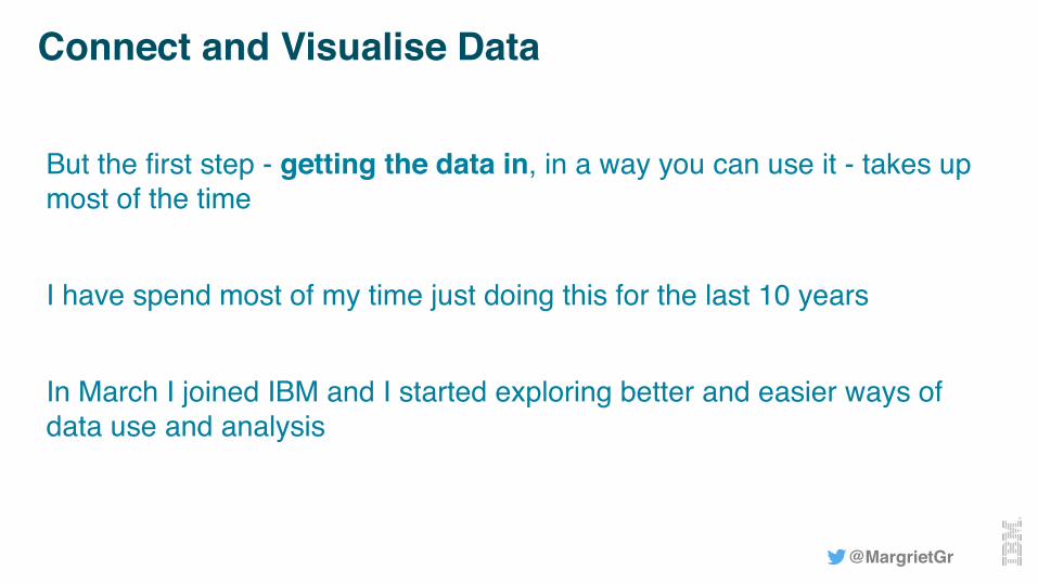
Connect and Visualise Data
@MargrietGr
But the first step - getting the data in, in a way you can use it - takes up most of the time
I have spend most of my time just doing this for the last 10 years
In March I joined IBM and I started exploring better and easier ways of data use and analysis

@MargrietGr
http://geoawesomeness.com/wp-content/uploads/2015/10/GoogeMaps-vs-OSM-Geoawesomeness.jpg
• Freely available• Constantly updated by
local volunteers• Data format needs
some processing

Weather and Climate Data
@MargrietGr
There is a lot of it and the files are large
Binary data format of grids in different shapes and sizes
Clear understanding of where the data comes from is important. Most of it is generated by models or through interpolation of observations

Census Data
@MargrietGr
Demographic, economic an statistical data by country
For US also by state and city
Accessible through APIs

OpenStreetMap Data

OpenStreetMap is built by a community of mappers that contribute and maintain data about roads, trails, cafés, railway stations, and much more, all over the world
Weekly updated
But… large files that can do with some processing to make the data easily accessible
@MargrietGr
https://www.openstreetmap.org
https://www.cloudant.com
use anywhereIBM Cloudant

Several data sources - world, continent, country, city or a user defined box
Several data formats for which free to use conversion tools exist - pbf, osm, json, shp
Example for the Netherlands:
@MargrietGr
wget -c http://download.geofabrik.de/europe/netherlands-latest.osm.pbf
use anywhereIBM Cloudant

Extract the POIs with osmosis
@MargrietGr
osmosis --read-pbf netherlands-latest.osm.pbf \--tf accept-nodes \aerialway=station \aeroway=aerodrome,helipad,heliport \amenity=* craft=* emergency=* \highway=bus_stop,rest_area,services \historic=* leisure=* office=* \ public_transport=stop_position,stop_area \shop=* tourism=* \--tf reject-ways --tf reject-relations \--write-xml netherlands.nodes.osm
(easy to install with brew on Mac)

Some cleaning up with osmconvert
Convert from osm to json format with ogr2ogr
@MargrietGr
osmconvert $netherlands.nodes.osm --drop-ways --drop-author --drop-relations --drop-versions >$netherlands.poi.osm
ogr2ogr -f GeoJSON $netherlands.poi.json $netherlands.poi.osm points

Create an account on www.cloudant.com(free trial available)
Upload to Cloudant with couchimport
@MargrietGr
export COUCH_URL="https://username:[email protected]"
cat $netherlands.poi.json | couchimport --db poi-$netherlands --type json --jsonpath "features.*"
https://github.com/glynnbird/couchimport
IBM Cloudant
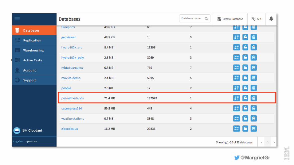
▪ Cloudant screen shot…
@MargrietGr

▪ Cloudant screen shot…
@MargrietGr

▪ Cloudant screen shot…
@MargrietGr
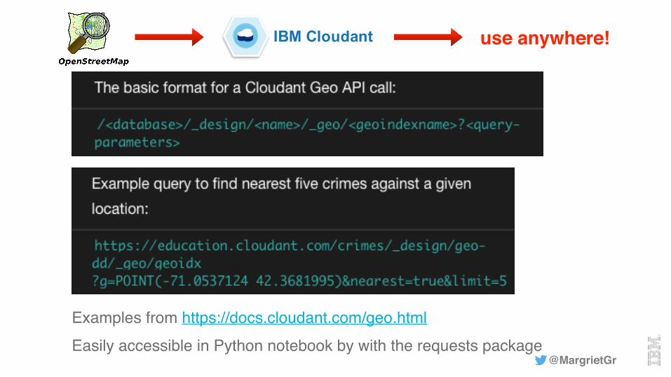
Examples from https://docs.cloudant.com/geo.htmlEasily accessible in Python notebook by with the requests package
@MargrietGr
use anywhere!IBM Cloudant

@MargrietGr
use anywhereIBM Cloudant
Weekly updates
Adapt the code and automate it to run weekly
Up to date database

Weather and Climate Data

Weather and Climate Data
@MargrietGr
There is a lot of it and the files are large
Binary data format of grids in different shapes and sizes
http://www.cru.uea.ac.uk/data/
https://modelingguru.nasa.gov/docs/DOC-2312

https://developer.ibm.com/clouddataservices/2016/04/18/predict-temperatures-using-dashdb-python-and-r/
@MargrietGr
Weather and Climate Data
The below blog explains how to process some example data and load it into a relation database (dashDB) This data is now easily accessible

Load data into Python directly from dashDB(credentials are easily found in dashDB)
@MargrietGr
from ibmdpy import IdaDataBase, IdaDataFrame
jdbc = "jdbc:db2://dashdb-entry-yp-dal09-09.services.dal.bluemix.net:50000/BLUDB:user=" + username + ";password=" + password
idadb = IdaDataBase(jdbc)

@MargrietGr
Average global temperature
import pandas as pd
temp = pd.read_csv("temperature.csv")
temp[0:5]
@MargrietGr
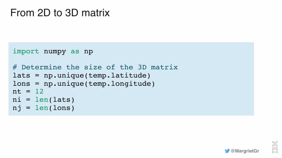
From 2D to 3D matrix
import numpy as np
# Determine the size of the 3D matrixlats = np.unique(temp.latitude)lons = np.unique(temp.longitude)nt = 12ni = len(lats) nj = len(lons)

@MargrietGr
From 2D to 3D matrix# Create and fill matrix by looping over the 3 dimensionstemperature = np.zeros(nt*ni*nj) temperature.shape = [nt, ni, nj] mo = -1for mon in range(1,13): mo = mo+1 la = -1 for lat in lats: la = la+1 lo = -1 for lon in lons: lo = lo+1 t = temp["temperature"][(temp["month"]==mon) & (temp["latitude"]==lat) & (temp["longitude"]==lon)] temperature[mo, la, lo] = np.array(t)

@MargrietGr
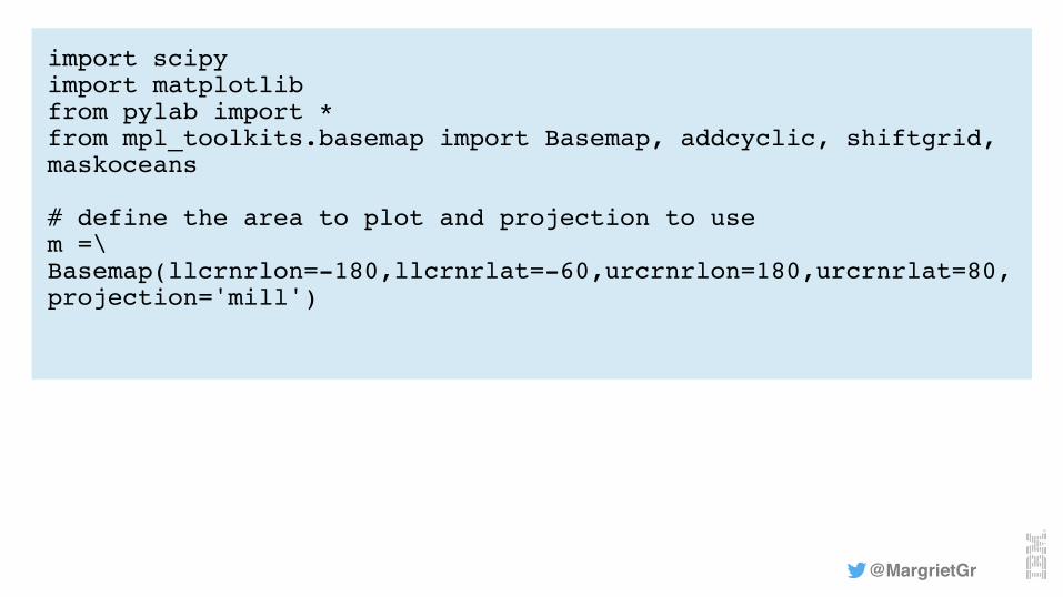
import scipyimport matplotlibfrom pylab import *from mpl_toolkits.basemap import Basemap, addcyclic, shiftgrid, maskoceans
@MargrietGr
import scipyimport matplotlibfrom pylab import *from mpl_toolkits.basemap import Basemap, addcyclic, shiftgrid, maskoceans
# define the area to plot and projection to usem =\Basemap(llcrnrlon=-180,llcrnrlat=-60,urcrnrlon=180,urcrnrlat=80,projection='mill')

@MargrietGr
Global temperature mapimport scipyimport matplotlibfrom pylab import *from mpl_toolkits.basemap import Basemap, addcyclic, shiftgrid, maskoceans
# define the area to plot and projection to usem =\Basemap(llcrnrlon=-180,llcrnrlat=-60,urcrnrlon=180,urcrnrlat=80,projection='mill')
# covert the latitude, longitude and temperatures to raster coordinates to be plottedt1=temperature[0,:,:]t1,lon=addcyclic(t1,lons)january,longitude=shiftgrid(180.,t1,lon,start=False)x,y=np.meshgrid(longitude,lats)px,py=m(x,y)

@MargrietGr
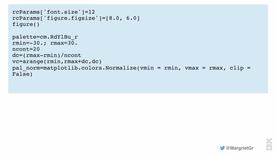
rcParams['font.size']=12rcParams['figure.figsize']=[8.0, 6.0]figure()
@MargrietGr
rcParams['font.size']=12rcParams['figure.figsize']=[8.0, 6.0]figure()
palette=cm.RdYlBu_rrmin=-30.; rmax=30.ncont=20 dc=(rmax-rmin)/ncontvc=arange(rmin,rmax+dc,dc) pal_norm=matplotlib.colors.Normalize(vmin = rmin, vmax = rmax, clip = False)

@MargrietGr
Global temperature maprcParams['font.size']=12rcParams['figure.figsize']=[8.0, 6.0]figure()
palette=cm.RdYlBu_rrmin=-30.; rmax=30.ncont=20 dc=(rmax-rmin)/ncontvc=arange(rmin,rmax+dc,dc) pal_norm=matplotlib.colors.Normalize(vmin = rmin, vmax = rmax, clip = False)
m.drawcoastlines(linewidth=0.5)m.drawmapboundary(fill_color=(1.0,1.0,1.0))cf=m.pcolormesh(px, py, january, cmap = palette)cbar=colorbar(cf,orientation='horizontal', shrink=0.95)cbar.set_label('Mean Temperature in January')
tight_layout()
show()

@MargrietGr

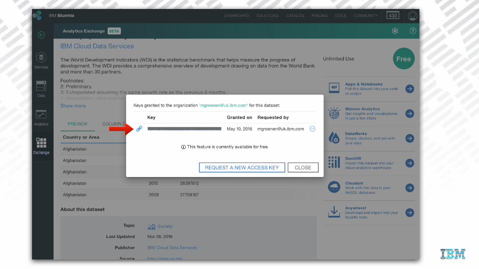
UN Census datahttps://console.ng.bluemix.net/data/exchange

Census Data
@MargrietGr
Demographic, economic an statistical data by country
For US also by state and city
Accessible through APIs

36

37

@MargrietGr

39

40
41
——————————

@MargrietGr
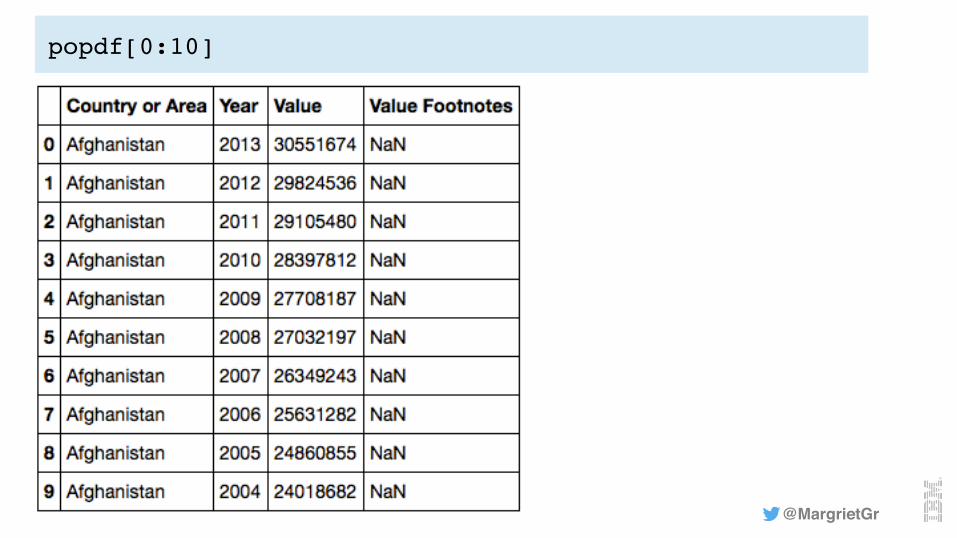
import urllib
filelink=urllib.urlopen(“https://console.ng.bluemix.net/data/exchange-api/v1/entries/889ca053a19986a4445839358a91963e/data?accessKey=xxxxxx")
popdf = pd.read_csv(filelink)
list(popdf)
['Country or Area', 'Year', 'Value', 'Value Footnotes']
@MargrietGr
popdf[0:10]

Combine and visualise

Combine and Visualise
▪ POI data in Cloudant▪ Weather data in dashDB▪ Census data
@MargrietGr

In the cloud: Data & Analytics on IBM Bluemix
@MargrietGr

Key points
▪ There is lots of data freely available ▪ A lot of analysis tools are free, with examples in blogs and on Github▪ There is still lots of preparation needed before doing any analysis or visualisation▪ But this getting easier and easier
▪ API access of data▪ Data storage, analysis and visualisation in the cloud
@MargrietGr

https://github.com/MargrietGroenendijk/notebooks
Thank you!
@MargrietGr
Margriet GroenendijkDeveloper Advocate for IBM Cloud Data Services