Conformal Field Theory and Statistical Mechanics · Conformal Field Theory and Statistical...

Conformal Field Theory and Statistical Mechanics∗

John Cardy

July 2008

∗Lectures given at the Summer School on Exact methods in low-dimensional statistical physics andquantum computing, les Houches, July 2008.

1

CFT and Statistical Mechanics 2

Contents

1 Introduction 3

2 Scale invariance and conformal invariance in critical behaviour 3

2.1 Scale invariance . . . . . . . . . . . . . . . . . . . . . . . . . . . . . . . . . 3

2.2 Conformal mappings in general . . . . . . . . . . . . . . . . . . . . . . . . 6

3 The role of the stress tensor 7

3.0.1 An example - free (gaussian) scalar field . . . . . . . . . . . . . . . 8

3.1 Conformal Ward identity . . . . . . . . . . . . . . . . . . . . . . . . . . . . 9

3.2 An application - entanglement entropy . . . . . . . . . . . . . . . . . . . . 12

4 Radial quantisation and the Virasoro algebra 14

4.1 Radial quantisation . . . . . . . . . . . . . . . . . . . . . . . . . . . . . . . 14

4.2 The Virasoro algebra . . . . . . . . . . . . . . . . . . . . . . . . . . . . . . 15

4.3 Null states and the Kac formula . . . . . . . . . . . . . . . . . . . . . . . . 16

4.4 Fusion rules . . . . . . . . . . . . . . . . . . . . . . . . . . . . . . . . . . . 17

5 CFT on the cylinder and torus 18

5.1 CFT on the cylinder . . . . . . . . . . . . . . . . . . . . . . . . . . . . . . 18

5.2 Modular invariance on the torus . . . . . . . . . . . . . . . . . . . . . . . . 20

5.2.1 Modular invariance for the minimal models . . . . . . . . . . . . . . 22

6 Height models, loop models and Coulomb gas methods 24

6.1 Height models and loop models . . . . . . . . . . . . . . . . . . . . . . . . 24

6.2 Coulomb gas methods . . . . . . . . . . . . . . . . . . . . . . . . . . . . . 27

6.3 Identification with minimal models . . . . . . . . . . . . . . . . . . . . . . 28

7 Boundary conformal field theory 29

7.1 Conformal boundary conditions and Ward identities . . . . . . . . . . . . . 29

7.2 CFT on the annulus and classification of boundary states . . . . . . . . . . 30

7.2.1 Example . . . . . . . . . . . . . . . . . . . . . . . . . . . . . . . . . 34


7.3 Boundary operators and SLE . . . . . . . . . . . . . . . . . . . . . . . . . 34

8 Further Reading 37

1 Introduction

It is twenty years ago almost to the day that the les Houches school on Fields, Strings andCritical Phenomena took place. It came on the heels of a frenzied period of five years orso following the seminal paper of Belavin, Polyakov and Zamolodchikov (BPZ) in whichthe foundations of conformal field theory and related topics had been laid down, andfeatured lectures on CFT by Paul Ginsparg, Ian Affleck, Jean-Bernard Zuber and myself,related courses and talks by Hubert Saleur, Robert Dijkgraaf, Bertrand Duplantier, SashaPolyakov, Daniel Friedan, as well as lectures on several other topics. The list of youngparticipants, many of whom have since gone on to make their own important contributions,is equally impressive.

Twenty years later, CFT is an essential item in the toolbox of many theoretical condensedmatter physicists and string theorists. It has also had a marked impact in mathematics, inalgebra, geometry and, more recently, probability theory. It is the purpose of these lecturesto introduce some of these tools. In some ways they are an updated version of those Igave in 1988. However, there are some important topics there which, in order to includenew material, I will omit here, and I would encourage the diligent student to read bothversions. I should stress that the lectures will largely be about Conformal Field Theory,rather than Conformal Field Theories, in the sense that I’ll be describing rather genericproperties of CFT rather than discussing particular examples. That said, I don’t want thediscussion to be too abstract, and in fact I will have a very specific idea about what are thekind of CFTs I will be discussing: the scaling limit (in a sense to be described) of criticallattice models (either classical, in two dimensions, or quantum in 1+1 dimensions.) Thiswill allow us to have, I hope, more concrete notions of the mathematical objects whichare being discussed in CFT. However there will be no attempt at mathematical rigour.Despite the fact that CFT can be developed axiomatically, I think that for this audienceit is more important to understand the physical origin of the basic ideas.

2 Scale invariance and conformal invariance in criti-

cal behaviour

2.1 Scale invariance

The prototype lattice model we have at the back of our minds is the ferromagnetic Isingmodel. We take some finite domain D of d-dimensional euclidean space and impose a


regular lattice, say hypercubic, with lattice constant a. With each node r of the latticewe associate a binary-valued spin s(r) = ±1. Each configuration {s} carries a relativeweight W ({s}) ∝ exp(

∑rr′∈D J(r− r′)s(r)s(r)) where J(r− r′) > 0 is some short-ranged

interaction (i.e. it vanishes if |r − r′| is larger than some fixed multiple of a.)

The usual kinds of local observable φlatj (r) considered in this lattice model are sums of

products of nearby spins over some region of size O(a), for example the local magnetisations(r) itself, or the energy density

∑r′ J(r− r′)s(r)s(r′). However it will become clear later

on that there are other observables, also labelled by a single point r, which are functionsof the whole configuration {s}. For example, we shall show that this Ising model canbe mapped onto a gas of non-intersecting loops. An observable then might depend onwhether a particular loop passes through the given point r. From the point of view ofCFT, these observables are equally valid objects.

Correlation functions, that is expectation values of products of local lattice observables,are then given by

〈φlat1 (r1)φlat

2 (r2) . . . φlatn (rn)〉 = Z−1

∑{s}

φlat1 (r1) . . . φlat

n (rn)W ({s}) ,

where Z =∑{s}W ({s}) is the partition function. In general, the connected pieces of these

correlations functions fall off over the same distance scale as the interaction J(r−r′), but,close to a critical point, this correlation length ξ can become large, � a.

The scaling limit is obtained by taking a → 0 while keeping ξ and the domain D fixed.In general the correlation functions as defined above do not possess a finite scaling limit.However, the theory of renormalisation (based on studies in exactly solved models, as wellas perturbative analysis of cut-off quantum field theory) suggests that in general thereare particular linear combinations of local lattice observables which are multiplicativelyrenormalisable. That is, the limit

lima→0

a−∑n

j=1xj〈φlat

1 (r1)φlat2 (r2) . . . φlat

n (rn)〉 (1)

exists for certain values of the {xj}. We usually denote this by

〈φ1(r1)φ2(r2) . . . φn(rn)〉 , (2)

and we often think of it as the expectation value of the product the random variablesφj(rj), known as scaling fields (sometimes scaling operators, to be even more confusing)with respect to some ‘path integral’ measure. However it should be stressed that thisis only an occasionally useful fiction, which ignores all the wonderful subtleties of renor-malised field theory. The basic objects of QFT are the correlation functions. The numbers{xj} in (1) are called the scaling dimensions.

One important reason why this is not true in general is that the limit in (1) in fact onlyexists if the points {rj} are non-coincident. The correlation functions in (2) are singular


in the limits when ri → rj. However, the nature of these singularities is prescribed by theoperator product expansion (OPE)

〈φi(ri)φj(rj) . . .〉 =∑k

Cijk(ri − rj)〈φk((ri + rj)/2) . . .〉 . (3)

The main point is that, in the limit when |ri−rj| is much less than the separation betweenri and all the other arguments in . . ., the coefficients Cijk are independent of what is inthe dots. For this reason, (3) is often written as

φi(ri) · φj(rj) =∑k

Cijk(ri − rj)φk((ri + rj)/2) , (4)

although it should be stressed that this is merely a short-hand for (3).

So far we have been talking about how to get a continuum (euclidean) field theory asthe scaling limit of a lattice model. In general this will be a massive QFT, with a massscale given by the inverse correlation length ξ−1. In general, the correlation functions willdepend on this scale. However, at a (second-order) critical point the correlation length ξdiverges, that is the mass vanishes, and there is no length scale in the problem besidesthe overall size L of the domain D.

The fact that the scaling limit of (1) exists then implies that, instead of starting with alattice model with lattice constant a, we could equally well have started with one withsome fraction a/b. This would, however, be identical with a lattice model with the originalspacing a, in which all lengths (including the size of the domain D) are multiplied by b.This implies that the correlation functions in (2) are scale covariant:

〈φ1(br1)φ2(br2) . . . φn(brn)〉bD = b−∑

jxj〈φ1(r1)φ2(r2) . . . φn(rn)〉D . (5)

Once again, we can write this in the suggestive form

φj(br) = b−xjφj(r) , (6)

as long as what we really mean is (5).

In a massless QFT, the form of the OPE coefficients in (4) simplifies: by scale covariance

Cijk(rj − rk) =cijk

|ri − rj|xi+xj−xk, (7)

where the cijk are pure numbers, and universal if the 2-point functions are normalised sothat 〈φj(r1)φj(r2)〉 = |r1− r2|−2xj . (This assumes that the scaling fields are all rotationalscalars – otherwise it is somewhat more complicated, at least for general dimension.)

From scale covariance, it is a simple but powerful leap to conformal covariance: supposethat the scaling factor b in (5) is a slowly varying function of position r. Then we can tryto write a generalisation of (5) as

〈φ1(r′1)φ2(r′2) . . . φn(r′n)〉D′ =n∏j=1

b(rj)−xj〈φ1(r1)φ2(r2) . . . φn(rn)〉D , (8)


where b(r) = |∂r′/∂r| is the local jacobian of the transformation r → r′.

For what transformations r → r′ do we expect (8) to hold? The heuristic argument runsas follows: if the theory is local (that is the interactions in the lattice model are short-ranged), then as long as the transformations looks locally like a scale transformation (plusa possible rotation), then (8) may be expected to hold. (In Sec. 3 we will make this moreprecise, based on the assumed properties of the stress tensor, and argue that in fact itholds only for a special class of scaling fields {φj} called primary.)

It is most important that the underlying lattice does not transform (otherwise the state-ment is a tautology): (8) relates correlation functions in D, defined in terms of the limita→ 0 of a model on a regular lattice superimposed on D, to correlation functions definedby a regular lattice superimposed on D′.

Transformations which are locally equivalent to a scale transformation and rotation, thatis, have no local components of shear, also locally preserve angles and are called conformal.

2.2 Conformal mappings in general

Consider a general infinitesimal transformation (in flat space) rµ → r′µ = rµ + αµ(r)(we distinguish upper and lower indices in anticipation of using coordinates in which themetric is not diagonal.) The shear component is the traceless symmetric part

αµ,ν + αν,µ − (2/d)αλ,λgµν ,

all 12d(d+ 1)− 1 components of which must vanish for the mapping to be conformal. For

general d this is very restrictive, and in fact, apart from uniform translations, rotationsand scale transformations, there is only one other type of solution

αµ(r) = bµr2 − 2(b · r)rµ ,where bµ is a constant vector. These are in fact the composition of the finite conformalmapping of inversion rµ → rµ/|r|2, followed by an infinitesimal translation bµ, followed bya further inversion. They are called the special conformal transformations, and togetherwith the others, they generate a group isomorphic to SO(d+ 1, 1).

These special conformal transformations have enough freedom to fix the form of the 3-point functions in Rd (just as scale invariance and rotational invariance fixes the 2-pointfunctions): for scalar operators1

〈φ1(r1)φ2(r2)φ3(r3)〉 =c123

|r1 − r2|x1+x2−x3|r2 − r3|x2+x3−x1|r3 − r1|x3+x1−x2. (9)

Comparing with the OPE (4,7), and assuming non-degeneracy of the scaling dimensions2,we see that c123 is the same as the OPE coefficient defined earlier. This shows that theOPE coefficients cijk are symmetric in their indices.

1The easiest way to show this it to make an inversion with an origin very close to one of the points,say r1, and then use the OPE, since its image is then very far from those of the other two points.

2This and other properties fail in so-called logarithmic CFTs.


In two dimensions, the condition that αµ(r) be conformal imposes only two differentialconditions on two functions, and there is a much wider class of solutions. These are moreeasily seen using complex coordinates3 z ≡ r1 + ir2, z ≡ r1 − ir2, so that the line elementis ds2 = dzdz, and the metric is

gµν =(

0 12

12

0

)gµν =

(0 22 0

).

In this basis, two of the conditions are satisfied identically and the others become

αz,z = αz,z = 0 ,

which means that ∂αz/∂z = ∂αz/∂z = 0, that is, αz is a holomorphic function α(z) of z,and αz is an antiholomorphic function.

Generalising this to a finite transformation, it means that conformal mappings r → r′

correspond to functions z → z′ = f(z) which are analytic in D. (Note that the onlysuch functions on the whole Riemann sphere are the Mobius transformations f(z) =(az + b)/(cz + d), which are the finite special conformal mappings.)

In passing, let us note that complex coordinates give us a nice way of discussing non-scalar fields: if, for example, under a rotation z → zeiθ, φj(z, z)→ eisjθφj, we say that φjhas conformal spin sj (not related to quantum mechanical spin), and under a combinedtransformation z → λz where λ = beiθ we can write (in the same spirit as (6))

φj(λz, λz) = λ−∆j λ−∆jφj(z, z) ,

where xj = ∆j + ∆j, sj = ∆j −∆j. (∆j,∆j) are called the complex scaling dimensions ofφj (although they are usually both real, and not necessarily complex conjugates of eachother.)

3 The role of the stress tensor

Since we wish to explore the consequences of conformal invariance for correlation func-tions in a fixed domain D (usually the entire complex plane), it is necessary to considertransformations which are not conformal everywhere. This brings in the stress tensor Tµν(also known as the stress-energy tensor or the (improved) energy-momentum tensor). Itis the object appearing on the right hand side of Einstein’s equations in curved space. Ina classical field theory, it is defined in terms of the response of the action S to a generalinfinitesimal transformation αµ(r):

δS = − 1

2π

∫Tµνα

µ,νd2r (10)

3For many CFT computations we may treat z and z as independent, imposing only at the end thatthey should be complex conjugates.


(the (1/2π) avoids awkward such factors later on.) Invariance of the action under trans-lations and rotations implies that Tµν is conserved and symmetric. Moreover if S is scaleinvariant, Tµν is also traceless. In complex coordinates, the first two conditions imply thatTzz + Tzz = 0 and Tzz = Tzz, so they both vanish, and the conservation equations thenread ∂zTzz = 2∂Tzz/∂z = 0 and ∂Tzz/∂z = 0. Thus the non-zero components T ≡ Tzzand T ≡ Tzz are respectively holomorphic and antiholomorphic fields. Now if we considera more general transformation for which αµ,ν is symmetric and traceless, that is a confor-mal transformation, we see that δS = 0 in this case also. Thus, at least classically, we seethat scale invariance and rotational invariance imply conformal invariance of the action,at least if (10) holds. However if the theory contains long-range interactions, for example,this is no longer the case.

In a quantum 2d CFT, it is assumed that the above analyticity properties continue tohold at the level of correlation functions: those of T (z) and T (z) are holomorphic andantiholomorphic functions of z respectively (except at coincident points.)

3.0.1 An example - free (gaussian) scalar field

The prototype CFT is the free, or gaussian, massless scalar field h(r) (we use this notationfor reasons that will emerge later). It will turn out that many other CFTs are basicallyvariants of this. The classical action is

S[h] = (g/4π)∫

(∂µh)(∂µh)d2r .

Since h(r) can take any real value, we could rescale it to eliminate the coefficient in front,but in later extensions this will have a meaning, so we keep it. In complex coordinates,S ∝

∫(∂zh)(∂zh)d2z, and it is easy to see that this is conformally invariant under z →

z′ = f(z), since ∂z = f ′(z)∂z′ , ∂z = f ′(z)∂z′ and d2z = |f ′(z)|−2d2z′. This is confirmed bycalculating Tµν explicitly: we find Tzz = Tzz = 0, and

T = Tzz = −g(∂zh)2, T = Tzz = −g(∂zh)2 .

These are holomorphic (resp. antiholomorphic) by virtue of the classical equation of mo-tion ∂z∂zh = 0.

In the quantum field theory, a given configuration {h} is weighted by exp(−S[h]). The2-point function is4

〈h(z, z)h(0, 0)〉 =2π

g

∫ eik·r

k2

d2k

(2π)2∼ −(1/2g) log(zz/L2) .

This means that 〈T 〉 is formally divergent. It can be made finite, for example, by point-splitting and subtracting off the divergent piece:

T (z) = −g limδ→0

(∂zh(z + 1

2δ)∂zh(z − 1

2δ)− 1

2gδ2

). (11)

4this is cut-off at small k by the assumed finite size L, but we are here also assuming that the pointsare far from the boundary.


C

D

Figure 1: We consider an infinitesimal transformation which is conformal within C and theidentity in the complement in D.

This doesn’t affect the essential properties of T .

3.1 Conformal Ward identity

Consider a general correlation function of scaling fields 〈φ1(z1, z1)φ2(z2, z2) . . .〉D in somedomain D. We want to make an infinitesimal conformal transformation z → z′ = z+α(z)on the points {zj}, without modifying D. This can be done by considering a contour Cwhich encloses all the points {zj} but which lies wholly within D, such that the trans-formation is conformal within C, and the identity z′ = z outside C (Fig. 1). This givesrise to an (infinitesimal) discontinuity on C, and, at least classically to a modification ofthe action S according to (10). Integrating by parts, we find δS = (1/2π)

∫C Tµνα

µnνd`,where nν is the outward-pointing normal and d` is a line element of C. This is more easilyexpressed in complex coordinates, after some algebra, as

δS =1

2πi

∫Cα(z)T (z)dz + complex conjugate .

This extra factor can then be expanded, to first order in α, out of the weight exp(−S[h]−δS) ∼ (1 − δS) exp(−S[h]), and the extra piece δS considered as an insertion into thecorrelation function. This is balanced by the explicit change in the correlation functionunder the conformal transformation:

δ〈φ1(z1, z1)φ2(z2, z2) . . .〉 =1

2πi

∫Cα(z)〈T (z)φ1(z1, z1)φ2(z2, z2) . . .〉dz + c.c. (12)

Let us first consider the case when α(z) = λ(z − z1), that is corresponds to a combinedrotation and scale transformation. In that case δφ1 = (∆1λ + ∆1λ)φ1, and therefore,equating coefficients of λ and λ,∫

C(z − z1)〈T (z)φ1(z1, z1)φ2(z2, z2) . . .〉 dz

2πi= ∆1〈φ1(z1, z1)φ2(z2, z2) . . .〉+ · · · .


Similarly, if we take α = constant, corresponding to a translation, we have δφj ∝ ∂zjφj,so ∫

C〈T (z)φ1(z1, z1)φ2(z2, z2) . . .〉 dz

2πi=∑j

∆j∂zj〈φ1(z1, z1)φ2(z2, z2) . . .〉 .

Using Cauchy’s theorem, these two equations tell us about two of the singular terms inthe OPE of T (z) with a general scaling field φj(zj, zj):

T (z) · φj(zj, zj) = · · ·+ ∆j

(z − zj)2φj(zj, zj) +

1

z − zj∂zjφj(zj, zj) + · · · . (13)

Note that only integer powers can occur, because the correlation function is a meromorphicfunction of z.

Example of the gaussian free field. If we take φlatq (r) = eiqh(r) then

〈φlatq (r1)φlat

−q(r2)〉 = exp (− 12q2〈(h(r1)− h(r2))2〉) ∼

(a

|r1 − r2|

)q2/g

,

which means that the renormalised field φq ∼ a−q2/2gφlat

q has scaling dimension xq = q2/2g.It is then a nice exercise in Wick’s theorem to check that the OPE with the stress tensor(13) holds with ∆q = xq/2. (Note that in this case the multiplicative renormalisation ofφq is equivalent to ignoring all Wick contractions between fields h(r) at the same point.)

Now suppose each φj is such that the terms O((z−zj)−2−n) with n ≥ 1 in (13) are absent.Since a meromorphic function is determined entirely by its singularities, we then knowthe correlation function 〈T (z) . . .〉 exactly:

〈T (z)φ1(z1, z1)φ2(z2, z2) . . .〉 =∑j

(∆j

z − zj)2+

1

z − zj∂zj

)〈φ1(z1, z1)φ2(z2, z2) . . .〉 . (14)

This (as well as a similar equation for an insertion of T ) is the conformal Ward identity.We derived it assuming that the quantum theory could be defined by a path integral andthe change in the action δS follows the classical pattern. For a more general CFT, notnecessarily ‘defined’ (however loosely) by a path integral, (14) is usually assumed as aproperty of T . In fact many basic introductions to CFT use this as a starting point.

Scaling fields φj(zj, zj) such that the most singular term in their OPE with T (z) is O((z−zj)−2) are called primary.5 All the other fields like those appearing in the less singular

terms in (13) are called descendants. Once one knows the correlation functions of all theprimaries, those of the rest follow from (13).6

For correlations of such primary fields, we can now reverse the arguments leading to (13)for the case of a general infinitesimal conformal transformation α(z) and conclude that

δ〈φ1(z1, z1)φ2(z2, z2) . . .〉 =∑j

(∆jα′(zj) + α(zj)∂zj)〈φ1(z1, z1)φ2(z2, z2) . . .〉 ,

5If we assume that there is a lower bound to the scaling dimensions, such fields must exist.6Since the scaling dimensions of the descendants differ from those of the corresponding primaries by

positive integers, they are increasingly irrelevant in the sense of the renormalisation group.


which may be integrated up to get the result for a finite conformal mapping z → z′ = f(z):

〈φ1(z1, z1)φ2(z2, z2) . . .〉D =∏j

f ′(zj)∆jf ′(zj)

∆j〈φ1(z′1, z′1)φ2(z′2, z

′2) . . .〉D′ .

This is just the result we wanted to postulate in (8), but now we see that it can hold onlyfor correlation functions of primary fields.

It is important to realise that T itself is not in general primary. Indeed its OPE withitself must take the form7

T (z) · T (z1) =c/2

(z − z1)4+

2

(z − z1)2T (z1) +

1

z − z1

∂z1T (z1) · · · . (15)

This is because (taking the expectation value of both sides) the 2-point function 〈T (z)T (z1)〉is generally non-zero. Its form is fixed by the fact that ∆T = 2, ∆T = 0, but, since thenormalisation of T is fixed by its definition (10), its coefficient c/2 is fixed. This intro-duces the conformal anomaly number c, which is part of the basic data of the CFT, alongwith the scaling dimensions (∆j,∆j) and the OPE coefficients cijk.

8

This means that, under an infinitesimal transformation α(z), there is an additional termin the transformation law of T :

δT (z) = 2α′(z)T (z) + α(z)∂zT (z) + c12α′′′(z) .

For a finite conformal transformation z → z′ = f(z), this integrates up to

T (z) = f ′(z)2T (z′) + c12{z′, z} , (16)

where the last term is the Schwarzian derivative

{w(z), z} =w′′′(z)w′(z)− 3

2w′′(z)2

w′(z)2.

The form of the Schwarzian can be seen most easily in the example of a gaussian free field.In this case, the point-split terms in (11) transform properly and give rise to the first termin (16), but the fact that the subtraction has to be made separately in the origin frameand the transformed one leads to an anomalous term

limδ→0

g

(f ′(z + 1

2δ)f ′(z − 1

2δ)

2g(f(z + 12δ)− f(z − 1

2δ))2 −

1

2gδ2

),

which, after some algebra, gives the second term in (16) with c = 1.9

7The O((z − z1)−3) term is absent by symmetry under exchange of z and z1.8When the theory is placed in curved background, the trace 〈Tµµ 〉 ∝ cR, where R is the local scalar

curvature.9This is a classic example of an anomaly in QFT, which comes about because the regularisation

procedure does not respect a symmetry.


=1Z

(

β

τ

x0

φ

φ ,φ )ρ

φ

Figure 2: The density matrix is given by the path integral over a space-time region in whichthe rows and columns are labelled by the initial and final values of the fields.

3.2 An application - entanglement entropy

Let’s take a break from the development of the general theory and discuss how the con-formal anomaly number c arises in an interesting (and topical) physical context. Sup-pose that we have a massless relativistic quantum field theory in 1+1 dimensions, whoseimaginary time behaviour therefore corresponds to a euclidean CFT. (There are manycondensed matter systems whose large distance behaviour is described by such a theory.)The system is at zero temperature and therefore in its ground state |0〉, corresponding toa density matrix ρ = |0〉〈0|. Suppose an observer A has access to just part of the system,for example a segment of length ` inside the rest of the system, of total length L � `,observed by B. The measurements of A and B are entangled. It can be argued that auseful measure of the degree of entanglement is the entropy SA = −TrA ρA log ρA, whereρA = TrB ρ is the reduced density matrix corresponding to A.

How can we calculate SA using CFT methods? The first step is to realise that if we cancompute Tr ρnA for positive integer n, and then analytically continue in n, the derivative∂/∂n|n=1 will give the required quantity. For any QFT, the density matrix at finite inversetemperature β is given by the path integral over some fundamental set of fields h(x, t) (tis imaginary time)

ρ({h(x, 0)}, {h(x, β)}) = Z−1∫ ′

[dh(x, t)]e−S[h] ,

where the rows and columns of ρ are labelled by the values of the fields at times 0 and βrespectively, the the path integral is over all histories h(x, t) consistent with these initialand final values (Fig. 2). Z is the partition function, obtained by sewing together theedges at these two times, that is setting h(x, β) = h(x, 0) and integrating

∫[dh(x, 0)].

We are interested in the partial density matrix ρA, which is similarly found by sewingtogether the top and bottom edges for x ∈ B, that is, leaving open a slit along theinterval A (Fig. 3). The rows and columns of ρA are labelled by the values of the fields onthe edges of the slit. Tr ρnA is then obtained by sewing together the edges of n copies ofthis slit cylinder in a cyclic fashion (Fig. 4). This gives an n-sheeted surface with branch


ρA

=1

ZA

Figure 3: The reduced density matrix ρA is given by the path integral over a cylinder with aslit along the interval A.

Figure 4: Tr ρnA corresponds to sewing together n copies so that the edges are connected cycli-cally.

points, or conical singularities, at the ends of the interval A. If Zn is the partition functionon this surface, then

Tr ρnA = Zn/Zn1 .

Let us consider the case of zero temperature, β → ∞, when the whole system is in theground state |0〉. If the ends of the interval are at (x1, x2), the conformal mapping

z =(w − x1

w − x2

)1/n

maps the n-sheeted w-surface to the single-sheeted complex z-plane. We can use thetransformation law (16) to compute 〈T (w)〉, given that 〈T (z)〉 = 0 by translational androtational invariance. This gives, after a little algebra,

〈T (w)〉 =(c/12)(1− 1/n2)(x2 − x1)2

(w − x1)2(w − x2)2.

Now suppose we change the length ` = |x2 − x1| slightly, by making an infinitesimalnon-conformal transformation x→ x+ δ`δ(x− x0), where x1 < x0 < x2. The response ofthe log of the partition function, by the definition of the stress tensor, is

δ logZn = −nδ`2π

∫ ∞−∞〈Txx(x0, t)〉dt

(the factor n occurs because it has to be inserted on each of the n sheets.) WritingTxx = T + T , the integration in each term can be carried out by wrapping the contouraround either of the points x1 or x2. The result is

∂ logZn∂`

= −(c/6)(n− 1/n)

`,

so that Zn/Zn1 ∼ `−(c/6)(n−1/n). Taking the derivative with respect to n at n = 1 we get

the final resultSA ∼ (c/3) log ` .


Figure 5: The state |φj〉 is defined by weighting field configurations on the circle with the pathintegral inside, with an insertion of the field φj(0) at the origin.

4 Radial quantisation and the Virasoro algebra

4.1 Radial quantisation

Like any quantum theory CFT can be formulated in terms of local operators acting on aHilbert space of states. However, as it is massless, the usual quantisation of the theory onthe infinite line is not so useful since it is hard to disentangle the continuum of eigenstatesof the hamiltonian, and we cannot define asymptotic states in the usual way. Instead itis useful to exploit the scale invariance, rather than the time-translation invariance, andquantise on a circle of fixed radius r0. In the path integral formulation, heuristically theHilbert space is the space of field configurations |{h(r0, θ)}〉 on this circle. The analogueof the hamiltonian is then the generator D of scale transformations. It will turn out thatthe spectrum of D is discrete. In the vacuum state each configuration is weighted by thepath integral over the disc |z| < r0, conditioned on taking the assigned values on r0, seeFig. 5:

|0〉 =∫

[dh(r ≤ r0)]e−S[h]|{h(r0, θ)}〉 .

The scale invariance of the action means that this state is independent of r0, up to aconstant. If instead we insert a scaling field φj(0) into the above path integral, we geta different state |φj〉. On the other hand, more general correlation functions of scalingfields are given in this operator formalism by10

〈φj(z1, z1)φj(z2, z2)〉 = 〈0|R φj(z1, z1)φj(z2, z2)|0〉 ,

where R means the r-ordered product (like the time-ordered product in the usual case),and 〈0| is defined similarly in terms of the path integral over r > r0. Thus we can identify

|φj〉 = limz→0

φj(z, z)|0〉 .

This is an example of the operator-state correspondence in CFT.

10We shall make an effort consistently to denote actual operators (as opposed to fields) with a hat.


Just as the hamiltonian in ordinary QFT can be written as an integral over the appropriatecomponent of the stress tensor, we can write

D = L0 + L0 ≡1

2πi

∫CzT (z)dz + c.c. ,

where C is any closed contour surrounding the origin. This suggests that we define moregenerally

Ln ≡1

2πi

∫Czn+1T (z)dz ,

and similarly Ln.

If there are no operator insertions inside C it can be shrunk to zero for n ≥ −1, thus

Ln|0〉 = 0 for n ≥ −1 .

On the other hand, if there is an operator φj inserted at the origin, we see from the OPE(13) that

L0|φj〉 = ∆j|φj〉 .If φj is primary, we further see from the OPE that

Ln|φj〉 = 0 for n ≥ 1 ,

while for n ≤ −1 we get states corresponding to descendants of φj.

4.2 The Virasoro algebra

Now consider LmLn acting on some arbitrary state. In terms of correlation functions thisinvolves the contour integrals∫

C2

dz2

2πizm+1

2

∫C1

dz1

2πizn+1

1 T (z2)T (z1) ,

where C2 lies outside C1, because of the R-ordering. If instead we consider the operatorsin the reverse order, the contours will be reversed. However we can then always distortthem to restore them to their original positions, as long as we leave a piece of the z2

contour wrapped around z1. This can be evaluated using the OPE (15) of T with itself:∫C

dz1

2πizn+1

1

∮ dz2

2πizm+1

2

(2

(z2 − z1)2T (z1) +

1

z2 − z1

∂z1T (z1) +c/2

)z2 − z1)4

)

=∫C

dz1

2πizn+1

1

(2(m+ 1)zm1 T (z1) + zm+1

1 ∂z1T (z1) + c12m(m2 − 1)zm−2

1

).

The integrals can then be re-expressed in terms of the Ln. This gives the Virasoro algebra:

[Lm, Ln] = (m− n)Lm+n + c12m(m2 − 1)δm+n,0 , (17)


with an identical algebra satisfied by the Ln. It should be stressed that (17) is completelyequivalent to the OPE (15), but of course algebraic methods are often more efficient inunderstanding the structure of QFT. The first term on the right hand side could have beenforeseen if we think of Ln as being the generator of infinitesimal conformal transformationswith α(z) ∝ zn+1. Acting on functions of z this can therefore be represented by ˆ

n =zn+1∂z, and it is easy to check that these satisfy (17) without the central term (called theWitt algebra.) However the Ln act on states of the CFT rather than functions, whichallows for the existence of the second term, the central term. The form of this, apart fromthe undetermined constant c, is in fact dictated by consistency with the Jacobi identity.Note that there is a closed subalgebra generated by (L1, L0, L−1), which corresponds tospecial conformal transformations.

One consequence of (17) is[L0, L−n] = nL−n ,

so that L0(L−n|φj〉) = (∆j+n)L−n|φj〉, which means that the Ln with n < 0 act as raisingoperators for the weight, or scaling dimension, ∆, and those with n > 0 act as loweringoperators. The state |φj〉 corresponding to a primary operator is annihilated by all thelowering operators. It is therefore a lowest weight state.11 By acting with all possibleraising operators we build up a lowest weight representation (called a Verma module) ofthe Virasoro algebra:

...

L−3|φj〉, L−2L−1|φj〉, L3−1|φj〉;

L−2|φj〉, L2−1|φj〉;

L−1|φj〉;|φj〉 .

4.3 Null states and the Kac formula

One of the most important issues in CFT is whether, for a given c and ∆j, this repre-sentation is unitary, and whether it is reducible (more generally, decomposable). It turnsout that these two are linked, as we shall see later. Decomposability implies the existenceof null states in the Verma module, that is, some linear combination of states at a givenlevel is itself a lowest state. The simplest example occurs at level 2, if

Ln(L−2|φj〉 − (1/g)L2

−1|φj〉)

= 0 ,

for n > 0 (the notation with g is chosen to correspond to the Coulomb gas later on.) Bytaking n = 1 and n = 2 and using the Virasoro algebra and the fact that |φj〉 is a lowest

11In the literature this is often called, confusingly, a highest weight state.


weight state, we get

∆j =3g − 2

4, c =

(3g − 2)(3− 2g)

g.

This is special case (r, s) = (2, 1) of the Kac formula: with c parametrised as above, if12

∆j = ∆r,s(g) ≡ (rg − s)2 − (g − 1)2

4g, (18)

then |φj〉 has a null state at level r · s. We will not prove this here, but later will indicatehow it is derived from Coulomb gas methods.

Removing all the null states from a Verma module gives an irreducible representation ofthe Virasoro algebra. Null states (and all their descendants) can consistently be set tozero in a given CFT. (This is no guarantee that they are in fact absent, however.)

One important consequence of the null state is that the correlation functions of φj(z, z)satisfy linear differential equations in z (or z) of order rs. The case rs = 2 will bediscussed as an example in the last lecture. This allows us in principle to calculate all thefour-point functions and hence the OPE coefficients.

4.4 Fusion rules

Let us consider the 3-point function

〈φ2,1(z1)φr,s(z2)φ∆(z3)〉 ,

where the first two fields sit at the indicated places in the Kac table, but the third is ageneral primary scaling field of dimension ∆. The form of this is given by (9). If we insert∫C(z− z1)−1T (z)dz into this correlation function, where C surrounds z1 but not the other

two points, this projects out L−2φ2,1 ∝ ∂2z1φ2,1. On the other hand, the full expression is

given by the Ward identity (14). After some algebra, we find that this is consistent onlyif

∆ = ∆r±1,s ,

otherwise the 3-point function, and hence the OPE coefficient of φ∆ in φ2,1 ·φr,s, vanishes.

This is an example of the fusion rules in action. It shows that Kac operators composevery much like irreducible representations of SU(2), with the r label playing the roleof spin 1

2(r − 1). The s-labels compose in the same way. More generally the fusion rule

coefficients Nkij tell us not only which OPEs can vanish, but which ones actually do appear

in a particular CFT.13 In this simplest case we have (suppressing the s-indices for clarity)

N r′′

rr′ = δr′′,r+r′−1 + δr′′,r+r′−3 + · · ·+ δr′′,|r−r′|+1 .

12Note that g and 1/g given the same value of c, and that ∆r,s(g) = ∆s,r(1/g). This has led to endlessconfusion in the literature.

13They can actually take values ≥ 2 if there are distinct primary fields with the same dimension.


A very important thing happens if g is rational = p/p′. Then we can write the Kacformula as

∆r,s =(rp− sp′)2 − (p− p′)2

4pp′,

and we see that ∆r,s = ∆p′−r,p−s, that is, the same primary field sits at two differentplaces in the rectangle 1 ≤ r ≤ p′ − 1, 1 ≤ s ≤ p − 1, called the Kac table. If we nowapply the fusion rules to these fields we see that we get consistency between the differentconstraints only if the fusion algebra is truncated, that fields within the rectangle do notcouple to those outside.

This shows that, at least at the level of fusion, we can have CFTs with a finite numberof primary fields. These are called the minimal models14. However, it can be shown that,among these, the only ones admitting unitary representations of the Virasoro algebra, thatis for which 〈ψ|ψ〉 ≥ 0 for all states |ψ〉 in the representation, are those with |p− p′| = 1and p, p′ ≥ 3. Moreover these are the only unitary CFTs with c < 1. The physicalsignificance of unitarity will be mentioned shortly.

5 CFT on the cylinder and torus

5.1 CFT on the cylinder

One of the most important conformal mappings is the logarithmic transformation w =(L/2π) log z, which maps the z-plane (punctured at the origin) to an infinitely long cylin-der of circumference L (equivalently, a strip with periodic boundary conditions.) It isuseful to write w = t+ iu, and to think of the coordinate t running along the cylinder asimaginary time, and u as space. CFT on the cylinder then corresponds to euclidean QFTon a circle.

The relation between the stress tensor on the cylinder and in the plane is given by (16):

T (w)cyl = (dz/dw)2T (z) + c12{z, w} = (2π/L)2

(z2T (z)plane − c

24

),

where the last term comes from the Schwarzian derivative.

The hamiltonian H on the cylinder, which generates infinitesimal translations in t, can bewritten in the usual way as an integral over the time-time component of the stress tensor

H =1

2π

∫ L

0Ttt(u)du =

1

2π

∫ L

0(T (u) + T (u))du ,

which corresponds in the plane to

H =2π

L

(L0 + L0

)− πc

6L. (19)

14The minimal models are examples of rational CFTs: those which have only a finite number of fieldswhich are primary with respect to some algebra, more generally an extended one containing Virasoro asa sub-algebra.


Similarly the total momentum P , which generates infinitesimal translations in u, is the

integral of the Ttu component of the stress tensor, which can be written as (2π/L)(L0−L0).

Eq. (19), although elementary, is one of the most important results of CFT in two dimen-sions. It relates the dimensions of all the scaling fields in the theory (which, recall, are the

eigenvalues of L0 and L0) to the spectra of H and P on the cylinder. If we have a latticemodel on the cylinder whose scaling limit is described by a given CFT, we can thereforeread off the scaling dimensions, up to finite-size corrections in (a/L), by diagonalising thetransfer matrix t ≈ 1 − aH. This can be done either numerically for small values of L,or, for integrable models, by solving the Bethe ansatz equations.

In particular, we see that the lowest eigenvalue of H (corresponding to the largest eigen-value of the transfer matrix) is

E0 = − πc6L

+2π

L(∆0 + ∆0) ,

where (∆0,∆0) are the lowest possible scaling dimensions. In many CFTs, and all unitaryones, this corresponds to the identity field, so that ∆0 = ∆0 = 0. This shows that c canbe measured from finite-size behaviour of the ground state energy.

E0 also gives the leading term in the partition function Z = Tr e−`H on a finite cylinder(a torus) of length `� L. Equivalently, the free energy (in units of kBT ) is

F = − logZ ∼ −πc`6L

.

In this equation F represents the scaling limit of free energy of a 2d classical latticemodel15. However we can equally well think of t as being space and u imaginary time, inwhich case periodic boundary conditions imply finite inverse temperature β = 1/kBT = Lin a 1d quantum field theory. For such a theory we then predict that

F ∼ −πc`kBT6

,

or, equivalently, that the low-temperature specific heat, at a quantum critical point de-scribed by a CFT (generally, with a linear dispersion relation ω ∼ |q|), has the form

Cv ∼πck2

BT

3.

Note that the Virasoro generators can be written in terms of the stress tensor on thecylinder as

Ln =L

2π

∫ L

0einuT (u, 0)du .

15This treatment overlooks UV divergent terms in F of order (`L/a2), which are implicitly set to zeroby the regularisation of the stress tensor.


0 1

τ 1 + τ

Figure 6: A general torus is obtained by identifying opposite sides of a parallelogram.

In a unitary theory, T is self-adjoint, and hence L†n = L−n. Unitarity of the QFT corre-sponds to reflection positivity of correlation functions: in general

〈φ1(u1, t1)φ2(u2, t2) . . . φ1(u1,−t1)φ2(u2,−t2)〉

is positive if the transfer matrix T can be made self-adjoint, which is generally true if theBoltzmann weights are positive. Note however, that a given lattice model (e.g. the Isingmodel) contains fields which are the scaling limit of lattice quantities in which the transfermatrix can be locally expressed (e.g. the local magnetisation and energy density) and forwhich one would expect reflection positivity to hold, and other scaling fields (e.g. theprobability that a given edge lies on a cluster boundary) which are not locally expressible.Within such a CFT, then, one would expect to find a unitary sector – in fact in the Isingmodel this corresponds to the p = 3, p′ = 4 minimal model – but also possible non-unitarysectors in addition.

5.2 Modular invariance on the torus

We have seen that unitarity (for c < 1), and, more generally, rationality, fix which scalingfields may appear in a given CFT, but they don’t fix which ones actually appear. Thisis answered by considering another physical requirement: that of modular invariance onthe torus.

We can make a general torus by imposing periodic boundary conditions on a parallelo-gram, whose vertices lie in the complex plane. Scale invariance allows us to fix the lengthof one of the sides to be unity: thus we can choose the vertices to be at (0, 1, 1 + τ, τ),where τ is a complex number with positive imaginary part. In terms of the conventionsof the previous section, we start with a finite cylinder of circumference L = 1 and lengthIm τ , twist one end by an amount Re τ , and sew the ends together – see Fig. 6. Animportant feature of this parametrisation of the torus is that it is not unique: the trans-formations T : τ → τ + 1 and S : τ → −1/τ give the same torus (Fig. 7). Note thatS interchanges space u and imaginary time t in the QFT. S and T generate an infinitediscrete group of transformations

τ → aτ + b

cτ + d


0 1

1 + τ

0 1

−1/τ

Figure 7: Two ways of viewing the same torus, corresponding to the modular transformationsT and S.

with (a, b, c, d) all integers and ad− bc = 1. This is called SL(2,Z) or the modular group.Note that S2 = 1 and (ST )3 = 1.

Consider the scaling limit of the partition function Z of a lattice model on this torus.Apart from the divergent term in logZ, proportional to the area divided by a2, which inCFT is set to zero by regularisation, the rest should depend only on the aspect ratio ofthe torus and thus be modular invariant. This would be an empty statement were it notthat Z can be expressed in terms of the spectrum of scaling dimensions of the CFT in amanner which is not, manifestly, modular invariant.

Recall that the generators of infinitesimal translations along and around the cylinder canbe written as

H = 2π(L0 + L0)− πc6

P = 2π(L0 − L0) .

The action of twisting the cylinder corresponds to a finite translation around its circum-ference, and sewing the ends together corresponds to taking the trace. Thus

Z = Tr e−(Im τ)H+i(Reτ)P

= eπcIm τ/6 Tr e2πiτL0 e−2πiτˆL0

= (qq)−c/24 Tr qL0 qˆL0 ,

where in the last line we have defined q ≡ e2πiτ .

The trace means that we sum over all eigenvalues of L0 and L0, that is all scaling fieldsof the CFT. We know that these can be organised into irreducible representations ofthe Virasoro algebra, and therefore have the form (∆ + N,∆ + N), where ∆ and ∆correspond to primary fields and (N, N) are non-negative integers labelling the levels ofthe descendants. Thus we can write

Z =∑∆,∆

n∆,∆χ∆(q)χ∆(q) ,

where n∆,∆ is the number of primary fields with lowest weights (∆,∆), and

χ∆(q) = q−c/24+∆∞∑N=0

d∆(N)qN ,


where d∆(N) is the degeneracy of the representation at level N . It is purely a propertyof the representation, not the particular CFT, and therefore so is χ∆(q). This is calledthe character of the representation.

The requirement of modular invariance of Z under T is rather trivial: it says that all fieldsmust have integer conformal spin16. However the invariance under S is highly non-trivial:it states that Z, which is a power series in q and q, can equally well be expressed as anidentical power series in q ≡ e−2πi/τ and ¯q.

We can get some idea of the power of this requirement by considering the limit q → 1,q → 0, with q real. Suppose the density of scaling fields (including descendants) withdimension x = ∆ + ∆ in the range (x, x + δx) (where 1 � δx � x) is ρ(x)δx. Then, inthis limit, when q = 1− ε, ε� 1,

Z ∼∫ ∞

ρ(x)ex log qdx ∼∫ ∞

ρ(x)e−εxdx .

On the other hand, we know that as q → 0, Z ∼ q−c/12+x0 ∼ e(2π)2(c/12−x0)/ε where x0 ≤ 0is the lowest scaling dimension (usually 0). Taking the inverse Laplace transform,

ρ(x) ∼∫eεx+(2π)2(c/12−x0)/ε dε

2πi.

Using the method of steepest descents we then see that, as x→∞,

ρ(x) ∼ exp(4π(c/12− x0)1/2 x1/2

),

times a (calculable) prefactor. This relation is of importance in understanding black holeentropy in string theory.

5.2.1 Modular invariance for the minimal models

Let us apply this to the minimal models, where there is a finite number of primaryfields, labelled by (r, s). We need the characters χr,s(q). If there were no null states, the

degeneracy at level N would be the number of states of the form . . . Ln3−3L

n2−2L

n1−1|φ〉 with∑

j jnj = N . This is just the number of distinct partitions of N into positive integers,and the generating function is

∏∞k=1(1− qk)−1.

However, we know that the representation has a null state at level rs, and this, and allits descendants, should be subtracted off. Thus

χrs(q) = q−c/24∞∏k=1

(1− qk)−1(1− qrs + · · · ) .

But, as can be seen from the Kac formula (18), ∆r,s + rs = ∆p′+r,p−s, and therefore thenull state at level rs has itself null states in its Verma module, which should not have been

16It is interesting to impose other kinds of boundary conditions, e.g. antiperiodic, on the torus, whenother values of the spin can occur.


subtracted off. Thus we must add these back in. However, it is slightly more complicatedthan this, because for a minimal model each primary field sits in two places in the Kacrectangle, ∆r,s = ∆p′−r,p−s. Therefore this primary field also has a null state at level(p′ − r)(p − s), and this has the dimension ∆2p′−r,s = ∆r,2p−s and should therefore alsobe added back in if it has not be included already. A full analysis requires understandinghow the various submodules sit inside each other, but fortunately the final result has anice form

χrs(q) = q−c/24∞∏k=1

(1− qk)−1 (Kr,s(q)−Kr,−s(q)) , (20)

where

Kr,s(q) =∞∑

n=−∞q(2npp′+rp−sp′)2/4pp′ . (21)

The partition function can then be written as finite sum

Z =∑r,s;r,s

nr,s;r,sχrs(q)χrs(q) =∑r,s;r,s

nr,s;r,sχrs(q)χrs(¯q) .

The reason this can happen is that the characters themselves transform linearly underS : q → q, as can be seen (after quite a bit of algebra, by applying the Poisson sumformula to (21) and Euler’s identities to the infinite product):

χrs(q) =∑r′,s′

Sr′s′

rs χr′s′(q) ,

where S is a matrix whose rows and columns are labelled by (rs) and (r′s′). Another wayto state this is that the characters form a representation of the modular group. The formof S is not that important, but we give it anyway:

Sr′s′

rs =

(8

pp′

)1/2

(−1)1+rs′+sr′ sinπprr′

p′sin

πp′ss′

p.

The important properties of S are that it is real and symmetric and S2 = 1.

This immediately implies that the diagonal combination, with nr,s;r,s = δrrδss, is modularinvariant:∑

r,s

χrs(q)χrs(¯q) =∑r,s

∑r′,s′

∑r′′,s′′

Sr′s′

rs Sr′′s′′

rs χr′s′(q)χr′′s′′(q) =∑r,s

χrs(q)χrs(q) ,

where we have used SST = 1. This gives the diagonal series of CFTs, in which all possiblescalar primary fields in the Kac rectangle occur just once. These are known as the An

series.

It is possible to find other modular invariants by exploiting symmetries of S. For example,if p′/2 is odd, the space spanned by χrs + χp′−r,s, with r odd, is an invariant subspace


of S, and is multiplied only by a pure phase under T . Hence the diagonal combinationwithin this subspace

Z =∑

r odd,s

|χr,s + χp′−r,s|2

is modular invariant. Similar invariants can be constructed if p/2 is odd. This gives theDn series. Note that in this case some fields appear with degeneracy 2. Apart from thesetwo infinite series, there are three special values of p and p′ (12,18,30) denoted by E6,7,8.The reason for this classification will become more obvious in the next section when weconstruct explicit lattice models which have these CFTs as their scaling limits.17

6 Height models, loop models and Coulomb gas meth-

ods

6.1 Height models and loop models

Although the ADE classification of minimal CFTs with c < 1 through modular invariancewas a great step forwards, one can ask whether there are in fact lattice models which havethese CFTs as their scaling limit. The answer is yes – in the form of the ADE latticemodels. These can be analysed non-rigorously by so-called Coulomb gas methods.

For simplicity we shall describe only the so-called dilute models, defined on a triangularlattice.18 At each site r of the lattice is defined a ‘height’ h(r) which takes values onthe nodes of some connected graph G. An example is the linear graph called Am shownin Fig. 8, in which h(r) can be thought of as an integer between 1 and m. There is a

Figure 8: The graph Am, with m nodes.

restriction in these models that the heights on neighbouring sites of the triangular latticemust either be the same, or be adjacent on G. It is then easy to see that around a giventriangle either all three heights are the same (which carries relative weight 1), or twoof them are the same and the other is adjacent on G.19 In this case, if the heights are(h, h′, h′), the weight is x(Sh/Sh′)

1/6 where Sh is a function of the height h, to be madeexplicit later, and x is a positive temperature-like parameter.20 (A simple example is A2,

17This classification also arises in the finite subgroups of SU(2), of simply-laced Lie algebras, and incatastrophe theory.

18Similar models can be defined on the square lattice. They give rise to critical loop models in thedense phase.

19Apart from the pathological case when G itself has a 3-cycle, in which case we can enforce therestriction by hand.

20It is sometimes useful, e.g. for implementing a transfer matrix, to redistribute these weights aroundthe loops.


h

h’ h’

Figure 9: If the heights on the vertices are not all equal, we denote this by a segment of a curveon the dual lattice, as shown.

corresponding to the Ising model on the triangular lattice.)

The weight for a given configuration of the whole lattice is the product of the weightsfor each elementary triangle. Note that this model is local and has positive weights if Shis a positive function of h. Its scaling limit at the critical point should correspond to aunitary CFT.

The height model can be mapped to a loop model as follows: every time the heights in agiven triangle are not all equal, we draw a segment of a curve through it, as shown in Fig. 9.These segments all link up, and if we demand that all the heights on the boundary arethe same, they form a set of nested, non-intersecting closed loops on the dual honeycomblattice, separating regions of constant height on the original lattice. Consider a loop forwhich the heights just inside and outside are h and h′ respectively. The loop has convex(outward-pointing) and concave (inward-pointing) corners. Each convex corner carries afactor (Sh/Sh′)

1/6, and each concave corner the inverse factor. But each loop has exactly6 more outward pointing corners than inward pointing ones, so it always carries an overallweight Sh/S

′h, times a factor x raised to the length of the loop. Let us now sum over the

heights consistent with a fixed loop configuration, starting with innermost regions. Eachsum has the form ∑

h:|h−h′|=1

(Sh/Sh′) ,

where |h−h′| = 1 means that h and h′ are adjacent on G. The next stage in the summationwill be simple only if this is a constant independent of h′. Thus we assume that the Shsatisfy ∑

h:|h−h′|=1

Sh = ΛSh′ ,

that is, Sh is an eigenvector of the adjacency matrix of G, with eigenvalue Λ. For Am, forexample, these have the form

Sh ∝ sinπkh

m+ 1, (22)

where 1 ≤ k ≤ m, corresponding to Λ = 2 cos (πk/(m + 1)). Note that only the casek = 1 gives all real positive weights.


h

h’

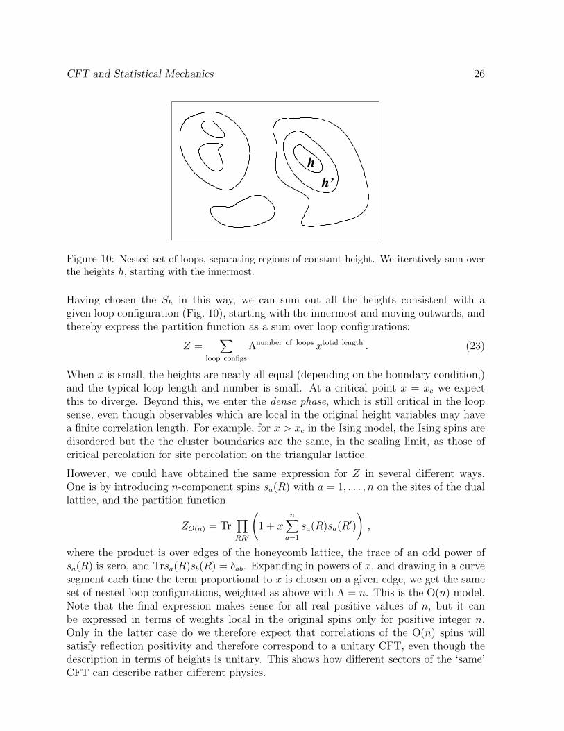
Figure 10: Nested set of loops, separating regions of constant height. We iteratively sum overthe heights h, starting with the innermost.

Having chosen the Sh in this way, we can sum out all the heights consistent with agiven loop configuration (Fig. 10), starting with the innermost and moving outwards, andthereby express the partition function as a sum over loop configurations:

Z =∑

loop configs

Λnumber of loops xtotal length . (23)

When x is small, the heights are nearly all equal (depending on the boundary condition,)and the typical loop length and number is small. At a critical point x = xc we expectthis to diverge. Beyond this, we enter the dense phase, which is still critical in the loopsense, even though observables which are local in the original height variables may havea finite correlation length. For example, for x > xc in the Ising model, the Ising spins aredisordered but the the cluster boundaries are the same, in the scaling limit, as those ofcritical percolation for site percolation on the triangular lattice.

However, we could have obtained the same expression for Z in several different ways.One is by introducing n-component spins sa(R) with a = 1, . . . , n on the sites of the duallattice, and the partition function

ZO(n) = Tr∏RR′

(1 + x

n∑a=1

sa(R)sa(R′)

),

where the product is over edges of the honeycomb lattice, the trace of an odd power ofsa(R) is zero, and Trsa(R)sb(R) = δab. Expanding in powers of x, and drawing in a curvesegment each time the term proportional to x is chosen on a given edge, we get the sameset of nested loop configurations, weighted as above with Λ = n. This is the O(n) model.Note that the final expression makes sense for all real positive values of n, but it canbe expressed in terms of weights local in the original spins only for positive integer n.Only in the latter case do we therefore expect that correlations of the O(n) spins willsatisfy reflection positivity and therefore correspond to a unitary CFT, even though thedescription in terms of heights is unitary. This shows how different sectors of the ‘same’CFT can describe rather different physics.


Figure 11: Non-contractible loops on the cylinder can be taken into account by the insertion ofa suitable factor along a seam.

6.2 Coulomb gas methods

These loop models can be solved in various ways, for example by realising that theirtransfer matrix gives a representation of the Temperley-Lieb algebra, but a more powerfulif less rigorous method is to use the so-called Coulomb gas approach. Recalling thearguments of the previous section, we see that yet another way of getting to (23) is bystarting from a different height model, where now the heights h(r) are defined on theintegers (times π, for historical reasons) πZ. As long as we choose the correct eigenvalueof the adjacency matrix, this will give the same loop gas weights. That is we take G tobe A∞. In this case the eigenvectors correspond to plane wave modes propagating alongthe graph, labelled by a quasi-momentum χ with |χ| < 1: Sh ∝ eiχh, whose eigenvalue isΛ = 2 cos(πχ). Because these modes are chiral, we have to orient the loops to distinguishbetween χ and −χ. Each oriented loop then gets weighted with a factor e±iπχ/6 at eachvertex of the honeycomb lattice it goes through, depending on whether it turns to the leftor the right.

This version of the model, where the heights are unbounded, is much easier to analyse,at least non-rigorously. In particular, we might expect that in the scaling limit, aftercoarse-graining, we can treat h(r) as taking all real values, and write down an effectivefield theory. This should have the property that it is local, invariant under h(r)→ h(r)+constant, and with no terms irrelevant under the RG (that is, entering the effective actionwith positive powers of a.) The only possibility is a free gaussian field theory, with action

S = (g0/4π)∫

(∇h)2d2r .

However, this cannot be the full answer, because we know this corresponds to a CFT withc = 1. The resolution of this is most easily understood by considering the theory on a longcylinder of length ` and circumference L � `. Non-contractible loops which go aroundthe cylinder have the same number of inside and outside corners, so they are incorrectlycounted. This can be corrected by inserting a factor

∏t eiχh(t,0)e−iχh(t+1,0), which counts

each loop passing between (t, 0) and (t + 1, 0) with just the right factors e±iπχ. Thesefactors accumulate to eiχh(−`/2,0)e−iχh(`/2,0), corresponding to charges ±χ at the ends ofthe cylinder. This means that the partition function is

Z ∼ Zc=1〈eiχh(`/2)e−iχh(−`/2)〉 .


But we know (Sec. 3.1) that this correlation function decays like r−2xχ in the plane, wherexq = q2/2g0, and therefore on the cylinder

Z ∼ eπ`/6L e−2π(χ2/2g0)`/L ,

from which we see that the central charge is actually

c = 1− 6χ2

g0

.

However, we haven’t yet determined g0. This is fixed by the requirement that the screeningfields e±i2h(r), which come from the the fact that originally h(r) ∈ πZ, should be marginal,that is they do not affect the scaling behaviour so that we can add them to the actionwith impunity. This requires that they have scaling dimension x2 = 2. However, now xqshould be calculated from the cylinder with the charges e±iχh(±`/2) at the ends:

xq =(q ± χ)2

g0

− χ2

g0

=q2 ± 2χq

g0

. (24)

Setting x2 = 2 we then find g0 = 1± χ and therefore

c = 1− 6(g0 − 1)2

g0

.

6.3 Identification with minimal models

The partition function for the height models (at least on cylinder) depends only on theeigenvalue Λ of the adjacency matrix and hence the Coulomb gas should work equallywell for the models on Am if we set χ = k/(m + 1). The corresponding central charge isthen

c = 1− 6k2

(m+ 1)(m+ 1± k).

If we compare this with the formula for the minimal models

c = 1− 6(p− p′)2

pp′,

we are tempted to identify k = p− p′ and m+ 1 = p′. This implies g0 = p/p′, which cantherefore be identified with the parameter g introduced in the Kac formula.21 Moreover,if we compute the scaling dimensions of local fields φr(R) = cos ((r − 1)kh(R)/(m + 1))using (24) we find perfect agreement with the leading diagonal ∆r,r of the Kac table.22

We therefore have strong circumstantial evidence that the scaling limit of the dilute Ap′−1

21The other solution corresponds to interchanging p′ and p.22These are the relevant fields in the RG sense.


models (choosing the eigenvalue Λ = 2 cos(π(p−p′)/p′)) is the (p, p′) minimal model withp > p′. Note that only if k = 1, that is p = p′ + 1, are these CFTs unitary, and this isprecisely the case where the weights of the lattice model are real and positive.

For other graphs G we can try to make a similar identification. However, this is goingto work only if the maximal eigenvalue of the adjacency matrix of G is strictly less than2. A famous classification then shows that this restricts G to be either of the form Am,Dm or one of three exceptional cases E6,7,8.23 These other graphs also have eigenvalues ofthe same form (refeigen) as Am, but with m+ 1 now being the Coxeter number, and theallowed integers k being only a subset of those appearing in the A-series. These correspondto the Kac labels of the allowed scalar operators which appear in the appropriate modularinvariant partition function.

7 Boundary conformal field theory

7.1 Conformal boundary conditions and Ward identities

So far we haven’t considered what happens at the boundary of the domain D. This is asubject with several important applications, for example to quantum impurity problems(see the lectures by Affleck) and to D-branes in string theory.

In any field theory in a domain with a boundary, one needs to consider how to imposea set of consistent boundary conditions. Since CFT is formulated independently of aparticular set of fundamental fields and a lagrangian, this must be done in a more generalmanner. A natural requirement is that the off-diagonal component T‖⊥ of the stresstensor parallel/perpendicular to the boundary should vanish. This is called the conformalboundary condition. If the boundary is parallel to the time axis, it implies that there isno momentum flow across the boundary. Moreover, it can be argued that, under the RG,any uniform boundary condition will flow into a conformally invariant one. For a givenbulk CFT, however, there may be many possible distinct such boundary conditions, andit is one task of BCFT to classify these.

To begin with, take the domain to be the upper half plane, so that the boundary is thereal axis. The conformal boundary condition then implies that T (z) = T (z) when z is onthe real axis. This has the immediate consequence that correlators of T are those of Tanalytically continued into the lower half plane. The conformal Ward identity now reads

〈T (z)∏j

φj(zj, zj)〉 =∑j

(∆j

(z − zj)2+

1

z − zj∂zj

23Λ = 2 corresponds to the extended diagrams Am, etc., which give interesting rational CFTs withc = 1. However models based on graphs with Λ > 2 probably have a different kind of a transition atwhich the mean loop length remains finite.


+∆j

(z − zj)2+

1

z − zj∂zj

)〈∏j

φj(zj, zj)〉 . (25)

In radial quantisation, in order that the Hilbert spaces defined on different hypersurfacesbe equivalent, one must now choose semicircles centered on some point on the boundary,conventionally the origin. The dilatation operator is now

D =1

2πi

∫Sz T (z)dz − 1

2πi

∫Sz T (z)dz , (26)

where S is a semicircle. Using the conformal boundary condition, this can also be writtenas

D = L0 =1

2πi

∫Cz T (z)dz , (27)

where C is a complete circle around the origin.

Note that there is now only one Virasoro algebra. This is related to the fact that con-formal mappings which preserve the real axis correspond to real analytic functions. Theeigenstates of L0 correspond to boundary operators φj(0) acting on the vacuum state |0〉.It is well known that in a renormalizable QFT fields at the boundary require a differentrenormalization from those in the bulk, and this will in general lead to a different set ofconformal weights. It is one of the tasks of BCFT to determine these, for a given allowedboundary condition.

However, there is one feature unique to boundary CFT in two dimensions. Radial quan-tization also makes sense, leading to the same form (27) for the dilation operator, if theboundary conditions on the negative and positive real axes are different. As far as thestructure of BCFT goes, correlation functions with this mixed boundary condition be-have as though a local scaling field were inserted at the origin. This has led to the term‘boundary condition changing (bcc) operator’.

7.2 CFT on the annulus and classification of boundary states

Just as consideration of the partition function on the torus illuminates the bulk operatorcontent n∆,∆, it turns out that consistency on the annulus helps classify both the allowedboundary conditions, and the boundary operator content. To this end, consider a CFTin an annulus formed of a rectangle of unit width and height δ, with the top and bottomedges identified (see Fig. 12). The boundary conditions on the left and right edges, labelledby a, b, . . ., may be different. The partition function with boundary conditions a and b oneither edge is denoted by Zab(δ).

One way to compute this is by first considering the CFT on an infinitely long strip of unitwidth. This is conformally related to the upper half plane (with an insertion of boundarycondition changing operators at 0 and ∞ if a 6= b) by the mapping z → (1/π) ln z. Thegenerator of infinitesimal translations along the strip is

Hab = πD − πc/24 = πL0 − c/24 . (28)


1

δba

Figure 12: The annulus, with boundary conditions a and b on either boundary.

Thus for the annulusZab(δ) = Tr e−δ Hab = Tr qL0−πc/24 , (29)

with q ≡ e−πδ. As before, this can be decomposed into characters

Zab(δ) =∑∆

n∆ab χ∆(q) , (30)

but note that now the expression is linear. The non-negative integers n∆ab give the operator

content with the boundary conditions (ab): the lowest value of ∆ with n∆ab > 0 gives the

conformal weight of the bcc operator, and the others give conformal weights of the otherallowed primary fields which may also sit at this point.

On the other hand, the annulus partition function may be viewed, up to an overall rescal-ing, as the path integral for a CFT on a circle of unit circumference, being propagatedfor (imaginary) time δ−1. From this point of view, the partition function is no longer a

trace, but rather the matrix element of e−H/δ between boundary states:

Zab(δ) = 〈a|e−H/δ|b〉 . (31)

Note that H is the same hamiltonian that appears on the cylinder, and the boundarystates lie in the Hilbert space of states on the circle. They can be decomposed into linearcombinations of states in the representation spaces of the two Virasoro algebras, labelledby their lowest weights (∆,∆).

How are these boundary states to be characterized? Recalling that on the cylinder Ln ∝∫einuT (u)du, and Ln ∝

∫e−inuT (u)du, the conformal boundary condition implies that

any boundary state |B〉 lies in the subspace satisfying

Ln|B〉 = L−n|B〉 . (32)


This condition can be applied in each subspace. Taking n = 0 in (32) constrains ∆ = ∆.It can then be shown that the solution of (32) is unique within each subspace and has thefollowing form. The subspace at level N of has dimension d∆(N). Denote an orthonormalbasis by |∆, N ; j〉, with 1 ≤ j ≤ d∆(N), and the same basis for the representation spaceof Vir by |∆, N ; j〉. The solution to (32) in this subspace is then

|∆〉〉 ≡∞∑N=0

d∆(N)∑j=1

|∆, N ; j〉 ⊗ |∆, N ; j〉 . (33)

These are called Ishibashi states. One way to understand this is to note that (32) impliesthat

〈B|Ln|B〉 = 〈B|L−n|B〉 = 〈B|Ln|B〉 ,

where we have used L†−n = Ln and assumed that the matrix elements are all real. This

means that acting with the raising operators Ln on |B〉 has exactly the same effect as theLn, so, starting with N = 0 we must build up exactly the same state in the two spaces.

Matrix elements of the translation operator along the cylinder between Ishibashi statesare simple:

〈〈∆′|e−H/δ|∆〉〉 (34)

=∞∑

N ′=0

d∆′ (N ′)∑j′=1

∞∑N=0

d∆(N)∑j=1

〈∆′, N ′; j′| ⊗ 〈∆′, N ′; j′|e−(2π/δ)(L0+ˆL0−c/12)

|∆, N ; j〉 ⊗ |∆, N ; j〉 (35)

= δ∆′∆

∞∑N=0

d∆(N)∑j=1

e−(4π/δ)(∆+N−(c/24)) = δ∆′∆ χ∆(e−4π/δ) . (36)

Note that the characters which appear are related to those in (30) by the modular trans-formation S.

The physical boundary states satisfying (30) are linear combinations of these Ishibashistates:

|a〉 =∑∆

〈〈∆|a〉 |∆〉〉 . (37)

Equating the two different expressions (30,31) for Zab, and using the modular trans-formation law for the characters and their linear independence, gives the (equivalent)conditions:

n∆ab =

∑∆′S∆

∆′〈a|∆′〉〉〈〈∆′|b〉 ; (38)

〈a|∆′〉〉〈〈∆′|b〉 =∑∆

S∆′

∆ n∆ab . (39)

The requirements that the right hand side of (38) should give a non-negative integer,and that the right hand side of (39) should factorize in a and b, give highly nontrivialconstraints on the allowed boundary states and their operator content.


∆∆

0

0 ∆

∆

Figure 13: Argument illustrating the fusion rules.

For the diagonal CFTs considered here (and for the nondiagonal minimal models) acomplete solution is possible. Since the elements S∆

0 of S are all non-negative, one may

choose 〈〈∆|0〉 = (S∆0 )1/2. This defines a boundary state

|0〉 ≡∑∆

(S∆0 )1/2|∆〉〉 , (40)

and a corresponding boundary condition such that n∆00 = δ∆0. Then, for each ∆′ 6= 0, one

may define a boundary state

〈〈∆|∆′〉 ≡ S∆∆′/(S∆

0 )1/2 . (41)

From (38), this gives n∆∆′0 = δ∆′∆. For each allowed ∆′ in the torus partition function,

there is therefore a boundary state |∆′〉 satisfying (38,39). However, there is a furtherrequirement:

n∆∆′∆′′ =

∑`

S∆` S

`∆′S`∆′′

S`0(42)

should be a non-negative integer. Remarkably, this combination of elements of S occursin the Verlinde formula, which follows from considering consistency of the CFT on thetorus. This states that the right hand side of (42) is equal to the fusion rule coefficientN∆

∆′∆′′ . Since these are non-negative integers, the above ansatz for the boundary states isconsistent. The appearance of the fusion rules in this context can be understood by thefollowing argument, illustrated in Fig. 13. Consider a very long strip. At ‘time’ t→ −∞the boundary conditions on both sides are those corresponding to 0, so that only statesin the representation 0 propagate. At time t1 we insert the bcc operator (0|∆′) on oneedge: the states ∆′ then propagate. This can be thought of as the fusion of 0 with ∆′.At some much later time we insert the bcc operator (0|∆′′) on the other edge: by thesame argument this should correspond to the fusion of ∆′ and ∆′′, which gives all states∆ with N∆

∆′,∆′′ = 1. But by definition, these are those with n∆∆′,∆′′ = 1.

We conclude that, at least for the diagonal models, there is a bijection between theallowed primary fields in the bulk CFT and the allowed conformally invariant boundaryconditions. For the minimal models, with a finite number of such primary fields, thiscorrespondence has been followed through explicitly.


7.2.1 Example

The simplest example is the diagonal c = 12

unitary CFT corresponding to p = 4, p′ = 3.The allowed values of the conformal weights are h = 0, 1

2116

, and

S =

12

12

1√2

12

12

− 1√2

1√2− 1√

20

, (43)

from which one finds the allowed boundary states

|0〉 = 1√2|0〉〉+ 1√

2|12〉〉+ 1

21/4 | 116〉〉 ; (44)

| 12〉 = 1√

2|0〉〉+ 1√

2|12〉〉 − 1

21/4 | 116〉〉 ; (45)

| 116〉 = |0〉〉 − |1

2〉〉 . (46)

The nonzero fusion rule coefficients of this CFT are

N00,0 = N

116

0, 116

= N12

0, 12

= N0116, 116

= N12116, 116

= N012, 12

= N116116, 12

= 1 .

The c = 12

CFT is known to describe the continuum limit of the critical Ising model, inwhich spins s = ±1 are localized on the sites of a regular lattice. The above boundaryconditions may be interpreted as the continuum limit of the lattice boundary conditionss = 1, s = −1 and free (f), respectively. Note there is a symmetry of the fusion rules whichmeans that one could equally well have reversed the first two. This shows, for example,that the for (ff) boundary conditions the states with lowest weights 0 (correspondingto the identity operator) and 1

2(corresponding to the the magnetisation operator at the

boundary) can propagate. Similarly, the scaling dimension of the (f | ± 1) bcc operator is116

.

7.3 Boundary operators and SLE

Let us now apply the above ideas to the Am models. There should be a set of conformalboundary states corresponding to the entries of first row (r, 1) of the Kac table, with1 ≤ r ≤ m. It is an educated guess (confirmed by exact calculations) that these in factcorrespond to lattice boundary conditions where the heights on the boundary are fixed tobe at a particular node r of the Am graph. What about the boundary condition changingoperators? These are given by the fusion rules. In particular, since (suppressing the indexs = 1)

N r′

r,2 = δ|r−r′|,1 ,

we see that the bcc operator between r and r ± 1, corresponding to a single clusterboundary intersecting the boundary of the domain, must be a (2, 1) operator in the Kac


table.24 This makes complete sense: if we want to go from r1 to r2 we must bring togetherat least |r1−r2| cluster boundaries, showing that the leading bcc operator in this case is at(|r1−r2|, 1), consistent once again with the fusion rules. If the bcc operators correspondingto a single curve are (2, 1) this means that the corresponding states satisfy

(2L−2 − (2/g)L2−1)|φ2,1〉 = 0 . (47)

We are now going to argue that (47) is equivalent to the statement that the clusterboundary starting at this boundary point is described by SLE. In order to avoid beingtoo abstract initially, we’ll first show how the calculations of a particular observable agreein the two different formalisms.

Let ζ be a point in the upper half plane and let P (ζ) be the probability that the curve,starting at the origin, passes to the left of this point (of course it is not holomorphic).First we’ll give the physicist’s version of the SLE argument (assuming familiarity withWerner’s lectures). We imagine making the exploration process for a small Loewner timeδt, then continuing the process to infinity. Under the conformal mapping fδt(z) whichremoves the first part of the curve, we get a new curve with the same measure as theoriginal one, but the point ζ is mapped to fδt(ζ). But this will lie to the right of thenew curve if and only if the original point lay to the right of the original curve. Also, byintegrating the Loewner equation starting from f0(z) = z, we have approximately

fδt(z) ≈ z +2δt

z+√κδBt ,

at least for z � δt. Thus we can write down an equation25:

P (ζ) = E

[P

(ζ +

2δt

ζ+√κδBt

)]δBt

,

where E[. . .]δBt means an average over all realisations of the Brownian motion up to timeδt. Expanding the right hand side to O(δt), and remembering that E[δBt] = 0 andE[(δBt)

2] = δt, we find (with ζ = x+ iy), the linear PDE(2x

x2 + y2

∂

∂x− 2y

x2 + y2

∂

∂y+κ

2

∂2

∂x2

)P (x, y) = 0 . (48)

By scale invariance, P (x, y) depends in fact only on the ratio y/x, and therefore this canbe reduced to a second order ODE, whose solution, with appropriate boundary condi-tions, can be expressed in terms of hypergeometric functions (and is known as Schramm’sformula.)

24If instead of the dilute lattice model we consider the dense phase, which corresponds, eg to theboundaries of the FK clusters in the Potts model, then r and s get interchanged for a given centralcharge c, and the bcc operator then lies at (1, 2).

25Some physicists will recognise this as the reverse Fokker-Planck equation.


Now let us give the CFT derivation. In terms of correlation functions, P can be expressedas

P =〈φ2,1(0)Φ(ζ, ζ)φ2,1(∞)〉〈φ2,1(0)φ2,1(∞)〉

.

The denominator is just the partition function restricted to there being a cluster boundaryfrom 0 to infinity. Φ is an ‘indicator operator’ which takes the values 0 or 1 dependingon whether the curve passes to the right (respectively left) of ζ. Since P is a probabilityit is dimensionless, so Φ has zero conformal dimensions and transforms trivially.

Now suppose we insert∫C(2T (z)/z)(dz/2πi) + cc. into the correlation function in the

numerator, where C is a semicircular contour surrounding the origin but not ζ. Using theOPE of T with φ2,1, this gives

2L−2φ2,1(0) = (2/g)∂2xφ1,2(x)|x=0 .

Using translation invariance, this derivative can be made to act equivalently on the x-coordinate of ζ. On the other hand, we can also distort the contour to wrap around ζ,where it simply shifts the argument of Φ. The result is that we get exactly the same PDEas in (48), with the identification

g = 4/κ .

Of course this was just one example. Let us see how to proceed more generally. Inradial quantisation, the insertion of the bcc field φ2,1(0) gives a state |φ2,1〉. Under theinfinitesimal mapping fdt we get the state(

1− (2L−2dt+ L−1

√κdBt)

)|φ2,1〉 ,

or, over a finite time, a time-ordered exponential

T exp(−∫ t

0(L−2dt

′ + L−1

√κdBt′)

)|φ2,1〉 . (49)

The conformal invariance property of the measure on the curve then implies that, whenaveraged over dBt′ , this is in fact independent of t. Expanding to O(t) we then againfind (47) with g = 4/κ. Since this is a property of the state, it implies an equivalencebetween the two approaches for all correlation functions involving φ2,1(0), not just the oneconsidered earlier. Moreover if we replace

√κdBt by some more general random driving

function dWt, and expand (49) to any finite order in t using the Virasoro algebra andthe null state condition, we can determine all moments of Wt and conclude that it mustindeed be rescaled Brownian motion.

Of course the steps we used to arrive at this result in CFT are far less rigorous than themethods of SLE. However, CFT is more powerful in the sense that many other similarresult can be conjectured which, at present, seem to be beyond the techniques of SLE.This is part of an ongoing symbiosis between the disciplines of theoretical physics andmathematics which, one hopes, will continue.


8 Further Reading

The basic reference for CFT is the ‘big yellow book’: Conformal Field Theory by P. diFrancesco, P. Mathieu and D. Senechal (Springer-Verlag, 1996.) See also volume 2 ofStatistical Field Theory by C. Itzykson and J.-M. Drouffe (Cambridge University Press,1989.) A gentler introduction is provided in the 1988 les Houches lectures by P. Ginspargand J. Cardy in Fields, Strings and Critical Phenomena, E. Brezin and J. Zinn-Justin,eds. (North-Holland, 1990.) Other specific pedagogical references are given below.

2.1 J. Cardy, Scaling and Renormalization in Statistical Physics, (Cambridge UniversityPress, 1996.)

3.2 P. Calabrese and J. Cardy, Entanglement entropy and quantum field theory – a non-technical introduction, Int.J.Quant.Inf. 4, 429 (2006); arXiv:quant-ph/0505193.

6.1 V. Pasquier, Nucl. Phys. B 285, 162, 1986, and J. Phys. A 20, L1229, 1987;I. Kostov, Nucl. Phys. B 376, 539, 1992; arXiv:hep-th/9112059. The version inthese lectures is discussed in J. Cardy, J.Phys. A 40, 1427 (2007); arXiv:math-ph/0610030.

6.2 The basic reference is B. Nienhuis, in Phase transitions and critical phenomena,vol. 11, p. 1, C. Domb and J.L. Lebowitz, eds. (Academic, 1987.) A slightlydifferent approach is explained in J. Kondev, Phys. Rev. Lett. 78, 4320, 1997.

7.1,7.2 For reviews see V.B. Petkova and J.-B. Zuber, Conformal boundary conditions andwhat they teach us, lectures given at the Summer School and Conference on Non-perturbative Quantum Field Theoretic Methods and their Applications, August2000, Budapest, Hungary, arXiv:hep-th/0103007, and J. Cardy, Boundary Con-formal Field Theory in Encyclopedia of Mathematical Physics, (Elsevier, 2006);arXiv:hep-th/0411189.

7.3 For reviews on the connection between SLE and CFT, see J. Cardy, SLE for The-oretical Physicists, Ann. Phys. 318, 81-118 (2005); arXiv:cond-mat/0503313,and M. Bauer and D. Bernard, 2D growth processes: SLE and Loewner chains,Phys.Rept. 432, 115-221 (2006); arXiv:math-ph/0602049.

Conformal Field Theory and Statistical Mechanics · Conformal Field Theory and Statistical...

Documents

Transcript of Conformal Field Theory and Statistical Mechanics · Conformal Field Theory and Statistical...