Confirmatory factor analysis in - restore.ac.uk · Confirmatory factor analysis in ... Analysing...

Confirmatory factor analysis in

Mplus

Day 2

1

Agenda 1. EFA and CFA common rules and best practice

Model identification considerations

Choice of rotation

Checking the standard errors (ensuring identification)

Checking fit and the residuals

2. Analysing test scales (Thurstone’s mental abilities example)

3. Analysing item-level test data A. Single dimension

Binary / Ordinal responses

B. Multiple dimensions (Big Five questionnaire example)

4. Some common problems with fitting common factor models to item-level data

A. Negatively keyed items

Modelling acquiescence bias (Random intercept model, Bifactor model)

Repeated content and correlated errors

Cross-loadings

2

Common rules and best practice

Multiple-factor model

3

Conducting EFA in practice

Model identification considerations

Choice of rotation

Checking the standard errors (ensuring identification)

Checking the fit and the residuals

Main reference: McDonald, R. (1999). Test Theory. Lawrence

Erlbaum.

4

Independent clusters

Item or test that indicates only 1 factor is called

factorially simple

Item or test that indicates 2 or more factor is called

factorially complex

Independent clusters factor model – every variable is an

indicator for only 1 factor (every variable is factorially

simple)

5

Identification 1

Exploratory model (unrestricted common factor model)

In single-factor case, the loadings and unique variances are

determined by the covariances and variances of original

variables (the model is identified)

In the more general case of 2 or more factors, the system of

equations describing the variables through common factors

does not have a unique solution

There are infinite number of models that fit the data equally well

Further constraints are required

Fortunately, they often correspond to the test design

6

Identification 2

Two forms of lack of identifiability

1. Exchange of factor loadings while unique variances are identified and unchanging (rotation problem)

Resolved by assigning arbitrary loadings and then transforming them into an approximation to an independent clusters pattern

2. Joint indeterminacy of factor loadings and unique variances – hidden doublet factors

1. Happens because for just two tests, 12=12 cannot be solved uniquely for 1 and 2

2. In EFA with uncorrelated factors this cannot be resolved and is hidden by the analysis

3. Subtle but worrying problem

7

Identification 3

General conditions for identification

1. For each factor, there are at least 3 indicators with non-

zero loadings that have 0 loadings on all other factors

(each factor has at least 3 factorially simple indicators)

2. For each factor, there are at least 2 indicators with non-

zero loadings that have 0 loadings on all other factors,

and also, any factor that have 2 defining indicators is

correlated with other factors

There are important for CFA, but are also useful to diagnose

problems with EFA

8

Rotation 1

Rotation is a transformation of parameters to

approximate an independent cluster solution

Factors are uncorrelated (orthogonal rotation) or

correlated (oblique rotation)

McDonald (Test Theory, 1999) shows convincingly why

oblique rotations are to be preferred

They avoid identification problems which will create “doublets”

factors

For most applications correlated factors are more conceptually

sound

Even if factors are found to be uncorrelated in one population,

they might be correlated in another

9

Rotation 2

Many rotation algorithms are available in Mplus

For orthogonal rotations

There are just rotated loadings to interpret

For oblique rotations

There is a pattern matrix (like coefficients in multiple

regression - correlations between indicators and the factor

with other indicators partialled out)

There is also a structure matrix (correlations between

indicators and the factor)

Correlations between the factors

10

Checking the standard errors

For an identified model, SE should be approximately equal

If so, it is safe to proceed with the exploratory analysis

If not, it might indicate an indeterminacy with doublet

factors

1/ n

11

Practical 1 – continuous data

Analysing test scale data

12

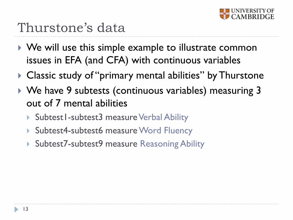
Thurstone’s data

We will use this simple example to illustrate common

issues in EFA (and CFA) with continuous variables

Classic study of “primary mental abilities” by Thurstone

We have 9 subtests (continuous variables) measuring 3

out of 7 mental abilities

Subtest1-subtest3 measure Verbal Ability

Subtest4-subtest6 measure Word Fluency

Subtest7-subtest9 measure Reasoning Ability

13

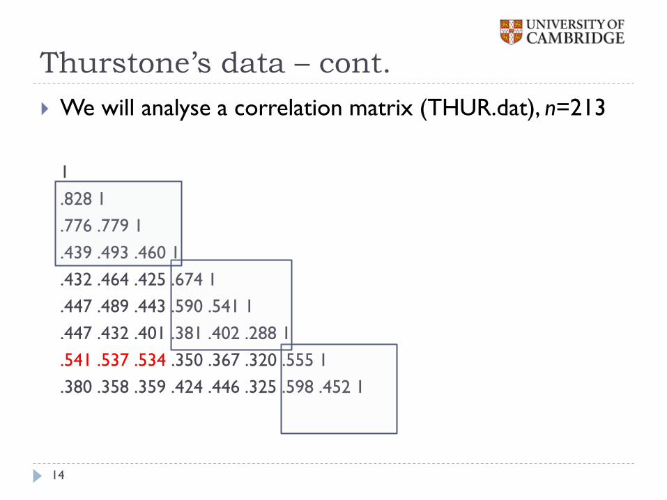
We will analyse a correlation matrix (THUR.dat), n=213

1

.828 1

.776 .779 1

.439 .493 .460 1

.432 .464 .425 .674 1

.447 .489 .443 .590 .541 1

.447 .432 .401 .381 .402 .288 1

.541 .537 .534 .350 .367 .320 .555 1

.380 .358 .359 .424 .446 .325 .598 .452 1

Thurstone’s data – cont.

14

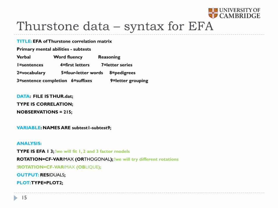
Thurstone data – syntax for EFA TITLE: EFA of Thurstone correlation matrix

Primary mental abilities - subtests

Verbal Word fluency Reasoning

1=sentences 4=first letters 7=letter series

2=vocabulary 5=four-letter words 8=pedigrees

3=sentence completion 6=suffixes 9=letter grouping

DATA: FILE IS THUR.dat;

TYPE IS CORRELATION;

NOBSERVATIONS = 215;

VARIABLE: NAMES ARE subtest1-subtest9;

ANALYSIS:

TYPE IS EFA 1 3; !we will fit 1, 2 and 3 factor models

ROTATION=CF-VARIMAX (ORTHOGONAL); !we will try different rotations

!ROTATION=CF-VARIMAX (OBLIQUE);

OUTPUT: RESIDUALS;

PLOT: TYPE=PLOT2;

15

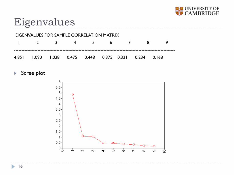
Eigenvalues EIGENVALUES FOR SAMPLE CORRELATION MATRIX

1 2 3 4 5 6 7 8 9

--------------------------------------------------------------------------------------------------------------

4.851 1.090 1.038 0.475 0.448 0.375 0.321 0.234 0.168

Scree plot

16

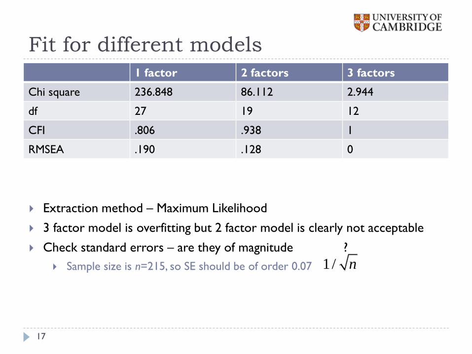
Fit for different models

1 factor 2 factors 3 factors

Chi square 236.848 86.112 2.944

df 27 19 12

CFI .806 .938 1

RMSEA .190 .128 0

Extraction method – Maximum Likelihood

3 factor model is overfitting but 2 factor model is clearly not acceptable

Check standard errors – are they of magnitude ?

Sample size is n=215, so SE should be of order 0.07

1/ n

17

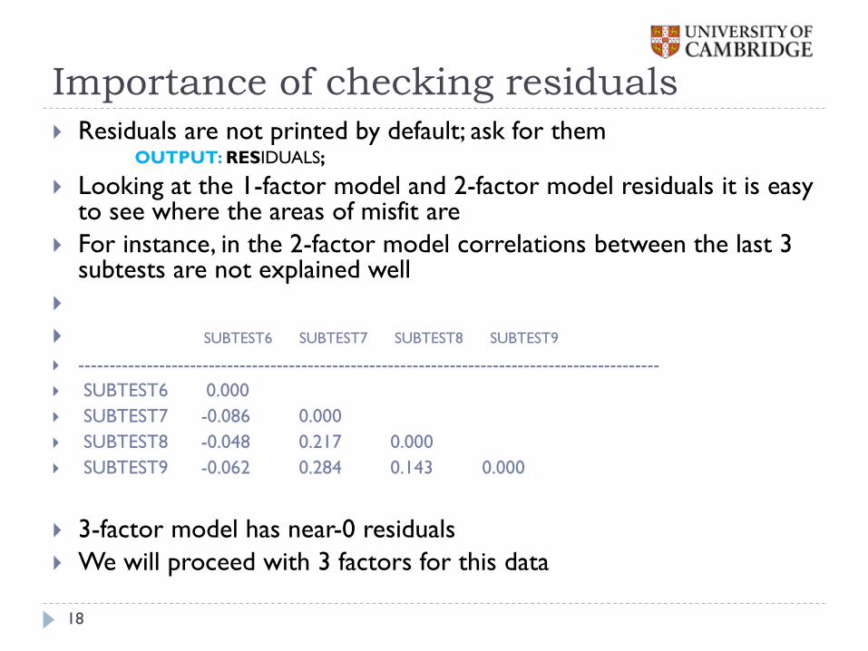
Importance of checking residuals Residuals are not printed by default; ask for them

OUTPUT: RESIDUALS;

Looking at the 1-factor model and 2-factor model residuals it is easy to see where the areas of misfit are

For instance, in the 2-factor model correlations between the last 3 subtests are not explained well

SUBTEST6 SUBTEST7 SUBTEST8 SUBTEST9

----------------------------------------------------------------------------------------------

SUBTEST6 0.000

SUBTEST7 -0.086 0.000

SUBTEST8 -0.048 0.217 0.000

SUBTEST9 -0.062 0.284 0.143 0.000

3-factor model has near-0 residuals

We will proceed with 3 factors for this data

18

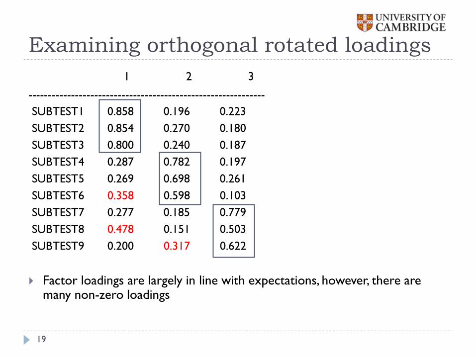
Examining orthogonal rotated loadings

1 2 3

-------------------------------------------------------------

SUBTEST1 0.858 0.196 0.223

SUBTEST2 0.854 0.270 0.180

SUBTEST3 0.800 0.240 0.187

SUBTEST4 0.287 0.782 0.197

SUBTEST5 0.269 0.698 0.261

SUBTEST6 0.358 0.598 0.103

SUBTEST7 0.277 0.185 0.779

SUBTEST8 0.478 0.151 0.503

SUBTEST9 0.200 0.317 0.622

Factor loadings are largely in line with expectations, however, there are many non-zero loadings

19

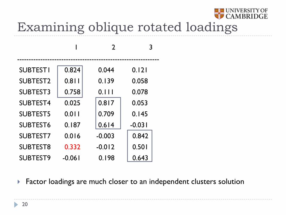
Examining oblique rotated loadings

1 2 3

-------------------------------------------------------------

SUBTEST1 0.824 0.044 0.121

SUBTEST2 0.811 0.139 0.058

SUBTEST3 0.758 0.111 0.078

SUBTEST4 0.025 0.817 0.053

SUBTEST5 0.011 0.709 0.145

SUBTEST6 0.187 0.614 -0.031

SUBTEST7 0.016 -0.003 0.842

SUBTEST8 0.332 -0.012 0.501

SUBTEST9 -0.061 0.198 0.643

Factor loadings are much closer to an independent clusters solution

20

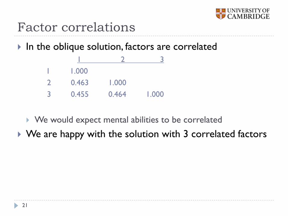
Factor correlations

In the oblique solution, factors are correlated

1 2 3

1 1.000

2 0.463 1.000

3 0.455 0.464 1.000

We would expect mental abilities to be correlated

We are happy with the solution with 3 correlated factors

21

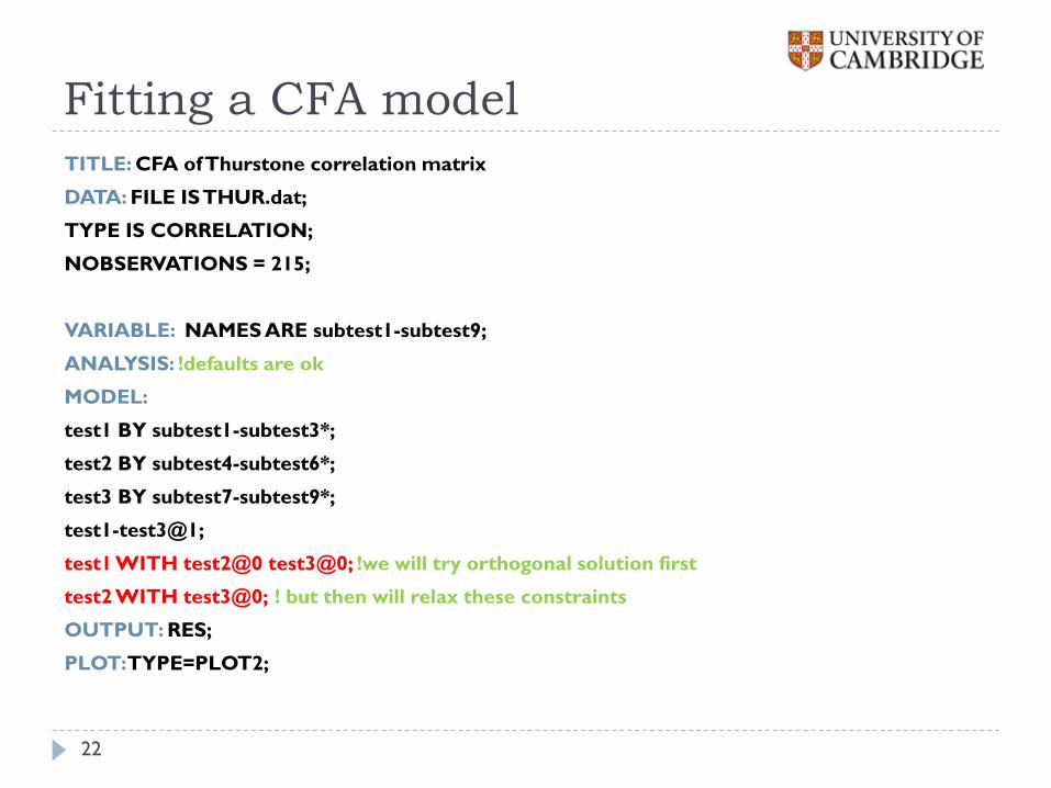
Fitting a CFA model

TITLE: CFA of Thurstone correlation matrix

DATA: FILE IS THUR.dat;

TYPE IS CORRELATION;

NOBSERVATIONS = 215;

VARIABLE: NAMES ARE subtest1-subtest9;

ANALYSIS: !defaults are ok

MODEL:

test1 BY subtest1-subtest3*;



test1-test3@1;

test1 WITH test2@0 test3@0; !we will try orthogonal solution first

test2 WITH test3@0; ! but then will relax these constraints

OUTPUT: RES;

PLOT: TYPE=PLOT2;

22

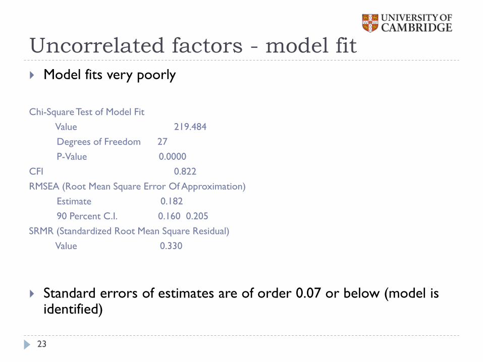
Uncorrelated factors - model fit

Model fits very poorly

Chi-Square Test of Model Fit

Value 219.484

Degrees of Freedom 27

P-Value 0.0000

CFI 0.822

RMSEA (Root Mean Square Error Of Approximation)

Estimate 0.182

90 Percent C.I. 0.160 0.205

SRMR (Standardized Root Mean Square Residual)

Value 0.330

Standard errors of estimates are of order 0.07 or below (model is identified)

23

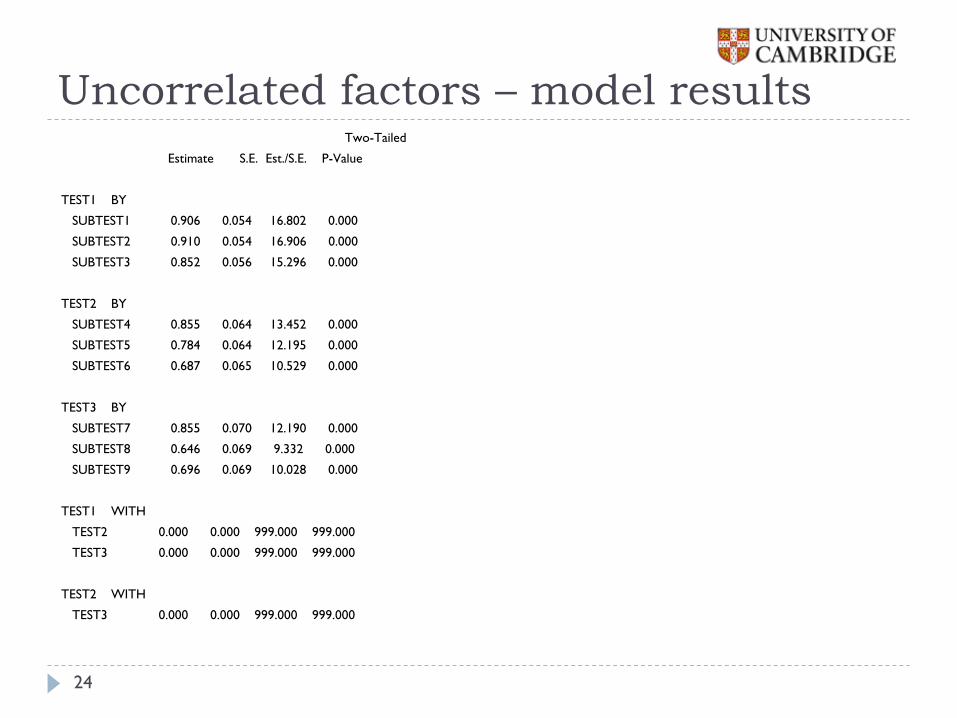
Uncorrelated factors – model results Two-Tailed

Estimate S.E. Est./S.E. P-Value

TEST1 BY

SUBTEST1 0.906 0.054 16.802 0.000

SUBTEST2 0.910 0.054 16.906 0.000

SUBTEST3 0.852 0.056 15.296 0.000

TEST2 BY

SUBTEST4 0.855 0.064 13.452 0.000

SUBTEST5 0.784 0.064 12.195 0.000

SUBTEST6 0.687 0.065 10.529 0.000

TEST3 BY

SUBTEST7 0.855 0.070 12.190 0.000

SUBTEST8 0.646 0.069 9.332 0.000

SUBTEST9 0.696 0.069 10.028 0.000

TEST1 WITH

TEST2 0.000 0.000 999.000 999.000

TEST3 0.000 0.000 999.000 999.000

TEST2 WITH

TEST3 0.000 0.000 999.000 999.000

24

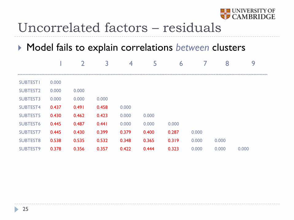
Uncorrelated factors – residuals

Model fails to explain correlations between clusters

1 2 3 4 5 6 7 8 9

--------------------------------------------------------------------------------------------------------------------------------------------------------------

SUBTEST1 0.000

SUBTEST2 0.000 0.000

SUBTEST3 0.000 0.000 0.000

SUBTEST4 0.437 0.491 0.458 0.000

SUBTEST5 0.430 0.462 0.423 0.000 0.000

SUBTEST6 0.445 0.487 0.441 0.000 0.000 0.000

SUBTEST7 0.445 0.430 0.399 0.379 0.400 0.287 0.000

SUBTEST8 0.538 0.535 0.532 0.348 0.365 0.319 0.000 0.000

SUBTEST9 0.378 0.356 0.357 0.422 0.444 0.323 0.000 0.000 0.000

25

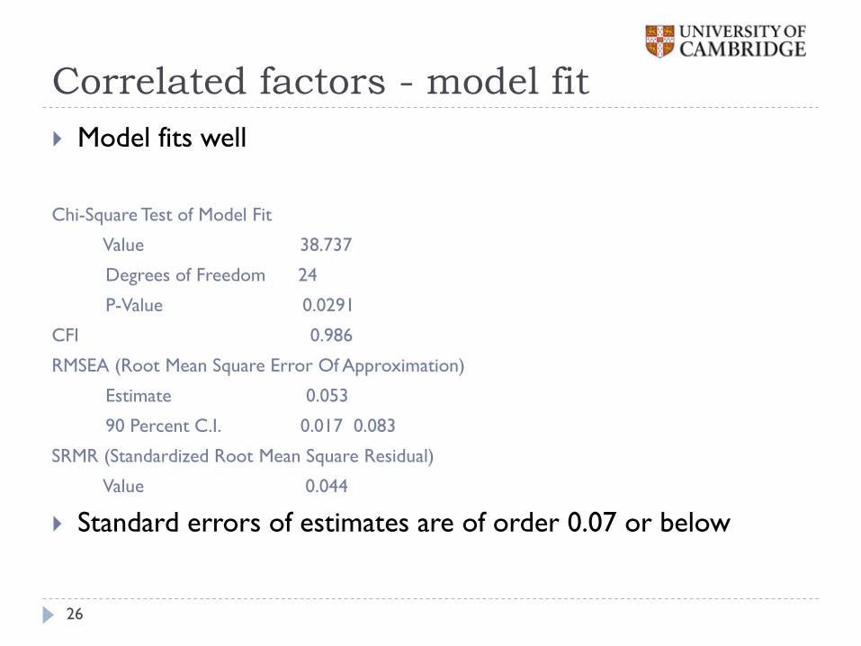
Correlated factors - model fit

Model fits well

Chi-Square Test of Model Fit

Value 38.737


P-Value 0.0291

CFI 0.986

RMSEA (Root Mean Square Error Of Approximation)

Estimate 0.053

90 Percent C.I. 0.017 0.083

SRMR (Standardized Root Mean Square Residual)

Value 0.044

Standard errors of estimates are of order 0.07 or below

26

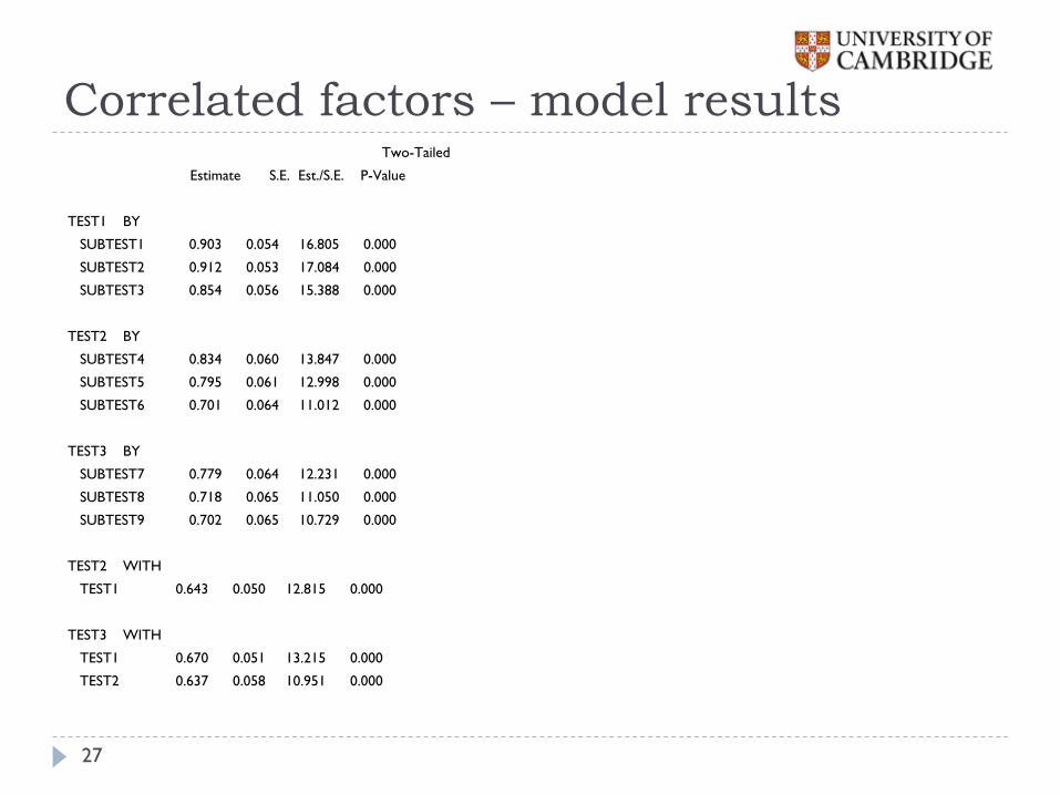
Correlated factors – model results Two-Tailed


TEST1 BY

SUBTEST1 0.903 0.054 16.805 0.000

SUBTEST2 0.912 0.053 17.084 0.000

SUBTEST3 0.854 0.056 15.388 0.000

TEST2 BY

SUBTEST4 0.834 0.060 13.847 0.000

SUBTEST5 0.795 0.061 12.998 0.000

SUBTEST6 0.701 0.064 11.012 0.000

TEST3 BY

SUBTEST7 0.779 0.064 12.231 0.000

SUBTEST8 0.718 0.065 11.050 0.000

SUBTEST9 0.702 0.065 10.729 0.000

TEST2 WITH

TEST1 0.643 0.050 12.815 0.000

TEST3 WITH

TEST1 0.670 0.051 13.215 0.000

TEST2 0.637 0.058 10.951 0.000

27

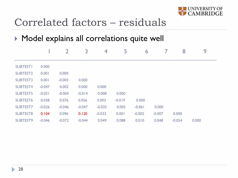
Correlated factors – residuals

Model explains all correlations quite well

1 2 3 4 5 6 7 8 9

--------------------------------------------------------------------------------------------------------------------------------------------------------------

SUBTEST1 0.000

SUBTEST2 0.001 0.000

SUBTEST3 0.001 -0.003 0.000

SUBTEST4 -0.047 0.002 0.000 0.000

SUBTEST5 -0.031 -0.004 -0.014 0.008 0.000

SUBTEST6 0.038 0.076 0.056 0.003 -0.019 0.000

SUBTEST7 -0.026 -0.046 -0.047 -0.035 0.005 -0.061 0.000

SUBTEST8 0.104 0.096 0.120 -0.033 0.001 -0.002 -0.007 0.000

SUBTEST9 -0.046 -0.072 -0.044 0.049 0.088 0.010 0.048 -0.054 0.000

28

Analysing item-level test data

Categorical data considerations

29

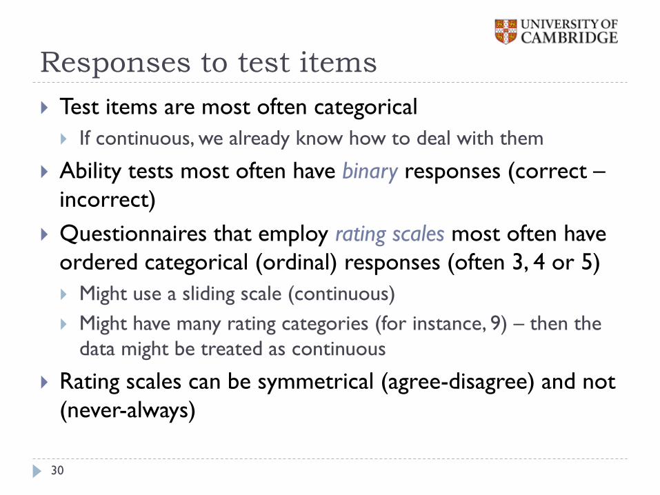
Responses to test items

Test items are most often categorical

If continuous, we already know how to deal with them

Ability tests most often have binary responses (correct –

incorrect)

Questionnaires that employ rating scales most often have

ordered categorical (ordinal) responses (often 3, 4 or 5)

Might use a sliding scale (continuous)

Might have many rating categories (for instance, 9) – then the

data might be treated as continuous

Rating scales can be symmetrical (agree-disagree) and not

(never-always)

30

Correlations between items

31

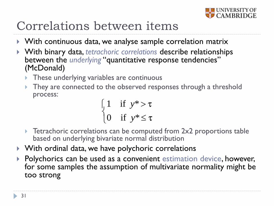
With continuous data, we analyse sample correlation matrix

With binary data, tetrachoric correlations describe relationships between the underlying “quantitative response tendencies” (McDonald) These underlying variables are continuous

They are connected to the observed responses through a threshold process:

Tetrachoric correlations can be computed from 2x2 proportions table based on underlying bivariate normal distribution

With ordinal data, we have polychoric correlations

Polychorics can be used as a convenient estimation device, however, for some samples the assumption of multivariate normality might be too strong

1 if *

0 if *

y

y

Item factor analysis

32

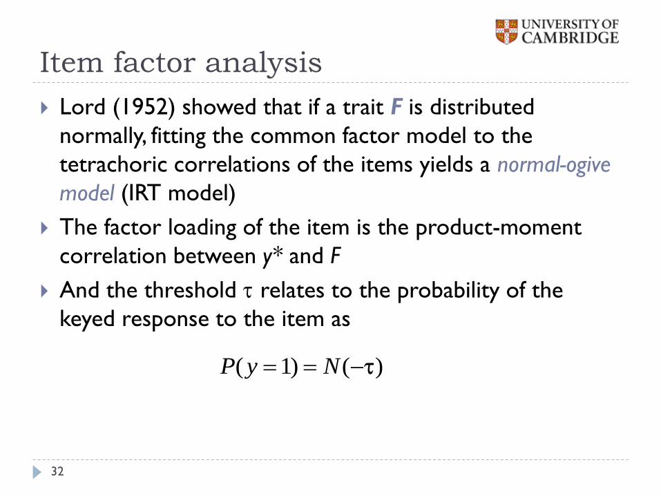
Lord (1952) showed that if a trait F is distributed

normally, fitting the common factor model to the

tetrachoric correlations of the items yields a normal-ogive

model (IRT model)

The factor loading of the item is the product-moment

correlation between y* and F

And the threshold relates to the probability of the

keyed response to the item as

( 1) ( )P y N

Practical 2 – binary data


33

Inductive reasoning test

34

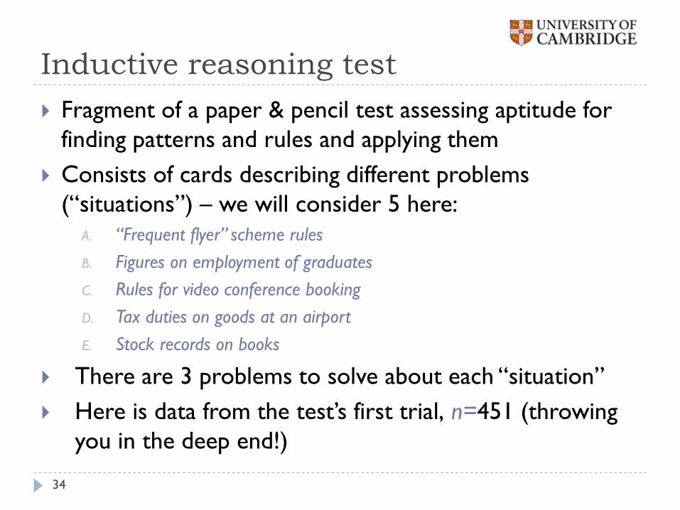
Fragment of a paper & pencil test assessing aptitude for

finding patterns and rules and applying them

Consists of cards describing different problems

(“situations”) – we will consider 5 here:

A. “Frequent flyer” scheme rules

B. Figures on employment of graduates

C. Rules for video conference booking

D. Tax duties on goods at an airport

E. Stock records on books

There are 3 problems to solve about each “situation”

Here is data from the test’s first trial, n=451 (throwing

you in the deep end!)

EFA

35

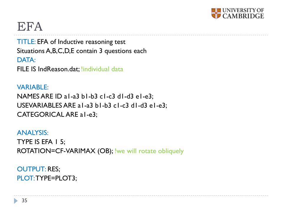
TITLE: EFA of Inductive reasoning test

Situations A,B,C,D,E contain 3 questions each

DATA:

FILE IS IndReason.dat; !individual data

VARIABLE:

NAMES ARE ID a1-a3 b1-b3 c1-c3 d1-d3 e1-e3;

USEVARIABLES ARE a1-a3 b1-b3 c1-c3 d1-d3 e1-e3;

CATEGORICAL ARE a1-e3;

ANALYSIS:

TYPE IS EFA 1 5;

ROTATION=CF-VARIMAX (OB); !we will rotate obliquely

OUTPUT: RES;

PLOT: TYPE=PLOT3;

How many factors?

36

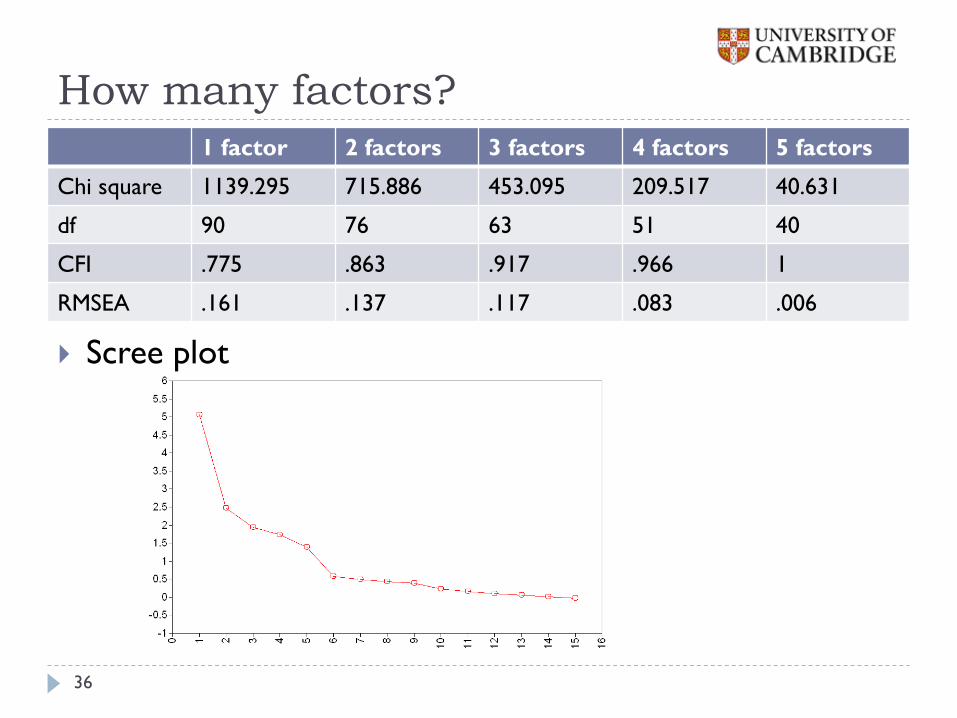
Scree plot

1 factor 2 factors 3 factors 4 factors 5 factors

Chi square 1139.295 715.886 453.095 209.517 40.631

df 90 76 63 51 40

CFI .775 .863 .917 .966 1

RMSEA .161 .137 .117 .083 .006

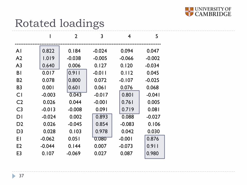
Rotated loadings

37

1 2 3 4 5

-----------------------------------------------------------------------------------

A1 0.822 0.184 -0.024 0.094 0.047

A2 1.019 -0.038 -0.005 -0.066 -0.002

A3 0.640 0.006 0.127 0.120 -0.034

B1 0.017 0.911 -0.011 0.112 0.045

B2 0.078 0.800 0.072 -0.107 -0.025

B3 0.001 0.601 0.061 0.076 0.068

C1 -0.003 0.043 -0.017 0.801 -0.041

C2 0.026 0.044 -0.001 0.761 0.005

C3 -0.013 -0.008 0.091 0.719 0.081

D1 -0.024 0.002 0.893 0.088 -0.027

D2 0.026 -0.045 0.854 -0.083 0.106

D3 0.028 0.103 0.978 0.042 0.030

E1 -0.062 0.051 0.080 -0.001 0.876

E2 -0.044 0.144 0.007 -0.073 0.911

E3 0.107 -0.069 0.027 0.087 0.980

EFA model summary

38

Standard errors are around 0.05 as they should be; residuals are very small

Are there really 5 factors? Dooes each “situation” requires a distinct fundamental ability to read and interpret it?

Or, questions within each “situation” share common variance – method variance

If the examinee understood the “situation”, all questions relating to it are more likely to be answered correctly (and vice versa)

This leads to local dependencies of items within “situations” (correlated uniquenesses):

Common variance in the questions is explained by the overall factor, and unique variance in the questions is uncorrelated across “situations”, but is correlated within “situations”

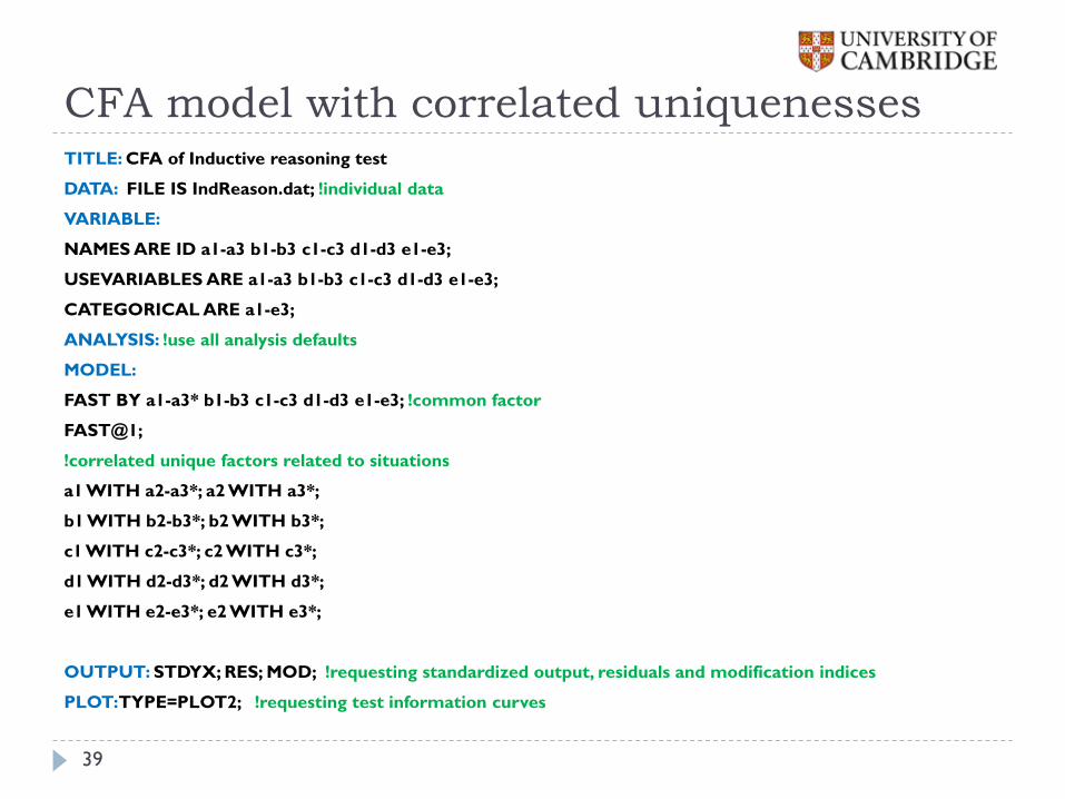
CFA model with correlated uniquenesses

39

TITLE: CFA of Inductive reasoning test

DATA: FILE IS IndReason.dat; !individual data

VARIABLE:

NAMES ARE ID a1-a3 b1-b3 c1-c3 d1-d3 e1-e3;

USEVARIABLES ARE a1-a3 b1-b3 c1-c3 d1-d3 e1-e3;

CATEGORICAL ARE a1-e3;

ANALYSIS: !use all analysis defaults

MODEL:

FAST BY a1-a3* b1-b3 c1-c3 d1-d3 e1-e3; !common factor

FAST@1;

!correlated unique factors related to situations

a1 WITH a2-a3*; a2 WITH a3*;

b1 WITH b2-b3*; b2 WITH b3*;

c1 WITH c2-c3*; c2 WITH c3*;

d1 WITH d2-d3*; d2 WITH d3*;

e1 WITH e2-e3*; e2 WITH e3*;

OUTPUT: STDYX; RES; MOD; !requesting standardized output, residuals and modification indices

PLOT: TYPE=PLOT2; !requesting test information curves

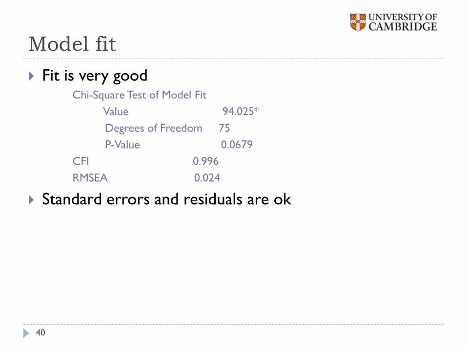
Model fit

40

Fit is very good Chi-Square Test of Model Fit

Value 94.025*


P-Value 0.0679

CFI 0.996

RMSEA 0.024

Standard errors and residuals are ok

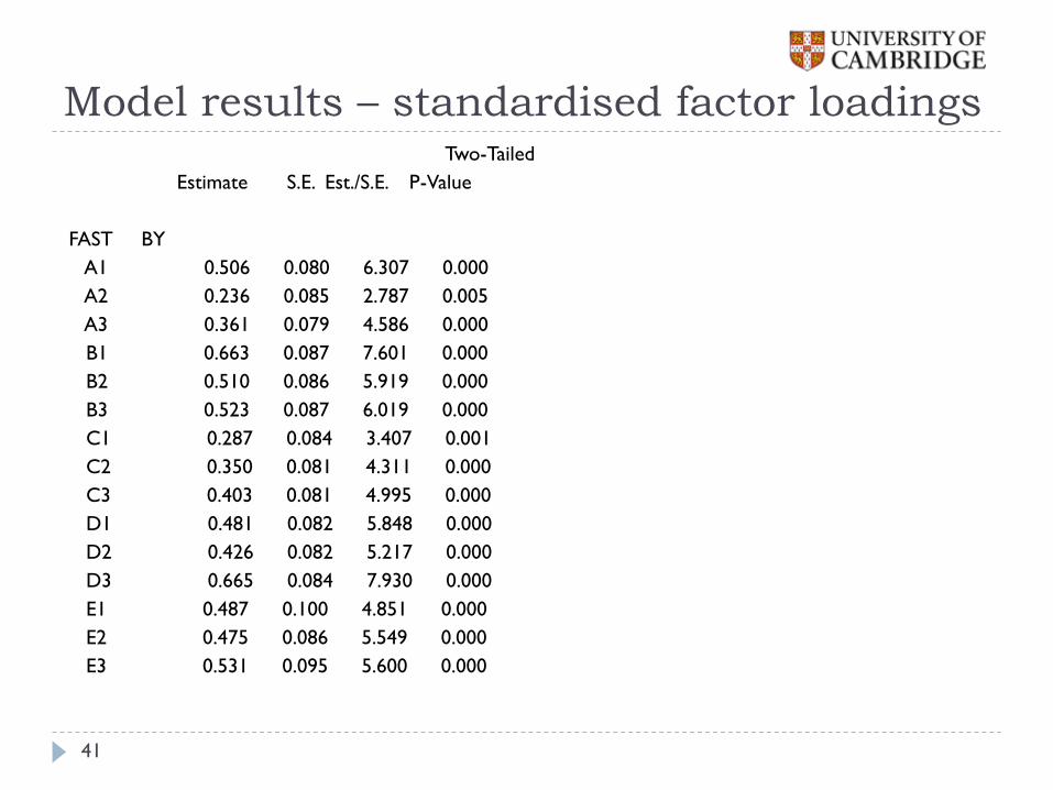
Model results – standardised factor loadings

41

Two-Tailed


FAST BY

A1 0.506 0.080 6.307 0.000

A2 0.236 0.085 2.787 0.005

A3 0.361 0.079 4.586 0.000

B1 0.663 0.087 7.601 0.000

B2 0.510 0.086 5.919 0.000

B3 0.523 0.087 6.019 0.000

C1 0.287 0.084 3.407 0.001

C2 0.350 0.081 4.311 0.000

C3 0.403 0.081 4.995 0.000

D1 0.481 0.082 5.848 0.000

D2 0.426 0.082 5.217 0.000

D3 0.665 0.084 7.930 0.000

E1 0.487 0.100 4.851 0.000

E2 0.475 0.086 5.549 0.000

E3 0.531 0.095 5.600 0.000

Correlated uniquenesses

42

Normal output will give covariances between residuals This is useful for evaluating how much residual variance is shared

between items from the same “situation”

To evaluate correlations between residuals, one has to examine STDYX output

Let’s take item B1 (look in your output) Factor loading .663 (R-square is .439, which means 43.9% of variance is

explained by the common “problem solving” factor)

Remaining residual variance is .561; out of which .415 is shared with B2, and .293 is shared with B3. So the “situation” explains roughly as much variance as the common factor.

Problem with correlated errors is that they violate the assumption of local independence

Estimation of trait scores and test information rests on this assumption

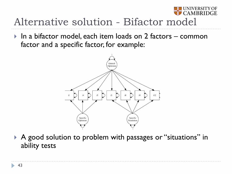
Alternative solution - Bifactor model

43

In a bifactor model, each item loads on 2 factors – common factor and a specific factor, for example:

A good solution to problem with passages or “situations” in ability tests

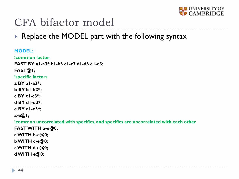
CFA bifactor model

44

Replace the MODEL part with the following syntax

MODEL:

!common factor

FAST BY a1-a3* b1-b3 c1-c3 d1-d3 e1-e3;

FAST@1;

!specific factors

a BY a1-a3*;

b BY b1-b3*;

c BY c1-c3*;

d BY d1-d3*;

e BY e1-e3*;

a-e@1;

!common uncorrelated with specifics, and specifics are uncorrelated with each other

FAST WITH a-e@0;

a WITH b-e@0;

b WITH c-e@0;

c WITH d-e@0;

d WITH e@0;

Bifactor model - results

45

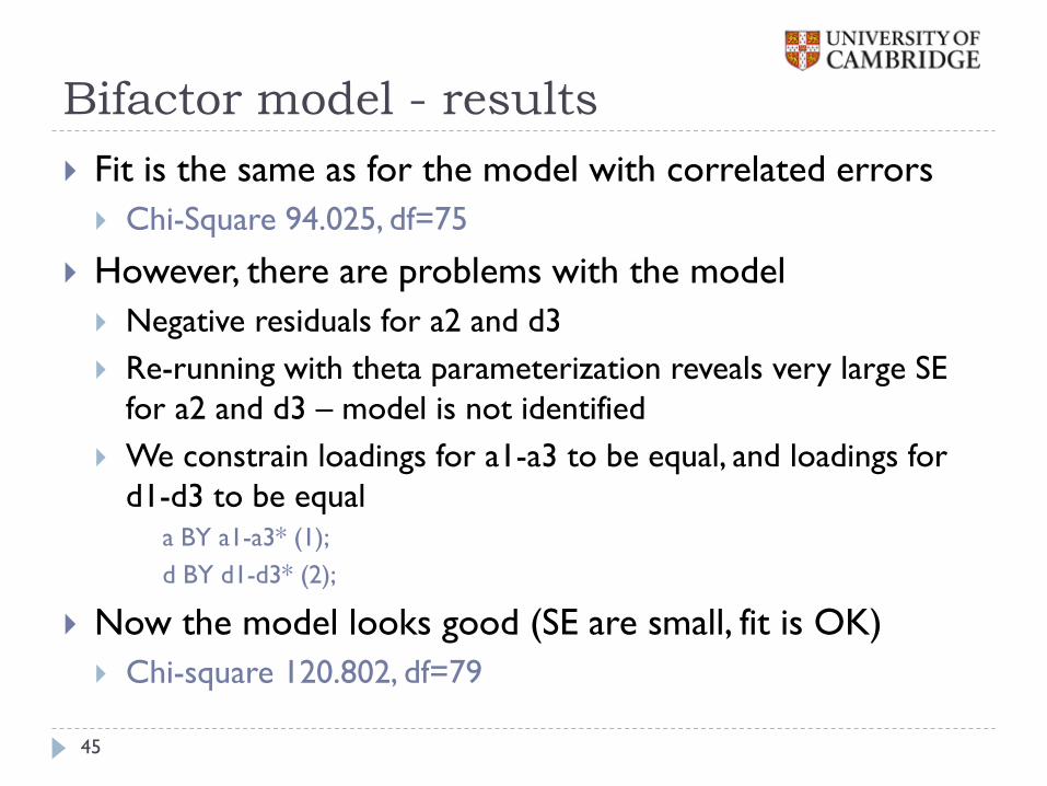
Fit is the same as for the model with correlated errors

Chi-Square 94.025, df=75

However, there are problems with the model

Negative residuals for a2 and d3

Re-running with theta parameterization reveals very large SE

for a2 and d3 – model is not identified

We constrain loadings for a1-a3 to be equal, and loadings for

d1-d3 to be equal

a BY a1-a3* (1);

d BY d1-d3* (2);

Now the model looks good (SE are small, fit is OK)

Chi-square 120.802, df=79

Practical 3 – ordinal data


46

Big Five questionnaire

47

Big Five personality factors (Goldberg, 1992)

Extraversion (or Surgency), Agreeableness, Emotional stability, Conscientiousness and Intellect (or Imagination)

IPIP (International Personality Item Pool), 100-item questionnaire measuring the Big Five

20 items per trait

5 symmetrical rating options:

Very Inaccurate / Moderately Inaccurate / Neither Accurate Nor Inaccurate / Moderately Accurate / Very Accurate

Coded 1,2,3,4,5 (ordinal scale)

Volunteer sample, N=319

Goldberg, L. R. (1992). The development of markers for the Big-Five factor

structure. Psychological Assessment, 4, 26-42.

Extraversion

48

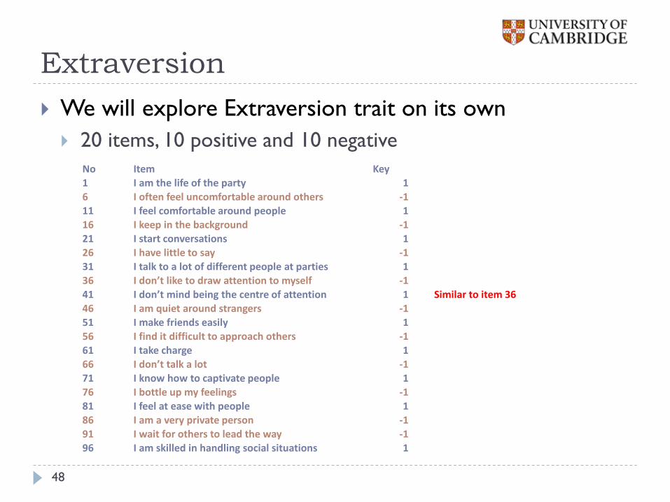
We will explore Extraversion trait on its own

20 items, 10 positive and 10 negative

No Item Key

1 I am the life of the party 1 6 I often feel uncomfortable around others -1 11 I feel comfortable around people 1 16 I keep in the background -1 21 I start conversations 1 26 I have little to say -1 31 I talk to a lot of different people at parties 1 36 I don’t like to draw attention to myself -1

41 I don’t mind being the centre of attention 1 Similar to item 36 46 I am quiet around strangers -1 51 I make friends easily 1 56 I find it difficult to approach others -1 61 I take charge 1 66 I don’t talk a lot -1 71 I know how to captivate people 1 76 I bottle up my feelings -1

81 I feel at ease with people 1 86 I am a very private person -1 91 I wait for others to lead the way -1 96 I am skilled in handling social situations 1

EFA - Extraversion

49

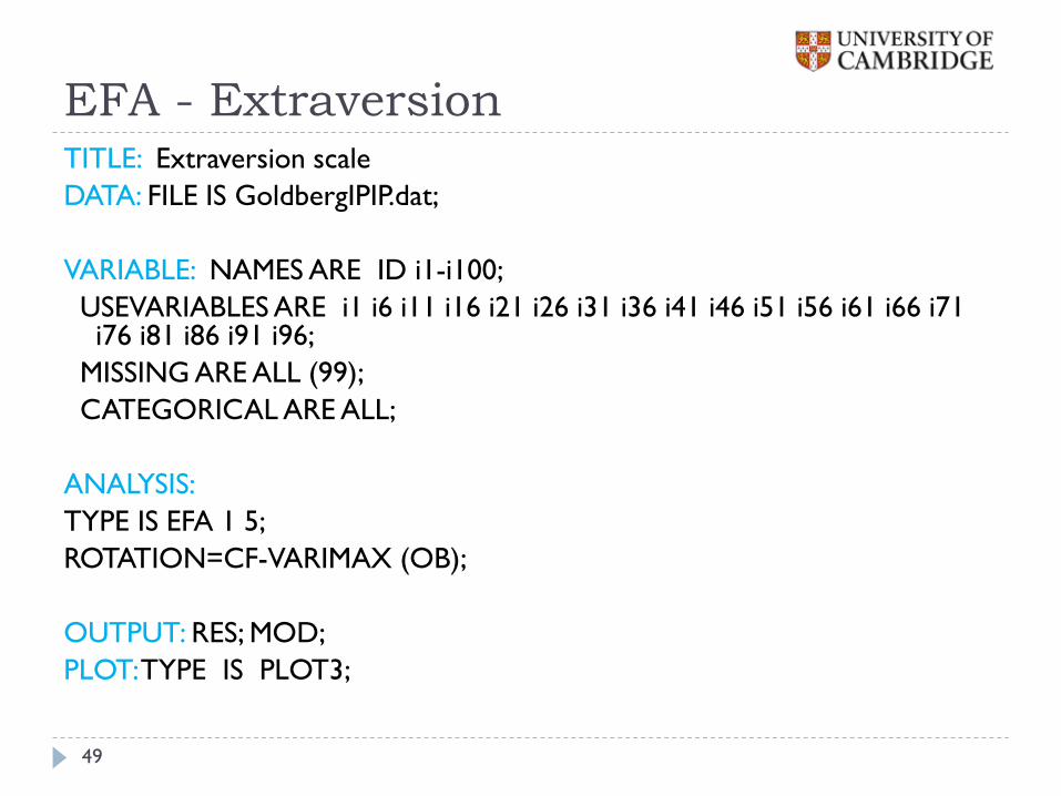
TITLE: Extraversion scale

DATA: FILE IS GoldbergIPIP.dat;

VARIABLE: NAMES ARE ID i1-i100;

USEVARIABLES ARE i1 i6 i11 i16 i21 i26 i31 i36 i41 i46 i51 i56 i61 i66 i71 i76 i81 i86 i91 i96;

MISSING ARE ALL (99);

CATEGORICAL ARE ALL;

ANALYSIS:

TYPE IS EFA 1 5;

ROTATION=CF-VARIMAX (OB);

OUTPUT: RES; MOD;

PLOT: TYPE IS PLOT3;

Extraversion - model fit

50

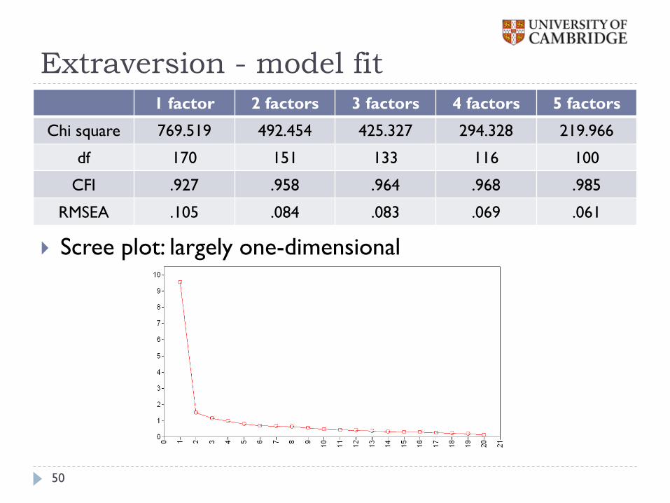
Model fit

Scree plot: largely one-dimensional


Chi square 769.519 492.454 425.327 294.328 219.966

df 170 151 133 116 100

CFI .927 .958 .964 .968 .985

RMSEA .105 .084 .083 .069 .061

One-dimensional?

51

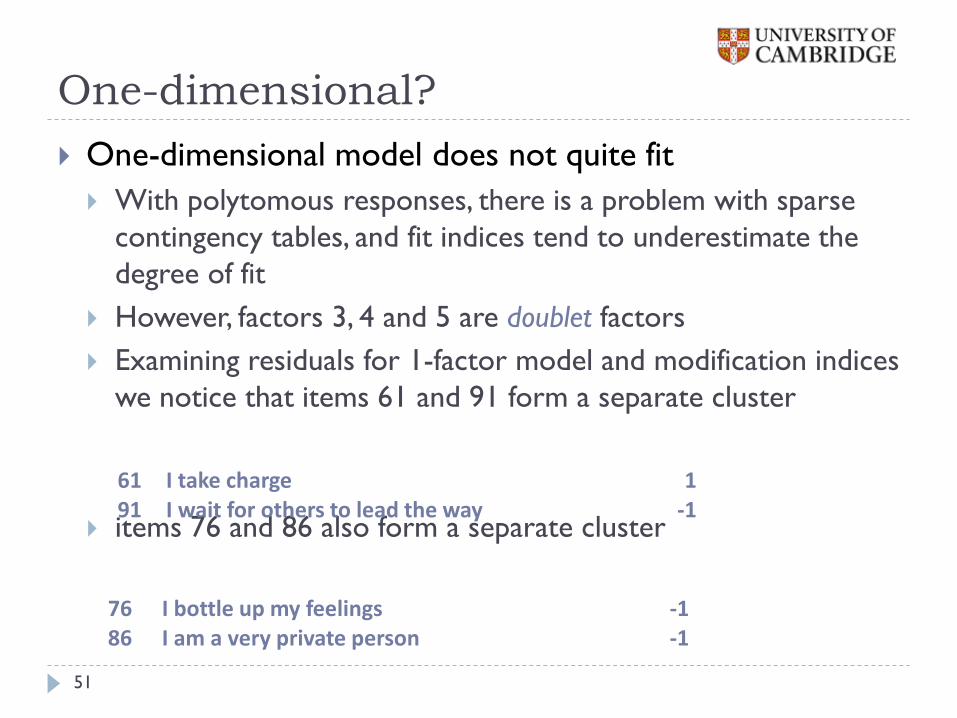
One-dimensional model does not quite fit

With polytomous responses, there is a problem with sparse

contingency tables, and fit indices tend to underestimate the

degree of fit

However, factors 3, 4 and 5 are doublet factors

Examining residuals for 1-factor model and modification indices

we notice that items 61 and 91 form a separate cluster

items 76 and 86 also form a separate cluster

61 I take charge 1 91 I wait for others to lead the way -1

76 I bottle up my feelings -1 86 I am a very private person -1

Improving the scale

52

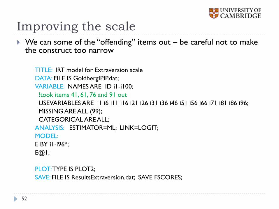
We can some of the “offending” items out – be careful not to make the construct too narrow

TITLE: IRT model for Extraversion scale



!took items 41, 61, 76 and 91 out

USEVARIABLES ARE i1 i6 i11 i16 i21 i26 i31 i36 i46 i51 i56 i66 i71 i81 i86 i96;



ANALYSIS: ESTIMATOR=ML; LINK=LOGIT;

MODEL:

E BY i1-i96*;

E@1;


SAVE: FILE IS ResultsExtraversion.dat; SAVE FSCORES;

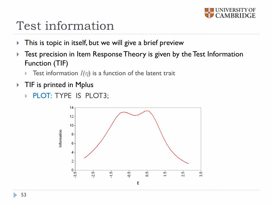
This is topic in itself, but we will give a brief preview

Test precision in Item Response Theory is given by the Test Information

Function (TIF)

Test information () is a function of the latent trait

TIF is printed in Mplus


Test information

53

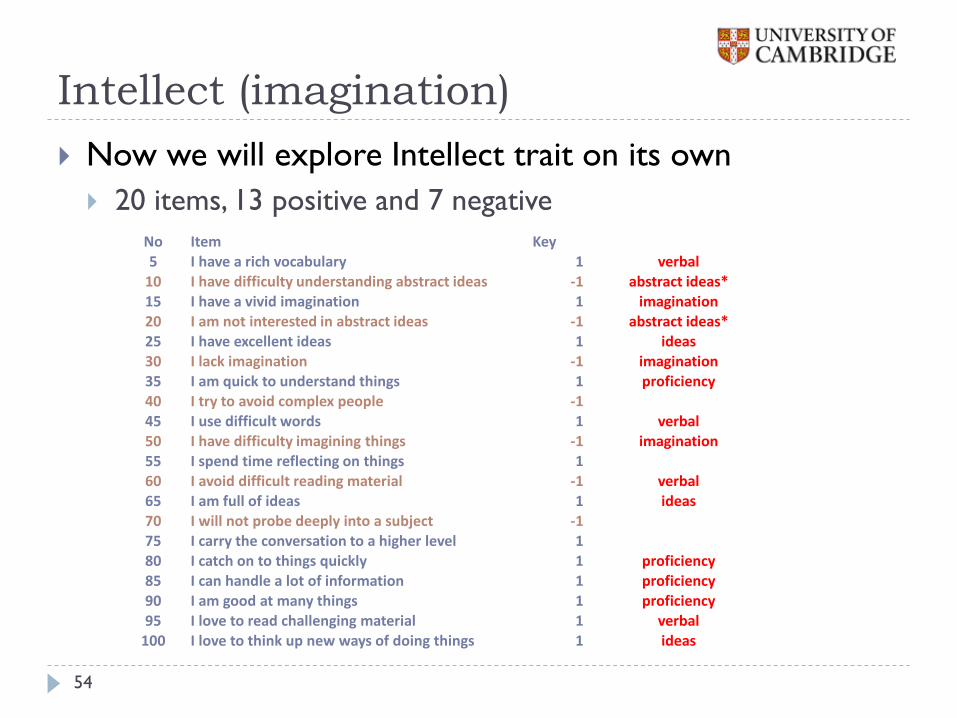
Intellect (imagination)

54

Now we will explore Intellect trait on its own

20 items, 13 positive and 7 negative

No Item Key

5 I have a rich vocabulary 1 verbal 10 I have difficulty understanding abstract ideas -1 abstract ideas* 15 I have a vivid imagination 1 imagination 20 I am not interested in abstract ideas -1 abstract ideas* 25 I have excellent ideas 1 ideas 30 I lack imagination -1 imagination 35 I am quick to understand things 1 proficiency 40 I try to avoid complex people -1

45 I use difficult words 1 verbal 50 I have difficulty imagining things -1 imagination 55 I spend time reflecting on things 1 60 I avoid difficult reading material -1 verbal 65 I am full of ideas 1 ideas 70 I will not probe deeply into a subject -1 75 I carry the conversation to a higher level 1 80 I catch on to things quickly 1 proficiency

85 I can handle a lot of information 1 proficiency 90 I am good at many things 1 proficiency 95 I love to read challenging material 1 verbal

100 I love to think up new ways of doing things 1 ideas

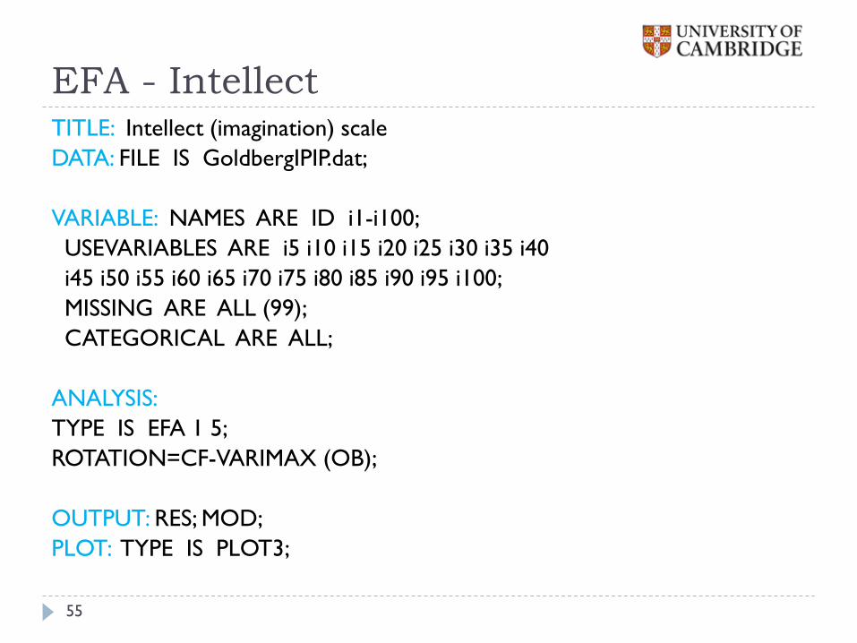
EFA - Intellect

55

TITLE: Intellect (imagination) scale



USEVARIABLES ARE i5 i10 i15 i20 i25 i30 i35 i40

i45 i50 i55 i60 i65 i70 i75 i80 i85 i90 i95 i100;



ANALYSIS:

TYPE IS EFA 1 5;


OUTPUT: RES; MOD;


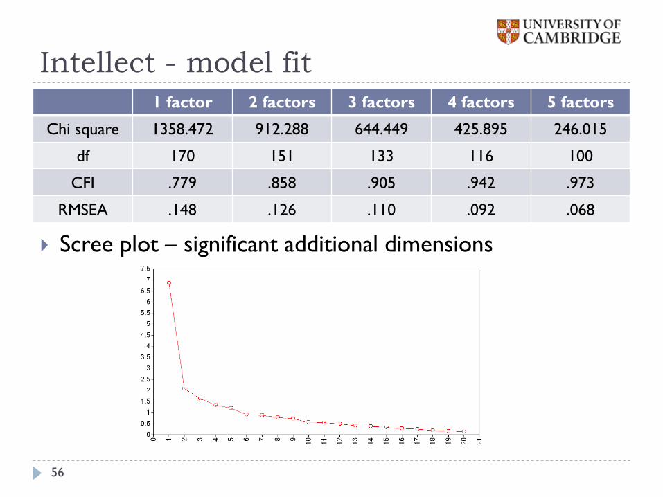
Intellect - model fit

56

Model fit

Scree plot – significant additional dimensions


Chi square 1358.472 912.288 644.449 425.895 246.015

df 170 151 133 116 100

CFI .779 .858 .905 .942 .973

RMSEA .148 .126 .110 .092 .068

How many factors?

57

One-dimensional model does not fit at all

There are meaningful sub-dimensions (see slide 53)

Verbal ability

Imagination

Fluency of ideas

Proficiency

There are also items that do not belong to any sub-dimension

However, in 5-factor solution, factor 1 is a doublet factor (items about “abstract ideas”)

Probably, 4 sub-dimensions exist within this set of items

Developer has several options – reduce dimensionality by taking some items out, or accommodate multi-dimensionality by fitting bifactor or higher-order models

Practical 4 – multidimensional

ordinal data


58

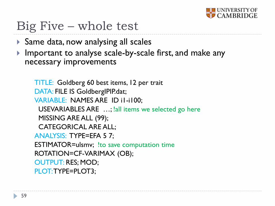
Big Five – whole test

59

Same data, now analysing all scales

Important to analyse scale-by-scale first, and make any necessary improvements

TITLE: Goldberg 60 best items, 12 per trait



USEVARIABLES ARE …; !all items we selected go here



ANALYSIS: TYPE=EFA 5 7;

ESTIMATOR=ulsmv; !to save computation time


OUTPUT: RES; MOD;

PLOT: TYPE=PLOT3;

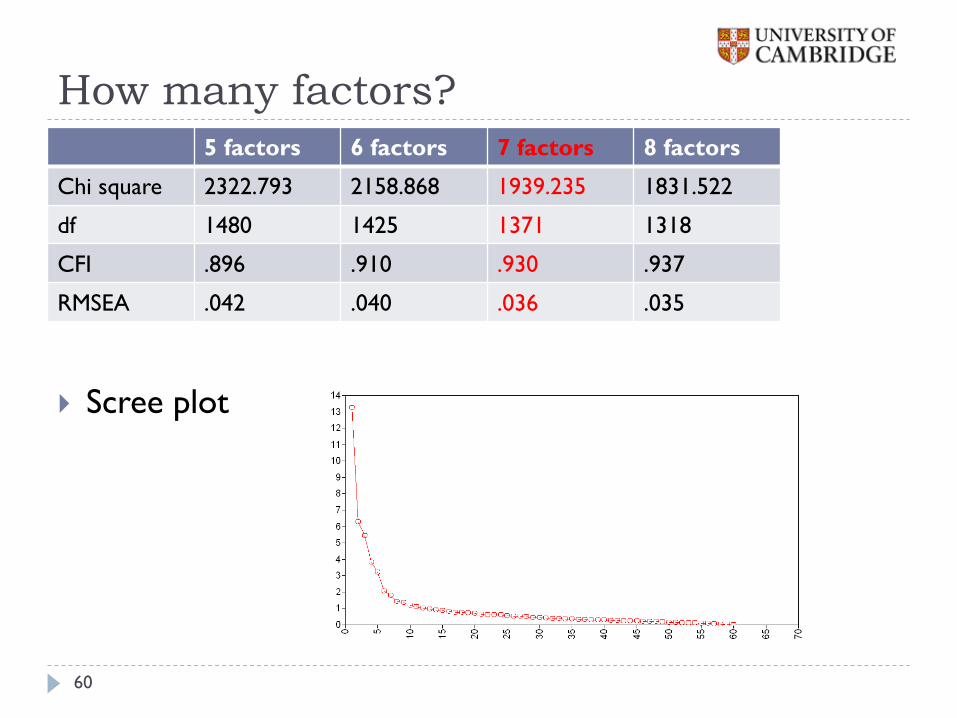
How many factors?

60

Scree plot

5 factors 6 factors 7 factors 8 factors

Chi square 2322.793 2158.868 1939.235 1831.522

df 1480 1425 1371 1318

CFI .896 .910 .930 .937

RMSEA .042 .040 .036 .035

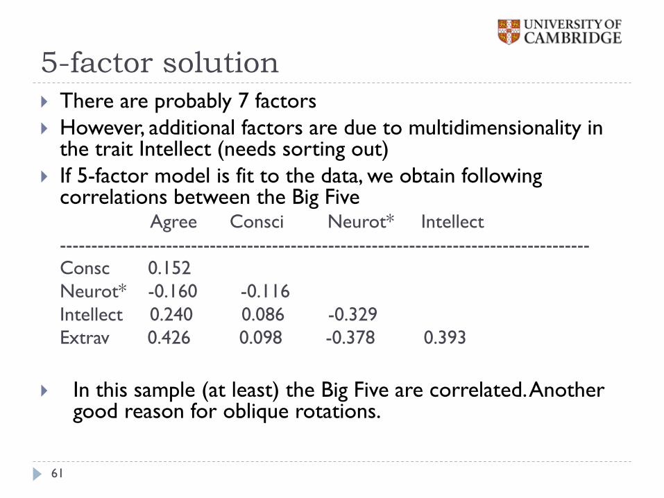
5-factor solution

61

There are probably 7 factors

However, additional factors are due to multidimensionality in the trait Intellect (needs sorting out)

If 5-factor model is fit to the data, we obtain following correlations between the Big Five Agree Consci Neurot* Intellect

-------------------------------------------------------------------------------------

Consc 0.152

Neurot* -0.160 -0.116

Intellect 0.240 0.086 -0.329

Extrav 0.426 0.098 -0.378 0.393

In this sample (at least) the Big Five are correlated. Another good reason for oblique rotations.

Practical 5 – positive and negative

wording


62

Problem with positive and negative wording

63

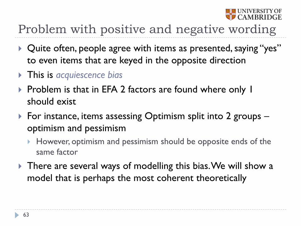
Quite often, people agree with items as presented, saying “yes”

to even items that are keyed in the opposite direction

This is acquiescence bias

Problem is that in EFA 2 factors are found where only 1

should exist

For instance, items assessing Optimism split into 2 groups –

optimism and pessimism

However, optimism and pessimism should be opposite ends of the

same factor

There are several ways of modelling this bias. We will show a

model that is perhaps the most coherent theoretically

Random intercept model

64

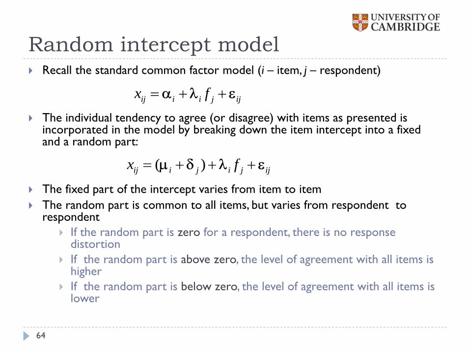
Recall the standard common factor model (i – item, j – respondent)

The individual tendency to agree (or disagree) with items as presented is incorporated in the model by breaking down the item intercept into a fixed and a random part:

The fixed part of the intercept varies from item to item

The random part is common to all items, but varies from respondent to respondent

If the random part is zero for a respondent, there is no response distortion

If the random part is above zero, the level of agreement with all items is higher

If the random part is below zero, the level of agreement with all items is lower

ij i i j ijx f

( )ij i j i j ijx f

Random intercept structural model

65

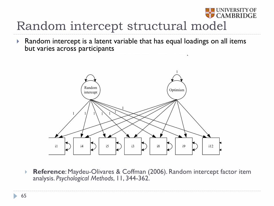
Random intercept is a latent variable that has equal loadings on all items but varies across participants

Reference: Maydeu-Olivares & Coffman (2006). Random intercept factor item analysis. Psychological Methods, 11, 344-362.

Example - Diversity scale

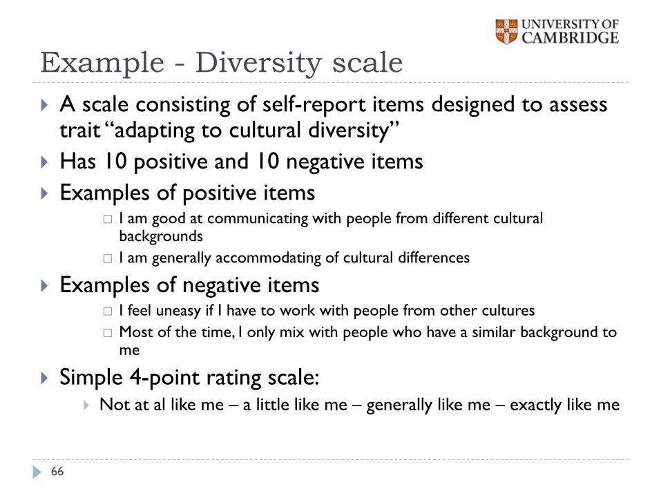
66

A scale consisting of self-report items designed to assess trait “adapting to cultural diversity”

Has 10 positive and 10 negative items

Examples of positive items I am good at communicating with people from different cultural

backgrounds

I am generally accommodating of cultural differences

Examples of negative items I feel uneasy if I have to work with people from other cultures

Most of the time, I only mix with people who have a similar background to me

Simple 4-point rating scale: Not at al like me – a little like me – generally like me – exactly like me

EFA of diversity scale

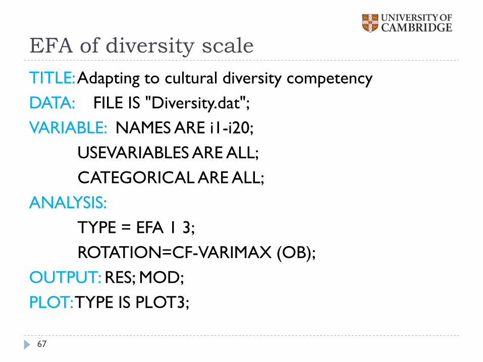
67

TITLE: Adapting to cultural diversity competency

DATA: FILE IS "Diversity.dat";

VARIABLE: NAMES ARE i1-i20;

USEVARIABLES ARE ALL;


ANALYSIS:

TYPE = EFA 1 3;


OUTPUT: RES; MOD;


Model results

68

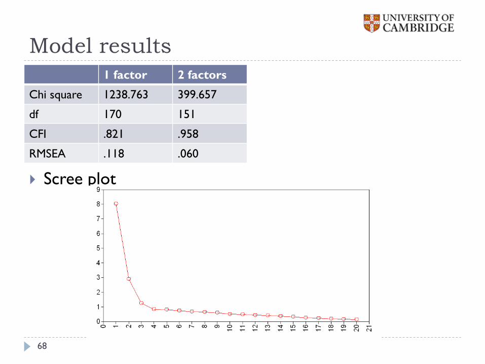
Scree plot

1 factor 2 factors

Chi square 1238.763 399.657

df 170 151

CFI .821 .958

RMSEA .118 .060

Syntax for the random intercept model

69

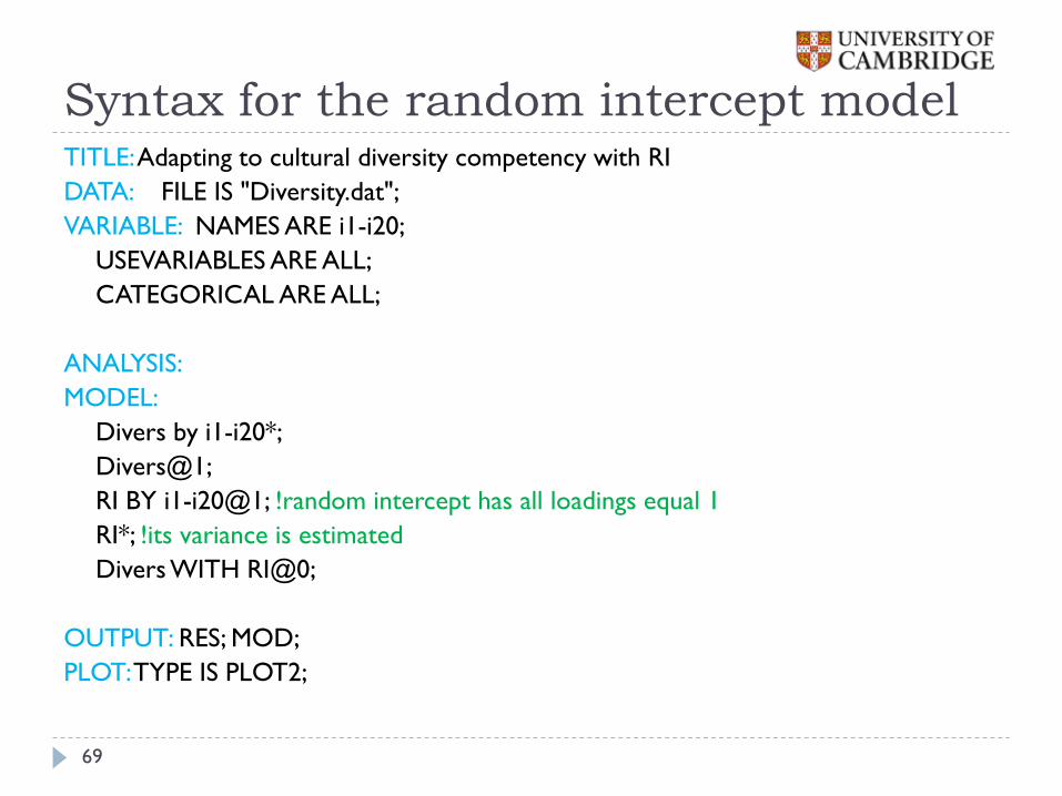
TITLE: Adapting to cultural diversity competency with RI

DATA: FILE IS "Diversity.dat";

VARIABLE: NAMES ARE i1-i20;

USEVARIABLES ARE ALL;


ANALYSIS:

MODEL:

Divers by i1-i20*;

Divers@1;

RI BY i1-i20@1; !random intercept has all loadings equal 1

RI*; !its variance is estimated

Divers WITH RI@0;

OUTPUT: RES; MOD;


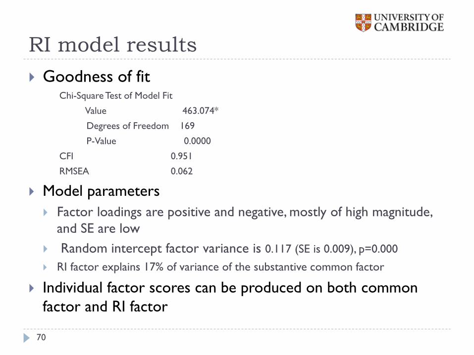
RI model results

70

Goodness of fit Chi-Square Test of Model Fit

Value 463.074*


P-Value 0.0000

CFI 0.951

RMSEA 0.062

Model parameters

Factor loadings are positive and negative, mostly of high magnitude,

and SE are low

Random intercept factor variance is 0.117 (SE is 0.009), p=0.000

RI factor explains 17% of variance of the substantive common factor

Individual factor scores can be produced on both common

factor and RI factor

Thank you

71

In these 2 days we have:

…learnt the principles of EFA and CFA

…applied these principles to real data

…practiced a lot of basic and not so basic analyses

…learnt how to use Mplus to perform these analyses

Further steps:

Practice to test these models with your own data

If you need help or further information, contact us

Jan Stochl

Anna Brown

Confirmatory factor analysis in - restore.ac.uk · Confirmatory factor analysis in ... Analysing...

Documents

Transcript of Confirmatory factor analysis in - restore.ac.uk · Confirmatory factor analysis in ... Analysing...