CONFERENCE FULL-PAPER PROCEEDINGS BOOK 1.pdf · Welcome to ICOAEF 2016 2nd International Conference...

CONFERENCE FULL-PAPER PROCEEDINGS

BOOK

2ND INTERNATIONAL CONFERENCE on

Applied Economics and Finance

(ICOAEF 2016)

5 - 6 December, 2016

Girne American University

North Cyprus

https://www.google.com.cy/url?sa=i&rct=j&q=&esrc=s&source=imgres&cd=&cad=rja&uact=8&ved=0ahUKEwiptJf58-vQAhWIC8AKHW9hBJAQjRwIBw&url=https://plus.google.com/114754895273645458412&psig=AFQjCNFhDERDIq3fdDGHiElL-ZcYM7pBWA&ust=1481537643109017

Welcome to ICOAEF 2016

2nd International Conference on Applied Economics and Finance (ICOAEF 2016) is the second

event in the series. We are proud to organise and host this event at the Girne American

University. ICOAEF 2016 provided an opportunity for all those interested in the Applied

Economics and Finance to discuss their research and to exchange ideas. We received papers

from all the following fields: Applied Macroeconomics, Applied Microeconomics, Applied

International Economics, Applied Energy Economics, Applied Financial Economics, Applied

Agricultural Economics, Applied Labour and Demographic Economics, Applied Health

Economics, Applied Education Economics, Applied International Trade, Econometrics, Applied

Statistics, Capital Markets, Corporate Finance, Quantitative Methods, Mathematical Finance,

Operations Research, Risk Management.

This year, we were together with about 140 young and experienced researchers, Ph.D. students,

post-doctoral researchers, academicians, and professionals from business, government and non-

governmental institutions from 24 different countries and enjoy about 130 presentations.

ICOAEF 2016 attracting such a high number of particiapts is a good indicator of the success and

means the conference serving its purpose and offer a good opportunity for scholarly exchange

and networking.

We thank Girne American University, again, for hosting ICOAEF 2016. We also thank the

Central Bank of the Republic of Turkey for their support and contribution to the Conference.

Dervis Kirikkaleli, PhD

Acting Dean, Business Faculty


Girne, North Cyprus

Email [email protected] / [email protected] / [email protected]

Mob: 00 90 548 863 77 70

mailto:[email protected]



i

TABLE OF CONTENTS

SPONSORS - - - - - - - - - i

GENERAL INFORMATION - - - - - - -ii

Organization Committee - - - - - - -ii

Scientific Committee - - - - - - - -ii

Contact - - - - - - - -iv

Halls - - - - - - - - -iv

PROGRAMME - - - - - - - -v - vii

SESSIONS - - - - - - - - -vii - xxiv

FULL PAPERS - - - - - - - - 28 - 407

Alla Mostepaniuk

• CONTRADICTIONS IN PUBLIC-PRIVATE PARTNERSHIP DEVELOPMENT

WITHIN TRANSITIONAL ECONOMIES - - -28- 41

Amin Sokhanvar, Iman Aghaei and Şule L. Aker

• THE EFFECT OF PROSPERITY ON INTERNATIONAL TOURISM

EXPENDITURES - - - - - - -42- 52

Bülent Günceler

• WHY “GLOBAL CRISIS” HIT TURKISH BANKING SYSTEM LESS THAN

OTHER COUNTRIES ? - - - - - -53 -61

Dlawar Mahdi Hadi

• INDUSTRIAL PRODUCTION, CO2 EMISSIONS AND FINANCIAL

DEVELOPMENT; A CASE FROM THAILAND - - -62- 69

Dogus Emin

• WHAT IS THE REAL REASON OF THE PROPOGATION OF FINANCIAL

CRISES AND HOW IT CAN BE STOPPED? - - - -70-78

Ebubekir Karaçayir

• THE RELATIONSHIP BETWEEN FOREIGN DIRECT INVESTMENT AND

INTRA INDUSTRY TRADE: AN EMPIRICAL ANALYSIS ON TURKEY AND

EU (15) COUNTRIES - - - - - - -79- 88

Elżbieta Grzegorczyk

• PRIVATE EQUITY/VENTURE CAPITAL IN HIGH-TECHNOLOGY SECTOR

- - - - - - - - -89- 111

Emre Atilgan

• THE PRINCIPAL-AGENT PROBLEM IN HEALTH CARE SYSTEMS: IS IT

EFFECTED BY PERFORMANCE-BASED SUPPLEMENTARY PAYMENT

- - - - - - - - -112-117

ii

Hakan Yaş and Emre Atilgan

• THE DETERMINANTS OF BORROWING BEHAVIORS OF TURKISH

MUNICIPALITIES - - - - - - - -118-126

Iman Aghaei, Amin Sokhanvar and Mustafa Tümer

• THE IMPORTANCE OF EFFECTIVE SOCIOECONOMIC CONDITIONS,

GOVERNMENT POLICIES AND PROCEDURES FACTORS FOR

ENTREPRENEURIAL ACTIVITY: (USING

FUZZY ANALYTIC HIERARCHY PROCESS IN EIGHT DEVELOPING

COUNTRIES) - - - - - - - -127-140

Mohammad Asif

• ENVIRONMENTAL KUZNET’S CURVE FOR SAUDI ARABIA: AN

ENDOGENOUS STRUCTURAL BREAKS BASED ON COINTEGRATION

ANALYSIS - - - - - - - - -141-155

Mustafa Daskin

• EXPLORING THE PERCEPTIONS OF TOURISM STUDENTS ABOUT

INDUSTRIAL CAREER: A PERSPECTIVE FROM TOURISM ECONOMICS OF

TOURISM INDUSTRY - - - - - - -156-166

Ayhan Kapusuzoglu and Nildag Basak Ceylan

• THE EFFECT OF FOREIGN BANK ENTRY ON THE FINANCIAL

PERFORMANCE OF THE COMMERCIAL BANKS IN TURKEY- -167-169

Panteha Farmanesh

• THE DEVELOPMENT OF E-COMMERCE AND THE INFLUENCE OF CONSUMER

CONFIDENCE ON THE ECONOMY OF IRAN. - -170-185

Parviz Piri, Samaneh Barzegari Sadaghiani and Fariba Abdeli Habashi

• THE RELATIONSHIP BETWEEN ELEMENTS OF INTERNAL FINANCIAL

FLEXIBILITY IN MARKET PARTICIPANT`S DECESION MAKING

- - - - - - - - -186-197

Faruk Demirhan, Mustafa Göktuğ Kaya and Perihan Hazel Kaya

• THE RELATIONSHIP BETWEEN FOREIGN DIRECT INVESTMENT,

ECONOMIC GROWTH AND UNEMPLOYMENT IN TURKEY: AN EMPIRICAL

ANALYSIS FOR THE PERIOD OF 2008-2015- - - -198-217

Serpil Gumustekin and Talat Senel

• EFFICIENCY ASSESSMENT OF THE TRANSPORTATION SERVICES IN

TURKEY - - - - - - - - -218-222

Tolga Zaman and Emre Yildirim

• FINANCIAL PERFORMANCE INVESTIGATION WITH THE HELP OF THE

BOOTSTRAP METHOD: AN EXAMPLE OF THE EREDIVISIE LEAGUE –

- - - - - - - - -223- 229

iii

Yaşar Serhat Yaşgül

• TESTING CONVERGENCE IN RESEARCH OUTPUT IN BIOTECHNOLOGY

FOR G7 COUNTRIES - - - - - - -230-235

Uğur Aytun and Yılmaz Kılıçaslan

• COMPLEXITY, COMPETITIVENESS AND TECHNOLOGY: IS THERE A LINK?

- - - - - - - - - -236-246

Yılmaz Toktaş and Eda Bozkurt

• THE ANALYSIS OF THE RELATIONSHIP BETWEEN TURKEY’S REAL

EFFECTIVE EXCHANGE RATE AND HAZELNUT EXPORT TO GERMANY

VIA BOUNDS TEST - - - - - - - -247- 254

Zeynep Karaçor and Duygu Baysal Kurt

• THE RELATIONSHIP OF CO2 EMISSION AND ECONOMIC GROWTH IN

BRICS-T COUNTRIES: A PANEL DATA ANALYSIS - - -255- 265

Zhiyar Ismael

• THE IMPACT OF BILATERAL INVESTMENT TREATIES (BITS) AS A

POLITICAL RISK MITIGATOR ON ATTRACTING FOREIGN DIRECT

INVESTMENT (FDI) - - - - - - -267-274

P. Sergius Koku, Besnik Fatai, Fitim Deari and Izet Zeqiri

• DO PRESS RELEASES PROVIDE NEW INFORMATION? THE CASE OF

BRITISH PETROLEUM‘S DEEPWATER HORIZON OIL SPILL - -275-278

Burak Sencer Atasoy and Esra Kabaklari

• THE EFFECTS OF DIGITAL ECONOMY ON PRODUCTIVITY: A DYNAMIC

PANEL DATA ANALYSIS- - - - - - -279 - 287

Fatih Ayhan and Fatih Mangir

• AN INVESTIGATION THE RELATIONSHIP BETWEEN THE EXCHANGE RATE

VOLATILITY AND TOURISM RECEIPTS FOR TURKISH ECONOMY -

- - - - - - - - -288 – 297

•

Siti Muawanah Lajis, and Abbas Mirakhor,

• RISK-SHARING BANKING: VIABILITY AND RESILIENCE -298 – 317

Adnan Celik and Sadife Gungor

• EMPLOYEES OF STRESS LEVELS, THE EFFECT OF JOB SATISFACTION: A

FIELD STUDY - - - - - - - -318 – 328

Adnan Celik, Emine Et Oltulu and Hevhan Ozgu Cakir

• THE EFFECT OF ETHICAL CLIMATE PERCEPTION OF TEACHERS TO THEIR

ORGANIZATIONAL COMMITMENT: A SAMPLE PRACTICE - -329 – 340

iv

Malgorzata Jablonska

• POSITION OF ENTREPRENEURSHIP IN THE FINANCIAL PERSPECTIVE 2007

– 2013. AN EXAMPLE OF CENTRAL POLAN - - - -341 – 350

Orhan Coban and Nihat Doganalp

• THE EFFECT ON MACRO ECONOMIC INDICATORS OF THE FINANCIAL

CRISIS AS A PARADOX OF NEOLIBERALISM: THE CASE OF TRNC - 351 – 361

Nihat Doganalp and Ayse Coban

• IN THE WORLD AND TURKEY, EXPERIENCES OF FINANCIAL CRISIS: A

COMPARISON ON THE AXIS OF FINANCIAL CRISIS MODEL - -362 – 376

Hasan Bulut and Yuksel Oner

• COMPARISON OF THE SOCIO-ECONOMIC DEVELOPMENT AND THE PISA

RESULTS OF OECD COUNTRIES. - - - - - -377-381

Sefa Cetin, Hasan Huseyin Buyukbayraktar and Abdullah Yilmaz

• OBSTACLES IMMIGRANTS FACED IN INTEGRATION TO LABOR MARKET:

THE SAMPLE OF SYRIAN IMMIGRANTS IN TURKEY - - -382 – 399

Nadir Eroglu, Imran Emre Kragozlu, and Ahmet Akca

• HEDGING OIL PRICE RISK BETWEEN OIL IMPORTER AND OIL EXPORTER

COUNTRIES: A CASE STUDY FOR TURKEY AND MEXICO

- - - - - - - - - - -400- 407

Mohammadreza Allahverdian, Mohammad Rajabi, and Mohsen Mortazavi

• EDUCATION LEVEL AND ECONOMIC GROWTH: THE EUROPEAN

EXPERIENCE - - - - - - - 408 - 422

Mohammad Rajabi and Mohammadreza Allahverdian

• THE NEXUS BETWEEN CO2 EMISSIONS, ECONOMIC GROWTH AND ENERGY

CONSUMPTION: EMPIRICAL EVIDENCE FROM MINT COUNTRIES. - - - - - - - - - - 423 - 435

v

SPONSORS

This conference is funded by Central Bank of the Republic of Turkey

Edited by Derviş Kırıkkaleli,

Faculty of Business,

Girne American University, Cypurs.

Published by Anglo-American Publications LLC

3422 Old Capitol Trail, Suite 700, Wilmington,

Delaware,19808-6192, USA.

Telephone: (302)3803-692

E-mail : [email protected]

Abstracting and nonprofit use of the material is permitted with credit to the source. Instructors

are permitted to photocopy isolated articles for noncommercial use without fee. Any

republication or personal use of the work must explicitly identify prior publication in

Proceedings of Abstracts and Papers (on e-book) of the 2nd International Conference on Applied

Economics and Finance 2016, including the page numbers.

Proceedings of Abstracts and Papers (on e-book) of The 2nd International Conference on Applied

Economics and Finance 2016

Copyright©2016

By Derviş Kırıkkaleli, GAU Journal of Social and Applied Sciences; Girne American University,

Cyprus.

All rights reserved.

All papers in the proceedings have been peer reviewed by experts in the respective fields.

Responsibility for the contents of these papers rests upon the authors.

ISBN: 978-1-946782-01-4

Published by Anglo-American Publications LLC, 3422 Old Capitol Trail, Suite 700,

Wilmington, Delaware,19808-6192, USA.

vi

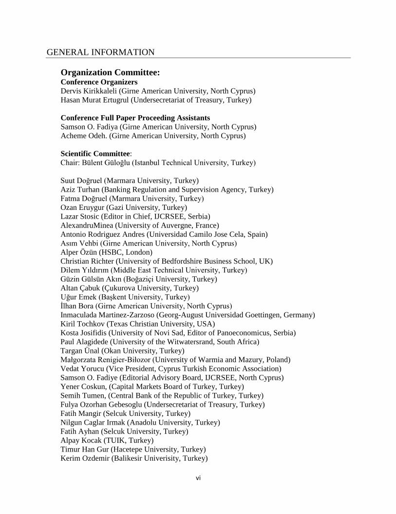
GENERAL INFORMATION

Organization Committee: Conference Organizers

Dervis Kirikkaleli (Girne American University, North Cyprus)

Hasan Murat Ertugrul (Undersecretariat of Treasury, Turkey)

Conference Full Paper Proceeding Assistants

Samson O. Fadiya (Girne American University, North Cyprus)

Acheme Odeh. (Girne American University, North Cyprus)

Scientific Committee:

Chair: Bülent Güloğlu (Istanbul Technical University, Turkey)

Suut Doğruel (Marmara University, Turkey)

Aziz Turhan (Banking Regulation and Supervision Agency, Turkey)

Fatma Doğruel (Marmara University, Turkey)

Ozan Eruygur (Gazi University, Turkey)

Lazar Stosic (Editor in Chief, IJCRSEE, Serbia)

AlexandruMinea (University of Auvergne, France)

Antonio Rodriguez Andres (Universidad Camilo Jose Cela, Spain)

Asım Vehbi (Girne American University, North Cyprus)

Alper Özün (HSBC, London)

Christian Richter (University of Bedfordshire Business School, UK)

Dilem Yıldırım (Middle East Technical University, Turkey)

Güzin Gülsün Akın (Boğaziçi University, Turkey)

Altan Çabuk (Çukurova University, Turkey)

Uğur Emek (Başkent University, Turkey)

İlhan Bora (Girne American University, North Cyprus)

Inmaculada Martinez-Zarzoso (Georg-August Universidad Goettingen, Germany)

Kiril Tochkov (Texas Christian University, USA)

Kosta Josifidis (University of Novi Sad, Editor of Panoeconomicus, Serbia)

Paul Alagidede (University of the Witwatersrand, South Africa)

Targan Ünal (Okan University, Turkey)

Małgorzata Renigier-Biłozor (University of Warmia and Mazury, Poland)

Vedat Yorucu (Vice President, Cyprus Turkish Economic Association)

Samson O. Fadiye (Editorial Advisory Board, IJCRSEE, North Cyprus)

Yener Coskun, (Capital Markets Board of Turkey, Turkey)

Semih Tumen, (Central Bank of the Republic of Turkey, Turkey)

Fulya Ozorhan Gebesoglu (Undersecretariat of Treasury, Turkey)

Fatih Mangir (Selcuk University, Turkey)

Nilgun Caglar Irmak (Anadolu University, Turkey)

Fatih Ayhan (Selcuk University, Turkey)

Alpay Kocak (TUIK, Turkey)

Timur Han Gur (Hacetepe University, Turkey)

Kerim Ozdemir (Balikesir Univerisity, Turkey)

vii

Ercan Saridogan (Istanbul University, Turkey)

Burchan Sakarya (BDDK, Turkey)

Emre Atilgan (Trakya University, Turkey)

Yilmaz Kilicaslan (Anadolu University, Turkey)

Burak Daruci Bandirma (Onyedi Eylul Univeristy, Turkey)

Ugur Soytas (METU, Turkey)

Mehmet Ali Soytas (Ozyegin University, Turkey)

Ali Alp (TOBB University of Economics and Technology, Turkey)

Nadir Ocal (METU, Turkey)

Dilvin Taskin (Yasar University, Turkey)

Kemal Yildirim (Anadolu University, Turkey)

Selim Yildirim (Anadolu University, Turkey)

Onur Baycan (Anadolu University, Turkey)

Ahmet Ay (Selcuk University, Turkey)

Ramazan Sarı, (METU, Turkey)

Mehmet Şişman (Marmara University, Turkey)

Ünal Seven (TCMB, Turkey)

Deniz Şişman (Gelişim University, Turkey)

Aykut Lenger (Ege University, Turkey)

Paloma Taltavull de La Paz , ( University of Alicante , Spain)

Maurizio D'amato, (Technical University of Politecnico di Bari, Italy)

Omokolade Akinsomi, (University of the Witwatersrand, Güney Afrika)

Charalambos Pitros, ( University of Salford , United Kingdom)

Ong Seow Eng, (National University of Singapore, Singapore)

Noorsidi Aizuddin Bin Mat Noor , (Universiti Teknologi Malaysia, Malaysia)

Rangan Gupta (University of Pretoria, South Africa)

Anil K. Bera (University of Illinois, USA)

Jasmin Hoso (American University, USA)

Micheal Scroeder (Centre for European Economic Research, Germany)

Jan Černohorský (University of Pardubice, Czech Republic)

Martin Hnízdo (University of Pardubice, Czech Republic)

Shekar Shetty (Gulf University for Science & Technology, Kuwait)

Mansour AlShamali (Public Authority for Applied Education and Training, Kuwait)

Nizar Yousef Naim (Ahlia University, Kingdom of Bahrain)

Djula Borozan (University of Osijek, Croatia)

Mirjana Radman Funaric (Polytechnic in Pozega, Croatia)

P. Sergius Koku (Florida Atlantic University/South East European University)

Besnik Fetai (South Eastern European University, Macedonia)

Małgorzata Jabłońska (University of Lodz, Poland)

Abdelfeteh Bitat (Universite Saint-Louis Bruxelles, Belgium)

Snežana Todosijević - Lazović (University of Priština, Faculty of Economics Mitrovica, R.

Kosovo)

Zoran Katanic (High School of Economics Peć in Leposavić, R. Kosovo)

Abbas Mirakhor (International Centre for Education in Islamic Finance, Malaysia)

Wool Shin (Samsung Group, Korea)

Siti Muawanah Lajis (Bank Negara Malaysia)

viii

Alaa Alabed (International Centre for Education in Islamic Finance, Malaysia)

Alex Petersen (the University of California, USA)

Alessandro Belmonte (IMT School for Advanced Studies Lucca, Italy)

Carlo Del Maso (BTO Research, Italy)

Andrea Flori, (IMT School for Advanced Studies Lucca, Italy)

Emi Ferra (IMT School for Advanced Studies Lucca, Italy)

Rodolfo Metulini (Universita Degli Studi di Brescia, Italy)

Liang Peng (Penn State University, USA)

Contact: Dervis Kirikkaleli

Acting Dean, Business Faculty

Girne American University, Girne

North Cyprus

Email [email protected] / [email protected] / [email protected]

Mob: 00 90 548 863 77 70

Halls: 1. Milenium Senato Hall

2. A3.2 Room

3. A3.3 Room

4. A3.4 Room

5. A3.5 Room

6. A3.6 Room




ix

PROGRAM

5th December, Monday 08:00-9:30 REGISTRATION

09.30-11.00 KEYNOTE SPEAKERS SESSION

Room: Milenium Senato Hall, GAU

1. Kutsal Öztürk

2. Asım Vehbi 3. Badi H. Baltagi 4. Talat Ulusever 5. Yakup Asarkaya

6. Alper Özün

11.00 – 11.30 Coffee Break

11.30-13.00 SPECIAL SESSIONS

Turkısh Economy [Room: Milenium Senato Hall, GAU]

13:00-14:00 Lunch

14.00-15.30 SESSIONS

1. Islamic Finance. [Room: A3.2]

2. Uygulamalı Ekonomi ve Finans I. (Dil : Türkçe). [Room: A3.3]

3. Applied Finance. [Room: A3.4]

4. Energy Economics [Room: A3.5]

15.30-16.00 Coffee Break


1. Investment. [Room: A3.2]

2. Uygulamalı Ekonomi ve Finans II. (Dil : Türkçe) [Room A3.3]

3. Economic Development I [Room: A3.4]

4. Monetary Policy [Room: A3.5]

5. Multidisciplinary I [Room: A3.6]

19.30-21.00 Gala Dinner in Le Chateau Lambousa Hotel

x

6th December, Monday

9.30-11.00 SESSIONS

1. International Trade [Room: A3.2]

2. Multidisciplinary II [Room: A3.3]

3. Applied Microeconomics [Room: A3.4]

4. Applied Econometrics and Statistics [Room: A3.5]



1. Business Economics [Room: A3.2 ]

2. Uygulamalı Ekonomi ve Finans III. (Dil : Türkçe) [Room: A3.3]

3. Energy Economics II [Room: A3.4]

4. Tourism Economics [Room: A3.5]

5. Health Economics [Room: A3.6]

13.00-14.00 Lunch Break


1. Uygulamalı Ekonomi ve Finans IV. (Dil : Türkçe) [Room: A3.3 ]

2. Financial Crisis and Stability [Room: A3.2]

3. Educaiton Economics and Labour Market [Room: A3.2]

4. Applied Banking [Room: A3.5]

5. Applied Banking II [Room: A3.6]



1. Multidisciplinary III [Room: A3.2]

2. Uygulamalı Ekonomi ve Finans V. (Dil : Türkçe) [Room: A3.3]

3. Economic Development II [Room: A3.4]

4. Applied Finance II [Room: A3.5]

5. Energy Economics III [Room: A3.6]

xi

SESSIONS

2nd International Conference on Applied Economics and Finance

5-6 December, 2016

Girne American University, North Cyprus

Organized by

Derviş Kırıkkaleli (Girne American University, North Cyprus)

Hasan Murat Ertuğrul (Undersecretariat of Treasury, Turkey)

Program

Keynote Speakers Session


Time: 05.12.2016, 09.30-11.00

Openning Speach: Kutsal Öztürk (Rector, Girne American University, North Cyprus)

Asım Vehbi (Vice Chancellor, Girne American University, North Cyprus)

1) Badi H. Baltagi (Syracuse University, USA)

2) Talat Ulusever (Acting President, Capital Market of Turkey, Turkey)

3) Yakup Asarkaya (Vice President, Banking Regulation and Supervision Agency, Turkey)

4) Alper Özün (Director, HSBC Global, UK)

Moderator: Lazar Stosic (Editor in Chief, IJCRSEE, Serbia)

Guest: Kerim Özdemir (Rector, Balıkesir University, Turkey)

Coffee Break 11.00 – 11.30

Special Session: Turkish Economy


Time: 05.12.2016, 11.30-13.00

1) Ramazan Sarı (Middle East Technical University, Turkey)

Recent Developments in Energy Markets and Turkey's Energy Outlook

2) Yener Coşkun (Capital Market of Turkey, Turkey)

Recent Developments in Housing Markets and Housing Market in Turkey

3) Yilmaz Kılıçaslan (Anadolu University, Turkey)

What's Wrong with Turkish Economy? Growth, Productivity and Industrial Structure

Moderator: Bulent Guloglu (Istanbul Technical University, Turkey)

xii

Lunch 13.00-14.00

Islamic Finance

Room: A3.2 Room, GAU

Time: 05.12.2016, 14.00-15.30

1) Accelerating Risk Sharing Finance via Fintech: Nextgen Islamic Finance

Alaa Alaabed ( INCEIF, Malaysia)

Siti Muawanah Lajis (The Central Bank Of Malaysia, Malaysia)

2) Gender Effects On Service Quality, Customer Satisfaction And Loyalty In Islamic Banks

Of Sudan

Berna Serener (Near East University, North Cyprus)

3) Lack of Standardization in Sukuk Market

Ahmet Ulusoy (Karadeniz Techinacal University, Turkey)

Mehmet Ela (Osmaniye Korkut Ata University, Turkey)

4) Risk-Sharing Banking: Viability and Resilience

Siti Muawanah Lajis (The Central Bank of Malaysia, Malaysia)

Abbas Mirakhor (INCEIF,Malaysia)

5) Financial Performance of Islamic Bank vs Conventional Banks: The Case of UAE

Nesrin Ozatac (Eastern Mediterranean University, North Cyprus)

Oubayda El Rifai (Eastern Mediterranean University, North Cyprus)

Chair: Seyed Alireza Athari (Girne American University, North Cyprus)

Uygulamalı Ekonomi ve Finans I. (Dil : Türkçe)


Time: 05.12.2016, 14.00-15.30

1) Küresel Finans Ve “Yüksek Etkileşimli” Şirketler

Mehmet Şişman (Marmara University, Turkey)

Deniz Şişman (Gelişim University, Turkey)

2) Türkiye'de Beseri Sermayenin Yoksullukla Mucadele ve Gelir Dagılımı Uzerindeki

Etkileri

Ferhat Pehlivanoğlu (Kocaeli University, Turkey)

Sema Yilmaz Genç (Kocaeli University, Turkey)

3) Türkiye’de İç Göçü Etkileyen Faktörler Üzerine Bir Uygulama: Mekânsal Panel Veri

Analizi

Gökçe Manavgat (Ege University, Turkey)

R. Fatih Saygili (Ege University, Turkey)

4) Thirlwall Kanunu: OECD Ülkeleri Örneği, 1990-2014

xiii

Fatih Mangır (Selcuk University, Turkey)


Ş.Süreyya Kodaz (Selcuk University, Turkey)

Chair: Mehmet Şişman (Marmara University, Turkey)

Applied Finance I


Time: 05.12.2016, 14.00-15.30

1) Optimal Surrender of Guaranteed Minimum Maturity Benefits under Stochastic Volatility

and Interest Rates

Jonathan Ziveyi (UNSW Business School, Australia)

Boda Kang (University of York, England)

2) Volatility Transmission among Commodity and Stock Markets: Evidence from

Developed and Developing Countries

Gülin Vardar (Izmir University of Economics, Turkey)

Yener Coşkun (Capital Markets of Turkey, Turkey)

Tezer Yelkenci (Izmir University of Economics, Turkey)

3) Private Equity/Venture Capital in High-Technology Sector

Elżbieta Grzegorczyk (University of Lodz, Poland )

4) Financial Contagion, Flight To Quality And Flight From The Quality Among The Stock

Exchange Markets Of Turkey And The Developed And The Developing Countries

Pinar Kaya(Marmara University, Turkey)

Bulent Guloglu (Istanbul Technical University, Turkey)

5) Diversification Benefit and Return Performance of REITs Using CAPM and Fama-

French: Evidences from Turkey

Yener Coşkun (Capital Markets of Turkey, Turkey)

Ayse Sevtap Kestel (Middle East Technical University, Turkey)

Bilgi Yilmaz(Middle East Technical University, Turkey)

Chair: Bulent Guloglu (Istanbul Technical University, Turkey)

Energy Economics I


Time: 05.12.2016, 14.00-15.30

1) Industrial Production, Co2 Emissions Financial Development; a Case from Thailand

Dlawar Mahdi Hadi (Eastern Mediterranean University, North Cyprus)

2) The Nexus between CO2 emissions, Economic Growth and Energy Consumption:

Empirical Evidence from MINT countries

Mohammad Rajabi (Eastern Mediterranean University, North Cyprus)

xiv

Mohammadreza Allahverdian (Eastern Mediterranean University, North Cyprus)

3) Bubble Detection in US Energy Market: Application of Log Periodic Power Law Models

Andisheh Saliminezhad (Eastern Mediterranean University, North Cyprus)

Pejman Bahramian (Eastern Mediterranean University, North Cyprus)

4) Hedging Oil Price Risk Between Oil Importer And Oil Exporter Countries, a Case Study

for Turkey and Mexico

Nadir Eroğlu (Marmara University, Turkey)

İmran Emre Karagözlü (Marmara University, Turkey)

Ahmet Akça (Bahçeşehir University, Turkey)

5) An Investigation of the Effect of Oil Price on Russian Economy

Esra Balli (Cukurova University, Turkey)

Chair: Hüsnü Tekin (Istanbul University, Turkey)

Coffee Break 15.30-16.00

Investment


Time: 05.12.2016, 16.00-17.30

1) The Relationship Between Foreign Direct Investment and Intra Industry Trade: An

Empirical Analysis on Turkey and EU (15) Countries

Ebubekir Karacayir (Karamanoğlu Mehmetbey University, Turkey)

2) Determinants of Foreign Direct Investments in the CEECS after EU Accession

Gulcin Guresci Pehlivan (Dokuz Eylül University, Turkey)

Esra Balli (Cukurova University, Turkey)

3) The Relationship between Foreign Direct Investment, Economic Growth and

Unemployment In Turkey: An Empirical Analysis for the Period of 2008-2015

Faruk Demirhan (Tax Inspection Board, Turkey)

Mustafa Göktuğ Kaya (Tax Inspection Board, Turkey)

Perihan Hazel Kaya (Selçuk University, Turkey)

4) FDI, Industrial Production and Economic Growth; A case from Egypt


5) The Impact of Bilateral Investment Treaties (BITS) as a Political Risk Mitigator on

Attracting Foreign Direct Investment (FDI)

Zhiyar Ismael (Girne American University, North Cyprus)

Chair: Dilber Caglar (Girne American University, North Cyprus)

xv

Uygulamalı Ekonomi ve Finans II. (Dil : Türkçe)


Time: 05.12.2016, 16.00-17.30

1) Türkiye'deki Sistemik Öneme Sahip Bankaların Kantil Regresyon Kullanılarak CoVaR

(Koşullu Riske Maruz Değer) Yöntemi İle Tespit Edilmesi

Zehra Civan (Yildiz Technical University, Turkey)

Gülhayat Gölbaşi Şimşek (Yildiz Technical University, Turkey)

Ebru Çağlayan Akay (Marmara University, Turkey)

2) Carry Trade (Ara Kazanç) Strateji Ve Belirleyicileri Üzerine Bir Çalişma

Burçhan Sakarya (Banking Regulation and Supervision Agency, Turkey)

Ferhun Ateş (Banking Regulation and Supervision Agency, Turkey)

3) Evaluation of Tourism Efficiency by Malmquist Data Envelopment Analysis: A Case

Study of Cities In Turkey Ayhan Aydin (Adnan Menderes University, Turkey)

Serpil Gümüştekin (Ondokuz Mayıs University, Turkey.)

4) Türkiye’de İstihdamın Kuşaklara Göre Analizi

Fatih Çakmak (Kastamonu University, Turkey)

Mehmet Yunus Çelik (Kastamonu University, Turkey)

Chair: Ferhat Pehlivanoğlu (Kocaeli University, Turkey)

Economic Development I.


Time: 05.12.2016, 16.00-17.30

1) Exploring the Role of the Stages of Development on the Effects of Institutional Quality

on Economic Growth.

Seyed Alireza Athari (Girne American University, North Cyprus)

2) Effects of Volatility on Economic Growth: Evidence from the European Union


3) Measuring the Development Level and the Performance of Countries on Achieving

Millennium Development Goals

Ergül Halisçelik (Undersecretariat of Treasury, Turkey)

4) Causal Interactions between Economic Growth, Inflation and Stock Market

Development: The Case of Turkey

Nigar Taspinar (Eastern Mediterranean University, North Cyprus)

Bezhan Rustamov (Eastern Mediterranean University, North Cyprus)

Barış Eren (Eastern Mediterranean University, North Cyprus)

xvi

5) Capital Market-Growth Nexus: Evidence from Turkey

Yener Coşkun (Capital Market of Turkey, Turkey)

Ünal Seven (Central Bank of the Republic of Turkey, Turkey)

Talat Ulusever (Acting President, Capital Market of Turkey, Turkey)

Hasan Murat Ertuğrul (Undersecretariat of Treasury, Turkey)

Chair: Ergül Halisçelik (Undersecretariat of Treasury, Turkey)

Monetary Policy


Time: 05.12.2016, 16.00-17.30

1) Common Currency Unit for Gulf Cooperation Council:

Is it Feasible?

Shekar Shetty (Gulf University for Science & Technology, Kuwait)

Mansour AlShamali (Public Authority for Applied Education and Training, Kuwait)

2) Asymmetries in Monetary Policy Reaction Function and the Role of Uncertainties: The

Case of Turkey

Pelin Öge Güneya (Hacettepe University, Turkey)

3) The Relationship Between Exchange Rate and Inflation: The Case of

Western Balkans Countries

Besnik Fetai (South East European University, Republic of Macedonia)

Paul Sergius Koku (Florida Atlantic University/South East European University)

Agron Caushi (South East European University, Republic of Macedonia)

Chair: Vedat Yorucu (Eastern Mediterranean University, North Cyprus)

Multidisciplinary I


Time: 05.12.2016, 16.00-17.30

1) Profitability Forecast with Use of Meta Model Approach: the Case of Assessment of

Investment Project in Banking

Piotr Miszczynski (University Of Lodz, Poland)

2) Promoting Turkey’s Development: The Role Of Islamic Financial Instruments

Hüsnü Tekin (Istanbul University, Turkey)

3) The Performance of Health Care Sector: the Case of OECD Countries

Katarzyna Miszczyńska (University Of Lodz, Poland)

4) Sustainability of Public Deficits and Debt in Turkey

Selim Yildirim (Anadolu University, Turkey)

Fatih Temizel (Anadolu University, Turkey)

Ethem Esen (Anadolu University, Turkey)

xvii

S. Fatih Kostakoğlu (Anadolu University, Turkey)

Mehmet Dinç (Anadolu University, Turkey)

5) Employment Relations Challenges in Public Sector: Evidence From European Member

States

Ana-Maria BERCU (Alexandru Ioan Cuza University of Iasi, Romania)

Chair: Alla Mostepaniuk (Girne American University, North Cyprus)

Gala Dinner in Le Chateau Lambousa Hotel 19.30 - 21.00

International Trade


Time: 06.12.2016, 9.30-11.00

1) Application of Destination Brand Equity Model as an Economic Development Tool

Çağatan Taşkin (Uludağ University, Turkey)

2) Examining The Relationship Between Inflation Rates And Import: An Example in

Turkey

Mehmet Ali Cengiz (Ondokuz Mayıs University, Turkey)

Emre Dünder (Ondokuz Mayıs University,Turkey)

3) Interactions Between Financial Sector Development and International Trade Openness

On The Size Of Underground Economy: Empirical Evidence From European Union

Countries

Hatice Imamoglu (Eastern Mediterranean University, North Cyprus)

4) Outward Direct Investments of Turkish Firms

Yılmaz Kiliçaslan (Anadolu University, Turkey)

Zeynep Karal(Anadolu University, Turkey)

Gökhan Önder(Anadolu University, Turkey)

Yeşim Üçdoğruk(Dokuz Eylul University, Turkey)

Chair: Yılmaz Kiliçaslan (Anadolu University, Turkey)

Multidisciplinary II


Time: 06.12.2016, 9.30-11.00

1) British Petroleum‘s Deepwater Horizon Oil Spill: Do Press Releases Provide New

Information?

P. Sergius Koku (Florida Atlantic University, Macedonia)

xviii

Besnic Fetai (South Eastern European University, Macedonia)

Fitim Deari (South Eastern European University, Macedonia)

Izet Zeqiri (South East European University, Republic of Macedonia)

2) Satisfaction with Democracy in Latin America: Do the Characteristics of the Political

System Matter?

Selim Jürgen Ergun (Middle East Technical University, Northern Cyprus Campus)

M. Fernanda Rivas (Middle East Technical University, Northern Cyprus Campus)

Máximo Rossi (University of the Republic, Uruguay)

3) Evolution of Corporate Reporting – The Case of Polish Listed Companies

Dariusz Jedrzejka (University Of Lodz, Poland)

4) Modeling the Nonlinear Dynamics of the Turkish Unemployment Rates

Ismail Onur Baycan (Anadolu University, Turkey)

Chair: Ilhan Bora (Girne American University, North Cyprus)

Applied Microeconomics


Time: 06.12.2016, 9.30-11.00

1) Estimating the Constant Elasticity of Substitution Function of Rice Production. The Case

of Vietnam in 2012.

Linh K. Bui (Institute of World Economics and Politics, Vietnam Academy of Social

Sciences)

Huyen N. Hoang, (Crawford School of Public Policy, Australia)

Hang T. Bui (Vietnam Centre for Sustainable Rural Development, Vietnam)

2) The Effects of Digital Economy on Productivity: A Dynamic Panel Data Analysis

Esra Kabaklarli (Selçuk University, Turkey)

Burak Sencer Atasoy (Undersecretariat of Treasury, Turkey)

3) Short Term Investment Behavior of Turkish Manufacturing Sector: Evidence from BIST

Quoted Firms

Omer Tuğsal Doruk (American University of Cyprus & Kadir Has University, Turkey)

4) Consumption And Income Inequality in Turkey

Egemen İpek (Gumushane University, Turkey)

Chair: Aliya Zhakanova Isiksal (Girne American University, North Cyprus)

Applied Econometrics and Statistics


Time: 06.12.2016, 9.30-11.00

xix

1) A Comparison of MCMC Convergence Diagnostics and Goodness of Fit Index For

Diagnostics

Naci Murat (Ondokuz Mayis University, Turkey)

Emre Dünder, (Ondokuz Mayis University, Turkey)

Mehmet Ali Cengiz (Ondokuz Mayis University, Turkey)

2) Financial Performance Investigation with the Help of the Bootstrap Method: Example of

the Eredivisie League

Tolga Zaman (Ondokuz Mayıs University, Turkey)

Emre Yildirim (Ondokuz Mayıs University, Turkey)

3) Forecasting the Turkish Inflation Rate Using Information Criteria

Naci Murat (Ondokuz Mayis University, Turkey)

Emre Dünder (Ondokuz Mayıs University, Turkey)


4) A Dynamic Model of Turkish Electricity Prices

Mehmet Soytas (Ozyegin University, Turkey)

Chair: Emre Atılgan (Trakya University, Turkey)


Business Economics


Time: 06.12.2016, 11.30-13.00

1) Complexity, Competitiveness And Technology:

Is There A Link?

Yılmaz Kılıçaslan (Anadolu University, Turkey)

Uğur Aytun (Anadolu University, Turkey)

2) Employees of Stress Levels, The Effect of Job Satisfaction: A Field Study

Adnan Çelik (Selcuk University, Turkey)

Sadife Güngör (Selcuk University, Turkey)

3) An Experimental Approache to Rationality of Consumer Behavior

Ozlem Sekmen (Gumushane University, Turkey)

Haydar Akyazi(Gumushane University, Turkey)

Egemen İpek (Gumushane University, Turkey)

4) The Importance of Effective Socioeconomic Conditions, Government Policies and

Procedures Factors for Entrepreneurial Activity using Fuzzy Analytic Hierarchy Process

in Eight Developing Countries

Iman Aghaei (Eastern Mediterranean University, North Cypurs)

Amin Sokhanvar (Eastern Mediterranean University, North Cypurs)

xx

Mustafa Tümer (Eastern Mediterranean University, North Cypurs)

Chair: Yılmaz Kılıçaslan (Anadolu University, Turkey)

Uygulamalı Ekonomi ve Finans III. (Dil : Türkçe)


Time: 06.12.2016, 11.30-13.00

1) Modelling of Dependency Between Industrial Production Indexes and Their

Fundamentals Using Stochastic Copula Approach



1) The Effect On Macro Economic Indicators Of The Financial Crisis As A Paradox Of

Neoliberalism: The Case Of Trnc

Orhan Çoban(Selcuk University, Turkey)

Nihat Doğanalp (Selcuk University, Turkey)

2) Gümrük Birliği ve Helsinki Zirvesi’nin AB Üyelik Sürecinde Türkiye ve KKTC

Açisindan Değerlendirilmesi

Behive Çavuşoğlu (Near East University, North Cyprus)

Chair: Sema Yilmaz Genç (Kocaeli University, Turkey)

Energy Economics II


Time: 06.12.2016, 11.30-13.00

1) What Are the Dynamics of Co2 Emissions in Upper – Middle Income Countries? A Case

Study For China, Iran And Turkey

Hasan Rüstemoğlu (Cyprus International University, North Cyprus)

2) Environmental Kuznet’s Curve for Saudi Arabia: An Endogenous Structural Breaks

Based on Cointegration Analysis

Mohammad Asif (Aligarh Muslim University, India)

3) The Effect of Ethical Climate Perception of Teachers to Their Organizational

Commitment: A Sample Practice

Adnan Celik (Selçuk University, Turkey)

Emine Et Oltulu (Selçuk University, Turkey)

Beyhan Ozgu Cakir (Karatay University, Turkey)

4) Sectoral Impact of Crude Oil Price Shocks on Stock Returns in Selected Crude Oil

Exporting and Importing Emerging Economics.

Isah Wada (Eastern Mediterranean University, North Cyprus)

Gulcay Tuna (Eastern Mediterranean University, North Cyprus)

xxi

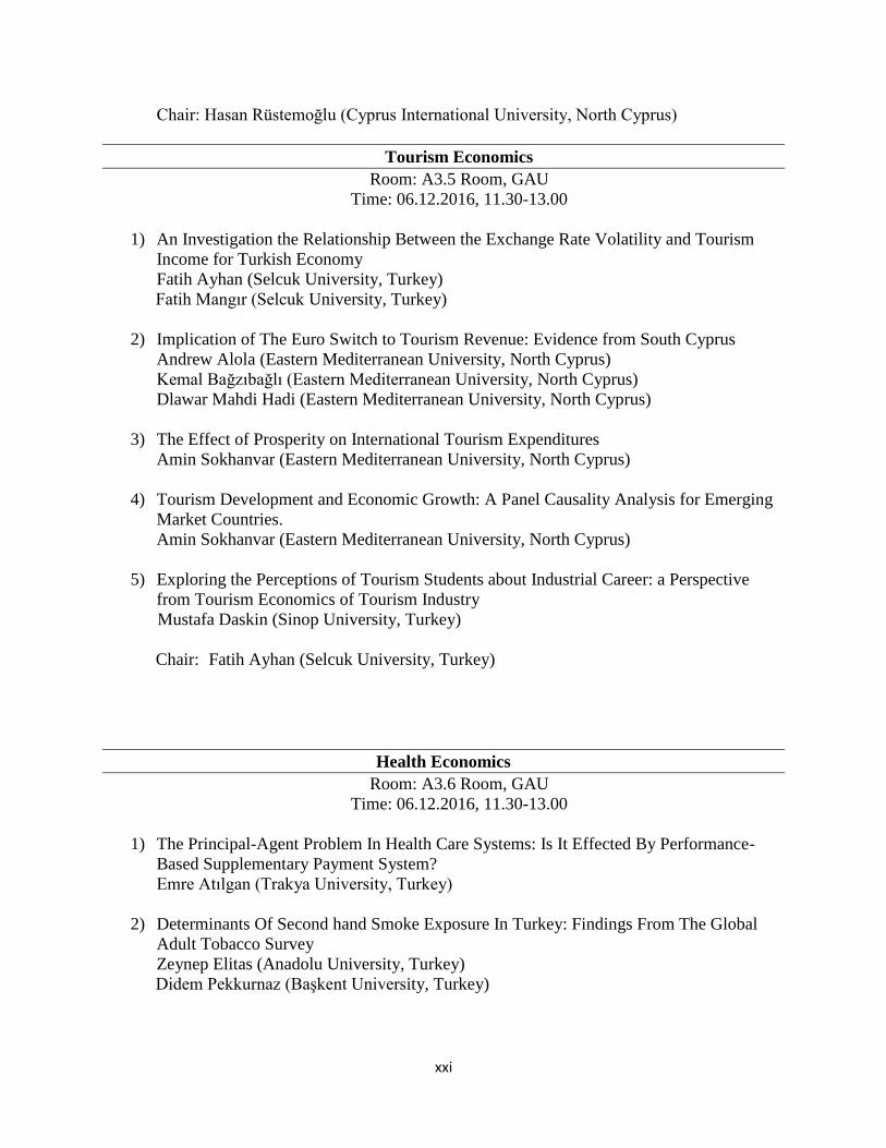
Chair: Hasan Rüstemoğlu (Cyprus International University, North Cyprus)

Tourism Economics


Time: 06.12.2016, 11.30-13.00

1) An Investigation the Relationship Between the Exchange Rate Volatility and Tourism

Income for Turkish Economy


Fatih Mangır (Selcuk University, Turkey)

2) Implication of The Euro Switch to Tourism Revenue: Evidence from South Cyprus

Andrew Alola (Eastern Mediterranean University, North Cyprus)

Kemal Bağzıbağlı (Eastern Mediterranean University, North Cyprus)


3) The Effect of Prosperity on International Tourism Expenditures

Amin Sokhanvar (Eastern Mediterranean University, North Cyprus)

4) Tourism Development and Economic Growth: A Panel Causality Analysis for Emerging

Market Countries.

Amin Sokhanvar (Eastern Mediterranean University, North Cyprus)

5) Exploring the Perceptions of Tourism Students about Industrial Career: a Perspective

from Tourism Economics of Tourism Industry

Mustafa Daskin (Sinop University, Turkey)

Chair: Fatih Ayhan (Selcuk University, Turkey)

Health Economics


Time: 06.12.2016, 11.30-13.00

1) The Principal-Agent Problem In Health Care Systems: Is It Effected By Performance-

Based Supplementary Payment System?

Emre Atılgan (Trakya University, Turkey)

2) Determinants Of Second hand Smoke Exposure In Turkey: Findings From The Global

Adult Tobacco Survey

Zeynep Elitas (Anadolu University, Turkey)

Didem Pekkurnaz (Başkent University, Turkey)

xxii

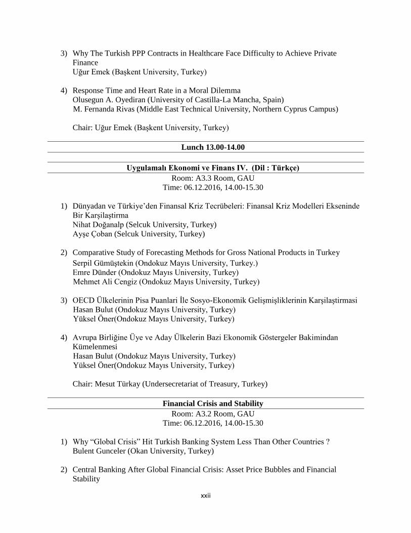
3) Why The Turkish PPP Contracts in Healthcare Face Difficulty to Achieve Private

Finance

Uğur Emek (Başkent University, Turkey)

4) Response Time and Heart Rate in a Moral Dilemma

Olusegun A. Oyediran (University of Castilla-La Mancha, Spain)

M. Fernanda Rivas (Middle East Technical University, Northern Cyprus Campus)

Chair: Uğur Emek (Başkent University, Turkey)

Lunch 13.00-14.00

Uygulamalı Ekonomi ve Finans IV. (Dil : Türkçe)


Time: 06.12.2016, 14.00-15.30

1) Dünyadan ve Türkiye’den Finansal Kriz Tecrübeleri: Finansal Kriz Modelleri Ekseninde

Bir Karşilaştirma

Nihat Doğanalp (Selcuk University, Turkey)

Ayşe Çoban (Selcuk University, Turkey)

2) Comparative Study of Forecasting Methods for Gross National Products in Turkey

Serpil Gümüştekin (Ondokuz Mayıs University, Turkey.)



3) OECD Ülkelerinin Pisa Puanlari İle Sosyo-Ekonomik Gelişmişliklerinin Karşilaştirmasi

Hasan Bulut (Ondokuz Mayıs University, Turkey)

Yüksel Öner(Ondokuz Mayıs University, Turkey)

4) Avrupa Birliğine Üye ve Aday Ülkelerin Bazi Ekonomik Göstergeler Bakimindan

Kümelenmesi


Yüksel Öner(Ondokuz Mayıs University, Turkey)

Chair: Mesut Türkay (Undersecretariat of Treasury, Turkey)

Financial Crisis and Stability


Time: 06.12.2016, 14.00-15.30

1) Why “Global Crisis” Hit Turkish Banking System Less Than Other Countries ?

Bulent Gunceler (Okan University, Turkey)

2) Central Banking After Global Financial Crisis: Asset Price Bubbles and Financial

Stability

xxiii

Abdullah Erkul (Balıkesir University, Turkey)

Tunç Siper (Balıkesir University, Turkey)

3) What is the Real Reason of the Propogation of Financial Crises and How it can be

Stopped?

Dogus Emin (Social Sciences University of Ankara, Turkey)

4) The Effect on Macro Economic Indicators of the Financial Crisis as a Paradox of

Neoliberalism: The Case Of TRNC

Orhan Çoban, (Selçuk University, Turkey)

Nihat Doğanalp, (Selçuk University, Turkey)

Chair: Ilhan Bora (Girne American University, North Cyprus)

Education Economics and Labor Markets


Time: 06.12.2016, 14.00-15.30

1) The Relationship Between Education and Economic Growth in Turkey

Behiye Çavuşoğlu (Near East University, North Cyprus)

2) Education Level and Economic Growth: The European Experience

Mohammad Rajabi (Eastern Mediterranean University, North Cyprus)

Mohammadreza Allahverdian (Eastern Mediterranean University, North Cyprus.)

Mohsen Mortazavi (Eastern Mediterranean University, North Cyprus.)

3) Obstacles Immigrants Faced in Integration to Labor Market: The Sample of Syrian

Immigrants in Turkey

Sefa Çetin (Kastamonu University Turkey)

Hasan Hüseyin Büyükbayraktar (Selcuk University, Turkey)

Abdullah Yilmaz (Selcuk University, Turkey)

4) Female Labor Force Participation Problems in Turkey: Causes and Policy Implications


5) The Impact of Syrian Refugee Crisis on Turkish Labour Market

Aliya Işıksal (Girne American University, North Cyprus)

Dilber Çağlar (Girne American University, North Cyprus)

Yossi Apeji (Girne American University, North Cyprus)

Chair: Feyza Bhatti (Girne American University, North Cyprus)

Applied Banking


Time: 06.12.2016, 14.00-15.30

http://mideast.unc.edu/social-sciences-university-of-ankara-turkey-assistant-professor-of-social-sciences/

xxiv

1) Catering Incentives and Dividend Policy: Evidence from Turkey

Sefa Takmaz, (Adnan Menderes University, Turkey)

2) Determinants of Non-Performing Loans in Central and Eastern European Countries

Ali Özarslan (Middle East Technical University, Turkey)

3) European Banks Financial Strength Ratings: Evidence from a Parsimonious Ordered

Logit Model.

Cem Payaslıoğlu (Eastern Mediterranean University, North Cyprus)

Blerta XHAFA (Eastern Mediterranean University, North Cyprus)

4) The Equipment Leasing as an Alternate Funding Model

Murat Gulec (Banking Regulation and Supervision Agency, Turkey)

5) The Determinants of Borrowing Behaviors of Turkish Municipalities

Hakan Yas (Trakya University, Turkey)

Emre Atılgan (Trakya University, Turkey)

Chair: Cem Payaslıoğlu (Eastern Mediterranean University, North Cyprus)

Applied Banking II


Time: 06.12.2016, 14.00-15.30

1) Distinguishing the Effects of Household and Firm Credit on Income Inequality

Ünal Seven (Central Bank of the Republic of Turkey, Turkey)

Dilara Kılınç (Izmir University of Economics, Turkey)

Yener Coşkun (Capital Markets Board of Turkey, Turkey)

2) The Effect of Foreign Bank Entry on the Financial Performance of the Commercial

Banks in Turkey

Ayhan Kapusuzoglu (Yildirim Beyazit University, Turkey)

Nildag Basak Ceylan (Yildirim Beyazit University, Turkey)

3) Corporate Governance and Financial Constraints

Erkan Solan (Undersecretariat of Treasury, Turkey)

Cumhur Çiçekçi (Undersecretariat of Treasury, Turkey)

4) An Analysis of the Non-Performing Loans of Commercial Banks in Kazakhstan

Hatice Jenkins (Eastern Mediterranean University, North Cyprus)

Zhaneta Kassymbekova (Eastern Mediterranean University, North Cyprus)

Chair: Yener Coşkun (Capital Markets of Turkey, Turkey)


xxv

Multidisciplinary III


Time: 06.12.2016, 16.00-17.30

1) The Tourism Sector in Montenegro in the Context of European Integration.

Radosław Dziuba (University Of Lodz, Poland)

2) Impact of Gold Price And Exchange Rate on Immovable Property Index: Empirical

Evidence From Turkey

Dervis Kirikkaleli, (Girne American University, North Cyprus)

Seyed Alireza Athari, (Girne American University, North Cyprus)

Ilhan Bora (Girne American University, North Cyprus)

Hasan Murat Ertugrul (Girne American University, North Cyprus)

3) Effect of Islamic Banking on Employment in Punjab, Pakistan

Bilal Ashraf (University of Gujrat (Punjab), Pakistan)

4) The Dual Adjustment Approach with Popular Filters

Mustafa Ismihan (Atilim University, Turkey)

Mustafa Can Küçüker(Atilim University, Turkey)

5) Does Unemployment Rate Have a Unit Root

Mustafa Ismihan (Atilim University, Turkey)

Chair: Seyed Alireza Athari, (Girne American University, North Cyprus)

Uygulamalı Ekonomi ve Finans V. (Dil : Türkçe)


Time: 06.12.2016, 16.00-17.30

1) An Application Of Panel Data Analysis For Export In Turkey




2) Efficiency Assessment Of The Transportation Services In Turkey

Serpil Gümüştekin (Ondokuz Mayıs University, Turkey)

Talat Senel

3) Politika-Ekonomi İlişkileri Üzerine Teorik Yaklaşımlar: Politik Konjonktür Teorileri

Sema Yilmaz Genç (Kocaeli University, Turkey)

Duygu Süloğlu (Kocaeli University, Turkey)

4) Yaşayan Efsane Beetle’nin Türkiye Piyasa Fiyatinin Modellenmesi


xxvi

Tolga Zaman (Ondokuz Mayıs University, Turkey)

Ebrucan İslamoğlu (Nevşehir Hacı Bektaş Veli University, Turkey)

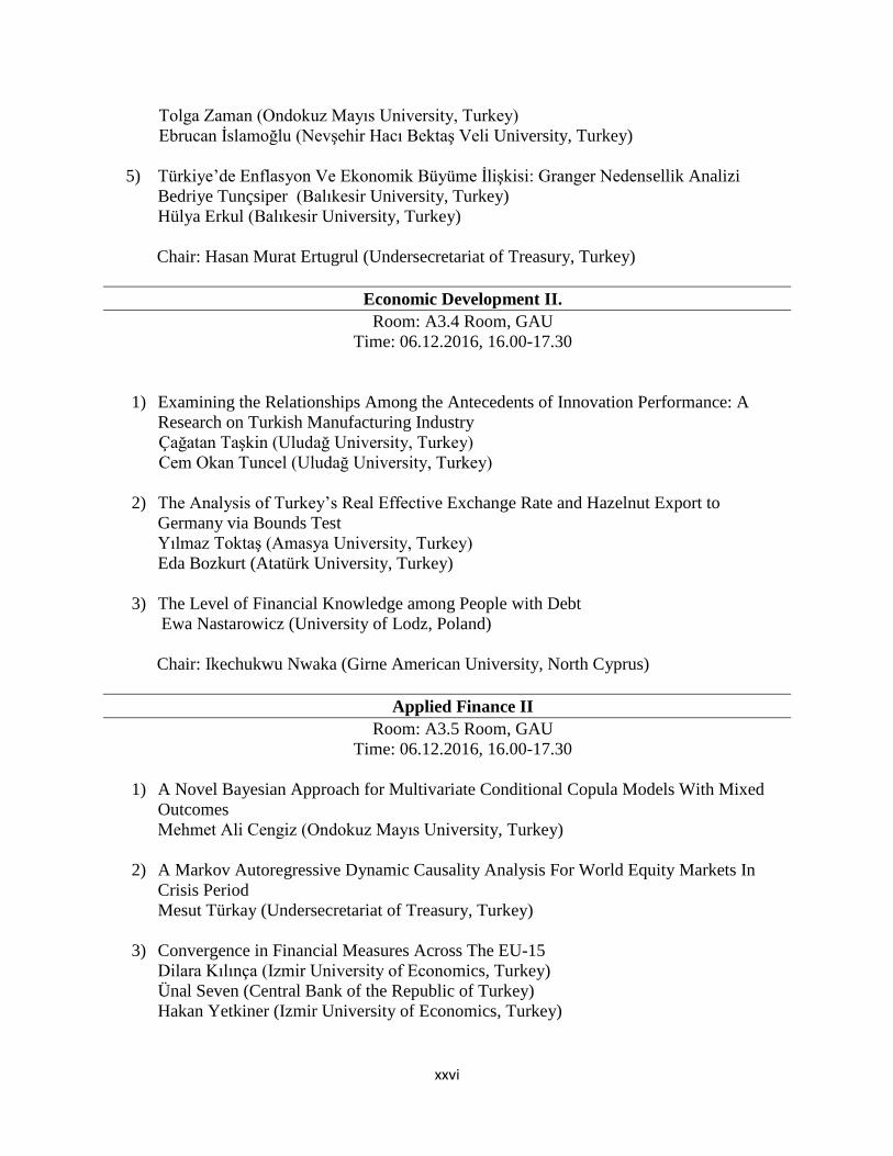
5) Türkiye’de Enflasyon Ve Ekonomik Büyüme İlişkisi: Granger Nedensellik Analizi

Bedriye Tunçsiper (Balıkesir University, Turkey)

Hülya Erkul (Balıkesir University, Turkey)

Chair: Hasan Murat Ertugrul (Undersecretariat of Treasury, Turkey)

Economic Development II.


Time: 06.12.2016, 16.00-17.30

1) Examining the Relationships Among the Antecedents of Innovation Performance: A

Research on Turkish Manufacturing Industry

Çağatan Taşkin (Uludağ University, Turkey)

Cem Okan Tuncel (Uludağ University, Turkey)

2) The Analysis of Turkey’s Real Effective Exchange Rate and Hazelnut Export to

Germany via Bounds Test

Yılmaz Toktaş (Amasya University, Turkey)

Eda Bozkurt (Atatürk University, Turkey)

3) The Level of Financial Knowledge among People with Debt

Ewa Nastarowicz (University of Lodz, Poland)

Chair: Ikechukwu Nwaka (Girne American University, North Cyprus)

Applied Finance II


Time: 06.12.2016, 16.00-17.30

1) A Novel Bayesian Approach for Multivariate Conditional Copula Models With Mixed

Outcomes


2) A Markov Autoregressive Dynamic Causality Analysis For World Equity Markets In

Crisis Period

Mesut Türkay (Undersecretariat of Treasury, Turkey)

3) Convergence in Financial Measures Across The EU-15

Dilara Kılınça (Izmir University of Economics, Turkey)

Ünal Seven (Central Bank of the Republic of Turkey)

Hakan Yetkiner (Izmir University of Economics, Turkey)

xxvii

4) Measuring the Financial Contagion: Evidence from Dynamic Betas and Similarity Based

Network Structure

Burak Sencer Atasoy (Undersecretariat of Treasury, Turkey)

Onur Polat (Illinois State University, USA)

İbrahim Özkan (Hacettepe University, Turkey)

5) The Relationship between Elements of Internal Financial Flexibility in Market

Participant`s Decision Making

Parviz Piri (Urmia University, Iran)

Samaneh Barzegari Sadaghiani (Urmia University, Iran)

Fariba Abeli Habashi (Urmia Azad University, Iran)

Chair: Ünal Seven (Central Bank of the Republic of Turkey)

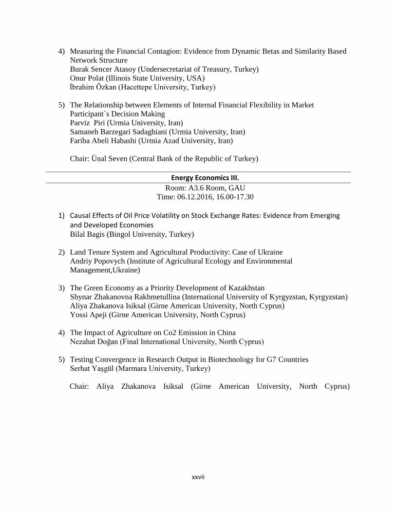
Energy Economics III.


Time: 06.12.2016, 16.00-17.30

1) Causal Effects of Oil Price Volatility on Stock Exchange Rates: Evidence from Emerging

and Developed Economies Bilal Bagis (Bingol University, Turkey)

2) Land Tenure System and Agricultural Productivity: Case of Ukraine

Andriy Popovych (Institute of Agricultural Ecology and Environmental

Management,Ukraine)

3) The Green Economy as a Priority Development of Kazakhstan

Shynar Zhakanovna Rakhmetullina (International University of Kyrgyzstan, Kyrgyzstan)

Aliya Zhakanova Isiksal (Girne American University, North Cyprus)

Yossi Apeji (Girne American University, North Cyprus)

4) The Impact of Agriculture on Co2 Emission in China

Nezahat Doğan (Final International University, North Cyprus)

5) Testing Convergence in Research Output in Biotechnology for G7 Countries

Serhat Yaşgül (Marmara University, Turkey)

Chair: Aliya Zhakanova Isiksal (Girne American University, North Cyprus)

28

FULL PAPERS

CONTRADICTIONS IN PUBLIC-PRIVATE PARTNERSHIP DEVELOPMENT

WITHIN TRANSITIONAL ECONOMIES

Alla Mostepaniuk


Email: [email protected]

Abstract

The paper is devoted to the study of the public-private partnership (PPP) development

process within transitional and advanced economies. Based on successful practice of PPP

projects in advanced countries, implementation of appropriate practical steps to expand PPP

practice in transitional economies was provided. Moreover, the key contradictions of PPP

development within transitional economies were identified as well as the methods to solve or

minimize them. The main channels of financial investments in infrastructure of transitional

economies and the distribution of investments within sectors of infrastructure were analysed.

The empirical analysis has shown the impact of economic freedom and the living standards

levels on private investments (domestic and foreign) in infrastructure projects within

transitional economies.

Keywords: Transitional economy, public-private partnership (PPP), PPP projects,

contradictions of PPP, infrastructure.

Introduction

Transitional economy is characterized by temporal interrelated changes from traditional

inefficient economic system to modern one, for transitional economies in Central and East

Europe the movement is from the command state system to the free market economy.

Throughout transforming an economy is unstable and sometimes even has chaos features, as

elements of previous system are transforming to the new kind; meanwhile the state lowers its

power and even can lose the control of some areas of economic system. Besides that the key

transitional processes are aimed at specifically institutional and legal reforms that leave out of

date objects of infrastructure still existing in transitional economies. Under those conditions

the private business is playing its crucial role as a mechanism to stabilize the economic

environment in a form of taking or sharing government’s social functions in the time of

transition, when the pressure on the budget is heavy and there is some uncertainty.

Literature review

Key determinants of PPP development

Kasri and Wibowo (2015) in their study presented the empirical evidences that prove the

main determinants of PPP implementation, the first is the market conditions – the higher the

demand for public services is the more attractive sector is for private investors, the second is

institutional quality and effective government – the better legal and state protection is

provided to investors the higher their investments are. At the same time the paper, based on

the empirical data, disapproves some determinants such as macroeconomic conditions and

budget constraints.


29

Mozsoro and Gasiorowski (2008) designed the model-based analysis, which showed that PPP

projects may provide public services cheaper than a sole private or sole public entity. They

underlined that PPP projects are more efficient in 1) stability-oriented government policy

countries, where for private sector cheaper financing conditions are available and

encouraging by the state; 2) countries with a reliable legal system that provides the

instruments to protect the interest of the public partner and the private partner. The key

barriers were proven such as: a lack of trust and confidence between the partners, an

insufficient legal framework, and the unstable macroeconomic policies, that prevent private

partner of cooperation with the state.

PPP in transitional economies

Yang Y. et al. (2013) designed Theoretical Framework of PPP development in transitional

economies, which contains tree pillars: Government (government actions), Market (financial

environment) and Operating Environment (government and legal regulations). Moreover,

based on mentioned Framework and major barriers seven crucial factors that enable PPP

development in transition economies were identified, such as: market potential, institutional

guarantee, government credibility, financial accessibility, government capacity, consolidated

management and corruption control. Based on their research, contradictory conclusions were

conducted, meaning, PPPs in transitional economies have some advantages comparing to

advanced ones: transitional economies have greater business potential for PPP (more

profitable than in advanced countries) and at the same time greater institutional and legal

risks; the movement from centralized to market economy simplifies procedures and

regulations comparing to advanced economies with highly complex legal regulations on PPP.

Zagozdzon (2013) investigated the specifics of PPP implementation in transition economies

based on Polish case; the author described a PPP market in transition countries as “an under

construction market” and suggested the following factors as crucial to succeed in PPP: 1) the

government’s economic policy regarding privatization and deregulation, 2) the level of

financial market development and strict financial policy, 3) the competition in the public

procurement market, 4) adapted legal system to the specifies of PPP projects, 5) the

government PPP-oriented policy, supporting and promoting partnership projects.

Sharma (2012) provided the first attempt to identify the determinants of PPP in developing

countries; this empirical study evidenced the following key determinants: macroeconomic

conditions, market size, quality of regulation and governance, at the same time the

importance of political factors and budget constraint was not proven.

Urio (2007) in the research paper identified key determinants of PPP projects in transition

economies and the crucial dilemma for a government. First of all, talking about determinants

of PPP projects the author highlighted the concept that to “copy” current legal rules and

regulation on PPP is not the efficient method to develop PPP as it means to use the identical

“surface” without required fundamentals. The second significant impact of the paper is on a

government’s dilemma as a government generally aims at three goals: to maintain its control

on public services sector and to improve the quality of public services and to allocate

efficiently available resources, but while using PPP as a mechanism to attract private

investments and to improve the quality of public sector without or with lower costs from the

budget the state is losing its monopolistic power. According to the authors, the state should

follow the PPP principles as long as it faces the risk for autonomous development or national

independence.

30

Benefits and risks in PPP implementations in transitional economies

Kripa (2013) made a research on benefits and risks of PPP projects for each economic actor:

a private sector, a government and society. According to the paper a government will use PPP

as a mechanism to relocate the budget money, using private investments and their fees where

it is possible and saved budget funds, in that case, can be invested in another sector, at the

same time, a government will lose its power in previous monopolies; while implementing

PPP projects a government will face possibility that a project will be cancelled at all.

Business will benefit also in a way that some state monopolies will be available for investing,

private sector will obtain the opportunity to improve and innovate their activities, to become

more competitive comparing to other firms, of course as a result of PPP contract business will

have some restrictions mostly connected to the state’s price policy in order to protect

consumers and to hold prices at the same affordable level. Finally, society will also benefit

because of the new innovative methods of providing public services, better quality and

variety of services, but talking about risks, specifically in transitional economies, as

consulting processes are not holding “transparently”, that’s why the society’s interests are not

always included in the PPP projects, rather business’ and government’s interests.

Harris and Pratap (2009) studied reasons of cancelling PPP projects and identified the most

crucial ones that make higher probability of cancelling the project as following:

macroeconomic shocks most probably increase the cost of project financing for a foreign

investor (exchange rate depreciation) or through increases in domestic interest rates for a

local investors; the presence of a foreign sponsor; the size of the project, the bigger project

the higher financial burdens are imposed on the government; the level of government that

provides PPP projects, PPPs established by local governments have lower probability to be

cancelled than by other levels. Moreover, the study shows that institutional quality has no

significant impact on cancellation and control of corruption has significant impact on

reducing the probability of cancelling the project.

Andres et al. (2008) provided a study based on developing countries (specifically on Latin

American countries) that shows that infrastructure facilities after changing in ownership from

public to private started to perform more efficient; first of all it was seen in higher labor

productivity, improvement in distribution losses and better quality of services. According to

the paper the key deficiencies for private partner are as following: the lack of motivation, the

absence of social programs aimed at supporting and protecting PPP projects, the absence of

transparency in financial actions, weak legal framework and contract violations.

Corrigan et al. (2005) in their paper “Ten Principles for Successful Public/Private

Partnerships” identified key risks and rewards for public and private partners. Public sector

within PPP projects is challenged by conflicts of interests, misusing of public funds and

resources, a developer failure to implement PPP projects, public opposition, at the same time

some rewards will become available for public as: better infrastructure, job creation, an

increase in quality of life, greater community wealth, advance city image. The other partner,

private business, will face some specific risks: increasing costs of PPP implementation, time-

consuming process of PPP, failures to complete projects, a change in key public and/or

political leaders, market failures; private sector will obtain some benefits namely: new

resources to sustain organization, higher profitability, value/wealth creation, community

support, better image, reputation and experience to get next projects.

31

Latest scientific literature reasonable have defined the key determinants of successful PPP

projects implementation and factors that can cause their delaying or sometimes even

cancellation both in transitional and advanced economies. As it was mentioned above while

implementing PPP projects the conflict of interests occurs, especially because of the opposite

motives from the state and business. The issue of public and private motives and benefits

needs to be studied better in the context of comparison the PPP principles in advanced and


The purpose of the paper is to provide a comparison analysis of PPP principles in advanced

and transitional economies, to determine the characteristics and contradictions of the

formation of partnerships between government and business in transition economies, to

identify the impact of the developing stage of a country on its values of PPP practice and to

develop on this basis practical recommendations for improving the mechanisms of PPP

implementation.

The current scientific literature analysis shows that a transition economy is defined as a

special phase of economic system development through moving from “old” to “new”

economic system (from traditional to modern) following by evolutionary and/or revolutionary

qualitative changes. Such changes related to all elements of the economic system, starting

from methods of resources allocation, property rights, methods of production, models of

labor motivation, objectives and factors of socio-economic development, to institutional

environment (Grazhevska, 2008).

In the late twentieth century about thirty former socialist countries abandoned the command-

administrative economic system and made deep institutional changes aimed at building a

market economy. According to researchers, these countries were trapped into a situation of

so-called "triple transition": to the market system, democratic political institutions, as well as

integration into the global market. Mentioned above created the new model of "transition

state” and intensified the necessity to increase the “role” of the state in order to overcome the

weakness of the national business and form civil society (Haggard, 1995; Howard, 2002).

The transformation processes in different countries have certain specific characteristics;

however, it’s possible to identify key common features inherent to transition economies:

1. systematic character of changes as all elements of the existing structure have to be

replaced;

2. marginal imbalance and instability associated with temporary elements domination

(alternative structures and organizations), parallel structural elements;

3. abnormality, crisis and conflicts domination, resulting from public and business

interests disparity and leading to social conflicts aggravation, chaotic changes in the

normative-value system of society;

4. normative imbalance that occurs as a result of institutional changes when informal

interactions replace formal rules, the transition from explicit to implicit contracts, from

standardized to customized, sometimes even double standards, local institutions and so on.

5. multi-structure that occurs under coexistence and combating existing and new socio-

economic elements and structures;

6. alternative confrontation of old and new forms of economic activity, and their

coexistence as a result of economic systems inertia;

7. contradictory and alternatively social-economic and political development

(Bazylevych, 2004; Grazhevska, 2007).

32

Generally, transition economies are characterized by its abnormal and unstable process of

development as old elements are “dying” and their roles are putting on completely new

elements.

In the purpose of the study its worth to mention about the continuity of socio-economic

transformation, that makes it difficult to determine the completion of the transition from the

old economy to a new quality. That is why the World Bank defined the ultimate goal of

transition for the 28 countries that have transformed towards establishing a market economy

in 1996 and suggested the following four criteria for assessing the progress of socio-

economic transformation: 1) liberalization of the economy; 2) development of property

rights; 3) development of new relevant institutions; 4) social orientation of public policy

(Jahan, 2015).

Based on current literature the key contradictions of PPP development in transitional

economies are defined as: 1) the growth of social stratification caused by different access to

strategic resources; 2) the formation of elitism as the organizing principle of economic

activity as parallel with moving from command to market economy old norms are getting

weaker and new one is only forming, under such uncertainty the role of elite groups are

getting more powerful, meaning that they form the ruling group; 3) the weakening of

democratic structures and civil society caused by chaotic features of transitional economy; 4)

the emergence of the phenomenon like "digital inequality" and " computer exclusion"; 5) the

development of "PR" and the spread of technology "brainwashing"; 6) the aggravation of

global issues as the mail goal for transitional economies is to build new economic and legal

framework but not do deal with current issues, etc. (Bazylevych, 2004; Grazhevska, 2007;

Howard, 2002).

Resolving these contradictions requires strengthening the state’s role and establishing of

reliable partnerships between key economic actors (government and business) to reform all

public sector elements. General flows of modern-day economic development such as post

industrialization and globalization of the economy should be taken into account; mentioned

involve a movement from a simple reproductive strategy to innovative, meaning that the

government policy is aimed at stimulating innovative economic activities (Figure 1).

33

Figure 1. State’s role in transition economies.

Source: based on (Bordoev, 2008).

During the process of institutional transformation, moving from old norms to new, their

power and reliability declined at the same time instability and uncertainty appeared. Under

those conditions public-private partnership became an important mechanism to balance and

promote equality between private and state interests. Talking about PPP development in

transition economies it needed to be mentioned that contradictions mostly appeared between

“privatized” state and society, as “big” business sector privatized state property using “grey”

gaps in the law (Heyets, 2009). All characteristics of transition economy have their influence

on the practice of PPP projects implementation, distinguishing feature of PPP in market and

transition economy are presented in the table 1.

State’s role in transitional economies

The choice of national development

priorities, particularly in high-tech and knowledge-

intensive sectors.

The balance of public and private investments

in R&D and formation of public-private

partnerships on this basis.

The creation of the new national innovation

system structure using clusters, technology parks

and research centers.

Encouraging universities to shift from the classical

scheme "science + education" to the scheme

"Science + Education + Innovation Business".

The improvement of the institutional

framework of the new economy associated with the

use of intellectual property.

34

Table 1. Distinguishing features of public-private partnerships in advanced and


№ Advanced economies Transitional economies

1

.

PPP subjects are business and

representatives of the state, isolated from big

business

Subjects PPPs are representatives of

state and business who have influence on

public authorities

2

.

The ”transparent” procedure of

competition to determine the private partner

The “not transparent” competition to

determine the private partner

3

.

Developed regulatory framework

regulation of cooperation between state and

business

Imperfect legal framework regulating

the processes of cooperation between state

and business

4

.

Rational choosing a business partner Significant influence of future personal

benefits on the choice of business partner

5

.

The interest of private businesses in

their own profits and social benefits as a

result of improving public sector

The interest of private business

exclusively in their own financial gain

6

.

Encouragement, support and guarantee

to business from the government

Lack of motivation of the private sector

to cooperate with the state

7

.

Developed methodologies for public-

private partnerships accounting and

efficiency evaluation

There are no or only developing

methods of accounting and evaluation of

public-private partnerships

8

.

The main purpose of cooperation

between the state and business is the

improvement of state property at the

expense of private investment

The main purpose of cooperation

between the state and business is the

"capture" of state property by private

businesses for further financial gain

9

.

State and business are equal partners The state has a greater impact than

private business

1

0.

Trust between government and business

supported by current laws

Lack of trust between government and

business

1

1.

The PPP procedures and practiced were

developed gradually based on current needs

and goals.

The PPP procedures and practiced were

“copied” directly from advanced countries

without any adjusting them to the country’s

current needs and goals.

Source: designed by the author

Thus, in the process of economy’s transformation the principles of cooperation between the

state and business representatives deformed, that caused by the imperfection of the existing

institutional framework, changing the practice of interactions from competing to cooperative,

shifting the goals from financially to socially beneficial. The purpose of such a partnership

has to be taken into account: in a market economy – the development of PPP is for more

complete satisfaction of public needs, in a transition economy – mostly to meet the needs of

private business by providing opportunities to obtain regular income.

The potentially more profitable sectors of infrastructure attract higher financial investments,

as a private partner has two complement issues to invest rationally and to support the state

partner in providing and maintaining the public infrastructure objects. Talking about the

financial inflows in infrastructure it has to be mentioned the rest factors that influence on the

investments behaviour such as: the general image of a country on the global level, the level of

35

openness of going business, the level of reliability to the legal system, the level of social

acceptance of a business as a provider of public goods, the level of trust between the state and

private partner, the level of transparency of competition within a country, the wiliness to

adapt new global trends as PPP etc.

The World Bank database on Private Participation in Infrastructure allows us to study the

distribution of private incentives on PPP among core sectors: water and sewerage,

telecommunication, roads and ports, natural gas, electricity.

Figure 2. Distribution of PPP projects within public sectors in transitional countries

(2000-2015 years, USD million).

Source: Private Participation in Infrastructure Database, 2015.

For the research we use such transitional economies as Lithuania, Russian Federation,

Romania, Bulgaria, Belarus, Bosnia and Herzegovina and Ukraine (the figure above), based

on the data we can conduct that there is a “common pattern” of PPP projects distribution in

infrastructure sectors: the most valued sectors are telecommunication and energy providing

sectors as natural gas and electricity for transitional economies. The sectors, were PPP

projects were implemented successfully, indicate the spheres where the “importance” and

“necessity” to be improved for public were accompanied with the private incentives. To find

the projects that will be attractive and profitable for private partner and appreciated by the

society and beneficial for the state is the first step to support and develop the PPP practice as

a mechanism of reducing financial pressure on the state and at the same time improving the

living conditions to society.

Our analysis shows that mostly governmental financial expenditures connected to

maintaining the public sphere (particularly infrastructure objects) in transitional economies

replaced or shared with private business, more specifically foreign private investors. The data

on private investments in infrastructure (the table below) provides the picture on current

investment flows in transitional economies, the biggest financial flows are coming from the

local businesses (around 70% of total investments in infrastructure), than from Russian

36

Federation (around 20%), the following countries are advanced countries with small shares

such as Germany (about 4%), Norway (1.5%), Sweden (1.5%), Austria (around 1%) etc.

Table 2. The main sources of private investments in infrastructure (2000-2015

years, USD million)

Lit

hu

ania

Russ

ian

Fed

erat

ion

Rom

ania

Bulg

aria

Bel

arus

Bosn

ia

and

Her

zegovin

a

Ukra

ine

Tota

l

Domestic 63315 532 351710

Russian

Federation 464 3064 108010 111538

Germany 209 23246 351 18 23824

Norway 7054 1742 8796

Sweden 1581 6782 164 8527

Austria 354 2595 1581 1095 5625

Greece 4652 4652

United States 4282 4282

France 3792 130 3922

United Kingdom 339 2364 662 3365

Czech 1619 1449 3068

Italy 2323 2323

Turkey 1011 882 1893

Serbia 789 789

Portugal 371 371

China 248 248

Estonia 130 130

Bulgaria 47 47

Netherlands 33 33

Slovenia 25 25

Cyprus 4

4


Noteworthy to mention the reasons of such distribution: first of all, as it was discussed

previously by researchers, the low rates of return on infrastructure projects, that makes them

“not attractive” to foreign investors, the second reason is that local business are more

motivated to invest in socially beneficial projects rather than foreign companies, the third

reason is the lower possibility of projects cancellation when local business invest compared

with external sources of financing, the forth reason is the level of economic freedom and the

easiness of doing business, the fifth one is the stage of economic development of a particular

country. The impact of the last two factors will be discussed later.

37

Figure 3. The relationship between total private investments in infrastructure (2000-

2015, USD million) and the Gross national income per capita (current USD)


The figure above presents the relationship between the total private investments in

infrastructure in transitional economies from 2000 to 2015 in USD million and the Gross

National Income per capita in current USD; this analysis shows the impact of economic

developing meaning improving leaving standards on PPP development measured in total

private financial flows to public sector.

There are two hypotheses: 1) with an increase in GNI per capita the living standards will be

improved, that means that lower will be the “need” to attract private investments to develop

public sectors, which supports the negative correlation; 2) when the GNI per capita increases

the county’s image becomes more reliable that attracts domestic and foreign private financial

inflows, that means that there is a positive correlation. The data and graph above support the

second hypotheses and show that there is a positive relationship between GNI per capita and

PPP development.

To study the impact of the Index of economic freedom we present the graph below, that

proves that as more “transpared” and “open” country is the higher values of domestic and

external private investments in infrastructure in transitional economies are, it means that

positive correlation exixts.

38

Figure 4. The relationship between total private investments in infrastructure

(2000-2015, USD million) and the index of economic freedom (2015).


The index of economic freedom shows how the state control or influence on the business

activities, this measure is important as the state is the equal partner in PPP that assumes that

the state partner will not use its pover agains the private partner or in order to sutisfy only

their own interests, that can help to implement mutually beneficial projects of private-public

cooperation. The state’s power in transitional economies is relativety high comparing to

advanced as the system is moving from the command regulation to free market; besides that

satate policy is still unstable and unpredictable because of transitional changes, that makes all

business activities as separetly and jointly with the state sector risky.

Table 3. Pearson correlation test results (SPSS software used)

Correlations

TI ECFR GNI

Pearson

Correlation

TI 1,000 -,346 ,324

ECFR -,346 1,000 ,634

GNI ,324 ,634 1,000


Finally, the Pearson corellation test was used to find the significance of the factors impact on

total private investments in infrastructure (in transitional economies), the results are presented

in the table 3. The first correlation to study was between total private investments in

infrastructure (TI) and the Index of economic freedom (ECFR), Pearson colletion test shows

39

the negative moderate relationship (-0.346), the second is on TI and gross national income

per capita (GNI), the test shows the positive moderate relationship (0.324), the third is on

ECFR and GNI, the test shows the strong positive relationship (0.634).

Conclusions

1. Distinguishing features of public-private partnerships in advanced and transitional

economies are defined, the most significant contradictions of transitional economies are:

-state officials own business that can be seen as a “potential” private partner for

implementation the PPP projects and can use their influence on the decisions, it makes

impossible to provide “transparent” competition to choice the private partner;

- the main purpose of cooperation between the state and business is the "capture" of

state property by private businesses for further financial gain rather than to improve the

public sector and to share the government’s financial pressure;

- lack of public trust to government and business caused by previous “personally

efficient” but not “socially efficient” projects, practice of using personal channels and

connections in rent seeking that decreases the country’s efficiency, causes inefficient

allocation of available resources and sometimes even some decrease in the government’s

revenue;

- imperfect and sometimes “copied” from the advanced countries legal framework

contains “grey gaps”, the weak places in the norms and regulations that allow officials and

businesses to use it in order to reach their personal financial goals.

2. The specifics of transformational economy highly modify the social values and

procedures of implementation of PPP projects; it is connected with the use of both formal and

informal mechanisms, lack of transparency caused by driving competitions, abuse and

corruption of the authorities, at the same time, by the unfair competition of private business.

3. Based on such transitional economies as Lithuania, Russian Federation, Romania,

Bulgaria, Belarus, Bosnia and Herzegovina and Ukraine we can conduct that there is a

“common” pattern of PPP projects distribution in infrastructure sectors: the most valuable

sectors are telecommunication and energy providing sectors as natural gas and electricity.

The sectors, were PPP projects were implemented successfully, indicate the spheres where

the “importance” and “necessity” to be improved for public were accompanied with the

private incentives.

4. The data on private investments in infrastructure in transitional economies shows

that the biggest financial flows are coming from the local businesses (around 70% of total

investments in infrastructure), than from Russian Federation (around 20%), the following

countries are advanced countries with small shares such as Germany (about 4%), Norway

(1.5%), Sweden (1.5%), Austria (around 1%) etc. Factors that influence are: the low rates of

return on infrastructure projects, that makes them “not attractive” to foreign investors; local

business are more motivated to invest in socially beneficial projects rather than foreign

companies; the lower possibility of projects cancellation when local business invest

compared with external sources of financing; the level of economic freedom, the easiness of

doing business; the stage of economic development of a particular country.

5. The study supports that when the GNI increases that builds up a county’s image

and attracts as domestic as foreign investors, which means that there is a positive correlation

exists.

6. To paper proves that as more “transpared” and “open” country is the higher values

of domestic and external private investments in infrastructure in transitional economies, it

means that positive correlation exixts.

7. Pearson corellation test shows the negative moderate relationship (-0.346) bettwen

total private investments in infrastructure and the Index of economic freedom; the positive

40

moderate relationship (0.324) bettwen total private investments in infrastructure and gross

national income per capita; the test shows the strong positive relationship (0.634) between the

Index of economic freedom and gross national income per capita.

Recommendations:

The research shows the directions for further PPP development in transitional economies:

1. To buil up and develop an appropriate legal system for suppotring and controlling

PPP projects in accordance to the current needs of each particular transitional country.

2. To separate the represantatives of the state and big businesses using legal regulation

in order to provide “transparent” procedures of choicing the priorities that are required by the

society not by the business only and selecting the private partner that can “objectively”

perform better not just becouse of their connections.

3. To provide clear and easy entry of foreign investors in order to support and develop

further the PPP practice in transitional economies as investors from advanced countries can

share their previous experiences and even prevent some financial risks.

4. To create conditions for attracting highly qualified specialists to develop and

implement efficient infrastructure projects based on public-private partnerships in order to

build trustful relations between the state, private business and society;

5. To work on factors that support the process of PPP developments as economic

stability, social acceptance of PPP practice, state policy orientation on socially efficient

projects, government’s guarantee to business in PPP projects, smart adoptation of advanced

countries policies etc.

References

1. Andres, L. A. et al. (2008). The Impact of Private Sector Participation in

Infrastructure: Lights, Shadows, and the Road Ahead. doi: 10.1596/978-0-8213-7409-

2

2. Bazylevych, V. D. (2004). Formation of the competitive environment in transitive

economy: challenges, trends and contradictions. Competition, 2, 24-28.

3. Bordoev, D. G. (2008). Government Regulation of the Russian Economy in the Post-

industrial Transformation. Saint Petersburg.

4. Corrigan, M. B. et al. (2005). Ten Principles for Successful Public/Private

Partnerships. Washington, D.C.: ULI–the Urban Land Institute.

5. Grazhevska, N. I. (2007). Display of transformation processes in the system of social

and economic dynamics categories. Economic theory, 4, 19-29.

6. Grazhevska, N. I. (2008). The Economic System of the Era of Global Changes. Kyiv:

Znannya.

7. Haggard, St. et al. (1995). The Political Economy of Democratic Transitions.

Princeton: Princeton University Press.

8. Harris, C. G., Pratap, K. V. (2009). What drives private sector exit from

infrastructure? Economic crises and other factors in the cancellation of private

infrastructure projects in developing countries. Gridlines, 46. Washington, DC: World

Bank.

9. Heyets, V. M. (2009). Society, State, Economy: Phenomenology of Cooperation and

Development. Kyiv: Institute of Economics and Forecasting.

10. Howard, M. M. (2002). The Weakness of Postcommunist Civil Society. Journal of

Democracy, 13(1), 157-169.

11. Jahan, S. (2015). Global 2015 Human Development Reports. Retrieved from

http://hdr.undp.org/sites/default/files/2015_human_development_report.pdf

http://hdr.undp.org/sites/default/files/2015_human_development_report.pdf

41

12. Kasri, R. A., Wibowo, F. A. (2015). Determinants of Public-Private Partnerships in

Infrastructure Provision: Evidence from Muslim Developing Countries. Journal of

Economic Cooperation and Development, 36, 1-34.

13. Kripa, E. (2013). Role of Public Private Partnership in Infrastructure Development.

Advanced Research in Scientific Areas, 2(6), 209-214.

14. Mozsoro, M., Gasiorowski, P. (2008). Optimal Capital Structure of Public-Private

Partnerships. Retrieved from

https://www.imf.org/external/pubs/ft/wp/2008/wp0801.pdf

15. Sharma, Ch. (2012). Determinants of PPP in infrastructure in developing economies.

Transforming Government: People, Process and Policy, 6(2), 149-166. doi:

10.1108/17506161211246908.

16. Private Participation in Infrastructure Database. (2015). Retrieved from

http://ppi.worldbank. org/data

17. Urio, P. (2007). Under What Conditions Can Public-Private-Partnerships (PPPs)

Improve Efficiency, Equity, Security and Sustainable Development in Countries at the

Pre-PPP Stage? Retrieved from

http://science.ksc.nasa.gov/shuttle/nexgen/Nexgen_Downloads/Public_Private_

Partnerships-Urio.pdf

18. Yang, Y. et al. (2013). On the Development of Public–Private Partnerships in

Transitional Economies: An Explanatory Framework. Public Administration Review,

73(2), 301–310. doi: 10.111/j.1540-6210.2012.02672.x

19. Zagozdzon, B. (2013). Determinants of Implementation of Public-Private Partnership

in Poland: the Case of Transport Infrastructure. Advances in Economics and Business,

1(2), 57-71. doi: 10.13189/aeb.2013.010203

42

THE EFFECT OF PROSPERITY ON INTERNATIONAL TOURISM

EXPENDITURES

Amin Sokhanvar Eastern Mediterranean University, North Cyprus


Iman Aghaei Eastern Mediterranean University, North Cyprus

Şule L. Aker Eastern Mediterranean University, North Cyprus

Abstract

This paper implements a 2SLS estimation method with fixed effects specification to study the

prosperity-international tourism expenditures nexus. While studies have focused on the impact of

income on international tourism expenditures, none consider the effect of prosperity on tourism

expenditures. We apply panel regression analysis, using annual panel data for the sample period

between 2009-2013 on 98 countries. The estimation results reveal a statistically significant

relationship between tourism expenditures of the citizens and prosperity, when prosperity is

measured using its sub-indices including Entrepreneurship & Opportunities, Government

Efficiency, Education, Health, Safety & Security, Personal Freedom, Social Capital and Economy

of the country. Education, Safety & Security, and Health are the most significant factors which

affect tourism expenditures of the country of origin. Tourism policy implications are also

discussed.

Keywords: Panel Data, Prosperity, Tourism Expenditure, Entrepreneurship, Economy,

Safety, Health.

1. Introduction

It is necessary to discover the determinants of tourism expenditures since the revenue

obtained from tourism is an important source of income for lots of host countries. Finding

those determinants can provide valuable information for tourism marketing.

Providing insight into the tourism economy details is easier by studying tourism

expenditures. It plays a significant role in studying the impact of travel on economies of

countries. It affects economic development in parallel with changes in consumer

expenditures. Economic benefits of tourism to the host and home countries can be analyzed

by detailed information provided by international tourism expenditures data.

International tourism plays a rising significant economic role in the world. International

tourism expenditures including accommodations, shopping, transportation, food and

beverages, entertainment and sightseeing contributes notably to local economies. It has

improved GDP growth, promoted economic and social development and created job

opportunities. Therefore, researchers have paid a great attention to study tourism

expenditures (Yu Shan Wang,2014).

43

Despite the global economic recession and financial crisis of late 2008 and 2009, the

recovery of international tourism has excelled predictions (United Nations World Tourism

Organization, UNWTO, 2011): The number of international tourists increased from 681

million in 2000 to 939 million in 2010, and 980 million in 2011 because of the increase in

disposable income. International tourism expenditures have also increased in emerging

markets like China, India, Russia and Brazil. According to many articles that have been

published after business cycle 2006-2010 and economic crisis in 2008, the important role of

tourism expenditure in a country’s economic growth became noticeable, as we can find a few

notable articles in favor of this argument in recent years. While global tourism continues its

ascending trend, the benefits of the sector are not the same for all countries with important

tourism sector. So we aim to find the most important factors affecting tourism.

The presumption is that a nation’s tourism expenditure is not solely affected by

macroeconomic indicators such as home country’s income, represented by GDP per capita.

Non-economic factors may also be effective on tourism expenditures. In fact, it can be

affected by not only accumulation of material wealth but also joy of everyday life. Travel

participation is also affected by cultural characteristics of the country of origin. That’s why

we select prosperity index which include both economic and non-economic factors, to study

international tourism expenditure. This Index is the only global measurement of prosperity

based on both wellbeing and income. It is the definitive gauge of global progress and the

most comprehensive indicator of its kind. The Legatum Prosperity Index offers a unique

intuition into how prosperity is reforming and changing across the world.

In contrast to most empirical studies on tourism expenditure in which economic factors are

analyzed, in this study we analyze non-economic determinants of the international tourism

expenditures by exploiting Prosperity Index of the country of origin. In fact, an important

contribution of this paper is the definition and design of variables determining tourism

expenditures.

The aim of this paper is to try to give an answer to the following questions: Did non-

economic factors in the country of origin lead to a change in the tourism industry through

changes in tourism expenditures? Which factors have maximum impact on tourism

expenditures? This study analyzes if there are relationships between international tourism

expenditures and prosperity sub-indices including Entrepreneurship & Opportunities,

Government Efficiency, Education, Health, Safety & Security, Personal Freedom, Social

Capital and Economy across home countries during 2009-2013. It also estimates the

significance and direction of the effects.

Our specifying assumption is that a critical indirect role is played by some non-economic

factors on international tourism expenditures through the direct effect of some transmission

channels which the literature has identified in Economy and Entrepreneurship (in the country

of origin) among the main ones. This assumption allows us to examine the effect of non-

economic factors on their natural economic targets and also to check the side effect played on

tourism industry and tourism expenditures in particular.

Two of the variables, Economy and Entrepreneurship, may have correlation with some

omitted variables like exchange rate and unemployment, and also with the dependent

variable. In order to solve this likely endogeneity problem, we use “Two-stage Least

Squares” method. It refers to an instrumental variables procedure for estimating regression

44

models involving functions of exogenous and endogenous parameters. This approach

decreases collinearity problems, and hence increases the accuracy of parameter estimations.

This paper finds that, there are relations between prosperity sub-indices and international

tourism expenditures across countries. Education and health are the most significant factors

which have negative impact on tourism expenditures of the country of origin. They can affect

the dependent variable directly and indirectly. In their indirect effect, they affect Economy

and Entrepreneurship and then those two affect tourism expenditure. Hopefully the findings

of this paper can be useful for policy formulation and tourism management improvement.

The importance of international tourism expenditure in helping countries to grow and prosper

has been indicated in the literature of economic development. But the impact of prosperity in

the country of origin on international tourism expenditures has not been studied in the

tourism literature. To the best of our knowledge, present contribution is believed to be the

first trying to fully exploit the hole statistical information of the Legatum prosperity index to

examine the specific effect that different non-economic variables had on the extend of

tourism expenditures across countries. As Legatum Prosperity Index continues to be more

renowned this topic is expected to grow significantly.

The remainder of this paper is structured as follows. Section 2 reviews the literature. Section

3 describes the variables, data and data sources; Section 4 provides specifications of the

models to verify how tourism expenditures is affected by eight prosperity sub-indices through

regression analysis. Section 5 provides the empirical results; and Finally, Section 6 presents

concluding statements and management and policy implications.

2. Literature review

Theoretical and empirical literature has already studied the link between tourism expenditure

and economic or non-economic variables and detected positive, negative or no correlation

between them. We review them here.

2.1 The effect of economy on tourism

Yu Shan Wang (2014) proved the GDP of the country has different impacts on tourism

expenditures of its citizens under different savings regimes. The impact is greater in a low

savings regime. Juan et al. (2014) showed during an economic crisis, there is a relationship

between tourists’ cutback decisions on tourism expenditure and GDP growth. Papatheodorou

et al. (2010) argued that Number of out bound tourism in scale of tourism expenditure is

negatively correlated with decrease in disposable income and increase in unemployment.

Eugenio-Martin & Campos-Soria (2011) used economic and socioeconomic variables for

tourism demand modelling. They found tourism demand is income elastic. As income

increases, the number of domestic travels remains constant, whereas number of foreign

travels increases.

2.2. The effect of Entrepreneurship on tourism

Tourism businesses are usually started by entrepreneurs who play a significant role in

modifying the supply of leisure. Entrepreneurship has a significant effect on earlier steps of

tourism development, especially in rural communities where international hotel chains and

multinational enterprises are less likely to invest because of small size of the potential market

45

(Chang, 2011). Yusuf (2014) investigated how entrepreneurship boosts Malaysian tourism

industry and how the leading role played by entrepreneurs, sustains the economy. He

recommends that Malaysian government should support and assist entrepreneurs to promote

tourism industry as an alternative source of revenue for the government.

2.3. The effect of Government efficiency on tourism

Qin et al. (2011) focused on the case of Yangshuo, China to examine the influence of

governmental involvement on tourism development of the country. The results suggest that

because of government attention to tourism and its supportive roles, Yangshuo succeeded in

tourism development. Their study illustrates the significant role of government as a

stakeholder, power-broker and decision-maker in tourism development.

2.4. The effect of education on tourism

Individual factors, such as education, generational values, travel experience, family

structures, health status, and employment influence individual tourism demand (Glover &

Prideaux, 2009). Alegre et al. (2013) examined the tourism demand by measuring the effect

of labor market on expenditure decision making of Spanish households and discovered that,

there is positive relationship between participation and expenditure and the education level of

household head. Nicolau & Más (2005) studied determining factors of decision to go on a

holiday and tourist expenditure. The results show that there is a positive relationship between

education and decision to go on holidays. But they didn’t find any relation between education

and tourist expenditure. The main purpose of Eugenio-Martin, & Campos-Soria, (2011)

article is to detect the importance of income in tourism demand. But they also estimated the

role of some other variables. Education level has been identified as a critical element. The

people with higher level of education are more interested in travelling.

2.5. The effect of health on tourism

Hung et al. (2012) used OLS and Quantile Regression approach to distinguish the

determinants of tourism expenditure. Both regressions show a negative relationship between

tourism expenditure and medical and health care expenses in the country of origin. It

illustrates the health status as a main constraint for old people to travel. People who need

medical care and spend more on health care, have lower tourism expenditures.

2.6. The effect of Safety & Security on tourism

Safety is one of the regional factors which identifies the attractiveness of a destination for a

tourist. Studies show that outbound tourism demand crises are correlated with economic

crises and shocks to global safety such as September 11th (Araña & León, 2008). Terrorist

attacks to United States on September 11 is one of the most crucial cases in examining the

impact of safety and security on tourism expenditure. September 11th caused a large amount

of tourism downturn. Annual enplanement decreased by 34% for domestic and 23% for

international travels (air transport association, 2002). As safety of the people threatened, they

tend to reduce tourism expenditures.

46

2.7. The effect of personal freedom on tourism

Gholipour et al. (2014) applied panel fixed-effects and GMM techniques to study the effect

of personal freedom in a country on its outbound tourism. Their results reveal that there is a

negative relationship between level of personal freedom and outbound tourism especially for

developing countries.

2.8. The effect of other variables

Researchers have also investigated the impact of other non-economic factors on tourism

besides our sub-indices:

Bernini & Cracolici (2015) identified that, age as a demographic factor has a positive impact

on tourism expenditure but negative on willingness to travel. Cho (2010) believes that in

addition to economic factors, demographic factors of country of origin can play an important

role in tourism expenditures. Willingness to pay and preferences of the tourists also varies

based on different geographical patterns.

Sometimes people who have health problem, travel to enjoy benefits of better climate in the

destination. So climate can be associated with our health variable. Agnew and Palutikof

(2006) believe that climate is an element than can be either a ‘pull’ factor to encourage the

UK resident to spend his holiday in the UK, or as a ‘push’ factor to encourage him to holiday

abroad. Alegre & Pou (2004) analyzed the variables involved in the decision for tourism

consumption. They found that age, generation effect, income, cultural factors and limitations

on free time are the most significant factors in the probability of travel.

47

3. Variables and data

This paper uses annual data on prosperity sub-indices and international tourism expenditure

for different countries. The data set is a panel of 98 countries followed over 5 years (2009–

2013). The dimensions of the panel data set are chosen to include all those countries for

which data on all variables is obtainable with favorable time length of observations.

According to World Bank, the international tourism, expenditures (% of total imports) are

expenditures that a country’s outbound residents make in other countries, involving payments

for international transportation to foreign carriers. Their percentage of total imports is

calculated as the ratio of tourism expenditures to the total imports of goods and services

including all transactions between residents of that country and the rest of the world.

According to Legatum Prosperity Index, prosperity sub-indices include:

- Economy: Countries’ performance in four key areas: financial sector efficiency, foundations

for growth, economic satisfaction and expectations, and macroeconomic policies.

- Entrepreneurship & Opportunity: A country’s entrepreneurial environment, its evenness of

opportunity and the promotion of innovative activity.

- Governance: Countries’ performance in three areas: fair elections and political participation,

effective and accountable government, and rule of law.

- Education: Countries’ performance in three areas: quality of education, access to education,

and human capital.

- Health: Countries’ performance in three areas: health infrastructure, basic health outcomes

(both objective and subjective), and preventative care.

- Safety & Security: Countries’ performance in two respects: personal safety and national

security.

- Personal Freedom: The progress and performance of nations in encouraging social tolerance

and guaranteeing individual freedom.

- The Social Capital: Countries’ performance in two areas: community and family networks,

and social cohesion and engagement.

The imperial model of tourism expenditures based on these eight sub-indices will be

discussed in detail in next section.

48

4. Model specification and methodology

4.1. Baseline model

The empirical model we used is identified as a panel model of tourism expenditure.

International tourism expenditure (TE) is determined by eight prosperity sub-indices:

Economy (EC), Personal Freedom (F), Social Capital (SC), Governance (G), Safety &

Security(S), Education(ED), Health (H), and Entrepreneurship & Opportunity (EN).

The empirical models are as follows:

(1)

(2)

Where t denotes the time period (t= 2009… 2013) and i denotes the country (i= 1… 98).

4.2. Methodology

We use Two-stage least squares (2SLS) estimation method to study the impact of above

variables on international tourism expenditure. 2SLS is a specific case of instrumental

variables regression. Actually, by using this approach we are solving the likely endogeneity

problem that may affect Tourism Expenditures and two independent variables,

Entrepreneurship & Opportunity and Economy. In fact, these two variables may have a direct

effect explaining Tourism Expenditures but, at the same time, Tourism Expenditures may

cause Entrepreneurship & Opportunity and Economy rates to decrease or increase. By this

“two stages” estimation, we solve the endogeneity problem and identify consistent estimates

of the partial effects of Entrepreneurship & Opportunity and also Ecomomy. Through the

considering 2SLS analysis, we also trace the effect of the other prosperity sub-indices on

Tourism Expenditures.

Another reason to use 2SLS method is solving endogeneity problem between the independent

variables, Economy and Entrepreneurship & Opportunity, and error term. Error term includes

some omitted variables like Exchange Rate and Unemployment. Apparently Exchange Rate

and Economy and also Entrepreneurship and Unemployment in a country are affected by

each other. So we apply this approach to decrease collinearity problems, and increase the

accuracy of parameter estimates.

There are two separate stages in two-stage least squares. In the 1st stage, we identify the

endogenous and exogenous variables. This stage includes estimating an OLS regression of

endogenous variable in the model on the set of instruments. The second stage is a regression

of the original equation, with endogenous variable replaced by the fitted value from the first-

stage regression. The coefficients computed by this regression are the 2SLS estimates

(Wooldridge, 2012).

We use “Eviews” to estimate both stages simultaneously using instrumental variables

techniques. let X and y be the explanatory and dependent variables, and let Z be the

instruments matrix. The linear 2SLS objective function is given by:

(3) Then the computed coefficients are given by,

(4) and the standard covariance matrix of these coefficients may be estimated using:

(5)

49

Where is the residual variance (square of the standard error) estimated by regression.

In equation (1) the variable EN is the fitted value of the Entrepreneurship & Opportunity

obtained in the two-stage procedure carried out in equation (6) with a panel structure.

(6)

We estimate the panel regressions by fixed effects. Equation (6) is inserted as a regressor in

the equation (1). This amounts to run a two-stage least square (2SLS) estimation.

In another estimation, we consider the variable EC in equation (2) as fitted value of Economy

obtained in the two-stage procedure carried out in equation (7) with a panel structure.

(7)

This time, Equation (7) is inserted as a regressor in the equation (2).

5. Empirical results

This section presents and discusses the results of our analyses. Panel estimates with fixed

effect specifications for 98 countries’ international tourism expenditure are presented in table

1. According to this table, due to five models regressed on prosperity sub-indices, the

variables Health, Safety & Security and Education are all crucial determining factors in the

measure of international tourism expenditures. This study didn’t detect any significant

relationship between tourism expenditures and other prosperity sub-indices.

50

Table 1. Determinants of the International Tourism Expenditure

*Significant at 10%-level; **significant at 5%-level; ***significant at 1%-level.

P-values reported in the parentheses next to the estimated coefficients. The coefficients of regression are computed using 2SLS method with

fixed effects specification.

Dependent Variable International tourism expenditures

Endogenous Variable Entrepreneurship Economy

Model 1 2 3 4 5

Instruments List

C,G,H,S,ED,F,S

C

C,G,H,S,ED,F,S

C

C,G,H,S,ED,F,S

C

C,G,H,S,ED,F,S

C C,G,H,S,ED,SC

Reg

ress

ors

Constant

4.787

4***

(0.0

000)

4.775

3***

(0.0

000)

5.155

1***

(0.0

000)

5.283

1***

(0.0

000)

5.284

3***

(0.0

000)

Economy

1.082

5

(0.1

415)

0.725

7

(0.1

018)

0.723

3

(0.1

115)

Entrepreneurship

2.129

4

(0.1

513)

2.167

3

(0.1

056)

Government

efficiency

0.017

8

(0.9

532)

-

0.2621

(0.5

284)

Health

-

0.4942*

(0.0

748)

-

0.4965*

(0.0

717)

-

0.4127*

(0.0

993)

-

0.3892*

(0.0

954)

-

0.3889*

(0.0

959)

Safety & Security

0.413

0**

(0.0

229)

0.413

2**

(0.0

232)

0.396

1**

(0.0

242)

0.396

7**

(0.0

167)

0.396

7**

(0.0

167)

Education

-

0.5781*

(0.0

847)

-

0.5827*

(0.0

745)

-

0.4588*

(0.0

904)

-

0.3927*

(0.0

954)

-

0.3921*

(0.0

981)

Adjusted R-squared 0.9140 0.9134 0.9189 0.9279 0.9280

F-statistic 67.8555 68.67968 67.8499 68.5806 68.5496

51

In all of the models, education and health sub-indices in the country of origin have a negative

effect on tourism expenditure. It also implies that in recent years, people have spent more

money on travel because of health problems. Probably they travel for treatment, benefiting

from better climate conditions or better medical services in other countries. In the other

words, the better Health services in the country, the fewer people travel abroad to receive

foreign health services. This finding also implies that health tourism could be an important

area open to development. This finding is in line with the literature. Negative sign of

education indicates that more educated people have spent less in their travels. Educated

people usually spend their money wisely. Previous studies show more educated people are

more interested in traveling but they don’t show more educated people spend more money on

their travels.

On the other hand, the variable, Safety & Security, has a positive coefficient. It implies that

safer countries experience higher international tourism expenditures. We didn’t find any

research paper in the literature about the relationship between safety of home country and

outbound tourism expenditures of that country, which would be an interesting topic for

further research.

In fact, the variables Health, Safety & Security and Education can have direct and indirect

effects on tourism expenditures. Their indirect effect is through endogenous variables,

Economy and Entrepreneurship. But these two variables are not significant in second stage.

So, we ignore the indirect effect in comparison with direct effect.

6. Conclusion and policy implications

According to the findings of this paper, it cannot be concluded that the higher prosperity

index directly leads to higher international tourism expenditure of a country. One of its sub-

indices, Safety & Security, has positive, and on the other hand, Education and Health have

negative impact on international tourism expenditures. Threats to personal safety and national

security imperil levels of income and wellbeing. It can diminish tourism expenditures. The

estimates imply that a 10% increase in Safety & Security, should increase the tourism

expenditures by approximately 4%.

Countries’ good performance in preventative care and health infrastructure, increases

citizens physical and mental health. So, they don’t need to travel to find healthy climate

solutions or better medical cares. So, it decreases the tourism expenditures. According to

models 1 and 2, a 10% improvement in Health, should decrease the tourism expenditures by

approximately 5%. And also 10% improvement in Countries’ performance in education, may

decrease the tourism expenditures by approximately 6%.

Therefore, in order to decrease the money outflow, policy makers may have plans to

improve health infrastructure, and at the same time, increase quality of education and access

to education in the country. Tourism policies which do not consider these prosperity sub-

indices as explanatory variables may make mistakes in actual tourism expenditures. Tourism

industry policies may underestimate their evaluations and forecasts if policy targets do not

include the effect of prosperity sub-indices on tourism expenditure.

Acknowledgment

The authors would like to acknowledge the Center for Entrepreneurship and Innovation

of Eastern Mediterranean University (http://gimer.emu.edu.tr) for supporting this study.

http://gimer.emu.edu.tr/

52

References

1. Alegre, J., & Pou, L. (2004). Micro-economic determinants of the probability of tourism

consumption. Tourism Economics, 10(2), 125-144.

2. Alegre, J., Mateo, S., & Pou, L. (2013). Tourism participation and expenditure by Spanish

households: The effects of the economic crisis and unemployment. Tourism Management, 39,

37-49.

3. Agnew, M. D., Palutikof, J. P., Hanson, C., Palutikof, J., & Perry, A. H. (2006). Impacts of

short-term climate variability in the UK on demand for domestic and international tourism.

Climate Research, 31(1), 109-120.

4. Araña, J. E., & León, C. J. (2008). The impact of terrorism on tourism demand. Annals of

Tourism Research, 35(2), 299-315.

5. Bernini, C., & Cracolici, M. F. (2015). Demographic change, tourism expenditure and life cycle

behaviour. Tourism Management, 47, 191-205.

6. Chang, J. (2011). Introduction: Entrepreneurship in tourism and hospitality: The role of SMEs.

Asia Pacific Journal of Tourism Research, 16(5), 467-469.

7. Cho, V. (2010). A study of the non‐economic determinants in tourism demand. International

Journal of Tourism Research, 12(4), 307-320.

8. Eugenio-Martin, J. L., & Campos-Soria, J. A. (2011). Income and the substitution pattern

between domestic and international tourism demand. Applied Economics, 43(20), 2519-2531.

9. Eugenio-Martin, J. L., & Campos-Soria, J. A. (2014). Economic crisis and tourism expenditure

cutback decision. Annals of Tourism Research, 44, 53-73.

10. Gholipour, H. F., Tajaddini, R., & Al-mulali, U. (2014). Does personal freedom influence

outbound tourism?. Tourism Management, 41, 19-25.

11. Glover, P., & Prideaux, B. (2009). Implications of population ageing for the development of

tourism products and destinations. Journal of Vacation Marketing, 15(1), 25-37.

12. Hung, W. T., Shang, J. K., & Wang, F. C. (2012). Another look at the determinants of tourism

expenditure. Annals of Tourism Research, 39(1), 495-498.

13. Nicolau, J. L., & Más, F. J. (2005). Heckit modelling of tourist expenditure: evidence from

Spain. International Journal of Service Industry Management, 16(3), 271-293.

14. Papatheodorou, A., Rosselló, J., & Xiao, H. (2010). Global economic crisis and tourism:

Consequences and perspectives. Journal of Travel Research, 49(1), 39-45.

15. Qin, Q., Wall, G., & Liu, X. (2011). Government roles in stimulating tourism development: A

case from Guangxi, China. Asia Pacific Journal of Tourism Research, 16(5), 471-487.

16. United Nations World Tourism Organization. (2011a). UNWTO: International tourism to reach

one billion in 2012. No: PR12002, Available online at http://media.

17. unwto.org/en/press-release/2012-01-16/international-tourism-reach-onebillion-2012 (16 Jan

2012).

18. United Nations World Tourism Organization. (2011b). UNWTO world tourism

19. barometer: World’s top source markets by international tourism expenditure.

20. Available online at http://dtxtq4w60xqpw.cloudfront.net/sites/all/files/pdf/

21. worlds_top_sounce_markets.pdf (May 2012).

22. United Nations World Tourism Organization. (2011c). International tourism receipts

23. surpass US$ 1 trillion in 2011. No: PR 12027, Available online at http://media.

24. unwto.org/en/press-release/2012-05-07/international-tourism-receiptssurpass-us-1-trillion-2011

(May 2012).

25. Wang, Y. S. (2014). Effects of budgetary constraints on international tourism expenditures.

Tourism Management, 41, 9-18.

26. Wooldridge, J. (2012). Introductory econometrics: A modern approach. Cengage Learning.

27. Yusuf, L. (2014). Entrepreneurship, Tourism and Malaysian Economy. Table of Content

Volume X, Issue 1, May 2014.

53

WHY “GLOBAL CRISIS” HIT TURKISH BANKING SYSTEM LESS THAN

OTHER COUNTRIES ?

Bülent GÜNCELER

Okan University, Turkey

Email: [email protected] / [email protected]

Abstract

The global financial crisis can be considered as the worst turbulance that the world has seen

since the Great World Depression of the 1930s. For youngsters this Great Depression may not

mean anything as the impacts can not be understood or felt after a century. Those who have

some interest may look at that happening as some miserable events of those days as distant

legend. However, the collapse of some hedge funds and banks starting in summer of 2007

exposed the public to learn the meaning of Global Crisis. The events arising from the

subprime mortgage crisis, reintroduced the world an era of bank failures, a credit crunch and

mortgage loan defaults.The crisis affected severely almost every part of the world mainly the

financial systems. However, Turkey did not face hard-striking economic shocks as the rest of

the world was experiencing. The magic behind this outcome was some unique conditions of

the country during that period. These conditions can be categorized under 3 headings as :

a)Capital increases at banking sector b)Volumes and the types of Derivative Instruments

c)Interest Rate Reduction by Central Bank. This paper analyzes the impacts of these reasons

and provides information to reader how they prevented Turkish Banking System shaking from

global crysis.

Keywords: Global Crisis, World Financial Crisis and Turkey,

For years coming from long-time ago, Turkish Banking System has been living together, with

a nightmare of being highly fragile environment because of limited sources and high gap of

maturity mismatch. On the other hand, financial system was facing the difficulties from

insufficient capital base of banks which was preventing them to take more risks during their

operation.

However, during the turbulance that was sweeping the whole world, which started in 2007,

"Global Crisis" was expected to hit a terrible blow for the Turkish banking system, as initially

thought. BUT IT DID NOT HAPPEN ! The global impacts were easily tolerated and the side

effects which are naturally to be the reflections from the great turbulant markets abroad were

absorbed.

The only negative effects to Turkish Banking Sector were increasing borrowing cost of

international funding, decreasing profit margins for future and shrinking business volumes but

not facing the banks to chaotic environments like USA, UK, Portugal, Spain, Italy, Ireland,

Iceland etc.

Majority of the banks in Turkish Banking System, at such a whirlwind that affected the world,

certainly have felt these negative effects, directly or indirectly; but they are never comparable

to the results happened in those countries. When you look at the size of the repercussion of

the events, the impacts for Turkey can be considered ignorable for those times.


54

There was some decline at net profitability in Turkish Banking System but despite of this,

some of the banks increased their profits even during the period when the crisis was at its

peak. Its also noted that, many of them could sustain their positions and preserved their

existing potential from excessive melting.

The total net income of Turkish Banking System including pre- and post-crisis period, is as

follows:

Year Million TL

2011 19.042

2010 21.360

2009 19.497

2008 12.774

2007 14.331

2006 10.981

Source: Banks Association of Turkey, Banking and Industry Information1

The reasons of not facing serious shocks

What were the reasons of such an unusual adverse result while the whole world – including

the giants – were suffering ?

We can categorize the reasons under 3 major headings :

1. Success of Banking Regulation and Supervision Agency (BRSA / BDDK) for

establishing stronger Capital Bases at Banks before the eruption of crisis

2. The types and volume of Derivative Instruments existing in the market

3. Effect of Central Bank’s Interest Rate Reduction which created more capital gains on

securities portfolio

Reason 1. BRSA Established Stronger Capital Base before the crisis

The new Banking Law nr. 5411 was officially in force by November 2006. There were a lot

of new regulations announced by the banking regulator BRSA attached to this law. These

regulations were all focusing on compliance to the Basel II directives. Among these, the

Capital Adequacy Ratio (CAR) was also the primary requirement as was strongly

recommended in Basel Directives.

The banking law and Basel requires CAR to be minimum 8 % however BRSA requested

banks to maintain additional reserve ratio 4 % which adds up to aggregate 12 % CAR at the

end of 2006..

It appears 4 % to be a small amount but when you consider that CAR is increased from 8 % to

12 %, it means capital base is increased 50 % more. This requirement helped the banking

sector to stand stronger while facing the global turbulance with their 50 % increased capital

adequacy level.

The strength of the created CAR structure was detailly stated in a presentation of BRSA

Officials by following statements :

1 Banks Association of Turkey, Banking Statistics- Various Years, https://www.tbb.org.tr/tr/bankacilik/banka-ve-sektor-bilgileri/istatistiki-raporlar/59

55

Current Regulation on the Measurement and Evaluation of Banks Capital Adequacy (dated

2006) is compliant with the Basel-II Provisions related to market risk.2

......

Strong capital base and CAR ratios of the Turkish Banking Sector will differentiate it from

the banking sectors of other countries in the long run after the implementation of Basel-III

rules.3

......

Turkey is one of the few countries in which no defaults were observed in its banking sector

during global the financial crisis. (Even there were no banks in need for government

support).4

......

Leverage will not be a constraint for Turkish banks which brings an important advantage

over the EU banks.5

The confidence coming from high levels of CAR at Turkish Banks were creating a

comfortable zone to the regulators while monitoring and supervising the system against

market risks.

Illustration 1. CAR of the Turkish Banking Sector is at very high levels.6

So, The Turkish banking sector has capital adequacy ratios (CAR) above the regulatory limits

of BRSA, which was 12% since 2006. Moreover, this additional Turkey’s reserve CAR

exceeds that of Basel II, which was 8% and Basel III, which will still gradually increase each

year and will be set at a total capital ratio of 10.5% by January 2019. That means the range of

2019 was covered more than the targets since 2006.

2 Delikanlı, İhsan U., Road to Basel-III Strategies and Priorities of the BDDK, https://www.bddk.org.tr/WebSitesi/turkce/Basel/9819iir_ihsandelikanliengfinal.pdf 3 Same Presentation 4 Same Presentation 5 Same Presentation 6 Delikanlı, İhsan U.

56

Reason 2. Types and Volumes of Derivative Instruments in the market

When the global markets are reviewed, the findings will show that many derivative

instruments are (were) floating in the markets. The reasons of the great turbulance was caused

mainly by these financial instruments.

Article - Financial Crisis & Recessions by Positive Money

The financial crisis happened because banks were able to create too much money, too

quickly, and used it to push up house prices and speculate on financial markets.

Every time a bank makes a loan, new money is created. In the run up to the financial crisis,

banks created huge sums of new money by making loans. In just 7 years, they doubled the

amount of money and debt in the economy.

1. Banks created too much money…

Every time a bank makes a loan, new money is created. In the run up to the financial crisis,

banks created huge sums of new money by making loans. In just 7 years, they doubled the

amount of money and debt in the economy.

2. …and used this money to push up house prices and speculate on financial markets

Very little of the trillion pounds that banks created between 2000-2007 went to businesses

outside of the financial sector:

http://bsd.wpengine.com/wp-content/uploads/2013/05/M4-Base-Money-Graph.png

57

• Around 31% went to residential property, which pushed up house prices faster

than wages.

• A further 20% went into commercial real estate (office buildings and other

business property)

• Around 32% went to the financial sector, and the same financial markets that

eventually imploded during the financial crisis.

• But just 8% of all the money that banks created in this time went to

businesses outside the financial sector.

• A further 8% went into credit cards and personal loans.

3. Eventually the debts became unpayable

Lending large sums of money into the property market pushes up the price of houses along

with the level of personal debt. Interest has to be paid on all the loans that banks make, and

with the debt rising quicker than incomes, eventually some people become unable to keep up

with repayments. At this point, they stop repaying their loans, and banks find themselves in

danger of going bankrupt.7

7 Positive Money, Article on Financial Crisis and Recessions, http://positivemoney.org/issues/recessions-crisis/ 05.10.2016

http://positivemoney.org/issues/house-prices/

http://positivemoney.org/issues/house-prices/

http://bsd.wpengine.com/wp-content/uploads/2013/04/Sectoral-Lending.png

http://positivemoney.org/issues/recessions-crisis/

58

This eventually reached to an uncontrollable situation. The money generated through loans

and derivatives of over-inflated high prices were created all leaning to payment of credits. The

“Ponzi Scheme” arising from this chain would go on if the prices ( mainly the mortgage )

continue with increasing trend in the market. This was the key point of the whole structure.

But the bubble of real estate prices burst and prices fell down dramatically. The borrowers

who were enjoying profits of their second or more properties, defaulted paying their

mortgage loans. This was the trigger of the disaster. Default credits ended up with high NPLs

and loss provisions to the banks, This was not only on the loans but also on the derivative

instruments which were backed up by these credits. The chain effect of this situation on whole

system incriminated dramatic losses to those who were somehow related in this process.

As the former chairman of the UK’s Financial Services Authority, Lord (Adair) Turner

stated in February 2013 the following statement :

“The financial crisis of 2007 to 2008 occurred because we failed to constrain the

financial system’s creation of private credit and money.”

The crisis at US side was foreseen in general as follows :

The credit crunch

The global financial crisis (GFC) or global economic crisis is commonly believed to have

begun in July 2007 with the credit crunch, when a loss of confidence by US investors in the

value of sub-prime mortgages caused a liquidity crisis. This, in turn, resulted in the US

Federal Bank injecting a large amount of capital into financial markets. By September 2008,

the crisis had worsened as stock markets around the globe crashed and became highly

volatile. Consumer confidence hit rock bottom as everyone tightened their belts in fear of

what could lie ahead.

The sub-prime crisis and housing bubble

The housing market in the United States suffered greatly as many home owners who had

taken out sub-prime loans found they were unable to meet their mortgage repayments. As the

value of homes plummeted, the borrowers found themselves with negative equity. With a large

number of borrowers defaulting on loans, banks were faced with a situation where the

repossessed house and land was worth less on today?s market than the bank had loaned out

originally. The banks had a liquidity crisis on their hands, and giving and obtaining home

loans became increasingly difficult as the fallout from the sub-prime lending bubble burst.

This is commonly referred to as the credit crunch.8

The Situation in Turkey

During those days, Turkish Banking System were giving out mortgage loans to the people

who are buying their first homes. Therefore the probability of “default” was very low.

8 Davies, Justin, Global Crisis, What Caused it 2014, http://www.canstar.com.au/home-loans/global-financial- crisis/ 05.10.2016

http://www.canstar.com.au/home-loans/

http://www.canstar.com.au/home-loans/

http://www.canstar.com.au/home-loans/global-financial-%20%20%20%20crisis/

http://www.canstar.com.au/home-loans/global-financial-%20%20%20%20crisis/

59

Considering the derivative intruments, those financial products were not complicated; as the

major instruments were Swaps, Forwards and a few Options and Futures.

What Happened in USA ?

Between 1998 and 2006, the price of the typical American house increased by 124%.

...........

U.S. households and financial institutions became increasingly indebted or

overleveraged during the years preceding the crisis This increased their vulnerability to the

collapse of the housing bubble and worsened the ensuing economic downturn.

Key statistics include:

Free cash used by consumers from home equity extraction doubled from $627 billion in

2001 to $1,428 billion in 2005 as the housing bubble built, a total of nearly $5 trillion over

the period, contributing to economic growth worldwide.

U.S. home mortgage debt relative to GDP increased from an average of 46% during the

1990s to 73% during 2008, reaching $10.5 trillion.

USA household debt as a percentage of annual disposable personal income was 127% at the

end of 2007, versus 77% in 1990. In 1981, U.S. private debt was 123% of GDP; by the third

quarter of 2008, it was 290%. 9

The financial figures of US and other related countries reveal that the volumes of mortgage

loans and their respective derivative instruments could be calculated as multi-fold times of

their GDP. This was a very serious scenario which happened because of the fast growing

bubble.

How about Turkey in 2007

• The whole banking system’s asset size was around 90 % of GDP

• Total Volumes of derivative instruments were approx. 30 % of total assets of

banks. Big chunk of these volumes were genuine commercial business related

transactions (nothing related to housing bubbles)

9 Wikipedia, Financial Crisis of 2007-2008

https://en.wikipedia.org/wiki/Financial_leverage

60

TURKISH BANKING SYSTEM

DERIVATIVE 1998 % 1999 % 2000 % 2007 %

FIGURES

(billion

TL)

(billion

TL)

(billion

TL) ( 000 TL )

Forward Transactions 11.321.969 31% 33.556.910 47% 43.026.160 41% 31.377.000 20%

Interest&Currency SWAPS 2.214.376 6% 5.083.976 7% 12.011.367 12% 75.530.000 47%

Interest&Currency Options 480.334 1% 1.193.829 2% 2.119.648 2% 42.089.000 27%

Currency Futures 501.105 1% 1.070.519 1% 1.542.737 1% 1.113.000

1%

Interest Rate Futures 352.832 1% 218.793 0% 199.068 0% 1.317.000 1%

Others 317.214 1% 1.197.914 2% 1.336.449 1% 6.491.000 4%

TOTAL 15.187.830 41% 42.321.941 59% 60.235.429 58% 157.917.000 28%

($/TL

1.18)

ASSET TOTAL OF

BANKING SECTOR 36.827.949 72.120.858 104.283.106 561.171.839

( 1998 – 1999 – 2000 figures are before removing 6 digits from Turkish Currency )

USD/TL Conversion Rate 313.707 540.098 666.774 1.18

Total Assets in (USD Mio) 117.396 133.533 156.399 475.568

• As mentioned above, majority of the mortgage loans in Turkey were first

homes of the borrowers. Therefore, there was a very low probability of putting

their living houses in danger by credit defaults. Real estate market in Turkey

for individuals was usually a sacred market to walk in a system that has yet to

make their first house. This holds the high importance given by the people on

payment of their loans.

• On the other hand, Asset Securitization of Mortgage Loans were very

insignificant even considered not to be existing in the market.

• Appreciation of real estate values were still increasing because there was a

shortage of Real Estate supply in the country.

Reason 3 Central Bank of Turkey ( TCMB ) Reduction of Interest Rates

By the effect of Central Bank interest rate reductions, banks incurred additional revenues

through revaluation of treasury bills portfolio in hand. This provided relief in the balance

sheets, by creating more income against funding costs. This brought Banks to be at more

comfortable position against the profitability pressures on their income sheet by the help of

securities portfolio. Figures can be illustrated by years as follows :

Securities Income

Million TL.

2009 28.140

2008 27.246

2007 24.511

2006 21.630

Source: Banks Association of Turkey

61

As can easily be seen, income derived from securities portfolio continued increasing trend of

rising even in the crisis year.

Conclusion

Looking from an overall perspective, the Turkish Banking System survived because of

correctly and on-time launched preventive measures, current social and financial structure of

economy and monetary actions of regulatory bodies.

However, this is not a guarantee of the future at all times. There are risks in the balance sheet

of the banks inherited many years from past, which is : Maturity Mismatch. This risk is still

ongoing and it may arise in any crisis. Therefore, Financial Sector must always keep in mind

that, environmental fragility continues to exist as a serious threat to financial system ..

References

1. Banks Association of Turkey, Banking Statistics

2. Delikanlı, İhsan U., Road to Basel-III Strategies and Priorities of the BDDK,

3. Positive Money, Article on Financial Crisis and Recessions,

4. Davies, Justin, Global Crisis, What Caused it

5. Wikipedia, Financial Crisis of 2007-2008

62

INDUSTRIAL PRODUCTION, CO2 EMISSIONS AND FINANCIAL

DEVELOPMENT; A CASE FROM THAILAND

Dlawar Mahdi Hadi

Eastern Mediterranean University, North Cyprus

Email:[email protected]

Abstract

The present paper examines the empirical relationship between carbon dioxide emissions,

industrial production and financial development in Thailand that is among one of the very

poor climate protection performance countries (2016). For this matter, annual data covering

1960-2011 time interval and time series techniques are used. The data of the present study are

found to be at the similar order at I(1) and the long run equilibrium relationship between the

variables is examined by using Johansen co-integration test. Finally, Granger causality test is

employed to specify the directions of the causality between the variables. The finding of the

present study indicates a long run relationship between carbon dioxide emissions, industrial

production and financial development in Thailand. The finding also indicates for the presence

of unidirectional causal relationship from industrial production to financial development as

well as a bidirectional causal relationship between carbon dioxide emissions and financial

development in Thailand.

Keywords: co2; industrial production; financial development; co-integration; Granger

Causality; Thailand

Introduction

Thailand economy has a share of around 1% of world’s GDP. On the other hand, it’s

increasing in carbon emission (CO2) over the past years. According to Climate Change

performance Index (Burck et al., 2016) Thailand is categorized as a newly industrialized

country and ranked 49th among the countries that are responsible for 87.78% of carbon

emission in the world, it’s located among the poorest climate performance countries. Bank of

Thailand (2015) reports that the industrial production has a lion’s share in the economy of

Thailand, the major industry sectors are; food and beverage, automobile, rubbers and plastics,

IC and semiconductor, chemical, textiles and apparels, cement and construction, electricity

appliances, petroleum and hard disk drive which are the basic sources of energy consumption

and carbon emission (CO2) generation. The annual report of the bank of Thailand (2015)

further explores that the private sector’s funding costs decreased significantly indicating for a

financial development of the country.

The development of industry sector is one of the significant sources that raises the energy

consumption, particularly fossil fuels those have detrimental environment power impact and

finally growing concerns about negative implications of industrial production on climate

(Gokmenoglu et al., 2015).

The association and relationship between financial development and carbon emission (CO2)

has been studied by many scholars such as [Al-Mulali and Sab (2012); Shahbaz et al ., (2013);

Sadorsky (2010) and Frankel and Romer (1999)], that confirmed the impact of financial

development on the increase in the carbon emission. Sadorsky (2010) argues that further

financial development makes it easier for business and consumers to access to cheaper

borrowing, to increase in their saving and investments. Consequently, consumer purchases

63

increases of some energy consuming products increases directly such as automobile that

powered by petroleum products and houses that need to be cooled and heated by energy

products. The case is same for businesses, financial development allow them for easier and

cheaper access to financial capitals that can result in new investments in manufacturing and

construction sector, both are factors for increase in energy consumption. From alternative

point of view Frankel and Romer (1999) point that the ease of borrowing for cheaper assets

may attract foreign direct investment, in turn, this increases the level of economic growth, and

hence, impacts the dynamics of environmental performance. Moreover, increase in

industrialization claims more financial services and leads to financial development, at the

same time, industrial growth claims more energy and energy as an significant input of

production may improve the productivity and output (Shahbaz,and Lean, 2012).

Jawjit et al., (2010), investigated greenhouse gas emissions from rubber industry in Thailand,

the authors indicated that 35% of the latex product in worldwide is from Thailand, they also

find that emissions are significantly associated with energy. Alberola et al., (2008) conducted

a study by examining carbon prices as a function of industrial production in EU, the reveal

that the carbon prices in EU reacts to industrial production in some sectors namely

combustion, paper and iron. Investigating the long run association between energy

consumption and carbon emission by using the granger causality test, previous studies

reported a mix results such as [Soytas et al ., (2007); Menyah and Wolde-Rufael (2010);

Zhang and Cheng(2009); Soytas and Sari (2009) and Halicioglu (2009)].

The relationship between financial development and carbon emission has received a

considerable attention over the last decade. Boutabba (2014) examined the long-run

equilibrium causal relationship to find the effect of some economic and financial variables

including financial development on carbon emission in India, findings reports that financial

development has long-run positive effect on carbon emission. Sadorsky (2010) carried a study

to explorer the impact of financial development on energy consumption in 22 emerging

economies by utilizing panel data approach. The study concluded with a positive and

statistically significant relationship between financial development and energy consumption

which in turn leads to more carbon emission to be emitted. Shahbaz et al., (2012) conducted a

sturdy dealing with the question whether financial development decreases CO2 emissions in

Malaysia using ARDL approach, they report empirical evidence indicating that financial

development reduces the CO2 emissions and they found further bidirectional long-run causal

relationship between the financial development and CO2emission implying that the two

variables are complementary in case of Malaysia. Ozturk and Acaravci (2013) propose a

different argument regarding the relationship between CO2 emission and financial

development in Turkey that’s financial development has no significant impact on carbon

emission in the long-run.

The previous literature broadly contains studies that dealing with the relationship between

industrial production and financial development. Shahbaz, and Lean (2012) conducted their

study attempting to answer whether financial development increases energy consumptions,

and they find a long-run bidirectional causality between energy consumption and financial

development. Boutabba (2014) investigated the long-run causal relationship between financial

development and energy consumption and as a result reports long-rung unidirectional

causality from financial development to energy consumption. Fang and Miller (2014)

investigated the impact of the volatility in finance on the industrial growth volatility. The

study employed using the data from 47 countries approaching the panel data methodology.

They find positive impact of finance volatility on industrial volatility. They argue also

64

volatility in the banking sector and the stock market positively associated with higher

industrial growth volatility.

Examining the financial development, carbon emission and industrial production in Thailand

are the subjects that have received very little attention or maybe no attention yet. Although

many scholars investigated the relationship between financial developments with other

economic variables, this study is the first that examines the association between FD, CO2 and

IP in Thailand. The three sectors chosen for the current study are dramatically developing and

have a significant Impact on the economy of Thailand. The findings may help policy makers

to better understand some of the knotted development that confronts Thailand.

The following sections are structured as; the second section the data and the econometric

methodology used in this study is demonstrated. The finding of the empirical tests will be

revealed and discussed. Finally the forth section contains the summary and suggestions of the

present study.

2. Data and Methodology

2.1. Data

2.1.1. Data

The data used in the current study are (CO2) measured by carbon emission metric ton per

capita, (IP) measured by industry value added percentage of GDP and (FD) domestic credit

private sector percentage of GDP for Thailand. The data is obtained from World Bank

Development database (2016). Time interval for the data covers 1960 to 2011.

2.1.2. Descriptive Statistics

Table 1 contains a brief statistic description about the data used in the present study. It can be

observed that the historical data of IND and FD are normally distributed but the CO2 is not

normally distributed.

Table 1: Descriptive Statistics

IND FD CO2

Observations 52 52 52

Mean 31.73535 66.26796 1.726478

Median 32.52915 57.60280 0.936495

Maximum 40.03399 166.5041 4.534492

Minimum 18.51649 10.12182 0.135586

Std. Dev. 6.368605 44.85786 1.433224

Skewness -0.429969 0.389833 0.596222

Kurtosis 1.888425 1.981211 1.823651

Jarque-Bera 4.279367 3.565922 6.079057

Probability 0.117692 0.168140 0.047857

Sum 1650.238 3445.934 89.77687

Sum Sq. Dev. 2068.516 102623.6 104.7606

2.2. Stationarity

Before applying any econometric techniques, unit root properties of the data should be

identified. The Augmented Dickey-Fuller (ADF) test (Dickey and Fuller, 1981) and Philips-

Perron (PP) test conducted to investigate the level of integration and possible co-integration

among the variables.

65

Dickey and Fuller describe the unit root test (stationarity test) by the following equation:

(1)

The null hypothesis in Dickey-Fuller unit root test is (unit root) against the alternative

hypothesis that the data is stationary . Meanwhile, the Augmented Dickey Fuller (ADF)

test developed to overcome the biasness of (DF) test that considers the autocorrelation in the

residuals. The test’s hypotheses are the same as (DF) test and it is conducted in the same way

of (DF). However the (ADF) test shapes in the following form:

(2)

Alternatively the (PP) test is also applied that compute the residual variance which is robust to

autocorrelation to test unit roots of the used data in the present study.

2.3. Long-Run Co-Integration Test

Co-integration test investigates the long-run relationship among some variables. Despite the

non-stationarity of the series the test is examining whether two or more variables are

converging to form a long-run relationship or not. When all the variables are at the dame

order I(1) the Johansen co-integration test (Johansen, 1988) and (Johansen and Juselious,

1990) seem to be the appropriate technique to test the possible co-integration among the

variables. The model can be expressed in first difference error correction form as following:

(3)

Where:

yt is a P ×1 vectors containing the variables, is the P ×1 vector constant term,

= –I + A1 + A2 + . . . + Ai (i =1,2. . ., p–1) is the p×p matrix of coefficients,

Π = I – A1 – A2 – . . . – Ap is the p×p matrix of coefficients and Ut is the p×1 vector of

the disturbance terms coefficients.

The Π matrix transfers information about the long-run relationship between the Yt

variables, and the rank of Π is the number of linearly independent and stationary linear

combinations of variables studied. Thus, testing for co-integration involves testing for the

rank of Π matrix r by examining whether the eigenvalues of Π are significantly different from

zero. Johansen (1988) and Johansen and Juselious (1990) suggest two test statistics for testing

the number of co-integrating vectors (or the rank of Π) in the VAR model. These are the trace

(Tr) test and the maximum eigenvalue (L-max) test. The trace statistic ( ) can be

computed by the bellow formula:

, i=r+1,….., n-1

(4)

The hypotheses to be tested are: [H0: v=0 against H1: V ≥1, H0: v ≤1 against H1: V ≥ 2

and H0: v ≤ 2 against H1: V ≥ 3].

2.4. Granger Causality Test

If there is co-integration between variables, Granger (1988) causality test can be applied

in order to detect the directional relationship between those variables. In spite of the fact that

Granger causality identifies whether there is a bidirectional, unidirectional or no direction at

all, the effect of one variable on another cannot be measured with this test (Gokmenoglu et al

., 2015). The test to be applied is formed in the following equation:

(5)

66

(6)

4. Empirical Results

Table 1: Unit Root Test

At Level

(ADF)T (ADF) (ADF) (PP)T (PP) (PP)

IND -1.570 -2.235 2.407 -1.570 -2.357 2.424

Lag (0) (0) (0) (0) (2) (2)

CO2 -1.576 1.097 2.665 -1.319 2.0255 4.249

Lag (1) (1) (1) (0) (0) (2)

FD -2.770 -0931 0.444 -2.066 -0.804 0.687

Lag (1) (1) (1) (3) (3) (3)

At 1st Difference

(ADF)T (ADF) (ADF) (PP)T (PP) (PP)

IND -8.000* -7.499* -6.398* -7.992* -7.499* -6.577*

Lag (0) (0) (0) (2) (1) (4)

CO2 -5.231* -4.848* -3.655* -5.125* -4.851 -3.6555*

Lag (0) (0) (0) (4) (2) (0)

FD -3.599** -3.640* -3.436* -3.628** -3.668* -3.436*

Lag (0) (0) (0) (1) (1) (0)

Where Asterisks ** & * represent 5% & 1% significant level. T represents the model

with a drift and trend; is the model with a drift and without trend; is the model without a

drift and trend. Optimum lag lengths are selected based on Schwartz Criterion.

As it can be seen in the table 1, all the variables are integrated at first difference using the

(ADF) and (PP) criteria. Hence, Johanesn co-integration test can be applied to investigate the

possible long-run relationship or co-integration among the variables.

Table 3. Johansen Test Co-integration Result

Hypothesi

zed Trace 0.05

No. of

CE(s)

Eigenvalu

e Statistic

Critical

Value Prob.**

None * 0.329421 30.48087 29.79707 0.0417

At most 1 0.170608 11.29941 15.49471 0.1937

At most 2 0.047192 2.320415 3.841466 0.1277

Where * denotes rejection of the hypothesis at the 5% level of

significance.

According to the table 3, the null hypothesis is there is no co-integration is rejected at 5%

level of alpha and the long-run equilibrium relationship between the variables is confirmed.

The following step is to test the direction of the causal relations among the variables. The

granger causality test is applied and the outputs are presented in the table 4.

67

Table 4. Granger Causality Results

Null Hypothesis: F-Statistic Prob.

FD does not Granger Cause IND 0.44413 0.7759

IND does not Granger Cause FD* 3.17523 0.0237

CO2 does not Granger Cause IND 1.02330 0.4074

IND does not Granger Cause CO2 1.50285 0.2202

CO2 does not Granger Cause FD* 5.81061 0.0009

FD does not Granger Cause CO2** 3.23428 0.0220

Where* & ** denote rejection of the hypothesis at the 1% & 5 % level of significance

respectively

The finding of the granger causality test reveals the unidirectional granger causal running

from industrial production to the financial development at 5% level of significance implying

that development of industrialization demands for more financial services and facilities that

consequently leads to financial development.

The further finding of the granger causality test confirms a bidirectional granger causal

relationship between financial development and CO2 emission that is they can predict each

other. Running causal direction from financial development might be implied that financial

development decreases the air pollution [Jalil and Feridun (2011) and Shahbaz et al., (2013)].

On the other implication of this finding can be refer to financial sector encourages

technological progress in the energy sector aimed to reduce emissions and conversely,

financial development promotes investment and manufacturing that leads to using more

energy and consequently increase in CO2 emission. The bidirectional causal relationship

between financial development and CO2 emissions propose to the policy makers to consider

the financial development when they make the decision with respect to environmental issues

and vice versa.

4. Conclusion

The present study investigates the interrelationship between carbon dioxide emissions,

industrial production and financial development in Thailand using data of annual figures

covering the 1960-2011. The series of this study found to be at the same stationary at the

same level [I(1)]. The study finds a long-run equilibrium relationship among the variables.

Moreover, the direction of the causal relationship is assessed by Granger Causality approach.

It’s found that a change in financial development precedes a change in CO2 and vice versa.

Further finding points that a change in industrial production precedes a change in financial

development, which implies increase in industrialization claims more financial services and

leads to financial development.

Based on the research outcomes, it can be observed that financial development is strongly

correlated with both industrial production and CO2 emission. Thus, the government of

Thailand should introduce more reforms to improve financial system efficiency. Policy

makers have to continue to emphasize a strong financial system that has positive effects on

CO2 emission and industrial production, the government however, is responsible for any

inverse impacts of the financial system on CO2 emissions and industrial production as an

outcome of the inefficient financial system. For example, banking system may stimulate

investments in energy efficient technology by offering lower interest rate and including

carbon related restrictions in their financial products or industrial projects can be funded for

68

lower interest rate. Hence, a set of practical policies and incentives can promote more low-

carbon finance.

References

1. Alberola, E., Chevallier, J., & Chèze, B. (2008). The EU emissions trading scheme:

The effects of industrial production and CO2 emissions on carbon prices. Economie

internationale, (4), 93-125.

2. Al-Mulali, U., & Sab, C. N. B. C. (2012). The impact of energy consumption and CO

2 emission on the economic growth and financial development in the Sub Saharan

African countries. Energy, 39(1), 180-186.

3. Bank of Thailand, 2015. Annual Report.

https://www.bot.or.th/English/Pages/default.aspx [retrieved at 22.11.2016].

4. Boutabba, M. A. (2014). The impact of financial development, income, energy and

trade on carbon emissions: evidence from the Indian economy. Economic

Modelling, 40, 33-41.

5. Burck, J., Bals, C., Rossow, V., 2016. The Climate Change Performance Index:

Results 2016. Germanwatch Nord-Süd Initiative eV.

6. Dickey, D. A., Fuller, W. A., 1981. Likelihood Ratio Statistics for Autoregressive

Time Series with a Unit Root. Econometrica, 49(4), 1057-1072.

7. Fang, W., & Miller, S. M. (2014). Does financial development volatility affect

industrial growth volatility?. International Review of Economics & Finance, 29, 307-

320.

8. Frankel, J. A., & Romer, D. (1999). Does trade cause growth?. American economic

review, 379-399.

9. Gokmenoglu, K., Ozatac, N., & Eren, B. M. (2015). Relationship between Industrial

Production, Financial Development and Carbon Emissions: The Case of

Turkey. Procedia Economics and Finance, 25, 463-470.

10. Granger, C. W., 1988. Some recent development in a concept of causality. Journal of

Econometrics, 39(1), 199-211.

11. Halicioglu, F. (2009). An econometric study of CO 2 emissions, energy consumption,

income and foreign trade in Turkey. Energy Policy, 37(3), 1156-1164.

12. Jalil, A., & Feridun, M. (2011). The impact of growth, energy and financial

development on the environment in China: A cointegration analysis. Energy

Economics, 33(2), 284-291.

13. Jawjit, W., Kroeze, C., & Rattanapan, S. (2010). Greenhouse gas emissions from

rubber industry in Thailand. Journal of cleaner production, 18(5), 403-411.

14. Johansen, S., 1988. Statistical analysis of cointegration vectors. Journal of Economic

https://www.bot.or.th/English/Pages/default.aspx

69

Dynamics and Control, 12(2), 231-254.

15. Johansen, S., Juselius, K., 1990. Maximum likelihood estimation and inference on

cointegration - with applications to the demand for money. Oxford Bulletin of

Economics and Statistics, 52(2), 169-210.

16. Menyah, K., & Wolde-Rufael, Y. (2010). Energy consumption, pollutant emissions

and economic growth in South Africa. Energy Economics, 32(6), 1374-1382.

17. Ozturk, I., & Acaravci, A. (2013). The long-run and causal analysis of energy, growth,

openness and financial development on carbon emissions in Turkey. Energy

Economics, 36, 262-267.

18. Phillips, P. C., Perron, P., 1988. Testing for a unit root in time series regression.

Biometrika, 75(2), 335-346.

19. Sadorsky, P. (2010). The impact of financial development on energy consumption in

emerging economies. Energy Policy, 38(5), 2528-2535.

20. Shahbaz, M., & Lean, H. H. (2012). Does financial development increase energy

consumption? The role of industrialization and urbanization in Tunisia. Energy

policy, 40, 473-479.

21. Shahbaz, M., Solarin, S. A., & Mahmood, H. (2012). Does Financial Development

Reduce CO2 Emissions in Malaysian Economy? A Time Series Analysis.

22. Shahbaz, M., Tiwari, A. K., & Nasir, M. (2013). The effects of financial development,

economic growth, coal consumption and trade openness on CO 2 emissions in South

Africa. Energy Policy, 61, 1452-1459.

23. Soytas, U., & Sari, R. (2009). Energy consumption, economic growth, and carbon

emissions: challenges faced by an EU candidate member. Ecological

economics, 68(6), 1667-1675.

24. Soytas, U., Sari, R., & Ewing, B. T. (2007). Energy consumption, income, and carbon

emissions in the United States. Ecological Economics, 62(3), 482-489.

25. Zhang, X. P., & Cheng, X. M. (2009). Energy consumption, carbon emissions, and

economic growth in China. Ecological Economics, 68(10), 2706-2712.

70

WHAT IS THE REAL REASON OF THE PROPOGATION OF FINANCIAL

CRISES AND HOW IT CAN BE STOPPED?

Dogus Emin

Social Sciences University of Ankara, Turkey

Abstract

Separation of contagion and interdependence may provide crucial insights for policy makers

to implement appropriate policies to prevent and/or stop the financial crisis. For example, if

the reason of the propagation of a crisis is a normal time interdependence with the crisis

origin country due to real linkages, then by implementing well defined preventive policies, the

spread of crisis can be limited. On the other hand, if a crisis propagates due to speculative

attacks or irrational behaviours, then “national policy makers will face difficulties in

protecting their markets from such a crisis” (Kleimeier et al., 2003, p.2). Comparing tranquil

and shock periods’ heteroscedasticity corrected conditional correlations, this paper tests the

widely accepted belief of the significance of a ‘contagion effect’ from the US to emerging

European markets during the latest global financial crisis.

1. Introduction

Although, the investigation of the propagation of financial crises has always been popular

among scholars, the latest global financial crisis and its catastrophic impacts on other

countries have dramatically increased the popularity of the literature. Today, by using new

techniques and investigating more specific research questions scholars try to expose the

mystery of the propagation speed and destructive power of the 2008 US subprime mortgage

crisis.

Besides other reasons such as financial linkages, multicultural financial markets, etc. the

financial contagion is seen as the primary reason of the quick and destructive propagation of

almost all of the recent global financial crises into other countries. In the broadest definition,

financial contagion means the transmission of a crisis from one country to others due to

financial panic.

Separation of contagion and interdependence is essential due to two main reasons. Firstly,

separation of contagion and interdependence may provide crucial insights to policy makers

for implementing appropriate policies to prevent and/or stop the financial crisis. For example,

if the reason of the propagation of a crisis is a normal time interdependence due to real

linkages such as export-import relations, financial linkages and macroeconomic linkages, then

by implementing well defined preventive policies, the spread of crisis can be limited. On the

other hand, if a crisis propagates due to speculative attacks or irrational behaviours such as

financial panics and herd behaviour then “national policy makers will face difficulties in

protecting their markets from such a crisis” (Kleimeier et al., 2003, p.2). Secondly, the

correlation between international markets is the most important factor while forming an

internationally diversified portfolio since investors need to form their portfolios with

uncorrelated stocks to minimize risks. However, “contagion can change the correlation

between cross-border financial markets rapidly” (Yiu et al., 2010, p.348). In this case, the

contagious nature of financial crises becomes particularly important since it may wipe out the

advantages of international portfolio diversification when it is most needed.

In this light, we particularly investigate whether the subprime mortgage crisis spilled over

contagiously to the emerging European countries. Previous studies suggest that increase in

http://mideast.unc.edu/social-sciences-university-of-ankara-turkey-assistant-professor-of-social-sciences/

71

market co-movement following a shock in one market provides evidence of a financial

contagion. However, an increase on the correlation coefficients may occur due to increased

volatility of stock returns during the crisis times and thus this may lead to false or spurious

conclusion about the existence of contagion. To fix that fundamental problem we use the

heteroscedsaticity corrected correlation test that is proposed by Forbes and Rigobon (2002)

and we investigate whether there is a significant increase in cross-market correlations during

the latest financial crisis.

The remainder of the paper is organized as follows. Section 2 defines the international

financial contagion. Section 3 discusses the data. Section 4 presents the heteroscedasticity

corrected correlation technique and provides the analysis of the estimated adjusted correlation

coefficients. Finally, section 5 summarizes and concludes.

2. Defining the international financial contagion

Today, there is no consensus on what the term of ‘financial contagion’ entails. Moser (2003)

describes the financial contagion as incidents in which a financial crisis in one country brings

about a crisis in another. However, Forbes and Rigobon (2002) believe that contagion should

be defined in a straightforward and narrow way. For this purpose, the authors suggest the term

‘shift contagion’ for the propagation of financial shocks and associate it with the behaviour of

investors that are unrelated to the economic or trade based links. According to this, instead of

economic fundamentals, contagion is triggered with the herd behaviour of investors. The

authors prefer to quantify and define this phenomenon as “a significant increase in cross-

market linkages after a shock to one country (or group of countries)” (p.2223). This definition

dictates that if two markets already show a high degree of co-movement during tranquil times,

even if those markets are still highly correlated after a shock to one market, this may not

constitute a contagion. Unlike interdependence, in the case of financial contagion there are

breaks in the international correlations owing to herd behaviour. Thus, a change in the

structure of stock market linkages (a significant increase during the crisis) can be a solid proof

of the existence of contagion. Accordingly, if the co-movement between two markets does not

significantly increase but continues to have high level of market correlation, this suggests

strong linkages between two markets that exist in all states of the economy. Only a

significantly increased cross-market co-movement after a shock constitutes a contagion. In

this paper, we use the above concept/definition of financial contagion since it provides a

straightforward framework for testing the presence of contagion.

3. Data

We construct the dataset with daily observations and use the main stock indices of the stock

markets of emerging European countries; Czech Republic, Hungary, Poland, Russia and

Turkey10. To represent the US market, we use the S&P 500 Index since it includes 500

leading companies from leading industries, and covers over (according to Standard & Poor’s

Financial Services) 75% of the market’s total value in the US.

The sample period covers the period of January 1, 2005 to March 31, 2009 and it is divided

into two sub-periods as the pre-crisis period and crisis period so as to be able to examine the

possible changes in co-movement relations. Naoui et al. (2010) suppose that the explosion of

10The main indices are as follows: the PX of Prague Stock Exchange (the Czech Republic); the BUX of Budapest Stock Exchange (Hungary); the WIG20 of Warsaw Stock Exchange (Poland); the RTS Index of Russian Trading System Stock Exchange (Russia); and the XU100 of Borsa Istanbul (Turkey).

72

the subprime bubble occurred on August 1, 2007 when the US stock markets began to show

sharp declines approximately around that date. Therefore, we construct the pre-crisis period

such that it covers a period of two and a half years prior to that date. We choose March 31,

2009 as the end of the crisis since “S&P 500 index rebounded well from its lowest value by

the end of March” (Manda, 2010, p.10). Our assumptions regarding the sub-periods are thus

as follows:

Table 1

Division of Sample Period for Subprime Mortgage Crisis

Our major concern related to daily data is the differences in time zones. Since the US stock

markets open and close after the stock markets in Europe, the shocks originated from the US

may affect the markets when they open the day after. To deal with this issue we calculate the

index returns as two-day rolling average. To test the presence of unit roots in data series, we

apply both the Augmented Dickey-Fuller (ADF) test, and the Phillips-Perron (PP) test. Since

we divide our return series in two periods as pre-crisis, and crisis; we test the existence of unit

root in both of those periods separately. All index return series are found to be stationary since

both ADF and PP tests clearly rejects the null of a unit root in the series at 1% significance

level.

4. Forbes and Rigobon (2002) technique and Adjusted Correlation Coefficients

4.1 Forbes and Rigobon (2002) technique

Forbes and Rigobon (2002) propose to scale the conditional (unadjusted) correlation by a

nonlinear function of the percentage change in volatility in the asset return of the source

country , over the high and low volatility periods. Under the assumptions

of no omitted variables, no endogeneity, and no feedback from market to ;

heteroscedasticity corrected correlations are calculated as follows:

where, is the adjusted correlation coefficient during the crisis period, is the high

period volatility, and is the low period volatility.

Considering the crisis period as the high volatility period and the tranquil period as the low

volatility period, by following Forbes and Rigobon (2002) we form and test the following

hypothesis:

If a financial contagion exists, co-movement during the crisis period should be larger than the

stable period. Therefore while is the null hypothesis of no contagion, is the hypothesis

of significant contagion.

Period Observations Corresponding date

Pre-crisis 1 to 673 01-01-2005 to 31-07-2007

Crisis 674 to 1108 01-08-2007 to 31-03-2009

Full Sample 1 to 1108 01-01-2005 to 31-03-2009

73

Forbes and Rigobon (2002) propose using the Fisher z transformations that convert standard

adjusted correlation coefficients to normally distributed z values. Any test statistic greater

than the critical values for the Fisher z test confirms the existence of contagion, while any test

statistic less than or equal to those critical values proves no contagion:

where, and are the sample sizes of the crisis periods and tranquil periods, respectively.

Forbes and Rigobon (2002) define the tranquil period as a full sample period that covers both

pre-crisis period and crisis period. On the other hand, Dungey et al. (2005) claim that there is

a significant danger with using an overlapping data (taking the tranquil period as a full sample

period). The authors believe that while using an overlapping data keeping the pre-crisis period

a lot longer or shorter than the crisis period may directly affect the overall full sample

estimations of correlations. Dungey et al. (2005) believe that this kind of bias may cause to

rejection or failure to rejection of null of contagion effect. Therefore, the authors suggest

using a non-overlapping data and investigating the existence of contagion effect by comparing

the cross-market correlations of pre-crisis and crisis periods.

4.2 Adjusted Correlation Coefficients

Before we present the adjusted correlation coefficients between emerging European countries

and the crisis origin country, the US, we need to exhibit the conditional correlation

coefficients to see how the correction of heteroscedasticity will change the results.

Table 2

Unadjusted Correlation Coefficients This table reports cross-market correlation coefficients (unadjusted) for the stock markets of the US and 5 emerging

European countries for the pre-crisis period and the crisis period. "C" indicates that the crisis correlation coefficient is greater

than the pre-crisis period correlation coefficient and therefore contagion occurred. "N" indicates that the pre-crisis period

correlation coefficient is larger than or equal to the crisis correlation coefficient and therefore no contagion occurred.

Pre-

crisis Crisis Test Statistics Contagion?

Czech

Republic 0.22749 0.34290 2.0393** C

Hungary 0.10809 0.39017 4.9184*** C

Poland 0.18897 0.36430 3.0884*** C

Russia 0.18402 0.35777 3.0498*** C

Turkey 0.14939 0.38071 4.0576*** C

***Statistical significance at 1% level. **Statistical significance at 5% level. *Statistical significance at 10% level.

Table 2 presents the unadjusted correlation coefficients for pre-crisis and crisis periods. A

comparison of the correlation coefficients shows that the crisis has increased the correlations

between the US stock market and the stock markets of emerging European countries. During

the pre-crisis sample period (January 1, 2005 to March 31, 2009), the correlation coefficients

of emerging European markets with the American market vary between 0.1080 and 0.2274.

During the crisis period, however, we note a considerable increase on the correlations of all

74

sample countries (between 0.3429 and 0.3901). The test-statistics confirm the presence of

contagion for all sample countries as the increase on the correlations are statistically

significant. Therefore, the comparison of simple (unadjusted) correlation coefficients

confirms the presence of contagion during the global financial crisis of 2007-2009. However,

as Forbes and Rigobon (2002) claim this may not be an evidence of contagion as the increase

can be a consequence of an increased volatility of the stock markets that ultimately causes a

heteroscedasticity bias.

Table 3 presents the heteroscedasticity adjusted correlation coefficients for the stock market

of the US and the stock markets of emerging European countries with overlapping data as

Forbes and Rigobon suggest (2002).

During the full sample period (from January 1, 2005 to March 31, 2009) the correlation

coefficients of the emerging European markets returns with the American market vary

between 0.224 and 0.357. The authors suggest that the presence of the contagion effect can be

confirmed only if the crisis period cross-market correlations are significantly higher than the

tranquil period correlations. Table 3 reveals that for the cases of the Czech Republic and

Russia, the crisis period adjusted correlation coefficients clearly higher than tranquil period

correlation coefficients. On the other hand, for Hungary, Poland and Turkey tranquil period

cross market correlations are clearly larger than the crisis period heteroscedasticity corrected

correlations. Therefore, we can easily say that the contagion effect is not observed for those

countries during the subprime mortgage crisis. For the Czech Republic and Russia we need an

additional tool to investigate the presence of contagion since we do not know the increases on

correlation coefficient are significant enough to confirm the presence of contagion. For this

purpose, we have computed the test statistics for one-sided t-tests to examine whether the

cross-market correlation coefficient during the crisis period (high volatility) is significantly

greater than the full sample period.

Table 3

Heteroscedasticity-corrected Correlation Coefficients with Overlapping Data This table reports unconditional (adjusted) cross-market correlation coefficients for the stock markets of 5 emerging

European countries with the US stock market. The correlation coefficients have been adjusted for heteroscedasticity. The test

statistics are for Fisher’s z-tests examining if the cross-market correlation coefficient during the crisis (high volatility) period

is not significantly greater than during the tranquil period (full sample period). "C" indicates that the test statistic is greater

than the critical value and therefore contagion occurred. "N" indicates that the test statistic is less than or equal to the critical

value and therefore no contagion occurred.

Tranquil Crisis Test

Statistic Contagion?

Czech Republic 0.30659 0.34111

0.67608 N

Hungary 0.35691 0.30062

-1.10648 N

Poland 0.33225 0.27526

-1.10075 N

Russia 0.22396 0.26304

0.72838 N

Turkey 0.31262 0.26130

-0.98039 N

***Statistical significance at 1% level. **Statistical significance at 5% level. *Statistical significance at 10% level

Although the comparison of correlation coefficients for the full time period and crisis period

signals the possible presence of contagion effect of subprime mortgage crisis for Czech

75

Republic and Russia, the test statistic fails to reject null of no contagion. Therefore, one-sided

t-tests show us that the cross market correlation coefficient during the crisis period is not

significantly greater than the tranquil period for any of the sample countries. Thus, we are not

able to confirm the existence of contagion effect of subprime correlation coefficient on all

emerging European countries by leaning on the unconditional correlation analysis.

We confirm that using the unadjusted correlation coefficients to investigate the presence of

contagion is not a right tool since increased volatility clearly causes a heteroscedasticity and

this leads to rejection of null of no contagion. On the other hand, FR corrected correlation

coefficients for the heteroscedasticity bias has shown us that increase on correlation

coefficients occurs due to high volatility of the crisis periods and adjustment of those biases

give a solid test of contagion. In other words, we see that higher correlations during the

subprime mortgage crisis are largely driven by the rise in volatility. However, as we have

mentioned in the above section, the failure of rejection of no contagion may be the result of

overlapping data. Therefore, by following Dungey et al. (2005) we investigate the presence of

contagion with non-overlapping data.

As Table 4 shows the cross-market unconditional (adjusted) correlations between the US and

all of the sample countries during the crisis period are larger than those during the pre-crisis

period. Therefore, by only looking at the changes (increase) on correlation coefficients it is

possible to say that contagion effects are observed for all five emerging European markets.

However, Forbes and Rigobon (2002) suggest that this increase should be tested with t-

statistic to investigate whether it is significant enough to confirm the presence of contagion.

Examination of the test statistics shows that while stock index returns of the Czech Republic,

Hungary, and Turkey experience significant increases in adjusted correlation during crisis

period, increases on the correlation coefficients of Poland and Russia are not significant to

confirm the contagion effect of subprime mortgage crisis. These findings show us that higher

correlations during the subprime mortgage crisis are largely driven by the rise in volatility and

does not signal an increase in equity market interdependence of Polish and Russian markets.

For the Czech Republic, Hungary, and Turkey it is possible to confirm the increasing impact

of the crisis on equity market interdependence of those countries with the US market. As a

result, although overlapping data fails to reject the null of no contagion, by using non-

overlapping data by following Dungey et al.’s (2005) suggestion, we are able to confirm the

presence of contagion effect of subprime mortgage crisis on the Czech Republic, Hungary,

and Turkey.

Table 4

Heteroscedasticity-corrected Correlation Coefficients with Non-Overlapping Data This table reports unconditional (adjusted) cross-market correlation coefficients for the stock markets of 5 emerging

European countries with the US stock market. The correlation coefficients have been adjusted for heteroscedasticity. The test

statistics are for Fisher’s z-tests examining if the cross-market correlation coefficient during the crisis (high volatility) period

is not significantly greater than the pre-crisis period (low volatility). "C" indicates that the test statistic is greater than the

critical value and therefore contagion occurred. "N" indicates that the test statistic is less than or equal to the critical value

and therefore no contagion occurred.

Pre-crisis Crisis Test

Statistic Contagion?

Czech Republic 0.22749 0.34111

2.00591** C

Hungary 0.10809 0.30062

3.26774**

* C

Poland 0.18897 0.27526

1.47875 N

76

Russia 0.18402 0.26304

1.34853 N

Turkey 0.14939 0.26130

1.89545* C

***Statistical significance at 1% level. **Statistical significance at 5% level. *Statistical significance at 10% level

6. Summary and Conclusions

To investigate whether there is a significant increase in cross-market correlations during the

subprime mortgage crisis, we use heteroscedasticity adjusted correlation coefficients

technique that is suggested by Forbes and Rigobon (2002). Furthermore, as Dungey et al.

(2005) claim that the length of pre-crisis period directly affects the estimation of full period

correlations, we conduct our test by using both overlapping data as Forbes and Rigobon

(2002) suggest and non-overlapping data (comparison of pre-crisis period and crisis period) as

Dungey et al. (2005) suggest.

The findings are quite straightforward and consistent. According to this, our methodology fail

to reject the null of no contagion by using overlapping data for all sample countries.

Therefore, the findings show that crisis period correlations are not significantly larger than the

full period correlation for any emerging European economies that we used in our dataset. On

the other hand, a non-overlapping data reveals the presence of contagion for the Czech

Republic, Hungary, and Turkey.

Our results have revealed two key implications regarding methodological issues. According to

that we have clearly proved that high volatility during crisis period leads false rejection of null

of no contagion. Correction of the heteroscedasticity bias and failure to reject the null of no

contagion clearly show that subprime mortgage crisis has not actually increased the

interdependence between the US and emerging European markets. However, this point brings

us to our second methodological implication since the construction of the hypothesis directly

affects the result of the test regarding the presence of contagion. According to that if one

construct the hypothesis as crisis period correlations should be higher than full sample period

correlations (using overlapping data), this may possibly lead to failure to reject the null of no

contagion. However, examining the presence of contagion by using non-overlapping data and

comparing the correlations of pre-crisis period and crisis period have stronger chance to reject

the null of no contagion.

Here, we should highlight that the result of contagion does not mean there is no significant

effect of real linkages on the propagation of the crisis. As we construct our model leaning on

the assumption that the significant increase on the correlation coefficients is the solid proof of

a contagion, here we are not able to measure the impacts of the real linkages on the

propagation of the crisis. Therefore, we are only able to say that during the latest global

financial crisis Czech Republic, Hungary and Turkey suffered from a contagion from the US

(according to non-overlapping data). Furthermore, we again need to highlight that the result of

no contagion does not mean there is no irrational behavior in those stock exchanges. There

may be two explanations for this situation; either there was a herd behavior in these countries

too but that never become systematic enough to create contagion or the time period that we

investigate does not cover the period when the herd behavior become systematic. Therefore,

we can say that our model has shown that Russia and Poland did not suffer from a contagion

during our sample period. This means that either herd behavior became systematic for those

countries later on or it never became systematic and caused a contagion for those countries.

77

Besides methodological implications, our study has also practical implications too. According

to this, Modern Portfolio Theory dictates that if national stock markets display low

correlations with each other, international diversification should reduce the risk and increase

the expected return of a portfolio. However, if market integrations (correlations) strengthen

after a financial shock, this would abolish the benefits of international diversification strategy

while, in fact, it is needed most. Therefore, investigation of contagion, as we define and

analyse in this paper, implies a test of the advantages of international diversification strategy

during a crisis time. By detecting the clear (unbiased) impact of financial crisis on the

correlation structure of the stock markets and how it changes the relationships, we provide

clear opinion about the effectiveness of international diversification in reducing the risk

during a stressed/crisis times. Secondly, our paper has provided crucial insights for

policymakers. For instance, our results could be used to evaluate the role and potential

effectiveness of international institutions and bailout funds. Since our definition of the

contagion comprises the propagation of a financial crisis due to liquidity problems (investor

behaviours based on microeconomic fundamentals), any evidence that shows the existence of

contagion, could justify the short term loans and IMF interventions to prevent secondary

countries from facing a financial crisis. However, our results have revealed that even though

emerging European countries are vulnerable towards the contagion, they also significantly

suffer from over-strong normal day interdependence. Thus our results imply that while the

policy makers are implementing new policies to stop the propagation of financial crises, they

should consider both normal day interdependence and contagion.

The results have shown us that strong normal day interdependence and real linkages are

needed to be investigated carefully by policy makers as those are important for crisis to

propogate as well as contagion in emerging European countries. According to that, national

policy makers in emerging European countries may focus on trading partnerships,

international credits, foreign direct investments and currency depreciation. They may make

policies to diversify the trading partners and financial relationships, decrease the dependency

to foreign currencies, and provide liquidity where it is needed to weaken the impact of strong

normal day interdependence in case of financial crisis. Our results have also shown that some

of the emerging countries suffered from contagion during the last global financial crisis. In

this case instead of national policy makers regulatory authority may be more efficient to

control the propogation of crisis. According to that, to be able to control the panicked and

irretional investors and to prevent their moves to become systematic, abnormal price and

quantity movements may be controlled, sessions can be suspended and the settlement method

of securities can be changed in the Stock Exchanges. Furthermore, Central Banks and

trustworthy politicians may use the method of forward guidance to cool off the investors.

References

1. DUNGEY, M., FRY, R., GONZALEZ-HERMOSILLO, B., and MARTIN, V. L., 2005.

Empirical Modelling of Contagion: a Review of Methodologies. Quantitative Finance,

5(1), pp. 9-24.

2. FORBES, K. and RIGOBON, R., 2002. No Contagion, Only Interdependence: Measuring

Stock Market co-Movements. Journal of Finance, 57(5), pp. 2223-2261.

78

3. Kleimeier, S., Lehnert, T., and Verschoor, W. F., 2003. Contagion versus

Interdependence: A Re-Examination of Asian-Crisis Stock Market Comovements. LIFE

working paper 03-005, Maastricht University.

4. MANDA, K., 2010. Stock Market Volatility during the 2008 Financial Crisis. Working

Paper WP09, Glucksman Institute for Research in Securities Markets.

5. MOSER, T., 2003. What is International Financial Contagion. International Finance,

6(2), pp. 157-178.

6. NAOUI, K., KHEMIRI, S., and LIOUANE, N., 2010. Crises and Financial Contagion: the

Subprime Crisis. Journal of Business Studies Quarterly, 2(1), pp. 15-28.

7. YIU, M. S., HO, W. Y., and CHOI, D. F., 2010. Dynamic Correlation Analysis of

Financial Contagion in Asian Markets in Global Financial Turmoil. Applied Financial

Economics, 20, pp. 345-354.

79

THE RELATIONSHIP BETWEEN FOREIGN DIRECT INVESTMENT AND

INTRA INDUSTRY TRADE: AN EMPIRICAL ANALYSIS ON TURKEY AND EU

(15) COUNTRIES

Ebubekir Karaçayir Karamanoğlu Mehmetbey University, Turkey

Abstract

Nowadays, the importance of intra-industry trade has increased to explain global trade more

than traditional foreign trade theories. Determination of intra-industry trade indicatives which

is accepted as development index of foreign trade is also important in terms of foreign trade

policies. For this reason, intra- industry trade and research of the relations between directly

foreign investment which is thought to be effect intra-industry trade theoretically constitutes

the topic of this study. Direct foreign investment which comes to Turkey from EU (15)

countries and transportation tools in foreign trade to again these countries with correlation of

intra-trade industry level which is calculated for base metal industry sectors, are searched

using monthly data in 2007:01-2015:10 period. While it was reached that intra-industry trade

level which was calculated of base metal industry sector is granger reason of direct foreign

investment in empirical results, no causality relations was reached between intra-industry

trade which was calculated for transportation tools and direct foreign investment. These

correlations are tested according to variance composition, impulse response analysis and the

results support granger causality test.

Keywords: Intra Industry Trade, Foreign Direct Investment, Granger Causality Test

Introduction

Traditional foreign trade theories have failed to explain the trade between the same industries

in the recent period that globalization has gained momentum. Developing modern foreign

trade theories that include labor and technological progress, Intra Industry Trade (IIT), which

explains the realization of export and import of similar goods, has gained importance. Custom

unions, the effect of multinational corporations, economies of scale are influential on

countries’ orientation towards IIT and increasing importance of IIT.

Foreign Direct Investment (FDI), which is expected to make a significant contribution to the

country's economy, affects IIT through scale economies. When depending on the quality of

FDI, the level of IIT is increasing or decreasing; the development at the level of IIT is also

influential in the success of the country in shrinkage FDI. The aim of this study is to examine

the relationship between IIT and FDI for the base metal industry and the transportation tools

sector11 between Turkey and EU (15) countries12. It is expected that established causality and

the direction of causality or causality that can to be established benefit the policy for the

future by case evaluation and contribute to the related literature.

11 In the TSI's (Turkish Statistical Institute) 2014-year data from these two identified sectors ISIC (International

Standard Industrial Classification) Rev.4. classification of Turkey's foreign trade volume, transportation tools is

the first and the base metal industry is the second place 12 This countries: are: 61% of foreign direct investments coming to Turkey according to the CBRT (Central Bank

of the Republic of Turkey) data of 2014, made from countries; France, Netherlands, Germany, Italy, England,

Ireland, Denmark, Greece, Portugal, Spain, Belgium, Luxembourg, Sweden

80

In the study, the relation between IIT and FDI was theoretically transferred and the literature

on this subject was included in the literature section. In the empirical part of the study, IIT

level and FDI relationship were investigated in sectors determined between Turkey and major

trade partners and between EU (15) countries where shrinkage FDI a high amount. The period

of the study consists of the 2007 year and after data the breakdown of the FDI as sector and

country which is due to the lack of data in the previous period and due to the recent period.

FDI and IIT Relationship

When international trade data are interpreted in general, it can be said that it is possible to

make two conclusions: It is heavily invested by countries which are close in terms of

international trade development level, countries do not exclusively specialize in certain

commodities but rather export and import of the same commodities. Traditional foreign trade

theories are insufficient to explain the second inference, even if the first inference is clear.

Doing foreign trade in the same industry sector in the same period instead of specializing in

different industrial sectors and carrying out foreign trade in these sectors is called IIT

(Yılmaz, 2010:236). Especially after the II. World War era, IIT became important in inter-

country trade due to the influence of free trade zone, customs union, common market,

economic union and full economic integration.

While there was an orientation to IIT from inter-industry trade in the goods and service

markets with the globalization in world economy after the 1980; FDI has also increased its

importance in the capital market. Developments such as supposing developing countries as

more reliable in terms of foreign currency supply than other financial instruments, the

existence of significant influences on macroeconomic balances in the host country where the

investment is made, transferring of profits to the country of origin of investment etc.

encourages attraction and realization of FDI.

Theoretically, the relationship between FDI and IIT has been proposed by two schools of

thought and it has been investigated how FDI affects the IIT level. According to the school of

first thought, FDI influences IIT through multinational corporations, which are composed of

merged firms that produce horizontal and vertical differentiated goods for people with

different levels of income and enjoyment and preferences. According to the second school of

thought, FDI influences IIT, as most of the IIT is made among firms affiliated with

multinational corporations located in different countries with different stages of production

(Chen, 2000: 1-2).

It is expected that FDI will affect IIT due to its purpose and variety. FDI, which is made from

developed countries to developing countries and underdeveloped countries aims to increase

market share within the country by producing complementary goods in the country where the

investment is made. In this case, the ITT level of the invested country is adversely affected.

FDI's scale economies of different stages of production realized in the same industries and in

case of cost-effectiveness, the level of IIT in trade between countries is positively affected.

While high technology developed by the country of origin allows technology transfer to be

used for the production of important capital goods, FDI increases the country's production

with high innovation. Industrial specialization based on factor endowment and technological

diversity contributes to the IIT level with the adaptation to different consumer preferences.

In addition, multinational companies make one or more stages of their production in different

countries, and FDI, which is increased by importing these products after the export of

81

assembly materials, contributes to the progress of the IIT. This is because mutual trade takes

place in the same industries (Zhang and Clark, 2009: 339-340).

Literature Review

Chan (2000) investigated the relationship between FDI and IIT with data for the period from

1985 to 1994 of U.S.A, 15 APEC countries and 17 EU countries by the spearman correlation

test. According to empirical test, there is a strong and positive relationship between FDI and

IIT in U.S.A. Andreoss and Bassino (2001) investigated the impact of FDI on IIT with annual

data for the period 1998 -1996 by the panel data. According to their test results, FDI effects

positively IIT level between Japan and EU, Indonesia, Malaysia, Philippine, Thailand in the

machine, chemical and transport vehicle sectors.

Chiho and Chul (2001) investigated determinations of IIT level of South Korea with

important trade partners for the years of 1991-1999. According to empirical test, FDI effects

vertical IIT level in South Korea. Liv and et al. (2003) investigated determinations of IIT level

of U.S.A with 26 countries in insurance sector for 1995 and 1996 years by using cross section

panel regressions method. According to empirical test, FDI from USA to 26 trade partners

effects positively IIT level with these countries.

Fukao and. et al. (2003) investigated determinations of vertical IIT level of Japan with

important trade partners for the years of 1998-2000 by using panel data in electrical

machinery industry. According to empirical test, FDI effects vertical IIT level in East Asia.

Sohn and Zhang (2006) investigated relation between IIT and FDI in South Asia for the years

of 1990-2000 by using panel regression. Their results show that cross-country FDI has a

positive relationship with horizontal IIT and a negative relationship with vertical IIT.

Xing (2007) investigated relation between FDI and IIT for the years of 1980-2004 by using

panel data in six manufacturing sectors. According to empirical test FDI from Japan and

U.S.A promoted their bilateral IIT level with China. Yoshida and et. al. (2009) investigated

relation between vertical IIT and FDI for the years of 1988-2004 by using panel regression.

According to empirical test FDI from Japan to EU promoted their bilateral IIT level. Özkaya

(2010) investigated determinations of IIT level of Turkey for the years of 1989-2009 by using

regression analyze in textile sector. According to empirical test FDI effects negatively IIT

level.

Klimek (2010) investigated determinations of IIT level of Poland with important 15 trade

partners for the years of 2000-2007 by using panel data. According to empirical test bilateral

FDI effects positively IIT level of Poland with trade partners. Türkcan and Ateş (2011)

investigated determinations of vertical IIT level of U.S.A in auto parts sector fort the years of

1989-2006 by using panel data. According to empirical test FDI from U.S.A to 27 trade

partner countries effects positively vertical bilateral IIT level.

Ambroziak (2012) investigated the impact of FDI on IIT with annual data for the period 1995

-2008 by the panel data in Visegrad countries. According to empirical test FDI effects vertical

and horizontal IIT level. Doğanay and et. al (2014) investigated how IIT level is linked to FDI

in Turkish transport equipment sector with monthly data for the years of 2006-2013 by using

granger causality test. According to empirical test there is a unidirectional causality from FDI

to IIT. Küçükahmetoğlu and Aydın (2011) investigated determinations of IIT level of Tukey

82

with trade partners in 2005 by using cross section data. According to empirical test FDI from

abroad to Turkey effects negatively IIT level.

Data and Empirical Results

Three variables are used in this study to investigate relation between IIT and FDI with

monthly data set of the period between 2007:01 and 2015:10. These variables: FDI from EU

(15) countries to Turkey (lfdi), calculated IIT level of Turkey with these EU (15) countries in

base metal industry (lbm) and transportation tools (ltt) sectors. The dolar-based foreign trade

data taken from TSI data system and classified according to ISIC Rev. 4 at the 2- digit level

for the years of 2007-2015 is used in the calculation of the intra-industry trade levels of

foreign trade realized between Turkey and EU (15) countries. Grubel and Lloyd index which

has frequently been used in the literature was used for the calculation of intra-industry trade

level in foreign trade between Turkey and EU (15) Countries. FDI data is taken from CBRT.

All series was purged from seasonal effect and used logarithmic form in this study. The

relationships between the following were determined sequentially: the relationship between

first FDI and IIT in base metal industry (model A) and then FDI and IIT in transportation

tools sector (Model B). The Following tests were used in the study with this purpose:

✓ ADF (Augmented Dickey Fuller) and PP (Phillips-Perron) Unit Root Test

✓ Granger Causality Test

✓ Impulse Response Analysis

✓ Variance Decompositions

Table 1:ADF and PP Unit Root Tests

Variable

s

ADF Test Phillips-Perron Test

I(0) I(1) I(0) I(1)

Constant

Constant

and Trend Constant Constant

Constant and

Trend Constant

lfdi -4.9927 (1)* -5.1997(1)* -12.959 (1)* -7.86 (6)* -8.21319(5)* -35.782 (39)*

lbm -4.6027 (0)* -4.8785

(0)* -10.554 (1)*

-

4.437(3)* -4.79516(3)* -17.487(20)*

ltt -7.5735 (0)* -7.5778

(0)* -8.3796 (4)* -7.57 (1)* -7.58771(1)* -41.34(45)*

ADF test lag lengths (max 12) is specified automatically by considering SBC Information

Criteria. PP test bandwith is specified automatically by considering Newey - West Bandwith

* denotes significance at the level %1.

The ADF and PP tests were applied to determine of stationary state of variables and results of

tests are presented in Table 1. In the ADF and PP unit root tests, the alternative hypothesis

which is stationary is tested against the null hypothesis that the series contains a unit root. If

the absolute value of the calculated values in the ADF and PP tests based on the 1% level of

significance is bigger than the critical value, the null hypothesis can be rejected and it is

concluded that there isn’t the unit root. According to test results, all variables found stationary

in both methods.

83

Table 2. Granger Causality Test

H0 Hypothesis Observ

ation

F statistic Prob

lbm does not granger cause lfdi 104 5.620553 0.0602

lfdi does not granger cause lbm 104 4.541149 0.1033

ltt does not granger cause lfdi 104 0.718953 0.6980

lfdi does not granger cause ltt 104 0.384763 0.8250

According to granger causality test, which is presented in Table 2, there is a unidirectional

causality from IIT to FDI in base metal industry and no-causality between IIT and FDI in

transportation tools sector. Table 2. The Optimal Lag Length Selection in VAR model

Optimum lag length is specified as 3 by considering LR (Likelihood Ratio), FPE (Final

Prediction Error), AIC (Akaike Information Criteria), as 1 by considering SC (Schwarz) HQ

(Hannan Quinn) in model A. Optimum lag length is specified as 5 by considering LR, as 1 by

considering FPE, AIC, SC, HQ in model B. Var (2) model is selected so that the

autocorrelation and heteroscedasticity problems are reached at lags1 in both models.

Lag LogL LR FPE AIC SC HQ

0 -54.38628 NA 0.010835 1.150740 1.203495 1.172078

Mo

del A

Mo

del B

1 -24.06408 58.78792 0.006332 0.613553 0.771816* 0.677567* 2 -20.84401 6.111559 0.006434 0.629470 0.893242 0.736160 3 -15.65711 9.632828* 0.006282* 0.605247* 0.974528 0.754614 4 -14.03942 2.938256 0.006599 0.653866 1.128656 0.845908 5 -12.84050 2.128684 0.006993 0.711031 1.291329 0.945750 6 -9.222199 6.276646 0.007057 0.718820 1.404628 0.996215 7 -8.295353 1.569963 0.007526 0.781538 1.572854 1.101609 8 -7.721462 0.948678 0.008089 0.851458 1.748284 1.214206

0 20.40859 NA 0.002354 -0.375685 -0.322931 -0.354347 1 29.83337 18.27253 0.002108* -0.486395* -0.328132* -0.422381* 2 33.72990 7.395459 0.002113 -0.484284 -0.220512 -0.377593 3 36.58301 5.298635 0.002163 -0.460878 -0.091597 -0.311511 4 37.79646 2.204023 0.002291 -0.404009 0.070780 -0.211967 5 43.14033 9.488084* 0.002231 -0.431435 0.148864 -0.196716 6 45.82649 4.659663 0.002295 -0.404622 0.281186 -0.127227 7 47.52407 2.875493 0.002409 -0.357634 0.433683 -0.037563 8 49.13283 2.659391 0.002535 -0.308833 0.587992 0.053914

84

Table 3. Impulse Response Analysis (Model A)

-.2

.0

.2

.4

.6

.8

1 2 3 4 5 6 7 8 9 10

Response of FDI to FDI

-.2

.0

.2

.4

.6

.8

1 2 3 4 5 6 7 8 9 10

Response of FDI to IIT

-.04

.00

.04

.08

.12

.16

1 2 3 4 5 6 7 8 9 10

Response of IIT to FDI

-.04

.00

.04

.08

.12

.16

1 2 3 4 5 6 7 8 9 10

Response of IIT to IIT

Table 4 shows impulse response analysis and reports responses of lfdi and lbm to one standart

deviation shock in lfdi and lbm. If there is a standart shock in IIT level, the response of FDI

is positive in the first two periods and then it is decreasing. Besides, response of IIT level to

FDI is positive in the first three periods and then it is decreasing.

Table 4. Variance Decomposition (Model A)

Variance Decomposition of FDI Period S.E. LDY_SA LMEIT_SA

1 0.580184 100.0000 0.000000

2 0.598108 96.75348 3.246521 3 0.620118 95.10613 4.893871 4 0.628584 93.73035 6.269648 5 0.634198 92.96519 7.034809 6 0.637270 92.49181 7.508186 7 0.639116 92.21846 7.781535 8 0.640186 92.05672 7.943278 9 0.640818 91.96214 8.037864

10 0.641189 91.90650 8.093501

Variance Decomposition of IIT Period S.E. LDY_SA LMEIT_SA

1 0.129366 0.351068 99.64893

2 0.150837 1.189165 98.81083 3 0.161582 4.926115 95.07389 4 0.167197 6.838849 93.16115 5 0.170521 8.166177 91.83382 6 0.172424 8.907866 91.09213 7 0.173542 9.350504 90.64950 8 0.174196 9.606056 90.39394 9 0.174580 9.756039 90.24396

10 0.174805 9.843692 90.15631

Table 5 shows variance decompositions of the FDI and IIT for model A. The results indicate

that IIT level explains % 0.0 of the variation in FDI in the first period and this rate is about

%8 in the last period. The variation in FDI, as explained by the IIT, increases from first period

to tenth period. FDI explains % 0.3 of the variation in IIT in the first period and this rate is

85

about %10 in the last period. The variation in IIT, as explained by the FDI, increases from

first period to tenth period.

Table 5. Impulse Response Analysis (Model B)

-.2

.0

.2

.4

.6

.8

1 2 3 4 5 6 7 8 9 10

Response of FDI to FDI

-.2

.0

.2

.4

.6

.8

1 2 3 4 5 6 7 8 9 10

Response of FDI to IIT

-.02

.00

.02

.04

.06

.08

.10

1 2 3 4 5 6 7 8 9 10

Response of IIT to FDI

-.02

.00

.02

.04

.06

.08

.10

1 2 3 4 5 6 7 8 9 10

Response of IIT to IIT

Table 6 shows impulse response analysis and reports responses of lfdi and ltt to one standart

deviation shock in lfdi and ltt. If there is a standart shock in IIT level, the response of FDI is

negative and minimal and the effect of this shock begins to die out after sixth period. Besides,

response of IIT level to FDI is negative and minimal and the effect of this shock begins to die

out after sixth period.

Table 6. Variance Decomposition (Model B)

Variance Decomposition of FDI Period S.E. LDY_SA LUEIT_SA

1 0.594272 100.0000 0.000000

2 0.607971 99.95513 0.044874 3 0.635240 99.35916 0.640841 4 0.639814 99.18561 0.814392 5 0.643195 99.08073 0.919272 6 0.644141 99.04591 0.954092 7 0.644631 99.02977 0.970232 8 0.644801 99.02377 0.976226 9 0.644877 99.02121 0.978793

10 0.644906 99.02020 0.979797

Variance Decomposition of IIT Period S.E. LDY_SA LUEIT_SA

1 0.073145 0.292640 99.70736

2 0.076297 0.312487 99.68751 3 0.076630 0.625483 99.37452 4 0.076678 0.706882 99.29312 5 0.076702 0.760789 99.23921 6 0.076710 0.777831 99.22217 7 0.076714 0.786063 99.21394 8 0.076715 0.789052 99.21095 9 0.076716 0.790354 99.20965

10 0.076716 0.790858 99.20914

86

Table 7 shows variance decompositions of the FDI and IIT for model B. The results indicate

that IIT level explains % 0.0 of the variation in FDI in the first period and this rate is about

%0.9 in the last period. The variation in FDI, as explained by the IIT, is minimal during all

period. FDI explains % 0.3 of the variation in IIT in the first period and this rate is about

%0.7 in the last period. The variation in IIT, as explained by the FDI, is minimal during all

period.

Conclusion

In explaining the changing nature of increased trade with the acceleration of economic

integration between countries after the II. World War, traditional foreign trade theories are

inadequete. The ability of measuring IIT which means the export and import of similar goods

instead of specializatiın in the production of certain goods by countries with Grubel and

Lloyd’s (1971) studies has increased the interest in IIT in foreign trade theories.

Product diversification, scale economies, increasing IIT, which takes multinational

corporations into account, means increasing foreign trade and increasing profits in the

country's economy, so countries should set their foreign trade policies to increase

IIT.Especially product differentiation, scale economies, economic integration and

multinational corporations influence IIT through FDI, while the determinants of IIT vary

depending on multiple factors in the country, commodity and market. It was shown in the

literature review that theoretically shown this relationship is not investigated too much

empirically, and studies on IIT are mostly done in the form of index calculation. When the

calculation of IIT is effective in the analysis of the situtation in the foreign trade of the

country, studies which questinaed the relationship between the import variables determining

IIT, such as FDI will benefit in this regard, especially in making sectoral-based political

conclusion.

In the empirical part of the study, the relationship between FDI and IIT, significant amount of

FDI atrracted by Turkey that has a high foreign trade volume among the EU (15) which is the

most important trade partner countries were investigated for base metal industry and

transportation tool sector. According to empirical findings, when the causality relationship

from the IIT level calculated between Turkey and the EU (15) countries to FDI which is made

from these countries to Turkey has been reached in the base metal industry sector, the direct

causality relation from FDI to IIT has not been reached. In the transportation tools sector, a

causality relation between the IIT level calculated between Turkey and the EU (15) countries

and FDI to Turkey from these countries could not be reached. In addition, impulse response

and variance composition tests support the results of the granger causality test within the two

models developed for both sectors.

When evaluating empirical findings and study wide, FDI from developed EU countries has a

limited connection with the IIT level in the base metal industry; And in the transportation

tools sector, no link has been established with the IIT level. This situation confirms that FDI

entering Turkey does not constitute new fields of activity in these two-major manufacturing

sub-industries and that it has made a limited contribution to IIT by targeting the domestic

market. Coming FDI to Turkey mostly in the finance and real estate sectors as purchasing,

merging and privatization and its contribution to the country’s economy have mostly been

criticized. To reach Turkey its foreign trade targets in the coming period and accelerate the

integration process with EU, it is important that FDI contributes to IIT in the two major

sectors of Turkey's foreign trade deficit, base metal industry and transportation tools sectors.

87

The FDI shrinkage strategy which contributes IIT of Turkey will bring Turkey into a

competitive country as a complementary country to the EU in terms of the closure of foreign

trade deficits and sustainable economic growth.

References

1. Ambroziak, L. (2012). FDI and Intra-Industry Trade: Theory and Emprical Evidence

From the Visegrad Countries. Int.J.Economics and Business Research , 4(1-2), 180-198.

2. Callaghan, B. A., and Bassino, J. P. (2001). Explaining The EU-Asean Intra-Industry

Trade Through Japanese Foreign Direct Investment: The case of high-tech industries.

Journal of the Asia Pacific Economy, 6(2), 179-193.

3. Chen, Y. T. (2000). Foreign Direct Investment and Intra-Industry Trade – the Case of the

United States. Pacific Economimc Papers (303), 1-17.

4. Chiho, K., and Yo Chul, C. (2001). Intra Industry Trade of Korea: Its Trends and

Determinants. Bank of Korea Economic Papers, 4(1), 126-159.

5. Doğanay, M. A., Değer, M. K., and Genç, M. C. (2014). Doğrudan Yabancı Yatırımlar ile

Endüstri-İçi Ticaret Arası İlişkiler: Türkiye'nin Ulaşım Araçları Sektörü Üzerine Bir

Analiz. International Conference On Eurasian Economies 2014, (s. 405-409). Üsküp.

6. Fukao, K., Ishido, H., and Ito, K. (2003). Vertical Intra-Industry Trade and Foreign Direct

Investment in East Asia. Journal of The Japanese and International Economies, 17, 468-

506.

7. Grubel, H. G. (1971). The Empirical Measurement of Intra‐Industry Trade. Economic

record, 47(4), 494-517.

8. Klimek, A. (2010). Intra-Industry Trade And Foreign Direct Investment The Case Of

Poland. International Journal of Emerging and Transition Economies, 3(1), 115-126.

9. Krugman, P. R., and Obstfeld, M. (1997). International Economics Theory and Policy.

New York: Addison-Wesley.

10. Küçükahmetoğlu, O., and Aydın, A. (2015). Türkiye'nin Ticari Hizmetler Endüstri-İçi

Ticareti: Ülkeye Özgü Belirleyicilerin Tespiti Üzerine Bir Uygulama. Yönetim ve

Ekonomi Araştırmaları Dergisi, 13(1), 326-347.

88

11. Li, D., Moshirian, F., and Sim, A.-B. (2003). The Determinants Of Intra-Industry Trade

In Insurance Services. The Journal of Risk and Insurance, 70(2), 269-287.

12. Özkaya, H. M. (2010). Tekstil Sektöründe Endüstri-içi Ticareti Etkileyen Faktörler

Üzerine Ampirik Çalışma. Uşak Üniversitesi Sosyal Bilimler Dergisi, 3(2), 136-157.

13. Seyidoğlu, H. (2009). Uluslararası İktisat Teori Politika ve Uygulama. İstanbul: Güzem

Can Yayınları.

14. Sohn, and Zhang. (2005). How-Intra Industry Trade ise Related To Income Difference and

Foreign Direct Investmen in East Asia. Asian Economic Papers, 4(3), 143-156.

15. Türkcan, K., and Ateş, A. (2011). Vertical Intra-Industry Trade and Fragmentation: An

Emprical Examination of the US Auto-parts Industry. The World Economy, 154-172.

16. Xing, Y. (2007). Foreign Direct Investment and China's bilateral intra-industry trade with

Japan and the US. Journal of Asian Economics(18), 685-700.

17. Yılmaz Erkök, Ş. (2010). Dış Ticaret Kuramlarının Evrimi . Ankara: Efil Yayınevi.

18. Yoshida , Y., Leitao, N. C., and Faustino, H. C. (2009). Vertical Intra-Industry Trade

Between Japan and European Countries. International Atlantic Economic Society (37),

351-365.

19. Zhang, Y., and Clark, D. P. (2009). Pattern And Determinants Of United States’ Intra-

Industry

20. Trade. The International Trade Journal , XXIII(3), 325-356.

89

PRIVATE EQUITY/VENTURE CAPITAL IN HIGH-TECHNOLOGY SECTOR

Elżbieta Grzegorczyk

University of Lodz, Poland


Abstract

The development of private equity/venture capital market (PE/VC) is perceived as an

opportunity for economic growth, especially in the area of high-technology projects. The

main objective of the following study is to verify if the Venture Capital investments relate in a

wide extent to high-tech sector, to analyse the level of high-tech investments share in total

PE/VC investment amount and its’ trend, in chosen European countries and to identify the

areas of the high-tech, which are the most desirable by investors in Europe and the particular

high-tech projects that are currently financed or co-financed by PE/VC funds. That can show

the path of high-tech development in particular countries.

Special emphasis will be placed on determining the share of investment in high-tech in the

total value of PE/VC investments; identifying types of high-tech projects, products or services

most effectively attracting VC, as well as, presenting the differences and similarities between

the European countries in these terms.

The article is based on latest available statistical data collected by Invest Europe (previously

EVCA), as well as, the latest research reports on the PE/VC market. Analysis of PE/VC

funds’ portfolios are based on the information about investments that each funds publish on

their websites.

The proper specification of this market is extremely important as it allows an understanding

of the mechanisms affecting the analysed sector. It proves that the area of communication and

IT, as well as, medicine sectors are the ones, where the number of projects financed by VC is

the biggest, and at the same time, the ones that produce the biggest number of high-tech

projects, which attract venture capital.

Keywords: high-tech, private equity, venture capital, PE/VC

Introduction

Private Equity/ Venture Capital (PE/VC) market is perceived as a very important one for

innovative ideas often related to high technology, however, looking more closely at the

statistics, it is difficult to prove it. In recent years an investment boom can be noticed,

especially in business services, banking services and related industries providing consumer

goods. It is however, hard to say if PE/VC industry is focused on high-tech, or rather other

sectors only linked to technical innovation or technology. Therefore, it is an interesting topic.

The main objective of the following study is to analyse the industry share of PE/VC in high-

tech products, processes and services in European countries. Furthermore, the objective of the

study is the identification of projects in high technology areas, which are nowadays the most

desirable by investors in Europe.

In the analysis, special emphasis will be placed on determining the share of investment in

high-tech in the total value of PE/VC investments; identifying types of high-tech projects,

products or services most effectively attracting venture capital, as well as, presenting the

differences and similarities between the European countries in these terms.

90

In the study there are used statistical data published by the Invest Europe (EVCA)13 (for

years 2010-2015) for selected European countries. In addition, there are used statistical data

provided by Eurostat14. Due to the nature of the sources, analysed data treat the PE/VC market

with no division into different types of private equity capital. Analysis of PE/VC funds’

portfolios are based on published information on particular funds websites.

The analysis of high-technology area attracting venture capital was preceded by countries

clustering, that was made based on the taxonomic analysis proposed by Professor Z. Hellwig.

This method is an estimation of the level of differentiation of objects described by a set of

statistical characteristics (e.g. volume of PE/VC investments, the number of PE/VC

companies, the share of PE/VC investments in GDP, the number of patent applications,

population of human resources employed in technology and science, etc.)15. As a consequence

it led to identification of homogeneous groups - clusters of counties with similarities in the

level of its development [Kopczewska, 2009]. The taxonomic analysis of clusters for the five

year period 2009-2013 brought the results to the four distinguished groups, presented on the

map below [Grzegorczyk, 2015, p.247].

Map 1. Map of Europe with analysed clusters indicated in 2014

Source: Grzegorczyk E., Private Equity/Venture Capital sector specifics in certain groups of

countries within Europe [in:] 14th EBES Conference – Barcelona Proceeding Volume 3,

EBES Barcelona 2014, p. 1944.

PE/VC investments in high-technology in Europe

When it comes to high-tech investments within the indicated clusters, the share in overall

PE/VC investments is presented in the table 1 below.

13 EVCA - European Private Equity & Venture Capital Association – now Invest Europe 14 Eurostat - European Statistical Office 15 More details about the methodology and the characteristics of diversified clusters can be found in: Grzegorczyk E., 2015. Private Equity/Venture Capital sector specifics in certain groups of countries within Europe [in:] Mehmet H., Business Challenges in the Changing Economic Landscape – Vol. 1. Proceedings for the 14th Eurasia business and Economics Society Conference, Springer, pp.239-260.

91

Table 1. PE/VC investment share in high-technology sector, in indicated four clusters of

European countries in 2010-2015 [%]

2010 2011 2012 2013 2014 2015 Av.

Cluster 1 (Top level)

France 11,91% 5,37% 6,53% 8,59% 9,27% 11,60% 8,88%

Germany 11,89% 18,23% 9,06% 5,58% 6,51% 17,00% 11,38%

UK 4,07% 11,60% 5,49% 7,00% 11,53% 7,90% 7,93%

Average 9,29% 11,73% 7,03% 7,06% 9,10% 12,17% 9,40%

Cluster 2 (Improving level)

Austria 17,40% 9,09% 3,84% 5,71% 15,87% 8,00% 9,99%

Belgium 23,96% 28,52% 40,86% 6,55% 12,59% 34,40% 24,48%

Luxembourg 41,09% 45,25% 13,80% 36,09% 21,74% 22,30% 30,05%

Sweden 5,32% 15,10% 8,94% 9,94% 5,32% 26,50% 11,85%

Norway 12,67% 28,63% 27,39% 8,05% 5,13% 35,10% 19,50%

Finland 10,92% 8,75% 11,93% 13,46% 9,00% 16,60% 11,78%

Netherlands 8,21% 9,21% 14,07% 11,79% 7,49% 11,00% 10,29%

Spain 1,70% 5,38% 4,82% 5,26% 4,66% 5,60% 4,57%

Switzerland 28,15% 49,06% 23,54% 26,10% 27,39% 25,00% 29,87%

Average 16,60% 22,11% 16,58% 13,66% 12,13% 20,50% 16,93%

Cluster 3 (Satisfactory level)

Baltic 17,39% 25,95% 15,43% 41,88% 16,47% 13,80% 21,82%

other CEE

countries 2,43% 38,16% 5,07% 7,35% 8,07% 32,70% 15,63%

Czech Republic 31,71% 4,26% 78,32% 2,30% 15,06% 14,10% 24,29%

Greece 16,67% 73,09% n/a 0,00% 0,00% 0,00% 17,95%

Italy 8,77% 14,68% 7,25% 1,69% 4,19% 1,30% 6,31%

Poland 0,06% 3,11% 3,94% 0,68% 0,81% 0,97% 1,59%

Potrugal 8,13% 3,07% 5,93% 13,45% 5,96% 17,60% 9,02%

Average 12,17% 23,19% 19,32% 9,62% 7,22% 11,50% 13,84%

Cluster 4 (Unsound level)

Bulgaria 73,01% 1,82% 0,14% 100,00% 18,19% 0,00% 32,19%

Hungary 46,02% 11,66% 8,70% 9,74% 3,54% 1,40% 13,51%

Romania 0,00% 0,00% 0,00% 4,11% 0,00% 0,00% 0,68%

Ukraine 0,00% 4,59% 14,70% 4,03% 6,78% 4,70% 5,80%

Average 29,76% 4,52% 5,88% 29,47% 7,13% 1,53% 13,05%

Total Average 16,59% 18,02% 14,08% 14,32% 9,37% 13,37%

Source: own based on EVCA Yearbook 2015 and Invest Europe 2016.

In the countries within first cluster, as those with the most developed PE market, investments

in technology are on relatively low, but stable level - several percent of GDP. This group

includes countries with high proportion of PE/VC investments in GDP - Average fife-year

share is around 8% and 10% of GDP. There is as well a significant advantage over other

countries when it comes to the number of patents in European patent office (the three

countries together cover more than 63% of all high-tech patent applications by all European

92

countries16) [Eurostat 2014]. Around 50% of workers in these countries are employed in the

field of science or technology. PE/VC Investors are putting their capital in practically all

branches. Most capital is attracted by: business & industrial products, life sciences, and

consumer goods & retail and communications; least likely to gather funds are: agriculture,

construction and the real estate.

In the second group of countries, the average share of investment in high-tech in total value of

GDP is higher than in the first group. This may be related to the fact that in these countries,

entrepreneurs aware of the need for development of new technologies, see their gates to the

rapid growth of competitiveness and sales in high-tech market. With the exception of Spain

and Sweden this level, depending on the country varies on average between 10% and 30% of

GDP. The level of technological knowledge in this group of countries is relatively high – in

2013 the volume of reported high-tech patent applications was on average 170 per country.

Not without the influence is the fact that on average around 51% of employees in the national

economy works in the science or technology area. This should be a strong factor for the

development of the country, as these countries aim to develop quickly and to reach the level

of ‘top’ countries rapidly. Similarly to the first cluster, the greatest interest in 2013 was

attracted by life sciences and consumer goods & retail industry, as well as, business &

industrial products. Sectors such as real estate and financial services are the least interesting

for VC.

Third cluster contains a particular part of the countries from Central and Eastern Europe and

the countries of the eastern Mediterranean basin, where the level of development of the

PE/VC sector is assessed as satisfactory. Characteristic for these countries is a low

participation of PE/VC investments in GDP value or high fluctuations of this level among

years. As visible on the table 1, the third cluster is highly diversified in terms of the share of

investment in technology to GDP in each year. Although the five-year average indicates often

a high level of participation, the analysis of annual data prove that the volatility of the share

between the years are substantial, both for the Baltic countries, Czech Republic, Greece and

other CEE. Slightly different situation can be noticed in the rest of countries from this cluster

- there are smaller variations but the level of participation is lower. Overall, however, it can be

stated that under this cluster the investment share of high-tech in total GDP varies between

3% to 20%. In this cluster 28%-50% of the employees are qualified - hired in technology or

science, which is not significantly different to the previous cluster. On average, in 2013 the

countries of this group report on average 35 high-tech patent applications to the European

Patent Office. All countries are focused mainly on 2-3 branches in a given year drawing from

about 60% up to 90% of the total value of PE/VC investments. However, for each country

sectors attracting interest are different: e.g. for Poland in 2014 there was: consumer goods &

retail (26%), Business &industrial services (17%); for Italy: business & industrial products

and services (45% of the products plus 26% of services).

The countries included in group fourth are characterized by a very low share of PE/VC high-

tech investments in GDP. With the exception of Bulgaria an average is 4% -10%. In these

countries only 25%-35% of workers are employed in the sector connected with science and

technology. In 2013 the average number of patent applications for high-tech area was around

12 per country. Similarly as in the case of the third cluster, here PE/VC funds were

concentrated primarily around one or two major industries, usually different for each country

e.g.: Romania: transportation (42%), chemicals & materials (26%); Ukraine: business &

16 Eurostat data for 2013 (Germany 1591; France 1162; United Kingdom 561).

93

industrial services (42%), communications (40%). Usually from 85% to 95% of equity goes to

the selected sectors.

The percentage of PE investments in the sector of high-tech, in years 2010-2014, shows a

downward trend in all clusters except the first.

Portfolio analysis with the focus on high-tech sector

Before going to the portfolio analysis of high-tech projects, it is worth to determine what is

the exact definition of "high-tech". It seems as this term came into vocabulary circulation as a

concept understood intuitively, usually from the perspective of specific companies or

industries (such as computer science, electronics, automation, nanotechnology, etc.). As a

result definitions which now can be found, they are not uniformed. There is none that would

gain widespread recognition, but certainly different elements that are essential for defining

them are common [Zimny A., 2014, p.7]. Polish Language Dictionary describes the high-tech

as the "determination of the level of product technology, process, system testing, etc.,

allowing its classification as a top at the time of the art." [Słownik Jezyka Polskiego]. This

new technology - advanced technology and application of the latest scientific discoveries in

practice, assuming that they were not used in the last five-ten-year period.

One of the classification established by the Thomson Reuters17 – VEIC (Venture Economics

Industry Codes) groups companies taking into account the company's high-tech. According to

this classification distinguishes between two basic groups: technology and non-high

technology. The division is as follows [Springer and Zimny A., 2012, p.4]:

• Information Technology (Communications, Computer Hardware, Computer

Software, Internet Specific, Computer Other, Semiconductor, Electronics.

• Medical / Health / Life Science (Biotechnology, Medical, Health)

• Non-High Technology (Consumer Relate, Industrial, Energy, Transportation,

Financial Services, Business Services, Manufacturing, Agriculture, Forestry, Fishery,

Construction, Utilities, Other.

Thus, as high technology projects should be considered those that are carried out in the first

and the second area. However, nowadays it is difficult to agree that the computer software is

high technology. These are currently everyday equipment/ products. However, there are areas

of technology which certainly should be treated as high technologies such as .: aerospace,

biotechnology, pharmaceuticals, information technology, nanotechnology, aeronautics,

robotics, medicine or telecommunications. These areas will be considered at an angle of high-

tech for the analysis of portfolio investment funds.

Unfortunately, the data indicated by EVCA refers to the total value of investments in

technology projects without separating the areas. Therefore, to see what kind of technologies

now attract VC investors, it is therefore needed to analyse the investment portfolios of PE/VC

funds. Due to the fact that not every Equity Association provides a list of its members, for the

analysis there were chosen countries for which it was possible to collect data about portfolio

investments.

17 Thomson Reuters Corporation is a major multinational mass media and information firm

94

For the study there were selected one representative country for each cluster. However, there

were excluded countries from the first cluster, as PE/VC market development level differ

significantly from the rest of Europe. Those should become the subject of separate study.

Portfolio analysis is based on data from webpages of particular National PE/VC Associations

such as:

• Finnish VC Association – FVCA - (http://www.fvca.fi/)

• Polish PE Association – PSIK18 - (http://www.psik.org.pl/fundusze.html)

• Hungarian VC Association – HVCA - (http://www.hvca.hu/)

Each PE/VC fund has its own investment policy and specific industry preferences, thus it is

worth to pay attention to the diversification of fund portfolios in analysed countries. Below

analysis for three countries each representing its cluster, shows a research of the portfolios of

125 funds operating in Finland, Poland and Bulgaria grouped by national PE/VC associations.

Some of the funds gathered in the associations, however, due to the lack of sufficient

information published, had to be omitted. In the study there were taken into account the

investments indicated by funds as the current (ongoing) projects and/or portfolio investments

funded no earlier than in 2010. Projects considered are those that concern country market (in

some cases, where it was not possible to distinguish – European market).

There are projects funded by more than one fund, therefore may be included in the analysis

twice or more. This does not affect negatively the interpretation, since the main question

posed in the survey, apart what are the particular high-tech projects, is about the industries

that attract investors attention. Thus, if the project is able to attract more than one investor or

if investors are willing to conduct the investment together, it represents the better situation for

the particular sector. In the following analysis of portfolios, the data relate to the amount of

projects, not the amount of capital allocated for this purpose. What is more, many projects do

not apply strictly to one sector, but is on the borderline of industries, making the qualification

more difficult. Most complicated was, however, the classification of projects in high-tech

area.

Case of Finnish VC market

In Finland volume of investments in high-technologies is stable and oscillates from around 40

to 50 thousands a year. Year 2015 brings almost doubled amount (table 2).

Table 2. The amount of PE/VC investments in high-tech in Finland, in 2010-2014 [in

euro k]

FINLAND ( in € k) 2010 2011 2012 2013 2014 2015

Total investment 441 687 436 788 483 193 555 714 566 498 512182

Subtotal High-Tech

(amount) 48 245 38 207 57 636 74 793 50 984 85 239

Subtotal High-Tech (%) 10,90% 8,70% 11,90% 13,50% 9,00% 16,64%

Source: Own based on EVCA Yearbook 2015 and Invest Europe 2016.

Among five years presented above, the value of investments in high-tech has been stable

around 12% of the total PE/VC investments. It is exact as European average for 2015. In

Finland around 50 million euro goes to the high-tech sector from PE funds each year. High

level of high-tech patent applications is characteristic for Scandinavian countries. In this

region investments in technologies are common.

18 [PL] Polskie Stowarzyszenie Inwestorów Kapitałowych

http://www.fvca.fi/

http://www.psik.org.pl/fundusze.html

http://www.hvca.hu/

95

The table 3 below represents an analysis of the portfolios of over 50 funds operating in

Finland grouped by national PE/VC association19. Over 500 projects concern mainly Finnish

market, but in some cases as well Scandinavian market. In 2016, high-tech projects still

present in PE/VC funds’ portfolios represent around 15% of all projects examined below.

Table 3. Portfolio analysis of Finnish PE/VC funds gathered under Finnish VC

Association in 2016

FINLAN

D

# of

PE/V

C

funds

investi

ng in

partic

ular

sectors

# of

projects

in

current

PE/VC

funds

portfoli

os

# of

high-

tech

projects

in

current

PE/VC

funds

portfoli

os

Examples of projects from current PE/VC funds

portfolios connected with technology area

Agricultu

re 3 3 0 n/a

Business

&

industrial

products

16 40 4

Euro-Diesel - engine technology projects

BestGlass - production of insulating glass

Fiber technology - fiber technology

JPT Industria - industrial machine and electronic

technology

Business

&

industrial

services

34 114 0 n/a

Chemical

s &

materials

20 27 4

IONPHASE - advanced polymer technology

Salaha Works - new technology in petrochemical

& chemical industry

Arvos Group - heat transfer solutions for

petrochemical, chemical and metallurgical

processes

Pesmel Oy - Engenieering solutions for material

handling

Commun

ications 32 202 12

HeadAI - software based on advanced big data

analysis

Liaison Technologies Ltd (Anilinker Oy) - big data

architecture and microservices technology

Zen Robotics - Artificial Intelligence (AI)

machines

The Curious AI Company - artificial intelligence

(AI) - semi-supervised and unsupervised machine

learning

RESMAN - innovative tracer and data analysis

technology

KNL NETWORKS – KYYNEL - software-defined

19 Finnish VC Association – FVCA

96

& cognitive radio technologies

FilmMe Group - fully automated camera system

Funambol Oy - Cloud solutions

Visedo - Integrated drive systems for mobile

working machines

Vionice - machine vision and pattern recognition

Umbra - optimized database from your 3D data

Tinkercad - 3D design and 3D printing app

Compute

r &

consumer

electronic

s

21 46 24

NorthStar - New technology betteries

Enfucell - SoftBattery printed batteries

Navico - New solutions for marine electronics &

navigation systems

TactoTek Inc. - 3D prototype designs

Tridify Oy - engineering 3D models

Trafotek - specialized power electronics

components

MINDFIELD GAMES - virtual reality games

developer

CANATU - transparent conductive films and touch

sensors

SPECTRAL ENGINES - MEMS-based sensor

technology

Afore - Microelectromechanical systems is the

technology of microscopic devices

SILEX MICROSYSTEMS – EXITED – MEMS

systems

MERUS POWER - Electronical manufacturing

Universes - IT milti-divices

HOUM lightning control

Sharper Shape Ltd - drone-based solutions

CONFORMIQ INC. - technology innovation

THETA MICROELECTRONICS INC. - fabless

semiconductor for multi-mode wireless systems

OptoFidelity Oy - pioneer in robot assisted testing

Kitron ASA - Electronics Designing and

Manufacturing

Panphonics Ltd - directional audio technology

iLOQ Ltd - digital locking

nLight Photonics Corporation - high-performance

lasers

Cavitar Oy - diode laser technology

Cajo Technologies Oy - color patterning laser

technology

Construc

tion 14 16 1

Nordomatic - automation systems of energy-

efficient buildings

Consume

r goods 30 97 0 n/a

97

& retail

Consume

r services 28 95 0 n/a

Energy &

environm

ent

23 37 12

Enhanced drilling – specific drilling technology for

gas&oil

Arctic Drilling Company - Advanced drilling

equipment

Cubility AS - technology for drilling fluids in oil

and gas industry

AW-ENERGY - unique system for the generation

of electricity

CristalSol - new type of photovoltaic modules

LNGTainer - prototyps for new gas systems

Rototec - new geothermal energy solutions

MetGen Oy - biofuels industries and recycling

Elcogen AS - Fuel cells

Siqens - Methanol Fuel Cell

Ductor - Biotechnology for biogas

Norsepower - renewable wind energy for maritime

industry

Financial

services 6 9 0 n/a

Life

sciences 27 55 24

Fit BioTech - Biotechnology Innovations DNA

based

BhavioSec - behavioural biometric solutions

PET-technology - nuclear medicine: diagnosis by

PET/CT technology

Merivaara - Medical and surgery equipment

BioSilta - biomolecules and microbial cultures

Herantis Pharma Oyj - pharmaceutical

development for diseases

Priaxon AG - molecule therapeutics

Medtentia - developing novel mitral (heart) valve

repair products

VALON LASERS - ophthalmic lasers

Mekitec Oy - innovative X-ray equipment

Scint-X AB - new technology of x-ray imaging

Binding Site - Clinical laboratory diagnostics

BLUEPRINT GENETICS - molecular genetic

diagnostics

SSi Diagnostica A/S - Microbiology and advanced

diagnostics

Acino - innovative pharmaceuticals

ERT - eClinical solutions for the pharmaceutical

industry

Maripoc - technologies in medicine

Oncos - cancer immunotherapy

TILT Biotherapeutics - technology tumor T-cell

therapy

Sooma - non-invasive brain stimulation devices

98

Ubiome - microbiome

Oura - physiological monitoring with app

Optomed - medical technology

Optomeditech - patent pending technology

Real

estate 2 2 0 n/a

Transpor

tation 12 15 2

Linkker - new buses and equipment for public

electric transportation systems

Visedo Oy - high efficiency hybrid and full electric

vehicle solutions

Unclassifi

ed 8 10 7

ICEYE - monitoring from space

Carbodeon Ltd Oy - nanodiamond materials

Specim - Spectral Imaging Ltd

Turvakolmio Oy - high profile security technology

for Aviation, Military, etc.

LABROX - Biotechnology for agriculture, food,

medicine industry

TitanX - ENGINEERING

MediSapiens - Bio-IT company

Total no.

of funds /

projects

5320 76821 90

Source: Own based on data from particular funds webpages (funds lists available on: FVCA

http://www.fvca.fi/) [access on 08.2016].

As the data in table 3 states, the largest number of investors in the study - 34 (64% of all

investors) are investing in projects in Business & industrial services, and 32 funds (60%) are

interested in Communications. Equally high interest gains projects from the area Consumer

goods & retail, where 30 funds decided to invest their capital. As for the number of projects,

the largest amount - more than 200 projects - were financed in the Communication sector.

These are mainly investments in various kinds of software, games, new applications, or social

networks. These projects usually do not require substantial financial resources and in the

20 The number is not the sum of the column, but the exact number of analysed PE/VC funds gathered in Finnish VC Association. Some of the funds invest in variety of sectors. 21 Although the total value in the table 3 shows 768 projects, some of them were classified to more than one sector, e.g. software solution project for SME’s – IT and services for business.

http://www.fvca.fi/

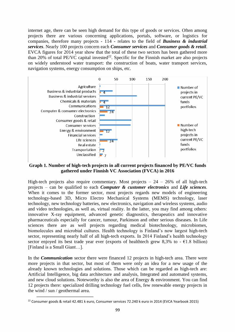
99

internet age, there can be seen high demand for this type of goods or services. Often among

projects there are various concerning applications, portals, software, or logistics for

companies, therefore many projects - 114 - relates to the field of Business & industrial

services. Nearly 100 projects concern each Consumer services and Consumer goods & retail.

EVCA figures for 2014 year show that the total of these two sectors has been gathered more

than 20% of total PE/VC capital invested22. Specific for the Finnish market are also projects

on widely understood water transport: the construction of boats, water transport services,

navigation systems, energy consumption on ships, etc.

Graph 1. Number of high-tech projects in all current projects financed by PE/VC funds

gathered under Finnish VC Association (FVCA) in 2016

High-tech projects also require commentary. Most projects – 24 – 26% of all high-tech

projects – can be qualified to each Computer & customer electronics and Life sciences.

When it comes to the former sector, most projects regards new models of engineering

technology-based 3D, Micro Electro Mechanical Systems (MEMS) technology, laser

technology, new technology batteries, new electronics, navigation and wireless systems, audio

and video technologies, as well as, virtual reality. In the latter, you may find among others:

innovative X-ray equipment, advanced genetic diagnostics, therapeutics and innovative

pharmaceuticals especially for cancer, tumour, Parkinson and other serious diseases. In Life

sciences there are as well projects regarding medical biotechnology, microbiomes,

biomolecules and microbial cultures. Health technology is Finland’s now largest high-tech

sector, representing nearly half of all high-tech exports. In 2014 Finland’s health technology

sector enjoyed its best trade year ever (exports of healthtech grew 8,3% to - €1.8 billion)

[Finland is a Small Giant…].

In the Communication sector there were financed 12 projects in high-tech area. There were

more projects in that sector, but most of them were only an idea for a new usage of the

already known technologies and solutions. Those which can be regarded as high-tech are:

Artificial Intelligence, big data architecture and analysis, Integrated and automated systems,

and new cloud solutions. Noteworthy is also the area of Energy & environment. You can find

12 projects there: specialized drilling technology fuel cells, few renewable energy projects in

the wind / sun / geothermal area.

22 Consumer goods & retail 42.481 k euro, Consumer services 72.240 k euro in 2014 (EVCA Yearbook 2015)

100

A systematic approach to promote innovation has been something that Finland has focused on

for many years. They implemented a national innovation strategy, various technology

programmes, and a network of regional science and technology parks. Finnish investment

funds and agencies plays an important role, in providing funds, expertise and information on

R&D and innovation projects [Herring P., 2013.].

Case of Polish PE/VC market

Venture capital is by definition an important source of financing innovative ideas that are

worth investing in. It is obvious that highly advanced technologies are the first to be taken

into account. The alarming fact is that investments in high-technologies in Poland are

extremely small and since 2013 do not reach even 1% of total PE/VC investments (table 4).

Table 4. The amount of PE/VC investments in high-tech in Poland, in 2010-2014 [in euro

k]

POLAND ( in € k) 2010 2011 2012 2013 2014 2015

Total investment 504

432

692

157

540

588

351

520

337

040

802

197

Subtotal High-Tech (amount) 318 21 502 21 277 3 199 2 736 7 755



In 2013 and 2014 the value of investments in highly developed technologies has not reached

even 1% of the total PE/VC investments. In comparison, in 2014 the average European share

of high-tech was 10.1% [EVCA 2015]. The reason might be: the risk aversion of Polish

PE/VC investors, which however stands in conflict with the definition of venture capital or

the insufficient number of ideas in this area that investors would be willing to support. On the

other hand, positive is the fact that the number of patents applications concerning strictly

high-tech industry, submitted by Poland at the European Patent Office is increasing and in

2013 it was 72 patent applications (the volume increased by 21% to the previous year)

[Eurostat 2014]. However, this amounts highly differ from the European average which is

approximately 200 high-tech patent applications in 2013 [Eurostat 2014].

Table 5 below represents an analysis of the portfolios of 48 funds operating in Poland,

grouped by national PE/VC association23. Around 300 projects considered concern only

Polish market. In 2016 all high-tech projects indicated in portfolios of Polish PE/VC finds

represents around 7% of total list of projects.

23 Poland – PSIK (Polskie Stowarzyszenie Inwestorów Kapitałowych)

101

Table 5. Portfolio analysis of Polish PE/VC funds’ gathered under Polish PE

Association (PSIK) in 2016

# of

PE/VC

funds

investing

in

particula

r sectors

# of

projects

in

current

PE/VC

funds

portfolio

s

# of

high-

tech

projects

in

PE/VC

funds

portfolio

s

Examples of projects from current PE/VC

fund portfolios connected with technology

area

Agriculture 0 1 0 n/a

Business &

industrial

products

18 31 1 binary Helix S.A. – high-technology

products

Business &

industrial

services

16 53 0 n/a

Chemicals &

materials 8 8 0 n/a

Communication

s 20 83 3

ORE S.A. - digital library and interactiv

education center

Dr Omnibus - tool for therapy and education

OptizenLabs - Modern digital media and

mobile applications

Computer &

consumer

electronics

11 18 5

WB Electronics S.A. - specialized

electronics and information military

3DKreator - rapid prototyping technology

Tech Sim Sp. z o.o. - modern flight

simulators

EgzoTech sp. z. o.o. - exoskeleton

FlyTech Solutions - innovative unmanned

systems

Construction 6 12 0 n/a

Consumer

goods & retail 14 25 0 n/a

Consumer

services 19 50 1 iTaxi - Modern taxi portal

Energy &

environment 10 14 0 n/a

Financial

services 9 20 0 n/a

Life sciences 20 34 9

HTL-Strefa – medical tools

ZdroweGeny.pl - Advanced genetic testing

BioTech – innovative dietary supplements

Smart Pharma - innovative medicines and

medical products

Laboratory Diagnostics - advanced

diagnostics

102

Biogenetica International Labolatories -

Innovative clinical trials

Numed Sp. z o.o. - Modern medical

equipment

novel-ID - The pharmaceutical

nanotechnology

Lifebrain - biotechnology

Real estate 3 3 0 n/a

Transportation 6 8 1

AERO AT Sp. z o.o. - aviation sector

Zakłady lotnicze MArgański & Mysłowski

SA – modern manufacture of aircrafts

Unclassified 5 6 2

Blue Dot Solutions Sp. z o.o - kconsulting in

the space sector

NanoVelos - nanotechnology

Total no. of

funds / projects 4824 36625 22

Source: Own based on data from particular funds webpages (funds lists available on: PSIK

http://www.psik.org.pl/fundusze.html) [access on 7.2016].

As the data in the table 5 stands, the largest number of investors are interested in the area life

sciences, communication and consumer services. While in the communication sector, there is

financed the largest number of projects - 83, in the health area there are currently funded 33

projects, which puts this sector at the 4th place. This is probably due to the fact that the

projects in the communication area relate largely to new software, new applications and are

relatively non-capital-consuming, while medical projects, e.g. setting up private clinics,

expansion of medical service offers, etc. require greater financial input. What is more in

software sector revenues are growing very fast – for leaders even by 600%-700% [22 polskie

firmy…].

Large amount of projects – 50 – regard Business & industrial services and Consumer

services. In 2014 consumer services gained over 30% of total PE/VC capital26. The rapid

development of networks and a significant increase in the availability of the Internet, is

boosting the creation of new solutions for consumers, based on the network, e.g. travel

agencies, insurance companies or comparison portalr, portals and platforms for learning etc.

24 The number is not the sum of the column, but the exact number of analysed PE/VC funds gathered in Polish PE Association. Some of the funds invest in variety of sectors. 25 Some of the projects were categorized to more than one sector, so the total number in the cell is bigger than the exact number of projects analysed. 26 103.608 k euro in 2014 (EVCA Yearbook 2015)


103

Graph 2. Number of high-tech projects in all current projects financed by PE/VC funds’

gathered under Polish VC Association (PSIK) in 2016

While analysing projects concerning strictly advanced/high technology, it's about 22 projects,

6% of all analysed projects, that can qualify to this area. As indicated in the table 5 and on the

graph 2 above, 9 of them concerns the health sector (life sciences). It is both a construction of

modern medical devices, biotechnology, advanced laboratory diagnostics (especially genetic)

and the area of pharmacy and pharmaceutical nanotechnology. Noteworthy is as well the

computers and electronics sector. You can find projects to create different kinds of

prototypes and simulators or specialist electronics for the military. What is more investments

such as consulting in the space sector, and nanotechnology (classified to a group of others, as

difficult to classify) are also interesting.

At the moment, high-tech entrepreneurs have greenhouse conditions. European and Polish

grants really allow funding of research leading to commercial products [Leszczyński M.,

2013]. However, many of development barriers of Polish high-tech sector, such as: improper

structure of expenditure on research and implementation of studies results, faulty structure of

scientists employment in industry sectors, high level of bureaucracy, level of the efficiency of

Polish scientific institutions, etc., cause that Polish companies are losing the global race,

despite a sizeable human potential [Chrzanowski K., 2013.]. However, interesting is the fact,

that in the 15th edition of the Forbes ranking - The Fastest Growing Technologically

Innovative Companies in Central Europe, 17 out of 50 companies were Polish (in main

category). Position of the leader in main category went to Hungarian company, but the second

prize - Polish company [22 polskie firmy…].

Case of Hungarian PE/VC market

In Hungary, the share in total PE/VC investments among years was much higher than e.g. for

Poland analysed before. However, alarming could be the fact, that the trend is declining since

2013.

104

Table 6. The amount of PE/VC investments in high-tech in Hungary, in 2010-2014 [in

euro k]

Hungary ( in € k) 2010 2011 2012 2013 2014 2015

Total investment 45 204 78 111 104 308 22 097 100 645 117 998

Subtotal High-Tech

(amount) 20 805 9 108 9 076 2 153 3 564 1 640



As negative can be taken fact that the number of high-tech patents applications, submitted by

Hungary to the European Patent Office is decreasing each year since 2011. In 2013 the value

was 26 applications [Eurostat 2014]. Buying licenses and patents for technological solutions

already proven are faster and cheaper, however, it do not influence directly on the Hungarian

market innovativeness, which is a room for improvement.

The table below represents an analysis of 24 PE/VC funds operating in Hungary, grouped by

Hungarian VC association27. More than 250 projects considered were dedicated mainly to

Hungarian market, but partially also to Czech and Slovakian market. In 2016 - 22 high-tech

projects listed in the table 7 represents almost 9% of all projects that attracted PE/VC funds.

Table 7. Portfolio analysis of Hungarian VC funds’ gathered under Hungarian VC

Association (HVCA) in 2016

Hungary

Number

of PE/VC

funds

investing

in

particular

sectors

Number

of

projects

in current

PE/VC

funds

portfolios

Number

of high-

tech

projects in

current

PE/VC

funds

portfolios

Examples of projects from current

PE/VC funds portfolios connected

with technology area

Agriculture 0 0 0 n/a

Business &

industrial

products

1 3 0 n/a

Business &

industrial

services

23 53 0 n/a

Chemicals &

materials 6 10 2

Pannon Tyre Recycling Ltd. - new tyre

recycling

Aquajet Zrt. - new rubber recycling

Communications 21 103 2

INTELLIO - new generation of

advanced video surveillance systems

LogMeIn - cloud based solutions

Computer &

consumer

electronics

12 14 5

AdasWorks - creating prototypes

Leopoly - new 3d solutions

NowTechnologies - new equipment

design

27 Hungary – HVCA Hungarian Venture Capital Association

105

Estimote Beacons - wireless sensors for

location

Polarisol Kft. - polarized light devices

Construction 3 3 0 n/a

Consumer goods

& retail 17 38 0 n/a

Consumer

services 11 24 0 n/a

Energy &

environment 6 11 0 n/a

Financial

services 5 6 0 n/a

Life sciences 17 45 12

AppCellTech Ltd. - Biotechnology

MDQuest Ltd. - R&D Biotechnology

StemLab - Preserver of umbilical cord

stem cells

NEBOTRADE - microbiology products

Kinestica - technology for neuromotoric

disorders

Medical Innovation Partners (MIP) -

developing pharmaceuticals

Baby Life Care - Advanced remote

embryo testing

Norma Instruments - innovative blood

analysis systems for in-vitro

PMP Technology - computer-controlled

dental labs

orthosera - cell therapies

Omixon - global molecular diagnostics

Aim Alliance Kft. - Biotechnology

Real estate 0 0 0 n/a

Transportation 3 5 0

Unclassified 1 1 1 BBS NANOTECH - nanotechnology

Total no. of

funds / projects 24 316 22

Source: Own based on data from particular funds webpages (funds lists available on: HVCA

http://www.hvca.hu/) [access on 7.2016].

Almost all funds grouped in the HVCA are interested in investing in the area of Business &

industrial services and Communications. By far the most - more than 100 projects – were

financed in the communication field, especially in mobile applications as well as forums and

social networking sites. As was mentioned earlier, these projects do not require significant

cash inflow, and taking into account the rapidly growing “mobile” market, the prognosis are

promising. Projects in the business services sector also attract capital. More than 53 projects

involving especially consulting, support for business systems and advanced networking

support management. Western European countries are increasingly being chosen by

multinational corporations, especially in the service sector. The area widely known as the life

sciences is also considered by venture capitalists to be interesting, as currently VC funds

finance about 45 projects in this area.

http://www.hvca.hu/

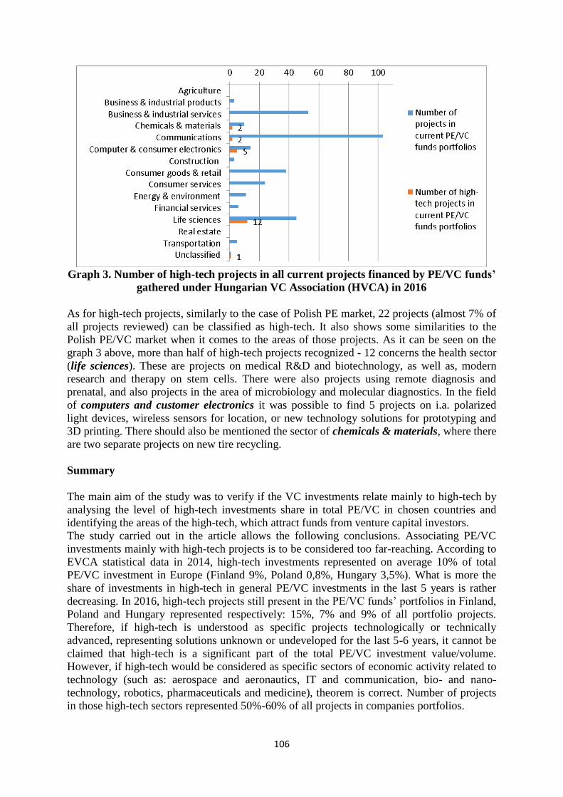
106

Graph 3. Number of high-tech projects in all current projects financed by PE/VC funds’

gathered under Hungarian VC Association (HVCA) in 2016

As for high-tech projects, similarly to the case of Polish PE market, 22 projects (almost 7% of

all projects reviewed) can be classified as high-tech. It also shows some similarities to the

Polish PE/VC market when it comes to the areas of those projects. As it can be seen on the

graph 3 above, more than half of high-tech projects recognized - 12 concerns the health sector

(life sciences). These are projects on medical R&D and biotechnology, as well as, modern

research and therapy on stem cells. There were also projects using remote diagnosis and

prenatal, and also projects in the area of microbiology and molecular diagnostics. In the field

of computers and customer electronics it was possible to find 5 projects on i.a. polarized

light devices, wireless sensors for location, or new technology solutions for prototyping and

3D printing. There should also be mentioned the sector of chemicals & materials, where there

are two separate projects on new tire recycling.

Summary

The main aim of the study was to verify if the VC investments relate mainly to high-tech by

analysing the level of high-tech investments share in total PE/VC in chosen countries and

identifying the areas of the high-tech, which attract funds from venture capital investors.

The study carried out in the article allows the following conclusions. Associating PE/VC

investments mainly with high-tech projects is to be considered too far-reaching. According to

EVCA statistical data in 2014, high-tech investments represented on average 10% of total

PE/VC investment in Europe (Finland 9%, Poland 0,8%, Hungary 3,5%). What is more the

share of investments in high-tech in general PE/VC investments in the last 5 years is rather

decreasing. In 2016, high-tech projects still present in the PE/VC funds’ portfolios in Finland,

Poland and Hungary represented respectively: 15%, 7% and 9% of all portfolio projects.

Therefore, if high-tech is understood as specific projects technologically or technically

advanced, representing solutions unknown or undeveloped for the last 5-6 years, it cannot be

claimed that high-tech is a significant part of the total PE/VC investment value/volume.

However, if high-tech would be considered as specific sectors of economic activity related to

technology (such as: aerospace and aeronautics, IT and communication, bio- and nano-

technology, robotics, pharmaceuticals and medicine), theorem is correct. Number of projects

in those high-tech sectors represented 50%-60% of all projects in companies portfolios.

107

When it comes to identifying the areas of high-tech projects, which attract funds from VC

investors, based on the portfolios of FVCA, PSIK and HVCA, there are two sectors which far

outweighs others: life sciences and computer & consumer electronics. They represents 59%

of all high-tech projects in PE/VC funds’ portfolios in Finland, Poland and Hungary.

Graph 4. Number of high-tech projects in PE/VC funds’ portfolios in Finland, Poland

and Hungary, in 2016.

Source. Own based on analysis results

There is, however, a lot of projects as well in the area of communications, energy &

environment, and nano- or bio-technology, which as per variety of applications, are usually

classified in “unclassified” sector.

Bibliography

1. Chrzanowski K., 2013. Polski przemysł high-tech - możliwości i bariery rozwoju, Sprawy

Nauki, [online] Available at

<http://www.sprawynauki.edu.pl/index.php?option=com_content&view=article&id=2488:pol

ski-przemys-high-tech-moliwoci-i-bariery-rozwoju&catid=304&Itemid=30>, [Accessed

August 2016]

2. Eurostat 2014. High-tech patent applications to the EPO by priority year [pat_ep_ntec],

[online] Available at

http://appsso.eurostat.ec.europa.eu/nui/show.do?dataset=pat_ep_ntec&lang=en [Accessed

August 2016]

3. Finland is a Small Giant of Medical Technology, 2014. [online], Available at

<http://www.finnishhealthtech.fi/industry-overview/42-industry/77-finland-is-a-small-giant-

of-medical-technology> [Accessed September 2016]

4. Grzegorczyk E., 2015. Private Equity/Venture Capital sector specifics in certain groups of

countries within Europe [in:] Mehmet H. Bilgin, H. Danis, E. Demir, U. Can (editors),

Business Challenges in the Changing Economic Landscape – Vol. 1. Proceedings for the 14th

Eurasia business and Economics Society Conference’ Eurasia Studies in Business and

Economics 2/1, Springer, pp.239-260.

http://appsso.eurostat.ec.europa.eu/nui/show.do?dataset=pat_ep_ntec&lang=en

108

5. Herring P., 2013. A great place to innovate in – and to invest in, HighTech Finland 2013,


<http://www.hightechfinland.com/direct.aspx?area=htf&prm1=1150&prm2=article>,

[Accessed August 2016]

6. Kopczewska K., Kopczewski T.,Wojcik P., 2009. Metody ilościowe: Aplikacje ekonomiczne

i finansowe. [Eng. Quantitative methods: Economic and financial implementations].

Warszawa: CeDeWu.

7. Leszczyński M., 2013. Polski hi-tech, [online], Available at

http://www.racjonalista.pl/kk.php/s,8798 [Accessed August 2016].

8. Słownik Języka Polskiego, PWN, [online] Available at < http://sjp.pwn.pl/slowniki/high-

tech.html> [Accessed August 2016]

9. Springer, Verzeichnis der Venture Economics Industry Codes , [online] Available at

http://download.springer.com/static/pdf/798/bbm%253A978-3-8349-4347-

7%252F1.pdf?originUrl=http%3A%2F%2Flink.springer.com%2Fbook%2Fbbm%3A978-3-

8349-4347-

7%2F1&token2=exp=1473538064~acl=%2Fstatic%2Fpdf%2F798%2Fbbm%25253A978-3-

8349-4347-

7%25252F1.pdf%3ForiginUrl%3Dhttp%253A%252F%252Flink.springer.com%252Fbook%

252Fbbm%253A978-3-8349-4347-

7%252F1*~hmac=1a7ae4d5644f4437d36772a7e375f62baf882b4af958649ddb495809c1e50d

b7 [Accessed 10.09.2016]

10. Zimny A., Inwestycje VC/PE w spółki high tech – trend długookresowy, Uniwersytet Łódzki,


<http://fin.czasopisma.pan.pl/images/data/fin/wydania/No_1_2012/Finanse%205-6-

A.Zimny.pdf> [Accessed August 2016]

11. 22 polskie firmy w rankingu Deloitte Fast 50, Forbes, [online], Available at

http://www.forbes.pl/22-polskie-firmy-w-rankingu-deloitte-fast-50,artykuly,184749,1,1.html,

[Accessed August 2016].

12. EVCA Yearbook 2015. European Private Equity Activity Data 2007-2014 [excel] Available

at <http://www.evca.eu/research/activity-data/annual-activity-statistics/> [Accessed 15

September 2016]

13. Invest Europe 2016, 2007-2015-dataset-europe-country-tables-public-version_final, [online]

Available at

https://www.google.pl/url?sa=t&rct=j&q=&esrc=s&source=web&cd=1&ved=0ahUKEwiz4c

6RxLfQAhXEOSwKHRe0DXsQFggpMAA&url=http%3A%2F%2Fwww.investeurope.eu%2

Fmedia%2F386098%2FYearbook-2015-Europe-Country-tables-Public-version-

FINAL.xlsx&usg=AFQjCNE--_tG4yt_poUbmJKd_YAFTA9cZw&sig2=7t8Lwy-

rumNVcH_Jw8evNA, [Accessed 29 September 2016]

http://www.hightechfinland.com/direct.aspx?area=htf&prm1=1150&prm2=article

http://www.racjonalista.pl/kk.php/s,8798

http://sjp.pwn.pl/slowniki/high-tech.html

http://sjp.pwn.pl/slowniki/high-tech.html

http://download.springer.com/static/pdf/798/bbm%253A978-3-8349-4347-7%252F1.pdf?originUrl=http%3A%2F%2Flink.springer.com%2Fbook%2Fbbm%3A978-3-8349-4347-7%2F1&token2=exp=1473538064~acl=%2Fstatic%2Fpdf%2F798%2Fbbm%25253A978-3-8349-4347-7%25252F1.pdf%3ForiginUrl%3Dhttp%253A%252F%252Flink.springer.com%252Fbook%252Fbbm%253A978-3-8349-4347-7%252F1*~hmac=1a7ae4d5644f4437d36772a7e375f62baf882b4af958649ddb495809c1e50db7









http://fin.czasopisma.pan.pl/images/data/fin/wydania/No_1_2012/Finanse%205-6-A.Zimny.pdf

http://fin.czasopisma.pan.pl/images/data/fin/wydania/No_1_2012/Finanse%205-6-A.Zimny.pdf

http://www.forbes.pl/22-polskie-firmy-w-rankingu-deloitte-fast-50,artykuly,184749,1,1.html

http://www.evca.eu/research/activity-data/annual-activity-statistics/

https://www.google.pl/url?sa=t&rct=j&q=&esrc=s&source=web&cd=1&ved=0ahUKEwiz4c6RxLfQAhXEOSwKHRe0DXsQFggpMAA&url=http%3A%2F%2Fwww.investeurope.eu%2Fmedia%2F386098%2FYearbook-2015-Europe-Country-tables-Public-version-FINAL.xlsx&usg=AFQjCNE--_tG4yt_poUbmJKd_YAFTA9cZw&sig2=7t8Lwy-rumNVcH_Jw8evNA





109

List of particular fund portfolios available at webpages published at HVCA Portal

<http://www.hvca.hu/>:

• http://3tscapital.com/

• http://www.ajh.hu/

• http://arxequity.com/

• http://www.bonitasktk.hu/

• http://www.buranvc.com/

• http://dbh-group.com/en/

• http://www.doclerinvestments.hu/

• https://www.ei.com.pl/hu/

• http://www.euroventures.hu/?lang=en

• http://www.finatech.hu/

• http://finext.hu/

• http://ieurope.com/

• http://www.krscapital.hu/

• http://www.mideuropa.com/

• http://pbgfmc.hu/

• http://portfolion.hu/?lang=en

• http://primuscapitalpartners.com/hu/

• http://www.riversideeurope.com/

• http://www.szta.hu/

• http://www.wallis.hu/

List of particular fund portfolios available at webpages published at PSIK Portal

<http://www.psik.org.pl/fundusze.html>:

• http://www.21concordia.com/

• http://3tscapital.com/

• http://www.abris-capital.com/

• http://www.adventinternational.pl/

• http://www.arxequity.com/

• http://www.avallon.pl/

• http://www.blackpearls.pl/

• http://www.bridgepoint.eu/

• http://www.seedfund.pl/

• http://www.c-p.pl/

• http://cee-equity.com/

• http://www.darbyoverseas.com/darby/index.jsp

• http://www.vestor.pl/kim-jestesmy

• http://www.ei.com.pl/pl/

• http://www.eqt.se/

• http://evf.com.pl/

• http://gpventures.pl/

• http://www.highlander-partners.com/

• http://www.ikinvest.com/

• http://www.imperasa.pl/

• http://www.innovacap.com/

• http://www.iqpartners.pl/

http://www.hvca.hu/

http://www.wallis.hu/


http://www.21concordia.com/

http://3tscapital.com/

http://www.abris-capital.com/

http://www.adventinternational.pl/

http://www.arxequity.com/

http://www.avallon.pl/

http://www.blackpearls.pl/

http://www.bridgepoint.eu/

http://www.seedfund.pl/

http://www.c-p.pl/

http://cee-equity.com/

http://www.darbyoverseas.com/darby/index.jsp

http://www.vestor.pl/kim-jestesmy

http://www.ei.com.pl/pl/

http://www.eqt.se/

http://evf.com.pl/

http://gpventures.pl/

http://www.highlander-partners.com/

http://www.ikinvest.com/

http://www.imperasa.pl/

http://www.innovacap.com/

http://www.iqpartners.pl/

110

• http://www.kfk.org.pl/

• http://www.krokuspe.pl/

• http://mci.pl/

• http://www.mezzmanagement.com/

• http://www.mideuropa.com/

• http://www.montagu.com/

• http://www.oresaventures.com/

• http://www.pentonpartners.com/

• http://www.pinebridge.com/

• http://www.rp.com.pl/?id=1

• http://www.resourcepartners.eu/en

• http://www.riversidecompany.com/

• http://www.royalton-partners.com/

• http://www.satus.pl/

• http://www.secus.pl/

• http://www.skyline.com.pl/

• http://http//speedupinnovation.com/

• http://www.syntaxis-capital.com/

• http://value4capital.com/

• http://www.warburgpincus.com/

• http://www.warsawequity.com/

• http://www.waterland.nu/

• http://www.wsicapital.pl/

List of particular fund portfolios available at webpages published at FVCA Portal

<http://www.fvca.fi/>:

• http://www.3i.com/

• http://www.aboaventure.fi/

• http://adelisequity.com/en/

• http://www.altor.com/

• http://armadamezzanine.com/

• http://www.auratum.com/aura-capital/aura-capital

• http://butterfly.vc/

• http://www.canelco.fi/fi/etusivu/

• http://www.capman.com/

• http://www.conor.vc/

• http://www.eqt.fi/

• http://www.essedel.com/

• http://www.helmetcapital.fi/

• http://www.industrikapital.com/

• http://www.innovestorgroup.com/

• http://interapartners.fi/

• http://www.invenicapital.com/

• http://inventure.fi/

• http://ipr.vc/

• http://www.juuripartners.fi/#yritys

• http://www.koronainvest.fi/en/

http://www.kfk.org.pl/

http://www.krokuspe.pl/

http://mci.pl/

http://www.mezzmanagement.com/

http://www.mideuropa.com/

http://www.montagu.com/

http://www.oresaventures.com/

http://www.pentonpartners.com/

http://www.pinebridge.com/

http://www.rp.com.pl/?id=1

http://www.resourcepartners.eu/en

http://www.riversidecompany.com/

http://www.royalton-partners.com/

http://www.satus.pl/

http://www.secus.pl/

http://www.skyline.com.pl/

http://http/speedupinnovation.com/

http://www.syntaxis-capital.com/

http://value4capital.com/

http://www.warburgpincus.com/

http://www.warsawequity.com/

http://www.waterland.nu/

http://www.wsicapital.pl/

http://www.fvca.fi/

111

• http://www.lifelineventures.com/

• http://www.mbrahastot.fi/fi/

• http://www.midinvest.fi/en/

• http://www.nexitventures.com/

• http://www.nordiamanagement.fi/

• http://www.nordiccapital.com/

• http://www.nordicmezzanine.com/

• http://www.noweco.fi/

• http://openoceancapital.com/

• http://www.pontos.fi/

• http://www.profitagroup.fi/

• http://reaktorventures.com/

• http://www.sentica.fi/

• http://www.sievicapital.fi/web/

• http://www.sponsor.fi/

• http://straightforward.vc/#home

• http://www.teollisuussijoitus.fi/

• http://www.triton-partners.com/

• http://www.vaakapartners.fi/

• http://www.ventechvc.com/

• http://vntm.com/

• http://www.wallstreet.fi/

112

THE PRINCIPAL-AGENT PROBLEM IN HEALTH CARE SYSTEMS: IS IT

EFFECTED BY PERFORMANCE-BASED SUPPLEMENTARY PAYMENT

SYSTEM?

Emre Atilgan

Trakya University, Turkey


Abstract

Health service systems exhibit certain features which distinguish them from regular markets.

One of the most important features of health care markets is the principle-agent problem that

arises from information asymmetries between health care supply and demand. Accordingly,

the demand for health care services is argued as a physician-led phenomenon. In Turkey,

after implementation of the Health Transformation Program (HTP) in 2003, the demand and

also the expenditure for the healthcare services considerably increased, but however the

increase in health care supply, e.g. the physician supply, increased in slight scale. The sub

reform of performance-based supplementary payment system (PBSPS), which was

implemented at the beginning of 2004, is seen as the most important effect of the rise in

healthcare services demand, in which the performance payments of physicians are be bound

up to the output they generate. The aim of this paper is to empirically investigate the

principle-agent problem for the Turkish health system, considering the PBSPS reform. The

Bound test approach, autoregressive distributed lag approach (ARDL) and Kalman Filter

Modelling are employed for the 1975-2013 period to examine the co-integration relationship,

between the health care demand and supply in Turkey.

Key Words: Principal-agent problem, Health System Reforms, Bound Test; ARDL Model;

Kalman Filter Method.

I. Introduction

Health service systems exhibit certain features which distinguish them from regular markets.

One of the most important features of health care markets is the principle-agent problem that

arises from information asymmetries between health care supply and demand. An agency

relationship as a contract under which one or more persons (the principal(s)) engage another

person (the agent) to perform some service on their behalf which involves delegating some

decision-making authority to the agent (Jensen & Meckling, 1976). In health care services,

citizens lack information about the range and efficacy of treatments. Even expert collective

purchasers of health services, such as insurance organizations, find it difficult to judge

whether services are being provided according to their preferences (Smith, Stepan,

Valdmanis, & Verheyen, 1997). As the patients do not have perfect knowledge of their

medical condition, their need for care, or the expected outcome of health care services, they

are willing to have physicians act as their agents in providing information and services

(Petersen, Woodard, Urech, Daw, & Sookanan, 2006). In the relationship between the

physician and the patient, the patient (the principle) delegates his/her health problem to the

physician (the agent). On the other hand, the agent has his own utility function, which he

maximizes. This utility function may coincide partly with the utility function of the principle,

but may also differ (Ludwig, Van Merode, & Groot, 2010). Thus the demand for health care

services is argued as a physician-led phenomenon.


113

In Turkey, after implementation of the Health Transformation Program (HTP) in 2003, the

demand and also the expenditure for the healthcare services considerably increased, but

however the increase in health care supply, e.g. the physician supply, increased in slight

scale. The sub reform of performance-based supplementary payment system (PBSPS), which

was implemented at the beginning of 2004, is seen as the most important effect of the rise in

healthcare services demand, in which the performance payments of physicians are be bound

up to the output they generate.

The aim of this paper is to empirically investigate the principle-agent problem for the Turkish

health system, considering the PBSPS reform. The Bound test approach, autoregressive

distributed lag approach (ARDL) and Kalman Filter Modelling are employed for the 1975-

2013 period to examine the co-integration relationship, between the health care demand and

supply in Turkey.

The rest of the paper is organized as follows. Section II introduces data and methodology.

Section III presents empirical results and the last section concludes.

II. Data and Methodology

In the study, two variables are used to test the validity of the principle-agent problem and the

physician-led health demand issue in Turkey, for the years 1970-2013. The variable CONS is

the number of per capita consultations in a year, which is used to represent healthcare

demand. The variable DR, representing the healthcare supply, is the number of Physicians

(per 1,000 people). The data for the variables are obtained from OECD statistics and The

Word Bank Statistics portal, for the variables CONS and DR respectively. All variables are

measured in natural logarithms for the analysis. Two other dummy variables are described to

capture the effect of two important health policy implementation in Turkey. The first dummy

variable is used to capture the effect of Green Card and named as DUM_GRN which has the

values of “0” for the years 1970-1991, and “1” for the rest. The second dummy variable

DUM_PERF is used to capture the effect of PBSPS and has the has the values of “0” for the

years 1970-2003, and “1” for the rest.

In the empirical analysis, three econometric models are used to investigate the relationship

between healthcare demand and supply, after stationarity checks for the variables. The

stationary properties of the CONS and DR are diagnosed both by conventional unit root tests

including ADF, PP and Ng-Perron tests.

In the first stage of analysis, the Bound test approach28 proposed by Pesaran et al. (2001) is

used to check the validity of co-integration relationship between variables. After co-

integration analysis, in the second stage, ARDL approach is used to investigate the long and

short- term static relationship between per capita physicians and per capita consultations.

ARDL model specification for the estimates is as in the equation 1:

0 1 2 3 3

1 0

m n

t i t i i t i t

i i

CONS CONS DR DUMGRN DUMPERF

(1)

In the third stage of the analysis, in order to estimate the dynamic relationship between

variables, the Kalman filter approach is used to explore the time-varying interaction between

28 The bounds testing approach has several advantages over conventional co-integration methods. First the Bound testing approach is applicable irrespective of whether the regressors are purely I(0) or I(1) (Pesaran, Shin, & Smith, 2001). Secondly, this approach presents efficient and superior results for small sample (Narayan & Narayan, 2004).

114

CONS and DR. The dynamic model used in this study is based on a classical reference of

Harvey (1989) with the Kalman filter approach with a form of state space representation.

III. RESULTS

Unit Root Tests

The stationarity properties of the variables are diagnosed both by using the conventional unit

root tests including ADF (Dickey & Fuller, 1979), PP (Phillips & Perron, 1988), and Ng-

Peron (Ng & Perron, 2001) tests. The results of stationary tests are presented in Table 1

below. According to Table 1, all conventional unit root tests shows that CONS and DR

variables are stationary after differencing so that CONS and DR series are I(1).

Table 1: Conventional Unit Root Test Results

ADF Test Results PP Test Results

Variable t-stat Prob t-stat Prob

CONS -1.471 0.825 -1.476 0.823

DR -0.747 0.963 -2.892 0.175

ΔCONS -5.389 0.000 -5.389 0.000

ΔDR -8.151 0.000 -7.858 0.000

Ng-Perron Test Results

Variable MZa MZt MSB MPT

CONS 1.411 1.141 0.809 51.452

DR 0.941 0.796 0.847 51.126

ΔCONS -15.113 -2.739 0.181 1.660

ΔDR -11.012 -2.277 0.207 2.491

Ng-Peron critical values for CONS and DR series; MZa, MZt, MSB, MPT

respectively;

%5 significance level : -17.30, -2.91, 0.17 and 5.48.

Ng-Peron critical values for ΔCONS and ΔDR series; MZa, MZt, MSB, MPT

respectively;

%5 significance level: -8.10, -1.98, 0.23 and 3.17

Bound Test Co-Integration Approach

In this study, the Bound testing co-integration approach is chosen due to its advantages over

conventional cointegration methods, which are stated above. Table 3 shows the bound test

results.

Table 3. Bound Test Results

K* F-statistics

Critical Value at %5 Significance

Level

Bottom Bound Upper Bound

1 10.65 4.94 5.73

*k is the number of the independent variables in equation 1.

Critical values are taken from Table C1.iii at Pesaran et al.

(2001, p. 300)

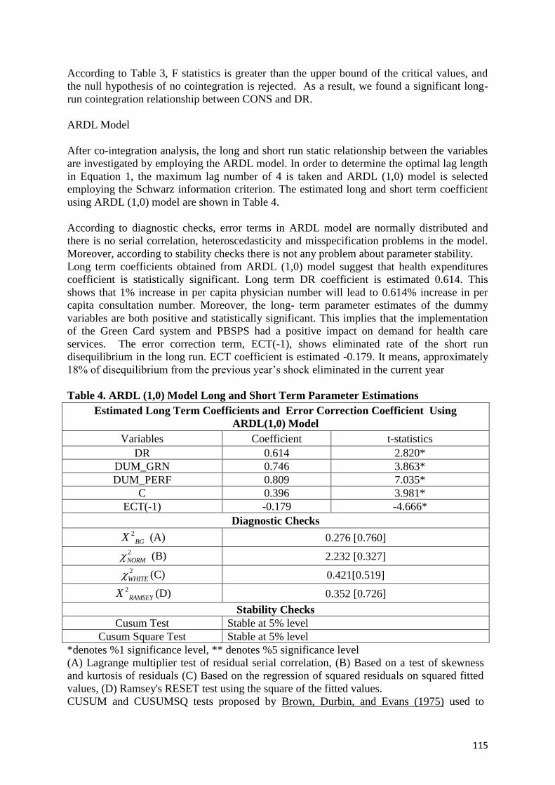
115

According to Table 3, F statistics is greater than the upper bound of the critical values, and

the null hypothesis of no cointegration is rejected. As a result, we found a significant long-

run cointegration relationship between CONS and DR.

ARDL Model

After co-integration analysis, the long and short run static relationship between the variables

are investigated by employing the ARDL model. In order to determine the optimal lag length

in Equation 1, the maximum lag number of 4 is taken and ARDL (1,0) model is selected

employing the Schwarz information criterion. The estimated long and short term coefficient

using ARDL (1,0) model are shown in Table 4.

According to diagnostic checks, error terms in ARDL model are normally distributed and

there is no serial correlation, heteroscedasticity and misspecification problems in the model.

Moreover, according to stability checks there is not any problem about parameter stability.

Long term coefficients obtained from ARDL (1,0) model suggest that health expenditures

coefficient is statistically significant. Long term DR coefficient is estimated 0.614. This

shows that 1% increase in per capita physician number will lead to 0.614% increase in per

capita consultation number. Moreover, the long- term parameter estimates of the dummy

variables are both positive and statistically significant. This implies that the implementation

of the Green Card system and PBSPS had a positive impact on demand for health care

services. The error correction term, ECT(-1), shows eliminated rate of the short run

disequilibrium in the long run. ECT coefficient is estimated -0.179. It means, approximately

18% of disequilibrium from the previous year’s shock eliminated in the current year

Table 4. ARDL (1,0) Model Long and Short Term Parameter Estimations

Estimated Long Term Coefficients and Error Correction Coefficient Using

ARDL(1,0) Model

Variables Coefficient t-statistics

DR 0.614 2.820*

DUM_GRN 0.746 3.863*

DUM_PERF 0.809 7.035*

C 0.396 3.981*

ECT(-1) -0.179 -4.666*

Diagnostic Checks 2

BGX (A) 0.276 [0.760]

2

NORM (B) 2.232 [0.327]

2

WHITE (C) 0.421[0.519]

2

RAMSEYX (D) 0.352 [0.726]

Stability Checks

Cusum Test Stable at 5% level

Cusum Square Test Stable at 5% level

*denotes %1 significance level, ** denotes %5 significance level

(A) Lagrange multiplier test of residual serial correlation, (B) Based on a test of skewness

and kurtosis of residuals (C) Based on the regression of squared residuals on squared fitted

values, (D) Ramsey's RESET test using the square of the fitted values.

CUSUM and CUSUMSQ tests proposed by Brown, Durbin, and Evans (1975) used to

116

Dynamic Approach – Kalman Filter

The Kalman filter model used in this study is presented in equations 2 and 3 below.

0 1, 2, 3,t t t t t tLY a a LH a DUMGRND a DUMPERF (2)

, , 1 ,i t i t i ta a v (3)

The time varying parameter estimates for health expenditures by employing Kalman Filter

approach are shown in Figure 1. The dynamic parameter estimates for the variable DR are

found to be also statistically significant. The results show that per capita physician number

has a positive and increasing effect on per capita consultation especially after the first years

of Health Transformation Program (HTP) and PBSPS. Thus the estimated dynamic

parameters of DR are compatible with static coefficient.

According to the TVP estimates of Kalman filter approach, the effect of DR on CONS

decreased between 1979 and 1998 and increased in the period of 1999-2003. In the first four

years of HTP and, which covers the first 2 years of PBSPS, the dynamic parameters decline.

But after 2007, as can be seen from the upward trend of the dynamic parameters, the effect of

DR on CONS increases considerably.

Figure 1: Time Varying Parameter (TVP) Estimates for Kalman Filter Approach

IV CONCLUSION

In this study, a stable long-run cointegration between the healthcare service supply and

demand is found for Turkey for the years 1975-2013. The results of the ARDL model suggest

that an increase in the number of physicians per capita leads an increase for health care

demand, namely number of consultations per capita. Additionally, two other policy

implementations, the Green Card System and Performance Based Supplementary Payment

System, is found to have positive and statistically significant effect on health care demand.

To this respect, this study offers some primitive evidence for the proposal which states that

the demand for health care services is as a physician-led phenomenon due to the principal-

agent problem. On the other hand, these results should also be compared with the results of

another model that is extended by using microeconomic tools. Thus, the need for further

research in this area remains profound.

examine the presence of parameter stability

117

REFERENCES

1. Brown, R., Durbin, J., & Evans, J. (1975). Techniques for testing the constancy of regression

relationships over time. Journal of the Royal Statistical Society, 37, 149-192.

doi:10.2307/2984889

2. Dickey, D. A., & Fuller, W. A. (1979). Distribution of the estimators for autoregressive time

series with a unit root. Journal of th American Statistical Association, 74, 427-431.

doi:10.2307/2286348

3. Harvey, A. C. (1989). Forecasting. Structural time series models and the Kalman Filter.

4. Jensen, M. C., & Meckling, W. H. (1976). Theory of the firm: Managerial behavior, agency

costs and ownership structure. Journal of Financial Economics, 3, 305-360.

doi:10.1016/0304-405X(76)90026-X

5. Principal agent relationships and the efficiency of hospitals., 11 291-304 (2010).

6. Narayan, P., & Narayan, S. (2004). Is there a long-run relationship between exports and

imports? Evidence from two Pacific Island countries. Economic Papers, 23, 152-164.

7. Ng, S., & Perron, P. (2001). LAG Length Selection and the Construction of Unit Root Tests

with Good Size and Power. Econometrica, 69, 1519-1554. doi:10.1111/1468-0262.00256

8. Pesaran, M. H., Shin, Y., & Smith, R. J. (2001). Bounds testing approaches to the analysis of

level relationships. Journal of Applied Econometrics, 16, 289-326. doi:10.1002/jae.616

9. Petersen, L. A., Woodard, L. D., Urech, T., Daw, C., & Sookanan, S. (2006). Does pay-for-

performance improve the quality of health care? Annals of internal medicine, 145(4), 265-

272.

10. Phillips, P. C., & Perron, P. (1988). Testing for a unit root in time series regression.

Biometrika, 75, 335-346. doi:10.1093/biomet/75.2.335

11. Smith, P. C., Stepan, A., Valdmanis, V., & Verheyen, P. (1997). Principal-agent problems in

health care systems: an international perspective. Health Policy, 41(1), 37-60.

118

THE DETERMINANTS OF BORROWING BEHAVIORS OF TURKISH

MUNICIPALITIES

Hakan Yaş



Emre Atilgan



Abstract

Municipalities in Turkey being categorized as metropolitan, nonmetropolitan, and district and

town municipalities, have substantially increased their borrowing amounts in the past ten

years. Having regard to the fact that the flypaper theory exists in municipalities in Turkey,

they are spending pretty much under the influence of non-matching financial transfers. The

more the borrowing amounts of local governments increase, the more the public expenditures

grow. Moreover, Turkish municipalities may respond more impulsively in borrowing as there

is not a golden rule confining them regarding the quantity of borrowing. Thus, the substantial

growth in local borrowing may have a boosting effect on total public expenditures. The

object of this paper is to analyze whether any other determinants or factors are affecting the

borrowing behaviors of municipalities in Turkey. The determinants of the borrowing

behavior relating to the analysis are selected as financial transfers, own revenues, and

expenditures of municipalities, to achieve the object. The Bound test and autoregressive

distributed lag (ARDL) approaches are employed for the 2007 – 2014 period quarterly to

examine the co-integration relationship between the borrowing and its determinants.

Keywords: Intergovernmental transfers, local borrowing, flypaper effect, ARDL Model

1. Introduction

Local authorities are self – governing units so as to designate adequate financial resources of

their own, and these resources should be commensurate with the responsibilities provided for

by the constitution and the law, according to European Charter of Local Self – Government

(Council of Europe, 1985). In Turkey, the autonomy of local governments and adequate

financial resources to be commensurately provided within the scope of their responsibilities

are ensured by the Constitution and the Law No.5393. Although Turkey adopted the Chart,

also was chary of a number of articles of the Chart, such as sufficiently diversification of

resources allocated for local governments, and provision of grants not to remove their basic

freedom. Article 74 of the Constitution of the Republic of Turkey explicitly states that

“Taxes, fees, duties, and other such financial obligations shall be imposed, amended, or

revoked by law”. According to the article, local governments are not capable of levying tax or

such financial obligations on the local public as the Assembly is the unique supreme body for

imposing, amending or revoking financial issues. Another constitutional obligation for local

finance ensured in Article 127 is that the local governments shall be allocated financial

resources in proportion to their functions. These legal arrangements denote a structure for

local governments on the one hand to be a fiscally autonomous authority, on the other hand

having limited power to designate their own revenues.



119

Local governments, however, have an enormous expenditure increasing particularly in last

decade. Because of lack of fiscal autonomy, local governments could defray these

expenditures by either receiving financial transfers (grants) from central government or

borrowing domestically or from abroad. The studies resulted that the flypaper effect exists in

Turkish municipalities, the most authorized local government tier, which means that

municipalities in Turkey are given to financial transfers rather than their own revenues in

meeting their responsibilities. This complex situation denotes that it could not be claimed

that local governments in Turkey have a financial autonomy in practice. So it is obvious that

self – government of local authorities in Turkey remains a fiscal problem.

This study aims to analyze the determinants or factors affecting the borrowing behaviors of

municipalities (metropolitan, nonmetropolitan, and district and town municipalities) in

Turkey. A direct relation is normally expected between expenditures and borrowing. Because

of the existence of flypaper effect, own revenues and financial transfers are also involved in

the estimation model in addition to the expenditures. In the direction of the literature,

expenditures and financial transfers are expected to increase the borrowing whereas the

increase in own revenues is expected to reduce the borrowing amount.

Financial Data Trend of Municipalities in Turkey

Municipalities in Turkey have a great number of responsibilities to be met. But however, they

are not able to design their own revenues as mentioned above. Municipal Revenues Law No.

2464 itemizes the most of the own revenues of municipalities. The Law No. 5779 designates

the rate and distribution criteria of the financial transfers on the basis of municipality types

separately. The main criterion in allocating the transfers is the population of the municipality,

by affecting the 80% of the share. The remaining 20% is bound up the rank of the

municipality in the provincial development index which is specified by Ministry of

Development. These transfers consist of revenue sharing amounts and grants from central to

local level. The Municipal Law No. 5393, however, establishes the rules of borrowing of

municipalities. There is not a golden rule on local government borrowing in Turkey. The

Golden Rule is defined as “local governments should not borrow to finance current

expenditures but investment expenditures” (Swianiewicz, 2004, pp. 5-9; Council of Europe,

1985). Moreover, Municipal Law states “A municipality can borrow and issue bond in order

to finance its expenditures required for its assignments and services…” Nothing but foreign

borrowing is subject to such a golden rule; foreign borrowing is allowed only for financing

projects included in the investment program. There is, however, some limitations demarked

in The Law No. 5393, such as total amount of debt of a municipality including debt of its

corporations and its affiliates shall not exceed their total budget receipts augmented by annual

revaluation rate.

Figures 1, 2 and 3 indicates the change and the trend of financial data including borrowing

and expenditures on all three types of municipalities in Turkey totally. As shown in Figure 1,

the borrowing amounts of municipalities approximately multiplied eight times beginning

from 2007Q1 to 2014Q4. The jump in the own revenues and the financial transfers in the last

two quarters is due to change in the number of metropolitan municipalities.

120

Figure 1: Change in Financial Transfers, Own Revenues and Borrowing Amounts

(2007Q1-2014Q4)

The borrowing amounts of municipalities is a stock variable, whereas the amounts of

financial transfers and own revenues are changing by the beginning of the budget year.

Besides the legal amendments relating financial transfers and own revenues, the borrowing

amount changes are in parallel with the increase in the expenditures. Figure 2 shows that the

increase in borrowing amounts is greater than the increase in debt stock of municipalities.

Figure 2: Change in Borrowing and Debt Stock Amounts (2007Q1-2014Q4)

Figure 3 indicates both the change and the trend of the expenditures made by all types of

municipalities in Turkey. %90 of total borrowing amount is composed of the loans received

by municipalities from İlbank Inc., the primary creditor of the municipalities, which is the

only local government bank in Turkey for over eighty years.

121

Figure 3: Change and Trend in Expenditures (2007Q1-2014Q4)

2. Literature Review

Flypaper effect can be explained by the expression that intergovernmental financial transfers

affect the increase in local government spending more than the own revenues do. Although

there are studies that indicate the flypaper effect on municipalities in Turkey exist (Aytaç,

2015; Sağbaş & Saruç, 2004; Yaş & Akduğan, 2015), there is not such a study analyzing the

effect of financial transfers or expenditures on borrowing associated with own revenues and

expenditures. There are some foreign studies suggesting that fiscal dependency ratio –the

share of intergovernmental transfers and grants in total local government revenues– causes to

higher borrowing costs and burden (De Mello, 2001). In a previous study(Yaş & Atılgan,

2016), it is suggested that a rise in the financial transfers given to municipalities causes a rise

in the long-run borrowing of the municipalities in Turkey as these governments neither are

able to determine their own revenues nor can increase the amount of the financial transfers

because of the legal limitations.

3. Data and Method

In this study, to test the fly paper effect theory, an ARDL model is specified and estimated

using quarterly data for the municipalities for the years 2007-2014. In the analysis, the total

borrowing amount of the municipalities is the dependent variable and named as BOR. Three

independent variables used in the ARDL model. First one is FT, which accounts the total

financial transfers from central government to municipalities. The second variable OWN is

the own revenues of the municipalities. The third variable EXP is the total expenditures of

the municipalities. All the variables used in the analysis is expressed in natural logarithms.

As the variables FT, OWN and EXP has seasonal effects, these variables are seasonally

adjusted by using the Tramo/Seats methodology.

In the first stage of the empirical analysis, the stationary properties of the variables BOR, FT,

OWN and EXP are diagnosed by unit root tests including ADF, PP and Ng-Perron tests. Then

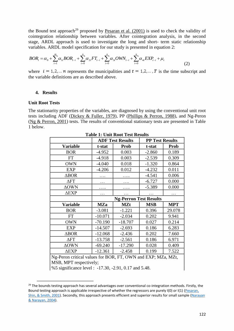
122

the Bound test approach29 proposed by Pesaran et al. (2001) is used to check the validity of

cointegration relationship between variables. After cointegration analysis, in the second

stage, ARDL approach is used to investigate the long and short- term static relationship

variables. ARDL model specification for our study is presented in equation 2:

0 1 2 3 4

1 0 0 0

m n n n

t i t i i t i i t i i t i t

i i i i

BOR BOR FT OWN EXP

(2)

where represents the municipalities and is the time subscript and

the variable definitions are as described above.

4. Results

Unit Root Tests

The stationarity properties of the variables, are diagnosed by using the conventional unit root

tests including ADF (Dickey & Fuller, 1979), PP (Phillips & Perron, 1988), and Ng-Peron

(Ng & Perron, 2001) tests. The results of conventional stationary tests are presented in Table

1 below.

Table 1: Unit Root Test Results

ADF Test Results PP Test Results

Variable t-stat Prob t-stat Prob

BOR -4.952 0.003 -2.860 0.189

FT -4.918 0.003 -2.539 0.309

OWN -4.040 0.018 -1.320 0.864

EXP -4.206 0.012 -4.232 0.011

ΔBOR …. ….. -4.541 0.006

ΔFT … …. -6.727 0.000

ΔOWN ….. ….. -5.389 0.000

ΔEXP … … … …

Ng-Perron Test Results

Variable MZa MZt MSB MPT

BOR -3.081 -1.221 0.396 29.078

FT -10.071 -2.034 0.202 9.941

OWN -70.190 -18.707 0.027 0.214

EXP -14.507 -2.693 0.186 6.283

ΔBOR -12.068 -2.436 0.202 7.660

ΔFT -13.758 -2.561 0.186 6.971

ΔOWN -69.240 -17.290 0.028 0.409

ΔEXP -12.361 -2.458 0.199 7.522

Ng-Peron critical values for BOR, FT, OWN and EXP; MZa, MZt,

MSB, MPT respectively;

%5 significance level : -17.30, -2.91, 0.17 and 5.48.

29 The bounds testing approach has several advantages over conventional co-integration methods. Firstly, the Bound testing approach is applicable irrespective of whether the regressors are purely I(0) or I(1) (Pesaran, Shin, & Smith, 2001). Secondly, this approach presents efficient and superior results for small sample (Narayan & Narayan, 2004).

123

Ng-Peron critical values for ΔCONS and ΔDR series; MZa, MZt,

MSB, MPT respectively;

%5 significance level: -8.10, -1.98, 0.23 and 3.17

According to Table 1, unit root tests suggest different results for the variables. The variable

BOR is found to be I(0) according to ADF test but I(1) according to PP test. This same result

is also obtained for the variables FT and OWN. EXP variable is found to be I(0) according to

all unit root tests.

Bound Test Cointegration Approach

Conventional unit root tests suggest different results for the variables. Therefore, we choose

employing the Bound testing co-integration approach proposed by Pesaran et al. (2001), as

this approach could be used irrespective of whether the regressors are purely I(0) or I(1).

Table 2 shows the bound test results.

Table 2. Bound Test Results

K F

statistics

Critical Value at %5

Significance Level

Bottom Bound Upper

Bound

3 15.13 3.23 4.35

k is the number of independent variables in equation 1. Critical values are taken from Table

C1.iii at Pesaran et al. (2001, p. 300)

According to Table 2, F statistics is greater than the upper bound of the critical values, and

the null hypothesis of no cointegration is rejected. As a result, we found a significant long

run cointegration relationship between the borrowing and its determinants.

ARDL Model

After co-integration analysis, the long and short run static relationship between the variables

are investigated by employing the ARDL model. In order to determine the optimal lag length

in Equation 1, by taking the maximum lag number as 4, ARDL (3,1,4,3) model is selected

employing the Schwarz information criterion. The estimated long-run coefficients of ARDL

(3,1,4,3) model are shown in Table 3.

124

Table 3. ARDL (3,1,4,3) Model Long and Short Term Parameter Estimations

According to diagnostic checks, error terms in ARDL model are normally distributed and

there is no serial correlation, heteroscedasticity and misspecification problems in the model.

Moreover, according to stability checks, there is not any problem about parameter stability.

According to ARDL (3.1,4,3) model, the estimated long-run coefficient of FT is not

statistically significant. Long-term coefficient of OWN is -1.926 (p<0.05), which means that

1% increase in the own revenues of municipalities will lead %1.93 decrease in the total

borrowing amount. Additionally, the estimated long-run coefficient of EXP shows that 1%

increase in the expenditure of municipalities causes 4.49% rise in the total borrowings

(p<0.05). The coefficient of the error correction term (ECT (-1)), which shows eliminated

rate of the short run disequilibrium in the long-run, is estimated -0.421. Therefore, we found

that the speed of adjustment of a disequilibrium from the previous year’s is eliminated within

the next year.

5. Conclusion

In the previous study (Yaş & Atılgan, 2016) in which a panel data framework including all

types of municipalities in Turkey is implemented, presented that there is a long-run

relationship from financial transfers to both short and long-term borrowing amounts of

municipalities. Contrariwise the previous, time series analysis is used and the total amount of

borrowing of metropolitan and nonmetropolitan provincial municipalities are analyzed in this

paper, without separating borrowing amounts to short and long components. Moreover,

Estimated Long Term Coefficients and Error Correction Coefficient

Using ARDL(4,4,3,4) Model

Variables Coefficient Prob

FT -1.339 0.091

OWN -1.926 0.003

EXP 4.489 0.000

C -6.453 0.000

ECT(-1) -0.421 0.000

Diagnostic Checks 2

BGX (A) 0.618 [0.556]

2

NORM (B) 0.799 [0.670]

2

WHITE (C) 0.289 [0.746]

2

RAMSEYX (D) 0.829 [0.595]

Stability Checks

Cusum Test Stable at 5% level

Cusum Square Test Stable at 5% level

(A) Lagrange multiplier test of residual serial correlation, (B) Based on a

test of skewness and kurtosis of residuals (C) Based on the regression of

squared residuals on squared fitted values, (D) Ramsey's RESET test using

the square of the fitted values.

CUSUM and CUSUMSQ tests proposed by Brown, Durbin, and Evans

(1975) is used to examine the presence of parameter stability

125

expenditures and own-revenues of municipalities are also included in this model. Therefore,

the effect of financial transfers over borrowing could not be sighted for this model.

The results of the analysis suggest that an increase in own revenues of the municipalities

lowers their borrowing requirement. In contrast, an increase in municipal expenditures raises

the borrowing amount of the municipalities. These results are in parallel with the expectation

related to Turkish municipalities. As the maximum amount of financial transfers and the

ability to obtain the own revenues is limited within in the laws No. 5779 and Constitution

respectively, the municipalities concentrate on borrowing as a last resort in order to defray

the growing expenditures.

In order to suggest a policy proposal, if the local self – government issue in Turkey is going

to be intimately resolved, then the capability of designating their own revenues have to be

allowed for local governments in less than no time. Slightly limited borrowing can lead a

moral risk for local authorities. Public debt, otherwise, may grow enormously owing to

increase in local borrowing amounts.

References

1. Aytaç, D. (2015). Türkiye'de Yönetimler Arası Transferler Sinek Kağıdı Etkisi Yaratıyor

Mu? Ampirik Bir İnceleme. Yönetim ve Ekonomi Araştırmaları Dergisi, 13(2), 166-180.

2. Brown, R., Durbin, J., & Evans, J. (1975). Techniques for testing the constancy of regression

relationships over time. Journal of the Royal Statistical Society, 37, 149-192.

doi:10.2307/2984889

3. Council of Europe. (1985). European charter of local self-government. Strasbourg: European

Treaty Series - No. 122.

4. De Mello, L. R. (2001). Fiscal decentralization and borrowing costs: the case of local

governments. Public Finance Review, 29(2), 108-138.

5. Dickey, D. A., & Fuller, W. A. (1979). Distribution of the estimators for autoregressive time

series with a unit root. Journal of th American Statistical Association, 74, 427-431.

doi:10.2307/2286348

6. Narayan, P., & Narayan, S. (2004). Is there a long-run relationship between exports and

imports? Evidence from two Pacific Island countries. Economic Papers, 23, 152-164.

7. Ng, S., & Perron, P. (2001). LAG Length Selection and the Construction of Unit Root Tests

with Good Size and Power. Econometrica, 69, 1519-1554. doi:10.1111/1468-0262.00256

8. Pesaran, M. H., Shin, Y., & Smith, R. J. (2001). Bounds testing approaches to the analysis of

level relationships. Journal of Applied Econometrics, 16, 289-326. doi:10.1002/jae.616


Biometrika, 75, 335-346. doi:10.1093/biomet/75.2.335

10. Sağbaş, İ., & Saruç, T. (2004). Intergovernmental Transfers and the Flypaper in Turkey.

Turkish Studies, 5(2), 79-92.

126

11. Swianiewicz, P. (2004). The theory of local borrowing and the West-European experience.

Local government borrowing: risks and rewards: a report on Central and Eastern Europe.

New York: Open Society Institute.

12. Yaş, H., & Akduğan, U. (2015). Türkiye'de Belediyelere Yapılan Mali Transferlerin Flypaper

Effect Çerçevesinde İncelenmesi. Maliye Dergisi(168), 49-68.

13. Yaş, H., & Atılgan, E. (2016). Do Intergovernmental Financial Transfers Have An Effect

Upon Municipal Borrowing? Subsequent Effect of Flypaper Theory in Municipalities in

Turkey. Paper presented at the The IIER International Conference on Social Science and

Economics (ICSSE), Athens.

127

THE IMPORTANCE OF EFFECTIVE SOCIOECONOMIC CONDITIONS,

GOVERNMENT POLICIES AND PROCEDURES FACTORS FOR

ENTREPRENEURIAL ACTIVITY:

(USING FUZZY ANALYTIC HIERARCHY PROCESS IN EIGHT DEVELOPING

COUNTRIES)

Iman Aghaei



Amin Sokhanvar



Mustafa Tümer



Abstract

The aim of present research is to determine how environmental factors in terms of

entrepreneurial activity can be effective in developing countries. While developing, countries

are becoming a renowned force in international entrepreneurship; there is a distinct need to

know the most important indicators that influence entrepreneurial activities. Lately, there are

many literatures about entrepreneurship, but most of them do not consider the features of

entrepreneurial activity, especially in developing countries. This research evaluates some

effective socioeconomic conditions and government policies and procedures indicators which

influence the level of entrepreneurial activity. For this purpose, 287 individuals of population

selected as sample from the case countries, thereafter, questionnaires were distributed and

collected data among them. This study proposes an integrated approach of multiple criteria

decision making (MCDM) method and fuzzy analytic hierarchy process (FAHP) using the

pairwise comparisons between criteria to derive the true weights from a fuzzy comparison

matrix. Based on the empirical results of this study, commercial and services infrastructure,

opportunities to business start-up and unemployment rate have the greatest relative impact on

the level entrepreneurial activity summary for the case study, respectively.

Keywords: Environmental factors, Entrepreneurial activity, Fuzzy-AHP model, Developing

countries

1. Introduction

Traditionally, there has been no bold contrast for notions of management and

entrepreneurship. However, the entrepreneurship has addressed to small business start-up and

management for most of the twentieth century (Morris et al., 1996). Entrepreneurship was

introduced by specialists as a way to reinvigorate economies and assist the economic growth

in many developing countries (Spencer and Gómez, 2004). As Stevenson, et al., (1985)

argue, the entrepreneurship denoted by means of “the process of creating value by bringing

together unique combinations of resources to exploit an opportunity”. Nevertheless,

entrepreneurship and small business are not synonymous perceptions literally, but they are




128

linked together. In entrepreneurial activity perspective, entrepreneurs engage opportunities

instead resources (Thurik and Wennekers, 2004). Even though there has been

“entrepreneurship” by means of a significant term in business framework there about two

centuries, but the meaning has converted during the time (Morris et al., 1996). Wennekers

and Thurik (1999) describe entrepreneurs are persons who recognize new economic

opportunities. In face of uncertainty, they employ their ability and desire to take hold of

opportunities through their particular activity into the market.

Newly, following of economy growth is in the spotlight. In this circumstance, growth is

defined by a substantial rise in sales, profits, assets, employees, and/or locations. The

entrepreneurial firm is one that proactively strive to develop, and is not restricted by the

resources under its control at present (Morris et al., 1996). A broad letter has occurred

considering firm entry and exit which is commonly applied to measure entrepreneurial

activity as well as pragmatic work, since effectual work on the entrance in Canadian

manufacturing (De Backer and Sleuwaegen, 2003).

Later research focused on characters of individuals as the indicators impact on

entrepreneurial activity. The main concerning was costs of own business formation. Recent

researchers investigate that organizational constitutions affect national levels (Specht, 2003).

It is possible to apply entrepreneurial activity as a conditional factor to entrepreneurship

research by particular conditions such as social, economic and policies (Minaev, 2016). In

spite of its applied value, there is no sufficient realization that which factors impress on high

rates of entrepreneurship in a country, then how governments are able to boost

entrepreneurial activity in domestic economies (Spencer and Gómez, 2004).

Certainly, it cannot be overlooked the effective relationship between the growth and

prosperity of the societies (Bjørnskov,and Foss, 2010). According to Birch and McCracken’s

(1987) findings, the entrepreneurial sector was demonstrated “as a relatively small subset of

the small business sector”. In recent times, the preference of many people is starting a firm

rather than salaried outside organizations. For this reason, entrepreneurial activities were

promoted by public administration to simplify creative business establishment procedures

and academics through their research support to design the public policies (Alvarez et al.,

2011). The members’ manner of society to make decision for becoming an entrepreneur can

be affected considerably by attitudes, values and principals belong to that society (Shapero

and Sokol, 1982). According to sociological or institutional approach, environment plays the

critical role in starting a business. This is not only about public policies or legal aspects, but

also pertains to the socio-cultural perspective (Alvarez et al., 2011). As clearly exposed by

Lucas (1973), whenever the national income level is enlarged consequently the average size

of domestic companies will be increased. According to the above investigation, for the

advancement of entrepreneurship, different organizations have made known special policies

and strategies. Simultaneously, academic researchers are concerned that determine effective

factors on entrepreneurial activity (Alvarez and Urbano, 2011).

This paper concentrates to rank of the crucial environmental factors on the entrepreneurial

activity. In this regards, all societies are not the same in lots of respects. Commonly, in this

type of cases, the socioeconomic development classification is applied for performing the

researches (Minaev, 2016). Gnyawali and Fogel (1994) recommended the framework for the

entrepreneurial environment which includes government policies and procedures,

socioeconomic factors, entrepreneurial and business skills, and financial and non-financial

assistance along with their effective sub-factors. Minaev (2016:4) describe that the “lack of

129

entrepreneurial sector trends” is the principal drive to research in developing countries,

because many difficulties are available in procedure of creating own business for people. As

well as environmental conditions the economies situation can fluctuate every year. There is

no precise approach to tracing the trend of entrepreneurial activity index in many developing

countries. In doing so, it is imaginable to reflect more unchanging indicators which stimulus

entrepreneurial activity in addition to unexpected statuses (Minaev, 2016).

The present research focuses on two groups of environmental conditions, which can affect

the index of entrepreneurial activity as follows: Socioeconomic and government policies and

procedures. If majority of society’s sight about entrepreneurship to be with distrust,

entrepreneurship may not succeed. Motivation of entrepreneurs to creation a new firm is a

foundation of prevalent communal support and desirable outlook of people to

entrepreneurship. Indeed, social conditions as principle as ease to reach of information,

finances, technical aid and tangible services (Gnyawali and Fogel, 1994). In 1988, Mokry’s

findings show that the local communities have the vital impress in entrepreneurial

environment development. Likewise, Societies and cultures have a tendency to grow public

systems to encourage entrepreneurship (Vesper, 1983). The countries with potent

entrepreneurial environment may also empower to attract foreign aids such as technology

(Spencer and Gómez, 2004:1100). Economic circumstances also have to impact the rate of

self-employment in a society. The higher unemployment rate in a country, the larger

stimulant is the cause of exploring the self-employment opportunities (Evans and Leighton,

1990; Wildeman et al., 1998). However, self-employment phenomenon is probably

publicized in developing countries.

Findings show the entrepreneurial business activities are more likely to entail “advanced

manufacturing technique” and “economics of scale” that is like obstacles for business start-

ups. Wholly, some criteria such as unemployment rate and per capita GDP can influence on

entrepreneurial activities (Spencer and Gómez, 2004). The economic meters such as

“entrepreneurial activity” are usually assessment tools of entrepreneurship (Minaev, 2016).

Moreover, market mechanisms productivity can affect by government policies through

eliminating conditions that cause executive inflexibilities and market failures. They can also

form an “enterprise culture” that empowers businesses to take rational risks and search for

profits. While, there are numerous rules and procedures to start an innovative business or

entrepreneurs may become hopeless to pursue them and if they have to take more time and

cost to meet the requirements (Dana, 1987, 1988; Young and Welsch, 1993).

2. Literature Review:

Krzysztof Wach (2015) made a study about considering the impact of social and cultural

indicators toward entrepreneurship, according to the data related to the Global

Entrepreneurship Monitor’s (GEM) report on 2013. In the European Union, entrepreneurial

activity was inspected in 23 countries. The outcomes of the study show: in entrepreneurial

culture, innovation-oriented and efficiency-oriented economies of European Union are not

different. The willingness of people to use entrepreneurial opportunities to launch a business

which leads to an increase in entrepreneurial activity, as hypothesis two was confirmed.

Based on the other supported hypothesis, there is the low level of necessity-driven

entrepreneurship in cultures with developed level of the entrepreneurial environment.

A research is also conducted by Hessels, van Gelderen, Thurik (2008) to answer the question

whether the reasons are to start their own business and the level of social security of the

country to explain the prevalence of entrepreneurial aspirations. The cross-country analysis is

130

performed on global Entrepreneurship Monitor data (GEM) for 29 countries in 2005. The list

of countries is Argentina, Australia, Austria, Belgium, Brazil, Canada, Chile, Denmark,

Finland, France, Germany, Greece, Hungary, Iceland, Ireland, Italy, Japan, Mexico,

Netherlands, New Zealand, Norway, Slovenia, South Africa, Spain, Sweden, Thailand,

United Kingdom, United States, and Venezuela. The outcomes explained the adverse

influence of social security level on people’s entrepreneurial intentions. Furthermore, the

positive correlation was discovered from findings between the rise in motivation to gather

prosperity and entrepreneurial aspirations with regard to employment and export growth.

In 2000, the multivariate logistic regression analysis was carried out by Thomas and Mueller

for the case of 8 countries (USA, Canada, Ireland, Belgium, China, Singapore, Slovenia and

Croatia) to explore the relationship between main individuals and culture characteristics on

entrepreneurial activity. In addition to culture feature, the human creativity, a sense of self-

control, the propensity for risk and activity of the individual had been implemented. In this

case the entrepreneurs were appeared more dynamic. As a result, a sense of self-control is the

most important indicators for entrepreneurial activity in individualistic societies in the high

level of satisfaction the large effect on the motivation of public to become, if entrepreneurs

are tendency to risk.

The research about the foreign direct investment incentives entrepreneurial activity was

conducted by Kim and Li (2014). The authors also consider because of socio-political

conditions, the relationship differs across countries. They were analyzed dependent count

variable and time-varying covariates for 104 countries from 2000 to 2009 by using a panel

negative-binomial model. They declare entrepreneurial activity as the level of firm

establishment for the duration of a specified period of time. This construct in terms of the

annual number of lately registered limited-liability businesses was measured in each country.

As a conclusion, the positive benefits on firm formation are strongest in districts with weak

institutional infrastructures and low entire educational procuration.

McMullan, Bagby and Palich (2008) have published an article entitled “economic freedom

and motivation to engage in entrepreneurial activity”. In their study, by applying institutional

theory, they analyzed opportunity-motivated entrepreneurial activity (OME) and necessity-

motivated entrepreneurial activity (NME) on 10 indicators of economic liberty and gross

domestic product (GDP) per capita for 37 countries. The results depict that OME and NME

are correlated negatively to GDP and with labor freedom positively. The researchers explain

entrepreneurial activity affect from governmental limitations for economic liberty in a

different way depending on the specific freedom constrained by government and the

entrepreneur’s motivation for employing in entrepreneurial action.

Grossman and Shapiro (1984) have analyzed the effect of foreign investment on the business

creation of domestic entrepreneurs in an open economy, even though the most occupational

choice models have been studied in a closed economy situation. In Grossman’s research

illustrates that falling the numbers of domestic entrepreneurs as the result of lower prices on

the market are affected by import competition and foreign direct investment. Subsequently,

entrepreneurial income becomes less than the wage income.

Measuring the weights of environmental factors is a major issue as well as a driving force of

the discussion on entrepreneurial activity context. Developing evaluation criteria and

methods that reliably measure environmental framework is a prerequisite for focusing the

more effective factors on entrepreneurial activity. The multiplicity of criteria and measuring

131

tools being developed in this fast-growing field shows the importance of the conceptual and

methodological work in this area. The development and selection of factors require

parameters related to the reliability, appropriateness, practicality and limitations of

measurement. The used criteria to evaluate the environmental factors in the literatures mainly

divide to two groups: Socioeconomic conditions, government policies and procedures which

are summarized in Table (1). The first dimension includes per capita income, unemployment

rate, education and training, public attitude toward entrepreneurship, diversity of economic,

opportunities to business start-up. Another dimension comprises entry barriers, political

stability, procedures for starting a business, commercial and services infrastructure, market

openness, Intellectual property rights. We purpose to estimate the weights of environmental

conditions and their sub-factors which impact the level of entrepreneurial activity in

developing countries through fuzzy approach of analytic hierarchy process. Finally, we

present the results which will be depicted the weights of these factors using data from eight

developing countries.

Table 1: The effective environmental conditions and factors on entrepreneurial activity

3. Data sample and methodology:

Since this research, by collecting the dimensions and factors has created the possibility of

deciding over the effective socioeconomic conditions and government policies factors on

entrepreneurial activities, though, this research, objective–wise is applicable. But

methodology-wise, this research due to the description of the criteria and alternative

decisions creates the possibility of subject’s analysis and decision making, so it is considered

as descriptive – analytic research.

In the first step of this research we identified the environmental dimensions and factors

influencing the entrepreneurial activities brand by using the library methodology and valid

databases and relevant scientific scripts. The identified criterion was distributed within the

Delphi questionnaire among the experts who were asked to comment on the factors’ refusal

or confirmation. They were also asked to consider adding up some other factors in the

questionnaire besides the ones identified. After completing the questionnaire, the confirmed

factors were selected by experts as the final ones which were compared with separate

Environmental conditions Factors Literatures

Socioeconomic conditions Per capita income (Hessels and van Stel, 2011);

(Bjørnskov,and Foss, 2010);

(Spencer and Gómez, 2004);

(Alvarez and Urbano, 2011)

Unemployment rate (Acs and Armington);

(Audretsch and Keilbach,

2004); (Morris et al., 1996);

(Spencer and Gómez, 2004);

(Alvarez et al., 2011)

Education and Training (Alvarez et al., 2011)

Public attitude toward entrepreneurship (Gnyawali and Fogel, 1994)

Diversity of economic (Gnyawali and Fogel, 1994)

Opportunities to business start up (Alvarez et al., 2011)

Government policies and

procedures

Entry barriers (Gnyawali and Fogel, 1994)

Political stability (Alvarez and Urbano, 2011)

Procedures for starting a business (Alvarez and Urbano, 2011)

Commercial and services infrastructure (Alvarez et al., 2011)

Market openness (Alvarez et al., 2011)

Intellectual property rights (Alvarez et al., 2011)

132

standard AHP questionnaires in pairwise comparisons. This methodology gives an analytic

procedure that can join and solidify the assessments of the choices and criteria by either an

individual or group included in the task of decision making. It should be noted that the two

elements that are compared at a particular time largely reduces the conceptual complexity of

the analysis, we provide empirical evidence of the impact of socioeconomic conditions and

government policy key factors and procedures on entrepreneurial activity, in eight of

developing countries. We collected 287 respondents divided into eight countries, the Algeria,

Egypt, Iran, Libya, Nigeria, North Cyprus, Tajikistan and Turkey, respectively, 31, 32, 42,

35, 37, 35, 35, and 40. The age range of the respondents varied between 20 and 55. With

regarding to job experience, respondents divided into five groups. According to this

classification, there were 15 percent is lower than 5 years, 22 percent is 5 to 10 years, 31

percent is between 10 and 15 years, 22 percent is 15 to 20 years, and finally 10 percent is

more than 20 years. Some professionals on the subject were asked to contribute to the

research by completing the questionnaire to reduce bias.

Analytic hierarchy process (AHP) (Saaty, 1988) has been broadly used as an advantageous

multiple criteria decision making (MCDM) tool or a weight estimation technique in many

areas such as selection, evaluation, planning and development, decision making, forecasting,

and so on. The traditional AHP requires crisp judgments. A number of methods have been

developed to handle fuzzy comparison matrices. Among the above approaches, the extent

analysis method has been employed in quite a number of applications due to its

computational simplicity. However, such a method is found unable to derive the true weights

from a fuzzy or crisp comparison matrix. The weights determined by the extent analysis

method do not represent the relative importance of decision criteria or alternatives at all.

Therefore, it should not be used as a method for estimating priorities from a fuzzy pairwise

comparison matrix. The theory of Saaty’s (1980) priority for fuzzy extension has applied by

many researchers. Then Laarhoven and Pedrycg (1983) suggested the fuzzy comparing

judgment with triangular fuzzy numbers. Chang (1996) proposed an extent analysis method

on fuzzy-AHP to obtain a crisp priority vector from a triangular fuzzy comparison matrix. It

is found that the extent analysis method cannot estimate the true weights from a fuzzy

comparison matrix and has led to quite a number of misapplications in the literature (Wang et

al., 2008).

In this article, by applying Chang’s (1996) new approach to conduct fuzzy-AHP, the priority

vectors for environmental dimensions and sub-factors determined by the extent analysis

method. Initially, triangular fuzzy numbers are implemented for pairwise comparison scale.

Thereafter, through the extent analysis method, the synthetic extent value Si of pairwise

comparison, weight vectors in terms of each factor under a certain dimension can be

computed.

4. Results

After the conversion of qualitative variables to triangular fuzzy numbers M On R: [1/9, 9]

that its membership is (l, m, u), where l ≤ m ≤ u, l and u exist for lower and upper bond of the

support of M respectively, and m for the modal value (Chang, 1996). A triangular fuzzy

comparison matrix demonstrated by (Wang et al., 2008):

133

If, (l, m, u) = a is a triangular fuzzy number, the inverse form will be as follows:

The preliminary matrix of pairwise comparisons for environmental dimensions and their sub-

factors after data integration will be shown in table (2-1), (2-2) and (2-3) as follows: Table 2-1: Fuzzy comparison matrix of two environmental dimensions after data integration

dimensions D1 D2

D1 (1.00, 1.00, 1.00) (0.11, 2.42, 9.00)

D2 (0.11, 0.41, 9.00) (1.00, 1.00, 1.00)

Whose data provide:

• D1: Socioeconomic conditions

• D2: Government policies and procedures

Table 2-2: Fuzzy comparison matrix of six socioeconomic factors after data integration

factors SE1 SE2 SE3 SE4 SE5 SE6

SE1 (1.00, 1.00, 1.00) (0.11, 0.23, 6.00) (0.11, 0.26, 5.00) (0.20, 3.22, 9.00) (0.11, 0.57, 8.00) (0.25, 3.89, 9.00)

SE2 (0.17, 4.44, 9.00) (1.00, 1.00, 1.00) (0.20, 7.14, 9.00) (4.00, 8.62, 9.00) (0.50, 6.95, 9.00) (2.00, 8.25, 9.00)

SE3 (0.20, 3.86, 9.00) (0.11, 0.14, 5.00) (1.00, 1.00, 1.00) (4.00, 7.72, 8.00) (0.11, 2.37, 9.00) (0.50, 5.43, 9.00)

SE4 (0.11, 0.31, 5.00) (0.11, 0.12, 0.25) (0.13, 0.13, 0.25) (1.00, 1.00, 1.00) (0.13, 0.25, 5.00) (0.14, 0.25, 6.00)

SE5 (0.13, 1.76, 9.00) (0.11, 0.14, 2.00) (0.11, 0.42, 9.00) (0.20, 4.08, 8.00) (1.00, 1.00, 1.00) (3.00, 7.20, 9.00)

SE6 (0.11, 0.26, 4.00) (0.11, 0.12, 0.50) (0.11, 0.18, 2.00) (0.17, 3.94, 7.00) (0.11, 0.14, 0.33) (1.00, 1.00, 1.00)

Whose data provide:

• SE1: Per capita income

• SE2: Opportunities to business start up

• SE3: Unemployment rate

• SE4: Public attitude toward entrepreneurship

• SE5: Education and Training

• SE6: Diversity of economic

Table 2-3: Fuzzy comparison matrix of six government policy factors after data integration

factors GP1 GP 2 GP 3 GP 4 GP 5 GP 6

GP 1 (1.00, 1.00, 1.00) (5.00, 8.43, 9.00) (0.50, 6.32, 9.00) (6.00, 8.77, 9.00) (5.00, 8.89, 9.00) (2.00, 9.00, 9.00)

GP 2 (0.11, 0.12, 0.20) (1.00, 1.00, 1.00) (3.00, 7.20, 9.00) (0.11, 0.57, 8.00) (0.25, 3.89, 9.00) (0.11, 0.26, 5.00)

GP 3 (0.11, 0.16, 2.00) (0.11, 0.14, 0.33) (1.00, 1.00, 1.00) (2.00, 8.25, 9.00) (4.00, 7.72, 9.00) (0.50, 5.43, 9.00)

GP 4 (0.11, 0.11, 0.17) (0.13, 1.76, 9.00) (0.11, 0.12, 0.50) (1.00, 1.00, 1.00) (0.20, 3.22, 9.00) (0.20, 3.42, 9.00)

GP 5 (0.11, 0.11, 0.20) (0.11, 0.26, 4.00) (0.11, 0.13, 0.25) (0.11, 0.31, 5.00) (1.00, 1.00, 1.00) (0.14, 0.25, 6.00)

GP 6 (0.11, 0.11, 0.50) (0.20, 3.86, 9.00) (0.11, 0.18, 2.00) (0.11, 0.29, 5.00) (0.17, 3.94, 7.00) (1.00, 1.00, 1.00)

Whose data provide:

• GP1: Commercial and services infrastructure

• GP2: Political stability

134

• GP3: Market openness

• GP4: Procedures for starting a business

• GP5: Entry barriers

• GP6: Intellectual property rights

Chang (1996) defined in the next step, the value of synthetic extent as Si vector should be

calculated. To obtain the first vector, we accumulate together the components of fuzzy

numbers in each row. In the second vector, the total sum of the existing triangular numbers in

the above matrix turned to their reverse form. This vector is the same in all Si calculations.

Such vector is the multiplication product of two vectors which is calculated. Considering the

above description, the vectors Si will be calculated in table (3-1), (3-2) and (3-3) as follows:

Table 3-1: degree of possibility of for environmental dimensions

S1 (0.0556,0.7074,4.5000)

S2 (0.0556,0.2926,4.5000)

Table 3-2: degree of possibility of for socioeconomic factors

S1 (0.0091,0.1037,1.6277)

S2 (0.0403,0.4118,1.9704)

S3 (0.0303,0.2322,1.7562)

S4 (0.0083,0.0232,0.7496)

S5 (0.0223,0.1652,1.6277)

S6 (0.0082,0.0638,0.6354)

Table 3-3: degree of possibility of for government policies and procedures

S1 (0.1095,0.4274,1.2486)

S2 (0.0257,0.1314,0.8740)

S3 (0.0433,0.2287,0.8234)

S4 (0.0098,0.0971,0.7781)

S5 (0.0089,0.0208,0.4465)

S6 (0.0095,0.0946,0.6650)

Subsequently, based on Wang et al., (2008)’ findings usage is for comparing the degree of

possibility of Si vectors in algorithm of fuzzy hierarchical analysis compute by the following

equation:

Where

Thus, the comparison of vectors S1 to S6 of the above formula will be shown in table (4-1),

(4-2) and (4-3) as follows:

Table 4-1: Comparison Si vectors for environmental dimensions

S1 ≥ S2 S2≥S1

1.0000 0.9146

135

Table 4-2: Comparison Si vectors for socioeconomic factors

S1 ≥ S2, S3, S4, S5, S6 S2 ≥ S1, S3, S4, S5, S6 S3 ≥ S1, S2, S4, S5, S6 S4 ≥ S1, S2, S3, S5, S6 S5 ≥ S1, S2, S3, S4, S6 S6 ≥ S1, S2, S3, S4, S5

0.8482 1.0000 1.0000 0.9022 1.0000 0.9402

0.9309 1.0000 0.9055 0.6470 0.8659 0.6320

1.0000 1.0000 1.0000 0.7754 0.9598 0.7828

0.9658 1.0000 1.0000 0.8369 1.0000 1.0000

Table 4-3: Comparison Si vectors for government policies and procedures factors S1 ≥ S2, S3, S4, S5, S6 S2 ≥ S1, S3, S4, S5, S6 S3 ≥ S1, S2, S4, S5, S6 S4 ≥ S1, S2, S3, S5, S6 S5 ≥ S1, S2, S3, S4, S6 S6 ≥ S1, S2, S3, S4, S5

1.0000 0.7209 0.7823 0.6694 0.4533 0.6254

1.0000 0.8951 1.0000 0.9565 0.7919 0.9457

1.0000 1.0000 1.0000 0.8481 0.6598 0.8226

1.0000 1.0000 1.0000 1.0000 0.8512 0.9962

The degree possibility for convex fuzzy number to be larger than k convex fuzzy numbers Mi

(I = 1, 2, …, k) can be determined in table (5-1), (5-2) and (5-3) as follows:

V (M ≥ M1, M1, …, Mk)

= V [(M ≥ M1) and (M ≥ M2) and … and (M ≥ Mk)

= min V (M ≥ Mi), i = 1, 2, …, k.

d’(Ai) = min V (Si ≥ Si), k = 1, 2, …, n; k ≠ i

Table 5-1: d’(Ai) values for environmental dimensions

Table 5-2: d’(Ai) values for socioeconomic factors

Table 5-3: d’(Ai) values for government policies and procedures factors

According to Chang method, then the weight vector is given by:

W’ = (d’ (A1), d’ (A2), …, d’ (An)) T

Where Ai (I = 1, 2, …, n) are n elements.

Via normalization, we can get the normalized weight vectors:

W = (d (A1), d (A2), …, d (An)) T

d’ (A1) = Min (S1 ≥ S2) 1.0000

d’ (A2) = Min (S2 ≥ S1) 0.9146

d’ (A1) = Min (S1 ≥ S2, S3, S4, S5, S6) 0.8482

d’ (A2) = Min (S2 ≥ S1, S3, S4, S5, S6) 1.0000

d’ (A3) = Min (S3 ≥ S1, S2, S4, S5, S6) 0.9055

d’ (A4) = Min (S4 ≥ S1, S2, S3, S5, S6) 0.6470

d’ (A5) = Min (S5 ≥ S1, S2, S3, S4, S6) 0.8659

d’ (A6) = Min (S6 ≥ S1, S2, S3, S4, S5) 0.6320

d’ (A1) = Min (S1 ≥ S2, S3, S4, S5, S6) 1.0000

d’ (A2) = Min (S2 ≥ S1, S3, S4, S5, S6) 0.7209

d’ (A3) = Min (S3 ≥ S1, S2, S4, S5, S6) 0.7823

d’ (A4) = Min (S4 ≥ S1, S2, S3, S5, S6) 0.6694

d’ (A5) = Min (S5 ≥ S1, S2, S3, S4, S6) 0.4533

d’ (A6) = Min (S6 ≥ S1, S2, S3, S4, S5) 0.6254

136

Where W is a nonfuzzy number. The final weight vectors will be depicted in table (6-1), (6-

2) and (6-3): Table 6-1: final matrix for environmental dimensions

W’ (1.0000,0.9146) T

W (0.5223,0.4777)

Table 6-2: final matrix for socioeconomic factors W’ (0.8482,1.0000,0.9055,0.6470,0.8659,0.6320) T

W (0.1732,0.2041,0.1849,0.1321,0.1768,0.1290)

Table 6-1: final matrix for government policies and procedures factors

W’ (1.0000,0.7209,0.7823,0.6694,0.4533,0.6254) T

W (0.2352,0.1696,0.1840,0.1575,0.1066,0.1471)

The end result can be obtained from the multiplication of weight of each factor into related

dimension. Thus, based on the fuzzy-AHP Technique, the priorities of the effective

socioeconomic conditions and government policies and procedures on entrepreneurial

activity are illustrated in table (7) as follows:

Table 7: Prioritization weight of effective environmental factors summary for case study

Factor relative important Total relative important

GP1 Commercial and services infrastructure 0.1124

SE2 Opportunities to business start up 0.1066

SE3 Unemployment rate 0.0965

SE5 Education and Training 0.0923

SE1 Per capita income 0.0904

GP3 Market openness 0.0879

GP2 Political stability 0.0810

GP4 Procedures for starting a business 0.0752

GP6 Intellectual property rights 0.0703

SE4 Public attitude toward entrepreneurship 0.0690

SE6 Diversity of economic 0.0674

GP5 Entry barriers 0.0509

5. Conclusion:

At the company level, standing literature has recognized the influence of environmental

factors on business efficiency (Covin and Slevin, 1991; Venkatraman and Prescott, 1990;

Zahra, 1993). The discussions advanced recommend that alike contacts may exist between

environmental factors and individual entrepreneur’s performance, and matching between

specific entrepreneurs’ requirements and environmental forces would lead to bigger

likelihood of firm creation and achievement.

It was addressed among the environmental conditions two main dimensions as

socioeconomic and government policy and procedures. Even though, further factors were

available for each dimension, but according to scholars’ opinions, six remarkable indicators

were chosen from previous literatures. We attempted to find out the weight of each condition,

and their sub-indicators. The weight from evaluation for each dimension to each factor

affects the ranking of the design from formulating the data given.

Based on the drawn results, the commercial and services infrastructure highest one, where the

total relative important is 0.1124 compared with eleven others. In continue, opportunities to

business start-up, unemployment rate, education and training, and per capita income

137

respectively have the next major effect for the level of entrepreneurial activity. The rest of

factors, market openness, political stability, procedures for starting a business, Intellectual

property rights, public attitude toward entrepreneurship, diversity of economic, entry barriers

are the next order.

However, due to the complexity and uncertainty involved in real world decision problems,

entrepreneurship decision and policy makers may sometimes feel more confident to provide

fuzzy judgments than crisp comparisons. A decision maker can be used this integrates fuzzy-

AHP outputs to enhance the level of entrepreneurial activities in a nation.

Certainly, this study was carried out for 8 developing countries because we did not access

enough information about countries. Meanwhile, applying the fuzzy-AHP method is a new

approach for entrepreneurship development. For future research, we suggest that the

interested researcher can study about others developing countries to reach the more accurate

information for making a better decision toward entrepreneurship environment. Considering

the most important elements cause to faster growing with regard to motivate and support

entrepreneurs in countries.

Acknowledgment The authors would like to acknowledge the Center for Entrepreneurship and Innovation of

Eastern Mediterranean University (http://gimer.emu.edu.tr) for supporting this study.

References

1. Acs, Z., & Armington, C. (2004). Employment growth and entrepreneurial activity in

cities. Regional Studies, 38(8), 911-927.

2. Acs, Z. J., & Armington, C. (2003). Endogenous growth and entrepreneurial activity in

cities. Washington, DC: Center for Economic Studies, Bureau of the Census.

3. Acs, Z. J., Desai, S., & Hessels, J. (2008). Entrepreneurship, economic development and

institutions. Small business economics, 31(3), 219-234

4. Acs, Z. (2006). How is entrepreneurship good for economic growth? Innovations, 1(1),

97-107.

5. Alvarez, C., Urbano, D., Coduras, A., & Ruiz-Navarro, J. (2011). Environmental

conditions and entrepreneurial activity: a regional comparison in Spain. Journal of Small

Business and Enterprise Development, 18(1), 120-140.

6. Alvarez, C., & Urbano, D. (2011). Environmental factors and entrepreneurial activity in

Latin America. Academia Revista Latinoamericana de Administración, 48, 126-139.

7. Audretsch, D., & Keilbach, M. (2004). Entrepreneurship capital and economic

performance. Regional studies, 38(8), 949-959.

138

8. Birch, D.L. and McCracken, S. (1987), The Small Business Share of Job Creation:

Lessons Learned from the Use of Longitudinal Data, US Small Business Administration,

Washington, DC.

9. Bjørnskov, C., & Foss, N. (2010). Economic freedom and entrepreneurial activity: Some

cross-country evidence. In Entrepreneurship and Culture (pp. 201-225). Springer Berlin

Heidelberg.

10. Chang, D. Y. (1996). Applications of the extent analysis method on fuzzy

AHP. European journal of operational research, 95(3), 649-655.

11. Dana, L. P. (1987). Entrepreneurship and venture creation: an international comparison of

five commonwealth nations. Frontiers of entrepreneurship research, 573-583.

12. Dana, L. P. (1988). The spirit of entrepreneurship and the Commonwealth Government of

Australia. Journal of Small Business Management, 26(1), 63.

13. De Backer, K., & Sleuwaegen, L. (2003). Does foreign direct investment crowd out

domestic entrepreneurship? Review of Industrial Organization, 22(1), 67-84.

14. Evans, D. S., & Leighton, L. S. (1990). Small business formation by unemployed and

employed workers. Small business economics, 2(4), 319-330.

15. Gnyawali, D. R., & Fogel, D. S. (1994). Environments for entrepreneurship development:

key dimensions and research implications. Entrepreneurship theory and practice, 18, 43-

43.

16. Grossman, G. M., & Shapiro, C. (1984). Informative advertising with differentiated

products. The Review of Economic Studies, 51(1), 63-81.

17. Gumpert, D. E., & Stevenson, H. H. (1985). The heart of entrepreneurship. Harvard

Business Review, 63(2), 85-94.

18. Hessels, J., Van Gelderen, M., & Thurik, R. (2008). Entrepreneurial aspirations,

motivations, and their drivers. Small Business Economics, 31(3), 323-339.

19. Hessels, J., & van Stel, A. (2011). Entrepreneurship, export orientation, and economic

growth. Small business economics, 37(2), 255-268.

20. Ivy, R. L. (1997). Entrepreneurial strategies and problems in post-communist Europe: a

survey of SMEs in Slovakia. Journal of Small Business Management, 35(3), 93.

139

21. Kim, P. H., & Li, M. (2014). Injecting demand through spillovers: Foreign direct

investment, domestic socio-political conditions, and host-country entrepreneurial

activity. Journal of Business Venturing, 29(2), 210-231.

22. McMullen, J. S., Bagby, D., & Palich, L. E. (2008). Economic freedom and the

motivation to engage in entrepreneurial action. Entrepreneurship Theory and

Practice, 32(5), 875-895.

23. Minaev, I. (2016). Entrepreneurial activity in developing countries.

24. Mokry, B. W. (1988). Entrepreneurship and public policy. Quorum Books.

25. Morris, M. H., Pitt, L. F., & Berthon, P. (1996). Entrepreneurial activity in the Third

World informal sector: The view from Khayelitsha. International Journal of

Entrepreneurial Behavior & Research, 2(1), 59-76.

26. Reynolds, P. D. (1997). New and small firms in expanding markets. Small business

economics, 9(1), 79-84.

27. Mueller, S. L., & Thomas, A. S. (2001). Culture and entrepreneurial potential: A nine

country study of locus of control and innovativeness. Journal of business

venturing, 16(1), 51-75.

28. Saaty, T. L. (1988). What is the analytic hierarchy process? In Mathematical models for

decision support (pp. 109-121). Springer Berlin Heidelberg.

29. Shapero, A., & Sokol, L. (1982). The social dimensions of

entrepreneurship. Encyclopedia of entrepreneurship, 72-90.

30. Specht, P. H. (2003). Munificence and carrying capacity of the environment and

organization formation. Entrepreneurship: Theory and Practice, 17(2), 77-87.

31. Spencer, J. W., & Gómez, C. (2004). The relationship among national institutional

structures, economic factors, and domestic entrepreneurial activity: a multicountry

study. Journal of Business Research, 57(10), 1098-1107.

32. Thomas, A. S., & Mueller, S. L. (2000). A case for comparative entrepreneurship:

Assessing the relevance of culture. Journal of International Business Studies, 31(2), 287-

301.

33. Thurik, R., & Wennekers, S. (2001). A note on entrepreneurship, small business and

economic growth. Small Business and Economic Growth (January 2001, 11). ERIM

Report Series Reference No. ERS-2001-60-STR.

140

34. Thurik, R., & Wennekers, S. (2004). Entrepreneurship, small business and economic

growth. Journal of small business and enterprise development, 11(1), 140-149.

35. Urbano, D., & Alvarez, C. (2014). Institutional dimensions and entrepreneurial activity:

An international study. Small Business Economics, 42(4), 703-716.

36. Van Laarhoven, P. J. M., & Pedrycz, W. (1983). A fuzzy extension of Saaty's priority

theory. Fuzzy sets and Systems, 11(1-3), 229-241.

37. Vesper, K. H. (1990). New venture strategies. University of Illinois at Urbana-

Champaign's Academy for Entrepreneurial Leadership Historical Research Reference in

Entrepreneurship.

38. Wach, K. (2015). Entrepreneurial orientation and business internationalization process:

The theoretical foundations of international entrepreneurship. Entrepreneurial Business

and Economics Review, 3(2), 9-24.

39. Wang, Y. M., Luo, Y., & Hua, Z. (2008). On the extent analysis method for fuzzy AHP

and its applications. European Journal of Operational Research, 186(2), 735-747.

40. Wennekers, S., & Thurik, R. (1999). Linking entrepreneurship and economic

growth. Small business economics, 13(1), 27-56.

41. Wildeman RE, Hofstede G, Noorderhaven NG, Thurik AR, Verhoeven WHJ, Wennekers

ARM. Cultural and economic determinants of entrepreneurship: an international study.

Presented at the Annual Meetings of the Academy of International Business, Vienna,

Austria; 1998.

42. Wind, Y., & Saaty, T. L. (1980). Marketing applications of the analytic hierarchy

process. Management science, 26(7), 641-658.

43. Young, E. C., & Welsch, H. P. (1993). Major elements in entrepreneurial development in

central Mexico. Journal of Small Business Management, 31(4), 80.

141

ENVIRONMENTAL KUZNET’S CURVE FOR SAUDI ARABIA: AN

ENDOGENOUS STRUCTURAL BREAKS BASED ON COINTEGRATION

ANALYSIS

Mohammad Asif

Aligarh Muslim University, India


Abstract

The study attempts to analyse cointegrating relationship between carbon emissions, energy

consumption, income and trade openness in case of Saudi Arabia using the time series data

for the period 1971-2011. For this purpose, it uses the ARDL cointegrating technique to find

out the long run relationships among the variables. The bounds test results indicate that there

exist long- run relationships between the variables. The study also used threshold

cointegrating test in order to test the environmental Kuznet’s curve hypothesis in the presence

of regime shift. This study confirms existence of cointegrating relationship in case of single

structural break, but for two structural break there is no cointegration among the variables.

The Environmental Kuznet’s curve hypothesis does not hold in Saudi Arabia. The study does

not find long run coefficients statistically significant except for trade openness.

Keywords: Carbon emissions, energy consumption, Threshold cointegration,

Environmental Kuznet’s curve

1. Introduction

The Environmental Kuznets curve (EKC) hypothesis that aims to establish the relationship

between environmental pollution and economic growth plays central role in the formulation

of efficient energy policy. According to EKC hypothesis, at the initial phase of economic

growth and development an economy witnesses a positive relationship between economic

growth and environmental pollution and after reaching some threshold level of economic

growth, environmental pollution begins to decline. Under this assumption, the EKC

hypothesis is considered as an inverted U-shaped curve, exhibiting the relationship between

environmental degradation and economic growth of an economy. In the literature, studies

have shown that EKC hypothesis is determined by scale, composition and technique effects

(Kanjilal K. & Ghosh, 2013). In the scale effect, it is assumed that higher environmental

degradation is strongly linked with higher economic activity; this appears to be highly

relevant in the initial phases of economic growth and development in an economy. As the

economy expands, industries gradually start adopting cleaner technologies, reducing the

share of pollution intensive products in the production process. The latter is known as

‘composition’ effect whereas the former is regarded as ‘technique’ effect. A close survey of

existing studies on EKC reveals that a large number of studies have been undertaken to

validate the existence of EKC in cases of developed as well as emerging economies.

Unfortunately, a limited attention has been paid to investigate the existence of EKC

hypothesis in case of Gulf Cooperation Council (GCC) countries. The possible explanation

could be because of unavailability of large sample data and less priority given by researchers

due to the limited contribution of these economies in the global carbon emission. But in

recent year, owing to continuous monitoring of carbon emission across countries by United

Nations Framework Convention on Climate Change (UNFCC), the issue of climate change

has become a global issue and has garnered the considerable attention of regulators and


142

researchers to undertake necessary measures to reduce the carbon related emissions from the

existing level. Considering these issues into account, the present study attempts to test the

EKC hypothesis in the context of possible regime shifts in cointegrating relationship between

CO2 emission, energy consumption, economic growth and trade openness for Saudi Arabia.

The sample period of the study is 1971-2011. This may be a significant contribution to the

existing literature in case of Saudi Arabia as there is no study as per my knowledge that has

examined such relationship in cointegration framework by taking into account the possible

endogenous structural break in the data. The present study promises to add value to the

existing literature.

The present study is motivated to study the extent to which economic growth is linked with

environmental degradation in case of Saudi Arabia. As per the reports of US Energy

Information Administration (EIA, 2008), Saudi Arabia has been ranked 11th among the

major carbon emitting countries in the world. At the same time, it is also the second largest

(after Iran) in terms of carbon emission in the Middle East region. According to recent data

on CO2 emission, among all Middle East nations, the percentage share of Saudi Arabia in

2011, is more than 26% (see EIA, 2011). With respect to year on year growth rates, in 2011,

the growth rate of carbon emission has been around 9.5% higher than the last three years.

One of the reasons of such a high growth in carbon emission could be because of strong surge

in economic activities supplemented by high energy demand and heavy exploration of

hydrocarbons in order to meet the sudden rise in global demand. In recent year, Saudi

Arabian economy has witnessed strong boom in real estate and manufacturing activities, as

there is strong emphasis of reducing the oil dependence in coming years to a sustainable

level. The major sources of carbon emission are oil related sectors, electricity generation, the

solid waste management, and the agricultural sectors (see Rahman, 2012). Even though Saudi

Arabia is the world's largest producer of crude oil, not surprisingly, the hydrocarbons are one

of the major sources of fossil-fuel CO2 emissions (Boden et al. 2011). These figures are

really surprising especially at the time when environmental degradation is a hotly debated

issue. These figures also clearly reveal that Saudi economy faces the challenge of balancing

act between economic growth and environmental degradation like other major economies in

the GCC region and across the world. In order to sustain the high economic growth, Saudi’s

economy must emphasize on reducing the environmental degradation from the existing level.

In this regard, the technological innovation and design and implementation of environmental

policy can play pivotal role in shaping up the fragile nature of the environmental degradation.

In the literature, studies have shown that the successful implementation of environmental

regulations is strongly linked with the pattern of economic growth and development and is

the basis of environmental Kuznet’s curve (EKC) hypothesis which has garnered

considerable attention of empirical research in the past decades (see Stern, 2004).The recent

studies have also added the new dimension of research by way of applying the recently

developed time-series and panel data econometric models. In this respect, the present study

will add value to the existing literature by providing a new dimension (application of

endogenous structural break models) of EKC research in case of Saudi Arabia. The study

appears to be promising from the perspective of environmental policy because it has add new

avenues in the area of sustainable environmental policy research that may also be a basis for

other GCC countries.

143

2. Review of Literature

There is huge wealth of literature available on examining the nexus between carbon emission,

energy consumption and economic growth. For the ease of better exposition, these studies

can be divided into three different streams based on the objectives and outcomes. The first

stream focusses upon exploring the relationship between energy consumption and economic

growth. The central issue has been whether economic growth augments energy consumption

or energy consumption itself drives economic growth via the indirect channels of aggregated

effective demand, technological progress and overall energy efficiency. In this regard, (Kraft,

1978) in their study exhibited the causal relationship between energy consumption and

economic growth. Later work also reported the similar empirical inference, some of which

include (Akarca and Long 1980), Yu and Hwang (1984), Yu and Choi (1985), Erol and Yu

(1987), Abosedra and Baghestani (1989), Bentzen, Engsted (1993). As highlighted by Stern

(1993) these studies suffer from specification biases due to small sample size and omission of

relevant variables. Recent literature on examining the nexus between energy consumption

and economic growth under multivariate framework are Stern (2000), Soytas and Sari (2003,

2006, 2009), Ghali and El-Sakka (2004), Altinay and Karagol (2004), Oh. and Lee (2004)

Wolde-Rufael (2005), Akinlo (2008); Narayan and Smyth (2005),Apergis and Payne (2009)

among others. In this regard, Brown and Yucel, (2002) provide a detailed survey of the

theory and evidence on the macroeconomic impact of energy prices. Huang et al. (2008)

provide a comprehensive literature survey on the empirical findings from energy-economic

growth causality results. A close re-appraisal of existing literature reveals that the role of

energy consumption in economic growth have reported mixed results across sample countries

and periods.

Second thread of research focuses on the relationship between economic growth and

environmental degradation, where the researchers have investigated the existence of EKC

hypothesis covering developed and emerging economies. In this line of research, the first

seminal study was proposed by Grossman and Krueger (1991) followed by a series of studies

viz., Shafik, (1994), Heil and Selden (1999), Friedl and Getzner (2003), Dinda and Coondoo

(2006), Managi and Jena (2008), Coondoo and Dinda (2008),Romero-Avila (2008),

Akbostanci et al. (2009), among others. With regard to EKC literature, Stern (2004) and

Dinda (2004) provided a comprehensive literature review. However, despite such a large

volume of literature, the results are still inconclusive and provide further scope of re-

examination.

Finally a third stream of research has emerged, which combines the first and second streams

by investigating the dynamic relationship between carbon emissions, energy consumption

and economic growth. Some of the important studies in this field include Soytas et

al.(2007),Ang(2008), Soytas and Sari (2009a, 2009b), Zhang and Cheng (2009), Halicioglu

(2009), Jalil and Mahmud, (2009), Ghosh (2010).

Studies concerning Saudi Arabia, researchers have paid very limited attention on

investigating the existence of EKC for Saudi Arabian economy. To the best of our

knowledge, there is only one study that attempted to investigate the existence of EKC in case

of Saudi Arabia. Mansur and Mello (2011)in their study examine the relatinship between

carbon emission and GDP per capita for Saudi Arabia. The sample period of this study was

1975-2003. The main objective of this study was to confirm whether EKC hypothesis is

applicable in case of Saudi Arabian economy. They applied Long Run Structural Modelling

(LRSM) technique. The findings of this study suggested the long-run relationship between

carbon emission and economic growth and exhibtied the existence of N-shape EKC. In the

144

light of the review of the above mentioned streams of existing studies and literature on Saudi

Arabia, the present study is expected to add value to the existing literature in following

manner:

1. In the context of Saudi Arabian economy, this is the first study that highlights the role of

structural breaks in the EKC analysis. This is mainly because with the help of structural

break, it is easier to capture impact of economic crises, technological shocks, external shocks

or policy changes on the existence of EKC hypothesis.

2. Besides this, the incorporation of structural break in empirical analysis may also provide

insight about the possible reason of long-run disequilibrium between the underlying

variables.

3. In addition, the analysis of structural break often provide strong argument against the

conventional cointegration assumption that the cointegrating relationship remain same during

the period under consideration.

4. With the use of recent data, the study attempts to capture the impact of recent policy

measures with regard to carbon related emission.

5. In recent years, climate change has become dominant policy issue with global appeal. In

this light, it is imperative for every economy to undertake research related with carbon

emission and its impact on economic growth. So that pragmatic policy measures could be

annocuned. Since Saudi’s economy is also one of the largest emitter of carbon gas, hence,

this study will be a guiding tool from policy persepctive.

6. With the incorporation of Saudi’s export and import, the study tries to exhibit the impact

of trade openness and oil export on carbon emission as oil sector is considered to be the

largest emittor of CO2in the country

3. Objectives of the study

The major objectives of this study is:

1. To examine the long-term relationship between CO2 emission, energy consumption,

economic activity and traded openness for Saudi Arabian economy;

2. To re-visit the cointegrating relationship by employing cointegration test with

endogenous structural break. This is mainly to validate the EKC hypothesis in the presence of

possible endogenous structural break in the existing long run relationship of sample variables.

3. To confirm whether EKC hypothesis is applicable for Saudi Arabia.

4. To study the identified structural breaks from policy perspective.

5. To study the policy implications of EKC hypothesis in case of Saudi Arabia.

4. Data and Research Methodology

4.1. Data

In this study, CO2 emissions (metric tons per capita), Energy use (kg of oil equivalent per

capita), GDP per capita (constant 2005 US$), Exports and Imports as % of GDP are retrieved

from World Development Indicators (WDI).The sample period of this study is 1971-2011.In

case of other observations, the study has retrieved the data from the websites of Saudi Arabian

Monetary Authority (SAMA) and EIA.

145

4.2. Empirical methodology

At first stage of empirical analysis, the study has applied the tests of unit root to confirm

whether the sample data are stationary or not. For this purpose, three different variants of unit

root tests viz., Augmented Dickey and Fuller (1979), Phillips and Perron (1988) and Dicky and

Fuller – Generalized Least Square (DF-GLS unit root tests developed by Elliot et al. (1996) has

been applied. Generalized Least Square (DF-GLS unit root tests is an efficient and modified

version of conventional ADF test that is based on the detrended variable. Apart from these the

study has also used unit root test with breakpoint by Perron (1989). Based on the inference

obtained from these tests, the study has inferred that the variables are nonstationary at levels

but stationary at first difference. After the test of stationarity, the study uses Auto-Regressive

Distributed Lag (ARDL) model to test the cointegration among the variables. It may here be

noted that unlike Johansen’s cointegration, the test of stationarity in case of Autoregressive

Distributed Lagged (ARDL) model is not a pre-requisite criterion due to the presence of lower

and upper bounds. In other words this model is used even with a mix order of integration.

4.2.1 The model

Following Halicioglu (2009) and Kanjilal and Ghosh (2013), the study specifies the following

linear logarithmic quadratic functional form for long run relationship among carbon emission,

energy consumption, economic activity and trade openness for the country.

2

2 0 1 2 3 4

1,2,....

t t t t tCO Y Y EN TO

t n

…… (1)

Where 2CO , tY , 2

tY , tEN and tTO denote the per capita carbon emission, per capita GDP, square

of per capita GDP, per capita energy use and trade openness, respectively, after logarithmic

transformation.

• If the EKC hypothesis is true, the expected sign of 1 is positive and 2 is negative. The

statistical significance of 2 implies that a monotonically increasing relationship between per

capita carbon emission and income.

• The sign of per capita energy use 3 is expected to be positive as higher energy consumption

leads to higher carbon emission.

• The expected sign of 4 may either be mixed because it is strongly linked with the stages of

growth and development and environmental aspects of production process of an economy (see

Grossman and Krueger, 1991).

• The expected sign of trade openness is also dependent upon the nature of economy. For an

import dependent country, the sign of trade openness may either be negative and vice-versa.

Table 1.Descriptive

Statistics

CO2 Y

EN TO

Mean 2.644436 9.582885 91.87898 8.143262 4.341453

Median 2.6406 9.493536 90.12723 8.37412 4.324448

Maximum 2.943261 9.99888 99.97759 8.794829 4.792641

Minimum 2.283502 9.348854 87.40106 6.886964 4.033784

Std. Dev. 0.161146 0.220178 4.259087 0.544373 0.164685

146

Skewness -0.26876 0.815774 0.832758 -1.21843 0.278749

Kurtosis 2.516925 2.170083 2.193893 3.120179 2.735558

4.2.2 Cointegration methodology

Like conventional tests of cointegration such as Engle and Granger (1987) and Johansen and

Juselius (1990) which have been used widely in empirical research to examine the long-term

relationship of variables under consideration in a bivariate or multivariate framework and

having several advantages, one of the drawbacks of conventional cointegration is that it

assumes strict non-stationarity of an economic variable, failing which the model is not

recommended to estimate. In order to overcome this methodological drawback, ARDL bounds

tests approach for cointegration (Pesaran et al. (2001) is becoming increasingly popular in

empirical research due to its several methodological advantage. First, it can be employed

regardless of whether the underlying variable is I (0) or I (1). Second, there is advantage of

simultaneous estimation of long and short-run parameters in a model. Third, the small sample

properties of ARDL are superior to that of multivariate cointegration (Narayan, 2004).

One of the major drawbacks of conventional cointegration tests is the assumption that the

cointegrating relationship is not time-varying even in the case of large sample series. Besides

this, the cointegration results may be suspected when the sample period under analysis may

have witnessed major events (e.g., a global economic crisis such as sovereign debt defaults,

currency devaluation, domestic policy upheavals, regulatory shocks, etc.), which are likely to

create structural breaks in a particular series. Since conventional cointegration tests are not

applicable to exhibit the long-run relationship especially when structural breaks are present in

sampled series. Hence, it is always recommended to estimate the Gregory and Hansen

(henceforth, GH, 1996) and Hatemi-J (henceforth GJ, 2008) cointegration test to estimate the

variables. This is mainly because these tests are able to identify the presence of structural

breaks in a long time series that may change the cointegrating relationship. In other words, the

long run relationship is likely to witness one or two regime shifts in the sample period. In that

case, conventional cointegration tests, as stated above, may suffer from specification bias and

provide misleading results. In this light, this study uses the ARDL bounds test cointegration

methodology followed by GH and HJ threshold cointegration tests to examine EKC hypothesis

for Saudi Arabia.

4.2.2.1 ARDL model specification

An ARDL model is a general dynamic specification, which uses the lags of the dependent

variable and the lagged and contemporaneous values of the independent variables, through

which the short-run effects can be directly estimated, and the long-run equilibrium

relationship can be indirectly estimated, removing problems associated with omitted variables

and autocorrelation. ARDL technique involves estimating unrestricted error correction

model. An ARDL representation of Eq. (1) is given as follows:

2

2 0 1 2 2 3 4 5

1 1 1 1 1

2

1 2 1 2 1 3 1 4 1 5 1 1 ................(2)

n n n n n

t i t i t i t t

i i i i i

t t t t t t

CO CO Y Y EN TO

CO Y Y EN TO

147

F-test is used to find out whether a cointegrating relationship exists among the estimated

variables. The null hypothesis of no cointegration among the variables in Eq. (2) is

0 1 2 3 4 5:H =0 against 1 1 2 3 4 5:H which is denoted

as2

2

2( | , , , )COF CO Y Y EN TO . Two sets of critical F-values have been provided by Pesaran

and Shin (1998) and Pesaran et al. (2001) for large samples, Narayan (2005) for sample size

ranging from 30 to 80 and Turner (2006) for response surface analysis, where one set

assumes that all variables in ARDL model are I (1) and another assumes that all variables are

I (0) in nature. If the calculated F-statistics is greater than the band, a conclusive decision can

be taken without prerequisite of whether the underlying variables are or . If the

computed F-statics falls within the critical band, inference remains inconclusive. Further,

once the orders of the lags in the ARDL model have been appropriately selected, one can

estimate the cointegration relationship using a simple Ordinary Least Square (OLS) method.

4.2.2.2 Threshold cointegration approach

GH and HJ have considered ‘Level Shift (C)’, ‘Level Shift with Trend (C/T)’ and ‘Regime

Shift (C/S)’ models to test possible structural breaks in cointegration tests. This study

considers Regime Shift model both for GH and HJ cointegration tests. GH test has taken one

break point whereas HJ has incorporated two break points. The regime shift model

representation of Eq.(1)for GH and HJ tests which incorporate structural breaks on both

intercept and slope are defined as:

GH Test:

2 2

2 0 1 1 01 11 1 02 12 1

03 13 1 04 14 1

t t t t t t t

t t t t t t t

CO D Y D Y Y D Y

EN D EN TO D TO

………….. (3)

HJ Test:

2 2 2

2 0 1 1 2 2 01 11 1 21 2 02 12 1 22 2

03 13 1 23 2 04 14 1 24 2 ...........(4)

t t t t t t t t t t t t

t t t t t t t t t t t

CO D D Y D Y D Y Y D Y D Y

EN D EN D EN TO D TO D TO

1 is the differential intercept over the common intercept 0 with single structural break for

eq. (3) but differential intercept over the common intercept for the first sub-sample of

structural break for Eq. (4). 2 is the intercept differential over the common intercept 0 for

the second sub-sample of structural break for Eq. (4). 0i is the coefficients for ith

independent variable i = 1,2,3,4. 1i is the differential slope coefficient over the base slope

coefficient over the base slope coefficient 0i with single structural break for Eq. (3) but for

Eq. (4) differential slope coefficient over the base slope coefficient 0i is for the first sub-

sample of structural break i =1,2,3,4; 2i is the differential slope coefficient over the base

slope coefficient 0i for the second sub-sample of structural break for Eq. (4). 1tD is the

dummy variable for the endogenous structural break at time t = 1, 2,….., n for Eq. (3), but for

Eq. (4), dummy variable to represent the first endogenous break. 2tD is the dummy variable

representing the second endogenous structural break at t = 1, 2,….., n for Eq. (4).

148

1tD = 0; if t < [n ]

=1; if t > [n ]

2tD =0; if t < [n ]

=1; if t > [n ]

are the dummy variables with the known parameters and belonging to the 0, 1 meaning

the relative timing of regime change point or structural break points which are not known a

priori. The standard methods of testing the null hypothesis of no cointegration in the context

of eq.(3) and eq.(4), when there are no dummies for structural breaks are residual based

approach of Engle and Granger(1987). GH has shown that residual based tests namely

Augmented Dicky- Fuller (ADF) and , test proposed by Perron (1989) applied to

regression errors to test the null hypothesis of no cointegration leads to misspecification of

cointegration if the structural breaks are unknown. GH has however used an advanced

nonlinear cointegration test with a structural break which is considered as multivariate

extension of univariate ZA unit root test. Gregory-Hansen (1996) proposed a residual based

cointegration test (GH-test) that takes into account regime shifts either in the intercept or the

entire vector of coefficients. They proposed biased –corrected modified ADF*, * and *

for testing cointegration of the above variables.

ADF* = inf ADF (τ)

(5)

(τ) T

* = inf (τ)

(6)

(τ) T

* = inf (τ)

(7)

(τ) T

The null hypothesis of no cointegration is tested first by running regression of Eqs. (3) and

(4) for each possible structural break (0.15,0.85)T in the case of GH test and

1 1 (0.15,0.70)T and 2 2 1(0.15 ,0.85)T for HJ test. Then applying (5)-(7) for

regression errors of each possible structural break. The smallest value of (5)-(7) is chosen to

compare against the critical values of one –break point and two –break point test developed

by GH and HJ30, respectively, to accept and reject the null hypothesis of no cointegration.

5. Empirical Results and Discussions

In order to analyse the stochastic properties of the series under study, unit roots test have

been performed. Augmented Dicky Fuller Tests, Phillip-Perron test and DF GLS Test have

been applied. Table 2 shows the results of these tests. The results reveal that all series are

non-stationary at levels but are stationary at first difference. The results of Zivot-Andrews

unit roots have also been performed (see Table 3). ZA test identified three breaks dates of

1995, 1982 and 1998 in model C. Model C shows the intercepts and trend both in the series.

30 The author would like to express thanks to Hatemi-J for using his GAUSS codes to test threshold cointegration.

149

Table2. Unit root tests

ADF Test

(Intercept and Trend)

PP Test


DF GLS Test


Level First -diff Level First -diff Level First -diff

CO2 -3.08387 -6.132453*** -3.0839 -6.33883*** -2.75723 -6.0811***

Y

-

0.98416 -5.507032*** -1.7958 -3.548821** -2.19239 -3.2056**

Y2

-

1.00858 -5.648971*** -1.8145 -3.540837** -2.18421 -3.2143**

EN

-

2.78131 -3.255526* -1.5415 -5.032135*** -2.17563 -3.816***

TO

-

2.64046 -8.845933*** -2.6839 -9.082058*** -2.64021 -8.7139***

Note: ***, **, * significant at 1%, 5% & 10% repectively

Table 4 reports the calculation of F-statistics by bound testing procedure based on the

selected ARDL models. The optimal order of lag length selected by the model is based on

Akaike (AIC) information criteria. The bound test indicates the presence of cointegration

when CO2 is dependent variable. This is because the result shows that

2

2

2( | , , , )COF CO Y Y EN TO = 5.361 is higher than the upper critical value of F-statistics at 1%

level of significance. Therefore we reject the null hypothesis of no cointegration in favour of

alternative hypothesis of long run relationship among the variables specified in equation(1).

Table.3 ZA unit root tests

Model A Model B Model C

t-Stat Break year

t-Stat Break year t-Stat Break year

CO2 -3.8915 1995 -3.8162 2000 -4.9427 1995

Y -4.6783 1982

-3.6227 1986

-4.6395 1982

Y2 -4.7546 1982

-3.6853 1986

-4.732 1982

EN --- ---

-7.2734 1982

---- ---

TO -5.054 2004 -5.397 1999 -5.2901 1998

The result of Threshold cointegration test with regime shift are reported in Table 5. It shows

that the modified ADF and * and * test reject the null hypothesis of no cointegration at

5% level of significance for Gregory-Hansen test of single breakpoint but in case of two

break point of Hatemi-J (HJ) test, it does not confirm the results. The critical values for GH

and HJ tests are available in GH (1996, pp109) and HJ (2008, pp501). The Threshold

cointegration test for single break confirms the long run relationship between carbon

emissions and rest of the variables in the equation.

150

Table 4. ARDL Cointegration Bound Testing Approach for the Model

ARDL Function Optimal lag length F- statistics Inference

2

2

2( | , , , )COF CO Y Y EN TO 4,4,4,3,4

5.361***

Cointegration

Significance level

Critical Bound F- Values

Lower Upper

1%

3.29

4.37

5%

2.56

3.49

10% 2.2 3.09

Note: ***computed statistics falls above the upper bound value at 1% level of significance

Table.5 Threshold cointegration results with Regime Shift

2

2

2( | , , , )COF CO Y Y EN TO ADF* Zt* Zα*

GH test -11.03** -11.1** -67.5

HJ test -5.71 -5.77 -37.47

(0.41,

0.48)

(0.14,

0.31)

(0.14,

0.31)

** Significant at 5% level of significance. The critical values for GH and HJ

tests are

available in GH (1996, pp109) and HJ (2008, pp 501).

With the given existence of long-run relationship, the ARDL cointegration methodology is

used to estimate the parameters of eq (1). The error correction coefficient is negative (-1.23)

as required and very significant and its magnitude is quite high indicating a fast return to

equilibrium in case of disequilibrium.

Table. 6 Long run coefficients based on ARDL cointegration results

Variables Coefficients

Y

-39.85 (-

1.10)

Y2

2.03

(1.09)

EN

0.11

(1.32)

TO

1.20

(2.69)

Constant

191.38

(1.10)

Author calculation. Figures in brackets are t- Statistics

The coefficients of the variables are not statistically significant except in case of trade

openness. The long run elasticity of CO2 emissions, with respect to energy consumption is0.11

pointing that for each 1% increase in per capita energy, per capita CO2 emission rise by 0.11

percent. The elasticity of CO2 emissions with respect to trade openness in the long run is 1.2

indicating high contribution in CO2 during the estimation period. The statistically

insignificance of square of per capita real income with positive sign shows that Saudi economy

does not support the EKC hypothesis.

151

6. Conclusions

This paper has tried to analyse the relationship between CO2 emission, energy consumption,

income and trade openness for Saudi Arabia by using the model provided by Halicioglu, F. The

study used the ARDL bound test approach which confirms the existence of cointegration

among the variables. Further, the study also examines the cointegrating relationship for Saudi

Arabia using threshold cointegrating tests of Gregory- Hansen (1996) single structural break

and two structural break Regime Shift model of Hatemi-J (2008) with an observation to test the

EKC hypothesis. In case of ARDL model and single structural break model, there is presence

of cointegration among the variables but in case of two –structural break Regime Shift, there is

no cointegration.

References

1. Abosedra, S., Baghestani, H.,. (1989). New evidence on the causal relationship

between United States energy consumption and gross national product. Journal of

Energy and Development 14, 285-292.

2. Akarca, A. T. (1980). On the relationship between energy and GNP: a reexamination.

. Journal of Energy and Development 5, 326-331.

3. Akbostanci, E., Turut-Asik,S., Tunc, G.I. (2009). The relatioship between income and

environment in Turkey: is there an environmental Kuznet;s curve? Energy Policy

37(3), 861-867.

4. Akinlo, A. (2008). Energy consumption and economic growth: evidence from 11

African countries. Energy Economics 30, 2391-2400.

5. Altinay, G., Karagol, E.,. (2004). Structural break ,unit root, and the causality

between energy consumption and GDP in Turkey. Energy Economics 26, 985-994.

6. Ang, J. (2008). Economic development ,pollutant emissions,and energy consumption

in Malaysia. Journal of Policy Modelling 30, 271-278.

7. Apergis, N., Payne,J.E. (2009). Energy consumption and economic growth in Central

America: evidnece from panel cointegration and error correction model. Energy

Economics 31, 211-216.

8. Bentzen, J.,Engsted,T.,. (1993). Short-and long- run elasticities in energy demand. .

Energy Economics 15, 9-16.

9. Boden, T. G. (2011). Global, Regional, and National Fossil-Fuel Co2 Emission. Oak,

Ridge Tenn U.S.A.: Carbon Dioxide Information Analysis Centre, Oak Ridge

National Laboratory,, U.S. Department of Energy .

10. Brown, S.P.A., Yucel, M.k. (2002). Energy prices and aggregate economic activity:

an interpretive survey. The Quarterly Review of Economics and Finance 42,, 193-208.

11. Coondoo,D., Dinda, S. (2008). The carbon dioxide emission and income: a temporal

analysis of cross-country distribunal patterns. Ecological Economics 65, 375-385.

152

12. Dickey, D.A., Fuller,W.A. (1981). Likelihood ratio statistics for autoregressive time

series with a unit root . Econometrica 49, 1057-1072.

13. Dinda, S. (2004). Environmental Kuznet;s curvehypothesis: a survey. Ecological


14. Dinda, S. Coondoo,D. (2006). Income and emission: a panel data-based cointegration

analysis. Ecological Economics 57, 167-181.

15. Dtern, D. (2004). The rise and fall of environmental Kuznet;s curve. World

Development 32(8), 1419-1439 (Working Paper Version).

16. Elliott,G., et al,. (1996). Efficient tests for an autoregressive unit root. Econometrica

64, 313-836.

17. Engle, R., Granger, C. (1987). Cointegration and error correction representation:

estimation and testing. Econometrica 55, 251-276.

18. Erol, U. Y. (1987). On the causal relationship between energy and income for

industrialized countries. Journal of Energy and Development 13, 113-122.

19. Friedl,B., Getzner,M. (2003). Determinants of CO2 emissions in a small open

economy. Ecological Economics, 45, 133-148.

20. Ghali, K.H., El-Sakka,M.I.T.,. (2004). Energy use and output growth in Canada: a

multivariate cointegration analysis. Energy Economics 26 (2), 225-238.

21. Ghosh, S. (2010). Examining carbon emissions and economics growth nexus for

India: a multivariate cointegration approach. Energy Policy 38, 3008-3014.

22. Gregory, A. W., Hansen, B. E. (1996). Tests for cointegration in models with regime

change and trend shifts. Oxford Bulletin of Economics and Statistics 58, 555-560.

23. Grossman, G., Krueger, A. (1991). Environmental impacts of a North American Free

Trade Agreement . Cambridge: National Bureau of Economics Research Working

Paper, No. 3194, NBER.

24. Halicioglu, F. (2009). An econometric study of CO2 emissions, energy consumtion,

income and foreign trade in Turkey. Energy Policy 37, 1156-1164.

25. Hatemi-J, A. (2008). Tests for cointegration with two unknown regime shifts with an

application to financial market integration. Empirical Economics 35 (3) , 497-505.

26. Heil, M.T., Selden, T.M. (1999). Panel stationarity with structural breaks: carbon

emission and GDP. Applied Economic Letters 6, 223-225.

27. Huang, B., Hwang, M.J., Yang, C.W. (2008). Causal relationship between energy

consumption and GDP growth revisited: a dynamic panel data approach . Ecological


153

28. Jalil, A., Mahmud, S.F. (2009). Environment Kuznet's curve for CO2 emissions: a

cointegration analysis for China. Energy Policy.

29. Johansen, S. , Juselius, K. (1990). Maximum likelihood estimation and inference on

cointegration -with application to the demand for money. Oxford Bulletin of

Economics and Statistics 52, 169-210.

30. Kanjilal K. & Ghosh, S. (2013). Environmental Kuznet's curve for India: Evidence

from tests for cointegration with unknown structural breaks. Energy Policy 56, 509-

515.

31. Kraft, J. K. (1978). On the relationship between energy and GNP. Journal of Energy

and Development 3, 401-403.

32. Managi,S., Jena, P.R. (2007). Productivity and environment in India . Economics

Bulletin 17(1), 1-14.

33. Mansure Masih A.M., L.D. Mello. (2011). Does the Environmental Kuznet's curve

exit? An application of long run structural modelling to Saudi Arabia . Economia

Internazionale n 2.

34. Narayan, P. (2004). Reformulating Critical Values for the Bounds F-Statistics

Approach to Cointegration: An Application to the Tourism Demand Model for Fiji.

Melbourne, Australia: Department of Economics Discussion Papers No. 02/04,

Monash University, .

35. Narayan, P. (2005). The saving and investment nexus for China: evidence from

cointegration tests. Applied Economics 37, 1979-1990.

36. Narayan, P. (2005). The saving and investment nexus for China: evidence from

cointegration tests. Applied Economics 37, 1979-1990.

37. Narayan, P.K., Smyth, R. (2005). Electricity consumption employment real income in

Australia evidence from multivariate Granger causalitytest . Energy Policy, 33(9).

38. Oh. W., Lee, K.,. (2004). Causal relationship between energy consumption and GDP

revisited; the case of Korea1970-1999. Energy Economics 26, 51-59.

39. Perron, P. (1989). The great crash, the oil price shock, and the unit root hypothesis.

Econometrica 57, 1361-1401.

40. Pesaran, M.H., Shin, Y. (1998). Generalised impulse response analysis in linear

multivariate models . Econometrics Letters 58, 17-29.

41. Pesaran, M.H., Shin, Y., Smith, R. (2001). Bounds testing approaches to the analysis

of level relationships. Journal of Applied Econometrics 16, 289-326.

42. Phillips, P.C.B., Perron, P. (1988). Testing for a unit in time series regression.

Biometrika 75, 335-346.

154

43. Rahman, S. &. (2012). Mitigation measures to reduce greenhouse gas emission and

enhance carbon capture and storage in Saudi Arabia. Renewable andsustainable.

Energy Reviews (16) 5, 2446-2460.

44. Romero-Avila, D. (2008). Questioning the empirical basis of the environmental

Kuznet's curve for CO2: new evidence from a panelstationaroty test, robust to

multiple breaks and cross=dependence. Ecological Economics 64(3), 559-574.

45. Shafik, N. (1994). Economic development and environmental quality: an economic

analysis. Oxford Economic Papers 46, , 757-773.

46. Soytas, U., Sari, R. (2009b). Energy consumption, economic growth, and carbon

emissions: challenges faced by an EU candidate member. Ecological Economics 68

(6) , 1667-1675.

47. Soytas, U., Sari, R.,. (2003). Energy consumption and GDP: causality relationship in

G-7 countries and emerging markets. Energy Economics 25, 33-37.

48. Soytas, U., Sari, R.,. (2006). Energy consumption and income in G-7 countries.

Journal of Policy Modeling 28(7), 739-750.

49. Soytas, U., Sari, R.,. (2009). Energy consumption , economic growth, and carbon

emissions: challenges faced by an EU candidate member. Ecological Economics

68(6), 1667-1675.

50. Soytas, U., Sari, R., Ewing, B.T. (2007). Energy consumption , income, and carbon

emission in the United States. Ecological Economics 62, 482-489.

51. Stern, D. (1993). Energy use and economic growth in the USA: a multivariate

approach. Energy Economics 15, 137-150.

52. Stern, D. (2000). A multivariate cointegration analysis of the role of energy in the US

macroeconomy. Energy Economics 22, 267-283.

53. Stern, D. (2004). The rise and fall of the environmental Kuznet's curve. World

Development 32(8), 1419-1439.

54. Turner, P. (2006). Response surfaces for an F-test for cointegration. Appliedd

Economic Letters 13 (8), 479-482.

55. Wolde-Rufael, Y . (2005). Energy demand and economic growth : the African

experience 19 countries, . Journal of Policy Modeling 27(8) , 891-903.

56. Yu, E. C. (1985). The causal relationship between energy and GNP: an international

comparision. . Journal of Energy and Development 10, 249-272.

57. Yu, E. H. (1984). The relationship between energy and GNP: further results. Energy


155

58. Zhang, X.P., Cheng, X.M. (2009). Energy consumption , carbon emission and

economic growth in China. Ecological Economics 68 (10), 2706-2712.

156

EXPLORING THE PERCEPTIONS OF TOURISM STUDENTS ABOUT

INDUSTRIAL CAREER: A PERSPECTIVE FROM TOURISM ECONOMICS OF

TOURISM INDUSTRY

Mustafa Daskin

Sinop University, Turkey

E-mail: [email protected] / [email protected]

Abstract

The purpose of this study is to examine the attitudes and perceptions of current undergraduate

tourism and hospitality students towards careers in the industry. For this study, a sample of

132 undergraduate students from hospitality and tourism management programs in was

surveyed in research location. SPSS Version 21 was used to explore the data. Results shows

that the career factor items students have concerns over include job security, pay and

promotion, reasonable workload, and job-family balance offered within the industry.

Surprisingly, the most alarming finding to come out of this study is that more than 40% of the

tourism students are undecided and not willing to work in the industry, which means the

industry lose more than one third of the qualified graduates. Implications for hospitality and

tourism educators and industry employers are discussed.

Keywords: career perceptions; human resources; tourism industry; tourism education;

hospitality profession.

1 Introduction

According to Baum et al. (1997), “tourism is a labor intensive service industry and dependent

for survival (and for competitive advantage) on the availability of qualified personnel to

deliver, operate and manage the tourism product”. In this regard, Human Capital Theory

(Schultz, 1971) shows that a people with more human capital, such as, skills, knowledge and

expertise gained through education and experience, engage in better effort. Past empirical

research supports the theory that there is a significant positive relationship between higher

education and organizational success (Bates, 1990; Cooper et al., 1994; Kangasharju and

Pekkala, 2002; Pennings et al., 1998). Because tourism industry is a an human-oriented and

success is mostly depends on the personnel who are well-educated, satisfied, and committed

with their jobs, thus it stays critical for the industry to have enough number of qualified

graduates willing to engage in the industry (Aksu and Koksal, 2005; Kusluvan and Kusluvan,

2000; Richardson, 2012).

The Northern Cyprus tourism industry is a case in point. This island country has limited

resources and expects development through tourism and at the same time retaining of

qualified human resource stays critical. Many local industry stakeholders argue that while the

future prosperity of the industry depends on the quality of its people, the Northern Cyprus

hospitality industry has been facing managerial problems such as a shortage of skilled

personnel (Alipour and Kilic, 2005; Arasli et al., 2006).

Against this backdrop, the current study aims to examine the attitudes and perceptions of

current undergraduate tourism and hospitality students towards a career in the industry. There

is a paucity of empirical research on this subject in the tourism and hospitality management


157

literature. Thus, the current study contributes to the tourism and hospitality management

literature and aims to assist industry practitioners.

2. Theoretical background

One of the most important reasons for limited human capital is accepted as the negative

image of the industry (Baum, 2006; Brien, 2004; Deery and Shaw, 1999; Travel Trade

Gazette, 2000; Richardson, 2009 2010; WTTC, 2002). A study conducted by Choy (1995)

reveals that the major reason of the poor image related tourism jobs was career for the school

graduates. In identifying major concerns in tourism, Baum et al. (1997) by another study have

approved the similar finding.

According to the findings of some other research, working conditions and limited wages were

found to be an important reason for being an unattractive industry in which to work (Alipour

and Kilic, 2005; Arasli and Karadal, 2009; Baum, 2007; Daskin, 2013; Getz, 1994; Pizam,

1982; Richardson, 2008 2009). These negative images have collectively affected the ability

of tourism to attract and retain skilled staff compared to other industries (Christensen

Hughes, 2002; Lucas and Jeffries, 1991; Richardson, 2008), and they are difficult to improve

when the nature of the work and wages in tourism may be seen as less attractive than the

work and wages in other sectors (Kelley-Patterson and George, 2001).

Sigala and Baum (2003) reported that new improvements are being done relate to tertiary

education and this makes big impacts on learning system, curriculum design, and process. In

this regard, educational changes and developments are also important for the tourism and

hospitality sectors because the students start their career at university where they are offered

with a foundation of knowledge and experience (Horner and Swarbrooke, 2004). Effective

tourism education and training require a cooperative approach, involving partnerships among

academic institutions, private organizations, and governmental authorities.

In this regard, tourism education programs at higher education institutions in Northern

Cyprus have been offered over two decades as mandated by the Higher Education Act. There

are at present five universities operating in Northern Cyprus and all universities offer

tourism and hospitality programs at vocational, undergraduate and graduate level. It is worth

noting that these programs at these universities are mostly conducted in English.

3 Research methodology

3.1 Sample and data collection

There are five universities in Northern Cyprus that offer tourism education at different levels.

In order to examine the career perceptions and attitudes of undergraduate tourism students in

Northern Cyprus, all the tourism and hospitality management schools from these universities

were included in the survey. This provides a 100% sampling ratio among the schools.

Specifically, the sample in this study consisted of last year tourism students, because these

students are expected to have working experience and reflect the realities in the industry.

To receive permission for data collection, the campus administrators of the each university

were contacted and provided with a sample of the questionnaire and an official letter

explaining the purpose of the study. Upon receipt of permission, in order to test for any

necessary revision of the research content, the questionnaire was pilot tested with 15 students

158

from the schools. As a result of the pilot test, no reason was found to change the survey

instrument. In this field study, non-probability convenience sampling was conducted. The

questionnaire was distributed to 195 last-year tourism students along with a cover letter and

information assuring confidentiality.

The research team tried to collect data on a face to face basis and, so as to get a higher

response rate. As a result, nearly most of the questionnaires were conducted on a face to face

basis with the willing respondents and the rest of the respondents were asked to contact the

research team via email or telephone to return the self-administered questionnaires by hand

over the following days. Of the 195 questionnaires, 132 were completed and usable for

further data analysis, yielding a response rate of 67.7%.

3.2 Questionnaire development and measures

Based on the literature review, the measurement for the related construct was adopted from

the existing measure that had been used in the relevant literature (e.g., Richardson, 2012).

The survey instrument used for the present study is organized of two parts. The first part

consist of a twenty (20) item scale developed by Kyriacou and Coulthard (2000) was used to

measure the extent to which tourism students believe a career in tourism and hospitality

offers these items. Sample items from this scale are “A job that I will find enjoyable’’ and

‘‘Colleagues that I can get along with’’. All measures used a 5-point Likert-type scale that

ranged from ‘5’ = ‘strongly agree’ to ‘1’ ‘strongly disagree’. The second part of the survey

was composed of profile of the survey sample; gender, work experience, qualification for a

managerial job, intention to work in the tourism industry, sector preference, and position

expected upon graduation.

4 Analysis and results

4.1 Descriptive statistics

As it is shown in Table 1, the majority of respondents in this study are females with 52.3%.

When we look at the working experience column, we see that 84.1% of the students have

industry experience. Unexpectedly, one fourth of the respondents seem that they are not sure

about their qualifications to take a responsibility of managerial job. Surprisingly, only 59.1%

of the tourism students seem decisive to work in the tourism industry. The majority of the

students have a preference for working in the accommodations and air transport sections with

39.9% and 25.8 % of the students have a preference for working in other sectors out of

tourism. Over 60% of the respondents are expecting to work in supervisory and assistant

department managerial jobs, including the students who preferred other sectors.

Table 1 Respondents’ profiles

Gender Frequency Percent

Male 63 47.7

Female 69 52.3

Work experience

Yes 111 84.1

No 21 15.9

Qualification for a managerial job

Yes 90 68.1

159

no 9 6.9

undecided 33 25.0

Intention to work in the tourism industry

yes 78 59.1

no 19 14.4

undecided 35 26.5

Sector preference

accommodation 32 24.0

catering/restaurant 10 7.6

entertainment 8 6.0

travel/tour agency 12 9.0

air transportation 21 15.9

tourism education 15 11.4

other sectors out of tourism 34 25.8

Position expected upon graduation

blue collar 6 4.5

supervisor 38 28.8

assistant department manager 44 33.3

department manager 13 9.8

assistant general manager 7 5.3

tourism lecturer 15 11.4

others 8 6.0

4.2 Psychometric properties of the measure

In order to test construct reliability, this study used Cronbach’s alpha coefficient to examine

internal consistency (Nunnally, 1978). As shown in Table 2, the overall reliability for the

scale exceeded the acceptable cut-off value of 0.70 as suggested by Nunnally (1978),

indicating that items are free from random error and internal consistency is adequate (Fornell

& Larcker, 1981). In order to see whether the distribution of the values was adequate for

conducting analysis, the Kaiser-Meyer-Olkin (KMO) measure of sampling adequacy was

used and the construct exceeded the threshold value of 0.50 (0.904 > 0.50) as suggested by

Field (2000). In addition, Bartlett’s test of sphericity measure indicated that the multivariate

normality of the set of distributions was normal for the construct, showing a significant value,

p = 0.000 (< 0.05). Therefore, the data was feasible for conducting the factor analysis. In

observing the communalities, as presented in Table 2, all factor loads were found to be

significant and exceeded the recommended threshold value of 0.50 as suggested by Barclay,

Thompson, and Higgins (1995). Means and standard deviation scores were also presented in

Table 2.

160

Table 2 Students’ ratings for career factor items the industry offers

Notes: N = 132. SD: standard deviation. *All items are measured on five-point Likert scales ranging from 1 =

strongly disagree to 5 = strongly agree.

As shown in the table 2, the first part of the questionnaire provides details of the degrees of

agreement with each one of the 20 statements. For better understanding, perceptions were

summarized in group percentages as “strongly agree and agree” and “strongly disagree and

disagree”. The overall mean value was 3.36 out of 5, which means the perception of the

respondents towards the tourism profession, in general, was neither favorable nor

unfavorable. Importantly, it is valuable to understand that which items are being offered by

Career factor items

Strongly

agree /

agree

Neither

agree

nor

disagree

Strongly

disagree /

disagree

Mean

SD

Factor

Loads

A job that I will find enjoyable. 70.3% 19.7% 19% 3.75 1.38 0.73

Job mobility—easy to get a job anywhere. 69.7% 19.7% 10.6% 3.83 1.16 0.64

A job where you gain transferable skills. 67.5% 22.0% 10.6% 4.04 1.18 0.67

The opportunity to travel abroad.

67.4% 12.9% 19.7% 3.84 1.42 0.68

A job that offers opportunity for further

training.

66.7% 11.4% 21.9% 3.70 1.38 0.70

A job with high quality resources and

equipment.

60.6% 9.1% 30.3% 3.52 1.56 0.69

A job where I can use my university degree.

59.8% 22.7% 17.4% 3.79 1.35 0.74

A career that provides intellectual challenge.

56.8% 25.8% 17.5% 3.70 1.24 0.64

A job which gives me responsibility. 56.1% 25.0% 18.9% 3.68 1.36 0.66

A job where I can care for others.

49.2% 21.2% 29.6% 3.20 1.30 0.77

A job where I will contribute to society.

47.8% 31.8% 20.5% 3.47 1.32 0.70

A job that is respected.

46.2% 33.3% 20.4% 3.46 1.29 0.60

Good promotion prospects.

45.5% 22.0% 32.6% 3.37 1.45 0.55

High earnings over length of career. 44.7% 30.3% 25.0% 3.40 1.34 0.72

Pleasant working environment.

44.7% 28% 27.3% 3.29 1.38 0.70

Colleagues that I can get along with.

41.7% 32.6% 25.7% 3.20 1.31 0.69

Reasonable workload.

31.0% 11.4% 57.6% 2.55 1.58 0.64

A secure job.

28.8% 34.8% 36.3% 2.90 1.42 0.63

A job that can easily be combined with

parenthood.

27.3% 14.4% 58.3% 2.51 1.35 0.67

Good starting salary.

21.2% 11.4% 67.4% 2.17 1.31 0.59

Cronbach’s alpha 0.93

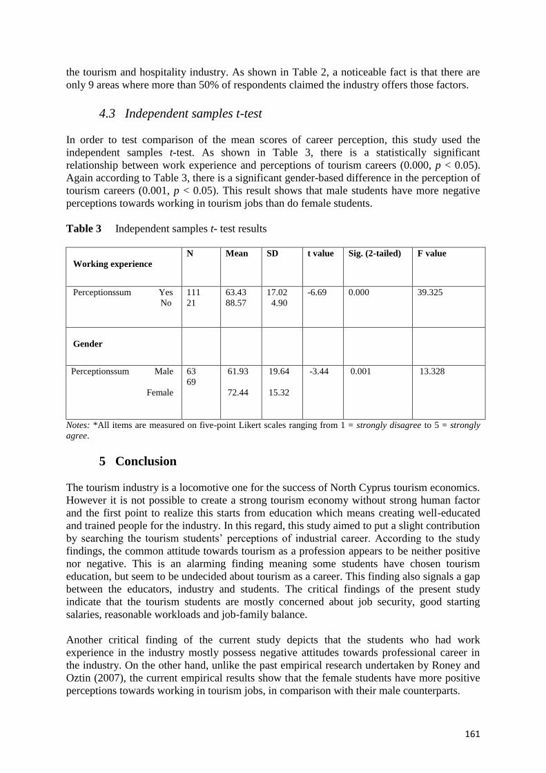
161

the tourism and hospitality industry. As shown in Table 2, a noticeable fact is that there are

only 9 areas where more than 50% of respondents claimed the industry offers those factors.

4.3 Independent samples t-test

In order to test comparison of the mean scores of career perception, this study used the

independent samples t-test. As shown in Table 3, there is a statistically significant

relationship between work experience and perceptions of tourism careers (0.000, p < 0.05).

Again according to Table 3, there is a significant gender-based difference in the perception of

tourism careers (0.001, p < 0.05). This result shows that male students have more negative

perceptions towards working in tourism jobs than do female students.

Table 3 Independent samples t- test results

Working experience

N Mean SD t value Sig. (2-tailed) F value

Perceptionssum Yes

No

111

21

63.43

88.57

17.02

4.90

-6.69

0.000

39.325

Gender

Perceptionssum Male

Female

63

69

61.93

72.44

19.64

15.32

-3.44

0.001 13.328

Notes: *All items are measured on five-point Likert scales ranging from 1 = strongly disagree to 5 = strongly

agree.

5 Conclusion

The tourism industry is a locomotive one for the success of North Cyprus tourism economics.

However it is not possible to create a strong tourism economy without strong human factor

and the first point to realize this starts from education which means creating well-educated

and trained people for the industry. In this regard, this study aimed to put a slight contribution

by searching the tourism students’ perceptions of industrial career. According to the study

findings, the common attitude towards tourism as a profession appears to be neither positive

nor negative. This is an alarming finding meaning some students have chosen tourism

education, but seem to be undecided about tourism as a career. This finding also signals a gap

between the educators, industry and students. The critical findings of the present study

indicate that the tourism students are mostly concerned about job security, good starting

salaries, reasonable workloads and job-family balance.

Another critical finding of the current study depicts that the students who had work

experience in the industry mostly possess negative attitudes towards professional career in

the industry. On the other hand, unlike the past empirical research undertaken by Roney and

Oztin (2007), the current empirical results show that the female students have more positive

perceptions towards working in tourism jobs, in comparison with their male counterparts.

162

Importantly, the critical finding from this study is the number of tourism students who have

no future plans towards getting a tourism profession. More than quarter of them is not willing

to work in the industry. Northern Cyprus is an island country dependent on tourism industrial

economy where there is already shortage of qualified people. Under the circumstances, the

industry should not have a chance to lose more than 40% of its qualified graduates.

The findings of this research study depict that more than 40% of the tourism students from

the universities of Northern Cyprus are not willing to work in the industry; an industry that

urgently needs well-educated and skilled personnel. This means the industry will lose more

than one-third of qualified graduates. Therefore, industry practitioners and tourism educators

should cooperatively deal with these problems as soon as possible if they want to improve the

service quality of Northern Cyprus as a destination brand. The tertiary tourism educators,

starting from the first year of education, should balance the theoretical education and training

at a rate of 50% and 50%.

Tourism students should certainly become professionalized according to their occupational

preferences such as travel agency, marketing, catering, and so forth. Through rotations in

different branches, their skills and capabilities should be observed and directed accordingly.

Standardized working conditions for trainees should be provided by the industry practitioners

and all these training periods should be under the routine control of tourism educators. After

a long period of training, new graduates will be ready to take managerial positions.

A rotational system in intensive customer-oriented areas can be improved for working days

such that a group of employees may alternately not work at the weekends by working ten

hours in the weekdays. Thus, this kind of managerial perspectives always undermine the

image of the industry. Like all research, the present study has also some limitations. First, the

study is based on a sample of students from Northern Cyprus universities and cannot be

generalized to other countries. Empirical studies may be conducted in other places in order to

find out current career perceptions and expectations of tourism students. More in-depth

studies, possibly qualitative in nature, are needed to ponder the unrevealed reasons and

aspects of career perceptions and expectations. Third, as a sample selection, this study

included the last year tourism students in the survey. This is also a limitation and future

studies could look at other levels of tourism and hospitality students.

References

1. Aksu, A. A. and Koksal, C. D. (2005). Perceptions and attitudes of tourism students in

Turkey. International Journal of Contemporary Hospitality Management, Vol.17, No.

5, pp.436–447.

2. Alipour, H. and Kilic, H. (2005). An institutional appraisal of tourism development

and planning: The case of the Turkish Republic of Northern Cyprus (TRNC). Journal

of Tourism Management, Vol. 26, No. 1, pp.79–94.

3. Arasli, H., Bavik, A. and Ekiz, H. E. (2006). The effects of nepotism on HRM and

psychological outcomes: The case of 3, 4, and 5 star hotels in Northern Cyprus.

International Journal of Sociology and Social Policy, Vol. 26, No. 7/8, pp.295–308.

163

4. Arasli, H. and Karadal, H. (2009). Impacts of superior politics on frontline

employees’ behavioral and psychological outcomes. Social Behavior and Personality,

Vol. 37, No. 2, pp.175–190.

5. Barclay, D.W., Thompson, R. and Higgins, C. (1995). The partial least squares (PLS)

approach to causal modeling: Personal computer adoption and use an illustration.

Technology Studies, Vol. 2, No. 2, pp. 285–309.

6. Barron, P., Maxwell, G., Broadbridge, A. and Ogden, S. (2007). Careers in hospitality

management: Generation Y’s experiences and perceptions. Journal of Hospitality and

Tourism Management, Vol. 14, No. 2, pp. 119–128.

7. Bates, T. (1990). Entrepreneur human capital inputs in small business longevity.

Review Economic Statistics, Vol. 72, No. 40, pp.551–559.

8. Baum, T. (2006). Human resource management for tourism, hospitality and leisure:

An international perspective, London: Thomson Learning.

9. Baum, T. (2007). Human resources in tourism: Still waiting for change. Tourism

Management, Vol. 28, No. 6, pp.1383–1399.

10. Baum, T., Amoah, V. and Spivack, S. (1997). Policy dimensions of human resource

management in the tourism and hospitality industries. International Journal of

Contemporary Hospitality Management, Vol. 9, No. 5/6, pp.221–229.

11. Birdir, B. (2002). Turizm ve otel isletmeciliği eğitimi alan lisans öğrencilerinin turizm

endüstrisinde çalısmayı tercih etmemelerinin temel nedenleri: Bir nominal grup

tekniği arastırması. In Ministry of Tourism (ed.), Proceedings of the conference and

workshop on tourism education, 495-504. Ankara: Ministry of Tourism Press.

12. Brien, A. (2004). Do I want a job in hospitality? Only till I get a real job! In K. A.

Smith & C. Schott (Eds.), Proceedings of the New Zealand Tourism and Hospitality

Research Conference (pp. 35–42). New Zealand: Victoria University of Wellington.

13. Choy, D. J. L. (1995). The quality of tourism employment. Tourism Management,

Vol. 16, No. 2, pp.129–137.

14. Christensen Hughes, J. M. (2002). Recruitment and selection issues and strategies

within international resort communities. In N. D'Annunzio-Green, G. A. Maxwell &

S. Watson (Eds.), Human Resource Management: International Perspective in

Hospitality and Tourism. London: Continuum.

164

15. Cooper, A., Gimeno-Gascon, F. and Woo, C. (1994). Initial human and financial

capital as predictors of new venture performance. Journal of Business Venturing, Vol.

9, No. 5, pp. 371–395.

16. Daskin, M. (2013). Favouritism and self-efficacy as antecedents on managers' politics

perceptions and job stress. Anatolia: An International Journal of Tourism and

Hospitality Research, Vol. 24, No. 3, pp.452–467.

http://dx.doi.org/10.1080/13032917.2013.807396.

17. Deery, M. and Shaw, R. (1999). An investigation of the relationship between

employee turnover and organizational culture. Journal of Hospitality & Tourism

Research, Vol. 23, No. 4, pp.387–400.

18. Field, A. (2000) Discovering Statistics using SPSS for Windows, London – Thousand

Oaks – New Delhi: Sage publications

19. Fornell, C. and Larcker, D.F. (1981). Evaluating structural equation models with

unobservable and measurement error. Journal of Marketing Research, Vol. 18, No. 1,

pp.39–50.

20. Freeland, B. (2000). Demands of training: Australian tourism and hospitality.

Adelaide, Australia: National Centre for Vocational Education Research.

21. Getz, D. (1994). Students' work experiences, perceptions and attitudes towards

careers in hospitality and tourism: a longitudinal case study in Spey Valley, Scotland.

International Journal of Hospitality Management, Vol. 13, No.1, pp.25–37.

22. Gu, H., Kavanaugh, R. R. and Cong, Y. (2007). Empirical studies of tourism

education in China. Journal of Teaching in Travel & Tourism, Vol. 7, No. 1, pp.3–24.

23. Horner, S. and Swarbrooke, J. (2004). International cases in tourism management:

Case 26 Tourism education and training (pp. 261-273). London: Elsevier

Butterworth Heinemann.

24. Jenkins, A. K. (2001). Making a career of it? Hospitality students’ future

perspectives: an Anglo-Dutch study. International Journal of Contemporary

Hospitality Management, Vol. 13, No. 1, pp.13–20.

25. Kangasharju, A. and Pekkala, S. (2002). The role of education and self-employment

success in Finland. Growth and Change, Vol. 33, No. 2, pp.216–37.

26. Kelley-Patterson, D. and George, C. (2001). Securing graduate commitment: an

exploration of the comparative expectations of placement students, graduate recruits

http://dx.doi.org/10.1080/13032917.2013.807396

165

and human resource managers within the hospitality, leisure and tourism industries.

International Journal of Hospitality Management, Vol. 20, No. 4, pp.311–323.

27. Kusluvan, S. and Kusluvan, Z. (2000). Perceptions and attitudes of undergraduate

tourism students towards working in the tourism industry in Turkey. Tourism

Management, Vol. 21, No. 3, pp.251–269.

28. Kusluvan, S., Kusluvan, Z., Ilhan, Z. and Buyruk, L. (2010). The human dimension: a

review of human resources management issues in the tourism and hospitality industry.

Cornell Hospitality Quarterly, Vol. 51, No. 2, pp.171–214.

29. Kyriacou, C. and Coulthard, M. (2000). Undergraduates’ views of teaching as a career

choice. Journal of Education for Teaching, Vol. 26, No. 2, pp.117–126.

30. Lent, R. W., Brown, S. D. and Hackett, G. (1994). Toward a unifying social cognitive

theory of career and academic interest, choice, and performance [Monograph].

Journal of Vocational Behavior, Vol. 45, No. 1, pp.79–122.

31. Lewis, A. and Airey, D. (2001). Tourism careers in Trinidad and Tobago: Perceptions

of secondary school students. Tourism and Hospitality Research, Vol. 3, No. 1, pp.7–

20.

32. Lucas, R. and Jeffries, L. (1991). The demographic 'timebomb' and how some

hospitality employers are responding to the challenge. International Journal of

Hospitality Management, Vol. 10, No. 4, pp.323–337.

33. Nunnally, J. C. (1978). Psychometric theory (2nd Ed.). New York: McGraw-Hill

Book Company.

34. Pavesic, D. V. and Brymer, R. A. (1990). Job satisfaction: What’s happening to the

young managers? Cornell Hotel and Restaurant Administration Quarterly, Vol. 31,

No. 1, pp.90–96.

35. Pennings, L., Lee, K. and van Wittteloostuijn, A. (1998). Human capital, social

capital and firm dissolution. Academy of Management Journal, Vol. 41, pp.425–440.

36. Pizam, A. (1982). Tourism manpower: the state of the art. Journal of Travel research,

Vol. 11, No. 2, pp.5–9.

37. Richardson, S. (2008). Undergraduate tourism and hospitality students attitudes

toward a career in the industry: A Preliminary Investigation. Journal of Teaching in

Travel & Tourism, Vol. 8, No. 1, pp.23–46.

166

38. Richardson, S. (2009). Undergraduates’ perceptions of tourism and hospitality as a

career choice. International Journal of Hospitality Management, Vol. 28, No. 3,

pp.382–388.

39. Richardson, S. (2010). Generation Y's Perceptions and Attitudes Towards a Career in

Tourism and Hospitality. Journal of Human Resources in Hospitality & Tourism, Vol.

9, No. 2, pp.179–199.

40. Richardson, S. and Butler, G. (2012). Attitudes of Malaysian Tourism and Hospitality

Students' towards a Career in the Industry. Asia Pacific Journal of Tourism Research,

Vol. 17, No. 3, pp.262 –276.

41. Roney, A. and Oztin, P. (2007). Career Perceptions of Undergraduate Tourism

Students: A Case Study in Turkey. Journal of Hospitality, Leisure, Sport and Tourism

Education, Vol. 6, No. 1, pp.4–17.

42. Schultz, T.W. (1971). Investment in Human Capital. New York. The Free Press.

43. Sigala, M. and Baum T. (2003). Trends and issues in tourism and hospitality higher

education: Visioning the future. Tourism and Hospitality Research, Vol. 4, No. 4,

pp.367–376.

44. Travel Trade Gazette (2000). Poor image puts off recruits, TTG, Travel Trade

Gazette, U.K. and Ireland, 31.

45. Wan, Y.K.P. (2010). Exploratory assessment of the Macao casino dealers’ job

perceptions. International Journal of Hospitality Management, Vol. 29, No. 1, pp.62–

71.

46. WTTC (2002). HR Opportunities and Challenge. A Report by the WTTC Human

Resource Task Force (Publication no. www.wttc.org/publications) from World Travel

and Tourism Council (WTTC).

47. World Travel & Tourism Council (2012). Economic Data Search Tool.

http://www.wttc.org.

167

THE EFFECT OF FOREIGN BANK ENTRY ON THE FINANCIAL

PERFORMANCE OF THE COMMERCIAL BANKS IN TURKEY

Ayhan Kapusuzoglu

Ankara Yildirim Beyazit University, Turkey

E-mail: [email protected]

Nildag Basak Ceylan

Ankara Yildirim Beyazit University, Turkey


Abstract

Due to the globalization and financial market integration, the investors are more fascinated to

make their investments to foreign countries where there are opportunities. In this sense, the

purpose of this study is to analyze the effect of foreign banks’ entry on the commercial

banks’ financial performance participating in the domestic financial market for the case of

Turkey. Our analysis are carried out for the period 2003:01- 2013:04 and the data used in the

study are quarterly. In the analysis, 33 commercial banks are included in the study. As a

model Ordinary Leat Square (OLS) method is used. The main findings of the study suggest

that foreign bank entry increases loss reserve measured as loss reserve / total gross loans,

maturity mismatch and decreases non performing loan of the commercial banks.

Keywords: Bank performance, foreign bank entry, OLS

1. Introduction

Owing to the globalization, foreign banks’ interest in entering into the local economies has

increased. There may be many reasons of these foreign banks entering into the other

countries domestic markets. This may be because of they facilitate their trading activiries.

The positive and negative impacts of of these entries are also reported in several studies.

Levine (1996), Walter and Gray (1983), Gelb and Sagari (1990) reported the potential gains

of the domestic economy in the case a foreign bank enters to the market. Detragiache, Tressel

and Gupta (2008) reported that in low-income countries the entry of foreign banks is

relationed with less credit being extended. Kalluru and Sham (2009) examined how foreign

bank entry affected the public sector banks in India and reported that it increased

profitability, overhead expenses and non performing loans. Boadi (2015) analyzed the impact

of foreign bank entry on the performance of domestic banks in Ghana for the period 1997-

2014. The results show that it increased net interest income and return on assets. Opposing to

their finding, Claessens, Demirguc-Kunt, and Huizinga (2001) found that foreign banks entry

decreases the profitability and margins of the banks in domestic market.

In this paper, the effect of foreign banks entry on the financial performance of commercial

banks are examined for the case of Turkey in terms of business orientation, efficiency, asset

quality and stability.



168

The paper is organized as follows: In the second section data and methodology is presented

and the last section concludes.


In the study, the period that is considered is between 2003:01-2013:04 and the data are

quarterly. The data on banks are obtained from Banks Association of Turkey, Borsa Istanbul,

Independent Audit Reports and Bankscope. In our dataset, 33 banks are included. Although

as of December 2013, 50 banks are operating in Turkey, 17 of them are excluded. This is

because either the data of the banks do not go back long enough, or transferred to the Savings

Deposit Insurance Fund or Islamic banks.

We consider a set of variables to consider the effect of foreign bank entry on the commercial

banks, denoted as Yi,t, which are fee income/total operational income, non-deposit-

funding/total funding, loans to deposits ratio, cost to income ratio, overheads/total assets,

loan loss reserves/total gross loans, loan loss provisions to total gross loans, non-performing

loans to total gross loans, maturity match, z-score, return on assets, equity to assets ratio,

total assets (in logarithm), fixed assets/total assets. D denotes the foreign bank entry. In the

case of a foreign bank entry exist in a particular date, 1 was assigned to the related term

(quarter), otherwise 0 was assigned.

To be specific the following OLS model is estimated:

ti,1,

ftiDaY

The bank efficiency variables are; overhead cost (operating cost/total costs), cost/income. For

the asset quality, loss reserves/gross loans, loan loss provisions/gross loans and non-

performing loans/gross loans are taken. Loan loss provision is obtained by dividing loan loss

provisions to net interest income which shows the quality of asset of a bank. When quality of

the assets are not good, the negative affect is expected on the profitability of the banks. For

the bank stability, maturity match (liquid asset/deposit and short term funding), z-score (the

summation of return on assets and capital to asset ratio to standard deviation of return on

assets) variables are used. The high z-score shows that the bank is stable and far from

insolvency.

3. Conclusion

The empirical results of the OLS shows that foreign bank entry increases loss reserve

measured as loss reserve / total gross loans where the statistically significant effect is not

found in the study of Claessens, Demirguc-Kunt, and Huizinga (1998); increases maturity

mismatch and decreases non performing loan of the commercial banks in the domestic

market opposing to the study of Ukaegbu (2014) who reported in his study that, foreign

banks enteries increases non performing loans of the domestic banks.

169

References:

1. Boadi, I. (2015). “Effects of Foreign Banks Entry on the Operations of Domestic

Banks-Empirical Evidence from Ghana”. International Journal of Business and

Management, 10 (12).

2. Claessens, S., A. Demirguc-Kunt, and H. Huizinga (2001). “How does foreign entry

affect domestic banking markets?”. Journal of Banking and Finance, 25, 891-911.

3. Claessens, S., A. Demirguc-Kunt, and H. Huizinga (1998). “How does foreign entry

affect the domestic banking market?”. Working Paper, World Bank.

4. Detragiache, E., P. Gupta, and T. Tressel (2008). “Foreign banks in poor countries:

Theory and evidence”. Journal of Finance, 63, 2123-2160.

5. Gelb, A., and S. Sagari (1990). Banking, in P. Messerlin and K. Sanvant, eds., The

Uruguay Round: Services in the World Economy. Washington, D.C.: The World

Bank and UN Centre on Transnational Corporations.

6. Kalluru, S. R. and B. K. Sham (2009).“Does foreign bank entry affect operations of

domestic banks? A study on Indian public sector banks”. IUP Journal of Managerial

Economics, 7.3/4 (Aug-Nov 2009), 40-51.

7. Levine, R. (1996). “Foreign banks, financial development, and economic growth”, in

Claude E. Barfield, ed., International Financial Markets. Washington, D.C., AEI

Press.

8. Ukaegbu, B. (2014). “The impact of foreign bank entry on domestic banking in a

developing country: The Kenyan perspective”. Banks and Bank Systems, 9 (1), 28-35.

9. Walter, I., and H. P. Gray (1983). “Protectionism, and international banking, Sectoral

efficiency, competitive structure and national policy”. Journal of Banking and

Finance, 7, 597-609.

170

THE DEVELOPMENT OF E-COMMERCE AND THE INFLUENCE OF

CONSUMER CONFIDENCE ON THE ECONOMY OF IRAN

Panteha Farmanesh


The electronic era of commerce is a fundamental and vital part of businesses worldwide. The

explosion of E-commerce has generated a vast array of opportunities for businesses to thrive,

utilising the ability to pass information electronically.

The exploitation by businesses of this method of conducting commercial transactions has

established a core business practise allowing companies to conduct their business in this

Dot.Com age. However, these practises are not prevalent with in The Islamic Republic of

Iran due to the compulsory government restrictions and the external sanctions enforced by the

remainder of the world. This study has explored the influential factors that have prevented the

enhancement of consumer confidence within Iran however the growth of e-commerce

although sporadic has not been allowed to flourish.

The restrictions that are currently affecting Iran are inhibiting the development of an e-

commerce industry that in turn is restricting the economy of both corporations and the

country. In this research, the author has highlighted the effects that the restrictions imposed

on the e-commerce and e-marketing sectors could, if removed or loosened, dramatically

improve the economics of Iran. The potential technological advancements in Iran are vast,

and the result of this study indicates that consumer confidence within e-commerce, if

permitted to thrive could generate a huge impetus with the economy of Iran.

Keywords: electronic commerce; consumer confidence, data security; Iran

1. Introduction

The dramatic increase in internet and the detonation of its usage have facilitated the

development of electronic commerce which is described as the movement of buying and

selling, or the trading of products, service and information between and among the

organizations and individuals all the way through computer networks including the internet.

When investing in online/internet marketing, strategic thinking will bring to the best rewards.

From the very inception of the Internet and the World Wide Web, the effect that has been felt

on companies and corporations around the globe has transformed the running and functions

of operating businesses. In terms of the most dramatic change, the marketing process has

been the most influenced with companies now regularly using this new form of technology to

manage their businesses and to develop new areas of expertise. With the generation of the

information technology age, the utilization of the Internet has effectively increased business

in companies and developed a new education process. By using the internet consumers from

around the world are able to engage in cross global enterprise and experience a marketplace

that has no geographical borders with the additional benefit of having no time constraints. By

using an e-commerce strategy there is the opportunity to provide and exploit a complete

marketing capability.

171

The companies that thrive with in this new marketplace are those that is able to analyze and

react to the strengths and weaknesses of communities and other companies. To recognize the

information available to them from across the Internet and to respond in a manner that suits

the consumer via an e-commerce approach. The design and implementation of such

opportunities will then be employed to then extend their competencies and use a variety of

marketing options at their disposal e.g. direct marketing, transaction marketing and email

marketing. All of these opportunities have been created from the development of the Internet

and the World Wide Web.

2. Literature review

2.1 The definition of e-commerce

According to Different definitions have been suggested to describe electronic commerce and

the vast majority is based upon previous experiences of utilizing electronic commerce

(Bonyani, 2014). The European Commission stated in 1997 that electronic commerce was the

“process and transmitting of electronic data including text, voice and image. Electronic

commerce embraces various activities such as electronic transaction of goods and services,

immediate delivery of digital demands, electronic payment, electronic stock exchange,

electronic bill of lading, commercial plans, direct marketing and after sales services.”

2.2 Islamic law and e-commerce

According to my recent research into Islamic law, it was apparent that the Quran was a key

factor in the preparation by the lawmakers. All those who approach the topic of Islamic Law

enter an area that cannot be easily compared to a western counterpart, as much of the laws of

Islamic countries including Iran are governed by decrees set down by the Prophet. For

example at the time of the Prophet, he specifically permitted some merchants to act in one

way whereas others he strictly forbade. Therefore from my research current laws directly

affected by those set down by the Prophet. As a result those sacred directions have provided

specific guidelines from which to work within, however that have allowed a very constricted

range for interpretation. Therefore the current lawmakers and legislators have a very limited

source from which to apply their rules.

2.3 The Internet and e-commerce in Iran

The Iranian society has only recently experienced the opportunity of conducting electronic

commerce and therefore has had limited experience of legislative processes to protect

consumers. The legislation in relation to e-commerce was accepted and introduced by the

Iranian Parliament (Majlis) on 7th January 2004, comprising of 81 articles designed

specifically to align the Iranian development of e-commerce with that of global and domestic

requirements (Mancuso, 2007). The laws comprised of six defining chapters on the subject of

data exchange via digital/computer networks, which at the time was considered to be new

technology.

Within the third subdivision of this law, data protection is introduced with a number of

provisions, which are set down in three defining areas. These are highlighted as the

following:

• The ability to have access to complete information

• The right of removal of personal data

172

• The ability to protect oneself from prejudicial contractual obligations

2.4 Situation of e-commerce in Iran

As a fledgling country in terms of the electronic commerce arena, Iran faces a lengthy road to

reach what most would consider to an acceptable level. With the entry of the new technology

into this field, it has raised new requirements in data processing, the interchange of

information and the necessity for the proper tools and infrastructures for its implementation.

However, in Iran the main users of Internet are researchers in universities and specially

designed centers in various cities however their access has a limited level.

In order to develop electronic commerce in the country and to enable the entry in the global

market places and organizations such as the World Trade Organization, the country must first

create a stable and efficient banking system (Najafi 2010). So, by using the information and

communication technology it is vital for the creation of electronic banking and then to

integrate it with the existing banking system, makes this a massive task. Although over the

years some methods of providing electronic banking services such as ATM machines and

debit cards in the banking system of the country have been implemented, there is still a long

way to go to achieve the level of electronic banking in the developed countries.

2.5 Consumer confidence in Iran

Under the current regulations offered to protect consumers the legal system is divided in to

two areas of protection.

1. Specific legislation – these are laws and regulations that have been

reviewed and passed by the Majlis

2. Research Centres – designed to encourage progressive approach to

review existing and create new legislation for review and enforcement by

the government.

Consumers today however remain cautious and in some cases unprotected from the

unscrupulous merchants, hence these policies are under continual review. As a result of these

developments the consumers are discovering a wider array of products and facilities in the

global market. It appears that as countries develop merchandises from outside markets are

actively encouraged therefore creating an ideal opportunity for countries wishing to export

their produce (Ranjbarian et al. 2011). In countries developing like Iran, this is actively

encouraged too, together with regulations to improve the development of home based

industries to compliment the arrival of the vast array of foreign products. With respect to

precedents set with in e-commerce law, there are very few examples to enable the legislators

of law to create a suitable framework from which to work within. The essence of an

electronic contract are essentially set down that the parties to the contract are not required to

be present however their acceptance can be verified by simply receiving electronic

confirmation. This is essentially the same for e-payments, where the funds are not physically

passed between parties, but by the transference of funds by electronic means either via credit

card payment or through e-banking transferring (Haghighi et al. 2014). The most important

infrastructures are namely appropriate communication and telecommunication networks, data

interchange security, proper legal infrastructures, cultural readiness of the society and

enterprises for accepting and using electronic banking services.

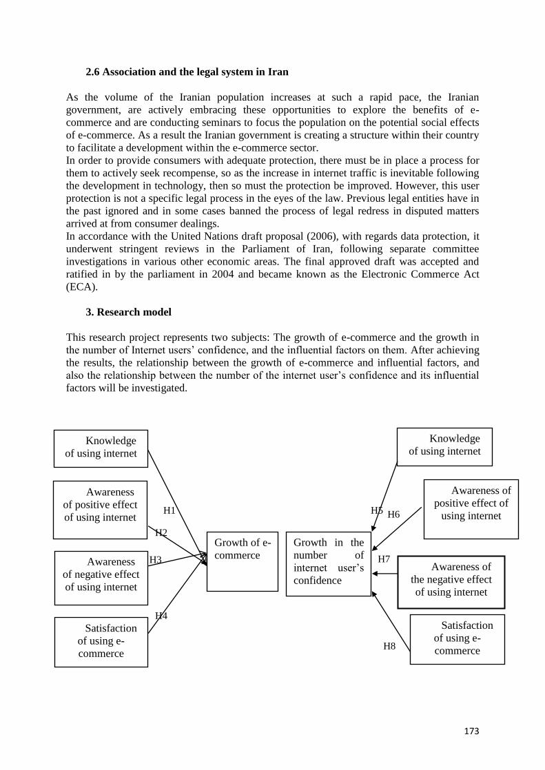
173

2.6 Association and the legal system in Iran

As the volume of the Iranian population increases at such a rapid pace, the Iranian

government, are actively embracing these opportunities to explore the benefits of e-

commerce and are conducting seminars to focus the population on the potential social effects

of e-commerce. As a result the Iranian government is creating a structure within their country

to facilitate a development within the e-commerce sector.

In order to provide consumers with adequate protection, there must be in place a process for

them to actively seek recompense, so as the increase in internet traffic is inevitable following

the development in technology, then so must the protection be improved. However, this user

protection is not a specific legal process in the eyes of the law. Previous legal entities have in

the past ignored and in some cases banned the process of legal redress in disputed matters

arrived at from consumer dealings.

In accordance with the United Nations draft proposal (2006), with regards data protection, it

underwent stringent reviews in the Parliament of Iran, following separate committee

investigations in various other economic areas. The final approved draft was accepted and

ratified in by the parliament in 2004 and became known as the Electronic Commerce Act

(ECA).

3. Research model

This research project represents two subjects: The growth of e-commerce and the growth in

the number of Internet users’ confidence, and the influential factors on them. After achieving

the results, the relationship between the growth of e-commerce and influential factors, and

also the relationship between the number of the internet user’s confidence and its influential

factors will be investigated.

Satisfaction

of using e-

commerce

Awareness

of negative effect

of using internet

Knowledge

of using internet

Satisfaction

of using e-

commerce

Awareness

of positive effect

of using internet

Growth of e-

commerce

Growth in the

number of

internet user’s

confidence

Knowledge

of using internet

Awareness of

positive effect of

using internet H1

H2

H3

H4

H5 H6

H

7

Awareness of

the negative effect

of using internet

H8

H7

174

3.1 Research Hypothesis

For considering the impact of four factors, influential on growth of e-commerce in Iran, the

following hypotheses are tested.

H1: There is a significant relationship between the knowledge of using the Internet and the

growth of e-commerce in Iran.

H2: There is a significant relationship between the awareness of the positive effect of using

the Internet and growth of e-commerce in Iran.

H3: There is a significant relationship between the awareness of the negative effect of using

the Internet and the growth of e-commerce in Iran.

H4: There is a significant relationship between the satisfaction of using e-commerce and the


For considering the impact of the four factors on consumer confidence within e-commerce

the following hypotheses are tested.

H5: There is a significant relationship between the knowledge of using the Internet and the

growth in number of Internet users’ confidence in Iran.


the Internet and the growth in the number of Internet users’ confidence in Iran.


the Internet and the growth in the number of Internet users’ confidence in Iran.


growth in the number of Internet users’ confidence in Iran.

3.2 Methodology

In this research, the author used a self-administrated questionnaire method of delivery and

collection of data from participants, with the questions being designed to collect data on

respondents’ attitude. A survey was conducted on 171 respondents in order to explore the

issues that arise in relation to consumer confidence and effect on the growth of e-commerce.

Participants were chosen randomly in both male and female groups in order to answer

questions dealing with essentials of computer, Internet, and e-commerce.

The potential technological advancements in Iran are vast, and the result of this study

indicates that consumer confidence within e-commerce, if permitted to thrive could generate

a huge impetus with the economy of Iran.

3.3 Research Sample

In this research the population of interest is Iranian people. The sampling method, which is

used in this study, is convenience sampling, based on the concept of random selection.

According to convenience sampling, which is a non-probability technique, the researcher is

able to use their judgment in order to verify the sample size. Since this study was applied

within just one place with a small population, plus due to lack of awareness of the

respondents about the research topic and limited time and budget, this researcher decided to

apply 200 questionnaires in order to generate a minimum required respondents. As a result a

selection of people at a popular mall in Tehran were chosen randomly to generate a wider

audience for the study to be tested on, to discover how they thought their involvement with

the internet and e-commerce would influence their confidence. Finally from these 200

questionnaires, 171 questionnaires were collected thereby creating the sample size which this

author considered adequate for this research.

175

4. Descriptive Analysis and result

To carry out this research 200 questionnaires were spread randomly among people from

whom 171 respondents replied. From the 171 total respondents, the breakdown of gender

responses was as follows: 45.6% were female and 54.5% were male.

The demographics of those respondents included the following; 15.2% were aged 19 or

under, 23.4% were aged between 20 and 24, 28.1% were aged between 25 and 30, and 33.3%

were aged 30 or more.

Gender

Frequenc

y Percent

Valid

Percent

Cumulative

Percent

Valid Male 93 54.4 54.4 54.4

Female 78 45.6 45.6 100.0

Total 171 100.0 100.0

Gender distribution

Age

Frequenc

y Percent

Valid

Percent

Cumulative

Percent

Valid 19 or under 26 15.2 15.2 15.2

20-24 40 23.4 23.4 38.6

25-30 48 28.1 28.1 66.7

30 and more 57 33.3 33.3 100.0

Total 171 100.0 100.0

Age distribution

Computer

Frequenc

y Percent

Valid

Percent

Cumulative

Percent

Valid yes 158 92.4 92.4 92.4

No 13 7.6 7.6 100.0

Total 171 100.0 100.0

Accessibility to computer

Internet

Frequenc

y Percent

Valid

Percent

Cumulative

Percent

Valid Yes 150 87.7 87.7 87.7

No 21 12.3 12.3 100.0

Total 171 100.0 100.0

Accessibility to the internet

176

Used

Frequenc

y Percent

Valid

Percent

Cumulative

Percent

Valid Yes 134 78.4 78.4 78.4

No 37 21.6 21.6 100.0

Total 171 100.0 100.0

Used internet before

Ecommerce

Frequenc

y Percent

Valid

Percent

Cumulative

Percent

Valid Yes 88 51.5 51.5 51.5

No 83 48.5 48.5 100.0

Total 171 100.0 100.0

Use e-commerce

4.1 The result of factor analysis

According to table below, the result of KMO for growth of e-commerce and consumer

confidence is 0.616 which is satisfactory and from Bartlett’s test is significant at level 0.000.

KMO and Bartlett's Test

Kaiser-Meyer-Olkin Measure of Sampling

Adequacy.

.616

Bartlett's Test of

Sphericity

Approx. Chi-Square 212.306

Df 21

Sig. .000

Table below as a descriptive analysis which consisted of 34 items:

These items represent the questions from the questionnaire, which is followed by likert scale

questionnaire.

IM: Knowledge of using the internet

PF: The awareness of the positive effect of using the internet

NF: The awareness of the negative effect of using the internet

SA: The satisfaction of using the internet

177

Descriptive Statistics

Mean

Std.

Deviation

Analysis

N

IM1 3.75 1.217 171

IM2 4.33 .797 171

IM3 4.29 .709 171

IM4 4.28 .883 171

IM5 3.70 .963 171

IM6 3.77 1.052 171

IM7 3.54 .989 171

IM8 3.40 .898 171

IM9 3.09 .963 171

IM10 3.87 .901 171

IM11 3.80 1.015 171

IM12 4.09 1.144 171

IM13 4.26 .918 171

PF1 4.50 .672 171

PF2 4.42 .658 171

PF3 4.39 .671 171

PF4 3.89 .836 171

PF5 3.92 .982 171

PF6 3.79 .941 171

NF1 3.81 1.101 171

NF2 3.97 .904 171

NF3 4.25 1.073 171

NF4 3.67 1.006 171

NF5 4.06 1.044 171

NF6 3.87 .924 171

NF7 3.93 .878 171

SA1 3.14 1.303 171

SA2 2.80 1.111 171

SA3 4.27 .742 171

SA4 4.06 .780 171

SA5 4.16 .822 171

SA6 4.19 .821 171

SA7 4.32 .771 171

SA8 3.99 .748 171

Descriptive analysis of all items

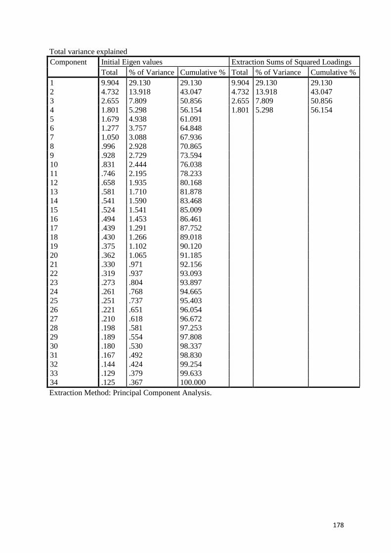
178

Total variance explained

Component Initial Eigen values Extraction Sums of Squared Loadings

Total % of Variance Cumulative % Total % of Variance Cumulative %

1 9.904 29.130 29.130 9.904 29.130 29.130

2 4.732 13.918 43.047 4.732 13.918 43.047

3 2.655 7.809 50.856 2.655 7.809 50.856

4 1.801 5.298 56.154 1.801 5.298 56.154

5 1.679 4.938 61.091

6 1.277 3.757 64.848

7 1.050 3.088 67.936

8 .996 2.928 70.865

9 .928 2.729 73.594

10 .831 2.444 76.038

11 .746 2.195 78.233

12 .658 1.935 80.168

13 .581 1.710 81.878

14 .541 1.590 83.468

15 .524 1.541 85.009

16 .494 1.453 86.461

17 .439 1.291 87.752

18 .430 1.266 89.018

19 .375 1.102 90.120

20 .362 1.065 91.185

21 .330 .971 92.156

22 .319 .937 93.093

23 .273 .804 93.897

24 .261 .768 94.665

25 .251 .737 95.403

26 .221 .651 96.054

27 .210 .618 96.672

28 .198 .581 97.253

29 .189 .554 97.808

30 .180 .530 98.337

31 .167 .492 98.830

32 .144 .424 99.254

33 .129 .379 99.633

34 .125 .367 100.000

Extraction Method: Principal Component Analysis.

179

KMO and Bartlett's Test

Kaiser-Meyer-Olkin Measure of Sampling

Adequacy.

.868

Bartlett's Test of

Sphericity

Approx. Chi-Square 3650.040

Df 561

Sig. .000

KMO and Bartlett’s test for IK, PE, NE, SA

KMO table which is Rotated component matrix, also shows that contrary to the original

model, the items of internet knowledge, positive effect of using internet, negative effect of

using internet, satisfaction of using e-commerce were loaded in to four components.

4.2 The results of correlation analysis

For considering the impact of four factors, influential on growth of e-marketing in Iran, the

following hypotheses are tested.

H1: There is a significant relationship between the knowledge of using the internet and the



the internet and growth of e-commerce in Iran.


the internet and the growth of e-commerce in Iran.



The result of correlation analysis for the above hypotheses is as follow:

According to the table 4.15, the correlation is significant at the 0.01 level for knowledge of

internet and growth of e-commerce. Therefore it can be concluded that H1 is accepted, in

other words, there is a significant relationship between the knowledge of the internet and the

growth of e-commerce in Iran. This demonstrates that the knowledge of internet will

positively influence the growth of e-commerce in Iran.

In table below, this shows that correlation is significant at the 0.01 level for positive effect of

using internet and growth of e-marketing, which means H2, is accepted and it can be

concluded that there is a positive effect that the using of the internet is effective in the growth

of e-commerce within Iran.

Correlations

Knowledge Growth

Knowledge Pearson

Correlation

1 .401**

Sig. (2-tailed) .000

N 171 171

Growth Pearson

Correlation

.401** 1


N 171 171

**. Correlation is significant at the 0.01 level (2-tailed).

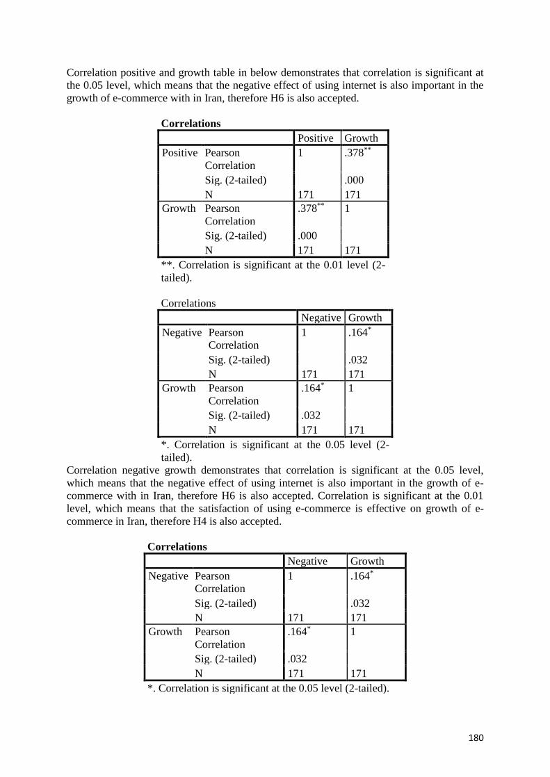
180

Correlation positive and growth table in below demonstrates that correlation is significant at

the 0.05 level, which means that the negative effect of using internet is also important in the

growth of e-commerce with in Iran, therefore H6 is also accepted.

Correlations

Positive Growth

Positive Pearson

Correlation

1 .378**


N 171 171

Growth Pearson

Correlation

.378** 1


N 171 171

**. Correlation is significant at the 0.01 level (2-

tailed).

Correlations

Negative Growth

Negative Pearson

Correlation

1 .164*


N 171 171

Growth Pearson

Correlation

.164* 1


N 171 171

*. Correlation is significant at the 0.05 level (2-

tailed).

Correlation negative growth demonstrates that correlation is significant at the 0.05 level,

which means that the negative effect of using internet is also important in the growth of e-

commerce with in Iran, therefore H6 is also accepted. Correlation is significant at the 0.01

level, which means that the satisfaction of using e-commerce is effective on growth of e-

commerce in Iran, therefore H4 is also accepted.

Correlations

Negative Growth

Negative Pearson

Correlation

1 .164*


N 171 171

Growth Pearson

Correlation

.164* 1


N 171 171

*. Correlation is significant at the 0.05 level (2-tailed).

181

Correlations

Satisfaction Growth

Satisfactio

n

Pearson

Correlation

1 .447**


N 171 171

Growth Pearson

Correlation

.447** 1


N 171 171


For considering the impact of the four factors on consumer confidence within e-commerce

the following hypotheses are tested.

H5: There is a significant relationship between the knowledge of using the internet and the

growth in number of internet users’ confidence in Iran.


the internet and the growth in the number of internet users’ confidence in Iran.


the internet and the growth in the number of internet users’ confidence in Iran.


growth in the number of internet users’ confidence in Iran. As presented in table 4.21, the

correlation for H5 is significant at the level 0.01. This therefore means H5 is accepted, in

other words, there is a significant relationship between the knowledge of using the internet

and consumer confidence within e-commerce in Iran.

According to table below, H6 is also accepted because the correlation is considered

significant at the 0.01 level, therefore the positive effects of using the internet impact on the

consumer confidence for the number of e-commerce users.

Correlations

Positive RULE

Positive Pearson

Correlation

1 .227**


N 171 171

RULE Pearson

Correlation

.227** 1


N 171 171

**. Correlation is significant at the 0.01 level (2-

tailed).

Table 4.23 shows that H7 is rejected in order to negative result, consequently the negative

effect of using internet has not been significant in relation to consumer confidence within e-

commerce.

182

Correlations

Negative RULE

Negative Pearson

Correlation

1 -.130-


N 171 171

RULE Pearson

Correlation

-.130- 1


N 171 171

Table below demonstrates, H8 is accepted, in order to correlation is significant at the 0.01

level, which means the satisfaction of using e-commerce can and will impact upon consumer

confidence.

Correlations

Satisfactio

n RULE

Satisfactio

n

Pearson

Correlation

1 .270**


N 171 171

RULE Pearson

Correlation

.270** 1


N 171 171


In order to study the relationship between these factors correlation analysis has been used and

regarding to the result of table 4.19 the calculated correlation is 0.447.

H4: According to H4, “There is a significant relationship between satisfaction of using e-

commerce and growth of e-marketing in Iran”. In order to study the relationship between

these factors correlation analysis has been used and regarding to the result of table 4.19 the

calculated correlation is 0.447.

Among these four variables, satisfaction of using e-commerce has the highest correlation

value of(0.447), followed by knowledge of the internet (0.401), awareness of positive effect

of using internet (0.378), the awareness of the negative effect of using internet (0.164).

In order for the author to demonstrate the co-relation between the satisfaction of using e-

commerce and the growth of e-marketing, it was established that the two aspects go hand in

hand. The element of trust in the e-commerce sector exists from the development of

legislation put in place to protect consumers. The development of such legislation has

confirmed that with more trust, consumers will inevitably feel more comfortable to use the e-

commerce and therefore develop e-business. With the improvements of data security in the e-

commerce field, the confidence in consumers will significantly grow and this in turn will

183

further improve the e-commerce sectors’ economy. To allow e-marketing to flourish, the data

security and the laws that cover it, should reflect the developing nature and thereby continue

to provide protection for consumers. This will allow a fledgling economy to increase and

therefore the country’s overall economy to improve as a result. In order to study the

relationship between these factors correlation analysis has been used and regarding to the

result of table 4.21 the calculated correlation is 0.377.

Among these four variables, knowledge of the internet has the highest correlation value

of(0.377), followed by satisfaction of using e-commerce (0.270), awareness of positive effect

of using internet (0.227), awareness of negative effect (0.164).

5. Conclusions and Recommendation

After the Factor Analysis, it was discovered that three of the indicators were found not to be

important on the growth of e-marketing and the growth of consumer confidence within e-

commerce. However, we have retained them (albeit they have not had any effect on the

result) in order to utilize them for correlation analysis.

5.1 Conclusions

H1: “There is a significant relationship between the knowledge of using the internet and the

growth of e-commerce in Iran”.

Consumer awareness of the uses of the internet and how it can affect their lives is a crucial

aspect for the development of the e-commerce sector. The knowledge and the personal

understanding of how the internet can positively affect personal development through

education, personal research and a wide range of facilities offers the user the opportunity to

explore a wide array of options. It is this awareness that is offering e-commerce a prospect of

establishing a true growth in business opportunities. By providing consumers with the ability

of understanding and being reassured by their knowledge, it is expected that consumers will

be able thrive and therefore the e-marketing sector alongside.

H2: “There is a significant relationship between the awareness of the positive effect of using

the internet and the growth of e-commerce in Iran”.

The use of the internet and the positive affect it can generate in consumers lives can be

highlighted in many ways, including accessing information previously unavailable at ones

fingertips, the speed of finding out data and the benefit of discovering more facilities

available. It is this kind of immediate response time that allows consumers to provide

themselves with up to date information thereby allowing e-marketing opportunities for

corporations to investigate. Therefore this is allowing a significant growth in e-marketing

prospects and enabling businesses to thrive on the consumers’ knowledge and understanding.

H3: “There is a significant relationship between the awareness of the negative effect of using

the internet and the growth of e-commerce in Iran”.

Consumer knowledge of the reverse side of the internet comes in many forms. Consumers are

constantly being advised of the affects third parties accessing their personal data can have on

them. The comparative high cost of accessing the internet and the poor connectivity which

leads to the frustrations of delayed responses together with the underlying fear factor leads to

a negative effect on the use of the internet. These concerns are inevitably hindering the

184

development of e-marketing prospects. Plus if one considers that e-marketing also generates

junk mail/spam, the effects are therefore magnified still further. However the main and most

relevant concern remains the constant threat of security breaches which prevents many from

engaging in e-commerce.

H5: “There is a relationship between the knowledge of the internet and the growth in number

of the internet user’s confidence in Iran”.

In order to generate an improved e-commercial environment the knowledge and training

available to consumers will enhance the opportunities of increasing electronic business. It is

the awareness of what the internet is capable of providing to individuals and companies alike

that makes it so essential. The speed and access to data has enabled consumers to explore and

refine their research capabilities. With this understanding of the internet comes a greater

understanding subject to the availability of legislative protection. Should the government of

Iran establish sustainable data protection legislation, therefore the prospect of improving e-

commerce will be even greater.

H6: “There is a relationship between the awareness of the positive affect of using the internet

and the growth in number of internet user’s confidence in Iran”.

The awareness of the effects the internet can have on consumers is growing and therefore the

positivity that it generates is having a direct result on how consumers consider using the

internet. The more that they understand, and become aware of how it can assist their lives the

more they decide to use the facility. By engaging in more e-commercial activity the

comprehension increases generating a positive effect and enabling e-commerce to thrive.

H8: “There is a significant relationship between the satisfaction of using e-commerce and the

growth in the number of internet user’s confidence in Iran”.

Upon engaging in e-commerce consumers are discovering that with knowledge and

understanding their confidence grows. However the implementation of decisive and strong

legislation will further enhance the confidence. The government of Iran should support

growth of e-commerce within their country to the whole population and provide a detailed

framework of legal facilities to protect consumers and thereby enhance the growth of

confidence.

After Factor Analysis, contrary to what expected, one of these factors (H7), is not significant

in the growth in number of internet user’s confidence in Iran. This result was also confirmed

by professionals’ point of view.

According to their opinion, high cost, poor connectivity, junk mail, (all items of negative

effect) are not important to the growth of consumer confidence.

In order to improve consumer confidence within the e-commerce sector and e-marketing, it is

crucial for the government of Iran to implement a strategy to increase consumer awareness

and knowledge. This technical education should incorporate a wide range of topics to include

the legislation in relation to e-commerce and consumer rights and the specific removal of

restrictions of accessing data on the internet which will in turn offer the consumer a wider

range of products and services. With the removal of restrictions this will allow consumers to

explore the internet and increase their confidence in internet usage. By allowing a wider

spectrum of services the consumers of Iran will be entitled to investigate e-commerce and to

185

establish an electronic capability. This inevitably will allow the e-commerce sector to grow

and therefore the economy of Iran.

In order for the government of Iran to enable the growth of e-commerce, it should commence

by proffering a reassurance of preventative measures to ensure consumers are protected

against fraudulent activity and to ensure there is sufficient legislation against third party

access. The satisfaction of consumers will provide a foundation from which the e-commerce

sector will generate a significant impact of the overall economy for the country.

References

1. Bonyani, N., & Zarei, S. M. (2013). Challenges and solutions facing e-commerce law

in Iran. International research journal of applied and basic science.

2. Haghighi, P., Sajadi, S.A., & Ghanavati, J. (2014). Comparative study of the

electronic contract formation and its effect on the United Nations convention

(CUECIC) and e-commerce law of Iran. Switzerland research park journal, 104(2)

3. Majlis (2004). The national legislative of Iran: acting on data security legislation

within e-commerce

4. Mancuso, S. (2007). Consumer protection in e-commerce transactions: A first

comparison between European law and Islamic law, 1(1), pp.123

5. Najafi, N. (2010). Promissory note problems. Monthly journal of Razi, No.6

6. Ranjbarian, B., Barari, M., & Zabizadeh, K. (2011). Ethnocentrism among Iranian

consumer with different consumption habit, 3(3), pp.3

186

THE RELATIONSHIP BETWEEN ELEMENTS OF INTERNAL FINANCIAL

FLEXIBILITY IN MARKET PARTICIPANT’S DECISION MAKING

Parviz Piri

Urmia University, Iran [email protected] Email:

Samaneh Barzegari Sadaghiani


Urmia University, Iran

Fariba Abdeli Habashi

Urmia Azad University, Iran

Abstract

Financial flexibility is one of the most important issues in the analysis of financial market

activists, especially in investing managers’ focus to assess the capital resource risk. The aim

of this paper is to examine the relationship between the components of internal financial

flexibility for optimal decisions of the investors. Hence, the present study examines the

relationship between the components of internal financial flexibility of 92 firms listed at

Tehran Stock Exchange during 2005 up to 2014. Therefore, the extracted data were tested

and analyzed with descriptive statistical methods and panel data approach. The results

indicate that the debt capacity is not effective in predicting the retention amount of cash

resources; yet, the amount of cash resource retention is considered as one of the factors which

influences the determination of the debt capacity of firms.

Keywords: cash holdings, debt capacity, financial market, internal financial flexibility

Introduction

Financial flexibility is one of the fundamental issues in financial and investment management

that leads to the improved performance of managers in the use of the resources. Financial

flexibility is a basis for evaluating the company's liquidity. This power is a determinant of the

entity's ability to make payments such as salaries and benefits to employees, payments to

suppliers of goods and services, financial costs, investment, repayment of loan received, the

distribution of profits among shareholders.

So, financial flexibility usually involves loss of some interests against obtaining some

advantages. For example, maintenance of the easily traded assets in the market is marker

financial flexibility. But this may be caused by the satisfied rate of return that is less than the

rate that can achieve investment in the assets with lower liquidity. Financial flexibility could

reduce risks associated with operations. Overall, in each level of operational risk a business

unit with high financial flexibility is faced with fewer hazards compared with the business

unit with lower financial flexibility (Hwee Chua, 2012).

Volberda (1998) defines financial flexibility as the ability in creating effective activities to

seek changes in the business environment, as well as compatibility to predict the changes that

have affected the company's goals. He believes that financial flexibility has two prospects:

• internal financial flexibility such as amount of the corporation capacity for

compatibility with environmental needs


187

• External financial flexibility such as amount of the corporation capacity to

influence the environment and to ultimately reduce vulnerability.

According to Volberda the main components of internal financial flexibility involves debt

capacity and cash reserves held by the company. Determining the relationship between the

components of the company's internal financial flexibility is very important because by

revealing this issue corporate executives will be able to manage and control these

components in maintaining company's internal financial flexibility as an important issue in

the company. Thus it will be able to manage crises and unexpected problems and desirably

take advantage of investment opportunities arising that it would ultimately increase the

company's value.

So far, there has been no research which has directly investigated the interrelation between

these two main components of internal financial flexibility, but some studies have examined

relationships between each components and other factors associated with them that we

can refer to research conducted by Saeidi & Abesht (2013) on firm’s debt capacity which

investigate the relationship between debt capacity and its several associated variables. The

research conducted by the Gord et al (2009) examines the relationship between

characteristics of corporate governance and cash holdings. Sepasi & Yablouyi (2007) also

investigate the sensitivity of cash holdings level instead of cash flows. Hence, the present

study examines the relationship between the components of the internal financial flexibility

of firms listed in Tehran Stock Exchange by using its two main components, namely debt

capacity and cash resources companies, how to measure the internal financial flexibility of

the companies has been studied. This study continues with relevant research background as

well as research methodology and hypotheses derived from the issue and research theory

principle and then discuss the test results and finally concludes with respect to the theoretical

fundamentals and hypotheses test results, and ends with some recommendations.

Theoretical background of research

In a company, creating the internal and external flexibility with optimal balance is important.

Recent studies and research indicate that external flexibility refers to liquidity and ease of

access to the company's financial instruments in the bond market and stock; hence, we can

say that this type of financial flexibility is focused on the market capacity of the foreign

capital and its restrictions on financing. Company's bonds and commercial papers as well as

stock available in the market are significant in determining foreign financial flexibility. In

other words, these factors are equally important in measuring and determining foreign

financial flexibility (Hwee Chua, 2012). On the other hand, based the research carried out by

Lins et al (2010) internal flexibility management directly depends on how to use cash flow

and credit facilities as well as practical considerations and their interactions with them in time

of crisis and external shocks. In fact, the most important factors to measure internal financial

flexibility are as follows:

1. Cash assets and cash held by the company;

2. Credit lines and corporate debt capacity.

Internal financial flexibility

Mainly internal financial flexibility affected by company's liquidity and debt capacity that

cash flow holding is a determinant of company's ability in to deal with risk and debt capacity.

It also determine how company use the appropriate investment opportunities. Lack of internal

flexibility causes company's internal financial resources not to respond to unexpected growth

188

opportunities. Thus, company seeks foreign financial resources that finally result in company

face high and heavy costs, thus due to such costs the company can't have sufficient flexibility

and make proper use of opportunities. Thus companies try to maintain their flexibility at the

lowest cost; some of them maintain their own financial flexibility through policies related to

the hold cash and others with a conservative debt policy based on excess debt capacity. In a

research done with Lins et al (2010) cash flow and debt capacity are evaluated separately and

the results have shown that there is little interaction between these two components. There

elements are acceptable financial resources for company but determination of their

relationship is not easy.

Cash flow

Cash, as a major factor in determining the company’s internal financial flexibility, devotes a

significant portion of company’s assets to itself and is considered as an important current

asset in the process of implementation of the company's operation and profit units. Residual

cash varies from period to period and mainly depends on changes in the company's cash flow

and dividend policy (Ozkan & Ozkan, 2004). Although, cash holding in the balance sheet is

an important asset for company, the excessive holding of this asset can be a sign of

inefficiency in resource allocation and can impose cost to company such as the cost of capital

opportunity and the cost of representative associated with monitoring. In fact, flexibility

cannot be achieved by holding large amounts of cash as two deterrent factors, namely tax and

company costs, lead to some limitions (Foley et al 2007). Also, cost opportunity of cash, due

to large amount of cash in company, results in the loss of firm’s investment opportunities and

reduction of the positive investments (Almeida et al, 2004). So, one of the most important

tasks of financial managers is to forecast proper entry and exit of cash. In other words, cash

management and maintenance of an appropriate level of cash in the company is one of the

most important tasks in financial management process.

Debt capacity

Debt capacity, as another determinant of internal financial flexibility, includes the amount of

debt that the company can create in its financial resources. This capacity enables the

company not to suffer from financial difficulties and reduction in debt payments. Debt

capacity depends on the nature of the assets of a company because the company's assets, on

the one hand, are considered as collateral for these debts and on the other hand company's

debt capacity should not exceed the purification value of the assets of a company. This is

because the amount of debt created must be to the extent that in the event of company's

bankruptcy, its assets could meet debt payments. The ability to determine the debt capacity is

one of the ways that facilitates act to proper use of investment opportunities as well as to

avoid wasting resources. By predicting maximum debt creation capacity in each investment

opportunity, investors could design their finance program and with least likely to inability to

repay their debts, act to began their activities. In fact, we can say that debt capacity represents

the financial position of the company in creating additional debt because the company which

is suffering from financial issues and has limited debt issuance, may fall into serious financial

and economic crisis by creating additional debt. Therefore, the investigation of debt capacity

by company’s financial managers is an effective factor in increasing the likelihood of

continuation of activities (Hwee Chua, 2012). Cash flow loan plays a vital role in internal

financial flexibility and can be considered as an alternative to debt capacity. Debt capacity

depends on the nature of company's assets, stability and predictability features of a company

whereas cash varies from period to period and depends on changes in cash flow and dividend

189

(Bates et al, 2009). So since cash and debt capacity are partial alternatives for each other,

companies often decide to create a balance between these two. Considering that the level of

cash is more volatile than debt capacity, question arises whether the amount of cash on the

same period depends on the company’s debt capacity? Or, conversely, whether the

company’s debt capacity depends on the amount of cash kept the company in the same

period. Ferreira and Vilela (2004) examined factors affecting cash in a sample of companies

in Europe Union countries from 1987 to 2000. They make use of three different regression

method includes: 1. Fama and Macbeth annual time series regression model, 2. cumulative

cross-sectional regression and 3. Cross-sectional regression using the average of the variables

in time series.The results showed that the cash inventory is positively affected by investment

opportunities and cash flows and negatively affected by asset liquidity, leverage and size of

the company. It further revealed that there is a negative relationship between bank debt and

cash inventory and confirmed that having closer relationship with banks motivate companies

to hold lower cash.

Research empirical background

Ozkan & Ozkan (2004) studied the factors affecting cash holdings of companies for an

example of UK firms during the period of 1984 to 1999. Using cross-sectional regression

model and cash flow final model, they emphasized on the managerial authority among other

features of corporate governance including the board structure. This research shows that the

company's cash flows and growth opportunities have a positive effect on its cash holdings. It

further clarifies that there is significant evidence that current assets other than cash flow,

bank debt and financial leverage have negative effects on cash flow level.

Subramaniam et al (2011) studied the relationship between the structure of the company and

the amount of cash. Through the collection of evidences drawn from the Newyork Stock

Exchange context during 1988 to 2006, they showed that companies with decentralized

management structure keep a significantly lower level of cash comparing to those with

centralized structure of management.

Hwee Chua (2012) in a study examined the relationship between the components of internal

financial flexibility of Malaysian companies during 1990 and 2008. The results showed that

the debt capacity is an effective factor in predicting cash holdings and cash resources are

effective factors in predicting the company's debt capacity.

By selecting a sample of 150 companies during the period 2002 to 2006, Fakhari & Taghavi

(2009) evaluated the effect of accruals quality on firms' cash residual. In this study accrual

quality was measured with dicho- dicho model. The results showed that the variables used in

this study, explains approximately 62% of the changes in residual cash flow of the selected

sample companies during the research period. There is a significant and negative relationship

between accrual quality and residual cash flow. This means that accruals quality as a factor

affecting the amount of cash is important and relevant.

Saeidi & Abesht (2013) studied debt capacity of firms accepted on Tehran Stock Exchange

from 2004 to 2008, except the companies which have delayed the repayment of bank debts.

Information of 128 companies was analyzed by using unbalanced consolidated data model.

The regression model they used was the Generalized Least Squares (GLS) and the data were

adjusted with using cross-sectional data weighting. The results approved that there is a

significant relationship between debt capacity and five desired variables that is ratio of fixed

assets to total assets, day value of the company, amount of sale, type of industry, and debt-

assets ratio of the previous period.

190

Research hypothesis

This study seeks to investigate the relationship between the components of internal financial

flexibility. Thus, according to theoretical principals and research objectives, following

assumptions are considered:

1. Dept capacity can significantly and inversely increase the prediction of

company’s cash holding level.

2. Cash holding level can significantly and inversely increase the prediction of

company’s dept capacity.

Research methodology

The data has been collected from the financial statements of companies listed on the Tehran

Stock Exchange, Stock databases and Rahavard Novin software. The collected data has been

prepared using Microsoft Excel and then final analysis was performed using software such as

Stata, Eviews and Spss. Time period of this research has been considered as ten-year period

based on firm’s financial statements from 2005 to 2014. The research sample included those

firms listed in Tehran Stock Exchange, which has the following features:

1. Companies that their fiscal years ended in March.

2. The date of acceptance of the companies in the Tehran Stock Exchange was

before the fiscal year of 2005.

3. Between the years 2005 to 2014 have not changed fiscal year.

4. Due to the different nature, do not as financial, investment and banks

institutions.

5. Fully provided the financial data needed to conduct this study during the

studied period.

According to the surveys conducted in 92 companies in the period between 2005 to 2014

which have above conditions and were selected for statistical sample.

Variable definitions

1. Industry cash flow volatility (INDSTDCF) measurement follows BKS and is computed as

the standard deviation of industry cash flow to assets.

2. Q ratio measures growth opportunities of firm. Firms with greater Q ratio have more

growth opportunities and tend to keep more cash for investments. Q ratio is also the market-

to-book value of assets ratio following Bates et al. (2009), computed as such.

Q = [Total assets – Book value equity + Market value equity] / Total assets

3. Firm size (Ln (AT)) is computed as the natural logarithm of total assets. Larger firms may

hold less cash since borrowing is easy for reputable and large firms. However, larger firms

have greater profitability and more ability to maintain a larger cash pool compared to smaller

firms. (Bates et al, 2009).

4. Cash flow to assets (CF) is predicted to have a negative relationship with cash because

firms with greater cash flow require less cash on hand for payments and investments.

Following BKS (2009), CF is measured by the following:

CF = [Earnings - Interest - Tax - Common dividend] / Total assets

5. Networking capital (NWC) is predicted to have negative relationship with cash as working

capital represents alternative to cash holdings and is readily convertible to cash. NWC is

computed as follows:

NWC = Working Capital - Cash / Total assets

191

6. Capital expenditure (CAPEX) measures current period in addition to firm’s tangibility and

may be used as collaterals for additional borrowings, thereby reducing the need to hold cash.

The multiplier effect of new capital investment on a firm’s debt capacity is proven in

Almeida & Campello (2004). CAPEX is measured using capital expenditure to total assets.

7. Book value of debt (BKDEBT) may have both positive and negative relationship with cash

depending on the current level of debt. BKDEBT is measured as follow:

BKDEBT = Long term debt + Debt in current liabilities / Total assets

8. Net equity issues to total assets (EQUITY) is measured by the sale of equity less purchase

of equity divided by total assets.

9. Debt capacity (DC) is measured as the maximum borrowing capacity of firm, estimated by

the firm-level measure of expected asset liquidation value (less cash holdings) following

Berger et al. (1996). Measurement of debt capacity implicitly assumes that it is in fact the

tangibility of existing assets that matters because they provide collateral for total firm debt.

DC = Tangibility/Total assets = [Receivables + Inventory + PPE] / Total assets

10. Cash holdings equal cash and cash equivalents (marketable securities) reported in the

balance sheet of financial statements. Cash is measured by using cash holdings to total assets.

Research models

To investigate the first hypothesis using BKS31 model (2009), which considers factors

affecting amount of cash flow, have designed a model to predict cash hold ability by

companies, the amount of cash flow of companies listed in Tehran Stock Exchange has been

predicted and calculated:

= c + + + + + +

+ + + (model 1

In this model, debt capacity is not considered and mentioned as an effective factor in

determining and predicting cash hold by company. Therefore, investigating whether debt

capacity is effective as an independent variable in predicting company’s cash holdings or not,

debt capacity is added as an independent variable to previous referred model. In this level, the

amount of cash hold by company is calculated and predicted with adjusted model and debt

capacity. The adjusted model is as follows (Hwee Chua, 2012):

= c + + + + + + +

+ + +

(Model 2

By comparing the results of the above two models with actual residual, if the results of the

first model is close to the actual values of cash in the company's financial statements, it can

be concluded that in Iranian companies debt capacity is not effective in predicting cash, but if

the results of the second model is close to the actual values of cash, it can be concluded that

in Iranian companies debt capacity is effective in predicting cash. To investigate the second

hypothesis, self by taking advantages of model provided by Sufi (2009) and Campello et al

(2011) that considering factors affecting debt capacity have design a model to investigate and

predict corporate debt capacity, debt capacity of companies listed at Tehran Stock Exchange

is predicted and calculated that the model is as follows:

31 Bates, T, Kahle, K. and Stulz, R

192

= c + + + + +

(Model 3

In this model, cash resources are not considered and mentioned as an effective factor in

determining and predicting company’s debt capacity, so to investigate whether cash holding

is effective as an independent variable in predicting company’s debt capacity or not, cash

flow is added as an independent variable to previously referred model. In this level, the

amount of company’s debt capacity is calculated and predicted with adjusted model and cash

flow. The adjusted model is as follows (Hwee Chua, 2012):

= c + + + + + +

+ (Model 4

So as mentioned beafore, by considering the results of these models with debt capacity, if the

results of the first model to be close to the actual values of debt capacity, it is concluded that

in Iranian companies cash flow is not effective in predicting cash, but if the results of the

second model to be close to the actual values, it is concluded that in Iranian companies the

cash flow is effective in predicting company’s debt capacity.

Research findings

Descriptive statistics

The results of the descriptive analysis of the data are given in Table 1. As can be observed the

mean, median, minimum, maximum and standard deviation of the variables are listed in the

table below. Considering the obtained values we can say that company size variable has

lowest stability and net equity issues due to the highest standard deviation between research

variables. The lowest standard deviation has maximum stability over a period of ten years.

Table 1

Descriptive Statistics

Panel A: Descriptive Statistics (n=920 firm-year)

Variable Mean Std. Dev Min Max

INDSTDCF .1343 .5357 .000 6.28

Q 1.59 .9462 .495 10.41

Ln(AT) 27.19 1.52 21.23 32.27

CF .1030 .154 -.2957 1.30

NWC .093 .444 -1.52 5.60

CAPEX .054 .066 2.36 .5236

BKDEBT .219 .501 .0004 6.536

EQUITY .025 .056 -5.06 .5863

DC .769 .281 .0042 4.25

Cash .043 .087 .00041 4.52

193

Inferential statistics

In Table 2 results from estimation of initial model of the hypothesis 1 (model 1) and adjusted

model related to hypothesis 1 (model 2) has been presented which is as follows:

Table 2: Results of xtgls regression

Variables

Model 1 Model 2

Coefficients (z) Coefficients

(z)

Constant .033

(.085)

-.070

(.719)

DC - .103

(.059)

INDSTDCF .005

(.000)

.003

(.780)

Q .002

(.069)

.002

(.564)

Ln(AT) -.0004

(.545)

.0009

(.874)

CF -.010

(.127)

-.0092

(.654)

NWC .002

(.548)

-.029

(.356)

CAPEX .010

(.956)

.086

(.596)

BKDEBT .029

(.000)

.016

(.219)

EQUITY -.009

(.632)

-.004

(.917)

Number of obs 920 950

Number of groups 92 92

Time periods 10 10

Adjusted R-

squared

.40 .48

Wald chi2(8) &

F(9,91)

52.44

(.000)

1.71

(.098)

CHOW TEST 1.57

(.000)

1.73

(.000)

Housman test 4.49

(.000)

49.55

(.000)

Wald test 5.8

(.000)

3.9

(.000)

Wooldridge test 3.9

(.049)

1.36

(.246)

= c + + + +

+ + + +

+

194

= c + + + +

+ + + +

+ +

According to the table 2, the meaningful level of Limer F test is less than 5% in the first and

second model, so using the panel data is confirmed at the confidence level of 95%. Also, the

Hausman test is less than 5% in both models. As a result, the model is accepted with fixed

effects. Variance heterogeneity is tested with adjusted Wald test; in both models, the

meaningful level of adjusted Wald test is less than 5% indicating that there is variance

heterogeneity at first and second models. The meaningful level of wooldridge test is less than

5% at first and second model and more than 5% at second model; this shows the existence

and absence of serial autocorrelation in models respectively. It should be noted that final

estimation of models is after removal of the variance heterogeneity and serial autocorrelation.

At first model, among all variables, just deviation variables of company, cash flow from

industry, opportunities of company growth and the book value of debt are meaningful and

with the confidence of 90% has direct relation with dependent variable. In the first regression

model is not point to debt capacity as an effective factor in predicting and determining of

stored cash money. So, to check whether debt capacity as an independent variable in

predicting the value of companies cash is effective or not, the adjusted model with debt

capacity (model 2) calculate and predict the stored cash of companies. The results of the

estimation of second model of regression shows that debt capacity has direct effect on the

maintenance level of cash resources; however, the level of debt capacity is meaningful in the

level of 10%. Hence, above assumption is accepted with the confidence of 90%.

In Table 4 results from estimation of initial model of the hypothesis 2 (model 3) and adjusted

model related to hypothesis 2 (model 4) has been presented as follows:

Table 3: Results of RE GLS regression with AR(1)

disturbances

Variables Model 3 Model 4

Coefficients (z) Coefficients (z)

Constant 1.72

(.000)

1.92

(.000)

CFE - -.118

(.077)

Cash .672

(.000)

-.372

(.002)

CF* Cash - .8.94

(.000)

INDSTDCF .005

(.836)

-.003

(.904)

Ln(AT) -.035

(.000)

-.041

(.000)

Q -.013

(.000)

-.025

(.006)

Number of obs 920 950

Number of groups 92 92

Time periods 10 10

Adjusted R-squared .16 .24

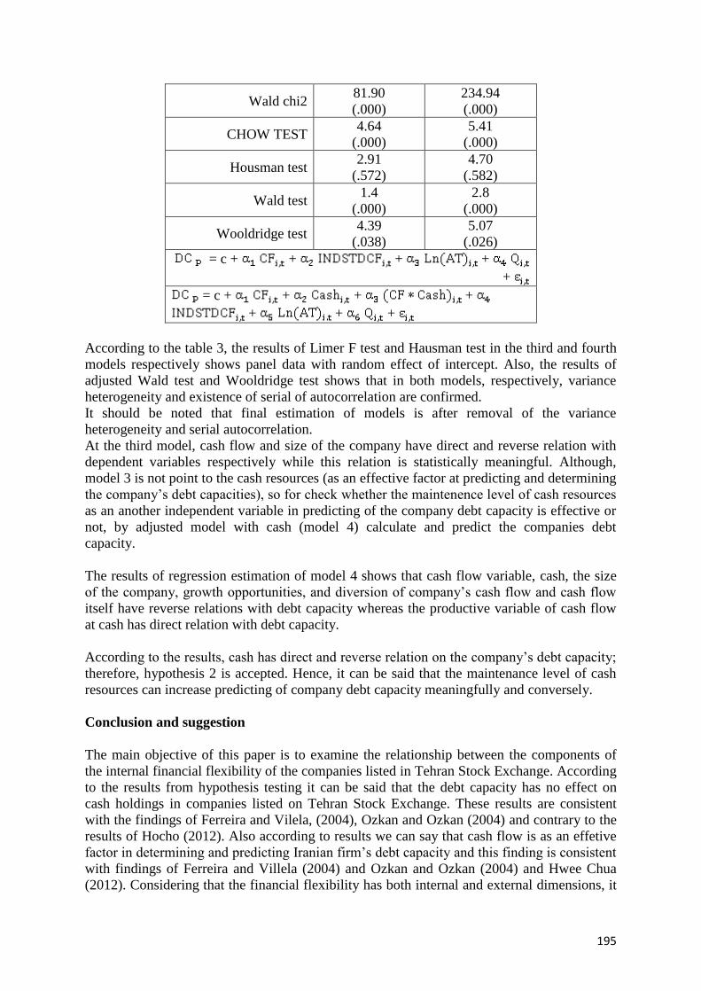
195

Wald chi2 81.90

(.000)

234.94

(.000)

CHOW TEST 4.64

(.000)

5.41

(.000)

Housman test 2.91

(.572)

4.70

(.582)

Wald test 1.4

(.000)

2.8

(.000)

Wooldridge test 4.39

(.038)

5.07

(.026)

= c + + + +

+

= c + + + +

+ + +

According to the table 3, the results of Limer F test and Hausman test in the third and fourth

models respectively shows panel data with random effect of intercept. Also, the results of

adjusted Wald test and Wooldridge test shows that in both models, respectively, variance

heterogeneity and existence of serial of autocorrelation are confirmed.

It should be noted that final estimation of models is after removal of the variance

heterogeneity and serial autocorrelation.

At the third model, cash flow and size of the company have direct and reverse relation with

dependent variables respectively while this relation is statistically meaningful. Although,

model 3 is not point to the cash resources (as an effective factor at predicting and determining

the company’s debt capacities), so for check whether the maintenence level of cash resources

as an another independent variable in predicting of the company debt capacity is effective or

not, by adjusted model with cash (model 4) calculate and predict the companies debt

capacity.

The results of regression estimation of model 4 shows that cash flow variable, cash, the size

of the company, growth opportunities, and diversion of company’s cash flow and cash flow

itself have reverse relations with debt capacity whereas the productive variable of cash flow

at cash has direct relation with debt capacity.

According to the results, cash has direct and reverse relation on the company’s debt capacity;

therefore, hypothesis 2 is accepted. Hence, it can be said that the maintenance level of cash

resources can increase predicting of company debt capacity meaningfully and conversely.

Conclusion and suggestion

The main objective of this paper is to examine the relationship between the components of

the internal financial flexibility of the companies listed in Tehran Stock Exchange. According

to the results from hypothesis testing it can be said that the debt capacity has no effect on

cash holdings in companies listed on Tehran Stock Exchange. These results are consistent

with the findings of Ferreira and Vilela, (2004), Ozkan and Ozkan (2004) and contrary to the

results of Hocho (2012). Also according to results we can say that cash flow is as an effetive

factor in determining and predicting Iranian firm’s debt capacity and this finding is consistent

with findings of Ferreira and Villela (2004) and Ozkan and Ozkan (2004) and Hwee Chua

(2012). Considering that the financial flexibility has both internal and external dimensions, it

196

is recommended that a research should be done on components of foreign financial flexibility

companies listed on Tehran Stock Exchange. It can be suggested to financial managers that in

order to have dynamic and appropriate internal financial flexibility, they should pay special

attention to firm’s cash holding. Because cash resources, in addition to being one of the major

causes of internal financial flexibility, play an important role in determining debt capacity as

another factor in creating internal financial flexibility. Hence it can be concluded that cash

resources play a very important role in forecasting the company's financial flexibility. So

managers will be able to desirably manage crises and make efficient use of unexpected

investment opportunities and increase the firm’s value with continuous attention to cash flow

holding as an effective factor in the management of financial flexibility.

References

1. Almeida, H. Campello, M. & Weisbach, M. S. (2004). 'The Cash Flow Sensitivity of Cash'.

The Journal of Finance, 59(4): 1777-1804.

2. Bates, T. Kahle, K. & Stulz, R. (2009). 'Why Do U.S. Firms Hold so Much More Cash than

They Used to?'. The Journal of Finance, 64(5): 1985-2021.

3. Berger, P. G. Ofek, E. & Swary, I. (1996). 'Investor Valuation of the Abandonment Option'.

Journal of Financial Economics, 42(2): 257-287.

4. Campello, M. Giambona, E. Graham, J. R. & Harvey, C. R. (2011). 'Liquidity Management

and Corporate Investment during a Financial Crisis'. The Review of Financial Studies, 24(6):

1944-1979.

5. Fakhari, H & Taghavi, R. (2009). Quality of Accrual items and Cash. Iranian accounting &

auditing review, 16(57): 69-84.

6. Ferreira. M, and A. Vilela, (2004). “Why do firms hold cash? Evidence from EMU

Countries”, European Financial Management, 10(2): 295–319.

7. Foley, C. F. Hartzell, J. C. Titman, S. & Twite, G. (2007). 'Why do firms hold so much cash?

A tax-based explanation'. Journal of Financial Economics, 86(3): 579-607.

8. Gord, A. Mohammadi, M. & Goldoost, M. (2009). Investigating the relationship between

corporate governance mechanism and cash holding. Iranian accounting & auditing review,

22(2): 263-278.

9. Hwee Chua, Sh. (2012). ‘Cash holdings, Capital structure and financial flexibility’ Thesis

submitted to the University of Nottingham.

197

10. Lins, K. V. Servaes, H. & Tufano, P. (2010). 'What drives corporate liquidity? An

international survey of cash holdings and lines of credit'. Journal of Financial Economics,

98(1): 160-176.

11. Ozkan, A & Ozkan, N. (2004). Corporate cash holdings: An empirical investigation of UK

companies. Journal of Banking & Finance, 28(9): 2103-2134.

12. Saeidi, A & Abesht, K. (2013). Debt capacity in the Firms listed in Tehran Stock Exchange.

Iranian accounting & auditing review, (72): 43-64.

13. Sepasi, S & Yablouyi, M. (2007). Asymmetric Cash Flow Sensitivity of Cash Holdings.

Iranian accounting & auditing revie, 20(4): 61-76.

14. Subramaniam, V. Tang, T. T. Yue, H &. Zhou, X. (2011). ‘Firm structure and corporate cash

holdings’ Journal of Corporate Finance, (17): 759–773.

15. Sufi, A. (2009). 'Bank Lines of Credit in Corporate Finance: An Empirical Analysis'. Review

of Financial Studies, Vol. 22(3): 1057-1088.

16. Volberda, H. W. (1998). ‘Building the Flexible Firm: How to remain Competitive’. Oxford,

Oxford University Press, 2(1): 94-96.

198

THE RELATIONSHIP BETWEEN FOREIGN DIRECT INVESTMENT,

ECONOMIC GROWTH AND UNEMPLOYMENT IN TURKEY: AN EMPIRICAL

ANALYSIS FOR THE PERIOD OF 2008-2015

Faruk Demirhan

Presidency of Tax Inspection Board, Turkey


Mustafa Göktuğ Kaya

Presidency of Tax Inspection Board, Turkey


Perihan Hazel Kaya

Selçuk University, Turkey


Foreign direct investment has an important role for many developing countries. Because

foreign direct investment inwards may provide a positive contribution to economic growth,

employment and technology. So foreign direct investment is extremely important for Turkey

economy. Nevertheless, global financial crisis has affected the foreign direct investment

negatively both in Turkey and in the world. In this study, the effect of foreign direct

investment on the economic growth and unemployment after the global financial crisis in

Turkey has been analyzed. The analysis used quarterly data from the period 2008-2015, the

ADF unit root test, the PP unit root test, impulse-response analysis, variance decomposition

and Granger causality tests, has been applied. As a result, in parallel similar studies in the

literature, it has been observed that foreign direct investment has a positive impact on

economic growth and unemployment. The other words, the increase in foreign direct

investment not only trigger economic growth but also decrease unemployment by creating

employment.

Key Words: Foreign Direct Investment, Economic Growth, Unemployment, Turkey, VAR

Analysis

*This study was derived from the postgraduate thesis titled “The Relationship Between

Foreign Direct İnvestments and Growth: An Empirical Analysis for Turkey After Global

Financial Crisis ”

INTRODUCTION

After industrial revolution, the significance degree in production factors economically

changed. The importance of capital and labor factors come into prominence much more.

Capital has begun to go toward the regions it will make more profit and countries have begun

to attract capital to their own countries. This cycle has become more fast and flexible at the

present days with also the effect of globalization. In commercial meaning, the world, whose

borders are removed, has been begun to be seen as a single country for capital owners.

Capital owners, as in the past, also plan their international investments according to the

economic and political stability, cheap labor force, cheap raw material.

http://tureng.com/tr/turkce-ingilizce/presidency%20of%20tax%20inspection%20board

http://tureng.com/tr/turkce-ingilizce/presidency%20of%20tax%20inspection%20board

199

Direct foreign capital entering country, also with the effects of privatizations made in 2007,

reached the peak point. However, just as 2008 global crisis affected all the world, negatively

affected Turkish economy as well. Turkey postponed global capital investment plans and,

following economic developments, altered its investments according to the new conditions.

Foreign investments, which show an increase compared to the previous years before crisis,

are still continuing their unstable process after crisis in global economy.

The aim of the study, is to investigate the effect of foreign direct investments in Turkey on

economic growth and employment in the period after 2008 Global Crisis. In this direction,

firstly, the process of foreign direct investments in Turkish economy was historically

discussed. Then, it was investigated at what extent 2008 global crisis affects the foreign

direct capital investments inflow the country, and effect of these investments on economic

growth and employment was tested by means of VAR analysis.

1. Foreign Direct Investments and Turkish Economy

Foreign direct investments is that multinational companies (MNCs) and investors make long

term investments in the political borders of another country out of their own countries. This

sort of investments occur in the way of acquiring an existent company, taking in partnership,

or making new investments. According to IMF, foreign direct investment is cross-country

investments, which multinational companies make out of the countries, where their

headquarters are located, in order to stay long time in the different economies

(IMF,1993a:83).According to Kumral (2001:6), foreign direct investment is the investments,

which are carried out by means of global companies being in active in at least two countries,

including home country.

In this direction, investments in the way of that cross-country companies making trade and

investment in global scale attempt the new investments in countries different from countries,

in which their headquarters are located; and that they take in partnership in the existent local

companies, are defined as foreign direct investments. The country making investment is

called “parent company”; the companies in the invested countries, “subsidiary company”;

“foreign company”, or “branch” (Seyidoğlu, 1998:711).

Together with the foundation of Republic, after İzmir Economic Congress in 1923, in the

framework of liberal approach, it was observed that foreign direct investment was made on

the certain areas. But, these investments were actualized via establishing local partnership. In

the early years of Republic, while the number of companies with foreign capital was 94,

when reached 1929, the number of companies with foreign capital rose to 114 and $ 30

million of capital entered the country. After Second World War ended, several legal

arrangements were conducted so that foreign direct investment could enter the country. With

the decision made, dated April 22, 1947, and numbered 13, based on the Law on Protection

of Value of Turkish Currency, “it was foreseen that foreign capital was brought as foreign

currency and invested on the areas such as agriculture, industry, transportation, and tourism.

Provided that the government found the investment of foreign capital useful for development

of the country and in quality increasing export, it can transfer some part of profit that forms

abroad” (Koçtürk and Eker, 2012 :39).

In the framework of import substitution industrialization plan, thanks to these incentives the

government presents to the certain holdings , these holdings began to have voice as much as

involved in industrial policies. These holdings began to draw the companies, which will

undertake a common enterprise with them, to the country with the support of government, not

200

multinational companies (MNCs) that will compete with them. Large states, with the

partnerships they establish with MNCs, did not left living areas for SMSEs much more.

When reached 1980s, Turkish economy experienced a transition period from conservative

economic policy to free economy. This actualized after the package of economic decisions of

January 24, 1980 and Turkey passed to outward- oriented liberal economy. After January 24

decisions, in 1981, foreign investor coming to the country increased.

With the enactment, numbered 32, issued on August 11, 1989, based on the law on Protection

of Value of Turkish Currency, quantity restrictions on foreign capital were removed and it

was allowed for the foreigners to be able to make purchase in capital market in Turkey. This

state caused the increase in foreign direct investments. Beside this, with coming of enactment

into force, in Turkey, the rise of real interest rates resulted in important increases in the

investments foreign direct capital (Göz, 2009 : 87).

High inflation, economic instabilities, amount of increasing domestic and foreign debts, and

high public deficits pushed Turkish economy into 1994-1999-2001 crisis. Any of economic

reforms made between the years of 1980-2001 could not prevent these crises. The causes

such as high real interests and insufficient domestic savings led increasing effects of

economic crises. The reforms made for foreign investors and tax incentives did not become

effective in crisis environment (Şener and Kılıç ,2008 : 22-49).

In Turkey, for the encouraging FDIs, Agreement of Mutual Protaction and Encouragement of

Investments was signed with 85 countries. With 76 countries, agreement on prevention of

double taxation was signed and with 19 countries, Free Trade Agreement (Müsiad, 2014 68).

As a result of the law issued in 2002 and economic and political stability, inflow of foreign

direct investment has increased every years and reached the peak point in 2007. After 2002,

increase of privatizations functions as an instrument for foreign capital to enter Turkey

(Bayraktar, 2003:47).Some of large scale privatizations and acquirements of company are the

sales of Türk Telekom, Turkcell, Garanti and Fortis Bank.

Financial crisis beginning in US economy, created by housing credits, spread all economies

of the world in the short time and this crisis would also negatively affect international

investments, since it will result in recession. One of the most affected from the crisis is also

Turkey. With the effect of privatizations, acquirements of companies, and mergers, between

2004-2007, high amount of foreign direct investment was taken in the country and economic

growth was realized. A point to be paid attention here is that foreign direct investors entering

Turkey realize company acquirements and mergers instead of making new investments.

These companies acquired companies via privatizations and made on investments on real

estates. Due to the increase of costs and risks after crisis, inflow of foreign direct capital will

decrease and this will negatively affect the growth (Alagöz et al, 2008: 79).

201

Graph 1: International Foreign Direct Investments in Turkey in the Period of 1996-

2014 (Million Dollar)

Source: Central Bank of Turkey Republic, www.tcmb.gov.tr

As will be seen from Graph 1, foreign direct capital investments entering Turkey showed

increase. One of the reasons for total investments not to reach 2007 level is that privatization

is more during 2007 and before.

Mortgage crisis experienced in USA pushed international capital into the markets, where it

can make more profit. However, after 2008 Crisis, foreign capital investments made in the

world did not follow a stable course. The data of economic growth in the world economy

prompted investors to behave more prudent.

Table 1: Developments in The Economic Growth of Turkey in the Period of 2002-2015

Years

GDP

(Billion

USD)

Per Capital

Income

(USD)

Growth

(%) Inflation(%)

Unemployment

(%)

Fiscal

Deficit

(%)

Current

Deficit

(%)

2002 231 3.492 6,2 29,8 10,8 -11,2 -0,3

2003 305 4.565 5,3 18,4 11 -8,8 -2,5

2004 390 5.775 9,4 9,3 10,8 -5,4 -3,7

2005 482 7.036 8,4 7,7 10,6 -1,5 -4,6

2006 526 7.597 6,9 9,6 10,2 -0,5 -6,1

2007 649 9.247 4,7 8,4 10,3 -1,6 -5,9

2008 742 10.444 0,7 10,1 11 -1,8 -5,7

2009 617 8.561 -4,8 6,8 14 -5,5 -2,2

2010 732 10.079 9,2 6,4 11,9 -3,6 -6,2

2011 774 10.444 8,8 10,5 9,8 -1,3 -9,7

2012 786 10.497 2,2 6,2 9,2 -2,2 -6,1

2013 823 10.822 4,2 7,4 9,7 -1,2 -7,9

2014 800 10.404 2,9 8,2 10,9 -1,3 -5,4

2015 718 9.261 4 8,8 10,3 -1,2 -4,5

Source: Central Bank of Turkey Republic, www.tcmb.gov.tr; World Bank Database,

www. worldbank.org

http://www.tcmb.gov.tr/

202

Economic growth has fallen after 2011.The reason for this case is the internal dynamics of

the country, and the effect of slowing in world economy has a major share. As will also be

seen from the data of world investment report, total world investments show a decrease. This

state mostly affects the developing countries economies.

2. Literature

In the literature, while the studies dealing with the relationship of foreign direct investments

and economic growth are quite more, the studies dealing with the relationship of foreign

direct investments, economic growth, and unemployment are very restricted.

Balasubramanayam et al.(1996), as a result of the studies they carried out on 18 developing

countries, which follow export -oriented development policy, identified that foreign direct

capital investments had a positive effect on economic development and, in addition, with

liberalization of foreign trade, that there was a linearity relationship between foreign direct

investments and economic development.

DeMello (1999), in his study, which is related to the period of 1970–1999, on OECD member

and non- OECD member country, observed that according to the production increase,

increase in total factor productivity, increase in capital accumulation, and level of

technological deficit, the relationship of foreign direct investment and growth varied. In this

direction, as technological deficit increases, the effect of foreign direct investments on the

growth falls.

Alfaro et al.(2001) studied the effect of presence of domestic financial market and foreign

direct investments on economic growth. As a result of this study including the period of

1975-1995, they identified that the presence of domestic financial market and foreign direct

investments are the effective instruments in increasing economic growth.

Mencinger (2003) studied the range of 1994-2000 of the countries passing to market

economy. He did not find any cause – result relationship between FDI/GDP and fixed capital

investments/GDP. He attributed the cause of this to rapidly performed privatization and

company acquirements.

Lyroudı et al. (2004), in the study they carried out, observed that, as a result of econometric

analysis they carried out on economic growths of transition economies, foreign direct

investments did not have an important effect on the growth of transition economies.

Demirel (2006) studied how foreign direct capital affected GDP of Turkey. In his study, he,

using the least squares technique with three stages, which include growth equations, made

economic modeling and, reached the conclusion that GDP of Turkey was positively and

significantly affected from in foreign direct investment inflows.

Khaliq and Noy (2007) studied the sectorial effect of foreign direct investments in Indonesia

and, at the end of the studies, observed that foreign direct investments positively affected the

economic growth but in respect with the sectors, showed change.

Ekinci (2011), in his study, using the data of the period of 1980-2010, studied the relationship

between foreign direct investments, economic growth and employment. According to the

results of causality analysis, while a long term relationship was found between foreign direct

investments and economic growth, between foreign direct investments and employment, any

relationship could not be identified.

203

Özcan (2014), in his study, studied the periods of 1980-2003 and 2003-2012 by means of

Augmented Dickey Fuller test, Johansen Co-integration Analysis, Vector Error Correction

and Granger Causality Analysis and reached the conclusion that foreign direct capital

investments in Turkey were not the cause of growth.

3. Empirical Analysis

In this section, on the purpose of seeing the effects of foreign direct capital on economy in

the period after global financial crisis, by means of econometric tests, applied analysis has

been carried out.

3.1. Methodology

The universe of our study consists of foreign direct investments entering Turkey and our

sample includes the figures of economic growth and unemployment in the range of years of

2008 and 2015.

3.1.1. VAR Model

VAR Model, among time series model, is the most used one in the recent times. Sims (1980),

Dijk and Franses (2000), Johansen (2000), Kilian and Chang (2000), and Lutkepohl (2000)

can be shown as example for the literature in the recent literature about VAR modeling and

analysis (Özgen and Güloğlu, 2004: 4).

VAR, revealing the mutual relationships between the variables, is used for shaping

macroeconomic policies. Vector time series models are the ones, in which more than one

variables take place, but which include all features of univariate models. In other words,

stationarity and prediction conditions that are necessary for univariate stochastic processes

and the case that model is reversible, and its roots are out of unit circle are also valid for

vector processes. VAR approach has become a method adopted by econometrists in the

recent times.

Bivariate VAR Model can be expressed in standard way as follows:

1 1 2 11 1

p p

i i t i tt t ii i

y ya b b x v

1 1 2 21 1

p p

t i i t i tt ii i

yx c d d x v

In the above model, ρ represents the length of lags; v, randomized error terms, whose mean

value is zero; whose variances with their own lagged values are zero and fixed; and which

has normal distribution. The assumption that in VAR Model, the errors are irrelevant with

their own lagged values does not bring any constraint on the model. For, with increasing the

lagging length of the variables, the problem with autocorrelation is coped with (Özgen and

Güloğlu, 2004: 96).

Pagan (1987) summarizes VAR model in four steps:

204

• The data are converted into a suitable form to VAR.

• By means of causality test, lagging values and variables are selected.

• Reducing lagging value and smoothing coefficients, VAR is tried to be made

simpler.

• Shocks are obtained by the process of orthogonalization.

3.2. Model and Hypothesis

In this model formed to examine the effects of foreign capital investments on economy, as

representative of long term capital entering the country, in accordance with the literature, the

variable “foreign direct capital” is used. In order to measure the effects of foreign capital

investments on economy, economic growth was used. Hence, the variable “gross domestic

product” was added to the model. In addition, on the name of seeing the effects of foreign

direct investment on the economy, the data of employment were added to the model. In this

context, just as the number of person employed in the economy can be used, the number of

persons, who is ready to be employed but cannot be employed in economy, can also be used.

In this context, the number of unemployed people was also added to the model.

In this direction, in the model, the variables of amount of foreign direct capital, gross

domestic product with fixed prices, and the number of unemployed people were used. The

hypotheses established to each other of these variables are as follows:

Hypothesis 1: The increase in the amounts of foreign direct capital entering economy leads

economic magnitudes to increase.

In an economy, increase of investments will increase both investments and amount of product

that will be produced as a result of investments and this will cause economic magnitudes to

show an increase.

Hypothesis 2: The increase in foreign direct capital investments entering economy leads

unemployment to decrease.

Increase of investments in an economy, besides the increase of amount of production,

depending on whether the investment to be made is labor intensive or capital intensive, will

lead labor input in the production process to be more used.

Hypothesis 3: The increase in economic magnitude will cause unemployment to decrease.

The increase in economic magnitude means that the production and investments in the

economy increase. Especially the increase in the production process means that the need for

labor input increases, which also means that the number of unemployed people decreases.

In the light of all hypotheses to be planned to test, the expected result is that an increase in

foreign direct investments helps economy grow and that there is a decrease in the number of

unemployed people.

3.3.Data Definitions

The data belonging to the variables to be used in the analyses, differently from the existing

literature, after the global financial crisis emerging the last months of 2007, in order to

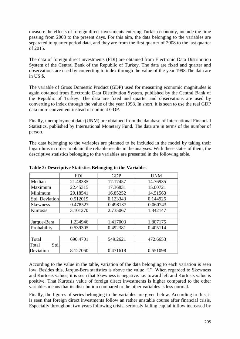
205

measure the effects of foreign direct investments entering Turkish economy, include the time

passing from 2008 to the present days. For this aim, the data belonging to the variables are

separated to quarter period data, and they are from the first quarter of 2008 to the last quarter

of 2015.

The data of foreign direct investments (FDI) are obtained from Electronic Data Distribution

System of the Central Bank of the Republic of Turkey. The data are fixed and quarter and

observations are used by converting to index through the value of the year 1998.The data are

in US $.

The variable of Gross Domestic Product (GDP) used for measuring economic magnitudes is

again obtained from Electronic Data Distribution System, published by the Central Bank of

the Republic of Turkey. The data are fixed and quarter and observations are used by

converting to index through the value of the year 1998. In short, it is seen to use the real GDP

data more convenient instead of nominal GDP.

Finally, unemployment data (UNM) are obtained from the database of International Financial

Statistics, published by International Monetary Fund. The data are in terms of the number of

person.

The data belonging to the variables are planned to be included in the model by taking their

logarithms in order to obtain the reliable results in the analyses. With these states of them, the

descriptive statistics belonging to the variables are presented in the following table.

Table 2: Descriptive Statistics Belonging to the Variables

FDI GDP UNM

Median 21.48335 17.17457 14.76935

Maximum 22.45315 17.36831 15.00721

Minimum 20.18541 16.85252 14.51563

Std. Deviation 0.512019 0.123343 0.144925

Skewness -0.478527 -0.498137 -0.060743

Kurtosis 3.101270 2.735067 1.842147

Jarque-Bera 1.234946 1.417003 1.807175

Probability 0.539305 0.492381 0.405114

Total 690.4701 549.2621 472.6653

Total Std.

Deviation 8.127060 0.471618 0.651098

According to the value in the table, variation of the data belonging to each variation is seen

low. Besides this, Jarque-Bera statistics is above the value “1”. When regarded to Skewness

and Kurtosis values, it is seen that Skewness is negative. i.e. toward left and Kurtosis value is

positive. That Kurtosis value of foreign direct investments is higher compared to the other

variables means that its distribution compared to the other variables is less normal.

Finally, the figures of series belonging to the variables are given below. According to this, it

is seen that foreign direct investments follow an rather unstable course after financial crisis.

Especially throughout two years following crisis, seriously falling capital inflow increased by

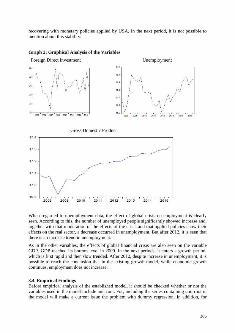
206

recovering with monetary policies applied by USA. In the next period, it is not possible to

mention about this stability.

Graph 2: Graphical Analysis of the Variables

Foreign Direct Investment Unemployment

Gross Domestic Product

When regarded to unemployment data, the effect of global crisis on employment is clearly

seen. According to this, the number of unemployed people significantly showed increase and,

together with that moderation of the effects of the crisis and that applied policies show their

effects on the real sector, a decrease occurred in unemployment. But after 2012, it is seen that

there is an increase trend in unemployment.

As in the other variables, the effects of global financial crisis are also seen on the variable

GDP. GDP reached its bottom level in 2009. In the next periods, it enters a growth period,

which is first rapid and then slow trended. After 2012, despite increase in unemployment, it is

possible to reach the conclusion that in the existing growth model, while economic growth

continues, employment does not increase.

3.4. Empirical Findings

Before empirical analysis of the established model, it should be checked whether or not the

variables used in the model include unit root. For, including the series containing unit root in

the model will make a current issue the problem with dummy regression. In addition, for

207

being able to identify the relationships between the variables to be used in Vector Auto

Regression (VAR), it is necessary for the variables to be stationary. Therefore, it is necessary

to test whether or not there is a test problem with the variables. Before establishing VAR

model whether or not the variables are stationary is identified by linear unit root test, which

are developed by Dickey-Fuller (1979,1981, ADF) and Phillips-Perron (1988, PP).

Table 3: Results of Stationarity Test

ADF PP

Level Variables

Constant

FDI

-3.543

[0.0133]**

-3.543

[0.0133]**

GDP

0.3904

[0.979]

-1.581

[0.480]

UNM

-3.527

[0.014]**

-1.941

[0.309]

Constant+Trend

FDI

-3.509

[0.055]*

-3.441

[0.064]*

GDP

-3.5972

[0.047]*

-5.121

[0.001]***

UNM

-3.506

[0.058]*

-1.848

[0.656]

First Difference

Constant

FDI

-7.856

[0.000]***

-8.121

[0.000]***

GDP

-4.200

[0.000]***

-6.706

[0.000]***

UNM

-3.186

[0.032]**

-5.913

[0.000]***

Constant+Trend

FDI

-7.798

[0.000]***

-8.107

[0.000]***

GDP

-17.743

[0.000]***

-6.475

[0.000]***

UNM

-4.099

[0.017]**

-5.809

[0.000]***

Note: *, ** and *** are represented respectively %10, %5 ve %1 the

values of significance level. The values in parentheses are the values of

probability. For ADF unit root test, %1, %5, ve %10 confidence interval,

Mac Kinnon (1996) critical values are -3.485. -2.885. -2.579 for constant

model; -4.035. -3.447. -3.148 for constant and trend model. For PP test,

%1, %5 ve %10 confidence interval, Mac Kinnon (1996) critical values

are -3.483. -2.884. -2.579 for constant model; -4.033. -3.446 ve 3.148 for

constant and trend model.

For the stationarity of the variables, it is necessary for the estimated τ (tau) statistical value of

the variable to be bigger in terms of absolute value than table value ( h t ), developed by

MacKinnon (1996). In other word, with a simpler method, it is necessary for the probability

values given in bracket to be smaller than significance level (1-0.01%, 5-0.05% and 10-

208

0.1%). When regarded to the level values of series, it is seen that they generally have unit

root. According to the result of both tests, series of foreign direct investments is stationary at

the level in the confidence interval of 5% and in in the confidence level of 10% in the model

constant and with constant–trend. However, it is seen that the series, whose first difference is

taken, is stationary at the significance level of 1% in the model constant and with constant–

trend. In view of this, it can be said that that series is included in the model with their first

differences is proper.

When the level values of the series belonging to the variable of gross domestic product is

examined, it is seen that the model with constant has unit root, while in the model with

constant and trend, they are stationary in ADF and PP test results are stationary at the

significance level of 5% and 1%. However, both test results, it is understood that in the first

difference of series at the significance level of 1%, the models with constant, and with

constant and trend are stationary. Assuming that the variable of gross domestic product

shows a feature of long memory, it can be said that in this variable, that analysis is continued

by adding the first differences is proper.

Finally, when the level values of series belonging to the variable unemployment are

examined, it is seen that while ADF test finds stationarity at the significance level of 5% in

the model with constant and 10% in the model with constant and trend, PP test did not find

stationarity in any model. When the first difference of the series is taken, it is seen that PP

test presented evidences regarding that it became stationary at the significance level of 1%.

However, the results of ADF test reports that unemployment series became stationary in its

first difference in the model with constant and trend at the significance level of 5%. In this

case, as in GDP series, in the framework of the assumption that it showed the feature of long

memory, it will be proper to include the first difference of series in the model.

After unit root analysis, using the first difference of series, VAR Model is formed. While

conventional VAR analyses are established, in the first stage, the first test that is necessary to

be made is to determine the proper lagging time. For this aim, the test of lagging number is

made and two lags are identified according to Schwarz information criterion. However, with

auto correlation test, the presence of auto correlation is identified. In two lagged model, since

it is seen that there is a problem with auto correlation, until this problem is removed, lagging

number is increased. In five lagged model, it was seen that the problem with auto correlation

was eliminated. Therefore, there are five lags in the analysis.

In the second stage, action-reaction analysis is carried out. In Table 4, the reactions each

variable gave to the positive shocks in the other variables are summarized. According to this,

the reaction the variable GDP gave to a positive shock occurring within itself are very

positive and it is significant throughout the period. This case is significant both statistically

and economically. The reaction GDP gave to 1% increase occurring in foreign direct

investments is positive. The result maintains statistical significance throughout four periods.

On the other hand, the result seems to be significant statistically, For, it is stated in

Hypothesis 1 that increase in foreign direct investments will positively affect economy. The

reaction the economic growth gave to the positive shock in unemployment is negative. The

reaction is negative throughout the period experienced is negative and is statistically

significant. When examined in the framework of economic theory, the result is economically

significant, because a falls in employment will negatively affect the economic magnitudes

due to decrease in the production.

209

Table 4: The Reaction Of GDP

GDP FDI UNM

1 0.017596 0.000588 -0.004924

(0.00244) (0.00345) (0.00338)

2 0.021747 0.005232 -0.013820

(0.00617) (0.00645) (0.00690)

3 0.012621 0.008058 -0.014899

(0.00864) (0.00810) (0.00953)

4 0.010227 0.002292 -0.007219

(0.00818) (0.00827) (0.01082)

5 0.017804 -0.005483 -0.003507

(0.00715) (0.00830) (0.01134)

6 0.017198 -0.005760 -0.010091

(0.00818) (0.00835) (0.01211)

7 0.007300 0.003693 -0.016494

(0.00913) (0.00840) (0.01346)

8 0.006745 0.003889 -0.011239

(0.00838) (0.00825) (0.01341)

9 0.012859 -1.19E-05 -0.005854

(0.00713) (0.00787) (0.01273)

10 0.014665 0.000419 -0.010792

(0.00624) (0.00774) (0.01242)

The reaction the variable foreign direct investment will give to 1% positive shock that will be

experienced in the other variables is summarized in the following table. According to this, the

reaction it will give to the shock in foreign direct investments is positively and statistically

significant. The reaction continues in this way throughout the period. The effect of 1%

increase on foreign direct investments is negative and its statistical significance continues

throughout four quarter. This may be a case related to the composition of foreign direct

investments in Turkey, because it is possible for the investments having labor intensive

production structure to be affected from the developments in the employment. The reaction

of the variable foreign direct investment to 1% positive shock in the variable Gross Domestic

Product is negative and it only continues throughout one period. This case reduces the

statistical significance of the reaction. When economically regarded to, this shows that the

growth of economy has a negative effect on foreign direct investments.

210

Table 5: The Reaction of FDI

GDP FDI UNM

1 -0.014841 0.443991 -0.175469

(0.08705) (0.06157) (0.08360)

2 0.232868 0.188996 -0.020629

(0.14138) (0.13101) (0.15381)

3 0.146719 0.279898 -0.015740

(0.16977) (0.15738) (0.18489)

4 0.308101 0.094217 -0.064516

(0.15843) (0.16720) (0.20663)

5 0.207400 0.043563 0.032586

(0.15876) (0.17904) (0.22196)

6 0.223855 0.171390 -0.173499

(0.15275) (0.17320) (0.22199)

7 0.254375 0.054330 -0.036498

(0.14773) (0.17386) (0.23313)

8 0.103205 0.276271 -0.206783

(0.15128) (0.16364) (0.22893)

9 0.212631 0.061405 -0.013655

(0.14742) (0.17750) (0.23414)

10 0.096669 0.174921 -0.090453

(0.14271) (0.17796) (0.22629)

The reaction the variable unemployment gave to the positive shocks experienced in gross

domestic product and foreign direct investments is shown in the following table. According

to this, the reaction it gave to a shock occurring the variable unemployment is positive and it

is statistically and economically significant. The variable unemployment gives a negative

reaction to a positive development occurring in gross domestic product. The result is negative

and statistically significant throughout all period. İt is also economically significant. For, the

growth of economy brings together the decrease of unemployment with it. The reaction the

variable unemployment gave to foreign direct investments is negative. When the result is

economically evaluated, it is possible to say that foreign direct investments enter economy in

such a way that forms employment.

211

Table 6: The Reaction of UNM

GDP FDI UNM

1 -0.017713 -0.025015 0.063296

(0.01217) (0.01192) (0.00878)

2 -0.044185 -0.038012 0.082611

(0.02420) (0.02304) (0.02336)

3 -0.040482 -0.039364 0.095318

(0.03465) (0.03248) (0.03595)

4 -0.043805 -0.034740 0.084525

(0.03888) (0.03722) (0.04685)

5 -0.046761 -0.037023 0.104243

(0.04132) (0.04139) (0.05424)

6 -0.044750 -0.031407 0.095954

(0.04433) (0.04122) (0.06156)

7 -0.031949 -0.035492 0.109287

(0.04702) (0.04234) (0.06875)

8 -0.036930 -0.031870 0.095693

(0.04605) (0.04217) (0.07373)

9 -0.035669 -0.037981 0.109966

(0.04644) (0.04322) (0.07725)

10 -0.036210 -0.039849 0.102198

(0.04427) (0.04276) (0.07948)

After action - reaction analysis, the results of variance decomposition analysis testing that a

shock occurring in each variable can be explained by variance analysis are given in the

following table. According to the results of variance decomposition analysis, in the first

period, all of a shock experienced in GDP is explained by GDP. In the progressing quarters,

the ability of both unemployment and foreign direct investments to account for economic

growth has increased. In the 10th quarter, 20% of shock in GDP is explained by foreign direct

investments and 25%, by the variable unemployment. This result shows that foreign direct

investments have an important place in Turkish economy.

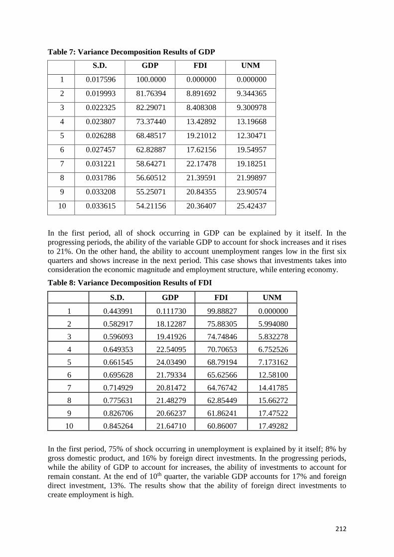
212

Table 7: Variance Decomposition Results of GDP

S.D. GDP FDI UNM

1 0.017596 100.0000 0.000000 0.000000

2 0.019993 81.76394 8.891692 9.344365

3 0.022325 82.29071 8.408308 9.300978

4 0.023807 73.37440 13.42892 13.19668

5 0.026288 68.48517 19.21012 12.30471

6 0.027457 62.82887 17.62156 19.54957

7 0.031221 58.64271 22.17478 19.18251

8 0.031786 56.60512 21.39591 21.99897

9 0.033208 55.25071 20.84355 23.90574

10 0.033615 54.21156 20.36407 25.42437

In the first period, all of shock occurring in GDP can be explained by it itself. In the

progressing periods, the ability of the variable GDP to account for shock increases and it rises

to 21%. On the other hand, the ability to account unemployment ranges low in the first six

quarters and shows increase in the next period. This case shows that investments takes into

consideration the economic magnitude and employment structure, while entering economy.

Table 8: Variance Decomposition Results of FDI

S.D. GDP FDI UNM

1 0.443991 0.111730 99.88827 0.000000

2 0.582917 18.12287 75.88305 5.994080

3 0.596093 19.41926 74.74846 5.832278

4 0.649353 22.54095 70.70653 6.752526

5 0.661545 24.03490 68.79194 7.173162

6 0.695628 21.79334 65.62566 12.58100

7 0.714929 20.81472 64.76742 14.41785

8 0.775631 21.48279 62.85449 15.66272

9 0.826706 20.66237 61.86241 17.47522

10 0.845264 21.64710 60.86007 17.49282

In the first period, 75% of shock occurring in unemployment is explained by it itself; 8% by

gross domestic product, and 16% by foreign direct investments. In the progressing periods,

while the ability of GDP to account for increases, the ability of investments to account for

remain constant. At the end of 10th quarter, the variable GDP accounts for 17% and foreign

direct investment, 13%. The results show that the ability of foreign direct investments to

create employment is high.

213

Table 9: Variance Decomposition Results of UNM

S.D. GDP FDI UNM

1 0.063296 7.831600 16.38545 75.78295

2 0.070372 20.48582 17.15178 62.36240

3 0.072103 19.77727 16.36687 63.85586

4 0.073209 19.39050 16.25689 64.35261

5 0.076144 18.07491 15.12556 66.79952

6 0.076636 17.91233 15.48242 66.60525

7 0.079779 19.10322 14.49711 66.39967

8 0.081517 18.67054 14.06539 67.26407

9 0.082939 18.05906 14.12342 67.81752

10 0.083560 17.79596 13.96536 68.23868

Finally, in order to examine causality relationship between variables, VAR based Granger

causality analysis is carried out. The results of causality analysis, contrast to the results

obtained from action-reaction and variance decomposition analysis, presents evidences

regarding that there is no causality relationship between variables. Causality relationship is

only from the variable GDP to foreign direct investments and its significance level is 5%.

Table 10. Granger Causality Analysis Results

Hypothesis Wald Statistics Probability Value Result

GDP is not the cause

of FDI. 11.16 0.0483

There is a

causality from

GDP to FDI

GDP is not the cause

of UNM. 3.82 0.5749

There is no

causality from

GDP to UNM

FDI is not the cause

of GDP. 4.06 0.5406

There is no

causality from

FDI to GDP

FDI is not the cause

of UNM. 0.85 0.9736

There is no

causality from

FDI to UNM

UNM is not the

cause of GDP. 2.21 0.8188

There is no

causality from

UNM to GDP

UNM is not the

cause of FDI. 2.21 0.1339

There is no

causality from

UNM to FDI

When the results obtained from all analyses are evaluated together, it is possible to say that

foreign direct investments have an important role for Turkish economy in the post crisis

period. the increase in foreign direct investments not only triggers economic growth but also

reduce unemployment, creating employment. In the last period, it will be true to say that the

214

increase of foreign direct investments having an extremely important role in the increase of

gross domestic product will be an important factor of high rate growth in the progressing

years. In addition, as the solution of the problem with unemployment experienced in Turkey,

it is also useful to repeat that utilizing foreign direct investments will be a proper strategy.

CONCLUSION

Just as 2008 global economic crisis affected all countries of the world, it also negatively

affected Turkish economy. That global capitalists avoid risk caused the new investments,

which will be made, to be delayed or cancelled. This case led world economy to shrink.

Globalization of economy causes a negative case occurring in the developed countries to

directly affect the developing market economies.

In the study we have carried out, post crisis development of foreign direct investments and its

effect on Turkish economy were analyzed by establishing an economic model. In the model,

the variables of amount of foreign direct capital, gross domestic product with fixed prices,

and the number of unemployed people were used. First of all, whether or not there is a

problem with unit root in the variables was tested and before establishing a model in this

direction, linear unit root test, which was developed by Dickey-Fuller (1979,1981, ADF) and

Phillips-Perron (1988, PP), and which did not take into consideration the structural

vulnerabilities. According to the result of both tests, the series of foreign direct investments is

stationary in the confidence intervals of 5% in the model with constant at the level and 10%

in the model with constant and with constant–trend.

When the level values of the series belonging to the variable gross domestic product are

examined, it was seen that the model with constant had unit root and, in the model with

constant and trend, ADF and PP test results are stationary at the significance levels of 5% and

1%

When the level values of the variable unemployment are examined, it was seen that while

ADF test finds stationary at the significance level of 5% in the model with constant, PP test

did not find stationary in any model, and when the first difference of series is taken, that the

evidences regarding that PP test became stationary at the significance level of 1%.

In the second stage, in the action-reaction analysis carried out, the reaction the variable GDP

gave to the positive shock occurring within itself is positive and is significant throughout the

period. This case is significant both statistically and economically. It was seen that the

reaction GDP gave to 1% increase occurring in foreign direct investments was positive.

It was observed that while the reaction 1% increase in unemployment gave to the positive

shock was statistically significant, its effect on foreign direct investments was negative and

its statistical significance continued throughout four periods. This can be a case related to the

composition of foreign direct investments coming to Turkey.

The reaction the variable unemployment gave to the shock occurring within itself is positive

and is statistically and economically significant. The variable unemployment gave negative

reaction a positive development in gross domestic product.

In variance decomposition analysis, as a result of variations experienced in GDP, it is

understood that foreign direct investments has an important role in Turkish economy. In the

215

variations experienced in foreign direct capital, it is seen that investments consider the

economic magnitude and employment, while entering economy. In the variations occurring in

unemployment, as a result of the analysis, it was observed that the ability of foreign direct

investments to create employment was high.

Finally, in order to observe causality relationship between variables, Granger causality

analysis was carried out. In the results of causality analysis obtained, in contrast to the results

obtained from action-reaction variance analyses, presented the evidences regarding that there

was no significant causality relationships between variables. Causality relationship is from

only the variable gross domestic product to foreign direct investments and significance level

is only 5%.

When the results obtained from all analyses are evaluated together, it is possible to say that

foreign direct investments have an important role for Turkish economy in the post crisis

period. For, the increase in foreign direct investments not only triggers economic growth but

also reduce unemployment, creating employment. In the last period, it will be true to say that

the increase of foreign direct investments having an extremely important role in the increase

of gross domestic product will be an important factor of high rate growth in the progressing

years. In addition, as the solution of the problem with unemployment experienced in Turkey,

it is also useful to repeat that utilizing foreign direct investments will be a proper strategy.

In this direction, Turkey should continue foreign capital to take in the country; follow what

the other developing and developed countries do about this issue; and update itself in this

meaning. In addition, Turkey should pay attention to financial stability and enable foreign

capital to feel itself in security.

RESOURCE

1. Alagöz, M., Erdoğan, S. ve Topallı, Nurgün (2008); Doğrudan Yabancı Sermaye Yatırımları

Ve Ekonomik Büyüme: Türkiye Deneyimi 1992-2007, Gaziantep Üniversitesi Sosyal

Bilimler Dergisi, 7(1): 79-89.

2. Alfaro, L., C. Areendam , Kalemli-Ozcan, Ş. and Sayek, S., (2001), Fdı And Economic

Growth: The Role Of Financial Markets, Harvard Business School, Working Paper 01-083.

3. Balasubramanyam, Venkataraman N., Salisu Mohammed A. and Sapsford D., (1996),

Foreign Direct Investment And Growth İn Ep And Is Countries, Economic Journal, 106

4. Bayraktar, F. (2003) Dünyada Ve Türkiye’de Doğrudan Yabancı Sermaye Yatırımları,

Türkiye Kalkınma Bankası A.Ş., Genel Araştırmalar, Ga/03-1-1, Ankara.

5. De Mello Jr.,and Luiz R. (1999), Foreign Direct Investment-Led Growth: Evidence From

Time Series And Panel Data, Oxford Economic Papers, 51

6. Demirel ,O. (2006). Doğrudan Yabancı Yatırımlar, Ekonomik Büyümeye Etkileri Ve

Türkiye Uygulaması, Süleyman Demirel Üniversitesi Sosyal Bilimler Enstitüsü İktisat

Anabilim Dalı Yüksek Lisans Tezi. Isparta

216

7. Ekinci A.(2011). Doğrudan Yabancı Yatırımların Ekonomik Büyüme Ve İstihdam Etkisi:

Türkiye Uygulaması 1980-2010, Eskişehir Osmangazi Üniversitesi İİBF Dergisi, V.6/2

8. ENDERS, W., 2004. Applied Econometric Time Series (Second Edition), Danvers:Wiley,

9. EUROSTAT. European Union Foreign Direct Investment Yearbook 2007. 2007.

Luxembourg. http://epp.eurostat.ec.europa.eu. (A.D.:02.11.2015).

10. Göz Devlet. “Doğrudan Yabancı Sermaye Yatırımları Ve Türkiye”. Yayınlanmamış

Yüksek Lisans Tezi. Çukurova Üniversitesi Sbe, 2009.

11. IMF, Balance Of Payments Manual. Usa, 1993, S.83. (a) www.imf.org. (Erisim Tarihi:

16.01.2016).

12. Khaliq A. and I. Noy,(2007), Foreign Direct Investment And Economic Growth: Empirical

Evidence From Sectoral Data ın Indonesia, Working Papers

13. Koçtürk M. ve M. Eker (2012), Dünyada Ve Türkiye'de Doğrudan Yabancı Sermaye

Yatırımları Ve Çok Uluslu Şirketlerin Gelişimi , Tarım Ekonomisi Dergisi, Cilt.1, Sayı.18

14. Kumral Neşe (2001), Doğrudan Dış Yatırımlar Ve Bölgesel Kalkınma: Ege Bölgesi

İmalat Sanayi Örneği. Ege Üniversitesi İktisadi Ve İdari Bilimler Fakültesi Yayınları. No:2.

Lyroudı K. , Papanastasıou J. ,Vamvakıdıs A. (2004) Foreign Direct Investment And

Economic Growth In Transition Economies, South Eastern Europe Journal Of Economics

15. Mencinger Jože, (2003), Does Foreign Direct Investment Always Enhance Economic

Growth?, Kyklos, 56

16. MÜSİAD (2014), Doğrudan Yabancı Yatırımların Yerli Şirketler Üzerine Etkileri,

Araştırma Raporları:90

17. OECD (2008), Grim Outlook For Fdı And Shifting Global Investment Patterns, Investment

News, Issue 8, November 2008. www.oecd.org.

18. Özcan M.E. (2014). Doğrudan Yabancı Sermaye Yatırımlarının Türkiye’nin Ekonomik

Büyümesindeki Rolü: 2003 Öncesi Ve Sonrası, Galatasaray Üniversitesi Sosyal Bilimler

Enstitüsü İktisat Anabilim Dalı Yüksek Lisans Tezi. İstanbul

19. Özgen, F. B. ve Güloğlu, B., (2004). Türkiye’de İç Borçlanmanın İktisadi Etkilerinin Var

Tekniği İle Analizi, ODTÜ Gelişme Dergisi, Sayı 31

20. Seyidoğlu, H.(1998) Uluslararası İktisat – Teori, Politika Ve Uygulama. İstanbul.

Geliştirilmiş 12. Baskı. Güzem Yayınları. No. 14.

http://www.imf.org/

http://www.oecd.org/

217

21. Şener S. and Kılıç C. (2008). Osmanlı’dan Günümüze Yabancı Sermaye. Bilgi, 16(1)

22. Tarı R., and Bozkurt H., (2006). Türkiye’de İstikrarsız Büyümenin VAR Analizi (1991.1-

2004.3), İstanbul Üniversitesi Ekonomi ve İstatistik Dergisi, 12(28)

23. TCMB, EVDS, www.tcmb.gov.tr (A.D.:30.10.2015).

24. TUİK, www.tuik.gov.tr (A.D.:20.05.2016).

25. UNCTAD, “World Investment Report 1999 – Foreign Direct Investment And The

Challenge Of Development”. 1999 (b) www.unctad.org. (A.D.:12.12.2015).

26. UNCTAD. “World Investment Report 2006: Fdı From Developing And Transition

Economies: Implications For Development”. New York And Geneva. 2006 (a)

www.unctad.org. (A.D.:12.12.2015).

27. UNCTAD, Assessing The Impact Of The Current Financial And Economic Crisis On Global

Fdı Flows, January 2009(a). www.unctad.org. (A.D.:21.03.2016).

28. UNCTAD, World Investment Report 2009: Transnational Corporations, Agricultural

Production And Development, United Nations, New York, July 2009(b). www.unctad.org.

(A.D.:21.03.2016).

29. UNCTAD World Investment Prospects Survey 2010-2012, 2010, www.unctad.org.

(A.D.:20.03.2016).

30. UNCTAD Global Investment Trends Monitor, 2011 www.unctad.org. (A.D.:20.03.2016).

31. UNCTAD World Investment Report, 2013 www.unctad.org. (A.D.:26.03.2016).

32. UNCTAD World Investment Report, 2014 www.unctad.org. (A.D.:25.03.2016).

33. UNCTAD, World Investment Report, 2015 www.unctad.org. (A.D.:20.03.2016).

http://www.tcmb.gov.tr/

http://www.tuik.gov.tr/

http://www.unctad.org/








218

EFFICIENCY ASSESSMENT OF THE TRANSPORTATION SERVICES IN

TURKEY

Serpil Gumustekin

Ondokuz Mayıs University, Turkey


Talat Senel Ondokuz Mayıs University, Turkey


Abstract

Transportation has a significant influence on the economy of the countries. Therefore,

effective management of the transportation sector is very important for efficient use of

resources and the provision for the investments. When transportation systems are efficient,

they provide economic opportunities and benefits that result in positive multipliers effects.

The main objective of this study is to investigate and examine the impact of air

transportation, railways transportation, road transportation and maritime transportation on

Turkey, over a period of 2003 – 2015. We used Data Envelopment Analysis (DEA) which

has become one of the most used approaches in measuring efficiency due to its robustness in

finding optimal efficiency scores for different problems. We analyze the technical efficiency

of Decision Making Units (DMUs) using DEA. It evaluates the technical efficiency of DMUs

but doesn’t allow for a ranking of the efficient units themselves. Therefore, a super efficiency

model is based on “slacks – based measure of efficiency (SBM)” is used in the analysis. The

data and transportation indicators used in the analysis were taken from Ministry of Transport,

Maritime affairs and Communication annual statistics reports. Finally, technical and super

efficiency scores and rank of DMUs are examined and evaluated.

Keywords : Super Efficiency, SBM Model, Transportation, Data Envelopment Analysis

1. Introduction

The transportation system has been discussed widely in the literature which is mostly

included on a single mode of transportation such as railways transportation. Therefore, there

is an extensive need to include some other transportation system (Khan et al., 2017) for

example, air transportation, road transportation and maritime transportation etc. Li et al.

(2013) evaluated the performance of bus routes within a public transportation system using

revised Data Envelopment Analysis (DEA) method and made sensitivity analysis of indexes.

They were chosen passenger load rate, service reliability, average dwell time and average

running speed as output indexes and a virtual index as input. Then, they applied DEA method

to 3 bus routes of Beijing public transportation system and the improvement suggestions were

put forward. Wu et al. (2015) applied DEA to measure the energy and environment

performance of transportation systems in China with the goal of sustainable

development. They treated transportation as a parallel system consisting of subsystems for

passenger transportation and freight transportation. Finally of the study, they found that there

were large efficiency differences between the passenger and freight transportation

subsystems. Park et al. (2016) assessed the environmental efficiency of the transportation

sector in the U.S. from years 2004 to 2012 and they found that the states could substantially

reduce carbon emissions to improve the environmental efficiency of their transportation

sectors.


mailto:%[email protected]

http://tureng.com/tr/turkce-ingilizce/ministry%20of%20transport%2c%20maritime%20affairs%20and%20communication


219

The aim of this study is to examine the efficiency of air transportation, maritime

transportation, road transportation and railways transportation in Turkey, over a period of

2003 – 2015. The transportation indicators from the available Ministry of Transport,

Maritime affairs and Communication annual statistics database including equipment, capital,

number of passengers and tones of freight items for Turkey.

2. Material and Methods

DEA, as developed by Charnes et al. (1978) and extended by Banker et al. (1984) is a linear

programming technique based on approach for measuring the relative efficiencies. The

efficiency of a Decision Making Units (DMU) is expressed in terms of a set of measures

which are classified as DEA inputs and outputs (Cook and Zhu, 2014).

Suppose we have a set of n DMUs in the model, and each DMU has m inputs and s outputs.

The CCR model can be mathematically expressed as (1).

Max

Subject to:

(1)

for all r,k

= the vector of output r produced by unit j,

= the vector of input i used by unit j,

= the weight given to output r by the base unit k

= the weight given to input i by the base unit k

, [Tarim, 2001; Senel and Gumustekin, 2015; Ahn and Min,

2014].

The DEA relative efficiency measure for a target decision making unit can be determined

by solving the CCR (Charnes, Cooper and Rhodes) or BCC (Banker, Charnes, Cooper)

models. CCR model calculates the efficiency ratio for the DMUs based on their inputs and

outputs and it is under constant returns to scale (CRS) technology which are inputs and

outputs linked in a strictly proportional manner. The others BCC model is under variable

returns to scale (VRS) technology and it estimates the pure technical efficiency of a DMU at

a given scale of operation. The only difference between the CCR and BCC models is the

convexity condition of the BCC model, which means that the frontiers of the BCC model

have piecewise linear and concave characteristics, which lead to variable returns to scale

(Fancello et al., 2014).

DEA assigns an efficiency score, one to efficient units and less than one to inefficient units.

Then, it evaluates the technical efficiency of DMUs but doesn’t allow for a ranking of the

efficient units themselves. However, super efficiency solves this problem. Therefore, a super

efficiency DEA model is used in the analysis. In this model, the basic idea is to compare the

unit under evaluation with a linear combination of all other units in sample, i.e., the DMU

itself is excluded. It is conceivable that an efficient DMU may increase its input vector

proportionally while preserving efficiency. The unit obtains in that case an efficiency score

above one. The super efficiency model provides an efficiency rating of efficient units similar

to the rating of inefficient units above (Andersen and Petersen, 1993).



220

Super efficiency model for input oriented CCR case can be described as follows (2) :

Subject to

(2)

where and represent input and output slacks, respectively and is a non negative vector

in . For an efficient DMU, is not less than unity, and this value indicates super –

efficiency (Tone, 2002).

This paper analyze the non – radial and input oriented super efficiency model using SBM

under the assumption of the constant returns to scale to measure efficiencies of transportation

units in Turkey. With this aim, we consider two outputs: number of passengers ( ) and tones

of freight ( ), and two inputs: equipment ( ) and capital ( ). Equipment is represented by

the sum of available wagons for railways, capacity of seats for airways, number of ships for

maritime and number of vehicle for roadway, respectively. Capital is explained by the total

length of rail lines for railways, aircraft traffic for airways, the length of the road network and

the total quantity of handled containers for maritime, respectively.

This study includes four transportation services in Turkey from 2003 to 2015 and employed

data on real values for inputs and outputs based on years. Table 1 illustrates that the basic

statistics of inputs and outputs.

Table 1. Basic statistics of inputs and outputs

Equipment Capital Number of Passengers Tones of Freight

Air

Transportation

Max 90259,00 1814958,00 181042000,00 2089000,00

Min 27599,00 529205,00 34450000,00 960000,00

Mean 52817,23 1132012,85 98604307,69 1495307,69

STD 17892,18 397180,10 47361614,64 520709,99

Railway Transportation

Max 19990,00 12532,00 183012000,00 28074000,00

Min 16997,00 10959,00 76031000,00 15094000,00

Mean 18429,92 11565,15 101201230,77 22289538,46

STD 1087,47 623,90 34424410,37 3785914,81

Road

Transportation

Max 19994472,00 66567,00 290734,00 244329,00

Min 8903843,00 63244,00 164311,00 152163,00

Mean 14507664,85 64606,38 223006,31 192722,69

STD 3400017,02 1100,09 41277,21 29435,14

Maritime

Transportation

Max 1909,00 43647,00 164,00 416,00

Min 1148,00 11383,00 99,00 189,00

Mean 1635,23 27713,08 145,00 314,62

STD 268,02 12303,03 21,29 72,92

221

3. Results

We used input oriented super efficiency model using slacks based measure to calculate

efficiencies of four transportation services and ranked these services. All DEA computation

were done by Max – DEA Ultra and the results are listed in Table 2 which shows the super

efficiency SBM scores and ranking of the air, road, railways and maritime transportation

services.

Table 2. The results of DEA models

Air Transportation Road Transportation Railways Transportation Maritime Transportation

Years Technical Efficiency Score

Rank Super Efficiency Score

Rank Technical Efficiency Score






Rank

2003 1,0000 1 1,0496 1 1,0000 1 1,0576 1 0,6474 12 0,6396 13 0,8977 10 0,7223 9

2004 0,9215 3 0,8816 8 0,9702 7 0,9623 10 0,7318 11 0,7220 12 0,9840 2 0,6594 13

2005 0,8455 4 0,7879 12 0,9790 5 0,9782 8 0,7769 10 0,7685 11 0,9709 6 0,9623 5

2006 0,7937 7 0,7484 13 0,9906 3 0,9898 6 0,8068 9 0,8026 10 0,9834 3 0,7612 7

2007 0,7929 8 0,7906 11 0,9880 4 0,9826 7 0,8458 7 0,8330 8 1,0000 1 1,0193 4

2008 0,8073 6 0,7961 10 0,9494 9 0,9412 11 0,9272 4 0,9132 6 0,9756 5 0,6959 12

2009 0,8093 5 0,8029 9 0,9368 10 0,8971 13 0,8307 8 0,8210 9 1,0000 1 1,0235 3

2010 1,0000 1 1,0162 4 0,9605 8 0,9338 12 0,8990 6 0,8925 7 0,9663 7 0,7402 8

2011 1,0000 1 1,0382 3 0,9775 6 0,9624 9 0,9202 5 0,9190 5 0,9758 4 0,8282 6

2012 1,0000 1 1,0026 5 1,0000 1 1,0029 3 0,9289 3 0,9286 4 0,9597 9 0,7066 10

2013 1,0000 1 1,0395 2 0,9987 2 0,9980 5 0,9549 2 0,9481 3 0,9658 8 0,7054 11

2014 0,9919 2 0,9794 7 1,0000 1 1,0003 4 1,0000 1 1,0810 2 1,0000 1 1,2663 1

2015 1,0000 1 1,0004 6 1,0000 1 1,0224 2 1,0000 1 1,1868 1 1,0000 1 1,0366 2

The results show that among air transportation services, the efficiency of the 2003 is

relatively best and that of the 2006 is relatively worst. Among road transportation services,

the 2003 is most efficient and the efficiency of the 2009 is least efficient relative to the other

years. Among railways transportation services, the 2015 is most efficient and the efficiency

of the 2003 is least efficient relative to the other years. Among maritime transportation

services, the 2014 is most efficient and the efficiency of the 2004 is least efficient relative to

the other years.

As it can be observed, use of the radial technical efficiency model scores and the non – radial

SBM model scores brought a slight differences in ranking of the transportation services in

years.

4. Conclusion

In this paper, we used a super – efficiency model using slacks – based measure to analyze the

performance of the transportation services in Turkey. This measure will rank those

transportation services on their performance between 2003 and 2015. The empirical results

show that the ranking, except for railways transportation, of the years has changed greatly

between 2003 and 2015. The level of efficiency differ from one year to another.

222

References

1. Li, J., Chen, X., Li, X., & Guo, X. (2013). Evaluation of public transportation operation

based on data envelopment analysis. Procedia-Social and Behavioral Sciences, 96, 148-

155.

2. Park, Y. S., Lim, S. H., Egilmez, G., & Szmerekovsky, J. (2016). Environmental

efficiency assessment of US transport sector: A slack-based data envelopment analysis

approach. Transportation Research Part D: Transport and Environment.

3. Wu, J., Zhu, Q., Chu, J., Liu, H., & Liang, L. (2015). Measuring energy and

environmental efficiency of transportation systems in China based on a parallel DEA

approach. Transportation Research Part D: Transport and Environment.

4. Cook, W. D., & Zhu, J. (Eds.). (2014). Data envelopment analysis: A handbook of

modeling internal structure and network (Vol. 208). Springer.

5. Tarim, A. (2001). Veri Zarflama Analizi: Matematiksel Programlama Tabanli Göreli

Etkinlik Ölçüm Yaklasimi. Sayistay Arastirma/Inceleme/Çeviri Dizisi, Ankara.

6. Senel T., & Gumustekin S. (2015). “Samsun'daki Hastanelerin Etkinliklerinin

Değerlendirilmesinde Veri Zarflama Analizi Kullanılması.” International Anatolian

Academic Online Journal, vol. 3(2).

7. Ahn, Y. H., & Min, H. (2014). Evaluating the multi-period operating efficiency of

international airports using data envelopment analysis and the Malmquist productivity

index. Journal of Air Transport Management, 39, 12-22.

8. Khan, S. A. R., Qianli, D., SongBo, W., Zaman, K., & Zhang, Y. (2017). Travel and

tourism competitiveness index: The impact of air transportation, railways transportation,

travel and transport services on international inbound and outbound tourism. Journal of

Air Transport Management, 58, 125-134.

9. Fancello, G., Uccheddu, B., & Fadda, P. (2014). Data Envelopment Analysis (DEA) for

urban road system performance assessment. Procedia-Social and Behavioral

Sciences, 111, 780-789.

10. Charnes, A., Cooper, W. W., & Rhodes, E. (1978). Measuring the efficiency of decision

making units. European journal of operational research, 2(6), 429-444.

11. Banker, R. D., Charnes, A., & Cooper, W. W. (1984). Some models for estimating

technical and scale inefficiencies in data envelopment analysis.Management

science, 30(9), 1078-1092.

12. Andersen, P., & Petersen, N. C. (1993). A procedure for ranking efficient units in data

envelopment analysis. Management science, 39(10), 1261-1264.

13. Tone, K., (2002). A slacks-based measure of super-efficiency in data envelopment

analysis. European Journal of Operational Research, 143, 32–41.

223

FINANCIAL PERFORMANCE INVESTIGATION WITH THE HELP OF THE

BOOTSTRAP METHOD: AN EXAMPLE OF THE EREDIVISIE LEAGUE

Tolga Zaman


e-mail: [email protected]

Emre Yildirim


e-mail: [email protected]

Abstract

Using Bootstrap method depends on obtaining the results from analysis that is difficult to be

made manually. The importance of the method has been increased along with developing

computer programming technology. In this study, with the help of the bootstrap method

financial performance measures for four soccer teams being the champion in between 2005-

2006 and 2015-2016 in Eredivisie League are evaluated and that of which club makes its

financial performance convenient by spending consciously for criterions which UEFA

determined is investigated.

Key words: Bootstrap, Bootstrap Confidence Interval, Bias, Standard Error, Mean Square

Error.

1. Introduction

Bootstrap method is a process based on constructing with replacement and randomly samples

the same dimension of the original data from the data. The method estimates statistics such as

mean, median and variance that are interested in by iterating recurrently this process. The

bootstrap that is a simple method gives robust results since it does not need heavily

assumptions in case that familiar statistical methods and assumptions are inadequate. In this

study theoretical information concerning the bootstrap method and evaluations for confidence

interval of the method are performed. In the final step of the study, financial budget,

consistent of soccer teams in Eredivise League that were champions from 2001 up to now

and whether they spend their budget for the success of the team are investigated using the

Bootstrap method. UEFA imposes sanctions such as outlawing teams and applying the

transfer forbidden to teams which do not spend their budget in a balanced manner. The aim of

this paper is to evaluate the financial performance of the teams in this respect. The Bootstrap

method is commonly used in field such as discriminant analysis, clustering analysis,

regression and time series analysis (Tercan, 2002).

There exist a range variety of studies interested in investigating financial budgets of teams in

literature. However researches by means of Bootstrap method are rarely performed. For

instance Zaman et al. (2015) executed a research related to whether champion teams in

Turkey Super League spend their budget in a balanced manner. Ecer and Boyukaslan (2014)

measured to the performances of the four major soccer clubs in Turkey by using financial

rates based on Gray related analysis approach. Sakınç (2014) investigated the financial

performances of Turkey soccer clubs using Gray related analysis method. Uluyol (2014)

searched for the financial performances of soccer clubs in Turkey Super League.



224

2. Bootstrap Method

The Bootstrap was first introduced by Efron (Efron, 1992). It is a resampling method from

the real data (Chernic, 1999). That is, main reasoning of the method is to construct new data

sets by means of rescaling any observations regardless of their dimensions by replacing

accidentally. Thus, more information from existing data set is taken. First, in this method the

Bootstrap sample is constructed from original data set by selecting samples via the

substituting method. A large amount of the Bootstrap samples are created in this way and

confidence interval and test statistics of the estimator interested are computed (Hamajima,

1999). The Bootstrap sample obtained from original data set depends on the application.

Actually It is possible to theoretically construct the of the Bootstrap sample at most

(Stine, 1990).

The main principle of the Bootstrap obtains sampling distribution of the estimation value and

evaluates uncertainty of the population parameter value based on the distribution. For

instance, the Bootstrap method can be summarized as follows:

New data set is obtained via sampling with replacement and randomly

using original data set which composes of -number sample. The

possibility of none or more than one of realization for several data is computed (Barker,

2005). Data sets of numerous Bootstrap observations are constructed with the resampling

technique. The data set created for is represented with . Statistics interested is

evaluated using this data set (Okutan, 2009). The Bootstrap used in nonparametric

estimations such as computation of the standard deviation and the confidence interval is a

simple and reliable method.

Even if forming the sampling distribution of the estimator is not unfeasible, it is quite

difficult and time consuming. However the Bootstrap method used to construct empirical

sampling distribution of the estimator overcomes this disadvantage. In this sense running

algorithm of the Bootstrap method is processed as follows: (Fox, 1997).

1. Draw n-number sample from the population.

2. It is assumed that this sample drawn is the best estimator since any

information on this population does not exist. For this reason, this sample is accepted

as population. n-number of the population is provide to obtain again by taking the

possibility of being in the sample of each observation. And this process is iterated B-

times.

3. Compute the estimator interested for each Bootstrap sample.

4. Get the sampling distribution of the estimators using B-number sample.

5. Compute significant statistics such as mean, standard deviation and standard

error concerning the distribution.

6. In this final step, evaluate the population via this estimation values.

Mean, standard error and variance of estimator for the Bootstrap method are computed as

follows:

225

2.1. Confidence Interval for the Bootstrap Method

Confidence interval for any parameter presents more information than point estimation of

parameter (Wehrenks et al. 2000). It is stated that the value of is necessary to take between

1000 and 2000 (Efron and Tibshiranni, 1993). In this study confidence interval that is well

accepted in Bootstrap method is investigated.

2.1.1. Normal Confidence Interval for the Standard Bootstrap

In case standard error of the statistics interested is unknown and sampling distribution

provides assumption of the normal distribution, this confidence is used. It is calculated as

follows:

where is standard error of estimator obtained by using the Bootstrap method. This

method is not commonly used due to its assumptions. In practice the percentage approach is

preferred instead of the normal confidence interval.

2.1.2. The Percentage Confidence Interval for the Bootstrap

The frontiers of the confidence interval are determined by means of the Bootstrap distribution

of in this method. Steps to compute the percentage bootstrap confidence interval

1. The estimation values computed from the Bootstrap samples are ascended sort

such that ;

2. , the value of in -order is lower bound and the value of in

-order is upper bound.

3. Bounds of percentage bootstrap confidence interval for two-way

are obtained as .

Standard bootstrap and percentage bootstrap confidence intervals give rather close results if

sampling distribution for Bootstrap statistics is almost normal.

2.1.3. Confidence interval for the Bootstrap

When assumptions are provided to determine confidence interval in parametric methods, z

and t table are required. In this method a table that is appropriate for existing data is

constructed. The table is used to determining confidence interval. Steps can be states as

follows:

1. The values of are computed with the help of the formulation below:

(2.5)

2. The values of are ascended sort.

226

3. If the value of in -order and in -order is taken as , the

confidence interval computed as follows:

Although t confidence interval for the Bootstrap can theoretically give good results, in

practice it can present changeable results (Efron and Tibshiranni, 1993).

2.1.4. Bias-Corrected and Accelerated Confidence Interval (

This method is called due to its name. It was improved to overcome lacks of the

percentage bootstrap confidence interval (Efron and Tibshiranni, 1993). There exist values

shown as and . They are acceleration and correction for bias, respectively. In case these

value are zero, confidence interval of the is transformed into percentage confidence

interval (Yıldıztepe and Özdemir, 2013). The commonly used confidence interval is in

literature. Since confidence interval of does not need parameter transformation and

extensively used in most of nonparametric applications, the confidence interval

outperforms from other confidence intervals. It can be stated that this confidence interval

give the best results according to others even if it does not present great results (Yay, 2003).

In addition, (Carpenter ve Bithell, 2000) can be view for detailed information.

3. Application

In the application the financial performances of the teams that were champion following 2000

in Eredivise League were investigated via the Bootstrap method. Since the data which is prior

to 2005-2006 seasons cannot be attained, this study was performed by using data between

2005-2006 and 2015-2016. The data used was taken from website called Transfer Market

(URL-1). The teams in study are PSV, Ajax, Az Alkmar and Twente soccer clubs. It was

researched how these teams spent their budget and which club is more consistent in last 11

seasons. Variable which is used for this study is total budget utilized to score a point by

dividing clubs total values in last 11 seasons to total score in current season. Values for

variable interested are demonstrated in Table 1.

Table 1. Financial Performance Ratio PSV AJAX AZ ALKMAR TWENTE

05-06 1.255952 1.429167 0.642568 0.252766

06-07 0.998 1.075067 0.546528 0.292424

07-08 0.974306 1.043478 1.084884 0.344839

08-09 0.957692 0.877206 0.684125 0.372464

09-10 1.000641 1.198824 1.278226 0.534651

10-11 1.306232 1.526027 0.962373 0.821831

11-12 1.12942 1.094079 0.625846 1.326667

12-13 1.276087 1.333553 1.134103 1.191935

13-14 1.605932 1.492254 0.993617 0.797619

14-15 0.879545 1.056338 0.548871 0.976279

15-16 1.052976 0.893902 0.563559 0.777

227

The bootstrap statistics for the clubs is computed by considering this index values. The

number of bootstrap repeat is taken 1000 in this study. Therefore it is quite difficult to

compute manually. For this purpose, significant statistical values are evaluated with the help

of computer programming. The calculations were carried out via R package software. The

Bootstrap statistics of four teams interested are presented in Table 2.

Table 2. Bootstrap Statistics of Financial Performance Ratio

Upon analysed Table 2, original values are stated as the mean of 11 seasons for the teams.

The bias is the extraction between original sample mean and the mean of 1000 bootstrap

repeat. In addition the values of standard error and mean square error are the estimation of the

Bootstrap concerning index values interested.

That mean square error is small can be expressed as a sign of consistent in last 11 seasons.

Mean square error was descended sort as PSV, Ajax, Az Alkmar and Twente. This implies

that PSV club is more consistent than other three teams in terms of point it gained and

expenditure it spent in seasons interested. Also, the team has homogeneous structure and

spend its budget in a balanced manner with regard to point it gained. That is, for the team an

unexpected situation was not met in considering seasons.

Now, let’s evaluate bootstrap confidence intervals by presenting a table.

Table 3. Bootstrap Confidences Intervals of Financial Performance Ratio Takımlar Normal Basic Yüzdeler

PSV 1.008-1.254 0.993-1.240 1.021-1.268 1.034-1.309

AJAX 1.054-1.315 1.050-1.319 1.049-1.317 1.058-1.320

AZ ALKMAR 0.671-0.971 0.658-0.967 0.680-0.989 0.686-0.992

TWENTE 0.498-0.911 0.498-0.905 0.492-0.899 0.501-0.917

When the Bootstrap repeats are so close to normal, standard normal and percentage

confidence interval give almost the same results. In this case, it is recommended to be

preferred to percentage bootstrap confidence interval. Furthermore BC confidence interval

is an improved type of percentage confidence interval. A similar comment for all different

confidence intervals is performed. Examination of normality plots for bootstrap repeats

concerning the teams is required for more satisfying comments with this confidence interval.

The distribution of the bootstrap repeats obtained from 1000 bootstrap concerning the four

teams is given. Plots of PSV, Ajax, Az Alkmar and Twente soccer teams are presented in (a),

(b), (c) and (d), respectively. While left plot in each figure shows the distribution of the

bootstrap repeats, right plot in each figure demonstrates normal Q plot of the bootstrap

concerning teams in stated years.

Takımlar Orijinal Yanlılık Std. Hata HKO

PSV 1.13057 -0.00037 0.06273 0.003935

AJAX 1.18358 -0.00100 0.06666 0.00444

AZ ALKMAR 0.82401 0.00244 0.07652 0.00586

TWENTE 0.69890 -0.00572 0.10538 0.01113

228

Histogram of t

t*

Den

sity

1.0 1.2 1.4

01

23

45

6

-3 -1 1 3

1.0

1.1

1.2

1.3

1.4

Quantiles of Standard Normal

t*

Histogram of t

t*

De

nsity

1.0 1.2 1.4

02

46

-3 -1 0 1 2 3

1.0

1.2

1.4


t*

(a) (b)

Histogram of t

t*

De

nsity

0.6 0.8 1.0

02

46

-3 -1 1 3

0.6

0.9


t*

Histogram of t

t*

De

nsi

ty

0.4 0.6 0.8 1.0

01

23

4

-3 -2 -1 0 1 2 3

0.4

0.6

0.8

1.0


t*

(c) (d)

Figure 1. The Bootstrap plots of the Soccer Clubs

When looking at the above plots, the PSV team is the closest to the normal of the bootstrap

repetitions. In addition, PSV team mean square error was found to be the smallest. So these

results support each other. The inclusion of teams' index values in the bootstrap confidence

interval is an indication that the index value of that year is useful. In other words, if the index

values obtained between 2005-2006 and 2015-2016 are included in these confidence limits, it

can be evaluated that the teams plan their expenditures correctly according to the points

earned. Otherwise, the success of that year is a coincidence, or it can be evaluated together

with the situation of other teams in the league that year.

4. Conclusion

Financial evaluation of teams is very important nowadays. In this study, the financial

performances of the teams who won championship after 2000 in Eredivisie league were

evaluated. The evaluation was based on the bootstrap method, one of the resampling

methods. With the bootstrap method, a large number of bootstrap revolutions have been

created from the small number of observations available and general results were obtained. It

is difficult to calculate estimates of 1000 bootstrap repetitions obtained. However, thanks to

229

the development of computer technology, this difficulty has gone away. All analyzes made in

this study were calculated with the help of R package program. Various bootstrap statistics,

bootstrap plots and bootstrap confidence intervals were obtained for the teams in question,

which resulted in the PSV team being the most stable team in the league. Based on the

Eredivisie league, we believe that this study will be beneficial for those in need of scientific

research on the assessment of teams' financial performance in the football sector.

References

1. Tercan, A. E., (2002). Global Rezerv Kestirimine İlişkin Güven Araliklarinin Uzaklik Bağimli

Bootstrap Yöntemi İle Belirlenmesi. Madencilik, Vol. 41, No. 3, pp.35-42.

2. Zaman, T. Alakuş, K. and Bulut, H. (2015). Investigation of Turkey Champion Clubs’ Financial

Performance Using Bootstrap and Jackknife Methods. American Journal of Theoretical and

Applied Statistics. 4(2): 58-93.

3. Ecer, F., & Boyukaslan, A. (2014). Measuring performances of football clubs using financial

ratios: the gray relational analysis approach. American Journal of Economics, 4(1), 62-71.

4. Sakinç, İ. (2014). Using Grey Relational Analysis to Determine the Financial Performance of

Turkish Football Clubs. Journal of Economics Library, 1(1), 22-33.

5. Uluyol, O. (2014). Süper Lig Futbol Kulüplerinin Finansal Performans Analizi/Financial

Performance Analysis of Super League Football Clubs. Journal of Yaşar University, 9(34), 5716-

5731.

6. Efron, B. (1992). Bootstrap methods: another look at the jackknife. In Breakthroughs in Statistics.

Springer New York.

7. Chernick, M. R. (2011). Bootstrap methods: A guide for practitioners and researchers (Vol. 619).

John Wiley & Sons.

8. Hamajima, N. (1999). Methods for statistical inferences. BIOTHERAPY-TOKYO-, 13, 739-744.

9. Stine, R. (1990). Modern methods of data analysis. By John Fox, Scotland, 325-373.

10. Barker, N. (2005). A practical introduction to the bootstrap using the SAS system. In SAS

Conference Proceedings: Phuse 2005: October 10-12 2005; Heidelberg, Germany SAS.

11. Okutan, D.,(2009). Bootstrap Yönteminin Regresyon Analizinde Kullanımı ve Diğer Yöntemlerle

Karşılaştırılması. Ege Üniversitesi Fen Bilimleri Enstitüsü Yüksek Liasns Tezi, İzmir.

12. Fox, J. (1997). Applied regression analysis, linear models, and related methods. Sage

Publications, Inc.

13. Wehrens, R., Putter, H., & Buydens, L. M. (2000). The bootstrap: a tutorial. Chemometrics and

intelligent laboratory systems, 54(1), 35-52.

14. Efron, B., & Tibshirani, R. J. (1993). An introduction to the bootstrap. Chapman and Hall, New

York.

15. Yildiztepe, E., & Özdemir, A. F. (2013). Asimetrik ve Ağir Kuyruklu Dağilimlarin Konum

Parametresinin Bootstrap Güven Araliklari İçin Bir Benzetim Çalişmasi. Anadolu University of

Sciences & Technology-A: Applied Sciences & Engineering, 14(3).

16. Carpenter, J., & Bithell, J. (2000). Bootstrap confidence intervals: when, which, what? A practical

guide for medical statisticians. Statistics in medicine, 19(9), 1141-1164.

17. Yay, M. (2003). Bootstrap and Jackknife Yöntemlerinin Otomotiv Sanayi Üzerine Uygulanması.

Marmara Üniversitesi Sosyal Bilimler Enstitüsü Ekonometri Anabilim Dalı Doktora Tezi. 128922.

18. URL-1. http://www.transfermarkt.com.tr/

http://www.transfermarkt.com.tr/

230

TESTING CONVERGENCE IN RESEARCH OUTPUT IN BIOTECHNOLOGY

FOR G7 COUNTRIES

Yaşar Serhat Yaşgül

Marmara University, Turkey


Abstract

This study aims to analyze whether research output in biotechnology has converged in G7

countries. Biotechnology has become one of the crucial priorities in terms of economic

growth. The priority for this potential to emerge is research activities. Research activities lead

to the growth of scientific knowledge stock. Within this context, production of scientific

publication has significant importance regarding research activities aimed at relatively new

technologies like biotechnology. However, an empirical study that analyzes the convergence

of the production of scientific publication (research output) in biotechnology has not been

encountered in literature. Moreover, this study aims to complete this deficiency observed in

literature. Accordingly, from the case of G7 countries, the convergence in research output in

biotechnology was analyzed via nonlinear unit root tests.

Introduction

One of the basic sources of economic growth is generation of new technologies and

production of goods and services that include such technologies (Evans 2010; Evans 2012).

The most important characteristic of these new technologies is that they are based on

scientific knowledge stock (Prange and Kaiser, 2004). Therefore, scientific activities are very

important to develop scientific knowledge stocks that target new technologies (Inglesi-Lotz et

al. 2014). The production of scientific information (research output) forms the basis of

research activities. It has become one of the important objectives to develop scientific

knowledge stock in biotechnology that is one of the leading information based technologies

for countries.

Biotechnology that is defined as the manipulation of living organisms or parts included by

these organisms for the production of goods and services has become one of the most

important priorities of both developed and developing countries for economic growth

(Bartholomew 1997; Rasmussen 2010; Wong et al. 2012). It is possible to consider

biotechnology as a set of technologies that is used in traditional sectors (Bartholomew 1997;

Niosi and Reid 2007; Niosi et al. 2013; Ho and Gibaldi 2003).

There are three key features that differentiate biotechnology from other known technologies

(Bartholomew 1997). These are:

1) Biotechnology is extremely dependent on the basic researches that are conducted in

the fields like microbiology, biochemistry, genetics and bioengineering.

2) Biotechnology has potential application fields in various sectors.

3) The process in which the basic research reaches at the application fields in traditional

sectors includes various uncertainties. Economic, social and institutional arrangements play a

vital role for the minimization of these uncertainties.

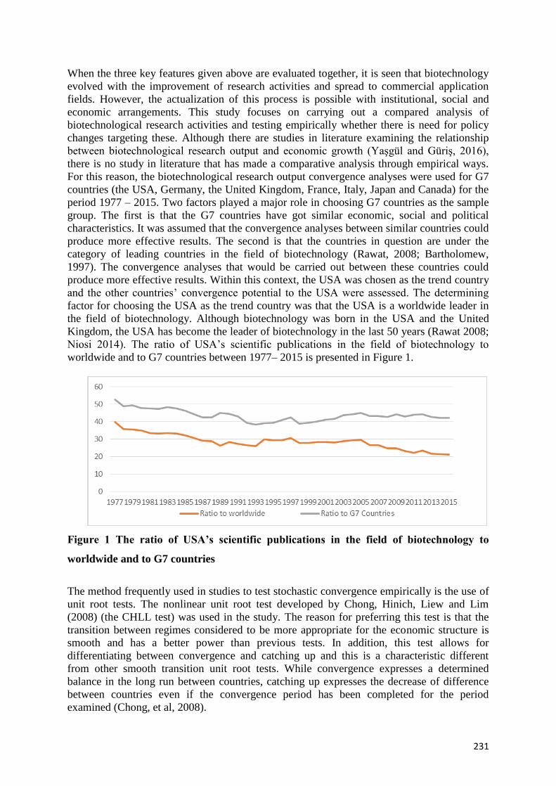
231

When the three key features given above are evaluated together, it is seen that biotechnology

evolved with the improvement of research activities and spread to commercial application

fields. However, the actualization of this process is possible with institutional, social and

economic arrangements. This study focuses on carrying out a compared analysis of

biotechnological research activities and testing empirically whether there is need for policy

changes targeting these. Although there are studies in literature examining the relationship

between biotechnological research output and economic growth (Yaşgül and Güriş, 2016),

there is no study in literature that has made a comparative analysis through empirical ways.

For this reason, the biotechnological research output convergence analyses were used for G7

countries (the USA, Germany, the United Kingdom, France, Italy, Japan and Canada) for the

period 1977 – 2015. Two factors played a major role in choosing G7 countries as the sample

group. The first is that the G7 countries have got similar economic, social and political

characteristics. It was assumed that the convergence analyses between similar countries could

produce more effective results. The second is that the countries in question are under the

category of leading countries in the field of biotechnology (Rawat, 2008; Bartholomew,

1997). The convergence analyses that would be carried out between these countries could

produce more effective results. Within this context, the USA was chosen as the trend country

and the other countries’ convergence potential to the USA were assessed. The determining

factor for choosing the USA as the trend country was that the USA is a worldwide leader in

the field of biotechnology. Although biotechnology was born in the USA and the United

Kingdom, the USA has become the leader of biotechnology in the last 50 years (Rawat 2008;

Niosi 2014). The ratio of USA’s scientific publications in the field of biotechnology to

worldwide and to G7 countries between 1977– 2015 is presented in Figure 1.

Figure 1 The ratio of USA’s scientific publications in the field of biotechnology to

worldwide and to G7 countries

The method frequently used in studies to test stochastic convergence empirically is the use of

unit root tests. The nonlinear unit root test developed by Chong, Hinich, Liew and Lim

(2008) (the CHLL test) was used in the study. The reason for preferring this test is that the

transition between regimes considered to be more appropriate for the economic structure is

smooth and has a better power than previous tests. In addition, this test allows for

differentiating between convergence and catching up and this is a characteristic different

from other smooth transition unit root tests. While convergence expresses a determined

balance in the long run between countries, catching up expresses the decrease of difference

between countries even if the convergence period has been completed for the period

examined (Chong, et al, 2008).

232

The rest of the paper is structured as follows. Section 2 presents the set of data used in the

study and outlines econometric methodology. Section 3 presents empirical findings. Section 4

summarizes the main results of the study and discusses political proposals.

3 Data and Methodology

In this study, it was tested whether research output in biotechnology has converged in G7

countries for the period 1977-2015. The number of scientific publications was used parallel

to literature in order to measure the number of research output in the field of biotechnology

(De Moya-Anegon and Herrero-Solana 1999; Jin 2009; Lee et al. 2011; Inglesi-Lotz and

Pouris 2013; Inglesi-Lotz et al. 2014; Inglesi- Lotz et al. 2013).

The database of The National Science Indicators of Institute for Scientific Information (ISI)

from Thomson Reuters was used to obtain research output. ‘‘Biotechnology and Applied

Microbiology’’ was chosen to find international scientific publications in the field of

biotechnology.

The number of scientific publications in the field of biotechnology in G7 countries for the

period 1977 – 2015 is given in Figure 2. As can be seen in the figure, the USA displayed a

much better performance in the given period than the G7 countries in terms of scientific

publications in the field of biotechnology. For this reason, the convergence analyses used in

the study examine the other G7 countries’ convergence/catching up potentials in comparison

to the USA.

Figure 2 The number of scientific publications in the field of biotechnology in G7

countries

Stochastic convergence was introduced by Carlino and Mills (1993) and Bernard and

Darlauf(1995). According to Bernard and Darlauf (1995), if the logarithm of the analyzed

variable , follows a stationary process, then stochastic convergence occurs.

233

Where is the analyzed variable, is the variable value for unit i at time t and is the

variable value for unit j at time t.

The method frequently used to test stochastic convergence empirically is the use of unit root

tests. The stationarity finding to be obtained in the test expresses convergence. This study

examines the convergence of research output in biotechnology in G7 countries to the USA

and the nonlinear unit root test developed by Chong, Hinich, Liew and Lim (2008) was used.

The reason for preferring these tests is that the transition between regimes considered to be

more appropriate for the economic structure is smooth and has a better power than previous

tests. In addition, the difference of this test is that it allows for differentiation between

convergence and catching up.

Chong, Hinich, Liew and Lim (2008) test is an extended form of unit root test developed by

Kapetanios et al. (2003)(KSS). The test is different from the KSS test as it was developed by

adding the cutting parameter and the trend to the model to be used in the unit root test. It is,

thus, possible to make the differentiation between the convergence and catching up

hypotheses. The equation to be used for the test is as follows:

is the original series to be examined and is the trend variable and this

variable can be in different forms. The trend variables used frequently are linear trend and

nonlinear trend variables. The null hypothesis for nonstationarity is and the

alternative hypothesis for stationarity is . The test statistics is the test statistics of

the parameter as it is the case with the conventional ADF test mentality. Critical values are

tabulated in the study by Chong, Hinich, Liew and Lim (2008).

4. Empirical Findings

This study aims to test whether research output in biotechnology has converged in G7

countries. To achieve this, the CHLL test is used. The results are tabulated in table 1.

Table 1: CHLL Test Results

Lags Test Statistic Trend Coef Trend tstat p value

Germany 0 -5.041079a -0.007211 -0.531017 0.5818 Convergence

France 3 -4.675093a -0.004202 -3.694794 0.0009 Catching-up

United

Kingdom 1 -2.793664c -0.004789 -2.933023 0.006 Catching-up

Italy 2 -3.089871b 0.001408 0.98561 0.3317 Convergence

Japan 0 -2.932801c -0.005403 -2.382878 0.0053 Catching-up

Canada 1 -0.069641 -0.000554 -0.238601 0.8128 Divergence a,b,c Level of significance at the 1, 5 and 10 %, respectively

The significance of the test statistics indicates the rejection of the null hypothesis of no

convergence. In Table 1, unit root is found only for Canada. This means that research output

in biotechnology for Canada has been divergent from the USA. The research output in

biotechnology has been found to converge for other countries. On the other hand, the

significance of the trend parameter will suggest long-run convergence or otherwise the

catching-up hypothesis. It can be seen in Table 1 that the significance of the trend parameter

234

are shown for France, the United Kingdom and Japan. The insignificant trend parameter for

Germany and Italy indicates long run convergence to the USA.

5. Conclusion

In this study, it was aimed to analyze whether research output in biotechnology has

converged in G7 Countries for the period 1977-2015. The number of scientific research

publications in biotechnology was used as research output. With respect to the number of

publications, the USA was taken as the trend country and the other G7 countries’

convergence/catching up potentials in comparison to the USA were analyzed using the CHLL

nonlinear unit root test.

In the light of the obtained findings, while Germany and Italy display long-term convergence

performance, France, the United Kingdom and Japan display catching up performance.

Canada, on the other hand, displays convergence in comparison to the USA’s publication

performance. Therefore, it was concluded that Canada needs a significant change in policy to

increase scientific publications in biotechnology. The question of what these policies

are/could be is beyond the scope of this research. Beyond empirical analyses, more

comprehensive institutional, historical and social analyses are needed to be carried out in

order to answer these questions. The purpose of this study is to determine the current

situation in the light of data and methods available.

Kaynaklar

1. Bartholomew, S.: National Systems of Biotechnology Innovation: complex

interdependence in the global system. J. Int. Bus. Stud. 28(2), 245–246 (1997)

2. Bernard, A. B., & Durlauf, S. N., Convergence in international output, Journal of applied

econometrics, 10(2), 1995, pp 97-108. s.99

3. Carlino, G. and Mills, L. (1993). Are U.S. regional incomes converging? A time series

analysis. Journal of Monetary Economics, Vol. 32, 335-346.

4. Chong, T. T. L., Hinich, M. J., Liew, V. K. S., & Lim, K. P. (2008). Time series test of

nonlinear convergence and transitional dynamics. Economics Letters,100(3), 337-339.

5. De Moya- Anegon, F., Herrero-Solana, V.: Science in America Latina: a comparison of

bibliometric and scientific-technical indicators. Scientometrics 46(2), 299–320 (1999)

6. Evans, P.: Constructing the 21st-century developmental state: potentialities and pitfalls.

In: Edigheji, O. (ed.) Constructing a Democratic Developmental State in South Africa

Potentials and Challenges, pp. 37–58. HSRC Press, Cape Town (2010)

7. Evans, P.: What will the twenty-first century developmental state look like? Implications

of contemporary development theory for the state’s role. In: Wing-kai, S., Wong, S. (eds.)

Repositioning the Hong KongGovernment, pp. 23–44. Hong Kong University Press,

Hong Kong (2012)

8. Ho, R.J., Gibaldi, M.: Biotechnology and Biopharmaceuticals Transforming Proteins and

Genes into Drugs. Wiley-Liss, Wilmington (2003)

9. Inglesi-Lotz, R., Balcılar, M., Gupta, R.: Time-varying causality between research output

and economic growth in US. Scientometrics. 100, 203–216 (2014)

235

10. Inglesi-Lotz, R., Pouris, A.: The influence of scientific research output of academics on

economic growth in South Africa: an autoregressive distributed lag (ARDL) application.

Scientometrics. 95, 129–139 (2013)

11. Inglesi- Lotz, R., Hsieh, C.R., Chang, T., Gupta, R.: Causality between research output

and economic growth in BRICS. Qual. Quant. (2013). doi:10.1007/s11135-013-9980-8

12. Jin, J.C.: Economic research and economic growth: evidence from East Asian Economies.

J. Asian Econ. 20,150–155 (2009)

13. Kapetanios G, Shin Y, Snell A.: Testing for a unit root in the nonlinear STAR framework.

J. Econometrics. 112, 359-379. (2003)

14. Lee, L.C., Lin, P.H., Chuang, Y.W., Lee, Y.Y.: research output and economic

productivity: a Granger causality test. Scientometrics. 89(2), 465–478 (2011)

15. Niosi, J.. (2014). Biotechnology: A case of delayed international convergence? . Int. J.

Biotechnology. 13/1/1/3, 6.

16. Niosi, J., Reid, S.E.: Biotechnology and nanotechnology: science-based enabling

technologies as windowsof opportunity for LDCs? World Dev. 428, 426–438 (2007)

17. Niosi, J., Bas, T.G., Amador, J.F.: Biopharmaceuticals in Latin America: challenges and

opportunities. Innov. Dev. 3(1), 19–36 (2013)

18. Prange, H. & Kaiser, R.. (2004). The Reconfiguration of National Innovation Systems-

The Example of German Biotechnology. Research Policy. 33, 396.

19. Rawat, H.. (2008). Textbook of Biotechnology. Jaipur: Global Media.

20. Rasmussen, B.: Innovation and Commercialisation in the Biopharmaceutical Industry

Creating and Capturing Value. Edgar Elgar Publishing Limited, Cheltenham (2010)

21. Wong, J.H., Chen, T., Tsai, C.: In search of an innovative state: the development of the

state of the biopharmaceutical industry in Taiwan, South Korea and China. Dev. Change

43(2), 481– 482 (2012)

22. Yaşgül, Yaşar Serhat, and Burak Güriş. "Causality between research output in the field of

biotechnology and economic growth in Turkey." Quality & Quantity(2015): 1-12.

236

COMPLEXITY, COMPETITIVENESS AND TECHNOLOGY:

IS THERE A LINK?

Uğur Aytun

Anadolu University, Turkey

Yılmaz Kılıçaslan

Anadolu University, Turkey


Abstract

This study aims to investigate whether complexity, which is a function of locally available

capabilities, has an impact on manufacturing competitiveness that is said to be a vital source

of sustainable economic growth by triggering export and to identify the possible drivers of

complexity. In this study, differently from existing studies, the complexity based on

application of network theory level has been calculated across industry-country level by

using BACI database. Our high dimensional (country, industry and time) fixed effects

estimation results combining UNIDO database for 65 countries for period of 1990-2010 show

that the level of complexity has statistically significant and positive impact on

competitiveness when all industries are included. If we split industries into different

technological categories, however, this impact disappears in low- and medium-low tech

industries, which largely consist of food and beverage, textile and petroleum products, and

increases in medium high and high-tech industries. In addition, we found that average wage,

which is taken into account to test the theory of comparative advantage, has insignificant

impact in all but high-tech industries, being in favor of Kaldor paradox. Finally, for

complexity model, number of establishment, industry-specific human capital, demand and

market structure have been found as significant determinants.

Keywords: Competitiveness, complexity, manufacturing industry.


-237-

1. Introduction

The concept of “Competitiveness” frequently used by businessmen, politicians and

economists originally developed in Business discipline forms basis for strategic analysis of

firms to maximize the profits and to increase market share. In Economics literature, though

the concept serves to various strategies (policies) to reach some objectives such as enhancing

living standards, achieving sustainable development and breaking poverty trap, definitions

may differ in terms of unit in question (country, sector), measurement (exchange rate, labor

costs, trade share, GDP per capita) and period of time (short-run or long-run). These

competitiveness definitions and indicators may be grouped as price (exchange rate, wage,

price level) and non-price (investment, technology, productivity) or “national (GDP per

capita, total export and trade share, balance of payment) and industry (industry trade share

and industry wage level)”. Due to the fact that national- and price-based definitions faced

some criticisms because of ignoring basic mechanisms (scale economies, increasing returns,

and externalities) and assuming structural factors constant, “industry competitiveness”

concept has been developed and refer to strategic industries to improve national

competitiveness and thus, living standards.

It is well-known in the international trade literature that price determinants (exchange rate,

price level, labor costs) do not fully explain the competitiveness levels of countries and

technological efforts are more persuasive. What is little-known is that developing countries

suffering from institutional and market failures, uncertainties and low human capital ratio

have substantial costs in engagement in the efforts and adapting transferred technology. Thus,

they may need industry-selective government interventions to promote industrial capability

base.

In this paper, our methodology is based on two steps. Firstly, we empirically investigated the

of impact technological capabilities on competitiveness at country and country-product level.

Complexity index, which is the application of network analysis and assumed to be function of

the capabilities was calculated by using 1993-2010 BACI bilateral data. This methodology

allows us to see whether industry-specific and nationwide capabilities have an effect on

competitiveness performances of countries. We saw that while industry-specific complexity

effect has been found significant in all industries, this effect is more apparent in medium high

and high-tech industries. However, only country-level complexity impact is significant in

low-tech industries.

Secondly, since the complexity index eventually an ex-post measurement, to see how to

develop capabilities, we tried to identify possible drivers of it. Among them, industry-specific

human capital, demand and market structure have been found as significant determinants.

The paper is organized as fallows: In section 2, we discussed the underlying theoretical and

empirical studies on the link between competitiveness, technology and capabilities. We

introduce how we calculate the nationwide and industry level complexity indices in section 3.

Section 4 and 5 presents some empirical evidence for estimation results for complexity and

competitiveness model by taking into account relative price (unit labor cost) and non-price

determinants (labor productivity and investment intensity). Finally, section 6 concludes and

derives sector-level policy implications.

-238-

2. Competitiveness, technology and capabilities approach

Relation between technology and competitiveness dates back to Leontief (1953)’s seminal

work, showing that unlike the Heckscher-Ohlin’s factor endowment theory, US export rely on

labor intensive products. Although this paradoxical finding was attributed to high labor

productivity in US industries by author, it led to rise of neo-technological trade theories

developed by Posner (1961) and Vernon (1966). According to this argument, probability of

generating new products is higher in industrialized countries because of high labor costs and

purchasing power of its citizens. Inventors will have temporary monopoly profit in their

products’ early stages. However, since firms in follower low-wage countries will imitate these

innovations in later stages, monopolist position in leader country begin to disappear. Length

of this cycle depends on the degree of competition in the market and technological dimension

of innovation (Posner, 1961, pp. 323-331; Vernon, 1966, pp. 200). This argument was found

to be consistent with empirical evidence by selected several studies (Keesing, 1967; Gruber et

al., 1967; Sveikauskas; 1983; Hughes; 1983; Hirsch and Bijaoui, 1985). Keesing (1967, pp.

40-45)’s analysis was based on correlation coefficient between the international

competitiveness and R&D expenditures, and found that R&D activity is highly and

significantly correlated with trade performance.

Gruber et al. (1967, pp. 23-30) also examined the link between the competitiveness of US

exports and R&D expenditures. They found that there is a strong relation between the US

exports and R&D expenditures in the industries having higher share of total US exports when

denominator used as World trade. However, they reached insignificant results when Germany

and United Kingdom were used as benchmark countries. Authors interpreted these findings

with the fact that export profiles of these countries are very similar.

Sveikauskas (1983, pp. 546-550), calculated the net export/consumption ratios of 354 US

industry in 1967. His findings showed that these ratios are higher in industries making higher

R&D expenditure and patenting intensively. Moreover, these sectors contributed to total

productivity in US.

Hughes (1993, pp. 546-550), differently from two studies above, tested the validity of neo-

factor and neo-technological trade theories for 46 UK manufacturing industries in 1978. He

reached that R&D, industry structure and skill level positively related with competitiveness,

according to regression analysis results. However, traditional factor endowments do not have

any effect on export level.

Hirsch and Bijaoui (1985, pp. 247-248) used trade, R&D and size data of Israeli innovative

firms in regression analysis for period 1975-1981. They accepted the product life cycle

hypothesis that the higher R&D intensity is associated with higher propensity to export. They

explained this finding with the fact that every rational firm must reach certain domestic sales

volume to make R&D profitable.

Product life cycle hypothesis has been systematically modeled by Krugman (1979a, pp. 254-

262). According to so-called “product variety” model, international trade is function of

continuous innovation process in North and and transfer of technology toward South. Model

converge to the point that North export new products and South import them. In addition,

North’s success on maintaining high wages was explained by monopolist power over new

products. Slower innovation rate and faster technology transfer would narrow wage gap and

negatively effect the living standards.

-239-

Three theoretical arguments above have been criticized by Lall (2000, pp. 3-8). According to

him, Heckscher-Ohlin theories assume that technological diffusion across firms and countries

is costless and without lags. However, countries with similar factor endowments and even

skill resources can differ in terms of export performances. He also questioned the product life

cycle theories by stating that technology transfer does not necessarily trigger the imitation and

learning process32. Technological capabilities approach, based on the evolutionary tradition of

Nelson and Winter (1982) and modern information theory of Stiglitz (1996, pp. 156), focused

on micro-level learning process in developing countries. Industrial success in these countries

heavily depends on extent to which firms managed to mastering, adapting and improving

process upon existing technologies. However, since this process in developing countries

contain not only basic problems in economy (weak capital markets and institutional structure,

lack information and provision problems) but also market failures, uncertainties, cost, and

risk, governments are called to overcome the market and institutional failures. Furthermore,

these interventions must be selective since every industrial activity has different technology

level and therefore learning processes and externalities (Lall, 2004, pp. 11). Hence, this

approach tries to answer the criticisms above and reconcile technological trade theories with

developing countries’ structural problems.

OECD (1987, pp. 18) illustrates the long term differences in industrialized countries’

performance as follows:

“the best that can be achieved; while incentives guide the use of capabilities

and, indeed stimulate their expansion, renewal or disappearance. In the

advanced economies, capabilities refer primarily to supplies of human capital,

of savings and of existing capital stock, as well as to the technical and

organizational skills, and incentives. Both incentives and capabilities operate

within an institutional framework.”

By using this conceptualization, according to Lall (1992, pp. 170) national technological

capabilities is interplay of human and physical capital, technological efforts, incentives and

institutions. Note that the definition above lies beyond R&D or patenting and see government

policies and institutional structure as important factor to improve the national technological

capabilities, especially in developing countries.

Capabilities, as in the sense above, is measured based on the indexes derived from the trade

data. First of all was “sophistication index” developed by Lall et al. (2005, pp. 8). To obtain

this variable requires to calculate product sophistication first, by multiplying GDP per capita

with share of exports of country in related product. After normalizing the product scores,

country sophistication score is calculated by multiplying the normalized scores with export

share of product and taking weighted average. Lall et al. (2006, pp. 230-232) conducted

descriptive analysis and saw that competitiveness level and sophisticated scores are highly

related.

Hausman et al. (2007) used similar methodology but replaced export share of country with

Balassa’s RCA index when calculating the product sophistication. Their panel regression

analysis found that export sophistication index is positive and significant determinant of

productivity growth.

32 Lall (2000) also stated that lack of new trade theories model of Krugman (1979b, pp. 469) deals trade

between only (mostly industrialized) countries with same characteristics such as tastes, technology and factor endowments. However, since developing countries have localized in different regions, their trade patterns may not be explained with economies of scale.

-240-

Using income information in these measures caused to criticism that rich countries export

rich-country products” (Abdon et al., 2010, 3). Instead, Hidalgo (2009, pp. 5) developed an

“complexity” index by separating income information on income from information on

network structure and used Lego models to be explained below. They also observed positive

and significant effect of complexity on productivity growth (Hidalgo and Hausman, 2009, pp.

10574). Similar results for China at region level have been found by Poncet and Waldemar

(2013).

Abdon et al. (2010, pp. 8-23) calculated the complexity index for countries and products, and

found that countries with high more complex product share in world trade are also those

having high income. In addition, as income grows, export composition of a country moves

toward more complex products.

Karadam ve Ozmen (2015, pp. 25-26)’s paper is on the degree of integration to global value

chains in Turkish manufacturing industries, which is positively correlated with product

complexity index by assumption. Their fixed effect estimation results show positive relation

between product complexity and industry export.

3. Measurement of Complexity Index

As we mentioned above, complexity index is an indirect measure of capabilities by assuming

each capability as Lego model. When we think each product as Lego piece, an individual’s

Lego basket increases as he or she has different Lego pieces thus can build quite different

shapes. Likewise, a country’s capabilities would increase if it is able to export more different

products, especially those that can be exported by less countries which their product

diversification is high. Let formalize these explanations to be more clear.

First of all, we need to calculate the Balassa’s Revealed Comparative Advantage RCA index

for each country and each product (Hidalgo and Hausman, 2009, pp. 10570-10572).

(1)

By using equation (1), we generated vector which is equal to one if is greater than

one and is equal to zero, otherwise. In this way, we connected countries to products when

. Secondly, we aggregated vector for each country and each product. While

former is called diversification , latter is ubiquity .

(2)

(3)

After multiplying with and aggregated for each country (product), we divided

by . This process was iterated “n” times until relative country complexity rankings

remain same. After all, we would have country and product complexity indices:

(4)

(5)

-241-

Finally, we calculated "country-industry specific" complexity index by taking weighted

average of for each country and three-digit manufacturing industry group (j):

(6)

4. The Data

We used three different data sources in this study. Firstly, BACI dataset by Gaulier and

Zignago (2016) collect bilateral data for trade for period 1989-2014. It corrects the raw data

of COMTRADE trade data reconciling the declarations of exporter and importer. Our second

data source is UNIDO (2014) which presents value added, wage, investment and employment

series of countries for manufacturing industry between 1989-2010. Finally, human capital and

natural endowment indices at disaggregated level by Shirotory et al. (2010) has been used in

complexity estimation which will be explained below.

5. Empirical Methodology and Findings

5.1. Competitiveness model

In the first place, we constructed a competitiveness model consisting price and non-price

determinants to find out extent to which complexity has an impact on competitiveness across

different technological intensities. The high-dimensional (country, industry and year) model

which investigates the effect of country-product level complexity is as follows:

(7)

Assuming that subscripts , are country, industry and time, dependent variable is

change in relative export share of country. , , and are relative average wage,

relative investment intensity and relative labor productivity, respectively. Finally, terms ’s

represent country, industry and time dummies and is error term with white noise.

To test the country-level complexity effect, let shows the index value which have 16

iterations, equation (8) is our alternative model:

(8)

Obviously, our variable of interest is and it expected positive for both specifications.

Our first competitiveness estimation results have been presented in Table-1. In the first

column, country-product level complexity has positive and significant coefficient, expectedly.

However, while this variable turned out as insignificant, as technological category moves to

medium- and high-tech industries returns to the industry-specific capability endowment is not

only significant but also higher than the other technology class. Among other variables,

positive and significant coefficient of relative average wage confirms the Kaldor paradox but

this finding contradicts when we estimate within high-tech industries. Relative investment

rate and labor productivity is only significant and expected sign only in all industries and

high-tech industries estimations.

-242-

Table-1: Competitiveness model with country-industry complexity, 1989-2010

(1) (2) (3) (4) (5)

All Low-tech

Medium

low-tech

Medium

high-tech High-tech

VARIABLES

industries

OLS

industries

OLS

industries

OLS

industries

OLS

industries

OLS

0.030** 0.006 0.035 0.076** 0.101*

(0.010) (0.010) (0.034) (0.026) (0.042)

-0.016 0.026+ 0.003 0.021 -0.083**

(0.010) (0.014) (0.027) (0.020) (0.024)

0.005* 0.004 0.006 0.007 0.019**

(0.003) (0.003) (0.007) (0.005) (0.007)

0.015+ -0.004 -0.010 0.014 0.049**

(0.008) (0.013) (0.019) (0.013) (0.015)

Observations 25,887 9,962 5,159 7,028 3,738

R-squared 0.053 0.061 0.042 0.075 0.133

Year Dummies yes yes yes yes yes

Industry Dummies yes yes yes yes yes

Country Dummies yes yes yes yes yes

Robust standard errors in

parentheses

** p<0.01, * p<0.05, + p<0.1

Table-2 shows the effect of country-level complexity on competitiveness and we saw that the

variable of interest is significant for medium high-tech industries again. What is different

from the findings above, general capability structure affects the low-tech and do not so for

high-tech industries. Findings of other variables is found as similar with Table-1.

Table-2: Competitiveness model with country complexity, 1989-2010

(1) (2) (3) (4) (5)

All Low-tech

Medium

low-tech

Medium

high-tech High-tech

VARIABLES

industries

OLS

industries

OLS

industries

OLS

industries

OLS

industries

OLS

0.077** 0.076** 0.038 0.127** 0.082

(0.019) (0.023) (0.053) (0.039) (0.066)

-0.015 0.028* 0.003 0.021 -0.088**

(0.010) (0.014) (0.027) (0.020) (0.024)

0.006* 0.004 0.006 0.007 0.020**

(0.003) (0.003) (0.007) (0.005) (0.007)

0.016* -0.003 -0.010 0.018 0.053**

(0.008) (0.013) (0.019) (0.014) (0.015)

Observations 25,887 9,962 5,159 7,028 3,738

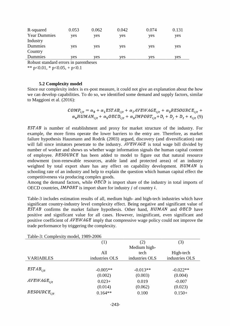
-243-

R-squared 0.053 0.062 0.042 0.074 0.131

Year Dummies yes yes yes yes yes

Industry

Dummies yes yes yes yes yes

Country

Dummies yes yes yes yes yes

Robust standard errors in parentheses

** p<0.01, * p<0.05, + p<0.1

5.2 Complexity model

Since our complexity index is ex-post measure, it could not give an explanation about the how

we can develop capabilities. To do so, we identified some demand and supply factors, similar

to Maggioni et al. (2016):

(9)

is number of establishment and proxy for market structure of the industry. For

example, the more firms operate the lower barriers to the entry are. Therefore, as market

failure hypothesis Hausmann and Rodrik (2003) argued, discovery (and diversification) rate

will fall since imitators penetrate to the industry. is total wage bill divided by

number of worker and shows us whether wage information signals the human capital content

of employee. has been added to model to figure out that natural resource

endowment (non-renewable resources, arable land and protected areas) of an industry

weighted by total export share has any effect on capability development. is

schooling rate of an industry and help to explain the question which human capital effect the

competitiveness via producing complex goods.

Among the demand factors, while is import share of the industry in total imports of

OECD countries, is import share for industry of country .

Table-3 includes estimation results of all, medium high- and high-tech industries which have

significant country-industry level complexity effect. Being negative and significant value of

confirms the market failure hypothesis. Other hand, and have

positive and significant value for all cases. However, insignificant, even significant and

positive coefficient of imply that compressive wage policy could not improve the

trade performance by triggering the complexity.

Table-3: Complexity model, 1989-2006

(1) (2) (3)

All

Medium high-

tech High-tech

VARIABLES industries OLS industries OLS industries OLS

-0.005** -0.013** -0.022**

(0.002) (0.003) (0.004)

0.023+ 0.019 -0.007

(0.014) (0.062) (0.023)

0.164** 0.100 0.150+

-244-

(0.041) (0.098) (0.088)

1.591** 1.597** 2.831**

(0.065) (0.123) (0.189)

21.615** 17.159** 4.350*

(0.877) (1.885) (1.989)

0.000 0.002** -0.000

(0.000) (0.001) (0.000)

Observations 36,842 10,209 5,362

R-squared 0.826 0.698 0.673

Year Dummies yes yes yes

Industry Dummies yes yes yes

Country Dummies yes yes yes

Adjusted R-square 0.825 0.694 0.666

Robust standard errors in parentheses

** p<0.01, * p<0.05, + p<0.1

6. Conclusion

What countries export is not simply determined by different combinations of inputs, as

traditional trade theories claim. Choosing which product to be exported is a function of

capabilities which are specific inputs that locally available. Moreover, these capabilities can

be industry specific because some industrial activities have different technology level, and

therefore learning processes and externalities.

In this study, we constructed a competitiveness model to test the impact of country-industry

level complexity index. We found that returns to industry-specific complexity in terms of

trade share in technology intensive industries are higher. On the other hand, trade

performance of traditional industries can be improved only through general capability

structure of countries. Put it differently, competitiveness performance of low-tech industries is

determined by all industries' complexity structure. Penetration of new technologies to these

industries can help their competitiveness.

We also found that developing capabilities requiring industry-specific focus, which are

technology intensive industries and highest trade share in our case, depends primarily on

industry specific human capital content, being consistent with Costinot (2009) and Maggioni

et al. (2016). However, even though compressive wage policies contributed to

competitiveness in some scenarios, these could not have specific effect on complexity that

could provide sustainable and healthy trade performance.

Barriers to entry in the industry of an economy may be detrimental to the diversification, as

market failure hypothesis argued. However, when considering the inter-spillover effects and

importance of diversification in developing countries, to protect the industry should not be

used as industry policy. Instead, first-mover entrepreneurs can be supported (Rodrik, 2004).

Finally, demand structure of high income countries should be followed because their

preference set is used as escalator to develop capabilities.

To conclude, we suggest that countries should concentrate on nationwide and industry

specific capability building. However, governance and free-trade policies offered by

-245-

mainstream trade theories are inadequate in this process. Especially for developing countries,

governments may overcome the market failures, information asymmetries and coordination

problems in directing resources by establishing new institutions and agencies that handles the

education (or training), competition and supervision policy at industry level.

References

1. Abdon, A., Bacate, M., Felipe, J., & Kumar, U. (2010). Product Complexity and Economic

Development. Working Paper No. 616, Levy Economics Institute of Bard College.

2. Boltho, A. (1996). The assessment: international competitiveness. Oxford Review of

Economic Policy, 12 (3), 1-16

3. Fagerberg, J. (1996). Technology and Competitiveness. Oxford Review of Economic Policy,

12 (3), 1-16

4. Fagerberg, J. (1988). International Competitiveness. The Economic Journal, 98 (391), 355-

374.

5. Gaulier, G., & Zignago, S. (2016) BACI: International Trade Database at the Product-Level.

The 1989-2014 Version. CEPII Working Papers.

6. Gruber, W., Mehta, D., & Vernon, R. (1967). The R & D Factor in International Trade and

International Investment of United States Industries. Journal of Political Economy, 75 (1),

20-37.

7. Hausmann, R., & Hidalgo, C. A. (2010). Country diversification, product ubiquity, and

economic divergence. CID Working Paper No. 201, Center for International Development at

Harvard University.

8. Hausmann, R., & Hidalgo, C. A. (2011). The network structure of economic output. Journal

of Economic Growth, 16, 309-342.

9. Hidalgo, C. A. (2009). The Dynamics of Economic Complexity and the Product Space over a

42 year period. CID Working Paper No. 189, Center for International Development at

Harvard University.

10. Hidalgo, C. A., & Hausmann, R. (2009). The building blocks of economic complexity.

Proceedings of the National Academy of Sciences, 106 (26), 10570-10575.

11. Hidalgo, C. A., Klinger, B., Barabasi, A. -L., & Hausmann, R. (2007). The Product Space

Conditions the Development of Nations. Science, 317, 482-487.

12. Hirsch, S., & Bijaoui, I. (1985). R&D intensity and export performance: A micro view.

Weltwirtschaftliches Archiv, 121 (2), 238-251.

13. Hughes, K. S. (1993). Introduction: internationalization, integration and European

competitiveness. In K. S. Hughes, European competitiveness. Cambridge: Cambridge

University Press.

14. Kaldor, N. (1978). Further Essays on Applied Economics. New York, United States: Holmes

and Meier.

15. Karadam, D. Y., & Özmen, E. (2015). Teknolojik Yetkinlik ve Türkiye Dış Ticareti. İktisat

İşletme ve Finans, 30 (357), 9-34.

16. Keesing, D. B. (1967). The Impact of Research and Development on United States Trade.

Journal of Political Economy, 75 (1), 38-48.

17. Kilicaslan, Y., & Aytun, U. (forthcoming). Product Life Cycle and Innovativeness: The Case

of MENA.

18. Krugman, P. (1979a). A Model of Innovation, Technology Transfer, and the World

Distribution of Income . Journal of Political Economy, 87 (2), 253-266.

-246-

19. Krugman, P. (1979b). Increasing returns, monopolistic competition, and international trade.

Journal of International Economics, 9 (4), 469-479.

20. Lall, S. (1992). Technological Capabilities and Industrialization. World Development, 20 (2),

165-186.

21. Lall, S. (2000). Turkish Performance in Exporting Manufactures: A Comparative Structural

Analysis. QEH Working Paper Series QEHWPS47, Queen Elizabeth House.

22. Lall, S. (2001). Competitiveness indices and developing countries: an economic evaulation of

the Global Competitiveness Report. World Development , 29 (9), 1501-1525.

23. Lall, S., Weiss, J., & Zhang, J. (2006). The ‘‘Sophistication’’ of Exports: A New Trade

Measure. World Development, 34 (2), 222-237.

24. Lall, S., Weiss, J., & Zhang, J. (2005). The ‘Sophistication’ Of Exports: A New Measure Of

Product Characteristics. QEH Working Paper Series – QEHWPS 123, Quenn Elizabeth

House, Oxford.

25. Leontief, W. (1953). Domestic Production and Foreign Trade; The American Capital

Position Re-Examined. Proceedings of the American Philosophical Society, 97 (4), 332-349.

26. Nelson, R. R., & Winter, S. G. (1982). An Evolutionary Theory of Economic Change.

Cambridge, Massachusetts: The Belknap Press of Harvard University Press.

27. Maggioni, D., Turco, A., & Gallegati, M. (2016). Does Product Complexity Matter for

Firms’ Output Volatility? Journal of Development Economics, 121, 94-109

28. OECD. (2011). ISIC Rev.3 Technology Intensity Definition: Classification of manufacturint

industries into caregories based on R&D intensities. OECD Publication, OECD Directorate

for Science, Technology and Industry, Economic Analysis and Statistics Division, Paris.

29. OECD. (1987). Structural Adjustment and Economic Performance. Paris: OECD.

30. Posner, M. V. (1961). International Trade and Technical Change. Oxford Economic Papers,

13 (3), 323-341.

31. Poncet, S., Starosta, F., & Waldemar, F. (2013). Export Upgrading and Growth: The

Prerequisite of Domestic Embeddedness. World Development, 51, 104-118.

32. Rordik, D. (2004). Industry Policy for Twenty-first Century. Centre for Economic Policy

Research: London

33. Hausmann, R., & Rodrik, D. (2003). Economic Development as Self-Discovery. Journal of

Development Economics, 72, 603-633

34. Sahan, F. (2012). The Impact of Technology Level and Structural Change of Exports on the

Dynamics of International Competitiveness: A Sectoral Disaggregated Analysis of Turkish

Manufacturing Sector. MSc. Thesis, METU, Department of Economics, Ankara.

35. Shirotory, M., Tumurchudur, B., & Cadot, O. (2010). Revealed Factor Intensity Indices at

The Product Level. UNCTAD Blue Series Papers 44. United Nations Conference on Trade

and Development

36. Stiglitz, J. (1996). Some Lessons from the East Asisan Miracle. The World Bank Research

Observer , 11 (2), 151-177.

37. Sveikauskas, L. (1983). Science and Technology in United States Foreign Trade. The

Economic Journal, 93 (371), 542-554.

38. United Nations Industrial Development Organization. (2014). INDSTAT4 2010 ISIC Rev.3.

39. United Nations. (2014). UN comtrade database. New York, United Nations.

40. Vernon, R. (1966). International Investment and International Trade in the Product Cycle.

The Quarterly Journal of Economics, 80 (2), 190-207.

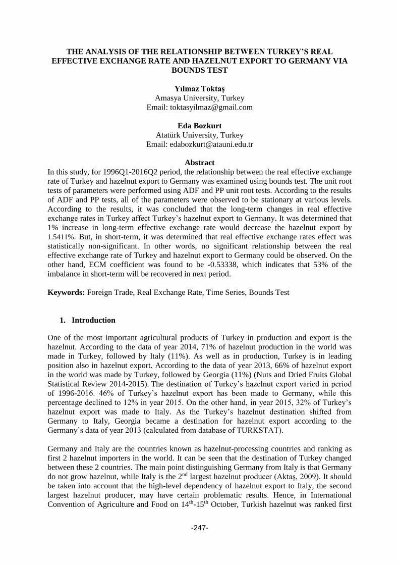
-247-

THE ANALYSIS OF THE RELATIONSHIP BETWEEN TURKEY’S REAL

EFFECTIVE EXCHANGE RATE AND HAZELNUT EXPORT TO GERMANY VIA

BOUNDS TEST

Yılmaz Toktaş

Amasya University, Turkey


Eda Bozkurt

Atatürk University, Turkey


Abstract

In this study, for 1996Q1-2016Q2 period, the relationship between the real effective exchange

rate of Turkey and hazelnut export to Germany was examined using bounds test. The unit root

tests of parameters were performed using ADF and PP unit root tests. According to the results

of ADF and PP tests, all of the parameters were observed to be stationary at various levels.

According to the results, it was concluded that the long-term changes in real effective

exchange rates in Turkey affect Turkey’s hazelnut export to Germany. It was determined that

1% increase in long-term effective exchange rate would decrease the hazelnut export by

1.5411%. But, in short-term, it was determined that real effective exchange rates effect was

statistically non-significant. In other words, no significant relationship between the real

effective exchange rate of Turkey and hazelnut export to Germany could be observed. On the

other hand, ECM coefficient was found to be -0.53338, which indicates that 53% of the

imbalance in short-term will be recovered in next period.

Keywords: Foreign Trade, Real Exchange Rate, Time Series, Bounds Test

1. Introduction

One of the most important agricultural products of Turkey in production and export is the

hazelnut. According to the data of year 2014, 71% of hazelnut production in the world was

made in Turkey, followed by Italy (11%). As well as in production, Turkey is in leading

position also in hazelnut export. According to the data of year 2013, 66% of hazelnut export

in the world was made by Turkey, followed by Georgia (11%) (Nuts and Dried Fruits Global

Statistical Review 2014-2015). The destination of Turkey’s hazelnut export varied in period

of 1996-2016. 46% of Turkey’s hazelnut export has been made to Germany, while this

percentage declined to 12% in year 2015. On the other hand, in year 2015, 32% of Turkey’s

hazelnut export was made to Italy. As the Turkey’s hazelnut destination shifted from

Germany to Italy, Georgia became a destination for hazelnut export according to the

Germany’s data of year 2013 (calculated from database of TURKSTAT).

Germany and Italy are the countries known as hazelnut-processing countries and ranking as

first 2 hazelnut importers in the world. It can be seen that the destination of Turkey changed

between these 2 countries. The main point distinguishing Germany from Italy is that Germany

do not grow hazelnut, while Italy is the 2nd largest hazelnut producer (Aktaş, 2009). It should

be taken into account that the high-level dependency of hazelnut export to Italy, the second

largest hazelnut producer, may have certain problematic results. Hence, in International

Convention of Agriculture and Food on 14th-15th October, Turkish hazelnut was ranked first

-248-

in list of most dangerous imported foods by Coldiretti, the Italian Association of

Agriculturists (http://www.bbc.com/turkce/haberler-dunya-37672069).

It should be considered that the loss of Germany, where there is no supply of hazelnut, to

Georgia, which is the first competitor in export, would have possible negative effects on

Turkey’s hazelnut export in future. The share of Germany in Turkey’s annual hazelnut export

is presented in Figure 1.

Figure 1. The share of Germany in Turkey’s annual hazelnut export

As seen in Figure 1, the share of Germany in Turkey’s annual hazelnut export shows

downwards trend. Germany is an important market as non-producer important and processor

and 2nd largest importer in the world. In present study, the relationship between the hazelnut

export of Turkey to Germany, which is a globally important market, and the real affective

exchange rate was investigated.

In literature, there are many studies discussing the relationship between the exportation and

the exchange rate. Moreover, there also are studies examining the relationship between

agricultural product exportation and foreign exchange rates in addition to the general foreign

trade and exchange rate relationship. Among the agricultural products, the number of studies

examining the relationship of hazelnut export with exchange rate is limited, there are some

examples. Erdal (2008) has examined the relationship of Turkey’s hazelnut export prices with

exchange rate and European Hazelnut Exchange Prices in period of 1995-2007 by using

Johansen Cointegration and Granger Causality tests. According to the cointegration test

results, it was determined that there was a long-term relationship between the series.

According to the causality test, on the other hand, there are one-way relationship form

exchange rate to Turkey’s hazelnut exchange prices and European Hazelnut Exchange prices

and two-way relationship between Turkey’s hazelnut exchange prices and European Hazelnut

Exchange prices.

Hatırlı et al. (2008), in their study employing the monthly data of 1996-2006 period, have

examined the permeability of hazelnut prices from Turkey to Germany by using the two-way

logarithmic model and the exchange rate fluctuations by using GARCH approach. According

to the model estimation results, the price permeability and exchange rate elasticities were

found to be low in short and long-term, and the permeability was determined to be not

complete.

-249-

Akal (2009) has examined the Turkey’s domestic hazelnut export for 1978-2001 period by

using simple econometric and autoregressive averages cause-effect techniques (ARMAX).

The exchange rate elasticity of domestic hazelnut export was found to be inelastic, while the

domestic hazelnut export amount elasticity of export incomes was found to be elastic. In

estimations based on these models, it has been predicted that the domestic hazelnut export and

incomes would increase.

Yanıkkaya et al. (2013) have investigated the effects of exchange rate and exchange rate

fluctuations on the export of, in addition to the hazelnut, certain agricultural products of 46

countries including Turkey for 1971-2010 period. According to the analysis results, no

statistical relationship could be determined between the agricultural product export and

exchange rate fluctuation, while a statistically significant relationship has been found with the

exchange rate.

In his study, Toktaş (2016) has examined the relationship between Turkey’s real effective

exchange rates and its hazelnut export to EU-member countries for 1997Q1-2015Q3 period

by using bounds test. In that study, it has been reported that 1% increase in real effective

exchange rates decreased Turkey’s hazelnut export to EU countries by 2.47%.

In present study, the relationship between Turkey’s hazelnut export and real effective

exchange rates was investigated. Following the “Introduction” section including general

introductive information and a short literature review, the empirical analysis is presented. The

relationship between Turkey’s hazelnut export and real effective exchange rate was tested

using quarterly data for the period of 1996-2016 via bounds test. And then, the paper is ended

with conclusion section.

2. Empirical Analyses

The variables used in this study are Turkey’s real hazelnut export to Germany, real effective

exchange rates, and Germany’s real gross domestic product. The quarterly data covers the

period between the first trimester of 1996 and the second trimester of 2016. The algorithms of

series were cleansed from the seasonality.

Table 1. Variables used in present study

Abbreviation of

Variable

Definition Period Source

LNREXP Turkey’s hazelnut

export to Germany

1996Q1-2016Q2 TURKSTAT database

LNRGDP Germany’s real gross

domestic product

1996Q1-2016Q2 EUROSTAT

LNREER Real effective

exchange rates

1996Q1-2016Q2 BIS

In present study, the foreign trade model used in studies of Bahmani-Oskooee and Goswami

(2004) was employed in order to examine the relationship between export and real effective

exchange rates:

(1)

For Cointegration Analysis, there are cointegration tests in literature used by Engel and

Granger (1987), Johansen (1988), Johansen and Juselius (1990). These tests cannot be used in

cases of various levels of stationarity of variables. The bounds test developed by Paseran et al.

-250-

(2001) allows the cointegration analysis in case of various levels of stationarity of variables.

For the bounds test, the unlimited error correction model (UECM) should be used at first. The

version of UECM modified to present model is presented in Eq.2 below.

(2)

where, t represents trend variable and p indicates the number of lag. In present study, the

length of lag with lowest Schwarz Bayesian Information Criteria (SBC) was considered the

length of lag. In order to test the presence of cointegration relationship, F test is applied to

first period lags of dependent and independent variables. For this test, the null hypothesis is

H0:α4=α5=α6=0. The F-statistic values calculated as a result of the test are compared to top

and bottom limits in Pesaran’s (2001) table. If the calculated F statistics is higher than the top

critical limit of table, then it indicates the presence of cointegration relationship, while the

values lower than bottom limit of table indicate the absence of cointegration relationship. In

case of F values calculated to be within the range between top and bottom critical limits, no

exact interpretation regarding the cointegration relationship can be made (Karagöl, Erbaykal

and Ertuğrul, 2007). After determining the cointegration relationship between the series, then the ARDL

(Autoregressive Distribution Lag) model was established in order to investigate the long- and

short-term relationships between the hazelnut export and real effective exchange rates. The

ARDL model used in present study is shown in Eq.(3):

where, the optimal lengths of lag determined according to SBC are represented with “n, r, s’’.

3. Analysis Results

The stationarity analysis of the series used in present study was tested using ADF

(Augmented Dickey-Fuller) and PP (Phillips Perron) tests. The results of ADF and PP unit

root tests are presented in Table 2. The null hypotheses of ADF and PP test equations are

established based on the assumption that the series includes unit root.

Table 2. Results of ADF and PP Unit Root Tests

Variable

ADF PP

Constant Constant

and Trend Constant

Constant

and Trend

LNREXP Level

t-statistics -3.843608* -5.436865* -3.627029* -5.468792*

1% -3.513344 -4.075340 -3.513344 -4.075340

5% -2.897678 -3.466248 -2.897678 -3.466248

-251-

10% -2.586103 -3.159780 -2.586103 -3.159780

LNRGDP Level

t-

statistics -1.822329 -1.776187

-1.513329 -1.434614

1% -3.521579 -4.086877 -3.521579 -4.086877

5% -2.901217 -3.471693 -2.901217 -3.471693

10% -2.587981 -3.162948 -2.587981 -3.162948

First

Difference

t-

statistics -6.249228*

-

6.216397*

-

6.295111* -6.263475*

1% -3.521579 -4.086877 -3.521579 -4.086877

5% -2.901217 -3.471693 -2.901217 -3.471693

10% -2.587981 -3.162948 -2.587981 -3.162948

LNREER Level

t-

statistics -3.017444**

-

3.292062***

-

2.973639**

-

3.292062***

1% -3.521579 -4.086877 -3.521579 -4.086877

5% -2.901217 -3.471693 -2.901217 -3.471693

10% -2.587981 -3.162948 -2.587981 -3.162948 * indicates significance level of 1%

** indicates significance level of 5%

*** indicates significance level of 10%

In proportion to ADF and PP tests, since the t-statistic calculated for LNREXP and LNREER

series in levels are higher in terms of absolute value, series are stationary, which means that

LNREXP and LNREER series are I(0). The t-statistic values calculated for LNRGDP series in

levels was found to be lower than critical values in table in proportion to ADF and PP tests in

terms of absolute values, while it was found to be higher than critical table values in first

differences. It means that, in proportion to ADF and PP tests, LNRGDP series is stationary at

first difference, thus LNRGDP series is I(1).

The maximum length of lag in present study was taken to be 8, and the number of lag was

determined to be 1 according to SBC. After determining the optimal length of lag regarding

the unlimited error correction model, then the cointegration relationship between the variables

was examined using bounds test. The results of bounds test are presented in Table 3.

Table 3. Bounds test results

Bounds Test Critic Limits

F Statistic = 6.9555 Bottom Limit Top Limit

5% 3.9502 4.9842

10% 3.2740 4.2477

According to Table 3, the F-statistic value which is calculated was found to be 6.9555; since it

is higher than top critical limits of table, the cointegration relation between the variables was

determined. After determining the cointegration relationship, the coefficients of long-term

relationship based on ARDL model were calculated. The estimation of ARDL (1,0,0) model

is presented in Table 4.

-252-

Table 4. Long-term ARDL Model Estimations (1,0,0)

Regressor Coefficient Standard Error T-Ratio[Prob]

LNREXP(-1) 0.46662 0.11007 4.2394[0.000]

LNREER -0.82197 0.49518 -1.6600[0.101]

LNRGDP 0.45618 0.36712 1.2426[0.218]

INPT 6.8019 6.6289 1.0261[0.308]

Definitive Tests Statistics

A:Serial Correlation 1.8471[0.764]

B:Functional Form 10045[0.751]

C:Normality 33.4232[0.000]

D:Heteroscedasticity 16837[0.682]

A: Lagrange multiplier test of residual serial correlation

B:Ramsey's RESET test using the square of the fitted values

C:Based on a test of skewness and kurtosis of residuals

D:Based on the regression of squared residuals on squared fitted

values

In Figure 2, the CUSUM and CUSUMQ test results indicting the consistency of model

are presented. As a result of CUSUM and CUSUMSQ tests, it was determined that the

residuals of model were found to be within the limits, and that the parameters were

consistent.

-0.4

-0.2

0.0

0.2

0.4

0.6

0.8

1.0

1.2

1.4

1998Q1 2002Q4 2007Q3 2012Q2 2016Q2

The straight lines represent critical bounds at 5% significance level

Plot of Cumulative Sum of Squares of Recursive Residuals

-30

-20

-10

0

10

20

30

1998Q1 2002Q4 2007Q3 2012Q2 2016Q2

The straight lines represent critical bounds at 5% significance level

Plot of Cumulative Sum of Recursive Residuals

Figure 1. Plot of Cusum of Squares and Cusum Tests

Long-term coefficients calculated using ARDL (1,0,0) model are presented in Table 5.

Table 5. Long-term Coefficients of ARDL(1,0,0) Model

Estimated Equilibrium LNREXP = f(LNREER, LNRGDP)

Regressor Coefficient T-Ratio[Prob]

LNREER -1.5411 -1.9306[0.058]

LNRGDP 0.85527 1.2263[0.224]

INPT 12.7525 1.1002[0.275]

According to the results of estimations of ARDL model in Table 5, the coefficients of

LNREER and LNRGDP variables are non-significant at significance level of 5%. At

-253-

significance level of 10%, significant and negative relationship between LNREER and

LNREXP was determined. 1% increase in LNREER decreases LNREXP by 1.5411%.

The estimations about short-term relationship via ARDL method based on error correction

model are presented in Table 6.

Table 6. Results of Error Correction Model based on ARDL (1,0,0) Approach

Dependent variable is dLNREXP

Regressor Coefficient T-Ratio[Prob]

dLNREER -0.82197 -1.6600[0.101]

dLNRGDP 0.45618 1.2426[0.218]

ecm(-1) -0.53338 -4.8459[0.000]

Given the ECM coefficient, it can be seen that the value of coefficient is negative and

significant as expected. ECM indicates that 53% of an imbalance in short-term will be

recovered in next period. At significance levels of 5% and 10%, dLNRGDP and dLNREER

are statistically non-significant.

4. Conclusion

The relationship between the Turkey’s hazelnut export to Germany and real effective

exchange rates was examined using quarterly data for the period of 1996-2016. First of all, the

stationarity of series was examined. For the stationarity analyses, the ADF and PP tests

frequently used in literature were utilized; according to the results of stationarity analyses,

LNREER and LNREXP series were found to be I(0) and LNRGDP series was found to be

I(1). Following the stationarity analysis, the cointegration relationship between the series

being stationary at different levels was examined using bounds test developed by Peseran et

al. (2001). According to the bounds test results, a cointegration relationship was found

between the Turkey’s hazelnut export to Germany and real effective exchange rates.

Finally, by using ARDL method, the short- and long-term relationships between Turkey’s

hazelnut export to Germany and real effective exchange rates were analyzed. According to the

results of ARDL model, as expected, real effective exchange rates negatively and

significantly (at significance level of 10%) affects the Turkey’s hazelnut export to Germany in

long-term. The long-term coefficient of real effective exchange rates was found to be -1.5411

at significance level of 10%. It means that 1% increase in real effective exchange rates in

long-term will decrease the hazelnut export by 1.5411%. In short-term, however, the

coefficient of real effective exchange rates at significance levels of 5% and 10% were found

to be statistically non-significant meaning that there is no significant relationship between real

effective exchange rates and hazelnut export to Germany. ECM coefficient was found to be

negative and statistically significant. ECM coefficient of -0.53338 means that 53% of

imbalance in short-term will be recovered in next period.

Determination of the effects of exchange rate policies on the destination change in Turkey’s

hazelnut export is the subject of another study. But, under the lights of empirical results

obtained in present study, it might be concluded that the under-valued exchange rate policy

would be useful in increasing the Turkey’s hazelnut export to Germany. It should be remarked

that the real effective exchange rate is not the sole factor of export, and other factors

influencing the export should be considered while determining the policy to increase the

-254-

export. In present study, it is aimed to provide the policy-makers with more detailed

information regarding the effects of real effective exchange rates on the export through the

example of hazelnut export to Germany.

REFERENCES

1. Akal, M. (2009), “Estimation of Hazelnut Export of Turkey And Forecast Accuracies”,

ZKÜ Sosyal Bilimler Dergisi, 5(10), 77–96.

2. Aktaş, A.R., Öztürk E. and Hatırlı S.A (2009), ‘‘Dünya Fındık Piyasasında Türkiye'nin

Rolü’’ Süleyman Demirel Üniversitesi Vizyoner Dergisi, Cilt 1, Sayı 1,36-54.

3. Bahmani-Oskooee, M. ve Goswami, G.G. (2004), ‘‘Exchange rate sensitivity of Japan’s

bilateral trade flows’’. Japan and the World Economy, 16, 1–15.

4. Erdal, G. ve Uzunöz, M. (2008), “Türkiye ve Avrupa Fındık Fiyatları ve Döviz Kuru

Arasındaki Nedensellik İlişkisi”, U. Ü. Ziraat Fakültesi Dergisi, 22(2), 47-56.

5. Hatırlı, S. A., Öztürk, E. ve Aktaş, A. R. (2008), “Fındık Piyasasında Fiyat

Geçirgenliğinin Analizi”, Akdeniz Üniversitesi Ziraat Fakültesi Dergisi, 21(1),139–143.

6. İtalya'da en tehlikeli gıdalar listesinde Türk fındığı ilk sırada, (2016, October 16).

Retrieved 2016, October 20 from http://www.bbc.com/turkce/haberler-dunya-37672069

7. Nuts and Dried Fruits Global Statistical Review 2014-2015. (2016, October 5). Retrieved

from https://www.nutfruit.org/wp-continguts/uploads/2015/11/global-statistical-review-

2014-2015_101779.pdf

8. Pesaran, M. H., Shin, Y. ve Smith, R. J. (2001), “Bounds testing approaches to the

analysis of level relationship’’, Journal of Applied Econometrics, 16, 289–326.

9. Türkiye İstatistik Kurumu Veri Tabanı, Retrieved 2016, October 7 from

http://www.tuik.gov.tr/PreTabloArama.do?metod=search&araType=vt

10. Toktaş, Y., (2016), Döviz Kuru ve Döviz Kuru Oynaklığının Türkiye’nin Avrupa

Birliği’ne Olan Tarımsal İhracatı Üzerindeki Etkisinin Belirlenmesi, Yayınlanmamış

Doktora Tezi, Sosyal Bilimler Enstitüsü, Erzurum.

11. Yanıkkaya, H., Kaya, H. ve Koçtürk, O. M. (2013), “The Effect of Real Exchange Rates

and their Volatilities on the Selected Agricultural Commodity Exports: A Case Study on

Turkey, 1971–2010”, Agric. Econ. - Czech, 59(5), 235–245.

http://www.bbc.com/turkce/haberler-dunya-37672069

https://www.nutfruit.org/wp-continguts/uploads/2015/11/global-statistical-review-2014-2015_101779.pdf

https://www.nutfruit.org/wp-continguts/uploads/2015/11/global-statistical-review-2014-2015_101779.pdf

http://www.tuik.gov.tr/PreTabloArama.do?metod=search&araType=vt

-255-

THE RELATIONSHIP OF CO2 EMISSION AND ECONOMIC GROWTH IN BRICS-

T COUNTRIES: A PANEL DATA ANALYSIS

Zeynep Karaçor



Duygu Baysal Kurt



Abstract

In this study, in order to study the relationship between economic growth and CO2 emission,

using the data of economic growth, CO2 emission, and energy use of BRICS - T countries

(Brazil, Russia, India, China, South Africa, and Turkey), according to Pooled Mean Group

Estimator-PMGE, it was found that both long and short term parameters of energy use and

GDP were significant. In long term, an increase of 1 % in energy use and GDP raises CO2 in

the rates of approx. 1.22% and 1.13%, respectively. In short term, these coefficients ranges in

0.34% and 0.55%. The results of Dumitrescu Hurlin general causality test points out that there

is a two way relationship between all variables.

Keywords: Economic Growth, CO2 Emission, BRICS - T Countries

1. INTRODUCTION

In 1960s, featuring the negative aspects of economic growth such as pollution, urban severity,

crowdedness, and other negative externalities, they became interest focus. However, as a

result of continuation of high rate economic growth, Rome Club introduced the discussion

“Limits of Growth” regarding that extinctions may be experienced in resources. In this study

of Rome Club, it was emphasized that economic growth should be slowed down (Bruvoll and

Medin, 2003: 27-28).

World Commission on Environment and Development Commission within United Nation

published the report titled “Our Common Future”, in which the interrelation of environment

and development is examined, in 1983. This report emphasized the points such as eliminating

poverty, equally distribution of benefit obtained from natural resources, population control,

struggle with pollution, and use of environmental friendly technology that are necessary to be

able to provide sustainable development (Yenigün, 2011).

Especially since the early 1990s, climatic changes, global warming, and environmental

deterioration have become a common issue. While the emission of CO2 gas is indicated as the

cause of environmental deterioration, the relationship between the gas of interest and

economic growth has formed a contradictive state (Arı and Zeren 2011: 37).

The view that environmental pollution will increase along with economic growth and that it

will decrease after reaching a certain income level is termed as Environmental Kuznets Curve

in the literature (Başar and Temurlenk, 2007: 1). Environmental Kuznets Curve, formed by

Kuznets (1955) based on economic growth and income inequality, was shaped in the light of

the study of Krueger (1991) examining the relationship between air quality and economic



-256-

growth as well as the study of Grossman and Krueger (1995) revealing the relationship

between income and various environmental indicators.

In the study, in order to reveal the relationship economic growth and CO2 emission, literature

was reviewed and dynamic panel data analysis covering the period of 1990-2011 was

conducted on BRICS – T (Brazil, Russia, India, China, South Africa, and Turkey) countries.

2. LITERATURE

Begum et al. (2015), in Malaysia, in order to reveal the effect of economic growth, energy

consumption, and population increase on CO2 emissions, carried out an econometric analysis.

Analyses results indicated that in the period of 1970-1980, the decrease in CO2 per capita and

increase in economic growth were experienced, while in the period of 1980 -2009, an increase

in CO2 emission as well as economic growth occurred. In addition, it was concluded that

while in the long period, there was positive effect of energy consumption and economic

growth on CO2 emission, the same effect was not of interest on population increase.

Joo et al. (2015), in Chili, for the period of 1965-2010, studied the causality relationship

between energy consumption, CO2 emission, and economic growth, utilizing time series

analysis. As a result of analysis, it emerged that there was one directional causality from CO2

emission to economic growth.

Magazzino (2015), dealing with the period of 1971-2006, attempted to reveal the relationship

between economic growth, energy use, and CO2 emission for Israel. According to the

causality results, it was suggested that real gross domestic product caused both to energy use

and CO2 emission.

Aytun (2014), for the period of 1971-2010, studied the relationship between CO2 emission,

economic growth, energy consumption, and educational level in 20 countries by means of co-

integration and panel vector error correction model. The results obtained showed that the

shape of Environmental Kuznets Curve was in the form of inverse U. In addition, in the long

period, it was revealed that there was a causality from the rates of economic growth, energy

use, and schooling to CO2 emission

Gao and Zhang (2014), in order to reveal the relationship between electricity consumption,

economic growth, and CO2 emission, applied the methods of panel co-integration and panel

vector error correction modelling to a group consisting of 14 Sub-Saharan Countries for the

period of 1980-2009. The findings showed that the shape of Environmental Kuznets Curve

was in the form of inverse U: In addition, according to the causality tests, it emerged that

there was the bidirectional relationship between economic growth and CO2 emission.

Lee and Brahmasrene (2014), in order to reveal the relationships between communication

technologies, CO2 emission, and economic growth, using the data belonging to the period of

1991-2009 of 9 countries member to ASEAN, carried out panel data analysis. In the analysis

results showed that there was a long termed equilibrium relationship between the variables. In

addition, it was suggested that besides that there was an opposite directional strong

relationship between CO2 emission and economic growth, there was also the bidirectional

relationship.

Omri et al. (2014), utilizing the data belonging to 54 countries, for the period of 1990-2011, in

order to reveal the causalities between CO2 emission, foreign direct investment, and economic

-257-

growth, applied the dynamic simultaneous panel. The results showed that there was a one –

directional causality from CO2 emission to economic growth in the other regions except for

Middle East, North Africa, and Sub-Saharan.

Dam et al. (2013), in Turkey, using the economic data belonging to the period of 1960-2010,

analyzed the relationship between economic growth, energy consumption, and greenhouse gas

emissions by means of the method of the dynamic least squares. In the light of results, it was

introduced that CO2 emission first decreased, as income per capita increased; later, that

emissions showed an increase, as income increased; and, in the continuation of process, after

a certain point, that income per capita continuing to increase would reduce CO2 emissions.

Omri (2013), in order to reveal the relationship between CO2 emission, energy consumption,

and economic growth, applied simultaneous equation panel. In the analysis, in which the data

of 14 MENA belonging to the period 1990-2011 were used, it turned out that there was the

bidirectional causality between economic growth and CO2 emission.

Arı and Zeren (2011) analyzed the relationship between CO2 emissions and income per capita

by means of panel data analysis belonging to the period 2000-2005 of Mediterranean in the

context of Environmental Kuznets Curve. According to the analysis results, it was introduced

that in the early stages of economic growth, economic growth would increase; however, after

a certain income level, that while economic growth was continuing, CO2 emission would

decrease. Later, it was stated that CO2 emission would begin to increase again along with the

increase in income.

Saatçi and Dumrul (2011), for the period of 1950-2007, in order to reveal the relationship

between environmental pollution and economic growth in Turkey, applied unit root and co-

integration analyses containing structural breakage. According to the results of analysis, it

was reached the finding that there was a long termed relationships between environmental

pollution and economic growth together with breakages.

3. DATA, MODEL AND METHOD

In this study, the relationship between CO2 emission, GDP and energy use was analyzed for

the countries of Brazil, Russia, India, China, South Africa and Turkey (BRICS-T) in the scope

of the period 1990-2011, using dynamic panel data methods (Pooled Mean Group Estimator-

PMGE) and Mean Group Estimator-MGE).

3.1. Definition of Data and Variables

The variables used in testing the relationship between CO2 emission, GDP (Gross Domestic

Product), and energy use are as seen in Table 1. In the study, CO2 emission (LNCO2) was

specified as dependable variable; Gross Domestic Product (LNGDP) and energy use

(LNENUSE) as explanatory variables. The variables were included in the model in

logarithmic form.

-258-

Table 1: Dataset

Variables Definition of Variables

CO2 Emission

(Million Metric

Ton)

It is carbon dioxide emission resulted from a total of energy

consumption

GDP

(With the prices of

February 2015, billion

$)

GDP is defined as total value of final goods and services,

either produced by the citizens of that country or the other

countries in a certain period within the borders of country. In

calculation of GDP, three different techniques are used as the

methods of expenditure, income, and production. GDP, in the

literature of economics, is accepted the most important indicator of

economic growth.

Energy Use (million

equivalent oil per fixed

purchasing power parity

based GDP)

Energy use states primary energy use before transforming into

the other final use energy. This data is obtained by adding the

import and stock variables into domestic production and

subtracting oil supply made for the ships and airplanes engaging in

international trade

Resource: 1. U.S. Energy Information Administration. International Energy Statistics.

http://www.eia.gov/cfapps/ipdbproject/iedindex3.cfm?tid=90&pid=44&aid=8;

2. World Bank. World Development Indicators. http://databank.worldbank.org, Access

Date: 01.06.2015.

3.2. Model and Method

In the study, in BRICS-T countries, in the estimation of the long and short termed

relationships between CO2 emission, GDP, and energy use, the estimators PMGE and MGE

will be utilized. While testing the relationships between these variables, in order to reveal

which estimator produces more accurate results, long term homogeneity will be tested by

using Hausman test.

While PMGE, developed by Pesaran, Shin and Smith (1999) allows for short term dynamics

to become different between countries, it constricts long term relationships in such a way that

it will be homogenous. PMGE, with its heterogamous short term dynamics, is based on Auto

Regressive Distributed Lag-ARDL model.

In the model, denotes error correction parameter; , coefficients of lagged dependent

variable (scalars); ,coefficient vectors; index , the number of country; , time; ,

optimal lagging length; and , the term error. That error correction factor is negative valued

and statistically significant shows that short termed deviations between co-integrated series

will disappear in the long period and that series will reach equilibrium in the long period

(Nautz and Rondorf, 2010: 13).

When correlation matrix taking place in Table 2 is looked at, while there are relatively high

and positive correlations between CO2 emission and energy use and GDP (0.66 and 0.71,

respectively), between energy use and GDP, there is low and negative correlation (- 0.01).

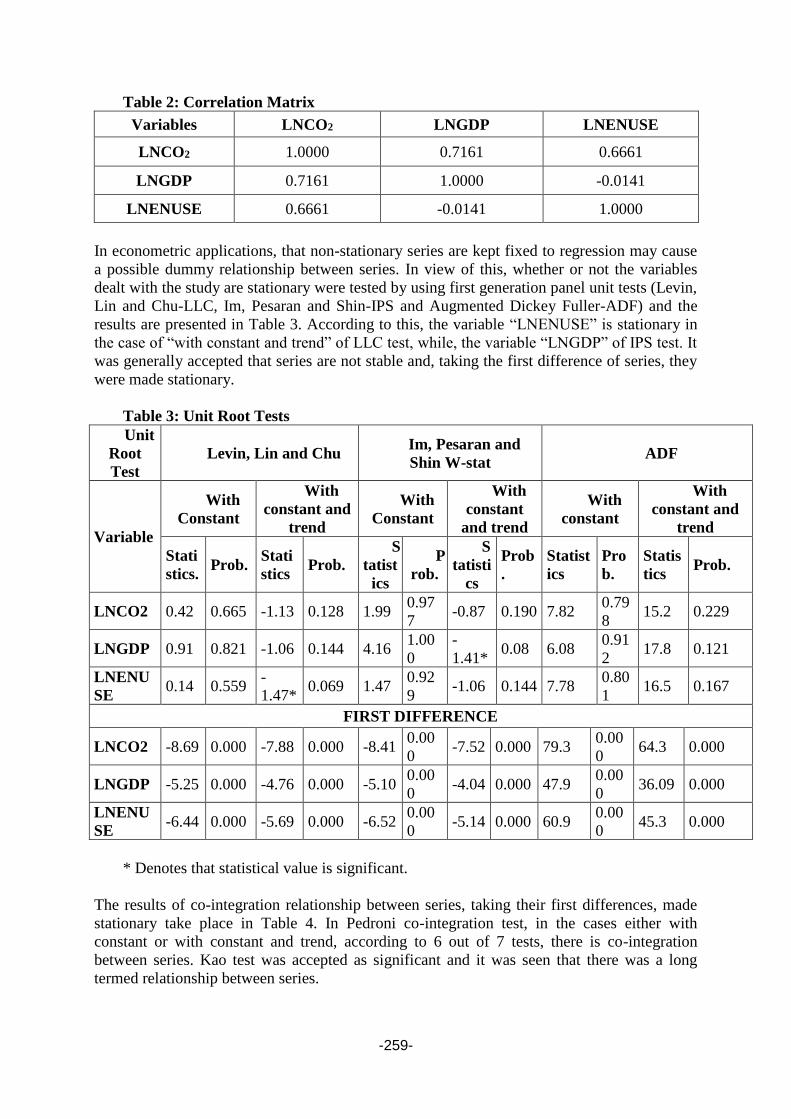
http://www.eia.gov/cfapps/ipdbproject/iedindex3.cfm?tid=90&pid=44&aid=8

-259-

Table 2: Correlation Matrix

Variables LNCO2 LNGDP LNENUSE

LNCO2 1.0000 0.7161 0.6661

LNGDP 0.7161 1.0000 -0.0141

LNENUSE 0.6661 -0.0141 1.0000

In econometric applications, that non-stationary series are kept fixed to regression may cause

a possible dummy relationship between series. In view of this, whether or not the variables

dealt with the study are stationary were tested by using first generation panel unit tests (Levin,

Lin and Chu-LLC, Im, Pesaran and Shin-IPS and Augmented Dickey Fuller-ADF) and the

results are presented in Table 3. According to this, the variable “LNENUSE” is stationary in

the case of “with constant and trend” of LLC test, while, the variable “LNGDP” of IPS test. It

was generally accepted that series are not stable and, taking the first difference of series, they

were made stationary.

Table 3: Unit Root Tests

Unit

Root

Test

Levin, Lin and Chu Im, Pesaran and

Shin W-stat ADF

Variable

With

Constant

With

constant and

trend

With

Constant

With

constant

and trend

With

constant

With

constant and

trend

Stati

stics. Prob.

Stati

stics Prob.

S

tatist

ics

P

rob.

S

tatisti

cs

Prob

.

Statist

ics

Pro

b.

Statis

tics Prob.

LNCO2 0.42 0.665 -1.13 0.128 1.99 0.97

7 -0.87 0.190 7.82

0.79

8 15.2 0.229

LNGDP 0.91 0.821 -1.06 0.144 4.16 1.00

0

-

1.41* 0.08 6.08

0.91

2 17.8 0.121

LNENU

SE 0.14 0.559

-

1.47* 0.069 1.47

0.92

9 -1.06 0.144 7.78

0.80

1 16.5 0.167

FIRST DIFFERENCE

LNCO2 -8.69 0.000 -7.88 0.000 -8.41 0.00

0 -7.52 0.000 79.3

0.00

0 64.3 0.000

LNGDP -5.25 0.000 -4.76 0.000 -5.10 0.00

0 -4.04 0.000 47.9

0.00

0 36.09 0.000

LNENU

SE -6.44 0.000 -5.69 0.000 -6.52

0.00

0 -5.14 0.000 60.9

0.00

0 45.3 0.000

* Denotes that statistical value is significant.

The results of co-integration relationship between series, taking their first differences, made

stationary take place in Table 4. In Pedroni co-integration test, in the cases either with

constant or with constant and trend, according to 6 out of 7 tests, there is co-integration

between series. Kao test was accepted as significant and it was seen that there was a long

termed relationship between series.

-260-

Table 4: Panel Co-Integration (Pedroni) and Kao Tests

With Constant With Constant and Trend

Statistics Statistics Probability Statistics Statistics

Panel v-Statistics -0.612774* 0.7300 -2.259886* 0.9881

Panel rho- Statistics -5.255291 0.0000 -3.410989 0.0003

Panel PP- Statistics -14.09343 0.0000 -20.28475 0.0000

Panel ADF- Statistics -9.605750 0.0000 -11.21622 0.0000

Grouprho- Statistics -4.757641 0.0000 -2.893261 0.0019

Group PP- Statistics -16.65782 0.0000 -23.34123 0.0000

Group ADF- Statistics -10.82805 0.0000 -10.70482 0.0000

Kao Test

t-statistics Probability

-5.8464 0.0000

*Coefficient is insignificant.

After identifying that there was a long termed relationships between series, the direction and

coefficients of short and long termed relationships between variables can be estimated by

means of the predictors PMGE and MGE. In this direction, panel vector error correction

model can be formulated as follows:

In the model, denotes error correction parameter; , coefficients of lagged dependent

variable (scalars); , coefficient vectors; index i, the number of country; r, time; q,

optimal lagging length; and , the term error. That error correction factor is negative valued

and statistically significant reveals that short termed deviations between co-integrated series

will disappear in the long period and that series will reach equilibrium in the long period.

The relationship between LNCO2 and LNGDP and LNENUSE was estimated by the

estimators PMGE and MGE and, in order to identify which of these predictors reveals better

results, Hausman Test, which test long termed homogeneity, was applied. The findings

obtained are presented in Table 5. Chi square value of Hausman test is not significant and H0

hypothesis not rejected. That is, the PMGE produces correct results and long term parameters

are homogenous. On the other hand, since error correction parameter is less zero, it is

significant; hence, there is a long termed relationship between variables.

Table 5: The Results of PMGE and Hausman Tests

D. CO2 Coefficient Standard

Error z statistics

P > | z

|

%95 Confidence

range

Ec

LNGDP 1.129366 .0121619 92.86*** 0.000 1.105529

1.15320

3

Ec 1.217519 .0303643 40.10*** 0.000 1.158006 1.27703

-261-

LNENUSE 2

SR

Ec -.5891287 .1463 -4.03*** 0.000 -.8758713

-

.302386

LNGDP

D1. .5472602 .264673 2.07** 0.039 .0285107 1.06601

LNENUSE

D1. .3380834 .199398 1.70* 0.090 -.0527296

.728896

3

Constant -17.83955 4.433839 -4.02*** 0.000 -26.52971

-

9.14938

4

HAUSMAN TEST

Hausman Test: Prob> = 0.3994 Log Probability: 297.3125 Number of

Observation (n): 124

*** p<0.01, ** p<0.05, * p<0.1

Error correction parameters also shows the speed of short term deviations, resulted from

not being stationary of series, to reach equilibrium in the next period. According to this, about

59% of unbalances forming in a period will get better in the next period and it will be

provided it to approach to the long term equilibrium. Either short (0.34 and 0.35, respectively)

and long term (1.22 and 1.23) parameters of the variables LNENUSE and LNGDP are

significant. It can be expressed that the findings overlap with economic expectations. In the

long term, increase of 1% in energy use and GDP increases CO2 in the rates of about 1.22%

and 1.23%, respectively. In the short term, these coefficients range as 0.34% and 0.55%.

In terms of unit effects, as seen in Table 6, in the country group considered in the long

term, the coefficients belonging to error correction parameters of Russia, India, China, South

Africa, and Turkey were found significant. In view of this, in the mentioned countries,

between CO2 remission, energy use, and GDP, there is a long termed relationship.

Table 6: Long Term Confidents Belonging to Countries a

Countrie

s D.lnco2 Coefficient

Standa

rd

Error

Z

Statistics

Probabili

ty

[95% confidence

interval]

__eca

lnGDP 1.129366 .012161

9

92.86*** 0.000 1.10552

9

1.15320

3

lnENUS

E

1.217519 .030364

3

40.10*** 0.000 1.15800

6

1.27703

2

BRAZIL

__ec -.0560133 .138131

3

-0.41 0.685 -

.3267458

.2147192

lnGDP

D1.

1.32212 .330249

8

4.00*** 0.000 .674842

7

1.96939

8

lnENUS

E D1.

.6889029 .28696 2.40** 0.016 .1264716 1.251334

_cons -1.728596 4.23676

7

-0.41*** 0.683 -

10.03251

6.575316

RUSSIA

__ec -.7240128 .219581 -3.30*** 0.001 -

1.154384

-.293642

lnGDP .2435448 .285105 0.85 0.393 - .8023413

-262-

D1. 5 .3152517

lnENUS

E D1.

.1662928 .349895 0.48** 0.635 -

.5194888

.8520743

_cons -21.9283 6.64541

7

-3.30*** 0.001 -

34.95308

-8.90352

INDIA

__ec -.4572247 .141964

6

-3.22*** 0.001 -

.7354703

-.1789791

lnGDP

D1.

1.431257

.38665

64

3.70*** 0.000 .6734245 2.18909

lnENUS

E D1

1.122688 .442928

5

2.53** 0.011 .2545641 1.990812

_cons -13.75996 4.28150

9

-3.21*** 0.001 -

22.15157

-5.36836

CHINA

__ec -1.139569 .135202

7

-8.43*** 0.000 -

1.404561

-.8745764

lnGDP

D1.

.0753296 .162186

9

0.46 0.642 -

.242551

.393210

1

lnENUS

E D1.

-.2597436 .163388

8

-1.59 0.112 -

.5799799

.0604926

_cons -34.53727

3.9522

17

-8.74*** 0.000 -

42.28347

-26.79106

SOUTH

AFRICA

__ec -.4812129 .208127

7

-2.31** 0.021 -

.8891357

-.0732901

lnGDP

D1.

.019917 .359097

8

0.06 0.956 -

.6839017

.7237358

lnENUS

E D1.

.1431009

.2428223

0.59 0.556 -.332822 .6190238

_cons -14.55388

6.2933

02

-2.31** 0.021 -

26.88852

-2.219232

TURKE

Y

__ec -.6767393 .211995

2

-3.19*** 0.001 -

1.092242

-.2612363

lnGDP

D1.

.1913922 284430

3

0.67 0.501 -.366081 .7488654

lnENUS

E D1.

.1672592 .340493

9

0.49 0.623 -

.5000966

.834615

_cons -20.52929 6.42714

6

-3.19*** 0.001 -

33.12627

-7.932317

a : Represents error correction parameter . *** p<0.01, ** p<0.05, * p<0.1

In the study, it was researched whether or not there was a causality relationships

between series. In this scope, conducting Granger and Dumitrescu Hurlin panel causality

tests, the results are presented in Table 7. According to the results of Granger causality test, in

the country group forming sample, there are the bidirectional relationship between energy use

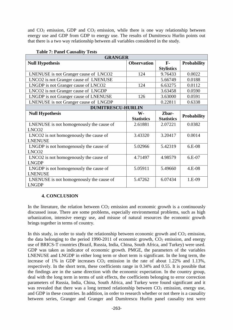
-263-

and CO2 emission, GDP and CO2 emission, while there is one way relationship between

energy use and GDP from GDP to energy use. The results of Dumitrescu Hurlin points out

that there is a two way relationship between all variables considered in the study.

Table 7: Panel Causality Tests

GRANGER

Null Hypothesis Observation F-

Stylistics

Probability

LNENUSE is not Granger cause of LNCO2 124 9.76433 0.0022

LNCO2 is not Granger cause of LNENUSE 5.66749 0.0188

LNGDP is not Granger cause of LNCO2 124 6.63275 0.0112

LNCO2 is not Granger cause of LNGDP 3.63458 0.0590

LNGDP is not Granger cause of LNENUSE 126 3.63000 0.0591

LNENUSE is not Granger cause of LNGDP 0.22811 0.6338

DUMITRESCU-HURLIN

Null Hypothesis W-

Statistics

Zbar-

Statistics Probability

LNENUSE is not homogenously the cause of

LNCO2

2.61881 2.07221 0.0382

LNCO2 is not homogenously the cause of

LNENUSE

3.43320 3.20417 0.0014

LNGDP is not homogenously the cause of

LNCO2

5.02966 5.42319 6.E-08

LNCO2 is not homogenously the cause of

LNGDP

4.71497 4.98579 6.E-07

LNGDP is not homogenously the cause of

LNENUSE

5.05911 5.49660 4.E-08

LNENUSE is not homogenously the cause of

LNGDP

5.47262 6.07434 1.E-09

4. CONCLUSION

In the literature, the relation between CO2 emission and economic growth is a continuously

discussed issue. There are some problems, especially environmental problems, such as high

urbanization, intensive energy use, and misuse of natural resources the economic growth

brings together in terms of country.

In this study, in order to study the relationship between economic growth and CO2 emission,

the data belonging to the period 1990-2011 of economic growth, CO2 emission, and energy

use of BRICS-T countries (Brazil, Russia, India, China, South Africa, and Turkey) were used.

GDP was taken as indicator of economic growth. PMGE, the parameters of the variables

LNENUSE and LNGDP in either long term or short term is significant. In the long term, the

increase of 1% in GDP increases CO2 emission in the rate of about 1.22% and 1.13%,

respectively. In the short term, these coefficients range in 0.34% and 0.55. It is possible that

the findings are in the same direction with the economic expectation. In the country group,

deal with the long term in terms of unit effects, the coefficients belonging to error correction

parameters of Russia, India, China, South Africa, and Turkey were found significant and it

was revealed that there was a long termed relationship between CO2 emission, energy use,

and GDP in these countries. In addition, in order to research whether or not there is a causality

between series, Granger and Granger and Dumitrescu Hurlin panel causality test were

-264-

conducted. According to the results of Granger causality tests, there was a two way

relationship between energy use and CO2 emission and between GDP and CO2 emission,

while there was a one way relationship between GDP and energy from GDP to energy use.

The results of Dumitrescu Hurlin points out that there is a two way relationship between all

variables used in the study.

REFERENCES

1. Arı, Ayşe & Zeren, Fatma (2011). CO2 Emisyonu ve Ekonomik Büyüme: Panel Veri

Analizi. Celal Bayar Üniversitesi İktisadi ve İdari Bilimler Fakültesi Yönetim ve Ekonomi

Dergisi, 18 (2), 37-47.

2. Aytun, Cengiz (2014). Gelişen Ekonomilerde Karbondioksit Emisyonu, Ekonomik Büyüme

ve Eğitim Arasındaki İlişki: Panel Veri Analizi.

http://www.jasstudies.com/Makaleler/1669013076_22-

%20Dr.%20Cengiz%20AYTUN.pdf, 14.06.2015.

3. Başar, Selim & Temurlenk, M. Sinan (2007). Çevreye Uyarlanmış Kuznets Eğrisi:

Türkiye Üzerine Bir Uygulama. Atatürk Üniversitesi İktisadi ve İdari Bilimler Dergisi, 21

(1), 1-12.

4. Begum, Rawshan Ara et al. (2015). CO2 Emissions, Energy Consumption, Economic and

Population Growth in Malaysia. Renewable and Sustainable Energy Reviews, 41, 594-

601.

5. Bruvoll, Annegrete & Medin, Hege (2003). Factors Behind The Environmental Kuznets

Curve A Decomposition of The Changes in Air Pollution. Environmental and Resource

Economics, 24 (1), 27–48.

6. Dam, Mehmet Metin, Karakaya, Etem & Bulut, Şahin (2013). Çevresel Kuznets Eğrisi ve

Türkiye: Ampirik Bir Analiz.

http://birimler.dpu.edu.tr/app/views/panel/ckfinder/userfiles/17/files/DERG_/EY___ZEL_

SAYI/7.pdf, 14.06.2015.

7. Gao, Jing & Zhang, Lei (2014). Electricity Consumption–Economic Growth–CO2

Emissions Nexus in Sub‐Saharan Africa: Evidence from Panel Cointegration. African

Development Review, 26 (2), 359-371.

8. Grossman, Gene M. & Krueger, Alan B. (1991). Environmental Impacts of A North

American Free Trade Agreement. http://www.nber.org/papers/w3914.pdf, 02.05.2015.

9. Grossman, Gene M. & Krueger, Alan B. (1995). Economic Growth and the Environment.

The Quarterly Journal of Economics, 110 (2), 353-377.

10. Joo, Young-Jong, Kim, Chang Seob & Yoo, Seung-Hoon (2015). Energy Consumption,

CO2 Emission, and Economic Growth: Evidence from Chile. International Journal of

Green Energy, 12 (5), 543-550.

11. Kuznets, Simon (1955). Economic Growth and Income Inequality. The American

Economic Review, 45 (1), 1-28.

12. Lee, Jung Wan & Brahmasrene, Tantatape (2014). ICT, CO2 Emissions and Economic

Growth: Evidence from a Panel of ASEAN. Global Economic Review, 43 (2), 93-109.

13. Magazzino, Cosimo (2015). Economic Growth, CO2 Emissions and Energy Use in Israel.

International Journal of Sustainable Development & World Ecology, 22 (1), 89-97.

http://www.jasstudies.com/Makaleler/1669013076_22-%20Dr.%20Cengiz%20AYTUN.pdf

http://www.jasstudies.com/Makaleler/1669013076_22-%20Dr.%20Cengiz%20AYTUN.pdf

http://birimler.dpu.edu.tr/app/views/panel/ckfinder/userfiles/17/files/DERG_/EY___ZEL_SAYI/7.pdf

http://birimler.dpu.edu.tr/app/views/panel/ckfinder/userfiles/17/files/DERG_/EY___ZEL_SAYI/7.pdf

http://www.nber.org/papers/w3914.pdf

-265-

14. Nautz, Dietere & Rondorf, Ulrike (2010). The (In)stability of Money Demand in the Euro

Area: Lessons from a Cross Country Analysis. http://edoc.hu-berlin.de/series/sfb-649-

papers/2010-23/PDF/23.pdf, 02.06.2015.

15. Omri, Anis (2013). CO2 Emissions, Energy Consumption and Economic Growth Nexus in

MENA Countries: Evidence From Simultaneous Equations Models. Energy Economics,

40, 657-664.

16. Omri, Anis, Nguyen, Duc Khuong & Rault, Christophe (2014). Causal (Dynamic

Simultaneous-Equation Models. Economic Modelling, 42, 382-389.

17. Pesaran, M. Hashem, Shin, Yongcheol ve Smith, Ron P. (1999). Pooled Mean Group

Estimation of Dynamic Heterogeneous Panels. Journal of the American Statistical

Association, 94 (446), 621-634.

18. Saatçi, Mustafa & Dumrul, Yasemin (2011). Çevre Kirliliği ve Ekonomik Büyüme

İlişkisi: Çevresel Kuznets Eğrisinin Türk Ekonomisi İçin Yapısal Kırılmalı Eş-

Bütünleşme Yöntemiyle Tahmini. Erciyes Üniversitesi İktisadi ve İdari Bilimler Fakültesi

Dergisi, (37), 65-86.

19. U.S. Energy Information Administration. International Energy Statistics.

http://www.eia.gov/cfapps/ipdbproject/iedindex3.cfm?tid=90&pid=44&aid=8,

01.06.2015.

20. World Bank. World Development Indicators. http://databank.worldbank.org,

01.06.2015.

21. Yenigün, Ethem (2011). Sürdürülebilirlik Kavramının Uluslararası Gündeme Gelmesi.

http://yesilekonomi.com/kose-yazilari/ethem-yenigun/surdurulebilirlik-kavraminin-

uluslararasi-gundeme-gelmesi, 02.06.2015.

http://www.eia.gov/cfapps/ipdbproject/iedindex3.cfm?tid=90&pid=44&aid=8

http://databank.worldbank.org/

http://yesilekonomi.com/kose-yazilari/ethem-yenigun/surdurulebilirlik-kavraminin-uluslararasi-gundeme-gelmesi

http://yesilekonomi.com/kose-yazilari/ethem-yenigun/surdurulebilirlik-kavraminin-uluslararasi-gundeme-gelmesi

-266-

THE IMPACT OF BILATERAL INVESTMENT TREATIES (BITS) AS A

POLITICAL RISK MITIGATOR ON ATTRACTING FOREIGN DIRECT

INVESTMENT (FDI)

Zhiyar Ismael


Abstract

This study tries to explore the role of BITS as a type of International Investment Agreements

(IIAS) on protecting cross- border investment and global operation businesses. The study asks

whether or not BITS mitigate political risks among countries solicitous of this type of

agreements and whether they stimulate FDI to host countries. Several efforts have presented

in this field of study through examining many variables that affect the relationship between

BITS and FDI. This study reveals about the different results have extracted in this field of

literature.

Keywords: Risk Management, International Investment Agreements (IIAs), Foreign Direct

Investment (FDI)

Introduction

In 21st century world trade, the policies and rules underpinning investment and trade which

consider barriers to entry have become the rules of international trade in an effective way

(Global Agenda Council on Global Trade and FDI, 2013). The regulatory and legal

environment of countries have a great role in shaping the trade and investment decisions.

Many nations have embraced the amount of liberalization stated in Regional Trade

Agreements (RTAs) and International Investment Agreements (IIAs), while others found it

contradicted with their main Foreign Direct Investment (FDI) rules and conditions and

adopted protectionist measures in their Bilateral Investment Treaties (BITs) against it, for

example, Japan is one of the nations that have strict barriers to foreign entry.

Multinational enterprises around the world face different types of risks especially in

nowadays dynamic and unstable environment, these risks may be outside the control of

multinationals caused by fluctuations in economic variables called Macroeconomic Risks.

Another type of risks facing the majority of firms operating across national boundaries called

Political Risks or Policy Risks which arise from policy reversal or more generally from policy

actions of host governments, this type of risks is the core subject of this review study. The

third type of risks is Competitive Risks arising from the unpredictable reactions of

competitors (competitors’ responses). The last type of risks called Resource Risks arising

from the adoption of strategies that require resources in which organizations are unable to

acquire it (Ghoshal, 1987).

The literature of international trade and political science and economics provide conflicting

results for the claimed relationship and connection between BITs and FDI, many moderating

and mediation factors such as political environment of host countries, the structure of political

institutions in host countries, equitable domestic institutional systems, population, location,

GDP, levels of domestic investment and many other antecedents have taken in consideration

to better determine the magnitude of the conditional relationship between BITs and FDI

(Yackee, 2007; Tobin and Ackerman, 2011).

-267-

Political Risks’ Meaning

Although political risks of international business received wide academic interest, it still a

new term and has not limited meaning, because it has been described in different studies

based on different implications of its unwanted consequences. But, political risks most

commonly defined as government (usually host country) interference with business operations

(Kobrin, 1979), another representative definition of political risks presented by Waston and

Sorge, 1972 states that political risks arise from national governments’ actions to prevent

business (foreign investment) transactions, reverse policies in a way that contradict with their

agreements with foreign investors, or confiscate (seizing) foreign investors properties partially

or totally specially through coups in which the new in power political force may place a

radical socialist system and expropriate foreign investors assets. Another cluster of authors

defines the term political risk as environmental factors such as political instability or direct

violence represented in constrains on foreign investment operations such as expropriation and

confiscation, discriminatory taxation, unequitable treatment, and the like. In accordance to all

the presented perspectives of political risk definition, we can define it as a combination of

risks that are under the control of governments such as policy changing represented in

changing exchange and interest rates, prices, import restrictions, expropriation, domestic

arbitration, and risks that are unpredictable and out of the control of governments such as

revolutions and political changes, labor strikes, and terrorism, that harm the normal

circumstances of foreign investors to continue their business, attain profits, or maintain their

market share in host countries.

The Political Risks of Global Business

The economic policies of nations are highly related with their political institutions in which

the political systems can enhance the stability of countries’ economic policies and let foreign

investors to have perceptions about how the future economic and political conditions will

become in the host countries, these perceptions determine investors decisions because

political institutions’ ability to provide credible commitment to economic policies in host

countries is the most important element affecting foreign investors decisions. Accordingly,

many nations are competing to provide better and better “market- friendly” policies for

multinational enterprises (MNEs) to attract high levels of FDI flows.

The majority of studies presented in the literature of international investment, political risks of

global business, and foreign direct investment illustrate that MNEs prefer to invest in

countries with less policy risks (Holburn and Zelner, 2010).

After the economic crisis of 2008, many affected countries signed agreements with the

International Monetary Fund (IMF) in an attempt to attain the required capital for recovering

their financial problems. IMF conditions tie the lent loans to the availability of specific

economic policies such as “market friendly” policies and policy stability. IMF conditionality

expected to have a positive impact on the flows of FDI to countries under IMF program, but

the opposite usually happens because IMF conditions caused protests and violence that lead to

political and social instability in low and middle- income countries. As a result, we can say

that the loans governments receive it from IMF may increase policy stability in these

countries but, in the other side, it rises violence and political instability which lead

multinational enterprises to step back from investing in these countries.

-268-

Foreign Investors’ Decisions and Political Risks

Understanding different aspects of political risks and integrating it to investment decision-

making consider a fundamental expertise for foreign investors that somewhat protect their

assets and efforts to go waste. Foreign investors, through the process of decision making,

confront big challenges represent in their capabilities to associate the probability of occurring

a specific event (risk) with its outcomes. This logical judgment may be successful in case of

systemic domestic risks which relate to the domestic institutional system of host countries and

could be predicted from reviewing the subsequent behavior of host country or analyzing the

statistics of its past experience. But in the case of unpredictable events, decision-makers

neither predict the probability of occurring these risks nor their possible outcomes such as

wars, terrorism, revolutions.

Uncertainty is usually subjective which realizing the likelihood of occurring certain events in

such circumstances need a combination of many non-cognitive skills, information, and data

that form perceptions enable foreign investors to slightly predict occurring some risks. Many

empirical studies in the literature of international trade examine different environmental

factors particularly political instability and market size which these two factors had the most

significant impact on FDI flows. A cross-sectional study done over 62 countries by Kobrin in

1976 analyzed the impact of seven economic, social, and political factors on US

manufacturing FDI flows. He concluded that the overall impact of all studied environmental

factors on FDI was 64%, whilst market size and the prior exports of US took the biggest

portion of this impact and record high significance over political instability. This result might

not be the same if this study apply in one of the developing countries, because US as a

developed country provide high levels of protection for foreign investors in their legislations

and policies, which lead investors to concentrate on their environmental analysis more on

market size and other factors helping them to maximize their market share and profits over

than political issues (Kobrin, 1979) Kobrin, 1978 found that interstate conflicts have a

significant impact on FDI practically when these conflicts estimate to have unfavorable

outcomes for foreign investors such as changing government policies (Korbin, 1978).

Changing leadership either formally through election or through coups and revolutions

considers one of the most perilous political risks facing foreign investment particularly in

developing countries, this risk usually arise from host countries and threaten multinational

enterprises investing in these countries as well as, harming FDI flows to such countries. But

we might see the occurrence of this risk from home countries, this case is obvious now after

Donald Trump take over US presidency in which he repeatedly promise US people in his

debates to break the international investment treaties between US and China to draw back the

American- base technological multinational enterprises investing in China. This leadership

change estimate to affect FDI inflows and outflows with China because the importance of

China’s outflow with US which ranked at third place in both 2014 and 2015, the total

investment of Chinese multinationals in US records $15.7 billion in 2015 a 30 % increase

from 2014 (Hanemann and Gao, 2016), most of this investment was through 103 merges and

acquisitions (M&A) deals worth $14 billion, in the other hand this leadership change may also

affect the American multinationals investing in china such as Apple co. in which the price of

its new generations of iphone estimate to increase to more than $1300 if it start to produce in

US.

-269-

The Structure of Political Institutions and Political Risks

The literature of international investment devoted an exaggerated attention to the fiscal

competition among countries to attract FDI by lowering taxation levels (Jensen, 2006), while

the impact of political institution structure on FDI remain under-development in the literature

and an obvious contrast can be found about the impact of democratic and authoritarian

political institutions to attract FDI.

Most scholars interested in studying the impact of various political institutions on FDI flows

declare an availability of positive linkage between domestic political institution and high

levels of FDI, this derivation came out from the reality of associating balanced movements

and policy changing with democratic systems and their role in activating policy stability.

Policy stability encourages multinational corporations and allow them to plan for their

investment, analyze the macroeconomic environment more accurately, and make investment

decisions according to the predicted information and forecasted data (Jensen, 2003, 2006).

Some efforts in the literature devoted toward the study of multinationals preferences to invest

in dictatorships, but this area of study has not concluded serious results and remain under

development. The main idea that these studies based on is the desire of some multinational

enterprises to bargain with authoritarians because of the low levels of leader turnover in these

countries which provide policy stability, as well as arranging opportunities for foreign

investors even if is not the favor of their countries’ domestic growth and development but

usually lent personal interests to authoritarian leaders whom have substantial influence over

governments.

Jensen 2006 declared that multinational investors prefer to invest in democratic nations over

authoritarians for three basic reasons:

1- Democratic nations are more transparence in their legislations and affairs, and

offer clear information. This transparency allow multinational firms to invest

confidently in democratic nations over than authoritarian regimes.

2- The author clarifies the role of representation in attracting FDI in democratic

countries. Representation means that foreign investment countries can influence

democratic host countries through lobbying their preferred conditions, while it seems

not existed in authoritarian countries. In this case, democratic nations try to provide

favorable legislations to foreign investment in balance with their domestic.

3- Credibility is the third mechanism offered in Jensen’s 2006 study, credibility

means the ability of political institutions of host countries to deal with rises political

risks in favor of the multinational enterprises. Democratic nations consider credible

systems because the political institutions of these countries create incentives for their

governments to provide political stability that attract FDI balanced with their domestic

investment. Democratic nations prove their credibility through the subsequent

commitment to signed agreements in these countries (Allee and Peinhardt, 2011).

The quality of political and diplomatic relations between home and host countries is the most

important factor affecting foreign investors decisions, the political risks that related to each

pair of these countries and interstate political relations called Idiosyncratic Risks, while that

related to domestic institutional system which are more common to investors called Systemic

Domestic Risks. A study performed in 2007 by Desbordes and Vicard analyzed data collected

from 30 OECD countries and 62 non- OECD countries found that diplomatic relations

significantly affect FDI flows, but this relationship can be mitigated by the entry of BITs. It

-270-

means that BITs have an important indirect impact on FDI flows over the impact of interstate

political relations (Desbordes and Vicard, 2007; Neumayer and Spess, 2005).

As the political and legal environment of many developing and transition economies are weak

and unstable, investors desiring to invest in these countries seek to have tailored alternative

rules that protect their property rights and reduce the systemic domestic and idiosyncratic

risks facing them (Tobin and Ackerman, 2003), BITs consider one of the most effective

elements of securing the legal phenomenon of foreign investment , resolving disputes between

the host and home countries through the International Center for the Settlement of

International Disputes (ICSID), facilitating the access of financial resources (UNCTAD,

1998), and fulfilling policy credibility by transition and developing countries.

BITs and FDI

Singing agreements between foreign investors and host countries are complex processes and

are not free of mutual criticism. Multinational enterprises and host countries both suffer from

a little trust of the rights and obligations reliability that have been agreed on previously (Tobin

and Ackerman, 2003) which usually caused by the deterioration of the diplomatic relations

between home and host countries (Desbordes & Vicard, 2007). No one can ignore the

existence of such troubles among the contracting parties, as each side seek assurances and

interest that guarantee achieving their goals that should balance with the goals of the side.

BITs are general frameworks between two (host and home) countries imply a band of rules

that ensure Foreign investment Protection. These agreements are usually set by host countries

that facilitate the negotiations of FDI, and have relatively similar provision unless some

differences in the way of provided protection, capital flow, repatriation of profits, the

equivalent treatment of domestic and foreign firms, etc., BITs also differ from each other in

excluding investment in particular sectors or areas such as telecommunication industry.

Although BITs have unlimited interest for all countries interested in attracting FDI, some of

these countries might not be cautions enough about BITs negative consequences if it has not

been prepared carefully in the way that guarantee balanced interests for the host and home

countries, but instead it may harm the national industry of host countries and lead them to loss

sovereignty over their domestic investment disputes. Counties fear of losing the sovereignty

over their internal activities and policies through the restrictions that many BITs drafts include

it, lead many host countries to refuse signing these BITs, the US BIT with Honduras in the

early 1980s was exact example on this case in which Honduras refused signing a $ 5 billion

investment BIT because it included clauses violated to Honduran legislation.

In general, US and several European BITs try to decrease the greediness of many foreign

investors caused by host countries’ race to the bottom (RTB) attract them, as well as the

leverage of host countries over foreign investors through prohibiting investment performance

requirements that usually affecting the investment decisions of multinationals int favor of host

nations. Repatriation of profits is an example of investments performance requirement in

which some treaties’ clauses enable host countries in economic emergency times to delay

foreign investors’ repatriation of profits. Despite the advantages and disadvantages appeared

from signing BIT agreements between host and home countries, but it still consider a very

powerful mechanism of internationalizing the commercial law as a way of reducing the

disputes between contracting sides.

-271-

The history of signing first BITs goes back to the end of 1950s in which Germany took the

lead in this area when in concluded an agreement with Pakistan in 1959 after a massive suffer

from losing approximately all of its foreign investment after world war II (Salacuse &

Sulivan, 2005), while some authors trace their roots to the friendship, commerce, and

navigation (FCN) treaties that US concluded the over countries as a tool of improving its

foreign relations. Although the opinions of scholars vary about the availability of significant

relationship between BITs and FDI, the number of signed BITs is increasing dramatically

year after another, this growth in BITs numbers prove the importance of these agreements, the

number of formed BITs were 75 by the end 1960s, then they rose to 176 and 389 by the end

of the 1970s and 1980s respectively. The most rapid growth of BITs signed worldwide were

between 1990s and 2002 which arrived 2181 BITs, and the vast majority of them were

concluded between developed and developing countries (Neumayer & Spess, 2005) at the aim

of providing certain standards of treatment or better treatment for the foreign investors over

the domestic investors.

The main purpose of concluding BITs particularly in developing countries is guaranteeing

certain standards of treatment and creating incentives for host countries government to

complicate policy reversal and maximize policy stability for foreign investors. These

provisions are fundamental factors to bypass some problems facing developing countries such

as “hold-up” or “dynamic inconsistency”, this problem arises in the host countries that have

promised foreign investors an equitable treatment in their domestic legal rules to promote the,

but once the foreign investors established and have sunk significant capital in operation, the

host country begin to expropriate their assets through changing the regulations, pricing,

taxing, and the like (Coleman, Davidson, low & Pryce, 2012), because of that, foreign

investors cannot trust the host countries domestics legal rules and prefer to attain protection

through international legal binds and arbitration represented in BITs.

As a result, we can say that BITs are important elements for protecting foreign investment

that currently have not much alternatives unless few agreements of regional free trade such as

North American Free Trade Agreement (NAFTA) and World Trade Organization’s (WTO)

Agreement.

BITs usually conclude between developed and developing countries, it could be seen formed

between two developing countries or two developed countries as well, such as BITs between

Egypt and Morocco, and between United States and Japan (Salacuse et al, 2005).

Establishing international business or investment in developing countries usually needs

concluding agreements such as BITs that guarantee certain levels of protection for foreign

investors, because the political and economic policies in these countries are unstable and

usually controlled by governments’ sovereignty, but the case of Brazil is exception to this

estimation. Although Brazil is one of the developing countries (Poulsen, 2010) that bogged

down by an ongoing instability in its political and economic situation, and nowadays is

witnessing a leadership transition which Brazilian people forced president Dilma Rousseff to

step down and allow her vice president to take over the position as interim president

(Flannery, 2016), it attract large levels of FDI without any BITs. The absence of BITs did not

impede the plentiful flow of foreign investment to Brazil. Many studies such as Unite Nations

Conference on Trade and Development (UNCTAD) return the reason behind this much

investment to Brazil to the quality of its domestics policies and regulation that provide

standards favorable to foreign investors.

-272-

Reviewing different perspectives of international trade literature induce us to consider many

other environmental factors in consideration rather than policy stability as Brazil has a

population more than the population of other South American countries combined (Infante,

2015), this lead us to think that market size and population have significant impact on foreign

investors decisions to invest in certain location.

FDI in 21st Century

FDI consider a powerful and major form of international capital transformation among

nations and enhance their economic growth prosperity and development through creating

jobs, promoting knowledge, exchanging information and expertise, transferring technology,

increasing the productivity in different sectors, modernizing the domestic industry and

increasing employment levels.

FDI witnessed a dramatic increase at the end of 20th century and more accurately between

1980 and 1990 which it has tripled. FDI as a form of transforming the international capital has

become the most efficient entry strategy to international business (IB) over the licensing,

franchising, turnkey operations, etc.(Froot, 1993).

The advancement in FDI that the world witness it nowadays is a consequence of the first step

taken by US to move oversea post world war II. At that time, US firms were advanced in

technology that let them access foreign markets even to achieve competitive advantages as a

first or to obstruct competitors’ access, then it dramatically turned from a home for many

multinational firms to a host for foreign multinationals specially European, Canadian, and

Japanese-based multinational enterprises which the person sometimes can feel that, these

foreign multinationals have a control over certain assets in US more than its based enterprises.

The 21st century’s FDI characterized by some different features than it was before. FDI’s

development, through the time, represented in many surges, each surge occurs in a certain

industry such as Japanese automobile production which let Japanese multinationals more

powerful as foreign investors and have a control over assets in the host countries. This surge

of industry lead US inflows and Japanese outflows to explore across all industries and become

larger and faster in growing. FDI also differs in the way of establishing the business. In the

past, multinationals were establishing investment in host countries from the base by

themselves, this way of business was a role and called greenfield investment which was $766

billion in 2015 (UNCTAD, 2016), but nowadays the majority of foreign investors are

establishing their investment in host countries through mergers and acquisitions (M&A)

which facilitate financing businesses.

In 2015, FDI flows reached highest level since the financial crisis of 2008 which became

$1.76 trillion a 38 % increase from 2014, however it still 10% less than it was in 2007 which

records highest levels of global FDI flow ever. A dramatic increase in cross-border M&A

from $432 billion in 2014 to $721 billion in 2015 was the fundamental factor behind this FDI

rebound. In accordance to the fragile global economy, weak aggregate demand, and falling

MNE profits, FDI expected to decrease in 2016, this expectation took place as it has been

illustrated in OECD, 2016 which the global FDI flows record $793 billion in the first half of

2016 a 5% decline compared to the second half of 2016 (OECD).

Conclusion

Many authors interested in economic literature illustrate that only successful governments are

changing their policies in accordance to the volatile political and economic circumstances in

-273-

an attempt to adjust their policies in the way that much with the international agreements such

as Bilateral Investment Treaties (BITs) and International Investment Agreements (IIAs). As a

result, we can say that the political institutions capable of providing credible commitments to

international investment policies and multinationals corporations will be more effective in

attracting FDI. Democratic institutions usually create incentives for their governments to

backtrack or renegotiate policies in a way that oppose the favor multinational enterprises,

these incentives usually consider key elements for achieving policy stability. Although policy

stability has been generally agreed on to have a positive impact on FDI flows, multinationals

look at it negatively when it relates to governments under IMF programs due to the political

and social effects caused by perceived loans such as violence and protests.

Many theoretical perspectives have been presented in the literature of international investment

such as “Ownership, Location, and Internalization (OLI) framework” presented by John

Dunning which studied these three factors as key elements affecting the decisions of

multinational firms to invest abroad or not. Many other theoretical models have been

developed by a number of scholars interested in multinationals decisions to invest abroad such

as “vertical” firms, “horizontal” firms, and the knowledge-capital model. Although these

theoretical frameworks and models are strong tools for understanding the multinationals

perceptions to invest abroad, they still shallow to answer the most critical question of foreign

investment: what features should host countries have to attract FDI? Because FDI remains a

totally firm-level decision which, as many other scholar thought, it affected more and more by

the political conditions of host countries, and the credibility of nation’s political institutions

that represented in the creative incentives for their governments make policy reversal more

difficult and maximize levels of policy stability. Also it is important to illustrate the

importance of the commitment and subsequent behavior of governments signing BITs on FDI

inflows. Governments that are more committed to comply BITs are more favorable to

multinational enterprises, BITs are very important international frameworks that guarantee

certain standards of treatment for multinationals especially in developing countries because

they can successfully overcome the political interference and regulatory sovereignty of host

countries to expropriate foreign investors, assets and reach the international arbitration.

References

1. Allee, T. & Peinhardt, C. (2011). “Contingent Credibility: The Impact of Investment Treaty

Violations on Foreign Direct Investment”, International Organization, 65 (3), 401- 432

2. Coleman, M., Davidson, s. k., Low, L. A., & Pryce, J. F. (2012). “Managing Political Risk

through Bilateral Investment Treaties”, [Web Page], Steptoe & Johnson, pp. 1- 5

3. Desbordes, R. &Vicard, V. (2007). “Foreign Direct Investment and Bilateral Investment

Treaties, an International Political Perspective”, [Working Paper], Pantheon- Sorbonne

University, Paris

4. Flannery, N. P. (2016). “Political Risk Outlook: How Will Brazil’s Economy Perform in

2016? Forbes Magazine

5. Franck, S. D. (2007). “Foreign Direct Investment, Investment Treaty Arbitration, and the

Role of Law”. Global Business & Development Law Journal, 19, 337- 373

6. Froot,K. A. (1993). “Introduction to Foreign Direct Investment”, United States, University of

Chicago Press, pp. 1-12

7. Ghoshal, S. (1987). “Global Strategy: An Organizing Framework”, Strategic Management

Journal, 8 (5), 425- 440

-274-

8. Global Agenda Council on Global Trade and FDI. (2013). “Foreign Direct Investment as a

Key Driver for Trade, Growth and Prosperity: The Case for a Multilateral Agreement on

Investment”, World Economic Forum, Geneva, Switzerland

9. Hanemann, T. & Gao, C. (2016). “Chinese FDI in the US: 2015 Recap”, [Web Site],

Rhodium Group

10. Holburn, G. L. F. & Zelner, B. A. (2010). “Political Capabilities, Policy Risk, and

International Investment Strategy: Evidence from the Global Electronic Power Generation

Industry, Strategic Management Journal, 31, 1290- 1315

11. Infante, A. (2015). “Doing Business with Brazil: 9 Differences from Brazil to US and other

Countries”, [Web Page], Street Smart Brazil

12. Jensen, N. M. (2003). “Democratic Governance and Multinational Corporations: Political

Regimes and Inflows of Foreign Direct Investment, International Organization, 57 (3), 587-

616

13. Jensen, N. M. (2006). “Nation- States and the Multinational Corporation: A Political

Economy of Foreign Direct Investment”, Princeton University Press

14. Kerner, A. & Lawrence, J. (2014). “What’s the Risk? Bilateral Investment Treaties, Political

Risk and Fixed Capital Accumulation”, British Journal of Political Science, 44 (1), 107- 121

15. Kobrin, S. J. (1978). “When Does Political Instability Result in Increased Investment Risk”,

The Columbia Journal of World Business, 13 (3), 113-122

16. Kobrin, S. J. (1979). “Political Risk: A Review and Reconsideration”, Journal of

International Business Studies, 10 (1), 67- 80

17. Neumayer, E. & Spess, L. (2005). “Do Bilateral Investment Treaties Increase Foreign Direct

Investment to Developing Countries? World Development, 33 (10), 1567- 1585

18. OECD (Organization for Economic Cooperation and Development). 2016. “FDI in Figures”

19. Poulsen, L. N. S. (2010). “The Importance Of BITs for Foreign Direct Investment and

Political Risk Insurance: Revisiting the Evidence”, New York, Oxford University Press, pp.

539- 574

20. Salacuse, J. W. & Sullivan, N. P. (2005). “Do BITs Really Work?: An Evaluation of Bilateral

Investment Treaties and Their Grand Bargain”, Harvard International Law Journal, 46 (1),

67-130

21. Tobin, J. & Ackerman,S. R. (2003). “Foreign Direct Investment and The Business

Environment in Developing Countries: The Impact of Bilateral Investment Treaties”,

[Working Paper]. The William Davidson Institute, No. 587

22. Tobin, J. L. & Ackerman, S. R. (2011). “When BITs Have Some Bite: The Political-

Economic Environment for Bilateral Investment Treaties”, The Review of International

Organizations, 6 (1), 1-32

23. UNCTAD (United Nations Conference on Trade and Development). (1998). “Bilateral

Investment Treaties in the Mid- 1990s. United Nations, New York and Geneva

24. UNCTAD (United Nations Conference on Trade and Development). (2016). “World

Investment Report 2016: Investor Nationality: Policy Challenges. United Nations, Geneva

25. Yackee, J. W. (2007). “Do BITs Really Work? Revisiting the Empirical Link between

Investment Treaties and Foreign Direct Investment”, [Research Paper], p.21

-275-

DO PRESS RELEASES PROVIDE NEW INFORMATION?

THE CASE OF BRITISH PETROLEUM‘S DEEPWATER HORIZON OIL SPILL

P. Sergius Koku

Florida Atlantic University/South Eastern European University

Eamil: [email protected]

Besnik Fatai

South Eastern European University, Macedonia

Fitim Deari


Izet Zeqiri


Abstract

This study evaluated the informational content of press releases and press conferences using

the British Petroleum’s 2010 Deepwater Horizon oil spill incident in which the company gave

52 press releases or press conferences in the 87-day event. The results show that, on average,

the market reacted negatively to the news releasing events (press releases or press

conferences). The average abnormal return was -0.67% with a t-value of -4.573 which was

significant at the -0.01 (two-tailed test). This suggests that new releasing events contained

new information which was perceived to be detrimental to the company. Contrary to the

popular myth that “there is no news as bad news”, there is indeed “bad news”, at least, in the

world of investment and corporate finance.

1. Introduction

The objective of this study is to evaluate the informational content of press releases or press

conferences using the British Petroleum’s 2010 Deepwater Horizon oil spill incident as a case

study. The study is important because a major event such as the Deepwater Horizon oil spill

has provided researchers in information economics an opportunity to rigorously analyze two

popular myths surrounding public information and communication – namely, (1) “there is no

news as bad news”, and (2) “corporate press releases and news conferences are no more than

a gimmick”. If the first assertion is true, then news on bad events should not negatively

impact companies, and in fact, on the contrary should help them. On the other hand, if the

second assertion is true, then corporate press releases and news conferences amount to no

more than a waste of resources – time and money.

The Deepwater Horizon Oil spill, which occurred in the Macondo Prospect in the Gulf of

Mexico in April, 2010, was the largest accidental oil spill in the United States (Robertson and

Clifford, 2010; Hoch, 2010; National Response Team, 2011). British Petroleum (BP) which

was primarily responsible for the environmental disaster tried without much success, through

initial press releases/news conferences, to implicate two other companies - Halliburtan and

Transocean as co-culprits (see Bates, 2010; Weber, Kunzelman and Cappiello, 2010).

BP, in an unprecedented move, held or released a total of 57 new conferences/ press releases

during the crisis that lasted for 87 days. Ostensibly, these events were to keep the public


-276-

informed, but critics dismissed them as “damage control” or “PR gimmick” given the

company’s inability to truthfully provide simple pertinent information such as the flow rate

during these news conferences or in press releases (see Robertson et al., 2010). The flow rate

was important because it gives the public an idea of how much damage was taking place and

what to expect.

To test the informational content of the press releases or press conferences held by British

Petroleum during the crisis, we used the event study technique (Samuelson, 1965; Fama,

1965, 1970), a well-received technique in finance, and data from the BBC (British

Broadcasting Communication) timeline chronicle.

2. Data

Several different news media covered events surrounding the spill on daily basis, given the

significance of the oil spill, however, we chose to use the BBC’s timeline chronicle of events

because we feel it was thorough and objective. We collected the dates (for example 04/20/10,

04/22/10, 04/23/10 etc) of the 52 days that BBC reported that BP made a press release or held

a press conference.

3. Methodology

To test the informational content of the press releases and press conferences, we treated BP’s

the press release or news conference of each day as an event. We arbitrarily treated the days

where a press release was issued and a news conference was held as one event, but we noticed

less than four of such instances.

We extracted the daily market returns data from CRSP tapes (Center for Research in Security

Prices, University of Chicago) and analyzed the effects of news releases and press conference

on BP’s the market value using the event study methodology (Fama et al., 1969; Brown and

Warner, 1985). We treated the press release or a news conference on each day as an event,

and used the market model which is based on the argument that the expected returns on any

asset in the market is linearly related to the contemporaneous return on the market portfolio

(see Koku et al., 1997) such that

Ri,t = αi + βiRm,t + εi,t (1)

Where,

Rit = random return on asset i

αi and βi are parameters,

Rm,t = return on the market portfolio, and

εi,t = residuals, and

εi,t = Ri,t - αi - βiRm,t (2)

The event-study methodology is based on the efficient market hypothesis and the rational

expectations theory which argue that the asset prices in the market quickly adjust to

incorporate publicly available information in order to establish market prices (Fama et al.,

1969). The market quickly re-establishes equilibrium after incorporating information in the

market, thus the residuals (εi,t), as indicated in equation 2 above, under such a condition

should not be significantly different from zero. As such, a significant residual deviation from

zero is indicative of unexpected news in the market.

-277-

We estimated the parameters of equation [1] using a linear regression over a period starting

from 220 trading days to 15 trading days before t0, the day that press release was given or a

press conference was held. Seven of the events were dropped because of they were either

non-trading days or because of correlation problems. We used the parameters to forecast

expected returns for a period of 15 days prior to t0 and measured the informational content of

the press release or the news conference by subtracting the actual returns from the forecasted

returns. We divided each excess returns by the estimated standard deviation to correct for

variance and computed the two-tailed t-test for each event.

4. Results and Conclusion

The results show that, on average, the market reacts negatively to bad news. The myth that

“there is no news as bad news” is simply just that - a myth, and not grounded in facts.

Furthermore, the results do not support the proposition that press releases or press conferences

are simple gimmicks or damage control mechanism. If that was what they were intended to

be in the case of BP, then they were not particularly effective as evidenced in the negative

abnormal returns. An argument could still be made that perhaps the negative abnormal

returns could have been worse in the absence of the press releases or news conferences,

however, we have no way of testing that argument.

There was significant negative abnormal return on event date t0, the day of a press release or

a news conference. The average AR was -0.67% with a t-value of -4.573 which was

significant at the -0.01 (two-tailed test). The results suggest that the information events (press

releases and news conferences) that BP made did in fact reveal new information that was

detrimental to the company which the market quickly incorporated in BP’s stock prices.

References

1. Bates, D. (2010), "BP accepts blame for Gulf of Mexico spill after leaked memo reveals

engineer misread pressure reading," Daily Mail. London, August 30th, Retrieved October

1, 2016.

2. Brown, S. J. and Warner, J. B. (1985), “Using Daily Stock Returns: The Case of Event

Studies,” Journal of Financial Economics, Vol. 14, No. 1, 3-31.

3. Fama, E. F. (1965), “The Behavior of Stock-market prices,” Journal of Business, Vol. 38,

No.1, 34-105.

4. Fama, E. F., Fisher, L., Jensen, M. C., Roll, R. (1969), “The Adjustment of Stock Prices to

New Information,” International Economic Review, 10, No. 1, 1-21.

5. Fama, E. F (1970), “Efficient Capital Markets: A Review of theory and empirical work,”

Journal of Finance, 25, No. 2, 383-417.

6. Hoch, M. (2010), "New Estimate Puts Gulf Oil Leak at 205 Million Gallons,” PBS

NewsHour. MacNeil/Lehrer Production (2 August 2010), Retrieved October 1, 2016

7. Koku, Paul Sergius, Jagpal, S., and P. V. Viswanath (1997), "The Effect of New Product

Announcements and Preannouncements on Stock Price,” Journal of Market-Focused

Management, Vol. 2, No. 2, 183-199.

8. National Response Team (2011), “On Scene Coordinator Report, Deepwater Horizon Oil

Spill,” Washington, D.C.

9. Robertson, C., Clifford, K. (2010), "Gulf Spill Is the Largest of Its Kind, Scientists Say,"

The New York Times (2 August 2010), Retrieved, October 1, 2016

http://www.dailymail.co.uk/news/article-1307439/BP-accepts-blame-Gulf-Mexico-spill-leaked-memo-reveals-engineer-misread-pressure-reading.html

http://www.dailymail.co.uk/news/article-1307439/BP-accepts-blame-Gulf-Mexico-spill-leaked-memo-reveals-engineer-misread-pressure-reading.html

http://www.nytimes.com/2010/08/03/us/03spill.html?_r=1&fta=y

https://en.wikipedia.org/wiki/The_New_York_Times

-278-

10. Samuelson, P. (1965), “Proof that properly anticipated prices fluctuate randomly,”

Industrial Management Review, 6, No. 2, 41-49

11. Weber, R., Kunzelman, M., and Cappiello, D. (2010), "All eyes on BP report on Gulf oil

Spill,” News/Artesia News, Associated Press, (8 September 2010), Retrieved on October

10, 2016.

http://www.oilspillnews.net/bp-oil-spill-news/all-eyes-on-bp-report-on-gulf-oil-spill-disaster-%C2%AB-artesia-news/

http://www.oilspillnews.net/bp-oil-spill-news/all-eyes-on-bp-report-on-gulf-oil-spill-disaster-%C2%AB-artesia-news/

https://en.wikipedia.org/wiki/Associated_Press

-279-

The Effects of Digital Economy on Productivity: a Dynamic Panel Data Analysis

Burak Sencer Atasoy

Undersecretariat of Treasury, Turkey


Esra Kabaklarlı



Abstract

Digital economy has been a hot topic in recent years. It puts knowledge into the epicenter

of the production process and builds an efficient production system by employing information

and communication technologies. Smart factories are expected to dominate future production

trends and increase productivity with aspects such as cyber-physical systems, cloud

computing, big data, and internet of things. In this study we examine the determinants of

productivity growth in G7 economies with a special focus on digital economy. In this respect,

we employ the Generalized Method of Moments (GMM) estimator proposed by Arellano and

Bond (1991) using data over the 1995-2014 period. It is found that digital economy

significantly improves productivity where the magnitude differs greatly among individual

countries. Traditional determinants such as education, health and R&D also have a positive

effect on productivity. Our results indicate that promoting digital economy is an effective way

to stimulate productivity growth and have important implications for policy makers.

Keywords: Digital Economy, Productivity,

1.Introduction

Digital economy which has been in the public interest since the 1990s, leads to transform

the ways of production and economy conducted. Social media, smart phones, big data, the

progress of these technological trends change the production technique and global economy.

In the digital economy households, consumers, employers and companies demand and supply

shaping with the new technological trends (Uhl and Gollenia, 2014). Digital economy has

some significant components such as; Information and Communications Technology (ICT) ,

internet of the things, big data, smart manufacturing, e-commerce and cyber-physical systems

(CPS). Digital economy infrastructure supports production and makes it more productive

(Shaw, 2005)

Recent innovations in ICT technologies of telephone and cable networks and wireless

transmission have made it possible to transfer and share larger files faster such as music

files, movies and software products. The rise of the Internet access and broadband speed

had a dramatic impact on industry and productivity. Software programs , information goods,

data that are distributed through the Internet which constitute the software side of the digital

economy (Peitz and Illing, 2006)

For measuring the contribution of digital economy to economic growth, the most important

issue is calculating the digital economy. One of the significant components of digital

economy is ICT. Thus, ICT investment contain ‘‘investments in both computer and

telecommunications, as well as related hardware, software and services’’ (Farhadi at al,


-280-

2012.). ICT investment leads to technology transfers to the firms and increases total factor

productivity. The investments in ICTs, effects on employment and wages are positive.

Broadband access stimulates job creation and improve the technological skills of employees

(Atasoy, 2011)

“Big data refers to datasets whose size is beyond the ability of typical database software tools

to capture, store, manage, and analyze In the digital economy, big data is processed using

advanced analytics tools to generate information in many different sectors” (Chambers, at

al,2012). Big data is used to improve the quality of medical treatment, to increase crops yield,

to improve the flow of traffic on highways, and to understand customers’ needs. Trillions of

bytes data have been transferred around the world for decades for most big firms.

Internet of things (IoT) is meaning the “things connected to the internet has become part of

our daily life. Recently IoT technologies are used in smart houses, smart factories, smart

agriculture and more on. These technologies improve industrial manufacturing processes,

enable building smart factories, reduce operational cost and improve human safety in

industrial areas. From an economic point of view, increasing productivity through IoT

applications and sustainability are significant and will influence the use of IoT technologies

in the industry, on a larger scale, in the coming years. (Friess and Vermesan, 2013)

Smart manufacturing increase the flexibility of production. Smart production stores

information about its production history and monitor the process of the production. In smart

factories the process of the manufacturing is digitalized and data transfer between the smart

machines, employees and suppliers. Smart manufacturing technology depends on Radio-

frequency identification (RFID) and cyber-physical systems which aim to increase the

production smaller sizes according to customer demands(Uhl and Gollenia, 2014).

Before analyzing the effects of digital economy on productivity , we must look over the ICT

statistics (table 1and graph 1). Mobile-broadband networks (3G or above) reach 84% of the

global population but only 67% of the rural population. According to 2015 numbers total

number of global M2M (machine-to-machine) connections are nearly 200 million.. The

countries with the highest M2M penetration rates are highly industrialized, advanced

economies, including the Northern European countries of Sweden, Norway, Finland and

Denmark (ITU, 2016)

Table. 1 ICT developments in Developing and Developed Countries 2001-2016

2007 2008 2009 2010 2011 2012 2013 2014 2015 2016*

Fixed-telephone subscriptions

Developed

44,8

44,3

45,5

44,6

43,4

42,2

40,8

39,7

38,5

37,3

Developing

13,0

12,8

12,4

11,9

11,5

11,2

10,6

9,9

9,3

8,8

World

18,8

18,5

18,4

17,8

17,2

16,7

15,9

15,1

14,3

13,7

Mobile-cellular telephone subscriptions

Developed

102,0

107,8

112,1

113,3

113,5

116,0

118,4

122,7

125,7

126,7

-281-

Developing

39,1

49,0

58,2

68,5

77,4

82,1

87,8

91,4

93,0

94,1

World

50,6

59,7

68,0

76,6

83,8

88,1

93,1

96,8

98,6

99,7

Active mobile-broadband subscriptions

Developed 18,5 27,5 36,6 44,7 56,8 66,4 74,0 80,9 87,1 90,3

Developing 0,8 1,6 3,0 4,5 8,3 12,4 17,4 27,5 35,3 40,9

World 4,0 6,3 9,0 11,5 16,7 21,7 27,3 36,7 44,2 49,4

Source : ITU World Telecommunication / ICT Indicator Database, 2016* is estimated by

ITU.

Graph. 1 Global ICT developments, 2001-2016

Source : ITU World Telecommunication / ICT Indicator Database, 2016* is estimated by

ITU.

We examine the importance of digital economy on productivity, using the Generalized

Method of Moments (GMM) for a panel of 4 24 OECD countries from 1995-2014 . The next

section provides a brief review of the literature on the effects of digital economy on

productivity, and analysis section defines the data, method and empirical analysis. The

final section summarizes empirical results and conclusions.


Jorgenson et al (2008) examined the share attributable to ICT in US growth performance in

terms of Total Factor Productivity(TFP) increased from 43% for the period 1971-1995 to

59% for the period 1995- 2000. For the post-2000 period, Jorgenson et al. (2008) estimate

that the contribution of investment in ICT capital to growth fell and that TFP growth in the

ICT producing sector went down (from 0.58 for the 1995-2000 period to 0.38 for the 2000-

2006 period. Brynjolfsson and Hitt (1995) found that IT is large and statistically significant

-282-

even after controlling for individual firm differences in multifactor productivity during 1988-

1992.

Crandall at al (2007) estimated the effects of broadband penetration on both output and

employment, over the 2003-05 period using state level data. Crandall at al (2007)

demonstrates that telecommunications has been important, and is consistent with the earlier

finding that ICT in general has produced measurable benefits. Yilmaz and Dinc (2002)

concluded telecommunications infrastructure promotes productivity growth in service sectors,

based on a state-level study of the United States.


In the empirical part of our study, we analyze the effects of digital economy and R&D on

productivity. Digital economy is one of the main pillars of industry 4.0 with components such

as cloud computing, internet of things, virtual reality, and big data. Since these are fairly new

in the literature and data are scarce we use natural logarithm of internet users per 100 people

and R&D expenditures to GDP ratio as proxies for digital economy. Our dependent variable is

natural logarithm of GDP per hour worked (PPP-adjusted, constant prices) which incorporates

capital goods, commodities, economies of scale, organization structure and technical

advancement. We also use foreign direct investments to GDP ratio, natural logarithm of

health expenditures per capita (PPP-adjusted, constant prices), tertiary enrollment ratio and

foreign trade volume to GDP ratio as additional regressors. All of our data are obtained from

the World Bank except GDP per hour worked data which are obtained from the OECD. Table

1 denotes the descriptive statistics.

Our data set covers annual data from the 1995-2014 period for 24 OECD countries (Austria,

Czech Republic, Denmark, Estonia, Finland, France, Germany, Hungary, Ireland, Italy, Japan,

Korea, Mexico, Netherlands, Norway, Poland, Portugal, Slovakia, Slovenia, Spain, Sweden,

Turkey, the U.K., and the U.S.). According to the World Bank classification, the data set

includes 7 emerging and 17 advanced economies. Considering the heterogeneous nature of

our data set we define a dummy variable to control for cross-country differences. The dummy

takes value of 1 if it is an advanced country and 0 if it is an emerging country. Since factors

such as technological advancement, health, foreign direct investment are affected by a

country’s development level, interaction variables (which are obtained by multiplying the

dummy variables with the variables of interest) allows us to distinguish between development

level differences33. For example, multiplying health expenditures per capita with the dummy

variable shows us whether productivity gets affected by health expenditures differently in

advanced and emerging economies.

Table 2: Descriptive Statistics

Variable Obs Mean St. Dev. Min Max

Trade Openness Ratio 480.0 83.1 39.8 16.7 209.1

Health Expenditures

Per Capita

480.0 2445.5 1563.5 180.2 9402.5

LN(Health

Expenditures per

Capita)

480.0 7.6 0.7 5.2 9.1

33 For example, multiplying health expenditures per capita with the dummy variable shows us whether productivity gets affected by health expenditures differently in advanced and emerging economies.

-283-

Internet Users Per 100

people

480.0 46.5 30.2 0.1 96.3

LN(Internet Users Per

100 people)

480.0 3.3 1.3 -2.5 4.6

FDI/GDP ratio 480.0 4.5 7.7 -16.1 87.4

GDP Per Hour

Worked Index

(2010=100)

480.0 90.5 12.7 47.9 109.4

LN(GDP Per Hour

Worked)

480.0 4.5 0.2 3.9 4.7

R&D

Expenditures/GDP

Ratio

480.0 1.7 0.9 0.3 4.3

Tertiary Enrollment

Ratio

480.0 53.5 17.5 14.6 113.5

In the study we employ a dynamic GMM estimator which was intoduced by Holtz-Eakin et al.

(1988) and advanced by Arellano and Bond (1991). Since our data set includes variables such

as FDI, trade openness, and R&D expenditures which are often regarded endogenous, they

may be correlated with error terms. Dynamic panel GMM estimators solve the endogeneity

problem by adding lagged values of dependent variable as regressors and independent

variables as instruments to the regression. Furthermore, as our data set has a short T and a

relatively long N, GMM estimators which has superior properties under these conditions steps

forward as a suitable estimator. Finally, the GMM estimator solves the autocorrelation

problem caused by including the lagged value of dependent variable as a regressor by

differencing the lagged value of the dependent variable.

The derivation of the Arellano-Bond estimator is denoted below:

Equation (1) is the standard dynamic panel estimator. αi is the time-invariant unobserved

individual effects, yit is the dependent variable, yit-j is the lagged dependent variable, X is the

vector of independent variables, and uit is the error term. If we include only one lag of the

dependent variable as a regressor and take the first-difference of both sides, fixed effects are

eliminated and we get equation (2).

The Arellano-Bond estimator estimates equation (2) by using the GMM instruments denoted

in equation (3). The specification we use in our analysis is shown in equation (4).

where GDPPHW is GDP per hour worked, INT is internet users per 100 people, GERD is

gross R&D expenditures to GDP ratio, HEALTH is health expenditures per capita,

ENROLLMENT is tertiary enrollment ratio, TRADE is trade openness ratio, and FDI is

-284-

foreign direct investments to GDP ratio. We also include interaction variables which are

obtained by multiplying the dummy variable stated above with health expenditures, foreign

direct investments and R&D expenditures. These variables will help us to test whether the

effects vary among advanced and emerging countries.

In our model education and health are represented by tertiary enrollment ratio and health

expenditures per capita. Since education and health are the main pillars of human capital and

human capital is generally associated with productivity increases in the literature, we expect

to find positive coefficients for tertiary enrollment ratio and health expenditures per capita.

We also expect to find positive coefficients for internet users per 100 people and gross

expenditures on R&D to GDP ratio which are used as proxies for digital economy. It is widely

accepted that information diffusion and interactions between economies contributes to

productivity. In this respect, the coefficient of FDI to GDP ratio is expected to be positive

whereas the coefficient of trade openness is indeterminate as it includes both exports and

imports. In the next section we discuss the estimation results.

3.1.Estimation Results

Table 2 denotes the results generated by the Arellano-Bond estimator. The interaction

variables are excluded in specification (1) and included in specification (2). Accordingly,

internet users per 100 people which is used as a proxy for digital economy has a positive and

significant coefficient. A ten percent increase in internet users is expected to increase GDP

per hour worked by 0.15 percent. This indicates that advancements in digital economy

contribute to productivity. Nevertheless, R&D expenditures to GDP ratio, another proxy

variable for industry 4.0, draws a different picture. Contrary to our expectations it has a

negative and significant coefficient indicating that a 1 percentage point increase in gross R&D

expenditures to GDP ratio will lead to a 7.9 percent decrease in productivity. On the other

hand, it can be argued that some countries may use public R&D funds ineffectively due to

structural problems such as corruption, weak institutions, inequality and injustice. Since these

problems are often observed in less developed countries, it may be a good idea to consider the

effect of R&D expenditures for advanced and emerging economies separately. As mentioned

in section 1, we define a dummy variable to classify countries as an emerging or advanced

country according to the specification used by the IMF. Then we multiply this dummy with

R&D to GDP ratio and include it as an additional regressor to decompose the advanced-

emerging country effect. Accordingly, the interaction term for R&D expenditures has a

positive and significant coefficient. This shows that advanced countries implement efficient

R&D policies and could stimulate productivity positively by increasing R&D expenditures.

This result also urges emerging economies to improve their institutions in order to build a

more effective R&D program.

As mentioned above, we expect health expenditures to affect productivity positively. In

parallel with our expectations, health expenditures per capita is significant with a positive

sign. On the other hand, the interaction term for health expenditures is found negative. This

indicates that productivity decreases with health expenditures in advanced economies. It can

be argued that human capital is already abundant and people are healthier with a high life

expectation in advanced countries. So, the policy of stimulating productivity by increasing

health expenditures is not effective in advanced countries. Tertiary enrollment ratio, the

second variable to proxy human capital, has a positive effect on productivity. Accordingly, a 1

percentage point increase in tertiary enrollment ratio raises GDP per hour worked by 0.12

percent. Since the coefficients of education and health proxies are positive and significant for

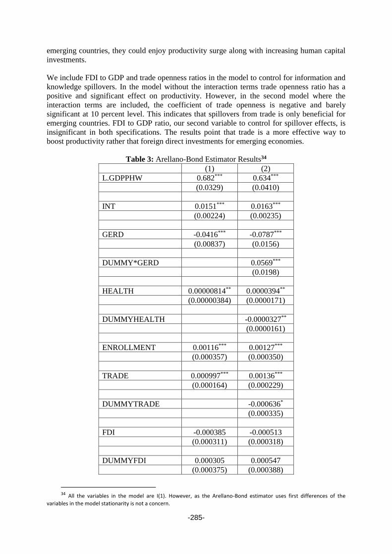
-285-

emerging countries, they could enjoy productivity surge along with increasing human capital

investments.

We include FDI to GDP and trade openness ratios in the model to control for information and

knowledge spillovers. In the model without the interaction terms trade openness ratio has a

positive and significant effect on productivity. However, in the second model where the

interaction terms are included, the coefficient of trade openness is negative and barely

significant at 10 percent level. This indicates that spillovers from trade is only beneficial for

emerging countries. FDI to GDP ratio, our second variable to control for spillover effects, is

insignificant in both specifications. The results point that trade is a more effective way to

boost productivity rather that foreign direct investments for emerging economies.

Table 3: Arellano-Bond Estimator Results34

(1) (2)

L.GDPPHW 0.682*** 0.634***

(0.0329) (0.0410)

INT 0.0151*** 0.0163***

(0.00224) (0.00235)

GERD -0.0416*** -0.0787***

(0.00837) (0.0156)

DUMMY*GERD 0.0569***

(0.0198)

HEALTH 0.00000814** 0.0000394**

(0.00000384) (0.0000171)

DUMMYHEALTH -0.0000327**

(0.0000161)

ENROLLMENT 0.00116*** 0.00127***

(0.000357) (0.000350)

TRADE 0.000997*** 0.00136***

(0.000164) (0.000229)

DUMMYTRADE -0.000636*

(0.000335)

FDI -0.000385 -0.000513

(0.000311) (0.000318)

DUMMYFDI 0.000305 0.000547

(0.000375) (0.000388)

34 All the variables in the model are I(1). However, as the Arellano-Bond estimator uses first differences of the

variables in the model stationarity is not a concern.

-286-

CONSTANT 1.298*** 1.481***

(0.128) (0.164)

N 432 432

Wald Test 13,634.74 2,020.78

p-value 0.0000 0.0000

A-B Serial Correlation

Test (First Order)

-2.5043 -2.4522

p-value 0.01 0.01

Sargan’s p-value 0.1685 0.2259

4. Conclusion and Policy Implications

In this study, we analyze the effects of digital economy and R&D on productivity. First, we

give information on industry 4.0 and discuss its possible channels to affect productivity such

as cloud computing, internet of things, and virtual reality. Then we analyze the determinants

of productivity with a special focus on digital economy by employing the Arellano-Bond

estimator for 24 OECD countries using data covering the 1995-2014 period. The dependent

variable we use is the natural logarithm of GDP per hour worked as it incorporates capital

goods, commodities, economies of scale, organization structure and technical advancement.

Since digital economy is fairly new in the literature and data are scarce we use natural

logarithm of internet users per 100 people and R&D expenditures to GDP ratio as proxies for

digital economy. We also use foreign direct investments to GDP ratio, natural logarithm of

health expenditures per capita (PPP-adjusted, constant prices), tertiary enrollment ratio and

foreign trade volume to GDP ratio as additional regressors.

It is found that internet users per 100 people contributes to productivity significantly.

However, R&D expenditures to GDP ratio, another proxy variable for industry 4.0, draws a

different picture. The effect of R&D expenditures on productivity is positive for advanced

countries and negative for emerging economies. It can be argued that some countries may use

public R&D funds ineffectively due to structural problems such as corruption, weak

institutions, inequality and injustice. This result urges emerging economies to improve their

institutions in order to build a more effective R&D program. It is also found that education

and health, the main pillars of the human capital investments, are effective to boost

productivity especially in emerging economies. Finally, we found that trade openness

significantly contributes to productivity whereas the effect of FDI to GDP ratio is

insignificant.

Our findings highlight the importance of productivity gains from digital economy and

industry 4.0 and provide important policy implications for policy makers, especially in

developing countries. Accordingly, improving indicators of digital economy such as the

number of internet users as well as human capital investments such as education and health

provide productivity gains for emerging economies. However, increasing the R&D spending

does not affect productivity if the country has weak institutions. Therefore, improving

institutions should be in the agenda of policy makers in emerging economies in addition to

increasing R&D expenditures.

.

-287-

REFERENCES

1. Arellano, M. and S. Bond. (April 1991). Some tests of specification for panel data: Monte

Carlo evidence and an application to employment equations. The Review of Economic

Studies, 58. pp. 277 – 297

2. Atasoy, Hilal (2011), ICT Use and Labor: Firm-Level Evidence from Turkey NET Institute,

Working Paper 11-23

3. Brynjolfsson,E and Hitt,L (1995) Information Technology as a Factor of Production:The

Role of Differences Among Firms , Economics of Innovation and New Technology, 3 (4

(Special Issue on Information Technology and Productivity Paradox)): pp. 183-200, (1995)

4. Chambers, Michele, Michael Minelli, Dhiraj Rajaram, and Ambiga Dhiraj (2012). Big Data,

Big Analytics, edited by Michele Chambers,et al., Wiley,

5. Crandall, Robert W., William Lehr, and Robert E. Litan. (2007). The effects of broadband

deployment on output and employment: A cross-sectional analysis of U.S. data. The

BrookingsInstitution: Issues in Economic Policy 6 (July)

6. Friess, Peter, and Ovidiu Vermesan (2013). Internet of Things, edited by Peter Friess, and

7. Ovidiu Vermesan, River Publishers,

8. Holtz-Eakin, D., W. Newey and H. S. Rosen (1988). Estimating vector autoregressions with

panel data. Econometrica 56. pp. 1371 – 1395.

9. ITU , The International Telecommunication Union (2016,) Facts and Figures ICT 2016,

http://www.itu.int/en/ITU-D/Statistics/Pages/facts/default.aspx, acces: 12.11.2016

10. Jorgenson, Dale W., Mun S. Ho and Kevin J. Stiroh. 2008. "A Retrospective Look at the U.S.

Productivity Growth Resurgence." Journal of Economic Perspectives, 22(1): 3-24.

11. Peitz, Martin, Gerhard Illing, (2006). Industrial Organization and the Digital Economy,

edited by Martin Peitz, et al., The MIT Press,

12. Shaw, Michael J. (2005) E-Commerce and the Digital Economy, edited by Michael J. Shaw,

Taylor and Francis.

13. Uhl, Axel, and Gollenia, Lars Alexander. Digital Enterprise Transformation : A Business-

Driven Approach to Leveraging Innovative IT. Farnham, GB: Routledge, 2014

14. Yilmaz, Serdar and Mustafa Dinc (2002) "Telecommunications and Regional Development:

Evidence From the U.S. States," Economic Development Quarterly, Vol. 16, No. 3 (August)

211-228.

-288-

AN INVESTIGATION THE RELATIONSHIP BETWEEN THE EXCHANGE

RATE VOLATILITY AND TOURISM RECEIPTS FOR TURKISH ECONOMY

Fatih Ayhan

University of Selcuk, Turkey


Fatih Mangir

University of Selcuk, Turkey


Abstract

Turkey has special coasts, touristic, historical and geographic facilities. So tourism has

special importance for Turkish economy, current account deficit is serious burden for Turkey

economy in recent years. Tourism receipt is an important tool for balancing the deficit and

also there are several positive externatilities of tourism for Turkey economy. In this paper,

exchange rate volatility and tourism receipt relationship is analyzed by theoratically and

emprically for the period of 2009M1-2016M9. Exchange rate volatility is calculated by

ARCH type model. After analyzing of series traditional unit root tests, the cointegration

relationship between the volatility and tourism receipt is investigated by the help of The

Bound Test approach and long term relationship is computed by ARDL model. According to

results, tourism receipt is positively affected by exchange rate level while exchange rate

volatility negatively affects the tourism receipt. But exchange rate volatility is statistically

insignificant.

Keywords: Tourism Income, Exchange Rate Volatility, Bound Test, ARCH.

1. Introduction:

Turkey has tough times in recent years both political and economic meaning. The Problems

arises from political issues such as terrorist attacks in southeast boundries, uneasiness in

Middle East, Syrian political situations, immigrant problems, Russian conflicts, problematic

relationship with EU. Besides its’ charming natural and historical beauties, tourism demand

for Turkey has exhibited a volatile performance in recent years because of political, economic

and financial concern. Although there are several economic determinants’ of tourism demand,

security problem creates main concern about it.

With this study, it’s aimed to determine the relationship between Exchange rate volatility and

tourism receipts’ of Turkey. This relationship is based on the trade and Exchange rate

volatility. In this relation, volatility in Exchange rate can be perceived as a risk factor and

uncertainty for economic future. Thus tourism demand reshaped by the line with risk

perceptions. Hovewer political unstability affects the tourism destinations and preferences. So

the factors beyond economic determinants can change the countries’ tourist potentials.

Tourism is multidimensional concept. It has social dimension about lesuire time and savings,

but it has also economic dynamics for example exports, budget and tax revenues, employment

opportunities, investment and consumption expenditures (Aktaş et al. 2014).



-289-

Tourism is heavily service-based sector and it provides enormous income for all economies.

This sector has lots of variations such as sport, cultural, health, historical tourism dimensions.

Thus investors preference to share huge budget for tourism. Tourism is a good chance for

developing countries to balance their deficit and it is a good choice to provide gains. Tourism

sector benefits can be specified as acceleration in development, extension in revenue,

increment in foreign Exchange, employment facilities, and tax revenues. So tourism positive

externalities on lots of sectors and we can say it has a multiplier effect on economy.

As the meaning of tourism, Turkey has some privileges, because it has special coasts,

surrounded by sea on three sides, hosted diffirent civilizations (Romans, Byzantine and

Ottoman Empires) that prodives cultural and historical gift to Turkey for higher touristic

demand. There is serious rivalry between the countries which have similar touristic

characteristics such as Spain, France, Greece, Italy and Turkey. To compete these countries, it

must be right and enough investment in touristic facilities. However, beyond the investment

problem, Turkish tourism sector needs to cope with its’ interior problems to compete its’

rivals such as security concerns, interior and outer conflicts, political problems with

neighbours etc. Advertisements of Turkish tourism sector are also crucial factor for the aspect

of development to tourism demand. It must be believed that Turkey is a safe country to travel

and it has a nice tourism quality.

After Bretton Woods Collapses, exchange rate uncertainty increased and its volatility.

Applying liberal programs and globalization causes to increase foreign trade after 1980s.

Tourism sector investment is growing rapidly and thus tourism demand and also tourism

receipts have increased recently. Thus changes in excange rate level affect the tourism

demand(Çağlar,2003). By the help of these changes, exchange rate and tourism relationship

being examined heavily in related literature. Tourism sector can be seen as a remedy lots of

economic problem for developing countries and so as a developing country, it’ll be examined

this relationship for Turkey economy with this paper.

Account deficit problem is the main concern of Turkish economy in recent years. She’s

coping with this problem since long time ago. Tourism receipts are an opportunity to balance

this deficit. However it is affected by exchange rate volatility. The main purpose of this paper

is to analyse the effects of exchange rate volatility on tourism receipts.

In this paper, the effects of exchange rate volatility on Turkey’s tourism receipts will be

analyzed by the help of co-integration analysis and error correction model. Datas are covering

the monthly data from January 2009 to September 2016. Firstly related literature review is

examined, and then the data and methodology are mentioned and findings and conclusion will

be submitted the last part.

2. Theoritical Backround:

General impacts of volatility can be summarized as: it’s accepted as an indicator for

macroeconomic instability and uncertainty. It causes to distrupting resource allocation,

decreasing foreign investment, decreasing economic growth and employment level. On the

contrary, in a the stable macroeconomic conditions provide; low and stable current account

deficit, Not real exchange rate loss, higher economic growth rate and incentive to new

investment decisions. So volatility in Exchange rate level is unpleasant action for the

economic actions.

-290-

Main argument behind the tourism receipts and volatility relationship is based on the

exchange rate and foreign trade relationship. If exchange rate volatility increases, foreign

trade decreases according to risk perception. So the same logic is valid about the relationship

between the tourism receipts and exchange rate volatility. When exchange rate level

increases, local tourism costs become cheaper and tourism demand increases. Thus total

tourism receipts accelerate. On the contrary, if exchange rate level decreases, local tourism

becomes costly and tourism demand also decreases (Şen and Şit, 2015).

There are various determinants that affect the tourist arrivals and tourism receipts. These

factors can be economic, social, political, endogenous and exogenous. The main socio-

economic determinants of tourism demand can be summarized as; (Agiomirgianakis (2012);

Garin-Munoz (2000) and Patsouratis, et. al. (2005), Anderson and Van Wincoop,2003:

Gallego et al,2010:30))

✓ Cost of living in target country and relative cost of living differences between

the countries,

✓ Transportation costs and distance of travelling route,

✓ Quality of touristic facilities,

✓ Language, traditions, attitudes towards to tourists,

✓ Market size (GDP) and economic development of host country,

✓ Inflation of local country,

✓ Availability of labour and labour costs,

✓ Availabilty of natural, cultural, social and hictorical facilities,

✓ Real exchange rate level and macroeconomic uncertainty,

✓ Security concerns inside and near boundries.

There are several crucial benefits of tourism sector to economy. Tourism helps to decrease

balance of payment deficit. Tourism sector is a source of employment creation. This sector is

dominantly consisting of service sector and also satisfies the unemployed persons’ job needs.

Tourism provides exchange to economy and thus tourism remarkably affected by exchange

rate fluctuations (Demirel et.al.,2013:117).

Tourism is multidimensional and socio-economic concept. It has social dimension about

leisure time and savings, but also it has economic dynamics. These are summarized as; it

increases the export and tax revenues, balances the budget deficits, provides new employment

opportunities, makes contributions the investment, increases the total consumption level and

enchances the interactions between the cultures (Aktaş et al. 2014).


According to empirical studies, different results obtained from many papers. Some papers

found negative result between Exchange rate and tourism receipts while others had positive

and also some papers couldn’t found any relation between them. These results can be

explained by the help of methods, data, period, countries’ tourism and economic Dynamics

that used in their analysis.

Tourism demand and exchange rate volatility relation is theoretically based on the foreign

trade and exchange rate relationship. Foreign trade is negatively affected by exchange rate

volatility according to theorical and empirical studies (Clark (1973), Hooper and Kolhagen

(1978), Kenen and Rodrik (1986), Koray and Lastrapes (1989), Dellas and Zilberfarb (1993),

Arize (1997), Mckenzie (1999), Clark et.al.(2004) Takaendase et.al. (2005), Öztürk(2006)).

-291-

Bahmani and Wang (2007), Byrne et.al.(2008), Altıntaş and Öz (2010), Özdemir and Ordu

(2013). Thus similar relationship is valid for the tourism receipts and related literature review

is as follows and summarized at Appendix.1.

When we looked at the related empirical literature, we can classify the studies according to

their results. The studies that found negative relation and co-integration relationship between

the exchange rate level, volatility and tourism receipts. These are summarized as Webber

(2001), Garin-Munoz and Perez-Amaral’s study (2000), Eilat and Einav (2004) Demir and

Toker (2012). However some emripical studies couldn’t reach any significant relationship

between them. These are Eugenio-Martin and Morales (2004) Mervar and Payne (2007),

Demirel et.al.(2013). Detailed literature review is submitted the Appendix.1.

4. Data And Methodology

It‘s used monthly data covering the period from 2009:M1 to 2016:M9. Tourism receipts

includes the international tourist expenditures in Turkey. Exchange rate variable captures the

producer price index based real effective exchange rate.

Exchange rate variables are obtained from Turkey Central Bank database system. Tourism

receipts captured from TurkStat, Central Bank, Ministry of Culture and Tourism. In the

empirical model; Tourism receipt (TRCP) is explained by exchange rate and it’s volatility

parallel with the existing literature. For exchange rate volatility (VOL), conditional

heteroscadasticity of ARCH type models are calculated.35

In the empirical modelling, TRCP is explained with exchange rate level and its’ volatility in

accordance with the related literature.

Empirical analysis is started with the stationarity analysis. Ng Perron tests are used for this

purpose. Co-integration relationship between the variables investigated by the help of Bound

test approach that proposed by Peseran et. al (2001) and superior properties than conventional

co-integration models after stationarity control. When series are different level of stationarity,

we can simply use the Bound Test in order to analyse cointegration relationship (Pesaran et al.

2001; Narayan and Narayan, 2004). The co-integration checking, the long and short run

elasticities between variables are calculated by ARDL model in the following section.

5. Results

5.1 Stationarity Analysis

We used Ng-Perron test in order to determine stationarity level of series. As Ng-Perron test

has more powerful features than other tests such as ADF and PP tests. According to Ng-

Perron test results LTRCP series is found I(1) and VOL series also are found I(0).

35 ARCH type model for real exchange rate is chosen as the best performed model in this study. Conditional variance is obtained from

ARCH model is used as an exchange rate volatility variable for the model. Comparison for estimated coefficients and model forecasting performances are not presented here in order to keep the study compact. The model results could be obtained from the authors, if needed.

-292-

5.2 Cointegration Analysis

Unrestricted Error Correction Model (UECM) should be set up in order to use Bound test

after the stationarity control. Thus UECM model specification for this paper is set up as in

equation (1).

tttt

m

i

iti

m

i

iti

m

i

itit VOLaLERaLTRCPaVOLaLERaTRCPaaLTRCP

161514

1

3

1

2

1

10

(1)

In equation (1); m represents lag number.36 It’s checked the co-integration relationship by

using the F test and null hyptesis established as 087650 aaaaH after the determination

of lag number for the UECM model. When we compared the calculated F-statistic that

retrieved from UECM models’ critical levels in Pesaran et al. (2001), the estimated F statistics

is bigger than the upper bound. So we can reject the null hypothesis of no co-integration. If

the estimated F statistics is smaller than the bottom bound, there can’t be co-integration

relationship between the variables (Narayan and Narayan, 2004). If the calculated F statistics

is among the boundries, the result can be assumed as inconclusive (Karagöl et.al.,2007).

Table 1: Bound Test

K F statistics

Critical Value at %5

Significance Level

Bottom

Bound

Upper

Bound

2 13.08001 3.79 4.85

According to Table 1, F statistics is greater than the upper bound of the critical values, and the

null hypothesis of no co-integration is rejected. As a result, we found a significant long run

cointegration relationship between the variables.

5.3. ARDL Model

The long and short run static relationship between the variables will be analyzed with ARDL

model after the co-integration control. ARDL models’ of our study is presented as in equation

2.

t

m

i

iti

l

i

iti

k

i

itit VOLaLERaLTRCPaaLTRCP

1

3

1

2

1

10 (2)

The best ARDL model is selected as ARDL(2,1,0). k, l, m and n symbolizes the lag numbers

in eq.2. The estimated long and short term coefficient using ARDL (2,1,0) model are shown

in Table.2. Error terms in ARDL model has no serial correlation, heteroscedasticity and

misspecification problems according to diagnostic check results that can be seen in Table.2.

Table.2 ARDL (2,1,0) Model’s Long And Short Term Coefficients

ARDL (2,1,0) Model’s Long Term Coefficients

Variables Coefficie

nts

t Statistic

LKUR 1.199361 3.470441

VOL -109.98163 -0.372895

C 4,471167 0,653004*

36 Maximum length is accepted as 5 and according to Akaike and Schwarz criterions lag number is accepted as 1 in this paper. And

also it’s examined whether or not autocorrelation problem through LM test in UECM model which formed with 1 lag number, autocorrelation isn’t defined with 1 lag number.

-293-

ARDL (2,1,0) Model’s Error Correction Coefficient

Variables Coefficie

nts

t Statistic

ECMT(-1) -0,063026 -3,210411

ARDL (2,1,0) Model’s Diagnostic Checks

BGX 2 1.861[0,80]

2

WHITE 0.782[0,37]

RAMSEYX 2 1,151[0,15]

BGX 2

, 2

WHITE, RAMSEYX 2

are accordingly shows autocorrelation, heteroscadasticity and

Ramsey tests. Probability values are in brackets.

Note: *%1,**%5 shows significance level.

According to long term coefficients obtained from ARDL (2,1,0) model, exchange rate level

have positive effect on tourism receipts, while exchange rate volatility has negative effect on

it, however it’s not statistically significant. The results are sutiable for the related literature.

Error correction coefficient is calculated as -0,06 and it shows the deviation from short and

long run equilibrium.

6. Conclusion

Tourism sector is growing and beneficial sector which has lots of solutions to economic

problems such as exchange deficit, balance of payments, employment need etc. Tourism

secter is affected by socio-economic variables. So exchange rate level and its’ uncertainty

affects the tourism demand and also tourism receipts of countries.

In this study, the relationship between exchange rate volatility and Turkey’s tourism revenues

was examined. As an econometric model, firstly exchange rate volatility has been estimated

with the ARCH approach; then, the relationship among tourism revenues was investigated by

including error correction model. It‘s used monthly data covering the period from 2009:M1 to

2016:M9. Tourism receipts includes the international tourist expenditures in Turkey.

Exchange rate variable captures the producer price index based real effective exchange rate.

According to the results obtained from the model, exchange rate level have positive effect on

tourism receipts, while exchange rate volatility has negative effect on it, however it’s not

statistically significant. The results are sutiable for the related literature. Error correction

coefficient is calculated as -0,06 and it shows the deviation from short and long run

equilibrium. These results shows that exchange rate level is a crucial determinant of tourism

receipts for Turkey, however exchange rate volatility hasn’t got any importance about it. We

can assume that the other factor which affects the tourism demand is much more dominant

than the volatility.

-294-

APPENDİX.1 Related Literature Review

Author(s) Country(ies) Period Variables Methods Results

Webber

(2001) Avustralia

1983:1-

1997:4

Foreign tourism

demand and exc.rate

Johansen and

Engle& Granger

procedures

A change in ER explains the %50 of tourism

demand in the long run.

Salman

(2003) Sweden

1980:1-

1998:12

Tourism demand,

income, price, ER

Chernobil nuclear

accident dummy, 1991

Gulf War dummy

Co-integration

analysis

Income, ER and consumer price index are effective

for the aspect of international touristic demand.

Eugenio-

Martin and

Morales

(2004)

Latin

American

Countries

1985-1998 Economic growth and

tourism receipts Panel Data analysis

Between the ER, PPP and tourism receipts has NOT

significiant relationship.

Dritsakis

(2004) Greece

1960:I-

2000:IV

Real GDP, REER and

international tourism

receipts

VAR model There is a long run relationship between the RER

and international tourism receipts.

Patsouratis

vd. (2005)

Mediterrian

Countries 1990-2004

Income index, host

countries’ price index,

rivals’ price index and

ER

(Spain, Portugal and

Italy)

Panel Data Anlysis It’s determined that main determinant for Greece’s

tourism demand are price index and ER.

Mervar and

Payne (2007) Crotia 1994-2004

Tourism income and

ER ARDL Analysis

RER doesn’t have any effect on tourism demand

according to results.

Özçelebi

(2009) Turkey

1992:01-

2009:03

Tourism expenditure,

Real GDP and RER.

Vector Error

Correction Model

There is not a significiant relationship in the short

run. Hovewer there is a significiant long run

relationship between the Real GDP, ER and tourism

expenditures.

Arsad and

Johor (2010) Malaysia

1999:1-

2008:9

Relative prices, ER,

Trasportation costs,

Relative costs of

Co-integration

analysis

When devaluation and relative costs of rivals’

destinations have positive effects on tourism

inflows, transportation cost increment has negative

-295-

rivals’ destinations

and tourism demand

one.

Uğuz and

Topbaş

(2011)

Turkey 1990:1-

2010:12

RER, Volatility and

tourist demand

Johansen

Cointegration

Analysis

There is a significiant and long run relationship

between the tourism demand, ER and ER volatility.

Demir and

Toker (2012) Turkey 1980-2010

Tourist arrivals, RER,

Volatility, Trade

volume, 1994-2001

Shock dummies

VECM Analysis

It is found that tourism demand was affected

negatively by ER volatility in the short and long

run. However it wasn’t affected by financial crises.

Demirel

et al(2013) Turkey

1994:1-

2006:4.

Real Exchange Rates

and the uncertainty,

number of tourists

Cointegration

Analysis

With respect to the uncertainty in real exchange

rates, the uncertainty does not have any effects on

the number of tourists, except for France.

Cheng et.al.

(2013) USA 1973-2010

RER and tourism

receipts. VAR Analysis

Increment in RER

affects the USA’s

tourism receipts

Aktaş et al,

2014 Turkey

2003:1-

2011:12.

Effects of exchange

rate volatility on

tourism revenues.

Co-integration

analysis

Exchange rate volatility has a negative effect on

tourism revenues. Additionally, a weak relationship

was detected in the long term between exchange

rate and tourism revenues.

Agiomirgian

akiset al.(

2015)

Iceland 1990:1-

2014:4.

ER volatility and

Tourist arrivals

Co-integration

analysis

There is a negative effect of volatility to tourists’

arrivals for Iceland.

Şen and Şit

(2015) Turkey

2000:1-

2012:12

RER and Tourist

receipts reel

Toda-Yamamoto and

Bootstrap based

Toda-Yamamoto

cointegration

analysis

According to results, RER has a significiant effect

on the Turkey’ tourism receipts. And tourism

receipts also affect the RER.

-296-

REFERENCES

1. Aktaş Ali Rıza, Burhan Özkan, Fatih Kaplan and Robin Gail Brumfield, (2014). Exchange Rate

Volatility: Effect on Turkish Tourism Incomes, Management Studies, August 2014, Vol. 2, No.

8, 493-499.

2. Anderson, J.E., and Van Wincoop, E. (2003), ‘Gravity With Gravitas: A Solution To The Border

Puzzle’,American Economic Review, Vol 93, No 1, pp 170–192.

3. Arsad ve Johor (2010) Arsad, Z. ve Johor, N.B.M. (2010). Estimating European Tourism

Demand For Malaysia. World Academy of Science, Engineering and Technology, 66, 1606-

1611.

4. Cheng Ka Ming, K.; Hyeongwoo H., Thompson. 2013. “The Real Exchange Rate and the

Balance of Trade in US Tourism”, International Review of Economicsand Finance 25: 122–128

5. Clark, P.B., Tamiris, N., and Wei, S.-J. (2004), ‘A New Look At Exchange Rate Volatility And

Trade Flows’, IMF Occasional Paper 235.

6. Çağlar, Ünal (2003); Döviz Kurları- Uluslararası Para Sistemi ve Ekonomik İstikrar, Alfa

Yayıncılık, İstanbul.

7. Demir Çiğdem and Boran Toker (2012). „Finans Piyasalarındaki Döviz Kuru Oynaklığının

Turizm Talebine Etkisi : Türkiye Örneği“, International Istanbul Finance Congress-2012, 13-

14th June 2012, Okan University, İstanbul.

8. Demirel Baki, Barış Alparslan, Emre Güneşer Bozdağ and Alp Gökhun Inci, (2013). The

Impact Of Exchange Rate Volatitility On Tourism Sector: A Case Study, Turkey, Niğde

Üniversitesi İİBF, 6:2, 117-126.

9. Dritsakis (2004) Dritsakis, N. (2004), Tourism as a Long-Run Economic Growth Factor: An

Empirical Investigation for Greece Using Causality Analysis. Tourism Economics, 10, 305-316.

10. Eilat, Y., & Einav, L. (2004). Determinants of international tourism: A three-dimensional panel

data analysis. Applied Economics, 36, 1315-327.

11. Eugenio-Martin and Morales (2004) Eugenio-Martin, J.L. ve Morales, N.M. (2004). Tourism

and Economic Growth In Latin American Countries: A Panel Data Approach”, Nota Di Lavoro,

26.

12. Gallego María Santana, Rodríguez Francısco J. Ledesma and Rodríguez Jorge V. Pérez (2010).

Exchange Rate Regimes And Tourism, Tourism Economics,16 (1), 25–43.

13. McKenzie, M.D. (1999), ‘The impact of exchange rate volatility on international trade flows’,

Journal of Economic Surveys, Vol 13, No 1, pp 71–106.

14. Mervar ve Payne (2007) Mervar, A. ve Payne, J. (2007). Analysis of Foreign Tourism Demand

For Croatian destinations: long-run elasticity estimates. Tourism Economics, 13, 407-420.

15. Narayan (2004) Narayan, P.K. (2004). Economic Impact Of Tourism On Fiji's Economy:

Empirical Evidence From The Computable General Equilibrium Model. Tourism Economics,

10, 419-433.

16. Özçelebi, O. (2009). Outbound tourism demand in Turkey: a Vector Error Correction Approach.

The Business Review, Cambridge, 13 (2), 310-317.

17. Ozturk, I. (2006), ‘Exchange Rate Volatility And Trade: A Literature Survey’, International

Journal of Applied Econometrics and Quantitative Studies, Euro-American Association of

Economic Development, Vol 3, No 1, pp 85–102.

18. Patsouratis vd. (2005) Patsouratis, V. Frangouli, Z. ve Anastasopoulos G. (2005). Competition in

Tourism Among The Mediterranean Countries. Applied Economics, 37, 1865-1870.

19. Salman (2003) Salman, A.K. (2003). Estimating Tourist Demand Through Cointegration

Analysis: Swedish Data. Current Issues in Tourism, 6(4), 323-339.

-297-

20. Şen Ali and Mustafa Şit (2015). „Reel Döviz Kurunun Türkiye’nin Turizm Gelirleri Üzerindeki

Etkisinin Ampirik Analizi [The Empirical Analysis of Real Exchange Rate Impact on Turkey’s

Tourism Receipts], Journal of Yasar University, 2015, 10/40, 6752-6762.

21. Uguz Sabriye Çelik and Ferhat Topbas (2015). Döviz Kuru Oynaklıgı Turizm Talebi iliskisi:

1990-2010 Türkiye Örnegi [Relationship between Exchange Rate Volatility and Tourism

Demand: Case Study in Turkey for the Period of 1990-2010], Paper presented at EconAnadolu

2011: Anadolu International Conference in Economics II, June 15-17, 2011, Eskisehir, Turkey.

22. Webber, A.G. (2001), ‘Exchange Rate Volatility And Cointegration In Tourism Demand’,

Journal of Travel Research, Vol 39, No 4, pp 398–405.

23. Enders, W. (1995). Applied econometric time series (p. 239). New York: John Wiley & Sons

Inc..

24. Engle, R. F. (1982). .Autoregressive conditional heteroskedasticity with estimates of the

variance of United Kingdom inflation. Econometrica, 50, 987-1007.

25. Engle, R. F., & Granger, C. W. J. (1987). Co-integration and error correction: Representation,

estimation and testing, Econometrica, 55, 251-276.

26. Garin-Munoz, T., & Perez-Amaral, T. (2000). An econometric model for international tourism

flows to Spain. Applied Economics Letters, 7, 525-529.

27. Gomez, V., & Maravall, A. (1998). Seasonal adjustment and signal extraction in economic time

series (Bank of Spain, No: 9809).

28. Granger, C. W. J. (1988). Some recent developments in a concept of causality. Journal of

Econometrics, 39, 199-211.

29. Green, W. H. (2002). Econometric analysis (5th ed.). Saddle River: Prentice Hall.

30. Gujaratin, D. (2009). Basic econometrics (pp. 713-726). Istanbul: Literature Publishing.

31. Johansen, S., & Juselius, K. (1990). Maximum likelihood estimation and inference on

cointegration-with application to the demand for money. Oxford Bulletin of Economics and

Statistics, 52, 169-210.

32. Nelson, D. B. (1991). Conditional heteroskedasticity ın asset returns: A new approach.

Econometrica, 59, 347-370.

33. Takaendesa, P., Tsheolet, T., & Aziakponoa, M. (2005). Real exchange rate volatility and its

effect on trade flows: New evidence from South Africa. Proceedings from Biennial Conference

of the Economic Society of South Africa.

34. Tse, R. Y. C. (2001). Estimating the impact of economic factors on tourism: Evidence from

Hong Kong. Tourism Economics, 7, 277-293.

35. Agiomirgianakis George, Dimitrios Serenis and Nicholas Tsounis (2015), Effects of Exchange

Rate Volatility on Tourist Flows into Iceland, International Conference on Applied Economics,

ICOAE 2015, 2-4 July 2015, Kazan, Russia.

36. Öztürk, İlhan. (2006). Exchange Rate Volatility and Trade: A Literature Survey. International

37. Journal of Applied Econometrics and Quantitative Studies, 3(1), 85-102.

38. Takaendase, P., Tsheole, T. ve Aziakpono M. (2005). Real Exchange Rate Volatility and Its

39. Effect On Trade Flows: New Evidence From South Africa, The Biennial Conference of The

40. Economic Society of South Africa, Durban, 1-20.

-298-

RISK-SHARING BANKING: VIABILITY AND RESILIENCE

Siti Muawanah Lajis

Bank Negara Malaysia, Malaysia


Abbas Mirakhor

INCEIF, Malaysia

Abstract

The present Islamic banking model is inherently fragile owing to its unmatched balance sheet

which exposes the banks to various risks on daily basis. To mitigate the risks, similar to the

conventional banks, Islamic banks operate on risk-transfer mode where risks are transferred to

the counterparty or the public. Risk-transfer banking however induces negative behaviors such as

excessive risk taking and socially unproductive financial intermediation. This paper proposes

risk-sharing based banking model where the balance sheet are matched in terms of maturity,

value, risk and materiality. The risk-sharing model is envisaged to provide the opportunity for

Islamic banks to completely move away from risk-transfer banking mode. It offers greater

stability, firmly anchors banking sector to real economy, has greater resilience to shocks, and

capable of reducing financial oppression and predatory lending. As such, this paper undertakes an

empirical investigation to illustrate the viability and resilience of risk-sharing model vis-à-vis the

risk-transfer model. The methodology used is simulation of balance sheet and the results are

stress tested.

Keywords: Risk sharing, risk transfer, balance sheet, simulation, stress test

1. INTRODUCTION

The present business model of Islamic banks is inherently fragile due to its unmatched balance

sheet structure exposing the banks to daily liquidity and maturity risks. To mitigate the risks, the

Islamic banks engage in risk-transfer based financial intermediation where risks arising from

financial transaction are transferred or shifted to the counterparty or the public. At transactional

level, credit enhancements or collaterals are common safety measures to mitigate credit/ liquidity

risks. At institutional level, the Basel capital adequacy framework is widely adopted as

mechanism to address asset impairments. At systemic level, deposit insurance and implicit/

explicit government guarantee schemes are meant to enhance the soundness of the banking

system against sudden bank runs or shocks. At the same time, risk-transfer banking induces

negative behaviors such as excessive risk taking and socially unproductive financial

intermediation.

Risk-transfer model diverges away from the ideal Islamic banking which is premised on risk-

sharing principles. Malaysia via the Islamic Financial Services Act 2013 (IFSA), the central

bank’s guidelines to ring-fence investment account and the internet-based investment account

platform (IAP) are recent initiatives to promote risk-sharing finance. The adoption of the risk-

sharing model could serve as the main differentiating factor for Islamic banks as the banks

-299-

completely move away from risk-transfer banking mode. The risk-sharing model could

potentially create a new value creating asset class for Islamic banks and investors through real

sector-linked investment intermediation. It may also offer greater stability and resilience than the

risk-transfer model. In this regard, this paper undertakes an empirical investigation to compare

the two models. The rest of the paper is organized as follows. Section 2 explains the data and

methodology, Section 3 discusses the findings of the research, Section 4 reports the outcome of

the stress testing and Section 5 concludes the research.

2. METHODOLOGY

This empirical investigation and simulation exercise involves a three-step process. Step 1

illustrates the profiles of the mismatched (risk-transfer banking model) and matched (risk-sharing

model) balance sheet structure. Step 2 estimates the rate of return of the real sector. Step 3 makes

a comparison on the potential profits generated under the two models. The procedures are further

explained as follows.

2.1 Step One

The aim is to construct two stylized balance sheets of a representative bank (RB). Two sets of

data are used – (i) financing representing the asset and (ii) risk bearing deposits namely the

special investment account (SIA) and general investment account (GIA) representing liability.

Data are sourced from the Bankscope comprising 16 Islamic banks in Malaysia for period 2007-

2013. These data are then converted using the weighted average of each bank’s balance sheet in

proportion to the total industry to derive the balance sheets of the RB. The rationale for this

exercise is to incorporate the balance sheet profiles of all Islamic banks without singling out any

one of them. The detailed steps undertaken involved the following:

● Determining each bank’s weights (wi) by dividing its total assets and total liabilities with

those of the respective industry’s aggregates.

● Then each bank’s weights are multiplied with its own total assets and total liabilities to

derive its allocation of assets and liabilities.

● The representative bank’s total assets and total liabilities are derived by adding the values

of the 16 banks’ weighted total assets and weighted total liabilities.

Next, the asset and liability are grouped into three time buckets (i) short-term with less than 1

year tenure, (ii) medium-term with 1 to 3 years tenure and (iii) long-term with more than 3 years

tenure. The outcome of this is the balance sheet structure of the present Islamic banking model

(risk-transfer mode).

The first balance sheet keeps the existing mismatched structure depicting the current risk-transfer

model. The second balance sheet is re-configured based on a matched asset-liability structure to

illustrate risk-sharing model. This exercise involves two fund management processes (1) asset-

liability matching and (2) asset-real sector tagging. The asset-liability matching ensures that risks

are mitigated by way of a one-to-one matching of the liabilities (deposits/investments) against the

assets (financing) in terms of maturity, value and risk – the first three conditions for risk sharing

(Mirakhor, 2015). The outcome of this is an asset-driven mobilization of resources. Investment

ownership is represented by the individual acquisition of low-denominated securities that are

tradable in secondary markets. Meanwhile, the asset-real sector tagging ensures that investment

-300-

intermediation between surplus and deficit unit of the economy is optimized; and that the

financial sector is linked to productive economic activities. Such arrangements are necessary to

achieve the fourth condition of risk sharing - materiality.

2.2 Step Two

The objective is to derive the rate of return (ROR) of the risk-sharing securities to visualize the

prospect on investors’ compensation. However, because there is presently no such market and

instrument, a proxy (ROR of the real sector) is derived as follows.

● Obtaining all equities from Bursa Malaysia (Source: Thomson Reuters IEKON)

● Selecting only Shari’ah compliant companies with positive performances

● Extracting the ROR for selected companies and compute portfolio ROR

● Applying portfolio ROR to risk-sharing Balance Sheet

The outcome of this exercise is the ROR of the securities. The ROR estimation involved a 10-

step procedure summarized in the following diagram.

Figure 1: Process for Estimating ROR

Source: Author’s own

2.3 Step Three

The objective is to empirically prove that investment in real sector promises superior returns than

the banks’ interest rate-based returns. As an illustration, a comparison on the deposit and

financing rates of Islamic banks (source: BNM Quarterly Bulletin) are made against the derived

ROR of the risk-sharing securities. The differential rates would give an indication on how much

the investors would have benefited should Islamic banks channel the SIA and GIA to the real

sector. Similarly, the differential rates between the financing rates and the ROR of the real sector

give an indication how much Islamic banks would have forgone on the upside potentials in the

real sectors.

-301-

2.4 Limitation

The main limitation of this study is the unavailability of data for the ROR of real sector. In its

absence, the Return on Long Term Assets was used as proxy hence rendering this study as a

rudimentary illustration of an ideal risk-sharing banking model.

3. RESULTS

3.1 Balance Sheet Profiles

Figure 2: Asset-Liability Mismatch in Present Balance Sheet Structure


The analysis on the balance sheet structure under the risk-transfer banking model revealed several

pertinent issues. The first observation was a strong evidence of maturity transformation of the

asset and liability where Islamic banks are seen to “lend long and borrow short”. Commonly

known as an Asset-Liability Mismatch, this phenomenon is prevalent even in Islamic banking

simply because the function of banking has been limited to taking deposits (which are short-term

in nature) and making loans/financing (typically long-term). In the case of Islamic banking in

Malaysia, about 80% of short-term SIA and GIA are channeled to 80% of long-term assets. This

mismatched balance sheet structure typifies the banking model of risk-transfer system. Its main

weakness is the inherent fragility to shocks, either by increased funding cost or sudden

withdrawals which subject it to continuous exposure to liquidity, credit and market risks. In event

of a sharp increase in interest rate, the impact can be significant.

Due to the inherent mismatch of assets and liabilities, banks need to continuously rearrange the

assets and liabilities to obtain optimal returns while providing adequate liquidity and capital, as

well as ensuring interest rate sensitivity characteristics of the bank’s assets and liabilities are

within the bank’s risk appetite. This process of addressing the mismatch risks is called the Asset

Liability Management (ALM).

The second observation is the persistent trend to over-concentrate on household financing,

averaging about 60% of total Islamic banking financing. By concentrating on a certain sector,

risks are being concentrated and hence not well diversified. As seen in Figure 3 below, this

-302-

financing preference matter-of-factly typifies the character of risk-transfer system. The high level

of household credit could pose a threat to the stability of the overall financial system. It is worth

noting that similar trend is also observed in many countries. It is believed that such trending has

been influenced by the incentive structure of the present regulatory regime. The Basel capital

requirements on risk-weighted assets induce preference for debt type of financing in the low or

risk-free asset class. Households are a low risk asset class given the credit enhancement and

safety net mechanism, even though household financing is generally less productive than

enterprise/corporate finance. By engaging in household financing, Islamic banks virtually transfer

all of their credit risk to the borrowers by having the financing to be backed by collateral and

assigned wages. Because of this, Islamic banks are not incentivized to develop investment

expertise and capability to deploy risk-averse risk-sharing to businesses. The untapped segments

of the economy such as start-ups, budding entrepreneurs and SMEs thus remain underserved.

Inadequate investments in productive activities would in the long run undermine the development

of the economy.

Figure 3: Financing by Sectors

Source: Bank Negara Malaysia, Monthly Statistical Bulletin

As shown in Figure 4, the third observation is the dominance of debt-based contracts (Bay’

Bithaman Ajil (BBA), Ijarah Thumma al-Bay’ (AITAB) and Murabahah) as the main

instruments for Islamic banking assets. In addition, hybrid contracts classified under others are

showing an increasing trend. These are essentially pseudo-debt instruments designed to fit into

the risk-transfer operating mode. On the other hand, equity based financial contracts

(Musharakah and Mudharabah) are used minimally. This finding is in line with various studies

such as by Ali (2010), Rosly (2007) and Ali & Ahmad (2006). Rosly (2007) noted that despite

having the universal banking license, Islamic banks licensed under IBA 1983 had not pursued the

non-traditional banking services such as insurance (takaful), leasing (ijarah), stockbroking

(wakalah), unit trusts (wakalah-mudarabah), underwriting (al-bay’) and equity (musharakah).

-303-

The main reason for shying away from equity-based instruments is the lack of appetite for riskier

assets. Such reservation stems from Islamic banks trying to emulate the business model of

conventional banks (Askari et al, 2012). The domestic legal, regulatory, tax and accounting

framework and Basel capital requirements seek to shift protection of depositor’s principal to

governments and induce a lack of appetite for risk-sharing instruments.

Figure 4: Financing by Contracts from year-end 2007 to 2014 (RM million)

Source: Bank Negara Malaysia, Monthly Statistical Bulletin

Debt finance is permitted in Islam provided that it is appropriately originated [i.e. through real

economic activity] and structured [i.e. avoiding all elements of riba, maysir and gharar]. It

should be emphasized also that a balanced usage of debt-and equity-based finance needs to be

prescribed so as to ensure that the value proposition of Islamic finance is fully realized. This

stance is confirmed by the Kuala Lumpur and Jeddah Declarations and other pronouncements

(including evidence-based prescriptions from non-Muslim economists). Presently, debt-based

instruments are used in almost all financing transactions, whilst the use of equity-based

instruments is minimal. As a result, the real economy linkages of Islamic banking are tenuous.

Financial instruments are priced based on the prevailing OPR and not based on the risk-reward

profile of the underlying projects that are being financed. Because of the decoupling, financial

instruments are often mispriced. In post GFC rate environment where interest rate is much lower

than the return in the real sector, the credit spread adjustments rather than sharing in venture’s

real profitability is significantly higher.

Furthermore, the over reliance on debt instruments also induces moral hazard on the part of banks

as the financier. As risk-transfer returns are non-state contingent and collateralized, banks’

-304-

incentives to lend to the limit to maximize their leveraged-based returns leads to adverse

selection problems and poor monitoring.

The implication of banking sector being heavily based on debt and by being the main conduit for

money supply is that the whole economy and financial system have become highly leveraged,

with high debt and low equity. In this scenario, the risk is completely shifted to the system as a

whole, whereas the real sector bears all risks if the financial system collapses (Mirakhor, 2014).

Figure 5 below illustrates the simulation result of a matched balance sheet for risk-sharing model.

Both the asset and liabilities are now matched in terms of materiality, maturity, value and risk.

This effectively leads to liquidity, credit and market risks being avoided, hence the balance sheet

is intrinsically more stable and less sensitive to external shocks. Also as financing is linked to the

real sector, the size of financing will tend to correspond with the expansion of the real sector.

Figure 5: Matched Balance Sheet in Risk-Sharing

Model

3.2 Deriving Rate of Return (ROR) for Risk-sharing Securities

The following step is to derive the price of the securities. However as such a market price is not

yet in existence, we have used a simplistic proxy based on the performance of actual companies

listed in Bursa Malaysia represented by their rate of return (ROR). Since information on

companies’ ROR is not readily available, we manually estimated the ROR using the return on

long-term assets (ROLA) of the Shari’ah compliant companies publicly listed at Bursa Malaysia

selected as the proxy. ROLA is calculated as Net Income Before Tax (NIBT) divided by Long

Term Assets. Prior to calculating the ROR, we first selected the companies.

-305-

Figure 6: Publicly Listed Companies on Bursa Malaysia Exchange (1999-2013)

Source: Thomson Reuters Eikon

A total of 896 companies representing all the 10 economic sectors in Malaysia were screened

involving a two-layer filtering: (i) omitting companies with negative and greater than 100%

ROLA for the whole 15 years, and (ii) companies with negative and greater than 100% ROLA for

the last five years are omitted. After two rounds of filtering, 424 companies were finally selected.

We consider ROLA a fair proxy on the basis that they are typically the earning assets of

companies. The estimated ROR based on ROLA was 20.98%. After adjusting to portfolio risk of

0.98%, the risk adjusted ROR was 20.77%. In order to check the reasonableness of the derived

ROR, other estimations based on the return on total assets (ROA) and the pre-tax return on equity

(ROE) were also made. The returns based on ROA and ROE were 12.48% and 19.50%

respectively. In addition to these proxies, we also referred to other estimates of the real sector

returns from secondary sources. The Morningstar reported that the average returns of the top 100

companies in the world are in the range of 15% (for 3-year average) and 14% (5-year average)37.

Studies had proposed that the equity premium in Malaysia is in the range of 8 to 11% (Mirakhor,

2015). Meanwhile, AIBIM38 in 2015 reported that the potential return of real sector estimated by

the banking fraternity is in the range of 11 to 18%.

Table 1: Estimated Rates of Return of Real Sector

Proxy ROR

Estimation

Return on Long-term Assets (ROLA)

20.98%

Return on Total Assets (ROA)

12.48%

Return on Pre-tax Equity (ROE)

19.50%

Average Return of Top 100 Global Companies*

13% -

15%

Equity Premium in Malaysia 8 - 11%

37 Bacha & Mirakhor (2015) 38 AIBIM is the Association of Islamic Banking Institutions Malaysia

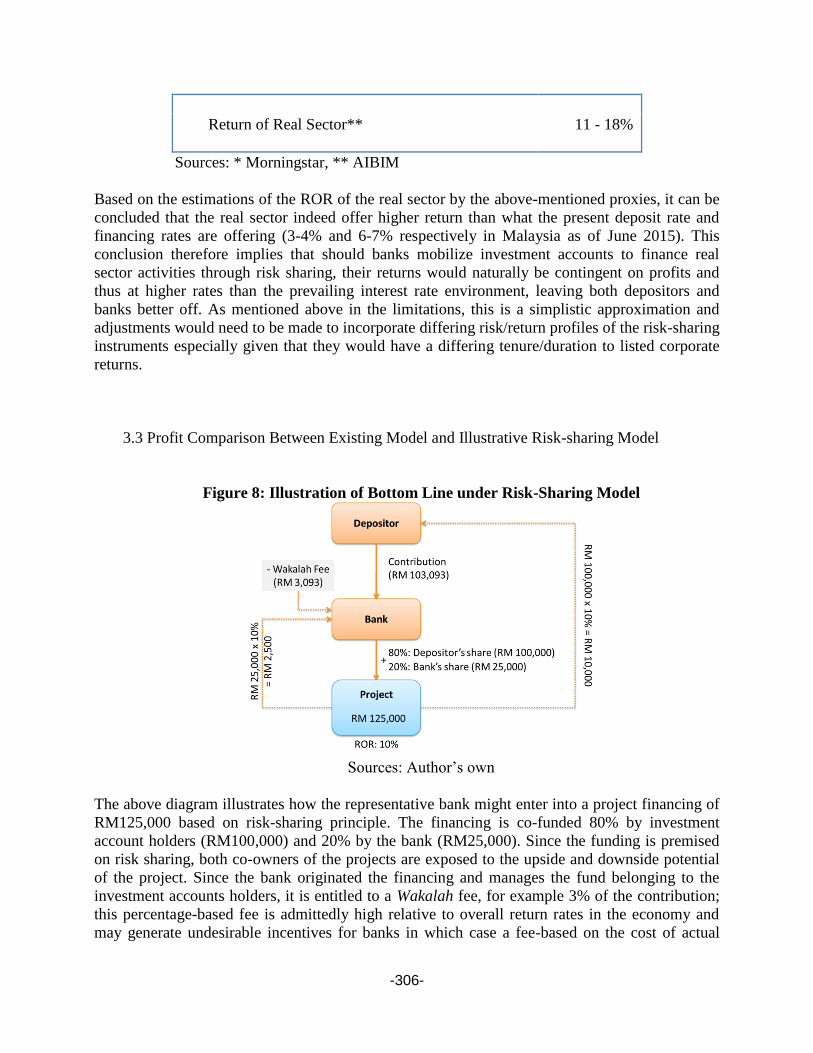
-306-

Return of Real Sector**

11 - 18%

Sources: * Morningstar, ** AIBIM

Based on the estimations of the ROR of the real sector by the above-mentioned proxies, it can be

concluded that the real sector indeed offer higher return than what the present deposit rate and

financing rates are offering (3-4% and 6-7% respectively in Malaysia as of June 2015). This

conclusion therefore implies that should banks mobilize investment accounts to finance real

sector activities through risk sharing, their returns would naturally be contingent on profits and

thus at higher rates than the prevailing interest rate environment, leaving both depositors and

banks better off. As mentioned above in the limitations, this is a simplistic approximation and

adjustments would need to be made to incorporate differing risk/return profiles of the risk-sharing

instruments especially given that they would have a differing tenure/duration to listed corporate

returns.

3.3 Profit Comparison Between Existing Model and Illustrative Risk-sharing Model

Figure 8: Illustration of Bottom Line under Risk-Sharing Model

Sources: Author’s own

The above diagram illustrates how the representative bank might enter into a project financing of

RM125,000 based on risk-sharing principle. The financing is co-funded 80% by investment

account holders (RM100,000) and 20% by the bank (RM25,000). Since the funding is premised

on risk sharing, both co-owners of the projects are exposed to the upside and downside potential

of the project. Since the bank originated the financing and manages the fund belonging to the

investment accounts holders, it is entitled to a Wakalah fee, for example 3% of the contribution;

this percentage-based fee is admittedly high relative to overall return rates in the economy and

may generate undesirable incentives for banks in which case a fee-based on the cost of actual

-307-

services undertaken may be more appropriate from the perspective of this paper which promotes

a model that incentivizes banks and their counterparts to undertake responsible risk-averse risk-

sharing behavior. The co-owners will receive the return of their respective investment on a

contingent ex-post basis from the project.

The following diagram compares the bank’s potential earnings derived under risk-transfer and

risk-sharing models. The results indicate that funders (investment account holders) have the

potential to earn significantly higher returns by investing via risk sharing than through depositing.

Meanwhile the bank has the opportunity to enjoy higher returns given the fee income and

enhanced real sector-linked returns (not OPR linked). The higher returns represent the upside

potential that entrepreneurs share with the investors in return for the financing of the business.

The detailed balance sheets of both banking model are provided in the Appendix.

Figure 9: Banks’ Margins: Risk Transfer vs risk Sharing Banking Models

As mentioned, this illustration is simplistic in nature given the limited scope of this paper. Further

research would need to adjust for the different risk-sharing asset classes and their respective

risk/return/maturity profiles, as well as for leverage in the real economy, to derive a more realistic

estimation. Additional considerations would be extra costs in the banking sector due to the

transition requiring an increased competency/skill level in bank officers as well as modeling

possible “default” rates. Also consideration needs to be given to cost savings from employing

Fintech and from reduced externalities (including regulation and capital buffers, deposit

insurance, legal documentation etc).

4. STRESS TESTING

Stress testing was originally used at the portfolio level, to understand and quantify the risks to a

trading book as a result of extreme movements in market prices. It is a form of simulation

technique used to shock the asset and liability portfolios to assess their reactions to changing

situations. In its simplest form, stress testing is a method to gauge how certain stressors will

affect a company or industry. For an individual entity, stress tests help to formulate business

-308-

strategy and planning, for capital management, and to set risk appetite and limits. Over time, its

scope of usage expanded from a risk management tool for a company to an early warning system

for the policymakers in detecting potential vulnerabilities of an entire financial system or an

economy to shocks (Jones, Hilbers and Slack, 2004).

In the context of this paper, a micro stress-testing technique is applied to test the sensitivity of

risk-sharing banking model vis-à-vis the risk-transfer model in response to asset price volatility

(i.e. ROR for risk sharing and overnight policy rate (OPR) for risk-transfer banking model).

Hypothetically, we assume that sudden volatility in the OPR for the risk-transfer system and the

ROR of the risk-sharing system would adversely impact the profitability of the banks. Trigger

factors for funding cost volatility in the risk-transfer system are mainly due to monetary or fiscal

policy decisions such as interest rate targeting, inflation targeting, exchange rate targeting or

macroeconomic purposes.

In the case of Malaysia and most economies, a change in OPR has a direct impact on the

financing rate of Islamic banks thus influencing their profit margin, even though banks’

profitabilities are largely based on asset quality and net interest margin (negating the effect of the

OPR). On the other hand, for the risk-sharing model, the OPR is no longer relevant as the

[unlevered] ROR of real sector determines the bank’s profitability together with value-added fee

income. In this case, different trigger factors would influence the ROR volatility such as

commodity/resource or stock market conditions, macroeconomic and political events, governance

and strategy or environmental and natural disasters. Depending on the severity of the events, the

change in ROR affects the cash flow of the projects being funded and returns to investors. The

most important difference between the two is in the source and application; as OPR is derived

from the financial sector and is ex-ante (and influencing profitability), while ROR is derived from

the real sector and is ex-post (derived from profitability).

Based on these assumptions, the stress test simulates three scenarios to estimate the potential

revenue declines triggered by changes in OPR for the risk-transfer model and ROR for the risk-

sharing model. To this end, a baseline, adverse and extreme scenarios are constructed for 2013

with both models being shocked to one, two and three standard deviations. The table below

shows the stress test result on the balance sheet of the current risk-transfer banking model.

Table 2: Depositor’s Return and Bank’s Margin: Current Model

MODEL

CURRENT MODEL (Risk Transfer)

RISK39 (%)

1.76 3.52 5.28

RISK ADJUSTED FINANCING

RATE (%) 5.29 5.19 5.10

39 represents the OPR volatility.

-309-

Baseline Adverse Extreme

DEPOSITOR'S RETURN (RM)

83,118,891 583,118,891 583,118,891

Change in RM

- -

Change in %

- -

BANK'S MARGIN (RM)

378,777,437 361,544,766 344,312,096

Change in RM

(17,232,670) (34,465,341)

Change in %

(4.5%) (9.1%)

Deposit rates are fixed under each scenario. There are two reasons for this treatment: (i) to reflect

the risk-transfer principle in the present model where risk and reward are not directly linked and

the management of liabilities (SIA and GIA) is separated from the management of assets

(financing), and (ii) the pre-IFSA practice of Islamic co-mingling investment accounts with other

types of savings where Islamic banks often limited the exposure of depositors to rate changes to

remain competitive to conventional banks, a form of displaced commercial risk, hence Islamic

banks in Malaysia utilized profit equalization reserve (PER) mechanisms. The following diagram

illustrates the stress test result on depositor and bank’s revenues under risk-transfer model.

The stress test on the risk-transfer model shows that the bank’s margin could decline by 5% or

RM17 million when the volatility is doubled and a decline of 9% or RM34 million when the

volatility is tripled. Indeed this can be translated into a significant risk to Islamic banks operating

in a low financing rate environment. For instance, banks’ margins could be negatively impacted

(and ultimately earnings) if the central bank decides to cut the OPR as financing rates will be re-

priced downward more than deposit rate.

Furthermore, the profit margin of our representative bank shows a downward trend over the

period under study (from 3.76% in 2009 to 2.04% in 2013). A prolonged narrowing of profit

margin could pose as a threat to the sustainability of Islamic banks. This in turn could have a

reputational impact on the industry that has gained recognition as a mainstream mode of finance.

Table 3: Representative Banks’ Margins in % for Period 2009 - 2013

YEAR 2009 2010 2011 2012 2013

REPRESENTATIVE

BANK'S MARGIN (%)40 3.76 2.99 2.73 2.38 2.04


40 Calculated as bank’s margin divided by the total financing

-310-

A similar trend has been observed by a study by Abdul Kader Malim et al. (2014) on the profit

margins of Islamic banks in the OIC countries for period 2005 to 2011. As indicated in the table

below, their study found that the average profit margin of Islamic banks in OIC countries has

been decreasing (from 4.14% in 2006 to 3.74% in 2011). Interestingly, the study also noted that

in comparison with the OIC average, Islamic banks in Malaysia experienced a consistently lower

profit margin throughout the period of study i.e. 3.16% in 2005 (OIC average: 3.90%) and 2.95%

in 2011 (OIC average: 3.74%). This perhaps indicates the more stable, mature and competitive

banking environment in Malaysia.

Table 4: Islamic Banks’ Margins (%) in OIC Countries and Malaysia

2005 2006 2007 2008 2009 2010 2011

Margins in

OIC Countries 3.90 4.14 4.21 4.10 4.20 3.74 3.74

Margins in

Malaysia 3.16 3.08 3.31 3.12 3.32 3.19 2.95

Source: Abdul Kader Malim et al., 2013

Under the risk-transfer operating model, Basel capital requirements are necessary to ensure

Islamic banks have sufficient buffers to absorb any sudden volatility. In such debt-based system,

studies argue that the greater proportion of debt tends to make banks more vulnerable to losses,

given that debt capital has lower loss absorbency capacity than equity.41 Such eventuality could

be avoided if Islamic banks fully employ a risk-sharing banking model that offers straight pass-

through and in-built loss absorbing and profit accreting mechanism.

The following paragraphs discuss the micro stress test conducted on the balance sheet of risk-

sharing banking model. To this end, the earlier estimated ROR of 20.98% was treated as the

baseline and was shocked at 2 and 3 standard deviations. As the bank is operating under risk-

sharing principle, investment account holders would be exposed to any adverse impact of

volatility. Since the investment account is a pass-through risk-bearing instrument, depositors fully

absorb the impact of ROR declines and benefit from upsides as well. Compared with the current

model where the bank absorbs the impact of volatility, the risk-sharing model spreads the impact

amongst the investors thus upholding the risk-reward principle.

In both the adverse and extreme scenarios, the test results suggested that bank profitability is less

sensitive to shocks than in the risk-sharing model with greater resilience. At 2 standard deviation

the risk-sharing bank’s profit declined by only 0.6% whereas the current model declined by 5%.

At 3 standard deviation the profit margin declined by 1.3% compared to the current model which

was far more exposed to a 9% decline. In short, the above micro stress tests suggested that in the

event of adverse situations, risk-sharing model is more stable than risk-transfer model.

41 IMF FSAP 2014 Stress Test on Malaysia, p. 15

-311-

Table 5: Depositor’s Return and Bank’s Margin of Risk-Sharing Model

MODEL

RISK-SHARING MODEL (ROR 20.98%)

RISK (%)

1.00

2.00

3.00

RISK ADJUSTED ROR (%)

20.77 20.56 20.35

Baseline Adverse Extreme

DEPOSITOR'S PROFIT (RM)

3,736,064,424 3,698,326,399 3,660,588,375

Change in RM

(37,738,024)

(75,476,049)

Change in %

(1.0%)

(2.0%)

BANK'S PROFIT (RM)

1,490,334,217

1,480,899,711

1,471,465,204

Change in RM

(9,434,506)

(18,869,012)

Change in %

(0.6%)

(1.3%)

Note: Depositor’s profit is derived from 80% contribution of total financing. Bank’s profit

is derived from 20% own contribution and 3% Wakalah fee

Based on the above micro stress testing, the risk-sharing model offers advantages over the present

risk-transfer model with a balance sheet that is less fragile owing to the matched assets and

liabilities structure and the one-to-one tagging of the assets to the real economic project/activities.

It saves the banks in terms of capital allocation on assets that are at risk, which the bank would

otherwise have to provide under the present model. In terms of fragility, the stress test illustrates

that the risk-transfer model is more fragile as it performs worse than risk-sharing in adverse

situation. The finding concurs with Calomiris and Haber (2014) that the present banking system

is indeed fragile by design.

From the government’s perspective, the risk-sharing banking model has a more far-reaching

agenda in inducing financial inclusion and creating incentive for asset building for low and

middle income groups in the society. Furthermore, it requires no deposit insurance and lender-of-

last-resort facility. These safety net mechanisms create unintended moral hazard for banks to over

leverage and lose rigor in selecting high quality funding opportunities. The risk-sharing model

also addresses the adverse selection and moral hazard issues, through the ‘skin-in-the-game’

requirement proposed by industry participants where banks need to co-own a percentage of

securities issued for investment projects. In this study, the banks are proposed to fund and retain

20% of the total value of each project financed.

5. CONCLUSION

Investigation on balance sheets confirms the “lend long and borrow short” practice of Islamic

banks in Malaysia. This exemplifies Islamic banks’ practice of replicating and conforming to the

-312-

typical business model of conventional banks. The investigation also noted the high concentration

of household financing (housing/mortgage, vehicle, credit card and personal financing). The

positive incentives created for risk-sharing finance via IFSA, recent BNM guidelines for

example, ring-fencing investment account and IAP have yet to make an impact in the industry. At

the time of writing in October 2015, BNM is in the process of issuing policy documents that

would ensure Islamic financial transactions truly reflect risk-sharing principles in line with Kuala

Lumpur and Jeddah declarations.

The investigation also illustrates the balance sheet structure based on matched assets and

liabilities. Such a structure offers greater stability and it firmly anchors the banking sector to the

real economy in line with risk-sharing principles. It involves real-sector tagging (materiality) and

one-to-one asset-liability matching in terms of value, risk and maturity. It promotes financial

inclusion as the members of public can own low denomination tradable securities. Returns on

these securities are derived ex-post from the actual performance of the underlying project. Under

the current post GFC suppressed rate environment, this implies that Islamic banks and investors

could realize additional revenues from the risk-taking model. Under this model, Islamic banks are

better off performing active investment intermediation on a risk-sharing mode rather than merely

operating substantively as borrowers and lenders. Islamic banks also would no longer faced with

liquidity, market and credit risks. Challenges can be addressed by the “skin-in-the-game”

requirement where banks co-own projects funded by the investment account holders of the banks,

as is the best practice in the securitization industry.

The risk-sharing banking model operates on an asset-driven balance sheet management thereby

ensuring that the financial sector grows in tandem with the economy, not creating bubbles (as it

did in pre the GFC) or hold back growth (as it has in the post GFC). It eliminates financial

oppression/repression and predatory lending as compensations to investors are determined by the

actual performance of the real economic activities. This ensures prosperity is shared equitably

amongst those who share the risks of any economic venture.

The micro stress test on the balance sheets also illustrate that risk-sharing banking is more

resilient to rate shocks than its risk-transfer counterpart. In adverse scenarios, risk-sharing model

exhibited a much lesser impact to the bank’s margin owing to the pass-through mechanism. It

also creates the incentive for Islamic banks from becoming over reliant on inflexible debt

contracts (Mian and Sufi, 2014). Risk sharing also reduces operating cost to the bank in terms of

the capital allocation on assets that are at risk, which the bank would otherwise have to provide

under the present model.

The model however is an illustrative first step undertaken under certain time and resource

constraints and as such suffers from some major limitations including, inter alia:

i. the unavailability of data for the ROR of the real sector;

ii. no estimate or adjustment was made for any leverage-based effects on the illustrative

estimated ROR;

iii. no estimate or adjustment was made for differing risk and maturity profiles that would be

present under the different asset tranches;

iv. no estimate or adjustment was made for any differential in “default” and recovery rates

between the two models; and, importantly,

-313-

v. no estimate or adjustment was made for any costs differentials in terms of transition to

and subsequent operation of a risk-sharing banking model, in terms of costs to banks (up-

skilling bank officers, cost savings from Fintech), bank customers (in terms of greater

alignment between funding and real activity) and externalities costs and savings.

Further research to explore the role of Fintech in furthering the advancement of Islamic finance is

necessary to ensure the risks and transaction costs of market participants could be kept minimal.

Fintech could potentially create value to the Islamic financial system such as in establishing

trusted investor-entrepreneur matching platform, seamless financing/investment selection and

funding processes, low-cost and efficient secondary markets for the trading of the risk-sharing

securities, and transparent real-time project monitoring mechanism.

REFERENCES

1. Abdul Latiff, R. & Halid, N. (2012). The Mudharabah Deposit Rate Behavior in Relation to

the Conventional Deposit Rate. Selangor: Journal of Management, National University of

Malaysia (UKM).

2. Abdul Kader Malim, N., Ibrahim, M., & Mohd Rasid, M.E.S. (2014), Financial

Intermediation Costs in Islamic Banks: Role of Bank-Specific, Market-Specific and

Institutional-Governance Factors, Islamic Banking and Finance Conference at Lancaster,

UK.

3. Admati, A. & Hellwig, M. (2013). The Bankers’ New Clothes: What's Wrong with Banking

and What to Do about It. New Jersey: Princeton University Press.

4. Ahmad, A. (2000). Instruments of Regulation and Control of Islamic Banks by the Central

Banks. Jeddah: Islamic Research and Training Institute.

5. Askari, H., Iqbal, Z., Krichene, N. & Mirakhor, A. (2012). Risk Sharing in Finance: The

Islamic Finance Alternative. Singapore: John Wiley & Sons.

6. Bacha, O. I. (2008). The Islamic Interbank Money Market and a Dual Banking System: The

Malaysia Experience, MRPA Paper 12699, University of Library of Munich, Germany,

Revised March 2008.

7. Bacha, O. I. & Mirakhor, A. (2015 – pending publication). A Risk Sharing Banking Model.

8. Bank Negara Malaysia (2007). Guideline on Stress Testing.

9. Bank Negara Malaysia (2015). Macro Stress Testing: The Approach in Malaysia.

10. Calomiris, C. & Haber, S. (2014). Fragile by Design. New Jersey: Princeton University Press.

11. Halid, N. & Abdul Latiff, R. (2012). Developing Reference Rate of Return Based on Real

Sector Economy: A Case for Malaysia. African Journal of Business Management, Vol. 6 (8)

pp. 2871-2877, 29 February 2012.

12. Jones, M., Hilbers, P. & Slack, G. (2004). Stress Testing Financial Systems: What To Do

When the Governors Calls. IMF Working Paper WP/04/127.

13. Mian, Atif & Sufi, A. (2014). House of Debt. Chicago: The University of Chicago Press.

14. Mirakhor, A. (2010). Whither Islamic Finance? Risk Sharing in an Age of Crises. Paper

presented at the Inaugural Securities Commission Malaysia (SC) – Oxford Centre of Islamic

-314-

Studies (OCIS) Roundtable “Developing a Scientific Methodology on Shariah Governance

for Positioning Islamic Finance Globally”, March 15, 2010, Kuala Lumpur.

15. Mirakhor, A. (2012). Shari’ah Compliant Macroeconomic Policy, 2nd ISRA Colloquium.

16. Mirakhor, A. (2014). Regulatory Framework for Islamic Finance. Islamic Banker Asia Issue

11.

17. Mohammed, N, Ismail, A. G., Muhammad J., Abdul Jalil S., Mohd Noor, Z. (2015). Market

Concentration of Malaysia’s Islamic Banking Industry. Jurnal Ekonomi Malaysia 49(1) 2015

pp.3-14. URL: http://dx.doi.org/10.17576/JEM-2015-4901-01

18. Omar, M.A., Md Noor, A. & Mydin Meera A. K. (2010). Islamic Pricing Benchmark. ISRA

Research Paper (No. 16 /2010)

19. Rosly, S. A. (2007). Islamic Banking: Doing Things Right and Doing Right Things.

Malaysian Journal of Economic Studies. June 6, 2007.

20. Rosly, S. A. & Ariff, M. (2011). Islamic Banking in Malaysia: Uncharted Waters. Asian

Economic Policy Review, Vol. 6, Issue 2, pp. 301-319

-315-

APPENDIX 1: BALANCE SHEET AND BANKS’ PROFIT: RISK-SHARING

MODEL

-316-

APPENDIX 2: BALANCE SHEET AND BANKS’ MARGIN: RISK-TRANSFER

-317-

APPENDIX 3: KUALA LUMPUR DECLARATION 2012

The Second Strategic Roundtable Discussion, jointly organized by the International Shari'ah

Research Academy for Islamic Finance (ISRA), the Islamic Research and Training Institute

(IRTI) and Durham University, met on 20th September 2012 in Lanai Kijang, Kuala Lumpur.

After lengthy deliberations on the issue of risk sharing, the participants acknowledged that

the financial crisis which started in 2008 highlighted the fact that the most salient feature of the

dominant conventional financial system is the transfer of risks away from financial institutions

onto customers, governments and the public at large. Islamic finance is in a unique position to

offer an alternative to the present interest-based debt financing regime that has brought the whole

world to the edge of collapse.

Bearing this in mind, the second annual ISRA-IRTI-Durham Strategic Roundtable

Discussion (2012) agreed on the following:

• The Shari’ah emphasizes risk sharing as a salient characteristic of Islamic financial

transactions. This is not only exemplified in equity-based contracts, like musharakah and

mudarabah, but even in exchange contracts, such as sales and leasing, whereby risk is shared

by virtue of possession.

• Risk transfer and risk shifting in exchange contracts violate the Shari’ah principle that liability

is inseparable from the right to profit.

• Sales must be genuine transactions in open markets.

• Although the Shari’ah recognizes the permissibility of debt, it is acknowledged that excessive

debt has detrimental effects on society.

The recommendations of the Roundtable Discussion are as follows:

1. Governments should endeavour to move away from interest-based systems towards enhancing

risk-sharing systems by levelling the playing field between equity and debt.

2. Accordingly, governments should increase their use of fiscal and monetary policies based on

risk sharing.

3. Governments could issue macro-market instruments that would provide their treasuries with a

significant source of non-interest-rate-based financing while promoting risk sharing, provided

that these securities meet three conditions: (i) they are of low denomination; (ii) are sold on

the retail market; and (iii) come with strong governance oversight.

4. There is a need to broaden the organizational structures beyond traditional banking models to

formats such as venture capital and waqfs to fulfil the social goals and risk-sharing features of

Islam finance.

Source: https://www.google.com/webhp?sourceid=chrome-

instant&ion=1&espv=2&ie=UTF-8#q=kuala+lumpur+declaration+2012+ISRA

-318-

EMPLOYEES OF STRESS LEVELS, THE EFFECT OF JOB SATISFACTION:

A FIELD STUDY

Adnan Çelik

Selcuk University, Turkey


Sadife Güngör


Email:[email protected]

Abstract

In this study, stress and the effects of these stresses on the academicians working in hospitals by

taking the opinions related with the stress and job satisfaction of the academicians working in the

health sector. Questionnaire method is used in the collection of the data. For the sampling of our

study, academicians targeted which make duty in different department of hospitals in Konya city

of Turkey. The number of the academic personnel working in hospitals is determined as

approximately 180 persons. Accordingly, this study shall be carried out over 180 persons, the

questionnaire number which is required to be made by considering the Sample Sizes ( α= 0.10)

table issued by Yazıcıoğlu ve Erdoğan (2004,) is determined as at least 93 with the sampling

failure of ± 0.05. As the result of the examination, 113 questionnaire forms have been obtained.

It is observed that the number of questionnaire which is obtained in this respect has the ability of

representing the universe. The data which is collected through the scale has been recorded to

SPSS 22.0 for Windows package program and the data has been analyzed. For variables, stress

and job satisfaction grades; Correlation, T test, F test, simple linear regression analyses were

made. The grade value of the five points Likert type items are collected in the questionnaires. The

significance level of the research has been taken as p<0,05. The findings which are obtained as

the result of the analysis have been commented by being converted into table in accordance with

the research questions. As the result; the academicians working in hospitals always face with the

stress in their professional lives. This decreases their job satisfaction. When the research- wide is

considered, a correlation (relation) in negative and high level is seen between the stress and job

satisfaction. No diversity of views is seen in whole demographic variables. In other words, their

opinions in stress and job satisfaction factors are in the same direction.

Keywords: Stress, Stress Management, Job Satisfaction, Academician

1. INTRODUCTION

The behaviors of the individual against the negative feelings are closely associated with the stress

concept. There both positive and negative effects of the stress. The positive results cause growth

and development; the negative effects cause depression and retreat (Güler, 2006: 10). The stress

word is the mixture of danger and opportunity words in Chinese. In the contrary of the wide

belief, the stress is not always bad. It may be an effective incentive which embellishes the life



-319-

(Rowshan, 2000: 12). The negative stress occurs under a few or too much tension. The positive

stress occurs in the cases where adequate tension is felt and a motivation is provided (Braham,

1998:46). Because successful persons turn their stresses into constructive energy and creative

power (Rowshan, 2000: 12). For example, an operator who makes operation in operation room is

so under pressure that his heart beats become so fast. They make a successful operation through

stress. A surgeon who is loose and is not under pressure during the operation, is not preferred by

anyone (Rowshan, 1998: 12).

In the first section of the study, the concepts and definitions related with the stress and works

satisfaction are analyzed, in second and third sections a research which is made on the academic

personnel in the hospitals working in health sector, is examined for determining the effect of the

stress on the work satisfaction, in the last section the findings which are obtained in the

questionnaire study, are tried to be evaluated.

2. CONCEPTUAL FRAMEWORK

The stress is a concept which is nearly confronted by everybody in daily life and professional

world. Today, stress is perceived as a serious problem which is qualified as the disease of the

modern community (Örücü and Demir, 1999: 59; Çelik, 2010: 229).

The stress concept originated from “Estrica” in Latin and from “Estrece” in old French. The

concept has been used in 17th century as disaster, trouble, misery, sadness and fatality (Pehlivan,

1995: 5). In 18th century, the meaning of the concept changed and was used for persons, objects

or spiritual structure in the meanings like stress, problem, pressure, power (Keser, 2014: 3). The

stress has been for identified by Canadian Physiologist Dr. Hans Selye in 1950. According to

Selye, stress is a general reaction given by the body against the pressures on it and he described

these reactions as “General Adaptation Syndrome (Selye, 1986; Şimşek and Çelik, 2008: 328).

Selye provided the wide usage of the stress as a science and discipline in the medical field today

with the work titled “Stress” (Ceyhan, 2012: 108). In other words, stress has been identified as

"physical and emotional reaction against the potential threats of the environment". This

identification shows the insufficiency of the harmony between the individual and environment

(Şimşek and Çelik, 2012:290). It is possible to gather the factors causing stress in two groups.

These are individual stress sources and organizational factors (Balcı, 2000: 10).

The individual, who fulfill specific roles and tasks in business environment, is confronted with

the "organizational stress" which arises from the organizational environment. This concept is also

expressed as the work stress or occupational stress (Pehlivan, 1995: 11). The work stress is an

issue which causes various costs for personnel and organization, effects the psychological and

physiological health of the employees (Şimşek and Çelik, 2008: 330). The work stress may be

caused by any reason in the organization. For example; the change in performing the work,

change in technology, handover of the establishment, merger with another establishment, tension

between the executive or colleagues of the individual may cause stress (Keser, 2014: 21). There

may be different stress sources affecting the employees in an organization. Some of these sources

may be listed as follows (Davis,1983: 442; Stoner and Fryer,1983: 34; Pehlivan, 2000: 26): The

excess workload, limitation of the time, tight and close audit, the insufficiency of the

authorization in meeting the responsibilities, insecurity of the political environment, uncertainty

of the role, disharmony between the values of the organization and individual, frustration, role

-320-

conflict, concern caused by the responsibilities, working conditions, human relations and

alienation.

The individual stress sources are; concern level, tolerance against the uncertainty, familial

problems, excite level, economic problems, disappointment, futility of the professional life and

the general changes in life (Çoşgun, 2006: 21).

The orientation of the employees in accordance with the objects of the organization and optimum

of the performance depends on providing satisfaction from their works in sufficient level. The

person deals with his work or activities related with the work in a mjor part of his life.

Accordingly, the satisfaction obtained from the work, becomes one of the important indications

in terms of the happiness of the person (Canik, 2010: 57).

The works have an important role in individuals' lives. The work satisfaction and significance

given to the work by the employee, is very important for efficient and effective performance of

the employee. There are many ways and methods for increasing the success and efficiency in the

organizations. One of the most important effective ways for taking successful and efficient

results in good and service production in the organization with bad working conditions is to

satisfy the employee in terms of material and non-material aspects (Şimşek and Çelik, 2008:

361).

If the state of mind occurring at the end of the work experience of the employee is positive, this is

identified as "work satisfaction", if the state of mind is negative, this is identified as "work

dissatisfaction" (Bedük, 2010: 108). In other words, the work satisfaction may be identified as

"the happiness which is provided by creating a work with the colleagues whom the employee

enjoys working together with and the material benefits gained from the work". If the employee

can see the presented work as perceptibly, this proud shall be a satisfaction source for the

employee. (Şimşek vd., 2015: 202). The work satisfaction identifies the level of satisfaction

which is felt due to the work and the significance and satisfaction level of the work (Çarıkcı,

2001: 162).

3. RESEARCH METHODOLOGY

The purpose of this research which is made in this section for measuring the relation between the

stress and work satisfaction of the academic personnel working in hospitals of Konya, shall

provide information about the hypothesis, object, method and findings of this research. The

results gained in the research shall be evaluated for whether being significance statistically and it

shall be examined whether the hypotheses are verified.

3.1. Method of the Research and Sample

The questionnaire method is used in the collection of the data of this research. For the sampling

of our study, academicians working in different departments of hospitals in Konya are targeted.

The questionnaire form consists of two section, in the first section, there are questions which aim

to determine the demographic specifications of the participants. In the second section, there are

questions which determine the opinions of the participants related with their stress and work

satisfaction. The questionnaire form has been taken from the annex of the non-published master

-321-

thesis of Coşgun (2006). This study shall be carried out over 180 persons and the number of

questionnaire which must be made by considering the samples size ( = 0.10) table issued by

Yazıcıoğlu and Erdoğan (2004), is determined as at least 93 with the sampling error of 0.05.

113 questionnaire forms are obtained at the result of the performed examination. It is observed

that the obtained questionnaire form number has the ability to represent the main mass.

3.2. Analyzing and Commenting the Data

The data which is collected through the scale has been recorded to SPSS 22.0 for Windows

packaged software and the data has been analyzed. For the variables and the stress and work

satisfaction points; correlation, t test, basic linear regression analyses have been made. The point

values of the five point Likert type items have been collected in questionnaires.

The lowest and highest point interval of the stress scale; 15-26 Strongly disagree, 27-38

Disagree, 39-50 Indecisive, 51-62 Agree, 63-75 Strongly Agree. The higher point interval leads

increase in stress experience level. The lowest and highest point interval of work satisfaction

scale; 5-7 Strongly disagree, 8-10 Disagree, 11-13 Indecisive, 14-16 Agree, 17-20 Strongly

Agree.

The higher point interval leads increase in stress experience level. The significance level of the

research has been taken as p<0,05. The findings which are obtained as the result of the analysis

have been commented by being converted into tables in accordance with the research questions.

3.3. Hypotheses of the Research

Hypothesis-1: The opinions of the academicians working in hospitals of Konya related with the

stress, affect the work satisfaction as significantly;


stress and work satisfaction, show significant distinctness according to their ages;


stress and work satisfaction, show significant distinctness according to their genders;


stress and work satisfaction, show significant distinctness according to their marital status;


stress and work satisfaction, show significant distinctness according to their education status;


stress and work satisfaction, show significant distinctness according to their service period.

4. FINDINGS OF THE RESEARCH

Table 1, relates to demographic information.

-322-

Table-1: Frequency Distribution Table of the Participants

Variables Frequency (f) Percentage (%)

Age

18-30 Years Old 44 38,9

31-40 Years Old 34 30,1

41 Years Old and Over 35 31,0

Gender

Female 57 50,4

Male 56 49,6

Marital Status

Married 83 73,5

Single 30 26,5

Education Status

Bachelor 30 26,5

Post-Graduate 31 27,4

Doctorate 52 46,0

Service Period

5-10 Years 39 34,5

11-20 Years 31 27,4

21 Years and Over 43 38,1

General Total 113 100 (%)

The research has been made on total 113 persons. % 38.9 of the ages of the participants are 18-30

years old, % 30,1 of the ages are 31-40 years old and 41 years old and over. The %50.4 of the

genders of the participants is female and % 49,6 is male. The % 73.5 of the marital status of the

participants is married and % 26,5 of the participants is single. The %26.5 of the participants is

bachelor, % 27,4 post-graduate and % 46,0 doctorate graduate. % 34.5 of the service periods of

the participants is between 5 and 10 years % 27,4 is between 11 and 20 years and % 38,1 is

between 21 years and over.

The regression analysis results related with prediction of stress for the work satisfaction, are

given in Table 2. R value represents the correlation between dependent variable and independent

variable. The highness of this value shows that there is a close relation between the independent

variable and dependent variable or the independent variable explains an important part of the

change in the dependent variable.

In Table 2, R is 906) and it expresses a relationship between dependent variable and independent

variable which may be considered as negative and important. R Square value expresses that the

variance of % 82 in dependent variable is explained by the independent variable.

Table-2: Simple Regression Analysis Results Related with Stress and Work Satisfaction

Variable B Standard

Erroe β t P Dual r Partial r

Stable 85,784 1,130 - 75,893 ,000 - -

Stress -2,671 ,118 -,906 -22,548 ,000 -,906 -,906

R= ,906* R2= ,821 F (1,111)= 508,415 p=,000

-323-

* Work satisfaction (Dependent variable) is stable

As seen in Table 2, is, 821. It means that % 82 of the variance in dependent variable may be

explained. With a simpler expression, to know the stress in predicting the work satisfaction

enables prediction with the % 82 certain degree. When the dual and partial correlations between

the predictor variables and dependent (predicted) variable, are examined; it is seen that there is a

negative and high level (r=-,91) relation between the stress and work satisfaction.

When t-test results related with the significance of regression coefficients are evaluated; it is

observed that the stress is a predictor on work satisfaction (significant). Under the light of all

these expression, the stress gives a negative, high level and significant relationship with the work

satisfaction points. Under the light of these findings “The opinions of the academicians working

in hospitals of Konya related with the stress, affect the work satisfaction as significantly…” is

supported. According to the regression analysis, the regression equality (mathematical model)

related with the prediction of stress and work satisfaction, is given as follows (Y= 85,784-

2,671.Stress).

The averages of academicians working in hospitals of Konya according to the age variable

related with the stress and work satisfaction are given in Table 3.

Table-3: Anova Table Results According to Age Variable

Dimensions Variable N

SS F P LSD

Work

satisfaction

18-30 Years old 44 9,16 3,93

,396 ,674 -

31-40 Years Old 34 8,85 3,50

41 Years Old and

Over 35 8,43 3,33

Total 113 8,84 3,60

Stress

18-30 Years old 44 60,27 11,43

1,182 ,311 -

31-40 Years Old 34 63,71 9,83

41 Years Old and

Over 35 63,06 10,26

Total 113 62,17 10,63

* The relation is significant in p<0,05 significance level

The opinions of the academicians show distinctions according to the averages and dimensions. In

addition to this, bilateral variance analysis (ANOVA) has been made for determining whether

these differences between the averages of the academicians in terms of age variable are

statistically significant. The significance level of the difference between the averages of the

academicians in terms of age variable are found in Table 3.

When the descriptive statistics are examined, the scale reference interval in stress for

academicians in all ages are as "agree" and "strongly agree". It is "disagree" in work satisfaction.

The academicians working in hospitals in Konya, express that they have dense stress and this

decreases their work satisfaction.

The age groups are in the same opinion in this issue. Under the lights of these findings

"Hypothesis 2: The opinions of the academicians working in hospitals of Konya related with the

-324-

stress and work satisfaction, show significant distinctness according to their ages" are rejected in

both dimensions.

The opinions related with stress and work satisfaction of the academicians working in the

hospitals in Konya, are grouped according to gender variable and "independent two groups t test"

is applied. T test results according to gender variable are given in Table 4.

Table-4: T Test Table Results According to Gender Variable


ss sd t p

Work

Satisfaction

Female 57 9,16 3,80 111 ,943 ,348

Male 56 8,52 3,40

Stress Female 57 61,68 10,97

111 ,487 ,627 Male 56 62,66 10,35

*The relation in p<0,05 significance level ,is significant

It is observed that the differences between the averages are not statistically significant. The

highness of the significance (p values) degrees of t values more than %5 shows the non-existence

of a significant difference related with this analysis. In a general expression, regardless of the

genders of the academicians, their opinions related with work satisfaction and stress are in the

same direction.

When the descriptive statistics are examined, the opinions of the male and females are "agree". In

another words, the academicians working in hospitals of Konya, experience stress in dense level

and this affects their work satisfactions negatively. However, regardless of their genders, their

opinions are in the same directions.

Under the lights of these findings "Hypothesis 3. The opinions of the academicians working in

hospitals of Konya related with the stress and work satisfaction, show significant distinctness

according to their genders" are rejected in both dimensions.

The opinions related with stress and work satisfaction of the academicians working in the

hospitals in Konya, are grouped according to marital status variable and "independent two groups

t test" is applied. T test results according to marital status variable are given in Table 5.

Table-5: T Test Table Results According to Marital Status Variable

Dimension Variable N

ss sd t p

Work

Satisfaction

Married 83 8,53 3,47 111 1,533 ,128

Single 30 9,70 3,90

Stress Married 83 62,77 10,53

111 1,003 ,318 Single 30 60,50 10,89

*The relation in p<0,05 significance level ,is significant

It is observed that the differences between the averages are not statistically significant. The

highness of the significance (p values) degrees of t values more than %5 shows the non-existence

of a significant difference related with this analysis. In a general expression, regardless of the

-325-

marital status of the academicians, their opinions related with work satisfaction and stress are in

the same direction.

When the descriptive statistics are examined, the opinions of the married persons and single

persons are "agree". In another words, the academicians working in hospitals of Konya,

experience stress in dense level and this affects their work satisfactions negatively. However,

regardless of their marital status, their opinions are in the same directions.



according to their marital status" are rejected in both dimensions.

The averages of academicians working in hospitals of Konya according to the education status

variable related with the stress and work satisfaction, are given in Table 6.

Table-6: Anova Table Results According to Education Status


SS F p LSD

Work

Satisfaction

Bachelor 30 7,87 2,94

2,519 ,085 - Post-Graduate 31 9,90 3,99

Doctorate 52 8,77 3,60

Total 113 8,84 3,60

Stress

Bachelor 30 64,37 9,90

1,134 ,326 - Post-Graduate 31 60,29 11,15

Doctorate 52 62,02 10,69

Total 113 62,17 10,63




these differences between the averages of the academicians in terms of education status variable

are statistically significant. The significance level of the difference between the averages of the

academicians in terms of education status variable are found in Table 6.


academicians in all education status is as "agree" and "strongly agree". It is "disagree" in work

satisfaction. The academicians working in hospitals in Konya, express that they have dense stress

and this decreases their work satisfaction. The education status groups are in the same opinion in

this issue.



according to their education status." are rejected in both dimensions.

The averages of academicians working in hospitals of Konya according to the Service period

variable related with the stress and work satisfaction are given in Table 7.

-326-

Table-7: Anova Table Results According to Service Period Variable

Dimension Variable N

SS F p LSD

Work

Satisfaction

5-10 Years 39 9,49 4,00

2,519 ,085 - 11-20 Years 31 8,48 3,48

21 Years and Over 43 8,51 3,30

Total 113 8,84 3,60

Stress

5-10 Years 39 60,15 11,73

1,134 ,326 - 11-20 Years 31 63,61 9,99

21 Years and Over 43 62,95 9,97

Total 113 62,17 10,63




these differences between the averages of the academicians in terms of service period variable are

statistically significant. The significance level of the difference between the averages of the

academicians in terms of service period status variable are found in Table 7.


academicians in all service period is as "agree" and "strongly agree". It is "disagree" in work

satisfaction. The academicians working in hospitals in Konya, express that they have dense stress

and this decreases their work satisfaction. The service period groups are in the same opinion in

this issue.



according to their service period." are rejected in both dimensions.

5. RESULTS

A research is made for the opinions of the academicians working in hospitals of Konya related

with the stress and work satisfaction and for measuring the stress of the academicians in hospitals

through a significant literature scanning and a comprehensive field research and for measuring

the effects of these stresses on the work satisfaction. When the descriptive statistics are

examined, it is observed that the academicians do not have time for their private lives, the current

legislation and bureaucratic obstacles affect their work lives negatively, non-existence of the

merit system and they express an opinion such as agree and strongly agree on the stress lives

arising from the non-existence of the notifications. On the other hand, they express that while

working, they take orders from many executives and chiefs, the night work and shifts bother

them. They express an opinion as disagree in the work satisfaction level due to this and similar

issues. When the analytic statistical results are examined, it is found that there is a negative and

-327-

high level relation between the stress and work satisfaction. We may say that when the stress

increases, the work satisfaction decreases and when the work satisfaction increases, the stress

decreases.

In the findings of this research, it is found that the stress reference intervals of the academicians

are stressful and they express agree and strongly agree to the points where they experience stress.

The works satisfactions are in the direction of agree and strongly agree in dissatisfy, have no

work satisfaction points. As the result of the basic linear regression analysis, it is found that %82

of the stress of the r square value is explained in the work satisfaction. A negative and high level

correlation is observed among them. In the analyses made related with the age, gender, marital

status, education status, service period, it is found that no diversity of views are observed in any

of these variables.

As the result, the academicians working in the hospital are confronting with the stress in their

work lives. This increases their work satisfaction. When the generality of the research is

considered, a negative and high level correlation (relation) is observed between the stress and

work satisfaction. No opinion differences are seen in all demographic variables. In other words,

their opinions in stress and work satisfaction factors are in the same direction.

References

1. Balcı, Ali (2000), Öğretim Elemanının İş stresi Kuram ve Uygulama, Nobel yayın,

Ankara.

2. Bedük, Aykut (2010), Karşılaştırmalı İşletme Yönetim Terimler Sözlüğü, 3.Baskı,

Atlas Kitabevi, Konya.

3. Braham, Barbara J. (1998), Stres Yönetim”, Çev. Vedat G. Diker, Hayat Yayıncılık,

İstanbul.

4. Canik, Burcu (2010), “Esenboğa Havalimanında Farklı Birimlerde Çalışanların Stres

Düzeylerinin İş Tatmini Üzerine Etkisi”, Yüksek Lisans Tezi, Gazi Üniversitesi,

Sosyal Bilimler Enstitüsü, Ankara.

5. Ceyhan, Bilal (2012), “Örgütsel Stres Yönetimi ve Stresin İstanbul Büyükşehir

Belediyesi Çalışanlarının İş Performansı Üzerine Etkisinin Uygulamalı Olarak

İncelenmesi”, Yüksek Lisans Tezi, Bahçeşehir Üniversitesi, Sosyal Bilimler Enstitüsü,

İstanbul.

6. Coşgun, Nükhet (2006), “Çalışma Hayatında Stres ve İyimserliğin İş Tatminine Etkisi

ve Bir Araştırma”, Yüksek Lisans Tezi, İstanbul Üniversitesi, Sosyal Bilimler

Enstitüsü, İstanbul.

7. Çelik, Adnan (2010), “Kriz ve Stres Yönetimi, Gazi Kitabevi, Ankara.

8. Çarıkçı, İlker (2001), “Çalışanların İş tatminini Etkileyen Kişisel Özelikler ve

Örgütsel Sonuçları”, Milli Prodüktivite Merkezi Verimlilik Dergisi, s.161-178.

9. Güler, Burcu K. (2006), Çalışma Hayatında Öğrenilmiş Çaresizlik, Liberte Yayınları,

Ankara.

-328-

10. Keser, Aşkın (2014), İş Stresi Kaynakları: Geleneksel ve Güncel Boyutlarıyla, Ekin

Yayıncılık, Bursa.

11. Pehlivan, İnayet (1995), Yönetimde Stres Kaynakları, Pegem Yayınları, Ankara.

12. Pehlivan, İnayet (2000), İş Yaşamında Stres, Pegem Yayınları, Ankara.

13. Rowshan, Arthur (1998), Stres Yönetimi, Çev. Şahin Cüceloğlu, Sistem Yayıncılık,

İstanbul.

14. Rowshan, Arthur (2000), Stres Yönetimi, 2.Baskı, Çev. Şahin Cüceloğlu, Sistem

Yayıncılık, İstanbul.

15. Şimşek, M. Şerif ve Adnan Çelik (2008), Çağdaş Yönetim ve Örgütsel Başarım,

Eğitim Kitabevi, Konya.

16. Şimşek, M. Şerif ve Adnan Çelik (2012), Yönetim ve Organizasyon, 12.Baskı, Eğitim

Kitabevi, Konya.

17. Şimşek, M. Şerif ve diğerleri (2015), Davranış Bilimlerine Giriş ve Örgütlerde

Davranış, 9.Baskı, Eğitim Kitabevi, Konya.

-329-

THE EFFECT OF ETHICAL CLIMATE PERCEPTION OF TEACHERS TO THEIR

ORGANIZATIONAL COMMITMENT: A SAMPLE PRACTICE

Adnan Çelik



Emine Et Oltulu



Beyhan Ozgu Cakir

KTO Karatay University, Turkey


Abstract

Nowadays, organizations are making an effort to minimize the problems that could affect

productivity and performance by doing research on human behaviours. To investigate and

analyse ethical climate and organizational commitment, which is the subject of the study, are

important in terms of contribution of the organizations to this development. With the increase of

competition in businesses, each factor of the organization has been required to be handled in a

more detailed way. In particular, the human factor has become the key point of the success. A

high ethical climate and high level organizational commitment is required also for those who

work in education sector to increase their success and performance in the institutions they work.

In this study, teachers’ perception of ethical climate on organizational commitment was

investigated. The sample of the research is consisted of the teachers who work in primary and

high schools of 5 districts of Konya. 337 teachers from different schools participated in this study

and a survey of 67 questions were applied to the participants. Obtained data analysed, tabulated

and interpreted through statistical programs.

Keywords: Ethical Climate, Organizational Commitment.

1. INTRODUCTION

In today’s business world where competition increasingly continues, the pace of the change fact

has reached incredible dimensions. The priority target of the enterprises operating in this

environment has been to be successful in global competition and maintain their existence in this

way. This can only be realized with the businesses being aware of the characteristics that make

them different from their competitors. At this point, the human factor has an undeniably great

importance.

Ethical climate and organizational commitment, which is part of the organizational culture, also

has an importance for schools. Especially the ethical climate practices which has a different place

to determine the ways that can be applied in the solution of problems that include ethical

practices provide power, confidence and role flexibility. The organizational commitment of

employees is the effort put forth to achieve the organization/operation’s goals and loyalty to the




-330-

organization. Thus, the role of organizational commitment is important to direct the employees to

a purpose within the framework of organizational culture.

In this study, teachers’ perception of ethical climate on organizational commitment was

investigated. Primarily, the concepts of ethical climate and organizational commitment were

emphasised. Following, the data which was obtained by applying a methodology intended for the

reliability studies of the ethical climate and organizational commitment behaviour scale created

by combining two separate studies analyzed and investigated through SPSS programme. The

main purpose of this study is to determine the effect of the perception of the ethical climate of

teachers on organizational commitment. For this purpose, the scales, developed to investigate

ethical climate and organizational commitment behaviour on 337 primary and high school

teachers who work in five different districts that selected from the province of Konya, were used.

In the study, ethical climate principles were approached with egoism and helpfulness dimensions.

Organizational commitment was approached with emotional dimension, rational dimension and

normative dimension. In result part of the study, the analyzes and results conducted on the data

collected within investigation were explained in a detailed way and the obtained results in

relation to performed analyzes were investigated. As a result, a meaningful and positive

relationship was found between ethical climate and organizational commitment.

2. ETHICAL CLIMATE

2.1. Ethics and Climate Concepts

Ethics, whose emergence almost extends to the early days of history of humanity when evaluated

on the basis of moral concept, is a concept that basically exists in the society all the time and

questioned within the life. Especially, in recent years, it has been a concept that is mentioned and

argued about it by every discipline. Nowadays, too, it became substantially questioned and

investigated globally (Sabuncuoğlu, 2011: 1).

If the concept of ethics is explained; the word ethics comes from Greek and derives from the

word ‘ethos’ which means ‘character’. The concept of ‘ethics’ which derives from ethos , too,

comes out with the investigation of moral principles and values by emphasising on ideal and

abstract one. In this respect, ethics is more specific and philosophical based than common moral

principles (Fromm, 1995: Yörükhan, 2015). As well as being reference values , principles and

standards for people to determine how things should be done , ethics, at the same time , is a

process and while taking a decision and applying in this process, actions should be taken by

adhering to certain values (Sabuncuoğlu, 2011:2).

The concept of climate is originally a Greek word and means ‘inclination’, ‘tendency’. Besides, it

is used to express physical phenomenon’s like heat, pressure and temperature. With its meaning

in business literature, it expresses how ‘climate’ business members evaluates the internal and

external environment of the organization (Haller, 1971:27; Büte, 2011: 172).

2.2. Ethical Climate

The concept of ethical climate which initially developed by Victor and Cullen (1988), serves

many functions in the organizations. When ethical dilemmas occur in solving ethical problems of

the individuals, the individuals in the organization seek an answer to question ‘what should I do’.

-331-

Another function of it is to determine ethical problems of the individuals in the organization; in

short, it is useful for diagnosing and evaluating the conditions of ethical climate individuals

(Cullen, Victor and Parboteeah, 2003: 129).

Ethical climate takes an active role in evaluating the incidents the employees’ faces in any

situation and determining what is right and wrong. In this sense ethical climate is one of the

important factors of organizational performance that shapes inter-organizational relationships and

attitudes of workers. Therefore, it is very important to understand possible relationship between

ethical climate of the organization and the attitudes of the workers (Elçi and Alpkan 2009: 299;

Karadut, 2014: 12).

Ethical climate of an organization is consisted of established norms and applications that function

as borders of what is right or wrong morally in the organizational context (Özgener, 2004;

Tütüncü and Savran, 2007: 179-180). When faced with a decision-making situations which is

important for other individuals in the organization, how an organization member should define

the ‘right’ alternative, at least the one suitable to the organization’s point of view? This

information constitutes work climate and determines the formation of ethical behaviours on the

work (Sağnak, 2005: 38; Tütüncü and Savran, 2007: 179-180).

The ethics concept in enterprises has become an intense need since the times modern businesses

emerged and are accepted as discipline. Especially within modern-day business world where

borders were removed commercially speaking, this interest has become intense. When considered

the existence of the subjects that can be associated with ethics everywhere human exists, the

enterprises which try to achieve their basis goals like profitability, sustainability and growth

within the brutal competition environment started to question ethics and pursue their activities

accordingly (Sabuncuoğlu, 2011: 29-30).

2.3. Ethics Climate Types

Three ethical approaches comprise the basis of ethical climate models in the leadership of Victor

and Cullen. These approaches cover the ethical basis of egoism, helpfulness and principlism. The

first approach is egoism. Egoism represents the organizational behaviour for both individual and

organization that is in search of escaping from the punishment and rewarding. This often causes a

climate where individual and organizational activity and cost activities are the primary target in

terms of productivity. The second approach is helpfulness. This approach represents the

behaviour that investigates employment in satisfactory good conditions for the members and that

allows it. The main element of this approach is its being functional and democratic (Mill 2002;

Akkoç, 2012: 47).

The helpfulness approach targets friendship, interpersonal relationship and encouragement to

group commitment. . In this context, the third is principlism. This approach focuses on abstract,

impersonal behaviour rules of conduct rather than individual or group satisfaction. When faced

with an ethical dilemma organization norms suggest to be adhered to rules or standards in the

decisions taken by the employees (Victor and Cullen, 1988; Akkoç, 2012: 47)

-332-

2.4. Ethical Climate Dimensions

Ethical climate of a company was actually defined, by theoretically grounding and after

experimental researches, in the context of five dimensions as due diligence, law and codes, rules,

benefit and independence. The due diligence dimension of ethical climate is related to the care to

the employees, company and against the world. Law dimension is related to rules of conduct

completely determined by the world. Rules dimension is related to rules of conduct accepted by

the company. Benefit dimension covers the rules enacted by individuals’ personal interest and the

enterprise. Independence dimension is related to personal rules of an individual within acceptable

behaviours (Neubaum, Mitchell and Schminke; 2004: 335-347; Tütüncü and Savran, 2007: 181-

182).

3. ORGANIZATIONAL COMMITMENT

3.1. Conceptually Organizational Commitment

In his theory, Philosopher Adams, suggest that employees should squarely be appreciated and

rewarded to be able to work with the high level of moral and motivation, to increase commitment

of them to the organization, and to have a trust in the organization and superiors (Eren, 2014:

551).

Organizational commitment was explained by focusing on generally three subjects defined as a

multidimensional concept. These are emotional commitment, continuity commitment and

normative commitment (Sabuncuoğlu, Tüz, 2013: 70).

According to another definition, organizational commitment is defined as organization employees

to believe, to adapt the objectives and values of the organization, to put an effort for

organizational goals, to have a strong desire to stay in the organization (Bedük, 2012: 179).

3.2. Dimensions of Organizational Commitment

According to Allen and Meyer is a psychological state that connects individual to the

organization. It is examined in three dimensions. These are emotional commitment, normative

commitment and rational commitment (Bedük, 2012: 179).

3.2.1. Emotional Commitment

Behavioural commitment is based on socio-psychological perspective. It is related to past

experiences of the individuals and process of dependency of them to the organization based on

the adaptation state to the organization (Clifford, 1989: 144). According to Meyer and Allen

behavioural commitment is a concept related to the issue of individuals to work too long in a

certain organization and how they dealt with this issue. According to these authors, employees

who show behavioural commitment are adhered to certain activities they do rather than the

organization itself (Meyer and Allen, 1997; Çöl, 2015).

-333-

Emotional commitment is that employees connect to the organization emotionally; continuity

commitment is that the employees connect to the organization by considering the cost of leaving

the organization (Sabuncuoğlu and Tüz, 2013: 70).

Emotional commitment covers the emotional commitment of the wage earner to the organization,

identification and integration of him/her with the organization. The wage earners who stays in the

organization with a strong emotional commitment stay on the organization not because they need

this, but they want this more themselves. (Meyer and Allen, 1991: 67; Doğan and Kılıç, 2015:

44).

3.2.2. Normative Commitment

Normative commitment is expressed as the employees feels connected to the organization as they

have a sense of moral duty and a belief not to leave the organization (Meyer and Allen, 1997;

Özdevecioğlu, 2003: 114). It is the commitment of the employee to the organization by feeling

the obligation of staying in the organization (Sabuncuoğlu and Tüz, 2013:70).

3.2.3. Rational Commitment

It is a commitment that occurs with the feeling of losing the gains wage earner got as a result of

the sacrifice within the work time in the organization after leaving the organization. It is

continuing to work of individuals in an organization because of obligation.

3.3. Factors Affecting Organizational Commitment

3.3.1. Personal Factors

It can be examined under the heading of job expectations, psychological

contract, personal characteristics in itself (Karasoy, 2014: 64-65).

3.3.2. Organizational Factors

There are many factors that enter into the scope of organizational factors. Some of them are the

quality of work and its importance, management, wage level, organizational culture,

organizational justice, organizational rewards, teamwork and career (Karasoy, 2014: 64-65).

3.3.3. Out of Organizational Factors

New job opportunities, professionalism, unemployment rate, the country's socio-economic status,

the state of the industry (Karasoy, 2014: 64-65).

-334-

3.4. Organizational Commitment Results

The results of commitment to the organization can be positive or negative related to the degree of

commitment. When organizational goals are not acceptable, the high degree of commitment of

the members can accelerate the separation of the organization; when the goals are reasonable and

acceptable, high degree of commitment is possible to result with effective behaviours. As regards

to the results of organizational commitment, it is found that behavioural results are in the

strongest connection with commitment. Of these, especially, job satisfaction, motivation,

participation and desire to remain in the organization have a positive relationship with

organizational commitment; job change and absenteeism have a negative relationship with

organizational commitment (Balay, 2000: 45).

4. SAMPLE PRACTICE

4.1 Research Methodology

4.1.1. Research Objective

Objective of this research is to measure the effects of teacher’s ethical climate on their

organizational commitment.

4.1.2. Data Collection Process

Research samples are elementary and high school teachers who work in five different counties of

Konya (Derbent, Hüyük, Yunak, Derebucak, Doğanhisar). Survey was used as a data collection

tool, and 337 questionnaires were administered. The questionnaire used in the study consists of

three sections.

4.1.3. Analysis Method

In the first section, 6 questions were asked about demographic characteristics of teachers (gender,

marital status, education level, age range, work duration and branches).

In the second section, questions about measuring organizational commitment were asked. With

this goal, 25-question organizational commitment survey which was quoted from Allen and

Meyer’s (1990) “The Measurement and Antecedent of Effective, Continuance and Normative

Commitment to the Organization” articles. Turkish version of this scale was taken from İbrahim

Cem Gültekin’s (2004) “The Relationship between Organizational Commitment and Job

Satisfaction” master thesis. The validity and reliability of the scale was checked by Gideon

(Gültekin, 2004; Eser, 2007: 42). Employees were requested to mark relevant choices such as

“Strongly Agree”, “Quite Agree”, “Somewhat Agree”, “Barely Agree”, and “Disagree” in the

second part of the survey.

In the third section, a 36-statement scale which was suggested by Victor and Cullen (1993) and

accepted as the most widely-used in order to specify ethical climate in the literature was used.

-335-

Turkish version of this scale was quoted from Eser’s (2007) master’s thesis named “Ethical

Climate and Effects of Trust in Manager on Organizational Commitment”. The validity and

reliability of the scale was checked by Eser. Organizational communication questionnaire was

developed as a result of literature review. Questionnaire participants were requested to mark the

questions based on 5-Likert-type scale as “Strongly Agree”, “Quite Agree”, “Somewhat Agree”,

“Barely Agree”, and “Disagree”.

4.1.4. Research Hypothesis

Hypothesis 1: There is a significant and positive correlation between ethical climate and

organizational commitment.

Hypothesis 2: There is a significant and positive correlation between Egoist Climate Type and

Emotional Dimension of Organizational Commitment.

Hypothesis 3: There is a significant and positive correlation between the Emotional Subscale of

Organizational Commitment and 3 dimensions (Egoist, Helpfulness and Principlism) of Ethical

Climate.

Hypothesis 4: There is a significant and positive correlation between the Continuation Subscale

of Organizational Commitment and 3 dimensions (Egoist, Helpfulness and Principlism) of

Ethical Climate.

Hypothesis 5: There is a significant and positive correlation between the Normative Subscale of

Organizational Commitment and 3 dimensions (Egoist, Helpfulness and Principlism) of Ethical

Climate.

Hypothesis 6: Is there a difference between the individual working times according to

Organizational Commitment, Ethical Climate and Sub-dimensions scales?

4.2. Research Method

Material design: In this research, statistical studies, and statistical analysis and review software

package SPSS 15 was used. In general, frequency and average based on the data were provided.

After this data was given, in order to decide on which type of tests to use for them, compliance

with the normal distribution of the data was tested with Kolmogorov-Smirnov normality test. As

a result of data normality and homogeneous heteroscedasticity, Parametric Tests will be

consulted; otherwise non-parametric tests will be used. In case of normal distribution of data and

uniform compliance is with variance, independent samples t test and one-way analysis of

variance of the parametric tests (ANOVA) test will be used. Here, when the number of groups

was two, two independent sample t test of parametric tests was used and when the number of

groups is more than two and they are independent groups, ANOVA test was used, and for the

correlation Pearson Correlation coefficient was used. Also, while finding out the mediating

variable, Structural Equation Modelling and Sobel test were used.

-336-

4.3. Demographic Characteristics

Table 1: Gender Frequencies

Tab

le 2:

Mari

tal

Status Frequencies

Tab

le 3:

Age

rang

e of frequencies

4.4. Analysis of Hypothesis

Hypothesis 1: There is a significant and positive correlation between Ethics Climate and

Organizational Commitment.

Organizational Commitment

Ethical Climate r=0,502

P value= 0,000

Pearson Correlation Test was made for the correlation between Ethical Climate and

Organizational Commitment trust and as the P value is equal to 0,000<0,05, there is a meaningful

correlation between them. Direction of the relationship is positive and was found to be 50.2 %.


Ethical Climate Emotional Continuation Normative

Egoist r=0,498

P value= 0,000

r=0,074

P value = 0,177

r=0,341

P value = 0,000

Helpfulness r=0,504

P value = 0,000

r=0,093

P value = 0,088

r=0,407

P value = 0,000

Principlism r=0,328

P value = 0,000

r=0,176

P value = 0,001

r=0,377

P value = 0,000

Pearson Correlation Test was made for Egoist dimension of the three dimensions of Ethical

Climate and emotional sub-dimension of Organizational Commitment and as the P value is equal

Gender Number (N) Percentage (%)

Female 160 47,5

Male 177 52,5

Total 337 100,0

Marital Status Number (N) Percentage (%)

Married 207 61,4

Single 130 38,6

Total 337 100,0

Age Range Number (N) Percentage (%)

18-29 152 45,1

30-43 158 46,9

44-55 19 5,6

Over 56 8 2,4

Toplam 337 100,0

-337-

to 0,000<0,05, there is a meaningful correlation between them. Direction of the relationship is

positive and was found to be 49.8%.

Pearson Correlation Test was made for Helpfulness dimension of the three dimensions of Ethical




Pearson Correlation Test was made for Principlism dimension of the three dimensions of Ethical





Climate and continuation sub-dimension of Organizational Commitment and as the P value is

equal to 0,177<0,05, there is a meaningless correlation between them. Direction of the

relationship is positive and was found to be 7.4%.



equal to 0,088<0,05, there is a meaningless correlation between them. Direction of the

relationship is positive and was found to be 9.3%.



equal to 0,001<0,05, there is a meaningful correlation between them. Direction of the relationship

is positive and was found to be 17.6%.


Climate and normative sub-dimension of Organizational Commitment and as the P value is equal











There is a significant and positive correlation between Egoist Climate Type and Emotional

Dimension of Organizational Commitment.

-338-


Ethical Climate Emotional

Egoist r=0,498

P value= 0,000





Is there a difference between the individual working times according to Organizational

Commitment, Ethical Climate and Sub-dimensions scales?

According to findings that show p value is smaller than 0.05 in the above table, it was found out

that working times have effect on organizational commitment and its sub-dimensions that are

Emotional, Continuation and Normative (or in other words, there is a difference between working

times in terms of organizational commitment and its sub-dimensions that are Emotional,

Continuation and Normative). In order to specify from which working groups these values in

which there is a difference between organizational commitment and its sub-dimensions

Emotional, Continuation and Normative stem from, Post Hoc test was used and as a result, it was

found out that employees who worked less than 1 year in Emotional sub-dimension had more

points than the other employees. It is observed that employees who worked more than 25 years in

the Continuation sub-dimension had more points than the other employees.

It was also observed that employees who work less than 1 year and more than 25 years in

normative sub-dimension had more points than the other employees. In the organizational

commitment scale, on the other hand, it was found out that employees who worked less than 1

year and more than 25 years had more points than the other employees. According to findings

that show p value is smaller than 0.05 in the above table, it was found out that working times

does not have effect on Ethical Climate and its sub-dimensions Egoist, Helpfulness and

Principlism (or in other words, there is no difference between working times in terms of

organizational commitment and its sub-dimensions that are Emotional, Continuation and

Normative).

5. RESULTS

Today, one of the most important elements in an effective way of being able to achieve success in

organizations is to realize high performance and increased productivity. If those who work in the

business have high organizational commitment and perceive the ethical climate, they force their

capacity in order to bring the highest level of performance and increased productivity as a result.

Consequently, perceived ethical climate and possessed organizational commitment affects their

perception about the organization and might lead to positive impact on their individual

performance.

This research was conducted in order to determine the teacher’s who work in education field

assessment on ethical climate and organizational commitment and to find out the extent of the

-339-

relationship between the two. The population of the research consists of primary and secondary

school teachers working in five different counties in the province of Konya. Sample is composed

of 337 teachers who are working in the above-mentioned schools in different branches.

The scale developed to examine the ethical climate and organizational commitment behavior was

used in the research. In the study, ethical climate was discussed in terms of principlism, egoism

and helpfulness. Also, organizational commitment was examined in respect to emotional

dimension, rational dimension and normative sub-dimension. As a result of the research and the

analysis on ethical climate and organizational commitment, Pearson Correlation Test was

conducted for the correlation between ethical climate and organizational commitment and it was

found out that there is a meaningful and positive correlation between Organizational

Commitment and Ethical Climate. Organizational commitment is a psychological factor that

connects individuals to the organization, while ethical climate is one of the key factors of

organizational performance that shapes the attitudes and working relationships within the

organization.

When the Egoist dimension of three dimensions of ethical climate was examined with

Helpfulness dimension, Principlism dimension and emotional sub-dimension of Organizational

Commitment, it was found out that there is a meaningful and positive correlation between three

dimension of ethical climate and emotional sub-dimension. Moreover, there is a meaningful and

positive correlation between Egoist Climate Type and Emotional Dimension of Organizational

Commitment.

References

1. Akkoç, İrfan (2012). “Gelişim Kültürü ve Etik İklimin Yenilikçiliğe Etkisinde Dağıtım

Adaletinin Rolü”, Uluslararası Alanya İşletme Fakültesi Dergisi (International Journal of

Alanya Faculty of Business), Cilt.4, Sayı.3, s.45-60.

2. Balay, Refik (2000). Yönetici ve Öğretmenlerde Örgütsel Bağlılık, Nobel Yayın Dağıtım,

Ankara.

3. Bedük, Aykut (2012). Karşılaştırmalı İşletme Yönetim Terimleri Sözlüğü, Atlas Akademi,

3.Baskı, Konya.

4. Cullen, J. B., Parboteeah, K. P. and Victor, B. (2003). “The Effects of Ethical Climates on

Organizational Commitment: A Two-Study Analysis”. Journal of Business Ethics, Vol.46,

pp.127-141;

5. http://www.researchgate.net/profile/K_Parboteeah/publication/226150884_The_Effects_of_E

thical_Climates_on_Organizational_Commitment_A_Two-

Study_Analysis/links/5496cd010cf29b944826142c.pdf (02.05.2015).

6. Çöl, Güner (2015). “Örgütsel Bağlılık Kavramı ve Benzer Kavramlarla İlişkisi”;

http://www.isgucdergi.org/?p= article&id=233&cilt= 6&sayi=2&yil=2004 (12.04.2015).

7. Dogan, Selen ve Selçuk Kılıç (2015). “Örgütsel Bağlılığın Sağlanmasında Personel

Güçlendirmenin Yeri ve Önemi”; http://iibf.erciyes.edu.tr/dergi/sayi29/sdogan.pdf

(25.04.2015).

http://www.researchgate.net/profile/K_Parboteeah/publication/226150884_The_Effects_of_Ethical_Climates_on_Organizational_Commitment_A_Two-Study_Analysis/links/5496cd010cf29b944826142c.pdf



http://www.isgucdergi.org/?p=%20article&id=233&cilt=%206&sayi=2&yil=2004

http://iibf.erciyes.edu.tr/dergi/sayi29/sdogan.pdf

-340-

8. Eren, Erol (2014). Örgütsel Davranış ve Yönetim Psikolojisi, 14.Baskı, Beta Yayınevi,

İstanbul.

9. Eser, Gül (2007). “Etik İklim ve Yöneticiye Güvenin Örgütsel Bağlılığa Etkisi”,

Yayınlanmamış Yüksek Lisans Tezi, Marmara Üniversitesi Sosyal Bilimler Enstitüsü,

İstanbul.

10. Fromm, Erich (1995). Erdem ve Mutluluk. Çev. Ayda Yörükan, Türkiye İş Bankası Kültür

Yayınları, Ankara;

11. http://m.friendfeed-media.com/b9d70c78ca60d373cf52ac6b20fe227452bb183d (07.05.2015).

12. http://dergipark.ulakbim.gov.tr/atauniiibd/article/viewFile/1025006562/1025006135

(15.05.2015).

13. Haller, Gilmer Von (1971). Industrial and Organizational Psychology, New York, s.27. den

akt. Mustafa Büte

14. (2011), “Etik İklim, Örgütsel Güven ve Bireysel Performans Arasındaki İlişki”, Atatürk

Üniversitesi İİBF. Dergisi, Cilt.25, Sayı.1, s.177-201.

15. Karadut, Gülcan (2014). “Etik İklimin ve Örgütsel Adalet Algılarının Çalışanların İş

Tatminine Etkisi: Konaklama İşletmelerinde Amprik Bir Uygulama”, İstanbul Ün. Yüksek

Lisans Tezi, İstanbul.

16. Karasoy, Alpay, H. (2014). “Örgütsel Bağlılık” (Örgüt Psikolojisi, Editör: Aykut Bedük),

2.Baskı, Atlas Akademi, Konya.

17. Özdevecioğlu, Mahmut (2003). “Örgütsel Vatandaşlık Davranışı İle Üniversite

Öğrencilerinin Bazı Demografik Özellikleri ve Akademik Başarıları Arasındaki İlişkilerin

Belirlenmesine Yönelik Bir Araştırma”, Erciyes Üniversitesi İİBF. Dergisi, Sayı.20, Ocak-

Haziran 2003.

18. Sabuncuğolu, Zeyyat ve Melek Tüz (2013). Örgütsel Davranış, Aktüel, 5.Baskı, Bursa.

19. Sabuncuoğlu, Zeyyat (2011). İşletme Etiği, Beta Yayınları, İstanbul.

20. Tütüncü, Özkan ve Güzin Savran (2007). “Etik İklim Ve Tükenmişlik Sendromunun Kalite

Yönetim Sistemi Üzerine Etkileri: Bir Laboratuvar Uygulaması”, Dokuz Eylül Üniversitesi

SBE Dergisi, Cilt.9, Sayı.4.

21. http://www.sbe.deu.edu.tr/dergi/cilt9.say%C4%B14/9.4%20t%C3%savran.pdf (01.05.2015).

http://m.friendfeed-media.com/b9d70c78ca60d373cf52ac6b20fe227452bb183d

http://dergipark.ulakbim.gov.tr/atauniiibd/article/viewFile/1025006562/1025006135

http://www.sbe.deu.edu.tr/dergi/cilt9.say%C4%B14/9.4%20t%C3%25savran.pdf

-341-

POSITION OF ENTRENRENEURSHIP IN THE FINANCIAL PERSPECTIVE

2007-2013. AN EXAMPLE OF CENTRAL POLAND

Małgorzata Jabłońska

University of Lodz, Poland


Abstract

Regional entrepreneurship is closely linked to the development of the region. An important

element of the EU regional policy is supporting the development of enterprises, especially small-

and medium-sized ones, that constitute the core of a competitive economy. A major problem for

the development of the SME sector in Poland even before the accession to the European Union

was the lack of financial resources for implementation of development projects as well as limited

access to information and external sources of financing. The consequence of this are the urrently

existing low expenditures on investments and development of human resources, as well as poor

cooperation with scientific and research units.

The goal of the work is to identify and assess the effectiveness of European Union's financial

instruments in the years 2007-2013 which affected the creation of new enterprises, as well as

their empirical verification, on the example of Łódzkie region (central region of Poland).

A part of the exploration of the research problem was the formulation of the following research

question:

a) Did the EU funds used in Łódzkie region influence the development of entrepreneurship?

A preliminary analysis of the problem made it possible to pose the main research hypothesis,

which assumes that the financial instruments of the European Union policy which are oriented at

the development of entrepreneurship can have a positive impact on equalizing the level or pace of

economic development of regions, although the effects of the impact of these instruments should

be seen in the long run.

The main point of interest of this work was the development of entrepreneurship in Łódzkie

region inspired by financial incentives within the financial perspective 2007-2013. Łódzkie

Voivodeship is a region situated in the center of both Poland and Europe. Because of the very

favorable location it is considered to be the region attractive for new domestic and foreign

investments and for the development of entrepreneurship. The conducted analysis made it clear

that unfortunately the region did not fully use this great opportunity. Entrepreneurship was

growing within the EU programming period 2007-2013 - but the dynamics of these changes was

not significant.

Keywords: entrepreneurship, regional development, regions, Poland, SMEs

1. Introduction

Entrepreneurship of the region is treated as a synonym for the sector of enterprises operating in

the region. This is a narrow approach to regional entrepreneurship (Kola-Bezka, 2013, p. 52). The

concept of regional (macroeconomic) entrepreneurship is intrinsically linked to the development

of the region, which is done through the establishment of new enterprises, their gradual

-342-

development, the creation of new resources, markets, technologies, products and services,

processes and transactions leading to the growth of their value (Lichniak, 2011 p. 11). The

literature also indicates that regional entrepreneurship can be described as activities of the entities

on the local territory leading to the creation of new enterprises in the area, which causes

economic growth thereby increasing the standard of living of inhabitants, and also such actions of

local authorities and communities linked to business, which stimulate the creation of new

enterprises and the development of technical and social infrastructure (Saar, 2011, p. 12).

The goal of this work is to identify and assess the effectiveness of European Union's financial

instruments in the years 2007-2013 which affected the creation of new businesses, as well as

their empirical verification on the example of Łódzkie region (the central region of Poland).

As part of the exploration of the research problem the following research question was

formulated:

a) Did the EU funds, which were used in Łódzkie region influence the development of

entrepreneurship?

A preliminary analysis of the problem made it possible to pose the main research hypothesis,

which assumes that financial instruments of the European Union policy oriented at development

of entrepreneurship can have a positive impact on the process of equalizing the level or pace of

economic development of regions, although the effects of the impact of these instruments should

be expected in the long run.

The main research method used in this paper was the analysis of available literature on the use of

EU financial instruments in the period 2007-2013 for the development of entrepreneurship,

statistics of the Central Statistical Office, and statistical data from the Local Data Bank.

2. Operational Programs of the European Union supporting entrepreneurship in the sector

of small and medium-sized enterprises

Polish enterprises are not competitive in the international market, most of them do not have the

capacity necessary for the efficient functioning and operation in a competitive market filled with

innovations. The European Union addressed the problems of Polish entrepreneurs by offering

financial assistance in the form of aid programs. The EU aid programs are designed to enable

enterprises to adapt to the requirements of the Single Market. The EU programs can be executed

in the form of state aid or incentives for competitive activities in the European market.

In the years 2007-2013 the European Commission provided funding for implementation of

regional development policy and regional entrepreneurship within the following Operational

Programs:

A. Innovative Economy Operational Program;

The primary objective of the IE OP was economic growth and employment (Tkaczyński, Willa

and Świstak, 2009, p.191). The program provided grant support for investments that fostered the

creation of significantly improved products and the degree of innovativeness was assessed in

-343-

relation to a particular company. The main features of the project were: novelty and the degree of

dissemination.

Innovative Economy Operational Program promoted innovations having possibly the greatest

potential for dissemination and those which period of application was relatively short (Bajko,

Jóźwik and Szewczyk, 2008, pp.177-179). The essence of the program was to support:

▪ small and medium-sized enterprises in the area of innovation,

▪ business environment institutions,

▪ scientific units providing high-quality services to enterprises,

▪ the development of the institutional environment of innovative enterprises (Dylewski and

Others, 2009, p. 41).

IE OP was focused primarily on network projects, which required cooperation between

entrepreneurs. Important in this approach were also the projects of strategic importance for the

economy of the country and activating the unemployed. The main objective of the program was

defined as: The development of the Polish economy based on innovative enterprises (Program

Operacyjny Innowacyjna Gospodarka 2007-2013. Narodowe Strategiczne Ramy Odniesienia

2007-2013, 2007, p. 61).

The amount of public funds involved in the implementation of IE OP in the period 2007-2013

was determined at the level of 9,711.6 million Euro. That amount consisted of public funds from

the European Regional Development Fund equalling €8,254.9 million (12,3% of the total

Community funds involved in the NSRF) as well as funds from the Polish budget - amounting to

€1,456.7 million (which accounted for 15% of the total allocation of public funds) (Siejda, 2007,

pp. 42-44).

The largest resources within the Innovative Economy Operational Program for the years 2007-

2013 were reserved for projects under priority 4 - investments in innovative enterprises. The

expenditures for this purpose reached up to 38% of the program funds.

B. Human Capital Operational Program;

In order to counteract the negative effects of inefficient use of human potential in the Member

States, the Commission adopted for implementation the Human Capital Operational Program

(HC OP) as one of the main operational programs financed from EU funds in the years 2007-

2013. The goal of the HC OP was to enable the use of human resources thanks to the growth of

employment and the adaptation potential of enterprises and their employees, raising the level of

education of the society, as well as reducing areas of social exclusion and support for the

establishment of administrative structures of the state. The program covered the following areas:

▪ employment,

▪ education,

▪ social inclusion,

▪ development of adaptation potential of employees and enterprises,

▪ development of human resources in rural areas,

▪ construction of efficient and effective public administration at all levels,

▪ promotion of health of the labor resources (Human Capital Operational Program ..., 2006,

p. 5).

-344-

▪ According to the guidelines contained in the NCS the total amount of funds that were allocated to

the Human Capital Operational Program in the years 2007-2013 amounted to 14.43% of total

funds allocated by the EU in order to achieve the objectives included in all Operational Programs

(Siejda, 2007 p. 45).

Most of the HC OP resources were allocated for the implementation of the priority 6: Labour

market open for all - which accounted for almost 20% of total funds. Noteworthy is the fact that

this priority was carried out at the regional level as well as the priority 9 which takes second

place in terms of the size of quotas under the HC OP.

C. Regional Operational Programs;

In the National Development Plan (NDP) for the period 2007-2013 regional programs managed

by regional governments were indicated.

Regional Operational Programs are one of many tools for the implementation of the Lisbon

Strategy and the priorities of EU regional policy. It should be noted that the ROP were included

in the implementation of the National Strategic Reference Framework for the years 2007-2013

and were coordinated with activities undertaken in the remaining operational programs. Each of

the sixteen operational programs has been established at the local level, according to the

individual needs of individual voivodeships. However, all of them included support for the

regional economy and entrepreneurship, which in turn would contribute to increasing the

competitiveness of regions. The main objectives of the ROP were: increasing regional

competitiveness, promoting sustainable development through the creation of conditions for the

growth of investments at regional and local level. The main beneficiaries of assistance within

ROP were local government units and entrepreneurs (Kuchlewski and Others, 2007, p. 288). The

support within Regional Operational Programs covered:

▪ research and technological development, innovation and entrepreneurship,

▪ information society,

▪ environment,

▪ preventing and combating natural and technological hazards,

▪ tourism,

▪ investments in culture,

▪ investments in transport,

▪ energy investments,

▪ investment in education,

▪ investments in health and social infrastructure (Grewiński and Idzikowska 2006, pp. 164-

165).

Regional Operational Programs are externally consistent with the assumptions of the NSRF. It

was assumed that their emergence must be in accordance with the specified and adopted for

implementation development strategy of the voivodship (Kudłacz and Reichel, 207, p. 29).

Preparation of Regional Programs was the responsibility of the individual boards of provinces in

cooperation with the Ministry of Regional Development. The boards of the voivodeship adopted

Regional Operational Programs by means of resolution, which meant that transfering to local

government the competencies regarding programming, implementation and financial realization

-345-

of the programs, monitoring and evaluation of these programs, as well as the possibility of

consultations with officials from the European Commission in order to monitor the assistance of

the EU.

Each voivodeship has different, individual needs, its own development strategy and therefore the

Regional Operational Programs in each of them pursued a different development mission which

also resulted in the size and structure of financing.

4. The development of entrepreneurship in Łódzkie region in the EU

perspective 2007-2013

Łódzkie Voivodeship is a region with strong growth potential, conveniently located and having

strong traditions of the textile industry. The textile industry, which for years the region was

famous for, slightly lost its importance, although it still plays an important role in shaping the

labor market. The economy of the region is dominated by industries with low value added, so

even though the employed here account for more than 8% of the total employment in the

industrial sector in Poland, they produce only 5.7% of industrial production of the country.

Economic activity is concentrated in the city of Łódź and in Bełchatów County. These two

counties account for about 45% of voivodeship's industrial production sold and for about 56% of

the gross value of fixed assets of enterprises (Przegląd regionalny…, 2013, p. 27). At the end of

December 2014 there were 239.6 thousand entities registered in Łódzkie region, i.e. 5.8% of the

total number of entities registered in the country. Compared to the previous year the number of

registered entities in the region increased by 0.7% (Podmioty Gospodarki Narodowej…, 2014, p.

3).

The enterprises operating in Łódzkie region - according to their organizational and legal form -

are dominated, as in the whole country, by individuals engaged in business activities. The

economic structure of Łódzkie region is similar to the national structure and thus approaches the

more developed regions. Łódzkie presents the greatest saturation with companies owned by

individuals. Their share over the analyzed years dropped by 5%, while national trends show an

increase in the number of these entities.

Table 1: Entities by size classes per 1,000 inhabitants in 2004, 2008 and 2013.

specification 2004 2008 2013

0-9 10- 49

50-

249 0-9 10- 49

50-

249 0-9 10- 49

50-

249

Łódzkie 89,6 3,9 0,8 89,7 4,3 0,8 89,6 3,8 0,7

Poland 89,1 3,7 0,7 93,6 4,1 0,8 101,0 3,8 0,8

Source: Own calculations based on: Local Data Bank, Central Statistical Office.

The size structure of enterprises in Łódzkie region is similar to the structure prevailing in the

country. The data in the table indicate that the majority of companies operated in the group of

micro-enterprises, which share in the analyzed period remained virtually unchanged (in 2013

their number dropped by 4.8% compared to the previous year, and for the whole country

decreased by 1.6% in relation to the previous year (Działalność gospodarcza

mikroprzedsiębiorstw…, 2014, p. 1). In comparison with the situation in the country the

dynamics of their creation was lower than in the country.

-346-

Table 2: Structure of enterprises by number of employees, NACE section (2007) in the private

sector in Poland and in Łódzkie region in 2013.

NACE section 2007

2013

Pola

nd

%

Łód

zkie

%

Section A - Agriculture, forestry, hunting and fishing 89745 2,27 4644 2,01

Section B- mining and quarrying 4346 0,11 299 0,13

Section C- manufacturing 366267 9,28 28368 12,27

Section D production and supply of electricity, gas,

steam, hot water and air conditioning supply 7476 0,19 420 0,18

Section E Water supply; sewerage, waste

management and remediation activities 11989 0,30 696 0,30

Section F Construction

477322 12,09 24460 10,58

Section G Wholesale and retail trade; repair of motor

vehicles and motorcycles

107437

9 27,22 68895 29,79

Section H Transportation and storage 252351 6,39 14583 6,31

Section I- activities with accommodation and food

service 125670 3,18 5786 2,50

Section J Information and communication 116793 2,96 5728 2,48

Section K Financial and insurance activities 130916 3,32 7554 3,27

Section L activities Real estate 174548 4,42 6756 2,92

Section M Professional, scientific and technical 369751 9,37 369751 8,39

Section N- services business administration and

support service activities 110260 2,79 110260 2,38

Section O Public administration and defense;

compulsory social security 16472 0,42 1451 0,63

Section P Education 96858 2,45 5656 2,45

Section Q- health care and social assistance 204762 5,19 12033 5,20

Section R- cultural activities, entertainment and

recreation 65559 1,66 3708 1,60

Section S and T - other services, and households as

employers; households producing goods and

providing services for their own needs

251823 6,38 15328 6,63

Section U extraterritorial organizations and bodies 213 0,01 1 0,00

Total

394750

0 100 231286 100

Source: Own calculations based on: Local Data Bank, Central Statistical Office.

The structure of enterprises in the Łódzkie region in comparison with the country level presents

an above average share of entities representing industrial sector. Although the economy has

changed significantly as a result of political transformation, the share of this sector in Łódzkie is

-347-

still at a relatively high level. The largest part of private sector entities in the region is

concentrated in the following sections: trade; repair of motor vehicles (68.8 thous. entities, i.e.

29.7% of the total), manufacturing (28,4 thous., i.e. 12.2%) and construction (24.4 thous., i.e.

10.5%).

In 2012 Łódzkie region had the highest increase in the country in production sold of the industry

and in the growth of the number of national economy entities in the REGON register, which level

has been stable until now. The climate for business development and investments is created by

Łódź Special Economic Zone, industrial zones, industrial and technology parks operating in

Łódzkie region. Well-developed network of business support institutions is conducive to the

emergence of new business ventures in the region.

With the beginning of 2007 another period of implementation of European Union policy using

the EU funds began. In the years 2007-2013 Poland was the biggest beneficiary of EU aid

channeled through the Community cohesion policy. The use of funds by Polish beneficiaries was

possible thanks to the National Cohesion Strategy (NCS) prepared by the government, which

defined the priorities and scope of the use of Structural Funds and the Cohesion Fund under the

European Union budget for the years 2007-2013. The use of the funds allocated for the years

2007-2013 was carried out through a number of operational programs, which were the basic

documents identifying the objectives that should be achieved through the implementation of

specific projects, and also with the support of EU funds, the state budget and private funds. Each

program was divided into priority axes, which indicated what types of projects could be financed

within them (Szymańska, 2008, pp 26-27).

The effects of the use of financial instruments, which were dedicated to the development of

entrepreneurship should be seen in the basic measures of entrepreneurship. One of them is the

number of newly registered enterprises.

Table 3: Newly registered in REGON entities of the national economy in the years 2009 and

2013 (thous.)

agriculture industry other

2009 2013 2009 2013 2009 2013

Poland 4 002 4 425 81 107 79 551 264 547 281 511

Łódzkie

voiv.p 203 279 5 394 4 479 16 719 16 885

% of Poland 5,1 6,3 6,7 5,6 6,3 6,0

2009=100

Poland 100,0 110,6 100,0 98,1 100,0 106,4

2009=100

łódzkie 100,0 137,4 100,0 83,0 100,0 101,0

Source: Own calculations based on the Local Data Bank, the Central Statistical Office.

The above table shows the entrepreneurship saturation level of Łódzkie region against national

trends. The newly established enterprises in Łódzkie region represent approx. 6% of enterprises

in the country, so it can be concluded that the level of entrepreneurship in Łódzkie region is not

the highest. Due to the large share of agriculture in the economy of the region the most dynamic

-348-

development of new enterprises was observed in this section (there were 37% more of them

established in 2013 compared to 2009).

Table 4: Total value of signed contracts for funding under: HC OP, IE OP, ROP Łódzkie

Voivodeship (as of 31.12.2013).

IE PO HC PO ROP Łódzkie voivodship

State

budget

EU

support

State

budget

EU

support

State

budget

EU

support

Polan

d

6,353,621,27

7.39

35,973,565,10

8.66

5,850,159,06

4.49

39,904,258,10

2.04

333,731,307

.96

4,279,779,46

5.80

łódzk

ie

353,515,837.

82

2,003,526,888.

49

280,481,392.

79

2,048,034,491.

39

333,308,420

.78

4,201,599,49

2.50

% of

Polan

d

5.56 5.57 4.79 5.13 99.87 98.17

Source: Own calculations based on the Local Data Bank, the Central Statistical Office.

The above table shows the total value of signed contracts for funding under operational programs

which purpose was primarily to support the economic development of the country. ROP of

Łódzkie voivodship program was dedicated exclusively to Łódzkie region so its use in the region

reached almost 100%. Relatively few contracts were signed within IE OP and HC OP. The total

value of the projects was about 5% of the resources that Poland had at its disposal. It can

therefore be concluded that the region did not fully use the opportunity created by the EU in the

last perspective. Increased absorption of EU funds would undoubtedly affect the dynamics of the

creation of new businesses in the long run.

Conclusion

In the programming period 2007 - 2013 the European Commission enabled Polish SMEs to

benefit from various forms of assistance. These were primarily: trade liberalization,

harmonization of business law, introduction of the principles of fair competition, simplification

of tax systems, encouraging innovations, exports, as well as tax reductions and exemptions,

financial aid or public procurement. These activities connected initiatives at the EU, national and

regional level. In order to create competitive social and economic conditions European Union

created the opportunity for the member countries to benefit from the financial measures in the

form of EU funds. These measures are financial instruments that allow the implementation of

policies supporting comprehensive development, strengthening cohesion, reducing disparities in

regional development, as well as supporting restructuring and modernization of the economies of

the Community. In economically less developed regions under the agreed terms SMEs can

receive direct support. Structural funds in all regions were focused on: co-financing of business

incubators, consulting projects, training and financing of SMEs (Lewandowska, 2008, pp. 24-26).

Łódzkie voivodship is a region situated in the center of both Poland and Europe. Because of the

very favorable location it is considered as the region attractive for new investments, including

foreign, and for the development of entrepreneurship. The region unfortunately did not fully

-349-

benefit from the huge chance it had. Entrepreneurship within the EU programming period 2007-

2013 was developing, but the dynamics of these changes was not impressive.

References

1. Babiak, J. (2008). Wzrost innowacyjności polskiej gospodarki dzięki Programowi

Operacyjnemu Kapitał ludzki, [w:] Fundusze Europejskie a innowacyjność polskiej

gospodarki, pod. red. Babiak J., Studio Emka, Warszawa.

2. Brożkowska, A., K. Wrana (2008). Małe i średnie firmy na rynkach międzynarodowych.

Możliwości rozwoju działalności na rynkach Polski, Czech, Hiszpanii, Włoch, CTC

Polska, Opole.

3. Dylewski, M. & Others (2009). Zarządzanie finansami projektu europejskiego, C.H.

Beck, Warszawa.

4. Działalność gospodarcza mikroprzedsiębiorstw w województwie łódzkim w 2013 roku,

Urząd Statystyczny w Łodzi, Łódź.

5. Ekstowicz, B. Malinowski, M. J. (2010). Polityka strukturalna Unii Europejskiej

stymulatorem procesów modernizacji i rozwoju społeczno - ekonomicznego Polski w

latach 2007-2015, Wydawnictwo Adam Marszałek, Toruń.

6. Fundusze Unii Europejskiej w Polsce na lata 2007-2013 (2008). pod. red. Bajko Z.,

Jóźwik B., Szewczyk M., Wydawnictwo KUL, Lublin.

7. Greta, M. (2013). Euroregiony a integracja europejska. Wnioski dla Polski, Wydawnictwo

Uniwersytetu Łódzkiego, Łódź.

8. Jankowska, M., A. Sokół & A. Wicher (2008). Fundusze Unii Europejskiej 2007-2013.

Poradnik małego i średniego przedsiębiorcy, CeDeWu, Warszawa.

9. Grewiński, M. & L. Idzikowska (2006). Przygotowania Polski do realizacji polityki

spójności na lata 2007-2013, [w:] Europejski Fundusz Społeczny i Europejski Fundusz

Rozwoju Regionalnego. Od teorii do praktyki, pod. red. Grewiński M., Dom Wydawniczy

ELIPSA, Warszawa.

10. Kierach, W. M. (2007). Fundusze strukturalne jako instrument wspierający rozwój

polskiej gospodarki, [w:] Finansowe wsparcie polskiej gospodarki w pierwszych latach

członkostwa w Unii Europejskiej: próba oceny, pod. red. Łęcka I., Przygocka R., Sikorski

J., Wydawnictwo Uniwersytetu w Białymstoku, Białystok.

11. Kola- Bezka, M. (2013). Elementy teorii przedsiębiorczości i innowacyjności [w:]

Przedsiębiorczość i innowacyjność w procesie rozwoju regionów Europy Środkowo-

Wschodniej, pod. red. W. Kosiedowskiego, Wydawnictwo Naukowe UMK, Toruń.

12. Kuchlewski, T. & Others (2007). Dotacje dla samorządów w okresie 2007-2013.

Praktyczny poradnik, Provent Investment.

13. Kudłacz, M. & M. Reichel (2007). Ewaluacja ex-ante regionalnych programów

operacyjnych w Polsce-spostrzeżenia, [w:] Ewaluacja funduszy strukturalnych-

perspektywa regionalna, pod. red. Mazur S., Uniwersytet Ekonomiczny, Małopolska

Szkoła Administracji Publicznej, Kraków.

14. Lichniak, I. (2011). Determinanty rozwoju przedsiębiorczości w Polsce, Oficyna

Wydawnicza SGH, Warszawa.

15. Orłowski, G. (2008). Źródła finansowania działalności innowacyjnej

mikroprzedsiębiorstw z Funduszy Strukturalnych w latach 2007-2013, [w:] Małe i średnie

przedsiębiorstwa w gospodarce lokalnej, pod. red. Kubik K., Michalczuk G.,

Wydawnictwo Państwowej Wyższej Szkoły Informatyki i Przedsiębiorczości, Łomża.

-350-

16. Program Operacyjny Innowacyjna Gospodarka 2007-2013. Narodowe Strategiczne Ramy

Odniesienia 2007-2013. (2007), Ministerstwo Rozwoju Regionalnego, Warszawa.

17. Program Operacyjny Kapitał Ludzki. Narodowa Strategia Spójności 2007-2013.

Ministerstwo Rozwoju Regionalnego (2006), Warszawa.

18. Przegląd regionalny Polski, cześć II, Regionalne Obserwatoria Terytorialne (2013).

Warszawa.

19. Podmioty gospodarki narodowej w rejestrze REGON w województwie łódzkim w 2014

roku, Urząd Statystyczny w Łodzi, Łódź.

20. Saar, M. A. (2011). Jak samorządy lokalne mogą wspierać rozwój przedsiębiorczości,

CeDeWu, Warszawa.

21. Siejda, A. (2007). Zasady i procedury finansowania projektów zasilanych ze środków

funduszy unijnych, [w:] Finansowanie projektów zasilanych ze środków funduszy

unijnych, pod. red. Herbst I., TWIGGER, Warszawa.

22. Szczegółowy opis priorytetów Programu Operacyjnego Innowacyjna Gospodarka, 2007-

2013. Narodowe Strategiczne Ramy Odniesienia na lata 2007-2013. Dokument

opracowany na podstawie Programu Operacyjnego Innowacyjna Gospodarka, 2007-2013

zatwierdzonego decyzją Komisji Europejskiej z dnia1 października 2007 r. oraz uchwałą

Rady Ministrów z dnia 30 października 2007 r. Ministerstwo Rozwoju Regionalnego,

Warszawa.

23. Szymańska, A. (2008). Fundusze unijne i europejskie 2007-2013 dla samorządu

terytorialnego, Placet, Warszawa.

24. Tarczewska- Szymańska, M. (2008). Program Operacyjny Kapitał Ludzki, [w:] Fundusze

Unii Europejskiej dla jednostek samorządu terytorialnego w latach 2007-2013, pod. red,

Szczepański M., TWIGGER, Warszawa.

25. Tkaczyńki, J. & M. Świstak (2008). Fundusze Unii Europejskiej 2007-2013. Cele-

Działania-Środki, Wydawnictwo Uniwersytetu Jagiellońskiego, Kraków.

26. Tkaczyński, J. W., R. Willa & M. Świstak (2009). Leksykon funduszy Unii Europejskiej,

C. H. Beck, Warszawa.

-351-

THE EFFECT ON MACRO ECONOMIC INDICATORS OF THE FINANCIAL CRISIS

AS A PARADOX OF NEOLIBERALISM: THE CASE OF TRNC

Orhan Çoban Selçuk University, Turkey


Nihat Doğanalp



Abstract

This study appeared in the output formats of the financial crisis emerged as a dilemma of

Neoliberalism After discussing the basic features of the financial crisis in the TRNC to the impact

of macro-economic indicators were examined. Analysis of the cost of the output losses of the

financial crisis, according to the results of experiences gained, the increase in the unemployment

rate and volume of foreign trade, and in particular has shown itself as the decrease in the level of

exports. In particular, arrangements made for the formation of a possible banking crisis in the

banking sector is relatively reduced compared to previous periods. But the recent global financial

crisis affecting the entire world economy in 2008 has reminded that it is essential, especially

some of the structural reforms made in terms of the strength of the real economy.

Keywords: Neoliberalism, Great Depression, Financial Crisis, TRNC, Banking Sector

1. INTRODUCTION

Together with globalization movements experienced in the world and economic transformation,

country economies faced with the different economic problems. These problems, in respect with

their outsets, originate from the real dynamics of economies but in time, on the reasons such as

the technological development and increase of the relative weight of the financial sector, brought

together the increase of problems resulted from financial dynamics. When its historical past is

experienced, the first economic crisis, whose effect is felt the most deeply, was 1929 Crisis, also

known “Great Depression”. Until that time, liberal capitalist approach giving direction to

economy in systemic way replaced with intervening capitalist system in time.

Following Great Depression experienced in 1929, the approach of “interventionist state” of

Keynesian Economics School has begun to gain importance all over the world. As a result of

these policies, in many countries, the role and functions of government in economy expanded.

The new problems (chronic budgetary deficits, high tax load, inflation, etc.) the growth of

government revealed directed economists to the searches for several new solutions. Beginning

from 1960s and particularly the early 1970s, contemporary liberal thought schools arguing the

main principles of classic liberalism have begun to become popular in the academic and politic

circles.

In the periods of financial crisis, on the one hand, in currency/foreign currency markets and stock

markets, while intensive fluctuations are experienced, on the other hand, in banking system, the


-352-

problem with non-returning credits can arise. In the final analysis, the problems under

consideration can reach the dimensions threatening economic system. In macroeconomic

meaning, financial crises are basically collected under four titles These are put in order as

currency/ foreign currency crises, banking crises, debt crises, and stock market crises.

Although some features of crises appearing in the developing countries show difference from

country to country, at the basic level, some common features financial crises bear are also

existent. In general, the common features observed in the crises experienced are collected under

the titles of “Ineffectiveness of Macroeconomic Policies”, “Negativities in Global Financial

Conditions” and “Disturbances in Domestic Financial Systemic Structure”

In this study, after dealing with the forms of emergence of financial crises, which is a dilemma of

Neoliberalism and their basic features, it is aimed to reveal the effect of the financial crises on

macroeconomic indicators in TRNC (Turkish Republic of Northern Cyprus)

2. SORTS OF FINANCIAL CRISES AND THEIR BASIC FEATURES

2.1. Sorts of Financial Crises

Crises emerging in an economy are considered under two titles as real crises and financial crises

A basic classification regarding crises is shown in Figure 1.

According to Figure 1, while real crises are classified as factor market crises and goods market

crises, goods market crises are divided into two as recession crises and inflation crises. Financial

crises forming the scope of the study are considered under the titles of currency/foreign currency

market crises, banking crises, debt crises, and stock market crises. Even though it does not take

place in Figure 1, the crises emerging as a result of interaction of currency and banking crises are

also termed as “twin crisis”.

Figure 1: Classification of Crises

Source: Kibritçioğlu, 2001: 1.

Currency/Foreign Currency Crises: Currency/foreign currency crises are defined as shocks

forming as a result of value loss of nominal exchange rate between 10 and 25% due to

speculative attacks, excessive fluctuations in interest rates, falls in international reserves,

-353-

confidence loss to national money, and loss of central bank its control on exchange rate (Frankel

and Rose, 1996: 2).According to another definition, currency crisis expresses an abrupt

movement in exchange rate and a sharp change in capital flows. According to the definition of

IMF, currency crisis is developments, which lead currency to be devalued and loss value in

significant measure in markets, and, in turn, which obliges monetary authority to use foreign

currency reserve in significant measure, as a result of speculative attacks going toward the

foreign value of a national money (IMF, 1998: 74). Currency crises can also emerge in the cases,

in which the fixed or half fixed standard of foreign exchange or in case of excessive dollarization.

Banking Crises: Banking crises are the crises, which emerge in case of unsuccessfulness or

bankruptcies of banks, which fail to fulfill their obligations. Banking crises express a process,

which is concluded with the intervention of government, in order to remove panic atmosphere

forming as a result of depositors’ running on the bank. According to another definition, due to

loss of financial confidence, that savers run on the banks to withdraw their deposits; or, due to the

fact that banks cannot fulfill their obligations for another reason, that public authority close the

banks concerned, forces them to merge, nationalizes them, or makes significant of financial

support are called as banking crisis.

Caprio and Klengebiel (1996) define banking crisis as disturbances in the capital structures of

bank, in which reorganization cost are very high. According to Kaminsky and Reinhart (1999), if

onset of bank crisis shows itself as excessive amount of withdrawal of banks deposits or money,

the variations in bank deposits can point out that crisis periods start. However, since banking

problems mostly emerge from disturbance of quality of assets, they can cause collapse in the

prices of real estate markets and bankrupts in non-financial sector.

Banking system has an important role in the meaning of realizing the effective resource transfer

to economy and making contribution to economy. In this framework, banking that has an

effective structure should be encouraged with the legal arrangements. While banking crises

generally appearing in the form of running on bank in the developing countries mostly result

from the liabilities of balance sheet, banking crises seen in the developed countries generally

result from the quality of bank assets (doubtful receivables, uncollectible loans, excessive

fluctuations in the prices of immovable and movables ) Development of banking system leads

economies to be stimulated and, in case of removing legal constraints, new approaches to be

developed in the way that banking system will make the source distribution in the system better

(Abaan, 2002: 5-6).

That banking crises causes losses in both national and international level paved the way for

carrying out the studies, in which early warning systems are discussed toward observing and

predicting financial vulnerability. In the studies carried out, by examining the existence of

indicators, which will able to predict and foresee the problems in financial system, whether or not

the indicators are reliable and appropriate variables of early warning for the possible crises is

studied (Rabe, 2000: 1; Gaytan and Johnson, 2002: 1).In banking crises, early warning systems,

giving idea to policy makers about the weaknesses and vulnerabilities in system, enable policy

makers to take the necessary actions in advance about reducing crisis risk (Bussiere and

Fratszscher, 2002: 7). In the models, although the time of banking crises are not exactly

predicted, it can be possible to identify the indicators, which likely increase financial unbalances

(Borio and Lowe, 2002: 43-44).

-354-

Debt Crises: In case that a country cannot pay for its foreign debts belonging to the public and

private sector, the problem that appears is called foreign debt crisis, while the case that appears is

called domestic debt crisis in case that public cannot pay for its domestic debts. Foreign

borrowing is a financing method, to which the countries of interest mostly refer in financing long

term projects or in economic restructuring processes. Financing conditions (e.g. term, interest

rate) are the most important factor in the emergence of foreign debt crises. Domestic borrowing is

a financing method, to which is mostly referred, in order to eliminate short term public deficit

and use it in financing the debts belonging to the previous periods. The case of default emerges as

a result of macroeconomic instabilities and leads the countries concerned to face with debt crises.

Debt crises generally appear in the form of rescheduling of debts and delaying liabilities due to

the fact that governments experience about managing the domestic and foreign debts and finding

new debt (Erdem, 2010: 120-121). In the mid-2009, the crises experienced in the countries taking

place in Euro Zone in Europe (Greece, Spain, Italy) are of the examples of debt crises

experienced in the recent past

Stock Market Crises: Stock market crises are defined in the form of that security markets show

excessive fluctuation and exhibit fall due to the factors that are effective at the national or

international level. In other words, it is a case of experiencing falls, which will lead to the

significant economic losses in the prices of stocks which are processed in stock markets (Erdem,

2010: 121-122).

The great fall experienced in the values of stocks in the world markets on the date of October 19,

1987 can be shown as an example for stock market crises. On this date, Dow Jones Industrial

Average, decreasing by 22%, lowered to closing point of 1738. 42. This decrease became the

highest fall observed in a day since 1914 and overshadowed even stock market collapse in 1929.

In order to study the collapse in the stock markets, Brady Committee was founded (Carlson,

2006: 13).

Twin Crises: The concept of twin crisis has been developed to express the crises emerging as a

result of interaction between currency crisis and banking crisis. The crises of Chili 1982, Finland

and Sweden 1992, and Southeast Asian 1997 are the most important examples of twin crises.

Twin crises can actualize in the form of that a currency crisis leads to banking crisis or of that a

banking crisis leads to currency crisis. In Chili, between 1979 and 1982, as a result of

overvaluation of Peso in the face US $, Chili government allowed for Peso to be able to freely

converted to Dollar. That a large majority of banks in Chili belong to the finance and production

holdings, as a result of that Chili Government devalued Peso, led banking system to take extreme

risk. Thus, as a result of monetary disturbances in the system, crisis emerging as monetary axis,

accompanying a banking crisis, turned into a twin crisis (Stambuli, 1998: 15).

Gonzales-Hermosillo (1996) express that a banking crisis that can occur in economies, where

financial system is weak, can also turn into a banking crisis and, thus, that a twin crisis can be

experienced. In some cases, emergence of currency and banking crises can be almost

simultaneous. In this framework, Kaminsky and Reinhart (1999) define twin crises as a process,

in which banking crisis follows currency crisis in 48 hours.

2.2. Basic Features of Financial Crises

Some features of financial crises differentiate from country to country but some common features

the financial crises posses at the basic level are also present. In general, the common features

observed in the crises experienced are collected under the titles of “Ineffectiveness of

-355-

Macroeconomic Policies”, “Negativities in Global Financial Conditions”, and “Disturbances in

Domestic Financial Systemic Structure”.

Ineffectiveness of Macroeconomic Policies: Unsustainable macroeconomic conditions, which

form danger from economic point of view, such as high inflation, public financing deficits, and

overvalued exchange rate reveal instabilities playing role in the formation of financial crises.

Especially expansionary monetary and financial policies, increasing credit volume, cause extreme

swelling in bank borrowings and asset balloons to form. This process comes to an end with rising

of price increases, which originate from the speculative movements in the movable and

immovable investment, to the unsustainable level (IMF, 1998: 81). In order to be able to take

under control the rising inflation as a result of expansionary policies, to improve the foreign

balance, and to lower asset prices, applying tight monetary policies leads economic activities to

become slower, experience difficulties in repayment of debt, and not to use loans borrowed

efficiently enough (Özer, 1999: 45).

Especially in the developing countries, high inflation, inefficiency of public expenditures and not

being able to a sustainable macroeconomic structure result in the continuously changing

monetary and fiscal policies and, in such an environment, banks cannot realize financial

mediation service efficiently enough (Eichengreenet al., 1997: 10).

Just as in fast growth depending on borrowing, the experience of sharp falls in GDP rate can also

be accepted as very important indicator in banking crises (Hardy and Pazarbaşıoğlu, 1998: 25).

Low growth rates, point out an intensive and abrupt constriction in the economic activities,

weaken debt paying services of the debtors at home and can cause a systemic financial crisis to

emerge together with increase of credit risk. In the expansion phase of conjuncture, due to

increases in credit volumes and reverse selections in credit assessments, explosion of balloons in

financial system provides a basis to the formation of a banking crisis (Evans et al., 2000: 11).

Fluctuations experienced in inflation rates, making difficult assessment of credit and market

risks, increase portfolio risk. High inflation accompanied with high interest rates puts banks into

trouble in fulfilling their liabilities in its maturity. Therefore, it can be said that there was a

positive relationship between high real interests and banking crises (Demirgüç-Kunt and

Detragiache, 1998: 104). While a fall in inflation rate, reducing nominal income and cash flow,

negatively affects liquidity of financial institutes and their payment power, it shows how weak

the traditional functions of banks are (Evans et al., 2000: 10).

In addition, the factors such as current deficits, fluctuations in exchange rate and interest rates,

excessive increases in asset prices and credits, and unbalance of public finance also lead

inefficiency in macroeconomic policies (for further information, see IMF, 1998; Goldstein and

Turner, 1996; Eichengreen et al., 1997; Dornbusch, 2001).

Negativities in Global Financial Conditions: Since export goods of the developing countries

generally consist of natural resources or agricultural products, because of disturbances in

international terms of trade in these countries, shocks disturbing financial stability can emerge

quicker (Mishkin, 1997: 68-69). Caprio and Klingeibel (1996) qualify at least 10% disturbance in

terms of trade in pro- crisis period in 75% of developing countries experiencing banking crisis as

one of leading indicators.

-356-

Negative shocks in the form of abrupt falls in the prices of export goods, affecting the

profitability of the domestic firms, lead their abilities to pay for debts to decrease. This can also

be concluded with the transformation of good credits in market to bad credit (Eichengreen et al.,

1997: 11). In the face of the abrupt and large scale disturbance in international terms of trade, it is

emphasized that the countries having the most probability to be caught banking crisis are the ones

having minimum diversification of export goods (Evans et al., 2000: 10).

Structure and Vulnerability and Domestic Financial System: Non returning credits are seen as a

basic problem in front of interest rates that is instrument for defending fixed exchange rate

against speculative attacks. The reason for this is interpreted in the form that while capital

outflow is experienced in low interest rates, in high interest rate, due to the fact that portfolio risk

gets higher, this case lead to crisis. The problem with nonreturning credit regarding immovable

and consumer credits in Thailand and capital market credits in Malaysia in 1997 can be shown as

examples for this case (Eichengreen et al., 1997: 14).

Together with financial vulnerability and financial instability, definitions over borrowing gained

a different dimension with Minsky. Minsky (1992) views financial vulnerability as a natural

feature of financial system and defines it sensitivity to crisis. The concept of financial

vulnerability accounts for why economy is inclined to crisis and internally vulnerable. In

addition, there are three determinants of vulnerability level in financial system. These are hedge,

speculative, and Ponzi finance. Three determinants of interest are focused on whether or not cash

incomes of economic units can meet liabilities of cash payments between the periods. In addition,

with the motive of high profit, in cases, in which economies expand and conjuncture wave

reached the peak level, hedge units are in the tendency to pass high risky, speculative, and Ponzi

financing instruments and this state increases vulnerability. As a result, financial vulnerability

depends on the weight of hedge finance in the financial structure of private sector. If the weight

of speculation and Ponzi financing is more than the weight of hedge financing, vulnerability

becomes high, in other words, the probability of financial crisis is high. (Minsky, 1992: 7).

3. DATASET AND METHOD

In this study, datasets used in the analyses were compiled from the publication titled Economic

and Social Indicators 2013, published by Monitoring and Coordination Department of State

Planning Organization, Turkish Republic of Northern Cyprus (DPÖ, 2015). In analyzing the

effect of financial crises on macroeconomic indicators in economy, datasets were utilized

regarding GDP, GDP Real Growth Rate, Unemployment Rate, Foreign Trade Balance, and

Tourism. In the analyses, the data belonging to the period of 1977-2013 were used. The reason

for considering this period is that it has the most comprehensive and actual data regarding TRNC

economy.

4. ANALYSIS RESULTS

In our analysis, first of all, the effects of financial crises on the national income and real growth

rate were dealt with. In this scope, analysis results take place in Figure 2.

Figure 2: Financial Crises and National Income

-357-

When Figure 2 is examined, it is seen that TRNC economy was obliged to negatively grow in the

years of 1981, 1991, 2001, 2008 and 2009. Especially in 2008, the negative effect of crisis

experienced in US was clearly seen in the years of 2008 and 2009 and the effects concerned

continued until 2013.

Another area, in which crises showed their effects is employment. In the period considered in

Figure 3, in TRNC economy, unemployment rates are summarized.

Figure 3: Financial Crises and Unemployment

According to Figure 3, it is seen that there is no a noticeable unemployment in TRNC economy

until 2003. In the period considered, after 2003, serious increases were experienced in

unemployment rates and, in 2009, it reached the highest level with 12.4%. According to this,

especially the crisis experienced in 2008 affected employment in TRNC in negative direction.

Another effect of financial crises is price stability. In this scope, the effect of financial crises on

the prices in TRNC economy was analyzed and the results were summarized in Figure 4.

Figure 4: Financial Crises and Inflation

-358-

When Figure 4 is examined, in the period considered, until 2001, chronic inflation was

experienced in TRNC economy. (Çoban, 2016: 402). In this period, in 1994, the highest inflation

rate was met and prices increased 2.15 times compared to the previous period. In the emergence

of this rate, it is considered that the crisis experienced on the date of April 5, 1994i in Turkey,

with which TRNC is in close relationship, has an important effect.

Another important effect of financial crises is on foreign trade. In the period considered, the data

on foreign trade of TRNC economy were arranged in Figure 5.

Figure 5: Financial Crises and Foreign Trade

When Figure 5 is examined, export, which was at the level of $ 24 million in 1977, rose to $ 121

million in 2013. According to this, in the period considered, the export of TRNC increased about

5 times. On the other hand, import, which was $ 82 million in 1977, rose to $ 1.7 in 2013 i.e.

increased about. 20 times. As will be also understood from the figure, especially beginning from

2003, the gap between export a and import enlarged in the negative direction and reached the

highest level during and after 2008, when financial crisis was experienced and its effects

continued.

-359-

TRNC, especially toward tourism sector, has an important factor equipment private sector.

Therefore, in the scope of financial crisis, when the numbers of tourists arriving to TRNC are

examined, the results taking place in Figure 6 were reached.

Figure 6: Financial Crises and Tourism

When Figure 6 is examined, in the years of 1981, 1991, and 2001, when the negative effects are

seen, it was identified that the number of tourist arriving in TRNC decreased in the significant

rates. This identification overlaps with the results summarized in Figure 2 and, depending on the

decrease of interest, in these years, national income also fell in the significant rates. However,

beginning from 2001, significant decreases were experienced in the number of tourist coming

from both Turkey and other places; this number, which was 113 thousand in 1977 rose to 365

thousand in 2001 and, finally to 1.2 million in 2013. According to these data, it was concluded

that TRNC tourism sector was not affected from the crisis experienced in 2008.

CONCLUSION AND DISCUSSION

In this study, after the ways financial crises emerge and their basic features are dealt with, it was

aimed to introduce the effect of financial crises on macroeconomic indicators in TRNC. In the

analyses, in which the datasets regarding GDP, GDP Real Growth Rate, Unemployment Rate,

Inflation Rate, Foreign Trade Balance, and Tourism were utilized, the data belonging to the

period of 1977-2013 were used.

According to the analysis results, because of crises experienced in the years of 1981, 1991, 2001,

2008, and 2009, it was identified that TRNC economy grew. Especially in 20085, the negative

effects of crisis experienced in US was clearly seen in 2008 and 2009 and the effects of interest

continued to 2013. When the issue of employment is examined, it was identified that there was

no noticeable unemployment until 2003 in TRNC economy and, after 2003, that serious increases

in unemployment rates were experienced and, in 2009, it reached the highest level with 12.4%.

When inflations rates are taken into consideration, in TRNC economy, it was seen that chronic

inflation was experienced until 2001, in 1994, the prices increased 2.15 times compared to the

previous period. When the foreign trade figures are examined, beginning from 2003, it was

identified that the gap between export and import enlarged in the negative direction and, during

and after 2008, when financial crisis was experienced and its effects continued, that it reached the

highest level. Finally, it was concluded that in TRNC, tourism sector downsized in the years of

-360-

1981, 1991, and 2001 when the negative effects of crises were seen; however, beginning from

2001, depending on the increase in the number of tourist from both Turkey and the other

countries, it was not affected from the crisis in 2008.

In this study, the data published by Monitoring and Coordination Department of State Planning

Organization, Turkish Republic of Northern Cyprus were utilized. In the next studies to be

carried out on crisis and TRNC economy, moving from the data to be compiled at the sectorial

level, the efficiency and productivity analysis can be conducted.

REFERENCES

1. Abaan, E. D. (2002), Merkez Bankaları ve Türev Piyasa Riskleri, Tartışma Tebliği, Yayın No:

2002/2, TCMB Araştırma Genel Müdürlüğü, Ankara.

2. Borio, C. and Lowe, P. (2002), “Assessing the Risk of Banking Crises”, BIS Quarterly Review,

December, 43-54.

3. Bussiere, M. and Fratzscher, M. (2002), “Towards a New Early Warning System of Financial

Crises”, European Central Bank Working Paper Series, 145, 1-67.

4. Caprio, G. Jr. and Klingebiel, D. (1996), “Bank Insolvencies Cross-Country Experience”, The

Worldbank Policy Research Working Paper, 1620, 1-60.

5. Carlson, M. (2006), “A Brief History of the 1987 Stock Market Crash with a Discussion of the

Federal Reserve Response”, Finance and Economics Discussion Series Divisions of Research &

Statistics and Monetary Affairs Federal Reserve Board, Washington, D.C., 1-25.

6. Çoban, O. (2016), İktisada Giriş, 5. Baskı, Atlas Akademi, Konya.

7. Demirgüç-Kunt, A. and Detragiache, E. (1998), “The Determinants of Banking Crisis in

Developing and Developed Countries”, IMF Staff Papers, 45(1), 81-109.

8. Dornbusch, R. (2001), “A Primer on Emerging Market Crises”, NBER Working Paper, Paper No:

8326, 1-14.

9. DPÖ (Kuzey Kıbrıs Türk Cumhuriyeti Devlet Planlama Örgütü), (2015), Ekonomik ve Sosyal

Göstergeler 2013, İzleme ve Koordinasyon İdaresi Yayını.

10. Eichengreen, B., Rose, A. and Wyplosz, C. (1997), “Contagious Currency Crises”, NBER

Working Papers, Paper No: 5681, 1-48.

11. Erdem, E. (2010), Para Banka ve Finansal Sistem, 3. Basım, Detay Yayıncılık, Ankara.

12. Evans, O., Leone, A.M., Gill, M. and Hilbers, P. (2000), “Macroprudential Indicators of

Financial System Soundness”, IMF Occasional Paper, Paper No: 192, 1-49.

13. Frankel, J.A. and Rose, A.K. (1996), “Currency Crashes in Emerging Markets: Empirical

Indicators. NBER Working Paper, Paper No: 5437, 1-30.

14. Gaytan, A. and Johnson, C.A. (2002), “A Review of the Literature on Early Warning Systems for

Banking Crises”, Working Papers Central Bank of Chile, 183, 1-45.

15. Goldstein, M. and Turner, P. (1996), “Banking Crises in Emerging Economies: Origins and

Policy Options”, BIS Economic Paper, 46, 1-67.

16. Gonzalez-Hermosillo, B. (1996), “Banking Sector Fragility and Systemic Sources of Fragility”,

IMF Working Paper, Paper No: 96/12, 1-42.

17. Hardy, D. and Pazarbasioglu, C. (1998), “Leading Indicators of Banking Crises: Was Asia

Different?”, IMF Working Paper, Paper No: 98/91, 1-32.

18. IMF (International Monetary Found). (1998), World Economic Outlook, Financial Crises: Causes

and Indicators, http://www.imf.org/external/pubs/ft/weo/weo0598/.

19. Kaminsky, G. and Reinhart, Carmen M. (1999), “The Twin Crises: The Causes of Banking and

Balance of Payments Problems”, The American Economic Review, 89(3), 473-500.

http://www.imf.org/external/pubs/ft/weo/weo0598/

-361-

20. Kibritçioğlu, A. (2001), “Türkiye’de Ekonomik Krizler ve Hükümetler: 1969-2001”, Yeni

Türkiye Dergisi, Ekonomik Kriz Özel Sayısı I, 44, 1-17.

21. Minsky, H.P. (1992), “The Financial Instability Hypothesis”, Levy Economics Institute, 74, 1-10.

22. Mishkin, F.S. (1997), “The Causes and Propagation of Financial Instability: Lessons for

Policymakers”, In: Hakkio, C. (Ed.), Maintaining Financial Stability in a Global Economy.

Federal Reserve Bank of Kansas City, 55-96.

23. Özer, M. (1999), Finansal Krizler, Piyasa Başarısızlıkları ve Finansal İstikrarı Sağlamaya

Yönelik Politikalar, TC Anadolu Üniversitesi Yayınları, 1096, Eskişehir.

24. Rabe, J.M. (2000), “The Efficiency of Early Warning Indicators for Financial Crises”, Universitat

Konstanz Fakultat Für Wirtschaftswissenschaften und Statistik, 1-80.

25. Stambuli, P. (1998), “Causes and Consequences of the 1982 World Debt Crisis?”, Predoctoral

Research Paper Department of Economics University of Surrey Guildford, 1-35.

-362-

IN THE WORLD AND TURKEY, EXPERIENCES OF FINANCIAL CRISIS: A

COMPARISON ON THE AXIS OF FINANCIAL CRISIS MODEL

Nihat Doğanalp



Ayşe Çoban



Abstract

Beginning from the early 20th century, world economies entered a rapid change process. In this

process, the unbalances emerging especially in the equation of total production and total

consumption revealed the economic problems in countries and nor solving these problems

brought crises together with it. The crises of interest are classified under different titles in respect

with its main resources.

Together with the increase of the tendency of financial liberalization, the movements of

uncontrolled and easy borrowing, especially Latin America, reached the dimensions treating all

economies of countries. These developments experienced from financial point of view caused

financial crisis experiences to be experienced in many developing and developed economies in

respect with the various periods. According to the studies carried out, it was observed that a crisis

was experienced one time per 19 months on average.

The aim of this study, especially passt-1990 period, is to reveal the features of financial crises

experienced in the world and Turkey and comparatively analyze the crises concerned in the light

of the models developed toward accounting for the crises. According to the results of analysis,

empirical literature was shaped in the framework of the approach of logit and probit models

toward predicting crisis probability, suggested by Frankel and Rose (1996); the studies carried

out on the origin and spread of crisis, in the leadership of by Sachs et .al (1996); and statistical

studies carried out by Kaminsky et al. (l998) and as known “signal approach”.

Keywords: Financial Crisis, Financial Liberalization, Turkey Economy, Signal Approach

1. INTRODUCTION

That financial sector gains importance in time has brought together with it acceleration of

transformation processes of negativities, resulted from the real dynamics, into financial crises. Oil

shocks experienced in 1970s increased oil incomes of some countries and accelerated their short

time credit movements. Together with development of financial markets, the vulnerability level

of economies increased much more and markets became more sensitive to the changes -

especially unexpected changes- experienced. Together with the increase of financial liberalization

tendencies, uncontrolled and easy borrowing movements reached the dimensions threatening all

countries, particularly Latin American countries. These developments experienced from financial

-363-

point of view led financial crisis experiences to be gained in economies of many developed and

developing countries in respect with the various periods. According to the studies carried out, it

was observed that on average, one crisis was experienced every 19 months in the world.

Crises experienced play key role, for after the process they appear, in the sense of being able to

understand and predict the possible crises. Models and approaches, shaped in the axis of the

features crises contain, shed an important light on crisis literature. The model dealt with crisis

literature are generally toward studying the causes and origins of crises experienced and

identifying the indicators and signals that will have an early warning quality regarding the next

crises.

In this study, a comparison of the selected financial crises experienced in the world and Turkey

on the axis of crisis model developed was carried out. In the selection of crises included in the

study, post 1990 period, in which financial system shows development and liberalization process

is effectively felt, was taken into consideration.

2. THE CONCEPT OF FINANCIAL CRISIS

In the literature on financial crises, a number of definitions take place. These definitions are

basically shaped in the framework of two approaches. The first of them is monetarist approach

emerging in the leadership of Friedman and Schwartz, while the other one is the approach shaped

in the leadership of Kindleberger and Minsky, which evaluates the subject in more eclectic

dimension. Friedman and Schwartz (1963), among the pioneers of monetarism, associated

financial crises bank panics. Monetarists particularly emphasized the existence of a strict

relationship between momentary supply and economic activity. According to them, the sharp

falls in asset prices and unsuccessfulness in the business world will not always cause the

formation of a bank panic. The cases not causing a sharp constriction in monetary supply is called

as pseudo crisis by Schwartz (1986). Schwartz, in these cases called pseudo crisis, on the reason

for that an intervention to be made by government may cause negative results such as high

inflation, noted that this kind of interventions were unnecessary.

In eclectic approach developing as opposite view to Monetarists, Kindleberger (1978) and

Minsky (1972) dealt with financial crises in the broader meaning. According to their views,

financial crisis not only include bank panics but also falls in asset prices, unsuccessfulness of

large financial and non –financial institutes, deflation and disinflation, disturbances in foreign

currency markets or the other similar combinations. When dealt with this large dimension of it,

government actions are seen important in coping with financial crises. Despite all of these, that

second view do not have a clear model characterizing financial crises and a marked systematic

view regarding how government interventions should be in preventing financial crises caused this

approach to be criticized. In view of this, Schwartz (1986) criticized the eclectic view in his study

and argued that monetarist approach (an approach viewing banking crises as consisting of bank

panics) is successful in its own narrow frame (Mishkin, 1996: 2-3).

Bordo (1986) defined financial crisis as change in expectations, worry that financial institutes

will go bankrupt and, in this framework, increase of attempts to transform immovable and non-

liquid assets to cash just as in especially recently experienced mortgage crisis.

-364-

3. FINANCIAL CRISIS EXPERIENCE FROM THE WORLD

Depending on systematic changes and changing world conditions, after 1970s, crises emerge

more frequent and based on the different origins. According to the study by Krugman (1997),

when the numbers of crises experienced until now are regarded to and all of small and large

crises are considered, it is understood that a crisis appears every 19 months. It is possible to state

the major financial crises experienced until arriving from 1970s to 1990s as United Kingdom

Banking Crisis in December 1973, Herstatt crisis in June 1974, International Debt Crisis in,

August 1982, Bond Crisis in December 1986, Stock Market Crisis in October 1987, and saving

and debt crisis experienced in US in the early 1980s (Davis, 1992:167).

It is possible to classify the major crises, which are experienced after 1990, some part of which

has global impacts, and which is treated in crisis literature as follows;

- European Exchange Rate Mechanism (ERM) Crisis emerging in 1992-1993

- Latin America Crisis emerging in 1994-1995.

- 1997 Southeast Asian Crisis

- 1998 Russian Crisis

- 1999 Brazilian Crisis

- 2007-2008 ABD Mortgage Crisis

Among these crises, global financial crisis, which emerges as dilemma of mortgage crisis in US,

recently experienced, and whose effects spread all over the world has a great importance. The

presence of US and the other countries, which cannot fully get rid of its effects, is an indicator of

how large dimensions this crisis has. It is also possible to say that the crises the courtiers such as

Greece, Italy, and Spain experienced, which arise as a result of troubled processes of European

Union, especially Euro Zone, can be added to these crises.

3.1. 1992-1993 European Exchange Rate Mechanism (ERM) Crisis

In June 1992, that Denmark preferred the option veto for Maastricht Agreement, in which

decision was made on monetary union of European Union, led the presses on exchange rates in

European Exchange Rate Mechanism to increase. After this development, the thought that Lire

will be firstly supported due to budgetary deficits of Italy resulted in realizing speculative

operations on Lire That speculative attacks also realized in Finnish and Swedish economies give

result and that Italian Lire is devalued at the rate of 7%, not being able to endure to the presses,

shifted attention of speculators to British Pound this time. That speculator George Soros,

recognizing the probability of devaluation of Pound in pulling trigger of the crisis, takes a short

position of apron. $ 15 billion in the form of short term credits, as a result of attacks toward

British Pound, led the interest rates in United Kingdom to rise in the rate of 5% a day, despite

intensive intervention of Bank of England on September 16, 1992

Exchange rate mechanism in European monetary system has become a corner stone in

determining the monetary policy strategies in Europe, beginning from 1979. The system was

turned from an adjustable peg system into a system, in which capital movements and controls on

them are removed and which is characterized as stable target regions. In 1988 7 member

countries (Germany, France, Netherlands, Belgium, Denmark, Luxemburg, and Italy) locked

their currencies to German Mark (DM) with adjustable peg system. Fluctuation margin of each

member country was determined as ±2.5%. Spain was included in the system in 1989; United

Kingdom, in 1992; and Portugal, in 1996 with profit margin of ± 6%. Beginning from the early

-365-

1987, that the gaps of exchange rates, interest rates, and inflation rates between member countries

rapidly decreases and especially the belief that exchange rate stability will continue increases

accelerated capital flows to these countries. In the countries (United Kingdom, Spain, Italy),

which later include in the system, continuously grow in high rates since 1987, and in which

relatively high inflation is experienced, tight monetary policies made interest rates more than the

other ERM countries. These high interest rates encouraged foreign capital flows and prompted

countries to borrow from the countries, whose borrowing interest is low, especially Germany, and

invest in these countries. In this medium, in which about a flow of $ 300 billion is under

consideration, overvaluing in the currencies of interest led current balances to disturb.

Following merging of West and East Germany, in Germany, both growth rates and inflation rates

rose and interest rates increased. In this period, in which German Marc revalues compared to

Dollar, current deficits increased. Albeit Mark does not nominally gain value compared to the

other ERM currencies, that inflation in Germany is higher than the other countries in the system

enabled Mark to gain value in real terms. In this case, while the ERM countries should react,

devaluating currency or going toward more deflationist policies, increase of unemployment, in

fear the inflation and unemployment increases, they do not go toward these policies and go

toward keeping exchange rate fixed revealed that there were some contradictions between these

countries in terms of targets of monetary policies. In addition, in accordance with Maastricht

Agreement, the term that the countries will not make devaluation for two years, in the meaning of

not limiting capital movements, led to some troubles.

In this period, when the reliability of ERM is questioned, especially in Italy and United Kingdom,

foreign currency reserved significantly melted. United Kingdom, in the day called “Black

Thursday”, lost all foreign currency reserves. Finland was obliged to leave its money to

fluctuation. In September 16, United Kingdom withdrew from ERM. Albeit Germany announced

that it lowered interest rates, fluctuations and devaluations continued. As a result of this, in

August 1993, monetary band in ERM were enlarged from 5% (± 2.5 %) to 30%. ( ± 15%)

According to Krugman, ERM crisis has four basic direction having importance. First of these is

the role of George Soros in onset of crisis. Soros was among the leading people, who will make

maximum benefit from that fixed exchange rate become dysfunctional. He was in a short position

in a credit in value of $ 15 billion before crisis. The second is that ERM crisis shows that foreign

currency reserves are rarely effective in preventing crisis in the world, capital mobilization is

high, because, before crisis, both British and Italian Central Banks became the most important

examples of that sufficient quantity of foreign currency reserves are not rather effective in

preventing crises. The third is that crisis is viewed as unexpected event from financial markets,

because interest gaps between target currencies did not enlarge too much until one month before

crisis i.e. August 1992. The fourth is that economies of all countries leaving ERM arrived a better

position almost from every aspect after leaving the system. Especially in United Kingdom,

without occurring any increase in inflation rate, unemployment rate significantly decreased

(Krugman, 1996: 357).

The first of the factors generating ERM crisis is that interest rates of European countries, which

are high compared to especially in US rates, attract foreign capital to this stable region;

overvaluation of country currencies; and increase of current deficits. The second is that with

relatively loose fiscal policies applied in Europe before crisis, the results of tight monetary policy

-366-

are effective. Interest rates kept high for attracting foreign capital that is necessary to finance

current deficit restricted investment volume and led to recession. In addition, this state also

caused the other European countries locking their money to German Mark to be led to recession

with impositions of Germany in the direction of their fitting to these tight monetary policies. In

the framework of all of these factors, ERM crisis is a monetary crisis as a result of fixed

exchange rate, overvalued currencies, financial liberalization, contradictory policies, and

speculative behaviors in international capital markets (Cobham, 1996: 588).

3.2. Mexican (Tequila) Crisis

Mexico, among Latin American countries, on the date of December 20, 1994, obliging to devalue

Peso, its national monetary unit, faced to a financial crisis and this crisis resulted in a great

economic collapse (Edwards, 1995: 35-36). In Mexican economy, which has a stable economic

structure until 1970s, in 1970s, the rise experienced in oil prices increased the oil income of the

country and led to a serious disturbance in fiscal discipline. The need for additional resource

occurring in budget, bringing with it the expansionary policies, increased public debts and, in

view of this, the monetary unit of the county became more valuable and capital escapes began to

abroad. Public debts that rapidly increase first led to collapse of financial system and, following

it, of exchange rate regime (Dornbusch et al., 1994: 261-262).

In Table 1, in the period of 1955-1993, economic performance of Mexico is presented.

Table- 1: 1955-1993 Period Mexican Economic Performance

Dönem Kişi Başına GSYH

(%)

TÜFE (%)

1955-1972 3,1 3,9

1972-1981 3,6 20,6

1981-1988 -2 86,2

1988-1992 1,5 21,1

1993 -1,2 9,7

Source: Dornbusch et al., 1994: 256.

As seen in Table 1, before 1994, when tequila crisis was experienced, growth rate actualized at

the level of - 1.2%. On the other hand, beginning from the period 1981-1988, it is seen that a fall

was provided in CPI and currency likely significantly experienced a value increase

This crisis experienced at the end of 1994 not only impacted Mexican economy but also spread to

Latin American counties, especially Argentina, in the short time (Tequila effect). Mexican crisis

erupted about two years later from the process i.e. July 1992, in which domestic economic

growth is experienced and privatization process of Mexican financial sector (Wilson et al., 2000:

292). The main reason for the crisis experienced in Mexico in 1994, with the effect of positive

conjuncture in the late 1980s and the early 1990s, is that very short term hot money coming to the

country begin to go out from the country in the framework of revalued exchange rate, high

current deficit, fall in private savings, and expectations in the direction of political stability. In the

period 1990-1993, private capital inflow to the country rose to the level of $ 72.5 billion. When

entered 1994, nobody predicted any crisis. Otherwise, at the end of 1993, together with approval

of access to NAFTA in American Congress, the expectations related to foreign capital increased

much more. However, with the panic atmosphere forming toward the end of 1994, foreign

currency reserves of the country regressed from $ 26 billion to $ 6 billion. That a great

-367-

devaluation follows this event caused financial crisis to form (Dorukkaya and Yılmaz,

1999:1127)

3.3. Russian Crisis

Russian economy experienced two important foreign currency crises in the years of 1994 and

1998. In the crisis experienced in the years of 1993-1994, the support provided by IMF was met

by the partial stability efforts and, albeit financing budgetary deficits by minting method initially

entered the tendency of decrease, it returned to its old in a short time. In this period, that Russian

Central Bank try to meet the finance needs of its own government and the governments of USSR

era became considerably heavier burden of bank. When inflation reaching 20% in monthly basis

is added to the public deficits reached to 20% of GDP, on the date of November 11, 1994, that

Russian Ruble is devalued in the rate of 20% emerged as an unavoidable phenomenon (Szczurek,

2003: 124).

Economic troubles experienced at the beginning of 1997 in Russia began to become heavier in

1998 and an economic crisis was experienced, which was concluded with devaluation of Ruble-

Dollar corridor from I Ruble = 6 Dollar to 1 Ruble = 9.5 Dollar, limitation of capital movements

through foreign currency, and announcement of moratorium for 90 days. Albeit the roots of this

crisis date to the previous times, it can be said that short term capital movements have an effect

on the formation of crisis. Compared to the crisis experienced in 1994, the formation of 1998

Crisis is based on more different conditions. First of all, while exchange rate left to the

fluctuation in band exhibits a more stable structure compared to the first crisis, in pre-crisis

period, nominal exchange rate of Ruble gained value by 65% in the period between the last

months of 1995 and June 1997. It can be said that this case emerged as a result of oil prices,

capital flows, and stability programs. Among these three factors, the one having the least effect

are oil prices. Albeit oil prices increased in the rate of 25% in the mentioned period, in Russia,

terms of trade showed a development around 8%, depending on oil prices. It is expected that

capital outflows actualizing at a record level like $ 26.7 billion in 1996 have a devaluation effect

on exchange rate not revaluation. In the sample of Russia, the effect of capital out flows financed

the factors such as current account surplus and public borrowings, on international reserves

became limited. In 2006, while international reserves decreased only USD 1.9 billion and the

press of this on the real exchange rate actualized low at the negligible level. Thus, we can say that

the primary reason for revaluating in the real exchange rate is stability program. As typically will

be seen in stability programs based on exchange rate policies, keeping fixed exchange rate in a

narrow band to reduce inflation, since inflation will fall slower than exchange rate, will lead real

exchange rate to be revalued. If we give an example for Russia, inflation rate, which was 200% in

1994, in 1995, fell to the level of 131% and, in response to this, nominal exchange rates lost

value in the rate of 31% (Gurvich et al., 2004: 8).

3.4. Southeast Asian Crisis

Many studies on 1997-1998 crises were carried out in the process following Russia, Brazil, and

Argentina crises. Most of these studies are focused on the reasons underlying crises , and on why

1997 -1998 crisis were not predicted and prevented, while the crises of 1992 -1993 European

Exchange Rate Mechanism and 1994-1995 Mexican and Latin American, which will constitute

an example from the previous periods were experienced Moussalli, 2008: 1-2).

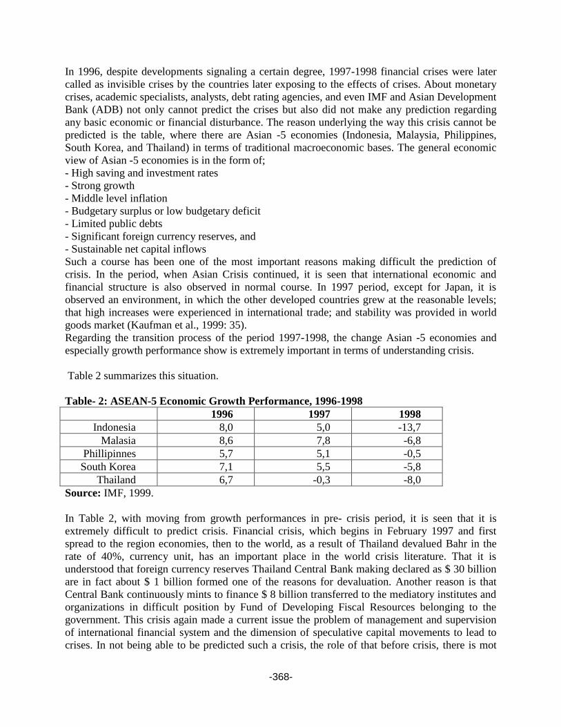
-368-

In 1996, despite developments signaling a certain degree, 1997-1998 financial crises were later

called as invisible crises by the countries later exposing to the effects of crises. About monetary

crises, academic specialists, analysts, debt rating agencies, and even IMF and Asian Development

Bank (ADB) not only cannot predict the crises but also did not make any prediction regarding

any basic economic or financial disturbance. The reason underlying the way this crisis cannot be

predicted is the table, where there are Asian -5 economies (Indonesia, Malaysia, Philippines,

South Korea, and Thailand) in terms of traditional macroeconomic bases. The general economic

view of Asian -5 economies is in the form of;

- High saving and investment rates

- Strong growth

- Middle level inflation

- Budgetary surplus or low budgetary deficit

- Limited public debts

- Significant foreign currency reserves, and

- Sustainable net capital inflows

Such a course has been one of the most important reasons making difficult the prediction of

crisis. In the period, when Asian Crisis continued, it is seen that international economic and

financial structure is also observed in normal course. In 1997 period, except for Japan, it is

observed an environment, in which the other developed countries grew at the reasonable levels;

that high increases were experienced in international trade; and stability was provided in world

goods market (Kaufman et al., 1999: 35).

Regarding the transition process of the period 1997-1998, the change Asian -5 economies and

especially growth performance show is extremely important in terms of understanding crisis.

Table 2 summarizes this situation.

Table- 2: ASEAN-5 Economic Growth Performance, 1996-1998

1996 1997 1998

Indonesia 8,0 5,0 -13,7

Malasia 8,6 7,8 -6,8

Phillipinnes 5,7 5,1 -0,5

South Korea 7,1 5,5 -5,8

Thailand 6,7 -0,3 -8,0

Source: IMF, 1999.

In Table 2, with moving from growth performances in pre- crisis period, it is seen that it is

extremely difficult to predict crisis. Financial crisis, which begins in February 1997 and first

spread to the region economies, then to the world, as a result of Thailand devalued Bahr in the

rate of 40%, currency unit, has an important place in the world crisis literature. That it is

understood that foreign currency reserves Thailand Central Bank making declared as $ 30 billion

are in fact about $ 1 billion formed one of the reasons for devaluation. Another reason is that

Central Bank continuously mints to finance $ 8 billion transferred to the mediatory institutes and

organizations in difficult position by Fund of Developing Fiscal Resources belonging to the

government. This crisis again made a current issue the problem of management and supervision

of international financial system and the dimension of speculative capital movements to lead to

crises. In not being able to be predicted such a crisis, the role of that before crisis, there is mot

-369-

any problem in the real economies of the countries suffering from crisis is large. In the countries

of the region, it is observed that foreign capital enterprise was encouraged before crisis. On the

other hand, it was observed that foreign capital going toward the countries such as South Korea,

Indonesia, Thailand, Malaysia, and Philippines had an important place in short term debt of the

relevant countries. The effect of Asian crisis on the real sector, especially on the stocks of the

firms, which are processed in stock markets, had been deep. After Asian crisis, in the stocks of

the companies being in active in the region, important falls occurred. In 1997, while one share of

Sampoerna, Indonesian Cigarette Company was about $ 6.75, it fell to 20 cent after crisis. While

the capital of the same company was $ 6 billion, 18 months later from the crisis, it regressed to $

200 million. On the other hand, while in the country, I Dollar = 2300 Rupee, then 1 $ = 14.000

Rupee had been. In general, as a result of crisis, in Hong Kong, Indonesia, South Korea, and

Thailand Stock markets, capital loss capital loss emerging in 1997 reached the level of $ 200

billion (Faber, 1998:73).

3.5. 2007-2008 Global Financial Crisis

In 2007, due to trouble experienced in sub-prime credits in financial institutes in US, a crisis

emerged, which first spread in US, then, all of European countries., and with contagion effect, all

over the world. Crisis in US emerged after disturbances in subprime mortgage markets. The

disturbance in these markets is a result of a process beginning 2000s. Technology balloon, which

reached quite high levels and exploded in 2001, can be seen as the first step in the process. That

is, with explosion of technology balloon, a number of technology company went bankrupt and

underwent important losses; thus, the companies such as Merrill Lynch were obliged to pay for

high indemnities. In order to remove the impacts of crisis and again raise decreasing demand,

Federal Reserve System (FED), discounting interest rate beginning from 2001, lowered interest

rates to the levels of 1%. After technology balloon exploded not only in America but also Europe,

central banks, being concerned about that deflation will occur, lowered interest rates from 2001

to 2005 (Goodhart, 2008: 332).

2007 Global Financial Crisis also brought together with it new changes in terms of risk models.

Bisias et al. (2012), in their studies, developed a broad model examination toward financial risk

indicators. This model is the one, which only focuses on financial risk measurements, is toward

measuring financial pressure, mostly contains sensitivity analyses, and refers to the systems such

as early warning system Mishkin (2009), with moving from the theoretical and empirical findings

regarding global crisis experienced, put in order 9 basic principles, which almost all central banks

agree with, as follows:

- Inflation is an omnipresent monetary phenomenon.

- Price stability has important benefits.

- In the long term, there is no trade off between unemployment and inflation.

- Expectations has an important role in the determination of inflation and transfer of monetary

policy to macroeconomic structure.

- According to Taylor rules, it is necessary to deal with interest rate together with high inflation.

- Monetary policy subjects to the problem with time inconsistency.

- Independence of central bank help the efficiency of monetary policy develop.

- In the core of the formation of results of good monetary policy, there is a strong commitment.

-370-

These principles, as stated in the studies of Goodfriend and King (1997), are the elements of

“new neoclassic synthesis” and they are the principles, which many central banks employees and

academics agree with before crisis (Mishkin, 2009: 68).

Global economic crisis led many economies in the world to enter a deep stagnation. The

disturbances occurring within EU with 27 members, 17 of which use Euro and 10, their own

money, together with global crisis, made survival of “Single Europe” ideal seriously questionable

.While the regression of share of active population in total reduces potential growth in these

countries, as a requirement of the principle “social state”, it also led expenditures on pension and

health system, whose control is difficult, to increase. While global economic crisis causes

economic growth to rapidly regress, with the effect of crisis, unemployment rate rapidly

increased.

4. EXPERIENCES OF FINANCIAL CRISIS FROM TURKEY

Turkish economy was exposed to the various crises in the various periods since announcement of

republic. It is observed that the crises experienced in the periods following Second World War

emerge in a surprising order. That is, Turkey experienced crises (1958, 1978, and 1998), which

can be deemed important, toward the ends of every decades. These ten year cyclical quality of

crises recalls an economic theory, which is -called “Juglar Waves” in the literature of cyclical

fluctuations, and which identify fluctuated growths of mature capitalist economies (Kazgan,

2005: 4).

In Turkey, the crises experienced especially 1990s, produced significant negativities on economy.

The major reasons of these crises experienced in Turkey is that an unsustainable domestic debt

dynamic and unhealthy structure in fiscal system, especially public banks, and the other structural

problems, cannot be united to a permanent solution. In addition to these, global qualified crises

created instabilities in Turkey, although there was no remarkable crisis in the dynamics of

economy. In Asian, Russian Crises, and financial crisis recently experienced, this case was

witnessed.

In the early 990s, stability programs applied in Turkey were carried out toward the solution of

problems we can put in order as reducing inflation, closing current account deficit, determination

of interest rates and exchanges rate realistically, and etc. However, it was concluded with

unsuccessfulness. The most important reason for this unsuccessfulness is that reforms cannot be

necessarily implemented and, more importantly, politic economy axis institutionalism cannot be

provided (Emsen, 2004: 87). These negative conditions obliged Turkey to apply two stability

programs, which are IMF-origin. In this scope, two standby agreements were signed with IMF,

the first of which was on the date of April 5, 1994 and the other, on the date of December 9,

1999.

4.1. 1994 Crisis

In 1994, Turkey, after an interval of 17 years, again faced with an economic crisis. That foreign

finance possibilities of economy are thoroughly constricted and that foreign debt services become

unsustainable, at the first look, show as if the crisis experienced in 1980 and 1994 Crisis are

similar to each other in terms of onset of crisis. However, in terms of either the reasons leading to

crisis and conditions reached in the peak point of the crisis or political and economic conjuncture,

-371-

where the world live, 1994 crisis is relatively different than 1980 crisis. 1994 crisis emerged

together with an intensive crisis. Differently from 1980s, in 1994 crisis, there is a case, in which

banking sector, non- banking private sector, and households are in debt and this debt is n terms of

foreign exchange. In 1994 Turkey, as in 1980s, bringing freedom on the subjects of the exchange

rate, interest, and prices, possibility to reform expired (Ekinci, 2001: 67).

Beginning from 1990, that public sector deficits rapidly rise caused public sector borrowing

requirement (PSBR) to increase and the rate of PSBR/GDP exceeded the level of 10%. As a

result of deficits resulted from current expenditures and transfer expenditures of public, the

increasing need for debt was tried to be financed by domestic and foreign borrowing. The

increase of total debt stock led the debt, capital, and interest payments to increase and especially

domestic debts and domestic interest rates to rise. In fact, tax incomes come on running short of

meeting even domestic debt service. In 1990, total domestic debts, whose share in GDP was

15.3%, reached the level of 17.9% in 1993 before crisis . In the same dates, the share of foreign

debts in GDP realized as 30.8% and 44.1%,. Financing foreign debt payments with domestic

borrowing left Turkey under a large domestic borrowing press in 1994, when crisis was

experienced. Thus, total domestic debts reached TL 656 trillion and the rate of domestic debts to

GDP rose to 18%, which is the highest level among developing countries. As a result of

excessive increases occurring in the debts of public sector, that the debt becomes unsustainable

showed itself with the crises experienced in December 1993 and April 1994. As a natural result

of increasing resource need, interest rates significantly rose as well and reached the level of

89.2% from its level of 58.9% in 1990. In the years of 1990, 1991, 1992, and 1993, when

considered that WPE (Wholesale Price Index) was 52.2%, 55.4%, 62.1% and 58.7%,

respectively, it is evident that real interest has considerably risen in the recent years (TCMB,

1993). While that real interest is too high leads to a positive effect in short term fund inflow, they

engendered crowding out effect on private sector investments. In order to prevent this state, the

efforts to lower interest rates with the pressure from private sector also beginning from the mid-

1993 formed one of the most important reasons for 1994 Crisis (Karluk, 2005: 411).

4.2. November 2000 and February 2001 Crisis

Turkey, on the dates of November 22, 2000 and February 21, 2001 met financial crises. It can be

said what underlying these financial crises is the troubles of liquidity and demand of foreign

currency. The difference of these crises from the previous crises is that these crises coincided

with the periods, when comprehensive stability programs were applied. The crisis occurring in

November 2000 is in a quality of continuation of 1994 Crisis and February 2001 is in quality of

the second wave of November 2000. After 1994 Crisis, overvaluation of TL continued, foreign

deficits increased and real interests rose. Together with Southeast Asian Crisis in 1997, and

Russian Crisis in 1998, concern of hot money from Turkey thoroughly increased (Ertuna, 2001:

494).

On November 23, 1999, a standby agreement, which will be valid, beginning from the early

2000, was signed; on the date of December 9, 1999, an intention letter was sent to IMF and

Central Bank declared monetary and fiscal policy of the year toward reducing inflation and

sustainable growth. Three year program, which has three main legs as providing fiscal discipline

in public sector, determining exchange rate with crawling peg previously determined, and

accelerating structural reforms and privatization, was implemented in the period of 2000-2002.

-372-

The main target of program is to lower inflation to a one –digit figure at the level of 5.5%, reduce

high real interest rate to a reasonable level, and provide the more effective and fair distribution of

resources in economy at the end of 3 years period (Yıldırım, 2001: 26).

5. COMPARATIVE ANALYSIS

Financial crises experienced incorporate the different dynamics in respect with the period, in

which they were experienced. Two basic model developed regarding the predictability of crisis

before emerging are the leading indicators and signal approach.

In order to be able to predict financial crises, setting out from the crisis experiences previously

experienced, the various indicators, which can posses have a quality of early warning, are used.

These indicators used in preventing crises point out which factors causes the most to crises.

The factors increasing vulnerability in an economy can be put in order in the form of (IMF,

1998);

-Inconsistent macroeconomic policies

-Wrong applications of exchange rate,

-Foreign financial conditions (terms of trade, world interest rates)

-Structure and terms of capital movements

-Shifts in market expectations

-Weakness of financial sector, and

-Political factors

According to KLR model, known as signal model, each variable is analyzed and suitable

threshold values are calculated. That any indicators go up threshold value or goes down threshold

value is accepted as crisis signal. For overcoming the problem with determining threshold

correctly, independent variable series is divided into percentage shifts. According to the direction

of independent variable to affect dependent variable, the most suitable slice is determined as

lower and upper threshold. For example, if slice of 10% will be used ,when lower threshold is

determined, the case of falling below the slice of 10% is perceived as crisis signal, while upper

threshold is determined, the case of going up the slice of 10% is perceived as crisis signal and the

probability to experience crisis in the future 4 months can be predicted.

In KLR Model, with the deviation of PPD index by 3 Standard Deviation from the mean deviates,

signal months obtained from the leading indicators are compared on Social Crisis matrix in Table

3.

Table- 1: Signal Crises Matris

Signal There is a crises (in

24 month)

Theris no crises (in 24

month)

YES A B

NO C D

Source: Kaminsky and Reinhart, 1999.

-373-

In application, there are a number of studies using KLR models. Berg and Pattillo (1999)

compared regression models with KLR Model and searched for an answer to question whether or

not Asian Crisis can be predicted. The study results showed that KLR model was more successful

in the prediction of Asian Crisis compared to the other ones. However, since the wrong signals in

the model is more than the right signals, in determining the time of crisis in 1997, it was also

stated that KLR Model is not reliable enough. However, in both models, in cases, in which high

current deficit is n important risk factor; domestic credits are high; and the real exchange rare was

overvalued; and M2 / Reserves Ratio increases, they stated that the possibility of monetary crisis

to appear could show an increase.

Edison (2000) defined the crisis in the form of that national money undergoes to a sharp

devaluation and that international reserves decreases and used KLR Model. Edison, differently

from the other studies, increased the number of country and considered the regional differences.

He utilized in the study the variables such as deviation in exchange rate, export and import

values, foreign currency reserves, M2/Reserves, difference of the domestic and foreign deposit

interest rates, industrial production index, bond prices index, M2 multiplier, domestic

credits/GDP, real deposit interest rate, credit interest rate/deposit interest rate, M1 balance, and

commercial bank deposits. Edison (2000), in order to be able to identify crisis months, taking

weighted mean of the percentage variation in exchange rate and parentage in foreign reserves,

formed a foreign currency market pressure index. Devaluation of national money and fall of

reserves raise foreign currency market pressure index. That foreign currency market pressure

index goes up the mean by 2.5 standard deviation (SD) was defined as crisis. The threshold value

accepted as 2.5 SD was intuitively determined. As a conclusion of the study, it was observed that

KLR model, also in cases, in which there is no crisis, may give the wrong signals. According to

Edison, this case shows the weakness of model. KLR Model, as an approach of leading

indicators, may be an alternative to probit models used by IMF. Edison emphasizes that this

method having an advantage due to the fact that more variables are available, in case that

variations in exchange rate as well as variations in interest rates and inflation rate is included in

it, can give better results.

Goldstein et al. (2000) , for the period of 1970‐1995, further enlarging the monthly basis

indicators of 25 countries used by Kaminsky and Reinhart (1999) in predicting financial crises

for the period of 1970-1995, made a prediction via signal approach. They suggested that in

banking crises, the variables of real exchange rate, stock prices, monetary multiplier, production

increase, and export indicators gave crisis signal, while in monetary crises, real exchange rate,

stock prices, export, M2/reserves, and production increase are the indicators signaling crisis

(Goldstein et al., 2000: 56).

Peng and Bajona (2008) attempted to predict the monetary crisis experienced by means of KLR

Model, using the data of the period June 1991- November 2001 of Chinese economy. KLR

Model became successful in predicting 1994 exchange rate fluctuations and August 1998 and

May 1999 Asian Crises. However, China, due to capital supervisions it has applied and lack of

convertibility, in Asian crises, did not experience a full monetary crisis. As a conclusion of the

study, some suggestions are made related to the future policies of China regarding Asian crisis.

First is that the weak structure of China in financial system and vulnerable structure of banks

continue. Therefore, there is a need for rearranging banking system. Secondly, the awkward

structure of government enterprises is criticized and emphasized that it is necessary to produce

-374-

policy toward this. Lastly, it is argued that foreign exchange regime of China is its distinctive

feature from the other countries. Therefore, in case that China gives up its exchange rate policies,

it is noted that it will have more vulnerable structure against crises.

Shi and Gao (2010), in their studies, in 2008 Crisis, utilizing the data regarding 13 countries

(Chili, Euro, Zone, India, Island, Japan, Korea, Malaysia, Mexico, Pakistan, Russia, Vietnam,

United Kingdom, and US), tested KLR Model. Export, credit interest rate, deposit interest rate,

M2/reserves, production index, and bond prices index were found as indicators, whose success is

the highest in preventing the crises. What underlying of that many researchers using KLR model

use Dollar as currency is the assumption that American economy and the value of Dollar is

stable. However, in some studies, with the use of SDR instead of $, analyses were repeated and it

was put forward that the results founded were more successful than in the prediction of crisis.

In this study, among the crises included in the sample, ERM crisis is originally currency / foreign

currency crisis. In Mexican economy, in 1970s, while the process beginning together with the rise

experienced in oil prices, on the one hand, increases oil incomes of the country, on the other

hand, it led to a serious disturbance in the fiscal discipline. As a result of this, in December 1994,

Mexico, obliging to devalue its national currency unit, faced a financial crisis and this crisis

resulted in a big economic collapse.

1998 Asian Crisis continued together with a banking crisis accompanying to monetary crisis. In

this scope, this led a sort of crisis qualified as twin crisis to be included in the literature. In 2007,

in the financial organizations, due to malfunction experienced in sub-prime credits, a crisis

occurred, which especially spread to US, then, European countries, and with the contagion effect,

all over the world. It is observed that the crises experienced in Turkey basically arise from not

being able to apply the adequate reforms regarding financial system and weakness of the

resistance against financial vulnerabilities.

CONCLUSION AND DISCUSSION

In post 1990 period, although the crisis experienced is seen to be resulted from the different

dynamics, it is also to mention about some common features they basically show. Since the

crises, collected under the title of “Three Generations” form as a result of its showing differences

from the crisis concept before it in respect with the periods, it is possible for it to include the

feature resembling to the previous generation. Approach of logit and probit models toward

predicting crisis probability of empirical literature regarding crises, largely suggested by Franlel

and Rose, was shaped on the axis of the studies on the roots and spread of the crisis in the

leadership of Sachs et al. (1996) and statistical studies carried out by Kaminsky et al. (l998) and

known “signal approach”

As a result of overvaluation of currency, depending on the demand of import, they examined the

problem with being able to rotate the emerging debts in case of referring to foreign borrowing for

financing import and the process continuing in the form of the problems that foreign trade deficits

reach the extreme dimensions arise on the axis of first generation monetary crisis models. The

process, in which speculative foreign currency attacks begin, central bank avoid interventions

toward protecting reserves, and crisis is directed according to the expectations of economic actors

was called as second generation monetary crisis and this model was used in explaining monetary

-375-

crises (e.g. 1992-1993 ERM crises) occurring in the developed countries. Finally, the models,

which accept onset of crisis as expectation, put forward that this is followed by the problems

experienced in banking sector and the problems resulted from international financial system, and

which is developed to be able to account for 1998 Asian Crisis were called as third generation

monetary crises.

REFERENCES

1. Berg, Andrew and Pattillo, Catherine (1999), “Are Currency Crises Predictable? A Test”,

IMF Staff Papers 46(2), 107-138.

2. Bordo, Michael D. (1986), “Explorations in Monetary History: A survey of The Literature”,

NBER Working Paper, 1821, 1-104.

3. Cobham, David (1996), “Causes and Effects of the European Monetary Crises of 1992-93”,

Journal of Common Market Studies, Wiley Blackwell,34(4),585-604.

4. Davis, E.P. (1992), Debt, Financial Fragility, and Systemic Risk, Oxford, Clarendon Press.

5. Dornbusch, Rudiger, Werner, Alejandro, Calvo, Guillermo and Fischer, Stanley (1994),

“Mexico: Stabilization, Reform, and no Growth”, Brookings Papers on Economic Activity,

(1), 253-315.

6. Dorukkaya, Şakir and Yılmaz, H. Hakan (1999), “Liberalizasyon Politikaları Aşırı Borçlanma

Sendromu ve Arkasından Yaşanan Finansal Krizler (Şili ve Meksika Deneyimleri)”, Yaklaşım

Dergisi, 7(75), 122-127.

7. Edwards, Sebastian (2001), “Exchange Rate Regimes, Capital Flows and Crisis Prevention”,

NBER Working Paper, 8529, 1-69.

8. Ekinci, N. (2001), “1992’den 2001’e Ekonomik Kriz”, Görüş Dergisi. 15.

9. Ertuna, Ö. (2001), “Türkiye’de Ekonomik Krizler, Nedenleri ve Çıkış Yolu”, Yeni Türkiye

Dergisi, Ekonomik Kriz Özel Sayısı, 44, 491-510.

10. Faber, Marc (1998), “Ben Graham in Asia”, Forbes Global Business and Finance, 10, 73-74.

11. Friedman, Milton and Schwartz, Anna J. (1963), A Monetary History of the United States:

1867-1960. Princeton: Princeton University Press for NBER.

12. Goodfriend, Marvin and King, Robert G. (1997), The new neclassical synthesis and the role

of monetary policy. http://www.nber.org/chapters/c11040, 231-296.

13. Goodhart, Charles and Bin Lim, Wen (2008), “Do Errors in Forecasting Inflation Lead to

Errors in Forecasting Interest Rates?”, Discussion paper, 611, Financial Markets Group,

London School of Economics and Political Science, London, UK.

14. Goldstein, Morris and Turner, Philip (2004), Controlling Currency Mismatches in Emerging

Markets, Institute for International Economics, Washington.

15. Gurvich, Evsey, Pinto, Brian and Ulatov, Sergei (2004), Lessons from the Russian Crisis of

1998 and Recovery, The World Bank Publications.

16. IMF, (1998), World Economic Outlook, Financial Crises: Causes and Indicators.

17. IMF, (1998), World Economic Outlook, Origins of Currency and Banking Crises.

18. IMF, (1999), World Economic Outlook, Financial Turbulence and the World Economy.

19. Karluk, Rıdvan (2005), Cumhuriyetin İlanından Günümüze Türkiye Ekonomisinde Yapısal

Dönüşüm, Beta Yayınevi, İstanbul.

20. Kaminsky, G. and Reinhart, Carmen M. (1999), “The Twin Crises: The Causes of Banking

and Balance Of Payments Problems”, The American Economic Review, 89(3), 473-500.

21. Kaufman, G.G., Krueger, T.H. and Hunter, W.C. (1999), The Asian Financial Crisis:

Origins, Implications and Solutions, Springer.

http://ideas.repec.org/a/bla/jcmkts/v34y1996i4p585-604.html

http://ideas.repec.org/s/bla/jcmkts.html

http://www.nber.org/chapters/c11040

http://eprints.lse.ac.uk/24432/

http://eprints.lse.ac.uk/24432/

-376-

22. Kindleberger, Charles P. (1978), Economic and Financial Crises and Transformations in

Sixteenth-Century Europe, International Finance Section, Department of Economics,

Princeton University

23. Minsky, Hyman P. (1972), Financial Instability Revisited: The Economics of Disaster,

Fundamental Reappraisal of the Discount Mechanism, Board of Governors of the Federal

Reserve System, Washington.

24. Mishkin, Frederic S. (1996), “Understanding Financial Crisis: A Developing Country

Perspective”, NBER Working Paper, 5600, 1-55.

25. Moussalli, Cinzia B. (2008), “Solving the Current Account Puzzle: Capital Flows and the

Contagion Effect of Financial Crisis”, Journal of Economics, Banking and Finance, 2(1), 1-

14.

26. Peng, Duan and Bajona, Claustre (2008), “China's Vulnerability to Currency Crisis: A KLR

Signals Approach”, China Economic Review, 19(2), 138-151.

27. Pilbeam, Keith (1998), International Finance, Second Edition, Macmillan Press Ltd.,

London.

28. Schwartz, Anna J. (1986), Real and Pseudo Financial Crisis, (Ed.: F. Capie and G. E. Wood).

Financial Crises and the World Banking System, Macmillan, London, 11-31.

29. Shi, J. and Gao, Y. (2010), “A study on KLR Financial Crisis Early-Warning Model”,

Frontiers of Economics in China, 5(2), 254 – 275.

30. Szczurek, Mateusz (2003), International Liquidity and Currency Crisis Costs: Currency

Crises in Emerging Markets, (Ed.: Marek Dabrowski), Kluwe Academic Publishers,

Dordrecht.

31. TCMB, (1993), Aylık İstatistik Bülteni, Aralık, Ankara.

32. Yıldırım, M. (2001), “Para kurulu ve Kasım 2000 Krizi”, Gaziantep Üniversitesi Sosyal

Bilimler Dergisi, 4(2), 17-37.

http://www.sciencedirect.com/science/article/pii/S1043951X07000491

http://www.sciencedirect.com/science/article/pii/S1043951X07000491

http://www.sciencedirect.com/science/journal/1043951X

-377-

COMPARISON OF THE SOCIO-ECONOMIC DEVELOPMENT AND THE PISA

RESULTS OF OECD COUNTRIES

Hasan Bulut



Yüksel Öner


Abstract

The PISA test has been conducted over a period of three years since 2000 in many countries, both

OECD countries and non-OECD countries. In this test, students in the 15-year-old group are

asked questions about their "Reading Skills", "Mathematics literacy" and "Science Literacy" in

their native language. Undoubtedly, the future of the countries is closely related to the success of

the younger generations in the basic fields. Countries are planning to develop socio-

economically. This study aims to compare the PISA scores and socio-economic development of

OECD member countries.

Key words: OECD, PISA, Socio-Economic Development.

1. INTRODUCTION

Undoubtedly, the development of the countries and the increase in the level of welfare depend on

the quality of the education given to the youth. The presence of quality education will bring

society forward not only economically but also socially and culturally. The Organization for

Economic Cooperation and Development (OECD), which is also a member of Turkey, has been

conducting various tests with the Program of International Student Assessment (PISA) since

2000, for students aged 15 years in countries with and without memberships [1].

The aim of this study is to calculate the results of the PISA test in 2006, 2009 and 2012 for the

OECD member countries by using the Data Envelopment Analysis method, which is the input of

the Dependent Population Ratio, Gross National Income and High Technology Exports variables.

The PISA test is conducted so that each country can see the deficiencies in the education system

and make the necessary adjustments, not for the countries to compete with each other. The

questions asked in the PISA tests are not based on the curriculum shown in the school but on the

responses to situations and problems that a student trained in his / her country until the age of 15

may face in daily life. In other words, a 15-year-old educated young person demonstrates how

much he prepared for the rest of his life, even if he did not continue his education. The PISA test

measures mathematics literacy, science literacy and reading comprehension.

-378-

2. DATA ENVELOPMENT ANALYSIS

Data envelopment analysis is a method developed to measure the relative effectiveness of

decision-making units (DMU) [2]. The goal is to demonstrate how successful it is in converting

the available inputs (resources) into the outputs of the DMUs. The input and output of DMUs

must be the same and measured in all cases. Another advantage of DEA is that very different

measurement units for input and output variables can be used at the same time [3].

The efficiency score for the DMU is calculated as in Equation (1) when there are m inputs

and outputs.

where

: The amount of output produced by the DMU for 𝑟=1,…,𝑠

: The amount of input used by the DMU for 𝑖=1,…,𝑚

: The weight coefficient given by the DMU to the outputs for 𝑟=1,…,𝑠

: The weight coefficient given by the DMU to the inputs for 𝑖=1,…,𝑚

The constraints for Equation (1) are denoted as [2]:

and

In DEA, if a DMU's efficiency score is 1, it is efficient, otherwise it is not. There are generally

three methods used in the DEA:

i. CCR (Charnes-Cooper-Rhodes) Method (1978)

ii. BCC (Banker-Charnes-Cooper) Method (1984)

iii. Additive Method

The first two methods have been used in this study. In the CCR method, there is a fixed yield

according to scale assumption, while in the BCC method there is a changing-based yield

assumption. Also, the BCC limit is always below the CCR limit. For this reason, the CCR

efficiency score is less than or equal to the BCC efficiency score [4].

Moreover the results can be interpreted in two different ways in CCR and BCC models: input-

oriented or output-oriented. In the input-oriented approach, it is aimed to minimize inputs to meet

the same output level. In the output-oriented approach, the aim is to maximize the output value

with the available inputs [5].

3. APPLICATION

The data used in the study are compiled from two different sources. The data sets for the

Dependent Population, Gross National Income and High Technology Exports variables used as

input variables in the study are obtained from the World Bank website [6]. The output variables,

PISA Mathematics, Science and Reading comprehension variables are taken from the OECD [7].

-379-

Only OECD countries have been included in the study. 2006, 2009 and 2012 were taken as the

working period. Because USA did not participate in the reading-comprehension part of the PISA

test in 2006, there is not USA in results of 2006. Furthermore, in DEA, output-oriented CCR and

BCC models are used. The results are given in Table 1.

When Table 1 is investigated, it is showed that Hungary, Korea Republic and Slovak Republic

are efficient countries according to all periods and methods. While Estonia is not only efficient

according to CCR method in 2012, it is efficient in all other periods and methods. According to

the BCC method, Finland and Netherlands are efficient in all the years. Slovenia is efficient in

2006 and 2009, not 2012. On the contrary, Sweden is not efficient in 2006 and 2009 and is

efficient in 2012. Similar comments can be made for other countries. Contrary to what is

expected here, socio-economically developed countries such as USA, UK, France, Germany and

Italy have never been efficient. Turkey is also one of countries that have never been efficient at

any time.

Table 1: DEA Results

COUNTR

IES

2006 2009 2012

CCR BCC CCR BCC CCR BCC

Australia 0.893727 0.994235 0.868854 0.993308 0.841949 0.989521

Austria 0.854166 0.938732 0.796893 0.924969 0.812328 0.957448

Belgium 0.784106 0.948921 0.767526 0.949616 0.753619 0.969206

Canada 0.955896 0.99864 0.930846 1 0.900525 0.99973

Chile 0.91296 1 0.922601 1 0.882897 0.89848

Czech

Republic 1 1 0.931903 0.979397 0.835557 0.958778

Denmark 0.796748 0.947557 0.748049 0.929394 0.739238 0.955625

Estonia 1 1 1 1 0.864367 1

Finland 0.901036 1 0.858362 1 0.76644 1

France 0.69407 0.903676 0.674325 0.921078 0.639545 0.940045

Germany 0.758367 0.918726 0.714448 0.945913 0.697854 0.964675

Greece 0.784565 0.889849 0.874793 0.923999 0.761149 0.925547

Iceland 0.88891 0.940154 0.865621 0.976244 0.78518 0.943764

Hungary 1 1 1 1 1 1

Italy 0.952598 0.995248 0.850858 0.96136 0.762926 0.994547

Israel 0.607551 0.836183 0.627704 0.893911 0.630638 0.925463

Ireland 0.742367 0.854594 0.729978 0.90564 0.759673 0.938596

Japan 0.757669 0.953943 0.709844 0.976632 0.691039 1

Korea,

Rep. 1 1 1 1 1 1

Luxembou

rg 0.885508 0.951634 0.943433 0.957132 1 1

Mexico 0.55157 0.747178 0.582932 0.791653 0.637769 0.800948

New

Zealand 0.831077 0.967994 0.80438 0.967702 0.742487 0.971511

Netherland 1 1 0.986629 1 0.898325 1

-380-

s

Norway 0.78518 0.928798 0.787179 0.950898 0.804064 0.969895

Poland 0.87033 0.972928 0.89404 0.955683 0.990112 1

Portugal 0.961507 0.966621 0.977911 1 0.764189 0.942074

Slovenia 1 1 1 1

0.802

04

0.926

431

Slovak

Republic 1 1 1 1 1 1

Spain 0.859094 0.913138 0.82828 0.923289 0.797452 0.934086

Sweden 0.782681 0.926814 0.746656 0.926874 1 1

Switzerlan

d 0.868464 0.96996 0.848158 0.983623 0.869917 1

Turkey 0.71111 0.855994 0.810777 0.886986 0.78789 0.928781

United

Kingdom 0.741898 0.913816 0.755942 0.927798 0.711267 0.944498

United

States * * 0.731934 0.928502 0.699946 0.92669

4. CONCLUSION

As mentioned earlier, the PISA test is not done for countries to compete with each other. The aim

of the test is to determine the deficiencies in the education systems of the countries and to go

about them. When Turkey's 2006, 2009 and 2012 PISA results are examined, it is seen that there

has been an improvement in recent years. However, success in terms of effectiveness still does

not seem close. For this reason, the education systems in the countries which are efficient should

be examined and necessary arrangements should be made. Scandinavian countries, such as the

Czech Republic, Estonia, Finland, Slovenia, Sweden and Switzerland, seem to be active,

according to different periods and methods. For this reason, we should first examine the

education system in Scandinavian countries and make the necessary arrangements in our country

and show our young people that we hope to develop our country the better chance of preparing

for the future.

REFERENCES

1. http://pisa.meb.gov.tr/?page_id=22 (Accessed: 09.10.2016)

2. Şenel T. and Gümüştekin S. (2015) "Evaluation Of The Efficiency Of Hospitals In

Samsun Using Data Envelopment Analysis." International Anatolia Academic Online

Journal, Volume:3-2, page:53-60.

3. Özden, Ü. H. (2008) “Efficiency evaluation of foundation universities in Turkey by using

Data Envelopment Analysis (DEA)”. İstanbul University Journal of Faculty of Business,

37(2), 167-185.

4. Dinçer, E. S. (2008) “Examination of Total Factor Productivity change by Mamwuist

Andex in Data Envelopment Analysis and an Application on İstanbul Stock Exchange”.

Marmara University Journal of Faculty of Economics and Administrative Sciences, 25(2).

http://pisa.meb.gov.tr/?page_id=22

-381-

5. Okursoy, A. and Tezsürücü, D. (2014) “Comparison of the Relative Efficiencies by the

Data Envelopment Analysis: An Application in Turkey for the Provinces of Cultural

Indicators” Journal of Management & Economics, 21(2).

6. http://www.worldbank.org/ (Accessed: 09.10.2016)

7. https://www.oecd.org/ (Accessed: 15.10.2016)

http://www.worldbank.org/

https://www.oecd.org/

-382-

OBSTACLES IMMIGRANTS FACED IN INTEGRATION TO LABOR MARKET: THE

SAMPLE OF SYRIAN IMMIGRANTS IN TURKEY

Sefa Çetin

Kastamonu University, Turkey


Hasan Hüseyin Büyükbayraktar



Abdullah Yilmaz



ABSTRACT

The integration of immigrants into the labor market in economic sense makes it possible for the

immigrants to maintain their lives by earning their income.This labor market integration is

extremely important for the fact that this integration paves the way for both immigrants and the

native people to live together in peace and prosperily. With this in the mind, the aim of this study

is to establish the obstacles which are encountered by the immigrants in the process of integration

into host country labor market. For this purpose, primarly, these obstacles investigated by

lliterature review. Then, the obstacles which are faced by Syrian immigrants living in Konya

province have been determined by a qualitative study. The sample of this study consists of the

Syrian immigrants (n=20) living in Konya province. For this study, Qualitative data was

collected through semi-structured interview forms. As the conclusion, the most important

obstacles appeared are as follows; wages lower than they deserve, remaining in the event of non-

payment, abuse by employer in terms of excessive working hours and heavy working conditions,

lack of work safety and continuity, abasement in the workplace envoriment, difficulties related to

not knowing the Turkish language and not having the opportunity of practicing their profession,

so having feeling of propertylessness. These obtacles are largely similar with the ones

experienced by immigrants in other countries.

Keywords: Immigrant, Syrian Immigrants, Labor Market, Integration, Obstacles.

1. INTRODUCTION

Problems caused by the movement of immigrants, especially in the recent period, have not stood

out so much on the agenda of world countries, both Turkey and Continental European countries.

At the beginning of these problems, come socio-economic problems the countries that accept

immigrants in large numbers face with. At the beginning of these problems, come socio-

economic problems the countries that accept immigrants in large numbers face with.

-383-

In this context, it is clearly an essential requirement that the problems that may be caused because

of participation of immigrants into the labor market must be minimized, ensuring effective and

efficient participation of immigrants into the labor market and managing this process, in the long

term, in order to ensure a positive contribution to the national economy.

2. THEORETICAL FRAMEWORK

2.1. Labor Concept

The population of a country is divided into two as the working age population (15-64 ages) and

non-working age population. Those who are in the working age group, who desire to work and

have the power are called as labour force. In a country, whole labor force is required to be

working. Namely, it is desired to have full emploment, to have zero unemployment. We gain the

amount of unemployed when we remove those who are employed from the labor force (Yavuz,

2012). "Labor force" is people at an age of either who are working at a productive work, or who

are looking for a productive job, who can work. Unless otherwise stated, it is the age of 15 and

over. The difficulty of finding a productive job is a phenomenon at the world level. Global forces

-commerce, capital and cross-border movement of labor- have important effects on employment

in the national economy (Çolak, 2010). Employment, economically, can be defined as operating

of production factors or to make them operate in order to gain profit. It is discussed in this

concept whether the production factors are used in the production of goods and services.

However, while only a loss in economic sense is in question when the labor force remains idle

through not being used in producing of production factors other than labor, labor force's staying

out of production, in other words, unemployment accompanies socio-political issues too(Germir,

2012).

2.2. World Countries’ Labor Force Structure

Countries throughout the world are divided into seven classes as developed, Central and Eastern

Europe, former Soviet Union countries, other high-income countries, oil-exporting developing

countries, middle-income developing countries, less developed countries. Turkey is among the

middle-income developing countries. The most striking image related to the world labor force is

the congestion poor countries. While 75% of rate in the labor force participation is in developing

countries (Middle-income developing countries and less developed), less than 15% is in

developed countries. China and India are home to 40% of the world's workers(Çolak, 2010).

2.3. Turkey’s Labor Force Structure

Although a significant portion of employment in the agricultural sector in Turkey, the low level

of labor productivity and the inability to create new job areas is also among the structural features

of employment (Germir, 2012).

In the scope of labor statistics in September 2015 period made by Turkey Statistical Institute

(TSI), across Turkey; while unemployment rate among age 15 and over was %10.3, among 15-24

age group it was 18.5%, and in 15-64 age group it was 10.5%, in the same period, the rate of

unregistered workers was 34.8% (TUIK, 2015).

-384-

2.4. Labor Force Structure of Konya

As of 2013, in Konya and Karaman region constituting 3.2% of the population of Turkey, the

employment rate with 46.4% is above the average of Turkey which is 45.9%. The unemployment

rate is 4.7%, and is is lower than other regions. While it was observed that the services sector

with 42.6% of the sector has the highest share in employment in Konya-Karaman region, he share

of the agricultural sector 32.7%, and the share of the industrial sector is 24.7%. Between 2004

and 2013, when examining the change in the sectoral composition of employment over the years,

it is observed that there has been an increase in the share of services and industrial sectors, and a

significant decline is observed in agricultural sector (TUIK, 2014).

It is observed that, when analyzed by sector distribution, under the Labour Market Research

Report involving a total of 3995 work in the private sector issued by Konya Provincial

Directorate of Labour and Employment Agency between 16 March-30 April, the most places of

business in manufacturing sector (1342), respectively, wholesale and retail trade (970),

construction (637), transportation and warehousing (213).

The least business sectors are cultural, atr, entertainment and sports (11), water supply, sewage,

waste management (8), electricity, gas, steam and air conditioning production and distribution(8).

In businesses under the research, a total of 127 thousand 310 people work, 85.2% of employees

were males, 14.8% are women (proportion of women in Turkey is 27.5'tir%). Within the

research, the businesses were asked vacant jobs, 2828 vacancies were identified, and 57.9% of

them in manufacturing, 20.4% in wholesale and retail trade, 7.2% is in construction sector (İşkur,

2015).

2.5. Obstacles The immigrants Face In Labour Market Integration

The labor market integration of immigrants has a great importance. Because their integration to

the labor market will provide them with sheltering which they need, safety and self-sufficiency in

the sense that they can maintain their lives (Brenke, 2015). Immigrants' integration to the labor

market is extremely important for the reason that it provides a basis for them to live in peace and

quiet with the natives of the countries they emigrate to and their social adaptation on cultural

facts.

It should not be ignored that short-term expenditures made for the immigrants for housing and

labor market integration are the investments for the future. In the long term, it will have a positive

contribution of immigrants to the economy of the country they emigrate to (Fratzsch and Junker,

2015).

To be included in the society in which they emigrate represents a multidimensional and a very

complex process. Immigrants can be involved in the community in which they emigrate in the

context of social, cultural, political and economy. Migrants often face with unemployment in the

labor market, they are obliged to accept low-paid and unskilled jobs (Ulukan, 2008).

Some researchers draw attention to that immigrants tend to concentrate in different business

sectors compared to domestic workers in the USA. Immigrants tend to fill short-term

manufacturing and daily work positions especially relatively low-paid and do not require higher

-385-

skills, but it seems that the longer the duration of their stay in the US, their participation in

similar sectors and jobs with local workers is possible in the labor market (Abowd ve Freeman,

1991: 306.).

Immigrants' individual characteristics determine their occupational mobility and earnings. Human

capital owned by immigrants (education, skills, work experience and knowing the language of the

society in which they emigrate) affect the economic success in society they emigrate(Chiswick,

1978).

The smaller the cultural and linguistic differences among the natives with immigrants, in other

words, the immigrants as they embrace the indigenous culture, and learn the language,

differences in economic opportunities will disappear over time (cited in Portes and Zhou, 1992).

The effective factors in the participation of immigrants in the labor market are age and gender.

According to available data, more than half of the immigrant job applicants are under the age of

34. However, the main factor is not to have necessary skills for the job such as to know the

language. Over time, these obstacles faced by immigrants will tend to decrease, and employment

opportunities will increase (Fratzsch and Junker, 2015).

An experimental study has revealed that an immigrant can have equal income to the domestic

labor at the end of 15 years (Chiswick, 1978).

Educated immigrants are the preferred source of labor for employers. Immigrants are working in

jobs below their skills in low quality jobs in the first. This case is observed particularly in periods

when mass migration is experienced and intensive labor supply is needed. Unregistered and low-

paid work is seen as a survival strategy. Intensely, they can get jobs in manufacturing, service and

construction sectors (Ulukan, 2008).

According to Kömürcü's study (2011), immigrants should accept, adopt the city and the country

in which they will live, and they should be aware that they are members of the place they live in.

Immigrants are solving their job problems through informal sector mainly. One of the best known

works of the informal sector, construction labor stands out. Construction labor is a labor-intensive

job. Namely, it is based on arm strength. It does not require education or a specific expertise.

Thus, the construction labor is an important area of employment for immigrants. Although the

sector provides unskilled, uneducated people and people who have no expertise in any area with a

job, in time, specialisation may occur in some businesses within this sector. The research has

denoted that more than half of the immigrants, when they first arrived, they started their working

life as a construction worker, but over time, there has been work specialization among them in

the construction industry (Uslu, 2012).

The vast majority of Syrian refugees in Lebanon find jobs in construction and agriculture sectors.

They can mostly receive seasonal, short-term and the average monthly wage of 290 dollars

without any formal employment contract. The said fee is approximately 40% lower than

minimum wage of a Lebanese employee. As a result of the increase in the supply of unskilled

labor, working daily wages of unskilled workers in Lebanon have decreased by 60% compared to

the previous situation prior to the start of the Syrian crisis. Syrian immigrants have become more

willing to work under lower wages, longer working hours. This case has led Lebanese, who didn't

-386-

want to give rein to Syrian refugees to get their jobs, to accept to work for lower wages and

difficult working conditions (Cited in Lewis, 2015).

When the business relationship feature between employers and immigrant workers is analyzed,

this relationship seems to be far away from the legal basis. The lack of legal basis of this

relationship makes the immigrant workers bonded to the employee, immigrants are given jobs

rather than domestic workers so that labor costs are reduced. Immigrant workers are made work

very long hours during the day by force when necessary. For there is a large number of illegal

immigrant workers wandering around unemployed, these put pressure on those who received the

work, immigrant workers who are given a job are made for 1-2 months and are fired, and the post

is filled with new ones immediately. These workers, who do heavy work very long hours during

the day, are mostly paid less than the commitment wage, sometime they aren't paid at

all(Akpınar, 2009).

A study made by Ekiz-Gökmen (2011) revealed that the immigrant women living in Marmaris

generally work in guiding, tour operating, animation due to the touristic structure of the region,

so that they provide cheap labor supply in the tourism sector, they are not paid properly while

working in jobs that do not require a qualification, or they cannot get their wages on time, they

were subjected to verbal and physical abuse, and they work unsecured under unhealthy

conditions. Working in unskilled jobs in question far from the training they received leads

immigrant women to become unqualified. The most important problem educated immigrant

women face in the labor market is to become unqualified through being given work in low-skilled

jobs with low wages.

According to the research Dedeoglu made (2011) in the province of Istanbul, Azerbaijani

immigrants sustain their lives working in garment factories, and under favour of this labor

supply, they are contributing to one of Turkey's most important sectors to become a global export

champion. But this contribution results in that Azerbaijani immigrant women and children remain

outside the social life, being an Azerbaijanese means working in apparel sector for half price,

sometimes nonpayment of wages, and sometimes exposure to physical and verbal violence. The

experience of migration experienced by the Azerbaijani families in Istanbul and social exclusion

affect negatively not only adult immigrants but also the new growing generation. Exclusion from

education and health services increase the risk of being faced with poverty and social exclusion

of more needy children to these facilities again in the future.

In the labor market of Germany, the research on women workers in the cleaning sector, who

emigrated from Turkey, shows that Turkish immigrant women have concentrated in cleaning

sector, the immigrant women got jammed in the said sector, discrimination based on ethnicity

and gender in the labor market occupied an important place, the cleaning sector is expanding and

while profit rates are increasing, the same percentage isn't increasing in employment, the reason

for this is the increasing levels of exploitation in in this sector based on low-wage immigrant

labor force, and the work is getting intense day by day (Ünlütürk- Ulutaş, 2013).

2.6. Barriers Syrians Immigrants Face within Their Integration to Turkey Labor

Market

"Arab Spring" term was first etched in our mind with the emerging of revolt movement against

the government in Tunisia on 18/12/2010, then it became a term we encountered as a result of the

-387-

popular uprisings it caused in countries such as Egypt, Libya, Syria in the first place, Jordan,

Algeria, Yemen and Lebanon, and unfortunately, after its negative effects for our country

especially after the influx of refugees caused by the crisis and the developments in Syria.

Within the time from 15 March 2011 till today, as of 29 January 2016, about 2 million 582

thousand in Turkey, and 50.224 Syrian refugees are residing in the province of

Konya(www.goc.gov.tr), and unfortunately, every day they lose a little bit of hope to return to

their homeland.

The most important problems faced by Syrian refugees under protection in Turkey we come

across are as registration, child protection, education, protection of women, health and labor

market access issues. In terms of participation in the labor market, registered Syrians can apply to

Labour and Social Security Ministry for a work permit in the sectors, business lines and

geographical areas (like cities, districts, villages) the Council of Ministers will determine. In this

regard, the legislation related to businesses and professions foreigners cannot work is reserved

(Karaca ve Doğan, 2014).

Within the scope of Karaca ve Doğan's study (2014), the obstacles Syrian refugees faced in their

integration into the labor market can be listed as follows:

-Difficulty in using the banking system of businessmen from Syria, other banks do not open

accounts for Syrian refugees except a few banks,

- Strict regulations in front of performing their professions who have competence and ability to

perform their specialty professions (pharmacy, dentistry, etc.), an immigrant who was educated at

a university and received a diploma in pharmacy cannot perform his/her profession, or cannot

work in a job related to the field, not to be allowed this by the legilation,

- Non-permanent (seasonal) working conditions that are unsecured, based on low wages, lack of

job security experienced labor-intensive sectors such as agriculture, construction, storage,

- Negatively affected workers living in areas where the immigrants settled and working in

seasonal jobs, after arriving Syrian workers, a decrease in daily paid wages, unrest and conflict

environment caused by this situation between indigenous peoples with Syrian refugees,

- In order to enroll in professional chambers, Syrian investors need to be citizens of the Republic

of Turkey, or they need to get a work permit from the Ministry of Social Security, permits given

by the Ministry of Labor and Social Security are shorter than a year, and all these cause them not

to enroll in professional chambers,

- In the absence of a work permit of Syrians, no one who has a profession or not can work, due to

fear of retribution, the employers cannot have them work even if they need workers, thus,

victimization of both the Syrians and the employers,

- Being forced to work of the Syrians with a little wage, and non-payment of wages after work,

when directed to the police station, asked for a sworn interpreter by the police station, and a

-388-

hundred liras asked for the translation by the interpreter, Syrians' fear of the police, fear of

deportation, and they cannot seek their rights because they do not have money,

- Syrians' demand to open a workplace earn their livelihood, those who open a place have to shut

it because of the laws, or to be a victim being swindled as a result of enrolling onto a Turkish

citizen,

- The number of Syrian women immigrants is more than the number of men, these women's will

to contribute to the family economy in their spare time, but not having of sufficient opportunities

for it,

- Syrians who want to establish a company or open a workplace do not know what to know and

who to apply, victimization of these people by officials who have no iinformation on this issue

directing them to different places,

- Many Syrian students cannot continue their education, because the course fee of TÖMER

document for per person is more than at least a thousand liras, which is demanded while

admission of Syrian youth who have not completed their university education to universities in

Turkey,

- Syrian youths who don't have a profession are too many,

- Syrians are having communication problems because they do not know the Turkish language,

- In order to get deposit payment and commissions through making no contracts, with an excuse,

realtors make Syrians leave their houses they rent, several families come together and live

together due to the high rents and disturb the environment, the citizens complain about this,

The data obtained (Erdoğan, 2014) in the scope of field work done by Immigration and Hacettepe

University Political Research Center can be listed as follows:

- The most important problem faced by Syrians in Turkey is about labor rights. Syrians who said

that they want to be included in working life, and thus, being a burden to Turkey will be

prevented, stated that the possibility of encountering labor abuse is increasing in case of illegal

work.

- Syrians who are educated and have a profession stated that they want to go to a country in

Europe, or countries such as Canada, the USA if they have an opportunity. As grounds to this, the

emphasis that they don't have opportunities to establish a business in Turkey is often common.

- Syrians, who have been living in Turkey with aid or their own financial resources for a

particular period of time, said that they want to take part in working life, and sustain their lives.

This situation has bothered workers in the close region to the border. Due to the influx of cheap

labor, discomfort of the local people, who feel under pressure of becoming unemployed, on this

issue could turn into serious protests and even attacks.

-389-

- As it was expected, the rate of those who support the proposition of Turkish public "the Syrians

are taking away our jobs" resulted in a very high rate like 68.9% in the provinces of the region

(Adana, Gaziantep, Hatay, Şanlı Urfa). In regard to Syrian immigrants' working, the rate of those

who support the proposition "Work permit on no account mustn't be given." is 44% in the region

provinces.

Bureaucratic problems in obtaining a work permit are among the most common obtacles in the

integration of Syrian immigrants into the labor market. Although the Regulation approved by the

Council of Ministers on January 11, 2016 is seen as a remedy to overcome this problem,

however, there is an argument that it will not be very effective. Under the said regulations; Syrian

refugees will be able to obtain a work permit six months later after the regulation of temporary

identity. They will be able to work in only the provinces they are registered. The number of

Syrian workers in enterprises will not exceed 10% of the total number of employees. Preliminary

permit will be sought from relevant ministries for those who will work for health and education

sectors (www. mevzuat. gov.tr).

Syrian refugees in Turkey cannot yet substantially have opportunities to work at officially

registered jobs. Therefore, the vast majority of Syrian immigrants are ready to work in

unregistered jobs. This case gives many employers the opportunity to have Syrian immigrants

work for low wages under unregistered economy conditions. In some cases, this wage may be

down to 25% of the daily average. This fact gives an idea of the lives of Syrian immigrant in the

labor market in Turkey (Man, 2015).

The unfair competition between the firms which have unregistered workers and which do not,

from macroeconomic point of view, come to the fore as the high level of unemployment, other

threats and risks related to the labor market. The need for money, for Syrian families, results in

giving up sending their children to education, instead, routing them to work, the use of children

as the supply of cheap labor is emerging as another negative situation. On the other hand,

considering the subject from macro-economic point of view, an increase is seen in unemployment

figures in Turkey. According to TUIK data, while unemployment figures in January 2011 was

8.8%, it increased to 11.3% in January 2015. The high rate of unemployment and the increase in

the unemployment rate depends on the Syrians employment have the potential to pose a threat for

the labor market in the later process (Tunç, 2015).

3. METHODOLOGY

3.1. Importance of the Research

This study has an importance which aims to determine the obstacles Syrian immigrants face with

in the integration into the labor market, especially in the scope of controlling and well managing

the influx of Syrian refugees emerged towards our country as a result of the Syrian crisis and

increasing its impact day by day, in order to protect and maintain our country's socio-economic

balance, social peace and security, in terms of enabling the adoption of measures for the obstacle

in question, and preparing the ground for work to be done later.

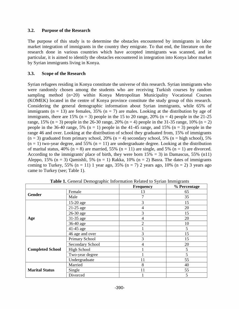
-390-

3.2. Purpose of the Research

The purpose of this study is to determine the obstacles encountered by immigrants in labor

market integration of immigrants in the country they emigrate. To that end, the literature on the

research done in various countries which have accepted immigrants was scanned, and in

particular, it is aimed to identify the obstacles encountered in integration into Konya labor market

by Syrian immigrants living in Konya.

3.3. Scope of the Research

Syrian refugees residing in Konya constitute the universe of this research. Syrian immigrants who

were randomly chosen among the students who are receiving Turkish courses by random

sampling method (n=20) within Konya Metropolitan Municipality Vocational Courses

(KOMEK) located in the centre of Konya province constitute the study group of this research.

Considering the general demographic information about Syrian immigrants, while 65% of

immigrants (n = 13) are females, 35% (n = 7) are males. Looking at the distribution by age of

immigrants, there are 15% (n = 3) people in the 15 to 20 range, 20% (n = 4) people in the 21-25

range, 15% (n = 3) people in the 26-30 range, 20% (n = 4) people in the 31-35 range, 10% (n = 2)

people in the 36-40 range, 5% (n = 1) people in the 41-45 range, and 15% (n = 3) people in the

range 46 and over. Looking at the distribution of school they graduated from, 15% of immigrants

(n = 3) graduated from primary school, 20% (n = 4) secondary school, 5% (n = high school), 5%

(n = 1) two-year degree, and 55% (n = 11) are undergraduate degree. Looking at the distribution

of marital status, 40% (n = 8) are married, 55% (n = 11) are single, and 5% (n = 1) are divorced.

According to the immigrants' place of birth, they were born 15% = 3) in Damascus, 55% (n11)

Aleppo, 15% (n = 3) Qamishli, 5% (n = 1) Rakka, 10% (n = 2) Basra. The dates of immigrants

coming to Turkey, 55% (n = 11) 1 year ago, 35% (n = 7) 2 years ago, 10% (n = 2) 3 years ago

came to Turkey (see; Table 1).

Table 1. General Demographic Information Related to Syrian Immigrants Frequency % Percentage

Gender Female 13 65

Male 7 35

Age

15-20 age 3 15

21-25 age 4 20

26-30 age 3 15

31-35 age 4 20

36-40 age 2 10

41-45 age 1 5

46 age and over 3 15

Completed School

Primary School 3 15

Secondary School 4 20

High School 1 5

Two-year degree 1 5

Undergraduate 11 55

Marital Status

Married 8 40

Single 11 55

Divorced 1 5

-391-

Place of Birth

Damascus 3 15

Aleppo 11 55

Qamishli 3 15

Rakka 1 5

Basra 2 10

Date of Arrival in

Turkey

1 year ago 11 55

2 years ago 7 35

3 years ago 2 10

When examining Syrian immigrants' demographic information relating to the labor market, 25%

of immigrants (n = 5) are teachers, 5% (n = 1) are ironworkers, 5% (n = 1) are fashion designers,

5% (n = 1) are house painters, 5% (n = 1) are builders, 5% (n = 1) are home decorators, 10% (n =

2) are students, 5% (n = 1) are physiotherapists, 5% (n = 1) are accountants, 5% (n = 1) are

hairdressers, 5% (n = 1) are Veterinaries, and 20% (n = 4) do not have professions. Considering

the situation of Syrian refugees in Turkey to practice their professions, while only 25% (n = 5) of

them can perform their professions, 75% (n = 15) cannot. When we look at the distribution of

migrants according to their employment status, while 45% (n = 9) are working, 55% (n = 11) do

not have jobs. Their monthly income is 20% (n = 4) are in the range 500-1000 Turkish Lira-

TL(163$-326$), 25% (n = 5) are 1.000-1.500 TL(326$-489$) (range, and 55% (n = 11) do not

have regular incomes (See. Table 2).

Table 2. Syrian Immigrants' Demographic Information Related to Labor Force Frequency % Percentage

Profession

Teacher 5 25

Ironworker 1 5

Fashion Designer 1 5

House Painter 1 5

Builder 1 5

Home Decoration 1 5

Student 2 10

Physiotherapist 1 5

Accountant 1 5

Hairdresser 1 5

Veterinary 1 5

Doesn’t have a profession 4 20

Can They Practice the

Profession in Turkey?

Yes 5 25

No 15 75

Do They work in Any

Jobs?

Yes 9 45

No 11 55

Monthly Income

500-1.000TL (163$-326$) 4 20

1.000-1.500TL (326$-489$) 5 25

Has no regular income 11 55

The reason for coming

to Turkey

Safety / Safety of Life 6 30

War 10 50

Economy / Unemployment 4 20

-392-

3.4. Method of the Research

Qualitative data related to this study was collected through a semi-structured interview form

developed by the researcher from the interviews with Syrian immigrants (n = 20) going to

KOMEK Turkish learning course located in the centre of Konya province in January 2016. The

interviews were held with the immigrants who voluntarily accepted to be interviewed (n = 20),

these interviews were implemented with the questions prepared and developed by the researcher

for the purpose of the study. During this study, the following 2 questions prepared and developed

by the researcher for the purpose of the study were asked to the Syrian immigrants.

1- What are the main problems you encounter while working in the business

environment?

2- What are the main problems you faced while finding a job?

Qualitative data obtained during this research was obtained by the researcher using the semi-

structured interview technique from the qualitative research techniques. The reason to use the

interview method during this research is to try to gather information listening to the immigrants

as the primary source on the subject. Because of language problems, assistance was received

from the KOMEK Turkish Course lesson teacher for a better understanding of the questions.

During the analysis of qualitative data related to the research, content analysis and comparison

techniques were used the by researcher constantly. According to what Merriam (1998) stated, all

qualitative data analysis processes actually mean content analysis. The data obtained from

interviews was compared with the literature on the subject area, and it was checked for accuracy.

Later, the interviews were conducted with the immigrants subject to the research in the

framework of the plan. The data obtained from interviews were compared with the literature

about the subject area again.

4. RESEARCH FINDINGS

According to the findings, the most important obstacles encountered by Syrian immigrants in the

integration into the labor market can be said as being worked for lower wages than they deserve,

and experiencing the state of being unpaid, their exploitation by employers working in harsh

conditions, the lack of continuity and safety at work, their humiliation in the working

environment, encountering difficulties because they do not know the Turkish language, and

experiencing the case of getting unskilled because they do not have the opportunity to practice

their professions. The views of the Syrian immigrants who participated in this study about the

obstacles they face in the labor market participation were given in details below.

When the answeres given to the question "What are the main problems you encounter while

working in the business environment?" were analysed;

- 10 of the immigrants stated that they do not receive equal wages to Turkish employees, they are

worked for lower wages than they deserve, and sometimes they are not paid by their employers.

The views of immigrants in this regard are as follows:

-393-

V1: "I have been working for 3 months. Other employees' wages have increased, I am going on

as I was. While the transportation cost was paid until last month, now they do not pay it. The

employers' behaviors are good. I take care of 5 persons with my salary."

V3:"The working environment, human relations are good. While the Turks are paid more, I am

paid less."

V4:” I am employed for a low wage. It is not equal to the other employees.”

V8:” I want to assist my family but I don't think I will be able to get what I deserve. I worked as

an apprentice in a welder's close to my house. I left two months later. I earned 20 TL (6,5$) or 5

TL (1,6 $) in a day depending on the job.”

- Those who think that they were exploited by the employers employed under more pressure, in

difficult conditions, uninsured, in the lack of safety conditions are 4. The views of immigrants in

this regard are as follows:

V6:” Turkish workers are taking more wages. Our job is dangerous, but no insurance. The way

of adressing is not appropriate; they call as "Syrian! Come here!" A piece of iron hit on my head,

but they did not take me to hospital.”

V7:” The boss does not treat us well. I am working at a difficult job, but the Turk came to my

place is paid more than me. Our job is dangerous, but we do not have insurance.”

V18:” The employers' behaviours to us are different, there is more pressure, and we cannot get

what we deserve. They pay half salary or they do not pay at all.”

- Those who think that they do not have a guarantee in the sense of continuity of work are 3

people. The views of immigrants in this regard are as follows:

V13:” There is no occupational safety and continuity. I cannot get my salary from UNICEF. In

addition, my students cannot get diplomas.”

V2: “I receive 100TL (32,6 $) weekly, payment is not made, they make me wait. I work overtime.

I cannot communicate with my colleagues because I don't know Turkish. There is no

occupational safety. They promise bu they do not make an increasement.”

- Those who were humiliated by being exposed to ill-treatment by the employer in the workplace

are 2 people. The views of immigrants in this regard are as follows:

V6:” Turkish workers are taking more wages. Our job is dangerous, but no insurance. The way

of adressing is not appropriate; they call as "Syrian! Come here!" A piece of iron hit on my head,

but they did not take me to hospital.”

V7:” The boss does not treat us well. I am working at a difficult job, but the Turk came to my

place is paid more than me. Our job is dangerous, but we do not have insurance”

-394-

- Those who have experienced difficulties because they do not know the Turkish language are 2


V16:” I would like to teach, but I do not dare because I do not know the language. I could get my

diploma recently because of the war.”

- Those who can't practice their own profession and who think that they are being unskilled are 2


V15:” I am an English teacher, but I'm working as a classroom teacher. I would like to work in

my own field.”

V20:” I cannot find a job as a veterinarian. I was offered jobs as sweet manufacturing and so on,

but I did not accept. Salary is too low.”

When the responses of Syrian immigrants to the question "What are the main challenges you

are facing while finding a job?" were analyzed;

- 5 immigrants think that they are to be exploited by employers with low wages being employed

in harsh works:

V3:” I cannot find a job related to my own profession. I couldn't get my payment when I worked

for short times. I feel being exploited about payment. We couldn't get the deposit we had given

the realtor, they didn't provide us with the house, we complained about them.”

V5:” They employ us with low wages. They employ us at heavy work, they abuse us, they

humiliate us. I do not want to work for/with someone else. I want to work as a teacher.”

V7:” I am working for a low wage. It is more difficult to find a job in winter. I couldn't get what I

had worked for, they didn't give me 500TL (163$) that I deserved.”

V8:” Sometimes I couldn't get what I deserved for my work. Sometimes I couldn't get it at all. I

wish to work at a good job, I would like both to work and finish my school.”

V9:” Wages are too low. Sometimes associations and the municipality come home for

reconnoitring. They cut they aid saying that I pay 500TL(163$) for the rent. When they see a

bachelor Syrian girl, they want to marry her directly, but they don't want civil marriage. The

municipality take our aid card saying that there are two people working at home. However, 5

people are working at some homes, but their cards are not taken.”

- Those who think that they will not find a job in which they can practice their own professions

are 3 people. The views of immigrants in this regard are as follows:

V4:” I cannot practice my own profession. I'm having trouble in finding rental housing. We

encounter prejudices.”

V11:” I do not have a graduation diploma. I'm not able to get my diploma from Syria.

-395-

If I can, I can work. I would like to do my profession, but it seems difficult. Syrians are not given

houses. Rents are high. My father was the boss at work, he was also a foreman, but they

employed him like a peon here. When they noticed that he is a foreman, they promopted him but

his salary remained the same, he takes 1.500TL. (489$)”

- Those who do not want to work with someone with the thought that they will be humiliated are

2 people. The views of immigrants in this regard are as follows:

V5:” They employ us with low wages. They employ us at heavy work, they abuse us, they

humiliate us. I do not want to work for/with someone else.”

V9:” Some people look down on us. In fact, our lives in Syria are surperior than theirs.”

- Those who said that they have difficulties in finding a job because they do not know Turkish are

2 people. The views of immigrants in this regard are as follows:

V12:” My goal is to continue my school after learning Turkish.”

V15:” There is no job guarantee. I find it difficult to communicate because I don't know

Turkish.”

In summary, evaluating the findings above; it can be stated that Syrian immigrants receive less

wages compared to Turkish workers, they work under more difficult circumstances, they do now

receive their wages in some cases, they lack the job security and continuity, they have difficulties

because of not knowing Turkish language in the business environment in which they work. It is

noteworthy that unemployed Syrian immigrants do not want to work at hard works for low

wages, they cannot practice their own professions, they don't want to be humiliated in the work

environment, and they cannot speak Turkish language.

5. CONCLUSIONS AND RECOMMENDATIONS

It is observed that the obstacles in integration into the labor market immigrants face in different

countries of the world are largely similar to the obstacles they face in the labor market

participation in Turkey and in Konya province in particular. These are mainly that they can't

speak the language they live in, the possibility of finding jobs in difficult conditions requiring

more labor and working hours with loew wages compared to locals, the lack of security and

continuity in their work, they are not able to reflect the personal qualities they have, and

inadequate legal regulations that make it difficult for their participation into labor market.

When the responses Syrian immigrants gave to the question "What are the main problems you

encounter while working in working environment?" are examined, under the qualitative study in

Konya province intended for identifying the obstacles Syrian immigrants encounter in their

integration into the labor market, most of the immigrants (10 of them) stated that they

experienced being employed for lower wages than they deserve and non-payment of wages. The

conditions of employment based on low wages such as agriculture, construction, storage

experienced in labor-intensive areas in Karaca and Doğan's study (2014) have the qualities that

support our findings. In addition, forcing Syrians to work for a low wage, and non-payment of

-396-

wages after work, the police station's requirement for a certified interpreter when they are

directed to the police station, and the interpreter's demand for 100TL (32,6$) for interpretation,

Syrians' fear of the police, the fear of deportation, and being unable to ask for their rights because

they don't have money (Karaca and Doğan, 2014) also support the obtained results. Besides,

Ulukan's view (2008) that "Immigrants often face with unemployment in the labor market, they

are obliged to accept low-paid and unskilled jobs in order to maintain their lives." supports our

findings.

Those who think that they will be exploited by being worked in harsh conditions are one-fifth of

the immigrants (4 people). Akpinar stated (2009) that immigrant workers are worked long hours

during the day by force if necessary. Because there are a large number of illegal migrant workers

wandering around unemployed, these put pressure on those who are received to work. Hired

immigrant workers are laid off after work for 1-2 months, and the post is filled with new one

immediately. The view that "the employers mainly short-change these workers who they make

them work long hours during the day and harsh work, and sometimes they do no payment at all"

supports our findings.

Those who think that there is no continuity and safety at work are 3 people. The precarious, lack

of job security, non-permanent (seasonal) employment conditions that are experienced in labor-

intensive areas support our findings.

Those who think that they are humiliated in the working environment are 2 people. Dedeoglu's

view (2011) that "Azerbaijani immigrant women and children are socially excluded, and they are

sometimes exposed to physical and verbal violence, their migration experience and social

exclusion influence not only adult immigrants but also the new growing generation, exclusion

from education and health services increase the risk of being faced with poverty and social

exclusion for the more needy children to these facilities" is in line with our findings.

Those who think that they have difficulties because they do not know Turkish language are 2

people. Chiswick (1978) described immigrants' knowing the language of the country they

emigrate as human capital, in addition, the views that "as cultural and linguistic differences

among the natives and immigrants decrease, as they learn the language, differences in economic

opportunities will disappear over time" are parallel to our findings. (Cited by Portes and Zhou,

1992)

Those who think that they are getting unskilled through being unable to practice their own

professions are 2 people. Ekiz-Gökmen's (2011) view that "being employed out of the training

they have received and the quality they own cause immigrant women to be unskilled, causing

educated immigrant women to be unskilled through being employed in low-skilled jobs with low

wages is the most important problem they experience in the market." supports our findings.

The answers given to the question "What are the main problems you encounter while finding

work?", most of the immigrants (5 of them) think that they will be exploited by the employer

through being employed with low wages. According to Ulukan (2008), although low-paid work

seems to be the survival strategy of immigrants, being obliged of Syrians to work with little

wages and non-payment of wages after working raise the idea of not working in the present

circumstances in some immigrants.

-397-

Those who think that they will not be able to find a job related to their professions are 3 people.

The reason for this opinion is that their diplomas they received in their country are not valid in

Turkey. Those who do not want to work for someone else with the opinion of being humiliated

are 2 people. This view has come to the fore for those who have a certain social status in Syria,

and have better financial opportunities. Those who say that they have difficulties in finding a job

because of not knowing Turkish are 2 people. The ones who have this view think that KOMEK

Turkish course will be useful to address this shortcoming of them.

In order to ensure a higher rate of integration of Syrian immigrants into the labor market, it is

evaluated that;

- Beside the continuation of Turkish courses providing continuity, in particular, giving training

for acquiring professional skills in order to find employment opportunities in manufacturing and

in fields not requiring much expertise,

- Encouraging employers in order to be employ them in the open jobs in the manufacturing sector

in Konya,

- Taking measure for employment in the agricultural sector in which a decline has been

experienced in recent years in Konya,

- Making arrangements for those who can present graduation and training documents to do their

professions,

- It would be useful to audit employers on job security and abuse issues.

RESOURCES

1. Abowd, J. M., Freeman, R. B. (1991). Immigration, Trade, and the Labor Market. Chicago and London:

The University of Chicago Press

2. Akpınar, T. (2009). Türkiye’ye Yönelik Düzensiz Göçler ve Göçmenlerin İnşaat Sektöründe Enformel

İstihdamı. Yayınlanmamış Doktora Tezi, Ankara Üniversitesi Sosyal Bilimler Enstitüsü, Ankara.

3. Brenke, K. (2015). Distribution of refugees very uneven among EU member states -even when accounting

for economic strength and total population. DIW Economic Bulletin, 39, 511-523.

4. Chiswick, B. R. ( 1978). The Effect of Americanization on the Earnings of Foreign-Born Men. Journal of

Political Economy, 86(5), 898.

5. Çolak, Ö. F. (2010). Küresel İstihdam Sorunu. Ankara: Efil Yayın Evi

-398-

6. Dedeoğlu, S. (2011). Türkiye’de Göçmenlerin Sosyal Dışlanması: İstanbul Hazır-Giyim Sanayinde

Çalışan Azerbaycanlı Göçmen Kadınlar Örneği. Ankara Üniversitesi SBF Dergisi, 66(1): 26-48.

7. Ekiz-Gökmen, Ç. (2011). Türk Turizminin Yabancı Gelinleri: Marmaris Yöresinde Turizm Sektöründe

Çalışan Göçmen Kadınlar. Çalışma ve Toplum, 1, 200-231.

8. Erdoğan, M. (2014). Türkiye’deki Suriyeliler: Toplumsal Kabul ve Uyum Araştırması. Hacettepe

Üniversitesi Göç ve Siyasi Araştırmalar Merkezi Raporu.

9. Fratzscher, M., Junker, S. (2015). Integrating Refugees: A long-term, Worthwhile Investment. DIW

Economic Bulletin, 45, 612-616.

10. Germir, H. N. (2012). Türkiye İstihdam Politikalarının Etkinliği. Ankara: Adalet Yayınevi.

11. Karaca, S., Doğan, U. (2014). Suriyeli Göçmenlerin Sorunları Çalıştayı Sonuç Raporu. Mersin

Üniversitesi Bölgesel İzleme Uygulama Araştırma Merkezi.

12. Kömürcü, E. (2011). Almanya’da Yaşayan Türk Göçmenlerin Sosyo-Kültürel Sorunları: Bir Entegrasyon

Çalışması. Yayınlanmamış Yüksek Lisans Tezi, Ankara Üniversitesi Fen Bilimleri Enstitüsü, Ankara.

13. Lewis, T. (2015). Explaining the (Non-)Encampment of Syrian Refugees: Security, Class and the Labour

Market in Lebanon and Jordan, Mediterranean Politics, 20(3): 386-404.

14. Man, F. (2015). Some reflections on migration and its effects on host Country’s labour market: Syrian

refugees in Turkey. Proceedings of the Multidisciplinary Academic Conference. October, 1-9.

15. Merriam, B. S. (1998). Qualitative Research and Case Study Applications in Education. San Francisco:

Jossey Bass Publishers, 2.

16. Portes, A., Zhou, M. (1992). Gaining the Upper Hand: Economic Mobility Among Immigrant and

Domestic Minorities. Ethnic and Racial Studies, 15(4) :493.

17. Tunç, A. Ş. (2015). Mülteci Davranışı ve Toplumsal Etkileri: Türkiye’deki Suriyelilere İlişkin Bir

Değerlendirme. Tesam Akademi Dergisi, 2 (2): 29-63.

18. Ulukan, N. C. (2008). Göçmenler ve İşgücü Piyasası: Bursa’da Bulgaristan Göçmenleri Örneği.

Yayınlanmamış Doktora Tezi, Marmara Üniversitesi Sosyal Bilimler Enstitüsü, İstanbul.

-399-

19. Uslu, L. (2012). Göçmenlerde Yoksulluk Yansımalar Denizli Örneği. Yayınlanmamış Yüksek Lisans Tezi,

Pamukkale Üniversitesi Sosyal Bilimler Enstitüsü, Denizli.

20. Ünlütürk- Ulutaş, Ç. (2013). Almanya’yı Temizliyorum: Almanya’da Göçmen, Kadın ve Temizlikçi

Olmak, Çalışma ve Toplum, 2, 235-257.

21. Yavuz, A. (2012). İşgücü, İstihdam ve Kriz Olgusu. İstanbul: İTO Yayınları.

22. http://www.tuik.gov.tr/PreHaberBultenleri.do?id=18644 (Access Date: 15 December 2015)

23. Internet References:

24. http://www.tuik.gov.tr/jsp/duyuru/upload/yayinrapor/HIA_2013.pdf TÜİK Hane Halkı İş Gücü

Araştırması Bölgesel Sonuçlar 2004-2013 (Access Date: 10 December 2015)

25. http://www.konyadayatirim.gov.tr/images/dosya/2015_KONYA_%C4%B0%C5%9EG%C3%9CC%C3%9C_P

%C4%B0YASASI_TALEP_ARA%C5%9ETIRMASI_RAPORU.pdf (Access Date: 25 December 2015)

26. http://www.goc.gov.tr/icerik3/gecici-koruma_363_378_4713 (Access Date: 20 January 2016)

27. http://www.mevzuat.gov.tr/MevzuatMetin/3.5.20168375.pdf (Access Date: 15 December 2015)

http://www.tuik.gov.tr/jsp/duyuru/upload/yayinrapor/HIA_2013.pdf

http://www.konyadayatirim.gov.tr/images/dosya/2015_KONYA_%C4%B0%C5%9EG%C3%9CC%C3%9C_P%C4%B0YASASI_TALEP_ARA%C5%9ETIRMASI_RAPORU.pdf%20(Erişim

http://www.konyadayatirim.gov.tr/images/dosya/2015_KONYA_%C4%B0%C5%9EG%C3%9CC%C3%9C_P%C4%B0YASASI_TALEP_ARA%C5%9ETIRMASI_RAPORU.pdf%20(Erişim

http://www.goc.gov.tr/icerik3/gecici-koruma_363_378_4713%20(

-400-

HEDGING OIL PRICE RISK BETWEEN OIL IMPORTER AND OIL EXPORTER

COUNTRIES A CASE STUDY FOR TURKEY AND MEXICO

Nadir Eroğlu


İmran Emre Karagözlü


Ahmet Akca

Bahçşehir University, Turkey

Abstract

Substantial and unpredictable movements in oil prices could harm the macroeconomic

performance of oil exporting and importing countries. Some countries try to take precautions

against this exposure, yet solutions have not proliferated. This paper tries to propose a mitigation

solution to the adverse effects of volatility in oil market. In this regard, macroeconomic effects of

oil price changes on oil exporting and importing countries are outlined first. Then, a bilateral

contract between Mexico and Turkey, two oil trading countries, is drafted. The hedge model in

this contract is composed of a couple of different hedge strategies which are valued via Monte

Carlo simulations. The performance of proposed hedge strategies with respect to the government

revenues and expenditures are calculated through three years. Results show that zero-cost collar

strategy might serve as an effective protection against oil price fluctuations for both countries.

Keywords: Hedging, Oil Price Risk, Monte Carlo Simulation

I. IMPORTANCE OF OIL PRICE RISK FOR OIL EXPORTING AND OIL IMPORTING

COUNTRIES

Macroeconomic performance of oil importing and exporting countries depends significantly on

the changes of oil prices worldwide. Economic growth, foreign exchange rates, interest rates,

budget deficit and current account deficit which could be referred to as Macroeconomic Key

Performance Indicators - KPIs have tended to fluctuate during the periods in which oil prices

were volatile. Recent volatility in oil markets, once again, triggered concerns about the impact of

oil price shocks on Macroeconomic KPIs around the world. In this section, importance of oil

price volatility for oil exporting and oil importing countries will be analyzed. Turkey, a major oil

importing country, has exogenous dependency in energy sector and upward fluctuations in oil

price has adverse impact on Turkish economy. On the other hand, Mexico, a major oil exporter,

will benefit from such a move. However, the reverse movement of the price will affect these

countries the other way around. Changes in oil prices lead to significant real income shifts among

oil exporters and oil importers suggesting that when the oil prices do not remain stable, at least

one of the counterparty will gain at the expense of the other. [1]

In this context, Turkish economy and its vulnerabilities will be examined in line with oil price

movements. Turkey is a developing country with total energy consumption of around 130 million

-401-

tones oil equivalent. GDP of Turkey is $735 billion and energy consumption is $26 billion. This

means, with current crude oil prices (Brent $45/barrel), Turkey’s energy expenditure is at its

lowest with 4% of GDP since 2000s. Figure 1 shows how the oil price and total energy bill of

Turkey behave concurrently. Figure 2 provides Pearson correlation results of ICE Brent yearly

price averages (Y – axis) and Turkey’s energy bill (X – axis). With an R score of 0.9739, there

seems a significant positive relationship between price of oil and Turkey’s energy bill. [2] Effects

of oil price changes on GDP, current account deficit and interest & foreign exchange markets of

Turkey are in order next.

First, high correlation between oil price and energy bill suggests that a rise in oil prices will

increase Turkey’s energy bill. As suggested in [3], increase in energy bill will potentially cause a

decline in GDP growth. More specifically, lower oil prices improve household real incomes and

non-oil corporate profits. This leads to increase in aggregate demand for consumer products.

Decline in oil prices also relaxes the government budget. Hence, with lower oil prices, public and

private sector will contribute the growth positively. On the other hand, higher prices in energy

market increase energy bills of private and public sectors leading these parties to spend lower.

While there are other variables that affect the growth in the long run, in the short run oil price

increase has a negative effect on growth rates.[4] Interdependency of oil price and GDP can also

be explained via transmission mechanism operating on two channels, namely demand and supply.

From demand side, an unexpected increase in the price of imported crude oil reduces purchasing

power of domestic households and the local income is being transferred to abroad. This causes a

decline in aggregate demand. From supply side, during oil price increases, cost of production

increases and hence aggregate supply shifts left. [5] In sum, during an oil price increase period,

both the demand and supply decline and hence the growth of GDP suffers.

Second, Turkey’s total imports including energy expenditures are higher than the total exports,

which cause Turkey to experience a deficit in current account balance. Due to the this structural

difference, Turkey is exposed to current account deficit increases during oil price hikes.

Third, with high oil prices and current account deficit, demand for foreign exchange to finance

deficit increases. This causes TRY to depreciate and interest rates to increase. Mexico is a

developing country with $1.2 trillion GDP and its oil production is 100 million tones. Mexico

have traditionally funded more than one third of the government’s spending by oil exports but

with the declining oil prices and structural reforms, oil’s contribution to government budget

dropped to 20% which is still high enough to consider its effects. The dramatic declines in oil

prices may have disruptive effects on growth, interest rates and foreign exchange currency as

explained in [6]. The loss in oil revenues can strain government budget, and hence necessitate

spending cuts or external borrowing.

-402-

0,0

20,0

40,0

60,0

80,0

100,0

120,0

ICE Brent Average ($/bbl) Turkey Energy Bill (bio,$)

Fig. 1. ICE Brent Yearly Average Price /

Turkey Energy Bill Amount


Turkey Energy Bill Amount - Pearson

Correlation

0,0

20,0

40,0

60,0

80,0

100,0

120,0

ICE Brent Average ($/bbl) Mexico Oil Revenue (bio,$)


Mexico’s Exports


Mexico’s Exports – Pearson Correlation

First, in case of spending cuts, government may increase taxes or decrease government spending

which will increase the burden on economy. New tax rates or low public demand will affect the

growth rate negatively. A price increase, conversely, will affect the economy via a transmission

mechanism as follows. An oil price increase leads a wealth effect through revenue boost. Public

and private parties consume more tradable and non-tradable products thanks to the income

increase. On the other hand, increased consumption generates a scarcity of non-tradable goods

and this boosts the price of non-tradable goods. According to these two channels, an oil price

increase affect growth positively.

Second, in case of external borrowing, the cost of borrowing in low oil price market will be

higher than the one in high oil price market. Financial institutions will charge extra spread due to

the oil revenue loss. The cost of funding will increase not only for the government but also for all

of the institutions in Mexico. Moreover, increase in interest rates, private investments and

consumptions will decline which will result in a reduction in growth rate.

Third, in addition to the effects on growth and interest rate, declining oil revenue may cause

depreciation in Mexico Peso. The decline in foreign exchange revenue will deteriorate the

balance of payments and economy will require more foreign exchange reserves in low oil

revenue times.

Figure 3 shows how the oil price and total exports of Mexico behave concurrently. Figure 4

provides Pearson correlation results of ICE Brent yearly price averages (Y – axis) and Mexico’s

-403-

exports (X – axis). With an R score of 0.9610, there seems a significant positive relationship

between price of oil and Mexico’s exports. [7]

II. BILATERAL CONTRACT BETWEEN TURKEY AND MEXICO - A SOLUTION

PROPOSAL

We believe that macroeconomic performance of both countries can simultaneously be improved

regardless of the level of the volatility in the price of oil provided that a contract taking both the

trade and risk management dynamics into account and ensuring better terms than those of risk

market.

Such a contract can be superior to managing these risks in the risk markets individually since in

the latter case, the country has to manage the market volume risk, financial cost of contract,

counterparty risks and political risks separately. The contract between these countries provides a

solution basically with real trade market, and this limits the risks of derivative markets which

may disconnect from the real economy substantially.

In this study, a contract between these two countries is proposed in terms of the underlying asset,

maturity, hedging instruments and hedging strategies.

• Underlying Asset: The ICE Brent Crude is the underlying asset due to the

depth of volume, correlation with the abovementioned KPIs and availability of

transparent price. Price of the underlying asset, ICE Brent Crude, is the average of

relevant month.

• Hedging Maturity: At the inception, next 24 months will be fully hedged

with monthly hedge contracts. Then, for the first year, at the end of each month,

third year’s exposure will be hedged monthly. In other words, first two years are

hedged at the inception, and last year is hedged throughout the first year, making a

total of three-years hedging period.

• Hedging Instruments and Strategies: No-Hedge strategy is the base (as is)

case in which Turkey and Mexico will separately be exposed to market price

changes. Second strategy fully hedges both exposures of both countries with

futures priced via the model. Third strategy uses zero cost collar structures for full

hedge.

Oil export revenue for Mexico and energy bill for Turkey are the variables on which the effects

of proposed hedge strategies will be analyzed as a proxy for Macroeconomic KPIs defined in

above sections.

III. HEDGE MODEL

Underlying asset have long followed a mean-reversion pattern from 1994 to 2000s but it changes

to a Brownian motion process as of then as discussed in [8]. Hence, the model in this study is

built on Brownian motion pattern. To this end, underlying asset follows below process:

dSt = µSt dt + σSt dWt (1)

The solution to this Stochastic Differential Equation (SDE) is given by:

(2)

-404-

To generate asset prices, a path-dependent Monte Carlo simulation with 5,000 trials has been

performed. In the simulation, daily prices are generated with following data:

• rf = 1.59%

• σ= 28.50%

• S0 = $45 per barrel

• t = 1 days and T = 3 years

• Convenience Yield= 0

• Number of trials= 5; 000

For each month, 22 business days were assumed, hence in total prices for 792 business days for 3

years were calculated in each trial. Monthly averages were used to calculate collar structures

consisting of call and put options with strikes generating zero-cost premiums. Future prices, on

the other hand, are calculated based on:

Ft = S0erf dt (3)

Given the simulation results, we have 36 monthly average prices of underlying asset, 36 zero-cost

strategies, 36 future prices. These provide us with payout structures of no hedge, zero-cost collar,

and future strategies. Payouts of these three strategies are calculated for the highest, lowest and

mean price scenarios with respect to model-generated spot prices. The highest (lowest) price

scenarios are formed by taking the highest (lowest) sum of 10 paths out of 5,000 trials. Mean

price scenarios are formed in a similar manner. The aim to carve out these price scenarios is to

demonstrate the effects of extreme cases on the Macroeconomic KPIs of both countries.

IV. RESULTS

As described above, the highest, lowest and mean prices generated via Monte Carlo for ICE

Brent Crude is displayed in Figure 5. According to these results, last year (3rd year) averages of

the highest, lowest and mean asset prices are $111.5, $22.1, $51.6 per barrel, respectively.

0

20

40

60

80

100

120

ICE Brent Average ($/bbl) High Mean Low Futures

Fig. 5. ICE Brent Crude Yearly Average Prices

Instead of calculating cash-settle P&Ls for both countries in each strategy, we have directly

shown the effects of the final strategy price on the Macroeconomic KPIs as the prices to be born

in each strategy is the final price of purchasing (for Turkey) and selling (for Mexico). To be able

to determine the level of Macroeconomic KPIs with each final strategy price, we need to estimate

how the relevant indicators will behave.

-405-

To achieve this, regression analysis were performed. More specifically, energy bill of Turkey and

oil export revenue of Mexico were regressed over Brent prices separately. The results of the

regressions are as follows. Both regressions produce almost zero p – values, implying significant

relationship.

Energy Bill of Turkey = -4.25 + 0.55 x ICE Brent

Oil Revenue of Mexico = 4.03 + 0.45 x ICE Brent

With these equations, energy bill of Turkey and oil export revenue of Mexico can now be

estimated under the highest, lowest and mean price scenarios generated by above model for no

hedge, zero-cost collar and future hedge strategies. The results of these strategies for Turkey and

Mexico are given in Figures 6 & 7, Figures 8 & 9, respectively. As seen in the graphs, no hedge

strategy exposes both countries to effects of volatile oil prices. On the other hand, future hedge

strategy eliminates all the effects of volatility whereas zero-cost collar strategies provide a range

whereby both countries can benefit from market movements upto strike levels and locks-in the

strike level prices for the rest of price scenarios. Compared with futures hedge strategy, zero-cost

collar strategy seems better fitting as it provides some room to benefit from market movements to

both countries.

Fig. 6. No Hedge Strategy Results for

Turkey’s Energy Bill

Fig. 7. Zero-Cost Collar and Futures

Strategy Results for Turkey’s Energy Bill

Fig. 8. No Hedge Strategy Results for

Mexico’s Oil Export Revenue

Fig. 9. Zero-Cost Collar and Futures

Strategy Results for Mexico’s Oil Export

Revenue

-406-

V. CONCLUSIONS AND RECOMMENDATIONS FOR FUTURE STUDIES

In this study, effects of oil price on macroeconomic performances of Turkey and Mexico are

analyzed. Since macroeconomic performance of both countries are dependent heavily on oil

price, volatility in the price of oil may deteriorate economic performance of the countries if

unhedged.

To understand the effects of hedging oil price risk, a bilateral contract of a specific nature has

been proposed. Monte Carlo simulation was used to price different hedge strategies and

regression analysis were used to calculate the payout effects of hedge strategies on the

Macroeconomic KPIs of both countries. The results suggest that both countries can benefit from

zero-cost collar hedge strategies. Hedges will be put in place immediately at the inception for the

first 2 years on monthly basis, and then will gradually be extended on a monthly basis to 3rd year

during the first year.

Recommendations for future studies are outlined below:

• Pricing of the underlying is done with Brownian motion. For future studies, this

method can be scrutinized by comparing with mean-reverting process.

• In this study, strikes levels of call and put options in zero-cost collars are near at

the money (ATM) levels for all of 3 years. Strike levels can be adjusted to better reflect

budget sensitivities of both countries. For example, range of the strike levels may be

widened for each of the following 2nd and 3rd year. In the event that oil prices

successively increase (decline) as opposed to oscillating, call (put) option will start and

continue to work and exporting (importing) country will find itself in an unwanted

position. A widening strike range, thus, provides both countries with improved market

participation as compared with ATM strike levels in non-oscillating price movements.

Furthermore, widened strikes will ensure sufficient time to execute structural policies

without losing opportunities of market participation. Finally, call and put options in the

zero-cost collar strategies are taken European. To better reflect the risk appetite of two

countries, options with American barriers (kick-in, kick-out levels) might be studied.

• Risk free rate and volatility of the underlying are assumed constant. They could be

stochastically modelled to better fit the changing dynamics of markets.

• Hedges are put in place in full amounts. Expected changes in the composition of

Turkey’s energy mix and Mexico’s revenue structure over 3-year horizon could be

reflected by adjusting the level of hedges.

• Convenience yield is assumed 0. Its effect on the price of the underlying and

hence the hedge strategies could be further analyzed.

• A back-test can be performed to test the viability of the performance of the

contract for both countries.

REFERENCES

1. John Baffes and others, The Great Plunge in Oil Prices: Causes, Consequences, and Policy

Responses, World Bank Policy Research Note, PRN/15/01, March 2015, pp.8-9

2. Turkish Statistical Institute http://www.turkstat.gov.tr/Start.do and Bloomberg Data Terminal,

Ticker: CO1 Comdty (16/11/2016)

-407-

3. Sauter, Raphael, and Shimon Awerbuch. ”Oil price volatility and economic activity: a survey

and literature review.” IEA Research Paper (2003): 2-12.

4. Ayen Edirneligil and Mehmet Mucuk, The Effects of Oil Price on Turkish Economic Growth,

12th International Academic Conference, pp.360-370, Prague, p.369

5. Lutz Kilian, Oil Price Shocks: Causes and Consequences, http://wwwpersonal. umich.edu/

lkilian/arre083113 cepr.pdf, p.10, (19/11/2016)

6. John Baffes and others, Understanding the Plunge in Oil Prices: Sources and Implications,

Global Economic Prospects, pp.155-168, (January 2015), pp.162-163

7. Mexico Statistical Institute http://www.inegi.org.mx/ and Bloomberg Data Terminal, Ticker:

CO1 Comdty (16/11/2016)

8. Geman, Hlyette. ”Mean reversion versus random walk in oil and natural gas prices.”

Advances in Mathematical finance. Birkhuser Boston, 2007. 219-2

http://wwwpersonal/

~ 408 ~

EDUCATION LEVEL AND ECONOMIC GROWTH: THE EUROPEAN EXPERIENCE

Mohammadreza Allahverdian Eastern Mediterranean University, North Cyprus

Mohammad Rajabi Eastern Mediterranean University, North Cyprus

Mohsen Mortazavi Eastern Mediterranean University, North Cyprus

Abstract

This paper tried to investigate the nexus between economic growth and education level of the 14

selected European countries (Austria, Czech Republic, Finland, France, Hungary, Italy, Netherlands,

Norway, Poland, Portugal, Spain, Sweden, Switzerland, and United Kingdom) over the period 1990

through 2013 on the yearly basis by exerting panel unit root tests, panel cointegration, panel fully

modified ordinary least squares (FMOLS), panel dynamic ordinary least squares (DOLS), and panel

causality test. In this paper as dependent variable, GDP has been employed as a gauge of economic

growth. On the other hand, government expenditure on education as well as enrollment of student

(primary and secondary) as measure of education level have been used as independent variables.

Furthermore, capital and labor force have been exerted as control variables. The empirical results of

FMOLS as well as DOLS demonstrate that government expenditure on education as well as number

of enrollment of student have significant positive impact on economic growth. The results of

common coefficient panel causality test determine that the relationship between enrollment and

economic growth is bilateral causality. On the other hand, the findings of individual coefficient panel

causality test depict that economic growth homogeneously causes both government expenditure on

education as well as enrollment of student in uni-directional way.

Keywords: Keywords: Education, economic growth, FMOLS, DOLS, panel causality test

1. Introduction

Amongst a few critical features of the advancement, the most vital role is played by schooling in

a country. Basically, the short term economic objectives of a country is tried to direct by

education short term strategies throughout consciousness project on welfare, environment,

earning revenue, making life’s standards as well as managing family size. However, these aims

in the long term are associated with nation’s productivity factor, advancement in human capital,

growth in economic as well as advancement in socio-economic. Thus, people’s efficiency,

inventiveness, entrepreneurship and technology development is increased by education in some

countries (World bank, 2010). According to Isola and Alani (2012), several developing nations

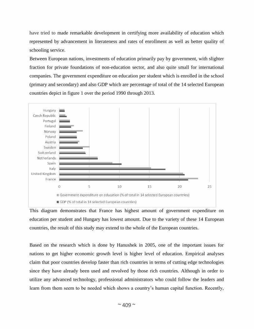
~ 409 ~

have tried to made remarkable development in certifying more availability of education which

represented by advancement in literateness and rates of enrollment as well as better quality of

schooling service.

Between European nations, investments of education primarily pay by government, with slighter

fraction for private foundations of non-education sector, and also quite small for international

companies. The government expenditure on education per student which is enrolled in the school

(primary and secondary) and also GDP which are percentage of total of the 14 selected European

countries depict in figure 1 over the period 1990 through 2013.

This diagram demonstrates that France has highest amount of government expenditure on

education per student and Hungary has lowest amount. Due to the variety of these 14 European

countries, the result of this study may extend to the whole of the European countries.

Based on the research which is done by Hanushek in 2005, one of the important issues for

nations to get higher economic growth level is higher level of education. Empirical analyses

claim that poor countries develop faster than rich countries in terms of cutting edge technologies

since they have already been used and revolved by those rich countries. Although in order to

utilize any advanced technology, professional administrators who could follow the leaders and

learn from them seem to be needed which shows a country’s human capital function. Recently,

~ 410 ~

the critical role of fundamental economic institutions and cognitive skills in the economic growth

has been investigated in some studies. Education has positive relationship with labor force which

results in higher productivity and a stable amount of output in economy. Furthermore, education

has the ability to increase the innovative capacity of the economy through new findings in the

areas such as technology and production, along with simplifying the process of spreading the

latest knowledge of the technologies which leads to promoting growth.

The aim of the current study was to analyze the contribution of education to the economic

growth of the selected European countries. The following purposes are the specific objective

which are consistent with the main objective:

1- Create a relationship between education and GDP

2- Assess the amount of contribution education has on the labor force and capital

3- Investigate whether or not there is an ongoing relationship between education and

economic growth

Since it has proven that education has a positive impact on economic advancement, three

theories regarding this topic are going to be mentioned:

• The basic human capital approach states that overall workforce skills and capability

through education and knowledge which make utilizing the current technology easier and

more accessible and as a result economy will grow.

• The innovation approach claims that education helps establishing new ideas and

technologies

• Knowledge transfer approach also states that education can be a tool to spread the

knowledge in order to use it to create new and innovative technologies.

Even though the correlation between education and economic function has been sated, yet the

causal relation and its direction have not been discovered. It could be the fact that there is no

causality link between these two or economic growth can lead to a better educational

achievement or more educated workforce increase the overall economic function. However, in a

study by Patron and Vaillant (2012), it was claimed that the ratio of skilled-to-unskilled labor

stock is considered as an essential factor to a stable economic growth.

~ 411 ~


In general, education and economic performance seem to be correlated. The firms can benefit

from new economic opportunities through skilled forces which results in better economic

performance and on the other side improved economic brings more educational resources.

Furthermore, although the link between government expenditure and economic growth has been

widely investigated, however it led to some inconsistency among the researchers. It has been

claimed that government expenditure has a positive effect on economic growth. For example,

Bhunia (2012) revealed that such an effect is through providing more facilities and equipment

and services to schools. However, some other authors believe in a negative correlation between

economic growth and government expenditure on education. In one study, Saad and Kalakech

(2009) stated that in short-run the relationship between these two is negative but in long-run it is

positive. Dastidar and Chatterji in 2015 in India found a different impact of education

expenditure on economic growth based on education level such as primary, secondary and

tertiary in public schools.

The result of researches in the last decade emphasize that societies need to improve educational

policy to increase more growth. As Hanushek and Woessmann (2007, p.1) defined; “educational

quality – particularly related to developing countries – is the key issue” in such a growth.

Increased quality and quantity are the two main ways that education can be improved. In the

quantity way, the hours of training enhance the different types of school achievements including

reading, mathematics and science. In the quantity way, human capital productivity can be

boosted in the long-run by increasing the quantity of education. In addition, more skilled labors

cause better innovation and as a result improvement in the economy. Hanushek and Woessmann

(2007, p. 24) in their book revealed that education plays a critical role in educating human

capital, paving the way for more advanced research and also spreading the technologies. So

according to Hanushek and Woessmann (2007) Students get more familiar with new

technologies through schooling however they did not believe in any direct link between

development and quantity of education.

Barro (1991) investigated the economic growth in a cross section of countries by using sample of

98 countries over the period 1960 through 1985. The results of his study demonstrate that

enrollment of students in primary school as well as secondary school have significant positive

~ 412 ~

impact on GDP which represent that by increasing number of students in primary and secondary

school level of GDP will go up. In another research which is done by Levine and Renelt (1992)

about a sensitivity analysis of cross country growth regressions there are similar results. They

found out that the enrollment rate of student in primary and secondary schools have significant

positive influence on level of GDP. Mankiw et al., (1992) explored the economic theory to

achieve determinants of economic growth by using annual data of almost all countries over the

period 1960 throughout 1985 retrieved from real national account. The results of their study

show that the rate of enrollment of student in primary and secondary school have significant

impact on growth of GDP by exerting ordinary least squares.

According to preceding literature reviews it has been proved that government expenditure on

education as well as enrollment of students have impact on level of economic. Based on previous

scholars which mentioned above this study tried to investigate the relationship between

economic growth and level of education.

3. Methodology

3.1 Sample of the Study

The data of this paper has been retrieved from World Bank data bank for 14 selected European

Countries over the period 1990 through 2013. This panel data conducts 336 country- year

observation. To achieve the end of this paper Eviews 9 has been employed.

3.2 Model Specification

In this paper five variables have been selected to demonstrate what is the nexus among level of

education and economic growth in 14 selected European countries. Therefore, GDP as the

dependent variable and government expenditure on education as well as enrollment of students

as independent variables have been exerted. In addition, labor force and gross capital formation

have been entered as control variables to avoid biasedness of coefficients. The panel framework

model of this paper is as follow:

LNGDPit = β1 + β2 LNGOVit + β3 LNENRit + β4LN Lit + β5 LNKit + uit

~ 413 ~

Where i changes from 1 to 14 refers to countries, t refers to years from 1990 to 2013, LNGDP is

the natural logarithm of a proxy of economic growth, LNENR is the natural logarithm of number

of students which enrolled in primary and secondary schools, LNLAB is the natural logarithm of

Labor force, LNCAP is the natural logarithm of gross capital formation and u is error term.

3.3 The panel unit root test

For assessing the existence of unit root in univariate time series, the DF (Dicky Fuller) or ADF

(Augmented Dicky Fuller) have been employed traditionally. However, these tests have been

proven to have low power for rejecting the non-stationary under the null hypothesis and limiting

distributions which are complicated and not well defined as well. Because of these disadvantages

lots of attentions have been recently attracted to the investigating about unit root test.

(FMOLS18). Using the information cross sectional will increase the power of the unit root test

(Abuaf and Jorion ,1990). There are different types of tests such as Levin et al. (2002), LLC

hereafter; Dickey and Fuller (1979, 1981), Breitung (2000), Im et al. (2003) (IPS hereafter),

Maddala and Wu (1999) and Choi (2001) showing the use of Phillips and Perron (1988) mixed

by Fisher (1932), and Hadri (2000) which have been used for testing the panel unit root test

which their power is more than unit root tests employed for individual series. In this paper, we

utilized Levin, Lin, Chu (LLC) as common root test and Im, Pesaran, Shin (IPS), Fisher-ADF

and Fisher-PP to determine the order of integration for series in this study.

3.4 The panel cointegration tests

The panel cointegration test is expected to have as the same advantages in power that are

presented as when testing unit roots in panel data. We conducted Pedroni (1999) method in the

panel cointegration test to determine if there is possibility of long-run relationship between labor

force, gross capital formation, government expenditure on education, enrollment in primary and

secondary schools and GDP in their natural logarithm form.

The time series panel regression is regarded by Pedroni (1999) as follow:

it = αi + i t + β1i x1i,t + β2i x2i,t + …+ βMi xMi,t + ui,t

~ 414 ~

where m = 1...M are the number of explanatory variables which are potentially cointegrated; t =

1...T and i = 1...N. By employing the Dicky Fuller or Augmented Dicky Fuller for , it can be

determined whether they are I (0) thereby the cointegration between these variables will be

confirmed. For instance:

ui,t = i ui,t-1 + i,j Δ ui,t-j+vi,t

He develops finite-sample properties and asymptotic distribution of testing statistics to test the

non-cointegration under the null hypothesis in the panel. Heterogeneity is allowed in the tests

among cross sections of the panel, in both the long-run and dynamic cointegration vectors. Two

test types have been suggested by Pedroni. The first one which there are four statistics in it is on

the basis of within group approach. They are panel rho-statistic, panel v-statistic, panel PP-

statistic, and panel ADF-statistic. Under this approach the autoregressive coefficients through

different cross sections are pooled for testing the unit root of estimated errors. The second type

which Pedroni has proposed relies on the properties which are derived from between-group

characteristics, which three statistics are included in this type. They are group PP-statistic, q-

statistic and group ADF-statistic. The average of estimated coefficients which be calculated

individually is the basis of these statistics.

3.3. FMOLS and DOLS

There are a lot of estimators available which include within-group and between-group

estimators. For estimating the panel coefficients, investigators use panel FMOLS and panel

DOLS as the most common techniques. Pedroni between- group overweighs within-group

estimators because of some reasons. Pedroni's (2001) approach is implemented in this article.

Although comparing the accuracy of two tests is subjective, Maeso-Fernandez et al. (2006) noted

“the FMOLS test provides more robust results than the DOLS test because fewer assumptions

are needed”. On the other hand, Ouedraogo (2013), argues that “the DOLS is a more powerful

method with disadvantage of lowering the number of degrees of freedom due to the leads and

lags”.

~ 415 ~

According to Harris and Sollis (2003), to answer the question of whether DOLS or FMOLS is

preferred, the empirical evidences have been conflicting. The type of empirical modelling,

number of variables, amount of data used in the model, etc. matter too much and may play a

crucial role in generating robust outcomes.

3.4. Panel Granger causality tests

Existing cointegration relationships among the variables also empower possibility of a causal

nexus between the variables and their direction. The causality direction can change according to

the test results.


4.1 Panel unit root

For investigating the integration degree of LNGDP, LNCAP, LNENR, LNGOV, and LNLAB

the panel unit root tests have been applied. The table Ⅰ shows the results for unit root test that

associated with the full sample.

Table Ⅰ: Unit root tests

Level First differences

statistics Levin, Lin

& Chu

Fisher-

ADF

Fisher-

PP IPS

Levin, Lin

& Chu

Fisher-

ADF

Fisher-

PP IPS

LNGDP

-0.1794

(0.4288)

37.9876

(0.0986)

14.8246

(0.9802)

-2.0297

(0.0212)

-9.6138*

(0.0000)

96.7152*

(0.0000)

103.443*

(0.0000)

-7.1476*

(0.0000)

0.0913

(0.5364)

5.7890

(1.0000)

6.2518

(1.0000)

3.8544

(0.9999)

-11.4705*

(0.0000)

134.331*

(0.0000)

136.333*

(0.0000)

-9.4258*

(0.0000)

8.2210

(1.0000)

0.4771

(1.0000)

0.4813

(1.0000) -

-11.7075*

(0.0000)

166.886*

(0.0000)

170.031*

(0.0000) -

LNCAP

1.1326

(0.8713)

41.4064

(0.0493)

37.5265

(0.1077)

-1.5850

(0.0565)

-11.1242*

(0.0000)

121.831*

(0.0000)

143.869*

(0.0000)

-8.9108*

(0.0000)

-1.6530

(0.0492)

20.9694

(0.8266)

15.9493

(0.9666)

1.2411

(0.8927)

-11.7137*

(0.0000)

152.676*

(0.0000)

170.246*

(0.0000)

-10.5118

(0.0000)

5.0280

(1.0000)

2.0058

(1.0000)

2.4753

(1.0000) -

-14.4216*

(0.0000)

210.929*

(0.0000)

218.449*

(0.0000) -

LNENR

-2.5480

(0.0054)

22.7362

(0.7461)

21.8758

(0.7870)

-0.1213

(0.5483)

-5.0595*

(0.0000)

73.8537*

(0.0000)

77.3505*

(0.0000)

-5.1531*

(0.0000)

-3.7710

(0.0001)

50.2928

(0.0060)

36.0114

(0.1423)

-0.9981

(0.1591)

-5.6087*

(0.0000)

95.2891*

(0.0000)

91.3100*

(0.0000)

-6.3605*

(0.0000)

0.3573

(0.6396)

39.0768

(0.0797)

44.1827

(0.0266) -

-8.9419*

(0.0000)

144.253*

(0.0000)

137.462*

(0.0000) -

~ 416 ~

LNGOV

-3.0498

(0.0011)

47.3376

(0.0126)

44.9820

(0.0222)

-2.7750

(0.0028)

-11.8429*

(0.0000)

138.628*

(0.0000)

186.381*

(0.0000)

-10.3893*

(0.0000)

-4.2170

(0.0000)

71.3859

(0.0000)

74.9920

(0.0000)

-4.5813

(0.0000)

-14.5420*

(0.0000)

187.099*

(0.0000)

210.963*

(0.0000)

-12.9421*

(0.0000)

1.3694

(0.9146)

10.9417

(0.9984)

12.5470

(0.9947) -

-16.4997*

(0.0000)

268.973*

(0.0000)

282.523*

(0.0000) -

LNLAB

-1.7778

(0.0377)

46.3950

(0.0159)

49.6253

(0.0071)

-0.8760

(0.1905)

-6.9718*

(0.0000)

76.6510*

(0.0000)

89.2765*

(0.0000)

-5.0374*

(0.0000)

-0.7930

(0.2139)

24.0373

(0.6796)

12.8874

(0.9934)

3.7129

(0.9999)

-7.9047*

(0.0000)

93.8609*

(0.0000)

90.4667*

(0.0000)

-6.5405*

(0.0000)

8.7811

(1.0000)

2.2951

(1.0000)

2.4770

(1.0000) -

-6.2664*

(0.0000)

95.5089*

(0.0000)

108.153*

(0.0000) -

Note: (*) indicates that the estimated parameters are significant at the 1% confidence interval. Where refers to

trend plus intercept, refers to intercept, refers to without trend and intercept.

Regarding the results, it can be seen that the unit root is rejected at 1% level under the null

hypothesis for all variables in their first difference whether trend and intercept are included or

not while, it does not happen for them at their level. Hence all variables are integrated to the

order of 1 I (1).

4.2 Panel cointegration test

After having established that LNGDP, LNCAP, LNENR, LNGOV and LNLAB are I (1), authors

proceed to test if there exist a long-run nexus between them by exerting Pedroni’s panel

cointegration technique. The results of the panel cointegration tests are presented in table Ⅱ

which depicted seven various types of statistic that used to investigate whether there is

cointegration or not.

Table Ⅱ: Cointegration Tests for Panel Data for the EU-14 countries (1990-2013).

Methods Within dimension (homogeneous) Between dimension (heterogeneous)

Test Statistics Prob. Test Statistics Prob.

Pedroni residual cointegration

Panel v-Statistic 0.443878 0.3286 Group rho-Statistic 2.124690 0.9832

Panel rho-Statistic 1.012316 0.8443 Group PP-Statistic -2.640641* 0.0041

Panel PP-Statistic -2.142567** 0.0161 Group ADF-Statistic -2.931769* 0.0017

Panel ADF-Statistic -1.401388*** 0.0805

Note: (*), (**) and (***) indicate that the estimated parameters are significant at the 1%, 5% and 10% confidence

interval, respectively

~ 417 ~

With the exception of the panel rho-statistic, group rho-statistic and panel v-Statistic for the full

sample, all the other statistics reject the null hypothesis of no cointegration at the level of 10%

for 14 selected European countries which are under the investigation.

4.3 FMOLS and DOLS

Table Ⅲ represents the estimation results of FMOLS as well as DOLS which are exerted

Pedroni’s estimation technique based on yearly data over the period 1990 through 2013.

Table Ⅲ: Panel (FMOLS) and (DOLS) Estimations for the EU-14 countries

Variable FMOLS DOLS

LNCAP 0.948303

(10814.54)*

0.962781

(89.29126)*

LNENR 0.124231

(1122.518)*

0.102304

(5.774116)*

LNGOV 0.417664

(80.91528)*

0.320191

(4.711139)*

LNLAB 0.016757

(248.6805)*

0.024407

(1.739043)***

Note: (*) indicates that the estimated parameters are significant at the 1% confidence interval.

The t-test statistic and the estimator for DOLS are with 1 lag and 1 lead. Table III presents that

the range of long run elasticities is from_0.01 to 0.96 and have 1% of significance level, except

for LNLAB in DOLS which has 10% in the significance level. It can be seen that the long run

elasticity for all variables in this panel framework is inelastic and sign of coefficients is positive

for both FMOLS and DOLS which moves with the expectations. Based on Ouedraogo (2013),

the power of DOLS is more than FMOLS with disadvantage of losing more degrees of freedom

because of the leads and lags”.

4.4 Panel causality test

Table IV shows the short-run Granger causality results. The results are on the basis of annul data

in a panel framework over the period of 1990 till 2013. The optimal lag structure of two years

was used by employing Schwarz Bayesian. Criterion. The estimations of F-statistics in a

common coefficient panel causality analysis indicate that there is only one bi-directional

causality between enrolment and GDP and there is no causality relationship between GDP and

government expenditure on education in short run. In summary, we can conclude that there is

uni-directional causality from LNGDP to LNCAP, LNGOV to LNENR and LNENR to LNLAB

~ 418 ~

and another bi-directional relationship among LNCAP and LNENR. We adopted another

approach by Dumitrescu and Hurlin (2012) with opposite assumption allows coefficients to be

different through all cross sections by utilizing the granger causality test for each individual

separately.

The Z-bar statistics in this output reveal that there is a uni-directional nexus from LNGDP to

LNENR. In addition, LNGDP Granger- causes LNGOV at 10% confidence level. For other

results we elicit bi-directional relationship between LNLAB and LNENR and LNCAP and

LNGDP and uni-directional nexus from LNCAP to LNENR and LNGDP to LNLAB as well.

Table Ⅳ: Panel causality tests (lags = 2).

Granger causality test (common coefficient) Granger causality test (individual coefficient)

Pairwise Granger Causality Tests Pairwise Dumitrescu Hurlin panel causality tests

Null hypothesis: F-stat. Prob. Null hypothesis: Zbar-stat. Prob.

LNENR does not Granger Cause LNGDP 3.03034 0.0498 LNENR does not homogeneously cause LNGDP 1.41350 0.1575 LNGDP does not Granger Cause LNENR 8.81632 0.0002 LNGDP does not homogeneously cause LNENR 5.67542 0.0000 LNCAP does not Granger Cause LNGDP 2.25220 0.1069 LNCAP does not homogeneously cause LNGDP 2.05259 0.0401 LNGDP does not Granger Cause LNCAP 3.81984 0.0230 LNGDP does not homogeneously cause LNCAP 6.79713 0.0000 LNGOV does not Granger Cause LNGDP 0.85280 0.4272 LNGOV does not homogeneously cause LNGDP -1.37374 0.1695 LNGDP does not Granger Cause LNGOV 1.68685 0.1868 LNGDP does not homogeneously cause LNGOV 1.74563 0.0809 LNLAB does not Granger Cause LNGDP 0.23401 0.7915 LNLAB does not homogeneously cause LNGDP 1.61371 0.1066 LNGDP does not Granger Cause LNLAB 2.12226 0.1215 LNGDP does not homogeneously cause LNLAB 5.13465 0.0000 LNCAP does not Granger Cause LNENR 7.65550 0.0006 LNCAP does not homogeneously cause LNENR 5.04770 0.0000 LNENR does not Granger Cause LNCAP 2.96406 0.0531 LNENR does not homogeneously cause LNCAP 0.57613 0.5645

LNGOV does not Granger Cause LNENR 4.27606 0.0147 LNGOV does not homogeneously cause LNENR 1.13506 0.2563 LNENR does not Granger Cause LNGOV 0.89530 0.4096 LNENR does not homogeneously cause LNGOV -0.00939 0.9925 LNLAB does not Granger Cause LNENR 1.09112 0.3372 LNLAB does not homogeneously cause LNENR 3.55293 0.0004 LNENR does not Granger Cause LNLAB 2.75993 0.0649 LNENR does not homogeneously cause LNLAB 9.51487 0.0000 LNGOV does not Granger Cause LNCAP 0.99944 0.3693 LNGOV does not homogeneously cause LNCAP -0.55364 0.5798 LNCAP does not Granger Cause LNGOV 0.29911 0.7417 LNCAP does not homogeneously cause LNGOV 1.55355 0.1203 LNLAB does not Granger Cause LNCAP 0.09706 0.9075 LNLAB does not homogeneously cause LNCAP 1.50389 0.1326 LNCAP does not Granger Cause LNLAB 3.22303 0.0412 LNCAP does not homogeneously cause LNLAB 3.83343 0.0001 LNLAB does not Granger Cause LNGOV 0.17056 0.8433 LNLAB does not homogeneously cause LNGOV 1.04852 0.2944 LNGOV does not Granger Cause LNLAB 1.02902 0.3586 LNGOV does not homogeneously cause LNLAB 0.64464 0.5192

~ 419 ~

5. Conclusion

As it has mentioned above there is not too much studies around the nexus between educational

level and economic growth to check for quantitative measures. Hence, in this paper it has been

tried to present quantitative models like FMOLS and DOLS to determine the degree of affect and

the direction of them in addition to these two models panel tests were used like cointegration

tests proposed by Pedroni (1999), Granger causality and unit root tests to determine if the series

are stationary. In this study we found a lung run relationship between the variables as a result of

cointegration test based on Pedroni (1999) method. Also by running the Granger causality test it

has been emerged that there is a bi-directional relationship among enrolment and economic

growth as well as enrolment and capital in short run. There is unidirectional nexus from GDP to

CAP, GOV to ENR, ENR to LAB and CAP to LAB in short run as well. It means that by

focusing on number of enrolments policymakers can enhance the economic performance in short

run. The FMOLS and DOLS models revealed the quantitative measures for the impacts of

educational variables (enrolment and government expenditure on education) along with control

variables (capital and labor) on the economic growth as well as the sign of their coefficients that

by looking at them we can see the positive signs which support our expectations. That is, by

augmenting the amount of any of these variables the GDP will increase proportionally in long

run. This article provides very useful information for policymakers in these countries around the

nexus among educational level and economic growth as well as between control variables and

economic growth to formulate effectual policies about enrolment and government expenditure on

education to move toward the maximum level of economic growth.

~ 420 ~

References

1. Abuaf, N., & Jorion, P. (1990). Purchasing power parity in the long run. The Journal of

Finance, 45(1), 157-174.

2. Acemoglu, D., Johnson, S., & Robinson, J. A. (2012). The colonial origins of

comparative development: An empirical investigation: Reply. The American Economic

Review, 102(6), 3077-3110.

3. Aghion, P., Howitt, P., Brant-Collett, M., & García-Peñalosa, C. (1998). Endogenous

growth theory. MIT press.

4. Barro, R. J. (1991). Economic growth in a cross section of countries. The Quarterly

Journal of Economics, 106(2), 407-443.

5. Benhabib, J., & Spiegel, M. M. (2005). Human capital and technology

diffusion. Handbook of Economic Growth, 1, 935-966.

6. Bhunia, A. (2012). Association between default behaviors of SMEs and the credit facets

of SMEs owners. European Journal of Business and Management, 4(1), 55-60.

7. Breitung, J., 2000. The local power of some unit root tests for panel data. Adv. Econ. 15,

161-177.

8. Choi, I. (2001). Unit root tests for panel data. Journal of International Money and

Finance, 20(2), 249-272.

9. Dickey, D. A., & Fuller, W. A. (1981). Likelihood ratio statistics for autoregressive time

series with a unit root. Econometrica: Journal of the Econometric Society, 1057-1072.

10. Doppelhofer, G., & Miller, R. I. (2004). Determinants of long-term growth: A Bayesian

averaging of classical estimates (BACE) approach. The American Economic Review,

94(4), 813-835.

11. Dumitrescu, E. I., & Hurlin, C. (2012). Testing for Granger non-causality in

heterogeneous panels. Economic Modelling, 29(4), 1450-1460.

12. Fisher, R.A., 1932. Statistical Methods for Research Workers, fourth ed. Oliver and

Boyd, Edinburg.

13. Hanushek, E. A. (2005). Economic outcomes and school quality (Vol. 4). Paris:

International Institute for Educational Planning.

14. Hanushek, E. A., & Woessmann, L. (2007). The Role of Education Quality for Economic

Growth. World Bank Policy Research Working Paper Number 4122. World Bank,

Washington, DC.

15. Harris, R., & Sollis, R. (2003). Applied time series modelling and forecasting. John

Wiley and sons, Chichester.

http://refhub.elsevier.com/S1875-5100(15)00152-3/sref16


~ 421 ~

16. Im, K. S., Pesaran, M. H., & Shin, Y. (2003). Testing for unit roots in heterogeneous

panels. Journal of Econometrics, 115(1), 53-74.

17. Isola, W. A., & Alani, R. A. (2012). Human capital development and economic growth:

Empirical evidence from Nigeria. Asian Economic and Financial Review, 2(7), 813-827.

18. Jiranyakul, K., & Brahmasrene, T. (2007). The relationship between government

expenditures and economic growth in Thailand. Journal of Economics and Economic

Education Research, 8(1), 93.

19. Juhn, C., Murphy, K. M., & Pierce, B. (1993). Wage inequality and the rise in returns to

skill. Journal of Political Economy, 410-442.

20. Levin, A., Lin, C. F., & Chu, C. S. J. (2002). Unit root tests in panel data: asymptotic and

finite-sample properties. Journal of Econometrics, 108(1), 1-24.

21. Levine, R., & Renelt, D. (1992). A sensitivity analysis of cross-country growth

regressions. The American Economic Review, 942-963.

22. Maddala, G. S., & Wu, S. (1999). A comparative study of unit root tests with panel data

and a new simple test. Oxford Bulletin of Economics and Statistics, 61(S1), 631-652.

23. Mankiw, N. G., Romer, D., & Weil, D. N. (1992). A Contribution to the Empirics of

Economic Growth. The Quarterly Journal of Economics, 107(2), 407-437.

24. Nurudeen, A., & Usman, A. (2010). Government expenditure and economic growth in

Nigeria, 1970-2008: A disaggregated analysis. Business and Economics Journal, 2010, 1-

11.

25. Ouedraogo, N. S. (2013). Energy consumption and economic growth: Evidence from the

economic community of West African States (ECOWAS). Energy economics, 36, 637-

647.

26. Patron, R., & Vaillant, M. (2012). Public expenditure on education and skill formation: is

there a simple rule to maximize skills? Oxford Development Studies, 40(2), 261-271.


Biometrika, 75(2), 335-346.

28. Pedroni, P. (1999). Critical values for cointegration tests in heterogeneous panels with

multiple regressors. Oxford Bulletin of Economics and statistics, 61(s 1), 653-670.

29. Saad, W., & Kalakech, K. (2009). The nature of government expenditure and its impact

on sustainable economic growth. Middle Eastern Finance and Economics, 1(4), 39-47.

30. Tomori, S., & Adebiyi, M. A. (2002). External debt burden and health expenditure in

Nigeria: An empirical investigation. Nigeria Journal of Health and Biomedical Science,

1, 1-5.

~ 422 ~

31. Yorucu, V., & Bahramian, P. (2015). Price modelling of natural gas for the EU-12

countries: Evidence from panel cointegration. Journal of Natural Gas Science and

Engineering, 24, 464-472.

~ 423 ~

THE NEXUS BETWEEN CO2 EMISSIONS, ECONOMIC GROWTH AND ENERGY

CONSUMPTION: EMPIRICAL EVIDENCE FROM MINT COUNTRIES

Mohammad Rajabi Eastern Mediterranean University, North Cyprus

Mohammadreza Allahverdian Eastern Mediterranean University, North Cyprus

Abstract

Throughout past three decades, two challenging environmental issues for government are air

pollution as well as global warming. The main cause of these problems is due to the fact that

carbon dioxide (CO2) emissions is increased around the world. This paper tries to explore the

nexus between CO2 emissions, energy consumption as well as economic growth in the MINT

countries (Mexico, Indonesia, Nigeria, and Turkey) over the period from 1981 through 2013. For

achieving the aim of this study, Pedroni residual cointegration test, panel fully modified ordinary

least squares (FMOLS), panel dynamic ordinary least squares (DOLS) as well as panel causality

test have been exerted. The results demonstrate that there is a positive significant long-term

relationship between CO2 emissions with energy consumption as well as economic growth.

Furthermore, the results also depict that energy consumption and economic growth

homogeneously cause CO2 emissions and CO2 Granger-causes energy consumption and

economic growth and CO2 have bidirectional causal relationship.

Keywords CO2 emissions, panel fully modified ordinary least squares, panel dynamic ordinary

least squares, panel causality test

1. Introduction

MINT countries which is included Mexico, Indonesia, Nigeria, and Turkey, is among the most

rapidly growing emerging economies in the world; in which Indonesia account for an average

around 4% annual GDP growth from 2009 to 2013, Mexico has close to 33% GDP growth over

the period 2009 to 2013 based on the year 2009, Nigeria makes up about 1.7 times GDP growth

from 2009 to 2013 based on the year 2009, and Turkey has roughly 25% GDP growth over the

period 2009-2013 based on the year 2009. Although, this growth makes an increase in

consuming energy, there might be some unforeseeable impacts on the environment as well as

sources of energy. During 2013, MINT countries energy consumption were remarkable

according to their consumption in 1981. Due to global warming, climate change has happened

which is a remarkable occurrence in last decades (Sarker et al., (2016). Carbon dioxide (CO2)

which is one the environmental contaminant that leads to climate change account for just over

~ 424 ~

80% of the greenhouse gas (Foster & Bedrosyan, 2014). Therefore, it is meaningful to

investigate the causal nexus among CO2 emissions, energy consumption as well as economic

growth.

Over the past couple decades, there are a lot of research which empirically investigate the nexus

among environmental contaminant with economic growth, and also energy consumption and

economic growth (Pao & Tsai ,2010). Although, these debates still are vague and arguable. The

first one is the Environmental Kuznets Curve (EKC) hypothesis which is depicted that an inverse

U-curve as the nexus among environment and economic advancement since 1991 which

suggested by Grossman and Krueger (1991). According to this hypothesis, there are two steps

which shows that by increasing per capita income, environmental degradation starts to go up and

rich a peak and after that point the relationship will be inverse. There are many researches that

tested EKC hypothesis as a standard of the nexus among economic advancement and

environmental contaminant (eg. Stern et al., 1996; Andreoni & Levinson, 2001; Yandle et al.,

2004; Cole, 2004; Dinda & Coondoo 2006; Fodha & Zaghdoud, 2010; Saboori & Sulaiman,

2013; Jebli & Youssef, 2015).

Stern et al. (1996) investigated the association among economic growth and environmental

degradation by using cross-section data of more than 100 countries over the period 1990 through

2025. The findings of their research demonstrate the cross section regression support the EKC

hypothesis. Andreoni and Levinson (2001) proposed that the nexus between income and

environment is rational. Yandle et al., (2004) in their research found out that this hypothesis

depends on the country and other factors such as GDP and trade liberalization. In another study

which is done by Cole in 2004, the findings demonstrate that GDP have significant positive

relationship with environmental degradation. Dinda and Coondoo (2006) investigated the nexus

among income and CO2 emission by exerting panel cointegration analysis over 88 nations

between 1960 through 1990. They realized that there is a bi-directional association among

income per capita and CO2 emissions. Fodha and Zaghdoud (2010) analyzed the nexus among

the level of economic and pollution in Tunisia over the period 1961 through 2004. Times series

cointegration as well as causality test were applied in their study and they found out that GDP

has long run nexus with CO2 emissions. In addition, income per capita is the unidirectional

~ 425 ~

cause of CO2 emissions. Likewise, the results of the studies which were done by Saboori and

Sulaiman (2013) as well as Jebli and Youssef (2015) depicted similar results.

The second kind of research tried to examine the nexus among economic advancement and

energy consumption which claimed that by increasing development in economic the amount of

consuming energy will go up. There are some preceding scholars which analyzed this association

(eg. Cheng, 1995; Asafu-Adjaye, 2000; Aqeel & Butt, 2001; Paul & Bhattacharya, 2004; Lee &

Chang, 2008; Apergis & Payne, 2009; and Ouedraogo, 2013).

Cheng (1995) tried to examine the association among economic advancement and energy

consumption by exerting time series cointegration analysis and granger causality test on the

sample of US data over the period 1947 through 1990. He realized that there is no association

between level of economic and consuming of energy. In another study, Asafu-Adjaye (2000)

suggested that there is inconclusive relationship between them. Paul & Bhattacharya (2004)

investigated the same topic in India and found that there is a bi-directional causality between

economic growth and energy consumption by applying granger causality test as well as Johansen

cointegration technique. Therefore, it can be concluded that the results of these studies are

ambiguous.

In recent years, two previous approaches have been merged into scholars to examine the

relationship between environmental degradation, energy consumption, as well as economic

growth simultaneously (eg. Ang, 2007; Soytas et al., 2007; Ang, 2008; Halicioglu, 2009;

Gökmenoğlu & Taspinar, 2016).

Ang (2007) by applying cointegration as well as VECM techniques investigated the association

among pollutant emissions, energy consumption and GDP over the period 1960 through 2000 in

France. He found that the long term association among variables have existed. In addition, the

results also demonstrate that there is an uni-directional causality among energy use and economic

output. Likewise, Ang in another study in 2008 support these findings. Gökmenoğlu and

Taspinar (2016) examined this association in Turkey by adding foreign direct investment as

another independent variable and applying bounds test as well as Toda–Yamamoto causality test.

The results of their study depicted that there is a bidirectional causality between CO2 emissions

and FDI, as well as CO2 emissions and energy consumption.

~ 426 ~

However, this topic has not taken into account for MINT countries. In this regard this study is an

attempt to remedy this limitation by focusing on comparing the relationships between CO2

emissions, energy consumption as well as economic growth in MINT countries.

2. Data and methodology

2.1 Sample of the Study

This paper has utilized the data from World Bank data bank MINT countries (Mexico, Indonesia,

Nigeria and Turkey) during 1981 through 2013. This panel data conducts 132 country- year

observations. To achieve the end of this paper Eviews 9 has been used.

2.2 Model Specification

Three variables have been selected to denote whether there is any relationship among energy

consumption, GDP as a proxy of economy growth and CO2 emission. Therefore, CO2 emission

as the dependent variable and the LNGDP and LNENG as independent variable have been

introduced in this study. The specification for this panel framework model is as follow:

CO2it = β1 + β2 LNGDPit + β3 LNENGit + uit

Where i changes from 1 to 4 refers to cross sections countries, t refers to years from 1981 to

2013, LNGDP is the natural logarithm of gross domestic product, LNENG is natural logarithm

of energy consumption and u is error term.

2.3 The panel unit root test

Using DF (Dicky Fuller) Or ADF (Augmented Dicky Fuller) has some disadvantages in panel

framework data because of the low power for rejecting the null hypothesis of non-stationarity of

individual time series as well as limiting distributions which are not well defined. These

disadvantages motivated researchers to search about different unit root tests (Alexiou et al.,

2016).

By employing more information from the panel data together, the power of the test will be

enhanced (Abuaf and Jorion ,1990). Different types of tests are suggested by different

~ 427 ~

investigators such as Levin et al. (2002), LLC hereafter; Breitung (2000), Maddala and Wu

(1999) and Choi (2001) show the use of Phillips and Perron (1988) mixed by Fisher (1932), Im

et al. (2003) (IPS hereafter), and Hadri (2000) which suggest a diversity of panel unit root test

whose power is much more than traditional tests employed for individual series (Yorucu &

Bahramian, 2015). In this article, we used Levin, Lin, Chu (LLC), Im, Pesaran, Shin (IPS),

Fisher-PP and Fisher-ADF to specify if the series are stationary or not and determine the level of

their integration.

2.4 The panel cointegration tests

The panel cointegration test is expected to have as the same attributes in power which are

emerged as when testing the panel unit roots. We exerted Pedroni (1999) panel method for

cointegration test to determine whether there is any long-run relationship among LNGDP,

LNENG, and CO2 emission.

The panel regression for time series is considered by Pedroni (1999) as follow:

it = αi + i t + β1i x1i,t + β2i x2i,t + …+ βMi xMi,t + ui,t

where m = 1, ..., M are the number of variables which are assumed to be potentially cointegrated;

t = 1,...,T and i = 1,...,N. By exerting the Dicky Fuller or Augmented Dicky Fuller for , it could

be examined whether they will be I (0) by which the cointegration among these variables will be

derived. For instance:

ui,t = i ui,t-1 + i,j Δ ui,t-j+vi,t

For testing the null hypothesis of non-cointegration in a panel framework, he developed

asymptotic distribution and finite-sample properties for test statistics. Heterogeneity has been

allowed in the tests between cross sections, in both dynamic cointegration vectors and the long-

run. Pedroni (1999) proposed Two types of test. The first one which four statistics are included

in it is based on within group approach. They are panel rho-statistic, panel v-statistic, panel PP-

statistic, and panel ADF-statistic. The pooled autoregressive coefficient through different cross

sections are used to test for stationarity of estimated residuals. Another type of test as the second

type includes 3 statistics which are based on between group characteristics The statistics in the

~ 428 ~

second approach are group PP-statistic, group PP-statistic and group ADF-statistic. The basis of

these statistics is the mean of estimated coefficients that are calculated individually.

2.5. FMOLS and DOLS

Among a verity of estimators available which include between-group and within-group

estimators for estimating the panel coefficients, researchers mostly use panel DOLS as well as

panel FMOLS. According to Harris and Sollis (2003) “the FMOLS, a non-parametric approach,

examines corrections for serial correlation whereas the DOLS, a parametric approach, estimates

lagged first-differenced terms. The lags, lead and contemporaneous values of the regressors are

augmented when DOLS is used”. Pedroni (1999) argues that between-group estimators carry

more weight over within-group estimators.

Maeso-Fernandez et al. (2006) noted “the FMOLS test provides more robust results than the

DOLS test because fewer assumptions are needed”. From a different perspective, Ouedraogo

(2013), argues that the DOLS model is better than FMOLS since it is more powerful method

with disadvantage of lower degrees of freedom because of the leads and lags”. Of course this

comparison is subjective between these two models. Actually it depends on some specific

circumstances such as amount of data, empirical modelling, number of variables and so on. and

they can have crucial role in producing robust results.

2.6. Panel Granger causality tests

Existing cointegration relationships among the variables also empower possibility of a causal

nexus between the variables and their direction. The causality direction can change according to

the test results.


3.1 Panel unit root

The tests of unit root for panel framework data have been implemented to specify the degree of

integration among CO2, LNGDP and LNENG. Three specifications have been used for testing of

unit root in the panel data. First one has both deterministic trend and intercept in it, second has

just intercept and not deterministic trend and last one without any intercept and trend. The result

~ 429 ~

is presented in Table I. The LLC and Breitung t-tests, IPS w-test, and Fisher-ADF, PP chi-square

tests were considered to examine the panel stationarity in data under the null hypothesis of non-

stationarity. Table I shows that none of the statistics reject the null hypothesis at the level of

variables while, all of them reject the null hypothesis at the first difference of all variables.

Therefore, all variables are integrated with order of one, I (1).

Table Ⅰ: Unit root tests

Level First differences

statistics Levin, Lin

& Chu

Fisher-

ADF

Fisher-

PP IPS

Levin, Lin

& Chu

Fisher-

ADF

Fisher-

PP IPS

CO2

-3.4628

(0.0003)

18.5362

(0.0175)

18.6871

(0.0166)

-2.3397

(0.0096)

-10.5424*

(0.0000)

93.9044

(0.0000)

137.078*

(0.0000)

-11.0742*

(0.0000)

-0.44996

(0.3264)

13.7539

(0.0884)

13.7945

(0.0873)

0.1344

(0.5535)

-11.7435*

(0.0000)

99.4331*

(0.0000)

103.256*

(0.0000)

-11.7110*

(0.0000)

1.80156

(0.9642)

3.99595

(0.8575)

3.88479

(0.8674) -

-12.0906*

(0.0000)

135.686*

(0.0000)

155.167*

(0.0000) -

LNENG

-0.5738

(0.2830)

11.4815

(0.1759)

10.4535

(0.2346)

-0.6613

(0.2542)

-9.0373*

(0.0000)

75.1962*

(0.0000)

100.026*

(0.0000)

-9.5960*

(0.0000)

-1.3768

(0.0843)

3.6902

(0.8839)

3.4368

(0.9040)

0.6531

(0.7432)

-10.0175*

(0.0000)

87.2227*

(0.0000)

91.4772*

(0.0000)

-10.2065*

(0.0000)

3.1581

(0.9992)

0.5609

(0.9998)

0.4175

(0.9999) -

-10.3420*

(0.0000)

103.916*

(0.0000)

105.037*

(0.0000) -

LNGDP

-1.71049

(0.0436)

13.0702

(0.1095)

18.3712

(0.0186)

-1.3342

(0.0911)

-9.1373*

(0.0000)

72.1270*

(0.0000)

227.178*

(0.0000)

-9.2462*

(0.0000)

2.1585

(0.9846)

0.32649

(1.0000)

0.30467

(1.0000)

4.0617

(1.0000)

-9.2117*

(0.0000)

76.5524*

(0.0000)

79.0325*

(0.0000)

-9.0855*

(0.0000)

3.9453

(1.0000)

0.1572

(1.0000)

0.1651

(1.0000) -

-9.6094*

(0.0000)

88.3816*

(0.0000)

89.4190*

(0.0000) -

Note: (*) indicates that the estimated parameters are significant at the 1% confidence interval. Where refers to

trend plus intercept, refers to intercept, refers to without trend and intercept.

3.2 Panel cointegration test

As it is mentioned above, this step is to check for lung run relationship between CO2, GDP and

ENG by using technique for cointegration proposed by Pedroni (1999) which have seven

different statistics to check the possibility of cointegration. Based on Pedroni (1999) the first 4

statistics are based on within group whose name is mentioned as panel cointegration statistics

while the other 3 of these statistics are based on between group whose name is group statistics.

Table II shows the results for panel cointegration test. The results of this test emerged in Table II

indicate that all statistics reject the null hypothesis of no cointegration at 5% confidence level

~ 430 ~

except panel v-statistic. So that, there is a long run nexus between CO2, LNGDP and LNENG.

The long run specification among these variables is obtained by FMOLS and DOLS which in

following part it will be discussed.

Table Ⅱ: Cointegration Tests for Panel Data for the MINT countries (1981-2013).

Methods Within dimension (homogeneous) Between dimension (heterogeneous)

Test Statistics Prob. Test Statistics Prob.

Pedroni residual cointegration

Panel v-Statistic 0.032089 0.4872 Group rho-Statistic -1.688048** 0.0457

Panel rho-Statistic -1.976518** 0.0240 Group PP-Statistic -3.636519* 0.0001

Panel PP-Statistic -3.206761* 0.0007 Group ADF-Statistic -3.202130* 0.0007

Panel ADF-Statistic -2.652181* 0.0040



4.3 FMOLS and DOLS

The results for DOLS and FMOLS are in terms of panel yearly data over the period between

1981 to 2013 with 132 observations and these results are shown in Table III. The t-ratio for each

variable is in parentheses. By looking at the table, it can be seen that all coefficients have

positive sign as it is expected. As interpretation from FMOLS model we can see that by 1%

increase in energy consumption the CO2 will increase by about 1.58 metric tons per capita while,

by the same amount increase in GDP the CO2 will increase about 0.15 metric tons per capita.

Like FMOLS, DOLS results show almost the same quantitative results and the same sign as our

expectation. Along with Ouedraogo (2013), DOLS model has more power and as its

disadvantage less degrees of freedom because of lags including in the model.

Table Ⅲ: Panel (FMOLS) and (DOLS) Estimations for the MINT countries

Variable FMOLS DOLS

LNENG 1.580082

(2.267002)**

1.681893

(2.502056)*

LNGDP 0.147158

(3.614876)*

0.132667

(3.094573)*



4.4 Panel causality test

~ 431 ~

To determine the short run causality, the Granger causality test has been exerted using 2 lags

based on Schwarz Bayesian whose results are presented in table IV. F-statistics in this table

show just one unidirectional causality from CO2 to LNENG in short run. Another significant

causal relationship in this table is between CO2 and LNGDP which is bi-directional and

significant at 10% confidence level. The other approach that we used for causality test is

presented by Dumitrescu and Hurlin (2012) is the method in which coefficients can change

across the individuals by employing Granger causality separately for each individual cross

section. The results represented with Z-bar statistics show two unidirectional nexuses. One of

them is from LNGDP to CO2 and the other one is from LNGDP to LNENG. Based on this

approach there is no causal nexus between CO2 and LNENG in short run and they don’t granger

cause each other.

Table Ⅳ: Panel causality tests (lags = 2).

Granger causality test (common coefficient) Granger causality test (individual coefficient)

Pairwise Granger Causality Tests Pairwise Dumitrescu Hurlin panel causality tests

Null hypothesis: F-stat. Prob. Null hypothesis: Zbar-stat. Prob.

LNENG does not Granger Cause CO2 1.28714 0.2799 LNENG does not homogeneously cause CO2 0.34140 0.7328 CO2 does not Granger Cause LNENG 4.24627 0.0165 CO2 does not homogeneously cause LNENG -1.08376 0.2785 LNGDP does not Granger Cause CO2 2.39562 0.0955 LNGDP does not homogeneously cause CO2 1.83861 0.0660 CO2 does not Granger Cause LNGDP 3.34330 0.0387 CO2 does not homogeneously cause LNGDP 0.97295 0.3306 LNGDP does not Granger Cause LNENG 1.38129 0.2553 LNGDP does not homogeneously cause LNENG 3.43165 0.0006 LNENG does not Granger Cause LNGDP 1.43924 0.2412 LNENG does not homogeneously cause LNGDP 1.38420 0.1663

4. Conclusion

The main aim of this study was to check for nexus among CO2 emissions, economic growth and

energy consumption in MINT countries over the years between 1981 and 2013. To reach the

aforementioned linkage we used unit root test, cointegration test, causality test and FMOLS and

DOLS models in a panel framework data. Having a long run relationship for variables was

construed from panel cointegration test by the output that specified a cointegration relationship

between variables which means that they will move together in long run.

The result for causality which is derived by exerting Granger causality test showed a

unidirectional causality from CO2 to energy consumption and a bi-directional Granger causality

between LNGDP as a proxy of economy growth and Carbon Dioxide emission in short run.

~ 432 ~

In addition to above we used FMOLS and DOLS models to determine the quantitative measures

and signs. These models revealed that all coefficients in both models are positive. In fact, it

indicates that along with upward growth in economy the carbon dioxide emission will increase

as well. The same story is true between energy consumption and CO2 emission. Moreover, it can

be said that policies for consuming energy more efficiently may not effect on CO2 emission in

short run while it has been emerged based on this study that they move together in long run.

Economic growth, on the other hand, cause pollution by increasing the CO2 emission. In

addition, absence of any causal relationship between energy and GDP shows that MINT

countries don’t damage the economy by energy conservation.

The results in this paper can be utilized for the policymakers of these countries to use the useful

information about the nexus between energy consumption and Carbon Dioxide emission as well

as economic growth and CO2 to make better decision about the policies for energy consumption,

GDP and climate in these countries.

~ 433 ~

References

1. Abuaf, N., & Jorion, P. (1990). Purchasing power parity in the long run. The Journal of

Finance, 45(1), 157-174.

2. Alexiou, C., Tsaliki, P., & Tsoulfidis, L. (2016). Classical theory of investment: Panel

cointegration evidence from 13 EU countries, Contributions to Political Economy, 39-56.

3. Andreoni, J., & Levinson, A. (2001). The simple analytics of the environmental Kuznets

curve. Journal of Public Economics, 80(2), 269-286.

4. Ang, J. B. (2007). CO 2 emissions, energy consumption, and output in France. Energy

Policy, 35(10), 4772-4778.

5. Ang, J. B. (2008). Economic development, pollutant emissions and energy consumption

in Malaysia. Journal of Policy Modeling, 30(2), 271-278.

6. Apergis, N., & Payne, J. E. (2009). Energy consumption and economic growth in Central

America: evidence from a panel cointegration and error correction model. Energy

Economics, 31(2), 211-216.

7. Aqeel, A., & Butt, M. S. (2001). The relationship between energy consumption and

economic growth in Pakistan. Asia-Pacific Development Journal, 8(2), 101-110.

8. Asafu-Adjaye, J. (2000). The relationship between energy consumption, energy prices

and economic growth: time series evidence from Asian developing countries. Energy

economics, 22(6), 615-625.

9. Breitung, J., 2000. The local power of some unit root tests for panel data. Adv. Econ. 15,

161-177.

10. Cheng, B. S. (1995). An investigation of cointegration and causality between energy

consumption and economic growth. Journal of Energy and Development, 21(1).

11. Choi, I. (2001). Unit root tests for panel data. Journal of International Money and

Finance, 20(2), 249-272.

12. Cole, M. A. (2004). Trade, the pollution haven hypothesis and the environmental Kuznets

curve: examining the linkages. Ecological economics, 48(1), 71-81.

13. Dickey, D. A., & Fuller, W. A. (1981). Likelihood ratio statistics for autoregressive time

series with a unit root. Econometrica: Journal of the Econometric Society, 1057-1072.

14. Dinda, S., & Coondoo, D. (2006). Income and emission: a panel data-based cointegration

analysis. Ecological Economics, 57(2), 167-181.

15. Dumitrescu, E. I., & Hurlin, C. (2012). Testing for Granger non-causality in

heterogeneous panels. Economic Modelling, 29(4), 1450-1460.

~ 434 ~

16. Fisher, R.A., 1932. Statistical Methods for Research Workers, fourth ed. Oliver and

Boyd, Edinburg.

17. Fodha, M., & Zaghdoud, O. (2010). Economic growth and pollutant emissions in

Tunisia: an empirical analysis of the environmental Kuznets curve. Energy Policy, 38(2),

1150-1156.

18. Foster, V. & Bedrosyan, D. 2014. Understanding CO2 emissions from the global energy

sector. Live wire knowledge note series; no. 2014/5. Washington DC; World Bank

Group.

19. Gökmenoğlu, K., & Taspinar, N. (2016). The relationship between Co2 emissions,

energy consumption, economic growth and FDI: the case of Turkey. The Journal of

International Trade & Economic Development, 25(5), 706-723.

20. Grossman, G. M., & Krueger, A. B. (1991). Environmental impacts of a North American

free trade agreement (No. w3914). National Bureau of Economic Research, Cambridge.

21. Halicioglu, F. (2009). An econometric study of CO 2 emissions, energy consumption,

income and foreign trade in Turkey. Energy Policy, 37(3), 1156-1164.

22. Harris, R., & Sollis, R. (2003). Applied time series modelling and forecasting. John

Wiley and sons, Chichester.

23. Im, K. S., Pesaran, M. H., & Shin, Y. (2003). Testing for unit roots in heterogeneous

panels. Journal of Econometrics, 115(1), 53-74.

24. Jebli, M. B., & Youssef, S. B. (2015). The environmental Kuznets curve, economic

growth, renewable and non-renewable energy, and trade in Tunisia. Renewable and

Sustainable Energy Reviews, 47, 173-185.

25. Lee, C. C., & Chang, C. P. (2008). Energy consumption and economic growth in Asian

economies: a more comprehensive analysis using panel data. Resource and energy

Economics, 30(1), 50-65.

26. Levin, A., Lin, C. F., & Chu, C. S. J. (2002). Unit root tests in panel data: asymptotic and

finite-sample properties. Journal of econometrics, 108(1), 1-24.

27. Maddala, G. S., & Wu, S. (1999). A comparative study of unit root tests with panel data

and a new simple test. Oxford Bulletin of Economics and statistics, 61(S1), 631-652.

28. Maeso-Fernandez, F., Osbat, C., & Schnatz, B. (2006). Towards the estimation of

equilibrium exchange rates for transition economies: Methodological issues and a panel

cointegration perspective. Journal of Comparative Economics, 34(3), 499-517.

29. Ouedraogo, N. S. (2013). Energy consumption and economic growth: Evidence from the

economic community of West African States (ECOWAS). Energy economics, 36, 637-

647.



~ 435 ~

30. Pao, H. T., & Tsai, C. M. (2010). CO 2 emissions, energy consumption and economic

growth in BRIC countries. Energy Policy, 38(12), 7850-7860.

31. Paul, S., & Bhattacharya, R. N. (2004). Causality between energy consumption and

economic growth in India: a note on conflicting results. Energy economics, 26(6), 977-

983.

32. Pedroni, P. (1999). Critical values for cointegration tests in heterogeneous panels with

multiple regressors. Oxford Bulletin of Economics and statistics, 61(s 1), 653-670.


Biometrika, 75(2), 335-346.

34. Saboori, B., & Sulaiman, J. (2013). Environmental degradation, economic growth and

energy consumption: Evidence of the environmental Kuznets curve in Malaysia. Energy

Policy, 60, 892-905.

35. Sarker, S., Khan, A., & Mahmood, R. (2016). FDI, Economic Growth, Energy

Consumption & Environmental Nexus in Bangladesh. Economics and Applied

Informatics, (1), 33-44.

36. Soytas, U., Sari, R., & Ewing, B. T. (2007). Energy consumption, income, and carbon

emissions in the United States. Ecological Economics, 62(3), 482-489.

37. Stern, D. I., Common, M. S., & Barbier, E. B. (1996). Economic growth and

environmental degradation: the environmental Kuznets curve and sustainable

development. World development, 24(7), 1151-1160.

38. Yandle, B., Bhattarai, M., & Vijayaraghavan, M. (2004). Environmental Kuznets Curves.

A Review of Findings, Methods, and Policy Implications. PERC Research Studies. RS-02-

1a.

39. Yorucu, V., & Bahramian, P. (2015). Price modelling of natural gas for the EU-12

countries: Evidence from panel cointegration. Journal of Natural Gas Science and

Engineering, 24, 464-472.

CONFERENCE FULL-PAPER PROCEEDINGS BOOK 1.pdf · Welcome to ICOAEF 2016 2nd International Conference...

Documents

Transcript of CONFERENCE FULL-PAPER PROCEEDINGS BOOK 1.pdf · Welcome to ICOAEF 2016 2nd International Conference...