Conductivity Measurements of Dialysis Efficiency in Predilution HDF Treatments

J O H N N Y L I E N

Master of Science Thesis Stockholm, Sweden 2009

Conductivity Measurements of Dialysis Efficiency in Predilution HDF Treatments

J O H N N Y L I E N

Master’s Thesis in Biomedical Engineering (30 ECTS credits) at the School of Materials Engineering Royal Institute of Technology year 2009 Supervisor at CSC was Erik Fransén Examiner was Anders Lansner TRITA-CSC-E 2009:075 ISRN-KTH/CSC/E--09/075--SE ISSN-1653-5715 Royal Institute of Technology School of Computer Science and Communication KTH CSC SE-100 44 Stockholm, Sweden URL: www.csc.kth.se

1

Conductivity Measurements of Dialysis Efficiency in Predilution HDF Treatments

Abstract During dialysis treatments, there is an interest of measuring the dialysis efficiency for each treatment. An easy method has been developed and is based on measuring the conductivity of the dialysis fluid. Today this method exists in the dialysis machines for standard hemodialysis (HD) treatments, and for the so called postdilution hemodiafiltration (HDF) treatments at Gambro Lundia AB. However, the machines lack the method for the so called predilution HDF treatments, due to presumed complications in the calculation procedure. The aim of this thesis is to adapt the existing method for measuring the dialysis efficiency in standard HD treatments, so that it also works for predilution HDF treatments. Measurements were performed on the dialysis machine during simulated treatments, and modification of the existing method was based on the data from these measurements. The results indicate that the method also works for predilution HDF, without requiring any modifications of the existing algorithms.

Mätning av dialyseffektivitet i HDF-behandlingar med hjälp av konduktivitet

Sammanfattning Under dialysbehandlingar, finns det ett stort intresse av att mäta dialyseffektiviteten för varje enskild behandling. En enkel metod har utvecklats och bygger på mätning av konduktiviteten i dialysvätskan. Hos Gambro Lundia AB finns idag denna metod implementerad i dialysmaskinerna för standard hemodialys behandlingar (HD), och för de så kallade postdilution hemodiafiltration behandlingar (HDF). Men maskinerna saknar denna metod för de så kallade predilution HDF-behandlingar, på grund av förmodade komplikationer i beräkningsförfarandet. Målet med detta examensarbete är att anpassa nuvarande metod för mätning av dialyseffektivitet, så att det även fungerar för predilution HDF-behandlingar. Mätningar gjordes på dialysmaskinen under simulerade behandlingar, och modifiering av den nuvarande metoden baserades på data från dessa mätningar. Resultatet tyder på att metoden även fungerar för predilution HDF, utan att de nuvarande algoritmerna behöver modifieras.

1

Acknowledgments I would like to thank everyone at Treatment Systems Research, Gambro Lundia AB, especially Jan Sternby for giving me the opportunity to work with this project, Bo Olde and Kristian Solem for all the advices and inputs, Per Hansson for helping me with the experimental set-up, and of course, my supervisor Olof Jansson for his incredible patience and invaluable guidance.

1

Table of Contents

1 Scope............................................................................................................................1

2 Aims and Limitations ...................................................................................................1

3 Background ..................................................................................................................2

3.1 Introduction .........................................................................................................2

3.2 Transport Mechanism ..........................................................................................3

3.3 Treatment Methods ..............................................................................................4

3.3.1 Hemodialysis (HD)...................................................................................4

3.3.2 Hemofiltration (HF) .................................................................................5

3.3.3 Hemodiafiltration (HDF) ..........................................................................5

3.4 Diascan: Overview of existing method.................................................................6

3.5 The matter at hand ...............................................................................................7

4 Theory .........................................................................................................................9

4.1 The Concept of Clearance / Dialysance ................................................................9

4.2 The Diascan Formula ...........................................................................................11

4.3 From Concentration to Conductivity ....................................................................12

4.4 The Donnan-factor...............................................................................................13

4.5 The Theoretical Formula......................................................................................13

5 Method.........................................................................................................................15

5.1 Equipment ...........................................................................................................15

5.2 Experimental Set-up.............................................................................................15

5.3 Treating the data ..................................................................................................17

6 Results .........................................................................................................................20

6.1 Deriving the formula for predilution HDF............................................................20

6.2 Performing the measurements ..............................................................................23

6.3 Testing against theoretical formula.......................................................................25

6.4 Results: Standard HD vs. Predilution HDF...........................................................26

6.5 Results: Postdilution HDF vs. Predilution HDF....................................................27

7 Discussion ....................................................................................................................28

7.1 The �double raise� hypothesis..............................................................................29

7.2 HD vs. Pre-HDF ..................................................................................................30

7.3 Post-HDF vs. Pre-HDF ........................................................................................30

1

7.4 Step-size and step-length......................................................................................32

7.5 Estimating the Error.............................................................................................32

8 Conclusions ..................................................................................................................33

9 Future Works................................................................................................................33

References.......................................................................................................................34

Appendix A: Standard HD vs. Predilution HDF...............................................................36

Appendix B: Postdilution HDF vs. Predilution HDF........................................................38

Appendix C: Dialyzer Data sheet (partial) .......................................................................40

1

1 Scope This thesis deals with Dialysis, which is a treatment method for patients with renal failure. Dialysis aims to remove waste products that accumulate in the body due to inadequate kidney function. To determine the dialysis efficiency, a method has been developed which is based on measuring the conductivity of the dialysis solution before entering and after passing the dialyzer. Up to now, this feature is implemented in several types of dialysis machines, and is applicable when running in standard dialysis mode or in the so called postdilution hemodiafiltration mode. However, the feature is not adapted for the so called predilution hemodiafiltration mode. A conductivity raise in the inlet dialysis solution ought to be followed by a simple conductivity raise in the outlet dialysis solution. The hypothesis is that, when running in predilution mode, a raise in the inlet solution will cause a �double raise� in the outlet solution, which will complicate the calculation procedure. As this predilution mode is becoming more and more commonly used in the clinics, there is a need to implement the feature for measuring the dialysis efficiency to this treatment mode.

2 Aims and Limitations The main purpose of this project is to adapt the algorithms for calculating the dialysis efficiency, to predilution HDF mode, on an AK200 UltraS dialysis machine. Measurements on the machine will be performed during simulated treatments in the laboratory, and modification of the existing method, will be based on the data from these measurements. A secondary objective of this project is to test the results from trials with the modified method, against a theoretical formula, for how the dialysis efficiency depends on the various flow rates used in the measurements. Due to limited time given, only one type of dialyzer, the Polyflux 170H dialyzer (Gambro), will be used for the measurements. Also, the measurements will only be performed for combinations of the minimum and the maximum flow rates for what is normally practiced in the clinics.

1

1

3 Background The following chapters will provide the reader with background information and theories necessary for understanding this thesis. General information about dialysis, solute transport mechanisms etc. are given, followed by a thorough walkthrough of the theories behind the terms �Clearance� and �Dialysance� in the next chapter. The aims and goals of this study are also introduced. 3.1 Introduction Renal failure is a condition where the kidney function is inadequate. As the renal function deteriorates, disorders will rapidly develop in most of the major body organs and internal systems; a syndrome commonly known as uremia. When suffering from uremia, many of the waste products from the metabolism accumulates in the body. Concentration levels of substances like urea (major component in urine) and creatinine (break-down product in skeletal muscles) increases in the blood, as well as the amount of water in the body, since excretion is reduced. Common physical symptoms of uremia are fatigue, nausea, loss of appetite, skin itching and if left untreated, uremia will eventually lead to death [1]. If not subjected to kidney transplantation, all patients with severe renal failure receive dialysis treatment when the kidney function is reduced to 10% or less of a normal kidney*. In general, dialysis is a method to clean the blood from toxic metabolites and acids. It also removes and restores excess water and electrolyte imbalances. There are two ways to do this: with intracorporeal or extracorporeal dialysis. In intracorporeal dialysis, or better known as peritoneal dialysis (PD), a so called dialysis fluid is infused into the peritoneal cavity through a catheter placed in the lower part of the abdomen. The peritoneum, a thin membrane that covers most of the intra-abdominal organs, serves as a dialysis membrane, through which the transport of fluid and waste products occur. When it comes to extracorporeal dialysis, different methods exist depending on the transport principal behind them. Hemodialysis (HD) is the most common extracorporeal treatment method for patients with renal failure, and diffusion (see section 3.2) is the main transport mechanism behind this standard treatment. In general, blood is being circulated outside the body through a so called dialyzer, which contains two chambers separated by a dialysis membrane. One of the chambers is perfused by the blood and the other by a dialysis fluid. The membrane is semi-permeable, thus allowing the passage of water and waste products from the blood to the dialysis fluid. After the passage through the dialyzer, the blood is redirected back to the body [2]. Apart from HD, it has become more and more common to use more efficient treatment methods, and one such method is the so called hemodiafiltration (HDF) method, which is also the main interest in this study. Here, waste products and excess fluids are being removed in two different ways at the same time. On one hand, there is a transport of small solutes with diffusion like in standard HD, and on the other there is also a transport across the membrane based on convection (section 3.2). Practically, it means that more fluid is deliberately drawn from the blood than what is motivated by a wanted weight loss of the patient. Consequently, larger sized waste products will follow the drawn fluid, and the degree of purification * Renal function is measured as GFR � glomerular filtration rate. Normal GFR > 90 ml/min/1.73 m2 (corrected for a standard body surface area ml/min/1.73 m2) [1].

2

1

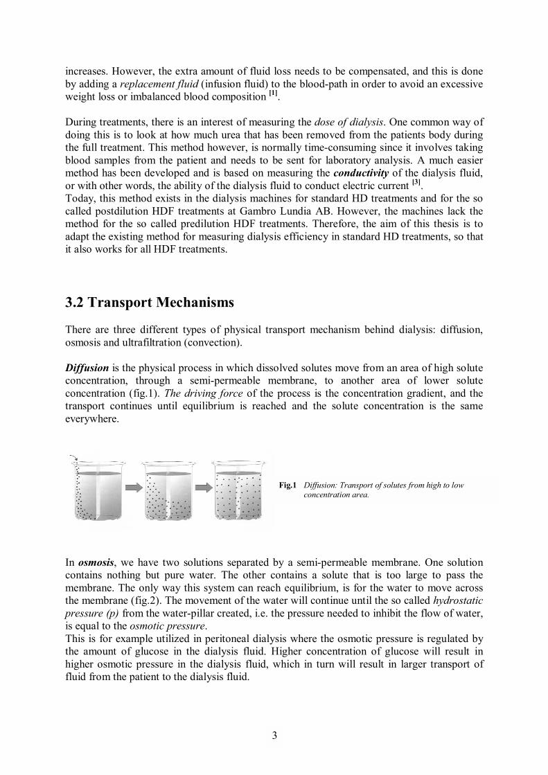
increases. However, the extra amount of fluid loss needs to be compensated, and this is done by adding a replacement fluid (infusion fluid) to the blood-path in order to avoid an excessive weight loss or imbalanced blood composition [1]. During treatments, there is an interest of measuring the dose of dialysis. One common way of doing this is to look at how much urea that has been removed from the patients body during the full treatment. This method however, is normally time-consuming since it involves taking blood samples from the patient and needs to be sent for laboratory analysis. A much easier method has been developed and is based on measuring the conductivity of the dialysis fluid, or with other words, the ability of the dialysis fluid to conduct electric current [3]. Today, this method exists in the dialysis machines for standard HD treatments and for the so called postdilution HDF treatments at Gambro Lundia AB. However, the machines lack the method for the so called predilution HDF treatments. Therefore, the aim of this thesis is to adapt the existing method for measuring dialysis efficiency in standard HD treatments, so that it also works for all HDF treatments. 3.2 Transport Mechanisms There are three different types of physical transport mechanism behind dialysis: diffusion, osmosis and ultrafiltration (convection). Diffusion is the physical process in which dissolved solutes move from an area of high solute concentration, through a semi-permeable membrane, to another area of lower solute concentration (fig.1). The driving force of the process is the concentration gradient, and the transport continues until equilibrium is reached and the solute concentration is the same everywhere.

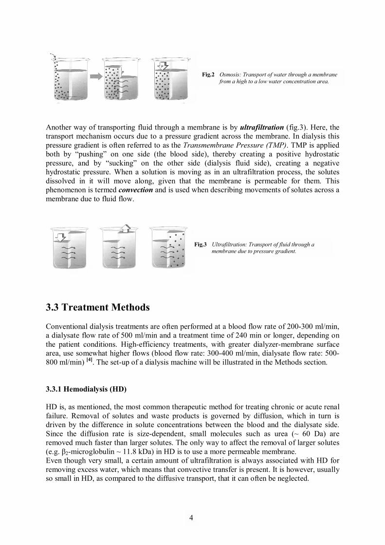
In osmosis, we have two solutions separated by a semi-permeable membrane. One solution contains nothing but pure water. The other contains a solute that is too large to pass the membrane. The only way this system can reach equilibrium, is for the water to move across the membrane (fig.2). The movement of the water will continue until the so called hydrostatic pressure (p) from the water-pillar created, i.e. the pressure needed to inhibit the flow of water, is equal to the osmotic pressure. This is for example utilized in peritoneal dialysis where the osmotic pressure is regulated by the amount of glucose in the dialysis fluid. Higher concentration of glucose will result in higher osmotic pressure in the dialysis fluid, which in turn will result in larger transport of fluid from the patient to the dialysis fluid.

Fig.1 Diffusion: Transport of solutes from high to low concentration area.

3

1

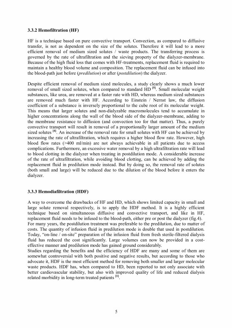
Another way of transporting fluid through a membrane is by ultrafiltration (fig.3). Here, the transport mechanism occurs due to a pressure gradient across the membrane. In dialysis this pressure gradient is often referred to as the Transmembrane Pressure (TMP). TMP is applied both by �pushing� on one side (the blood side), thereby creating a positive hydrostatic pressure, and by �sucking� on the other side (dialysis fluid side), creating a negative hydrostatic pressure. When a solution is moving as in an ultrafiltration process, the solutes dissolved in it will move along, given that the membrane is permeable for them. This phenomenon is termed convection and is used when describing movements of solutes across a membrane due to fluid flow.

3.3 Treatment Methods Conventional dialysis treatments are often performed at a blood flow rate of 200-300 ml/min, a dialysate flow rate of 500 ml/min and a treatment time of 240 min or longer, depending on the patient conditions. High-efficiency treatments, with greater dialyzer-membrane surface area, use somewhat higher flows (blood flow rate: 300-400 ml/min, dialysate flow rate: 500-800 ml/min) [4]. The set-up of a dialysis machine will be illustrated in the Methods section. 3.3.1 Hemodialysis (HD) HD is, as mentioned, the most common therapeutic method for treating chronic or acute renal failure. Removal of solutes and waste products is governed by diffusion, which in turn is driven by the difference in solute concentrations between the blood and the dialysate side. Since the diffusion rate is size-dependent, small molecules such as urea (~ 60 Da) are removed much faster than larger solutes. The only way to affect the removal of larger solutes (e.g. β2-microglobulin ~ 11.8 kDa) in HD is to use a more permeable membrane. Even though very small, a certain amount of ultrafiltration is always associated with HD for removing excess water, which means that convective transfer is present. It is however, usually so small in HD, as compared to the diffusive transport, that it can often be neglected.

Fig.3 Ultrafiltration: Transport of fluid through a membrane due to pressure gradient.

Fig.2 Osmosis: Transport of water through a membrane from a high to a low water concentration area.

4

1

3.3.2 Hemofiltration (HF) HF is a technique based on pure convective transport. Convection, as compared to diffusive transfer, is not as dependent on the size of the solutes. Therefore it will lead to a more efficient removal of medium sized solutes / waste products. The transferring process is governed by the rate of ultrafiltration and the sieving property of the dialyzer-membrane. Because of the high fluid loss that comes with HF-treatments, replacement fluid is required to maintain a healthy blood volume and composition. The replacement fluid can be infused into the blood-path just before (predilution) or after (postdilution) the dialyzer. Despite efficient removal of medium sized molecules, a study clearly shows a much lower removal of small sized solutes, when compared to standard HD [5]. Small molecular weight substances, like urea, are removed at a faster rate with HD, whereas medium sized substances are removed much faster with HF. According to Einstein / Nernst law, the diffusion coefficient of a substance is inversely proportional to the cube root of its molecular weight. This means that larger solutes and non-dialyzable macromolecules tend to accumulate in higher concentrations along the wall of the blood side of the dialyzer-membrane, adding to the membrane resistance to diffusion (and convection too for that matter). Thus, a purely convective transport will result in removal of a proportionally larger amount of the medium sized solutes [4]. An increase of the removal rate for small solutes with HF can be achieved by increasing the rate of ultrafiltration, which requires a higher blood flow rate. However, high blood flow rates (>400 ml/min) are not always achievable in all patients due to access complications. Furthermore, an excessive water removal by a high ultrafiltration rate will lead to blood clotting in the dialyzer when treating in postdilution mode. A considerable increase of the rate of ultrafiltration, while avoiding blood clotting, can be achieved by adding the replacement fluid in predilution mode instead. But by doing so, the removal rate of solutes (both small and large) will be reduced due to the dilution of the blood before it enters the dialyzer. 3.3.3 Hemodiafiltration (HDF) A way to overcome the drawbacks of HF and HD, which shows limited capacity in small and large solute removal respectively, is to apply the HDF method. It is a highly efficient technique based on simultaneous diffusive and convective transport, and like in HF, replacement fluid needs to be infused to the blood-path, either pre or post the dialyzer (fig.4). For many years, the postdilution treatment was preferable to the predilution, due to matter of costs. The quantity of infusion fluid in predilution mode is double that used in postdilution. Today, �on-line / on-site� preparation of the infusion fluid from fresh sterile-filtered dialysis fluid has reduced the cost significantly. Large volumes can now be provided in a cost-effective manner and predilution mode has gained ground considerably. Studies regarding the benefits and the efficiency of HDF are many and some of them are somewhat controversial with both positive and negative results, but according to those who advocate it, HDF is the most efficient method for removing both smaller and larger molecular waste products. HDF has, when compared to HD, been reported to not only associate with better cardiovascular stability, but also with improved quality of life and reduced dialysis related morbidity in long-term treated patients [1].

5

1

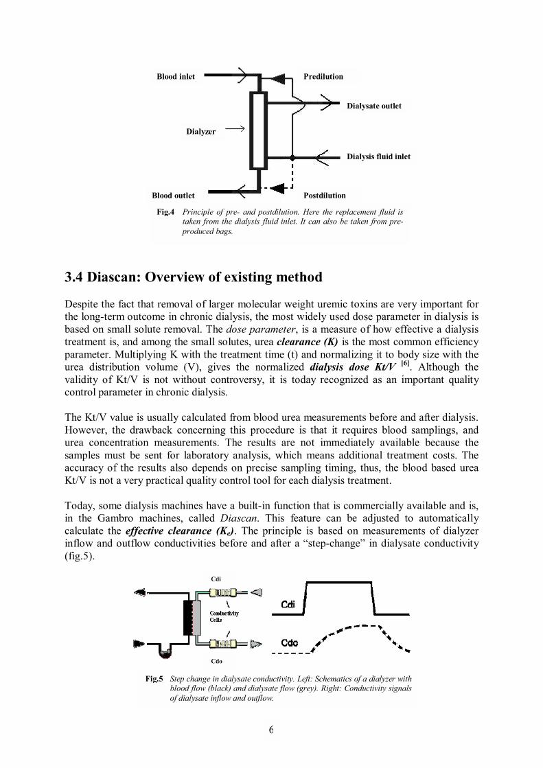
3.4 Diascan: Overview of existing method Despite the fact that removal of larger molecular weight uremic toxins are very important for the long-term outcome in chronic dialysis, the most widely used dose parameter in dialysis is based on small solute removal. The dose parameter, is a measure of how effective a dialysis treatment is, and among the small solutes, urea clearance (K) is the most common efficiency parameter. Multiplying K with the treatment time (t) and normalizing it to body size with the urea distribution volume (V), gives the normalized dialysis dose Kt/V [6]. Although the validity of Kt/V is not without controversy, it is today recognized as an important quality control parameter in chronic dialysis. The Kt/V value is usually calculated from blood urea measurements before and after dialysis. However, the drawback concerning this procedure is that it requires blood samplings, and urea concentration measurements. The results are not immediately available because the samples must be sent for laboratory analysis, which means additional treatment costs. The accuracy of the results also depends on precise sampling timing, thus, the blood based urea Kt/V is not a very practical quality control tool for each dialysis treatment. Today, some dialysis machines have a built-in function that is commercially available and is, in the Gambro machines, called Diascan. This feature can be adjusted to automatically calculate the effective clearance (Ke). The principle is based on measurements of dialyzer inflow and outflow conductivities before and after a �step-change� in dialysate conductivity (fig.5).

Fig.5 Step change in dialysate conductivity. Left: Schematics of a dialyzer withblood flow (black) and dialysate flow (grey). Right: Conductivity signals of dialysate inflow and outflow.

Cdi

Cdo

Dialyzer

Blood inlet

Blood outlet

Dialysis fluid inlet

Dialysate outlet

Predilution

Postdilution

Fig.4 Principle of pre- and postdilution. Here the replacement fluid is taken from the dialysis fluid inlet. It can also be taken from pre-produced bags.

6

1

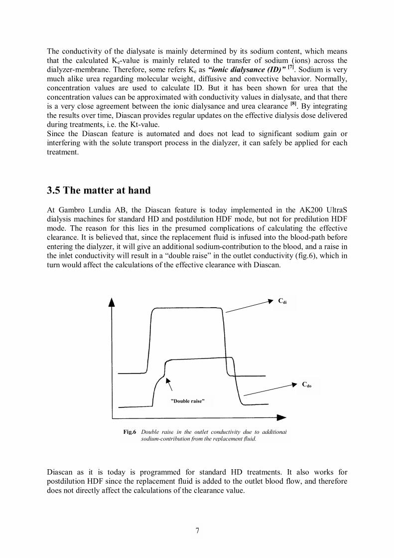
The conductivity of the dialysate is mainly determined by its sodium content, which means that the calculated Ke-value is mainly related to the transfer of sodium (ions) across the dialyzer-membrane. Therefore, some refers Ke as �ionic dialysance (ID)� [7]. Sodium is very much alike urea regarding molecular weight, diffusive and convective behavior. Normally, concentration values are used to calculate ID. But it has been shown for urea that the concentration values can be approximated with conductivity values in dialysate, and that there is a very close agreement between the ionic dialysance and urea clearance [8]. By integrating the results over time, Diascan provides regular updates on the effective dialysis dose delivered during treatments, i.e. the Kt-value. Since the Diascan feature is automated and does not lead to significant sodium gain or interfering with the solute transport process in the dialyzer, it can safely be applied for each treatment. 3.5 The matter at hand At Gambro Lundia AB, the Diascan feature is today implemented in the AK200 UltraS dialysis machines for standard HD and postdilution HDF mode, but not for predilution HDF mode. The reason for this lies in the presumed complications of calculating the effective clearance. It is believed that, since the replacement fluid is infused into the blood-path before entering the dialyzer, it will give an additional sodium-contribution to the blood, and a raise in the inlet conductivity will result in a �double raise� in the outlet conductivity (fig.6), which in turn would affect the calculations of the effective clearance with Diascan.

Diascan as it is today is programmed for standard HD treatments. It also works for postdilution HDF since the replacement fluid is added to the outlet blood flow, and therefore does not directly affect the calculations of the clearance value.

Cdo

Cdi

�Double raise�

Fig.6 Double raise in the outlet conductivity due to additional sodium-contribution from the replacement fluid.

7

1

The main purpose of this thesis is to adapt the Diascan method for calculating the effective clearance, to predilution HDF mode, on an AK200 UltraS dialysis machine. A first step towards the goal is to comprehend the existing method and calculations for standard HD. Measurements on the dialysis machine will then be performed during simulated treatments in the laboratory, and modification of the existing method, will be based on the data from these measurements. As a secondary objective, results from the trials with the modified method will be tested against a theoretical formula for how the efficiency depends on various factors like blood flow, dialysis fluid flow and replacement fluid flow. This part is meant as an evaluation of how good the theoretical formula really is, which today is rather debated.

8

1

4 Theory Here follows a detailed account of the calculations used in this project starting with a general description of the term �clearance�, and ending with derived formula specific for the method previously described. 4.1 The Concept of Clearance / Dialysance In order to describe the cleansing capacity of a dialyzer, the term Clearance (K) is introduced. Clearance is defined as the theoretical amount of blood that has been totally cleared of a given solute in a given amount of time and can mathematically be expressed as:

[mmol/ml] tion)(Concentra C force, Driving[mmol/min] J rate, Removal[ml/min]K Clearance, = [4] (1)

Depending on whether the blood side or the dialysis fluid side is being considered, the removal rate (J) across the dialyzer can be expressed as:

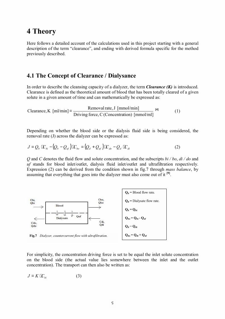
( ) ( ) diddoufdboufbbib CQCQQCQQCQJ ⋅−⋅+=⋅−−⋅= (2) Q and C denotes the fluid flow and solute concentration, and the subscripts bi / bo, di / do and uf stands for blood inlet/outlet, dialysis fluid inlet/outlet and ultrafiltration respectively. Expression (2) can be derived from the condition shown in fig.7 through mass balance, by assuming that everything that goes into the dialyzer must also come out of it [9].

For simplicity, the concentration driving force is set to be equal the inlet solute concentration on the blood side (the actual value lies somewhere between the inlet and the outlet concentration). The transport can then also be written as:

biCKJ ⋅= (3)

Fig.7 Dialyzer, countercurrent flow with ultrafiltration.

Qb = Blood flow rate.

Qd = Dialysate flow rate.

Qb = Qbi

Qbo = Qbi - Quf

Qd = Qdi

Qdo = Qdi + Quf

9

1

When talking about clearance, the solute considered is not present in the dialysis fluid, as in the case of urea. When the solute also is present in the dialysis fluid, like e.g. Na+, clearance is instead referred to as Dialysance (D). The concentration driving force is then equal to the difference between the inlet solute concentration on the blood side and dialysis fluid side, and the following yields for the transport:

( )dibi CCDJ −⋅= [9] (4) The removal rate described in this way however, was shown by Ross et al. [10] to only be useful in the special case where we merely have diffusive substances, that is Quf = 0. According to Ross, the actual removal rate (J) is a combination of diffusive and convective transport and in presence of ultrafiltration, J is not proportional to (Cbi � Cdi) but rather, it is a linear function of Cbi and Cdi:

didbib CKCKJ ⋅−⋅= (5) by which the coefficients Kb and Kd, independent of the concentrations, are referred to as the �generalized clearances�. Ross also talks about a transmittance factor (0 ≤ TR ≤ 1), which describes the fraction of the solute dragged through the membrane by ultrafiltration. In the case where TR = 1, i.e. when no reflection of the solute occurs, the following relationship is true for the generalized clearances:

ufdb QKK =− (6) Combining equation (5) with equation (6) and rearranging, allows the transport to be written as:

diufdibib CQCCKJ ⋅+−⋅= )( (7) By writing equation (7) in this way, the removal rate can be quantified as a function of the solute concentrations Cbi, Cdi and the generalized clearance Kb, which take into account the influence of convective transport (ultrafiltration). From the definition stated above, D can be written as:

( ) dibi

diufb

dibi CCCQ

KCC

JD−⋅

+=−

= (8)

As can be seen, D is dependent of the solute concentration around the dialyzer, which is constantly changing during a treatment, and is therefore not a constant value.

10

1

4.2 The Diascan Formula Combining equation (2) and (7) yields for the dialysate side:

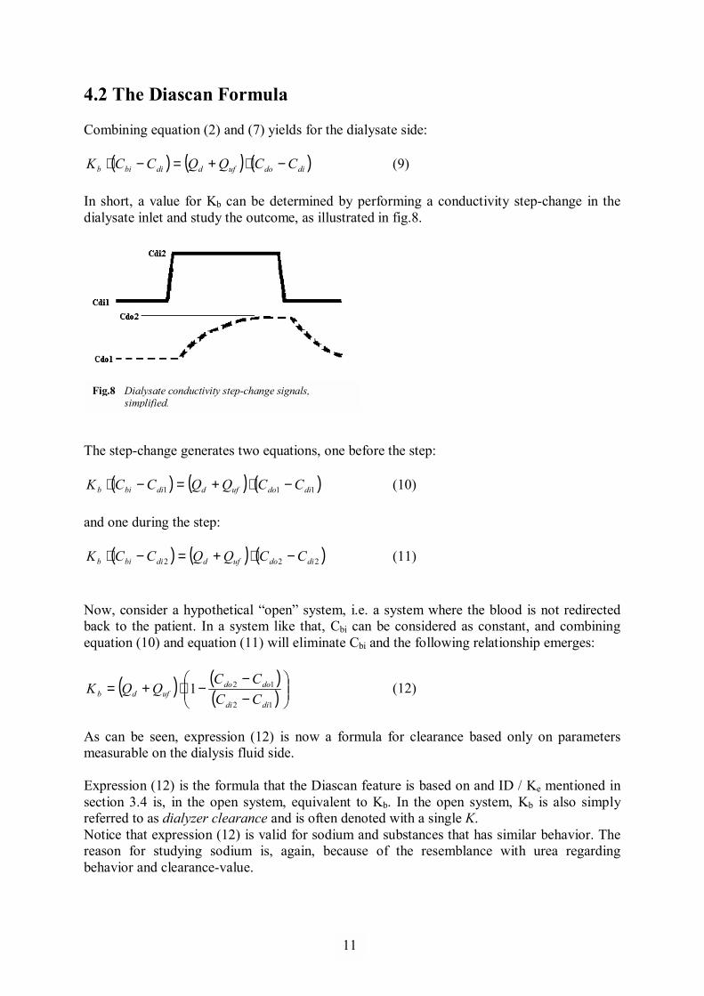
( ) ( ) ( )didoufddibib CCQQCCK −⋅+=−⋅ (9) In short, a value for Kb can be determined by performing a conductivity step-change in the dialysate inlet and study the outcome, as illustrated in fig.8.

The step-change generates two equations, one before the step:

( ) ( ) ( )111 didoufddibib CCQQCCK −⋅+=−⋅ (10) and one during the step:

( ) ( ) ( )222 didoufddibib CCQQCCK −⋅+=−⋅ (11) Now, consider a hypothetical �open� system, i.e. a system where the blood is not redirected back to the patient. In a system like that, Cbi can be considered as constant, and combining equation (10) and equation (11) will eliminate Cbi and the following relationship emerges:

( ) ( )( )

−−

−⋅+=12

121didi

dodoufdb CC

CCQQK (12)

As can be seen, expression (12) is now a formula for clearance based only on parameters measurable on the dialysis fluid side. Expression (12) is the formula that the Diascan feature is based on and ID / Ke mentioned in section 3.4 is, in the open system, equivalent to Kb. In the open system, Kb is also simply referred to as dialyzer clearance and is often denoted with a single K. Notice that expression (12) is valid for sodium and substances that has similar behavior. The reason for studying sodium is, again, because of the resemblance with urea regarding behavior and clearance-value.

Fig.8 Dialysate conductivity step-change signals, simplified.

11

1

4.3 From Concentration to Conductivity There is a strong relation between the concentration and the conductivity of ions. The total conductivity, κtot, in a solution is given by the conductivity contributions of each and every component, κi, in the solution [4]:

∑=

=N

iitot

1κκ (13)

N is the total number of components in the system. The contribution of a single component, κi, is given by:

iii CI ⋅Λ= )(κ (14) Λi(I) is the so called molar conductivity of the component i at the ionic strength I. Ci is the concentration of the component i in the solution. Further, the ionic strength basically tells how strong the forces between the ions in a solution are, and is given by:

∑=

⋅⋅=n

iii ZCI

1

2

21 (15)

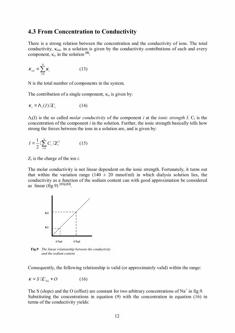
Zi is the charge of the ion i. The molar conductivity is not linear dependent on the ionic strength. Fortunately, it turns out that within the variation range (140 ± 20 mmol/ml) in which dialysis solution lies, the conductivity as a function of the sodium content can with good approximation be considered as linear (fig.9) [11],[12]. Consequently, the following relationship is valid (or approximately valid) within the range:

OCS Na +⋅=κ (16) The S (slope) and the O (offset) are constant for two arbitrary concentrations of Na+ in fig.9. Substituting the concentrations in equation (9) with the concentration in equation (16) in terms of the conductivity yields:

Κ2

Κ1

CNa1 CNa2

Fig.9 The linear relationship between the conductivity and the sodium content.

12

1

( )

−−

−⋅+=

−−

−⋅

di

didi

do

dodoufd

di

didi

bi

bibib S

OS

OQQ

SO

SO

Kκκκκ

(17)

As said, in solutions where only CNa+ is varied, equation (16) is valid. Different solutions have different S and O, but the dialysis fluid before the dialyzer can be considered as one solution (before and during the step-change) and after the dialyzer as another solution. For these �solutions�, O is different but S is approximately the same, so (17) reduces to:

( ) ( )[ ] ( ) ( ) ( )[ ]dididodoufddidibibib OOQQOOK −−−⋅+=−−−⋅ κκκκ (18) Performing a step-change and rearranging as in previous section yields:

( ) ( ) ( )[ ]( ) ( )[ ]

−−−−−−

−⋅+=idiidi

odoodoufdb OO

OOQQK

12

121κκκκ

(19)

which ultimately gives:

( ) ( )( )

−−

−⋅+=12

121didi

dodoufdb QQK

κκκκ

(20)

Thus, the sodium concentration values can be accurately substituted by conductivity values. 4.4 The Donnan-factor Regarding blood, it is important to mention that when dealing with semi-permeable membranes and proteins, the Gibbs-Donnan effect has to be taken into account. The Gibbs-Donnan effect occurs when large particles like proteins in the blood cannot pass the membrane and thereby give rise to osmosis. These proteins are also often negatively charged and attract or bind positively charged ions (such as Na+) which thereby fail to distribute evenly across the membrane. When performing calculations, the concentration on the blood side must be adjusted with the Donnan-factor (α), defined as the ratio of ionic concentrations in dialysate and blood at equilibrium [13]. For positively charged ions, α lies between 0 and 1, and for negatively charged ions, α is greater than 1. 4.5 The Theoretical Formula There have been many attempts to theoretically describe what effects ultrafiltration has on clearance. The theories used so far, are actually based on a more practical approach, using one-dimensional theory that neglects the concentration profiles inside blood and dialysate channels and describes only average concentrations [15]. Calculating the ultrafiltration effects is quite complicated, and by simply adding the ultrafiltration rate to the diffusive clearance will in most times overestimate the total

13

1

clearance. It is because such an addition would assume that the ultrafiltrate drawn from the blood has the same solute concentration as the inlet blood concentration. The real ultrafiltrate solute concentration actually represents the average blood concentration over the length of the dialyzer. Another effect of ultrafiltration is that it changes the flow rates, and thereby also the concentration profile along the dialyzer, which affects the total diffusion. One theoretical expression that deals with these factors is given by:

( ) ( )( )ufbd

ufdufbdb

QQfQQQQQfQQ

K−⋅−

+⋅−⋅−⋅= [16] (21)

where f is further given by:

γ/1

+⋅

−=

d

ufd

b

ufb

QQQ

QQQ

f with 1/ −= kAQufeγ , (22)

Qb, Qd and Quf denote the inlet blood flow rate, inlet dialysate flow rate and ultrafiltration flow rate as before, and kA is the diffusive solute permeability of the dialyzer.

14

1

5 Method �The main purpose of this study is to adapt the Diascan method for calculating the effective clearance, in predilution HDF mode, on an AK200 UltraS dialysis machine� 5.1 Equipment

• AK200 UltraS (Dialysis machine; Gambro). • BL200B Pre/Post (Blood tubing set; Gambro). • Polyflux 170H (Capillary Dialyzer / - Filter; Gambro). • UltraSteriSet (Infusate tubing set with U 2000 ultra filter; Gambro). • D01 Acetate (Haemodialysis Concentrate; Gambro). • Container 20L (Container storing dialysis fluid and representing the human body). • Desktop: PC, OS Microsoft Windows XP. • Software: GLS v2.06 (Logging program, Gambro), LogTool v2.51 BETA (Extraction

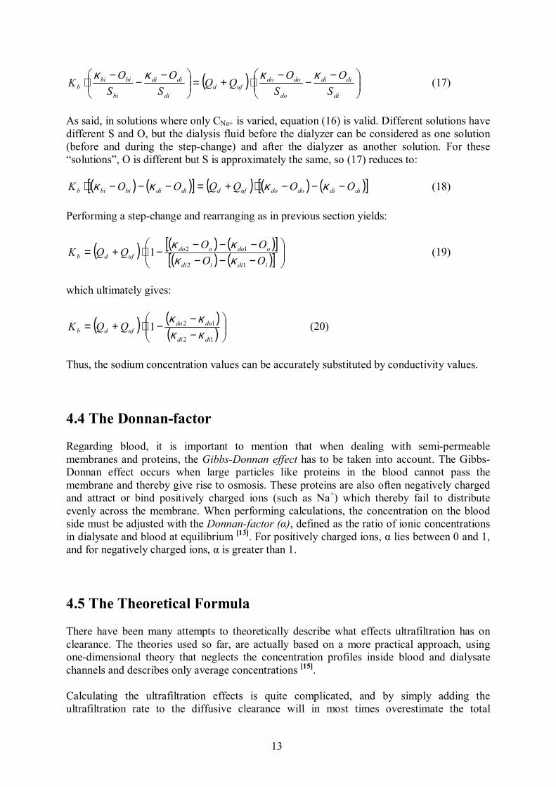
tool, Gambro), Mathworks Matlab v7.0.1, 5.2 Experimental Set-up The pictures below (fig.10-12) illustrate the experimental set-up of the AK200 UltraS dialysis machine used in this study:

Fig.10 The AK200 UltraS dialysis machine.

Control panel. �Patient� status and flow rates are monitored and adjusted here.

Blood pump with the arterial blood tube.

20L Container, containing dialysis fluid which represents the human body.

Infusion pump with infusion tube. Delivers the replacement fluid when running in HDF mode.

Polyflux 170H Dialyzer. Here is where the transport of solutes and waste products from the blood to dialysis fluid occur.

D01 Acetate, Dialysis concentrate.

15

1

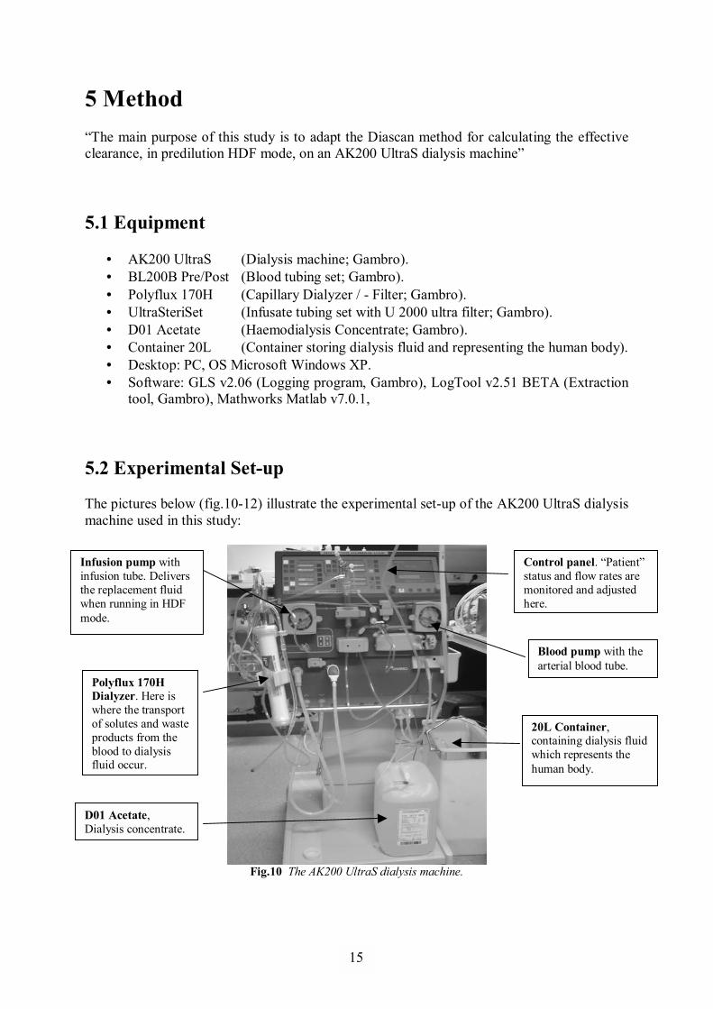
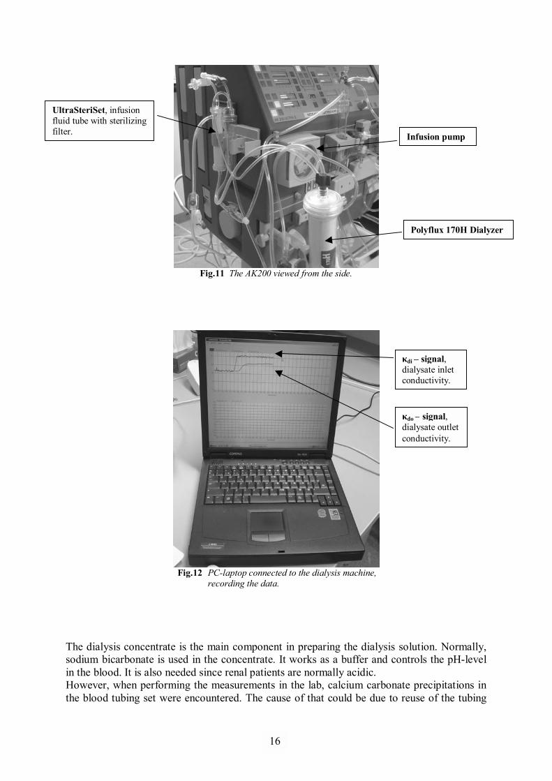
Fig.11 The AK200 viewed from the side.

Fig.12 PC-laptop connected to the dialysis machine, recording the data. The dialysis concentrate is the main component in preparing the dialysis solution. Normally, sodium bicarbonate is used in the concentrate. It works as a buffer and controls the pH-level in the blood. It is also needed since renal patients are normally acidic. However, when performing the measurements in the lab, calcium carbonate precipitations in the blood tubing set were encountered. The cause of that could be due to reuse of the tubing

Infusion pump

Polyflux 170H Dialyzer

UltraSteriSet, infusion fluid tube with sterilizing filter.

κdo � signal, dialysate outlet conductivity.

κdi � signal, dialysate inlet conductivity.

16

1

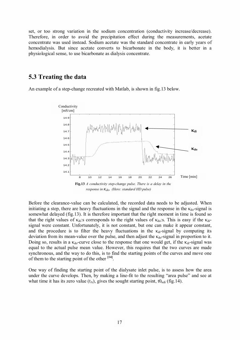
set, or too strong variation in the sodium concentration (conductivity increase/decrease). Therefore, in order to avoid the precipitation effect during the measurements, acetate concentrate was used instead. Sodium acetate was the standard concentrate in early years of hemodialysis. But since acetate converts to bicarbonate in the body, it is better in a physiological sense, to use bicarbonate as dialysis concentrate. 5.3 Treating the data An example of a step-change recreated with Matlab, is shown in fig.13 below.

8 10 12 14 16 18 20 22 24 26

14.1

14.2

14.3

14.4

14.5

14.6

14.7

14.8

14.9

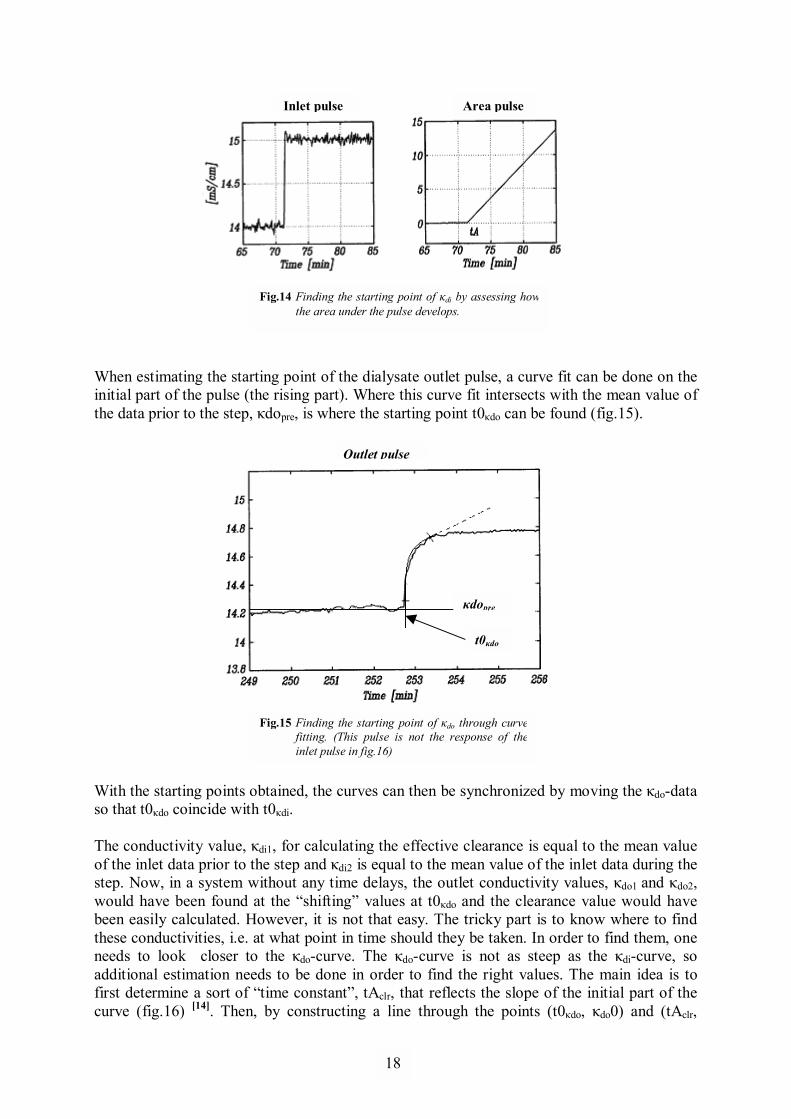
Before the clearance-value can be calculated, the recorded data needs to be adjusted. When initiating a step, there are heavy fluctuations in the signal and the response in the κdo-signal is somewhat delayed (fig.13). It is therefore important that the right moment in time is found so that the right values of κdi:s corresponds to the right values of κdo:s. This is easy if the κdi-signal were constant. Unfortunately, it is not constant, but one can make it appear constant, and the procedure is to filter the heavy fluctuations in the κdi-signal by computing its deviation from its mean-value over the pulse, and then adjust the κdo-signal in proportion to it. Doing so, results in a κdo-curve close to the response that one would get, if the κdi-signal was equal to the actual pulse mean value. However, this requires that the two curves are made synchronous, and the way to do this, is to find the starting points of the curves and move one of them to the starting point of the other [14]. One way of finding the starting point of the dialysate inlet pulse, is to assess how the area under the curve develops. Then, by making a line-fit to the resulting �area pulse� and see at what time it has its zero value (tA), gives the sought starting point, t0κdi (fig.14).

Conductivity [mS/cm]

Time [min]

Fig.13 A conductivity step-change pulse. There is a delay in the response in κdo. (Here: standard HD pulse)

κdo

κdi

17

1

Inlet pulse

Outlet pulse

When estimating the starting point of the dialysate outlet pulse, a curve fit can be done on the initial part of the pulse (the rising part). Where this curve fit intersects with the mean value of the data prior to the step, κdopre, is where the starting point t0κdo can be found (fig.15).

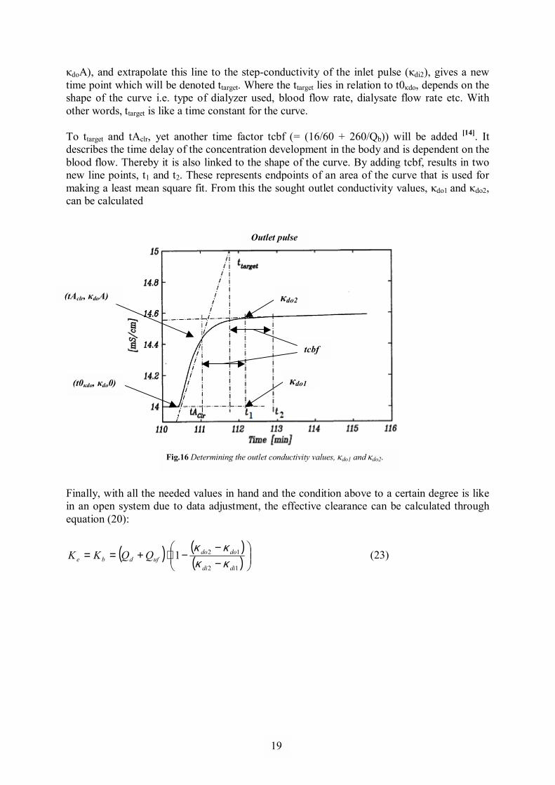
With the starting points obtained, the curves can then be synchronized by moving the κdo-data so that t0κdo coincide with t0κdi. The conductivity value, κdi1, for calculating the effective clearance is equal to the mean value of the inlet data prior to the step and κdi2 is equal to the mean value of the inlet data during the step. Now, in a system without any time delays, the outlet conductivity values, κdo1 and κdo2, would have been found at the �shifting� values at t0κdo and the clearance value would have been easily calculated. However, it is not that easy. The tricky part is to know where to find these conductivities, i.e. at what point in time should they be taken. In order to find them, one needs to look closer to the κdo-curve. The κdo-curve is not as steep as the κdi-curve, so additional estimation needs to be done in order to find the right values. The main idea is to first determine a sort of �time constant�, tAclr, that reflects the slope of the initial part of the curve (fig.16) [14]. Then, by constructing a line through the points (t0κdo, κdo0) and (tAclr,

Area pulse

Fig.14 Finding the starting point of κdi by assessing howthe area under the pulse develops.

t0κdo

κdopre

Fig.15 Finding the starting point of κdo through curve fitting. (This pulse is not the response of theinlet pulse in fig.16)

18

1

κdoA), and extrapolate this line to the step-conductivity of the inlet pulse (κdi2), gives a new time point which will be denoted ttarget. Where the ttarget lies in relation to t0κdo, depends on the shape of the curve i.e. type of dialyzer used, blood flow rate, dialysate flow rate etc. With other words, ttarget is like a time constant for the curve. To ttarget and tAclr, yet another time factor tcbf (= (16/60 + 260/Qb)) will be added [14]. It describes the time delay of the concentration development in the body and is dependent on the blood flow. Thereby it is also linked to the shape of the curve. By adding tcbf, results in two new line points, t1 and t2. These represents endpoints of an area of the curve that is used for making a least mean square fit. From this the sought outlet conductivity values, κdo1 and κdo2, can be calculated

Finally, with all the needed values in hand and the condition above to a certain degree is like in an open system due to data adjustment, the effective clearance can be calculated through equation (20):

( ) ( )( )

−−

−⋅+==12

121didi

dodoufdbe QQKK

κκκκ

(23)

(t0κdo, κdo0)

Outlet pulse

Fig.16 Determining the outlet conductivity values, κdo1 and κdo2.

κdo2

κdo1

tcbf

(tAclr, κdoA)

19

1

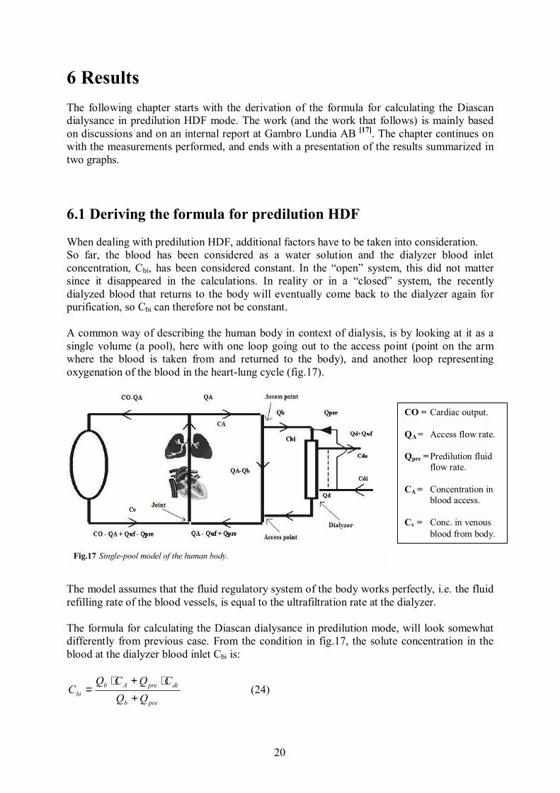
6 Results The following chapter starts with the derivation of the formula for calculating the Diascan dialysance in predilution HDF mode. The work (and the work that follows) is mainly based on discussions and on an internal report at Gambro Lundia AB [17]. The chapter continues on with the measurements performed, and ends with a presentation of the results summarized in two graphs. 6.1 Deriving the formula for predilution HDF When dealing with predilution HDF, additional factors have to be taken into consideration. So far, the blood has been considered as a water solution and the dialyzer blood inlet concentration, Cbi, has been considered constant. In the �open� system, this did not matter since it disappeared in the calculations. In reality or in a �closed� system, the recently dialyzed blood that returns to the body will eventually come back to the dialyzer again for purification, so Cbi can therefore not be constant. A common way of describing the human body in context of dialysis, is by looking at it as a single volume (a pool), here with one loop going out to the access point (point on the arm where the blood is taken from and returned to the body), and another loop representing oxygenation of the blood in the heart-lung cycle (fig.17).

The model assumes that the fluid regulatory system of the body works perfectly, i.e. the fluid refilling rate of the blood vessels, is equal to the ultrafiltration rate at the dialyzer. The formula for calculating the Diascan dialysance in predilution mode, will look somewhat differently from previous case. From the condition in fig.17, the solute concentration in the blood at the dialyzer blood inlet Cbi is:

preb

dipreAbbi QQ

CQCQC

+⋅+⋅

= (24)

Fig.17 Single-pool model of the human body.

CO = Cardiac output.

QA = Access flow rate.

Qpre = Predilution fluid flow rate.

CA = Concentration in blood access.

Cv = Conc. in venous blood from body.

20

1

Again, deriving the transport out of the body yields:

( ) ( ) diddoufddiufdibib CQCQQCQCCK ⋅−⋅+=⋅+−⋅⋅ α ( ) ( ) diufdidoufd CQCCQQ ⋅+−⋅+= (25) Here, Qd is the remaining dialysis fluid rate after the replacement fluid rate has been subtracted, and the Donnan-factor α refers to the blood entering the dialyzer (compare with equation 9). Next, is a mass balance at the joint, where the blood from the body with concentration Cv is mixed with the blood returning from the access point. The mass in the returning blood is the difference between the mass going to the access from the heart and the mass removed in the dialyzer. Given that the ultrafiltration rate, Quf, is the sum of the patient weight loss rate (WL) during treatments and the replacement fluid flow rate Qpre, the mass balance at the joint results in:

( ) ( ) diufdibibAAufAvA CQCCKCQQQCOCCOC ⋅−−⋅⋅−⋅++−⋅=⋅ α (26) Solving equation (26) for CA, inserting it in equation (24), and then solving the resulting expression for Cbi and inserting it in equation (25), gives an expression for (Cdo-Cdi):

( ) ( ) +

−

+⋅

⋅⋅=−⋅+ 1preb

predibdidoufd QQ

QCKCCQQ

α

( )

−

+⋅⋅

−⋅++−⋅⋅

+⋅⋅+−

+⋅⋅

+ ufpreb

prebbdiufAv

preb

bbA

preb

bb

QQQQK

KCQQCOC

QQQ

KQCO

QQQ

Kα

α

α (27)

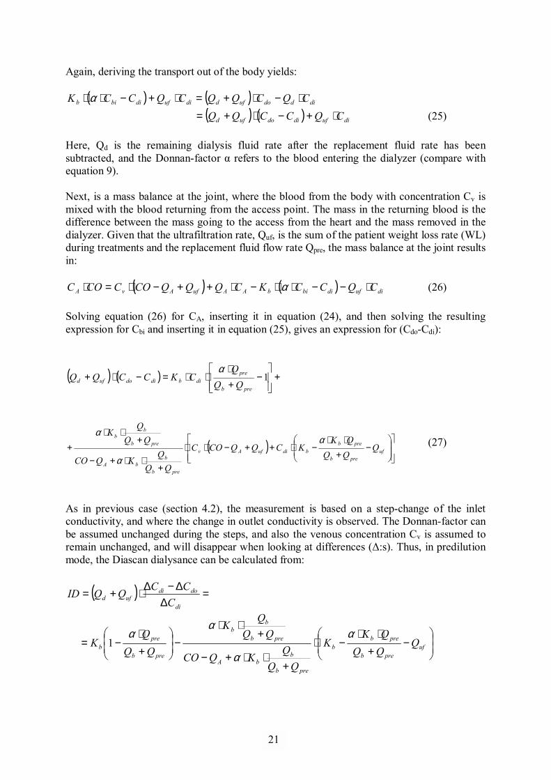
As in previous case (section 4.2), the measurement is based on a step-change of the inlet conductivity, and where the change in outlet conductivity is observed. The Donnan-factor can be assumed unchanged during the steps, and also the venous concentration Cv is assumed to remain unchanged, and will disappear when looking at differences (∆:s). Thus, in predilution mode, the Diascan dialysance can be calculated from:

( ) =∆

∆−∆⋅+=

di

dodiufd C

CCQQID

−

+⋅⋅

−⋅

+⋅⋅+−

+⋅⋅

−

+⋅

−= ufpreb

prebb

preb

bbA

preb

bb

preb

preb Q

QQQK

K

QQQ

KQCO

QQQ

K

QQQ

Kα

α

αα

1

21

1

preb

bbA

ufpreb

prebb

preb

bb

preb

pre

preb

bbAb

QQQ

KQCO

QQQQK

KQQ

QK

QQQ

QQQ

KQCOK

+⋅⋅+−

−

+⋅⋅

−⋅+

⋅⋅−

+⋅

−⋅

+⋅⋅+−⋅

=α

αα

αα 1

[ ]

preb

bbA

ufpreb

bb

preb

preAb

QQQ

KQCO

QQQ

QK

QQQ

QCOK

+⋅⋅+−

⋅+

⋅⋅+

+⋅

−⋅−⋅

=α

αα

1

[ ] ( )

preb

bbA

ufb

preA

preb

bb

QQQ

KQCO

QQ

QQCO

QQQ

K

+⋅⋅+−

⋅+

⋅−+⋅−

⋅+

⋅=α

αα1

1

( )

Apreb

bb

A

uf

b

pre

preb

bb

QCOQQQ

K

QCOQ

QQ

QQQ

KID

−⋅

+⋅⋅+

−⋅

+⋅−

+⋅

+⋅=⇒

11

11

α

αα

(28)

In predilution mode the dilution-factor

+ preb

b

QQQ

clearly has a great impact on the

calculations. In absence of replacement fluid, i.e. when Qpre=0, the treatment is back in standard HD mode and the Diascan feature measures the effective dialyzer clearance Ke, which in this case is Kb corrected for various factors:

A

b

A

uf

b

QCOKQCO

Q

KID

−⋅

+

−⋅

+⋅= α

α

1

1 (29)

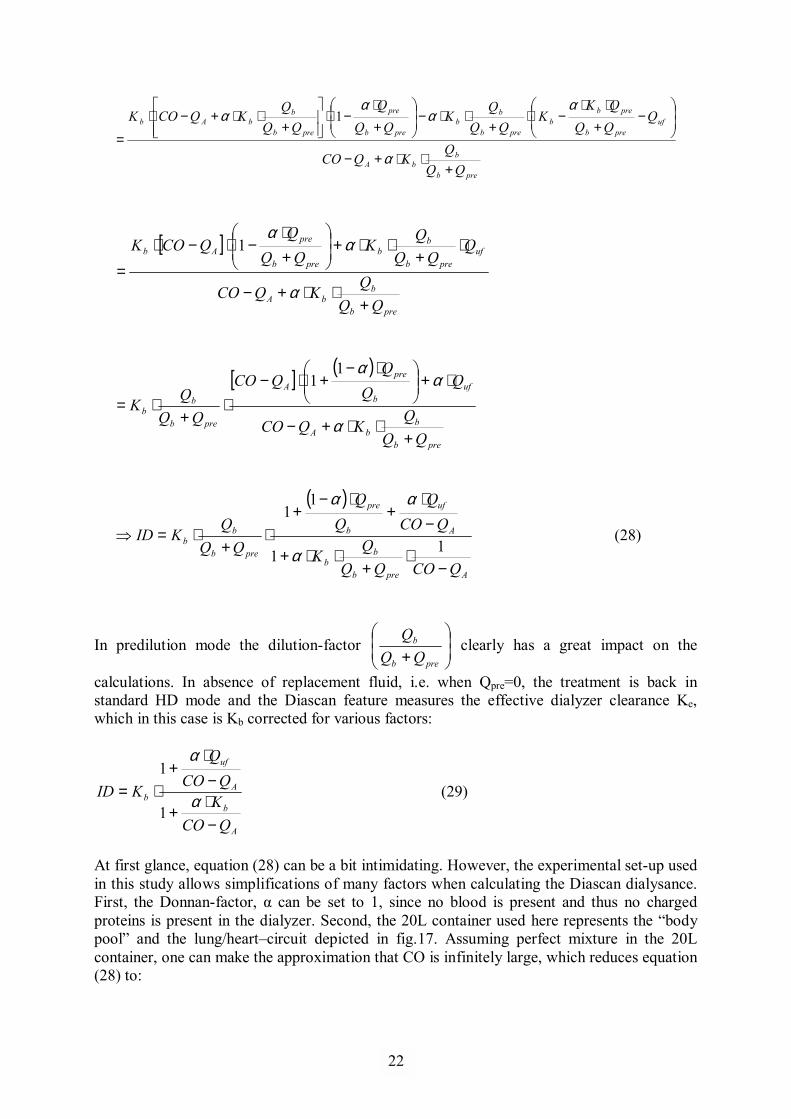
At first glance, equation (28) can be a bit intimidating. However, the experimental set-up used in this study allows simplifications of many factors when calculating the Diascan dialysance. First, the Donnan-factor, α can be set to 1, since no blood is present and thus no charged proteins is present in the dialyzer. Second, the 20L container used here represents the �body pool� and the lung/heart�circuit depicted in fig.17. Assuming perfect mixture in the 20L container, one can make the approximation that CO is infinitely large, which reduces equation (28) to:

22

1

preb

bb QQ

QKID

+⋅= (30)

which is simply equal to the dialyzer clearance, Kb, corrected with the dilution factor

preb

b

QQQ+

.

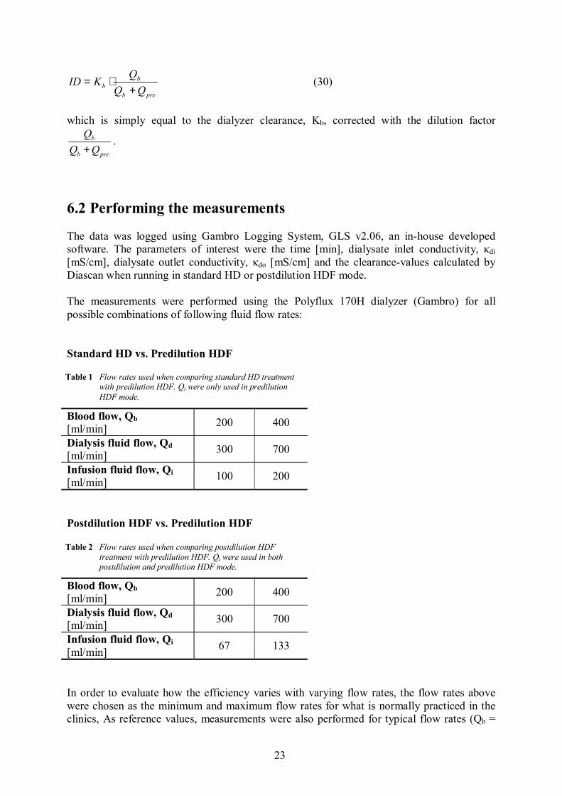
6.2 Performing the measurements The data was logged using Gambro Logging System, GLS v2.06, an in-house developed software. The parameters of interest were the time [min], dialysate inlet conductivity, κdi [mS/cm], dialysate outlet conductivity, κdo [mS/cm] and the clearance-values calculated by Diascan when running in standard HD or postdilution HDF mode. The measurements were performed using the Polyflux 170H dialyzer (Gambro) for all possible combinations of following fluid flow rates: Standard HD vs. Predilution HDF

Blood flow, Qb [ml/min] 200 400

Dialysis fluid flow, Qd [ml/min] 300 700

Infusion fluid flow, Qi [ml/min] 100 200

Postdilution HDF vs. Predilution HDF

Blood flow, Qb [ml/min] 200 400

Dialysis fluid flow, Qd [ml/min] 300 700

Infusion fluid flow, Qi [ml/min] 67 133

In order to evaluate how the efficiency varies with varying flow rates, the flow rates above were chosen as the minimum and maximum flow rates for what is normally practiced in the clinics, As reference values, measurements were also performed for typical flow rates (Qb =

Table 1 Flow rates used when comparing standard HD treatment with predilution HDF. Qi were only used in predilution HDF mode.

Table 2 Flow rates used when comparing postdilution HDF treatment with predilution HDF. Qi were used in both postdilution and predilution HDF mode.

23

1

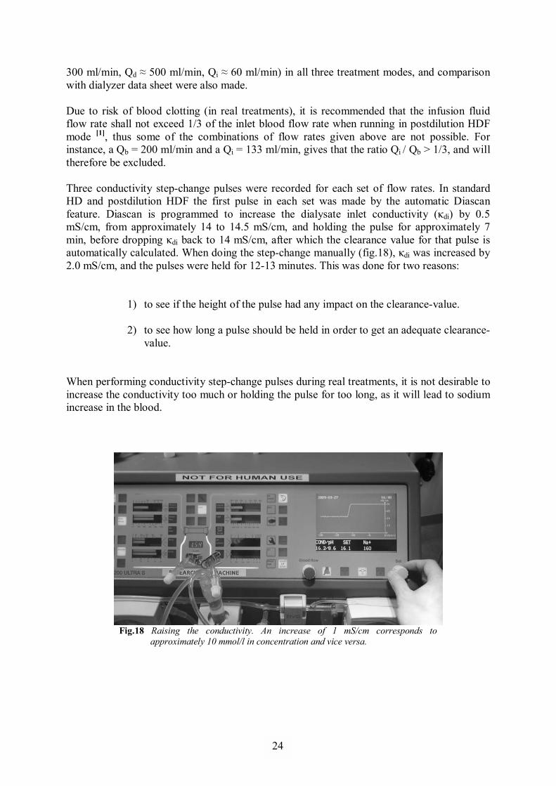
300 ml/min, Qd ≈ 500 ml/min, Qi ≈ 60 ml/min) in all three treatment modes, and comparison with dialyzer data sheet were also made. Due to risk of blood clotting (in real treatments), it is recommended that the infusion fluid flow rate shall not exceed 1/3 of the inlet blood flow rate when running in postdilution HDF mode [1], thus some of the combinations of flow rates given above are not possible. For instance, a Qb = 200 ml/min and a Qi = 133 ml/min, gives that the ratio Qi / Qb > 1/3, and will therefore be excluded. Three conductivity step-change pulses were recorded for each set of flow rates. In standard HD and postdilution HDF the first pulse in each set was made by the automatic Diascan feature. Diascan is programmed to increase the dialysate inlet conductivity (κdi) by 0.5 mS/cm, from approximately 14 to 14.5 mS/cm, and holding the pulse for approximately 7 min, before dropping κdi back to 14 mS/cm, after which the clearance value for that pulse is automatically calculated. When doing the step-change manually (fig.18), κdi was increased by 2.0 mS/cm, and the pulses were held for 12-13 minutes. This was done for two reasons:

1) to see if the height of the pulse had any impact on the clearance-value.

2) to see how long a pulse should be held in order to get an adequate clearance-value.

When performing conductivity step-change pulses during real treatments, it is not desirable to increase the conductivity too much or holding the pulse for too long, as it will lead to sodium increase in the blood.

Fig.18 Raising the conductivity. An increase of 1 mS/cm corresponds to

approximately 10 mmol/l in concentration and vice versa.

24

1

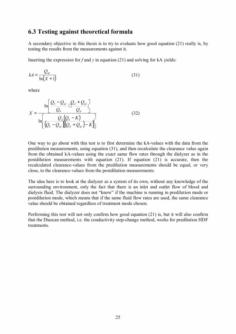
6.3 Testing against theoretical formula A secondary objective in this thesis is to try to evaluate how good equation (21) really is, by testing the results from the measurements against it. Inserting the expression for f and γ in equation (21) and solving for kA yields:

( )1ln +=

XQ

kA uf (31)

where

( )( ) ( )[ ]

−+−−

+⋅

−

=

KQQQQKQQ

QQQ

QQQ

X

ufdufb

bd

d

ufd

b

ufb

ln

ln (32)

One way to go about with this test is to first determine the kA-values with the data from the predilution measurements, using equation (31), and then recalculate the clearance value again from the obtained kA-values using the exact same flow rates through the dialyzer as in the postdilution measurements with equation (21). If equation (21) is accurate, then the recalculated clearance-values from the predilution measurements should be equal, or very close, to the clearance-values from the postdilution measurements. The idea here is to look at the dialyzer as a system of its own, without any knowledge of the surrounding environment, only the fact that there is an inlet and outlet flow of blood and dialysis fluid. The dialyzer does not �know� if the machine is running in predilution mode or postdilution mode, which means that if the same fluid flow rates are used, the same clearance value should be obtained regardless of treatment mode chosen. Performing this test will not only confirm how good equation (21) is, but it will also confirm that the Diascan method, i.e. the conductivity step-change method, works for predilution HDF treatments.

25

1

6.4 Results: Standard HD vs. Predilution HDF

Standard HD vs. Predilution HDF

0

50

100

150

200

250

300

350

400

450

500

0 1 2 3 4 5 6

Measurement set

Clea

ranc

e [m

l/min

]

Pre-HDF (Qi=200 ml/min)Pre-HDF (Qi=100 ml/min)Standard HD

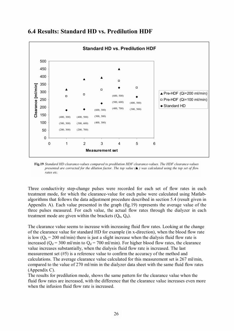
Three conductivity step-change pulses were recorded for each set of flow rates in each treatment mode, for which the clearance-value for each pulse were calculated using Matlab-algorithms that follows the data adjustment procedure described in section 5.4 (result given in Appendix A). Each value presented in the graph (fig.19) represents the average value of the three pulses measured. For each value, the actual flow rates through the dialyzer in each treatment mode are given within the brackets (Qb, Qd). The clearance value seems to increase with increasing fluid flow rates. Looking at the change of the clearance value for standard HD for example (in x-direction), when the blood flow rate is low (Qb = 200 ml/min) there is just a slight increase when the dialysis fluid flow rate is increased (Qd = 300 ml/min to Qd = 700 ml/min). For higher blood flow rates, the clearance value increases substantially, when the dialysis fluid flow rate is increased. The last measurement set (#5) is a reference value to confirm the accuracy of the method and calculations. The average clearance value calculated for this measurement set is 267 ml/min, compared to the value of 270 ml/min in the dialyzer data sheet with the same fluid flow rates (Appendix C). The results for predilution mode, shows the same pattern for the clearance value when the fluid flow rates are increased, with the difference that the clearance value increases even more when the infusion fluid flow rate is increased.

Fig.19 Standard HD clearance-values compared to predilution HDF clearance-values. The HDF clearance-values presented are corrected for the dilution factor. The top value (▲) was calculated using the top set of flow rates etc.

(400, 300) (300, 300) (200, 300)

(400, 500) (300, 600) (200, 700)

(600, 300) (500, 300) (400, 300)

(600, 500) (500, 600) (400, 700)

(400, 500) (300, 500)

26

1

6.5 Results: Postdilution HDF vs. Predilution HDF

Postdilution HDF vs. Predilution HDF

0

50

100

150

200

250

300

350

400

0 2 4 6 8

Measurement set

Clea

ranc

e [m

l/min

]

Pre-HDFPost-HDF

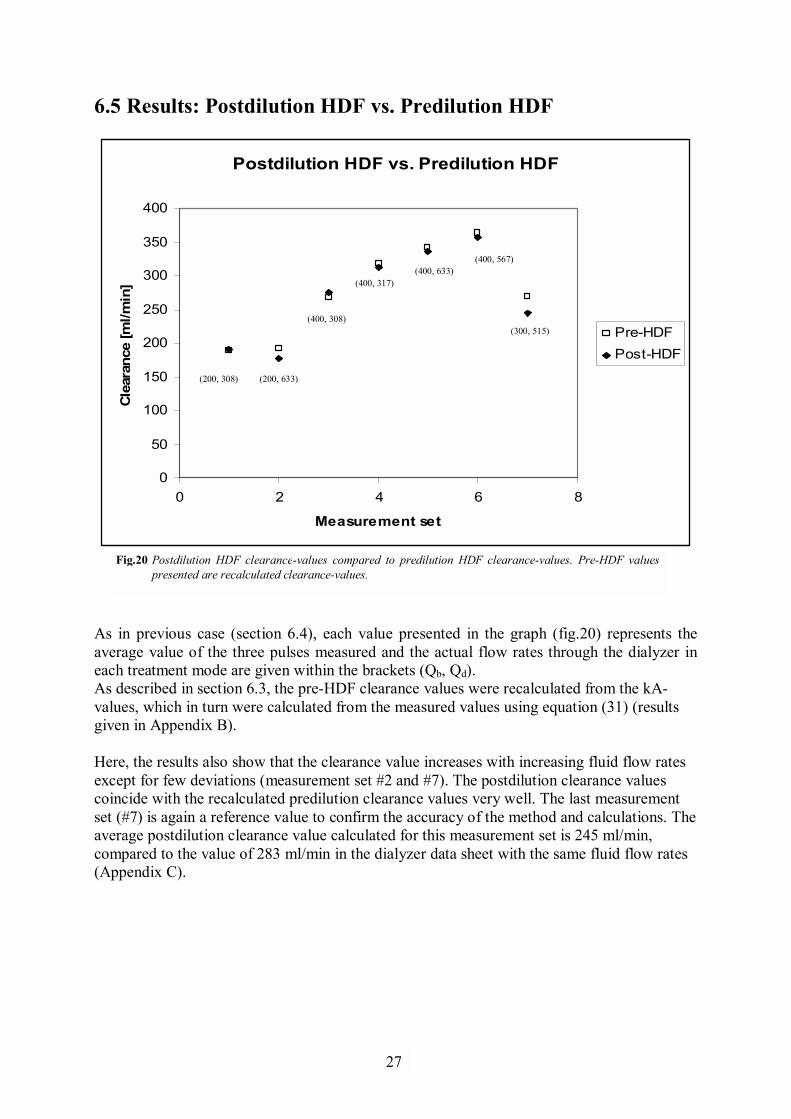
As in previous case (section 6.4), each value presented in the graph (fig.20) represents the average value of the three pulses measured and the actual flow rates through the dialyzer in each treatment mode are given within the brackets (Qb, Qd). As described in section 6.3, the pre-HDF clearance values were recalculated from the kA-values, which in turn were calculated from the measured values using equation (31) (results given in Appendix B). Here, the results also show that the clearance value increases with increasing fluid flow rates except for few deviations (measurement set #2 and #7). The postdilution clearance values coincide with the recalculated predilution clearance values very well. The last measurement set (#7) is again a reference value to confirm the accuracy of the method and calculations. The average postdilution clearance value calculated for this measurement set is 245 ml/min, compared to the value of 283 ml/min in the dialyzer data sheet with the same fluid flow rates (Appendix C).

Fig.20 Postdilution HDF clearance-values compared to predilution HDF clearance-values. Pre-HDF valuespresented are recalculated clearance-values.

(200, 308) (200, 633)

(400, 308)

(400, 317)(400, 633)

(300, 515)

(400, 567)

27

1

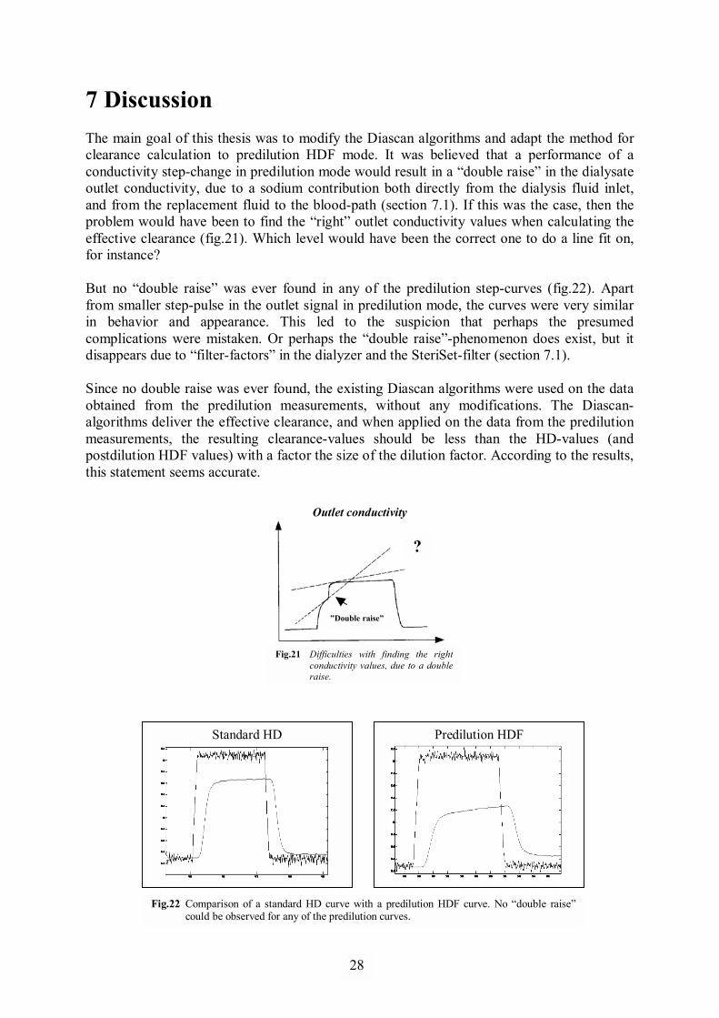
7 Discussion The main goal of this thesis was to modify the Diascan algorithms and adapt the method for clearance calculation to predilution HDF mode. It was believed that a performance of a conductivity step-change in predilution mode would result in a �double raise� in the dialysate outlet conductivity, due to a sodium contribution both directly from the dialysis fluid inlet, and from the replacement fluid to the blood-path (section 7.1). If this was the case, then the problem would have been to find the �right� outlet conductivity values when calculating the effective clearance (fig.21). Which level would have been the correct one to do a line fit on, for instance? But no �double raise� was ever found in any of the predilution step-curves (fig.22). Apart from smaller step-pulse in the outlet signal in predilution mode, the curves were very similar in behavior and appearance. This led to the suspicion that perhaps the presumed complications were mistaken. Or perhaps the �double raise�-phenomenon does exist, but it disappears due to �filter-factors� in the dialyzer and the SteriSet-filter (section 7.1). Since no double raise was ever found, the existing Diascan algorithms were used on the data obtained from the predilution measurements, without any modifications. The Diascan-algorithms deliver the effective clearance, and when applied on the data from the predilution measurements, the resulting clearance-values should be less than the HD-values (and postdilution HDF values) with a factor the size of the dilution factor. According to the results, this statement seems accurate.

Outlet conductivity

Standard HD Predilution HDF

�Double raise�

?

Fig.21 Difficulties with finding the right conductivity values, due to a double raise.

Fig.22 Comparison of a standard HD curve with a predilution HDF curve. No �double raise�could be observed for any of the predilution curves.

28

1

κdi2

κdi1

κdi1

κdi2

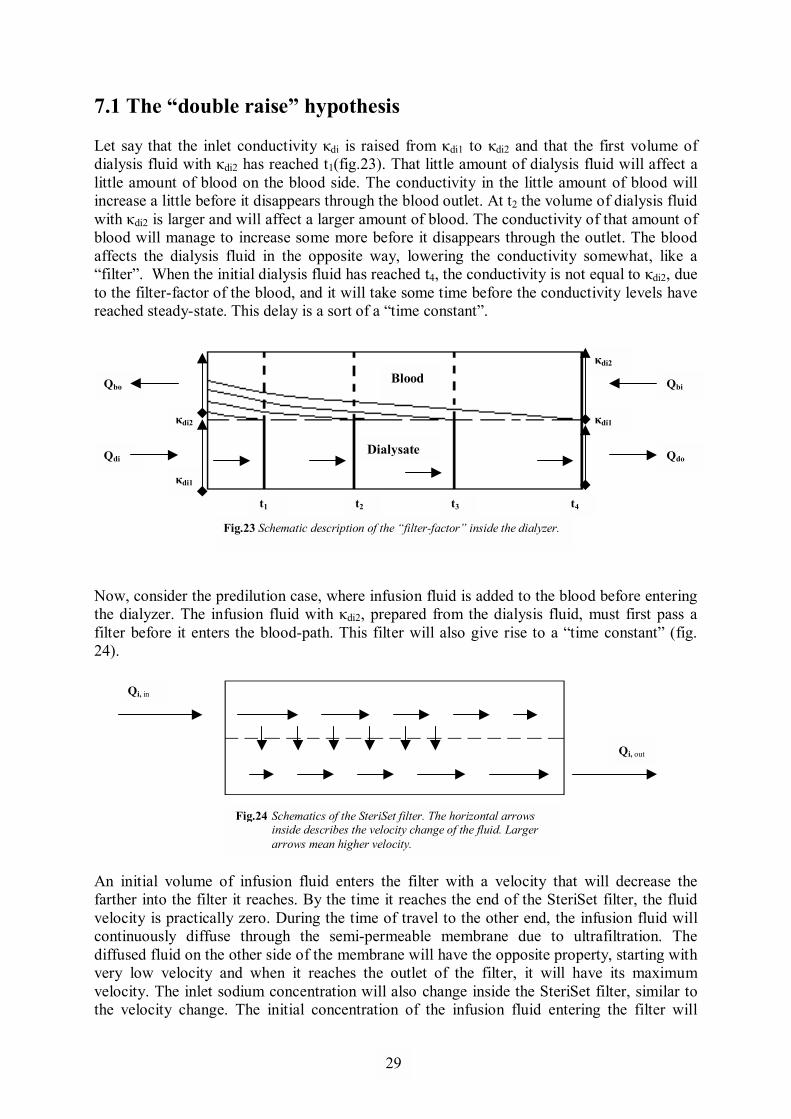
7.1 The �double raise� hypothesis Let say that the inlet conductivity κdi is raised from κdi1 to κdi2 and that the first volume of dialysis fluid with κdi2 has reached t1(fig.23). That little amount of dialysis fluid will affect a little amount of blood on the blood side. The conductivity in the little amount of blood will increase a little before it disappears through the blood outlet. At t2 the volume of dialysis fluid with κdi2 is larger and will affect a larger amount of blood. The conductivity of that amount of blood will manage to increase some more before it disappears through the outlet. The blood affects the dialysis fluid in the opposite way, lowering the conductivity somewhat, like a �filter�. When the initial dialysis fluid has reached t4, the conductivity is not equal to κdi2, due to the filter-factor of the blood, and it will take some time before the conductivity levels have reached steady-state. This delay is a sort of a �time constant�.

Now, consider the predilution case, where infusion fluid is added to the blood before entering the dialyzer. The infusion fluid with κdi2, prepared from the dialysis fluid, must first pass a filter before it enters the blood-path. This filter will also give rise to a �time constant� (fig. 24).

An initial volume of infusion fluid enters the filter with a velocity that will decrease the farther into the filter it reaches. By the time it reaches the end of the SteriSet filter, the fluid velocity is practically zero. During the time of travel to the other end, the infusion fluid will continuously diffuse through the semi-permeable membrane due to ultrafiltration. The diffused fluid on the other side of the membrane will have the opposite property, starting with very low velocity and when it reaches the outlet of the filter, it will have its maximum velocity. The inlet sodium concentration will also change inside the SteriSet filter, similar to the velocity change. The initial concentration of the infusion fluid entering the filter will

Fig.24 Schematics of the SteriSet filter. The horizontal arrows inside describes the velocity change of the fluid. Larger arrows mean higher velocity.

Qi, in

Qi, out

Qbi

Qdo

Qbo

Qdi

t1 t2 t3 t4

Fig.23 Schematic description of the �filter-factor� inside the dialyzer.

Blood

Dialysate

29

1

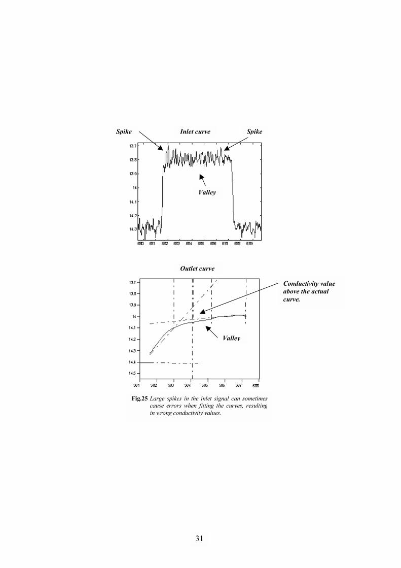
decrease the farther into the filter it reaches, while the diffused fluid will have a higher concentration the closer the outlet it gets. However, when the fluids on both side reaches the point where their relative speeds are switched, sodium will re-diffuse back through the membrane due to the concentration difference around the membrane, thereby causing a time delay for the conductivity raise. This time delay can be approximated by t = V/Q, assuming perfect fluid mixture in the filter. V is the total volume of the filter and Q is the fluid flow. Now, look at the contributions from both the infusion fluid and the dialysis fluid. When the infusion fluid with a conductivity equals κdi2 enters the dialyzer, it will affect the dialysis fluid on the other side of the membrane in the same way as described above, assuming that the infusion fluid and the dialysis fluid (with κdi1) have different sources. When both the dialysis fluid and the infusion fluid with κdi2 are present, the effect of the dialysate outlet conductivity from both fluids, should add up. But due to the time constant in the SteriSet filter, the infusion fluid should be somewhat delayed compared to the dialysis fluid, hence, the �double raise�. Why this phenomenon was never found, could have its explanation in the fact that the two time constants described above probably cancel each other out, or that a small difference in timing would probably be hidden by the filtering effect of the time constants. 7.2 HD vs. Pre-HDF These measurements were meant as a confirmation that the existing Diascan-algorithms were working properly. It is clearly from the results in section 6.4, that the clearance value increases with increasing fluid flow rates. The clearance-value should always be a little bit lower than the blood flow rate used. In predilution measurements, the difference between the blood flow rate and the clearance-value are a bit higher than in standard HD, due to dilution of the blood. For standard HD reference values, see Appendix C. 7.3 Post-HDF vs. Pre-HDF A direct comparison made between the postdilution clearance-values and the recalculated predilution clearance-values shows a very close agreement, with exception of few deviations (see Appendix B). The algorithms have sometimes difficulties in fitting the curves when there are, for instance, spikes larger than the �average� fluctuations in the inlet signal (fig.25). In cases like that, the algorithms could end up using data outside the curve, which would explain the deviant values. The close agreement between the postdilution and the recalculated predilution clearance-values, also confirms the accuracy of the theoretical formula given by equation (21).

30

1

Inlet curveSpike Spike

Outlet curve

Fig.25 Large spikes in the inlet signal can sometimes cause errors when fitting the curves, resultingin wrong conductivity values.

Valley

Valley

Conductivity value above the actual curve.

31

1

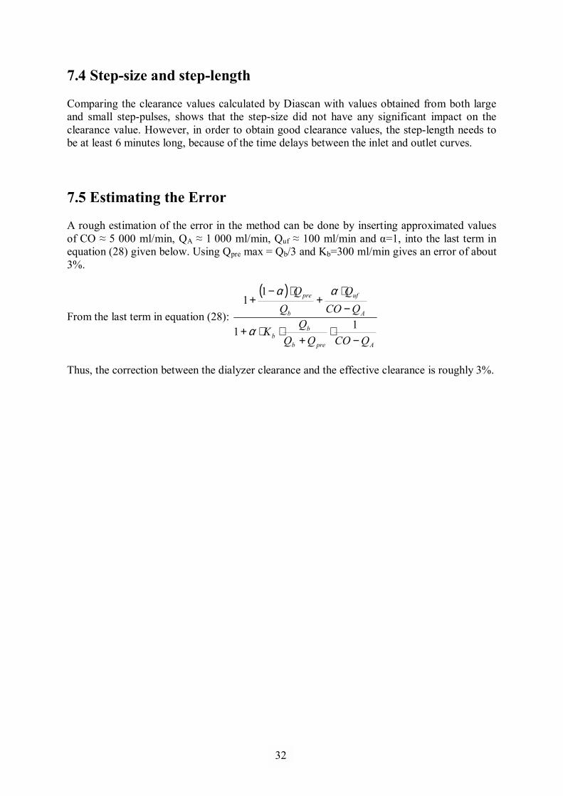
7.4 Step-size and step-length Comparing the clearance values calculated by Diascan with values obtained from both large and small step-pulses, shows that the step-size did not have any significant impact on the clearance value. However, in order to obtain good clearance values, the step-length needs to be at least 6 minutes long, because of the time delays between the inlet and outlet curves. 7.5 Estimating the Error A rough estimation of the error in the method can be done by inserting approximated values of CO ≈ 5 000 ml/min, QA ≈ 1 000 ml/min, Quf ≈ 100 ml/min and α=1, into the last term in equation (28) given below. Using Qpre max = Qb/3 and Kb=300 ml/min gives an error of about 3%.

From the last term in equation (28):

( )

Apreb

bb

A

uf

b

pre

QCOQQQ

K

QCOQ

QQ

−⋅

+⋅⋅+

−⋅

+⋅−

+

11

11

α

αα

Thus, the correction between the dialyzer clearance and the effective clearance is roughly 3%.

32

1

8 Conclusions Judging from the results, the existing Diascan feature also works for predilution HDF mode, without requiring any modifications of the algorithms. The step-size does not have any significant impact on the clearance value. Raising the conductivity by 0.5 mS/cm, and holding the pulse for at least 6 min, gives an adequate value. Results from comparison between the postdilution and the predilution clearance-values, also confirms the accuracy of the theoretical formula given by equation (21). However, more tests and measurements need to be done in order to obtain more statistically significant data.

9 Future Works The natural step for following up this study is to perform the measurements again using bovine blood instead of dialysis solution. Tests with different types of dialyzer and dialysis concentrates must also be done. The measurements showed heavy fluctuations in the dialysate inlet conductivity signal. These fluctuations needs to be minimized in order to minimize the margin of error and improve the accuracy of the clearance values calculated.

33

1

References [1] Daugirdas JT, Blake PG, Ing TS; 2007; Handbook of Dialysis 4th Ed.; Lippincott

Williams & Wilkins; ISBN-13: 978-0-7817-5253-4; ISBN-10: 0-7817-5253-1. [2] Jacobson B; 2006; Medicin och Teknik 5th Ed.; Studentlitteratur; ISBN: 91-44-04760-6. [3] Petitclerc T, Béné B, Jacobs C, Jaudon MC, Goux N; 1995; Non-invasive monitoring of

effective dialysis dose delivered to the Haemodialysis patient; Nephrol.Dial. Transplant; 10: 212-216.

[4] Hörl WH, Lindsay RM, Koch KM, Ronco C, Winchester JF; 2004; Replacement of

Renal Function by Dialysis 5th Rev.Ed; Kluwer Academic Publishers; ISBN: 1-4020-0083-9.

[5] Schneider H, Streicher E; 1985; Mass Transfer Characterization of a New Polysulfone

Membrane; Artif. Organs; 2:180-3. [6] Gotch FA, Sargent JA; 1985; A mechanistic analysis of the National Cooperative

Dialysis Study (NCDS); Kidney Int.; 28: 526-34. [7] Petitclerc T; 2006; Do dialysate conductivity measurements provide conductivity

clearance or ionic dialysance?; Kidney Int.; 70(10):1682-6. [8] Di Filippo S, Pozzoni P, Manzoni C, Andrulli S, Pontoriero G, Locatelli F; 2005;

Relationship between urea clearance and ionic dialysance determined using a single-step conductivity profile; Kidney Int.; 68(5):2389-95.

[9] Petitclerc T, Goux N, Reynier AL, Béné B; 1993; A model for non-invasive estimation

of in vivo Dialyzer performances and patient�s conductivity during hemodialysis; Int. J. Artif. Organs; 16: 8: 585-591.

[10] Ross SM, Uvelli DA, Babb AL; 1973; A One-Dimensional Mathematical Model of

Transmembrane Diffusional and Convective Mass Transfer in a Hemodialyzer; Am. Soc. Mech. Eng. paper n.73WA/Bio 14. Winter Annual Meet, Detroit.

[11] Locatelli F, Di Filippo S, Manzoni C; 2000; Relevance of the conductivity kinetic model

in the control of sodium pool; Kidney Int.; 58(76):89-95. [12] Wolf AV, Brown MG, Prentiss PG; 1980; Concentrative properties of aqueous

solutions: Conversion table. In: Weast RC, Astle MJ, editors; CRC Handbook of Chemistry and Physics 60th Ed.; Boca Raton: CRC Press Inc. ISBN: 0-8493-0460-8.

[13] Sargent JA, Gotch FA; 1983; Principles and biophysics of dialysis. In: Drukker W,

Parsons FM, Maher JF, eds. Replacement of Renal Function by Dialysis, 2nd ed.; Boston: Martinus Nijhoff Publishers; 53-96.

34

1

[14] Jansson O, Persson R, Sternby JP; 2005; Method for conductivity calculation in a treatment fluid upstream and downstream a filtration unit in apparatuses for the blood treatment; US Patent Application Publication; Pub. No.: US 2007/0131595 A1. Pub. Date.: Jun. 14, 2007.

[15] Waniewski J, Werynski A, Ahrenholz P, Lucjanek P, Judycki W, Esther G; 1991;

Theoretical Basis and Experimental Verification of the Impact of Ultrafiltration on Dialyzer Clearance; Artif. Organs; 15(2):70-77.

[16] Sternby J, Jönsson S, Ledebo I; 1992; Hemodiafiltration: Technical Aspects; In:

Shaldon S, Koch KM (eds); Polyamide � The Evolution of a Synthetic Membrane for Renal Therapy; Contrib. Nephrol.; Basel, Karger; (96)86-98.

[17] Sternby J; 2002; Calculations for blood access flow measurements; PM 020715, Internal

Report, Gambro Lundia AB.

35

1

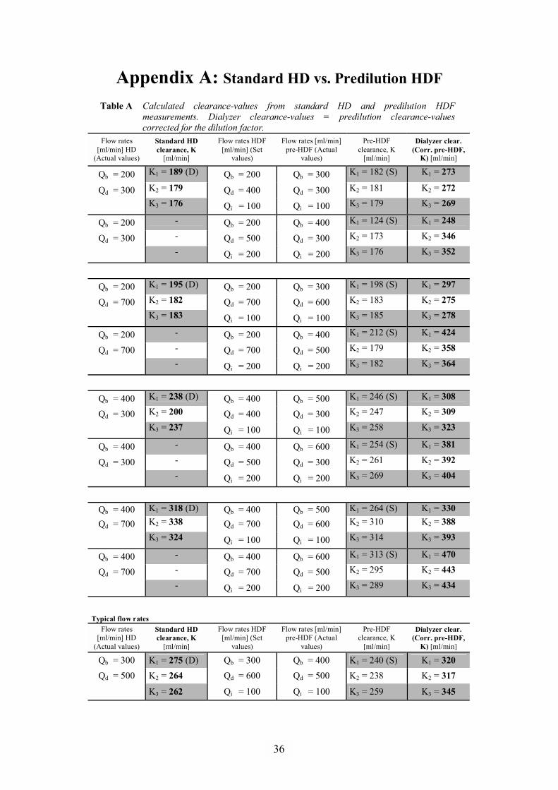
Appendix A: Standard HD vs. Predilution HDF Table A Calculated clearance-values from standard HD and predilution HDF

measurements. Dialyzer clearance-values = predilution clearance-values corrected for the dilution factor.

Flow rates [ml/min] HD

(Actual values)

Standard HD clearance, K

[ml/min]

Flow rates HDF [ml/min] (Set

values)

Flow rates [ml/min] pre-HDF (Actual

values)

Pre-HDF clearance, K

[ml/min]

Dialyzer clear. (Corr. pre-HDF,

K) [ml/min]

Qb = 200 K1 = 189 (D) Qb = 200 Qb = 300 K1 = 182 (S) K1 = 273

Qd = 300 K2 = 179 Qd = 400 Qd = 300 K2 = 181 K2 = 272

K3 = 176 Qi = 100 Qi = 100 K3 = 179 K3 = 269

Qb = 200 - Qb = 200 Qb = 400 K1 = 124 (S) K1 = 248

Qd = 300 - Qd = 500 Qd = 300 K2 = 173 K2 = 346

- Qi = 200 Qi = 200 K3 = 176 K3 = 352

Qb = 200 K1 = 195 (D) Qb = 200 Qb = 300 K1 = 198 (S) K1 = 297

Qd = 700 K2 = 182 Qd = 700 Qd = 600 K2 = 183 K2 = 275

K3 = 183 Qi = 100 Qi = 100 K3 = 185 K3 = 278

Qb = 200 - Qb = 200 Qb = 400 K1 = 212 (S) K1 = 424

Qd = 700 - Qd = 700 Qd = 500 K2 = 179 K2 = 358

- Qi = 200 Qi = 200 K3 = 182 K3 = 364

Qb = 400 K1 = 238 (D) Qb = 400 Qb = 500 K1 = 246 (S) K1 = 308

Qd = 300 K2 = 200 Qd = 400 Qd = 300 K2 = 247 K2 = 309

K3 = 237 Qi = 100 Qi = 100 K3 = 258 K3 = 323

Qb = 400 - Qb = 400 Qb = 600 K1 = 254 (S) K1 = 381

Qd = 300 - Qd = 500 Qd = 300 K2 = 261 K2 = 392

- Qi = 200 Qi = 200 K3 = 269 K3 = 404

Qb = 400 K1 = 318 (D) Qb = 400 Qb = 500 K1 = 264 (S) K1 = 330

Qd = 700 K2 = 338 Qd = 700 Qd = 600 K2 = 310 K2 = 388

K3 = 324 Qi = 100 Qi = 100 K3 = 314 K3 = 393

Qb = 400 - Qb = 400 Qb = 600 K1 = 313 (S) K1 = 470

Qd = 700 - Qd = 700 Qd = 500 K2 = 295 K2 = 443

- Qi = 200 Qi = 200 K3 = 289 K3 = 434

Typical flow rates

Flow rates [ml/min] HD

(Actual values)

Standard HD clearance, K

[ml/min]

Flow rates HDF [ml/min] (Set

values)

Flow rates [ml/min] pre-HDF (Actual

values)

Pre-HDF clearance, K

[ml/min]

Dialyzer clear. (Corr. pre-HDF,

K) [ml/min]

Qb = 300 K1 = 275 (D) Qb = 300 Qb = 400 K1 = 240 (S) K1 = 320 Qd = 500 K2 = 264 Qd = 600 Qd = 500 K2 = 238 K2 = 317

K3 = 262 Qi = 100 Qi = 100 K3 = 259 K3 = 345

36

1

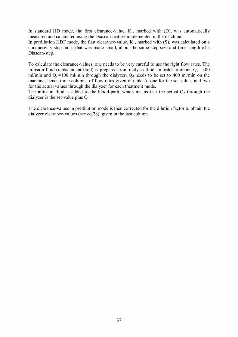
In standard HD mode, the first clearance-value, K1, marked with (D), was automatically measured and calculated using the Diascan feature implemented in the machine. In predilution HDF mode, the first clearance-value, K1, marked with (S), was calculated on a conductivity-step pulse that was made small, about the same step-size and time-length of a Diascan-step. To calculate the clearance-values, one needs to be very careful to use the right flow rates. The infusion fluid (replacement fluid) is prepared from dialysis fluid. In order to obtain Qd =300 ml/min and Qi =100 ml/min through the dialyzer, Qd needs to be set to 400 ml/min on the machine, hence three columns of flow rates given in table A, one for the set values and two for the actual values through the dialyzer for each treatment mode. The infusion fluid is added to the blood-path, which means that the actual Qb through the dialyzer is the set-value plus Qi. The clearance-values in predilution mode is then corrected for the dilution factor to obtain the dialyzer clearance-values (see eq.28), given in the last column.

37

1

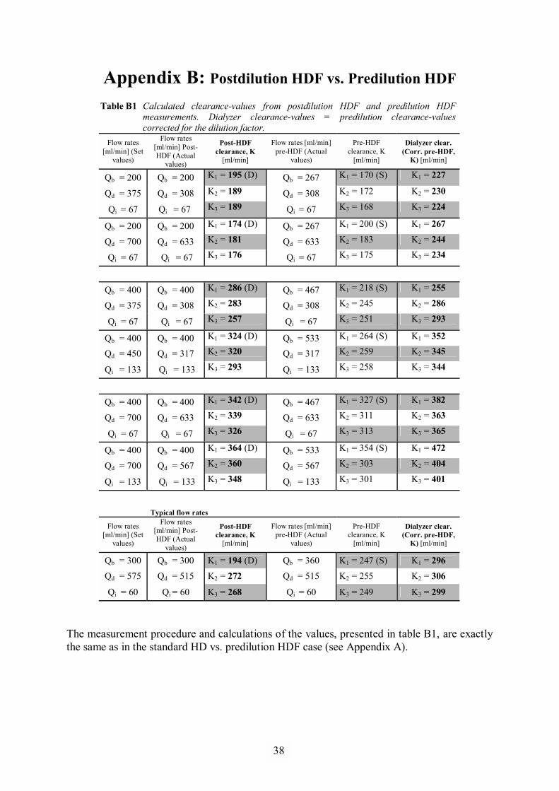
Appendix B: Postdilution HDF vs. Predilution HDF Table B1 Calculated clearance-values from postdilution HDF and predilution HDF

measurements. Dialyzer clearance-values = predilution clearance-values corrected for the dilution factor.

Flow rates [ml/min] (Set

values)

Flow rates [ml/min] Post-HDF (Actual

values)

Post-HDF clearance, K

[ml/min]

Flow rates [ml/min] pre-HDF (Actual

values)

Pre-HDF clearance, K

[ml/min]

Dialyzer clear. (Corr. pre-HDF,

K) [ml/min]

Qb = 200 Qb = 200 K1 = 195 (D) Qb = 267 K1 = 170 (S) K1 = 227

Qd = 375 Qd = 308 K2 = 189 Qd = 308 K2 = 172 K2 = 230

Qi = 67 Qi = 67 K3 = 189 Qi = 67 K3 = 168 K3 = 224

Qb = 200 Qb = 200 K1 = 174 (D) Qb = 267 K1 = 200 (S) K1 = 267

Qd = 700 Qd = 633 K2 = 181 Qd = 633 K2 = 183 K2 = 244

Qi = 67 Qi = 67 K3 = 176 Qi = 67 K3 = 175 K3 = 234

Qb = 400 Qb = 400 K1 = 286 (D) Qb = 467 K1 = 218 (S) K1 = 255

Qd = 375 Qd = 308 K2 = 283 Qd = 308 K2 = 245 K2 = 286

Qi = 67 Qi = 67 K3 = 257 Qi = 67 K3 = 251 K3 = 293

Qb = 400 Qb = 400 K1 = 324 (D) Qb = 533 K1 = 264 (S) K1 = 352

Qd = 450 Qd = 317 K2 = 320 Qd = 317 K2 = 259 K2 = 345

Qi = 133 Qi = 133 K3 = 293 Qi = 133 K3 = 258 K3 = 344

Qb = 400 Qb = 400 K1 = 342 (D) Qb = 467 K1 = 327 (S) K1 = 382

Qd = 700 Qd = 633 K2 = 339 Qd = 633 K2 = 311 K2 = 363

Qi = 67 Qi = 67 K3 = 326 Qi = 67 K3 = 313 K3 = 365

Qb = 400 Qb = 400 K1 = 364 (D) Qb = 533 K1 = 354 (S) K1 = 472

Qd = 700 Qd = 567 K2 = 360 Qd = 567 K2 = 303 K2 = 404

Qi = 133 Qi = 133 K3 = 348 Qi = 133 K3 = 301 K3 = 401

Typical flow rates

Flow rates [ml/min] (Set

values)

Flow rates [ml/min] Post-HDF (Actual

values)

Post-HDF clearance, K

[ml/min]

Flow rates [ml/min] pre-HDF (Actual

values)

Pre-HDF clearance, K

[ml/min]

Dialyzer clear. (Corr. pre-HDF,

K) [ml/min]

Qb = 300 Qb = 300 K1 = 194 (D) Qb = 360 K1 = 247 (S) K1 = 296

Qd = 575 Qd = 515 K2 = 272 Qd = 515 K2 = 255 K2 = 306

Qi = 60 Qi = 60 K3 = 268 Qi = 60 K3 = 249 K3 = 299

The measurement procedure and calculations of the values, presented in table B1, are exactly the same as in the standard HD vs. predilution HDF case (see Appendix A).

38

1

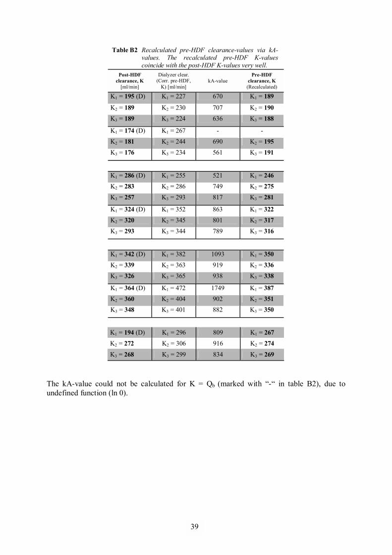
Table B2 Recalculated pre-HDF clearance-values via kA-values. The recalculated pre-HDF K-values coincide with the post-HDF K-values very well.

Post-HDF clearance, K

[ml/min]

Dialyzer clear. (Corr. pre-HDF,

K) [ml/min] kA-value

Pre-HDF clearance, K (Recalculated)

K1 = 195 (D) K1 = 227 670 K1 = 189

K2 = 189 K2 = 230 707 K2 = 190

K3 = 189 K3 = 224 636 K3 = 188

K1 = 174 (D) K1 = 267 - -

K2 = 181 K2 = 244 690 K2 = 195

K3 = 176 K3 = 234 561 K3 = 191

K1 = 286 (D) K1 = 255 521 K1 = 246

K2 = 283 K2 = 286 749 K2 = 275

K3 = 257 K3 = 293 817 K3 = 281

K1 = 324 (D) K1 = 352 863 K1 = 322

K2 = 320 K2 = 345 801 K2 = 317

K3 = 293 K3 = 344 789 K3 = 316

K1 = 342 (D) K1 = 382 1093 K1 = 350

K2 = 339 K2 = 363 919 K2 = 336

K3 = 326 K3 = 365 938 K3 = 338

K1 = 364 (D) K1 = 472 1749 K1 = 387

K2 = 360 K2 = 404 902 K2 = 351 K3 = 348 K3 = 401 882 K3 = 350

K1 = 194 (D) K1 = 296 809 K1 = 267

K2 = 272 K2 = 306 916 K2 = 274

K3 = 268 K3 = 299 834 K3 = 269

The kA-value could not be calculated for K = Qb (marked with �-� in table B2), due to undefined function (ln 0).

39

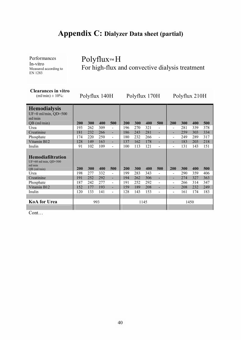
1

Appendix C: Dialyzer Data sheet (partial)

Polyflux� H For high-flux and convective dialysis treatment

Clearances in vitro

(ml/min) ± 10%:

Polyflux 140H Polyflux 170H Polyflux 210H

Hemodialysis UF=0 ml/min, QD=500 ml/min QB (ml/min) 200 300 400 500 200 300 400 500 200 300 400 500 Urea 193 262 309 - 196 270 321 - - 281 339 378 Creatinine 181 232 266 - 186 243 281 - - 259 303 334 Phosphate 174 220 250 - 180 232 266 - - 249 289 317 Vitamin B12 128 149 163 - 137 162 178 - - 183 203 218 Inulin 91 102 109 - 100 113 121 - - 131 143 151

Hemodiafiltration UF=60 ml/min, QD=500 ml/min QB (ml/min) 200 300 400 500 200 300 400 500 200 300 400 500 Urea 198 277 332 - 199 283 343 - - 290 359 406 Creatinine 191 252 292 - 194 262 306 - - 274 327 363 Phosphate 187 242 277 - 191 252 292 - - 266 314 347 Vitamin B12 152 177 193 - 159 189 208 - - 208 232 249 Inulin 120 133 141 - 128 143 153 - - 161 174 183 KoA for Urea 993 1145 1450 Cont�

Performances In-vitro Measured according to EN 1283

40

TRITA-CSC-E 2009:075 ISRN-KTH/CSC/E--09/075--SE

ISSN-1653-5715

www.kth.se