CONDITION HEALTH MONITORING AND ITS … DETECTION/CHARACTERIZATION WITHIN HYDROPOWER TURBINES by ......
195
CONDITION HEALTH MONITORING AND ITS APPLICATION TO CAVITATION DETECTION/CHARACTERIZATION WITHIN HYDROPOWER TURBINES by Samuel J. Dyas
-
Upload
phungkhanh -
Category
Documents
-
view
217 -
download
1
Transcript of CONDITION HEALTH MONITORING AND ITS … DETECTION/CHARACTERIZATION WITHIN HYDROPOWER TURBINES by ......

CONDITION HEALTH MONITORING AND ITS APPLICATION TO
CAVITATION DETECTION/CHARACTERIZATION
WITHIN HYDROPOWER TURBINES
by
Samuel J. Dyas

Copyright by Samuel J. Dyas 2013
All Rights Reserved

ii
A thesis submitted to the Faculty and the Board of Trustees of the Colorado School of
Mines in partial fulfillment of the requirements for the degree of Masters of Science (Mechanical
Engineering).
Golden, Colorado
Date _____________________
Signed: ____________________________
Samuel J. Dyas
Signed: ____________________________
Dr. Michael A. Mooney
Thesis Advisor
Golden, Colorado
Date _____________________
Signed: ____________________________
Dr. Greg Jackson
Professor and Head of
Department of Mechanical Engineering
iii
ABSTRACT
Hydroelectric power has been the number one renewable energy source in the U.S. since
the beginning of the industrial revolution and continues to be today. Hydroelectricity is a critical
component in the power production grid to keep greenhouse gas emissions and pollution
minimized. As such, it is crucial that unexpected shutdowns and unplanned maintenance of
hydropower turbines be kept to a minimum, so as to maximize hydroelectricity production.
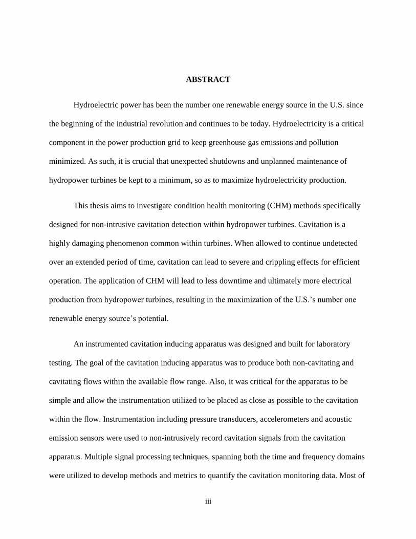
This thesis aims to investigate condition health monitoring (CHM) methods specifically
designed for non-intrusive cavitation detection within hydropower turbines. Cavitation is a
highly damaging phenomenon common within turbines. When allowed to continue undetected
over an extended period of time, cavitation can lead to severe and crippling effects for efficient
operation. The application of CHM will lead to less downtime and ultimately more electrical
production from hydropower turbines, resulting in the maximization of the U.S.’s number one
renewable energy source’s potential.
An instrumented cavitation inducing apparatus was designed and built for laboratory
testing. The goal of the cavitation inducing apparatus was to produce both non-cavitating and
cavitating flows within the available flow range. Also, it was critical for the apparatus to be
simple and allow the instrumentation utilized to be placed as close as possible to the cavitation
within the flow. Instrumentation including pressure transducers, accelerometers and acoustic
emission sensors were used to non-intrusively record cavitation signals from the cavitation
apparatus. Multiple signal processing techniques, spanning both the time and frequency domains
were utilized to develop methods and metrics to quantify the cavitation monitoring data. Most of
iv
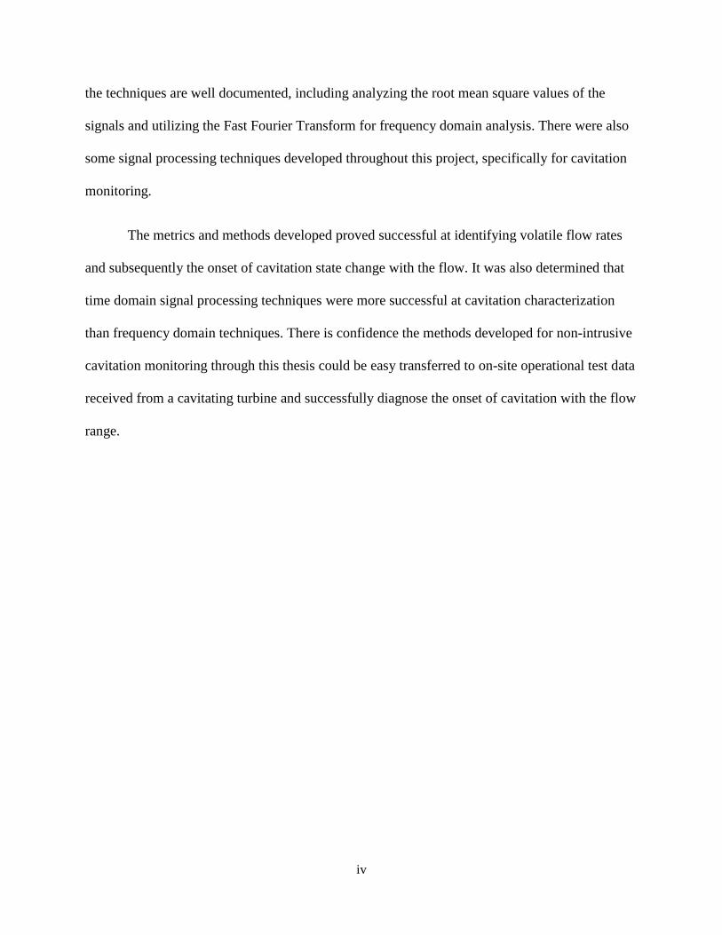
the techniques are well documented, including analyzing the root mean square values of the
signals and utilizing the Fast Fourier Transform for frequency domain analysis. There were also
some signal processing techniques developed throughout this project, specifically for cavitation
monitoring.
The metrics and methods developed proved successful at identifying volatile flow rates
and subsequently the onset of cavitation state change with the flow. It was also determined that
time domain signal processing techniques were more successful at cavitation characterization
than frequency domain techniques. There is confidence the methods developed for non-intrusive
cavitation monitoring through this thesis could be easy transferred to on-site operational test data
received from a cavitating turbine and successfully diagnose the onset of cavitation with the flow
range.
v
TABLE OF CONTENTS
ABSTRACT ................................................................................................................................... iii
TABLE OF CONTENTS .................................................................................................................v
LIST OF FIGURES ....................................................................................................................... ix
LIST OF TABLES ...................................................................................................................... xvii
ACNKOWLEDGEMENTS ....................................................................................................... xviii
CHAPTER 1 INTRODUCTION .................................................................................................1
1.1 Background ..................................................................................................................1
1.2 Summary ......................................................................................................................2
CHAPTER 2 LITERATURE REVIEW ......................................................................................4
2.1 Hydropower Plant Basics .............................................................................................4
2.2 Hydropower Turbine Basics ........................................................................................5
2.3 Cavitation Erosion .......................................................................................................6
2.4 Previous Research ........................................................................................................9
2.4.1 Example Case Study ..................................................................................................11
CHAPTER 3 FUNDAMENTAL RESEARCH QUESTIONS, GOALS AND PURPOSE ......17
3.1 Fundamental Research Questions ..............................................................................17
3.2 Project Objectives ......................................................................................................18
CHAPTER 4 EXPERIMENTAL SET-UP ................................................................................19
4.1 Design Conception .....................................................................................................19
4.2 Design ........................................................................................................................21
CHAPTER 5 INSTRUMENTATION AND DATA ANALYSIS METHODS ........................28
5.1 Sensors .......................................................................................................................28
5.1.1 Pressure Sensor ..........................................................................................................28
5.1.2 Accelerometers ..........................................................................................................29
vi
5.1.3 Acoustic Emission Sensor..........................................................................................30
5.2 Hardware ....................................................................................................................31
5.3 Software .....................................................................................................................31
5.4 Data Acquisition Parameters......................................................................................32
5.5 Band-Pass Filtering ....................................................................................................32
5.6 Data Analysis Background ........................................................................................33
5.6.1 Root-Mean Square Signal Analysis ...........................................................................34
5.6.2 Auto-Correlation ........................................................................................................35
5.6.3 Spike Analysis ............................................................................................................35
5.6.4 Burst Analysis ............................................................................................................36
5.6.5 Coherence Analysis ...................................................................................................37
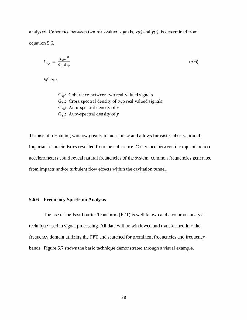
5.6.6 Frequency Spectrum Analysis ...................................................................................38
5.6.7 Normalized Frequency Spectrum Analysis ...............................................................39
CHAPTER 6 RESULTS ............................................................................................................41
6.1 Testing Procedure and Testing Days .........................................................................41
6.2 Gage Pressure and Cavitation Index versus Flow Rate .............................................44
6.3 Root-Mean-Square Signal Strength Analysis ............................................................48
6.4 Auto-Correlation of Signals .......................................................................................51
6.5 Frequency Spectrum Analysis ...................................................................................55
6.6 Normalized Frequency Spectrum Analysis ...............................................................60
6.7 Coherence between Top and Bottom Acceleration ...................................................65
6.8 Spike Analysis ............................................................................................................68
6.9 Burst Analysis ............................................................................................................71
vii
CHAPTER 7 CONCLUSIONS AND RECOMMENDATIONS FOR FUTURE WORK .......74
7.1 Conclusions ................................................................................................................74
7.2 Future Work ...............................................................................................................76
LIST OF ABBREVIATIONS AND SYMBOLS ..........................................................................77
REFERENCES ..............................................................................................................................79
APPENDIX A PREDICTIVE CAVITATION INDEX MATLAB© CODE ..............................82
APPENDIX B VISUAL OF CAVITATION INDEXES.............................................................83
APPENDIX C REYNOLDS NUMBER CALCULATIONS ......................................................84
APPENDIX D FINAL TECHNICAL DRAWINGS AND ISOMETRIC VIEWS OF CAD
MODEL OF CAVITATION TUNNEL.........................................................................................85
APPENDIX E DETAILED PHOTOS OF FINAL EXPERIMENTAL SET-UP ........................94
APPENDIX F BAND-PASS FILTER DESIGN FOR POST SIGNAL PROCESSING ............98
APPENDIX G EXAMPLE BURST ANALYSIS MATLAB© CODE ....................................100
APPENDIX H EXAMPLE FREQUENCY SPECTRUM NORMALIZATION MATLAB©
CODE ...........................................................................................................................................101
APPENDIX I LIST OF TESTING DAYS AND CORRESPONDING ATMOSPHERIC
PRESSURES................................................................................................................................103
APPENDIX J MATLAB© CODE FOR DETERMING AVERAGE ERROR BETWEEN
INCREASING AND DECREASING FLOW RATE VERSUS CAVITATION INDEX POWER
REGRESSION .............................................................................................................................104
APPENDIX K CAVITATION AT FLOW – PHOTOS ............................................................105
APPENDIX L PRIMARY MATLAB© CODE FOR SIGNAL ANALYSIS ...........................109
APPENDIX M SUPPLEMENTAL AUTO-CORRELATION PLOTS ....................................116
APPENDIX N SUPPLEMENTAL FREQUENCY SPECTRUM PLOTS ...............................125
APPENDIX O NORMALIZED FREQUENCY SPECTRUM BACKGROUND ....................140
APPENDIX P SUPPLEMENTAL NORMAZLIED FREQUENCY SPECTRUM PLOTS .....142
APPENDIX Q COHERENCE FILTERING EFFECTS ...........................................................157

viii
APPENDIX R SUPPLEMENTAL COHERENCE PLOTS ......................................................161
APPENDIX S AVERAGE SPIKE ANALYSIS PLOTS ..........................................................166
APPENDIX T BURST ANALYSIS PLOTS AND NORMALIZATION BACKGROUND ...168
ix
LIST OF FIGURES
Figure 2.1 Typical Hydropower Plant Set-up [5] ..........................................................................4
Figure 2.2 Francis Turbine Diagram [6] ........................................................................................5
Figure 2.3 Diagram of Cavitation leading to Erosion of Critical Hydro Turbine
Components [7] ................................................................................................................................7
Figure 2.4 Cavitation Damage on a Turbine’s Runner Blade at Fremont Canyon Power Plant
in Wyoming (USBR facility) ...........................................................................................................7
Figure 2.5 Typical Material Mass Loss versus Exposure Time due to Prolonged
Cavitation [10] .................................................................................................................................8
Figure 2.6 Outline of a Francis Turbine indicating the Location and Direction of the
Accelerometers [22] .......................................................................................................................11
Figure 2.7 RMS Output of Vibrations Signals Filtered between 3-6 kHz as a Function of
Output Power [22]..........................................................................................................................12
Figure 2.8 Auto Power Spectra from 1-6 kHz of Shaft Vibrations as a Function of Output
Power [22] ......................................................................................................................................13
Figure 2.9 Auto Power Spectra up to 20 kHz of Guide Bearing Vibrations as a Function of
Output Power [22]..........................................................................................................................13
Figure 2.10 Auto Power Spectra up to 20 kHz of Guide Vane Vibrations as a Function of
Output Power [22]..........................................................................................................................14
Figure 2.11 Auto Power Spectra of Demodulated Filtered Signal (3-6 kHz) for Shaft
Vibrations as a Function of Output Power [22] .............................................................................15
Figure 2.12 Auto Power Spectra of Demodulated Filtered Signal (3-6 kHz) for Guide
Bearing Vibrations as a Function of Output Power [22] ...............................................................15
Figure 2.13 Auto Power Spectra of Demodulated Filtered Signal (3-6 kHz) for Guide
Vane Vibrations as a Function of Output Power [22]....................................................................15
Figure 4.1 USBR Denver Federal Center Hydraulic Laboratory High Head Pump Discharge
Curve ..............................................................................................................................................20
Figure 4.2 Simplified and Generalized Diagram of the USBR Denver Federal Center
Hydraulic Laboratory HHP Station Standard Set-up .....................................................................20
Figure 4.3 Incipient Cavitation Characteristics of Offsets into the Flow [9] .................................22
x
Figure 4.4 Isometric View of Final Rendering of Cavitation Tunnel and Photo of
Cavitation Tunnel In-situ ...............................................................................................................26
Figure 4.5 Side View of Sensor Locations in Cavitation Tunnel ................................................26
Figure 4.6 Pictures of Final Experimental Set-up ........................................................................27
Figure 5.1 View of Cavitation Tunnel with Sensors in Place during Operational Testing .........28
Figure 5.2 Pressure Transducer Calibration Curve ......................................................................29
Figure 5.3 Accelerometer Sensitivity Curve [28] ........................................................................30
Figure 5.4 DECI AE Sensor Sensitivity Curve [29] ....................................................................31
Figure 5.5 General Data Analysis Flow Chart .............................................................................34
Figure 5.6 Example of Ideal Data to be Quantified by Burst analysis ........................................37
Figure 5.7 Fast Fourier Transform Example................................................................................39
Figure 5.8 Spectrum Normalization Visual ................................................................................40
Figure 6.1 Raw Acceleration Data from Bottom of Cavitation Tunnel for Non-Cavitating,
Incipient Cavitation and Developed Cavitating Flow ....................................................................42
Figure 6.2 Raw Acoustic Emission Data from Bottom of Cavitation Tunnel for Non-Cavitating,
Incipient Cavitation and Developed Cavitating Flow ....................................................................43
Figure 6.3 Gage Pressure recorded at Cavitation Inducing Offset into the Flow ........................44
Figure 6.4 Corresponding Cavitation Index to Flow Rate ..........................................................45
Figure 6.5 Visual of Cavitation within Tunnel at Various Flow Rates .......................................47
Figure 6.6 RMS of Acceleration from Top of Tunnel corresponding to Flow Rate ...................49
Figure 6.7 RMS of Acceleration from Bottom of Tunnel corresponding to Flow Rate ..............49
Figure 6.8 RMS of AE Sensor Signal corresponding to Flow Rate .........................................50
Figure 6.9 Auto-Correlation of Top Acceleration at Non-Cavitating, Incipient Cavitation and
Developed Cavitation Flow Rates .................................................................................................52
Figure 6.10 Auto-Correlation of Bottom Acceleration at Non-Cavitating, Incipient Cavitation
and Developed Cavitation Flow Rates ...........................................................................................52
xi
Figure 6.11 Auto-Correlation of Acoustic Emission at Non-Cavitating, Incipient Cavitation
and Developed Cavitation Flow Rates ...........................................................................................54
Figure 6.12 Frequency Spectrum of Acceleration Signal recorded from Top of Cavitation
Tunnel during Non-Cavitating, Incipient Cavitation and Developed Cavitation Flow Rates .......56
Figure 6.13 Frequency Spectrum of Acceleration Signal recorded from Bottom of Cavitation
Tunnel during Non-Cavitating, Incipient Cavitation and Developed Cavitation Flow Rates .......57
Figure 6.14 Frequency Spectrum of Acoustic Emission Signal Recorded from Top of
Cavitation Tunnel during Non-Cavitating, Incipient Cavitation and Developed Cavitation Flow
Rates ...............................................................................................................................................58
Figure 6.15 Normalized Frequency Spectrum of Acceleration Signal recorded from Top of
Cavitation Tunnel during Non-Cavitating, Incipient Cavitation and Developed Cavitation Flow
Rates ...............................................................................................................................................61
Figure 6.16 Normalized Frequency Spectrum of Acceleration Signal recorded from Bottom of
Cavitation Tunnel during Non-Cavitating, Incipient Cavitation and Developed Cavitation Flow
Rates ...............................................................................................................................................62
Figure 6.17 Normalized Frequency Spectrum of Acoustic Emission recorded from Bottom of
Cavitation Tunnel during Non-Cavitating, Incipient Cavitation and Developed Cavitation Flow
Rates ...............................................................................................................................................63
Figure 6.18 Coherence of Top and Bottom Acceleration Readings at Non-Cavitating,
Incipient Cavitation and Developed Cavitation Flow Rates ..........................................................66
Figure 6.19 Spike Analysis of Acceleration Signal Collected from Top of Cavitation Tunnel...68
Figure 6.20 Spike Analysis of Acceleration Signal Collected from Bottom of Cavitation
Tunnel ............................................................................................................................................69
Figure 6.21 Spike Analysis of Acoustic Emission Signal Collected from Bottom of Cavitation
Tunnel ............................................................................................................................................69
Figure 6.22 Burst Analysis of Acceleration Signal Collected from Top of Cavitation
Tunnel ............................................................................................................................................72
Figure 6.23 Burst Analysis of Acceleration Signal Collected from Bottom of Cavitation
Tunnel ............................................................................................................................................72
Figure 6.24 Burst Analysis of Acoustic Emission Collected from Bottom of Cavitation
Tunnel ............................................................................................................................................73
Figure B.1 Visual of Cavitation Index Implications ....................................................................83
xii
Figure C.1 Reynolds Number Calculations .................................................................................84
Figure D.1 Technical Assembly Drawing of Final Cavitation Tunnel Design............................85
Figure D.2 Final Back Plate Design Technical Drawing for Cavitation Tunnel .........................86
Figure D.3 Final Top Plate Design Technical Drawing for Cavitation Tunnel ...........................87
Figure D.4 Final Bottom Plate Design Technical Drawing for Cavitation Tunnel .....................88
Figure D.5 Final Front Plate Design Technical Drawing for Cavitation Tunnel.........................89
Figure D.6 Final Angle Iron Design Technical Drawing for Cavitation Tunnel .........................90
Figure D.7 Top Isometric View of Final CAD Model of Cavitation Tunnel ..............................91
Figure D.8 Bottom Isometric View of Final CAD Model of Cavitation Tunnel .........................92
Figure D.9 Transparent Isometric View of Final Cavitation Tunnel CAD Model .....................93
Figure E.1 Photo of Experimental Set-up 1 .................................................................................94
Figure E.2 Photo of Experimental Set-up 2 .................................................................................95
Figure E.3 Photo of Experimental Set-up 3 .................................................................................95
Figure E.4 Photo of Cavitation Tunnel In-Situ ............................................................................96
Figure E.5 Close-up of Venturi within Experimental Set-up ......................................................96
Figure E.6 Close-up of Variable Frequency Drive Motor and High Head Pump........................97
Figure F.1 Ideal Low Pass Filter Design Supporting Calculations ..............................................98
Figure F.2 Ideal High Pass Filter Design Supporting Calculations .............................................99
Figure K.1 Cavitation at Offset into the Flow at Flow Rates 2.25-3.00 ft3/s.............................105
Figure K.2 Cavitation at Offset into the Flow at Flow Rates 3.25-4.00 ft3/s.............................106
Figure K.3 Cavitation at Offset into the Flow at Flow Rates 4.25-5.00 ft3/s.............................107
Figure K.4 Cavitation at Offset into the Flow at Flow Rates 5.00-5.25 ft3/s.............................108
Figure M.1 Auto-Correlation of Top Acceleration at Flow Rates 2.00-2.50 ft3/s .....................116
Figure M.2 Auto Correlation of Top Acceleration at Flow Rates 2.75-3.25 ft3/s .....................117
Figure M.3 Auto Correlation of Top Acceleration at Flow Rates 4.00, 5.00, 5.25 ft3/s ............118
xiii
Figure M.4 Auto Correlation of Bottom Acceleration at Flow Rates 2.00-2.50 ft3/s ................119
Figure M.5 Auto Correlation of Bottom Acceleration at Flow Rates 2.75-3.25 ft3/s ................120
Figure M.6 Auto Correlation of Bottom Acceleration at Flow Rates 4.00, 5.00, 5.25 ft3/s ......121
Figure M.7 Auto Correlation of Acoustic Emission at Flow Rates 2.00-2.50 ft3/s ...................122
Figure M.8 Auto Correlation of Acoustic Emission at Flow Rates 2.75-3.25 ft3/s ...................123
Figure M.9 Auto Correlation of Acoustic Emission at Flow Rates 4.00, 5.00, 5.25 ft3/s .........124
Figure N.1 Frequency Spectrum of Top Acceleration – Flow Range 2.00 – 2.50 ft3/s .............125
Figure N.2 Frequency Spectrum of Top Acceleration – Flow Range 2.75 – 3.25 ft3/s .............126
Figure N.3 Frequency Spectrum of Top Acceleration – Flow Range 3.50 – 4.00 ft3/s .............127
Figure N.4 Frequency Spectrum of Top Acceleration – Flow Range 4.25 – 4.75 ft3/s .............128
Figure N.5 Frequency Spectrum of Top Acceleration – Flow Range 5.00 – 5.25 ft3/s .............129
Figure N.6 Frequency Spectrum of Bottom Acceleration – Flow Range 2.00 – 2.50 ft3/s .......130
Figure N.7 Frequency Spectrum of Bottom Acceleration – Flow Range 2.75 – 3.25 ft3/s .......131
Figure N.8 Frequency Spectrum of Bottom Acceleration – Flow Range 3.50 – 4.00 ft3/s .......132
Figure N.9 Frequency Spectrum of Bottom Acceleration – Flow Range 4.25 – 4.75 ft3/s .......133
Figure N.10 Frequency Spectrum of Bottom Acceleration – Flow Range 5.00 – 5.25 ft3/s .....134
Figure N.11 Frequency Spectrum of Acoustic Emission – Flow Rates 2.00 – 2.50 ft3/s ..........135
Figure N.12 Frequency Spectrum of Acoustic Emission – Flow Rates 2.75 – 3.25 ft3/s ..........136
Figure N.13 Frequency Spectrum of Acoustic Emission – Flow Rates 3.50 – 4.00 ft3/s ..........137
Figure N.14 Frequency Spectrum of Acoustic Emission – Flow Rates 4.00 – 4.75 ft3/s ..........138
Figure N.15 Frequency Spectrum of Acoustic Emission – Flow Rates 5.00 – 5.25 ft3/s ..........139
Figure O.1 Visual of Creating Reference FFT to be used to Normalize all FFTs .....................140
Figure P.1 Normalized Frequency Spectrum of Top Acceleration – Flow
Rates 2.00 – 2.50 ft3/s ..................................................................................................................142
Figure P.2 Normalized Frequency Spectrum of Top Acceleration – Flow
Rates 2.75 – 3.25 ft3/s ..................................................................................................................143
xiv
Figure P.3 Normalized Frequency Spectrum of Top Acceleration – Flow
Rates 3.50 – 4.00 ft3/s ..................................................................................................................144
Figure P.4 Normalized Frequency Spectrum of Top Acceleration – Flow
Rates 4.25 – 4.75 ft3/s ..................................................................................................................145
Figure P.5 Normalized Frequency Spectrum of Top Acceleration – Flow
Rates 5.00 – 5.25 ft3/s ..................................................................................................................146
Figure P.6 Normalized Frequency Spectrum of Bottom Acceleration – Flow
Rates 2.00 - 2.50 ft3/s ...................................................................................................................147
Figure P.7 Normalized Frequency Spectrum of Bottom Acceleration – Flow
Rates 2.75 - 3.25 ft3/s ...................................................................................................................148
Figure P.8 Normalized Frequency Spectrum of Bottom Acceleration – Flow
Rates 3.50 - 4.00 ft3/s ...................................................................................................................149
Figure P.9 Normalized Frequency Spectrum of Bottom Acceleration – Flow
Rates 4.25 - 4.75 ft3/s ...................................................................................................................150
Figure P.10 Normalized Frequency Spectrum of Bottom Acceleration – Flow
Rates 5.00 - 5.25 ft3/s ...................................................................................................................151
Figure P.11 Normalized Frequency Spectrum of Acoustic Emission – Flow
Rates 2.00 - 2.50 ft3/s ...................................................................................................................152
Figure P.12 Normalized Frequency Spectrum of Acoustic Emission – Flow
Rates 2.75 - 3.25 ft3/s ...................................................................................................................153
Figure P.13 Normalized Frequency Spectrum of Acoustic Emission – Flow
Rates 3.50 - 4.00 ft3/s ...................................................................................................................154
Figure P.14 Normalized Frequency Spectrum of Acoustic Emission – Flow
Rates 4.25 - 4.75 ft3/s ...................................................................................................................155
Figure P.15 Normalized Frequency Spectrum of Acoustic Emission – Flow
Rates 5.00 - 5.25 ft3/s ...................................................................................................................156
Figure Q.1 Computational Time for Coherence Plots with varying Hanning Window
Length ..........................................................................................................................................158
Figure Q.2 Coherence between Top and Bottom Acceleration with Hanning Window of varying
Length 220
– 218
............................................................................................................................159
xv
Figure Q.3 Coherence between Top and Bottom Acceleration with Hanning Window of varying
Length 217
– 215
............................................................................................................................160
Figure R.1 Coherence between Top and Bottom Acceleration,
Flow Range 2.00 – 2.50 ft3/s ........................................................................................................161
Figure R.2 Coherence between Top and Bottom Acceleration,
Flow Range 2.75 – 3.25 ft3/s ........................................................................................................162
Figure R.3 Coherence between Top and Bottom Acceleration,
Flow Range 3.50 – 4.00 ft3/s ........................................................................................................163
Figure R.4 Coherence between Top and Bottom Acceleration,
Flow Range 4.00 – 4.75 ft3/s ........................................................................................................164
Figure R.5 Coherence between Top and Bottom Acceleration,
Flow Range 5.00 – 5.25 ft3/s ........................................................................................................165
Figure S.1 Average Spike Analysis of Acceleration Signal Collected from Top of
Cavitation Tunnel.........................................................................................................................166
Figure S.2 Average Spike Analysis of Acceleration Signal Collected from Bottom of
Cavitation Tunnel.........................................................................................................................166
Figure S.3 Average Spike Analysis of Acoustic Emission Signal Collected from Bottom of
Cavitation Tunnel.........................................................................................................................167
Figure T.1 Burst Analysis of Acceleration recorded from Top of Tunnel – 5x Standard
Deviation Threshold.....................................................................................................................168
Figure T.2 Burst Analysis of Acceleration recorded from Top of Tunnel – 10x Standard
Deviation Threshold.....................................................................................................................169
Figure T.3 Burst Analysis of Acceleration recorded from Top of Tunnel – 15x Standard
Deviation Threshold.....................................................................................................................169
Figure T.4 Burst Analysis of Acceleration recorded from Top of Tunnel – 20x Standard
Deviation Threshold.....................................................................................................................170
Figure T.5 Burst Analysis of Acceleration recorded from Top of Tunnel – 25x Standard
Deviation Threshold.....................................................................................................................170
Figure T.6 Burst Analysis of Acceleration recorded from Bottom of Tunnel – 5x Standard
Deviation Threshold.....................................................................................................................171
xvi
Figure T.7 Burst Analysis of Acceleration recorded from Bottom of Tunnel – 10x Standard
Deviation Threshold.....................................................................................................................171
Figure T.8 Burst Analysis of Acceleration recorded from Bottom of Tunnel – 15x Standard
Deviation Threshold.....................................................................................................................172
Figure T.9 Burst Analysis of Acceleration recorded from Bottom of Tunnel – 20x Standard
Deviation Threshold.....................................................................................................................172
Figure T.10 Burst Analysis of Acceleration recorded from Bottom of Tunnel – 25x Standard
Deviation Threshold.....................................................................................................................173
Figure T.11 Burst Analysis of Acoustic Emission Signals recorded from Bottom of Tunnel –
5x Standard Deviation Threshold ................................................................................................173
Figure T.12 Burst Analysis of Acoustic Emission Signals recorded from Bottom of Tunnel –
10x Standard Deviation Threshold ..............................................................................................174
Figure T.13 Burst Analysis of Acoustic Emission Signals recorded from Bottom of Tunnel –
15x Standard Deviation Threshold ..............................................................................................174
Figure T.14 Burst Analysis of Acoustic Emission Signals recorded from Bottom of Tunnel –
20x Standard Deviation Threshold ..............................................................................................175
Figure T.15 Burst Analysis of Acoustic Emission Signals recorded from Bottom of Tunnel –
25x Standard Deviation Threshold ..............................................................................................175
xvii
LIST OF TABLES
Table 2.1 Comparison of Francis Turbine 1 and 2 Characteristics [22] ......................................11
Table 4.1 Theoretical Cavitation Index Calculations ..................................................................23
Table 4.2 Cavitation Index Range ...............................................................................................23
Table 4.3 Reynolds Number Calculations ...................................................................................25
Table 5.1 Accelerometer Calibration Check – VibroMetrics© Model 1000 ...............................29
Table 5.2 Butterworth Band Pass Filter Parameters Applied to All Data Prior to
Post-Processing ..............................................................................................................................32
Table 6.1 Flow Ranges corresponding to Cavitation Index .........................................................46
Table I.1 List of Days using Experimental Set-up and corresponding Atmospheric
Pressure ........................................................................................................................................103

xviii
ACKNOWLEDGMENTS
There are many people and organizations that made this project possible. Thank you to
the Hydro Research Foundation for funding this work, and specifically Brenna Vaughn for all
her organizational help. Thank you to the U.S. Bureau of Reclamation. The opportunity to intern
with the Infrastructure Services Division from Fall 2012 to Spring 2013 allowed for many
learning opportunities and access to what became this projects experimental set-up within the
Hydraulics Research Laboratory. Specifically, I’d like to thank Warren Frizell, John Germann
and James DeHaan of Reclamation for their input and guidance throughout the project.
Thanks to Bryan Walter, his guidance throughout this project and graduate school was
immensely appreciated. Thank you to Dr. John Steel and Dr. Mike Wakin for their input on my
data analysis and serving on my thesis committee. Finally, thank you to Dr. Mike Mooney for his
role as my advisor throughout my time at Colorado School of Mines and guidance on this thesis
project.

1
CHAPTER 1
INTRODUCTION
1.1 Background
In the early 1800’s, hydropower helped start the industrial revolution, and by 1881 the
first hydroelectric power was created in the US. In the early 1900’s there were many large
hydroelectric projects throughout the U.S. (e.g., Hoover - 1936, Grand Coulee - 1942) that at the
time supplied a relatively large percentage of the US energy consumption. From 1950 to 2010,
hydroelectric power fell from 30% to 6% of the US annual electric consumption [1]. This
reduction is mainly due to the ever increasing demand for electricity combined with the near
stoppage of new hydroelectric projects. Although no major hydroelectric power plants have been
built since 1985, hydroelectricity remains the number one renewable energy source in the US
today [2].
In order for hydroelectric power to stay competitive in today’s electric production
market, operational costs must be kept low and all non-scheduled repairs minimized. One way to
help achieve this goal is through condition health monitoring (CHM) of hydro turbines, more
specifically, non-intrusive cavitation detection monitoring. Cavitation within large scale
hydropower turbines can and does cause severe damage to critical components in many of the
leading hydropower production plants throughout the world. These cavitation inflicted damages
are one of, if not the leading causes for unexpected shut-downs of hydropower turbines, resulting
in lost revenue and increased/unplanned maintenance costs [3] [4]. If cavitation could be
monitored during operation of the turbines through the application of CHM, electrical production

2
and profitability would increase, ultimately reducing the need for fossils fuel power based
production.
1.2 Summary
This thesis is divided into seven chapters. Chapter 2 will provide a literature review of
pertinent information relating to the project and the current state of non-intrusive cavitation
detection within hydropower turbines.
Chapter 3 outlines the fundamental research questions, goals and purpose of this project.
The ultimate goal of this project is to develop methods and metrics which can be applied to
non-intrusive cavitation monitoring data which will efficiently and effectively identify volatile
flow ranges and cavitating states within turbines. These methods and metrics will be developed
on a simple cavitation inducing laboratory set-up where the cavitation states can be controlled
and all methods can be validated.
Chapter 4 will present the experimental set-up conception, design and implementation.
Due to the difficulty of access to large scale hydropower plants throughout the U.S., this project
focuses around developing non-intrusive cavitation detection techniques and validating them on
a controllable experimental set-up. A cavitation inducing tunnel was conceived, designed and
implemented at the U.S. Bureau of Reclamation’s (USBR) Denver Federal Center Hydraulics’
Laboratory. The cavitation inducing tunnel could be easily controlled, allowing for cavitation
signals to be collected with various types of sensors at known cavitation states.
Chapter 5 will present the data acquisition system and data analyses background used
throughout the project. The project focused on utilizing accelerometers and acoustic emission
(AE) sensors to characterize the cavitation signals from the outside of the cavitation inducing
3
tunnel. In addition, a pressure sensor was used to record gage pressure and validate predicted
cavitation states at specific flow rates. A 16-bit A/D data acquisition system capable of recording
up to 1 MHz was used for all data acquisition. The data analysis processes and metrics applied to
the data ranged from simple, i.e. root-mean-square of signals, to complex, i.e. auto-correlation of
signals to search for discernible and repeatable characteristics across the turbulent flows.
Chapter 6 will present the results of the methods and metrics developed applied to the
non-intrusive monitoring data. Cavitation onset and state change were determined to be
accurately identifiable phenomena. Chapter 7 presents conclusions and recommendations for
future work based on the preceding chapters.
4
CHAPTER 2
LITERATURE REVIEW
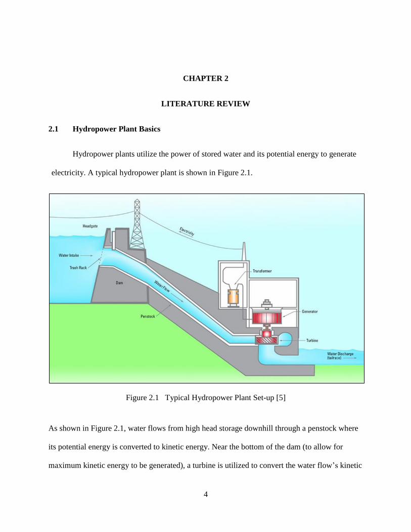
2.1 Hydropower Plant Basics
Hydropower plants utilize the power of stored water and its potential energy to generate
electricity. A typical hydropower plant is shown in Figure 2.1.
Figure 2.1 Typical Hydropower Plant Set-up [5]
As shown in Figure 2.1, water flows from high head storage downhill through a penstock where
its potential energy is converted to kinetic energy. Near the bottom of the dam (to allow for
maximum kinetic energy to be generated), a turbine is utilized to convert the water flow’s kinetic
5
energy into mechanical energy. The mechanical energy is transported via a rotating shaft to the
generator where it is then transformed into electrical energy. All electrical energy is then
transformed into high voltage current to be transported away from the dam and to energy
consumers via transmission wires.
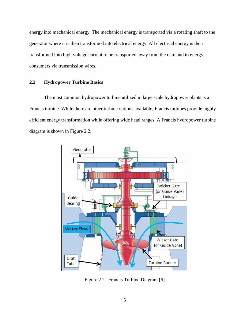
2.2 Hydropower Turbine Basics
The most common hydropower turbine utilized in large scale hydropower plants is a
Francis turbine. While there are other turbine options available, Francis turbines provide highly
efficient energy transformation while offering wide head ranges. A Francis hydropower turbine
diagram is shown in Figure 2.2.
Figure 2.2 Francis Turbine Diagram [6]
6
As shown in Figure 2.2, a Francis turbine generates power by allowing water with high
kinetic energy to pass through the turbine runner, spinning the shaft connected to the generator.
The water flow through the turbine and subsequently the power output of the turbine is
controlled via the wicket gates.
2.3 Cavitation Erosion
Cavitation is the formation of vapor cavities within a flow. The complex flows within a
hydropower turbine can experience local pressure drops that fall below the liquid's vapor
pressure, resulting in cavitation. The two main influences on the rate at which these vapor
structures form and collapse is determined by (1) the static pressure at the runner’s level and
(2) the superimposed dynamic pressure pulsation of the liquid's flow associated with the hydro
turbine's design, the active hydraulic conditions and operating point within the turbine.
Consequently, the vapor structures size and formation are statistically random by nature [7] [8].
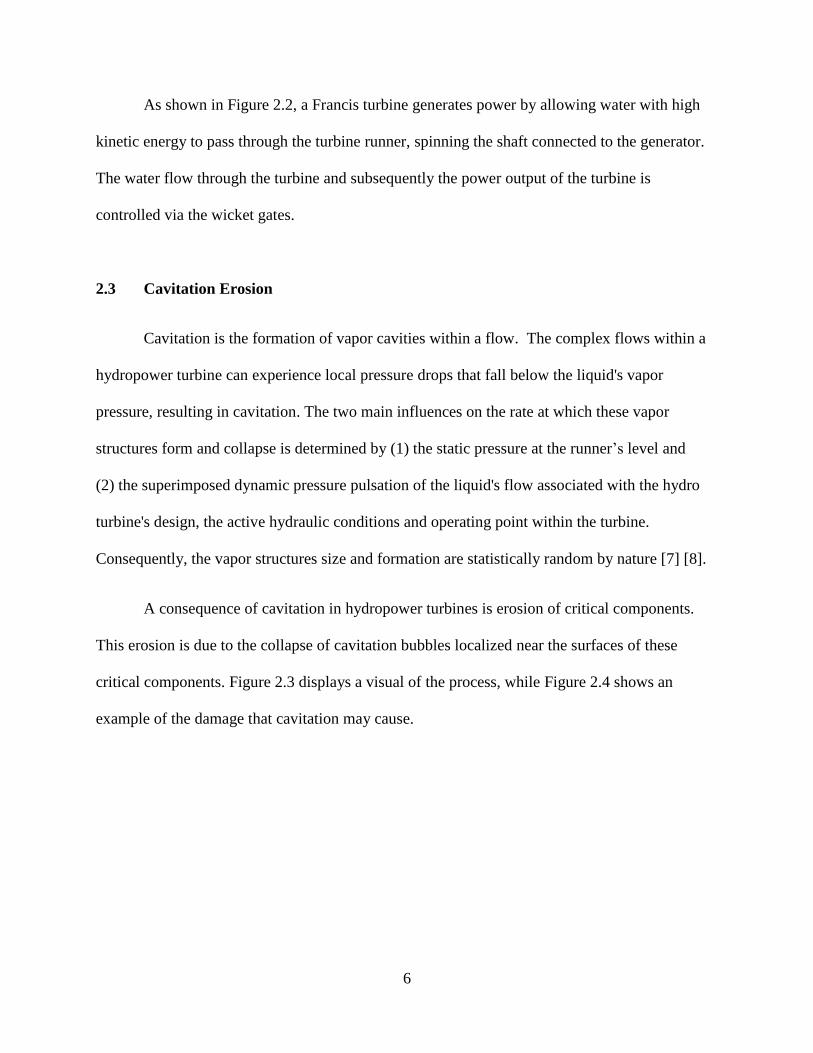
A consequence of cavitation in hydropower turbines is erosion of critical components.
This erosion is due to the collapse of cavitation bubbles localized near the surfaces of these
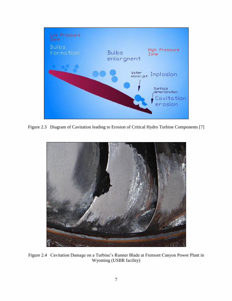
critical components. Figure 2.3 displays a visual of the process, while Figure 2.4 shows an
example of the damage that cavitation may cause.
7
Figure 2.3 Diagram of Cavitation leading to Erosion of Critical Hydro Turbine Components [7]
Figure 2.4 Cavitation Damage on a Turbine’s Runner Blade at Fremont Canyon Power Plant in
Wyoming (USBR facility)
8
As shown in Figure 2.3, cavitation bubbles move from a low-pressure zone to a high-
pressure zone, at which point they implode causing a water micro-jet. Harrison in 1952
determined theoretically that cavitation bubble implosion entails an infinite inward radial
velocity and thus an infinite pressure is developed local to the implosion site; it is practically
interpreted that cavitation implosion causes localized pressures in the gigapascal range [9]. It is
these localized impulses/micro-jets that lead to cavitation erosion areas where the vapor
structures ultimately collapse. The erosion rate can be related to the energy carried in the vapor
structures, their rate per unit time and the erosion resistance of the material.
When a new material is subjected to cavitation impacts, it first undergoes a plastic
deformation period where there is no material loss; this is referred to as the incubation period.
Over time, this plastic deformation turns to micro-cracks, which leads to loss of material. If
cavitation impacts are allowed to continue on a material for an extended amount of time, material
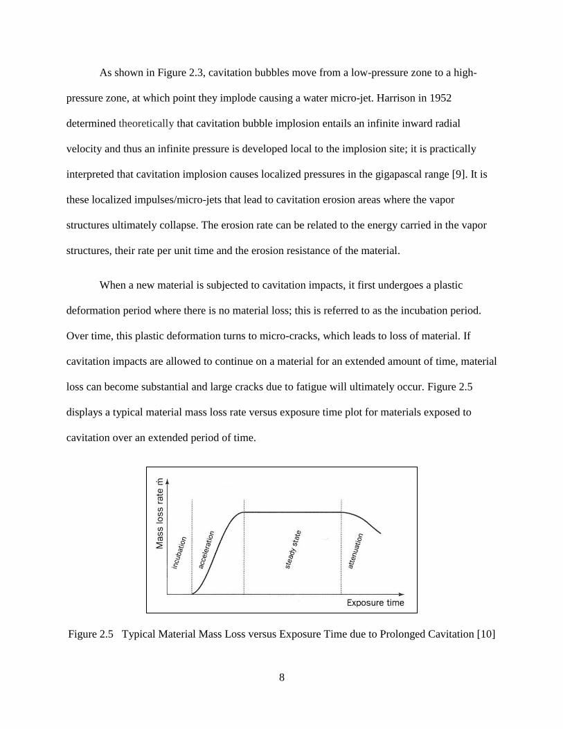
loss can become substantial and large cracks due to fatigue will ultimately occur. Figure 2.5
displays a typical material mass loss rate versus exposure time plot for materials exposed to
cavitation over an extended period of time.
Figure 2.5 Typical Material Mass Loss versus Exposure Time due to Prolonged Cavitation [10]
9
2.4 Previous Research
Over the past three decades, there has been research on cavitation erosion and the
development of cavitation detection for hydropower turbines. The major contributors include
Hydro-Quebec (HQ), Tennessee Valley Authority (TVA), Swiss Federal Institute of Technology
Lausanne (EPFL), Technical University of Catalonia (UPC), Korto Cavitation Services, and the
USBR. Most of the research has been focused on the determination of damaging cavitation on
hydropower turbine's runners. Turbine runners are the single most expensive component of a
hydro turbine and the most frequent cavitation damaged component.
The majority of cavitation monitoring is performed using either accelerometers or AE
sensors [11] [12]. The sensors are most commonly placed in one of three locations, namely
wicket gates linkages, guide bearings or the draft tube of the hydro turbine (See Figure 2.2 for
visual of locations) [13]. These three locations provide the most direct mechanical link from
cavitation impact locations to available sensor locations [14].
The simplest cavitation monitoring method involves computing the root mean square
amplitude (RMS) of the signal output from the instrumentation on the turbine and working to
correlate RMS output to cavitation aggressiveness. More in-depth analysis has also been carried
out; some examples of more involved analyses involve the following [15] [16] [17] [18] [19]
[20] [21] [22] [23]:
Identification from time traces of ‘bursts’ or peaks representative of the cavitation
erosion.
Amplitude demodulation of high frequency bands.
10
Utilizing the Hilbert transform to process the cavitation signal, resulting in an analytical
function from which harmonics are computed.
In addition, HQ, EPFL, and UPC have spearheaded two major advances in cavitation
monitoring. The first is the characterization of the transfer functions from cavitation impact
locations to the sensor locations. By using an instrumented impact hammer to impact a stationary
dewatered turbine runner while measuring at the determined sensor locations, the absolute
aggressiveness of the cavitation can be determined from the sensor outputs during in-field
monitoring. Determining the transfer function is referred is often referred to as calibration of the
cavitation detection system [21]. The transfer function is an amplitude ratio between the known
or anticipated cavitation impact locations and the sensor locations. By determining the amplitude
ratio, the Absolute Cavitation Aggressiveness, measured in Kg/10,000 Hrs can be
determined [7]. This technique has the inherent unknown that all transfer function measurements
are taken while the turbine is stationary and dewatered, thus leaving the question of how does the
fluid interaction effect the transfer functions during operation [24].
The second advancement in cavitation detection monitoring was published by EPFL and
UPC in 2003/2004 [24] [25]. They used accelerometers mounted directly to the rotating shaft of
a turbine to record cavitation signatures. The data was then transmitted wirelessly back the
acquisition system. Mounting the accelerometers directly to the shaft provides the most direct
mechanical link from the impact locations on the runner to the sensors. A case study will be
presented to demonstrate the advantages of rotating shaft mounted sensors versus stationary
sensor locations and present the reader with an example of cavitation detection methodology.
11
2.4.1 Example Case Study
The case study is titled: “Cavitation Erosion Prediction in Hydro Turbines from Onboard
Vibrations” and was completed by a team including engineers from EPFL and UPC [24]. The
case study includes the most current state of the art in cavitation detection, both wireless data
acquisition from a sensor located on the turbines shaft and transfer function determination used
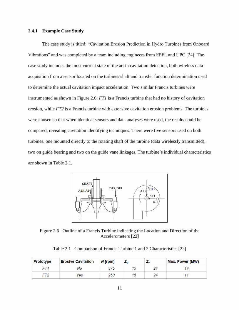
to determine the actual cavitation impact acceleration. Two similar Francis turbines were
instrumented as shown in Figure 2.6; FT1 is a Francis turbine that had no history of cavitation
erosion, while FT2 is a Francis turbine with extensive cavitation erosion problems. The turbines
were chosen so that when identical sensors and data analyses were used, the results could be
compared, revealing cavitation identifying techniques. There were five sensors used on both
turbines, one mounted directly to the rotating shaft of the turbine (data wirelessly transmitted),
two on guide bearing and two on the guide vane linkages. The turbine’s individual characteristics
are shown in Table 2.1.
Figure 2.6 Outline of a Francis Turbine indicating the Location and Direction of the
Accelerometers [22]
Table 2.1 Comparison of Francis Turbine 1 and 2 Characteristics [22]
12
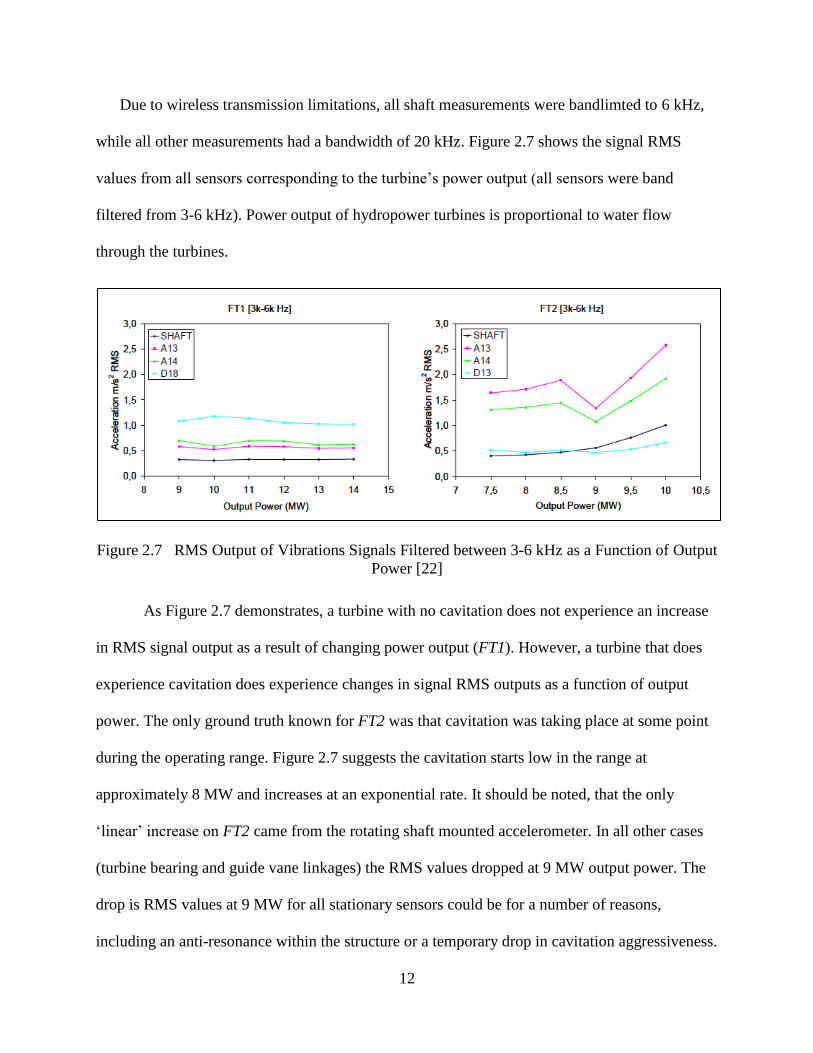
Due to wireless transmission limitations, all shaft measurements were bandlimted to 6 kHz,
while all other measurements had a bandwidth of 20 kHz. Figure 2.7 shows the signal RMS
values from all sensors corresponding to the turbine’s power output (all sensors were band
filtered from 3-6 kHz). Power output of hydropower turbines is proportional to water flow
through the turbines.
Figure 2.7 RMS Output of Vibrations Signals Filtered between 3-6 kHz as a Function of Output
Power [22]
As Figure 2.7 demonstrates, a turbine with no cavitation does not experience an increase
in RMS signal output as a result of changing power output (FT1). However, a turbine that does
experience cavitation does experience changes in signal RMS outputs as a function of output
power. The only ground truth known for FT2 was that cavitation was taking place at some point
during the operating range. Figure 2.7 suggests the cavitation starts low in the range at
approximately 8 MW and increases at an exponential rate. It should be noted, that the only
‘linear’ increase on FT2 came from the rotating shaft mounted accelerometer. In all other cases
(turbine bearing and guide vane linkages) the RMS values dropped at 9 MW output power. The
drop is RMS values at 9 MW for all stationary sensors could be for a number of reasons,
including an anti-resonance within the structure or a temporary drop in cavitation aggressiveness.
13
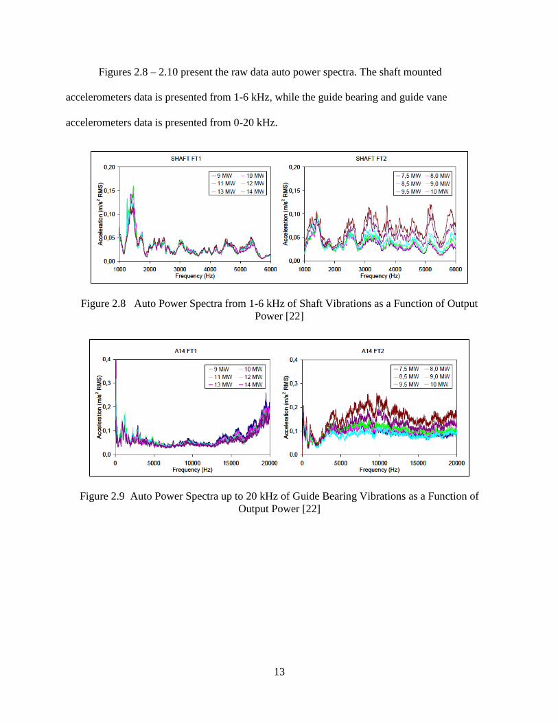
Figures 2.8 – 2.10 present the raw data auto power spectra. The shaft mounted
accelerometers data is presented from 1-6 kHz, while the guide bearing and guide vane
accelerometers data is presented from 0-20 kHz.
Figure 2.8 Auto Power Spectra from 1-6 kHz of Shaft Vibrations as a Function of Output
Power [22]
Figure 2.9 Auto Power Spectra up to 20 kHz of Guide Bearing Vibrations as a Function of
Output Power [22]
14
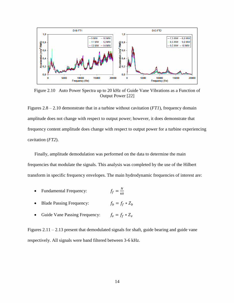
Figure 2.10 Auto Power Spectra up to 20 kHz of Guide Vane Vibrations as a Function of
Output Power [22]
Figures 2.8 – 2.10 demonstrate that in a turbine without cavitation (FT1), frequency domain
amplitude does not change with respect to output power; however, it does demonstrate that
frequency content amplitude does change with respect to output power for a turbine experiencing
cavitation (FT2).
Finally, amplitude demodulation was performed on the data to determine the main
frequencies that modulate the signals. This analysis was completed by the use of the Hilbert
transform in specific frequency envelopes. The main hydrodynamic frequencies of interest are:
Fundamental Frequency:
Blade Passing Frequency:
Guide Vane Passing Frequency:
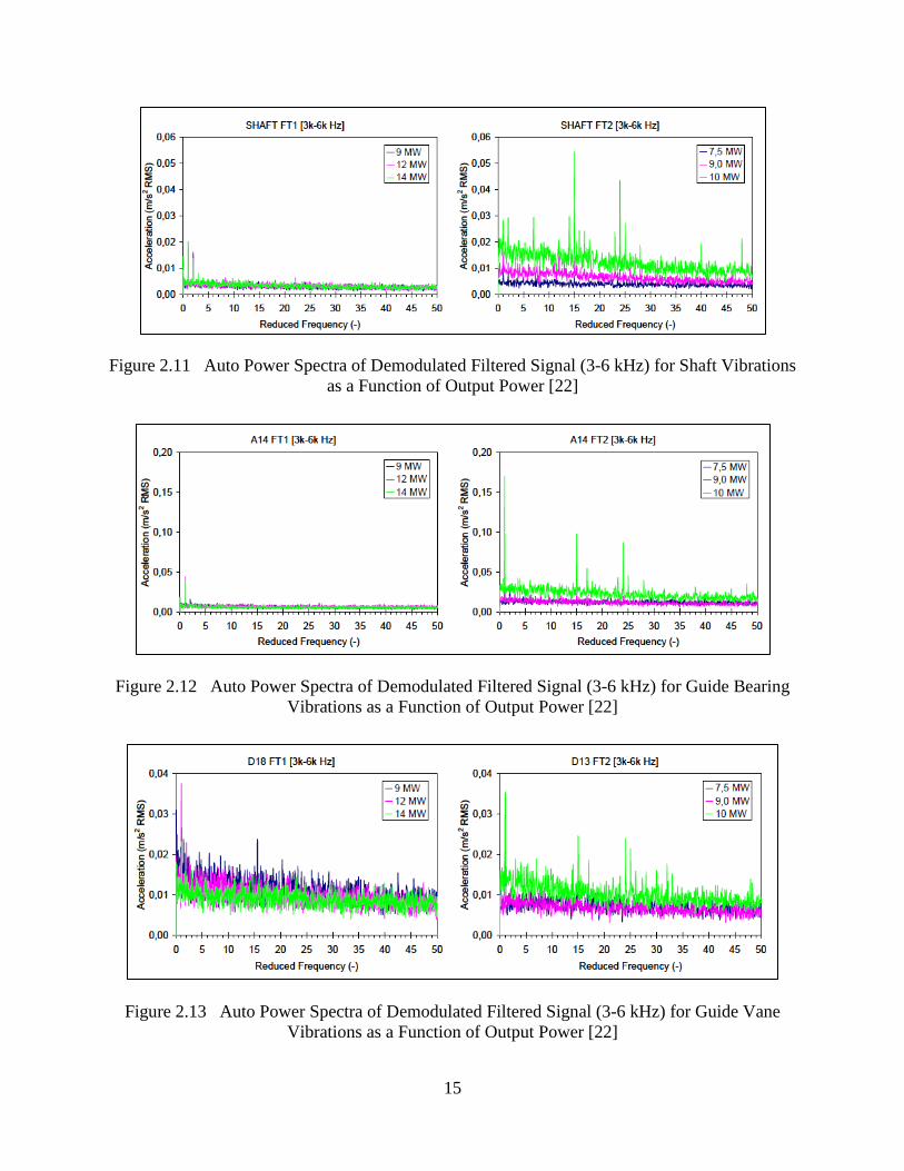
Figures 2.11 – 2.13 present that demodulated signals for shaft, guide bearing and guide vane
respectively. All signals were band filtered between 3-6 kHz.
15
Figure 2.11 Auto Power Spectra of Demodulated Filtered Signal (3-6 kHz) for Shaft Vibrations
as a Function of Output Power [22]
Figure 2.12 Auto Power Spectra of Demodulated Filtered Signal (3-6 kHz) for Guide Bearing
Vibrations as a Function of Output Power [22]
Figure 2.13 Auto Power Spectra of Demodulated Filtered Signal (3-6 kHz) for Guide Vane
Vibrations as a Function of Output Power [22]
16
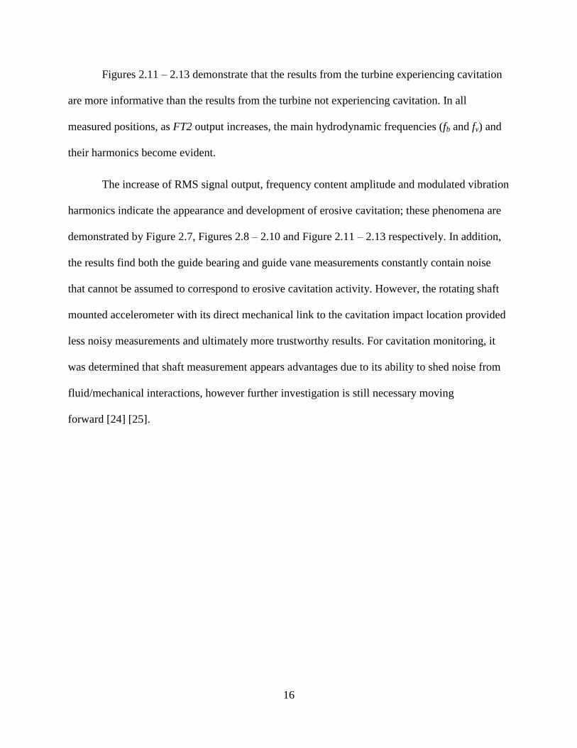
Figures 2.11 – 2.13 demonstrate that the results from the turbine experiencing cavitation
are more informative than the results from the turbine not experiencing cavitation. In all
measured positions, as FT2 output increases, the main hydrodynamic frequencies (fb and fv) and
their harmonics become evident.
The increase of RMS signal output, frequency content amplitude and modulated vibration
harmonics indicate the appearance and development of erosive cavitation; these phenomena are
demonstrated by Figure 2.7, Figures 2.8 – 2.10 and Figure 2.11 – 2.13 respectively. In addition,
the results find both the guide bearing and guide vane measurements constantly contain noise
that cannot be assumed to correspond to erosive cavitation activity. However, the rotating shaft
mounted accelerometer with its direct mechanical link to the cavitation impact location provided
less noisy measurements and ultimately more trustworthy results. For cavitation monitoring, it
was determined that shaft measurement appears advantages due to its ability to shed noise from
fluid/mechanical interactions, however further investigation is still necessary moving
forward [24] [25].

17
CHAPTER 3
FUNDAMENTAL RESEARCH QUESTIONS, GOALS AND PURPOSE
The goal of this research is to further develop and validate tools and methods for on-site
hydropower turbine cavitation characterization and detection. Before developing these tools and
methods however, one must first ask, what are the fundamental research questions that need to
be addressed?
3.1 Fundamental Research Questions
With the goal of designing and implementing a non-intrusive cavitation
characterization/detection monitoring system, the following fundamental research questions must
be addressed:
I. Can cavitation be characterized via repeatable and discernible inherent characteristics
that are capable of being measured/monitored?
o Is it advantageous to focus the analysis on the time domain over the frequency
domain? Or vice versa?
II. Can the ability to 'listen' for damage within a hydropower turbine be demonstrated from a
'known' input? i.e. Can a turbine with known cavitation history be characterized?
18
3.2 Project Objectives
At the start of this project there was optimism access to Hydropower Plants would be
possible between the Fall of 2012 and Spring of 2013 for onsite validation of methods
developed. Quickly however, it was determined that this was outside of the projects budget and
control. It was then determined that a simple cavitation inducing apparatus that could be
controlled in a laboratory environment would be developed and all non-intrusive cavitation
detection/characterization methods would be developed and validated on said apparatus. The
project objectives were determined to be:
I. Design, build and make operational a simple cavitation-inducing apparatus instrumented
to measure cavitation-induced vibration and acoustics.
II. The cavitation-induced vibroacoustical data will be analyzed to determine if there are
repeatable and discernible characteristics of cavitation that can be used for
characterization of the signal.
III. Develop metrics that clearly demonstrate volatility and cavitation onset within the flow.
19
CHAPTER 4
EXPERIMENTAL SET-UP
4.1 Design Conception
It was determined that a simple cavitation inducing apparatus would be designed and
built to be utilized in a laboratory environment for non-intrusive cavitation detection and
characterization. Working closely with a Senior Hydraulic Engineer of the USBR, it was
determined that the simplest and most controllable cavitation inducing set-up would be a
cavitation tunnel with an offset into the flow. The tunnel’s water flow would be fed by the USBR
Denver Federal Center Hydraulics’ Laboratory High Head Pump (HHP). The Hydraulics’
Laboratory HHP is comprised of a 250 hp variable speed drive motor and nine-stage pump. Two
pipes are available with the HHP set-up:
12” Diameter round piping
4” Square piping
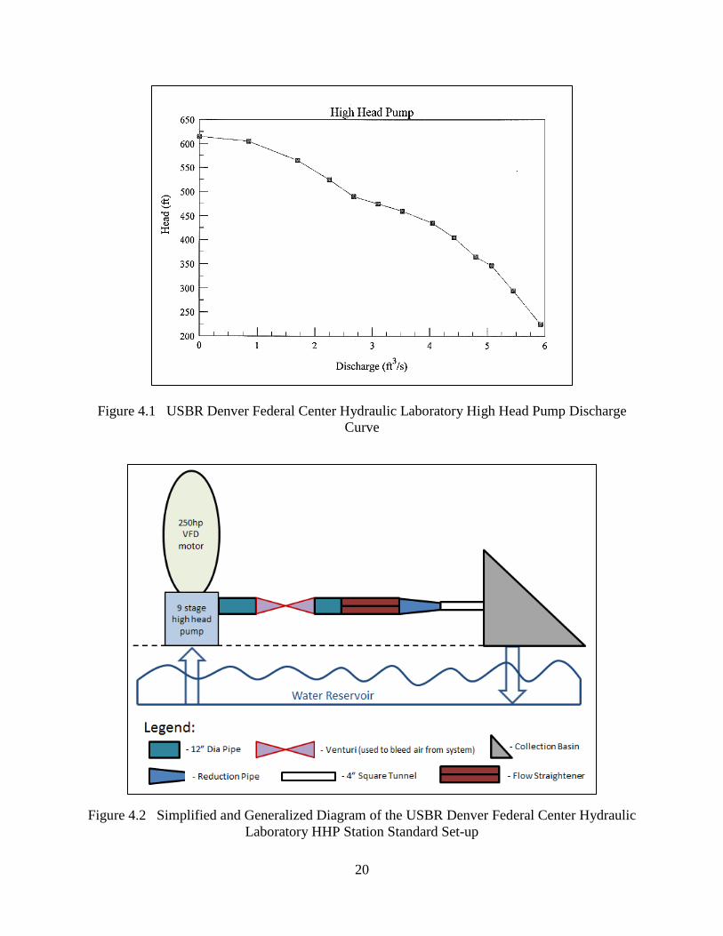
Figure 4.1 presents the HHP discharge curve while Figure 4.2 presents a simplified and
generalized diagram of the HHP station standard set-up. It was determined from the available
piping sizes, that a four inch square cavitation tunnel with an offset would be designed for
inducing and studying cavitation.
20
Figure 4.1 USBR Denver Federal Center Hydraulic Laboratory High Head Pump Discharge
Curve
Figure 4.2 Simplified and Generalized Diagram of the USBR Denver Federal Center Hydraulic
Laboratory HHP Station Standard Set-up
21
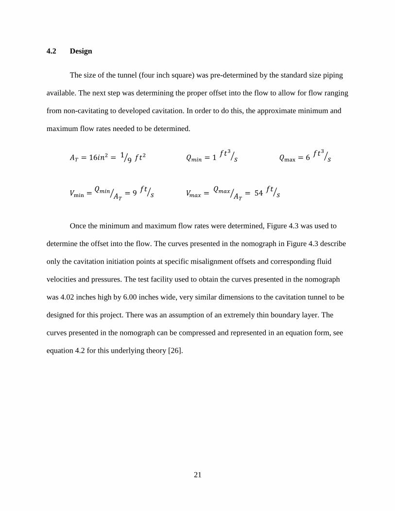
4.2 Design
The size of the tunnel (four inch square) was pre-determined by the standard size piping
available. The next step was determining the proper offset into the flow to allow for flow ranging
from non-cavitating to developed cavitation. In order to do this, the approximate minimum and
maximum flow rates needed to be determined.
⁄
⁄
⁄
⁄
⁄
⁄
⁄
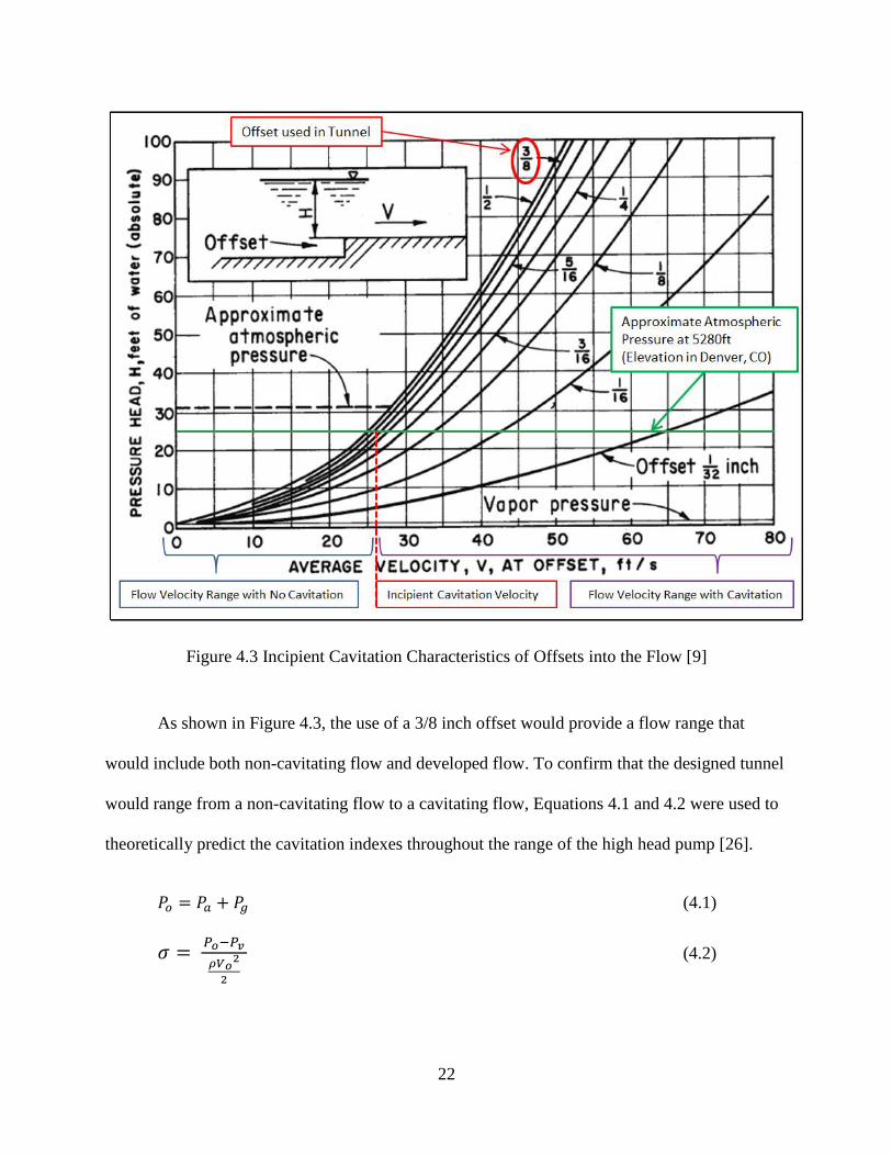
Once the minimum and maximum flow rates were determined, Figure 4.3 was used to
determine the offset into the flow. The curves presented in the nomograph in Figure 4.3 describe
only the cavitation initiation points at specific misalignment offsets and corresponding fluid
velocities and pressures. The test facility used to obtain the curves presented in the nomograph
was 4.02 inches high by 6.00 inches wide, very similar dimensions to the cavitation tunnel to be
designed for this project. There was an assumption of an extremely thin boundary layer. The
curves presented in the nomograph can be compressed and represented in an equation form, see
equation 4.2 for this underlying theory [26].
22
Figure 4.3 Incipient Cavitation Characteristics of Offsets into the Flow [9]
As shown in Figure 4.3, the use of a 3/8 inch offset would provide a flow range that
would include both non-cavitating flow and developed flow. To confirm that the designed tunnel
would range from a non-cavitating flow to a cavitating flow, Equations 4.1 and 4.2 were used to
theoretically predict the cavitation indexes throughout the range of the high head pump [26].
(4.1)
(4.2)
23
Where:
σ: Cavitation Index
Po: Reference pressure – Pressure in free stream flow at offset
Pa: Atmospheric pressure
Pg: Gage pressure
: Density
Vo: Average fluid velocity in free stream flow at offset
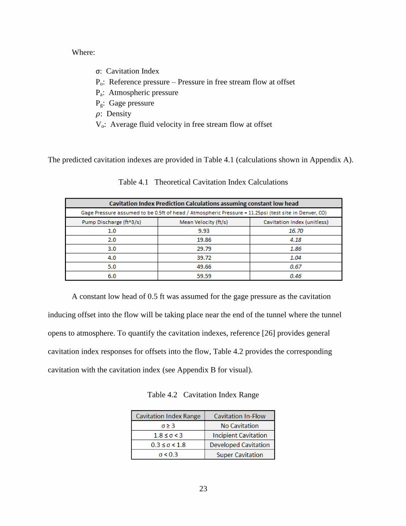
The predicted cavitation indexes are provided in Table 4.1 (calculations shown in Appendix A).
Table 4.1 Theoretical Cavitation Index Calculations
A constant low head of 0.5 ft was assumed for the gage pressure as the cavitation
inducing offset into the flow will be taking place near the end of the tunnel where the tunnel
opens to atmosphere. To quantify the cavitation indexes, reference [26] provides general
cavitation index responses for offsets into the flow, Table 4.2 provides the corresponding
cavitation with the cavitation index (see Appendix B for visual).
Table 4.2 Cavitation Index Range
24
Table 4.2 presents four separate cavitation states. No cavitation describes a flow devoid
of vapor cavities. Incipient cavitation describes a flow with intermittent small vapor cavities, a
flow where cavitation is starting. Developed cavitation describes a flow with many individual
bubbles, constantly forming from the cavitation inducing offset. To the naked eye, developed
cavitation appears to be a fuzzy white cloud within a flow. Super cavitation describes a flow
where the cloud suddenly forms larger bubbles or supercavitating pockets and the
bubbles/pockets move downstream a substantial distance further then during developed
cavitation.
As Table 4.1 shows, given the available pump discharge, flows ranging from non-
cavitating to near super cavitation will be achievable. While it was desired for the minimum flow
rates to be laminar, there were expectations that even the minimum flows would be turbulent
given the high velocities and small tunnel (turbulence does not imply cavitation). To check for
turbulence, the Reynolds Number (Re) was determined for each flow rate. Re is a dimensionless
number which provides the ratio of the inertial forces to the viscous forces. Low Re represent
laminar flow, flow in which viscous forces are dominant, these fluid processes are generally
smooth or quiet flows (Re < 2300). High Re represent flows dominated by inertial forces, these
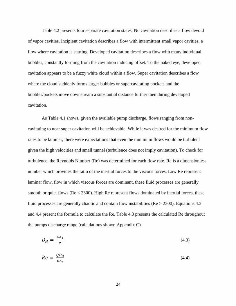
fluid processes are generally chaotic and contain flow instabilities (Re > 2300). Equations 4.3
and 4.4 present the formula to calculate the Re, Table 4.3 presents the calculated Re throughout
the pumps discharge range (calculations shown Appendix C).
(4.3)
(4.4)
25
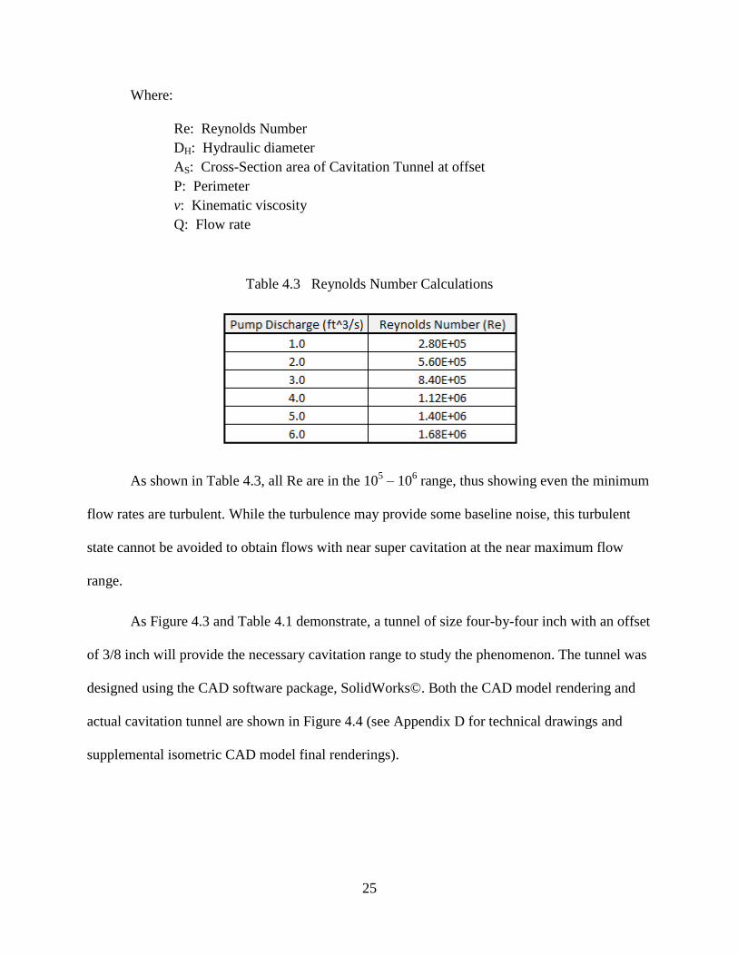
Where:
Re: Reynolds Number
DH: Hydraulic diameter
AS: Cross-Section area of Cavitation Tunnel at offset
P: Perimeter
v: Kinematic viscosity
Q: Flow rate
Table 4.3 Reynolds Number Calculations
As shown in Table 4.3, all Re are in the 105 – 10
6 range, thus showing even the minimum
flow rates are turbulent. While the turbulence may provide some baseline noise, this turbulent
state cannot be avoided to obtain flows with near super cavitation at the near maximum flow
range.
As Figure 4.3 and Table 4.1 demonstrate, a tunnel of size four-by-four inch with an offset
of 3/8 inch will provide the necessary cavitation range to study the phenomenon. The tunnel was
designed using the CAD software package, SolidWorks©. Both the CAD model rendering and
actual cavitation tunnel are shown in Figure 4.4 (see Appendix D for technical drawings and
supplemental isometric CAD model final renderings).
26
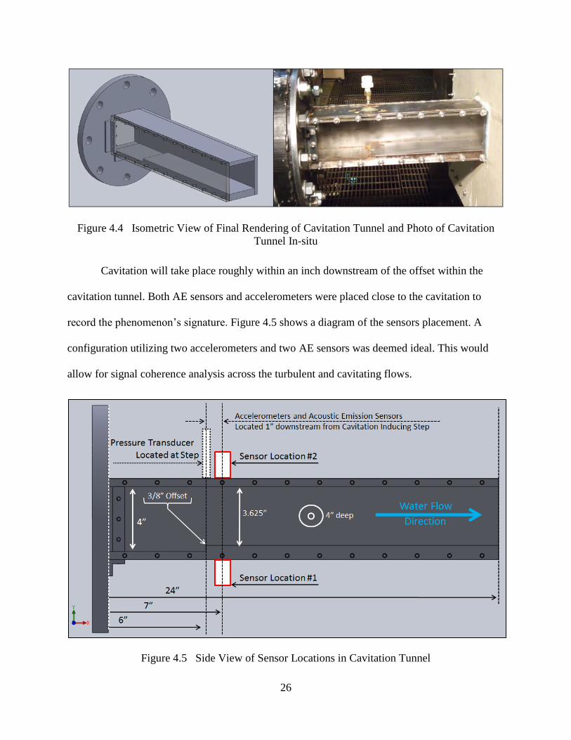
Figure 4.4 Isometric View of Final Rendering of Cavitation Tunnel and Photo of Cavitation
Tunnel In-situ
Cavitation will take place roughly within an inch downstream of the offset within the
cavitation tunnel. Both AE sensors and accelerometers were placed close to the cavitation to
record the phenomenon’s signature. Figure 4.5 shows a diagram of the sensors placement. A
configuration utilizing two accelerometers and two AE sensors was deemed ideal. This would
allow for signal coherence analysis across the turbulent and cavitating flows.
Figure 4.5 Side View of Sensor Locations in Cavitation Tunnel
27
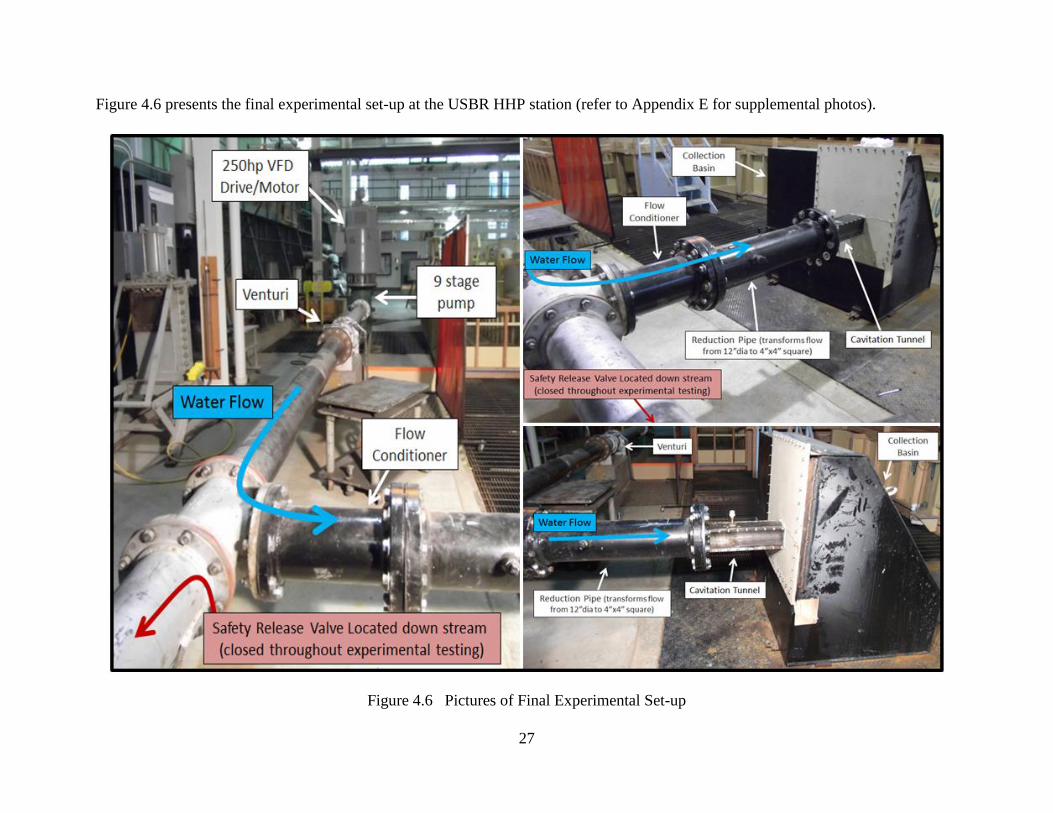
Figure 4.6 presents the final experimental set-up at the USBR HHP station (refer to Appendix E for supplemental photos).
Figure 4.6 Pictures of Final Experimental Set-up
28
CHAPTER 5
INSTRUMENTATION AND DATA ANALYSIS METHODS
5.1 Sensors
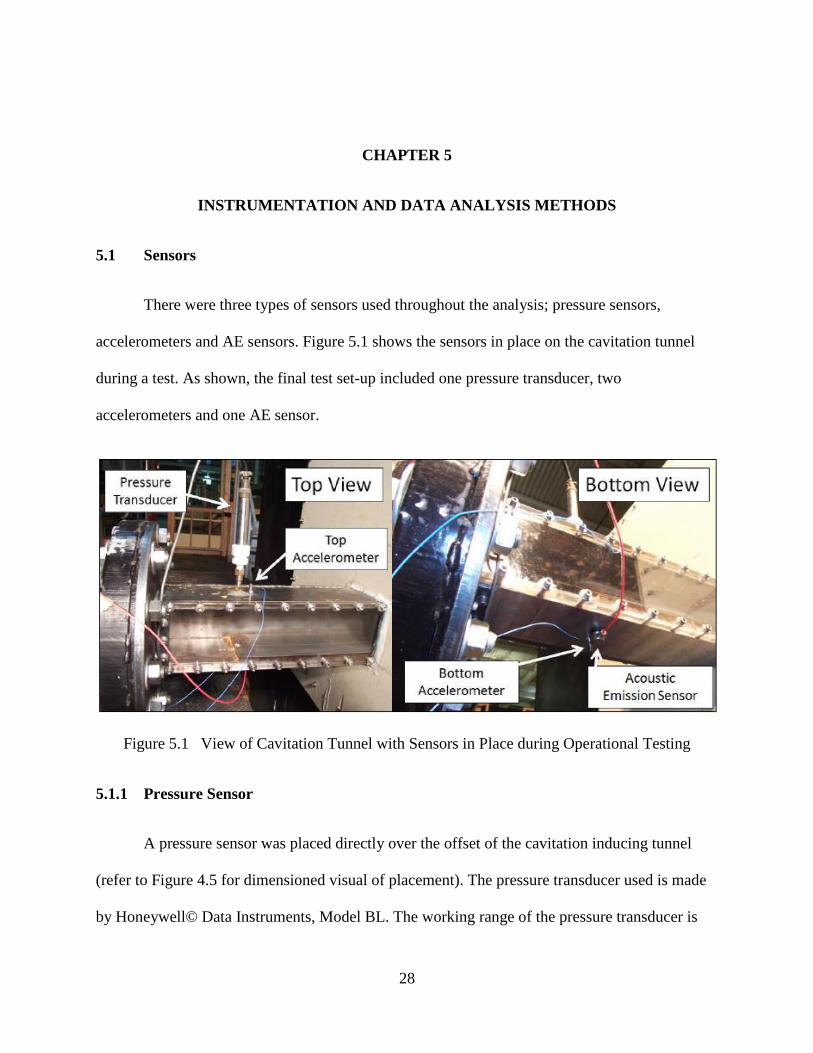
There were three types of sensors used throughout the analysis; pressure sensors,
accelerometers and AE sensors. Figure 5.1 shows the sensors in place on the cavitation tunnel
during a test. As shown, the final test set-up included one pressure transducer, two
accelerometers and one AE sensor.
Figure 5.1 View of Cavitation Tunnel with Sensors in Place during Operational Testing
5.1.1 Pressure Sensor
A pressure sensor was placed directly over the offset of the cavitation inducing tunnel
(refer to Figure 4.5 for dimensioned visual of placement). The pressure transducer used is made
by Honeywell© Data Instruments, Model BL. The working range of the pressure transducer is
29
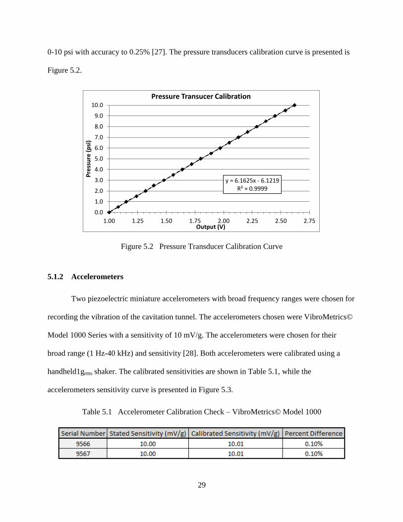
0-10 psi with accuracy to 0.25% [27]. The pressure transducers calibration curve is presented is
Figure 5.2.
Figure 5.2 Pressure Transducer Calibration Curve
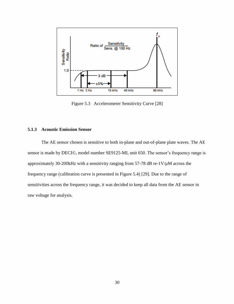
5.1.2 Accelerometers
Two piezoelectric miniature accelerometers with broad frequency ranges were chosen for
recording the vibration of the cavitation tunnel. The accelerometers chosen were VibroMetrics©
Model 1000 Series with a sensitivity of 10 mV/g. The accelerometers were chosen for their
broad range (1 Hz-40 kHz) and sensitivity [28]. Both accelerometers were calibrated using a
handheld1grms shaker. The calibrated sensitivities are shown in Table 5.1, while the
accelerometers sensitivity curve is presented in Figure 5.3.
Table 5.1 Accelerometer Calibration Check – VibroMetrics© Model 1000
y = 6.1625x - 6.1219 R² = 0.9999
0.0
1.0
2.0
3.0
4.0
5.0
6.0
7.0
8.0
9.0
10.0
1.00 1.25 1.50 1.75 2.00 2.25 2.50 2.75
Pre
ssu
re (
psi
)
Output (V)
Pressure Transucer Calibration
30
Figure 5.3 Accelerometer Sensitivity Curve [28]
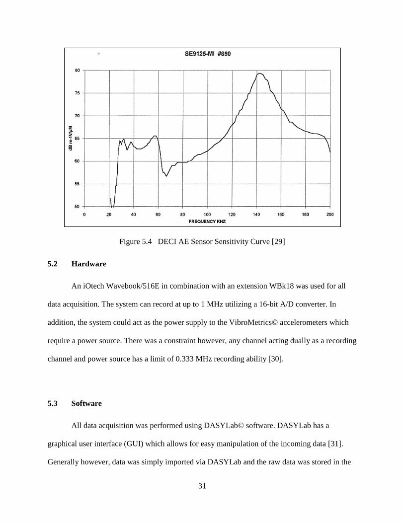
5.1.3 Acoustic Emission Sensor
The AE sensor chosen is sensitive to both in-plane and out-of-plane plate waves. The AE
sensor is made by DECI©, model number SE9125-MI, unit 650. The sensor’s frequency range is
approximately 30-200kHz with a sensitivity ranging from 57-78 dB re-1V/µM across the
frequency range (calibration curve is presented in Figure 5.4) [29]. Due to the range of
sensitivities across the frequency range, it was decided to keep all data from the AE sensor in
raw voltage for analysis.
31
Figure 5.4 DECI AE Sensor Sensitivity Curve [29]
5.2 Hardware
An iOtech Wavebook/516E in combination with an extension WBk18 was used for all
data acquisition. The system can record at up to 1 MHz utilizing a 16-bit A/D converter. In
addition, the system could act as the power supply to the VibroMetrics© accelerometers which
require a power source. There was a constraint however, any channel acting dually as a recording
channel and power source has a limit of 0.333 MHz recording ability [30].
5.3 Software
All data acquisition was performed using DASYLab© software. DASYLab has a
graphical user interface (GUI) which allows for easy manipulation of the incoming data [31].
Generally however, data was simply imported via DASYLab and the raw data was stored in the
32
American Standard Code for Information Exchange (ASCII). ASCII is a common format used to
exchange information between different software.
5.4 Data Acquisition Parameters
All testing and data acquisition was performed by using the following parameters:
Pressure transducer recorded at 1 kHz and RMS of signal calculated over one
second interval and recorded.
Accelerometers recorded simultaneously at 333 kHz for 14 seconds.
AE sensor recorded at 1 MHz for 9 seconds.
Samples rates and recording length were chosen based on sampling high enough to prevent
aliasing while keeping the ASCII files to a manageable size. Typical file sizes were on the order
of 102 megabytes.
5.5 Band-Pass Filtering
The first step in post-processing was to apply appropriate band-pass filters to the
accelerometer and acoustic emission data. The high pass filters will efficiently remove any DC
bias and low frequency noise which falls below the sensors effective sensing range. The low pass
filters will remove high frequency noise from the recorded data between the sensor’s effective
range limit and Nyquist frequency. Table 5.2 presents the filters used throughout the signal
processing.
Table 5.2 Butterworth Band Pass Filter Parameters Applied to All Data Prior to Post-Processing
33
All filters were designed to keep data taken within the sensors frequency range to be
reduced to a maximum of 0.998 magnitude. Also, any energy located at the Nyquist frequency
(Accelerometers: 167 kHz & AE Sensor: 500 kHz), was reduced to -75 dB and -40 dB
respectively. See Appendix F for confirming calculations. It is important to note that the ideal
high pass filter for the accelerometer data was not a two pole Butterworth with a cut-off
frequency equal to 1 Hz. However, the ideal high pass filter for the accelerometer data could not
be implemented due to resolution restrictions within the frequency domain. Due to this, the high
pass filter shown in Table 5.2 was implemented.
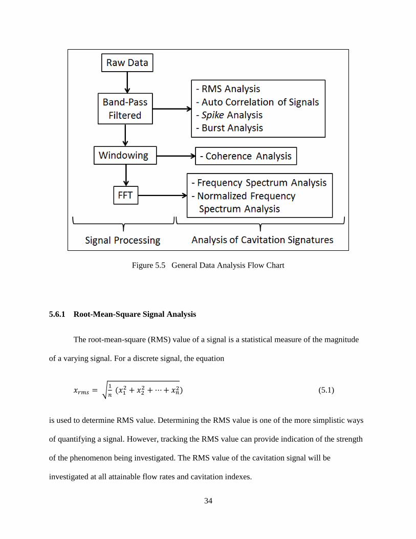
5.6 Data Analysis Background
There were many different analysis methods and metrics applied to the cavitation
monitoring data. Section 5.6 will explain the theoretical background and how the analysis
methods may be able to be used to characterize the cavitation signals. Chapter 6 will present the
results and characterization of the cavitation using the methods and metrics outlined. The general
data analysis flow is presented in Figure 5.5.
34
Figure 5.5 General Data Analysis Flow Chart
5.6.1 Root-Mean-Square Signal Analysis
The root-mean-square (RMS) value of a signal is a statistical measure of the magnitude
of a varying signal. For a discrete signal, the equation
√
(5.1)
is used to determine RMS value. Determining the RMS value is one of the more simplistic ways
of quantifying a signal. However, tracking the RMS value can provide indication of the strength
of the phenomenon being investigated. The RMS value of the cavitation signal will be
investigated at all attainable flow rates and cavitation indexes.
35
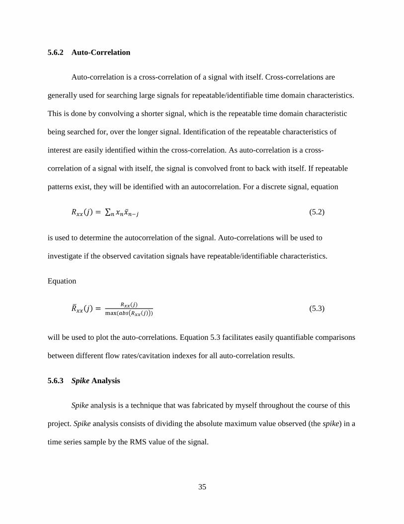
5.6.2 Auto-Correlation
Auto-correlation is a cross-correlation of a signal with itself. Cross-correlations are
generally used for searching large signals for repeatable/identifiable time domain characteristics.
This is done by convolving a shorter signal, which is the repeatable time domain characteristic
being searched for, over the longer signal. Identification of the repeatable characteristics of
interest are easily identified within the cross-correlation. As auto-correlation is a cross-
correlation of a signal with itself, the signal is convolved front to back with itself. If repeatable
patterns exist, they will be identified with an autocorrelation. For a discrete signal, equation
∑ (5.2)
is used to determine the autocorrelation of the signal. Auto-correlations will be used to
investigate if the observed cavitation signals have repeatable/identifiable characteristics.
Equation
( ) (5.3)
will be used to plot the auto-correlations. Equation 5.3 facilitates easily quantifiable comparisons
between different flow rates/cavitation indexes for all auto-correlation results.
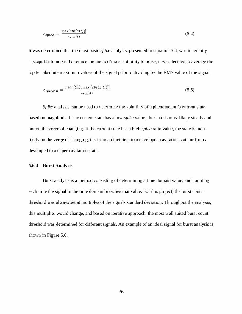
5.6.3 Spike Analysis
Spike analysis is a technique that was fabricated by myself throughout the course of this
project. Spike analysis consists of dividing the absolute maximum value observed (the spike) in a
time series sample by the RMS value of the signal.
36
{ ( )}
(5.4)
It was determined that the most basic spike analysis, presented in equation 5.4, was inherently
susceptible to noise. To reduce the method’s susceptibility to noise, it was decided to average the
top ten absolute maximum values of the signal prior to dividing by the RMS value of the signal.
[∑ { ( )}
]
(5.5)
Spike analysis can be used to determine the volatility of a phenomenon’s current state
based on magnitude. If the current state has a low spike value, the state is most likely steady and
not on the verge of changing. If the current state has a high spike ratio value, the state is most
likely on the verge of changing, i.e. from an incipient to a developed cavitation state or from a
developed to a super cavitation state.
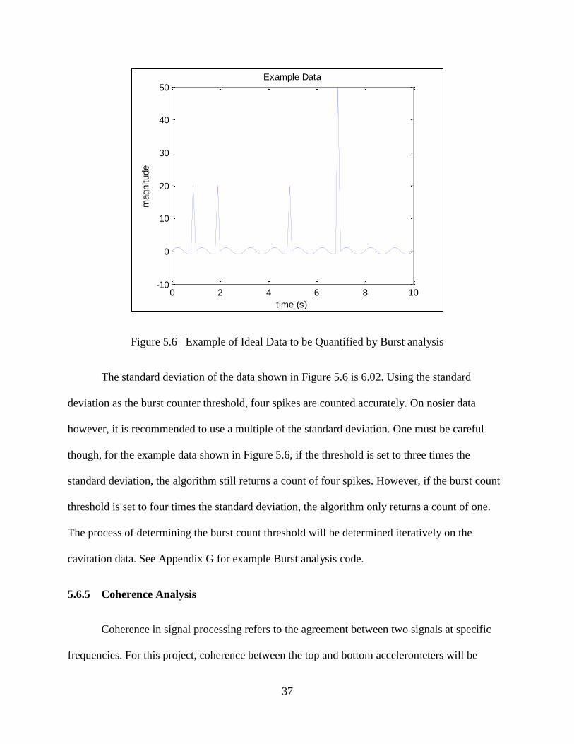
5.6.4 Burst Analysis
Burst analysis is a method consisting of determining a time domain value, and counting
each time the signal in the time domain breaches that value. For this project, the burst count
threshold was always set at multiples of the signals standard deviation. Throughout the analysis,
this multiplier would change, and based on iterative approach, the most well suited burst count
threshold was determined for different signals. An example of an ideal signal for burst analysis is
shown in Figure 5.6.
37
Figure 5.6 Example of Ideal Data to be Quantified by Burst analysis
The standard deviation of the data shown in Figure 5.6 is 6.02. Using the standard
deviation as the burst counter threshold, four spikes are counted accurately. On nosier data
however, it is recommended to use a multiple of the standard deviation. One must be careful
though, for the example data shown in Figure 5.6, if the threshold is set to three times the
standard deviation, the algorithm still returns a count of four spikes. However, if the burst count
threshold is set to four times the standard deviation, the algorithm only returns a count of one.
The process of determining the burst count threshold will be determined iteratively on the
cavitation data. See Appendix G for example Burst analysis code.
5.6.5 Coherence Analysis
Coherence in signal processing refers to the agreement between two signals at specific
frequencies. For this project, coherence between the top and bottom accelerometers will be
0 2 4 6 8 10-10
0
10
20
30
40
50
time (s)
magnitude
Example Data
38
analyzed. Coherence between two real-valued signals, x(t) and y(t), is determined from
equation 5.6.
| |
(5.6)
Where:
Cxy: Coherence between two real-valued signals
Gxy: Cross spectral density of two real valued signals
Gxx: Auto-spectral density of x
Gyy: Auto-spectral density of y
The use of a Hanning window greatly reduces noise and allows for easier observation of
important characteristics revealed from the coherence. Coherence between the top and bottom
accelerometers could reveal natural frequencies of the system, common frequencies generated
from impacts and/or turbulent flow effects within the cavitation tunnel.
5.6.6 Frequency Spectrum Analysis
The use of the Fast Fourier Transform (FFT) is well known and a common analysis
technique used in signal processing. All data will be windowed and transformed into the
frequency domain utilizing the FFT and searched for prominent frequencies and frequency
bands. Figure 5.7 shows the basic technique demonstrated through a visual example.
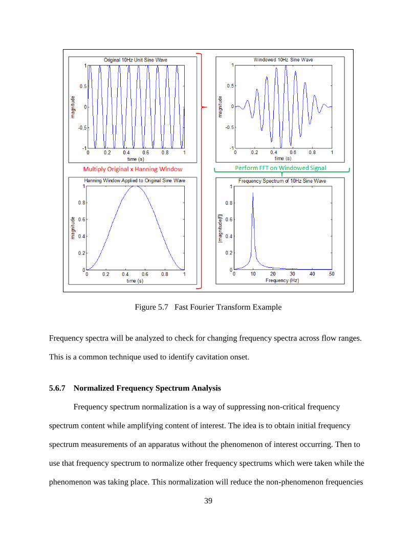
39
Figure 5.7 Fast Fourier Transform Example
Frequency spectra will be analyzed to check for changing frequency spectra across flow ranges.
This is a common technique used to identify cavitation onset.
5.6.7 Normalized Frequency Spectrum Analysis
Frequency spectrum normalization is a way of suppressing non-critical frequency
spectrum content while amplifying content of interest. The idea is to obtain initial frequency
spectrum measurements of an apparatus without the phenomenon of interest occurring. Then to
use that frequency spectrum to normalize other frequency spectrums which were taken while the
phenomenon was taking place. This normalization will reduce the non-phenomenon frequencies
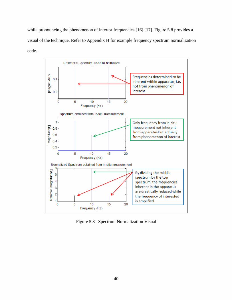
40
while pronouncing the phenomenon of interest frequencies [16] [17]. Figure 5.8 provides a
visual of the technique. Refer to Appendix H for example frequency spectrum normalization
code.
Figure 5.8 Spectrum Normalization Visual
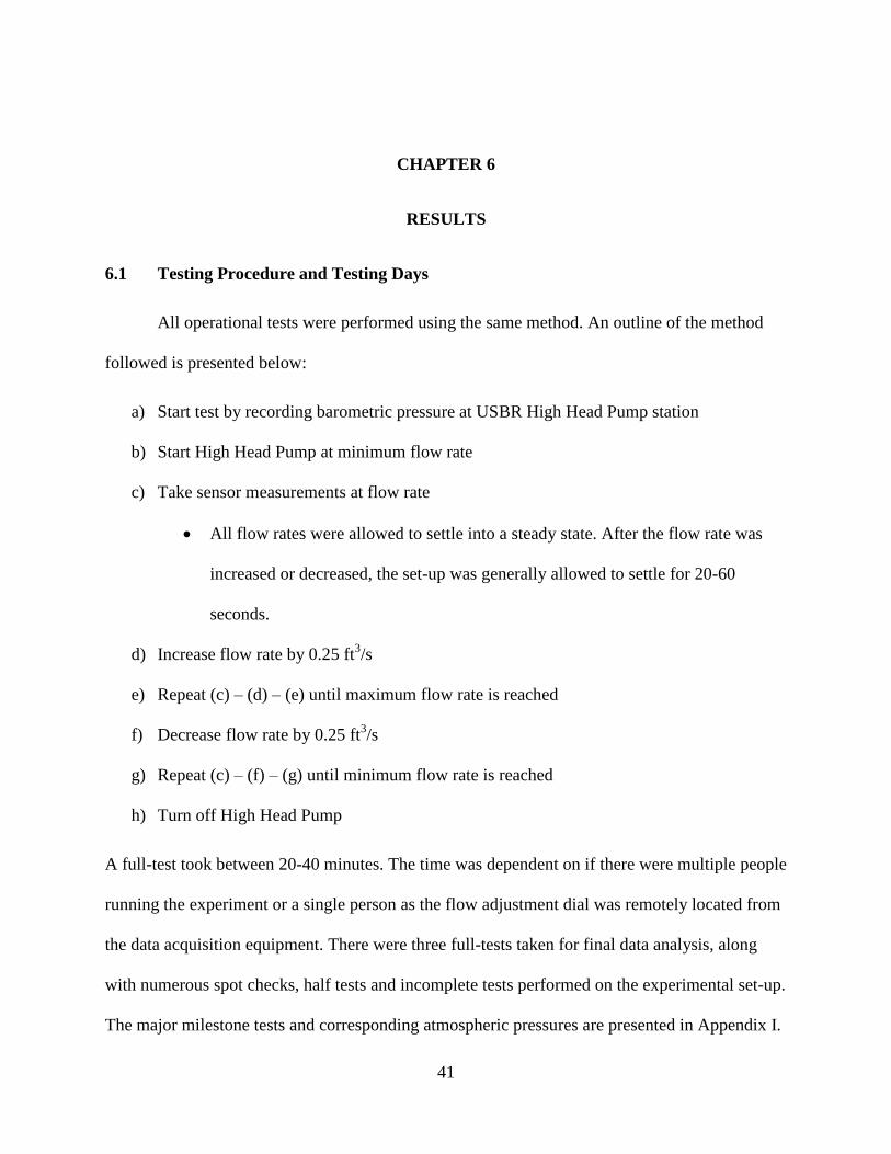
41
CHAPTER 6
RESULTS
6.1 Testing Procedure and Testing Days
All operational tests were performed using the same method. An outline of the method
followed is presented below:
a) Start test by recording barometric pressure at USBR High Head Pump station
b) Start High Head Pump at minimum flow rate
c) Take sensor measurements at flow rate
All flow rates were allowed to settle into a steady state. After the flow rate was
increased or decreased, the set-up was generally allowed to settle for 20-60
seconds.
d) Increase flow rate by 0.25 ft3/s
e) Repeat (c) – (d) – (e) until maximum flow rate is reached
f) Decrease flow rate by 0.25 ft3/s
g) Repeat (c) – (f) – (g) until minimum flow rate is reached
h) Turn off High Head Pump
A full-test took between 20-40 minutes. The time was dependent on if there were multiple people
running the experiment or a single person as the flow adjustment dial was remotely located from
the data acquisition equipment. There were three full-tests taken for final data analysis, along
with numerous spot checks, half tests and incomplete tests performed on the experimental set-up.
The major milestone tests and corresponding atmospheric pressures are presented in Appendix I.
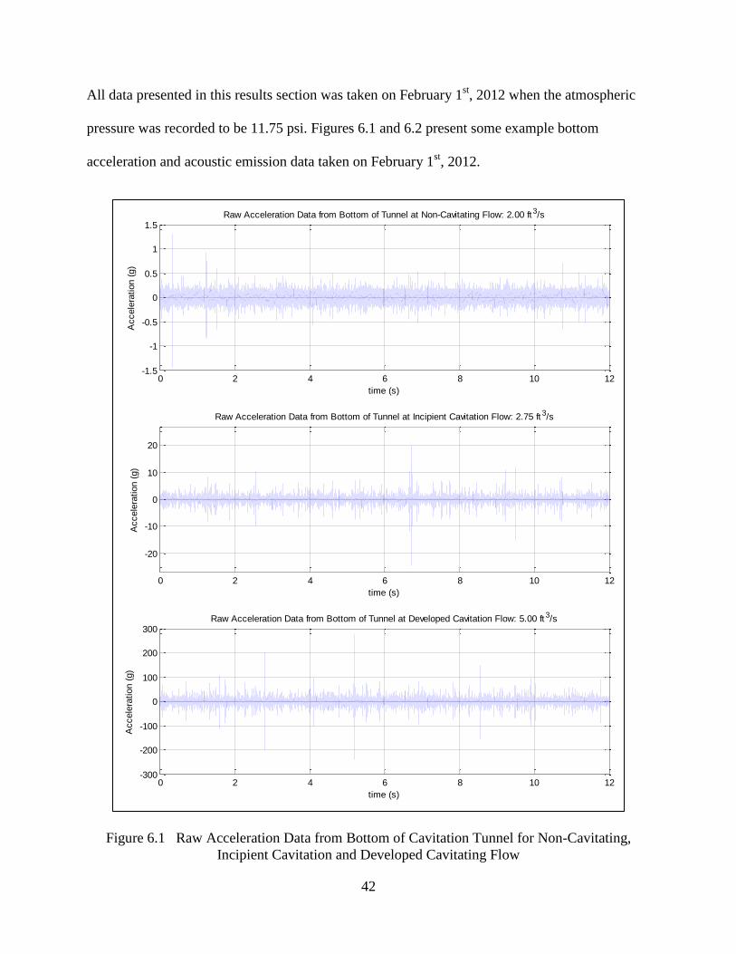
42
All data presented in this results section was taken on February 1st, 2012 when the atmospheric
pressure was recorded to be 11.75 psi. Figures 6.1 and 6.2 present some example bottom
acceleration and acoustic emission data taken on February 1st, 2012.
Figure 6.1 Raw Acceleration Data from Bottom of Cavitation Tunnel for Non-Cavitating,
Incipient Cavitation and Developed Cavitating Flow
0 2 4 6 8 10 12-1.5
-1
-0.5
0
0.5
1
1.5
time (s)
Accele
ration (
g)
Raw Acceleration Data from Bottom of Tunnel at Non-Cavitating Flow: 2.00 ft3/s
0 2 4 6 8 10 12
-20
-10
0
10
20
time (s)
Accele
ration (
g)
Raw Acceleration Data from Bottom of Tunnel at Incipient Cavitation Flow: 2.75 ft 3/s
0 2 4 6 8 10 12-300
-200
-100
0
100
200
300
time (s)
Accele
ration (
g)
Raw Acceleration Data from Bottom of Tunnel at Developed Cavitation Flow: 5.00 ft3/s
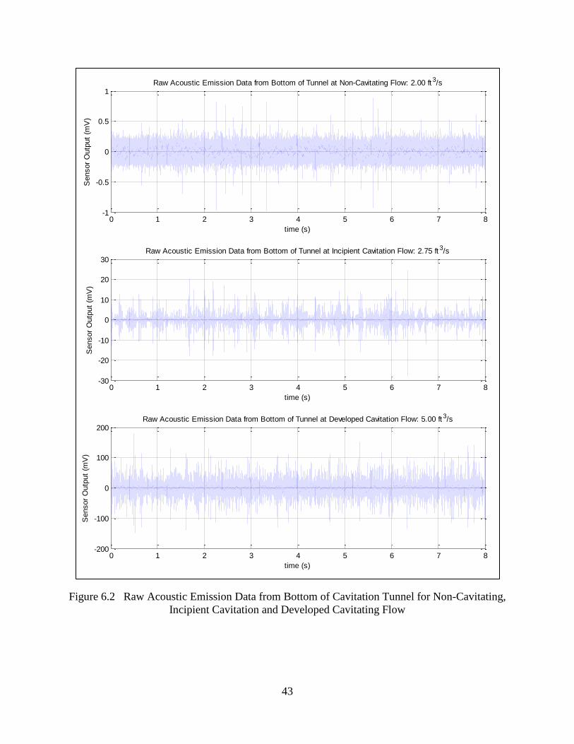
43
Figure 6.2 Raw Acoustic Emission Data from Bottom of Cavitation Tunnel for Non-Cavitating,
Incipient Cavitation and Developed Cavitating Flow
0 1 2 3 4 5 6 7 8-1
-0.5
0
0.5
1
time (s)
Sensor
Outp
ut
(mV
)Raw Acoustic Emission Data from Bottom of Tunnel at Non-Cavitating Flow: 2.00 ft 3/s
0 1 2 3 4 5 6 7 8-30
-20
-10
0
10
20
30
time (s)
Sensor
Outp
ut
(mV
)
Raw Acoustic Emission Data from Bottom of Tunnel at Incipient Cavitation Flow: 2.75 ft 3/s
0 1 2 3 4 5 6 7 8-200
-100
0
100
200
time (s)
Sensor
Outp
ut
(mV
)
Raw Acoustic Emission Data from Bottom of Tunnel at Developed Cavitation Flow: 5.00 ft 3/s
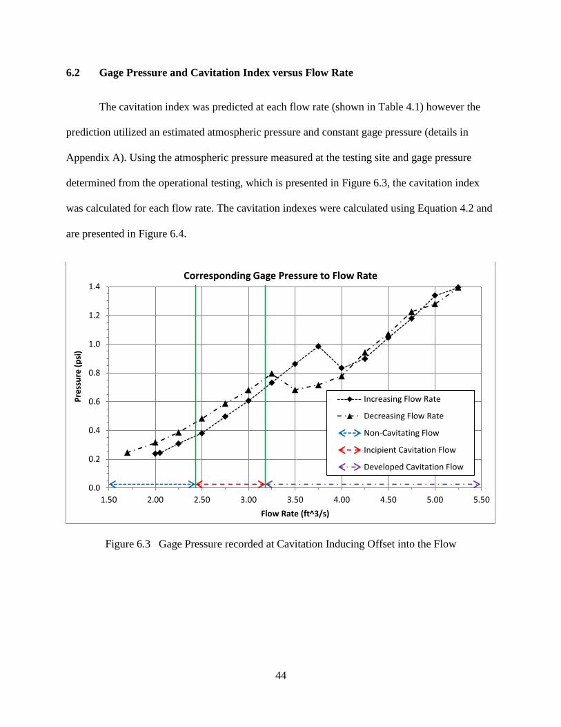
44
6.2 Gage Pressure and Cavitation Index versus Flow Rate
The cavitation index was predicted at each flow rate (shown in Table 4.1) however the
prediction utilized an estimated atmospheric pressure and constant gage pressure (details in
Appendix A). Using the atmospheric pressure measured at the testing site and gage pressure
determined from the operational testing, which is presented in Figure 6.3, the cavitation index
was calculated for each flow rate. The cavitation indexes were calculated using Equation 4.2 and
are presented in Figure 6.4.
Figure 6.3 Gage Pressure recorded at Cavitation Inducing Offset into the Flow
0.0
0.2
0.4
0.6
0.8
1.0
1.2
1.4
1.50 2.00 2.50 3.00 3.50 4.00 4.50 5.00 5.50
Pre
ssu
re (
psi
)
Flow Rate (ft^3/s)
Corresponding Gage Pressure to Flow Rate
Increasing Flow Rate
Decreasing Flow Rate
Non-Cavitating Flow
Incipient Cavitation Flow
Developed Cavitation Flow
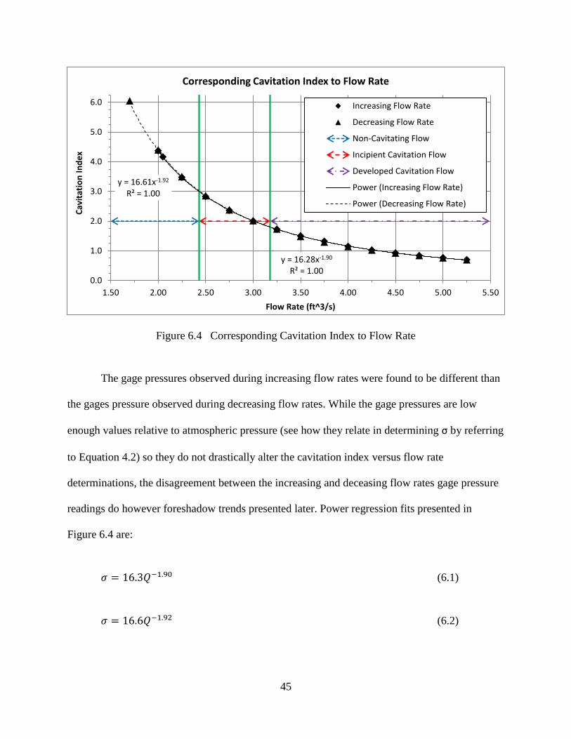
45
Figure 6.4 Corresponding Cavitation Index to Flow Rate
The gage pressures observed during increasing flow rates were found to be different than
the gages pressure observed during decreasing flow rates. While the gage pressures are low
enough values relative to atmospheric pressure (see how they relate in determining σ by referring
to Equation 4.2) so they do not drastically alter the cavitation index versus flow rate
determinations, the disagreement between the increasing and deceasing flow rates gage pressure
readings do however foreshadow trends presented later. Power regression fits presented in
Figure 6.4 are:
(6.1)
(6.2)
y = 16.28x-1.90 R² = 1.00
y = 16.61x-1.92 R² = 1.00
0.0
1.0
2.0
3.0
4.0
5.0
6.0
1.50 2.00 2.50 3.00 3.50 4.00 4.50 5.00 5.50
Cav
itat
ion
In
de
x
Flow Rate (ft^3/s)
Corresponding Cavitation Index to Flow Rate
Increasing Flow Rate
Decreasing Flow Rate
Non-Cavitating Flow
Incipient Cavitation Flow
Developed Cavitation Flow
Power (Increasing Flow Rate)
Power (Decreasing Flow Rate)
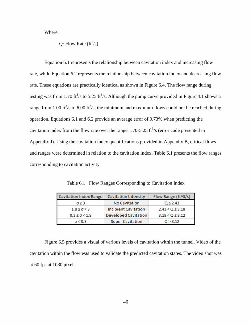
46
Where:
Q: Flow Rate (ft3/s)
Equation 6.1 represents the relationship between cavitation index and increasing flow
rate, while Equation 6.2 represents the relationship between cavitation index and decreasing flow
rate. These equations are practically identical as shown in Figure 6.4. The flow range during
testing was from 1.70 ft3/s to 5.25 ft
3/s. Although the pump curve provided in Figure 4.1 shows a
range from 1.00 ft3/s to 6.00 ft
3/s, the minimum and maximum flows could not be reached during
operation. Equations 6.1 and 6.2 provide an average error of 0.73% when predicting the
cavitation index from the flow rate over the range 1.70-5.25 ft3/s (error code presented in
Appendix J). Using the cavitation index quantifications provided in Appendix B, critical flows
and ranges were determined in relation to the cavitation index. Table 6.1 presents the flow ranges
corresponding to cavitation activity.
Table 6.1 Flow Ranges Corresponding to Cavitation Index
Figure 6.5 provides a visual of various levels of cavitation within the tunnel. Video of the
cavitation within the flow was used to validate the predicted cavitation states. The video shot was
at 60 fps at 1080 pixels.
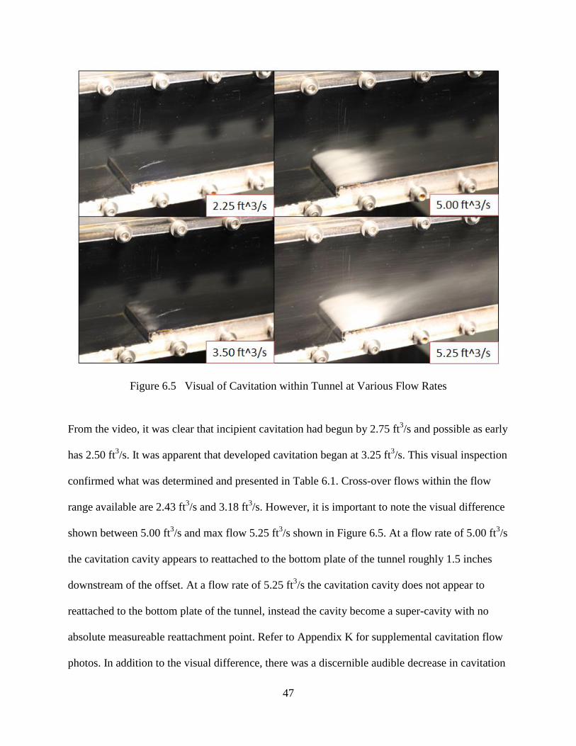
47
Figure 6.5 Visual of Cavitation within Tunnel at Various Flow Rates
From the video, it was clear that incipient cavitation had begun by 2.75 ft3/s and possible as early
has 2.50 ft3/s. It was apparent that developed cavitation began at 3.25 ft
3/s. This visual inspection
confirmed what was determined and presented in Table 6.1. Cross-over flows within the flow
range available are 2.43 ft3/s and 3.18 ft
3/s. However, it is important to note the visual difference
shown between 5.00 ft3/s and max flow 5.25 ft
3/s shown in Figure 6.5. At a flow rate of 5.00 ft
3/s
the cavitation cavity appears to reattached to the bottom plate of the tunnel roughly 1.5 inches
downstream of the offset. At a flow rate of 5.25 ft3/s the cavitation cavity does not appear to
reattached to the bottom plate of the tunnel, instead the cavity become a super-cavity with no
absolute measureable reattachment point. Refer to Appendix K for supplemental cavitation flow
photos. In addition to the visual difference, there was a discernible audible decrease in cavitation
48
noise from 5.00 to 5.25 ft3/s. It is believed that 5.25 ft
3/s was audibly quieter than 5.00 ft
3/s due
to the cavitation cavity which developed from 2.50 ft3/s to 5.00 ft
3/s broke loose from the bottom
plate. Once the cavity broke free, the bubbles were no longer collapsing 1.0-1.5 inches past the
offset local to the bottom plate but simply collapsing in the flow stream. This visual and audible
difference between 5.00 and 5.25 ft3/s was foreshadowing what would be confirmed later, that
maximum flow was actually the beginning of super cavitation. As such, two specific flow ranges
were to be scrutinized throughout the results analysis, 2.25-3.50 ft3/s for incipient cavitation and
5.00-5.25 for the transition from developed to super cavitation.
6.3 Root-Mean-Square Signal Strength Analysis
The simplest cavitation detection signal processing method is to correlate the strength of
the recorded signals to flow rate/cavitation index. Equation 5.1 was used to determine the RMS
value of all signals at recorded flow rates. Figures 6.6 – 6.8 present the RMS values of the
recorded signals for the top accelerometer, bottom accelerometer and AE sensor, respectively.
Refer to Appendix L for analysis code for both accelerometers and AE Sensor data. All
acceleration RMS values were determined from a 12 second time history, while all acoustic
emission RMS values were determined from an 8.5 second time history. Also, recorded signals
were from steady state measurements.
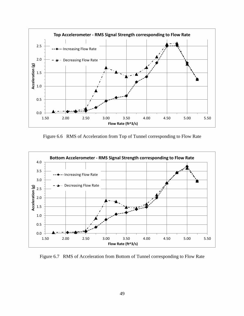
49
Figure 6.6 RMS of Acceleration from Top of Tunnel corresponding to Flow Rate
Figure 6.7 RMS of Acceleration from Bottom of Tunnel corresponding to Flow Rate
0.0
0.5
1.0
1.5
2.0
2.5
1.50 2.00 2.50 3.00 3.50 4.00 4.50 5.00 5.50
Acc
ele
rati
on
(g)
Flow Rate (ft^3/s)
Top Accelerometer - RMS Signal Strength corresponding to Flow Rate
Increasing Flow Rate
Decreasing Flow Rate
0.0
0.5
1.0
1.5
2.0
2.5
3.0
3.5
4.0
1.50 2.00 2.50 3.00 3.50 4.00 4.50 5.00 5.50
Acc
ele
rati
on
(g)
Flow Rate (ft^3/s)
Bottom Accelerometer - RMS Signal Strength corresponding to Flow Rate
Increasing Flow Rate
Decreasing Flow Rate
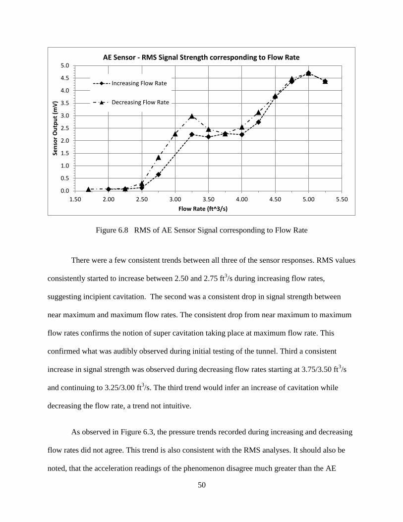
50
Figure 6.8 RMS of AE Sensor Signal corresponding to Flow Rate
There were a few consistent trends between all three of the sensor responses. RMS values
consistently started to increase between 2.50 and 2.75 ft3/s during increasing flow rates,
suggesting incipient cavitation. The second was a consistent drop in signal strength between
near maximum and maximum flow rates. The consistent drop from near maximum to maximum
flow rates confirms the notion of super cavitation taking place at maximum flow rate. This
confirmed what was audibly observed during initial testing of the tunnel. Third a consistent
increase in signal strength was observed during decreasing flow rates starting at 3.75/3.50 ft3/s
and continuing to 3.25/3.00 ft3/s. The third trend would infer an increase of cavitation while
decreasing the flow rate, a trend not intuitive.
As observed in Figure 6.3, the pressure trends recorded during increasing and decreasing
flow rates did not agree. This trend is also consistent with the RMS analyses. It should also be
noted, that the acceleration readings of the phenomenon disagree much greater than the AE
0.0
0.5
1.0
1.5
2.0
2.5
3.0
3.5
4.0
4.5
5.0
1.50 2.00 2.50 3.00 3.50 4.00 4.50 5.00 5.50
Sen
sor
Ou
tpu
t (m
V)
Flow Rate (ft^3/s)
AE Sensor - RMS Signal Strength corresponding to Flow Rate
Increasing Flow Rate
Decreasing Flow Rate

51
sensors in regards to the increasing versus decreasing flow rates. The disagreement between
increasing and decreasing flows suggest a hysteresis effect or a latent energy remaining in the
system during decreasing flow rates.
6.4 Auto-Correlation of Signals
The next step in the analysis was to confirm if the recorded signals had repeatable
characteristics. This was accomplished through the use of an auto-correlation, shown in
equation 5.2. Figures 6.9 – 6.11 present the results of the auto correlations of the top
acceleration, bottom acceleration and acoustic emissions respectively. Each figure contains three
separate flows, 2.00 ft3/s demonstrates a quiet non-cavitating flow, 2.75 ft
3/s demonstrates an
incipient cavitation and 5.00 ft3/s demonstrates a developed cavitation flow. Each auto-
correlation has been normalized via equation 5.3. Refer to Appendix L for analysis code for both
accelerometers and AE Sensor data.
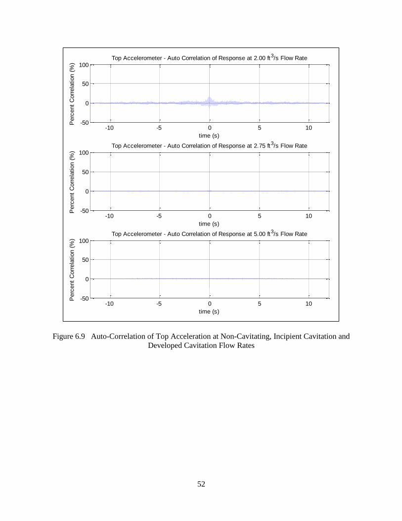
52
Figure 6.9 Auto-Correlation of Top Acceleration at Non-Cavitating, Incipient Cavitation and
Developed Cavitation Flow Rates
-10 -5 0 5 10-50
0
50
100Top Accelerometer - Auto Correlation of Response at 2.00 ft3/s Flow Rate
Perc
ent
Corr
ela
tion (
%)
time (s)
-10 -5 0 5 10-50
0
50
100Top Accelerometer - Auto Correlation of Response at 2.75 ft3/s Flow Rate
Perc
ent
Corr
ela
tion (
%)
time (s)
-10 -5 0 5 10-50
0
50
100Top Accelerometer - Auto Correlation of Response at 5.00 ft3/s Flow Rate
Perc
ent
Corr
ela
tion (
%)
time (s)
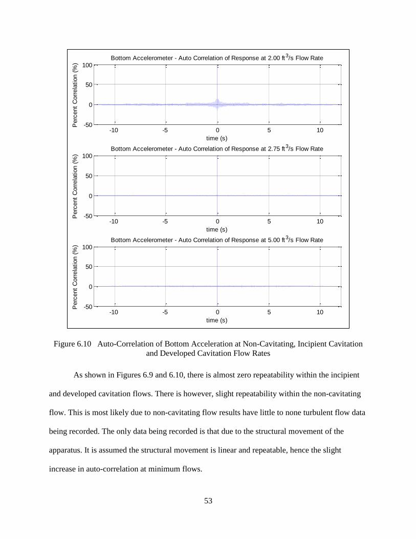
53
Figure 6.10 Auto-Correlation of Bottom Acceleration at Non-Cavitating, Incipient Cavitation
and Developed Cavitation Flow Rates
As shown in Figures 6.9 and 6.10, there is almost zero repeatability within the incipient
and developed cavitation flows. There is however, slight repeatability within the non-cavitating
flow. This is most likely due to non-cavitating flow results have little to none turbulent flow data
being recorded. The only data being recorded is that due to the structural movement of the
apparatus. It is assumed the structural movement is linear and repeatable, hence the slight
increase in auto-correlation at minimum flows.
-10 -5 0 5 10-50
0
50
100Bottom Accelerometer - Auto Correlation of Response at 2.00 ft3/s Flow Rate
Perc
ent
Corr
ela
tion (
%)
time (s)
-10 -5 0 5 10-50
0
50
100Bottom Accelerometer - Auto Correlation of Response at 2.75 ft3/s Flow Rate
Perc
ent
Corr
ela
tion (
%)
time (s)
-10 -5 0 5 10-50
0
50
100Bottom Accelerometer - Auto Correlation of Response at 5.00 ft3/s Flow Rate
Perc
ent
Corr
ela
tion (
%)
time (s)
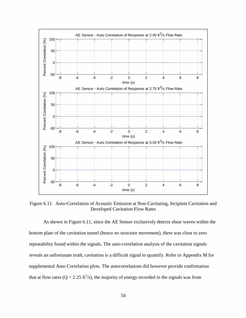
54
Figure 6.11 Auto-Correlation of Acoustic Emission at Non-Cavitating, Incipient Cavitation and
Developed Cavitation Flow Rates
As shown in Figure 6.11, since the AE Sensor exclusively detects shear waves within the
bottom plate of the cavitation tunnel (hence no structure movement), there was close to zero
repeatability found within the signals. The auto-correlation analysis of the cavitation signals
reveals an unfortunate truth, cavitation is a difficult signal to quantify. Refer to Appendix M for
supplemental Auto Correlation plots. The autocorrelations did however provide confirmation
that at flow rates (Q < 2.25 ft3/s), the majority of energy recorded in the signals was from
-8 -6 -4 -2 0 2 4 6 8-50
0
50
100AE Sensor - Auto Correlation of Response at 2.00 ft3/s Flow Rate
Perc
ent
Corr
ela
tion (
%)
time (s)
-8 -6 -4 -2 0 2 4 6 8-50
0
50
100AE Sensor - Auto Correlation of Response at 2.75 ft3/s Flow Rate
Perc
ent
Corr
ela
tion (
%)
time (s)
-8 -6 -4 -2 0 2 4 6 8-50
0
50
100AE Sensor - Auto Correlation of Response at 5.00 ft3/s Flow Rate
Perc
ent
Corr
ela
tion (
%)
time (s)
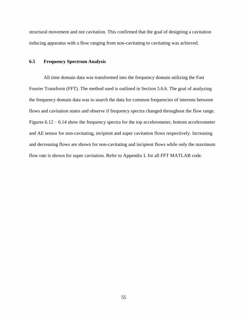
55
structural movement and not cavitation. This confirmed that the goal of designing a cavitation
inducing apparatus with a flow ranging from non-cavitating to cavitating was achieved.
6.5 Frequency Spectrum Analysis
All time domain data was transformed into the frequency domain utilizing the Fast
Fourier Transform (FFT). The method used is outlined in Section 5.6.6. The goal of analyzing
the frequency domain data was to search the data for common frequencies of interests between
flows and cavitation states and observe if frequency spectra changed throughout the flow range.
Figures 6.12 – 6.14 show the frequency spectra for the top accelerometer, bottom accelerometer
and AE sensor for non-cavitating, incipient and super cavitation flows respectively. Increasing
and decreasing flows are shown for non-cavitating and incipient flows while only the maximum
flow rate is shown for super cavitation. Refer to Appendix L for all FFT MATLAB code.
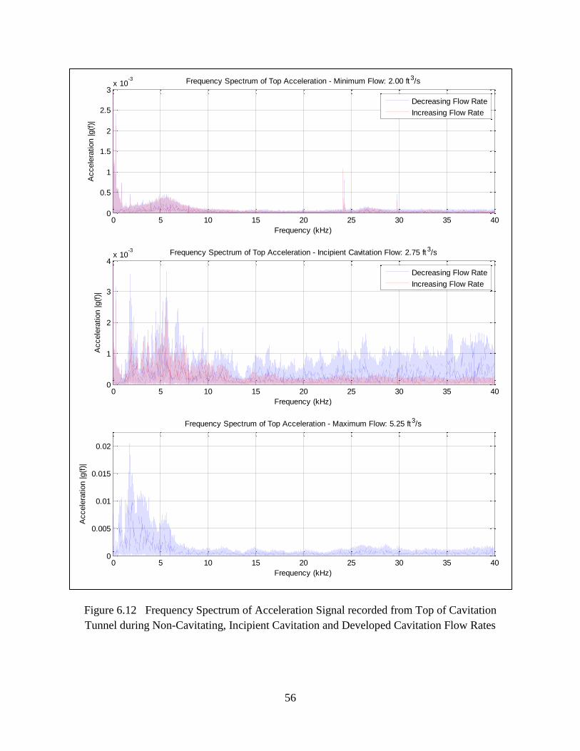
56
Figure 6.12 Frequency Spectrum of Acceleration Signal recorded from Top of Cavitation
Tunnel during Non-Cavitating, Incipient Cavitation and Developed Cavitation Flow Rates
0 5 10 15 20 25 30 35 400
0.5
1
1.5
2
2.5
3x 10
-3
Accele
ration |g(f
)|
Frequency (kHz)
Frequency Spectrum of Top Acceleration - Minimum Flow: 2.00 ft3/s
0 5 10 15 20 25 30 35 400
1
2
3
4x 10
-3
Accele
ration |g(f
)|
Frequency (kHz)
Frequency Spectrum of Top Acceleration - Incipient Cavitation Flow: 2.75 ft3/s
0 5 10 15 20 25 30 35 400
0.005
0.01
0.015
0.02
Accele
ration |g(f
)|
Frequency (kHz)
Frequency Spectrum of Top Acceleration - Maximum Flow: 5.25 ft3/s
Decreasing Flow Rate
Increasing Flow Rate
Decreasing Flow Rate
Increasing Flow Rate
57
Figure 6.13 Frequency Spectrum of Acceleration Signal recorded from Bottom of Cavitation
Tunnel during Non-Cavitating, Incipient Cavitation and Developed Cavitation Flow Rates
0 5 10 15 20 25 30 35 400
0.5
1
1.5
2
2.5
3x 10
-3
Accele
ration |g(f
)|
Frequency (kHz)
Frequency Spectrum of Bottom Acceleration - Minimum Flow: 2.00 ft3/s
0 5 10 15 20 25 30 35 400
1
2
3
4x 10
-3
Accele
ration |g(f
)|
Frequency (kHz)
Frequency Spectrum of Bottom Acceleration - Incipient Cavitation Flow: 2.75 ft 3/s
0 5 10 15 20 25 30 35 400
0.005
0.01
0.015
Accele
ration |g(f
)|
Frequency (kHz)
Frequency Spectrum of Bottom Acceleration - Maximum Flow: 5.25 ft3/s
Decreasing Flow Rate
Increasing Flow Rate
Decreasing Flow Rate
Increasing Flow Rate
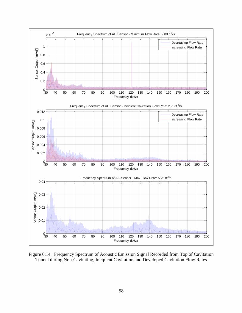
58
Figure 6.14 Frequency Spectrum of Acoustic Emission Signal Recorded from Top of Cavitation
Tunnel during Non-Cavitating, Incipient Cavitation and Developed Cavitation Flow Rates
30 40 50 60 70 80 90 100 110 120 130 140 150 160 170 180 190 2000
0.2
0.4
0.6
0.8
1
x 10-3
Frequency (kHz)
Sensor
Outp
ut
|mV
(f)|
Frequency Spectrum of AE Sensor - Minimum Flow Rate: 2.00 ft3/s
30 40 50 60 70 80 90 100 110 120 130 140 150 160 170 180 190 2000
0.002
0.004
0.006
0.008
0.01
0.012
Frequency (kHz)
Sensor
Outp
ut
|mV
(f)|
Frequency Spectrum of AE Sensor - Incipient Cavitation Flow Rate: 2.75 ft3/s
30 40 50 60 70 80 90 100 110 120 130 140 150 160 170 180 190 2000
0.01
0.02
0.03
0.04
Frequency (kHz)
Sensor
Outp
ut
|mV
(f)|
Frequency Spectrum of AE Sensor - Max Flow Rate: 5.25 ft3/s
Decreasing Flow Rate
Increasing Flow Rate
Decreasing Flow Rate
Increasing Flow Rate
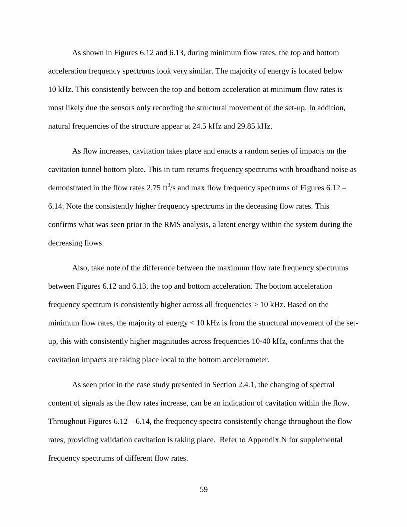
59
As shown in Figures 6.12 and 6.13, during minimum flow rates, the top and bottom
acceleration frequency spectrums look very similar. The majority of energy is located below
10 kHz. This consistently between the top and bottom acceleration at minimum flow rates is
most likely due the sensors only recording the structural movement of the set-up. In addition,
natural frequencies of the structure appear at 24.5 kHz and 29.85 kHz.
As flow increases, cavitation takes place and enacts a random series of impacts on the
cavitation tunnel bottom plate. This in turn returns frequency spectrums with broadband noise as
demonstrated in the flow rates 2.75 ft3/s and max flow frequency spectrums of Figures 6.12 –
6.14. Note the consistently higher frequency spectrums in the deceasing flow rates. This
confirms what was seen prior in the RMS analysis, a latent energy within the system during the
decreasing flows.
Also, take note of the difference between the maximum flow rate frequency spectrums
between Figures 6.12 and 6.13, the top and bottom acceleration. The bottom acceleration
frequency spectrum is consistently higher across all frequencies > 10 kHz. Based on the
minimum flow rates, the majority of energy < 10 kHz is from the structural movement of the set-
up, this with consistently higher magnitudes across frequencies 10-40 kHz, confirms that the
cavitation impacts are taking place local to the bottom accelerometer.
As seen prior in the case study presented in Section 2.4.1, the changing of spectral
content of signals as the flow rates increase, can be an indication of cavitation within the flow.
Throughout Figures 6.12 – 6.14, the frequency spectra consistently change throughout the flow
rates, providing validation cavitation is taking place. Refer to Appendix N for supplemental
frequency spectrums of different flow rates.
60
6.6 Normalized Frequency Spectrum Analysis
For low flow rates (Q < 2.25 ft3/s), the energy within the recorded signals is primarily
due to the structure and background noise from the non-cavitating flow. It was decided to
average the frequency spectrums of flow rates 2.00 ft3/s and 2.25 ft
3/s and use this spectrum to
normalize all the frequency spectrums. A detailed description of how the normalizing spectrum
was obtained is provided in Appendix O. The process of frequency spectrum normalization
outlined in Section 5.6.7 was followed. Figures 6.15 – 6.17 provide the normalized frequency
spectrums for the top accelerometer, bottom accelerometer and AE sensor for non-cavitating,
incipient and super cavitation respectively. Refer to Appendix L for normalized FFT MATLAB
code.
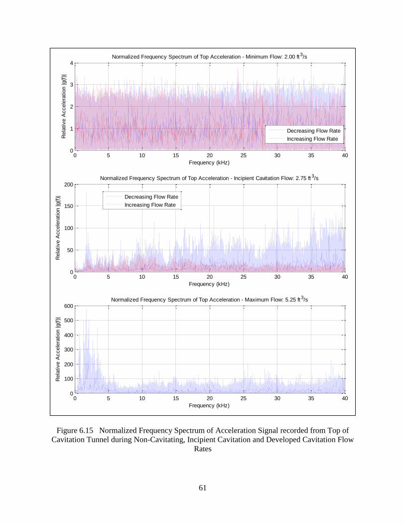
61
Figure 6.15 Normalized Frequency Spectrum of Acceleration Signal recorded from Top of
Cavitation Tunnel during Non-Cavitating, Incipient Cavitation and Developed Cavitation Flow
Rates
0 5 10 15 20 25 30 35 400
1
2
3
4R
ela
tive A
ccele
ration |g(f
)|
Frequency (kHz)
Normalized Frequency Spectrum of Top Acceleration - Minimum Flow: 2.00 ft3/s
Decreasing Flow Rate
Increasing Flow Rate
0 5 10 15 20 25 30 35 400
50
100
150
200
Rela
tive A
ccele
ration |g(f
)|
Frequency (kHz)
Normalized Frequency Spectrum of Top Acceleration - Incipient Cavitation Flow: 2.75 ft 3/s
Decreasing Flow Rate
Increasing Flow Rate
0 5 10 15 20 25 30 35 400
100
200
300
400
500
600
Rela
tive A
ccele
ration |g(f
)|
Frequency (kHz)
Normalized Frequency Spectrum of Top Acceleration - Maximum Flow: 5.25 ft3/s
62
Figure 6.16 Normalized Frequency Spectrum of Acceleration Signal recorded from Bottom of
Cavitation Tunnel during Non-Cavitating, Incipient Cavitation and Developed Cavitation Flow
Rates
0 5 10 15 20 25 30 35 400
1
2
3
4R
ela
tive A
ccele
ration |g(f
)|
Frequency (kHz)
Normalized Frequency Spectrum of Bottom Acceleration - Minimum Flow: 2.00 ft3/s
Decreasing Flow Rate
Increasing Flow Rate
0 5 10 15 20 25 30 35 400
50
100
150
Rela
tive A
ccele
ration |g(f
)|
Frequency (kHz)
Normalized Frequency Spectrum of Bottom Acceleration - Incipient Cavitation Flow: 2.75 ft 3/s
Decreasing Flow Rate
Increasing Flow Rate
0 5 10 15 20 25 30 35 400
100
200
300
400
500
600
Rela
tive A
ccele
ration |g(f
)|
Frequency (kHz)
Normalized Frequency Spectrum of Bottom Acceleration - Maximum Flow: 5.25 ft3/s
63
Figure 6.17 Normalized Frequency Spectrum of Acoustic Emission recorded from Bottom of
Cavitation Tunnel during Non-Cavitating, Incipient Cavitation and Developed Cavitation Flow
Rates
30 40 50 60 70 80 90 100 110 120 130 140 150 160 170 180 190 2000
1
2
3
4
Frequency (kHz)
Rela
tive S
ensor
Outp
ut
|mV
(f)|
Normalized Frequency Spectrum of AE Sensor - Minimum Flow Rate: 2.00 ft3/s
30 40 50 60 70 80 90 100 110 120 130 140 150 160 170 180 190 2000
50
100
150
200
250
300
Frequency (kHz)
Rela
tive S
ensor
Outp
ut
|mV
(f)|
Normalized Frequency Spectrum of AE Sensor - Incipient Cavitation Flow Rate: 2.75 ft 3/s
30 40 50 60 70 80 90 100 110 120 130 140 150 160 170 180 190 2000
500
1000
1500
Frequency (kHz)
Rela
tive S
ensor
Outp
ut
|mV
(f)|
Normalized Frequency Spectrum of AE Sensor - Max Flow Rate: 5.25 ft3/s
Decreasing Flow Rate
Increasing Flow Rate
Decreasing Flow Rate
Increasing Flow Rate
64
As shown in Figures 6.15 – 6.17, the minimum flow rates frequency spectrums are flat
(consistent amplitude across the spectrum). It was the flow rates 2.00 – 2.25 ft3/s which were
used to normalize all the frequency spectrums, thus the minimum flows relative frequency
spectrums being flat provides confirmation the normalization has worked effectively to remove
non-cavitation influences on the spectrums. It is important to notice the y-axis on Figures 6.15 –
6.17. The y-axis are not |magnitude(f)|, but relative |magnitude(f)|. This relative |magnitude(f)|
unit is due to the resulting magnitude being dependent on the low flow frequency spectrums but
as all frequency spectrums were normalized by the same low flow frequency spectrum,
comparing different flows and observing specific frequencies with particularly high magnitudes
is still a valid metric for analysis. It important however to not use normalized spectrums in
absolute terms.
As shown in the prior Figures 6.15 – 6.17, the normalized frequency spectrums
reinforced the fact that broadband noise is being introduced into the system from cavitation
impacts on the bottom plate. As seen in prior, its important to note that the bottom accelerometer
consistently recorded higher acceleration that the top accelerometer at non-cavitating flows.
Finally, the changing of frequency spectra and amplitude throughout the with cavitation states is
clearly demonstrated. Refer to Appendix P for supplemental normalized frequency spectrums.
65
6.7 Coherence between Top and Bottom Acceleration
The first step when utilizing equation 5.6 to determine the coherence between two signals
is to determine the type, length and overlap of the window applied to the data. For all results
presented in this section, a Hanning window of length 215
was used with an overlap of 214
. For a
detailed explanation of how this window, length and overlap were chosen and how these choices
influence the coherence results, refer to Appendix Q. Figure 6.18 presents the coherence of the
top and bottom acceleration readings at flow rates 2.00 ft3/s, 2.75 ft
3/s and 5.25 ft
3/s. Refer to
Appendix L for coherence MATLAB code.
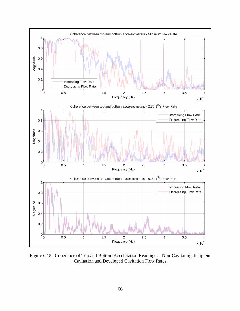
66
Figure 6.18 Coherence of Top and Bottom Acceleration Readings at Non-Cavitating, Incipient
Cavitation and Developed Cavitation Flow Rates
0 0.5 1 1.5 2 2.5 3 3.5 4
x 104
0
0.2
0.4
0.6
0.8
1
Frequency (Hz)
Magnitude
Coherence between top and bottom accelerometers - Minimum Flow Rate
0 0.5 1 1.5 2 2.5 3 3.5 4
x 104
0
0.2
0.4
0.6
0.8
1
Frequency (Hz)
Magnitude
Coherence between top and bottom accelerometers - 2.75 ft3/s Flow Rate
0 0.5 1 1.5 2 2.5 3 3.5 4
x 104
0
0.2
0.4
0.6
0.8
1
Frequency (Hz)
Magnitude
Coherence between top and bottom accelerometers - 5.00 ft3/s Flow Rate
Increasing Flow Rate
Decreasing Flow Rate
Increasing Flow Rate
Decreasing Flow Rate
Increasing Flow Rate
Decreasing Flow Rate
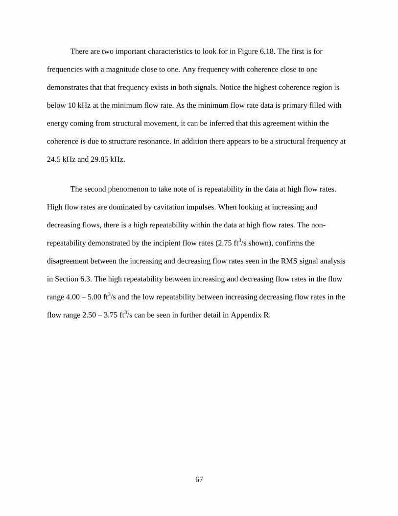
67
There are two important characteristics to look for in Figure 6.18. The first is for
frequencies with a magnitude close to one. Any frequency with coherence close to one
demonstrates that that frequency exists in both signals. Notice the highest coherence region is
below 10 kHz at the minimum flow rate. As the minimum flow rate data is primary filled with
energy coming from structural movement, it can be inferred that this agreement within the
coherence is due to structure resonance. In addition there appears to be a structural frequency at
24.5 kHz and 29.85 kHz.
The second phenomenon to take note of is repeatability in the data at high flow rates.
High flow rates are dominated by cavitation impulses. When looking at increasing and
decreasing flows, there is a high repeatability within the data at high flow rates. The non-
repeatability demonstrated by the incipient flow rates (2.75 ft3/s shown), confirms the
disagreement between the increasing and decreasing flow rates seen in the RMS signal analysis
in Section 6.3. The high repeatability between increasing and decreasing flow rates in the flow
range 4.00 – 5.00 ft3/s and the low repeatability between increasing decreasing flow rates in the
flow range 2.50 – 3.75 ft3/s can be seen in further detail in Appendix R.
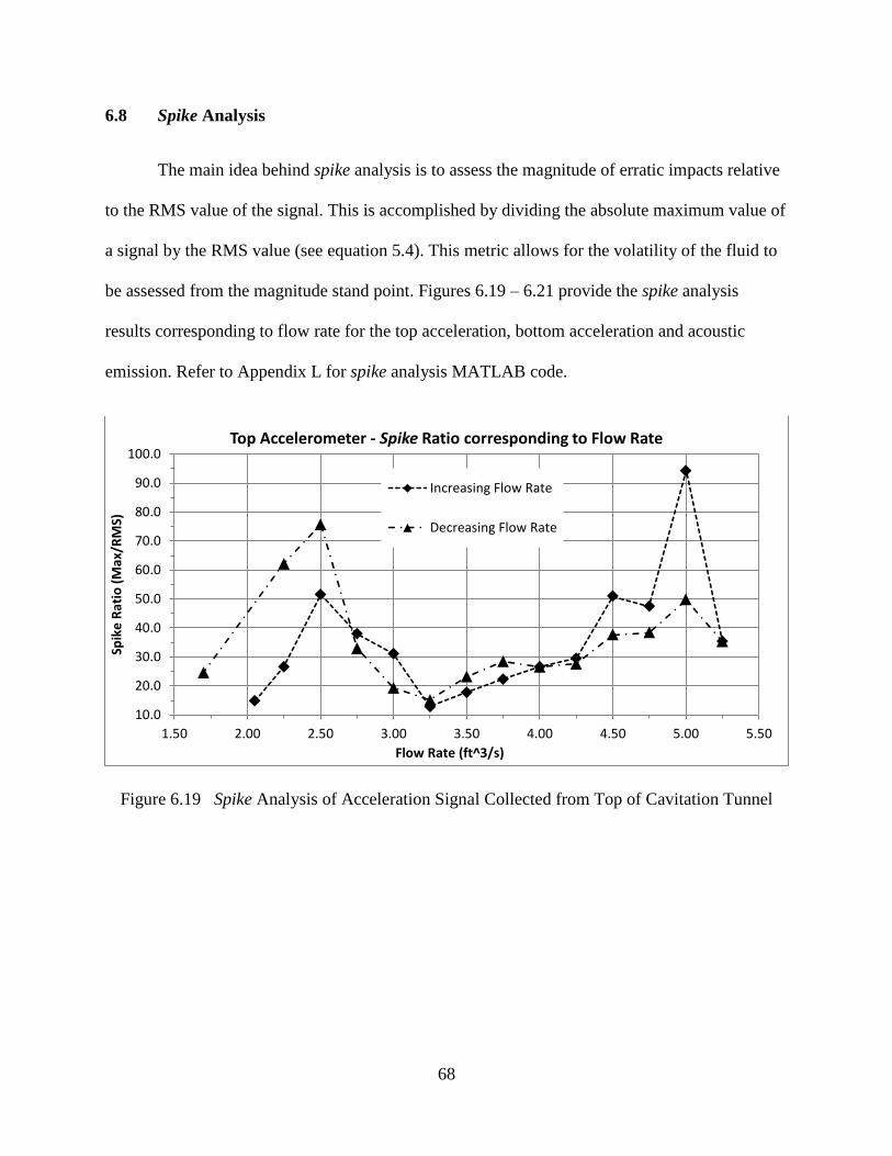
68
6.8 Spike Analysis
The main idea behind spike analysis is to assess the magnitude of erratic impacts relative
to the RMS value of the signal. This is accomplished by dividing the absolute maximum value of
a signal by the RMS value (see equation 5.4). This metric allows for the volatility of the fluid to
be assessed from the magnitude stand point. Figures 6.19 – 6.21 provide the spike analysis
results corresponding to flow rate for the top acceleration, bottom acceleration and acoustic
emission. Refer to Appendix L for spike analysis MATLAB code.
Figure 6.19 Spike Analysis of Acceleration Signal Collected from Top of Cavitation Tunnel
10.0
20.0
30.0
40.0
50.0
60.0
70.0
80.0
90.0
100.0
1.50 2.00 2.50 3.00 3.50 4.00 4.50 5.00 5.50
Spik
e R
atio
(M
ax/R
MS)
Flow Rate (ft^3/s)
Top Accelerometer - Spike Ratio corresponding to Flow Rate
Increasing Flow Rate
Decreasing Flow Rate
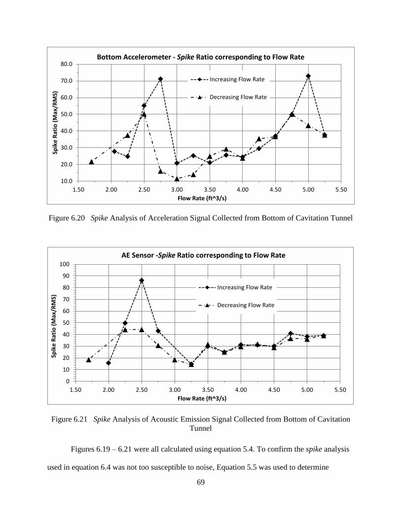
69
Figure 6.20 Spike Analysis of Acceleration Signal Collected from Bottom of Cavitation Tunnel
Figure 6.21 Spike Analysis of Acoustic Emission Signal Collected from Bottom of Cavitation
Tunnel
Figures 6.19 – 6.21 were all calculated using equation 5.4. To confirm the spike analysis
used in equation 6.4 was not too susceptible to noise, Equation 5.5 was used to determine
10.0
20.0
30.0
40.0
50.0
60.0
70.0
80.0
1.50 2.00 2.50 3.00 3.50 4.00 4.50 5.00 5.50
Spik
e R
atio
(M
ax/R
MS)
Flow Rate (ft^3/s)
Bottom Accelerometer - Spike Ratio corresponding to Flow Rate
Increasing Flow Rate
Decreasing Flow Rate
0
10
20
30
40
50
60
70
80
90
100
1.50 2.00 2.50 3.00 3.50 4.00 4.50 5.00 5.50
Spik
e R
atio
(M
ax/R
MS)
Flow Rate (ft^3/s)
AE Sensor -Spike Ratio corresponding to Flow Rate
Increasing Flow Rate
Decreasing Flow Rate
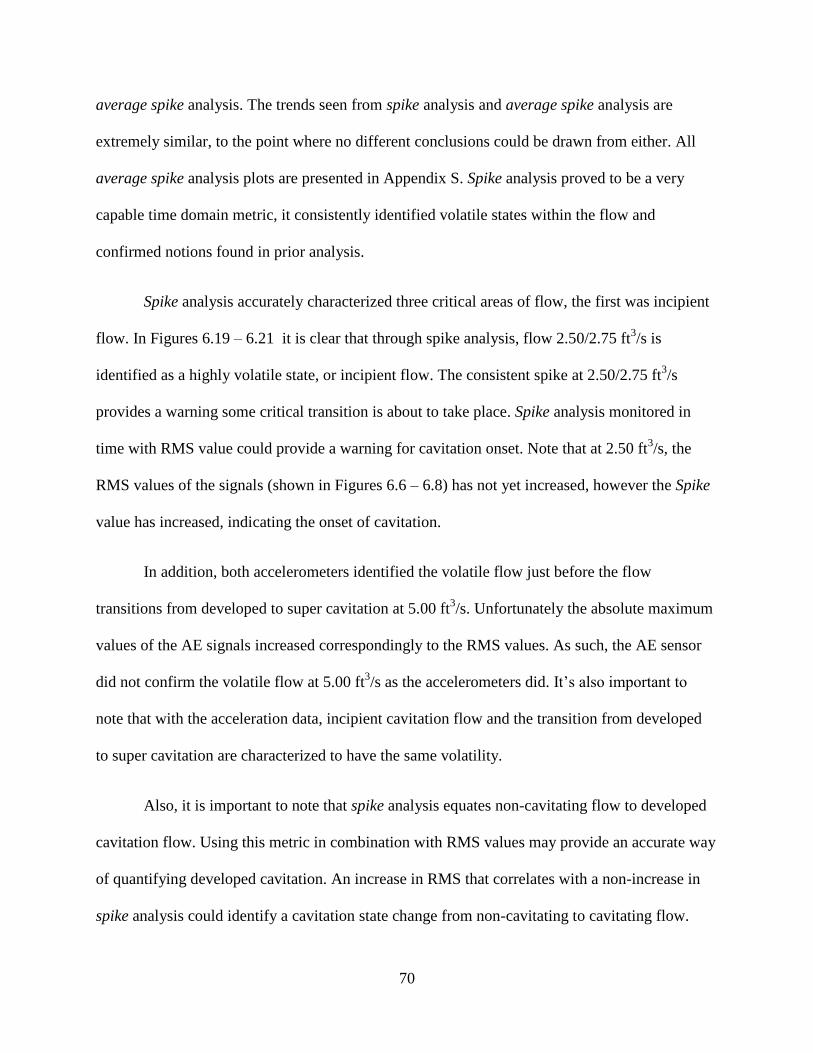
70
average spike analysis. The trends seen from spike analysis and average spike analysis are
extremely similar, to the point where no different conclusions could be drawn from either. All
average spike analysis plots are presented in Appendix S. Spike analysis proved to be a very
capable time domain metric, it consistently identified volatile states within the flow and
confirmed notions found in prior analysis.
Spike analysis accurately characterized three critical areas of flow, the first was incipient
flow. In Figures 6.19 – 6.21 it is clear that through spike analysis, flow 2.50/2.75 ft3/s is
identified as a highly volatile state, or incipient flow. The consistent spike at 2.50/2.75 ft3/s
provides a warning some critical transition is about to take place. Spike analysis monitored in
time with RMS value could provide a warning for cavitation onset. Note that at 2.50 ft3/s, the
RMS values of the signals (shown in Figures 6.6 – 6.8) has not yet increased, however the Spike
value has increased, indicating the onset of cavitation.
In addition, both accelerometers identified the volatile flow just before the flow
transitions from developed to super cavitation at 5.00 ft3/s. Unfortunately the absolute maximum
values of the AE signals increased correspondingly to the RMS values. As such, the AE sensor
did not confirm the volatile flow at 5.00 ft3/s as the accelerometers did. It’s also important to
note that with the acceleration data, incipient cavitation flow and the transition from developed
to super cavitation are characterized to have the same volatility.
Also, it is important to note that spike analysis equates non-cavitating flow to developed
cavitation flow. Using this metric in combination with RMS values may provide an accurate way
of quantifying developed cavitation. An increase in RMS that correlates with a non-increase in
spike analysis could identify a cavitation state change from non-cavitating to cavitating flow.
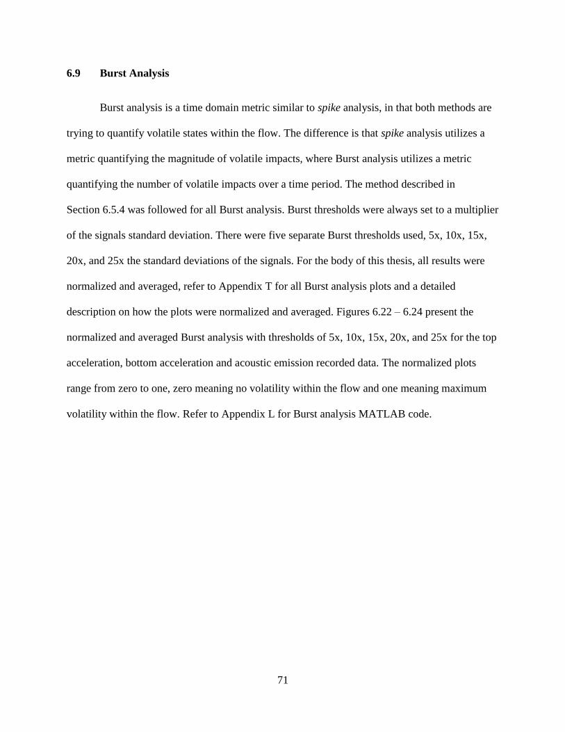
71
6.9 Burst Analysis
Burst analysis is a time domain metric similar to spike analysis, in that both methods are
trying to quantify volatile states within the flow. The difference is that spike analysis utilizes a
metric quantifying the magnitude of volatile impacts, where Burst analysis utilizes a metric
quantifying the number of volatile impacts over a time period. The method described in
Section 6.5.4 was followed for all Burst analysis. Burst thresholds were always set to a multiplier
of the signals standard deviation. There were five separate Burst thresholds used, 5x, 10x, 15x,
20x, and 25x the standard deviations of the signals. For the body of this thesis, all results were
normalized and averaged, refer to Appendix T for all Burst analysis plots and a detailed
description on how the plots were normalized and averaged. Figures 6.22 – 6.24 present the
normalized and averaged Burst analysis with thresholds of 5x, 10x, 15x, 20x, and 25x for the top
acceleration, bottom acceleration and acoustic emission recorded data. The normalized plots
range from zero to one, zero meaning no volatility within the flow and one meaning maximum
volatility within the flow. Refer to Appendix L for Burst analysis MATLAB code.
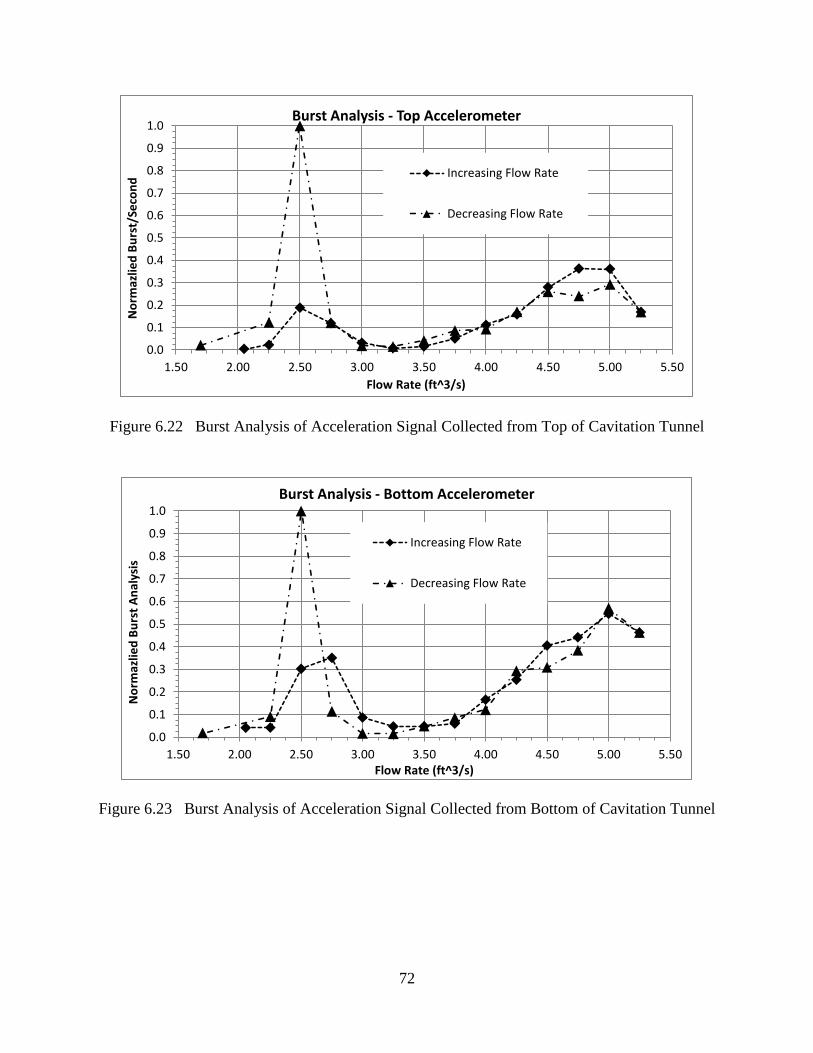
72
Figure 6.22 Burst Analysis of Acceleration Signal Collected from Top of Cavitation Tunnel
Figure 6.23 Burst Analysis of Acceleration Signal Collected from Bottom of Cavitation Tunnel
0.0
0.1
0.2
0.3
0.4
0.5
0.6
0.7
0.8
0.9
1.0
1.50 2.00 2.50 3.00 3.50 4.00 4.50 5.00 5.50
No
rmaz
lied
Bu
rst/
Seco
nd
Flow Rate (ft^3/s)
Burst Analysis - Top Accelerometer
Increasing Flow Rate
Decreasing Flow Rate
0.0
0.1
0.2
0.3
0.4
0.5
0.6
0.7
0.8
0.9
1.0
1.50 2.00 2.50 3.00 3.50 4.00 4.50 5.00 5.50
No
rmaz
lied
Bu
rst
An
alys
is
Flow Rate (ft^3/s)
Burst Analysis - Bottom Accelerometer
Increasing Flow Rate
Decreasing Flow Rate
73
Figure 6.24 Burst Analysis of Acoustic Emission Collected from Bottom of Cavitation Tunnel
Burst analysis consistently identified, with increasing flow, volatility at 2.50 ft3/s. As
identified in many prior metrics, 2.50 ft3/s is the start of incipient cavitation flow. In addition, the
accelerometers identified much higher volatility in the decreasing flow rate, inferring cavitation
continuing to further down the flow range. This phenomenon which has also been identified in
multiple prior metrics was not confirmed with the acoustic emission recordings. The AE sensor
however provided data inferring the increasing and decreasing flow rates had the same volatility
at 2.50 ft3/s. This is an anomaly among all the metrics utilized.
Also, both of the acceleration readings provided confirmation of the flow state change
from 5.00 – 5.25 ft3/s from developed to super cavitation. However, the acoustic emission sensor
did not identify this state change. The AE sensor did however accurately depict the increasing
volatility in the flow from 3.50 – 5.00 ft3/s.
0.0
0.1
0.2
0.3
0.4
0.5
0.6
0.7
0.8
0.9
1.0
1.50 2.00 2.50 3.00 3.50 4.00 4.50 5.00 5.50
No
rmaz
lied
Bu
rst/
Seco
nd
Flow Rate (ft^3/s)
Burst Analysis - AE Sensor
Increasing Flow Rate
Decreasing Flow Rate
74
CHAPTER 7
CONCLUSIONS AND RECOMMENDATIONS FOR FUTURE WORK
7.1 Conclusions
A controllable laboratory experiment consisting of a cavitation inducing tunnel was
conceived, designed and built for characterization of cavitation signals. Instrumentation to
confirm cavitation and record vibroacoustic activity included a pressure transducer, two
accelerometers and an AE sensor. The flow range of the laboratory set-up provided non-
cavitating flow (quiet) at the low end of the range, and super cavitating flow (loud) at the
maximum flow.
Initial characterization of the signals included correlating RMS values to specific flow
rates and cavitation indexes. The RMS analysis revealed several characteristics of the flow.
These included, incipient cavitation taking place at approximately 2.50 ft3/s and super cavitation
taking place at maximum flow, 5.25 ft3/s. RMS signal analysis also revealed that once cavitation
begins within a flow at a certain threshold during increasing flow, cavitation can then happen
lower than the initial threshold when decreasing flow.
All signals were checked for repeatability via autocorrelations. It was determined that
cavitation is a non-repeatable signal. However, the autocorrelations did provide confirmation that
at flow rates (Q < 2.25 ft3/s), the majority of energy recorded in the signals was from structural
movement and not cavitation; thus the goal of designing a cavitation inducing apparatus with a
flow range ranging from non-cavitating to cavitating was achieved. This was further
substantiated by the results of the coherence between the top and bottom accelerometers. At low
75
flow rates, there was a high degree of coherence agreement in the low frequency range,
confirming the repeatability in the signals and the notion that the majority of energy in the
signals recorded at low flow rates was primarily due to structural movement.
All signals were transformed into the frequency domain to check for changes in
frequency spectra at different flow rates. As demonstrated in prior cavitation monitoring work,
the frequency spectra changed throughout the cavitation states, inferring cavitation taking place
within the apparatus. This was further substantiated by frequency normalization analysis, which
removed structural influence on the frequency spectra. The results of frequency normalization
again confirm that the frequency spectra changed throughout the flow range and subsequently
cavitation changed throughout the flow range.
Spike and Burst time domain metrics were further developed due to difficulty in
quantifying frequency domain results. Both time domain metrics developed were designed to
quantify volatility within the flow. Volatility is a useful metric to quantify when cavitation states
are going to change (i.e. incipient cavitation). Both metrics were able to identify incipient
cavitation, the transition from developed to super cavitation and confirm the notion that
cavitation takes place lower in the flow range with decreasing flow rate versus increasing flow
rate.
The combination of RMS signal analysis, autocorrelation of signals, coherence of top and
bottom accelerometer signals, frequency domain analysis, spike analysis and Burst analysis
provides a validated framework for non-intrusive cavitation detection. Within the cavitation
inducing apparatus developed for this project, it was predicted and validated that incipient
cavitation took place at 2.50ft3/s. In addition, it was experimentally determined that the transition
76
from developed to super cavitation takes place from 5.00 ft3/s to 5.25 ft
3/s, when the cavitation
cavity developed from 2.50 – 5.00 ft3/s breaks loose from the bottom plate.
7.2 Future Work
The accomplishments of this project are a small step in the long term goals of real-time
CHM of large scale hydropower turbines. This project’s developed metrics for non-intrusive
cavitation detection were proven on a simple and quantifiable cavitation inducing apparatus. The
next step in the process is to apply the metrics to data taken from a known cavitating hydropower
turbine. Such an opportunity may exist in the Summer/Fall of 2013 at the Judge Francis Carr
Hydro Power Plant in Northern California. Carr Power Plant consists of two Francis turbine
generators units with a total capacity of 154.4 MW [32]. The turbine runners are currently
experiencing severe cavitation. There is a site-visit currently being planned for a team of
engineers from the U.S. Bureau of Reclamation office in Denver to travel to the site and record
accelerometer and acoustic emission readings from the turbine at various flow rates and
generator load levels. A wireless data acquisition system will be used to collect data from the
rotating shaft which connects the runner of the turbine to the generator, much in the same fashion
as the case study presented in Section 2.4.1. All data collected from the site will be analyzed
using the metrics created, validated and outlined in Chapter 5.
There is confidence the metrics here will lead to conclusions as to which operating
conditions at Carr Powerplant are causing the cavitation. The use of these metrics will ultimately
lead to restrictions on flow rates and generator loading. These restrictions however will lead to
less downtime, less unplanned maintenance and ultimately higher electrical production and profit
margins for Carr Powerplant.

77
LIST OF ABBREVIATIONS AND SYMBOLS
Abbreviations
CHM: Condition Health Monitoring
HQ: Hydro-Quebec
TVA: Tennessee Valley Authority
EPFL: Swiss Federal Institute of Technology, Lausanne
UPC: Technical University of Catalonia
USBR: U.S. Bureau of Reclamation
FT1: Francis Turbine 1
FT2: Francis Turbine 2
HHP: High Head Pump
AE: Acoustic Emission
GUI: Graphical User Interface
ACSII: American Standard Code for Information Exchange
RMS: Root Mean Square
FFT: Fast Fourier Transform
fps: frames per second
Symbols
Zb: Number of turbine runner blades
Zv: Number of turbine Guide Vanes
N: Turbine rotational speed (rpm)
ff: Turbine fundamental frequency
fb: Blade passing frequency
fv: Guide vane passing frequency
σ: Cavitation Index
AT: Cross-Sectional area of Cavitation Tunnel (before offset)
AS: Cross-Section area of Cavitation Tunnel at offset
Q: Flow rate
Qmin: Minimum flow rate
Qmax: Maximum flow rate
V: Velocity
Vmin: Minimum Velocity
Vmax: Maximum Velocity
Po: Reference pressure – Pressure in free stream flow at offset
Pa: Atmospheric pressure
Pg: Gage pressure
: Density
78
Symbols (continued)
Vo: Average fluid velocity in free stream flow at offset
Re: Reynolds Number
DH: Hydraulic diameter
v: Kinematic viscosity
P: Perimeter
x(t): Real valued time domain signal
y(t): Real valued time domain signal
Cxy: Coherence between two real-valued signals
Gxy: Cross spectral density of two real valued signals
Gxx: Auto-spectral density of x
Gyy: Auto-spectral density of y
79
REFERENCES
[1] “U.S. Energy Information Administration – EIA – Independent Statistics and
Analysis.”Electric Power Monthly. N.p., n.d. Web. 05 Nov. 2012.
<http://www.eia.gov/electricity/monthly/>.
[2] “HydroResearchFoundation.” Hydro Research Foundation. N.p., n.d. Web. 05 Nov.
2012. <http://www.hydrofoundation.org/hydropower-education.html>.
[3] Bourdon P., Farhat M., Mossoba Y., Lavigne P., “Hydro Turbine Profitability and
Cavitation Erosion”, Hydro-Quebec. Montreal, Quebec, Canada
[4] Mossoba, Y., “Efficient Cavitation Detection Technology for Optimizing Hydro Turbines
Operation and Maintenance”, Hydro-Quebec Generation. Montreal, Quebec, Canada
[5] "How Waterpower Works." How Waterpower Works. N.p., n.d. Web. 14 Mar. 2013.
<http://www.xeneca.com/benefits/how_hyrdro_power_works.html>.
[6] "What Is Kaplan Turbine? Propeller Turbine. Types of Hydraulic Turbines." Brighthub
Engineering. N.p., 27 Nov. 2009. Web. 14 Mar. 2013.
<http://www.brighthubengineering.com/fluid-mechanics-hydraulics/27426-hydraulic-
turbines-kaplan-turbine/>.
[7] Mossoba Y. (Principal Investigator), Wilson A. (Technology Cooridator), 2009,
“Technology Review On-Line Cavitation Monitoring”, Hydro-Quebec. Montreal,
Quebec, Canada
[8] Mossoba Y., Bourdon P., October 1999, “Sharing Experience with Cavitation Repair,
Monitoring”, Hydro Review, pp. 16-22
[9] Harrison M., 1952, “An Experimental Study of Single Bubble Cavitation Noise”, The
Journal of the Acoustical Society of America, Volume 24, No.6, November 1952, pp.
776-782
[10] Franc, Jean-Pierre, and Jean-Marie Michel. Fundamentals of Cavitation. Dordrecht:
Kluwer Academic, 2004. Print.
[11] Bajic, B., 2008 , “Multidimensional Method and Simple Methods for Cavitation
Diagnostics and Monitoring”, Seminar on the State of the Art Monitoring Systems
applied to Rotating Machines, November 2008
[12] D. Mba and Raj B. K. N. Rao, 2006, “Development of Acoustic Emission Technology for
Condition Monitoring and Diagnosis of Rotating Machines: Bearings, Pumps, Gearboxes,
80
Engines, and Rotating Structures”, The Shock and Vibration Digest, Vol. 38, No.1, Jan
2006, pp.3-16
[13] Escaler X., Egusquiza E., Mebarki T., Technical University of Catalonia-UPC, Farhat
M., Avellan F., Swiss Federal Institute of Technology-EPFL, 2002, “Field Assessment of
Cavitation Detection Methods in Hydropower Plants”, Proceedings of the XXIst IAHR
Symposium on Hydraulic Machinery and Systems. Lausanne, Switzerland
[14] March P., Jones K., 1991, “Laboratory and Field Experience with Cavitation Monitoring
of Hydroturbines”, Waterpower Conference 1991
[15] Abbot, P.A., Gedney C.J., Greeley D.S., “Cavitation Monitoring of Two Axial-Flow
Hydroturbines using Novel Acoustic and Vibration Methods”, Atlantic Applied Research
Corportation, Burlington, MA, 01803, U.S.
[16] Bajic, B., 2003, “Methods for Vibro-Acoustic Diagnostics of Turbine Cavitation”,
Journal of Hydraulic Research. Vol 41, 2003, No.1, pp. 87-96
[17] Bajic B., Keller A., 1996, “Spectrum Normalization Method in Vibro-Acoustical
Diagnostic Measurements of Hydroturbine Cavitation”, Journal of Fluids Engineering,
Vol.118, December 1996, pp. 756-761
[18] Bourdon P., Farhat M., 1998, “Extending Repair Intervals of Hydro Turbines by
Mitigating Cavitation Erosion”, CEA Electricity Conference & Exposition. Toronto,
Canada
[19] Farhat M., Bourdon P., Lavigne P., Simoneau R., 1997, “The Hydrodynamic
Aggressiveness of Cavitating Flows in Hydro Turbines”, ASME Fluids Engineering
Division Summer Meeting
[20] Wenjie C., “Acoustic Method for Measuring Cavitation and Impulse Counting of it’s
Noise”, Dailian Institute of Technology, Translated by: U.S. Bureau of Reclamation
1983.
[21] Bourdon P., Farhat M., Simoneau R., Hydro-Quebec, Pereira F., Dupont P., Avellan F.,
IMHEF/EPFL, Dorey J.M., Electricite de France, 1996, “Cavitation Erosion Prediction
on Francis Turbines-Part 1 Measurements on the Prototype”, Hydraulic Machinery and
Cavitation, pp. 534-543
[22] Bourdon P., Simoneau R., Avellan F., June 1993, “Hydraulic Turbine Cavitation Pitting
Detection by Monitoring Runner Vibration”, Report for: Canadian Electrical Association,
Prepared by: Hydro-Quebec
81
[23] Mossoba Y., Hydro Quebec, Bourdon P., Farhat M., Simoneau R., Institut de Recherche
d’Hydro-Quebec, “Solutions dealing with the Cavitation Erosion Damages in Hydro
Turbines”.
[24] Escaler X., Egusquiza E., Technical University of Catalonia-UPC, Farhat M., Avellan F.,
Swiss Federal Institute of Technology-EPFL, 2004, “Cavitation Erosion Prediction in
Hydro Turbines from Onboard Vibrations”, 22nd
IAHR Symposium on Hydraulic
Machinery and Systems. Stockholm, Sweden
[25] Escaler X., Egusquiza E., Technical University of Catalonia-UPC, Farhat M., Avellan F.,
Swiss Federal Institute of Technology-EPFL, 2003, “Vibration Cavitation Detection
using Onboard Measurements”, Fifth International Symposium on Cavitation. Osaka,
Japan
[26] United States of America. Department of the Interior. Bureau of Reclamation. Cavitation
in Chutes and Spillways. By Henry T. Falvey. N.p.: Water Resources Technical
Publication, n.d. Print. Engineering Monograph No.42.
[27] "Pressure Transmitter Honeywell Data Instruments Model BL." Pressure Transmitter
Honeywell Data Instruments Model BL. N.p., n.d. Web. 14 Mar. 2013.
<http://www.intertechnology.com/Honeywell_Data_Inst/Honeywell_BL.html>.
[28] "MODEL 1000/A/BMINIATURE PREMIUM 10 OR 1.5 MV/G
ACCELEROMETER."MISTRAS NDT Products & Systems. N.p., n.d. Web. 14 Mar.
2013.
<http://www.mistrasgroup.com/products/solutions/vibration/accelerometers/1000.aspx>.
[29] "SE9125-M." DECI. N.p., n.d. Web. 14 Mar. 2013.
<http://www.deci.com/se9125m.pdf>.
[30] "WaveBook/516E." Ethernet-Based Portable High-Speed Waveform Acquisition. N.p.,
n.d. Web. 14 Mar. 2013. <http://www.mccdaq.com/products/wavebook516e.htm>.
[31] "Data Acquisition System Laboratory." DASYLab. N.p., n.d. Web. 14 Mar. 2013.
<http://www.dasylab.com/>.
[32] "Judge Francis Carr Powerplant." U.S. Bureau of Reclamation. N.p., 13 May 2009. Web.
14 Mar. 2013.
<http://www.usbr.gov/projects/Powerplant.jsp?fac_Name=Judge+Francis+Carr+Powerpl
ant>.
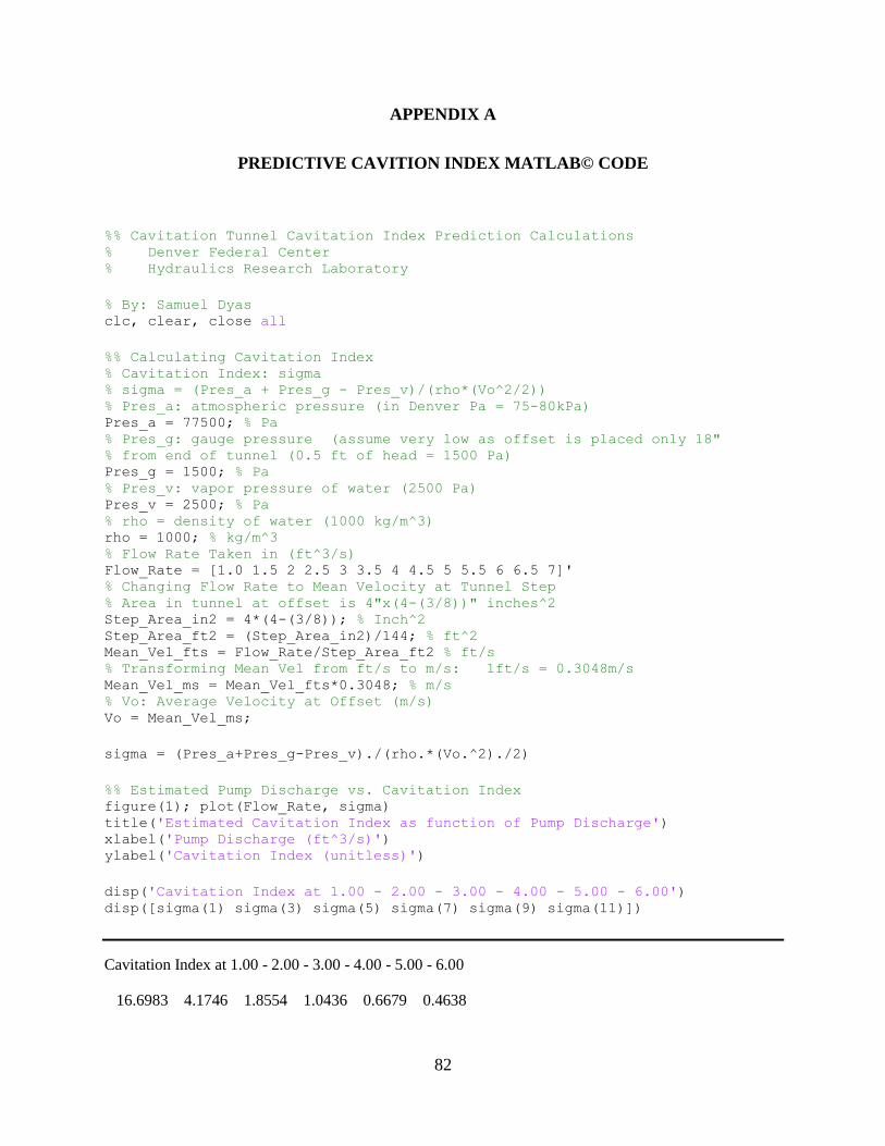
82
APPENDIX A
PREDICTIVE CAVITION INDEX MATLAB© CODE
%% Cavitation Tunnel Cavitation Index Prediction Calculations % Denver Federal Center % Hydraulics Research Laboratory
% By: Samuel Dyas clc, clear, close all
%% Calculating Cavitation Index % Cavitation Index: sigma % sigma = (Pres_a + Pres_g - Pres_v)/(rho*(Vo^2/2)) % Pres_a: atmospheric pressure (in Denver Pa = 75-80kPa) Pres_a = 77500; % Pa % Pres_g: gauge pressure (assume very low as offset is placed only 18" % from end of tunnel (0.5 ft of head = 1500 Pa) Pres_g = 1500; % Pa % Pres_v: vapor pressure of water (2500 Pa) Pres_v = 2500; % Pa % rho = density of water (1000 kg/m^3) rho = 1000; % kg/m^3 % Flow Rate Taken in (ft^3/s) Flow_Rate = [1.0 1.5 2 2.5 3 3.5 4 4.5 5 5.5 6 6.5 7]' % Changing Flow Rate to Mean Velocity at Tunnel Step % Area in tunnel at offset is 4"x(4-(3/8))" inches^2 Step_Area_in2 = 4*(4-(3/8)); % Inch^2 Step_Area_ft2 = (Step_Area_in2)/144; % ft^2 Mean_Vel_fts = Flow_Rate/Step_Area_ft2 % ft/s % Transforming Mean Vel from ft/s to m/s: 1ft/s = 0.3048m/s Mean_Vel_ms = Mean_Vel_fts*0.3048; % m/s % Vo: Average Velocity at Offset (m/s) Vo = Mean_Vel_ms;
sigma = (Pres_a+Pres_g-Pres_v)./(rho.*(Vo.^2)./2)
%% Estimated Pump Discharge vs. Cavitation Index figure(1); plot(Flow_Rate, sigma) title('Estimated Cavitation Index as function of Pump Discharge') xlabel('Pump Discharge (ft^3/s)') ylabel('Cavitation Index (unitless)')
disp('Cavitation Index at 1.00 - 2.00 - 3.00 - 4.00 - 5.00 - 6.00') disp([sigma(1) sigma(3) sigma(5) sigma(7) sigma(9) sigma(11)])
Cavitation Index at 1.00 - 2.00 - 3.00 - 4.00 - 5.00 - 6.00
16.6983 4.1746 1.8554 1.0436 0.6679 0.4638
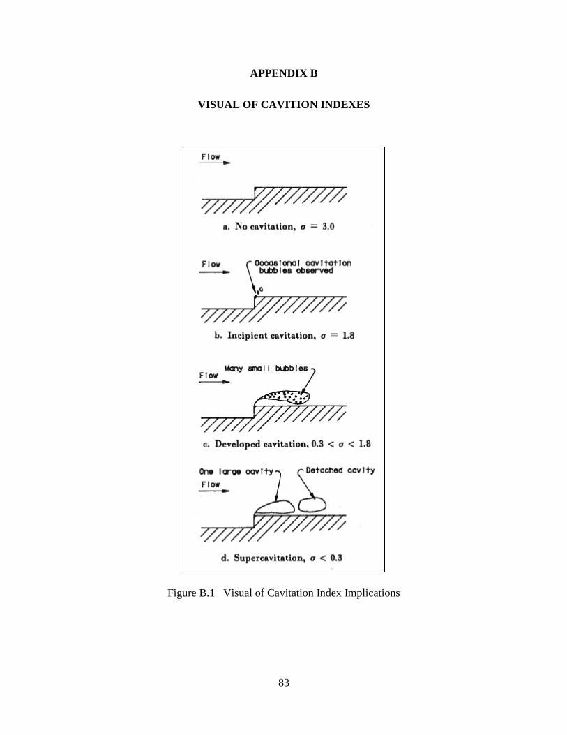
83
APPENDIX B
VISUAL OF CAVITION INDEXES
Figure B.1 Visual of Cavitation Index Implications
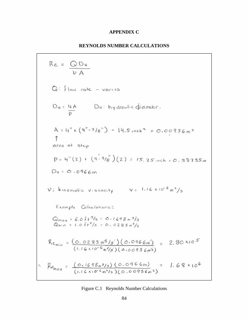
84
APPENDIX C
REYNOLDS NUMBER CALCULATIONS
Figure C.1 Reynolds Number Calculations
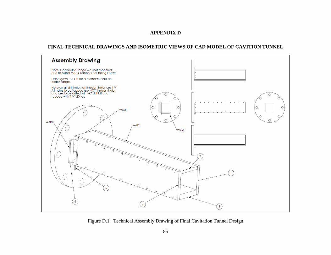
85
APPENDIX D
FINAL TECHNICAL DRAWINGS AND ISOMETRIC VIEWS OF CAD MODEL OF CAVITION TUNNEL
Figure D.1 Technical Assembly Drawing of Final Cavitation Tunnel Design
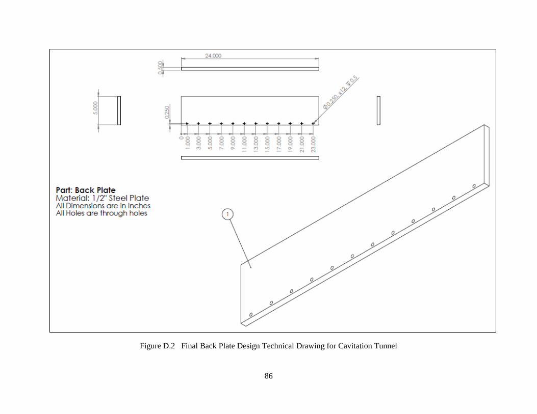
86
Figure D.2 Final Back Plate Design Technical Drawing for Cavitation Tunnel
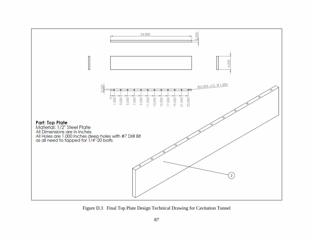
87
Figure D.3 Final Top Plate Design Technical Drawing for Cavitation Tunnel
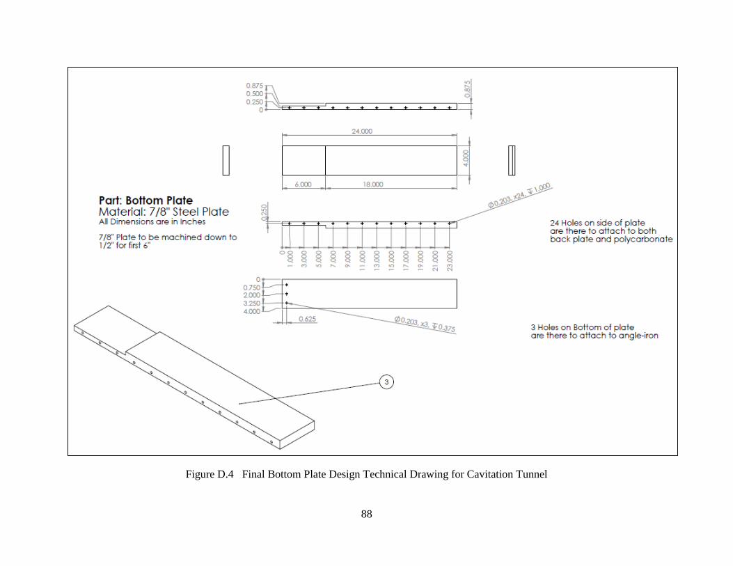
88
Figure D.4 Final Bottom Plate Design Technical Drawing for Cavitation Tunnel
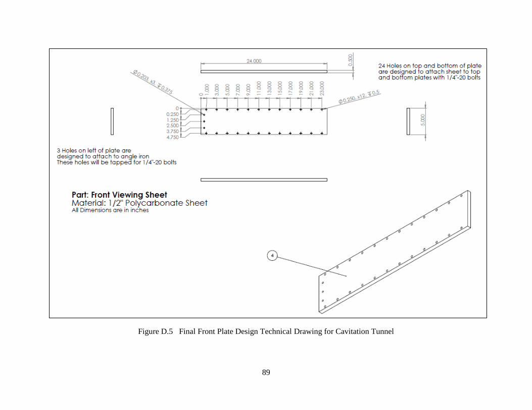
89
Figure D.5 Final Front Plate Design Technical Drawing for Cavitation Tunnel
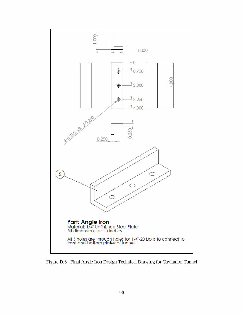
90
Figure D.6 Final Angle Iron Design Technical Drawing for Cavitation Tunnel
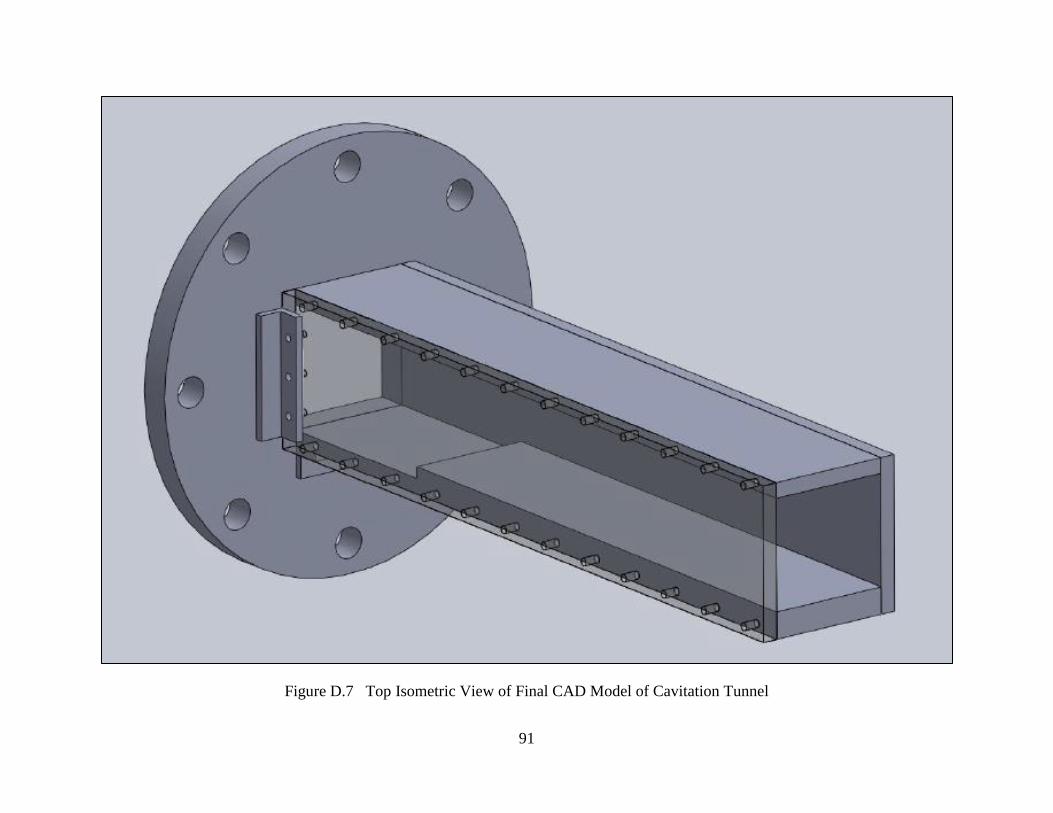
91
Figure D.7 Top Isometric View of Final CAD Model of Cavitation Tunnel
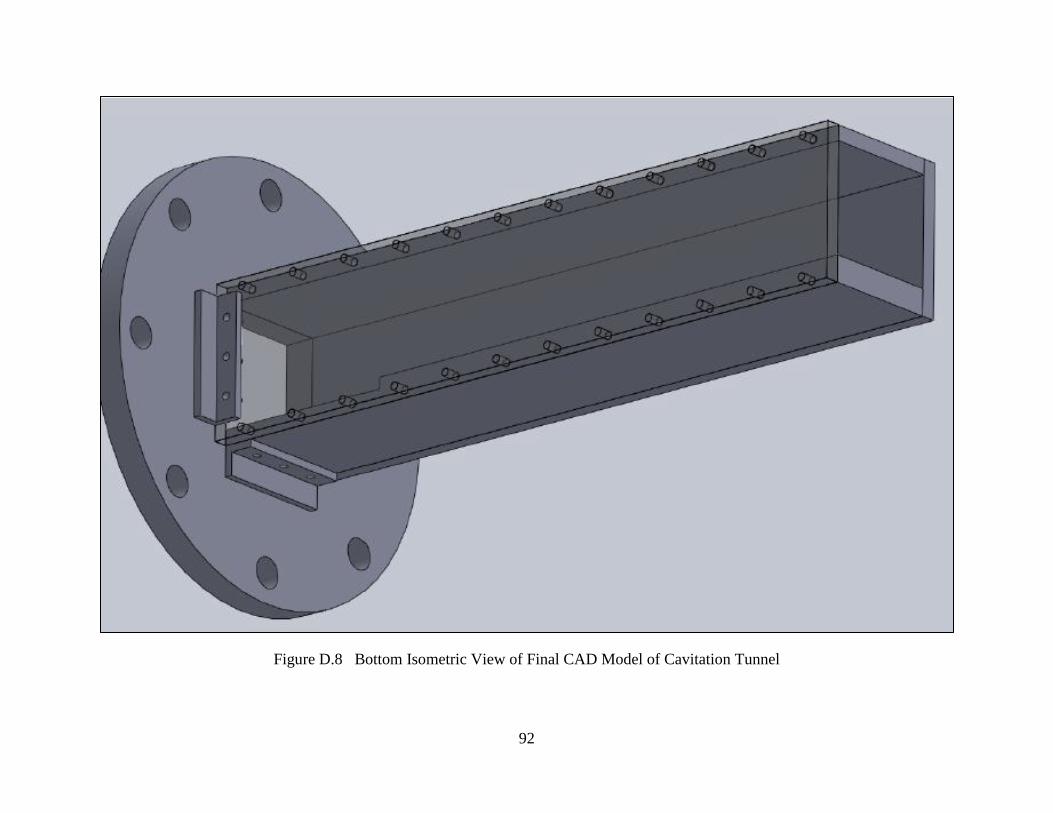
92
Figure D.8 Bottom Isometric View of Final CAD Model of Cavitation Tunnel
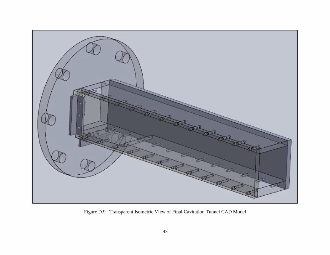
93
Figure D.9 Transparent Isometric View of Final Cavitation Tunnel CAD Model
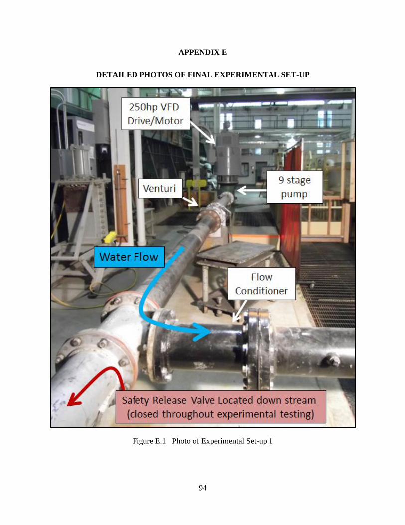
94
APPENDIX E
DETAILED PHOTOS OF FINAL EXPERIMENTAL SET-UP
Figure E.1 Photo of Experimental Set-up 1
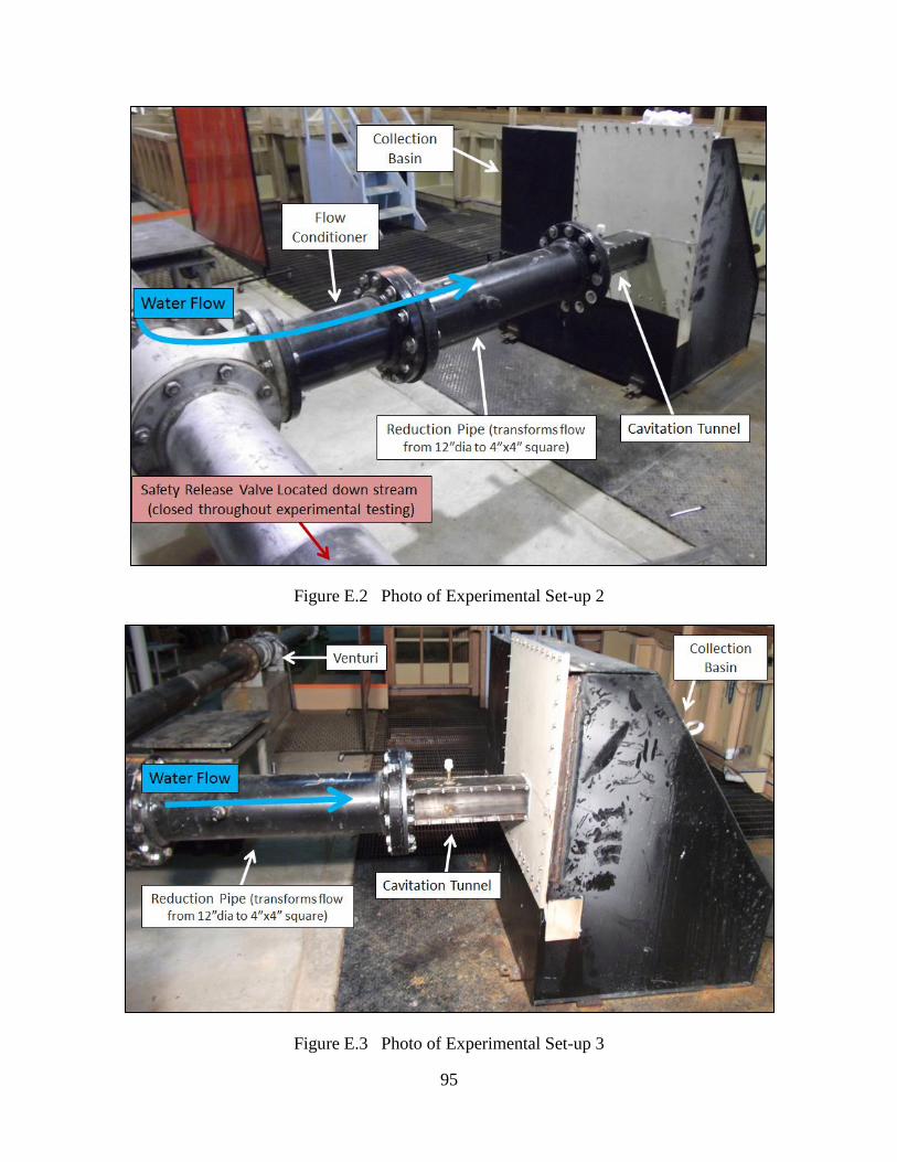
95
Figure E.2 Photo of Experimental Set-up 2
Figure E.3 Photo of Experimental Set-up 3
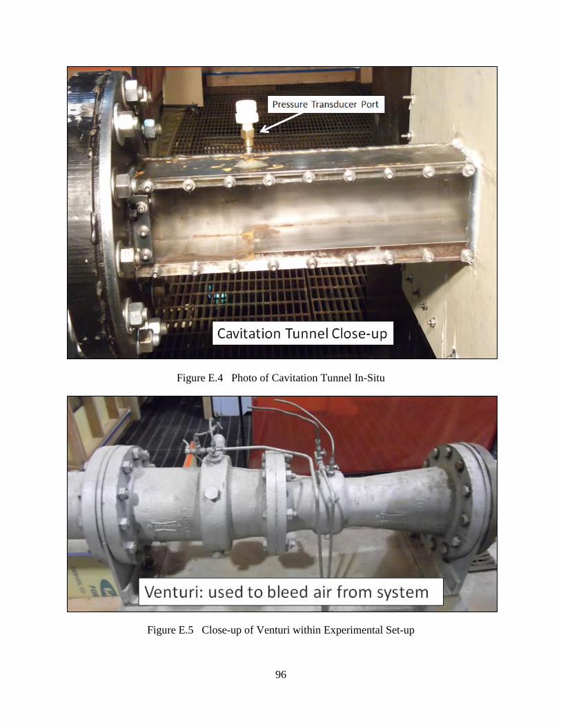
96
Figure E.4 Photo of Cavitation Tunnel In-Situ
Figure E.5 Close-up of Venturi within Experimental Set-up
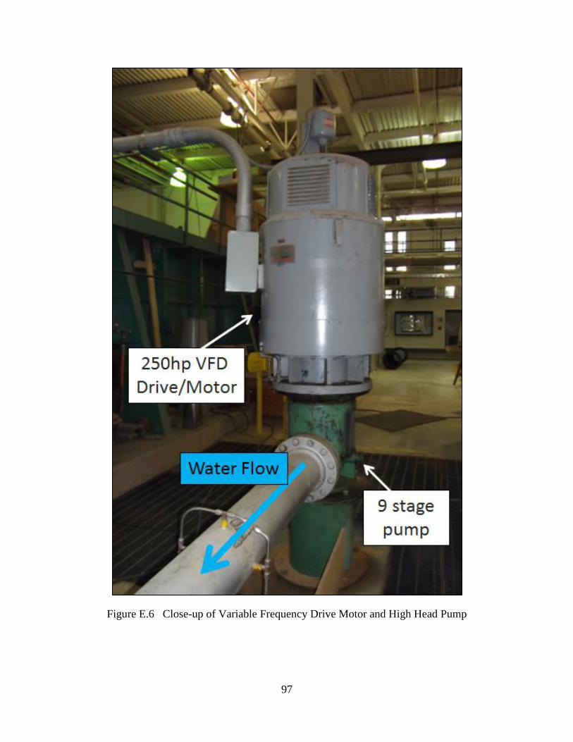
97
Figure E.6 Close-up of Variable Frequency Drive Motor and High Head Pump
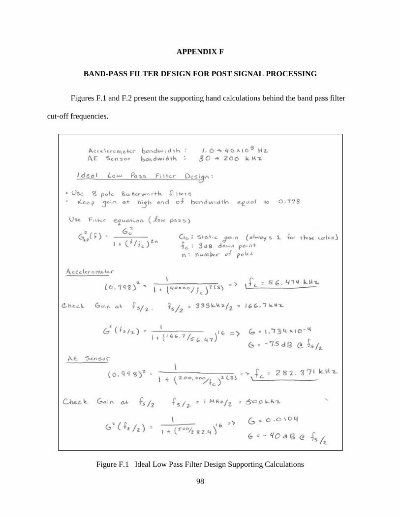
98
APPENDIX F
BAND-PASS FILTER DESIGN FOR POST SIGNAL PROCESSING
Figures F.1 and F.2 present the supporting hand calculations behind the band pass filter
cut-off frequencies.
Figure F.1 Ideal Low Pass Filter Design Supporting Calculations
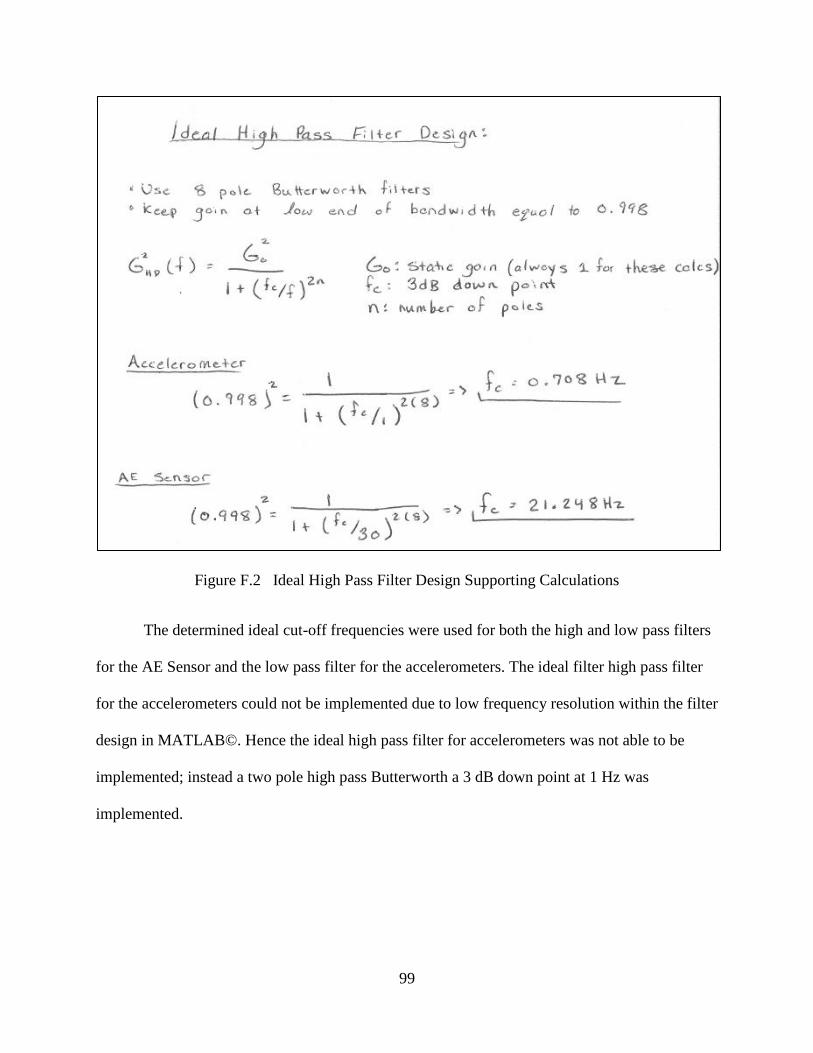
99
Figure F.2 Ideal High Pass Filter Design Supporting Calculations
The determined ideal cut-off frequencies were used for both the high and low pass filters
for the AE Sensor and the low pass filter for the accelerometers. The ideal filter high pass filter
for the accelerometers could not be implemented due to low frequency resolution within the filter
design in MATLAB©. Hence the ideal high pass filter for accelerometers was not able to be
implemented; instead a two pole high pass Butterworth a 3 dB down point at 1 Hz was
implemented.
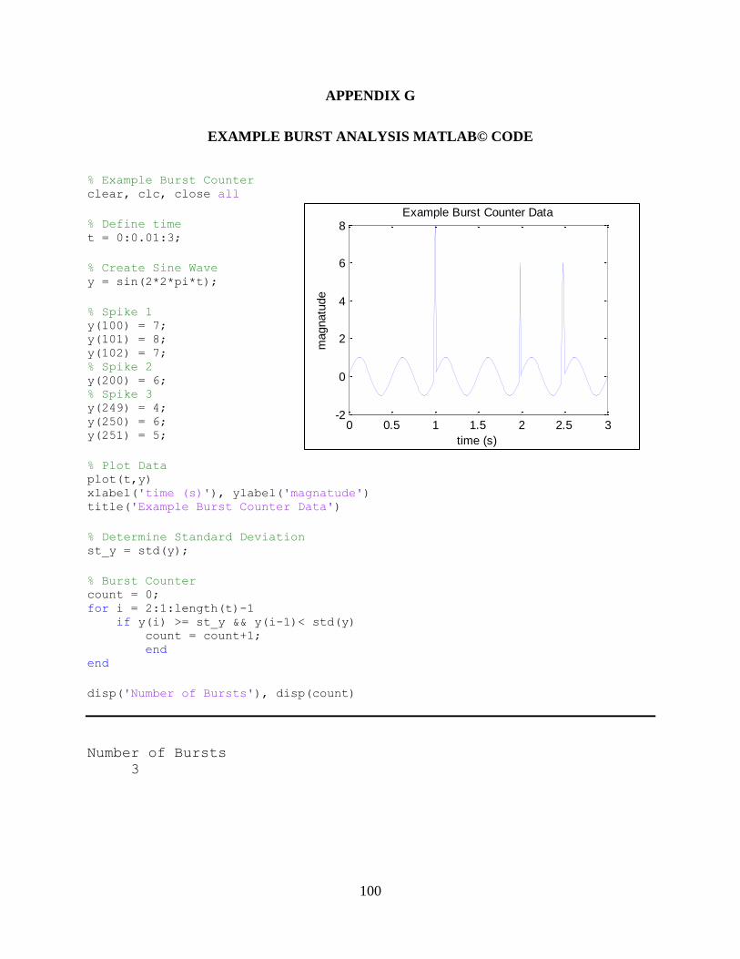
100
0 0.5 1 1.5 2 2.5 3-2
0
2
4
6
8
time (s)
magnatu
de
Example Burst Counter Data
APPENDIX G
EXAMPLE BURST ANALYSIS MATLAB© CODE
% Example Burst Counter clear, clc, close all
% Define time t = 0:0.01:3;
% Create Sine Wave y = sin(2*2*pi*t);
% Spike 1 y(100) = 7; y(101) = 8; y(102) = 7; % Spike 2 y(200) = 6; % Spike 3 y(249) = 4; y(250) = 6; y(251) = 5;
% Plot Data plot(t,y) xlabel('time (s)'), ylabel('magnatude') title('Example Burst Counter Data')
% Determine Standard Deviation st_y = std(y);
% Burst Counter count = 0; for i = 2:1:length(t)-1 if y(i) >= st_y && y(i-1)< std(y) count = count+1; end end
disp('Number of Bursts'), disp(count)
Number of Bursts
3
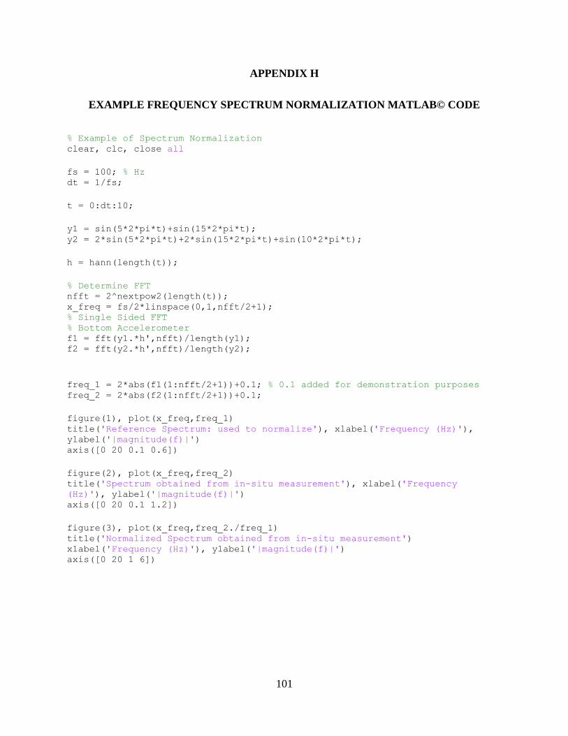
101
APPENDIX H
EXAMPLE FREQUENCY SPECTRUM NORMALIZATION MATLAB© CODE
% Example of Spectrum Normalization clear, clc, close all
fs = 100; % Hz dt = 1/fs;
t = 0:dt:10;
y1 = sin(5*2*pi*t)+sin(15*2*pi*t); y2 = 2*sin(5*2*pi*t)+2*sin(15*2*pi*t)+sin(10*2*pi*t);
h = hann(length(t));
% Determine FFT nfft = 2^nextpow2(length(t)); x_freq = fs/2*linspace(0,1,nfft/2+1); % Single Sided FFT % Bottom Accelerometer f1 = fft(y1.*h',nfft)/length(y1); f2 = fft(y2.*h',nfft)/length(y2);
freq_1 = 2*abs(f1(1:nfft/2+1))+0.1; % 0.1 added for demonstration purposes freq_2 = 2*abs(f2(1:nfft/2+1))+0.1;
figure(1), plot(x_freq,freq_1) title('Reference Spectrum: used to normalize'), xlabel('Frequency (Hz)'),
ylabel('|magnitude(f)|') axis([0 20 0.1 0.6])
figure(2), plot(x_freq,freq_2) title('Spectrum obtained from in-situ measurement'), xlabel('Frequency
(Hz)'), ylabel('|magnitude(f)|') axis([0 20 0.1 1.2])
figure(3), plot(x_freq,freq_2./freq_1) title('Normalized Spectrum obtained from in-situ measurement') xlabel('Frequency (Hz)'), ylabel('|magnitude(f)|') axis([0 20 1 6])
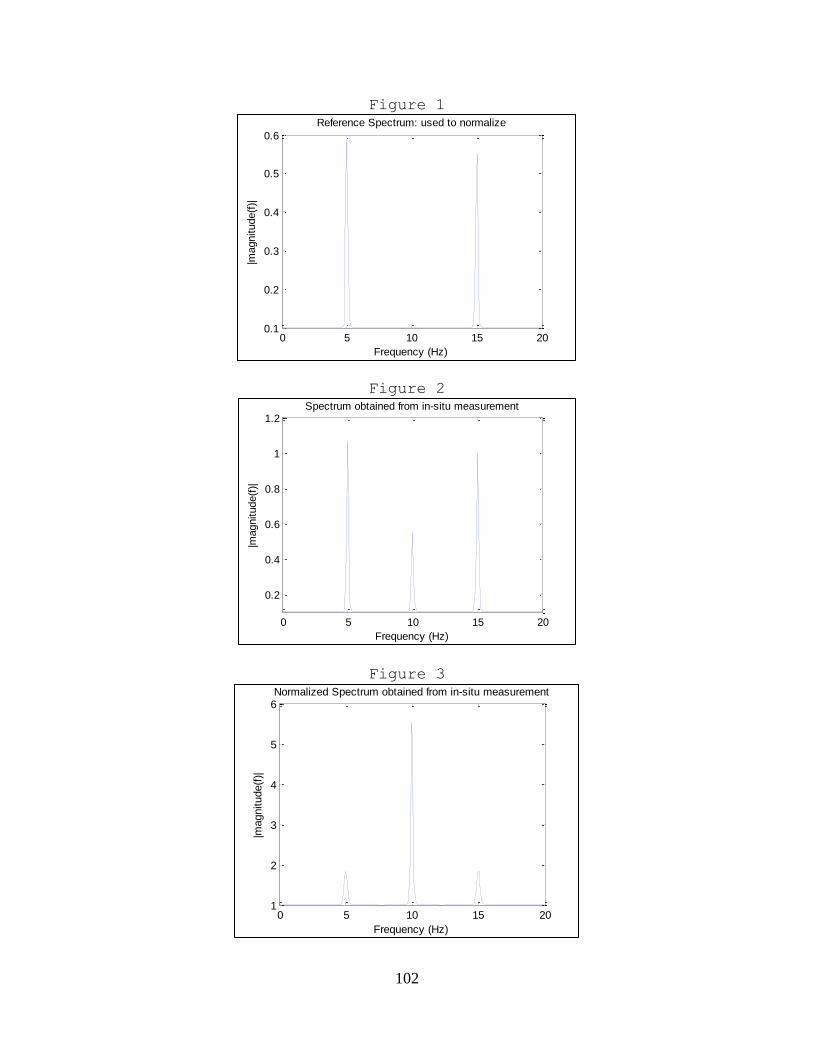
102
Figure 1
Figure 2
Figure 3
0 5 10 15 200.1
0.2
0.3
0.4
0.5
0.6
Reference Spectrum: used to normalize
Frequency (Hz)
|magnitude(f
)|
0 5 10 15 20
0.2
0.4
0.6
0.8
1
1.2Spectrum obtained from in-situ measurement
Frequency (Hz)
|magnitude(f
)|
0 5 10 15 201
2
3
4
5
6Normalized Spectrum obtained from in-situ measurement
Frequency (Hz)
|magnitude(f
)|
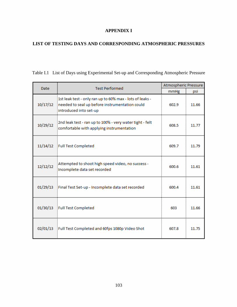
103
APPENDIX I
LIST OF TESTING DAYS AND CORRESPONDING ATMOSPHERIC PRESSURES
Table I.1 List of Days using Experimental Set-up and Corresponding Atmospheric Pressure
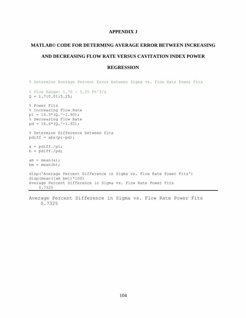
104
APPENDIX J
MATLAB© CODE FOR DETERMING AVERAGE ERROR BETWEEN INCREASING
AND DECREASING FLOW RATE VERSUS CAVITATION INDEX POWER
REGRESSION
% Determine Average Percent Error between Sigma vs. Flow Rate Power Fits
% Flow Range: 1.70 - 5.25 ft^3/s Q = 1.7:0.01:5.25;
% Power Fits
% Increasing Flow Rate
pi = 16.3*(Q.^-1.90);
% Decreasing Flow Rate
pd = 16.6*(Q.^-1.92);
% Determine Difference between fits
pdiff = abs(pi-pd);
a = pdiff./pi;
b = pdiff./pd;
am = mean(a);
bm = mean(b);
disp('Average Percent Difference in Sigma vs. Flow Rate Power Fits')
disp(mean([am bm])*100)
Average Percent Difference in Sigma vs. Flow Rate Power Fits
0.7325
Average Percent Difference in Sigma vs. Flow Rate Power Fits
0.7325
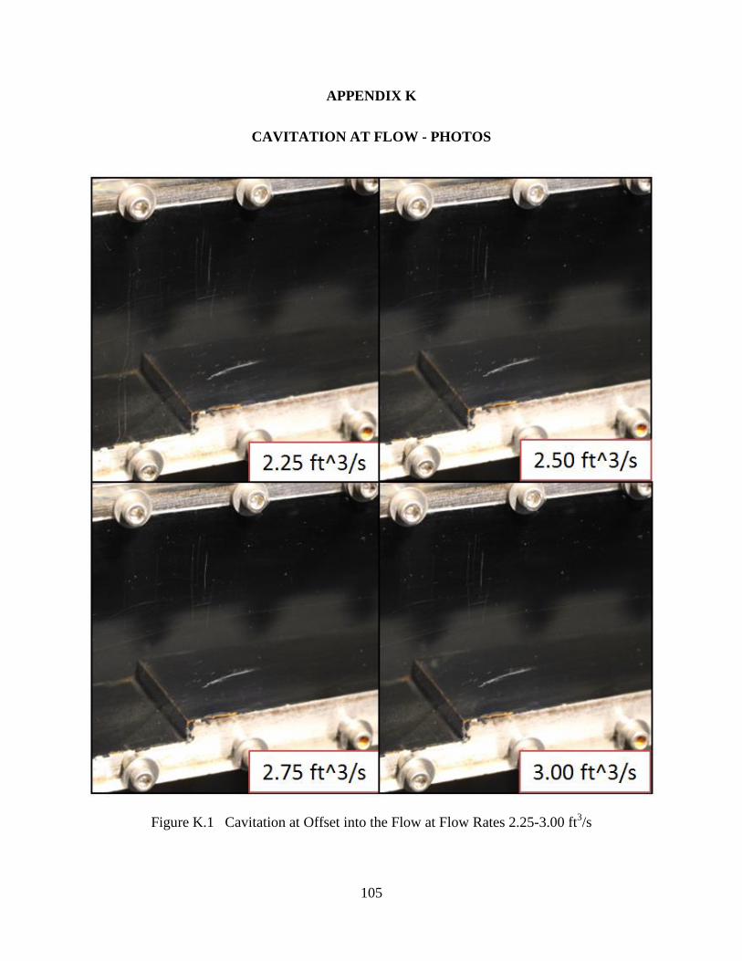
105
APPENDIX K
CAVITATION AT FLOW - PHOTOS
Figure K.1 Cavitation at Offset into the Flow at Flow Rates 2.25-3.00 ft3/s
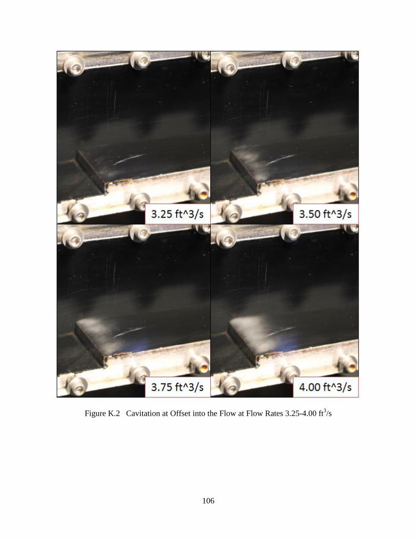
106
Figure K.2 Cavitation at Offset into the Flow at Flow Rates 3.25-4.00 ft3/s
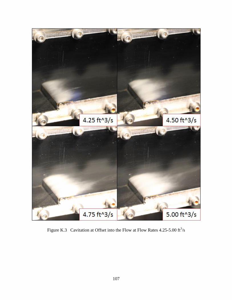
107
Figure K.3 Cavitation at Offset into the Flow at Flow Rates 4.25-5.00 ft3/s
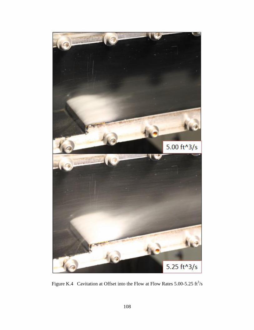
108
Figure K.4 Cavitation at Offset into the Flow at Flow Rates 5.00-5.25 ft3/s
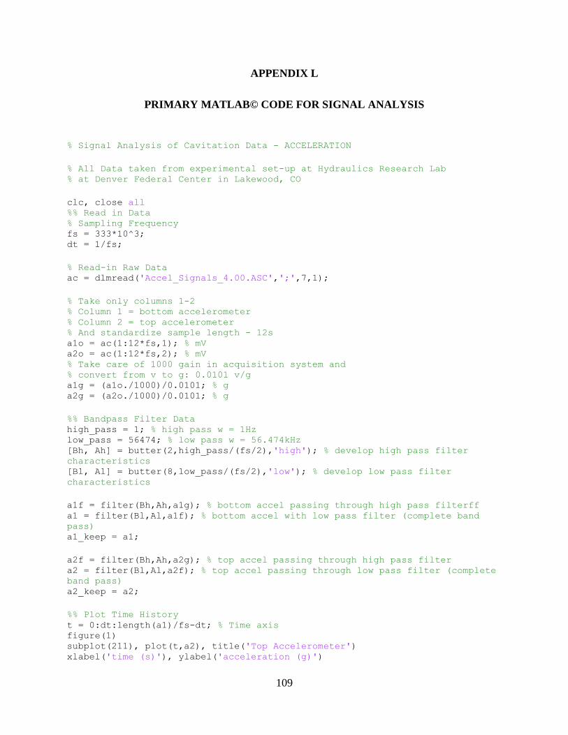
109
APPENDIX L
PRIMARY MATLAB© CODE FOR SIGNAL ANALYSIS
% Signal Analysis of Cavitation Data - ACCELERATION
% All Data taken from experimental set-up at Hydraulics Research Lab % at Denver Federal Center in Lakewood, CO
clc, close all %% Read in Data % Sampling Frequency fs = 333*10^3; dt = 1/fs;
% Read-in Raw Data ac = dlmread('Accel_Signals_4.00.ASC',';',7,1);
% Take only columns 1-2 % Column 1 = bottom accelerometer % Column 2 = top accelerometer % And standardize sample length - 12s a1o = ac(1:12*fs,1); % mV a2o = ac(1:12*fs,2); % mV % Take care of 1000 gain in acquisition system and % convert from v to g: 0.0101 v/g a1g = (a1o./1000)/0.0101; % g a2g = (a2o./1000)/0.0101; % g
%% Bandpass Filter Data high_pass = 1; % high pass w = 1Hz low_pass = 56474; % low pass w = 56.474kHz [Bh, Ah] = butter(2,high_pass/(fs/2),'high'); % develop high pass filter
characteristics [Bl, Al] = butter(8,low_pass/(fs/2),'low'); % develop low pass filter
characteristics
a1f = filter(Bh,Ah,a1g); % bottom accel passing through high pass filterff a1 = filter(Bl,Al,a1f); % bottom accel with low pass filter (complete band
pass) a1_keep = a1;
a2f = filter(Bh,Ah,a2g); % top accel passing through high pass filter a2 = filter(Bl,Al,a2f); % top accel passing through low pass filter (complete
band pass) a2_keep = a2;
%% Plot Time History t = 0:dt:length(a1)/fs-dt; % Time axis figure(1) subplot(211), plot(t,a2), title('Top Accelerometer') xlabel('time (s)'), ylabel('acceleration (g)')
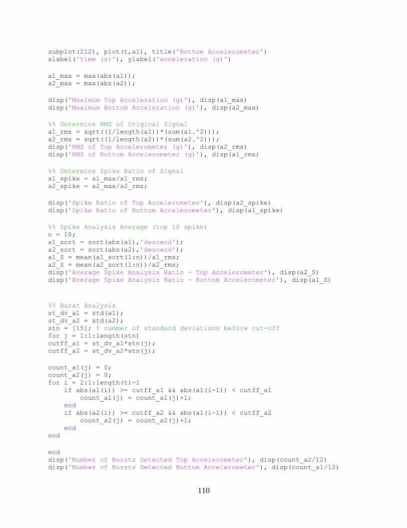
110
subplot(212), plot(t,a1), title('Bottom Accelerometer') xlabel('time (s)'), ylabel('acceleration (g)')
a1_max = max(abs(a1)); a2_max = max(abs(a2));
disp('Maximum Top Acceleration (g)'), disp(a1_max) disp('Maximum Bottom Acceleration (g)'), disp(a2_max)
%% Determine RMS of Original Signal a1_rms = sqrt((1/length(a1))*(sum(a1.^2))); a2_rms = sqrt((1/length(a2))*(sum(a2.^2))); disp('RMS of Top Accelerometer (g)'), disp(a2_rms) disp('RMS of Bottom Accelerometer (g)'), disp(a1_rms)
%% Determine Spike Ratio of Signal a1_spike = a1_max/a1_rms; a2_spike = a2_max/a2_rms;
disp('Spike Ratio of Top Accelerometer'), disp(a2_spike) disp('Spike Ratio of Bottom Accelerometer'), disp(a1_spike)
%% Spike Analysis Average (top 10 spike) n = 10; a1_sort = sort(abs(a1),'descend'); a2_sort = sort(abs(a2),'descend'); a1_S = mean(a1_sort(1:n))/a1_rms; a2_S = mean(a2_sort(1:n))/a2_rms; disp('Average Spike Analysis Ratio - Top Accelerometer'), disp(a2_S) disp('Average Spike Analysis Ratio - Bottom Accelerometer'), disp(a1_S)
%% Burst Analysis st_dv_a1 = std(a1); st_dv_a2 = std(a2); stn = [15]; % number of standard deviations before cut-off for j = 1:1:length(stn) cutff_a1 = st_dv_a1*stn(j); cutff_a2 = st_dv_a2*stn(j);
count_a1(j) = 0; count_a2(j) = 0; for i = 2:1:length(t)-1 if abs(a1(i)) >= cutff_a1 && abs(a1(i-1)) < cutff_a1 count_a1(j) = count_a1(j)+1; end if abs(a2(i)) >= cutff_a2 && abs(a1(i-1)) < cutff_a2 count_a2(j) = count_a2(j)+1; end end
end disp('Number of Bursts Detected Top Accelerometer'), disp(count_a2/12) disp('Number of Bursts Detected Bottom Accelerometer'), disp(count_a1/12)
111
%% Determine Auto-Correlation of signals % Auto Correlation of Bottom Accelerometer X_1 = xcorr(a1,a1); % Auto Correlation of Top Accelerometer X_2 = xcorr(a2,a2);
figure(2) subplot(211), plot((X_2./(max(X_2)))*100), title('Auto-Correlation of Top
Accelerometer') ylabel('Percent Correlation (%)') subplot(212), plot((X_1./(max(X_1)))*100), title('Auto-Correlation of Bottom
Accelerometer') ylabel('Percent Correlation (%)') % %% Apply Hanning Window Prior to Further Analysis whann = hann(length(t)); a1 = a1.*whann; a2 = a2.*whann;
%% Determine FFT of Signals nfft = 2^nextpow2(length(t)); x_freq = fs/2*linspace(0,1,nfft/2+1); % Single Sided FFT % Bottom Accelerometer y1 = fft(a1,nfft)/length(a1); freq_1 = 2*abs(y1(1:nfft/2+1)); % Top Accelerometer y2 = fft(a2,nfft)/length(a2); freq_2 = 2*abs(y2(1:nfft/2+1));
y_max_1 = max(freq_1(250:length(freq_1))); y_max_2 = max(freq_2(250:length(freq_2))); y_max =(max([y_max_1 y_max_2])); figure(3) subplot(211), plot(x_freq,freq_2), title('FFT of Top Accelerometer') xlabel('Frequency (Hz)'), ylabel('|g(f)|'), axis([high_pass low_pass 0
y_max*1.025]), % axis 'auto y' subplot(212), plot(x_freq,freq_1), title('FFT of Bottom Accelerometer') xlabel('Frequency (Hz)'), ylabel('|g(f)|'), axis([high_pass low_pass 0
y_max*1.025]), % axis 'auto y'
for i = 1:1:length(x_freq) if freq_1(i) == y_max_1 freq_c_1 = x_freq(i); end if freq_2(i) == y_max_2 freq_c_2 = x_freq(i); end end
disp('Maximum Top Acceleration in Frequency domain - max|g(f)|'),
disp(y_max_2) disp('Maximum Top Acceleration Corresponding Frequency (Hz)'), disp(freq_c_2) disp('Maximum Bottom Acceleration in Frequency domain - max|g(f)|'),
disp(y_max_1)
112
disp('Maximum Bottom Acceleration Corresponding Frequency (Hz)'),
disp(freq_c_1)
%% Normalized FFT load FFT_Spectrum_Normalization_Accels % normalized with original averaged FFT freq1_n = freq_1./B_FFT_norm'; freq2_n = freq_2./T_FFT_norm'; % normalized with 1Hz average FFT freq1_n1 = freq_1./B_FFT_norm_1; freq2_n1 = freq_2./T_FFT_norm_1; % normalized with 1Hz average FFT freq1_n2 = freq_1./B_FFT_norm_2; freq2_n2 = freq_2./T_FFT_norm_2; % normalized with 1Hz average FFT freq1_n5 = freq_1./B_FFT_norm_5; freq2_n5 = freq_2./T_FFT_norm_5; figure(4) subplot(211), plot(x_freq,freq_2_norm), title('Normalized FFT of Top
Accelerometer') xlabel('Frequency (Hz)'), ylabel('|g(f)| - normalized'), axis([0 40000 0 1]),
axis 'auto y' subplot(212), plot(x_freq,freq_1_norm), title('Normalized FFT of Bottom
Accelerometer') xlabel('Frequency (Hz)'), ylabel('|g(f)|-normalized'), axis([0 40000 0 1]),
axis 'auto y'
%% Determine Power Spectral Density (PSD) % Bottom Accelerometer PSD Pxx_1 = abs(fft(a1,nfft)).^2/length(a1)/fs; Hpsd_1 = dspdata.psd(Pxx_1(1:length(Pxx_1)/2),'Fs',fs); % Top Accelerometer PSD Pxx_2 = abs(fft(a2,nfft)).^2/length(a2)/fs; Hpsd_2 = dspdata.psd(Pxx_2(1:length(Pxx_2)/2),'Fs',fs);
figure(5) subplot(211), plot(Hpsd_2), title('PSD of Top Accelerometer') axis([0 40000 -100 100]), axis 'auto y' subplot(212), plot(Hpsd_1), title('PSD of Bottom Accelerometer') axis([0 40000 -100 100]), axis 'auto y'
%% Determine Coherence of Signals % size of Hanning window (power to be applied to 2) h = 15; [Cxy,W] = mscohere(a1_keep,a2_keep,hanning(2^h),2^(h-1),nfft); figure(5), plot(x_freq,Cxy), title('Coherence of Top and Bottom
Accelerometers') xlabel('Frequency (Hz)'), ylabel('Coherence'), axis([0 40000 0 1])
113
% Signal Analysis of Cavitation Data - ACOUSTIC EMISSION
% All Data taken from experimental set-up at Hydraulics Research Lab % at Denver Federal Center in Lakewood, CO
clc, clear, close all %% Read in Data % Sampling Frequency fs = 1*10^6; dt = 1/fs;
% Read-in Raw Data aer = dlmread('AE_Signal_4.00.ASC',';',7,1); % Raw Data - V aeo = aer(1:8.5*fs,1); % Remove extra column of zeros and only take 1st 8.5s % Reduce Data - due to 40db (100x) gain on instrumentation aeg = (aeo/100)*1000; % mv
%% Bandpass Filter Data high_pass = 21249; % high pass w = 30kHz low_pass = 282371; % low pass w = 200kHz [Bh, Ah] = butter(8,high_pass/(fs/2),'high'); % develop high pass filter
characteristics [Bl, Al] = butter(8,low_pass/(fs/2),'low'); % develop low pass filter
characteristics
aef = filter(Bh,Ah,aeg); % Acoustic Emission high pass filter ae = filter(Bl,Al,aef); % Acoustic Emission low pass filter (complete band
pass)
%% Plot Time History t = 0:dt:length(ae)/fs-dt; % Time axis figure(1) plot(t,ae), title('Acoustic Emission') xlabel('time (s)'), ylabel('Voltage output (mV)')
ae_max = max(abs(ae)); disp('Maximum AE Reading (mV)'), disp(ae_max)
%% Determine RMS of Signals ae_rms = sqrt((1/length(ae))*(sum(ae.^2))); disp('RMS of AE Sensor (mV)'), disp(ae_rms)
%% Determine Spike Ratio of Signal ae_spike = ae_max/ae_rms;
disp('Spike Ratio of AE Sensor'), disp(ae_spike)
%% Spike Analysis Average (top 10 spike) n = 10; ae_sort = sort(abs(ae),'descend'); ae_S = mean(ae_sort(1:n))/ae_rms; disp('Average Spike Analysis Ratio - AE Sensor'), disp(ae_S)
114
%% Burst Analysis st_dv_ae = std(ae);
stn = [5]; % number of standard deviations before cut-off for j = 1:1:length(stn) cutff_ae = st_dv_ae*stn(j);
count_ae(j) = 0;
for i = 2:1:length(t)-1 if abs(ae(i)) >= cutff_ae && abs(ae(i-1)) < cutff_ae count_ae(j)= count_ae(j)+1; end end
end
disp('Number of Bursts Detected Per Second - AE Sensor'), disp(count_ae/8.5)
%% Determine Auto-Correlation of signals % Auto Correlation of AE Sensor X = xcorr(ae,ae); figure(2) plot((X./(max(X)))*100), title('Auto-Correlation AE Sensor') ylabel('Percent Correlation (%)')
%% Apply Hanning Window Prior to Further Analysis whann = hann(length(t)); ae = ae.*whann;
%% Determine FFT of Signals nfft = 2^nextpow2(length(t)); x_freq = fs/2*linspace(0,1,nfft/2+1); % Single Sided FFT y = fft(ae,nfft)/length(ae); freq = 2*abs(y(1:nfft/2+1));
y_max = max(freq); figure(3) plot(x_freq,freq), title('FFT of AE Sensor') xlabel('Frequency (Hz)'), ylabel('|mV(f)|'), axis([high_pass low_pass 0 1]),
axis 'auto y'
for i = 1:1:length(x_freq) if freq(i) == y_max freq_c = x_freq(i); end end
disp('Maximum Top Acceleration in Frequency domain - max|g(f)|'), disp(y_max) disp('Maximum Top Acceleration Corresponding Frequency (Hz)'), disp(freq_c)
%% Normalized FFT
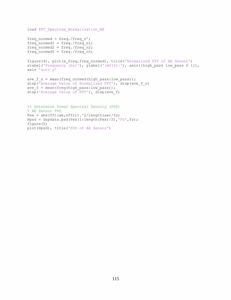
115
load FFT_Spectrum_Normalization_AE
freq_normed = freq./freq_n'; freq_normed1 = freq./freq_n1; freq_normed2 = freq./freq_n2; freq_normed5 = freq./freq_n5;
figure(4), plot(x_freq,freq_normed), title('Normalized FFT of AE Sensor') xlabel('Frequency (Hz)'), ylabel('|mV(f)|'), axis([high_pass low_pass 0 1]),
axis 'auto y'
ave_f_n = mean(freq_normed(high_pass:low_pass)); disp('Average Value of Normalized FFT'), disp(ave_f_n) ave_f = mean(freq(high_pass:low_pass)); disp('Average Value of FFT'), disp(ave_f)
%% Determine Power Spectral Density (PSD) % AE Sensor PSD Pxx = abs(fft(ae,nfft)).^2/length(ae)/fs; Hpsd = dspdata.psd(Pxx(1:length(Pxx)/2),'Fs',fs); figure(5) plot(Hpsd), title('PSD of AE Sensor')
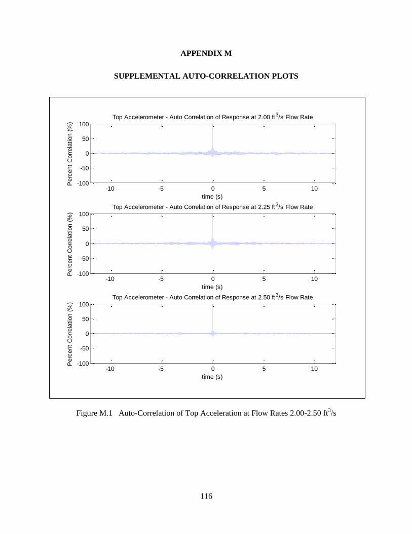
116
APPENDIX M
SUPPLEMENTAL AUTO-CORRELATION PLOTS
Figure M.1 Auto-Correlation of Top Acceleration at Flow Rates 2.00-2.50 ft3/s
-10 -5 0 5 10-100
-50
0
50
100Top Accelerometer - Auto Correlation of Response at 2.00 ft3/s Flow Rate
Perc
ent
Corr
ela
tion (
%)
time (s)
-10 -5 0 5 10-100
-50
0
50
100Top Accelerometer - Auto Correlation of Response at 2.25 ft3/s Flow Rate
Perc
ent
Corr
ela
tion (
%)
time (s)
-10 -5 0 5 10-100
-50
0
50
100Top Accelerometer - Auto Correlation of Response at 2.50 ft3/s Flow Rate
Perc
ent
Corr
ela
tion (
%)
time (s)
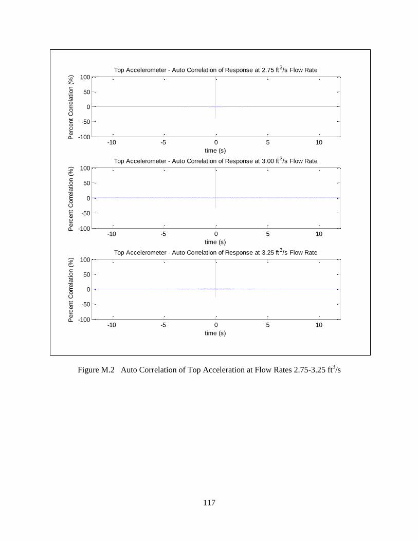
117
Figure M.2 Auto Correlation of Top Acceleration at Flow Rates 2.75-3.25 ft3/s
-10 -5 0 5 10-100
-50
0
50
100Top Accelerometer - Auto Correlation of Response at 2.75 ft3/s Flow Rate
Perc
ent
Corr
ela
tion (
%)
time (s)
-10 -5 0 5 10-100
-50
0
50
100Top Accelerometer - Auto Correlation of Response at 3.00 ft3/s Flow Rate
Perc
ent
Corr
ela
tion (
%)
time (s)
-10 -5 0 5 10-100
-50
0
50
100Top Accelerometer - Auto Correlation of Response at 3.25 ft3/s Flow Rate
Perc
ent
Corr
ela
tion (
%)
time (s)
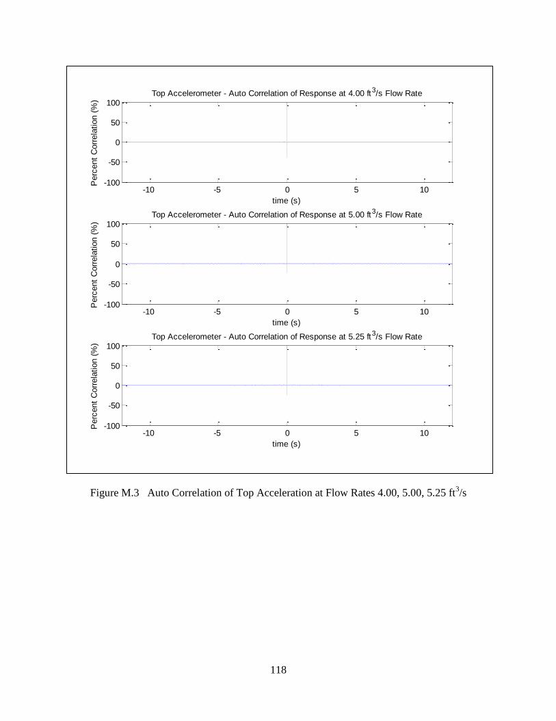
118
Figure M.3 Auto Correlation of Top Acceleration at Flow Rates 4.00, 5.00, 5.25 ft3/s
-10 -5 0 5 10-100
-50
0
50
100Top Accelerometer - Auto Correlation of Response at 4.00 ft3/s Flow Rate
Perc
ent
Corr
ela
tion (
%)
time (s)
-10 -5 0 5 10-100
-50
0
50
100Top Accelerometer - Auto Correlation of Response at 5.00 ft3/s Flow Rate
Perc
ent
Corr
ela
tion (
%)
time (s)
-10 -5 0 5 10-100
-50
0
50
100Top Accelerometer - Auto Correlation of Response at 5.25 ft3/s Flow Rate
Perc
ent
Corr
ela
tion (
%)
time (s)
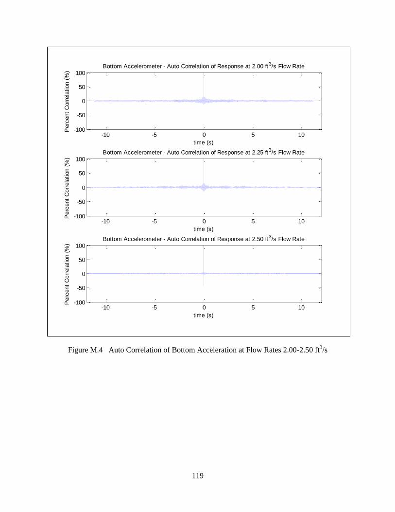
119
Figure M.4 Auto Correlation of Bottom Acceleration at Flow Rates 2.00-2.50 ft3/s
-10 -5 0 5 10-100
-50
0
50
100Bottom Accelerometer - Auto Correlation of Response at 2.00 ft3/s Flow Rate
Perc
ent
Corr
ela
tion (
%)
time (s)
-10 -5 0 5 10-100
-50
0
50
100Bottom Accelerometer - Auto Correlation of Response at 2.25 ft3/s Flow Rate
Perc
ent
Corr
ela
tion (
%)
time (s)
-10 -5 0 5 10-100
-50
0
50
100Bottom Accelerometer - Auto Correlation of Response at 2.50 ft3/s Flow Rate
Perc
ent
Corr
ela
tion (
%)
time (s)
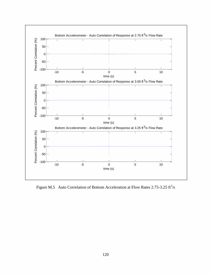
120
Figure M.5 Auto Correlation of Bottom Acceleration at Flow Rates 2.75-3.25 ft3/s
-10 -5 0 5 10-100
-50
0
50
100Bottom Accelerometer - Auto Correlation of Response at 2.75 ft3/s Flow Rate
Perc
ent
Corr
ela
tion (
%)
time (s)
-10 -5 0 5 10-100
-50
0
50
100Bottom Accelerometer - Auto Correlation of Response at 3.00 ft3/s Flow Rate
Perc
ent
Corr
ela
tion (
%)
time (s)
-10 -5 0 5 10-100
-50
0
50
100Bottom Accelerometer - Auto Correlation of Response at 3.25 ft3/s Flow Rate
Perc
ent
Corr
ela
tion (
%)
time (s)

121
Figure M.6 Auto Correlation of Bottom Acceleration at Flow Rates 4.00, 5.00, 5.25 ft3/s
-10 -5 0 5 10-100
-50
0
50
100Bottom Accelerometer - Auto Correlation of Response at 4.00 ft3/s Flow Rate
Perc
ent
Corr
ela
tion (
%)
time (s)
-10 -5 0 5 10-100
-50
0
50
100Bottom Accelerometer - Auto Correlation of Response at 5.00 ft3/s Flow Rate
Perc
ent
Corr
ela
tion (
%)
time (s)
-10 -5 0 5 10-100
-50
0
50
100Bottom Accelerometer - Auto Correlation of Response at 5.25 ft3/s Flow Rate
Perc
ent
Corr
ela
tion (
%)
time (s)
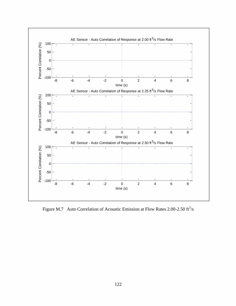
122
Figure M.7 Auto Correlation of Acoustic Emission at Flow Rates 2.00-2.50 ft3/s
-8 -6 -4 -2 0 2 4 6 8-100
-50
0
50
100AE Sensor - Auto Correlation of Response at 2.00 ft3/s Flow Rate
Perc
ent
Corr
ela
tion (
%)
time (s)
-8 -6 -4 -2 0 2 4 6 8-100
-50
0
50
100AE Sensor - Auto Correlation of Response at 2.25 ft3/s Flow Rate
Perc
ent
Corr
ela
tion (
%)
time (s)
-8 -6 -4 -2 0 2 4 6 8-100
-50
0
50
100AE Sensor - Auto Correlation of Response at 2.50 ft3/s Flow Rate
Perc
ent
Corr
ela
tion (
%)
time (s)
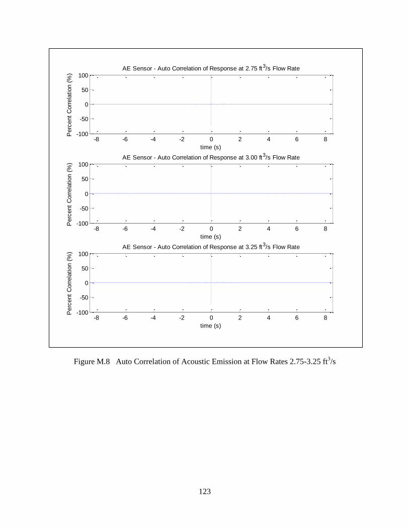
123
Figure M.8 Auto Correlation of Acoustic Emission at Flow Rates 2.75-3.25 ft3/s
-8 -6 -4 -2 0 2 4 6 8-100
-50
0
50
100AE Sensor - Auto Correlation of Response at 2.75 ft3/s Flow Rate
Perc
ent
Corr
ela
tion (
%)
time (s)
-8 -6 -4 -2 0 2 4 6 8-100
-50
0
50
100AE Sensor - Auto Correlation of Response at 3.00 ft3/s Flow Rate
Perc
ent
Corr
ela
tion (
%)
time (s)
-8 -6 -4 -2 0 2 4 6 8-100
-50
0
50
100AE Sensor - Auto Correlation of Response at 3.25 ft3/s Flow Rate
Perc
ent
Corr
ela
tion (
%)
time (s)
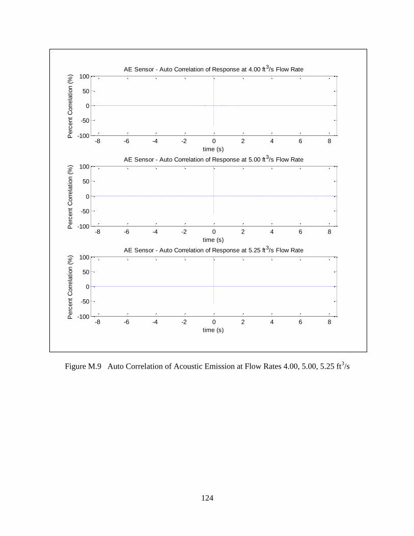
124
Figure M.9 Auto Correlation of Acoustic Emission at Flow Rates 4.00, 5.00, 5.25 ft3/s
-8 -6 -4 -2 0 2 4 6 8-100
-50
0
50
100AE Sensor - Auto Correlation of Response at 4.00 ft3/s Flow Rate
Perc
ent
Corr
ela
tion (
%)
time (s)
-8 -6 -4 -2 0 2 4 6 8-100
-50
0
50
100AE Sensor - Auto Correlation of Response at 5.00 ft3/s Flow Rate
Perc
ent
Corr
ela
tion (
%)
time (s)
-8 -6 -4 -2 0 2 4 6 8-100
-50
0
50
100AE Sensor - Auto Correlation of Response at 5.25 ft3/s Flow Rate
Perc
ent
Corr
ela
tion (
%)
time (s)
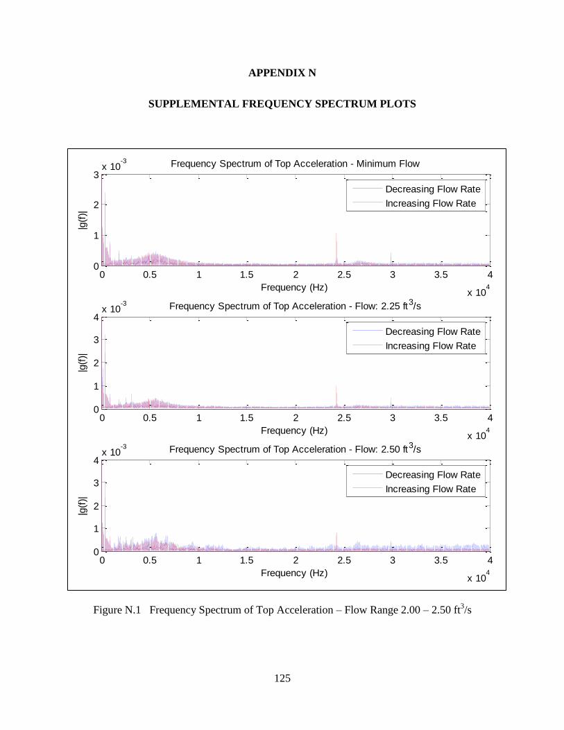
125
APPENDIX N
SUPPLEMENTAL FREQUENCY SPECTRUM PLOTS
Figure N.1 Frequency Spectrum of Top Acceleration – Flow Range 2.00 – 2.50 ft3/s
0 0.5 1 1.5 2 2.5 3 3.5 4
x 104
0
1
2
3x 10
-3
|g(f
)|
Frequency (Hz)
Frequency Spectrum of Top Acceleration - Minimum Flow
Decreasing Flow Rate
Increasing Flow Rate
0 0.5 1 1.5 2 2.5 3 3.5 4
x 104
0
1
2
3
4x 10
-3
|g(f
)|
Frequency (Hz)
Frequency Spectrum of Top Acceleration - Flow: 2.25 ft3/s
Decreasing Flow Rate
Increasing Flow Rate
0 0.5 1 1.5 2 2.5 3 3.5 4
x 104
0
1
2
3
4x 10
-3
|g(f
)|
Frequency (Hz)
Frequency Spectrum of Top Acceleration - Flow: 2.50 ft3/s
Decreasing Flow Rate
Increasing Flow Rate
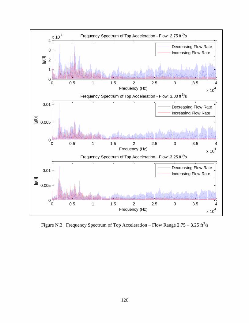
126
Figure N.2 Frequency Spectrum of Top Acceleration – Flow Range 2.75 – 3.25 ft3/s
0 0.5 1 1.5 2 2.5 3 3.5 4
x 104
0
1
2
3
4x 10
-3
|g(f
)|
Frequency (Hz)
Frequency Spectrum of Top Acceleration - Flow: 2.75 ft3/s
Decreasing Flow Rate
Increasing Flow Rate
0 0.5 1 1.5 2 2.5 3 3.5 4
x 104
0
0.005
0.01
|g(f
)|
Frequency (Hz)
Frequency Spectrum of Top Acceleration - Flow: 3.00 ft3/s
Decreasing Flow Rate
Increasing Flow Rate
0 0.5 1 1.5 2 2.5 3 3.5 4
x 104
0
0.005
0.01
|g(f
)|
Frequency (Hz)
Frequency Spectrum of Top Acceleration - Flow: 3.25 ft3/s
Decreasing Flow Rate
Increasing Flow Rate
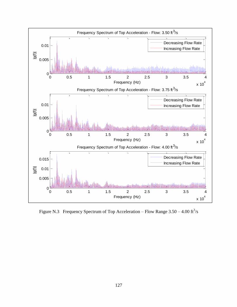
127
Figure N.3 Frequency Spectrum of Top Acceleration – Flow Range 3.50 – 4.00 ft3/s
0 0.5 1 1.5 2 2.5 3 3.5 4
x 104
0
0.005
0.01
|g(f
)|
Frequency (Hz)
Frequency Spectrum of Top Acceleration - Flow: 3.50 ft3/s
Decreasing Flow Rate
Increasing Flow Rate
0 0.5 1 1.5 2 2.5 3 3.5 4
x 104
0
0.005
0.01
|g(f
)|
Frequency (Hz)
Frequency Spectrum of Top Acceleration - Flow: 3.75 ft3/s
Decreasing Flow Rate
Increasing Flow Rate
0 0.5 1 1.5 2 2.5 3 3.5 4
x 104
0
0.005
0.01
0.015
|g(f
)|
Frequency (Hz)
Frequency Spectrum of Top Acceleration - Flow: 4.00 ft3/s
Decreasing Flow Rate
Increasing Flow Rate
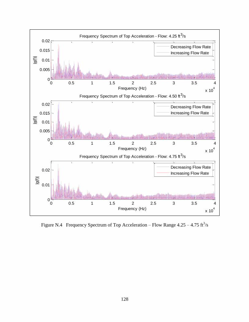
128
Figure N.4 Frequency Spectrum of Top Acceleration – Flow Range 4.25 – 4.75 ft3/s
0 0.5 1 1.5 2 2.5 3 3.5 4
x 104
0
0.005
0.01
0.015
0.02
|g(f
)|
Frequency (Hz)
Frequency Spectrum of Top Acceleration - Flow: 4.25 ft3/s
Decreasing Flow Rate
Increasing Flow Rate
0 0.5 1 1.5 2 2.5 3 3.5 4
x 104
0
0.005
0.01
0.015
0.02
|g(f
)|
Frequency (Hz)
Frequency Spectrum of Top Acceleration - Flow: 4.50 ft3/s
Decreasing Flow Rate
Increasing Flow Rate
0 0.5 1 1.5 2 2.5 3 3.5 4
x 104
0
0.01
0.02
|g(f
)|
Frequency (Hz)
Frequency Spectrum of Top Acceleration - Flow: 4.75 ft3/s
Decreasing Flow Rate
Increasing Flow Rate
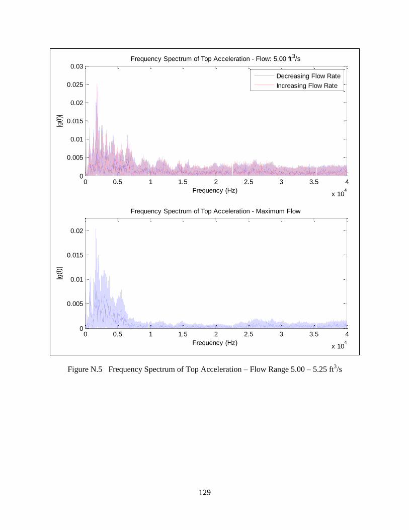
129
Figure N.5 Frequency Spectrum of Top Acceleration – Flow Range 5.00 – 5.25 ft3/s
0 0.5 1 1.5 2 2.5 3 3.5 4
x 104
0
0.005
0.01
0.015
0.02
0.025
0.03|g
(f)|
Frequency (Hz)
Frequency Spectrum of Top Acceleration - Flow: 5.00 ft3/s
Decreasing Flow Rate
Increasing Flow Rate
0 0.5 1 1.5 2 2.5 3 3.5 4
x 104
0
0.005
0.01
0.015
0.02
|g(f
)|
Frequency (Hz)
Frequency Spectrum of Top Acceleration - Maximum Flow
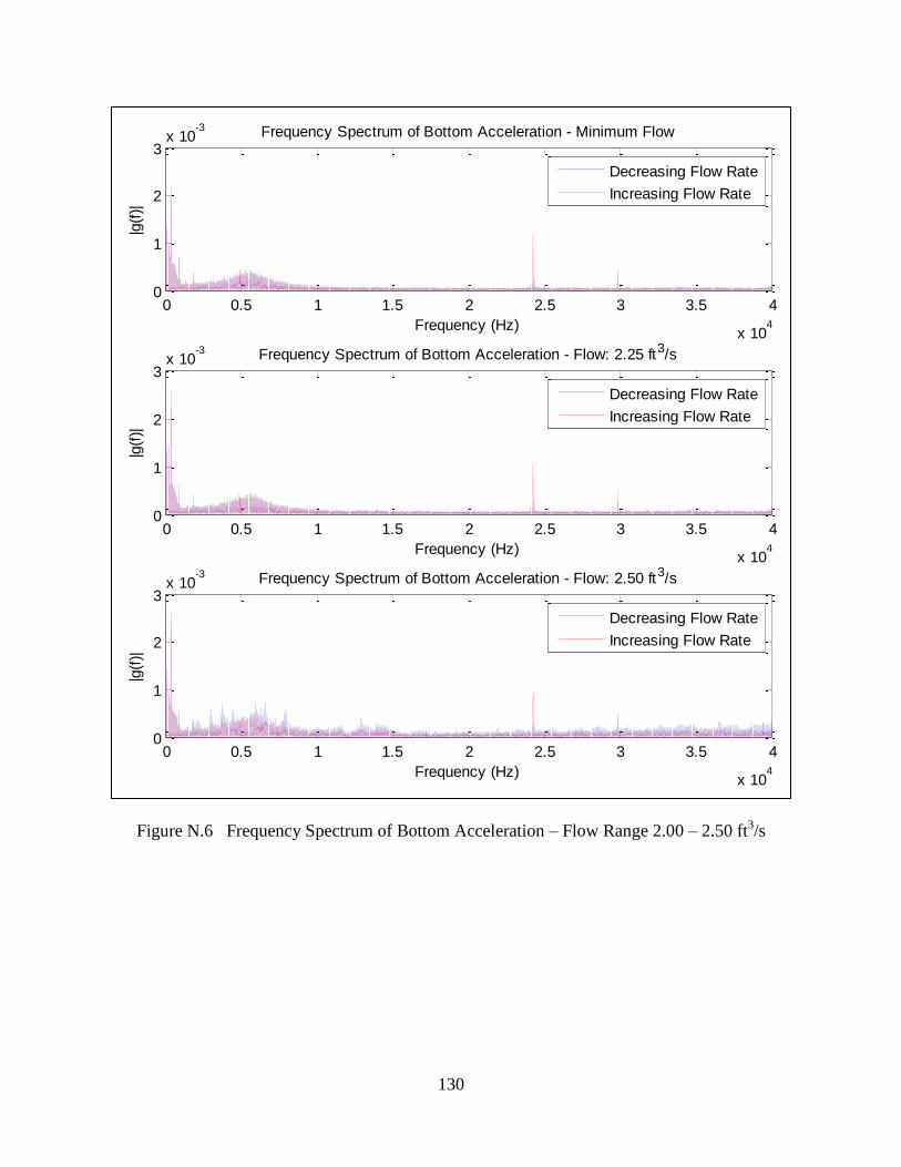
130
Figure N.6 Frequency Spectrum of Bottom Acceleration – Flow Range 2.00 – 2.50 ft3/s
0 0.5 1 1.5 2 2.5 3 3.5 4
x 104
0
1
2
3x 10
-3|g
(f)|
Frequency (Hz)
Frequency Spectrum of Bottom Acceleration - Minimum Flow
Decreasing Flow Rate
Increasing Flow Rate
0 0.5 1 1.5 2 2.5 3 3.5 4
x 104
0
1
2
3x 10
-3
|g(f
)|
Frequency (Hz)
Frequency Spectrum of Bottom Acceleration - Flow: 2.25 ft3/s
Decreasing Flow Rate
Increasing Flow Rate
0 0.5 1 1.5 2 2.5 3 3.5 4
x 104
0
1
2
3x 10
-3
|g(f
)|
Frequency (Hz)
Frequency Spectrum of Bottom Acceleration - Flow: 2.50 ft3/s
Decreasing Flow Rate
Increasing Flow Rate
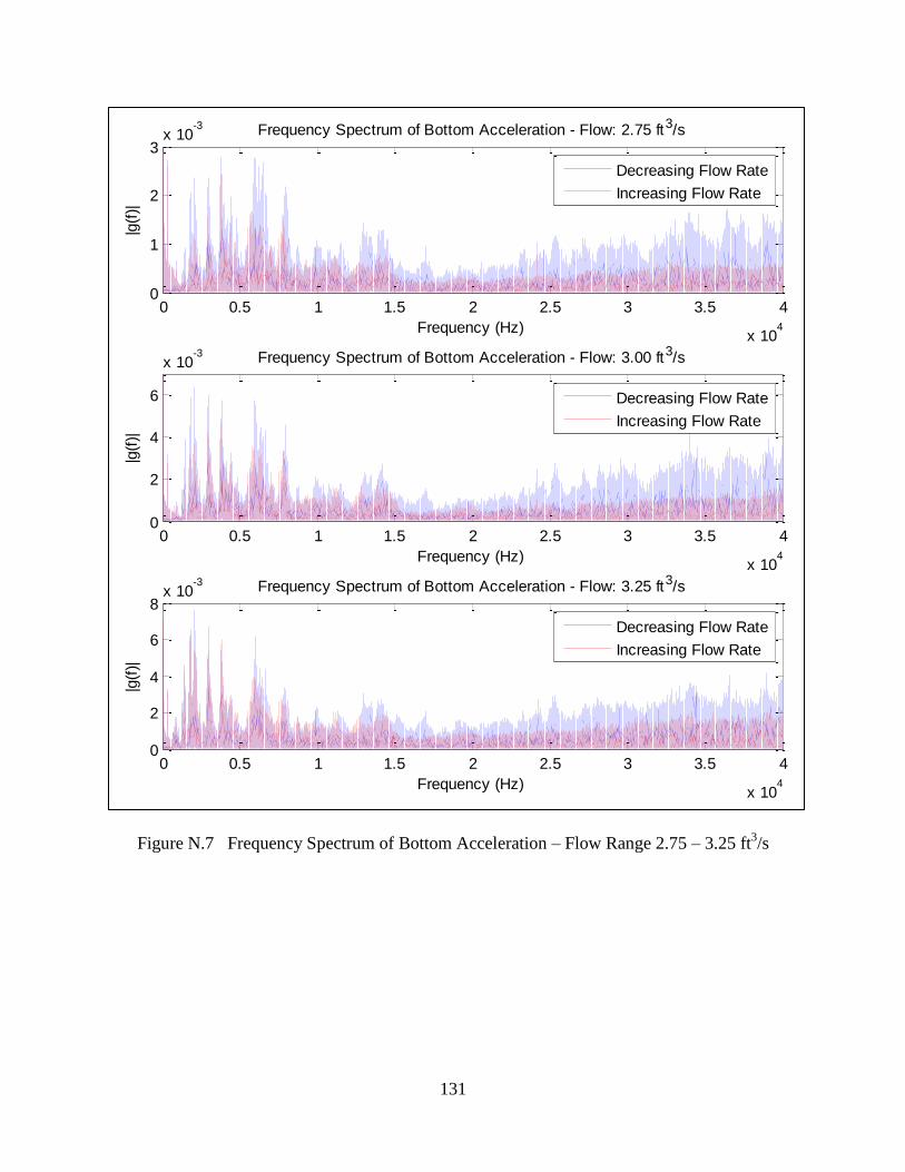
131
Figure N.7 Frequency Spectrum of Bottom Acceleration – Flow Range 2.75 – 3.25 ft3/s
0 0.5 1 1.5 2 2.5 3 3.5 4
x 104
0
1
2
3x 10
-3|g
(f)|
Frequency (Hz)
Frequency Spectrum of Bottom Acceleration - Flow: 2.75 ft3/s
Decreasing Flow Rate
Increasing Flow Rate
0 0.5 1 1.5 2 2.5 3 3.5 4
x 104
0
2
4
6
x 10-3
|g(f
)|
Frequency (Hz)
Frequency Spectrum of Bottom Acceleration - Flow: 3.00 ft3/s
Decreasing Flow Rate
Increasing Flow Rate
0 0.5 1 1.5 2 2.5 3 3.5 4
x 104
0
2
4
6
8x 10
-3
|g(f
)|
Frequency (Hz)
Frequency Spectrum of Bottom Acceleration - Flow: 3.25 ft3/s
Decreasing Flow Rate
Increasing Flow Rate
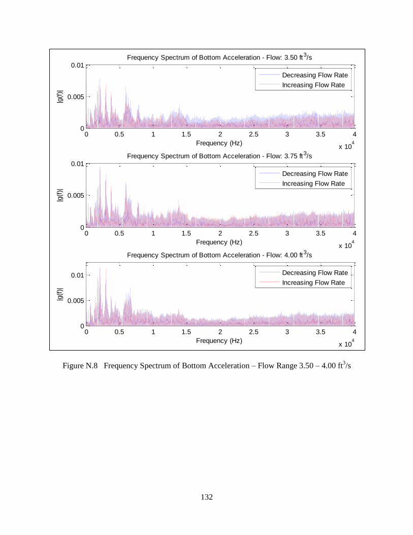
132
Figure N.8 Frequency Spectrum of Bottom Acceleration – Flow Range 3.50 – 4.00 ft3/s
0 0.5 1 1.5 2 2.5 3 3.5 4
x 104
0
0.005
0.01|g
(f)|
Frequency (Hz)
Frequency Spectrum of Bottom Acceleration - Flow: 3.50 ft3/s
Decreasing Flow Rate
Increasing Flow Rate
0 0.5 1 1.5 2 2.5 3 3.5 4
x 104
0
0.005
0.01
|g(f
)|
Frequency (Hz)
Frequency Spectrum of Bottom Acceleration - Flow: 3.75 ft3/s
Decreasing Flow Rate
Increasing Flow Rate
0 0.5 1 1.5 2 2.5 3 3.5 4
x 104
0
0.005
0.01
|g(f
)|
Frequency (Hz)
Frequency Spectrum of Bottom Acceleration - Flow: 4.00 ft3/s
Decreasing Flow Rate
Increasing Flow Rate
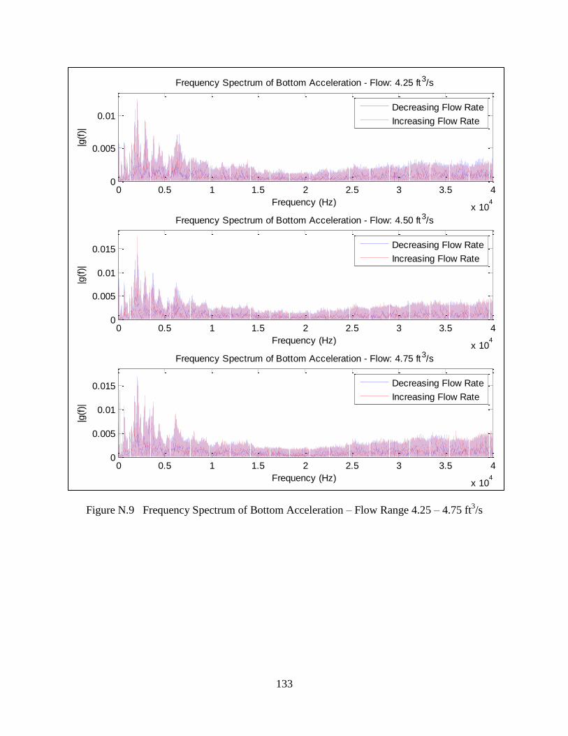
133
Figure N.9 Frequency Spectrum of Bottom Acceleration – Flow Range 4.25 – 4.75 ft3/s
0 0.5 1 1.5 2 2.5 3 3.5 4
x 104
0
0.005
0.01
|g(f
)|
Frequency (Hz)
Frequency Spectrum of Bottom Acceleration - Flow: 4.25 ft3/s
Decreasing Flow Rate
Increasing Flow Rate
0 0.5 1 1.5 2 2.5 3 3.5 4
x 104
0
0.005
0.01
0.015
|g(f
)|
Frequency (Hz)
Frequency Spectrum of Bottom Acceleration - Flow: 4.50 ft3/s
Decreasing Flow Rate
Increasing Flow Rate
0 0.5 1 1.5 2 2.5 3 3.5 4
x 104
0
0.005
0.01
0.015
|g(f
)|
Frequency (Hz)
Frequency Spectrum of Bottom Acceleration - Flow: 4.75 ft3/s
Decreasing Flow Rate
Increasing Flow Rate
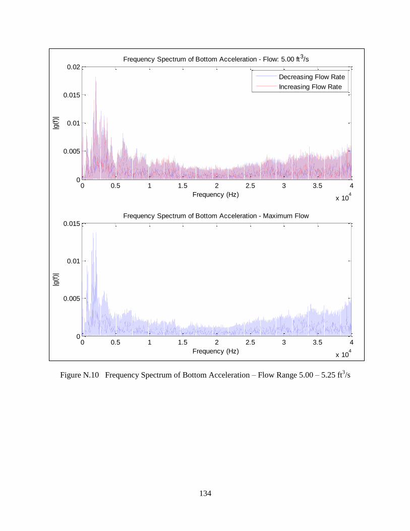
134
Figure N.10 Frequency Spectrum of Bottom Acceleration – Flow Range 5.00 – 5.25 ft3/s
0 0.5 1 1.5 2 2.5 3 3.5 4
x 104
0
0.005
0.01
0.015
0.02
|g(f
)|
Frequency (Hz)
Frequency Spectrum of Bottom Acceleration - Flow: 5.00 ft3/s
Decreasing Flow Rate
Increasing Flow Rate
0 0.5 1 1.5 2 2.5 3 3.5 4
x 104
0
0.005
0.01
0.015
|g(f
)|
Frequency (Hz)
Frequency Spectrum of Bottom Acceleration - Maximum Flow
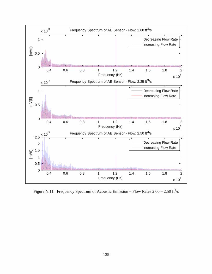
135
Figure N.11 Frequency Spectrum of Acoustic Emission – Flow Rates 2.00 – 2.50 ft3/s
0.4 0.6 0.8 1 1.2 1.4 1.6 1.8 2
x 105
0
0.5
1
x 10-3
Frequency (Hz)
|mV
(f)|
Frequency Spectrum of AE Sensor - Flow: 2.00 ft3/s
0.4 0.6 0.8 1 1.2 1.4 1.6 1.8 2
x 105
0
0.5
1
x 10-3
Frequency (Hz)
|mV
(f)|
Frequency Spectrum of AE Sensor - Flow: 2.25 ft3/s
0.4 0.6 0.8 1 1.2 1.4 1.6 1.8 2
x 105
0
0.5
1
1.5
2
2.5x 10
-3
Frequency (Hz)
|mV
(f)|
Frequency Spectrum of AE Sensor - Flow: 2.50 ft3/s
Decreasing Flow Rate
Increasing Flow Rate
Decreasing Flow Rate
Increasing Flow Rate
Decreasing Flow Rate
Increasing Flow Rate
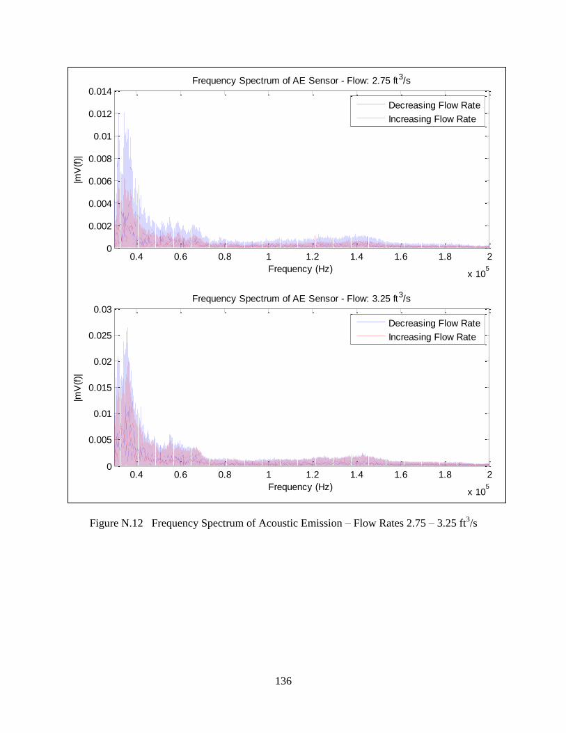
136
Figure N.12 Frequency Spectrum of Acoustic Emission – Flow Rates 2.75 – 3.25 ft3/s
0.4 0.6 0.8 1 1.2 1.4 1.6 1.8 2
x 105
0
0.002
0.004
0.006
0.008
0.01
0.012
0.014
Frequency (Hz)
|mV
(f)|
Frequency Spectrum of AE Sensor - Flow: 2.75 ft3/s
Decreasing Flow Rate
Increasing Flow Rate
0.4 0.6 0.8 1 1.2 1.4 1.6 1.8 2
x 105
0
0.005
0.01
0.015
0.02
0.025
0.03
Frequency (Hz)
|mV
(f)|
Frequency Spectrum of AE Sensor - Flow: 3.25 ft3/s
Decreasing Flow Rate
Increasing Flow Rate
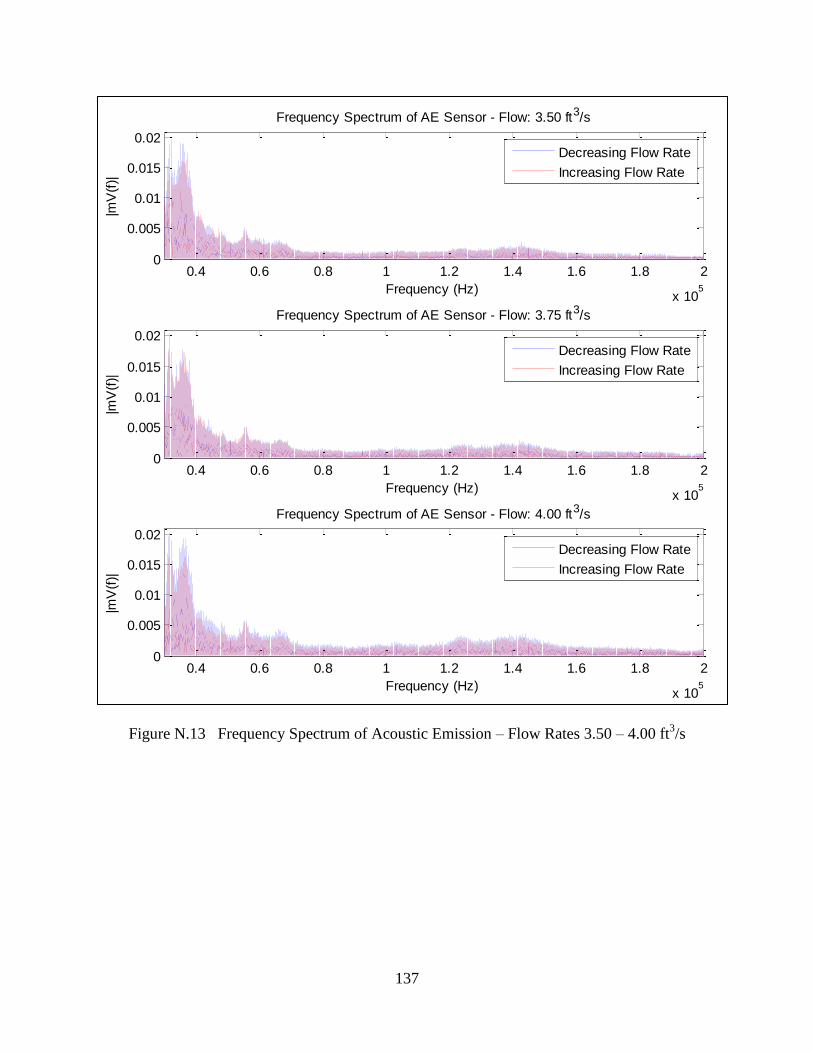
137
Figure N.13 Frequency Spectrum of Acoustic Emission – Flow Rates 3.50 – 4.00 ft3/s
0.4 0.6 0.8 1 1.2 1.4 1.6 1.8 2
x 105
0
0.005
0.01
0.015
0.02
Frequency (Hz)
|mV
(f)|
Frequency Spectrum of AE Sensor - Flow: 3.50 ft3/s
0.4 0.6 0.8 1 1.2 1.4 1.6 1.8 2
x 105
0
0.005
0.01
0.015
0.02
Frequency (Hz)
|mV
(f)|
Frequency Spectrum of AE Sensor - Flow: 3.75 ft3/s
0.4 0.6 0.8 1 1.2 1.4 1.6 1.8 2
x 105
0
0.005
0.01
0.015
0.02
Frequency (Hz)
|mV
(f)|
Frequency Spectrum of AE Sensor - Flow: 4.00 ft3/s
Decreasing Flow Rate
Increasing Flow Rate
Decreasing Flow Rate
Increasing Flow Rate
Decreasing Flow Rate
Increasing Flow Rate
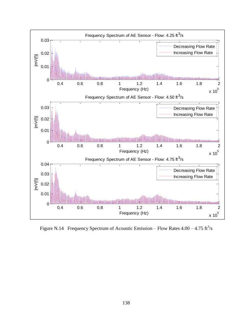
138
Figure N.14 Frequency Spectrum of Acoustic Emission – Flow Rates 4.00 – 4.75 ft3/s
0.4 0.6 0.8 1 1.2 1.4 1.6 1.8 2
x 105
0
0.01
0.02
0.03
Frequency (Hz)
|mV
(f)|
Frequency Spectrum of AE Sensor - Flow: 4.25 ft3/s
0.4 0.6 0.8 1 1.2 1.4 1.6 1.8 2
x 105
0
0.01
0.02
0.03
Frequency (Hz)
|mV
(f)|
Frequency Spectrum of AE Sensor - Flow: 4.50 ft3/s
0.4 0.6 0.8 1 1.2 1.4 1.6 1.8 2
x 105
0
0.01
0.02
0.03
0.04
Frequency (Hz)
|mV
(f)|
Frequency Spectrum of AE Sensor - Flow: 4.75 ft3/s
Decreasing Flow Rate
Increasing Flow Rate
Decreasing Flow Rate
Increasing Flow Rate
Decreasing Flow Rate
Increasing Flow Rate
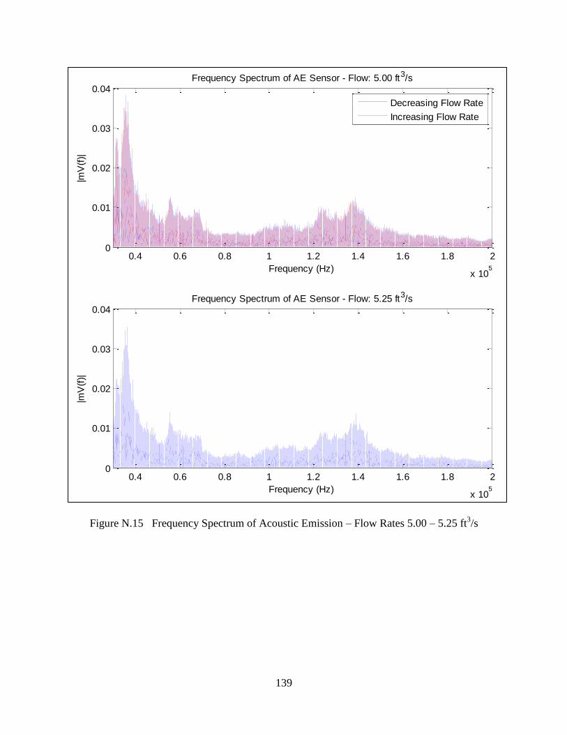
139
Figure N.15 Frequency Spectrum of Acoustic Emission – Flow Rates 5.00 – 5.25 ft3/s
0.4 0.6 0.8 1 1.2 1.4 1.6 1.8 2
x 105
0
0.01
0.02
0.03
0.04
Frequency (Hz)
|mV
(f)|
Frequency Spectrum of AE Sensor - Flow: 5.00 ft3/s
0.4 0.6 0.8 1 1.2 1.4 1.6 1.8 2
x 105
0
0.01
0.02
0.03
0.04
Frequency (Hz)
|mV
(f)|
Frequency Spectrum of AE Sensor - Flow: 5.25 ft3/s
Decreasing Flow Rate
Increasing Flow Rate
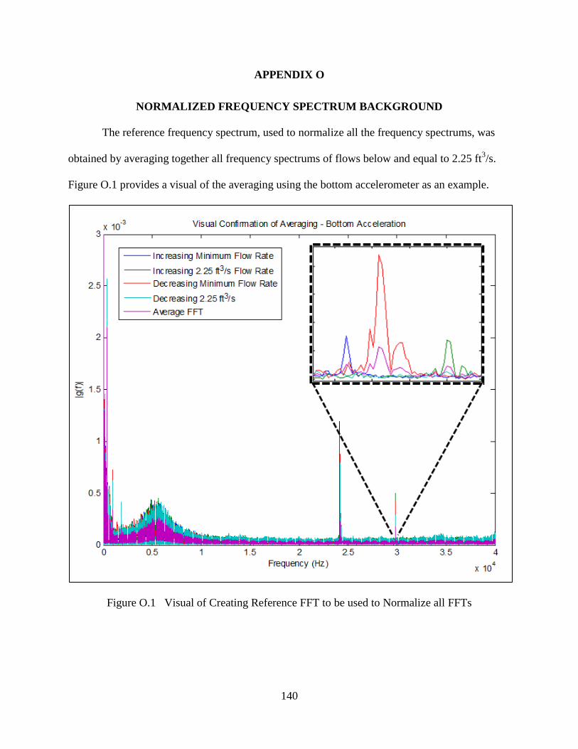
140
APPENDIX O
NORMALIZED FREQUENCY SPECTRUM BACKGROUND
The reference frequency spectrum, used to normalize all the frequency spectrums, was
obtained by averaging together all frequency spectrums of flows below and equal to 2.25 ft3/s.
Figure O.1 provides a visual of the averaging using the bottom accelerometer as an example.
Figure O.1 Visual of Creating Reference FFT to be used to Normalize all FFTs
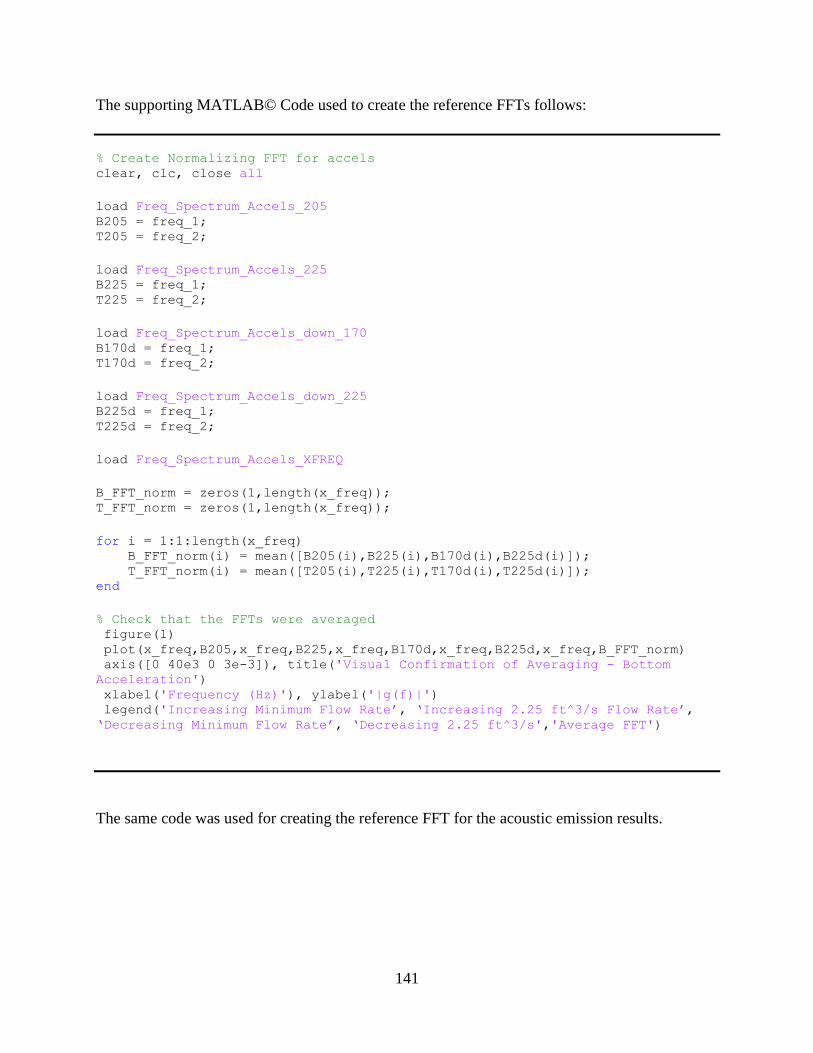
141
The supporting MATLAB© Code used to create the reference FFTs follows:
% Create Normalizing FFT for accels clear, clc, close all
load Freq_Spectrum_Accels_205 B205 = freq_1; T205 = freq_2;
load Freq_Spectrum_Accels_225 B225 = freq_1; T225 = freq_2;
load Freq_Spectrum_Accels_down_170 B170d = freq_1; T170d = freq_2;
load Freq_Spectrum_Accels_down_225 B225d = freq_1; T225d = freq_2;
load Freq_Spectrum_Accels_XFREQ
B_FFT_norm = zeros(1,length(x_freq)); T_FFT_norm = zeros(1,length(x_freq));
for i = 1:1:length(x_freq) B_FFT_norm(i) = mean([B205(i),B225(i),B170d(i),B225d(i)]); T_FFT_norm(i) = mean([T205(i),T225(i),T170d(i),T225d(i)]); end
% Check that the FFTs were averaged figure(1) plot(x_freq,B205,x_freq,B225,x_freq,B170d,x_freq,B225d,x_freq,B_FFT_norm) axis([0 40e3 0 3e-3]), title('Visual Confirmation of Averaging - Bottom
Acceleration') xlabel('Frequency (Hz)'), ylabel('|g(f)|') legend('Increasing Minimum Flow Rate’, ‘Increasing 2.25 ft^3/s Flow Rate’,
‘Decreasing Minimum Flow Rate’, ‘Decreasing 2.25 ft^3/s','Average FFT')
The same code was used for creating the reference FFT for the acoustic emission results.
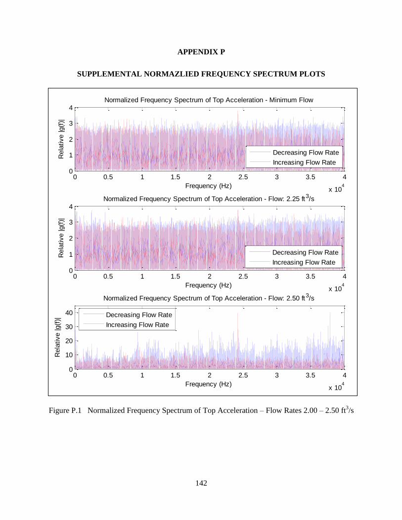
142
APPENDIX P
SUPPLEMENTAL NORMAZLIED FREQUENCY SPECTRUM PLOTS
Figure P.1 Normalized Frequency Spectrum of Top Acceleration – Flow Rates 2.00 – 2.50 ft3/s
0 0.5 1 1.5 2 2.5 3 3.5 4
x 104
0
1
2
3
4
Rela
tive |g(f
)|
Frequency (Hz)
Normalized Frequency Spectrum of Top Acceleration - Minimum Flow
0 0.5 1 1.5 2 2.5 3 3.5 4
x 104
0
1
2
3
4
Rela
tive |g(f
)|
Frequency (Hz)
Normalized Frequency Spectrum of Top Acceleration - Flow: 2.25 ft3/s
0 0.5 1 1.5 2 2.5 3 3.5 4
x 104
0
10
20
30
40
Rela
tive |g(f
)|
Frequency (Hz)
Normalized Frequency Spectrum of Top Acceleration - Flow: 2.50 ft3/s
Decreasing Flow Rate
Increasing Flow Rate
Decreasing Flow Rate
Increasing Flow Rate
Decreasing Flow Rate
Increasing Flow Rate
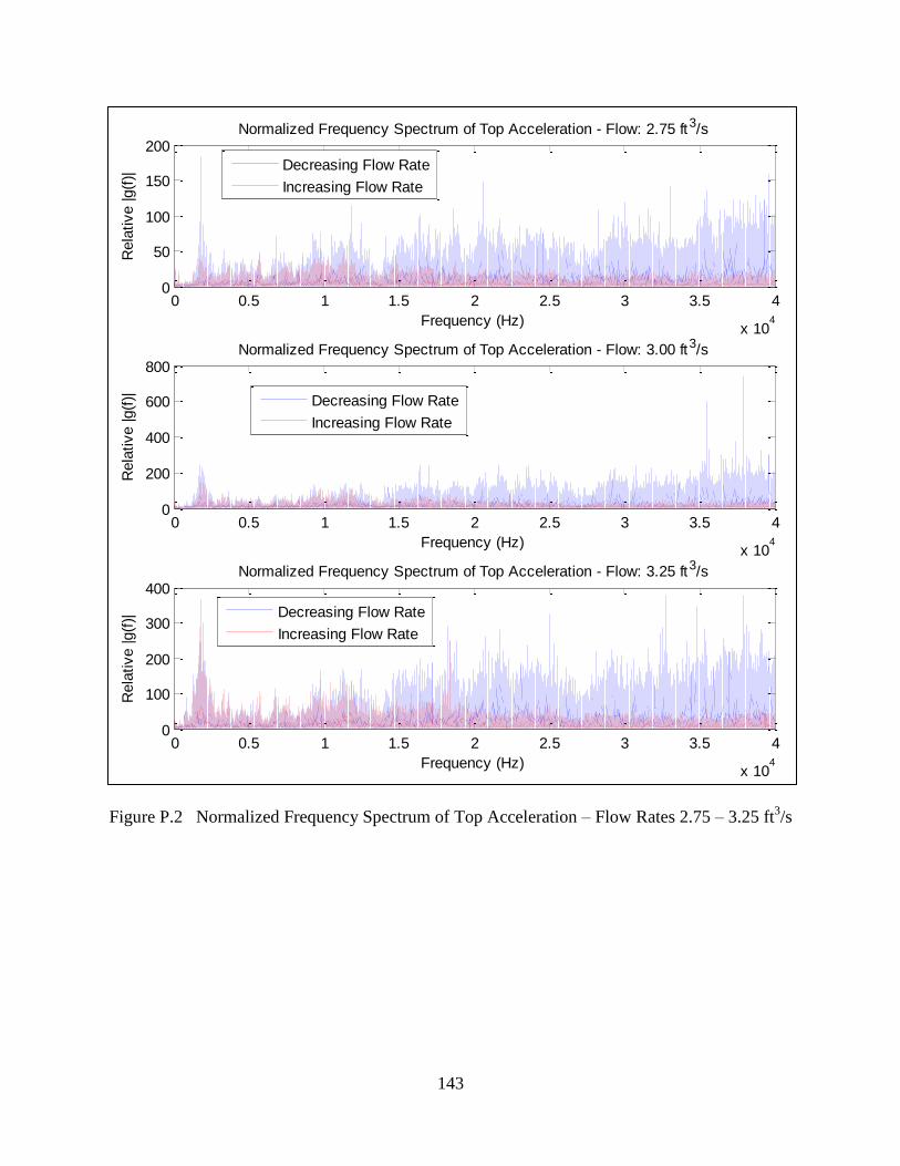
143
Figure P.2 Normalized Frequency Spectrum of Top Acceleration – Flow Rates 2.75 – 3.25 ft3/s
0 0.5 1 1.5 2 2.5 3 3.5 4
x 104
0
50
100
150
200
Rela
tive |g(f
)|
Frequency (Hz)
Normalized Frequency Spectrum of Top Acceleration - Flow: 2.75 ft3/s
0 0.5 1 1.5 2 2.5 3 3.5 4
x 104
0
200
400
600
800
Rela
tive |g(f
)|
Frequency (Hz)
Normalized Frequency Spectrum of Top Acceleration - Flow: 3.00 ft3/s
0 0.5 1 1.5 2 2.5 3 3.5 4
x 104
0
100
200
300
400
Rela
tive |g(f
)|
Frequency (Hz)
Normalized Frequency Spectrum of Top Acceleration - Flow: 3.25 ft3/s
Decreasing Flow Rate
Increasing Flow Rate
Decreasing Flow Rate
Increasing Flow Rate
Decreasing Flow Rate
Increasing Flow Rate
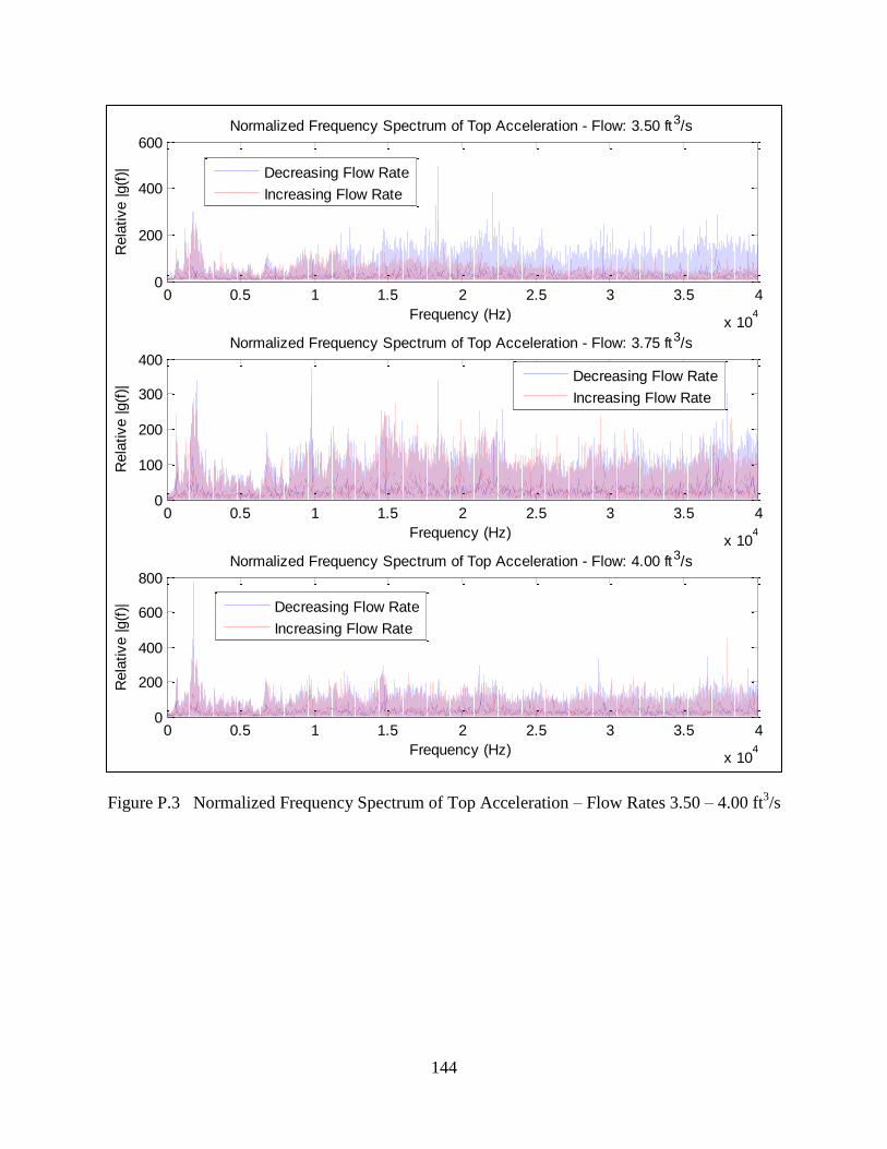
144
Figure P.3 Normalized Frequency Spectrum of Top Acceleration – Flow Rates 3.50 – 4.00 ft3/s
0 0.5 1 1.5 2 2.5 3 3.5 4
x 104
0
200
400
600
Rela
tive |g(f
)|
Frequency (Hz)
Normalized Frequency Spectrum of Top Acceleration - Flow: 3.50 ft3/s
Decreasing Flow Rate
Increasing Flow Rate
0 0.5 1 1.5 2 2.5 3 3.5 4
x 104
0
100
200
300
400
Rela
tive |g(f
)|
Frequency (Hz)
Normalized Frequency Spectrum of Top Acceleration - Flow: 3.75 ft3/s
Decreasing Flow Rate
Increasing Flow Rate
0 0.5 1 1.5 2 2.5 3 3.5 4
x 104
0
200
400
600
800
Rela
tive |g(f
)|
Frequency (Hz)
Normalized Frequency Spectrum of Top Acceleration - Flow: 4.00 ft3/s
Decreasing Flow Rate
Increasing Flow Rate
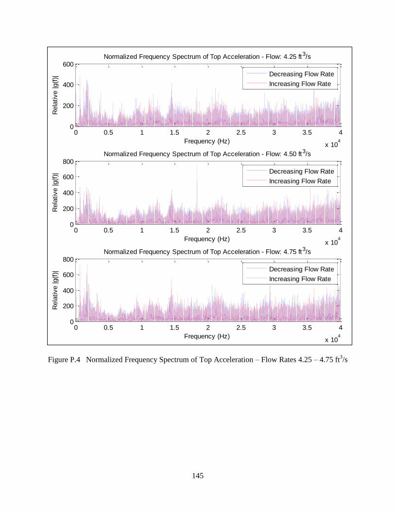
145
Figure P.4 Normalized Frequency Spectrum of Top Acceleration – Flow Rates 4.25 – 4.75 ft3/s
0 0.5 1 1.5 2 2.5 3 3.5 4
x 104
0
200
400
600
Rela
tive |g(f
)|
Frequency (Hz)
Normalized Frequency Spectrum of Top Acceleration - Flow: 4.25 ft3/s
Decreasing Flow Rate
Increasing Flow Rate
0 0.5 1 1.5 2 2.5 3 3.5 4
x 104
0
200
400
600
800
Rela
tive |g(f
)|
Frequency (Hz)
Normalized Frequency Spectrum of Top Acceleration - Flow: 4.50 ft3/s
Decreasing Flow Rate
Increasing Flow Rate
0 0.5 1 1.5 2 2.5 3 3.5 4
x 104
0
200
400
600
800
Rela
tive |g(f
)|
Frequency (Hz)
Normalized Frequency Spectrum of Top Acceleration - Flow: 4.75 ft3/s
Decreasing Flow Rate
Increasing Flow Rate
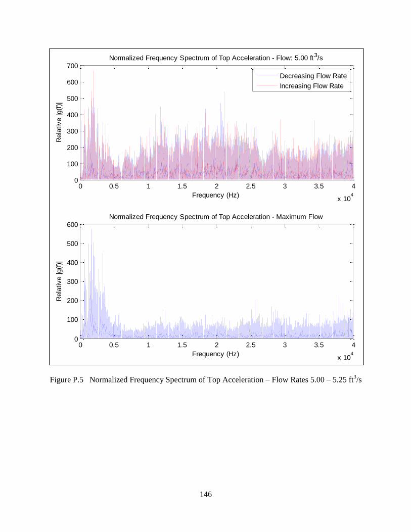
146
Figure P.5 Normalized Frequency Spectrum of Top Acceleration – Flow Rates 5.00 – 5.25 ft3/s
0 0.5 1 1.5 2 2.5 3 3.5 4
x 104
0
100
200
300
400
500
600
700R
ela
tive |g(f
)|
Frequency (Hz)
Normalized Frequency Spectrum of Top Acceleration - Flow: 5.00 ft3/s
Decreasing Flow Rate
Increasing Flow Rate
0 0.5 1 1.5 2 2.5 3 3.5 4
x 104
0
100
200
300
400
500
600
Rela
tive |g(f
)|
Frequency (Hz)
Normalized Frequency Spectrum of Top Acceleration - Maximum Flow
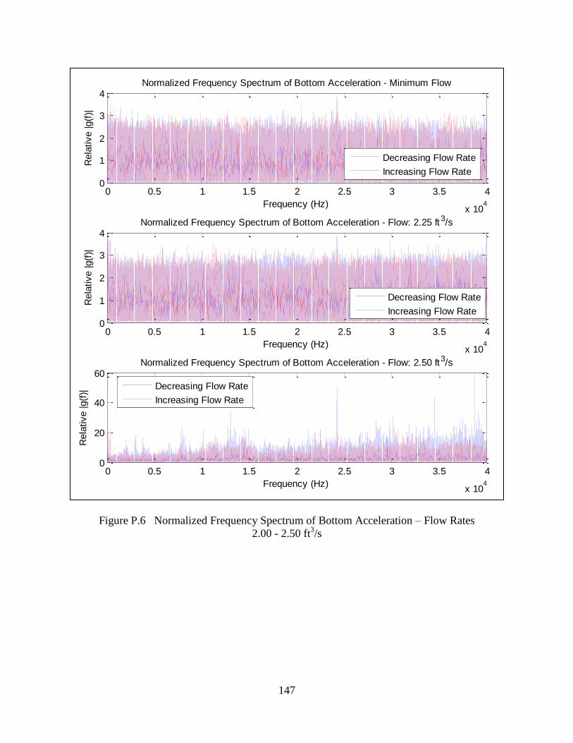
147
Figure P.6 Normalized Frequency Spectrum of Bottom Acceleration – Flow Rates
2.00 - 2.50 ft3/s
0 0.5 1 1.5 2 2.5 3 3.5 4
x 104
0
1
2
3
4R
ela
tive |g(f
)|
Frequency (Hz)
Normalized Frequency Spectrum of Bottom Acceleration - Minimum Flow
Decreasing Flow Rate
Increasing Flow Rate
0 0.5 1 1.5 2 2.5 3 3.5 4
x 104
0
1
2
3
4
Rela
tive |g(f
)|
Frequency (Hz)
Normalized Frequency Spectrum of Bottom Acceleration - Flow: 2.25 ft3/s
Decreasing Flow Rate
Increasing Flow Rate
0 0.5 1 1.5 2 2.5 3 3.5 4
x 104
0
20
40
60
Rela
tive |g(f
)|
Frequency (Hz)
Normalized Frequency Spectrum of Bottom Acceleration - Flow: 2.50 ft3/s
Decreasing Flow Rate
Increasing Flow Rate
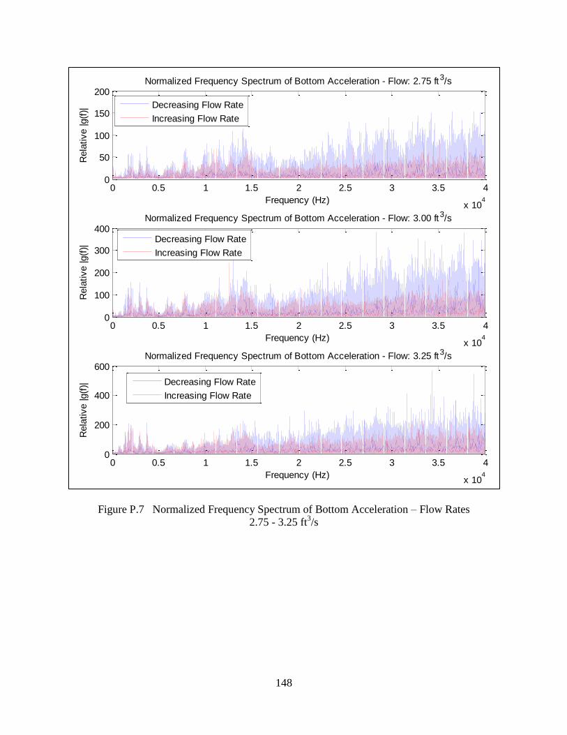
148
Figure P.7 Normalized Frequency Spectrum of Bottom Acceleration – Flow Rates
2.75 - 3.25 ft3/s
0 0.5 1 1.5 2 2.5 3 3.5 4
x 104
0
50
100
150
200R
ela
tive |g(f
)|
Frequency (Hz)
Normalized Frequency Spectrum of Bottom Acceleration - Flow: 2.75 ft3/s
Decreasing Flow Rate
Increasing Flow Rate
0 0.5 1 1.5 2 2.5 3 3.5 4
x 104
0
100
200
300
400
Rela
tive |g(f
)|
Frequency (Hz)
Normalized Frequency Spectrum of Bottom Acceleration - Flow: 3.00 ft3/s
Decreasing Flow Rate
Increasing Flow Rate
0 0.5 1 1.5 2 2.5 3 3.5 4
x 104
0
200
400
600
Rela
tive |g(f
)|
Frequency (Hz)
Normalized Frequency Spectrum of Bottom Acceleration - Flow: 3.25 ft3/s
Decreasing Flow Rate
Increasing Flow Rate
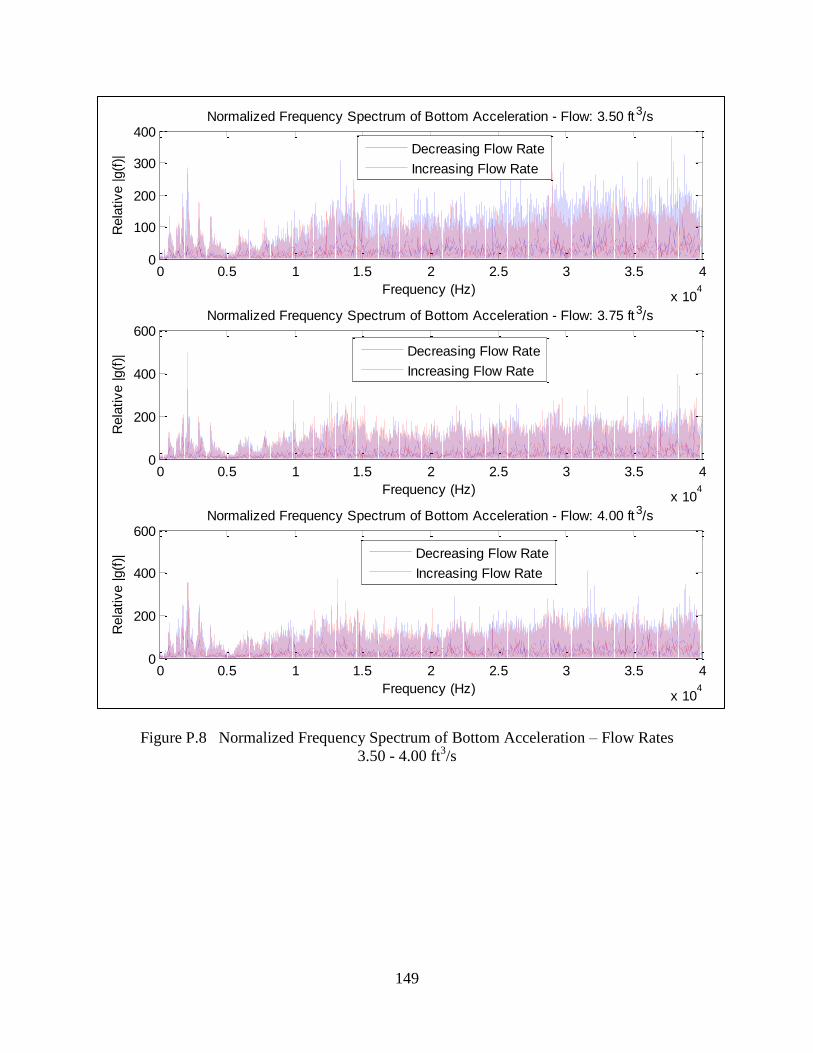
149
Figure P.8 Normalized Frequency Spectrum of Bottom Acceleration – Flow Rates
3.50 - 4.00 ft3/s
0 0.5 1 1.5 2 2.5 3 3.5 4
x 104
0
100
200
300
400R
ela
tive |g(f
)|
Frequency (Hz)
Normalized Frequency Spectrum of Bottom Acceleration - Flow: 3.50 ft3/s
Decreasing Flow Rate
Increasing Flow Rate
0 0.5 1 1.5 2 2.5 3 3.5 4
x 104
0
200
400
600
Rela
tive |g(f
)|
Frequency (Hz)
Normalized Frequency Spectrum of Bottom Acceleration - Flow: 3.75 ft3/s
Decreasing Flow Rate
Increasing Flow Rate
0 0.5 1 1.5 2 2.5 3 3.5 4
x 104
0
200
400
600
Rela
tive |g(f
)|
Frequency (Hz)
Normalized Frequency Spectrum of Bottom Acceleration - Flow: 4.00 ft3/s
Decreasing Flow Rate
Increasing Flow Rate
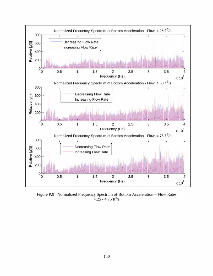
150
Figure P.9 Normalized Frequency Spectrum of Bottom Acceleration – Flow Rates
4.25 - 4.75 ft3/s
0 0.5 1 1.5 2 2.5 3 3.5 4
x 104
0
200
400
600
800
Rela
tive |g(f
)|
Frequency (Hz)
Normalized Frequency Spectrum of Bottom Acceleration - Flow: 4.25 ft3/s
Decreasing Flow Rate
Increasing Flow Rate
0 0.5 1 1.5 2 2.5 3 3.5 4
x 104
0
200
400
600
800
Rela
tive |g(f
)|
Frequency (Hz)
Normalized Frequency Spectrum of Bottom Acceleration - Flow: 4.50 ft3/s
Decreasing Flow Rate
Increasing Flow Rate
0 0.5 1 1.5 2 2.5 3 3.5 4
x 104
0
200
400
600
800
Rela
tive |g(f
)|
Frequency (Hz)
Normalized Frequency Spectrum of Bottom Acceleration - Flow: 4.75 ft3/s
Decreasing Flow Rate
Increasing Flow Rate
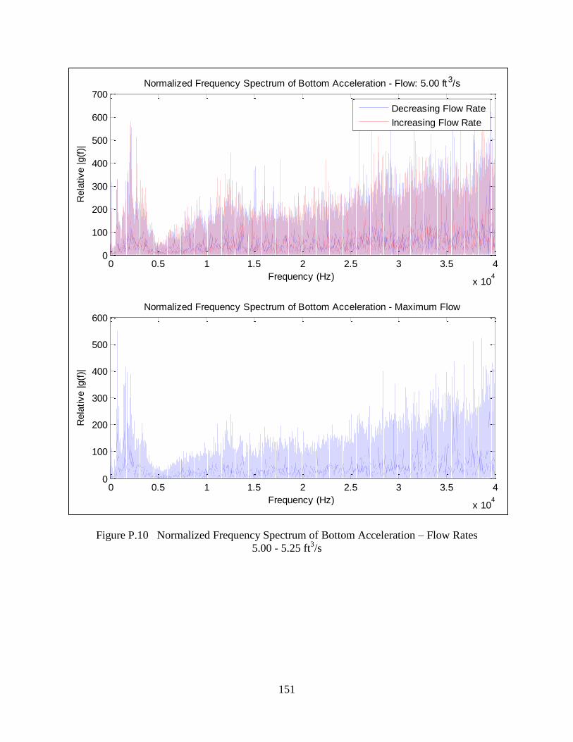
151
Figure P.10 Normalized Frequency Spectrum of Bottom Acceleration – Flow Rates
5.00 - 5.25 ft3/s
0 0.5 1 1.5 2 2.5 3 3.5 4
x 104
0
100
200
300
400
500
600
700
Rela
tive |g(f
)|
Frequency (Hz)
Normalized Frequency Spectrum of Bottom Acceleration - Flow: 5.00 ft3/s
Decreasing Flow Rate
Increasing Flow Rate
0 0.5 1 1.5 2 2.5 3 3.5 4
x 104
0
100
200
300
400
500
600
Rela
tive |g(f
)|
Frequency (Hz)
Normalized Frequency Spectrum of Bottom Acceleration - Maximum Flow
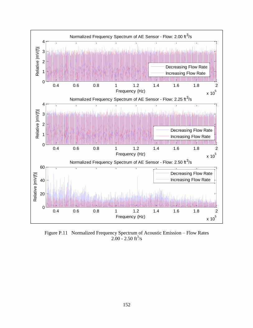
152
Figure P.11 Normalized Frequency Spectrum of Acoustic Emission – Flow Rates
2.00 - 2.50 ft3/s
0.4 0.6 0.8 1 1.2 1.4 1.6 1.8 2
x 105
0
1
2
3
4
Frequency (Hz)
Rela
tive |m
V(f
)|Normalized Frequency Spectrum of AE Sensor - Flow: 2.00 ft3/s
0.4 0.6 0.8 1 1.2 1.4 1.6 1.8 2
x 105
0
1
2
3
4
Frequency (Hz)
Rela
tive |m
V(f
)|
Normalized Frequency Spectrum of AE Sensor - Flow: 2.25 ft3/s
0.4 0.6 0.8 1 1.2 1.4 1.6 1.8 2
x 105
0
20
40
60
Frequency (Hz)
Rela
tive |m
V(f
)|
Normalized Frequency Spectrum of AE Sensor - Flow: 2.50 ft3/s
Decreasing Flow Rate
Increasing Flow Rate
Decreasing Flow Rate
Increasing Flow Rate
Decreasing Flow Rate
Increasing Flow Rate
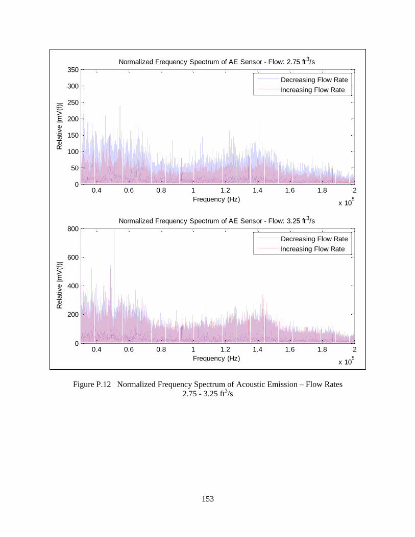
153
Figure P.12 Normalized Frequency Spectrum of Acoustic Emission – Flow Rates
2.75 - 3.25 ft3/s
0.4 0.6 0.8 1 1.2 1.4 1.6 1.8 2
x 105
0
50
100
150
200
250
300
350
Frequency (Hz)
Rela
tive |m
V(f
)|Normalized Frequency Spectrum of AE Sensor - Flow: 2.75 ft3/s
0.4 0.6 0.8 1 1.2 1.4 1.6 1.8 2
x 105
0
200
400
600
800
Frequency (Hz)
Rela
tive |m
V(f
)|
Normalized Frequency Spectrum of AE Sensor - Flow: 3.25 ft3/s
Decreasing Flow Rate
Increasing Flow Rate
Decreasing Flow Rate
Increasing Flow Rate
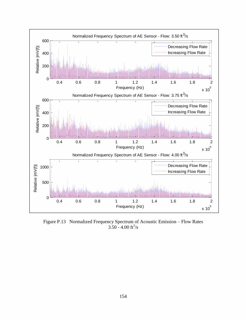
154
Figure P.13 Normalized Frequency Spectrum of Acoustic Emission – Flow Rates
3.50 - 4.00 ft3/s
0.4 0.6 0.8 1 1.2 1.4 1.6 1.8 2
x 105
0
200
400
600
Frequency (Hz)
Rela
tive |m
V(f
)|Normalized Frequency Spectrum of AE Sensor - Flow: 3.50 ft3/s
0.4 0.6 0.8 1 1.2 1.4 1.6 1.8 2
x 105
0
200
400
600
Frequency (Hz)
Rela
tive |m
V(f
)|
Normalized Frequency Spectrum of AE Sensor - Flow: 3.75 ft3/s
0.4 0.6 0.8 1 1.2 1.4 1.6 1.8 2
x 105
0
500
1000
Frequency (Hz)
Rela
tive |m
V(f
)|
Normalized Frequency Spectrum of AE Sensor - Flow: 4.00 ft3/s
Decreasing Flow Rate
Increasing Flow Rate
Decreasing Flow Rate
Increasing Flow Rate
Decreasing Flow Rate
Increasing Flow Rate
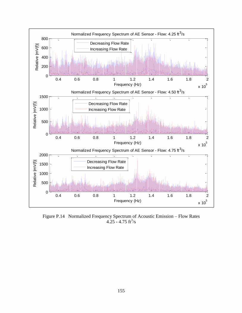
155
Figure P.14 Normalized Frequency Spectrum of Acoustic Emission – Flow Rates
4.25 - 4.75 ft3/s
0.4 0.6 0.8 1 1.2 1.4 1.6 1.8 2
x 105
0
200
400
600
800
Frequency (Hz)
Rela
tive |m
V(f
)|Normalized Frequency Spectrum of AE Sensor - Flow: 4.25 ft3/s
Decreasing Flow Rate
Increasing Flow Rate
0.4 0.6 0.8 1 1.2 1.4 1.6 1.8 2
x 105
0
500
1000
1500
Frequency (Hz)
Rela
tive |m
V(f
)|
Normalized Frequency Spectrum of AE Sensor - Flow: 4.50 ft3/s
Decreasing Flow Rate
Increasing Flow Rate
0.4 0.6 0.8 1 1.2 1.4 1.6 1.8 2
x 105
0
500
1000
1500
2000
Frequency (Hz)
Rela
tive |m
V(f
)|
Normalized Frequency Spectrum of AE Sensor - Flow: 4.75 ft3/s
Decreasing Flow Rate
Increasing Flow Rate
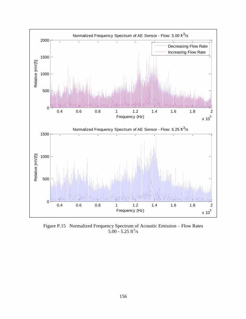
156
Figure P.15 Normalized Frequency Spectrum of Acoustic Emission – Flow Rates
5.00 - 5.25 ft3/s
0.4 0.6 0.8 1 1.2 1.4 1.6 1.8 2
x 105
0
500
1000
1500
2000
Frequency (Hz)
Rela
tive |m
V(f
)|Normalized Frequency Spectrum of AE Sensor - Flow: 5.00 ft3/s
Decreasing Flow Rate
Increasing Flow Rate
0.4 0.6 0.8 1 1.2 1.4 1.6 1.8 2
x 105
0
500
1000
1500
Frequency (Hz)
Rela
tive |m
V(f
)|
Normalized Frequency Spectrum of AE Sensor - Flow: 5.25 ft3/s
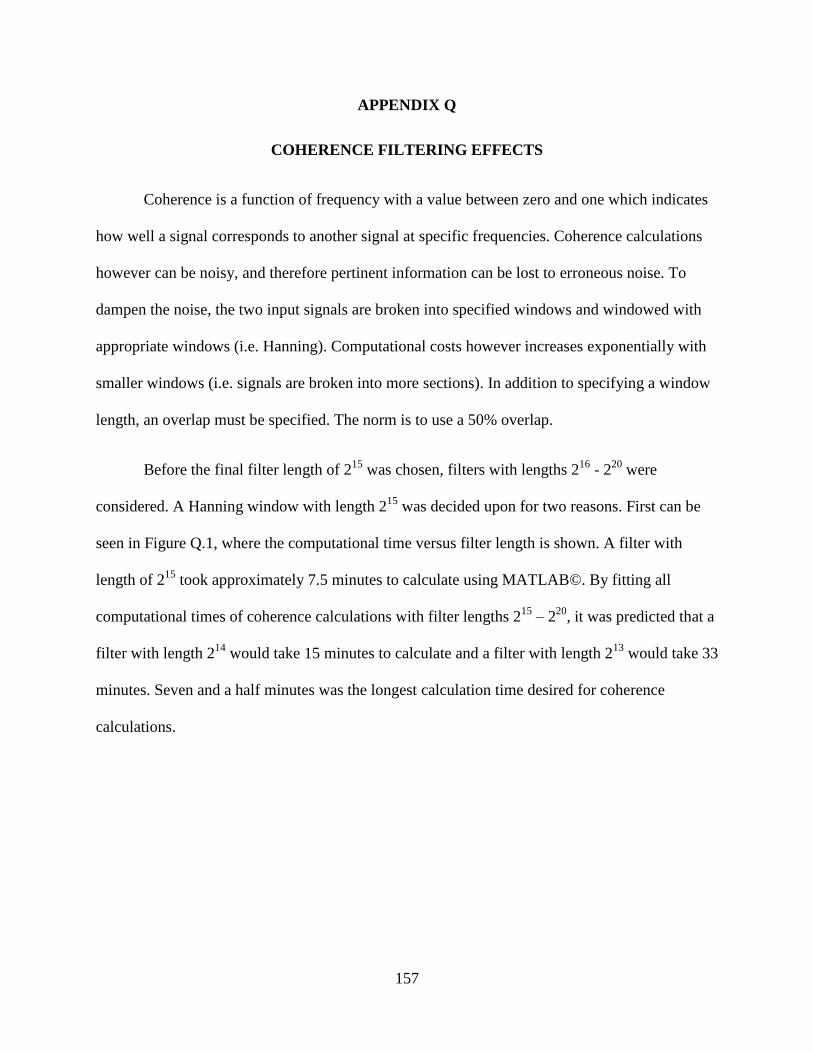
157
APPENDIX Q
COHERENCE FILTERING EFFECTS
Coherence is a function of frequency with a value between zero and one which indicates
how well a signal corresponds to another signal at specific frequencies. Coherence calculations
however can be noisy, and therefore pertinent information can be lost to erroneous noise. To
dampen the noise, the two input signals are broken into specified windows and windowed with
appropriate windows (i.e. Hanning). Computational costs however increases exponentially with
smaller windows (i.e. signals are broken into more sections). In addition to specifying a window
length, an overlap must be specified. The norm is to use a 50% overlap.
Before the final filter length of 215
was chosen, filters with lengths 216
- 220
were
considered. A Hanning window with length 215
was decided upon for two reasons. First can be
seen in Figure Q.1, where the computational time versus filter length is shown. A filter with
length of 215
took approximately 7.5 minutes to calculate using MATLAB©. By fitting all
computational times of coherence calculations with filter lengths 215
– 220
, it was predicted that a
filter with length 214
would take 15 minutes to calculate and a filter with length 213
would take 33
minutes. Seven and a half minutes was the longest calculation time desired for coherence
calculations.
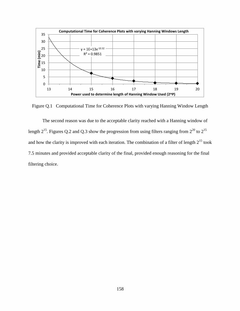
158
Figure Q.1 Computational Time for Coherence Plots with varying Hanning Window Length
The second reason was due to the acceptable clarity reached with a Hanning window of
length 215
. Figures Q.2 and Q.3 show the progression from using filters ranging from 220
to 215
and how the clarity is improved with each iteration. The combination of a filter of length 215
took
7.5 minutes and provided acceptable clarity of the final, provided enough reasoning for the final
filtering choice.
y = 1E+13x-10.32 R² = 0.9851
0
5
10
15
20
25
30
35
13 14 15 16 17 18 19 20
Tim
e (
min
)
Power used to determine length of Hanning Window Used (2^P)
Computational Time for Coherence Plots with varying Hanning Windows Length
159
Figure Q.2 Coherence between Top and Bottom Acceleration with Hanning Window of varying Length 220
– 218
0 0.5 1 1.5 2 2.5 3 3.5 4
x 104
0
0.5
1Coherence between Top and Bottom Accelerometers - Flow Rate 5.00 ft3/s - Signal Windowed with Hanning Window - Length 220
Frequency (Hz)
Magnitude
0 0.5 1 1.5 2 2.5 3 3.5 4
x 104
0
0.5
1Coherence between Top and Bottom Accelerometers - Flow Rate 5.00 ft3/s - Signal Windowed with Hanning Window - Length 219
Frequency (Hz)
Magnitude
0 0.5 1 1.5 2 2.5 3 3.5 4
x 104
0
0.5
1Coherence between Top and Bottom Accelerometers - Flow Rate 5.00 ft3/s - Signal Windowed with Hanning Window - Length 218
Frequency (Hz)
Magnitude
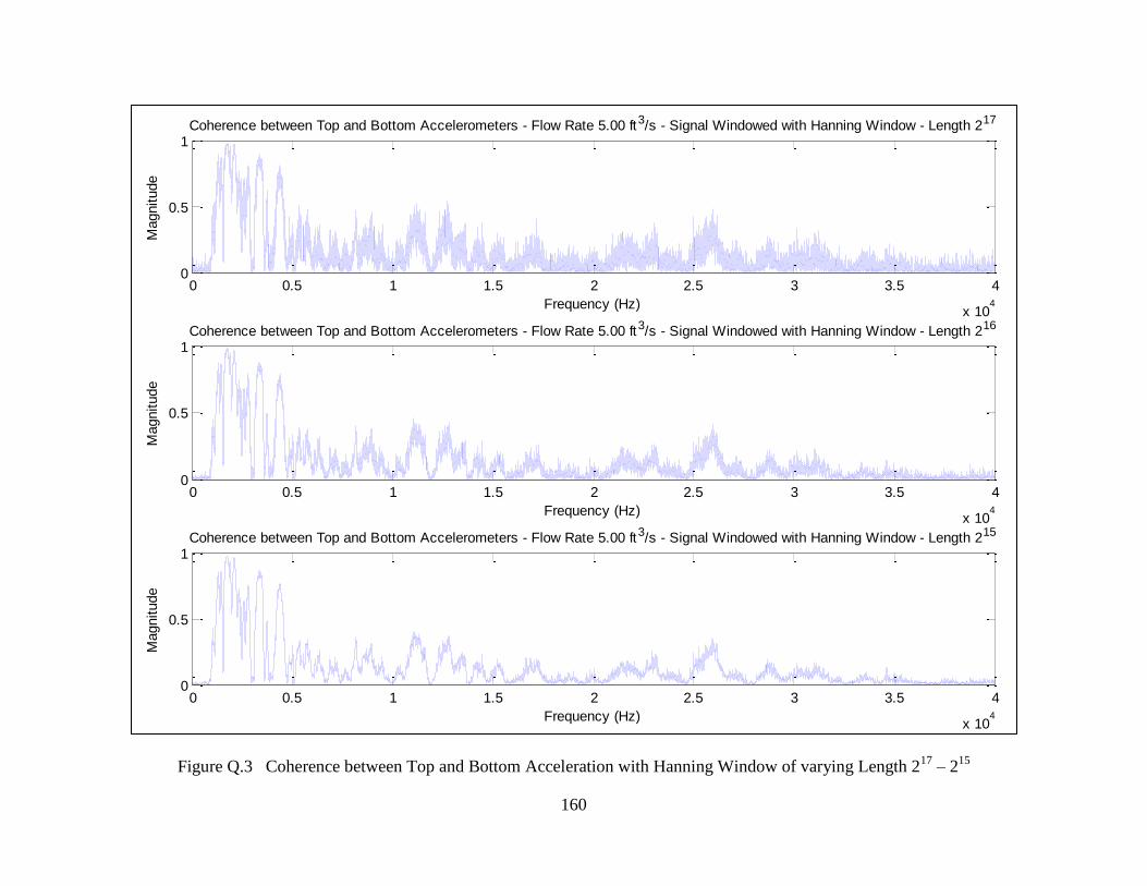
160
Figure Q.3 Coherence between Top and Bottom Acceleration with Hanning Window of varying Length 217
– 215
0 0.5 1 1.5 2 2.5 3 3.5 4
x 104
0
0.5
1Coherence between Top and Bottom Accelerometers - Flow Rate 5.00 ft3/s - Signal Windowed with Hanning Window - Length 217
Frequency (Hz)
Magnitude
0 0.5 1 1.5 2 2.5 3 3.5 4
x 104
0
0.5
1Coherence between Top and Bottom Accelerometers - Flow Rate 5.00 ft3/s - Signal Windowed with Hanning Window - Length 216
Frequency (Hz)
Magnitude
0 0.5 1 1.5 2 2.5 3 3.5 4
x 104
0
0.5
1Coherence between Top and Bottom Accelerometers - Flow Rate 5.00 ft3/s - Signal Windowed with Hanning Window - Length 215
Frequency (Hz)
Magnitude
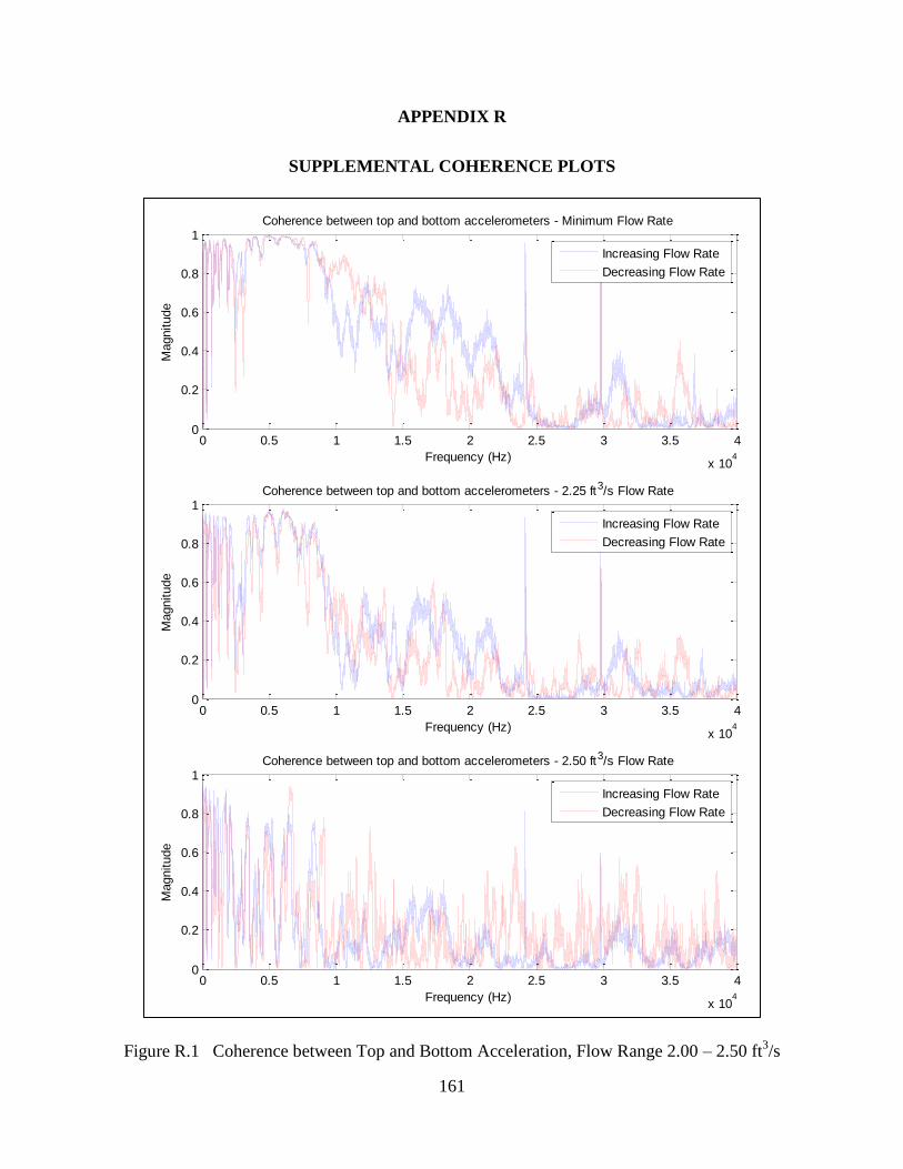
161
APPENDIX R
SUPPLEMENTAL COHERENCE PLOTS
Figure R.1 Coherence between Top and Bottom Acceleration, Flow Range 2.00 – 2.50 ft3/s
0 0.5 1 1.5 2 2.5 3 3.5 4
x 104
0
0.2
0.4
0.6
0.8
1
Frequency (Hz)
Magnitude
Coherence between top and bottom accelerometers - Minimum Flow Rate
Increasing Flow Rate
Decreasing Flow Rate
0 0.5 1 1.5 2 2.5 3 3.5 4
x 104
0
0.2
0.4
0.6
0.8
1
Frequency (Hz)
Magnitude
Coherence between top and bottom accelerometers - 2.25 ft3/s Flow Rate
Increasing Flow Rate
Decreasing Flow Rate
0 0.5 1 1.5 2 2.5 3 3.5 4
x 104
0
0.2
0.4
0.6
0.8
1
Frequency (Hz)
Magnitude
Coherence between top and bottom accelerometers - 2.50 ft3/s Flow Rate
Increasing Flow Rate
Decreasing Flow Rate
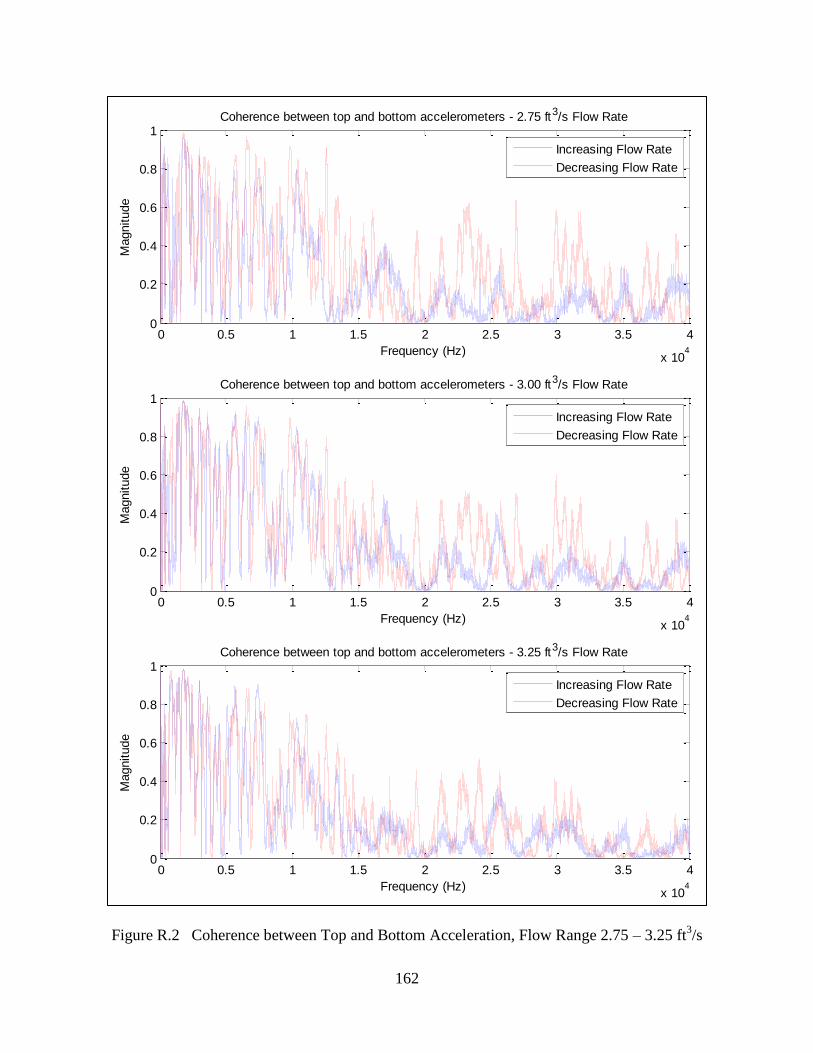
162
Figure R.2 Coherence between Top and Bottom Acceleration, Flow Range 2.75 – 3.25 ft3/s
0 0.5 1 1.5 2 2.5 3 3.5 4
x 104
0
0.2
0.4
0.6
0.8
1
Frequency (Hz)
Magnitude
Coherence between top and bottom accelerometers - 2.75 ft3/s Flow Rate
Increasing Flow Rate
Decreasing Flow Rate
0 0.5 1 1.5 2 2.5 3 3.5 4
x 104
0
0.2
0.4
0.6
0.8
1
Frequency (Hz)
Magnitude
Coherence between top and bottom accelerometers - 3.00 ft3/s Flow Rate
Increasing Flow Rate
Decreasing Flow Rate
0 0.5 1 1.5 2 2.5 3 3.5 4
x 104
0
0.2
0.4
0.6
0.8
1
Frequency (Hz)
Magnitude
Coherence between top and bottom accelerometers - 3.25 ft3/s Flow Rate
Increasing Flow Rate
Decreasing Flow Rate
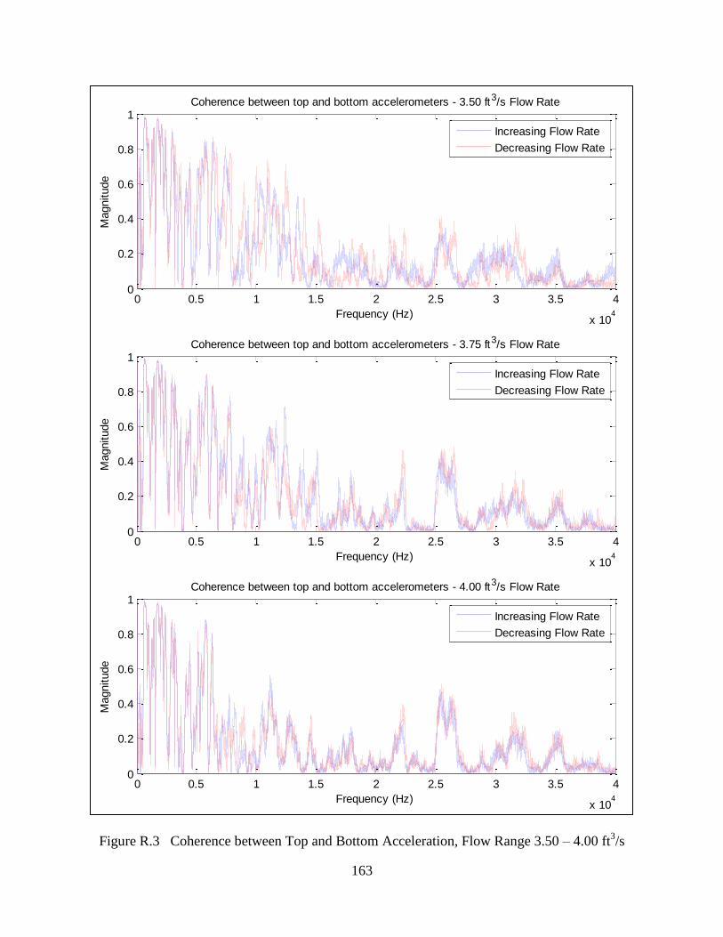
163
Figure R.3 Coherence between Top and Bottom Acceleration, Flow Range 3.50 – 4.00 ft3/s
0 0.5 1 1.5 2 2.5 3 3.5 4
x 104
0
0.2
0.4
0.6
0.8
1
Frequency (Hz)
Magnitude
Coherence between top and bottom accelerometers - 3.50 ft3/s Flow Rate
Increasing Flow Rate
Decreasing Flow Rate
0 0.5 1 1.5 2 2.5 3 3.5 4
x 104
0
0.2
0.4
0.6
0.8
1
Frequency (Hz)
Magnitude
Coherence between top and bottom accelerometers - 3.75 ft3/s Flow Rate
Increasing Flow Rate
Decreasing Flow Rate
0 0.5 1 1.5 2 2.5 3 3.5 4
x 104
0
0.2
0.4
0.6
0.8
1
Frequency (Hz)
Magnitude
Coherence between top and bottom accelerometers - 4.00 ft3/s Flow Rate
Increasing Flow Rate
Decreasing Flow Rate
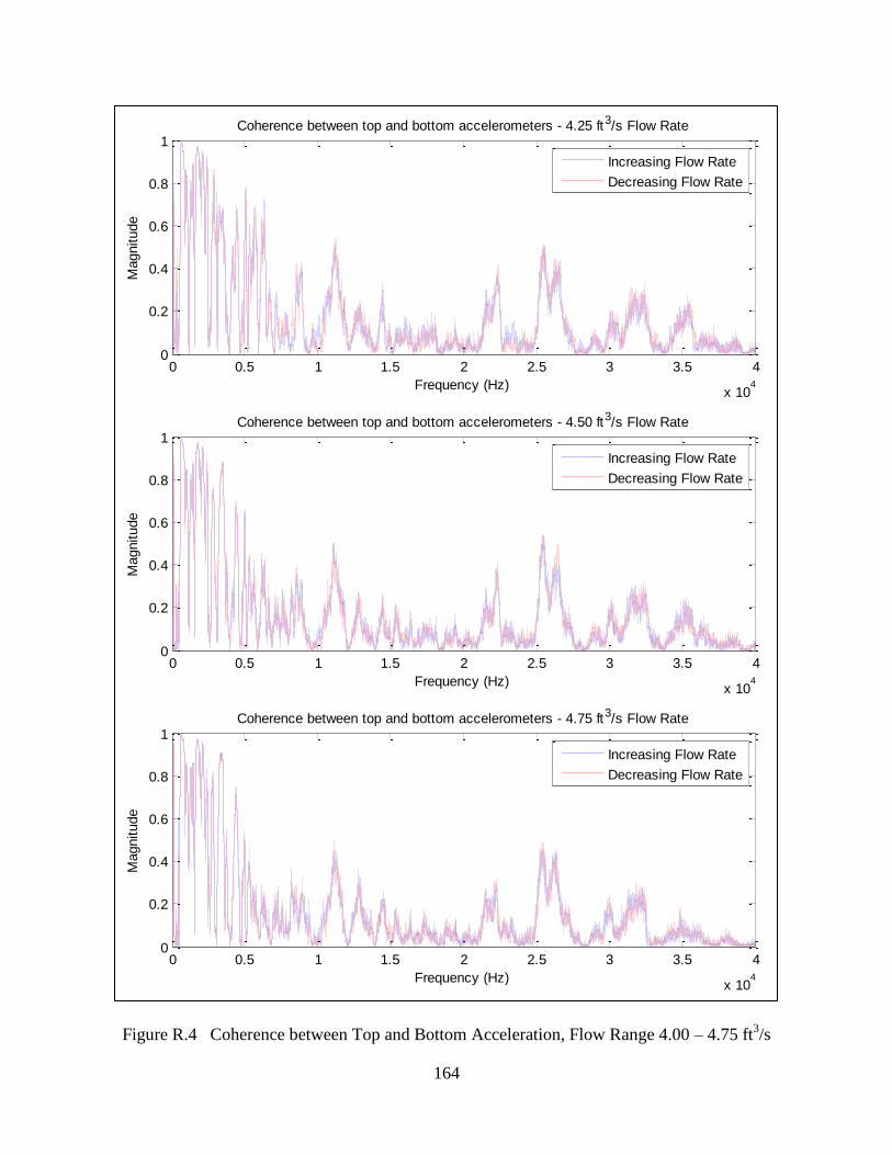
164
Figure R.4 Coherence between Top and Bottom Acceleration, Flow Range 4.00 – 4.75 ft3/s
0 0.5 1 1.5 2 2.5 3 3.5 4
x 104
0
0.2
0.4
0.6
0.8
1
Frequency (Hz)
Magnitude
Coherence between top and bottom accelerometers - 4.25 ft3/s Flow Rate
Increasing Flow Rate
Decreasing Flow Rate
0 0.5 1 1.5 2 2.5 3 3.5 4
x 104
0
0.2
0.4
0.6
0.8
1
Frequency (Hz)
Magnitude
Coherence between top and bottom accelerometers - 4.50 ft3/s Flow Rate
Increasing Flow Rate
Decreasing Flow Rate
0 0.5 1 1.5 2 2.5 3 3.5 4
x 104
0
0.2
0.4
0.6
0.8
1
Frequency (Hz)
Magnitude
Coherence between top and bottom accelerometers - 4.75 ft3/s Flow Rate
Increasing Flow Rate
Decreasing Flow Rate
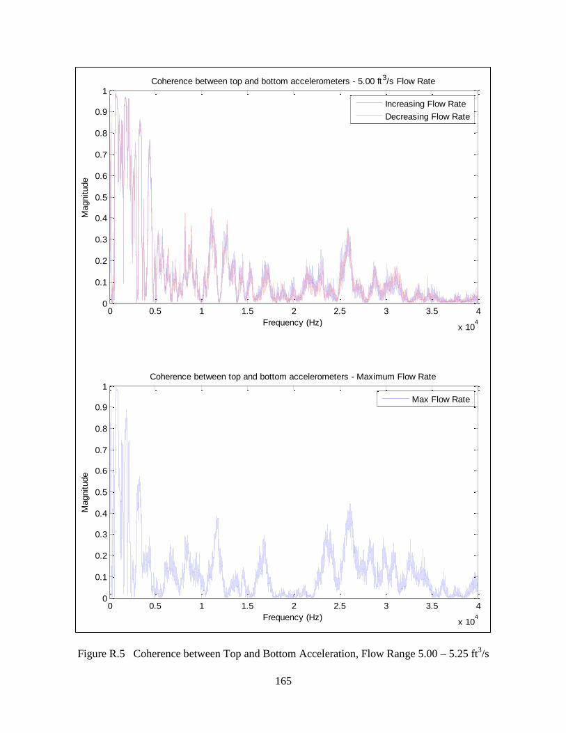
165
Figure R.5 Coherence between Top and Bottom Acceleration, Flow Range 5.00 – 5.25 ft3/s
0 0.5 1 1.5 2 2.5 3 3.5 4
x 104
0
0.1
0.2
0.3
0.4
0.5
0.6
0.7
0.8
0.9
1
Frequency (Hz)
Magnitude
Coherence between top and bottom accelerometers - 5.00 ft3/s Flow Rate
Increasing Flow Rate
Decreasing Flow Rate
0 0.5 1 1.5 2 2.5 3 3.5 4
x 104
0
0.1
0.2
0.3
0.4
0.5
0.6
0.7
0.8
0.9
1
Frequency (Hz)
Magnitude
Coherence between top and bottom accelerometers - Maximum Flow Rate
Max Flow Rate
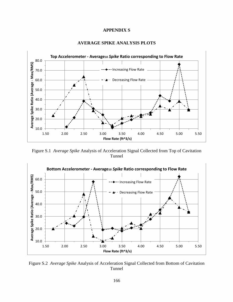
166
APPENDIX S
AVERAGE SPIKE ANALYSIS PLOTS
Figure S.1 Average Spike Analysis of Acceleration Signal Collected from Top of Cavitation
Tunnel
Figure S.2 Average Spike Analysis of Acceleration Signal Collected from Bottom of Cavitation
Tunnel
10.0
20.0
30.0
40.0
50.0
60.0
70.0
80.0
1.50 2.00 2.50 3.00 3.50 4.00 4.50 5.00 5.50
Ave
rage
Sp
ike
Rat
io (
Ave
rage
- M
ax/R
MS)
Flow Rate (ft^3/s)
Top Accelerometer - Average10 Spike Ratio corresponding to Flow Rate
Increasing Flow Rate
Decreasing Flow Rate
10.0
20.0
30.0
40.0
50.0
60.0
1.50 2.00 2.50 3.00 3.50 4.00 4.50 5.00 5.50
Ave
rage
Sp
ike
Rat
io (
Ave
rage
- M
ax/R
MS)
Flow Rate (ft^3/s)
Bottom Accelerometer - Average10 Spike Ratio corresponding to Flow Rate
Increasing Flow Rate
Decreasing Flow Rate
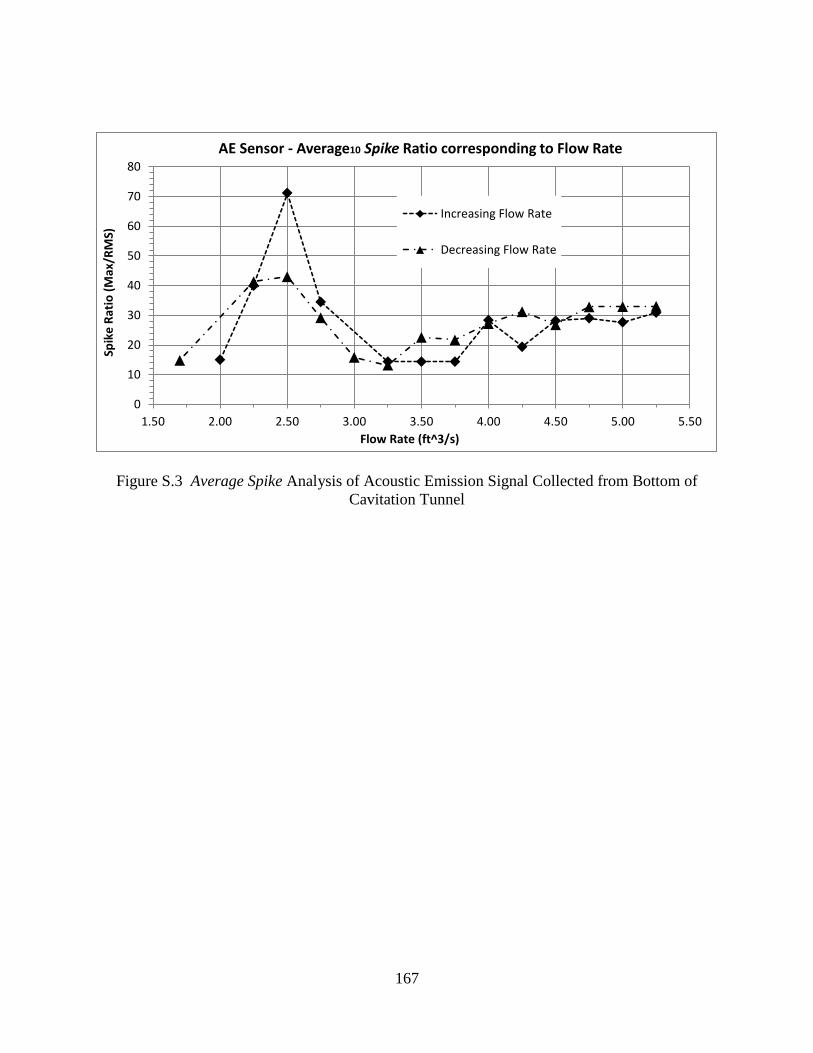
167
Figure S.3 Average Spike Analysis of Acoustic Emission Signal Collected from Bottom of
Cavitation Tunnel
0
10
20
30
40
50
60
70
80
1.50 2.00 2.50 3.00 3.50 4.00 4.50 5.00 5.50
Spik
e R
atio
(M
ax/R
MS)
Flow Rate (ft^3/s)
AE Sensor - Average10 Spike Ratio corresponding to Flow Rate
Increasing Flow Rate
Decreasing Flow Rate
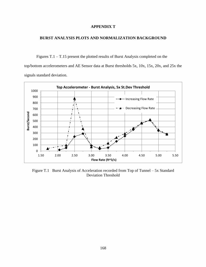
168
APPENDIX T
BURST ANALYSIS PLOTS AND NORMALIZATION BACKGROUND
Figures T.1 – T.15 present the plotted results of Burst Analysis completed on the
top/bottom accelerometers and AE Sensor data at Burst thresholds 5x, 10x, 15x, 20x, and 25x the
signals standard deviation.
Figure T.1 Burst Analysis of Acceleration recorded from Top of Tunnel – 5x Standard
Deviation Threshold
0
100
200
300
400
500
600
700
800
900
1000
1.50 2.00 2.50 3.00 3.50 4.00 4.50 5.00 5.50
Bu
rst/
Seco
nd
Flow Rate (ft^3/s)
Top Accelerometer - Burst Analysis, 5x St.Dev Threshold
Increasing Flow Rate
Decreasing Flow Rate
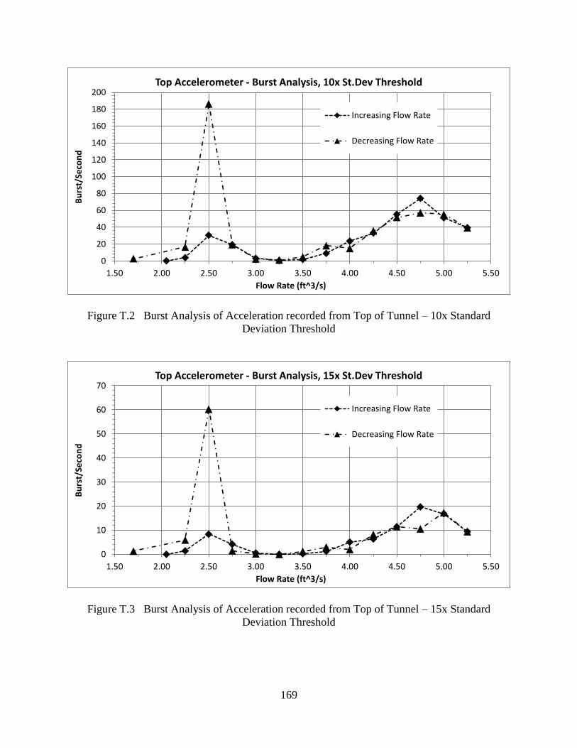
169
Figure T.2 Burst Analysis of Acceleration recorded from Top of Tunnel – 10x Standard
Deviation Threshold
Figure T.3 Burst Analysis of Acceleration recorded from Top of Tunnel – 15x Standard
Deviation Threshold
0
20
40
60
80
100
120
140
160
180
200
1.50 2.00 2.50 3.00 3.50 4.00 4.50 5.00 5.50
Bu
rst/
Seco
nd
Flow Rate (ft^3/s)
Top Accelerometer - Burst Analysis, 10x St.Dev Threshold
Increasing Flow Rate
Decreasing Flow Rate
0
10
20
30
40
50
60
70
1.50 2.00 2.50 3.00 3.50 4.00 4.50 5.00 5.50
Bu
rst/
Seco
nd
Flow Rate (ft^3/s)
Top Accelerometer - Burst Analysis, 15x St.Dev Threshold
Increasing Flow Rate
Decreasing Flow Rate
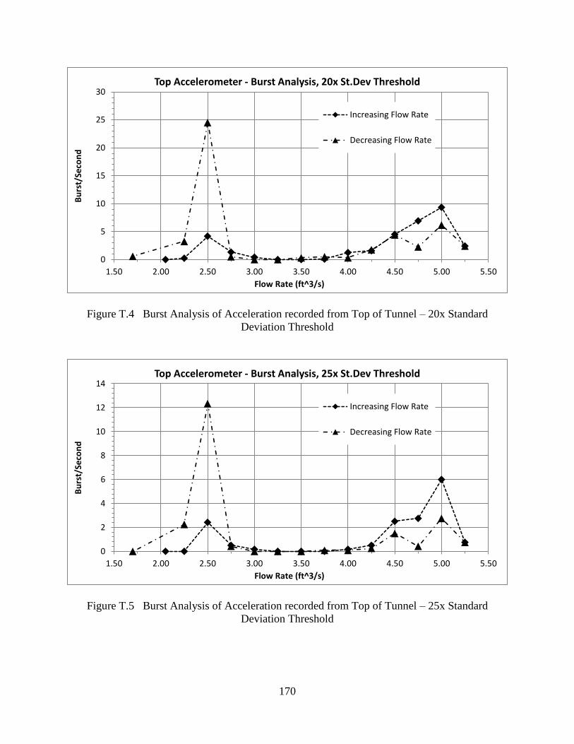
170
Figure T.4 Burst Analysis of Acceleration recorded from Top of Tunnel – 20x Standard
Deviation Threshold
Figure T.5 Burst Analysis of Acceleration recorded from Top of Tunnel – 25x Standard
Deviation Threshold
0
5
10
15
20
25
30
1.50 2.00 2.50 3.00 3.50 4.00 4.50 5.00 5.50
Bu
rst/
Seco
nd
Flow Rate (ft^3/s)
Top Accelerometer - Burst Analysis, 20x St.Dev Threshold
Increasing Flow Rate
Decreasing Flow Rate
0
2
4
6
8
10
12
14
1.50 2.00 2.50 3.00 3.50 4.00 4.50 5.00 5.50
Bu
rst/
Seco
nd
Flow Rate (ft^3/s)
Top Accelerometer - Burst Analysis, 25x St.Dev Threshold
Increasing Flow Rate
Decreasing Flow Rate
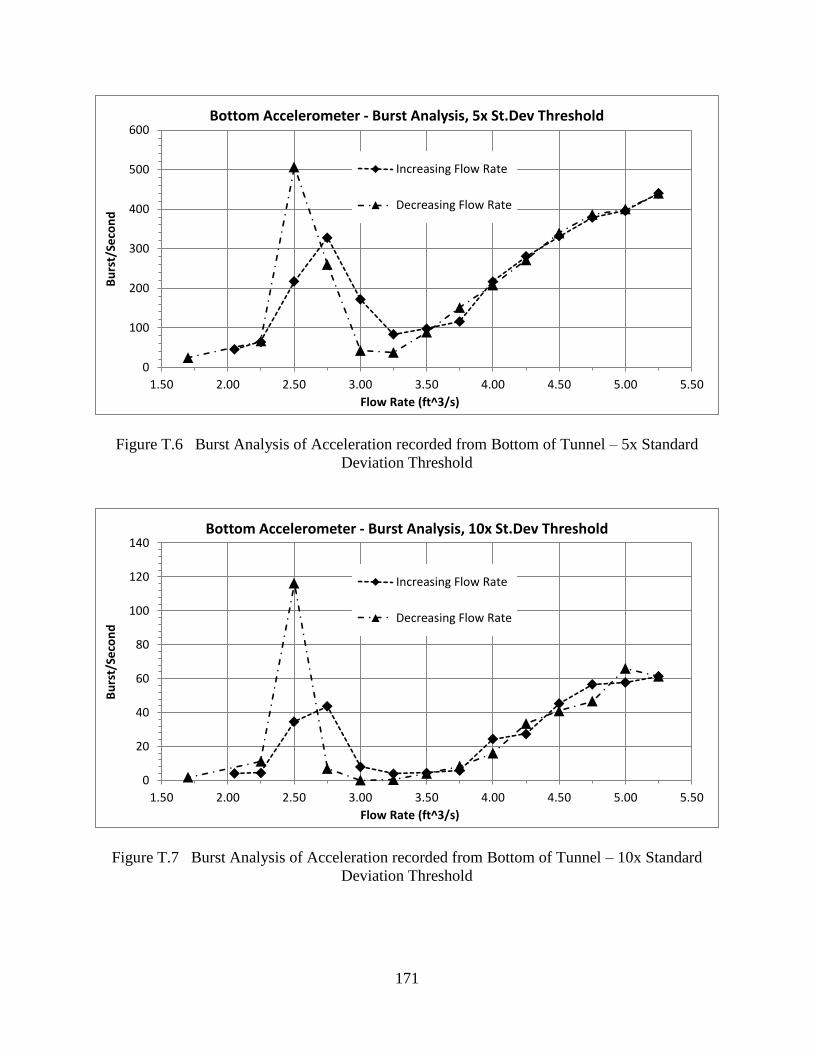
171
Figure T.6 Burst Analysis of Acceleration recorded from Bottom of Tunnel – 5x Standard
Deviation Threshold
Figure T.7 Burst Analysis of Acceleration recorded from Bottom of Tunnel – 10x Standard
Deviation Threshold
0
100
200
300
400
500
600
1.50 2.00 2.50 3.00 3.50 4.00 4.50 5.00 5.50
Bu
rst/
Seco
nd
Flow Rate (ft^3/s)
Bottom Accelerometer - Burst Analysis, 5x St.Dev Threshold
Increasing Flow Rate
Decreasing Flow Rate
0
20
40
60
80
100
120
140
1.50 2.00 2.50 3.00 3.50 4.00 4.50 5.00 5.50
Bu
rst/
Seco
nd
Flow Rate (ft^3/s)
Bottom Accelerometer - Burst Analysis, 10x St.Dev Threshold
Increasing Flow Rate
Decreasing Flow Rate
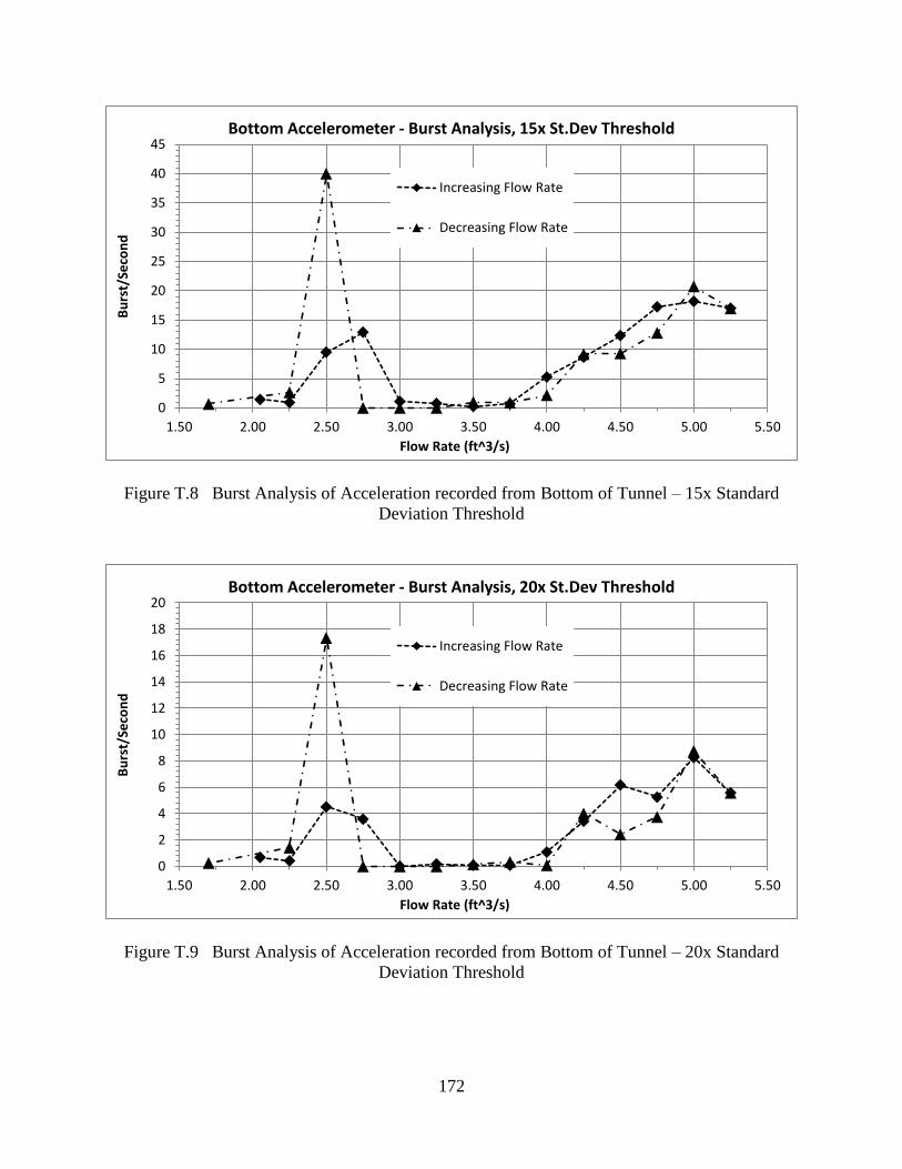
172
Figure T.8 Burst Analysis of Acceleration recorded from Bottom of Tunnel – 15x Standard
Deviation Threshold
Figure T.9 Burst Analysis of Acceleration recorded from Bottom of Tunnel – 20x Standard
Deviation Threshold
0
5
10
15
20
25
30
35
40
45
1.50 2.00 2.50 3.00 3.50 4.00 4.50 5.00 5.50
Bu
rst/
Seco
nd
Flow Rate (ft^3/s)
Bottom Accelerometer - Burst Analysis, 15x St.Dev Threshold
Increasing Flow Rate
Decreasing Flow Rate
0
2
4
6
8
10
12
14
16
18
20
1.50 2.00 2.50 3.00 3.50 4.00 4.50 5.00 5.50
Bu
rst/
Seco
nd
Flow Rate (ft^3/s)
Bottom Accelerometer - Burst Analysis, 20x St.Dev Threshold
Increasing Flow Rate
Decreasing Flow Rate
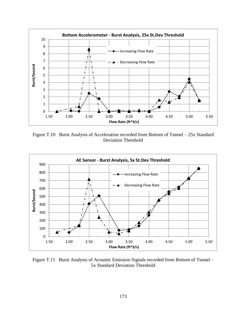
173
Figure T.10 Burst Analysis of Acceleration recorded from Bottom of Tunnel – 25x Standard
Deviation Threshold
Figure T.11 Burst Analysis of Acoustic Emission Signals recorded from Bottom of Tunnel –
5x Standard Deviation Threshold
0
1
2
3
4
5
6
7
8
9
10
1.50 2.00 2.50 3.00 3.50 4.00 4.50 5.00 5.50
Bu
rst/
Seco
nd
Flow Rate (ft^3/s)
Bottom Accelerometer - Burst Analysis, 25x St.Dev Threshold
Increasing Flow Rate
Decreasing Flow Rate
0
100
200
300
400
500
600
700
800
900
1.50 2.00 2.50 3.00 3.50 4.00 4.50 5.00 5.50
Bu
rst/
Seco
nd
Flow Rate (ft^3/s)
AE Sensor - Burst Analysis, 5x St.Dev Threshold
Increasing Flow Rate
Decreasing Flow Rate
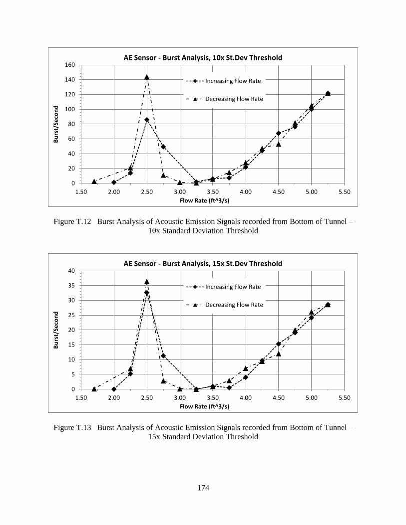
174
Figure T.12 Burst Analysis of Acoustic Emission Signals recorded from Bottom of Tunnel –
10x Standard Deviation Threshold
Figure T.13 Burst Analysis of Acoustic Emission Signals recorded from Bottom of Tunnel –
15x Standard Deviation Threshold
0
20
40
60
80
100
120
140
160
1.50 2.00 2.50 3.00 3.50 4.00 4.50 5.00 5.50
Bu
rst/
Seco
nd
Flow Rate (ft^3/s)
AE Sensor - Burst Analysis, 10x St.Dev Threshold
Increasing Flow Rate
Decreasing Flow Rate
0
5
10
15
20
25
30
35
40
1.50 2.00 2.50 3.00 3.50 4.00 4.50 5.00 5.50
Bu
rst/
Seco
nd
Flow Rate (ft^3/s)
AE Sensor - Burst Analysis, 15x St.Dev Threshold
Increasing Flow Rate
Decreasing Flow Rate
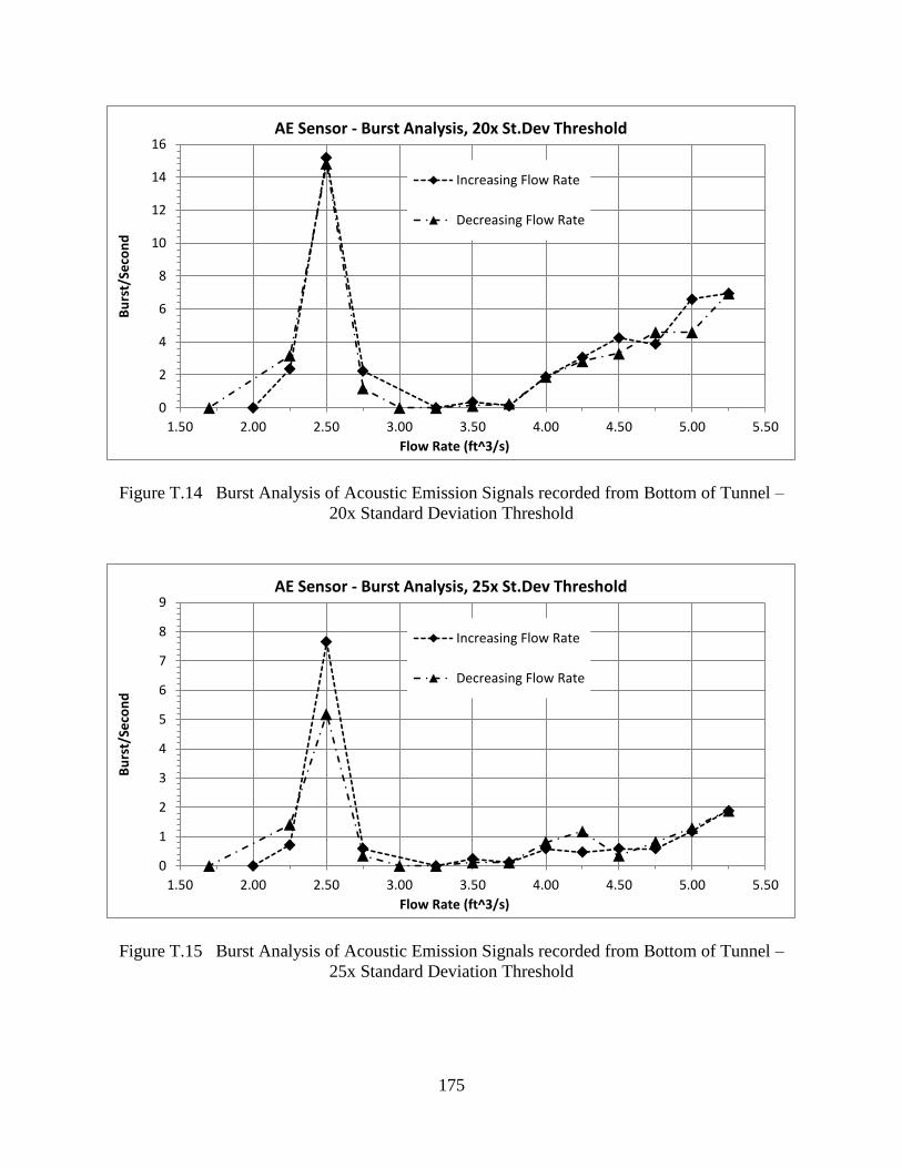
175
Figure T.14 Burst Analysis of Acoustic Emission Signals recorded from Bottom of Tunnel –
20x Standard Deviation Threshold
Figure T.15 Burst Analysis of Acoustic Emission Signals recorded from Bottom of Tunnel –
25x Standard Deviation Threshold
0
2
4
6
8
10
12
14
16
1.50 2.00 2.50 3.00 3.50 4.00 4.50 5.00 5.50
Bu
rst/
Seco
nd
Flow Rate (ft^3/s)
AE Sensor - Burst Analysis, 20x St.Dev Threshold
Increasing Flow Rate
Decreasing Flow Rate
0
1
2
3
4
5
6
7
8
9
1.50 2.00 2.50 3.00 3.50 4.00 4.50 5.00 5.50
Bu
rst/
Seco
nd
Flow Rate (ft^3/s)
AE Sensor - Burst Analysis, 25x St.Dev Threshold
Increasing Flow Rate
Decreasing Flow Rate
176
In the main body of this Thesis, the above fifteen figures were presented in a
normalized/averaged manner to compress the information into three figures. This was achieved
by normalizing all the Burst analyses by the same data point – decreasing flow rate: 2.75 ft3/s.
For the majority of the Burst analysis, this was the maximum value, hence why it was chosen.
The normalization allowed all the Burst analyses to be represented in relative terms from zero to
one. Any flow rates equal to one or close to it, represent the most volatile flow rates. Any flow
rates equal to zero or close to it represent the least volatile flow rates. Once all the Burst analysis
were normalized, the different thresholds (5x, 10x, 15x, 20x, 25x) were all averaged together.
This normalization/averaging allowed for any anomalies to be removed from the data while
maintaining the consistent trends found in all the Burst Analysis.