
Confidence sets for asset correlations in portfolio credit risk · Confidence sets for asset...
40
Revista de Econom´ ıa del Rosario. Vol. 15. No. 1. Enero - Junio 2012. 19 - 58 Confidence sets for asset correlations in portfolio credit risk Recibido: Octubre, 2011 – Aceptado: Mayo, 2012 Carlos Castro ∗ Departamento de Econom´ ıa, Universidad del Rosario. Abstract Asset correlations are of critical importance in quantifying portfolio credit risk and economic capi- tal in financial institutions. Estimation of asset correlation with rating transition data has focused on the point estimation of the correlation without giving any consideration to the uncertainty around these point estimates. In this article we use Bayesian methods to estimate a dynamic factor model for default risk using rating data (McNeil et al., 2005; McNeil and Wendin, 2007). Bayesian methods allow us to formally incorporate human judgement in the estimation of asset correlation, through the prior distribution and fully characterize a confidence set for the correla- tions. Results indicate: i) a two factor model rather than the one factor model, as proposed by the Basel II framework, better represents the historical default data. ii) importance of unobserved factors in this type of models is reinforced and point out that the levels of the implied asset cor- relations critically depend on the latent state variable used to capture the dynamics of default, as well as other assumptions on the statistical model. iii) the posterior distributions of the asset correlations show that the Basel recommended bounds, for this parameter, undermine the level of systemic risk. JEL Classification: G32, G33, C01. Keywords: Asset correlation, non-Gaussian state space models, Bayesian estimation techniques, zero-inflated binomial models. Conjuntos de confianza para la correlaci ´ on de activos en el riesgo de cr´ edito de un portafolio Resumen Las correlaciones entre los activos de un portafolio crediticio, son par´ ametros de suma impor- tancia para la estimaci ´ on del riesgo crediticio y capital econ´ omico de una instituci ´ on financiera. La literatura especializada en la estimaci ´ on de las correlaciones entre los activos, que utiliza in- formaci ´ on de migraciones entre las calificaciones de riesgo, se ha concentrado principalmente en la estimaci ´ on puntual de los par´ ametros, desconociendo la incertidumbre alrededor del esti- mador puntual. En este articulo utilizamos m´ etodos bayesianos para estimar el modelo factorial din´ amico para riesgo de quiebra utilizando datos de calificaciones de riesgo sobre un portafolio crediticio (McNeil et al., 2005; McNeil and Wendin, 2007). Los m´ etodos bayesianos nos permiten: * Autor para correpondencia. Departamento de Econom´ ıa, Universidad del Rosario, Bogot´ a, Colombia. Tel: (571) 2970200, Fax: (571) 2970200. Correo electr ´ onico: car- [email protected] c ⃝ Revista de Econom´ ıa del Rosario. Universidad del Rosario. ISSN 0123-5362 - ISSNE 2145-454x
Transcript of Confidence sets for asset correlations in portfolio credit risk · Confidence sets for asset...

Revista de Economıa del Rosario. Vol. 15. No. 1. Enero - Junio 2012. 19 - 58
Confidence sets for asset correlations in portfolio credit risk
Recibido: Octubre, 2011 – Aceptado: Mayo, 2012
Carlos Castro∗
Departamento de Economıa, Universidad del Rosario.
Abstract
Asset correlations are of critical importance in quantifying portfolio credit risk and economic capi-tal in financial institutions. Estimation of asset correlation with rating transition data has focusedon the point estimation of the correlation without giving any consideration to the uncertaintyaround these point estimates. In this article we use Bayesian methods to estimate a dynamicfactor model for default risk using rating data (McNeil et al., 2005; McNeil and Wendin, 2007).Bayesian methods allow us to formally incorporate human judgement in the estimation of assetcorrelation, through the prior distribution and fully characterize a confidence set for the correla-tions. Results indicate: i) a two factor model rather than the one factor model, as proposed bythe Basel II framework, better represents the historical default data. ii) importance of unobservedfactors in this type of models is reinforced and point out that the levels of the implied asset cor-relations critically depend on the latent state variable used to capture the dynamics of default,as well as other assumptions on the statistical model. iii) the posterior distributions of the assetcorrelations show that the Basel recommended bounds, for this parameter, undermine the levelof systemic risk.
JEL Classification: G32, G33, C01.Keywords: Asset correlation, non-Gaussian state space models, Bayesian estimation techniques,zero-inflated binomial models.
Conjuntos de confianza para la correlacion de activos en elriesgo de credito de un portafolio
Resumen
Las correlaciones entre los activos de un portafolio crediticio, son parametros de suma impor-tancia para la estimacion del riesgo crediticio y capital economico de una institucion financiera.La literatura especializada en la estimacion de las correlaciones entre los activos, que utiliza in-formacion de migraciones entre las calificaciones de riesgo, se ha concentrado principalmenteen la estimacion puntual de los parametros, desconociendo la incertidumbre alrededor del esti-mador puntual. En este articulo utilizamos metodos bayesianos para estimar el modelo factorialdinamico para riesgo de quiebra utilizando datos de calificaciones de riesgo sobre un portafoliocrediticio (McNeil et al., 2005; McNeil and Wendin, 2007). Los metodos bayesianos nos permiten:
∗Autor para correpondencia. Departamento de Economıa, Universidad del Rosario,Bogota, Colombia. Tel: (571) 2970200, Fax: (571) 2970200. Correo electronico: [email protected]
c⃝ Revista de Economıa del Rosario. Universidad del Rosario.ISSN 0123-5362 - ISSNE 2145-454x

20 Confidence sets for asset correlations
incorporar formalmente la informacion experta en el proceso de estimacion de las correlacionesmediante la distribucion a priori y obtener intervalos de confianza alrededor de los parametrosde interes. Los resultados indican: i) un modelo de dos factores se ajusta mejor a la informacionhistorica de quiebras, que el modelo de un factor (recomendado en Basilea II), ii) resalta la im-portancia de la introduccion de factores no-observables en la especificacion del modelo, en par-ticular, las propiedades estadısticas de los factores no-observables puede tener un efecto impor-tante sobre la magnitud de las correlaciones estimadas, iii) las distribuciones a posteriori de lascorrelaciones entre los activos indican que los intervalos sugeridos por el documento de Basileasubestiman el riesgo sistemico.
Clasificacion JEL: G32, G33, C01.Palabras clave: Correlacion de activos, modelos espacio estado no gausianos, tencicas de esti-macion bayesiana, modelo binomial con inflacion cero.
Revista de Economıa del Rosario. Vol. 15. No. 1. Enero - Junio 2012. 19 - 58
Castro 21
1 Introduction
Asset dependence in portfolio credit risk management is a topic of growingimportance for practitioners and academics. Changes in the most commonform of dependence (correlation) across assets transfer some of the risk fromthe mean towards the tail of the loss distribution. Any increase in correlationbetween the assets fattens the tail of the loss distribution and therefore re-quires a greater amount of capital set aside to cover unexpected losses. Henceasset correlation is a cornerstone parameter in the estimation of a bank’s cap-ital requirements. Tarashev et al. (2007) show that misspecified or incorrectlycalibrated correlations can lead to significant inaccuracies in the measures ofportfolio credit risk and economic capital.
The Basel accord of 1988 was a first attempt to establish an internationalstandard on a bank’s capital requirements. However a significant drawbackwas the accord’s crude approach to determine the risk weights assigned todifferent positions in a bank’s portfolio. For example, a private firm witha top rating would receive a weight a hundred times higher than any typeof sovereign debt, regardless of the rating of the former. The second Basel(henceforth Basel II) corrected the imbalance by accounting for the relativecredit quality of the issuers.1 Under Basel II regulators gave more leeway tobanks with the hope that they are able to perform a more accurate measure ofthe risk heterogeneity of their portfolio. Hence bank managers have greaterfreedom to calibrate the assigned risk weights and derive more accurate lossdistributions for their portfolios.
In general, techniques to derive the loss distribution for the portfolio re-quire simulation. Considering the dependence across all individual nameswould be very cumbersome, hence factor models provide simple ways to mapthe dependence structure in the portfolio. Under the internal-rating-based(IRB) approach to determine the risk weights, proposed in Basel II, the un-derlying structure behind default dependence is a one factor model. Basel IIsuggests a value for the correlation parameter, the unique dependence param-eter of this one factor model, between 0.12 and 0.24. The literature proposesvarious estimates for these values in the ranges (0.01-0.1) Chernih et al. (2006)and (0.05-0.21) Akhavein et al. (2005).
The risk factor model, used extensively in the literature on dynamic mod-eling of default risk, provides the structure to estimate asset correlations withrating data. This model decomposes credit risk into systematic (macro re-lated) and idiosyncratic (issuer specific) components. In this context (McNeilet al., 2005; McNeil and Wendin, 2007) and Koopman and Lucas (2008) pro-vide estimation methods to fit the dynamics of default. The former exploresheterogeneity among industry sectors and also across rating classes whereasthe later only explores heterogeneity across ratings. Both articles recognizetwo difficulties inherent to rating data and, particularly, default: i) rating tran-sitions are scarce events and ii) defaults are extremely rare events. These two
1The recommendations from the Basel II accord are contained in a document published bythe Basel Committee on banking supervision (2006).
Revista de Economıa del Rosario. Vol. 15. No. 1. Enero - Junio 2012. 19 - 58

22 Confidence sets for asset correlations
elements make statistical inference more difficult. However, rating transitiondata is a preferred proxy for changes in the creditworthiness of issuers be-cause it is more direct than using other proxies such as equity or spread data.Moreover, equity based correlation is not readily available for some types ofissuers. For example, for sovereigns and structured products there is no infor-mation available for equity or debt. Therefore, it is not possible to link equityand assets through the option-theoretic framework due to Merton (1974).
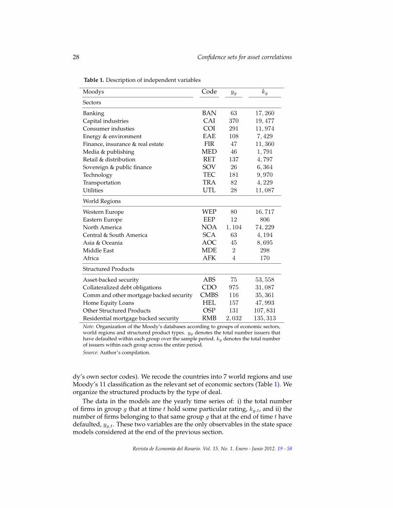
The aim of this article is twofold: First, estimate asset correlations withinand across different identifiable forms of grouping the issuers. Second, pro-vide a sensibility analysis of these estimates with respect to the model as-sumptions. We use Moody’s rating data for Corporate defaults and Structuredproducts. The Corporate default database contains information on 51,542 rat-ing actions affecting 12,292 corporate and financial institutions during the pe-riod 1970 to 2009. The Structured products database contains information on377,005 rating actions affecting 134,554 structured products during the period1981 to 2009. The database contains information on group affiliation of theissuers such as type of product, or economic sector and country where a firmcarries out its business.2 According to the group affiliation, firms are orga-nized into 11 sectors, 7 world regions and 6 structured products (Table 1).
The disaggregated approach (first objective), with respect to a world aggre-gate, contributes to the existing literature on asset correlation since most of theliterature has focused on estimating these models on aggregate data (in partic-ular aggregate US default count). With respect to world region affiliation andstructured products, the results in this article are a novelty. Furthermore, if ac-counting for heterogeneity in a bank’s portfolio is an important part of BaselII, it is senseless estimating models based on the aggregated data. By mov-ing away from the aggregated data, the few historical observations that areavailable on rating transitions (especially default) become even more sparse.Therefore the existing methodologies encounter problems due to the sparsityof the data.
The sensibility of the estimates of asset correlation with respect to themodel assumptions (second objectives) goes beyond the Basel II benchmark:the one factor model. The elements of the model that are analyzed, with re-gard to their effect over the parameters of interests, are the following: i) in-troduction of additional group specific factors (i.e. a two factor model), ii) thenature for the factors (i.e. observed or unobserved), iii) the data generatingprocess of the factors, iv) the functional form of the default probability (i.e.probit or logit), and v) for a given rating system, the implications of migratingfrom different ratings to default (i.e. correlation asymmetry).
We use a generalized linear mixed model (GLMM hereafter) for estima-tion. This model considers the observed number of firms that perform somemigration (possibly to the default state), out of a total number of firms within
2The main unit of analysis throughout the paper is an issued financial obligation that hassome particular rating. The financial obligation can take many forms: On one hand it can be acorporate bond, issued by a firm. On the other hand it can also be a financial product such as astructured product. Therefore, it is important to note that when we refer to firms or issuers, weimplicitly refer to the entity which is liable for such financial obligations.
Revista de Economıa del Rosario. Vol. 15. No. 1. Enero - Junio 2012. 19 - 58
Castro 23
a given group (say an economic sector or world region), as a realization of abinomial distribution conditional on the state of some unobserved systematicfactor. A one or two factor model (1-F, 2-F, henceforth) allows the decompo-sition of default risk into the estimated factor(s) and the idiosyncratic compo-nent. A set of identifying assumptions on the model allows for the estimationof both the factor(s) and the factor(s) loading(s). The state space model builtfrom this setup has a measurement equation that has the form of a binomialdistribution (making the model non-Gaussian and non-linear).
We find that the loading parameters of the factors across the 11 sectors,7 world regions and 6 structured products are in general statistically signifi-cant. We recover the asset correlations from the factor loadings and observethat in some cases, the asset correlations are higher than the Basel II recom-mended values. For most models there is even a null or very small probabilitythat the asset correlation parameter is within the bounds recommended in theBasel II document. Asset correlation is in particular very sensitive to the as-sumptions of the statistical model; for instance if the unobserved componentis autoregressive, as opposed to i.i.d.. Moreover, the two factor model withAR(1) dynamics for the global factor and with a local systemic factor (called itsectorial, regional, or product) is able to reproduce better the observed num-ber of defaults than the 1-F framework recommended by Basel II.
The results have two direct implications on the measurement of economiccapital. First, they show that the one factor model is too restrictive to accountin a proper manner for the dependence structure in the data and hence theportfolio. A two factor model provides a hierarchical structure to the banksportfolio while still being parsimonious in terms of the parameters. Thismodel includes a global systemic factor plus a local systemic factor in addi-tion to the idiosyncratic component. The set of local systemic factors accountfor significant difference across identifiable grouping characteristic within theportfolio such as economic sectors and world regions. Second the estimates ofthe dependent structure are strongly reliant on modeling assumptions, hencethey convey significant model risk. This source of model risk should be takeninto account in the process of model validation by the regulators.
The outline of the paper is as follows: Section 2 presents the dynamic de-fault risk model. Section 3 describes the data. Section 4 presents the estimationmethods, the results and the implications on the estimation of economic capi-tal. Sections 5 provides methodological solution to the common data scarcityproblem found in default models. Section 6 concludes.
2 Dynamic factor model of default risk
The default risk model has its roots in the work by Merton (1974). In the last10 years this model has been at the center of the literature on portfolio creditrisk modeling. The most general version of the Merton model considers theasset value of a firm i = 1, .., N at time t = 1, .., T , Vi,t as a latent stochasticvariable. Let Vi,t follow a standard normal distribution. If Vi,t falls below apredetermined threshold µi,t (related to the level of debt) then a particular
Revista de Economıa del Rosario. Vol. 15. No. 1. Enero - Junio 2012. 19 - 58
24 Confidence sets for asset correlations
event is triggered. This event refers to a transition between states defined un-der some rating system. For capital adequacy purposes, the most importantevent is default. However, since historically this is a rare event, it is also inter-esting to consider a larger state-space to account for all possible transition in agiven rating system.3 These firms belong to the portfolio of an investor (say abank) that wishes to model the default dependence across the portfolio. Withthis in mind, the investor considers a F-factor model (F-F, henceforth) as theunderlying structure behind the dynamics and dependence structure of theasset value for the firms that belong in the portfolio:
Vi,t :=
F∑f=1
af,iBf,t +
√√√√1−F∑f=1
a2f,iei,t,∀t ∈ T. (1)
In equation (1) the asset value of the firm is driven by F common factors Bf,t(common to all firms) and a firm-idiosyncratic component, ei,t (Demey et al.,2004). Let Bt = (B1,t, ..., BF,t) and et = (e1,t, ..., eN,t) be two F × 1 andN × 1 vector of factors and idiosyncratic components. We assume that bothcomponents follow a multivariate normal distribution, Bt ∼ N(0, IF ), et ∼N(0, IN ), and are orthogonal to each other, E[ei,t, Bj,s] = 0 ∀t, s, i = j. Theelements af,i make up the factor loading matrix A (of dimension N × F ). Theweighting scheme of the F-F model along with the distributional assumptionson the factors and idiosyncratic components guarantees that the asset valuesare standard normally distributed. Furthermore, under these conditions, theentire dependent structure is determined by AA′ = Σ (a N ×N matrix).
Although the model is indexed for a particular firm, in practice estimationof the parameters is performed on a more aggregate scale. If the parametersare indexed at the firm level then there are a total ofN(N+1)/2 parameters toestimate the dependence structure. This model is therefore computationallyexpensive for a large set of firms. One way to reduce dimensionality is todefine a set of homogeneous risk classes, i.e. group firms by some identifiablecharacteristic, economic sector or the world region they belong to. Note g =1, . . . , G as group indicator where G << N (much smaller that N ), with thefollowing implications for the model parameters:
1. Default threshold is unique within each group and across time, µi,t = µg∀i ∈ g.
2. Constant correlation between firms in same group, ρi,j = ρg ∀i, j ∈ g.3. Unique correlation between firms in different groups, ρi,j = ρg,d ∀i ∈g, j ∈ d.
These assumptions imply a symmetric G×G correlation matrix Σ
Σ =
ρ1 ρ1,2 . . . ρ1,G
ρ1,2 ρ2. . .
......
. . . . . . ρG−1,G
ρ1,G . . . ρG−1,G ρG
.
3An example of a rating system is Moody’s ratings on long term obligations (broad version):Aaa, Aa, A, Baa (investment grade), Ba, B, Caa, Ca, C(speculative grade or non-investment grade).
Revista de Economıa del Rosario. Vol. 15. No. 1. Enero - Junio 2012. 19 - 58

Castro 25
With the previous assumptions and if Σ is positive and definite, the F-factormodel with G(G+ 1)/2 parameters is:
Vi,t :=
F∑f=1
af,gBf,t +√1− ρgei,t, ∀i ∈ g. (2)
We introduce an additional restriction so as to further reduce the param-eter space to G + 1 correlations. This restriction implies that the correlationamong two groups is unique among all the groups, ρg,d = ρ ∀g = d, whichimplies
Σ =
ρ1 ρ . . . ρ
ρ ρ2. . .
......
. . . . . . ρρ . . . ρ ρG
.
where ρ denoted inter correlation and ρi j = 1, ..., G intra correlations. We canbe show that this new dependence structure is equivalent to the dependencestructure derived from a 2-factor model (2-F, henceforth), instead of the F-Fmodel:
Vi,t :=√ρBt +
√ρg − ρBg,t +
√1− ρgei,t, ∀i ∈ g, (3)
where Bt represents a global systemic factor and Bt,g represent a local sys-temic factors that determines the default process.
One further restriction is possible so that there is only one relevant riskclass: ρg = ρ , hence the model reduces to a 1-factor model (1-F, henceforth)
Vi,t :=√ρBt +
√1− ρei,t∀i. (4)
In this case, the dependence structure across a set of firms (in the bank’s port-folio) is determined entirely by the parameter ρ. This model reflects the BaselII framework and considered to be an oversimplified representation of the fac-tor structure underlying default dependence, particularly for internationallyactive banks (McNeil et al., 2005). The main pitfall of the 1-F approach is thatit does not detect concentrations or recognize diversification (the dependencestructure of the whole portfolio is described by one parameter).
Once a particular dynamic structure for the asset value Vi,t is chosen assatisfactory (F-F, 2-F, or 1-F), the next step is to link this setup to the observedrating transitions in order to estimate the parameters of interest i.e., the ele-ments of the Σ matrix. The rating information on the firms, such as the oneprovided by Moodys, provides the count data to characterize default risk interms of the number of firms that went into default for a particular period. Letkg,t be the number of firms in group g at time t, and yg,t the number of firmsthat made some transition between the two states (non-default and default)between t and t+ 1. We assume that the number of defaults are conditionallyindependent across time given the realization of the latent factors. Then yg,thas the following conditional distribution
yg,t|Bt ∼ Binomial(kg,t, πg,t), g = 1, .., G; t = 1, .., T, (5)
Revista de Economıa del Rosario. Vol. 15. No. 1. Enero - Junio 2012. 19 - 58
26 Confidence sets for asset correlations
where πg,t is the conditional probability of default and Bt = (Bt, B1,t, . . . , BG,t)is the vector of global and local systemic factors. Equation (3) constitutes themeasurement equation of a state space model.
As mentioned previously, default occurs if the asset value of the firm Vi,tfalls bellow threshold µg,t. Therefore, this probability can be expressed asa probability function P : R → (0, 1), depending on the threshold and thedynamics (F-F, 2-F, 1-F) that describe the evolution of the asset value of thefirms that belong to the portfolio:
πg,t = P (Vi,t ≤ µg | Bt)
= P
(ei,t ≤
µg −√ρBt −
√ρg − ρBg,t√
1− ρg
)
= Φ
(µg −
√ρBt −
√ρg − ρBg,t√
1− ρg
).
The factors are the main drivers of the credit conditions, often considered as aproxies for the credit cycle, Koopman et al. (2009). We consider multiple dy-namics for the unobserved factors (autoregressive, random walk, white noise).For now assume that the factor(s) follow an VAR(1) process:
Bt = ΨBt−1 +Θηt, (6)
where ηt ∼ N(0, I), and Ψ = diag(ψ,ψ1, . . . , ψG),Θ = diag(
√1− ψ2,
√1− ψ2
1 , . . . ,√1− ψ2
G). The weighting scheme of theVAR(1) process guarantees that each factor is standardized (Bg,t ∼ N(0, 1)),as required. This normalization of the factors is important in order to be able
to identify the loading parameters (√ρ√
1−ρg,
√ρg−ρ√1−ρg
) and the parameters of in-
terest the implied correlations (ρ, ρg). Equation 6 constitutes the state equationof a state-space model.
In the portfolio credit risk literature various authors (Gordy and Heitfield,2002; Demey et al., 2004; Koopman and Lucas, 2008; Wendin and McNeil,2006; McNeil and Wendin, 2007) propose similar types of factor models fordefault risk, the so called structural type models that follow the Mertonianframework. All the underlying models, as well a the model proposed in ex-pressions 5 and 6, are special cases of the generalized linear mixed model(GLMM) for portfolio credit risk, see Wendin (2006).
There are two considerations that border on the theoretical and the em-pirical with respect to the factors, (Bt), that make up the state equation ofthe model 6. The first issue is whether the factor(s) in the default risk modelshould be considered as unobserved, observed or both. The factor(s) repre-sent the main driver (systemic component) behind the possibility that a firmgoes into default or not. Systematic credit risk factors are usually consideredto be correlated with macroeconomic conditions. Nickell et al. (2000), Bangiaet al. (2002) Kavvathas (2001), and Pesaran et al. (2006) use macroeconomicvariables as factors in default risk models. However, there are some doubts
Revista de Economıa del Rosario. Vol. 15. No. 1. Enero - Junio 2012. 19 - 58

Castro 27
whether there is an adequate alignment between the credit cycle (implied byrating and default data) and the macroeconomic variables. Koopman et al.(2009) indeed show that business cycle, bank lending conditions, and finan-cial market variables have low explanatory power with respect to default andrating dynamic. Das et al. (2007) find that US corporate default rates between1979 and 2004 vary beyond what can be explained by a model that only in-cludes observable covariates. Such results give a strong motivation for theintroduction of unobserved components in default risk models. Furthermore,Wendin and McNeil (2006); McNeil and Wendin (2007) and Koopman and Lu-cas (2008) show that there are gains in term of the fit of the model and forecast-ing accuracy, when both observed macroeconomic covariates and unobservedcomponents are considered.
The last issue is the dynamic characterization of the factors. In some of theearliest articles that focus on the estimation of asset correlations, the factorswere considered as (i.i.d.) standard normal random variables.4 However, Ban-gia et al. (2002) and Nickell et al. (2000) have empirically shown that changesin the macroeconomic environment have some effect over rating transitionsand default, which suggest that the credit default process is serially correlated.Furthermore, the source of this serial correlation is the autocorrelation presentin the factor (observed macro covariates and/or the unobserved component).The existence of serial correlation also points to the fact that rating procedureswithin the rating agencies are more through-the-cycle than point-in-time.
3 Data and Stylized Facts
3.1 Data
We use Moody’s Corporate Default database on issuer senior rating, whichcontains information on 51,542 rating actions affecting 12,292 corporate andfinancial institutions during the period 1970 to 2009. 5 We also use Moody’sdatabase on Structured Products that contains information on 377,005 ratingactions affecting 134,554 structured products (only the super senior trench)during the period 1981 to 2009.
Moody’s database considers 9 broad ratings (Aaa, Aa,..) for the period1970 to 1982 and 18 alphanumeric ratings (Aaa, Aa1, Aa2,..) from 1983 on-wards. For consistency the 9 broad ratings are considered throughout thesample. Although Moody’s does not have an explicit default state, it doeshave a flag variable that indicates when an issuer can be considered in defaultor close to it. Since there are different definitions of default (e.g. missed ordelayed disbursement of interest and/or principal, bankruptcy, distressed ex-change) Moody’s keeps rating the issuer according to their rating grades. Weuse the flag variable to determine a unique date of default irrespective of thefact that Moody’s still gives a broad grade.
Additional to the rating information for each issuer there is an assignedcountry and economic sector codes (two and four digits SIC codes and Moo-
4See Gordy and Heitfield (2002) and Demey et al. (2004).5The last observation in the database is April 2009.
Revista de Economıa del Rosario. Vol. 15. No. 1. Enero - Junio 2012. 19 - 58
28 Confidence sets for asset correlations
Table 1. Description of independent variables
Moodys Code yg kg
Sectors
Banking BAN 63 17, 260Capital industries CAI 370 19, 477Consumer industies COI 291 11, 974Energy & environment EAE 108 7, 429Finance, insurance & real estate FIR 47 11, 360Media & publishing MED 46 1, 791Retail & distribution RET 137 4, 797Sovereign & public finance SOV 26 6, 364Technology TEC 181 9, 970Transportation TRA 82 4, 229Utilities UTL 28 11, 087
World Regions
Western Europe WEP 80 16, 717Eastern Europe EEP 12 806North America NOA 1, 104 74, 229Central & South America SCA 63 4, 194Asia & Oceania AOC 45 8, 695Middle East MDE 2 298Africa AFK 4 170
Structured Products
Asset-backed security ABS 75 53, 558Collateralized debt obligations CDO 975 31, 087Comm and other mortgage backed security CMBS 116 35, 361Home Equity Loans HEL 157 47, 993Other Structured Products OSP 131 107, 831Residential mortgage backed security RMB 2, 032 135, 313Note: Organization of the Moody’s databases according to groups of economic sectors,world regions and structured product types. yg denotes the total number issuers thathave defaulted within each group over the sample period. kg denotes the total numberof issuers within each group across the entire period.Source: Author’s compilation.
dy’s own sector codes). We recode the countries into 7 world regions and useMoody’s 11 classification as the relevant set of economic sectors (Table 1). Weorganize the structured products by the type of deal.
The data in the models are the yearly time series of: i) the total numberof firms in group g that at time t hold some particular rating, kg,t, and ii) thenumber of firms belonging to that same group g that at the end of time t havedefaulted, yg,t. These two variables are the only observables in the state spacemodels considered at the end of the previous section.
Revista de Economıa del Rosario. Vol. 15. No. 1. Enero - Junio 2012. 19 - 58

Castro 29
As mentioned previously, the event of default is an extremely rare event,inference on this type of event is complex. In particular the time series ofdefaults suffer of overdispersion or zero-inflation. This zero inflation is exac-erbated when we disaggregate the data into groups (i.e. sectors, regions andproducts). Since default is already a rare event in the aggregate, then when wemake a subgroup of this aggregate, the observed defaults become even fewerwithin each group. The problem of zero-inflation affects the model since it de-viates from the assumption that the default counts have a binomial behavior.In other words, an increasing number of zeros may degenerate the distribu-tion. In order to overcome the problems due to overdispersion, a zero-inflatedbinomial model for the default counts is developed and estimated in Section5.
3.2 Stylized Facts
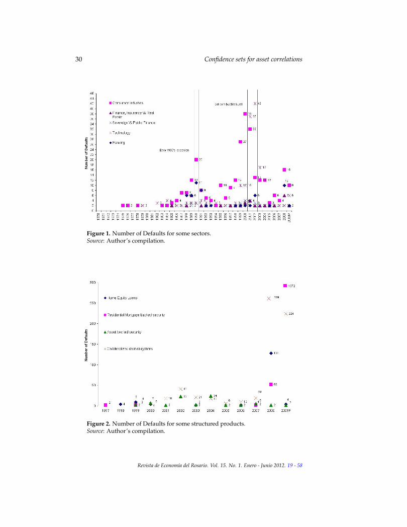
The database on long term corporate issuers is to a great extend (especially inthe first part of the sample) composed of US issuers. The US data representsabout 65% of the potential data on rating transitions. Figures 1 illustratesthe number of defaults for five sectors, consumer industries, and technology,which have a significant number of defaults, banking, finance/insurance/realestate and sovereign/public finance, which have few rating movements. Thelater illustrates the problem of zero-inflation. Consumer industries have animportant participation on defaults throughout all the sample, while technol-ogy is a late starter and shows increasing activity in 2002 and 2001, whichwas a very volatile period for the industry (the burst of the telecommunica-tions bubble that had its peak in the late 2000). Although sectors are believedto show their own dynamics, there are periods of general turmoil (clusteringeffects) that are evident in the sample, especially at the end of the nineties.
For structured products (Figure 2), the information available has increasedwith the rapid expansion of the market for these types of securities. Mostof the relevant information is at the end of the sample. It is also evident theincreasing number of defaults in 2008 and the preliminary data of 2009, espe-cially in collateralized debt obligations and residential mortgage backed secu-rities.
In general the figures on sectors and structures products show a great dealof heterogeneity in default events. In the estimation part, the objective is to tryto capture the intra and inter correlations due to rating movements. Further-more, since rating movements are closely related to creditworthiness, resultswill give some idea of the asset correlations.
Revista de Economıa del Rosario. Vol. 15. No. 1. Enero - Junio 2012. 19 - 58
30 Confidence sets for asset correlations
Figure 1. Number of Defaults for some sectors.Source: Author’s compilation.
Figure 2. Number of Defaults for some structured products.Source: Author’s compilation.
Revista de Economıa del Rosario. Vol. 15. No. 1. Enero - Junio 2012. 19 - 58

Castro 31
4 Estimation
The model in section 3 is a non-linear and non-Gaussian state space modelbecause of the binomial form of the measurement equation. Furthermore themodel incorporates an unobserved component. In this context, standard lin-ear estimation techniques are not appropriate. The estimation of such model,has been performed on credit rating data, either using a Monte Carlo maxi-mum likelihood method (Koopman and Lucas, 2008; Durbin and Koopman,1997) or using Bayesian estimation, in particular Gibbs sampling (Wendin,2006; McNeil et al., 2005; McNeil and Wendin, 2007). This article follows thesecond approach mainly on two accounts: it provides greater flexibility indealing with the over dispersion (zero-inflation) and, it is possible to derive adistribution for the asset correlations (parameter of interest).
Denote ψ := (ψ1, . . . , ψG) as the relevant set of parameters. This set nat-urally includes the unobserved components. Bayesian inference considersthe unknown parameters ψ as random variables with some prior distribu-tion P (ψ). The prior distribution along with the conditional likelihood of theobserved data x := (yg,t, kg,t)G,Tg=1,t=1 are used to derived the posterior dis-tribution for the unknown parameter: P (ψ | x) ∝ P (x | ψ)P (ψ). In somecases the posterior distribution is unattainable analytically. Hence the eval-uation of the joint posterior requires the use of Markov chain Monte Carlo(MCMC) algorithms, such as the Gibbs sampler. The Gibbs sampler is a spe-cific componentwise Metropolis-Hastings algorithm that performs sequentialupdating of the full conditional distributions of the parameters in order toreproduce the joint posterior of the parameters. In other words, the algo-rithm proceeds by updating each parameter ψj by sampling from its respec-tive conditional distribution, given the current values for all other parametersψ−j := (ψ1, .., ψj − 1, ψj + 1, .., ψJ ) and the data. This conditional distributionis the so-called full conditional distribution (see appendix). With a sufficientlylarge number of repetitions, it can be shown that, under mild conditions, theupdated values represent a sample from the joint posterior distribution.
Each model is estimated using three parallel Markov chains that are initi-ated with different starting values. Convergence of the Gibbs sampler is as-sessed using the Gelman and Rubin (1992, 1996) scale-reduction factors. Theautocorrelations of sample values are also checked to verify that the chainsmix well. Only after convergence, the Deviance Information Criterion (DIC)is used to choose among the different models fitted to the data, followingSpiegelhalter et al. (2002). The different model characterize different assump-tions for the dynamic factor model for default risk (e.g. 1-F vs 2-F, dynamics ofunobserved factors). This criterion resembles the Akaike’s Information Crite-ria, since it is expected to choose the model which has the best out-of-samplepredictive power.6 The DIC is defined as follows. First recall the usual defini-tion of the deviance, dev = −2logP (x | ψ). Let dev denote the posterior meanof the deviance and dev the point estimate of the deviance computed by sub-
6The estimation was performed using WINBUGS Release version 1.4.3, http://www.mrc-bsu.cam.ac.uk/bugs/winbugs/contents.shtml.
Revista de Economıa del Rosario. Vol. 15. No. 1. Enero - Junio 2012. 19 - 58

32 Confidence sets for asset correlations
stituting the posterior mean of ψ. Thus dev = −2logP (x | ψ). Denote by pDthe effective number of parameters (elusive quantity in Bayesian inference)defined as the difference between the posterior mean of the deviance and thedeviance of the posterior means, pD = dev − dev. The DIC is defined as fol-lows: DIC = dev + pD. The model with the smallest DIC value is consideredto be the model that would predict a dataset of the same structure as the dataactually observed. Since the distribution of the DIC is unknown (no formalhypothesis testing can be done) it is a difficult task to define what constitutesan important difference in DIC values. Spiegelhalter et al. (2002) propose thefollowing rule of thumb: if the difference in DIC is greater than 10, then themodel with the larger DIC value has considerable less support than the modelwith the smallest DIC value.
As mentioned previously, a further advantage of using a full Bayesian ap-proximation is that the parameters of interest, the asset correlations, and es-pecially the uncertainty about them can be directly obtained from the MCMC.The parameters of the statistical model are the factor loadings, but we knowthat through a series of identifying restrictions in the economic model, we canestablish a functional relationship between the factor loadings and the assetcorrelations. We can include such function in the Monte Carlo procedure soas to derive directly the parameters of interest and, in particular, derive a con-fidence set for the implied correlations.
An informative prior is used for the autoregressive coefficient that deter-mines the dynamics of the unobserved factor, ψ ∼ U(−1, 1). According tothis prior the unobserved factor follows a stationary AR(1) process. Diffusebut proper priors are considered for all other parameters (the factor loadings√ρg−ρ√1−ρg
∼ U(0, 10), and the default threshold µg ∼ N(0, 103)), however other
priors are also possible if specific prior information is available for some pa-rameters.78 The sampling method used for the distributions is a Slice sampler.The sampler was run for 10,000 iterations, with the first 5,000 iterations dis-carded as a burn-in period.
The aggregate data only has a one factor representation (4), which we de-note as Model A in the tables. In such one factor representation the unob-served factor Bt has two possible dynamics a stationary and univariate AR(1)process or a white noise,i.i.d. N(0, 1).
Models which we denote B, C and D, in the tables, are based in the panelstructure for sectors, regions or structured products. These models have botha one or two factor representation (4, 3). In the two factor representation, thesecond factor can be thought as a local systemic factor.
The main difference between models C and D is that in the former the firstfactor Bt ∼ N(0, 1) is a stationary AR(1) process. This factor represents theso-called global systemic factor. The second factor of each of the groups is a
7This range for the factor loading captures all the possible values for the asset correlationρ ∈ (0, 1). Larger interval values, such as an improper prior like U(−200, 200) or N(0, 103) onlyimprove decimal point accuracy. The value is also restricted to be positive in order to preventlabel switching.
8See Tarashev et al. (2007) for some possible informative priors for the some of the parameters.
Revista de Economıa del Rosario. Vol. 15. No. 1. Enero - Junio 2012. 19 - 58
Castro 33
white noise Bt,g ∼ iidN(0, 1) ∀g. Note that this second factor represents thelocal systemic factor and is drawn from a distribution that is unique across allof the groups; whereas in Model D all of the factors are considered to be whitenoise, therefore the state equation is uniquely determined by the followingexpression Bt = ηt. It is important to note that in every case the unobservedfactors are orthonormal, guaranteeing that the factor(s) loading(s) are identi-fied.
4.1 Results
With the aggregate default data from the US, we estimate model A. The valueof the persistence parameter ϕ of the AR(1) specification is 0.91 and indicates astrong persistence, as found by Koopman and Lucas (2008), whereas Wendinand McNeil (2006) find smaller values 0.68.9 The value of the loading param-eter is 0.56 and it is close to the estimate obtained for the same specificationby Koopman and Lucas (2008). The value of the parameter gives an estimatefor asset correlation of 0.24. In general, the estimated parameters are veryclose to those obtained from a similar set up by Koopman and Lucas (2008).If the unobserved component is assumed to be i.i.d. the asset correlation fallsto 0.10. The information criteria, DIC, indicates no significant difference withrespect to the response function. Furthermore, the model with an AR(1) typeunobserved factor performs better than the i.i.d. according to the informationcriteria.10 Both the AR(1) specification as well as the i.i.d. for the unobservedcomponent provide an adequate fit to the aggregate US default data.
Correlation asymmetry is a phenomenon found consistently in the liter-ature irrespective of the data or methodology used in obtaining estimates ofasset dependence with defaults (Das and Gengb, 2004). This phenomenon hasa further intuitive appeal since it indicates that high graded issuers (in manycases large firms) have a larger exposure to systemic risk, whereas low gradedissuers (medium and small firms) face more idiosyncratic risk. Using the ag-gregate data for all world regions (not only US) the estimated asset correla-tions, from model A for the AR(1) and i.i.d. specifications for the unobservedcomponent are 0.18 and 0.09, respectably (Figure 3).
Three separate exercises were also considered using model A. The firstonly considers defaults from non-investment grade issuers. The second onlyconsiders defaults from investment grade issuers (Table 2). Results are consis-tent with correlation asymmetry, as they indicate an inverse relation betweencorrelation and the quality of the issuer. In other words correlation is larger forinvestment grade issuers (ρIG = 0.4) than for non-investment grade issuers(ρNIG = 0.17) issuers (Figure 3).
9The majority of the Moody’s data comes from the US specially the data before 1990.10Higher order autoregressive process of the unobserved factor were tested at some point but
provide no improvement over the AR(1). Results are available under request.
Revista de Economıa del Rosario. Vol. 15. No. 1. Enero - Junio 2012. 19 - 58

34 Confidence sets for asset correlations
Tabl
e2.
Esti
mat
ion
Res
ults
from
the
Agg
rega
teC
orpo
rate
defa
ultd
ata
from
1970
to20
09.
Non
-Def
ault
toD
efau
ltN
on-I
nves
tmen
tGra
deto
Def
ault
Inve
stm
entG
rade
toD
efau
lt
Mod
elA
AR
(1)
Mod
elA
i.i.d
.M
odel
AA
R(1
)M
odel
Ai.i
.d.
Mod
elA
AR
(1)
Mod
elA
i.i.d
.
Load
ings
0.45
93b
0.31
23a
0.45
58b
0.30
54a
0.82
91a
0.74
8a
(0.1
83)
(0.3
12)
(0.2
02)
(0.0
446)
(0.1
26)
(0.1
48)
ψ0.
8743
a0.
8459
a0.
7085
a
(0.8
74)
(0.1
06)
(0.1
26)
DIC
160
257
164
254
9610
0
Ass
etC
orre
lati
ons
2.5
0.05
30.
057
0.05
00.
051
0.22
30.
166
Mea
n0.
178
0.09
00.
177
0.08
60.
404
0.35
697
.50.
450
0.13
80.
472
0.14
50.
497
0.49
2N
ote:
The
resu
lts
are
first
take
nw
ith
resp
ectt
oal
lrat
edfir
ms,
seco
ndon
lyta
king
non-
inve
stm
entg
rade
rate
dfir
ms
and
last
only
taki
ngin
vest
men
tgra
dera
ted
firm
s.R
esul
tsar
epr
esen
ted
only
for
the
Prob
itre
spon
sefu
ncti
on.T
heM
onte
Car
lost
anda
rder
rors
ofth
em
ean
are
show
nin
pare
nthe
ses.
c,b
,and
ade
note
sign
ifica
nce
atth
e10%
,5%
,and
1%
leve
ls,r
espe
ctiv
ely.
Sour
ce:A
utho
r’s
esti
mat
ion.
Revista de Economıa del Rosario. Vol. 15. No. 1. Enero - Junio 2012. 19 - 58

Castro 35
The last exercise based on the model A, provides a simplified approachto capture the effects of tail risk. Since model A is a 1-F model tail risk isnaively introduced by changing the standard assumption on the distributionof the unobserved factor.11 The unobserved factor, for the sole purpose of thisexercise, follows a standardized Student-t distribution with two degrees offreedom, Bt ∼ iid t(0, 1, 2). The results indicate no significant gain with re-spect to the standard assumptions on the dynamics of the unobserved factor,according to DIC. However, the estimated value for the correlation is approx-imately half the value obtained when using the standard assumptions on thedynamics of the unobserved factor. These results imply that by considering adistribution with thicker tails than the standard Gaussian, this model is ableto capture the same default dynamics as the standard model, requiring onaverage a smaller estimate of the asset correlation.
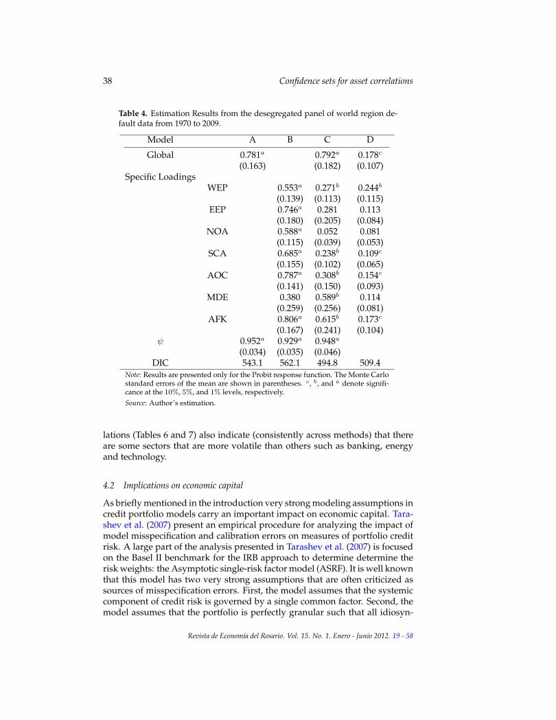
Different types of factor models (models A through D) are considered forthe panel data of sectors (3), regions (table 4) and structured products (table 5).The tables report the posterior means and the standard errors for the modelparameters using the Probit type response function.12 For the parameters ineach model, on average convergence of the Markov chains was reached after4,000 to 6,000 iterations.
In general, the parameters indicate that the global systemic factor loadingis statistically significant in all the models (Tables 3 to 5), except for model Din the sectors and regions. On the other hand, the local systemic factor weightis not always statistically significant. For example, the extreme case is modelD for regions, where the overall factors (except in the case of Western Europe)do not play a role in the dynamics of defaults.
Once convergence is obtained, the DIC indicates that the most appropriatemodel is model C for sectors and regions, and model D for products. Model Cis a two factor model that has an autoregressive global unobserved factor anda unique i.i.d. component for the local systemic factor. This previous specifi-cation is the same as model 4 of McNeil and Wendin (2007) and it is one of themodels used to derived the asset correlations (Table 6). Model D has the samestructure as the model estimated in Demey et al. (2004) and the asset correla-tions derived from it are presented in Table 7. There is a striking differencebetween the asset correlations derived from both models. Asset correlationsderived from model C are much higher than the ones derived from model D,particularly in the case for sectors and regions. While the asset correlationsof model D are within the range of the Basel II (2006) recommended values(0.12,0.24), even lower in some cases, model C proposes much higher values,with a possible range of 0.3 to 0.5. Another way to look at it is to determine theprobability that the estimated asset correlation is within the Basel II bounds,
11Accounting for tail risk would also require to change the distribution of the firm-idiosyncratic component, ei,t. This has an effect on the choice of link function. In order to avoidthis additional complication only the distribution of the unobserved factor is modified. It is im-portant to note that the change is enough to loose the tractability of the distribution of the assetvalue, Vi,t.
12There were no significant differences between the response functions, only the Probit resultsare presented, but the Logit results are available upon request.
Revista de Economıa del Rosario. Vol. 15. No. 1. Enero - Junio 2012. 19 - 58

36 Confidence sets for asset correlations
0.00 0.05 0.10 0.15 0.20 0.25 0.30 0.35 0.40 0.45 0.50 0.55
2
4
6
Median ρ= 0.1382
Basel Bounds, 33%
AR(1)
0.04 0.06 0.08 0.10 0.12 0.14 0.16 0.18 0.20
5
10
15
20
Median ρ= 0.0896
Basel Bounds, 8.3%
i.i.d.
(a) All ratings
0.0 0.1 0.2 0.3 0.4 0.5
1
2
3
4
Median ρ= 0.3657
IG i.i.d.
0.1 0.2 0.3 0.4 0.5
2
4
6
Median ρ= 0.4217
IG AR(1)
0.05 0.10 0.15 0.20 0.25
5
10
15
20
Median ρ= 0.0827
NIG i.i.d.
0.0 0.1 0.2 0.3 0.4 0.5
2
4
6
Median ρ= 0.1292
NIG AR(1)
(b) Investment & Non-Investment Grade
Figure 3. Estimated Bounds vs. the Basel II recommended bounds. Posteriordistribution of implied asset correlations from a one-factor model.Note: Implied asset correlation depends critically on model assumptions.Source: Author’s estimation.
P (0.12 ≤ ρ ≤ 0.24), using the posterior distribution. Whereas in model C theprobabilities is well below 7% for regions, and for sectors and products theyare zero, in model D these same probabilities are 11% for regions and sec-tors and 5% for products. These results indicate that the Basel recommendedbounds are overoptimistic with respect to uncertainty surrounding asset de-pendence. Furthermore, in most of the models considered in this Section, theBasel recommended bounds are located in the left tail of the posterior distri-
Revista de Economıa del Rosario. Vol. 15. No. 1. Enero - Junio 2012. 19 - 58

Castro 37
Table 3. Estimation Results from the desegregated panel of economic sectordefault data from 1970 to 2009.
Model A B C D
0.878a 0.845a 0.170c
(0.117) (0.147) (0.094)Specific Loadings
BAN 0.809a 0.467a 0.446a
(0.128) (0.118) (0.110)CAI 0.773a 0.071c 0.074
(0.0989) (0.041) (0.045)COI 0.723a 0.101b 0.178a
(0.104) (0.051) (0.060)EAE 0.765a 0.412a 0.128c
(0.126) (0.096) (0.077)FIR 0.577a 0.177c 0.087
(0.163) (0.100) (0.064)MED 0.463b 0.292c 0.120c
(0.181) (0.158) (0.070)RET 0.636a 0.106 0.082
(0.123) (0.069) (0.058)SOV 0.774a 0.108 0.203a
(0.152) (0.089) (0.060)TEC 0.908a 0.259a 0.225a
(0.075) (0.056) (0.068)TRA 0.517a 0.272b 0.095
(0.139) (0.108) (0.067)UTL 0.706a 0.236c 0.192b
(0.162) (0.136) (0.093)ψ 0.962a 0.950a 0.956a
(0.0223) (0.020) (0.036)DIC 1520.5 1522.1 1341.8 1360.9
Note: Results are presented only for the Probit response function. The Monte Carlostandard errors of the mean are shown in parentheses. c, b, and a denote signifi-cance at the 10%, 5%, and 1% levels, respectively.Source: Author’s estimation.
bution of asset correlation hence they seem to be consistent with a low levelof systemic risk (figure 4).
The differences in the implied asset correlations due to the dynamics ofthe unobserved factors do not seem to be only an empirical issue, but theoret-ical as well. It also makes intuitive sense because even though the factors arestationary, the fact that there is persistence (in some cases it is very strong),implies that any shocks in the short run will not dissipate from year to year.This also can explain the clustering phenomenon (across sectors and regions)of the number of defaults that is observed in the stylized facts. The asset corre-
Revista de Economıa del Rosario. Vol. 15. No. 1. Enero - Junio 2012. 19 - 58
38 Confidence sets for asset correlations
Table 4. Estimation Results from the desegregated panel of world region de-fault data from 1970 to 2009.
Model A B C D
Global 0.781a 0.792a 0.178c
(0.163) (0.182) (0.107)Specific Loadings
WEP 0.553a 0.271b 0.244b
(0.139) (0.113) (0.115)EEP 0.746a 0.281 0.113
(0.180) (0.205) (0.084)NOA 0.588a 0.052 0.081
(0.115) (0.039) (0.053)SCA 0.685a 0.238b 0.109c
(0.155) (0.102) (0.065)AOC 0.787a 0.308b 0.154c
(0.141) (0.150) (0.093)MDE 0.380 0.589b 0.114
(0.259) (0.256) (0.081)AFK 0.806a 0.615b 0.173c
(0.167) (0.241) (0.104)ψ 0.952a 0.929a 0.948a
(0.034) (0.035) (0.046)DIC 543.1 562.1 494.8 509.4
Note: Results are presented only for the Probit response function. The Monte Carlostandard errors of the mean are shown in parentheses. c, b, and a denote signifi-cance at the 10%, 5%, and 1% levels, respectively.Source: Author’s estimation.
lations (Tables 6 and 7) also indicate (consistently across methods) that thereare some sectors that are more volatile than others such as banking, energyand technology.
4.2 Implications on economic capital
As briefly mentioned in the introduction very strong modeling assumptions incredit portfolio models carry an important impact on economic capital. Tara-shev et al. (2007) present an empirical procedure for analyzing the impact ofmodel misspecification and calibration errors on measures of portfolio creditrisk. A large part of the analysis presented in Tarashev et al. (2007) is focusedon the Basel II benchmark for the IRB approach to determine determine therisk weights: the Asymptotic single-risk factor model (ASRF). It is well knownthat this model has two very strong assumptions that are often criticized assources of misspecification errors. First, the model assumes that the systemiccomponent of credit risk is governed by a single common factor. Second, themodel assumes that the portfolio is perfectly granular such that all idiosyn-
Revista de Economıa del Rosario. Vol. 15. No. 1. Enero - Junio 2012. 19 - 58
Castro 39
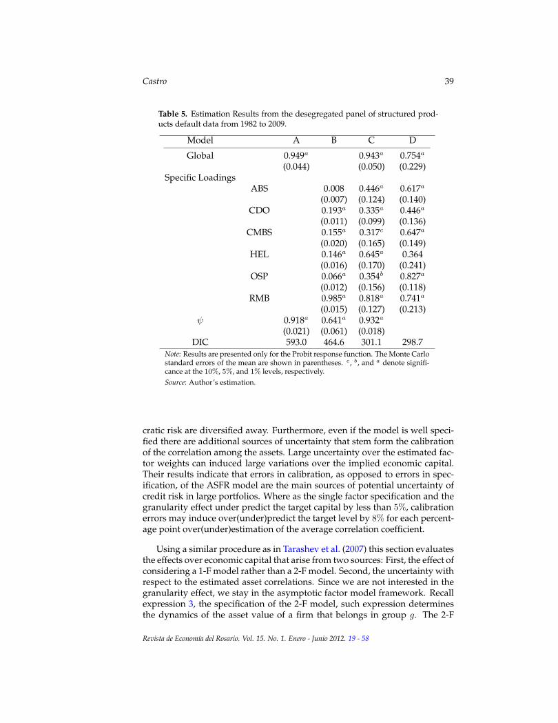
Table 5. Estimation Results from the desegregated panel of structured prod-ucts default data from 1982 to 2009.
Model A B C D
Global 0.949a 0.943a 0.754a
(0.044) (0.050) (0.229)Specific Loadings
ABS 0.008 0.446a 0.617a
(0.007) (0.124) (0.140)CDO 0.193a 0.335a 0.446a
(0.011) (0.099) (0.136)CMBS 0.155a 0.317c 0.647a
(0.020) (0.165) (0.149)HEL 0.146a 0.645a 0.364
(0.016) (0.170) (0.241)OSP 0.066a 0.354b 0.827a
(0.012) (0.156) (0.118)RMB 0.985a 0.818a 0.741a
(0.015) (0.127) (0.213)ψ 0.918a 0.641a 0.932a
(0.021) (0.061) (0.018)DIC 593.0 464.6 301.1 298.7
Note: Results are presented only for the Probit response function. The Monte Carlostandard errors of the mean are shown in parentheses. c, b, and a denote signifi-cance at the 10%, 5%, and 1% levels, respectively.Source: Author’s estimation.
cratic risk are diversified away. Furthermore, even if the model is well speci-fied there are additional sources of uncertainty that stem form the calibrationof the correlation among the assets. Large uncertainty over the estimated fac-tor weights can induced large variations over the implied economic capital.Their results indicate that errors in calibration, as opposed to errors in spec-ification, of the ASFR model are the main sources of potential uncertainty ofcredit risk in large portfolios. Where as the single factor specification and thegranularity effect under predict the target capital by less than 5%, calibrationerrors may induce over(under)predict the target level by 8% for each percent-age point over(under)estimation of the average correlation coefficient.
Using a similar procedure as in Tarashev et al. (2007) this section evaluatesthe effects over economic capital that arise from two sources: First, the effect ofconsidering a 1-F model rather than a 2-F model. Second, the uncertainty withrespect to the estimated asset correlations. Since we are not interested in thegranularity effect, we stay in the asymptotic factor model framework. Recallexpression 3, the specification of the 2-F model, such expression determinesthe dynamics of the asset value of a firm that belongs in group g. The 2-F
Revista de Economıa del Rosario. Vol. 15. No. 1. Enero - Junio 2012. 19 - 58

40 Confidence sets for asset correlations
Table 6. Asset correlations obtained from the default risk model. Model typeC and Probit response function.
Model C 2.5 Mean 97.5
Global 0.150 0.329 0.396
Banking 0.283 0.482 0.583Capital industries 0.182 0.415 0.500Consumer Industies 0.187 0.417 0.501Energy & Environment 0.267 0.469 0.560Finance, Insurance & Real Estate 0.198 0.427 0.516Media & Publishing 0.230 0.447 0.555Retail & Distribution 0.189 0.418 0.503Sovereign & Public Finance 0.188 0.419 0.506Technology 0.215 0.436 0.520Transportation 0.221 0.441 0.534Utilities 0.206 0.437 0.538
Global 0.088 0.301 0.392
Western Europe 0.154 0.412 0.534Eastern Europe 0.139 0.420 0.582North America 0.105 0.383 0.498Central & South America 0.148 0.406 0.521Asia & Oceania 0.153 0.421 0.553Middle East 0.227 0.499 0.642Africa 0.241 0.506 0.643
Global 0.310 0.367 0.391
ABS 0.442 0.523 0.593CDO 0.442 0.502 0.552CMBS 0.430 0.502 0.577HEL 0.476 0.567 0.651OSP 0.415 0.507 0.591RMB 0.514 0.608 0.660Source: Author’s estimation.
model can be expressed such that it nest the 1-F model:
Vi,t :=√ρBt +
√∆ρgBg,t +
√1− (ρ+∆ρg)ei,t,∀i ∈ g, (7)
where ∆ρg = ρg − ρ measures the difference between inter and intra correla-tion. By definition ∆ρg ≥ 0. This implies that there is some diversification af-fect by holding positions in different groups (sectors or world regions) ratherthan concentrating all exposures in a particular group. The limit of the diver-
Revista de Economıa del Rosario. Vol. 15. No. 1. Enero - Junio 2012. 19 - 58

Castro 41
Table 7. Asset correlations obtained from the default risk model. Model typeD and Probit response function.
Model D 2.5 Mean 97.5
Global 0.000 0.032 0.093
Banking 0.080 0.193 0.348Capital industries 0.002 0.042 0.111Consumer Industies 0.013 0.066 0.146Energy & Environment 0.003 0.055 0.138Finance, Insurance & Real Estate 0.002 0.046 0.123Media & Publishing 0.003 0.053 0.134Retail & Distribution 0.002 0.045 0.119Sovereign & Public Finance 0.018 0.075 0.153Technology 0.022 0.083 0.174Transportation 0.003 0.047 0.124Utilities 0.032 0.076 0.146
Global 0.000 0.036 0.112
Western Europe 0.010 0.099 0.233Eastern Europe 0.002 0.057 0.153North America 0.001 0.048 0.133Central & South America 0.002 0.054 0.142Asia & Oceania 0.004 0.068 0.157Middle East 0.002 0.057 0.150Africa 0.010 0.076 0.158
Global 0.025 0.277 0.386
ABS 0.229 0.489 0.624CDO 0.143 0.437 0.572CMBS 0.276 0.501 0.620HEL 0.056 0.416 0.615OSP 0.341 0.556 0.655RMB 0.299 0.538 0.642Source: Author’s estimation.
sification effect is determined by the global systemic risk (non-diversifiablerisk). If ∆ρg = 0 then we obtain the 1-F model and this means that thereare no further gains obtained by holding positions across different groups offirms.
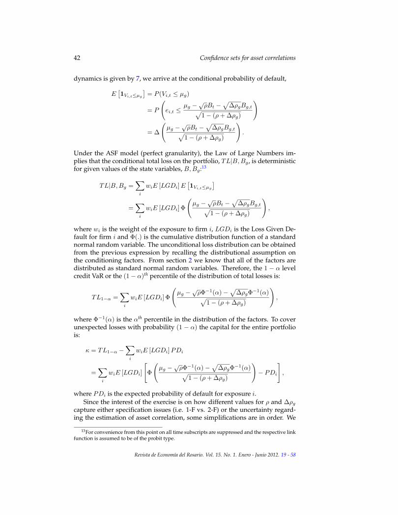
Following Tarashev et al. (2007), let 1Vi,t≤µg denote an indicator variablethat is equal to 1 if firm i ∈ g is in default at time t and, 0 otherwise. By takingexpectations over the indicator variable and assuming that the asset value
Revista de Economıa del Rosario. Vol. 15. No. 1. Enero - Junio 2012. 19 - 58
42 Confidence sets for asset correlations
dynamics is given by 7, we arrive at the conditional probability of default,
E[1Vi,t≤µg
]= P (Vi,t ≤ µg)
= P
(ei,t ≤
µg −√ρBt −
√∆ρgBg,t√
1− (ρ+∆ρg)
)
= ∆
(µg −
√ρBt −
√∆ρgBg,t√
1− (ρ+∆ρg)
).
Under the ASF model (perfect granularity), the Law of Large Numbers im-plies that the conditional total loss on the portfolio, TL|B,Bg , is deterministicfor given values of the state variables, B,Bg :13
TL|B,Bg =∑i
wiE [LGDi]E[1Vi,t≤µg
]=∑i
wiE [LGDi] Φ
(µg −
√ρBt −
√∆ρgBg,t√
1− (ρ+∆ρg)
),
where wi is the weight of the exposure to firm i, LGDi is the Loss Given De-fault for firm i and Φ(.) is the cumulative distribution function of a standardnormal random variable. The unconditional loss distribution can be obtainedfrom the previous expression by recalling the distributional assumption onthe conditioning factors. From section 2 we know that all of the factors aredistributed as standard normal random variables. Therefore, the 1 − α levelcredit VaR or the (1− α)th percentile of the distribution of total losses is:
TL1−α =∑i
wiE [LGDi] Φ
(µg −
√ρΦ−1(α)−
√∆ρgΦ
−1(α)√1− (ρ+∆ρg)
),
where Φ−1(α) is the αth percentile in the distribution of the factors. To coverunexpected losses with probability (1 − α) the capital for the entire portfoliois:
κ = TL1−α −∑i
wiE [LGDi]PDi
=∑i
wiE [LGDi]
[Φ
(µg −
√ρΦ−1(α)−
√∆ρgΦ
−1(α)√1− (ρ+∆ρg)
)− PDi
],
where PDi is the expected probability of default for exposure i.Since the interest of the exercise is on how different values for ρ and ∆ρg
capture either specification issues (i.e. 1-F vs. 2-F) or the uncertainty regard-ing the estimation of asset correlation, some simplifications are in order. We
13For convenience from this point on all time subscripts are suppressed and the respective linkfunction is assumed to be of the probit type.
Revista de Economıa del Rosario. Vol. 15. No. 1. Enero - Junio 2012. 19 - 58
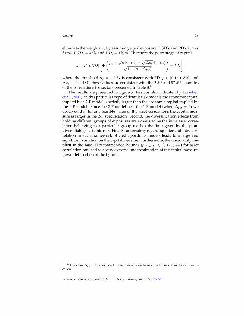
Castro 43
eliminate the weights wi by assuming equal exposure, LGD’s and PD’s acrossfirms, LGDi = 45% and PDi = 1% ∀i. Therefore the percentage of capital,
κ = E [LGD]
[Φ
(µg −
√ρΦ−1(α)−
√∆ρgΦ
−1(α)√1− (ρ+∆ρg)
)− PD
],
where the threshold µg = −2.37 is consistent with PD. ρ ∈ [0.15, 0.396] and∆ρg ∈ [0, 0.187], these values are consistent with the 2.5th and 97.5th quantilesof the correlations for sectors presented in table 8.14
The results are presented in figure 5. First, as also indicated by Tarashevet al. (2007), in this particular type of default risk models the economic capitalimplied by a 2-F model is strictly larger than the economic capital implied bythe 1-F model. Since the 2-F model nest the 1-F model (when ∆ρg = 0) weobserved that for any feasible value of the asset correlations the capital mea-sure is larger in the 2-F specification. Second, the diversification effects fromholding different groups of exposures are exhausted as the intra asset corre-lation belonging to a particular group reaches the limit given by the (non-diversifiable) systemic risk. Finally, uncertainty regarding inter and intra cor-relation in such framework of credit portfolio models leads to a large andsignificant variation on the capital measure. Furthermore, the uncertainty im-plicit in the Basel II recommended bounds (ρBaselII ∈ [0.12, 0.24]) for assetcorrelation can lead to a very extreme underestimation of the capital measure(lower left section of the figure).
14The value ∆ρg = 0 is included in the interval so as to nest the 1-F model in the 2-F specifi-cation.
Revista de Economıa del Rosario. Vol. 15. No. 1. Enero - Junio 2012. 19 - 58

44 Confidence sets for asset correlations
0.0 0.2 0.4
5
10Global
0.25 0.50
2.5
5.0
7.5 BAN
0.0 0.2 0.4
2.5
5.0
7.5
10.0CAI
0.0 0.2 0.4 0.6
2.5
5.0
7.5
10.0COI
0.25 0.50
2.5
5.0
7.5
10.0EAE
0.00 0.25 0.50
2.5
5.0
7.5
10.0FIR
0.00 0.25 0.50
2.5
5.0
7.5 MED
0.00 0.25 0.50
2.5
5.0
7.5
10.0RET
0.00 0.25 0.50
2.5
5.0
7.5
10.0SOV
0.00 0.25 0.50
2.5
5.0
7.5
10.0TEC
0.00 0.25 0.50
2.5
5.0
7.5
10.0TRA
0.00 0.25 0.50
2.5
5.0
7.5 UTL
(a) Economic Sectors
0.0 0.1 0.2 0.3 0.4
2.5
5.0
7.5 Global
0.1 0.2 0.3 0.4 0.5 0.6
2.5
5.0
7.5WEP
0.0 0.1 0.2 0.3 0.4 0.5 0.6 0.7
2.5
5.0EEP
0.0 0.1 0.2 0.3 0.4 0.5
2.5
5.0
7.5NOA
0.0 0.1 0.2 0.3 0.4 0.5 0.6
2.5
5.0
7.5SCA
0.1 0.2 0.3 0.4 0.5 0.6 0.7
2.5
5.0AOC
0.0 0.1 0.2 0.3 0.4 0.5 0.6 0.7
2
4MDE
0.0 0.1 0.2 0.3 0.4 0.5 0.6 0.7
2
4AFK
(b) World Regions
0.275 0.300 0.325 0.350 0.375 0.400
10
20
30Global
0.40 0.45 0.50 0.55 0.60 0.65
5
10
15ABS
0.40 0.45 0.50 0.55 0.60
5
10
15 CDO
0.40 0.45 0.50 0.55 0.60 0.65
5
10
15 CMBS
0.40 0.45 0.50 0.55 0.60 0.65
2.5
5.0
7.5 HEL
0.40 0.45 0.50 0.55 0.60 0.65
5
10
15OSP
0.45 0.50 0.55 0.60 0.65
5
10RMB
(c) Structured Products
Figure 4. Posteriors distributions for implied asset correlations (Model C).Source: Author’s estimation.
Revista de Economıa del Rosario. Vol. 15. No. 1. Enero - Junio 2012. 19 - 58

Castro 45
Figure 5. Implications on economic capital of the uncertainty over the esti-mate of asset correlations in a dynamic factor model of default risk.Source: Author’s compilation.
Revista de Economıa del Rosario. Vol. 15. No. 1. Enero - Junio 2012. 19 - 58
46 Confidence sets for asset correlations
5 Attenuating over-dispersion in the data with a zero-inflated binomialmodel
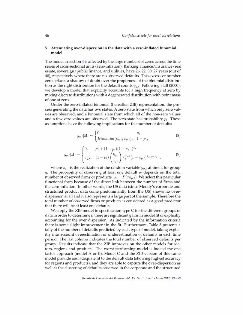
The model in section 4 is affected by the large numbers of zeros across the timeseries of cross sectional units (zero-inflation). Banking, finance/insurance/realestate, sovereign/public finance, and utilities, have 26, 22, 30, 27 years (out of40), respectively where there are no observed defaults. This excessive numberzeros places a shadow of doubt over the properness of the binomial distribu-tion as the right distribution for the default counts yg,t. Following Hall (2000),we develop a model that explicitly accounts for a high frequency at zero bymixing discrete distributions with a degenerated distribution with point massof one at zero.
Under the zero-inflated binomial (hereafter, ZIB) representation, the pro-cess generating the data has two states. A zero state from which only zero val-ues are observed, and a binomial state from which all of the non-zero valuesand a few zero values are observed. The zero state has probability pt. Theseassumptions have the following implications for the number of defaults:
yg,t|Bt ∼
0, pt
Binomial(kg,t, πg,t), 1− pt,(8)
yg,t|Bt =
0, pt + (1− pt)(1− πg,t)
kg,t
zg,t, (1− pt)
(kg,t
zg,t
)πzg,tt (1− πg,t)
kg,t−zg,t ,(9)
where zg,t is the realization of the random variable yg,t at time t for groupg. The probability of observing at least one default pt depends on the totalnumber of observed firms or products, pt = P (τkg,t). We select this particularfunctional form because of the direct link between the number of firms andthe zero-inflation. In other words, the US data (since Moody’s corporate andstructured product data come predominantly from the US) shows no over-dispersion at all and it also represents a large part of the sample. Therefore thetotal number of observed firms or products is considered as a good predictorthat there will be at least one default.
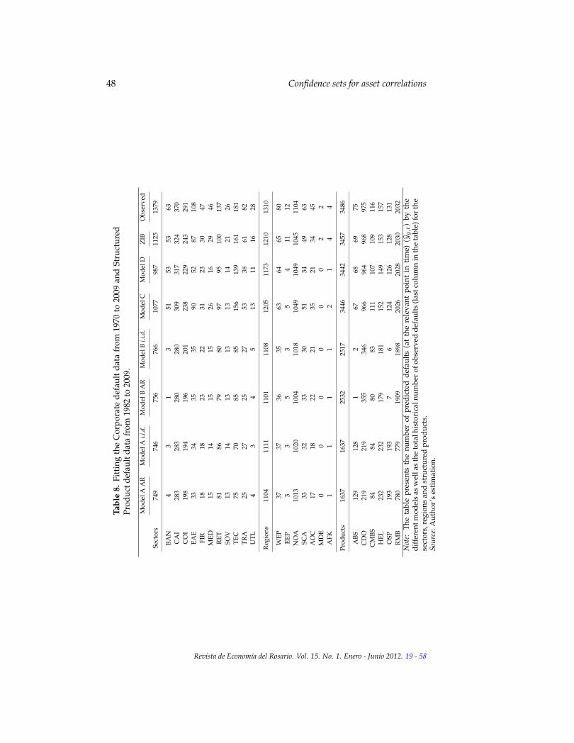
We apply the ZIB model to specification type C for the different groups ofdata in order to determine if there are significant gains in model fit of explicitlyaccounting for the over dispersion. As indicated by the information criteriathere is some slight improvement in the fit. Furthermore, Table 8 presents atally of the number of defaults predicted by each type of model, taking explic-itly into account overestimation or underestimation of defaults in each timeperiod. The last column indicates the total number of observed defaults pergroup. Results indicate that the ZIB improves on the other models for sec-tors, regions and products. The worst performing model is indeed the onefactor approach (model A or B). Model C and the ZIB version of this samemodel provide and adequate fit to the default data (showing highest accuracyfor regions and products), and they are able to capture the over-dispersion aswell as the clustering of defaults observed in the corporate and the structured
Revista de Economıa del Rosario. Vol. 15. No. 1. Enero - Junio 2012. 19 - 58

Castro 47
product data. Asset correlations derived from the ZIB model are presented inTable 9, they are slightly higher for sectors and regions and lower for prod-ucts than those of model C (Table 6) but, the variation within each group ismaintained. For example, as was observed in Section 4, the more volatile sec-tors and products are banking, energy, technology, and residential mortgagebacked securities, respectively.
Revista de Economıa del Rosario. Vol. 15. No. 1. Enero - Junio 2012. 19 - 58
48 Confidence sets for asset correlations
Tabl
e8.
Fitt
ing
the
Cor
pora
tede
faul
tdat
afr
om19
70to
2009
and
Stru
ctur
edPr
oduc
tdef
ault
data
from
1982
to20
09.
Mod
elA
AR
Mod
elA
i.i.d
.M
odel
BA
RM
odel
Bi.i
.d.
Mod
elC
Mod
elD
ZIB
Obs
erve
d
Sect
ors
749
746
756
766
1077
987
1125
1379
BAN
43
13
5153
5363
CA
I28
328
328
028
030
931
732
437
0C
OI
198
194
196
201
238
229
243
291
EAE
3334
3535
9052
8710
8FI
R18
1823
2231
2330
47M
ED15
1415
1526
1629
46R
ET81
8679
8097
9510
013
7SO
V13
1413
1313
1421
26TE
C75
7085
8515
613
916
118
1TR
A25
2725
2753
3861
82U
TL4
34
513
1116
28
Reg
ions
1104
1111
1101
1108
1205
1173
1210
1310
WEP
3737
3635
6364
6580
EEP
33
53
54
1112
NO
A10
1310
2010
0410
1810
4910
4910
4511
04SC
A33
3233
3051
3449
63A
OC
1718
2221
3521
3445
MD
E0
00
00
02
2A
FK1
11
12
14
4
Prod
ucts
1637
1637
2532
2517
3446
3442
3457
3486
ABS
129
128
12
6768
6975
CD
O21
921
935
534
696
696
496
897
5C
MBS
8484
8083
111
107
109
116
HEL
232
232
179
181
152
149
153
157
OSP
193
193
76
124
126
128
131
RM
B78
077
919
0918
9820
2620
2820
3020
32N
ote:
The
tabl
epr
esen
tsth
enu
mbe
rof
pred
icte
dde
faul
ts(a
tth
ere
leva
ntpo
int
inti
me)
(yg,t)
byth
edi
ffer
entm
odel
sas
wel
las
the
tota
lhis
tori
caln
umbe
rof
obse
rved
defa
ults
(las
tcol
umn
inth
eta
ble)
for
the
sect
ors,
regi
ons
and
stru
ctur
edpr
oduc
ts.
Sour
ce:A
utho
r’s
esti
mat
ion.
Revista de Economıa del Rosario. Vol. 15. No. 1. Enero - Junio 2012. 19 - 58

Castro 49
Table 9. Asset correlations obtained from the default risk model. Zero-Inflated model (ZIB) of type C and Probit response function.
Model ZIB 2.5 Mean 97.5
Global 0.147 0.322 0.396
Banking 0.241 0.441 0.540Capital industries 0.184 0.409 0.503Consumer Industies 0.182 0.406 0.501Energy & Environment 0.216 0.425 0.519Finance, Insurance & Real Estate 0.184 0.409 0.506Media & Publishing 0.182 0.411 0.510Retail & Distribution 0.178 0.404 0.499Sovereign & Public Finance 0.179 0.406 0.500Technology 0.216 0.426 0.517Transportation 0.176 0.404 0.500Utilities 0.179 0.406 0.501
Global 0.065 0.242 0.391
Western Europe 0.088 0.312 0.500Eastern Europe 0.093 0.328 0.525North America 0.080 0.303 0.495Central & South America 0.096 0.319 0.504Asia & Oceania 0.096 0.323 0.508Middle East 0.139 0.416 0.622Africa 0.135 0.414 0.621
Global 0.280 0.347 0.390
ABS 0.405 0.499 0.597CDO 0.397 0.481 0.556CMBS 0.382 0.475 0.576HEL 0.398 0.496 0.609OSP 0.393 0.483 0.570RMB 0.480 0.553 0.646Note: The table presents the number of predicted defaults (at the relevantpoint in time) (yg,t) by the different models as well as the total historicalnumber of observed defaults (last column in the table) for the sectors,regions and structured products.Source: Author’s estimation.
Revista de Economıa del Rosario. Vol. 15. No. 1. Enero - Junio 2012. 19 - 58
50 Confidence sets for asset correlations
6 Conclusions
An important change form the Basel I to the Basel II accord, with respect thetechnicalities associated to the estimation of capital requirements, addressesthe issue of accounting for as much of the heterogeneity as possible in the de-termination of the risk weights associated with each position in a portfolio.This has been a topic of ongoing research. However, there are some issuesso far unresolved: First, the professional tools that are available concentrateon equity data to measure dependence (correlation) across groups of issuers(industries, countries); even thought changes in equity data may not be anadequate proxy of the changes in credit quality. A good example of thesemethodologies is CreditMetrics and Moody’s KMV.15 Second, when ratingdata has been used to characterize dependence the authors (with some ex-ceptions) have dealt with the problem of estimating the parameters of intereston aggregated data. In part this is due to the difficulties of working with therating data where the rare events (defaults in particular) are the most interest-ing but making inference on them is complex.
This paper complements research on asset correlation estimates across sec-tors using rating data and presents some new results on regions and struc-tured products.16. We use the methodology developed by Wendin (2006);Wendin and McNeil (2006) and McNeil and Wendin (2007), along with pub-licly available software WINBUGS. With the aggregate data and in the onefactor framework, results are very similar to the ones obtained by the previ-ous authors.
With Bayesian methods, we offer results for a large number of disaggre-gated units (11 sectors, 7 world regions and 6 structured products). Bayesianmethods make it possible to obtain estimates even with over dispersion ofthe data (Zero-Inflation), they also allow for a straightforward set up of ad-ditional mixtures in order to properly account for the zeros through a Zero-Inflated Binomiam model (ZIP). This ZIP provides in some cases substantialimprovement in fitting the time series of defaults.
The loading parameters of the factors across the sectors, regions and struc-tured products models are in general statistically significant. From these fac-tor weights it is possible to recover the asset correlations. Asset correlationsare in most cases higher than the Basel II recommended values. They arealso higher if the unobserved component is autoregressive as opposed to i.i.d.The two factor model with AR(1) dynamics for global factor and with a localsystemic factor is able to reproduce better the observed number of defaultsthan the one factor framework recommended by Basel II. In the panels, theUS data determines most of the global factor dynamics. This is expected sincethe database is predominately composed of US firms.
Overall this chapter presents a set of asset correlation estimates for eco-nomic sectors, world regions and structured products that can be used forcredit portfolio modeling. It also indicates some caution in the use of the Basel
15See Gupton et al. (1997) and Crosbie (2005).16See Gordy and Heitfield (2002); Demey et al. (2004); Servigny and Renault (2003); Wendin
and McNeil (2006); McNeil and Wendin (2007)
Revista de Economıa del Rosario. Vol. 15. No. 1. Enero - Junio 2012. 19 - 58

Castro 51
recommended bounds for asset correlation in portfolio risk models. First,these bounds in general tend to be over optimistic with respect to the de-pendence structure that is consistent with the historical default data (figures3 to 5). Second, with some certainty these bounds do not hold equally forall exposures (there are differences observed in the estimates of asset correla-tions between sectors, regions and structured products. Third, the modelingassumptions used in the estimation of these implied asset correlations carrysubstantial model risk to the measurement of economic capital. Therefore, atransparent and proper sensibility analysis to the assumptions that give riseto the dependence structure should be an integral part of the portfolio creditrisk model validation process.
Revista de Economıa del Rosario. Vol. 15. No. 1. Enero - Junio 2012. 19 - 58
52 Confidence sets for asset correlations
Appendix
A.1 Derivation of the full conditional distributions for Bayesian estimation.
We obtain Bayesian estimates of the parameters of interest through the use ofa Markov Chain Monte Carlo algorithm such as the Gibbs sampler. Imple-mentation of the Gibbs sampler requires the derivation of the full conditionaldistributions of the elements of the models. This set of full conditional distri-butions are sampled in a way so as to derive the joint posterior distributions ofthe parameters of interest. Borrowing notation from Gilks et al. (1996) and Mc-Neil and Wendin (2007), [X] denotes the (unconditional) density of X, [X|Y ]the conditional density of X given Y and [X|.] the full conditional of X.
We derive in the following subsections the full conditional distributionsfor model A (univariate model), C (multivariate model) and the zero-inflatedbinomial model.
A.2 Model A (univariate one factor model)
In the univariate case X := (X1, ..., XT ). First recall the main elements of thisstate space model: The measurement equation,
yt|Bt ∼ Binomial(kt,Φ
(µ−
√ρ
√1− ρ
Bt
)), t = 1, .., T,
the state equation,Bt = ψBt−1+√1− ψ2ηt, ηt ∼ N(0, 1). With prior distribu-
tions for the unknown parameters ψ ∼ U(−1, 1), ϱ(ρ) :=√ρ√
1−ρ ∼ U(0, 10) andµ ∼ N(0, σ2
µ = 103). Note that the unobserved component has a multivariateGaussian distribution, B ∼ N(0,Ω).
Ω =1
1− ψ2
1 ψ . . . ψT−1
ψ 1. . . ψT−2
......
. . ....
ψT−1 ψT−2 . . . 1
.
The multivariate Gaussian density of B is
fB(ψ) = (2π)−T/2 | Ω−1 |1/2 exp[−1
2
(B′Ω−1B
)].
A first step in deriving the full conditional distribution is to write out the jointdistribution function of the data and the unknowns (parameters and unob-served components). This joint distribution can be further simplified giventhe conditional independence and unconditional independence across someof it elements. For example, assumptions on the model determine that de-faults (yt) are independent across time conditional on the unobserved compo-nent Bt. Furthermore, the parameters of interest (ψ, ϱ(ρ), µ), are themselves
Revista de Economıa del Rosario. Vol. 15. No. 1. Enero - Junio 2012. 19 - 58

Castro 53
independent
[y, k,B, µ, ϱ(ρ), ψ] = [y | k,B, µ, ϱ(ρ)][B | ψ][µ][ϱ(ρ)][ψ],
=
(T∏t=1
[yt | kt, Bt, µ, ϱ(ρ)][Bt | ψ]
)[µ][ϱ(ρ)][ψ],
this expression represents a form of fragmentation of the joint distribution ofthe data and the unknowns. In particular there are five relevant fragments(conditional and unconditional distributions). The final step of deriving thefull conditional distribution of any of the parameters of interest is to apply theconditional probability formula and pick out only the fragments that dependexplicitly on the parameter of interest. The sign ∝ denotes a form of equiva-lence (proportional to), during the process of selecting the relevant fragments.
The full conditional for ψ is:
[ψ | .] =[y, k,B, µ, ϱ(ρ), ψ]
[y, k,B, µ, ϱ(ρ)]∝ [y, k,B, µ, ϱ(ρ)] ∝ [B | ψ][ψ],
∝ | Ω−1 |1/2 exp[−1
2
(B′Ω−1B
)] 121(−1≤ψ≤1).
An expression for the conditional distribution of defaults is required forall of the other full conditional distributions:
T∏t=1
[yt | kt, Bt, µ, ϱ(ρ)] ∝T∏t=1
Φ(µ− ϱ(ρ)Bt)yt [1− Φ(µ− ϱ(ρ)Bt)]
kt−yt .
The full conditional for ϱ(ρ) is:
[ϱ(ρ) | .] =[y, k,B, µ, ϱ(ρ), ψ]
[y, k,B, µ, ψ]∝ [y, k,B, µ, ϱ(ρ), ψ]
∝T∏t=1
[yt | kt, Bt, µ, ϱ(ρ)][ϱ(ρ)],
∝T∏t=1
Φ (µ− ϱ(ρ)Bt)yt [1− Φ (µ− ϱ(ρ)Bt)]
kt−yt 1
101(0≤ϱ(ρ)≤10).
The full conditional for µ is:
[µ | .] =[y, k,B, µ, ϱ(ρ), ψ]
[y, k,B, ϱ(ρ), ψ]∝ [y, k,B, µ, ϱ(ρ), ψ]
∝T∏t=1
[yt | kt, Bt, µ, ϱ(ρ)][µ],
∝T∏t=1
Φ(µ− ϱ(ρ)Bt)yt [1− Φ(µ− ϱ(ρ)Bt)]
kt−yt(2πσ2µ)
−1/2
exp
(−1
2
µ2
σ2µ
).
Revista de Economıa del Rosario. Vol. 15. No. 1. Enero - Junio 2012. 19 - 58

54 Confidence sets for asset correlations
Since the unobserved component Bt is a T dimensional process then eachcomponent must be treated individually. It is also important to take intoaccount that since Bt is AR(1) then the realization of such process dependson its immediate neighbors. Denote the vector B without the t element asB−t := (B1, . . . , Bt−1, Bt+1.., BT ). Under these assumptions the full condi-tional for Bt is:
[Bt | .] =[y, k,B, µ, ϱ(ρ), ψ]
[y, k, ϱ(ρ), ψ]∝ [y, k,B, µ, ϱ(ρ), ψ],
∝T∏t=1
[yt | kt, Bt, µ, ϱ(ρ)][Bt | Bt−1, Bt+1, ψ].
An smooth estimate (two-sided filter) is obtained for the conditional dis-tribution ofBt givenB−t, with a forward and backward looking element (onesided filter) at the origin and at the end, respectively,
[B1 | B1, B2, ψ] =
(2π
1
1− ψ2
)−1/2
exp
(−1
2
(B2 − ψB1)2
11−ψ2
),
[Bt | Bt−1, Bt+1, ψ] =
(2π
1
1− ψ2
)−1/2
exp
(−1
2
(Bt − ψ2 (Bt−1 +Bt+1))
2
11−ψ2
),
[BT | BT−1, BT , ψ] =
(2π
1
1− ψ2
)−1/2
exp
(−1
2
(BT − ψBT−1)2
11−ψ2
).
Because of the structure of the state-space model, it is not possible to re-duced analytically the full conditional likelihood derived previously in orderto get a closed-form distribution. The current setup requires the use of effi-cient algorithms (such as adaptive rejection sampling or Metropolis-Hastings)to sample the distributions, Gilks et al. (1996).
A.3 Model C (multivariate two factor model)
In the multivariate case X := (X1,1, ..., XT,G). First recall the main elementsof this state space model: The measurement equation,
yg,t|Bt ∼ Binomial(kg,t,Φ(µg − ϱ(ρ)Bt − ϱ(ρ)gBt,g)), g = 1, .., G; t = 1, .., T,
the state equation, Bt = ΦBt−1 + Θηt, ηt ∼ N(0, I). Φ = diag(ψ,ψ1, ..., ψG),Θ = diag(
√1− ψ2,
√1− ψ2
1 , ...,√1− ψ2
G). With prior distributions for the
unknown parameters ψ,ψg ∼ U(−1, 1), ϱ(ρ) :=√ρ√
1−ρg,ϱg(ρ) :=
√ρg−ρ√1−ρg
∼
U(0, 10) and µg ∼ N(0, σ2µ = 103), g = 1, ...G. Note that the unobserved com-
ponent has a multivariate Gaussian distribution, Bt ∼ N(ΦBt−1,Ω). Then themultivariate Gaussian density of B is
fBt|Bt−1(Φ) = (2π)−(G+1)/2 | Ω−1 |1/2 exp
[((Bt − ΦBt−1)
′Ω−1(Bt − ΦBt−1))].
Revista de Economıa del Rosario. Vol. 15. No. 1. Enero - Junio 2012. 19 - 58

Castro 55
The fragmentation of the joint distribution of the data and the unknowns,under this model, is:
[y, k,B, µ, ϱ(ρ), ψ] = [y | k,B, µ, ϱ(ρ)][B | ψ][µ][ϱ(ρ)][ψ],
=
(T∏t=1
G∏g=1
[yg,t | kg,t,Bt, µ, ϱ(ρ)][Bt | ψ]
)[µ][ϱ(ρ)][ψ],
where µ := (µ1, ..., µG),ϱ(ρ) := (ϱ(ρ), ϱ(ρ)1, ..., ϱ(ρ)G), ψ := (ψ,ψ1, ..., ψG).The full conditional distributions of the elements in the multivariate modelsare found analogously, using the procedures presented for the univariate case.
A.4 Zero-Inflated Binomial model
In the multivariate case X := (X1,1, ..., XT,G). First recall the main elementsof this state space model that incorporates an additional mixture in order todistinguish the two relevant states yg,t = 0 (no defaults) or yg,t = 0 (in whichcase the number of defaults is denoted as zg,t): The measurement equationcapture these two states,
yg,t|Bt =
0, pg,t + (1− pt)(1− πg,t)
kg,t ,
zg,t, (1− pg,t)
(kg,t
zg,t
)πzg,tt (1− πg,t)
kg,t−zg,t ,
the state equation, Bt = ΦBt−1 +Θηt, ηt ∼ N(0, I). The priors for (µ, ψ, ϱ(ρ))have the same characteristics of the previous model. An additional signal isintroduced pg,t = P (τkg,t), with the following prior for τ ∼ N(0, σ2
τ = 103).The easiest form of presenting the ZIB model is to segment the observed
defaults y := (y0, z), where z denotes the non-zero values of y, which is astacked vector of of dimensions ((TxG)x1). Let y be arranged such that thefirst m elements are in y0 (zero defaults) and elements from m + 1 to L are inz (non-zero defaults).
The fragmentation of the joint distribution of the data and the unknowns,under this model, is:
[y, k,B, p, µ, ϱ(ρ), ψ, τ ] = [y | k,B, p, µ, ϱ(ρ)][B | ψ][p | k, τ ][µ][ϱ(ρ)][ψ][τ ]
An expression for the conditional distribution of defaults is required forall of the other full conditional distributions. For observations 1...m:
m∏l=1
G∏g=1
[y0g,l | kg,l,Bl, pg,l, µ, ϱ(ρ), τ ] ∝,
m∏l=1
G∏g=1
P (τkg,l) + (1− P (τkg,l))[1− Φ(µg − ϱ(ρ)Bl − ϱ(ρ)gBl,g)]kg,l ,
Revista de Economıa del Rosario. Vol. 15. No. 1. Enero - Junio 2012. 19 - 58

56 Confidence sets for asset correlations
for observations m+ 1...L:
L∏l=m+1
G∏g=1
[zg,l | kg,l,Bl, pg,l, µ, ϱ(ρ), τ ] ∝,
L∏l=m+1
G∏g=1
(1− P (τkg,l))Φ (µg − ϱ(ρ)Bl − ϱ(ρ)gBl,g)zg,l ,
[1− Φ(µg − ϱ(ρ)Bl − ϱ(ρ)gBl,g)]kg,l−zg,l .
The full conditional distributions of the elements in the ZIB model arefound analogously, using the procedures presented for the univariate case.
Revista de Economıa del Rosario. Vol. 15. No. 1. Enero - Junio 2012. 19 - 58

Castro 57
References
Akhavein, J., A. Kocaqil, and M. Neugebauer (2005). A comparative empiricalstudy of asset correlations. Report, Fitch Ratings.
Bangia, A., F. X. Diebold, A. Kronimus, C. Schagen, and T. Schuermann (2002).Ratings migration and the business cycle, with application to credit portfo-lio stress testing. Journal of Banking & Finance 26(2-3), 445–474.
Chernih, A., S. Vanduffel, and L. Henrard (2006). Asset correlations: a liter-ature review and analysis of the impact of dependent loss given defaults.Working paper.
Crosbie, P. (2005). Global correlation factor structure, modeling methodology.Technical report, Moody’s KMV company.
Das, S., D. Duffie, N. Kapadia, and L. Saita (2007). Common failings: Howcorporate defaults are correlated. Journal of Finance 62(1), 93–117.
Das, S. and G. Gengb (2004). Correlated default processes: a criterion-basedcopula approach. Journal of investment management 2(2), 44–70.
Demey, P., J. Jouanin, C. Roget, and T. Roncalli (2004). Maximum likelihoodestimate of default correlations. Risk.
Durbin, J. and J. Koopman (1997). Monte carlo maximum likelihood estima-tion for non-gaussian state space models. Biometrika 84(3), 669–684.
Gelman, A. and D. Rubin (1996). Markov chain monte carlo methods in bio-statistics. Statistical Methods in Medical Research 5(4), 339–355.
Gelman, A. and D. B. Rubin (1992). Inference from Iterative Simulation UsingMultiple Sequences. Statist.Sci. 7, 457–472.
Gilks, W., S. Richardson, and D. Spiegelhalter (1996). Markov chain monte carloin practice. Chapman and Hall CRC.
Gordy, M. and E. Heitfield (2002). Estimating default correlations from shortpanels of credit performance data. Technical report, Federal Reserve Board.
Gupton, G., C. Finger, and M. Bhatia (1997). Creditmetrics. Technical report,J.P. Morgan.
Kavvathas, D. (2001). Estimating credit rating transition probabilities for cor-porate bonds.
Koopman, S. and A. Lucas (2008). A non-gaussian panel time series model forestimating and decomposing default risk. Journal of Business and EconomicStatistics 26(4), 510–525.
Koopman, S. J., R. Kraussl, A. Lucas, and A. B. Monteiro (2009). Credit cyclesand macro fundamentals. Journal of Empirical Finance 16(1), 42–54.
Revista de Economıa del Rosario. Vol. 15. No. 1. Enero - Junio 2012. 19 - 58

58 Confidence sets for asset correlations
McNeil, A., R. Frey, and P. Embrechts (2005). Quantitative risk management:Concepts, techniques and tools. Princeton Univ Press.
McNeil, A. J. and J. P. Wendin (2007). Bayesian inference for generalized linearmixed models of portfolio credit risk. Journal of Empirical Finance 14(2), 131–149.
Merton, R. (1974). On the pricing of corporate debt: The risk structure ofinterest rates. The Journal of Finance 29(2), 449–470.
Nickell, P., W. Perraudin, and S. Varotto (2000). Stability of rating transitions.Journal of Banking & Finance 24(1), 203–227.
Pesaran, M., B. Treutler, T. Schuermann, and S. Weiner (2006). Macroeco-nomics and credit risk: a global perspective.
Servigny, A. and O. Renault (2003). Correlation evidence. Technical report,Risk.
Spiegelhalter, D. J., N. G. Best, B. P. Carlin, and A. van der Linde (2002).Bayesian measures of model complexity and fit. Journal of the Royal Sta-tistical Society Series B 64(4), 583–639.
Tarashev, N., H. Zhu, B. for International Settlements. Monetary, and E. De-partment (2007). Modelling and calibration errors in measures of portfoliocredit risk. Technical Report 230, Bank for International Settlements, Mone-tary and Economic Department.
Wendin, J. (2006). Bayesian methods in portfolio credit risk management. Ph. D.thesis, Swiss Federal Institute of Technology.
Wendin, J. and A. McNeil (2006). Dependent credit migrations. Journal of creditrisk.
Revista de Economıa del Rosario. Vol. 15. No. 1. Enero - Junio 2012. 19 - 58