Concurrent Spatial Mapping of the Viscoelastic Behavior of ...
176
Old Dominion University Old Dominion University ODU Digital Commons ODU Digital Commons Mechanical & Aerospace Engineering Theses & Dissertations Mechanical & Aerospace Engineering Spring 2016 Concurrent Spatial Mapping of the Viscoelastic Behavior of Concurrent Spatial Mapping of the Viscoelastic Behavior of Heterogeneous Soft Materials Via a Polymer-Based Microfluidic Heterogeneous Soft Materials Via a Polymer-Based Microfluidic Device Device Wenting Gu Old Dominion University, [email protected] Follow this and additional works at: https://digitalcommons.odu.edu/mae_etds Part of the Mechanical Engineering Commons Recommended Citation Recommended Citation Gu, Wenting. "Concurrent Spatial Mapping of the Viscoelastic Behavior of Heterogeneous Soft Materials Via a Polymer-Based Microfluidic Device" (2016). Doctor of Philosophy (PhD), Dissertation, Mechanical & Aerospace Engineering, Old Dominion University, DOI: 10.25777/27gn-y871 https://digitalcommons.odu.edu/mae_etds/4 This Dissertation is brought to you for free and open access by the Mechanical & Aerospace Engineering at ODU Digital Commons. It has been accepted for inclusion in Mechanical & Aerospace Engineering Theses & Dissertations by an authorized administrator of ODU Digital Commons. For more information, please contact [email protected].
Transcript of Concurrent Spatial Mapping of the Viscoelastic Behavior of ...
Old Dominion University Old Dominion University
ODU Digital Commons ODU Digital Commons
Mechanical & Aerospace Engineering Theses & Dissertations Mechanical & Aerospace Engineering
Spring 2016
Concurrent Spatial Mapping of the Viscoelastic Behavior of Concurrent Spatial Mapping of the Viscoelastic Behavior of
Heterogeneous Soft Materials Via a Polymer-Based Microfluidic Heterogeneous Soft Materials Via a Polymer-Based Microfluidic
Device Device
Wenting Gu Old Dominion University, [email protected]
Follow this and additional works at: https://digitalcommons.odu.edu/mae_etds
Part of the Mechanical Engineering Commons
Recommended Citation Recommended Citation Gu, Wenting. "Concurrent Spatial Mapping of the Viscoelastic Behavior of Heterogeneous Soft Materials Via a Polymer-Based Microfluidic Device" (2016). Doctor of Philosophy (PhD), Dissertation, Mechanical & Aerospace Engineering, Old Dominion University, DOI: 10.25777/27gn-y871 https://digitalcommons.odu.edu/mae_etds/4
This Dissertation is brought to you for free and open access by the Mechanical & Aerospace Engineering at ODU Digital Commons. It has been accepted for inclusion in Mechanical & Aerospace Engineering Theses & Dissertations by an authorized administrator of ODU Digital Commons. For more information, please contact [email protected].
CONCURRENT SPATIAL MAPPING OF THE VISCOELASTIC
BEHAVIOR OF HETEROGENEOUS SOFT MATERIALS VIA A
POLYMER-BASED MICROFLUIDIC DEVICE
by
Wenting Gu
B.S. June 2009, Nanjing University of Aeronautics and Astronautics, China
M.E. December 2013, Old Dominion University
A Dissertation Submitted to the Faculty of
Old Dominion University in Partial Fulfillment of the
Requirements for the Degree of
DOCTOR OF PHILOSOPHY
MECHANICAL ENGINEERING
OLD DOMINION UNIVERSITY
May 2016
Approved by:
Julie Zhili Hao (Director)
Colin Britcher (Member)
Helmut Baumgart (Member)
Onur Bilgen (Member)
ABSTRACT
CONCURRENT SPATIAL MAPPING OF THE VISCOELASTIC BEHAVIOR OF
HETEROGENEOUS SOFT MATERIALS VIA A POLYMER-BASED MICROFLUIDIC
DEVICE
Wenting Gu
Old Dominion University, 2016
Director: Dr. Julie Zhili Hao
This dissertation presents a novel experimental technique, namely concurrent spatial
mapping (CSM), for measuring the viscoelastic behavior of heterogeneous soft materials via a
polymer-based microfluidic device. Comprised of a compliant polymer microstructure and an
array of electrolyte-enabled distributed resistive transducers, the microfluidic device detects both
static and dynamic distributed loads. Distributed loads deform the polymer microstructure and are
recorded as resistance changes at the locations of the transducers.
The CSM technique identifies the elastic modulus of soft materials by applying a precisely
controlled indentation depth using a rigid probe to a sample placed on the device. The spatially-
varying elastic modulus of the sample translates to a non-uniform load, causing a non-uniform
deformation of the microstructure and variations in the recorded resistance changes. The CSM
technique measures the loss modulus of soft materials through a dynamic measurement by
applying varying sinusoidal loads to a sample placed on the device. The spatially-varying loss
modulus of the sample causes the microstructure to respond with corresponding time delay.
Consequently, the phase shift between the sinusoidal load and deflection of the sample along its
length are captured by the distributed transducers.
As the first step of the experimental protocol, control experiments are implemented on the
device to determine its static performance and system-level dynamic parameters. Next, the CSM
technique is applied to both homogeneous and heterogeneous synthetic soft materials to measure
their elastic moduli by applying a precisely controlled indentation depth through a probe, and the
recorded load and device deflection are the output. The data are processed to obtain the overall
load and the deflection of the sample at each transducer location and are further used to extract the
elastic modulus distribution of the sample. The CSM technique is then applied to measure the loss
modulus of soft materials. The measurable sinusoidal loads are the input, and the sinusoidal
deflections of the device are the output. By applying the Fast Fourier Transform (FFT) algorithm
and the nonlinear regression method, the data are processed to obtain the phase shift between the
applied load and the device response along its microchannel length as well as the system-level
parameters, namely stiffness (K), damping coefficient (D), and mass (M). In conjunction with the
system-level parameters of the system with the device, obtained from the control experiment, the
stiffness and the damping coefficient of a sample are calculated, and the sample’s loss modulus
distribution is estimated accordingly. This CSM technique successfully measures the spatially-
varying elastic modulus and loss modulus of soft materials. As compared with the
nanoindentation-based technique, the CSM technique demonstrates its efficiency in spatially
mapping the viscoelastic behavior of a sample without excluding interactions among neighboring
compositions in a sample.

iv
Copyright, 2016, by Wenting Gu, All Rights Reserved.

v
This dissertation is dedicated to my parents and grandmother.

vi
ACKNOWLEDGMENTS
First, I would like to express my sincere gratitude to my advisor Dr. Julie Zhili Hao. I
would not have gotten this far in academia without her insightful guidance and inspiration. Her
extraordinary vision and enthusiasm for research made this work happen. I appreciate this great
research opportunity provided by Dr. Hao, which broadened my mind and shed light on my future
career path. I also would like to express my gratitude to my committee members, Dr. Colin
Britcher, Dr. Helmut Baumgart, and Dr. Onur Bilgen, for being supportive and spending time on
my work. I learned what a scholar should be from these professors who I will always look up to.
I would like to thank all the professors, classmates, and staff who have accompanied me
during my Ph.D. study. They widened my horizon, and impressed me by their profound knowledge
and generosity in helping others. I want to thank my department and Old Dominion University,
for providing an excellent and friendly study environment. For this, I would like to give my sincere
gratitude to the department chair Dr. Sebastian Bawab, GPD Dr. Han Bao, and acting GPD Dr.
Gene Hou. I also want to thank our secretary Ms. Diane Mitchell, for always being elegant and
patient. My thanks also go to my labmates, Ms. Jiayue Shen, Mr. Yichao Yang, and Ms. Dan
Wang, for sharing thoughts and ideas, for all the help in the data collection and device fabrication,
and for all the good moments we spent together in the lab.
My study and life experience over the past five years has helped build my character and
turn me into a more mature person. I would like to thank all the people who helped me grow.
Special thanks to Dr. Kenneth Toro, Ms. Jie Hu, and Mr. Michael Polanco, for sharing peer
opinions and giving me sincere encouragement. It is my great honor to have friendships with these
smart, pure, and kind people.

vii
Last but not the least, I would like to express my gratitude to my family. I want to thank
my parents for indulging me in fulfilling my academic pursuit in a country far away from them,
for respecting every decision I made for myself, and for giving me their unconditional love. I
would like to thank my grandmother, for giving me the best childhood and teaching me to be a
person with integrity. I also would like to thank my uncle Professor Y. Shi, for sharing his life
experience and giving me the courage to fly and my uncle Mr. J. Gu, for taking good care of my
grandmother. Thanks also go to my aunt Vickie Ren, for sending me gifts from time to time and
for being an excellent model of a confident and successful professional woman in the U.S. I also
thank my cousin Dr. Henry Yuan, for giving me good suggestions and telling me to set big goals
for my life and stick to them. I would like to give my deep appreciation to Mr. and Mrs. Byman,
for treating me as a family member over all these years and making me feel at home. I am very
grateful. To me, Mr. Byman is like a grandfather, father, and friend. His sincerity, wisdom and
love means a lot to me. Last, I would like to thank Mr. Troy Wu, for understanding my pursuit
towards the truth, for supporting my choice, for being an honest and great person.
viii
TABLE OF CONTENTS
Page
LIST OF TABLES …………………………………………………….………….……………....x
LIST OF FIGURES ………………………………………………………………….………….xii
CHAPTER 1 INTRODUCTION ................................................................................................... 1
1.1 Methods for the Measurement of Viscoelastic Properties of Soft Materials .................... 2
1.2 Micro/Nano Technology Utilized in the Measurement of the Viscoelastic
Properties of Soft Materials ............................................................................................ 12
1.3 Mathematical Models for Extracting the Viscoelastic Properties of Materials
using Micro/Nano Technology ....................................................................................... 19
1.4 Motivation ...................................................................................................................... 21
1.5 Objectives ....................................................................................................................... 22
1.6 Dissertation Layout ........................................................................................................ 23
CHAPTER 2 A POLYMER-BASED MICROFLUIDIC DEVICE FOR DISTRIBUTED-
LOAD DETECTION…. ............................................................................................................... 24
2.1 Working Principle .......................................................................................................... 24
2.2 Fabrication Process ......................................................................................................... 37
2.3 Performance Characterization ........................................................................................ 42
2.4 Technical Issues Encountered ........................................................................................ 46
2.5 Conclusions .................................................................................................................... 52
CHAPTER 3 CONCURRENT SPATIAL MAPPING OF THE ELASTIC MODULUS OF
SOFT MATERIALS: THEORY................................................................................................... 54
3.1 Contact Mechanics ......................................................................................................... 54
3.2 Rationale ......................................................................................................................... 60
3.3 Finite Element Analysis ................................................................................................. 62
3.4 Discussion and Conclusions ........................................................................................... 68
CHAPTER 4 CONCURRENT SPATIAL MAPPING OF THE ELASTIC MODULUS OF
SOFT MATERIALS: IMPLEMENTATION ............................................................................... 70
4.1 Materials and Methods ................................................................................................... 70
4.2 Data Analysis .................................................................................................................. 76
4.3 Results ............................................................................................................................ 77

ix
Page
4.4 Discussion and Conclusions ........................................................................................... 87
CHAPTER 5 CONCURRENT SPATIAL MAPPING OF THE LOSS MODULUS OF
SOFT MATERIALS: THEORY................................................................................................... 88
5.1 Rationale ......................................................................................................................... 88
5.2 Relation between the Loss Modulus and the Damping Coefficient ............................... 94
CHAPTER 6 CONCURRENT SPATIAL MAPPING OF THE LOSS MODULUS OF
SOFT MATERIALS: IMPLEMENTATION ............................................................................... 97
6.1 Materials and Methods ................................................................................................... 97
6.2 Data Analysis and Results ............................................................................................ 103
6.3 Discussion and Conclusions ......................................................................................... 115
CHAPTER 7 CONCLUSIONS AND FUTURE WORK .......................................................... 119
7.1 Discussion ..................................................................................................................... 119
7.2 Conclusions .................................................................................................................. 119
7.3 Future Work .................................................................................................................. 121
REFERENCES…………………………………………………………………………………124
APPENDICES
A. CALIBRATION OF WENGLOR CP08MHT80 DISTANCE SENSOR……...……...131
B. HEAT EQUILIBRIUM TEST FOR THE MICROFLUIDIC DEVICE........................134
C. CALIBRATION OF ATI NANO17 LOAD CELL WITH WENGLOR®
CP08MHT80 DISTANCE SENSOR ..……………………..………………………....135
D. DERIVATION OF THE VOLTAGE OUTPUT EQUATION OF THE
MICROFLUIDIC DEVICE ………..……………………………..…………………...138
E. MEASUREMENT OF THE SPATIALLY-VATYING PHASE SHIFTS
WITH A DEVICE WITH A LARGE TRANSDUCER SPACING …………………..140
F. LABVIEW PROGRAMS FOR INSTRUMENT CONTROL AND DATA
ACQUISITION……………………...…………………………………………………152
G. MATLAB CODES FOR DATA PROCESSING…………………………….………..155
VITA……………………………………………………………………………………159
x
LIST OF TABLES
Table Page
2.1 Key design parameters of the microfluidic force sensor. ....................................................... 25
2.2 Material properties used in the simulation. ............................................................................. 31
2.3 Resistance and voltage output of a device with varying microchannel height at the
locations of the transducers. .................................................................................................... 49
4.1 Thickness of the prepared samples. ........................................................................................ 73
4.2 Coefficients that relate the indentation depth and the change of voltage output from the
device. ..................................................................................................................................... 78
4.3 Elastic modulus obtained from 1:30 homogeneous PDMS sample. ....................................... 79
4.4 Elastic modulus obtained from the 1:30 and 1:40 heterogeneous PDMS samples
through CSM. .......................................................................................................................... 81
4.5 Measured elastic modulus of PDMS with 1:30 and 1:40 mixing ratios in the literature. ....... 81
4.6 Elastic modulus obtained from the homogeneous agar samples with different
concentrations through the CSM technique. ........................................................................... 84
4.7 Elastic modulus of the agar samples with different concentrations in the literature. ............. 84
6.1 Dimensions of the testing samples. ....................................................................................... 100
6.2 System-level parameters of the dynamic system with the microfluidic device and the
setup, based on the linear curve fitting. ................................................................................ 107
6.3 System-level properties of the dynamic system.................................................................... 107
6.4 Measurement results of the dynamic system with a piece of testing material. ..................... 109
6.5 Decoupled results of the testing materials. ........................................................................... 110
6.6 Measurement results of the samples after normalization with comparison to the
information provided by Smooth-on Inc............................................................................... 111
6.7 Phase shifts of the two 1:30 PDMS heterogeneous samples at the frequency of 18 Hz
and their normalized values. ................................................................................................. 114
6.8 Estimation of the loss modulus distribution of the two 1:30 PDMS heterogeneous
samples at the frequency of 18 Hz. ....................................................................................... 114
6.9 System level parameters of the dynamic system based on the linear curve fitting when
a different setup is used......................................................................................................... 116
A.1 Averaged voltage values as the micromanipulator staying still at each motion cycle. ........ 131
A.2 Ratio between voltage change and displacement change between two neighboring
cycles..................................................................................................................................... 133
B.1 Voltage output from the PCB. .............................................................................................. 134

xi
Table Page
C.1 Comparison of force amplitudes between experimental and theoretical values under
different vibration amplitude. ............................................................................................... 137
E.1 Dimension of the homogeneous samples. ............................................................................ 142
E.2 Dimension of the heterogeneous samples and the heterogeneity position. .......................... 142
E.3 The maximum standard deviation of the measurement for different homogeneous
samples below 80 Hz. ........................................................................................................... 145
xii
LIST OF FIGURES
Figure Page
1.1 Schematic of the sample testing setup [34]............................................................................... 3
1.2 Schematic illustration of the AFM scanning process. .............................................................. 6
1.3 Schematic of the indentation process by AFM probe [25]. ...................................................... 7
1.4 Schematic of (a) a parabolic tip and (b) a conical tip. .............................................................. 8
1.5 Force-indentation depth curves taken from PG-depleted and untreated cartilages using
two different tips for the AFM-based nanoindentation [27]. .................................................. 10
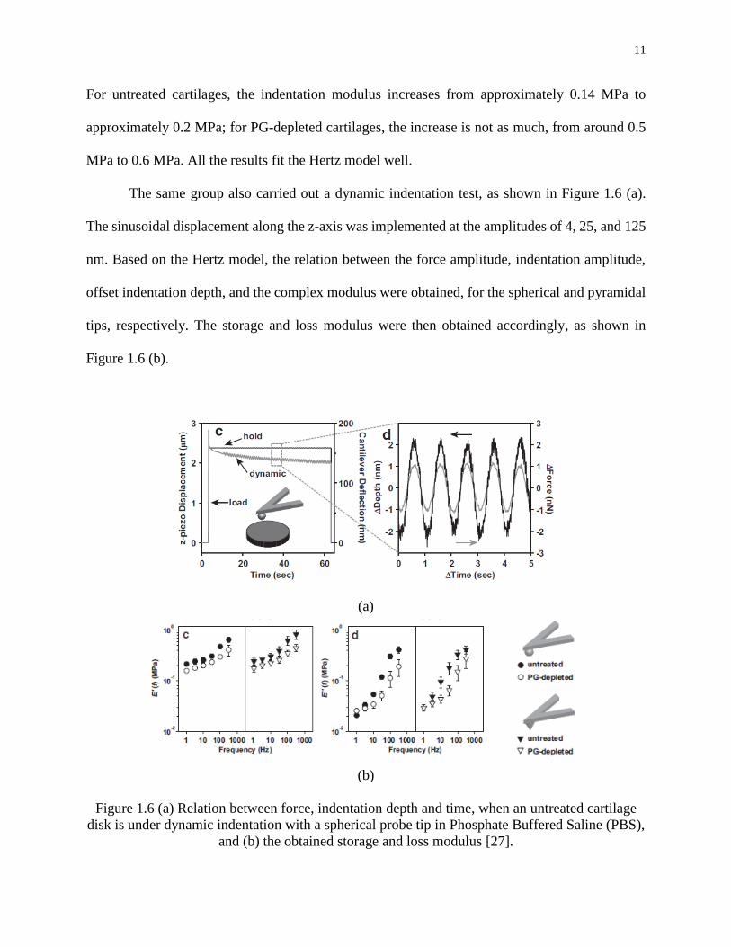
1.6 (a) Relation between force, indentation depth and time, when an untreated cartilage
disk is under dynamic indentation with a spherical probe tip in Phosphate Buffered
Saline (PBS), and (b) the obtained storage and loss modulus [27]. ........................................ 11
1.7 Structure of a V-shaped thermal actuator array [43]. ............................................................. 13
1.8 Schematic of a tactile force sensor that can detect force location [44]. .................................. 13
1.9 Schematic and photo of a piezoresistive-based tactile sensor aiming for minimally
invasive surgery [45]............................................................................................................... 14
1.10 Schematic of a resonator device for in vivo measurement of regional tissue
viscoelasticity [46]. ................................................................................................................. 15
1.11 Material elastic property measurement of a specimen using a microfluidic device [47]. .... 16
1.12 (a) Quantifying the elastic property of a testing sample and (b) quantifying the
transient strain response of a 2% gellan gum and an S. epidermidis biofilm [47]. ................ 16
1.13 Schematic of a MEMS resonant sensor to characterize the viscoelastic properties of
hydrogels [48]. ........................................................................................................................ 17
1.14 Schematic of a MEMS microgripper for measuring the viscoelastic properties of soft
hydrogel microcapsules [49]. .................................................................................................. 18
1.15 Schematic of a spherical cell being grabbed by flat clippers, where the Hertz model is
also applied [49]. ..................................................................................................................... 20
2.1 Schematic view of the microfluidic force sensor. ................................................................... 24
2.2 One sensing segment of the microfluidic device for distributed force sensing (a) side
view of the segment (b) deformation of the polymer structure (c) geometry change of
the electrolyte and its corresponding resistance change. ........................................................ 26
2.3 Photos of (a) a cylindrical probe [60] and (b) a rectangular probe. ........................................ 28
2.4 The circuit configuration and signal flow of the microfluidic device for obtaining a DC
voltage output.......................................................................................................................... 29
xiii
Figure Page
2.5 Simulation result of the displacement field at the y direction for (a) device #1 with a
thinner PDMS structure and (b) device #2 with a thicker PDMS structure (A and B
represent the displacement applied by the probe, and A’ and B’ represent the
microchannel top deformation.). ............................................................................................. 33
2.6 Simulation result of the deformation of the microchannel top under different
indentation depth applied by a rigid probe for both devices. .................................................. 34
2.7 Simulation result of the relation between the reaction force and the indentation depth
under a rigid probe for both devices. ...................................................................................... 35
2.8 Simulation result of the relation between the resistance and indentation depth of one
sensing segment for both devices. .......................................................................................... 36
2.9 Simulation result of the relation between the voltage output and indentation depth of
one sensing segment for both devices. .................................................................................... 36
2.10 Deformation of the microchannel top of one sensing segment of the large microfluidic
device when the indentation depth is 100 μm. ........................................................................ 37
2.11 Mask design for (a) the microchannel and (b) the patterned electrodes. .............................. 38
2.12 Schematics of (a) an SU-8 mold for making the microchannel and two reservoirs on a
Pyrex slide, and (b) electrodes patterning with S1800 photoresist on another Pyrex
slide. ........................................................................................................................................ 39
2.13 Au/Cr electrodes on the Pyrex slide by sputtering and metal deposition. ............................ 40
2.14 SU-8 mold of the microchannel being covered by the 10:1 PDMS mixture cured at
room temperature. ................................................................................................................... 41
2.15 Fabricated microfluidic device with electrolyte in the microchannel. .................................. 42
2.16 Relation between (a) force and indentation depth and (b) voltage output from five
transducers and indentation depth of device #1 (large device). .............................................. 43
2.17 Relation between (a) force and indentation depth and (b) voltage output from five
transducers and indentation depth of device #2 (small device). ............................................. 44
2.18 (a) Schematic of the z-direction misalignment of a probe (front view) and (b)
simulation result of microchannel top deformation of device #1 under the z-direction
misalignment of the probe, when the applied displacement equals to 60 μm. ....................... 47
2.19 (a) Schematic of the in-plane misalignment of the probe (top view) and (b) the effect
of the in-plane misalignment on the microchannel top deformation under 60 μm
prescribed displacement. ......................................................................................................... 48
2.20 Schematic of the misalignment about the x-axis (side view). .............................................. 48
2.21 Schematic of a device with variations in microchannel height (front view). ....................... 49
2.22 Initial voltages of the device output measured within one week. ......................................... 51
2.23 Voltage output of the device at its vibration equilibrium point measured during one
dynamic test. ........................................................................................................................... 51
xiv
Figure Page
3.1 Schematic of a flat sheet under the indentation of a cylinder. ................................................ 55
3.2 A finite element model for verifying the relation between the reaction force and the
indentation depth exerted by a cylinder. ................................................................................. 56
3.3 Theoretical and FEA simulation results of the contact model of a cylinder and a flat
sheet with infinite thickness. ................................................................................................... 57
3.4 Simulation results of force-indentation depth relation with different sheet thicknesses. ....... 58
3.5 The relation between the correction factor α and the thickness of a flat sheet. ...................... 59
3.6 Schematic of the side view of one piece of soft material under indentation applied by a
cylindrical probe. .................................................................................................................... 60
3.7 Rationale of the CSM technique for the elastic modulus measurement. ................................ 61
3.8 Simulation of a piece of heterogeneous material under the indentation applied by a
cylindrical probe on a microfluidic force sensor. ................................................................... 63
3.9 Simulated microchannel top deformation when a piece of homogeneous material is
under the indentation applied by a cylinder probe on the microfluidic device (The
dashed lines represent the locations of the transducers). ........................................................ 64
3.10 Simulated microchannel top deformation when a piece of heterogeneous material
under compression by a cylinder probe on the microfluidic force sensor (The dashed
lines represent the locations of the transducers). .................................................................... 65
3.11 Simulation of a piece of material sample with a hard sphere (r = 1.2 mm) embedded,
indented by a cylindrical probe on the microfluidic device. ................................................... 65
3.12 Deformation of the microchannel top along the microchannel length, when the
distance between the embedded sphere and the device surface increases (The dashed
lines represent the locations of the transducers). .................................................................... 66
3.13 Deformation of the microchannel top along the microchannel length, when the radius
of the embedded sphere increases (The dashed lines represent the locations of the
transducers). ............................................................................................................................ 67
3.14 Deformation of the microchannel top along the microchannel length, when the
Young’s modulus of the embedded sphere increases (The dashed lines represent the
locations of the transducers). .................................................................................................. 68
4.1 Experimental setup for conducting concurrent spatial mapping. ............................................ 71
4.2 A polymer-based microfluidic device with 30 mm microchannel length and a PDMS
container to accommodate materials needing to be tested in an aqueous condition [80]. ...... 71
4.3 Prepared (a) 1:30 homogeneous PDMS (b) 1:30 heterogeneous PDMS and (c) 1:40
heterogeneous PDMS samples [80]. ....................................................................................... 73
4.4 Displacement pattern of the probe for conducting device characterization. ........................... 75
4.5 Flow chart of the data processing procedure of the CSM of the elastic modulus of soft
materials. ................................................................................................................................. 76
xv
Figure Page
4.6 Force and indentation depth relation of the 1:30 homogeneous PDMS sample and the
fitting curves. .......................................................................................................................... 79
4.7 Force and indentation depth relation of the 1:40 heterogeneous PDMS sample and the
fitting curves. .......................................................................................................................... 80
4.8 Measured elastic modulus of the homogeneous (a) 1% agar, (b) 2% agar, and (c) 3%
agar samples as a function of indentation depth. .................................................................... 82
4.9 Measured elastic modulus of the heterogeneous (a) 1% agar, (b) 2% agar, and (c) 3%
agar samples as a function of the indentation depth. .............................................................. 85
5.1 Illustration of phase shifts between stress and strain of (a) purely elastic material, (b)
viscous material and (c) viscoelastic material under harmonic excitation. ............................ 89
5.2 Schematic of the rationale for measuring the heterogeneous viscous behavior of a piece
of soft material. ....................................................................................................................... 90
5.3 (a) Schematic of the side view of a microfluidic device under external sinusoidal
loading, and (b) a second-order mechanical system model of the polymer-based
microfluidic device under a sinusoidal excitation. ................................................................. 91
5.4 (a) Schematic of the side view of a piece of soft material under the dynamic
measurement, and (b) a second-order mechanical system model of a piece of soft
material under a dynamic measurement. ................................................................................ 93
6.1 Experimental setup.................................................................................................................. 97
6.2 A microfluidic device used in the loss modulus measurement of soft materials through
CSM. ....................................................................................................................................... 98
6.3 Schematic of the experimental setup and signal flow for the loss modulus measurement
of soft materials through CSM. ............................................................................................... 99
6.4 Photos of the samples: (a) dragon skin 10, (b) dragon skin 20, (c) Ecoflex, (d) dragon
skin FX-Pro, (e) the first 1:30 PDMS sample with heterogeneity inside, and (f) the
second 1:30 PDMS sample with heterogeneity inside. ......................................................... 101
6.5 Phase and the amplitude ratio obtained from the dynamic characterization of the system
with the setup and the microfluidic device. .......................................................................... 105
6.6 Dynamic stiffness of the system as a function of ω2. ........................................................... 106
6.7 Dynamic damping of the system as a function of ω. ............................................................ 106
6.8 Dynamic measurement results of (a) phase and frequency relation, and (b) compliance
and frequency relation of the dynamic system with Dragon Skin 10. .................................. 108
6.9 Calculated loss modulus of the testing materials. ................................................................. 112
6.10 Phase shift between the force and the voltage output from the device with a 0.75 mm
transducer spacing, when (a) heterogeneous 1:30 PDMS sample1, (b) heterogeneous
1:30 PDMS sample2 are tested. ............................................................................................ 113
6.11 Frequency response of the free vibration of the shaker and probe. .................................... 117

xvi
Figure Page
7.1 Conceptual drawings of (a) a portable force sensor with distributed force sensing
element [44] and (b) conventional forceps mounted with a soft tactile sensor array
[101]. ..................................................................................................................................... 123
A.1 Voltage output from the disptance sensor. ........................................................................... 132
C.1 Setup for conducting dynamic calibration of the load cell. .................................................. 136
D.1 Configuration of the circuits. ............................................................................................... 138
E.1 Experimental setup for measuring the spatially-varying phase shifts. ................................. 140
E.2 Control experiment data in time domain at 10 Hz (The dashed lines show the phase lag
between the applied force and the voltage output). .............................................................. 143
E.3 Measured phase shift between the load input and the voltage outputs of the device as a
function of frequency. ........................................................................................................... 144
E.4 Relation between phase shift and frequency of a 1:30 homogeneous PDMS sample.......... 145
E.5 Relation between phase shift and frequency of a 1:40 homogeneous PDMS sample.......... 146
E.6 Relation between phase shift and frequency of a 1% agar sample. ..................................... 146
E.7 Relation between phase shift and frequency of a 2% agar sample. ..................................... 147
E.8 Relation between phase shift and frequency of a 3% agar sample. ..................................... 147
E.9 Relation between phase shift and frequency of a 1:30 heterogeneous PDMS sample. ....... 148
E.10 Relation between phase shift and frequency of a 1:40 heterogeneous PDMS sample. ..... 149
E.11 Relation between phase shift and frequency of a 1% heterogeneous agar sample. .......... 149
E.12 Relation between phase shift and frequency of a 2% heterogeneous agar sample. ........... 150
E.13 Relation between phase shift and frequency of a 3% heterogeneous agar sample. ........... 150
F.1 LabVIEW block diagram for (a) controlling the micromanipulator to apply different
levels of indentation depth to material samples and (b) the data collection. ........................ 153
F.2 LabVIEW block diagram for the shaker control to achieve constant vibration
amplitude............................................................................................................................... 154
1
CHAPTER 1
INTRODUCTION
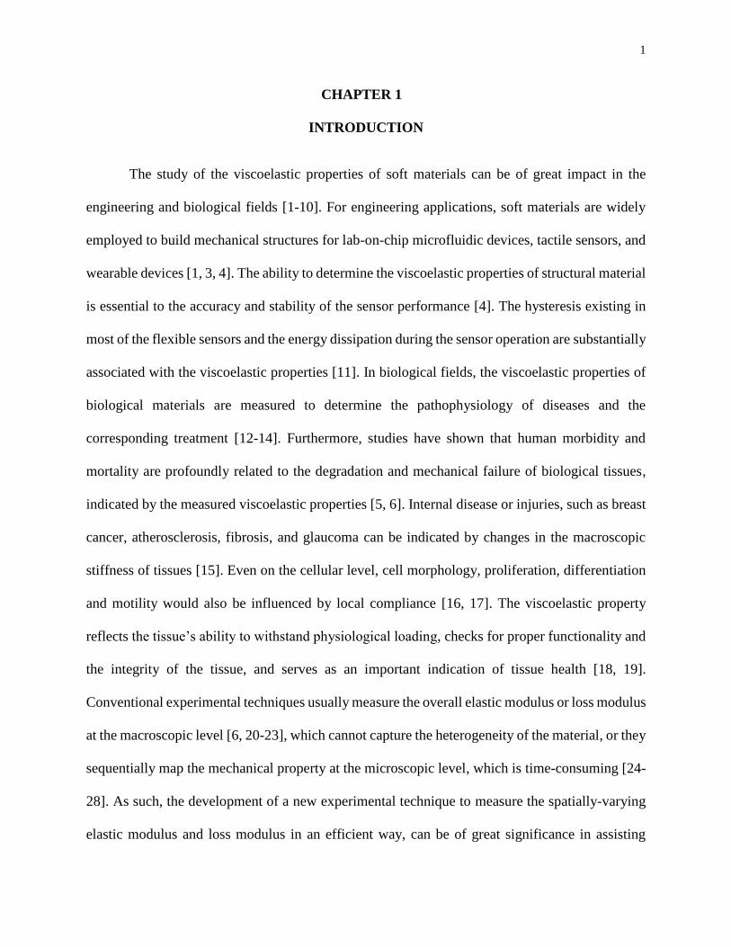
The study of the viscoelastic properties of soft materials can be of great impact in the
engineering and biological fields [1-10]. For engineering applications, soft materials are widely
employed to build mechanical structures for lab-on-chip microfluidic devices, tactile sensors, and
wearable devices [1, 3, 4]. The ability to determine the viscoelastic properties of structural material
is essential to the accuracy and stability of the sensor performance [4]. The hysteresis existing in
most of the flexible sensors and the energy dissipation during the sensor operation are substantially
associated with the viscoelastic properties [11]. In biological fields, the viscoelastic properties of
biological materials are measured to determine the pathophysiology of diseases and the
corresponding treatment [12-14]. Furthermore, studies have shown that human morbidity and
mortality are profoundly related to the degradation and mechanical failure of biological tissues,
indicated by the measured viscoelastic properties [5, 6]. Internal disease or injuries, such as breast
cancer, atherosclerosis, fibrosis, and glaucoma can be indicated by changes in the macroscopic
stiffness of tissues [15]. Even on the cellular level, cell morphology, proliferation, differentiation
and motility would also be influenced by local compliance [16, 17]. The viscoelastic property
reflects the tissue’s ability to withstand physiological loading, checks for proper functionality and
the integrity of the tissue, and serves as an important indication of tissue health [18, 19].
Conventional experimental techniques usually measure the overall elastic modulus or loss modulus
at the macroscopic level [6, 20-23], which cannot capture the heterogeneity of the material, or they
sequentially map the mechanical property at the microscopic level, which is time-consuming [24-
28]. As such, the development of a new experimental technique to measure the spatially-varying
elastic modulus and loss modulus in an efficient way, can be of great significance in assisting
2
material selection in the engineering field and tissue health diagnosis in the biological field.
1.1 Methods for the Measurement of Viscoelastic Properties of Soft Materials
Various experimental techniques have been developed to measure the viscoelastic
properties of soft materials, at both the macroscopic and microscopic levels [15, 21, 24-32].
1.1.1 Methods for the viscoelastic property measurement at the macroscopic level
The Pulse Wave Velocity (PWV) method is an approach commonly used for measuring
arterial stiffness and elastic modulus. The velocity of a pulse wave traveling in the vascular wall
is measured and used to estimate the elastic modulus of the vascular wall [21]. Scanning Acoustic
Microscopy (SAM) is a method that maps the elastic modulus of isolated cells and whole tissues,
but it is limited to hard biological tissues, such as dentin and bone [6]. Magnetic Resonance
Elastography (MRE) is another approach to characterize the mechanical property of tissues [20,
22]. Similarly, the Shearwave Dispersion Ultrasound Vibrometry (SDUV) determines the elastic
modulus and loss modulus of tissues, by detecting the local deformation of tissues under a
harmonic mechanical excitation of shear waves with frequencies up to 1000 Hz [23].
One major category of techniques for measuring the viscoelastic property of soft materials
is through mechanical approaches. Krouskop et al. [29] investigated the viscoelastic behavior of
breast and prostate tissue samples. A hydraulic testing machine was used to apply a uniaxial
compressive sinusoidal load to the sample, and a load cell was assembled to measure the applied
force. This study proved that breast fat tissue has a constant modulus regardless of the strain level,
while the modulus of other tissues is dependent on the strain level. At a high strain level,
carcinomas from the breast were found to be stiffer than the glandular and fibrous tissues.
Similarly, cancerous prostate tissue exhibited the same pattern. The analytical model used in their
research is based on a uniform load acting on a semi-infinite elastic solid. Kim et al. [33] measured
3
the compressive stiffness and radial streaming potential of a cartilage disk under dynamic
compression loading in an unconfined compression chamber.
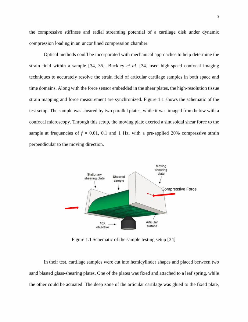
Optical methods could be incorporated with mechanical approaches to help determine the
strain field within a sample [34, 35]. Buckley et al. [34] used high-speed confocal imaging
techniques to accurately resolve the strain field of articular cartilage samples in both space and
time domains. Along with the force sensor embedded in the shear plates, the high-resolution tissue
strain mapping and force measurement are synchronized. Figure 1.1 shows the schematic of the
test setup. The sample was sheared by two parallel plates, while it was imaged from below with a
confocal microscopy. Through this setup, the moving plate exerted a sinusoidal shear force to the
sample at frequencies of f = 0.01, 0.1 and 1 Hz, with a pre-applied 20% compressive strain
perpendicular to the moving direction.
Figure 1.1 Schematic of the sample testing setup [34].
In their test, cartilage samples were cut into hemicylinder shapes and placed between two
sand blasted glass-shearing plates. One of the plates was fixed and attached to a leaf spring, while
the other could be actuated. The deep zone of the articular cartilage was glued to the fixed plate,
Compressive Force
4
and the surface was attached to the moving one. A photo-bleached sample was imaged by a Zeiss
LSM 5 confocal microscopy with 20X magnification. Unstained samples were imaged with a Zeiss
LSM 710 microscope along with a 488-nm laser for illumination. It was demonstrated that
viscoelastic properties of articular cartilage vary drastically with depth, showing a location
dependent mechanical property.
1.1.2 Instrument indentation methods for the measurement of viscoelastic behavior of
materials at the microscopic level
The aforementioned methods all measure the viscoelastic properties at a macroscopic level.
In a macroscopic testing, strain fields usually span the entire sample. Another mechanical approach
that is commonly used for sample viscoelastic properties measurement is based on the force-
deformation response through indentation at the microscopic level [24, 26-28, 36]. Different from
the macroscopic testing, indentation induced deformation only concentrates at the point where the
indenter contacts the sample and gradually diminishes with the increasing distance from the
indenter.
For the indentation type technique, a variety of instruments have been used for material
indentation, ranging from atomic force microscope (AFM), and nanoindenters to larger industrial
indenters. An AFM can apply loads as small as piconewton, nanoindenters can resolve nanonewton
loads, while larger industrial indenters have a more flexible load range, from micronewtons to
meganewtons. Depending on the material type and the specific research objective, different
indentation methods are selected accordingly. Under an elastic deformation assumption, with the
purpose of extracting the elastic modulus, it is crucial to fit the relation between the measured
indentation depth and the indentation load, which is geometry specific [15, 30]. Due to its
consistent and versatile procedure, instrumented nanoindentation has been used to quasi-statically
5
characterize the mechanical properties of a wide range of biological tissues, such as cartilage,
enamel, vascular tissues and sclera [31]. In recent decades, dynamic indentation tests have been
developed to better characterize the material properties, especially for measuring the loss modulus
of materials. McLeod et al. [37] obtained the depth and directional dependence of the microscale
biomechanical properties of porcine cartilage in situ via an AFM. Franke et al. [26] carried out a
dynamic nanoindentation of articular porcine cartilage in vitro and compared the results at different
load amplitudes over the same frequency range. With the development of these techniques,
abnormal tissues are better studied. For example, musculoskeletal diseases on weight-bearing
tissues are better understood based on the elastic modulus obtained with the help of nanoscale
testing techniques [38].
The Atomic Force Microscope (AFM) was invented in 1986 by Binnig et al. [39].
Instrumental improvements and novel applications of AFM have developed rapidly over the last
two decades. AFM has gradually become one of the most useful tools for studying local surface
interactions as a Scanning Probe Microscope (SPM).
Figure 1.2 schematically illustrates the working principle of an atomic force microscope.
The basic structural component for conducting the indentation via an AFM is a flexible cantilever
with a microfabricated sharp tip. The tip will interact with sample surfaces during the
measurement, and the other end of the cantilever is fixed to a holder. During the test, a laser beam
is emitted from a laser diode onto the back surface of the cantilever, right above the tip. The laser
beam is then reflected to a position-sensitive photodiode where the laser spot on the photodiode
moves proportionally to the cantilever deflection. Assuming a constant stiffness of the cantilever,
the interaction force between the tip and the sample can be obtained by multiplying the stiffness

6
with the deflection. The sample is mounted on a piezoelectric scanner in the illustration above and
can move along the x, y and z directions [40].
Figure 1.2 Schematic illustration of the AFM scanning process.
Figure 1.3 illustrates the deformation of a sample and the cantilever during an indentation
test. As illustrated in Figure 1.3, the sphere represents the tip of an AFM’s cantilever. From Figure
1.3, it can be seen that the entire translation of the beam ∆z equals the summation of the cantilever
deflection ∆d and the indentation depth δ [25]. ∆z can be precisely controlled by the piezoelectric
scanner, while ∆d is recorded by the photodiode. As such, the indentation depth on a sample is
easily to be obtained by Equation 1.1:
dz ( 1.1 )
where ∆d can be further used to calculate the interaction force through F=k·∆d, where k is the
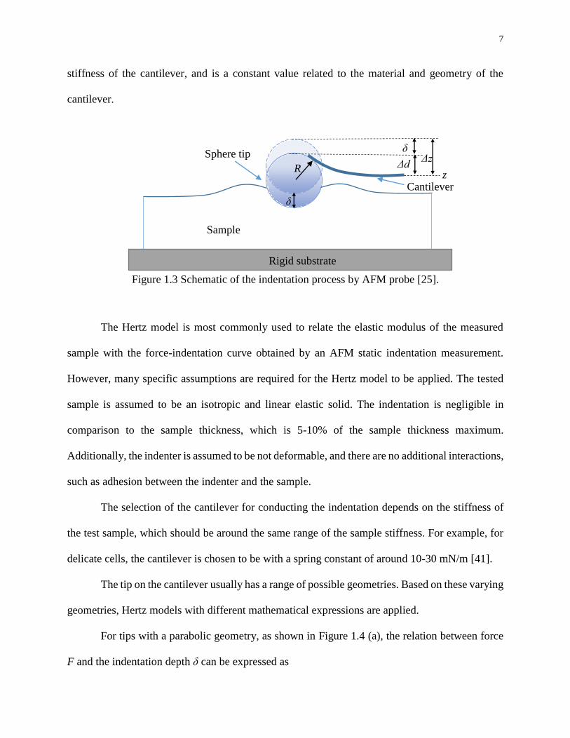
7
stiffness of the cantilever, and is a constant value related to the material and geometry of the
cantilever.
Figure 1.3 Schematic of the indentation process by AFM probe [25].
The Hertz model is most commonly used to relate the elastic modulus of the measured
sample with the force-indentation curve obtained by an AFM static indentation measurement.
However, many specific assumptions are required for the Hertz model to be applied. The tested
sample is assumed to be an isotropic and linear elastic solid. The indentation is negligible in
comparison to the sample thickness, which is 5-10% of the sample thickness maximum.
Additionally, the indenter is assumed to be not deformable, and there are no additional interactions,
such as adhesion between the indenter and the sample.
The selection of the cantilever for conducting the indentation depends on the stiffness of
the test sample, which should be around the same range of the sample stiffness. For example, for
delicate cells, the cantilever is chosen to be with a spring constant of around 10-30 mN/m [41].
The tip on the cantilever usually has a range of possible geometries. Based on these varying
geometries, Hertz models with different mathematical expressions are applied.
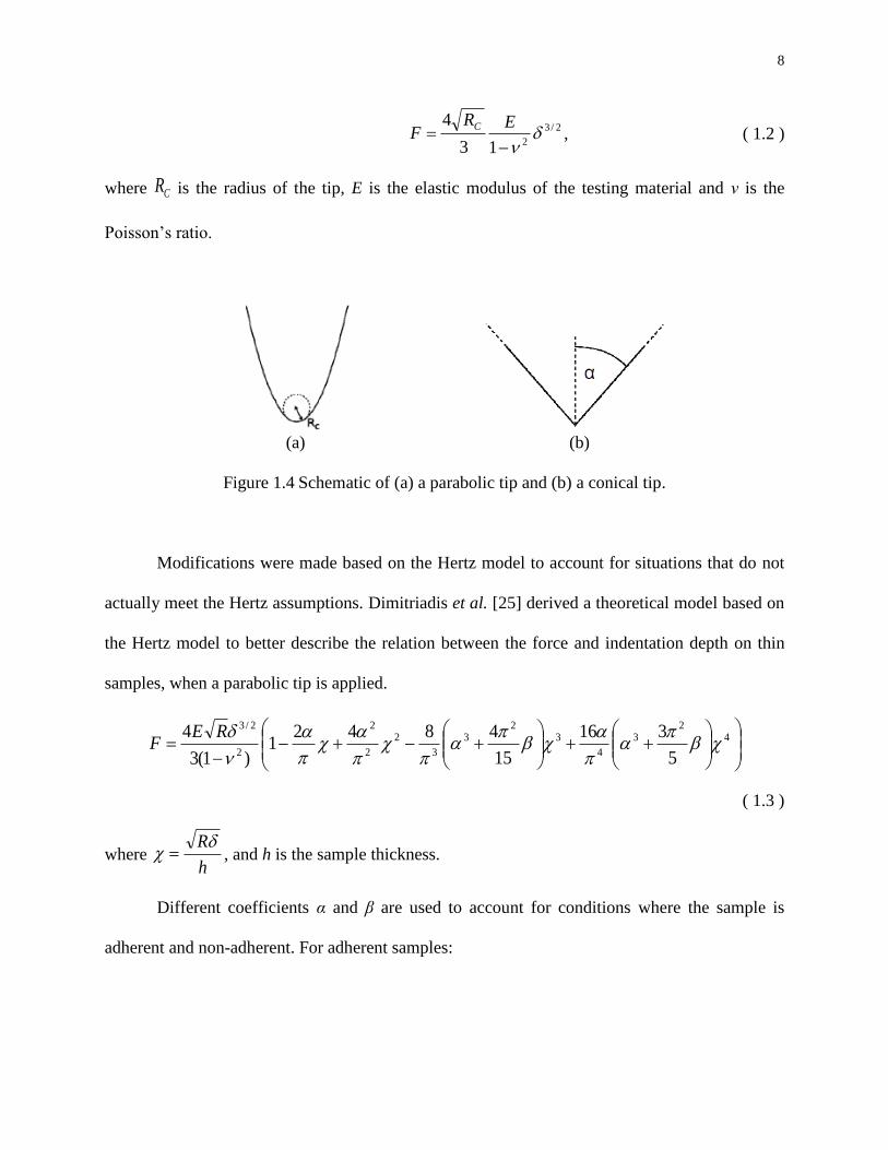
For tips with a parabolic geometry, as shown in Figure 1.4 (a), the relation between force
F and the indentation depth δ can be expressed as
Rigid substrate
R
δ
Δd Δz
δ
z
Sphere tip
Sample
Cantilever
8
2/3
213
4
ERF
C, ( 1.2 )
where CR is the radius of the tip, E is the elastic modulus of the testing material and ν is the
Poisson’s ratio.
(a) (b)
Figure 1.4 Schematic of (a) a parabolic tip and (b) a conical tip.
Modifications were made based on the Hertz model to account for situations that do not
actually meet the Hertz assumptions. Dimitriadis et al. [25] derived a theoretical model based on
the Hertz model to better describe the relation between the force and indentation depth on thin
samples, when a parabolic tip is applied.
4
23
4
32
3
3
2
2
2
2
2/3
5
316
15
48421
)1(3
4
REF
( 1.3 )
where h
R , and h is the sample thickness.
Different coefficients α and β are used to account for conditions where the sample is
adherent and non-adherent. For adherent samples:
9
1
25056.0
1
23347.0
, ( 1.4 )
and for non-adherent samples:
1
5164.10277.16387.0
1
3442.14678.12876.1
2
2
. ( 1.5 )
For conical tips, as shown in Figure 1.4 (b), the force can be derived to be:
2
2
tan2
1
EF ( 1.6 )
where α is the semi-opening angle of the cone.
Similarly, improvements were made to the model to make it applicable to more
complicated situations. Gavara et al. [42] derived a model to account for samples with a small
thickness that are indented by a conical tip.
2
2
22
2
2 tan16
tan21
3
tan8
hh
EF ( 1.7 )
where β is 1.7795 or 0.388 for adherent or non-adherent cases, respectively.
Other than the geometries mentioned above, tips with other geometries are also commonly
used for the cantilever tip of an AFM. The geometry could be a pyramid, hyperboloid, blunt cone,
blunt pyramid, truncated cone and truncated pyramid, etc. The choice of the indenter shape
depends on the mechanical property of the material under measurement. For soft biological
samples with a low elasticitic modulus, spherical probes are recommended, since the stress caused
by the indenter will not be able to damage delicate samples. However, this type of tip may not be
able to obtain high-resolution results. In this case, sharp tips, such as pyramidal silicon nitride tips,
are
10
employed because of their smaller contact dimension. However, sample penetration that will lead
to inaccurate calculation should be avoided [41].
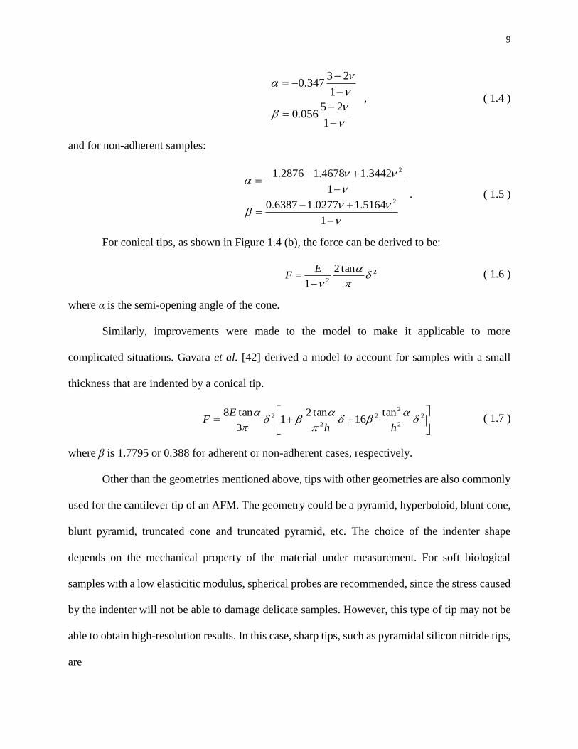
Han et al. [27] carried out an AFM-based classical nanoindentation in Phosphate Buffered
Saline (PBS), using a maximum load of approximately 70 nN in the force mode. The closed looped
control system in the z-direction enabled the precise control of both the indentation force and
depth. Constant displacement rates of 0.1-10 µm/s along the z-axis were used. For each indentation
curve, indentation force-depth relation data were obtained, as can be seen in Figure 1.5. Three
cartilage disk samples, proteoglycan (PG)-depleted and untreated, were tested with both spherical
and pyramidal probe tips. All the indentations were performed at different locations in relatively
flat regions. At each location, the indentation was repeated, and between each repeat, the sample
was rested until recovery.
Figure 1.5 Force-indentation depth curves taken from PG-depleted and untreated cartilages using
two different tips for the AFM-based nanoindentation [27].
From the testing results of the classical indentation, it is noted that the indentation modulus
E increases significantly with the increment of the displacement rate, regardless of the tip type.
11
For untreated cartilages, the indentation modulus increases from approximately 0.14 MPa to
approximately 0.2 MPa; for PG-depleted cartilages, the increase is not as much, from around 0.5
MPa to 0.6 MPa. All the results fit the Hertz model well.
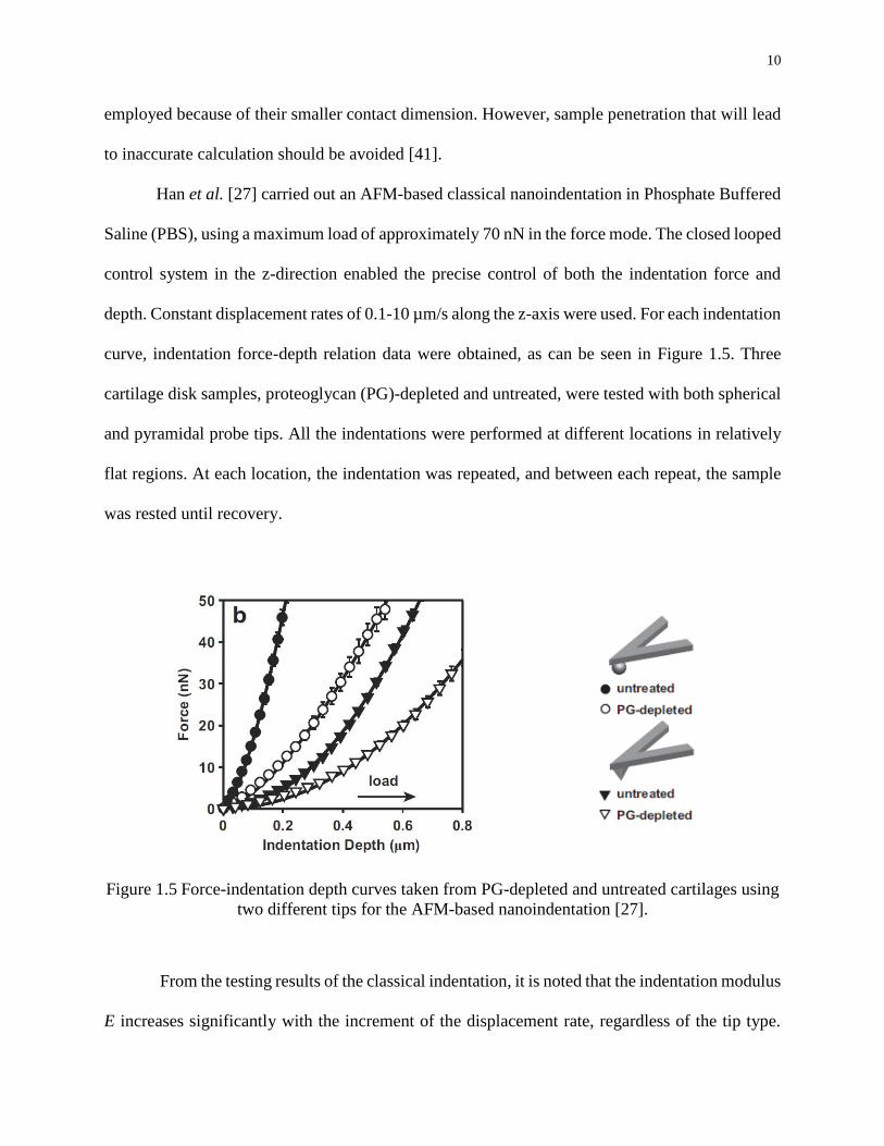
The same group also carried out a dynamic indentation test, as shown in Figure 1.6 (a).
The sinusoidal displacement along the z-axis was implemented at the amplitudes of 4, 25, and 125
nm. Based on the Hertz model, the relation between the force amplitude, indentation amplitude,
offset indentation depth, and the complex modulus were obtained, for the spherical and pyramidal
tips, respectively. The storage and loss modulus were then obtained accordingly, as shown in
Figure 1.6 (b).
(a)
(b)
Figure 1.6 (a) Relation between force, indentation depth and time, when an untreated cartilage
disk is under dynamic indentation with a spherical probe tip in Phosphate Buffered Saline (PBS),
and (b) the obtained storage and loss modulus [27].

12
1.2 Micro/Nano Technology Utilized in the Measurement of the Viscoelastic Properties of
Soft Materials
Although the nanoindentation-based technique exhibits its advantages in measuring the
viscoelastic behavior of a material on a submicrometer scale and is broadly applied in measuring
the elastic modulus of biological materials, it also has drawbacks. For example, this technique only
provides a local mechanical stimulation around 100 nm in depth, which fails to capture the in-
depth mechanical property. The stimulation is also limited by the size of the cantilever tip of an
AFM. The interaction among neighboring compositions in a tissue specimen under physiological
loading is also missing, especially at the tissue level study of biomechanics. Furthermore, the
spatial mapping for a piece of material using AFM is time consuming and costly.
Other mechanical methods based on micro/nano technology have also been explored, due
to their low cost and ability to integrate microsensors on a single chip. Zhang et al. [43] developed
a V-shaped polymer electrothermal actuator array for measuring the mechanical compliance of a
biological cell, as shown in Figure 1.7. The actuation mechanism has an electrothermal effect, as
it enables the device to be operated in a cell medium. Dielectrophoresic quadrupole electrodes are
used to trap a cell between a plunger and a force sensor. Then, the desired strain is applied to the
cell by the V-shaped electrothermal actuator array while the force sensor measures the applied
force. Meanwhile, the temperature during the experiment is monitored by a thermal sensor on the
chip.

13
Figure 1.7 Structure of a V-shaped thermal actuator array [43].
Sokhanvar et al. [44] developed a tactile sensor that is able to measure force, force position,
and the softness of a grasped object, as shown in Figure 1.8. A uniaxial polyvinylidene fluoride
(PVDF) film is used as the transduction element. When soft materials are grasped, the bending of
a PVDF beam generates a voltage signal, which is related to the deformation of the beam and is
further related to the softness of the grasped object. As a drawback of piezoelectric materials, static
loads are not able to be detected. Thus, a dynamic load is applied in the test and the peak-to-peak
voltage value of the PVDF output is further analyzed.
Figure 1.8 Schematic of a tactile force sensor that can detect force location [44].
14
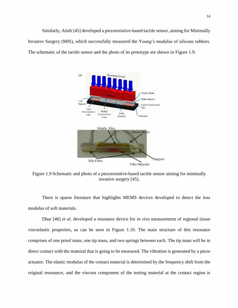
Similarly, Atieh [45] developed a piezoresistive-based tactile sensor, aiming for Minimally
Invasive Surgery (MIS), which successfully measured the Young’s modulus of silicone rubbers.
The schematic of the tactile sensor and the photo of its prototype are shown in Figure 1.9.
Figure 1.9 Schematic and photo of a piezoresistive-based tactile sensor aiming for minimally
invasive surgery [45].
There is sparse literature that highlights MEMS devices developed to detect the loss
modulus of soft materials.
Dhar [46] et al. developed a resonator device for in vivo measurement of regional tissue
viscoelastic properties, as can be seen in Figure 1.10. The main structure of this resonator
comprises of one proof mass, one tip mass, and two springs between each. The tip mass will be in
direct contact with the material that is going to be measured. The vibration is generated by a piezo
actuator. The elastic modulus of the contact material is determined by the frequency shift from the
original resonance, and the viscous component of the testing material at the contact region is
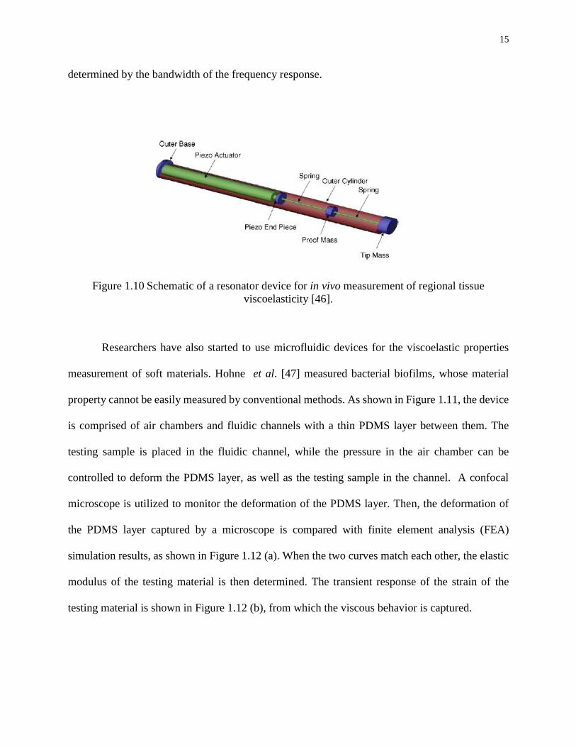
15
determined by the bandwidth of the frequency response.
Figure 1.10 Schematic of a resonator device for in vivo measurement of regional tissue
viscoelasticity [46].
Researchers have also started to use microfluidic devices for the viscoelastic properties
measurement of soft materials. Hohne et al. [47] measured bacterial biofilms, whose material
property cannot be easily measured by conventional methods. As shown in Figure 1.11, the device
is comprised of air chambers and fluidic channels with a thin PDMS layer between them. The
testing sample is placed in the fluidic channel, while the pressure in the air chamber can be
controlled to deform the PDMS layer, as well as the testing sample in the channel. A confocal
microscope is utilized to monitor the deformation of the PDMS layer. Then, the deformation of
the PDMS layer captured by a microscope is compared with finite element analysis (FEA)
simulation results, as shown in Figure 1.12 (a). When the two curves match each other, the elastic
modulus of the testing material is then determined. The transient response of the strain of the
testing material is shown in Figure 1.12 (b), from which the viscous behavior is captured.

16
Figure 1.11 Material elastic property measurement of a specimen using a microfluidic device
[47].
(a)
(b)
Figure 1.12 (a) Quantifying the elastic property of a testing sample and (b) quantifying the
transient strain response of a 2% gellan gum and an S. epidermidis biofilm [47].

17
As shown in Figure 1.13, Corbin et al. [48] developed a MEMS resonant sensor to measure
the viscoelastic properties of hydrogels over a range of concentrations. Gels with different
concentrations were fabricated directly onto the devices using an electrohydrodynamic jet printing
technique. The viscoelastic properties of the material is measured based on the technique of
measuring frequency shift between a sensor without loading a hydrogel and a sensor loaded with
a piece of hydrogel.
Figure 1.13 Schematic of a MEMS resonant sensor to characterize the viscoelastic properties of
hydrogels [48].
Kim et al. [49] reported a MEMS microgripper which integrates two capacitive force
sensors and one electrothermal microactuator on a single chip, as shown in Figure 1.14. The
microgripper is capable of measuring the viscoelastic properties of soft hydrogel microcapsules at
the size of around 15-25 µm. The electrothermal microactuator generates gripping displacements
at the arm tips, while the capacitive force sensors measure the force applied on the microcapsules
and provide a feedback. Meanwhile, the material deformations are measured from phase contrast
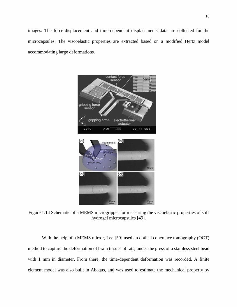
18
images. The force-displacement and time-dependent displacements data are collected for the
microcapsules. The viscoelastic properties are extracted based on a modified Hertz model
accommodating large deformations.
Figure 1.14 Schematic of a MEMS microgripper for measuring the viscoelastic properties of soft
hydrogel microcapsules [49].
With the help of a MEMS mirror, Lee [50] used an optical coherence tomography (OCT)
method to capture the deformation of brain tissues of rats, under the press of a stainless steel bead
with 1 mm in diameter. From there, the time-dependent deformation was recorded. A finite
element model was also built in Abaqus, and was used to estimate the mechanical property by
19
comparing the simulation results with the deformation profile obtained from the optical
measurement.
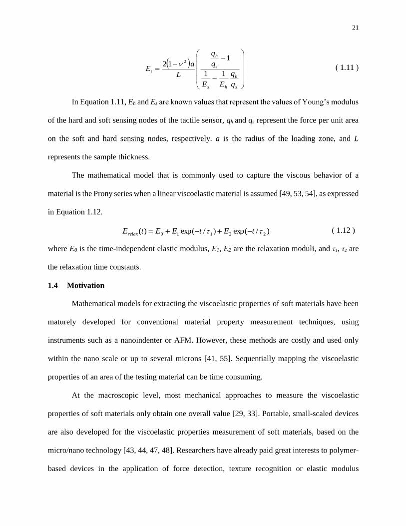
1.3 Mathematical Models for Extracting the Viscoelastic Properties of Materials using
Micro/Nano Technology
The most commonly used mathematical model for extracting the elastic modulus from the
measurement is the Hertz model. The Hertz model is widely used in cellular level material property
measurement using AFM or nanoindentation technique, as mentioned previously [27, 41, 42]. In
the above-mentioned examples, one sample is pressed by a spherical indenter tip. The same
mathematical model is also applied to the scenario of one spherical cell being grabbed by flat
clippers, as can be seen in Figure 1.15. In both cases, the measurement of the force-indentation
relation is needed. From the relation, the elastic modulus of the testing material is calculated using
Equation 1.8.
3
2
4
13
R
FE
( 1.8 )
where F is the measured force, δ is the measured indentation depth, and R is the radius of either
the indenter tip or the spherical cell being grabbed.

20
Figure 1.15 Schematic of a spherical cell being grabbed by flat clippers, where the Hertz model
is also applied [49].
Instead of using the classic Hertz model which only accounts for the force-displacement
relation under small deformation, Kim [49] adopted the model developed by Tatara [51], which
takes large deformation of soft material samples into consideration. As shown in Equations 1.9
and 1.10, higher order terms are added to relate force and deformation. As such, the elastic modulus
of the material is achieved by curve fitting.
E
Faf
Ea
F
)(
4
)1(3 2
( 1.9 )
2/122
2
2/322
2
)4(
1
)4(
)1(2)(
RaRa
Raf
( 1.10 )
where a is the contact radius, δ is the sample deformation, R is the radius of the cell, ν is the
Poisson’s ratio, and F is the force applied on the spherical cell.
Peng [52] developed a theoretical model for extracting the elastic modulus of the testing
materials, based on a MEMS tactile sensor developed by their group. Under the assumption that
the deformation of a sample only occurs over a very small area, Equation 1.11 is developed.
21
s
h
hs
s
h
t
q
q
EE
q
q
L
aE
11
112 2 ( 1.11 )
In Equation 1.11, Eh and Es are known values that represent the values of Young’s modulus
of the hard and soft sensing nodes of the tactile sensor, qh and qs represent the force per unit area
on the soft and hard sensing nodes, respectively. a is the radius of the loading zone, and L
represents the sample thickness.
The mathematical model that is commonly used to capture the viscous behavior of a
material is the Prony series when a linear viscoelastic material is assumed [49, 53, 54], as expressed
in Equation 1.12.
)/exp()/exp()( 22110 tEtEEtErelax ( 1.12 )
where E0 is the time-independent elastic modulus, E1, E2 are the relaxation moduli, and τ1, τ2 are
the relaxation time constants.
1.4 Motivation
Mathematical models for extracting the viscoelastic properties of soft materials have been
maturely developed for conventional material property measurement techniques, using
instruments such as a nanoindenter or AFM. However, these methods are costly and used only
within the nano scale or up to several microns [41, 55]. Sequentially mapping the viscoelastic
properties of an area of the testing material can be time consuming.
At the macroscopic level, most mechanical approaches to measure the viscoelastic
properties of soft materials only obtain one overall value [29, 33]. Portable, small-scaled devices
are also developed for the viscoelastic properties measurement of soft materials, based on the
micro/nano technology [43, 44, 47, 48]. Researchers have already paid great interests to polymer-
based devices in the application of force detection, texture recognition or elastic modulus
22
measurement of soft materials including biological samples [47, 56-58], due to the flexibility of
polymer materials and their biocompatibility. Only a few researchers utilized conductive liquid as
a transduction mechanism. Gutierrez et al. [56] developed an impedance-based force sensor with
a fluid-filled parylene microstructure. However, the nonlinear relations of the force and the device
deflection, as well as the impedance change and the device deflection, caused the inconvenience
in interpreting the data in real applications. Thus, no further quantitative application was discussed.
Only a few of the works achieved a quantitative relation between the viscoelastic properties of the
testing materials and the sensor output [47, 57], let alone quantifying the spatially-varying
mechanical properties with one measurement. Ahmadi et al. [59] reported on a discretely loaded
beam-type optical fiber tactile sensor which is able to detect the existence of a lump in a tissue
specimen, when a tissue specimen is pressed against the sensor. To the best knowledge of the
author, this work is the closest to the concept that to examine the spatially-varying elastic modulus
of a soft material through one single device. However, no quantitative relation between the elastic
property of the testing material and the device output is presented in the work. The miniaturization
and mass production of the sensor is also a challenge, due to the size of the prototype (45 mm × 8
mm × 8 mm). On the other hand, other than measuring the spatially-varying viscoelastic properties
by sequential measurement through the nanoindentation-based technique, no other groups have
studied on measuring the spatially-varying viscoelastic properties through one device in one
measurement.
1.5 Objectives
This work aims to develop a novel experimental technique to measure the spatially-varying
viscoelastic properties of soft materials through a polymer-based microfluidic device developed
for this study.
23
1.6 Dissertation Layout
Chapter Two presents the microfluidic device employed in the CSM in this work. The
working principle and its performance characterization are presented. Technical issues associated
with the device and the CSM technique are also discussed.
Chapter Three presents the theory of the CSM technique for acquiring the spatially-varying
elastic modulus of soft materials.
Chapter Four presents the implementation of the CSM technique on the elastic modulus
measurement of synthetic soft materials. The testing results are presented and compared with those
in the literature. Heterogeneity within a material is also successfully detected.
Chapter Five presents the theory of the CSM technique for acquiring the spatially-varying
viscous property of soft materials. The relation between the loss modulus and the measurable
damping coefficient is also derived.
Chapter Six presents the implementation of the CSM technique for the viscous
measurement of soft materials, including the spatially-varying phase shifts, the overall stiffness,
the damping coefficient, and the frequency-dependent loss modulus.
Finally, Chapter Seven discusses the advantages and drawbacks of the CSM technique, and
proposes future work that can be built upon this dissertation.
24
CHAPTER 2
A POLYMER-BASED MICROFLUIDIC DEVICE FOR DISTRIBUTED-LOAD
DETECTION
This chapter presents a polymer-based microfluidic resistive sensor employed in this study
for the measurement of the viscoelastic properties of soft materials. The sensor is mainly
comprised of a rectangular polymer microstructure and an array of electrolyte-enabled distributed
resistive transducers. Distributed loads deform the polymer microstructure and are recorded as
resistance changes at the locations of the transducers. Since the detailed design, fabrication, and
characterization process of the device have been presented in the previous work [60-62], a brief
introduction of the device is given in this chapter for completeness. Then, the working principle,
input-output relation, and technical issues associated with the microfluidic device and the
experimental technique are elaborated in the rest of the chapter.
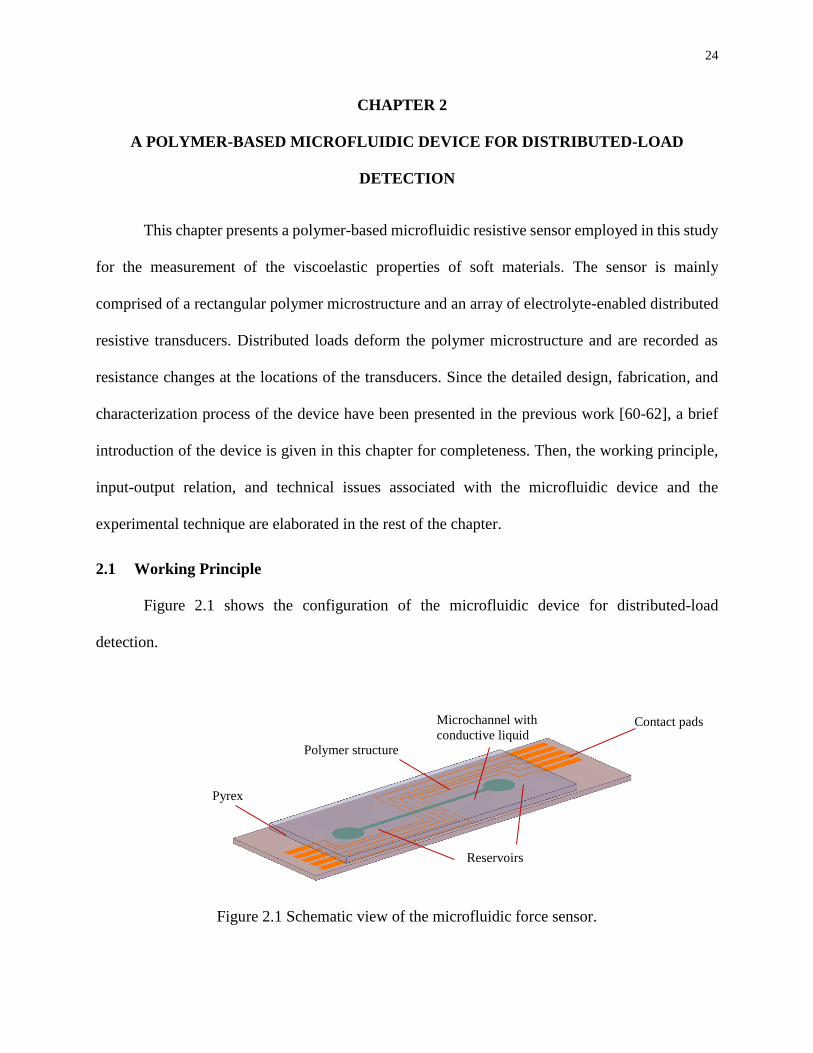
2.1 Working Principle
Figure 2.1 shows the configuration of the microfluidic device for distributed-load
detection.
Figure 2.1 Schematic view of the microfluidic force sensor.
Contact pads
Reservoirs
Polymer structure
Pyrex
Microchannel with
conductive liquid
25
The main structure of the device is a rectangular polymer (Polydimethylsiloxane: PDMS)
microstructure embedded with a microchannel. The microchannel is filled with an electrolyte, 1-
ethyl-3-methylimidazolium dicyanamide (EMIDCA). Five electrode pairs are immersed in the
electrolyte in the microchannel, functioning as five discrete resistive transducers together with the
electrolyte. Two reservoirs, located at the two ends of the microchannel, allow the conductive
liquid to be injected, stored, and to flow in and out during operation. The microstructure converts
distributed normal loads to continuous deflections, which further convert to resistance changes at
the transducer locations. The microchannel length, microchannel width, transducer spacing, and
the polymer structure thickness are the key design parameters and that can be adjusted. The key
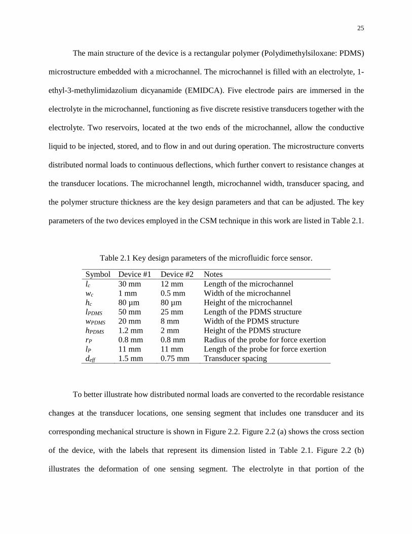
parameters of the two devices employed in the CSM technique in this work are listed in Table 2.1.
Table 2.1 Key design parameters of the microfluidic force sensor.
Symbol Device #1 Device #2 Notes
lc 30 mm 12 mm Length of the microchannel
wc 1 mm 0.5 mm Width of the microchannel
hc 80 µm 80 µm Height of the microchannel
lPDMS 50 mm 25 mm Length of the PDMS structure
wPDMS 20 mm 8 mm Width of the PDMS structure
hPDMS 1.2 mm 2 mm Height of the PDMS structure
rP 0.8 mm 0.8 mm Radius of the probe for force exertion
lP 11 mm 11 mm Length of the probe for force exertion
deff 1.5 mm 0.75 mm Transducer spacing
To better illustrate how distributed normal loads are converted to the recordable resistance
changes at the transducer locations, one sensing segment that includes one transducer and its
corresponding mechanical structure is shown in Figure 2.2. Figure 2.2 (a) shows the cross section
of the device, with the labels that represent its dimension listed in Table 2.1. Figure 2.2 (b)
illustrates the deformation of one sensing segment. The electrolyte in that portion of the
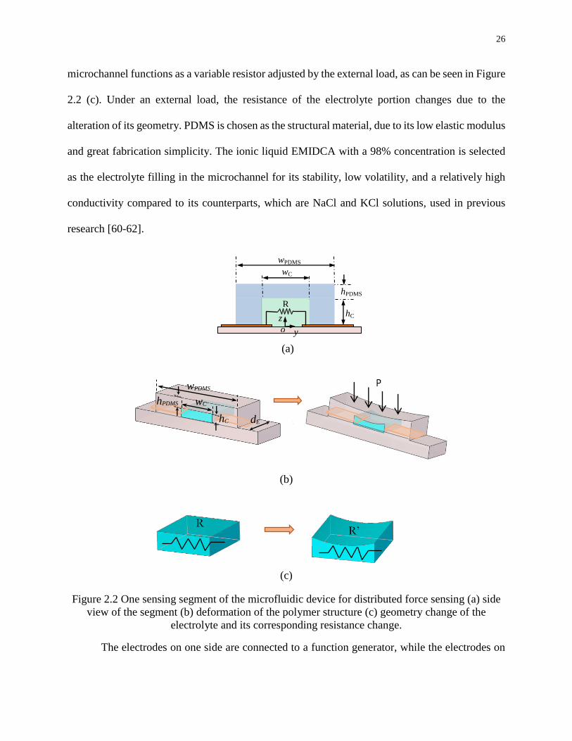
26
microchannel functions as a variable resistor adjusted by the external load, as can be seen in Figure
2.2 (c). Under an external load, the resistance of the electrolyte portion changes due to the
alteration of its geometry. PDMS is chosen as the structural material, due to its low elastic modulus
and great fabrication simplicity. The ionic liquid EMIDCA with a 98% concentration is selected
as the electrolyte filling in the microchannel for its stability, low volatility, and a relatively high
conductivity compared to its counterparts, which are NaCl and KCl solutions, used in previous
research [60-62].
(a)
(b)
(c)
Figure 2.2 One sensing segment of the microfluidic device for distributed force sensing (a) side
view of the segment (b) deformation of the polymer structure (c) geometry change of the
electrolyte and its corresponding resistance change.
The electrodes on one side are connected to a function generator, while the electrodes on
hPDMS
z
y o
R
wPDMS
hC
wC
wPDMS
wC hPDMS
hC dE
27
the other side are connected to the circuits that amplify the signals and convert them to DC output.
The device essentially has both a capacitive and a resistive nature. The capacitive nature is mainly
from the double layer effect formed by the electrode-electrolyte interface. However, with the
highly conductive electrolyte EMIDCA, the entire device can be treated as resistive dominant
when the passing signal is at high frequencies (>100 kHz), since at high frequencies the capacitor
is treated as a wire [61, 63-65]. Besides, DC voltage will cause severe electrolysis and damage the
deposited electrodes. In this work, the voltage of the AC signal is kept around 200 mV. As
mentioned by Gurierrez et al. [66], low voltage magnitude helps prevent the hydrolysis of the
electrolyte. Each opposing pair of electrodes can record the voltage on the electrolyte portion at
its corresponding location. Deflection of the PDMS structure causes a corresponding resistance
change of the electrolyte in the microchannel and is recorded as a change in the output DC voltage.
A device characterization has to be carried out for obtaining the relation between the voltage output
and the mechanical input before conducting any measurement on material samples. Once this
relation is established, the deformation of the PDMS microstructure at the locations of the
transducers can be deduced from the change in the voltage output. A simultaneous spatial
measurement thus becomes feasible.
The mechanical input is applied by a rigid probe. Normally, two types of probes are
utilized, a cylindrical probe and a probe with a rectangular shape, as can be seen in Figure 2.3. The
two types of probes have their own advantages and disadvantages. The cylindrical probe provides
a regional deformation above the microchannel, leaving the rest of the device or the rest region of
the material, under test minimally affected by the applied load. At the same time, due to the
cylindrical shape, misalignment of the probe about its own axis is alleviated. The probe with a
rectangular shape covers a larger region of the device, which will give rise to a larger deformation
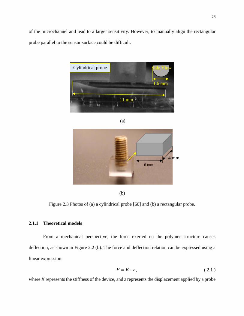
28
of the microchannel and lead to a larger sensitivity. However, to manually align the rectangular
probe parallel to the sensor surface could be difficult.
(a)
(b)
Figure 2.3 Photos of (a) a cylindrical probe [60] and (b) a rectangular probe.
2.1.1 Theoretical models
From a mechanical perspective, the force exerted on the polymer structure causes
deflection, as shown in Figure 2.2 (b). The force and deflection relation can be expressed using a
linear expression:
zKF , ( 2.1 )
where K represents the stiffness of the device, and z represents the displacement applied by a probe
Cylindrical probe
11 mm
6 mm
4 mm
1.6 mm
Side View
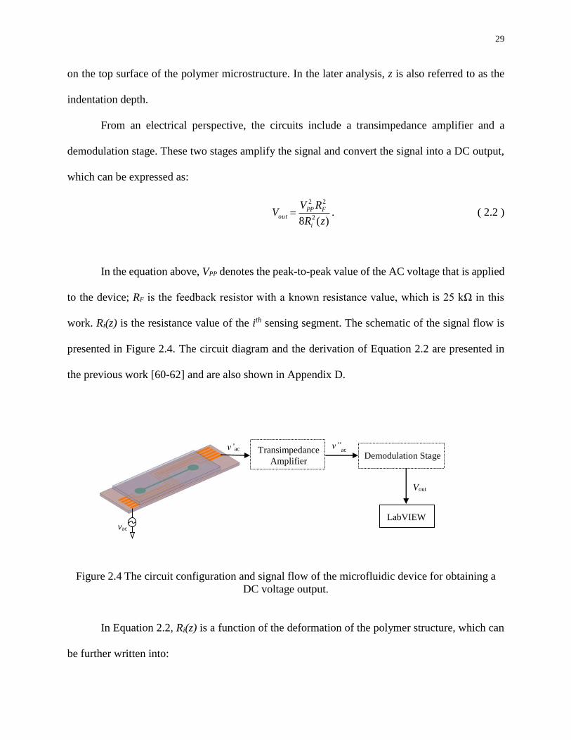
29
on the top surface of the polymer microstructure. In the later analysis, z is also referred to as the
indentation depth.
From an electrical perspective, the circuits include a transimpedance amplifier and a
demodulation stage. These two stages amplify the signal and convert the signal into a DC output,
which can be expressed as:
)(8 2
22
zR
RVV
i
FPPout . ( 2.2 )
In the equation above, VPP denotes the peak-to-peak value of the AC voltage that is applied
to the device; RF is the feedback resistor with a known resistance value, which is 25 kΩ in this
work. Ri(z) is the resistance value of the ith sensing segment. The schematic of the signal flow is
presented in Figure 2.4. The circuit diagram and the derivation of Equation 2.2 are presented in
the previous work [60-62] and are also shown in Appendix D.
Figure 2.4 The circuit configuration and signal flow of the microfluidic device for obtaining a
DC voltage output.
In Equation 2.2, Ri(z) is a function of the deformation of the polymer structure, which can
be further written into:
LabVIEW
Vout
Transimpedance
Amplifier Demodulation Stage
vac
v’ac v”ac
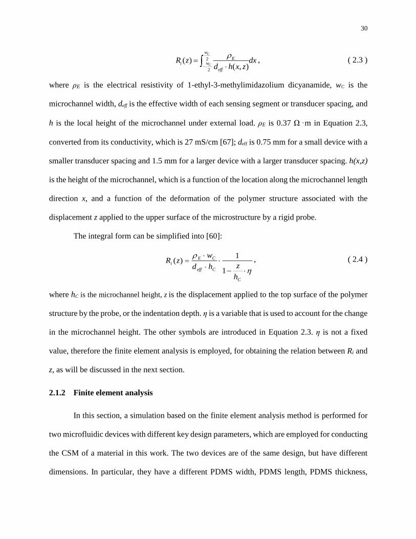
30
2
2
( )( , )
C
C
w
Ewi
eff
R z dxd h x z
, ( 2.3 )
where ρE is the electrical resistivity of 1-ethyl-3-methylimidazolium dicyanamide, wC is the
microchannel width, deff is the effective width of each sensing segment or transducer spacing, and
h is the local height of the microchannel under external load. ρE is 0.37 Ω·m in Equation 2.3,
converted from its conductivity, which is 27 mS/cm [67]; deff is 0.75 mm for a small device with a
smaller transducer spacing and 1.5 mm for a larger device with a larger transducer spacing. h(x,z)
is the height of the microchannel, which is a function of the location along the microchannel length
direction x, and a function of the deformation of the polymer structure associated with the
displacement z applied to the upper surface of the microstructure by a rigid probe.
The integral form can be simplified into [60]:
C
Ceff
CE
i
h
zhd
wzR
1
1)( , ( 2.4 )
where hC is the microchannel height, z is the displacement applied to the top surface of the polymer
structure by the probe, or the indentation depth. η is a variable that is used to account for the change
in the microchannel height. The other symbols are introduced in Equation 2.3. η is not a fixed
value, therefore the finite element analysis is employed, for obtaining the relation between Ri and
z, as will be discussed in the next section.
2.1.2 Finite element analysis
In this section, a simulation based on the finite element analysis method is performed for
two microfluidic devices with different key design parameters, which are employed for conducting
the CSM of a material in this work. The two devices are of the same design, but have different
dimensions. In particular, they have a different PDMS width, PDMS length, PDMS thickness,

31
microchannel width, and transducer spacing. The key design parameters of the two devices are
listed in Table 2.1 for comparison.
For simplicity a 2D model is built in COMSOL Multiphysics 4.4 for each device to study
the relations between the reaction force and the indentation depth, the resistance of each sensing
segment and the indentation depth, and the voltage output of one sensing segment and the
indentation depth. Plane strain is assumed in this simulation. Since the device is symmetric, only
half of the device is included in the 2D model. Other than the main geometric dimensions of the
two devices listed in Table 2.1, the material properties of the devices are shown in Table 2.2.
Table 2.2 Material properties used in the simulation.
Symbol Value Unit Notes
E_PDMS 700 kPa Young’s modulus of PDMS
ν_PDMS 0.45 - Poisson’s ratio of PDMS
ρ_PDMS 1000 kg/m3 Density of PDMS
E_probe 530 GPa Young’s modulus of the probe
ν_probe 0.31 - Poisson’s ratio of the probe
ρ_probe 1560 kg/m3 Density of the probe
E_pyrex 67 GPa Young’s modulus of the substrate
ν_pyrex 0.2 - Poisson’s ratio of the substrate
ρ_pyrex 2230 kg/m3 Density of the substrate
As can be seen in Table 2.1, the two devices used in this work mainly differ in the
microchannel width, the height of the PDMS structure, and the transducer spacing. The
microchannel height is only 80 µm, less than 10% of the total thickness of either of the devices. It
should be noted that the model only includes the solid structure, since the amount of the conductive
liquid is small enough to be considered to have a negligible reaction force to the microstructure
deformation. The two models are built in COMSOL Multiphysics 4.4. For the large device (device

32
#1), 2014 mesh elements are created, while for the small one (device #2) 2921 mesh elements are
created.
Figure 2.5 shows the simulation results for both devices. The displacement fields in the y
direction (along microchannel height) for both devices are presented in Figure 2.5 (a) and (b).
Although the deformation mainly happens near the rigid probe, the microchannel shape still
changes and is able to generate a resistance change in the sensing segment. Figure 2.6 shows the
relation between the deformation of the microchannel top and the indentation depth. The
displacement along the y-direction of points A and B, as can be seen in Figure 2.5 (a) and (b),
represents the displacement applied by the rigid probe on devices #1 and #2, respectively. The
displacement along the y direction of points A’ and B’ represents the deformation of the
microchannel top of the two devices.
Figure 2.6 shows the deformation of the top of the microchannel of both devices under a
prescribed displacement up to 300 μm applied by a rigid cylindrical probe. The deformation of the
microchannel is represented by the displacement of the point located right in the middle of the
microchannel top (A’ and B’ in Figure 2.5). It can be seen that the microchannel of the small device
(device #2) deforms less than the large one (device #1), due to its smaller microchannel width and
larger PDMS structure thickness.
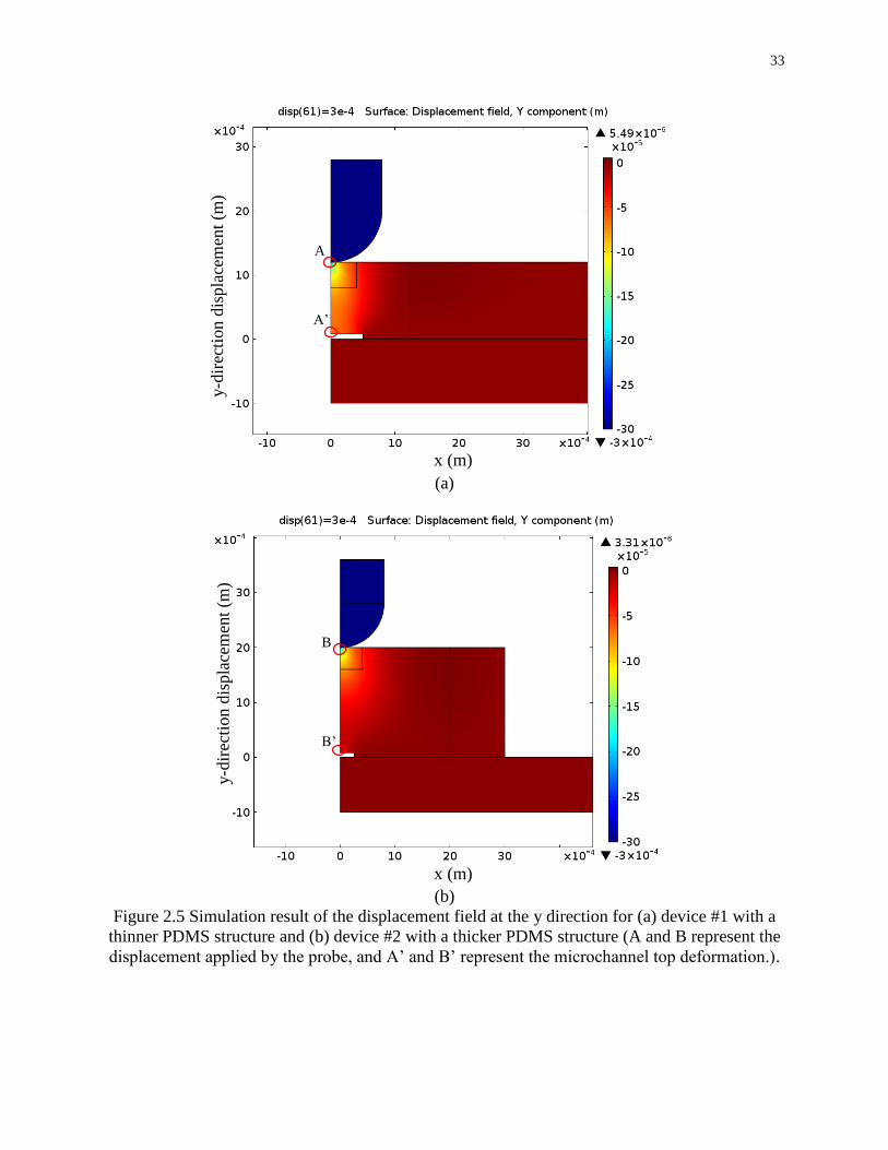
33
(a)
(b)
Figure 2.5 Simulation result of the displacement field at the y direction for (a) device #1 with a
thinner PDMS structure and (b) device #2 with a thicker PDMS structure (A and B represent the
displacement applied by the probe, and A’ and B’ represent the microchannel top deformation.).
A
A’
B’
B
x (m)
y-d
irec
tion d
ispla
cem
ent
(m)
x (m)
y-d
irec
tion d
ispla
cem
ent
(m)
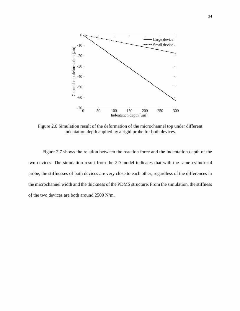
34
Figure 2.6 Simulation result of the deformation of the microchannel top under different
indentation depth applied by a rigid probe for both devices.
Figure 2.7 shows the relation between the reaction force and the indentation depth of the
two devices. The simulation result from the 2D model indicates that with the same cylindrical
probe, the stiffnesses of both devices are very close to each other, regardless of the differences in
the microchannel width and the thickness of the PDMS structure. From the simulation, the stiffness
of the two devices are both around 2500 N/m.
0 50 100 150 200 250 300-70
-60
-50
-40
-30
-20
-10
0
Indentation depth [m]
Ch
ann
el t
op
def
orm
atio
n [
m
]
Large device
Small device
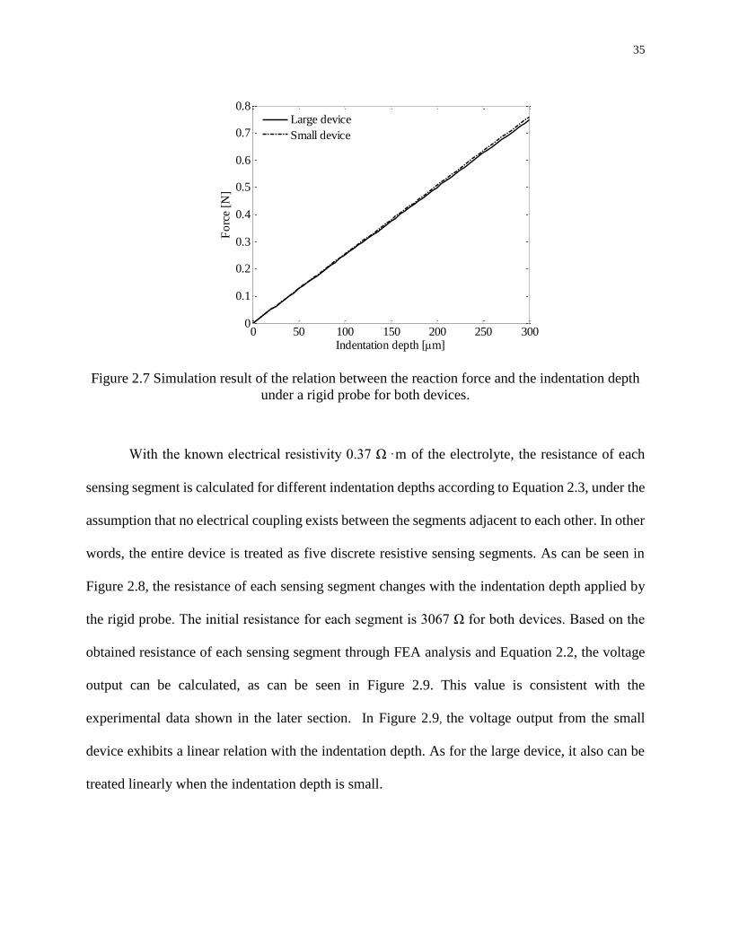
35
Figure 2.7 Simulation result of the relation between the reaction force and the indentation depth
under a rigid probe for both devices.
With the known electrical resistivity 0.37 Ω·m of the electrolyte, the resistance of each
sensing segment is calculated for different indentation depths according to Equation 2.3, under the
assumption that no electrical coupling exists between the segments adjacent to each other. In other
words, the entire device is treated as five discrete resistive sensing segments. As can be seen in
Figure 2.8, the resistance of each sensing segment changes with the indentation depth applied by
the rigid probe. The initial resistance for each segment is 3067 Ω for both devices. Based on the
obtained resistance of each sensing segment through FEA analysis and Equation 2.2, the voltage
output can be calculated, as can be seen in Figure 2.9. This value is consistent with the
experimental data shown in the later section. In Figure 2.9, the voltage output from the small
device exhibits a linear relation with the indentation depth. As for the large device, it also can be
treated linearly when the indentation depth is small.
0 50 100 150 200 250 3000
0.1
0.2
0.3
0.4
0.5
0.6
0.7
0.8
Indentation depth [m]
Fo
rce
[N]
Large device
Small device
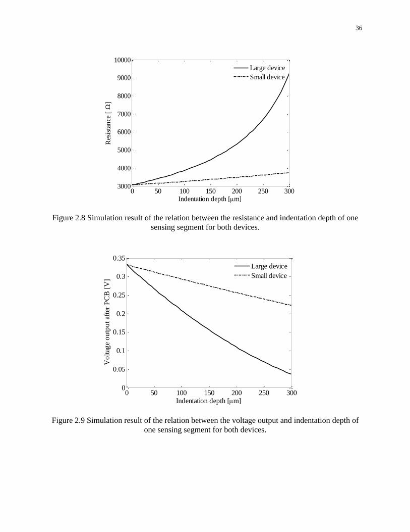
36
Figure 2.8 Simulation result of the relation between the resistance and indentation depth of one
sensing segment for both devices.
Figure 2.9 Simulation result of the relation between the voltage output and indentation depth of
one sensing segment for both devices.
0 50 100 150 200 250 3003000
4000
5000
6000
7000
8000
9000
10000
Indentation depth [m]
Res
ista
nce
[
]
Large device
Small device
0 50 100 150 200 250 3000
0.05
0.1
0.15
0.2
0.25
0.3
0.35
Indentation depth [m]
Vo
ltag
e o
utp
ut
afte
r P
CB
[V
]
Large device
Small device
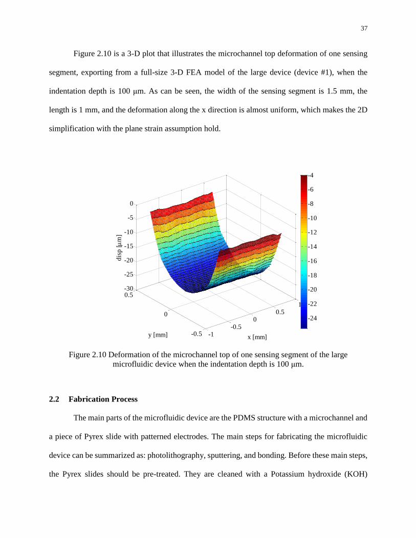
37
Figure 2.10 is a 3-D plot that illustrates the microchannel top deformation of one sensing
segment, exporting from a full-size 3-D FEA model of the large device (device #1), when the
indentation depth is 100 μm. As can be seen, the width of the sensing segment is 1.5 mm, the
length is 1 mm, and the deformation along the x direction is almost uniform, which makes the 2D
simplification with the plane strain assumption hold.
Figure 2.10 Deformation of the microchannel top of one sensing segment of the large
microfluidic device when the indentation depth is 100 μm.
2.2 Fabrication Process
The main parts of the microfluidic device are the PDMS structure with a microchannel and
a piece of Pyrex slide with patterned electrodes. The main steps for fabricating the microfluidic
device can be summarized as: photolithography, sputtering, and bonding. Before these main steps,
the Pyrex slides should be pre-treated. They are cleaned with a Potassium hydroxide (KOH)
-1-0.5
00.5
1
-0.5
0
0.5-30
-25
-20
-15
-10
-5
0
x [mm]y [mm]
dis
p [
m]
-24
-22
-20
-18
-16
-14
-12
-10
-8
-6
-4
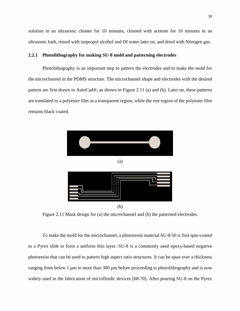
38
solution in an ultrasonic cleaner for 10 minutes, cleaned with acetone for 10 minutes in an
ultrasonic bath, rinsed with isopropyl alcohol and DI water later on, and dried with Nitrogen gas.
2.2.1 Photolithography for making SU-8 mold and patterning electrodes
Photolithography is an important step to pattern the electrodes and to make the mold for
the microchannel in the PDMS structure. The microchannel shape and electrodes with the desired
pattern are first drawn in AutoCad®, as shown in Figure 2.11 (a) and (b). Later on, these patterns
are translated to a polyester film as a transparent region, while the rest region of the polyester film
remains black coated.
(a)
(b)
Figure 2.11 Mask design for (a) the microchannel and (b) the patterned electrodes.
To make the mold for the microchannel, a photoresist material SU-8 50 is first spin-coated
to a Pyrex slide to form a uniform thin layer. SU-8 is a commonly used epoxy-based negative
photoresist that can be used to pattern high aspect ratio structures. It can be spun over a thickness
ranging from below 1 µm to more than 300 µm before proceeding to photolithography and is now
widely used in the fabrication of microfluidic devices [68-70]. After pouring SU-8 on the Pyrex
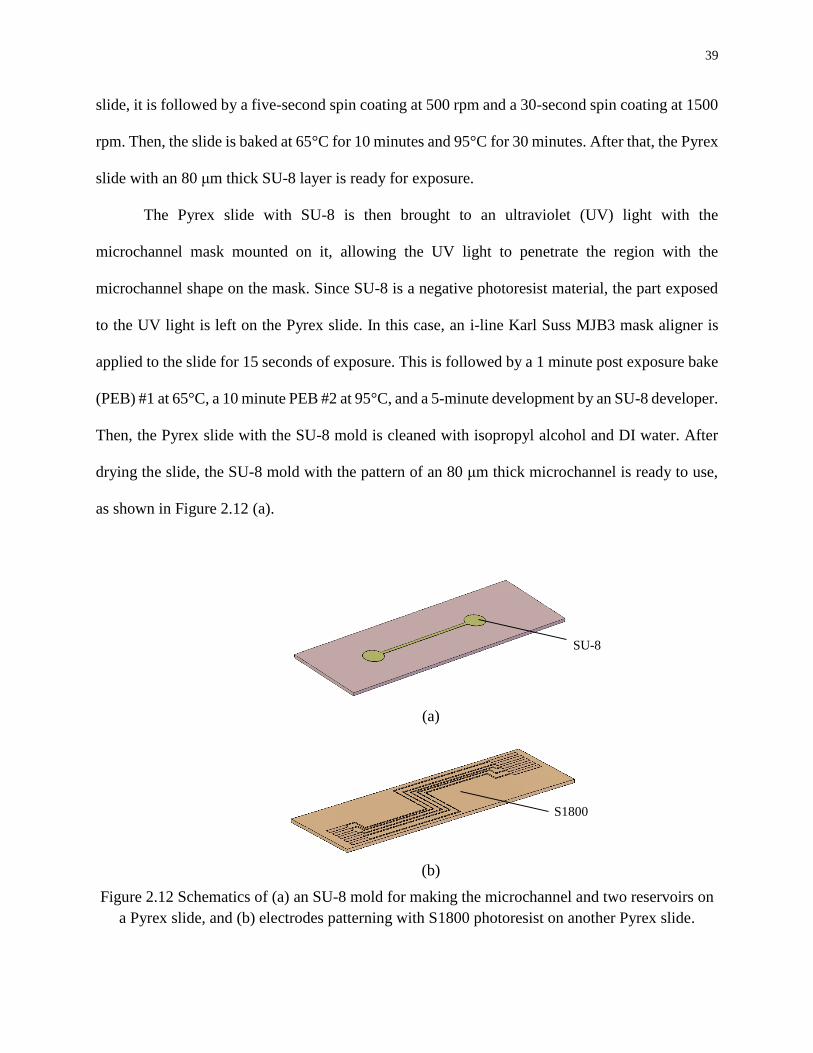
39
slide, it is followed by a five-second spin coating at 500 rpm and a 30-second spin coating at 1500
rpm. Then, the slide is baked at 65°C for 10 minutes and 95°C for 30 minutes. After that, the Pyrex
slide with an 80 μm thick SU-8 layer is ready for exposure.
The Pyrex slide with SU-8 is then brought to an ultraviolet (UV) light with the
microchannel mask mounted on it, allowing the UV light to penetrate the region with the
microchannel shape on the mask. Since SU-8 is a negative photoresist material, the part exposed
to the UV light is left on the Pyrex slide. In this case, an i-line Karl Suss MJB3 mask aligner is
applied to the slide for 15 seconds of exposure. This is followed by a 1 minute post exposure bake
(PEB) #1 at 65°C, a 10 minute PEB #2 at 95°C, and a 5-minute development by an SU-8 developer.
Then, the Pyrex slide with the SU-8 mold is cleaned with isopropyl alcohol and DI water. After
drying the slide, the SU-8 mold with the pattern of an 80 μm thick microchannel is ready to use,
as shown in Figure 2.12 (a).
(a)
(b)
Figure 2.12 Schematics of (a) an SU-8 mold for making the microchannel and two reservoirs on
a Pyrex slide, and (b) electrodes patterning with S1800 photoresist on another Pyrex slide.
SU-8
S1800
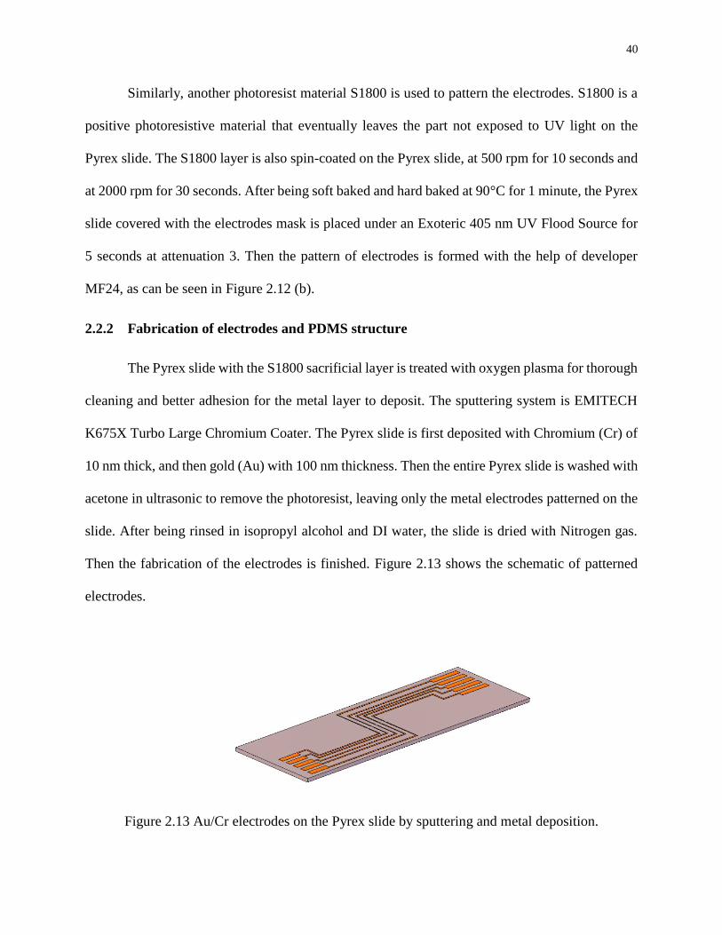
40
Similarly, another photoresist material S1800 is used to pattern the electrodes. S1800 is a
positive photoresistive material that eventually leaves the part not exposed to UV light on the
Pyrex slide. The S1800 layer is also spin-coated on the Pyrex slide, at 500 rpm for 10 seconds and
at 2000 rpm for 30 seconds. After being soft baked and hard baked at 90°C for 1 minute, the Pyrex
slide covered with the electrodes mask is placed under an Exoteric 405 nm UV Flood Source for
5 seconds at attenuation 3. Then the pattern of electrodes is formed with the help of developer
MF24, as can be seen in Figure 2.12 (b).
2.2.2 Fabrication of electrodes and PDMS structure
The Pyrex slide with the S1800 sacrificial layer is treated with oxygen plasma for thorough
cleaning and better adhesion for the metal layer to deposit. The sputtering system is EMITECH
K675X Turbo Large Chromium Coater. The Pyrex slide is first deposited with Chromium (Cr) of
10 nm thick, and then gold (Au) with 100 nm thickness. Then the entire Pyrex slide is washed with
acetone in ultrasonic to remove the photoresist, leaving only the metal electrodes patterned on the
slide. After being rinsed in isopropyl alcohol and DI water, the slide is dried with Nitrogen gas.
Then the fabrication of the electrodes is finished. Figure 2.13 shows the schematic of patterned
electrodes.
Figure 2.13 Au/Cr electrodes on the Pyrex slide by sputtering and metal deposition.
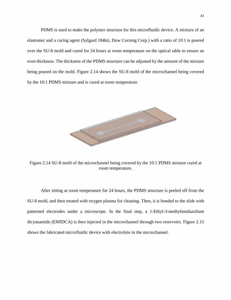
41
PDMS is used to make the polymer structure for this microfluidic device. A mixture of an
elastomer and a curing agent (Sylgard 184kit, Dow Corning Corp.) with a ratio of 10:1 is poured
over the SU-8 mold and cured for 24 hours at room temperature on the optical table to ensure an
even thickness. The thickness of the PDMS structure can be adjusted by the amount of the mixture
being poured on the mold. Figure 2.14 shows the SU-8 mold of the microchannel being covered
by the 10:1 PDMS mixture and is cured at room temperature.
Figure 2.14 SU-8 mold of the microchannel being covered by the 10:1 PDMS mixture cured at
room temperature.
After sitting at room temperature for 24 hours, the PDMS structure is peeled off from the
SU-8 mold, and then treated with oxygen plasma for cleaning. Then, it is bonded to the slide with
patterned electrodes under a microscope. In the final step, a 1-Ethyl-3-methylimidazolium
dicyanamide (EMIDCA) is then injected in the microchannel through two reservoirs. Figure 2.15
shows the fabricated microfluidic device with electrolyte in the microchannel.
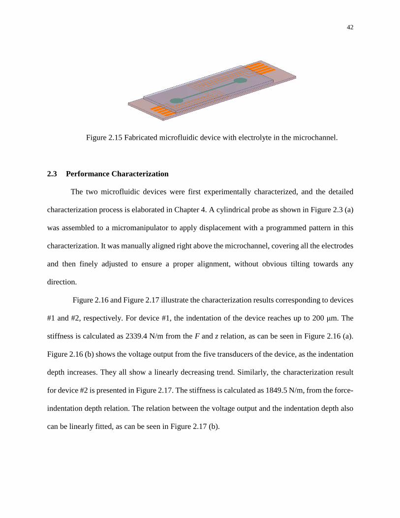
42
Figure 2.15 Fabricated microfluidic device with electrolyte in the microchannel.
2.3 Performance Characterization
The two microfluidic devices were first experimentally characterized, and the detailed
characterization process is elaborated in Chapter 4. A cylindrical probe as shown in Figure 2.3 (a)
was assembled to a micromanipulator to apply displacement with a programmed pattern in this
characterization. It was manually aligned right above the microchannel, covering all the electrodes
and then finely adjusted to ensure a proper alignment, without obvious tilting towards any
direction.
Figure 2.16 and Figure 2.17 illustrate the characterization results corresponding to devices
#1 and #2, respectively. For device #1, the indentation of the device reaches up to 200 μm. The
stiffness is calculated as 2339.4 N/m from the F and z relation, as can be seen in Figure 2.16 (a).
Figure 2.16 (b) shows the voltage output from the five transducers of the device, as the indentation
depth increases. They all show a linearly decreasing trend. Similarly, the characterization result
for device #2 is presented in Figure 2.17. The stiffness is calculated as 1849.5 N/m, from the force-
indentation depth relation. The relation between the voltage output and the indentation depth also
can be linearly fitted, as can be seen in Figure 2.17 (b).
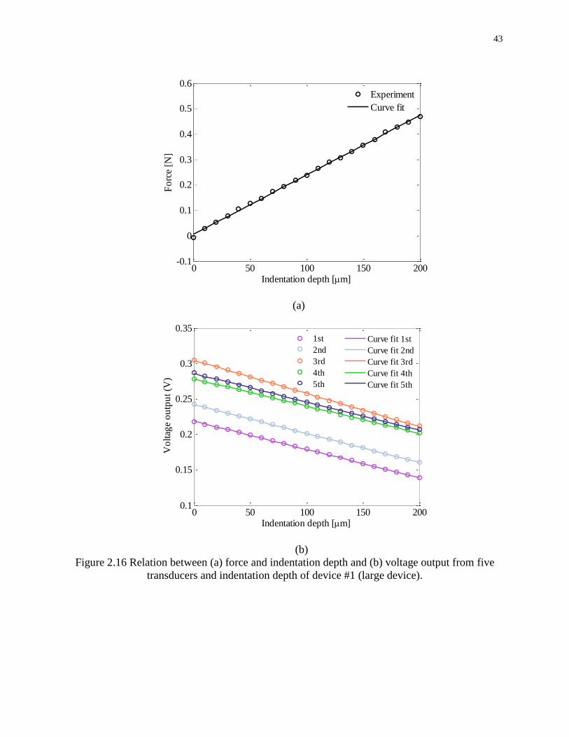
43
(a)
(b)
Figure 2.16 Relation between (a) force and indentation depth and (b) voltage output from five
transducers and indentation depth of device #1 (large device).
0 50 100 150 200-0.1
0
0.1
0.2
0.3
0.4
0.5
0.6
Indentation depth [m]
Fo
rce
[N]
Experiment
Curve fit
0 50 100 150 2000.1
0.15
0.2
0.25
0.3
0.35
Indentation depth [m]
Vo
ltag
e o
utp
ut
(V)
1st
2nd
3rd
4th
5th
Curve fit 1st
Curve fit 2nd
Curve fit 3rd
Curve fit 4th
Curve fit 5th
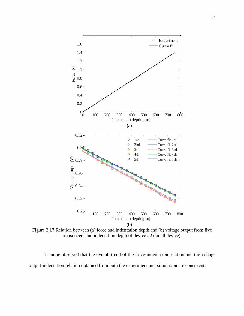
44
(a)
(b)
Figure 2.17 Relation between (a) force and indentation depth and (b) voltage output from five
transducers and indentation depth of device #2 (small device).
It can be observed that the overall trend of the force-indentation relation and the voltage
output-indentation relation obtained from both the experiment and simulation are consistent.
0 100 200 300 400 500 600 700 8000
0.2
0.4
0.6
0.8
1
1.2
1.4
1.6
Indentation depth [m]
Fo
rce
[N]
Experiment
Curve fit
0 100 200 300 400 500 600 700 8000.2
0.22
0.24
0.26
0.28
0.3
0.32
Indentation depth [m]
Vo
ltag
e o
utp
ut
(V)
1st
2nd
3rd
4th
5th
Curve fit 1st
Curve fit 2nd
Curve fit 3rd
Curve fit 4th
Curve fit 5th
45
However, in the experimental characterization, the voltage change is smaller than it is in the result
obtained by the numerical simulation.
The reasons for the discrepancy can be summarized as follows:
1) The actual dimensions of the devices vary a little from the nominal dimensions,
especially for the microchannel. The microchannel height has the smallest dimension among the
key design parameters. It plays an important role in the voltage output and is difficult to be
accurately measured. The initial resistance of one sensing segment for both devices is supposed to
be 3067 Ω theoretically, corresponding to a microchannel height of 80 μm. The theoretical voltage
output from the circuit is supposed to be 0.332 V, corresponding to a feedback resistance of 25 kΩ
and 200 mV peak-to-peak voltage input. However, from Figure 2.16 (b) and Figure 2.17 (b), it is
noticed that the initial voltage output from the five transducers of both devices is less than 0.332
V, which could be caused by fabrication defects. For instance, a less than 80 μm microchannel
height for both devices can cause such situations. The voltage output of the five transducers also
varies, which can be attributed to the fabrication variations, especially in the microchannel height
at the transducer locations. The effect of the microchannel height on the resistance and voltage
output of each sensing segment is discussed in Section 2.4.
2) Mechanical and Electrical Crosstalk. In the previous simulation, it is assumed that the
effective width of each sensing segment equals the transducer spacing, and no mechanical or
electrical crosstalk exists between the neighboring sensing segments. However, the real interaction
between the neighboring sensing segments is more complicated. From the electrical side, the
conductive portion is a liquid that flows between the sensing segments, making the interaction
between the neighboring transducers inevitable. From the mechanical side, all sensing segments
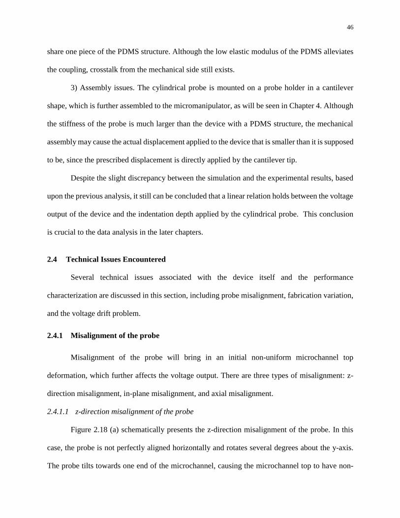
46
share one piece of the PDMS structure. Although the low elastic modulus of the PDMS alleviates
the coupling, crosstalk from the mechanical side still exists.
3) Assembly issues. The cylindrical probe is mounted on a probe holder in a cantilever
shape, which is further assembled to the micromanipulator, as will be seen in Chapter 4. Although
the stiffness of the probe is much larger than the device with a PDMS structure, the mechanical
assembly may cause the actual displacement applied to the device that is smaller than it is supposed
to be, since the prescribed displacement is directly applied by the cantilever tip.
Despite the slight discrepancy between the simulation and the experimental results, based
upon the previous analysis, it still can be concluded that a linear relation holds between the voltage
output of the device and the indentation depth applied by the cylindrical probe. This conclusion
is crucial to the data analysis in the later chapters.
2.4 Technical Issues Encountered
Several technical issues associated with the device itself and the performance
characterization are discussed in this section, including probe misalignment, fabrication variation,
and the voltage drift problem.
2.4.1 Misalignment of the probe
Misalignment of the probe will bring in an initial non-uniform microchannel top
deformation, which further affects the voltage output. There are three types of misalignment: z-
direction misalignment, in-plane misalignment, and axial misalignment.
2.4.1.1 z-direction misalignment of the probe
Figure 2.18 (a) schematically presents the z-direction misalignment of the probe. In this
case, the probe is not perfectly aligned horizontally and rotates several degrees about the y-axis.
The probe tilts towards one end of the microchannel, causing the microchannel top to have non-
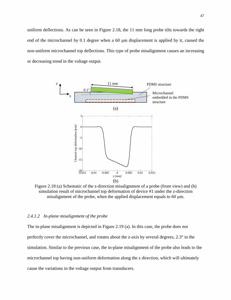
47
uniform deflections. As can be seen in Figure 2.18, the 11 mm long probe tilts towards the right
end of the microchannel by 0.1 degree when a 60 μm displacement is applied by it, caused the
non-uniform microchannel top deflections. This type of probe misalignment causes an increasing
or decreasing trend in the voltage output.
(a)
(b)
Figure 2.18 (a) Schematic of the z-direction misalignment of a probe (front view) and (b)
simulation result of microchannel top deformation of device #1 under the z-direction
misalignment of the probe, when the applied displacement equals to 60 μm.
2.4.1.2 In-plane misalignment of the probe
The in-plane misalignment is depicted in Figure 2.19 (a). In this case, the probe does not
perfectly cover the microchannel, and rotates about the z-axis by several degrees, 2.3° in the
simulation. Similar to the previous case, the in-plane misalignment of the probe also leads to the
microchannel top having non-uniform deformation along the z direction, which will ultimately
cause the variations in the voltage output from transducers.
-0.015 -0.01 -0.005 0 0.005 0.01 0.015-20
-15
-10
-5
0
5
x [mm]
Ch
ann
el t
op
def
orm
atio
n [
m
]
z
x
0.1° 11 mm PDMS structure
Microchannel
embedded in the PDMS
structure
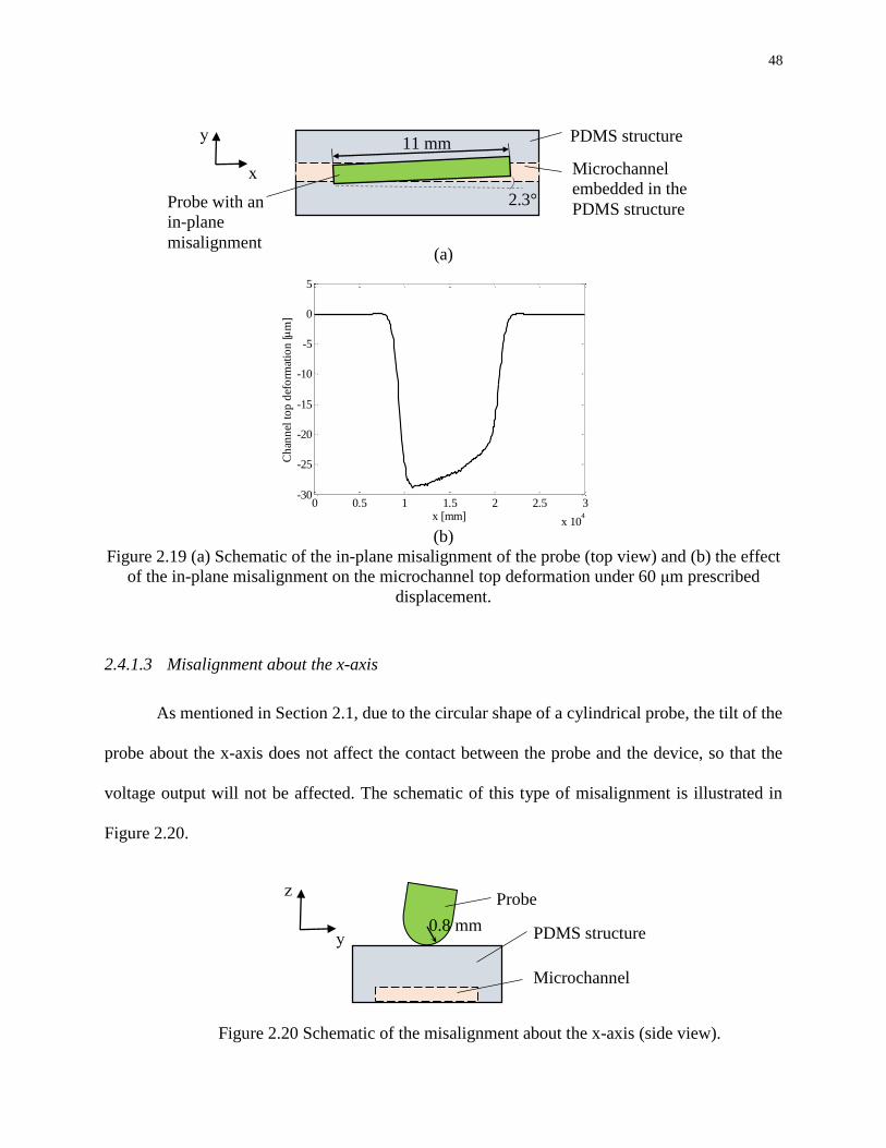
48
(a)
(b)
Figure 2.19 (a) Schematic of the in-plane misalignment of the probe (top view) and (b) the effect
of the in-plane misalignment on the microchannel top deformation under 60 μm prescribed
displacement.
2.4.1.3 Misalignment about the x-axis
As mentioned in Section 2.1, due to the circular shape of a cylindrical probe, the tilt of the
probe about the x-axis does not affect the contact between the probe and the device, so that the
voltage output will not be affected. The schematic of this type of misalignment is illustrated in
Figure 2.20.
Figure 2.20 Schematic of the misalignment about the x-axis (side view).
0 0.5 1 1.5 2 2.5 3
x 104
-30
-25
-20
-15
-10
-5
0
5
x [mm]
Ch
ann
el t
op
def
orm
atio
n [
m
]
z
y
2.3°
PDMS structure
Microchannel
embedded in the
PDMS structure Probe with an
in-plane
misalignment
y
x
11 mm
0.8 mm
Microchannel
PDMS structure
Probe
2.3°

49
2.4.2 Fabrication variations
Fabrication variations are other issues that affect the device performance. Microchannel
height is one of the variations that could significantly affect the voltage output from the device,
since it has the smallest dimension among all the key design parameters. The microchannel height
of the device is determined by the thickness of the SU-8 mold used for fabricating the
microchannel, as mentioned in Section 2.2.1. It is inevitable that the thickness of the mold has
some variations. A simulation of the sensor with a varying microchannel height is carried out. The
microchannel height varies from 50 μm to 80 μm, from the left to the right, as shown in Figure
2.21. As can be seen in Table 2.3, the initial resistance decreases from transducer 1 to transducer
5. When a 60 μm prescribed displacement is applied, the corresponding resistance and voltage
output values of each sensing segment are also listed in Table 2.3.
Figure 2.21 Schematic of a device with variations in microchannel height (front view).
Table 2.3 Resistance and voltage output of a device with varying microchannel height at the
locations of the transducers.
Transducer 1 2 3 4 5
Initial resistance (Ω) 3982 3888 3798 3713 3631
60 μm resistance (Ω) 3996 3901 3811 3726 3642
Initial voltage (V) 0.1971 0.2067 0.2166 0.2267 0.2370
60 μm voltage (V) 0.1957 0.2054 0.2152 0.2251 0.2356
ΔV (V) 0.0014 0.0013 0.0014 0.0016 0.0014
50 μm 80 μm
z
x
Probe PDMS structure
Microchannel
embedded in the PDMS
structure
50
2.4.3 Voltage drift
So far, NaCl, KCl solutions and a 1-ethyl-3-methylimidazolium dicyanamide have been
used as the electrolyte for the microfluidic device. It is proved in a previous publication that a 1-
ethyl-3-methylimidazolium dicyanamide has very low volatility, compared with NaCl, KCl
solutions, and is desirable for being a stable conductive liquid [62]. Despite the excellent electrical
stability, a voltage drift is still detected from the experiment.
Figures 2.22 and 2.23 exhibit the voltage drift of the device during one week and during
one dynamic measurement which lasts for one to two hours. To investigate if the voltage output
would be stable after the heat equilibrium is established, the device is connected to the circuit and
left on for 48 hours. The test result is shown in Appendix B. Overall, the voltage output shows a
decreasing trend with time. It means if the voltage drift is caused by the heat dissipation, 48 hours
are not enough to allow the device to reach its heat equilibrium, which is not practical in the real
operation. Other groups have also reported on the voltage drift phenomenon during the operation
of a microfluidic device. Chossat et al. [71] attributed the drift to the evaporation of the water in
the electrolyte, eutectic gallium indium (eGaIn), due to an imperfect bonding, sealing, or the
permeability of the material. Collins et al. [72] also mentioned the voltage drift in their work which
employed sodium hydroxide (NaOH) solution as the electrolyte. Its ability of absorbing CO2 in the
air and form carbonic acid is accounting for the voltage drift. Muth et al. [73] used carbon
conductive grease as the conductive liquid in their 3D printed devices, but the voltage drift problem
still exists. Scott et al. [74] mentioned Ag/AgCl electrodes are electrochemically stable, which can
avoid the artifacts from voltage drift caused by polarizable metal electrodes. To the best knowledge
of the author, voltage drift issues in microfluidic devices have not been thoroughly studied or
solved yet. This issue is reported in this section for completeness.
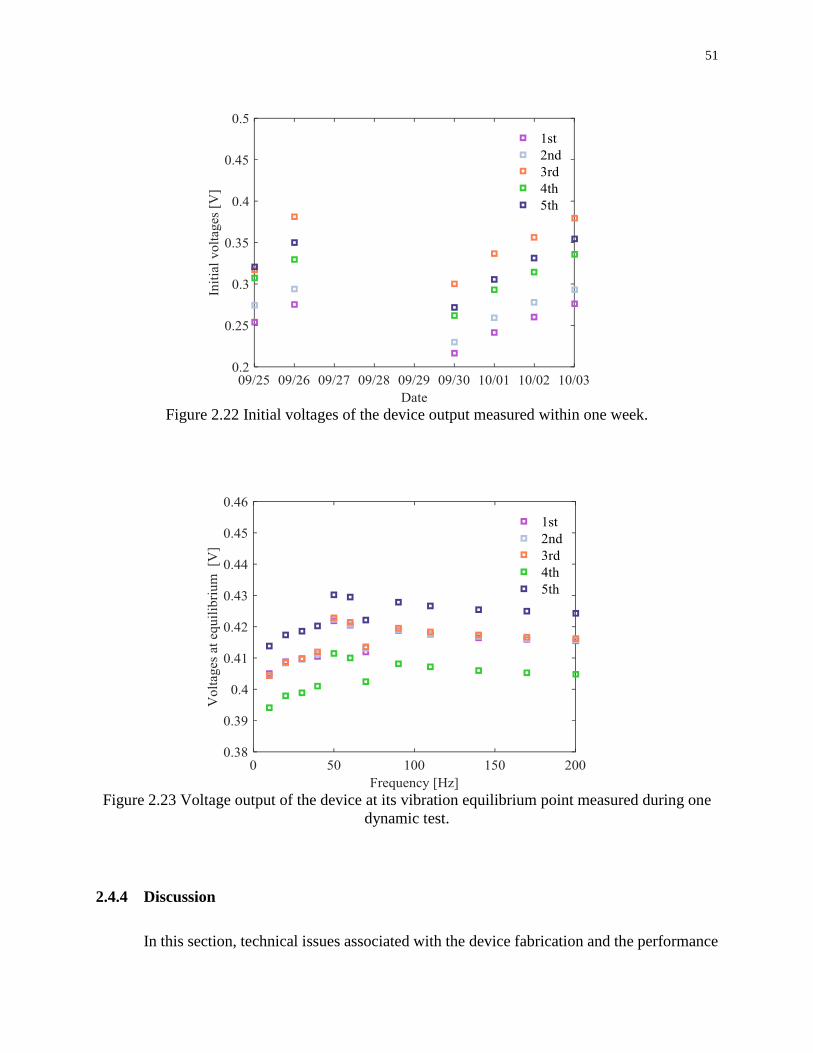
51
Figure 2.22 Initial voltages of the device output measured within one week.
Figure 2.23 Voltage output of the device at its vibration equilibrium point measured during one
dynamic test.
2.4.4 Discussion
In this section, technical issues associated with the device fabrication and the performance
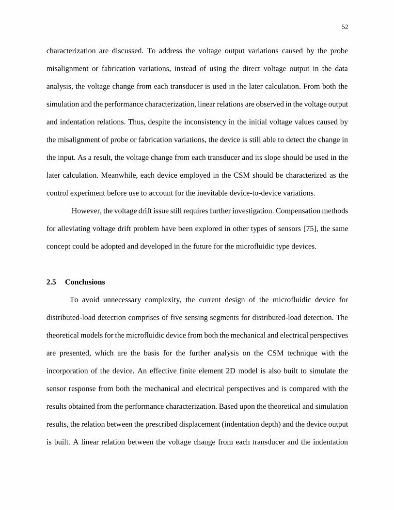
52
characterization are discussed. To address the voltage output variations caused by the probe
misalignment or fabrication variations, instead of using the direct voltage output in the data
analysis, the voltage change from each transducer is used in the later calculation. From both the
simulation and the performance characterization, linear relations are observed in the voltage output
and indentation relations. Thus, despite the inconsistency in the initial voltage values caused by
the misalignment of probe or fabrication variations, the device is still able to detect the change in
the input. As a result, the voltage change from each transducer and its slope should be used in the
later calculation. Meanwhile, each device employed in the CSM should be characterized as the
control experiment before use to account for the inevitable device-to-device variations.
However, the voltage drift issue still requires further investigation. Compensation methods
for alleviating voltage drift problem have been explored in other types of sensors [75], the same
concept could be adopted and developed in the future for the microfluidic type devices.
2.5 Conclusions
To avoid unnecessary complexity, the current design of the microfluidic device for
distributed-load detection comprises of five sensing segments for distributed-load detection. The
theoretical models for the microfluidic device from both the mechanical and electrical perspectives
are presented, which are the basis for the further analysis on the CSM technique with the
incorporation of the device. An effective finite element 2D model is also built to simulate the
sensor response from both the mechanical and electrical perspectives and is compared with the
results obtained from the performance characterization. Based upon the theoretical and simulation
results, the relation between the prescribed displacement (indentation depth) and the device output
is built. A linear relation between the voltage change from each transducer and the indentation

53
depth will be used in the data analysis for extracting the viscoelastic properties of testing materials
in later chapters. The fabrication process for the polymer-based microfluidic device shows its
simplicity and low cost. Several technical issues associated with the device itself and the testing
method are also discussed to account for the potential errors the output data from the device could
carry.
The performance of the device is robust, however from the design and fabrication
perspectives, there are several aspects worth being improved in a future design. For example, the
mechanical and electrical interference between the sensing segments should be considered and
alleviated in a future design. Other more compliant elastomers can be used to build the mechanical
structure of the microfluidic device for larger deformation or stretching. Other conductive liquids
could be employed as the electrolyte to alleviate the voltage drift problem existing in the current
sensor. Meanwhile, other fabrication techniques, such as 3D printing, could also be considered in
the future.
Overall, in this chapter, the polymer-based microfluidic device employed for the CSM in
later chapters is presented. The working principle, fabrication process, performance
characterization, and technical issues encountered in the experimental characterization are
thoroughly discussed.

54
CHAPTER 3
CONCURRENT SPATIAL MAPPING OF THE ELASTIC MODULUS OF SOFT
MATERIALS: THEORY
This chapter explores the theory and rationale of conducting the CSM technique to obtain
the spatially-varying elastic modulus of heterogeneous soft materials via the microfluidic device.
This chapter first describes the related knowledge in the field of contact mechanics associated with
the CSM technique. Then the rationale of conducting the CSM is explained in detail. Next, the
capability of detecting the heterogeneity in a sample through the microfluidic device is studied
through the FEA method. The effect of the heterogeneity parameters on the device output is also
explored.
3.1 Contact Mechanics
In a CSM of the elastic modulus, a cylindrical probe is used to press a material sample
against the device to obtain the force and indentation depth relation at the locations of the
transducers. Thus, it is essential to obtain an accurate model to relate the elastic modulus to the
measurable force and indentation depth applied to the material sample.
Figure 3.1 schematically shows a cylinder probe is in contact with a flat sheet with infinite
thickness and indents the flat sheet with a depth of δ. Puttock and Thwaite [2] derived the relation
between the reaction force and the indentation depth of a cylinder in contact with a flat sheet with
infinite thickness. As can be seen in Equation 3.1, the indentation depth δ is related to the reaction
force F and the material properties.
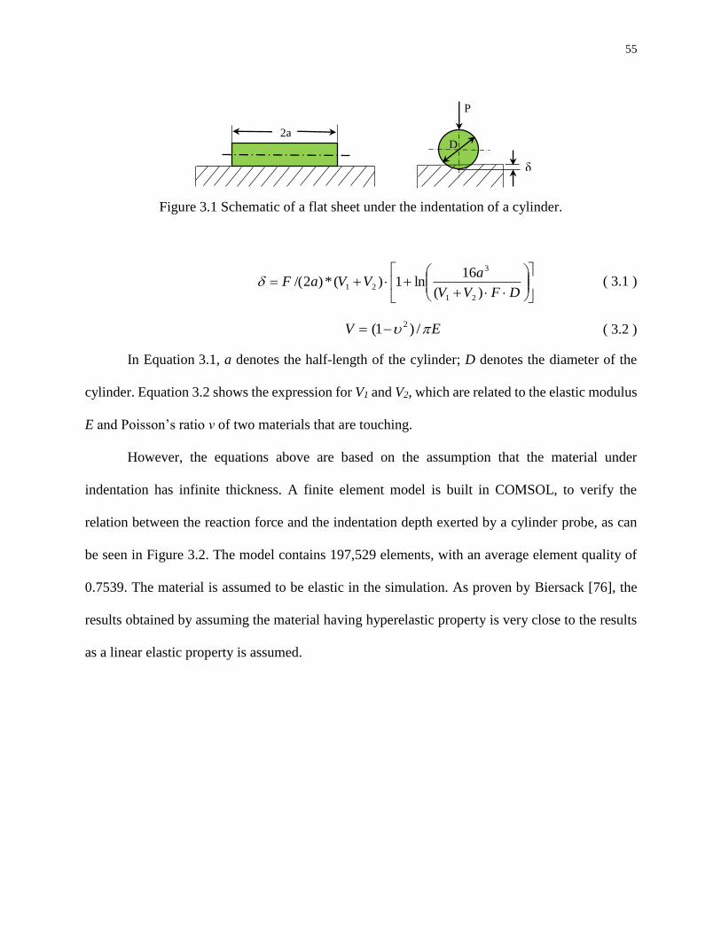
55
Figure 3.1 Schematic of a flat sheet under the indentation of a cylinder.
DFVV
aVVaF
)(
16ln1)(*)2/(
21
3
21 ( 3.1 )
EV /)1( 2 ( 3.2 )
In Equation 3.1, a denotes the half-length of the cylinder; D denotes the diameter of the
cylinder. Equation 3.2 shows the expression for V1 and V2, which are related to the elastic modulus
E and Poisson’s ratio ν of two materials that are touching.
However, the equations above are based on the assumption that the material under
indentation has infinite thickness. A finite element model is built in COMSOL, to verify the
relation between the reaction force and the indentation depth exerted by a cylinder probe, as can
be seen in Figure 3.2. The model contains 197,529 elements, with an average element quality of
0.7539. The material is assumed to be elastic in the simulation. As proven by Biersack [76], the
results obtained by assuming the material having hyperelastic property is very close to the results
as a linear elastic property is assumed.
2a
P
δ
D
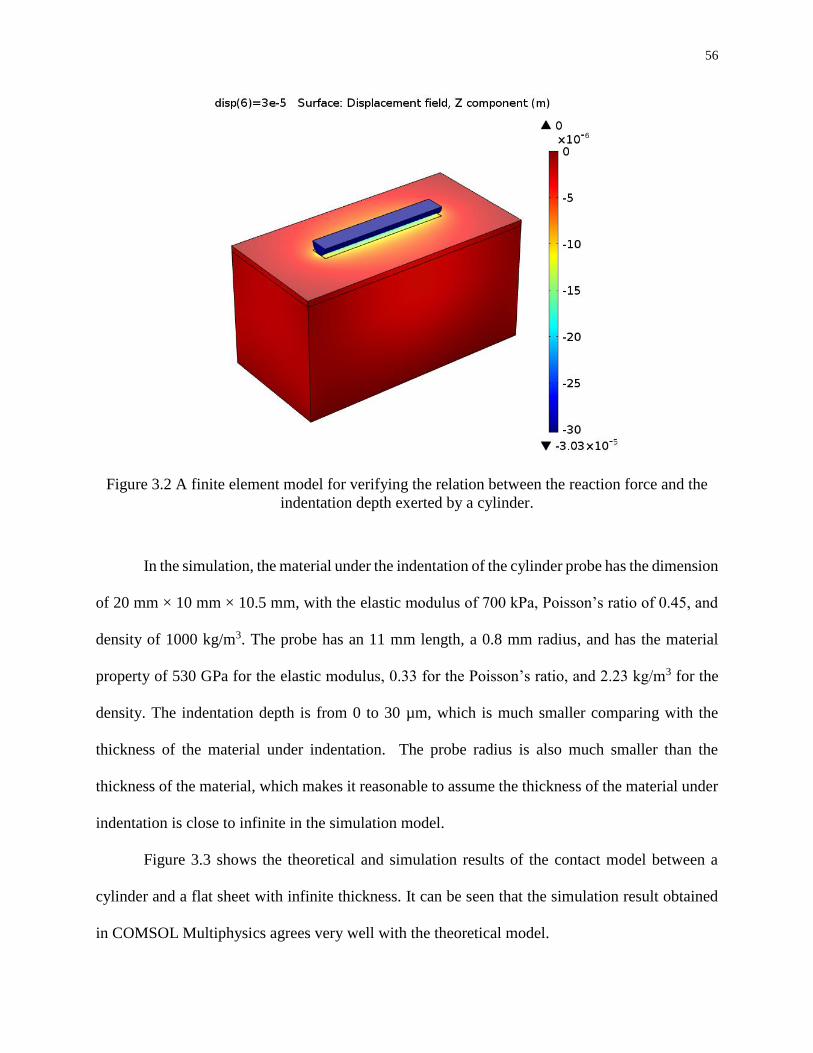
56
Figure 3.2 A finite element model for verifying the relation between the reaction force and the
indentation depth exerted by a cylinder.
In the simulation, the material under the indentation of the cylinder probe has the dimension
of 20 mm × 10 mm × 10.5 mm, with the elastic modulus of 700 kPa, Poisson’s ratio of 0.45, and
density of 1000 kg/m3. The probe has an 11 mm length, a 0.8 mm radius, and has the material
property of 530 GPa for the elastic modulus, 0.33 for the Poisson’s ratio, and 2.23 kg/m3 for the
density. The indentation depth is from 0 to 30 µm, which is much smaller comparing with the
thickness of the material under indentation. The probe radius is also much smaller than the
thickness of the material, which makes it reasonable to assume the thickness of the material under
indentation is close to infinite in the simulation model.
Figure 3.3 shows the theoretical and simulation results of the contact model between a
cylinder and a flat sheet with infinite thickness. It can be seen that the simulation result obtained
in COMSOL Multiphysics agrees very well with the theoretical model.

57
Figure 3.3 Theoretical and FEA simulation results of the contact model of a cylinder and a flat
sheet with infinite thickness.
However, the thickness of a sample will start to affect the accuracy of the results obtained
by Equations 3.1 and 3.2, when the thickness of the sample gets close to the diameter of the probe
or the indentation depth. It is necessary to bring in a correction factor to Equation 3.1 in order to
achieve a more accurate elastic modulus that relates the force and indentation depth. For a spherical
indenter that is commonly used in AFM or a nanoindenter, modifications were made to the widely
used Hertz model to account for the effect of the finite thickness of a sample by Dimitriadis [25].
However, to author’s knowledge, there is sparse research that highlights the derivation of the
analytical form of a cylinder in contact with a flat sheet with finite thickness, which only applies
to special cases [77-79]. There is no analytical solution in a general case to account for the effect
of the thickness of a flat sheet on the overall force and indentation relation under the press of a
cylinder probe.
0 5 10 15 20 25 30 35 400
0.02
0.04
0.06
0.08
0.1
Indentation depth [m]
Fo
rce
(N)
Simulation
Theory
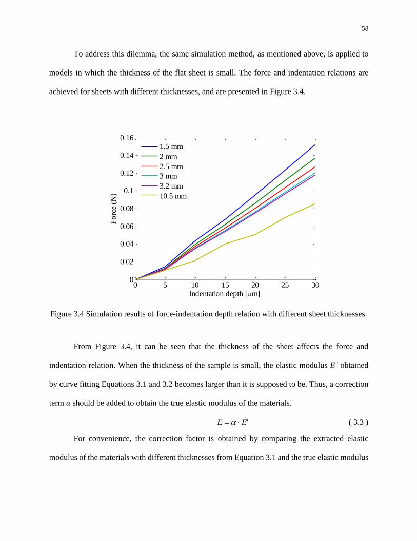
58
To address this dilemma, the same simulation method, as mentioned above, is applied to
models in which the thickness of the flat sheet is small. The force and indentation relations are
achieved for sheets with different thicknesses, and are presented in Figure 3.4.
Figure 3.4 Simulation results of force-indentation depth relation with different sheet thicknesses.
From Figure 3.4, it can be seen that the thickness of the sheet affects the force and
indentation relation. When the thickness of the sample is small, the elastic modulus E’ obtained
by curve fitting Equations 3.1 and 3.2 becomes larger than it is supposed to be. Thus, a correction
term α should be added to obtain the true elastic modulus of the materials.
EE ( 3.3 )
For convenience, the correction factor is obtained by comparing the extracted elastic
modulus of the materials with different thicknesses from Equation 3.1 and the true elastic modulus
0 5 10 15 20 25 300
0.02
0.04
0.06
0.08
0.1
0.12
0.14
0.16
Indentation depth [m]
Fo
rce
(N)
1.5 mm
2 mm
2.5 mm
3 mm
3.2 mm
10.5 mm
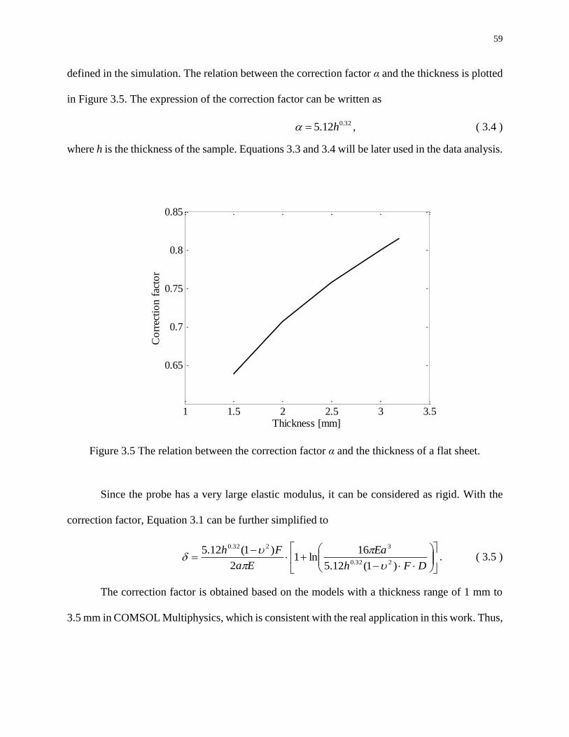
59
defined in the simulation. The relation between the correction factor α and the thickness is plotted
in Figure 3.5. The expression of the correction factor can be written as
32.012.5 h , ( 3.4 )
where h is the thickness of the sample. Equations 3.3 and 3.4 will be later used in the data analysis.
Figure 3.5 The relation between the correction factor α and the thickness of a flat sheet.
Since the probe has a very large elastic modulus, it can be considered as rigid. With the
correction factor, Equation 3.1 can be further simplified to
DFh
Ea
Ea
Fh
)1(12.5
16ln1
2
)1(12.5232.0
3232.0
. ( 3.5 )
The correction factor is obtained based on the models with a thickness range of 1 mm to
3.5 mm in COMSOL Multiphysics, which is consistent with the real application in this work. Thus,
1 1.5 2 2.5 3 3.5
0.65
0.7
0.75
0.8
0.85
Thickness [mm]
Co
rrec
tio
n f
acto
r
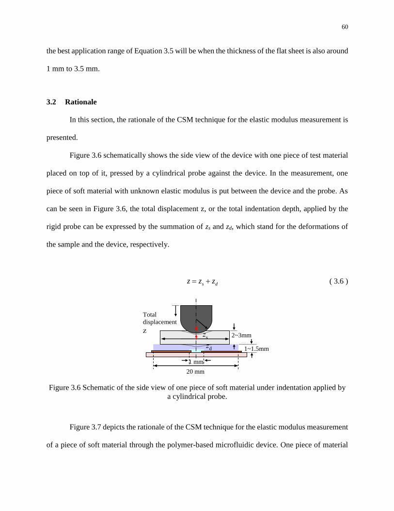
60
the best application range of Equation 3.5 will be when the thickness of the flat sheet is also around
1 mm to 3.5 mm.
3.2 Rationale
In this section, the rationale of the CSM technique for the elastic modulus measurement is
presented.
Figure 3.6 schematically shows the side view of the device with one piece of test material
placed on top of it, pressed by a cylindrical probe against the device. In the measurement, one
piece of soft material with unknown elastic modulus is put between the device and the probe. As
can be seen in Figure 3.6, the total displacement z, or the total indentation depth, applied by the
rigid probe can be expressed by the summation of zs and zd, which stand for the deformations of
the sample and the device, respectively.
ds zzz ( 3.6 )
Figure 3.6 Schematic of the side view of one piece of soft material under indentation applied by
a cylindrical probe.
Figure 3.7 depicts the rationale of the CSM technique for the elastic modulus measurement
of a piece of soft material through the polymer-based microfluidic device. One piece of material
1 mm
2~3mm
1~1.5mm
zs
zd
20 mm
Total
displacement
z
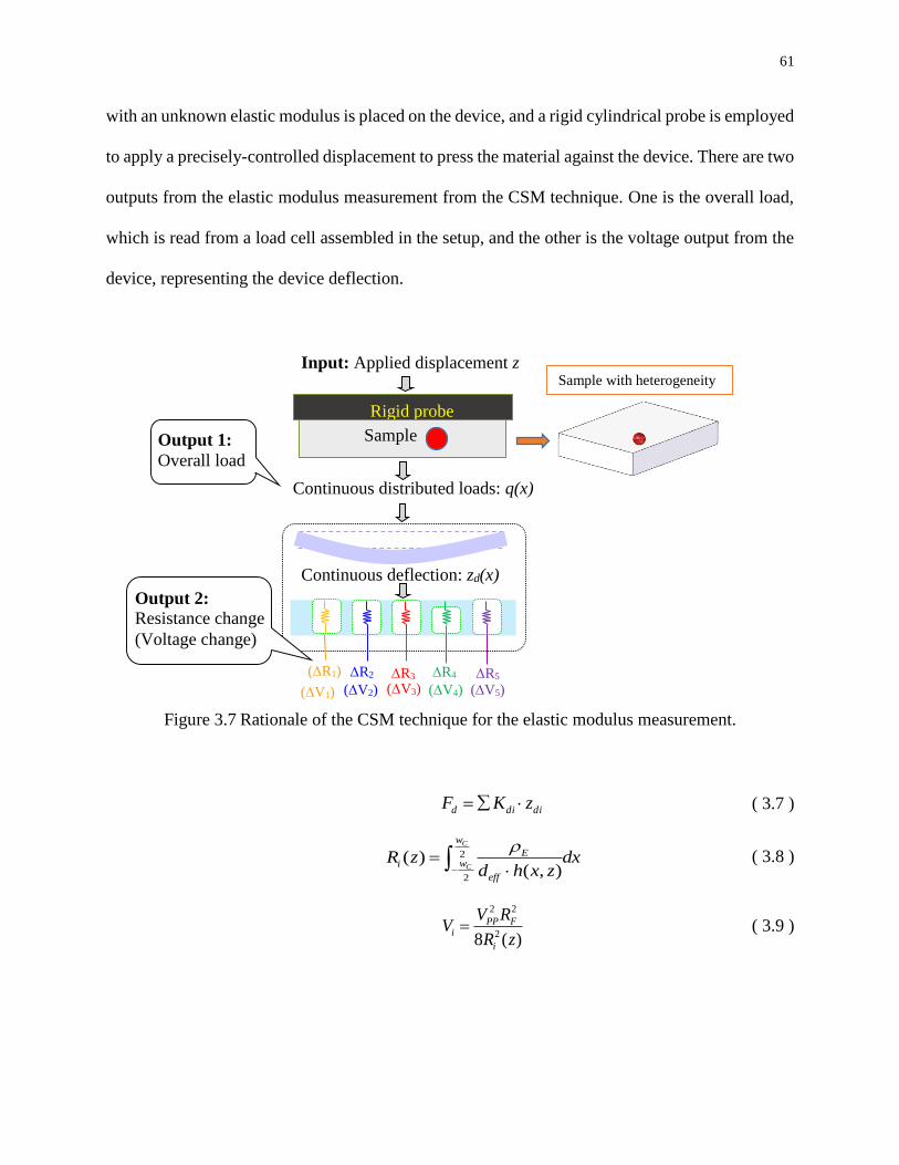
61
with an unknown elastic modulus is placed on the device, and a rigid cylindrical probe is employed
to apply a precisely-controlled displacement to press the material against the device. There are two
outputs from the elastic modulus measurement from the CSM technique. One is the overall load,
which is read from a load cell assembled in the setup, and the other is the voltage output from the
device, representing the device deflection.
Figure 3.7 Rationale of the CSM technique for the elastic modulus measurement.
didid zKF ( 3.7 )
2
2
( )( , )
C
C
w
Ewi
eff
R z dxd h x z
( 3.8 )
2 2
28 ( )
PP Fi
i
V RV
R z ( 3.9 )
(V1) (V2) (V3) (V4) (V5)
Rigid probe
Input: Applied displacement z
Continuous distributed loads: q(x)
Continuous deflection: zd(x)
Sample Output 1:
Overall load
(R1) R2 R3 R4 R5
Output 2: Resistance change
(Voltage change)
Sample with heterogeneity
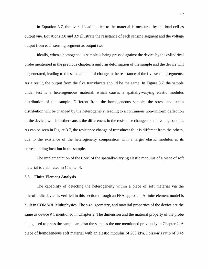
62
In Equation 3.7, the overall load applied to the material is measured by the load cell as
output one. Equations 3.8 and 3.9 illustrate the resistance of each sensing segment and the voltage
output from each sensing segment as output two.
Ideally, when a homogeneous sample is being pressed against the device by the cylindrical
probe mentioned in the previous chapter, a uniform deformation of the sample and the device will
be generated, leading to the same amount of change in the resistance of the five sensing segments.
As a result, the output from the five transducers should be the same. In Figure 3.7, the sample
under test is a heterogeneous material, which causes a spatially-varying elastic modulus
distribution of the sample. Different from the homogeneous sample, the stress and strain
distribution will be changed by the heterogeneity, leading to a continuous non-uniform deflection
of the device, which further causes the differences in the resistance change and the voltage output.
As can be seen in Figure 3.7, the resistance change of transducer four is different from the others,
due to the existence of the heterogeneity composition with a larger elastic modulus at its
corresponding location in the sample.
The implementation of the CSM of the spatially-varying elastic modulus of a piece of soft
material is elaborated in Chapter 4.
3.3 Finite Element Analysis
The capability of detecting the heterogeneity within a piece of soft material via the
microfluidic device is verified in this section through an FEA approach. A finite element model is
built in COMSOL Multiphysics. The size, geometry, and material properties of the device are the
same as device # 1 mentioned in Chapter 2. The dimension and the material property of the probe
being used to press the sample are also the same as the one mentioned previously in Chapter 2. A
piece of homogeneous soft material with an elastic modulus of 200 kPa, Poisson’s ratio of 0.45

63
and density of 1 kg/m3 is first built between the probe and the device. The in-plane dimension of
the piece of material is 15 mm×6 mm; the thickness is 2.5 mm. It is placed on top of the device,
covering the five transducers. A piece of heterogeneous soft material is modeled in the second
simulation. To simplify the model, a sphere-shaped geometry with a radius of 0.5 mm and a high
elastic modulus of 2 GPa is built in the model to mimic the heterogeneity inside a material. As can
be seen in Figure 3.8, the hard sphere is located above one of the transducers.
Figure 3.8 Simulation of a piece of heterogeneous material under the indentation applied
by a cylindrical probe on a microfluidic force sensor.
Figure 3.9 presents the simulation result of the microchannel top deformation when a piece
of homogeneous material is being pressed against the device. The microchannel is 30 mm in
length, and the probe is 11 mm long, which explains the majority of the deformation happens in
the central area of the microchannel top. The five transducers are 1.5 mm away from each other,
locating in the middle section of the microchannel, along the microchannel length. To be specific,
they are located at 12 mm, 13.5 mm, 15 mm, 16.5 mm and 18 mm, corresponding to the horizontal
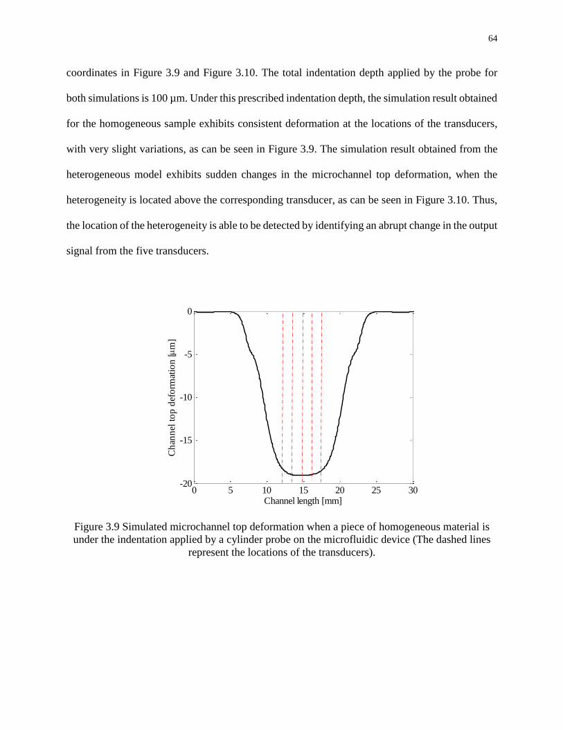
64
coordinates in Figure 3.9 and Figure 3.10. The total indentation depth applied by the probe for
both simulations is 100 µm. Under this prescribed indentation depth, the simulation result obtained
for the homogeneous sample exhibits consistent deformation at the locations of the transducers,
with very slight variations, as can be seen in Figure 3.9. The simulation result obtained from the
heterogeneous model exhibits sudden changes in the microchannel top deformation, when the
heterogeneity is located above the corresponding transducer, as can be seen in Figure 3.10. Thus,
the location of the heterogeneity is able to be detected by identifying an abrupt change in the output
signal from the five transducers.
Figure 3.9 Simulated microchannel top deformation when a piece of homogeneous material is
under the indentation applied by a cylinder probe on the microfluidic device (The dashed lines
represent the locations of the transducers).
0 5 10 15 20 25 30-20
-15
-10
-5
0
Channel length [mm]
Ch
ann
el t
op
def
orm
atio
n [
m
]

65
Figure 3.10 Simulated microchannel top deformation when a piece of heterogeneous material
under compression by a cylinder probe on the microfluidic force sensor. (The dashed lines
represent the locations of the transducers.)
Figure 3.11 Simulation of a piece of material sample with a hard sphere (r = 1.2 mm) embedded,
indented by a cylindrical probe on the microfluidic device.
0 5 10 15 20 25 30-25
-20
-15
-10
-5
0
Channel length [mm]
Ch
ann
el t
op
def
orm
atio
n [
m
]
Location 1
Location 2
Location 3
Location 4
Location 5
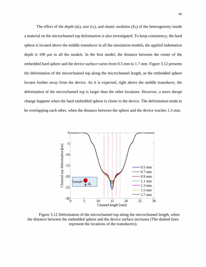
66
The effect of the depth (dh), size (rh), and elastic modulus (Eh) of the heterogeneity inside
a material on the microchannel top deformation is also investigated. To keep consistency, the hard
sphere is located above the middle transducer in all the simulation models, the applied indentation
depth is 100 μm in all the models. In the first model, the distance between the center of the
embedded hard sphere and the device surface varies from 0.5 mm to 1.7 mm. Figure 3.12 presents
the deformation of the microchannel top along the microchannel length, as the embedded sphere
locates further away from the device. As it is expected, right above the middle transducer, the
deformation of the microchannel top is larger than the other locations. However, a more abrupt
change happens when the hard embedded sphere is closer to the device. The deformation tends to
be overlapping each other, when the distance between the sphere and the device reaches 1.3 mm.
Figure 3.12 Deformation of the microchannel top along the microchannel length, when
the distance between the embedded sphere and the device surface increases (The dashed lines
represent the locations of the transducers).
0 5 10 15 20 25 30-30
-25
-20
-15
-10
-5
0
Channel length [mm]
Ch
ann
el t
op
def
orm
atio
n [
m]
0.5 mm
0.7 mm
0.9 mm
1.1 mm
1.3 mm
1.5 mm
1.7 mm
Sample dh
67
In the second simulation model, the radius of the embedded sphere varies from 0.2 mm to
1.2 mm with a 0.2 mm interval, while the center of the hard sphere is located right in the middle
of the sample. Figure 3.13 shows the deformation of the microchannel top along the microchannel
length, as the radius of the embedded sphere increases. As can be seen, the hard sphere is no longer
detectable, when the radius is below 0.4 mm. It can be concluded that the radius of the hard sphere
has a larger impact on the microchannel deformation, since an approximate 40 µm change occurs
at the microchannel top, when the sphere radius is as large as 1.2 mm.
Figure 3.13 Deformation of the microchannel top along the microchannel length, when the radius
of the embedded sphere increases (The dashed lines represent the locations of the transducers).
In the third model, the varying parameter is the elastic modulus of the sphere, which varies
from 500 kPa to 4.9 MPa. The sphere representing the heterogeneity has a radius of 0.5 mm, and
is located in the middle of the sample. The simulation result is presented in Figure 3.14. It is noticed
that although the deformation of the microchannel top increases with the elastic modulus of the
0 5 10 15 20 25 30-60
-50
-40
-30
-20
-10
0
Channel length [mm]
Ch
ann
el t
op
def
orm
atio
n [
m]
r=0.2 mm
r=0.4 mm
r=0.6 mm
r=0.8 mm
r=1.0 mm
r=1.2 mm
Sample rh
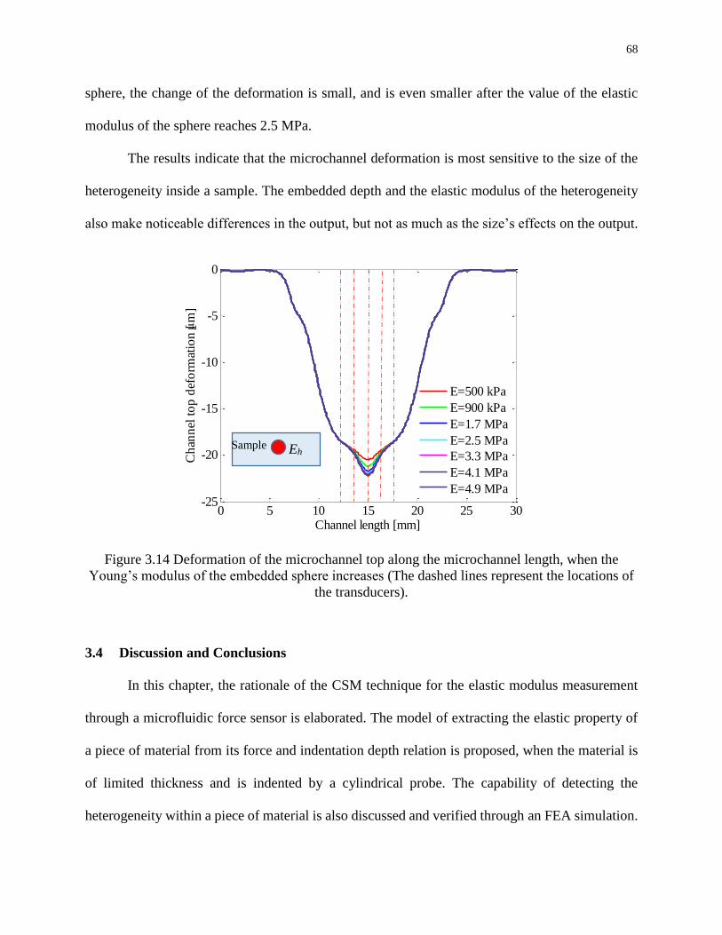
68
sphere, the change of the deformation is small, and is even smaller after the value of the elastic
modulus of the sphere reaches 2.5 MPa.
The results indicate that the microchannel deformation is most sensitive to the size of the
heterogeneity inside a sample. The embedded depth and the elastic modulus of the heterogeneity
also make noticeable differences in the output, but not as much as the size’s effects on the output.
Figure 3.14 Deformation of the microchannel top along the microchannel length, when the
Young’s modulus of the embedded sphere increases (The dashed lines represent the locations of
the transducers).
3.4 Discussion and Conclusions
In this chapter, the rationale of the CSM technique for the elastic modulus measurement
through a microfluidic force sensor is elaborated. The model of extracting the elastic property of
a piece of material from its force and indentation depth relation is proposed, when the material is
of limited thickness and is indented by a cylindrical probe. The capability of detecting the
heterogeneity within a piece of material is also discussed and verified through an FEA simulation.
0 5 10 15 20 25 30-25
-20
-15
-10
-5
0
Channel length [mm]
Ch
ann
el t
op
def
orm
atio
n [
m]
E=500 kPa
E=900 kPa
E=1.7 MPa
E=2.5 MPa
E=3.3 MPa
E=4.1 MPa
E=4.9 MPa
Sample Eh

69
From sweeping three parameters, the depth, radius, and elastic modulus of the hard sphere
representing the heterogeneity in the FEA model, it can be concluded that the size of the
heterogeneity affects the microchannel top deformation the most, which further leads to a larger
change in the voltage output from the corresponding transducer of the device.
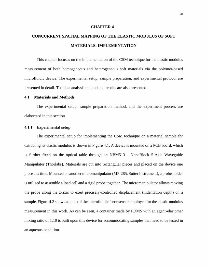
70
CHAPTER 4
CONCURRENT SPATIAL MAPPING OF THE ELASTIC MODULUS OF SOFT
MATERIALS: IMPLEMENTATION
This chapter focuses on the implementation of the CSM technique for the elastic modulus
measurement of both homogeneous and heterogeneous soft materials via the polymer-based
microfluidic device. The experimental setup, sample preparation, and experimental protocol are
presented in detail. The data analysis method and results are also presented.
4.1 Materials and Methods
The experimental setup, sample preparation method, and the experiment process are
elaborated in this section.
4.1.1 Experimental setup
The experimental setup for implementing the CSM technique on a material sample for
extracting its elastic modulus is shown in Figure 4.1. A device is mounted on a PCB board, which
is further fixed on the optical table through an NBM513 - NanoBlock 5-Axis Waveguide
Manipulator (Thorlabs). Materials are cut into rectangular pieces and placed on the device one
piece at a time. Mounted on another micromanipulator (MP-285, Sutter Instrument), a probe holder
is utilized to assemble a load cell and a rigid probe together. The micromanipulator allows moving
the probe along the z-axis to exert precisely-controlled displacement (indentation depth) on a
sample. Figure 4.2 shows a photo of the microfluidic force sensor employed for the elastic modulus
measurement in this work. As can be seen, a container made by PDMS with an agent-elastomer
mixing ratio of 1:10 is built upon this device for accommodating samples that need to be tested in
an aqueous condition.
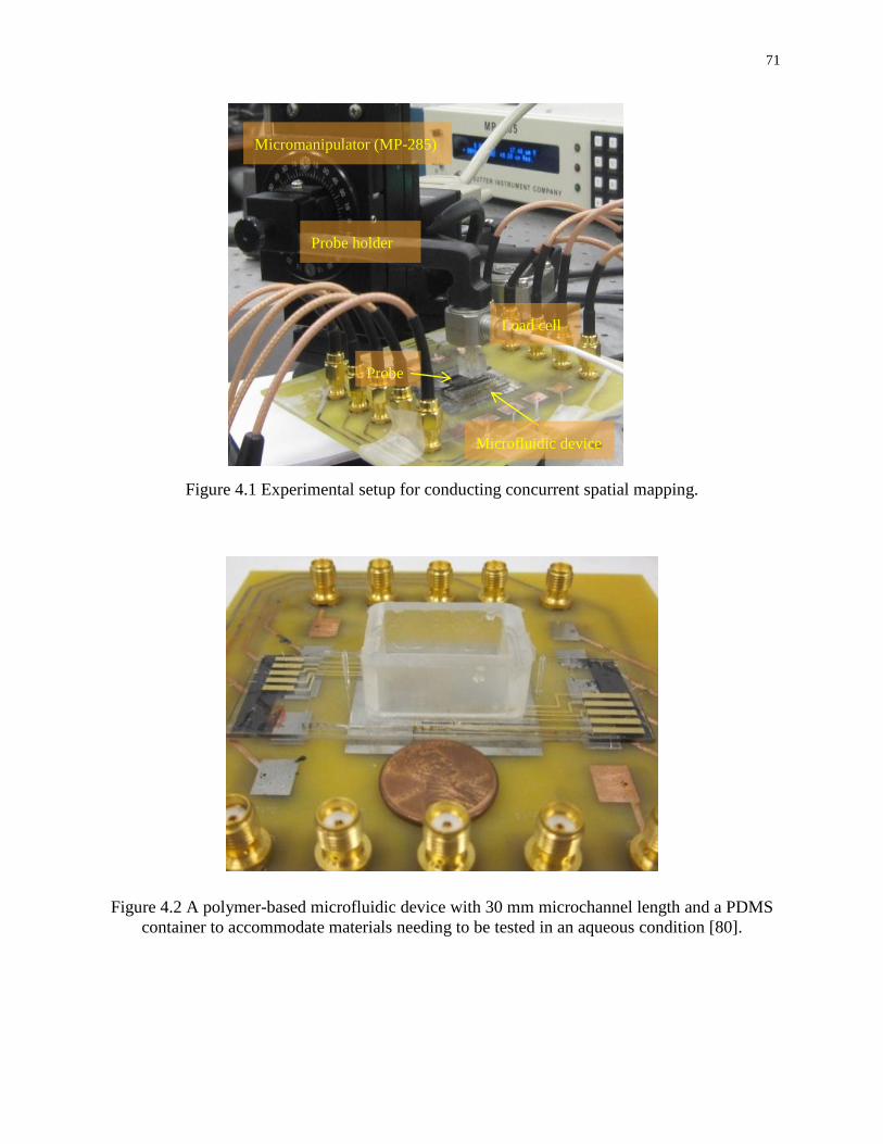
71
Figure 4.1 Experimental setup for conducting concurrent spatial mapping.
Figure 4.2 A polymer-based microfluidic device with 30 mm microchannel length and a PDMS
container to accommodate materials needing to be tested in an aqueous condition [80].
Micromanipulator (MP-285)
Probe holder
Probe
Load cell
Microfluidic device
72
4.1.2 Sample preparation
Both homogeneous and heterogeneous agar samples with an agarose concentration of 1%,
2%, and 3% were prepared in phosphate buffered saline (PBS) from Sigma Aldrich. The solution
was heated to boil and was poured into a Petri dish placed on an optical table and allowed to cool.
The samples were then cut into small pieces and placed in PBS.
Heterogeneous agar samples with the same concentrations were also prepared, with corn
crumbles imbedded. The corn crumbles were about the size of 1 to 2 millimeters, with different
shapes and locations in the agar samples. For preparing the heterogeneous samples, corn crumbles
were placed in the three Petri dishes first, and then solutions of different concentrations were
poured over the crumbles within their respective dishes.
The solidification time for preparing both types of samples was over an hour at room
temperature. Then small pieces of agar samples were cut out with an in-plane dimension of
approximate 10 mm 6 mm. The thickness of the samples was then measured. The samples were
then stored in PBS at room temperature until being tested.
Similar to the preparation of the agar samples, both homogeneous and heterogeneous
PDMS samples were made, as shown in Figure 4.3. The curing agent and the elastomer with the
ratio of 1:30 and 1:40 were poured into two different containers and then thoroughly mixed. For
preparing the homogeneous PDMS samples, the elastomer-agent mixtures with two different
mixing ratios were separately poured into two flat containers being placed on an optical table. For
preparing heterogeneous samples, the mixtures were poured into containers with those scattering
raw corn crumbles mentioned above. The containers were placed on the optical table for over 24
hours to cure before use. Owing to the volume of the mixture being used, the thickness of samples

73
varies from one another. A sample thickness measurement is required for data analysis, and all the
sample thicknesses are presented in Table 4.1.
(a) (b) (c)
Figure 4.3 Prepared (a) 1:30 homogeneous PDMS (b) 1:30 heterogeneous PDMS and (c) 1:40
heterogeneous PDMS samples [80].
Table 4.1 Thickness of the prepared samples.
Sample Thickness
(mm)
1% homogeneous agar 1.954
1% heterogeneous agar 2.638
2% homogeneous agar 2.253
2% heterogeneous agar 2.253
3% homogeneous agar 2.502
3% heterogeneous agar 2.264
1:30 homogeneous PDMS 3.558
1:30 heterogeneous PDMS 3.22
1:40 heterogeneous PDMS 2.849
4.1.3 Experimental protocol
Prior to conducting the CSM on a piece of material to obtain its elastic modulus, a control
experiment on the device is required to acquire its static performance. Specifically, the relation
between the precisely controlled displacement (indentation depth) applied by the cylindrical probe
to the device upper surface and the voltage output from the transducers should be established.
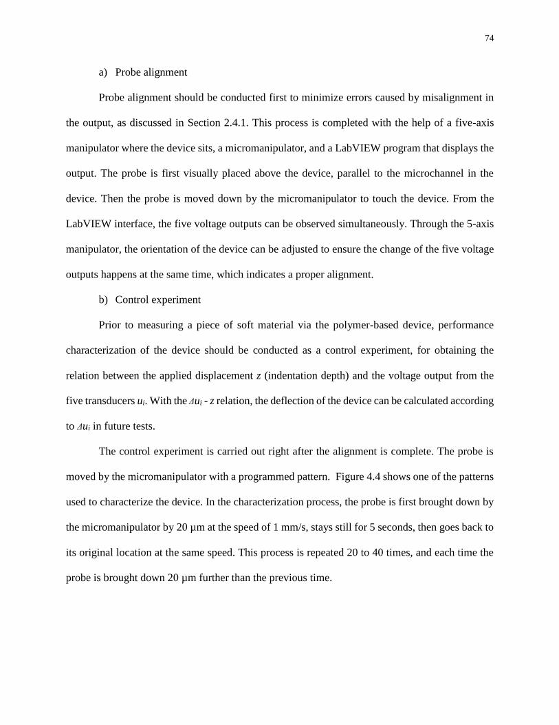
74
a) Probe alignment
Probe alignment should be conducted first to minimize errors caused by misalignment in
the output, as discussed in Section 2.4.1. This process is completed with the help of a five-axis
manipulator where the device sits, a micromanipulator, and a LabVIEW program that displays the
output. The probe is first visually placed above the device, parallel to the microchannel in the
device. Then the probe is moved down by the micromanipulator to touch the device. From the
LabVIEW interface, the five voltage outputs can be observed simultaneously. Through the 5-axis
manipulator, the orientation of the device can be adjusted to ensure the change of the five voltage
outputs happens at the same time, which indicates a proper alignment.
b) Control experiment
Prior to measuring a piece of soft material via the polymer-based device, performance
characterization of the device should be conducted as a control experiment, for obtaining the
relation between the applied displacement z (indentation depth) and the voltage output from the
five transducers ui. With the Δui - z relation, the deflection of the device can be calculated according
to Δui in future tests.
The control experiment is carried out right after the alignment is complete. The probe is
moved by the micromanipulator with a programmed pattern. Figure 4.4 shows one of the patterns
used to characterize the device. In the characterization process, the probe is first brought down by
the micromanipulator by 20 µm at the speed of 1 mm/s, stays still for 5 seconds, then goes back to
its original location at the same speed. This process is repeated 20 to 40 times, and each time the
probe is brought down 20 µm further than the previous time.

75
Figure 4.4 Displacement pattern of the probe for conducting device characterization.
c) CSM for the elastic modulus measurement
After the control experiment is completed, the probe is brought up by the
micromanipulator, to make space for inserting a piece of prepared sample between the device and
the probe. After the material sample is inserted, the probe is brought closer to the sample by the
micromanipulator to identify the contact point. Similar to the alignment process, the contact point
is identified by observing the voltage output from the transducers. The probe is first brought closer
to the sample by the micromanipulator and stops when the distance is closer than 1 mm, judging
by visual examination. Then the probe is brought down by 20 µm each time until an obvious
change in voltage output is observed. The probe is then brought up by 10 µm, and that point is
chosen to be the initial point that the probe and sample start to contact.
0 50 100 150 200-500
-400
-300
-200
-100
0
Time [s]
Pro
be
dis
pla
cem
ent
[m
]
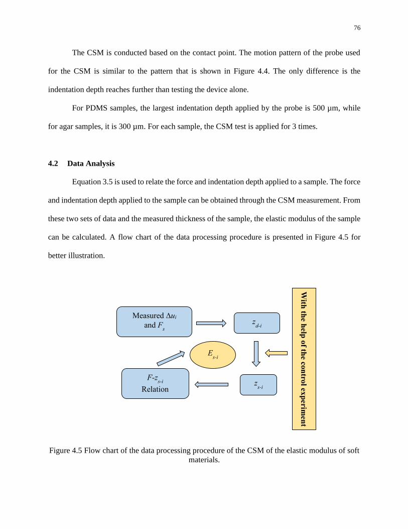
76
The CSM is conducted based on the contact point. The motion pattern of the probe used
for the CSM is similar to the pattern that is shown in Figure 4.4. The only difference is the
indentation depth reaches further than testing the device alone.
For PDMS samples, the largest indentation depth applied by the probe is 500 µm, while
for agar samples, it is 300 µm. For each sample, the CSM test is applied for 3 times.
4.2 Data Analysis
Equation 3.5 is used to relate the force and indentation depth applied to a sample. The force
and indentation depth applied to the sample can be obtained through the CSM measurement. From
these two sets of data and the measured thickness of the sample, the elastic modulus of the sample
can be calculated. A flow chart of the data processing procedure is presented in Figure 4.5 for
better illustration.
Figure 4.5 Flow chart of the data processing procedure of the CSM of the elastic modulus of soft
materials.
Measured ∆ui
and Fs z
d-i
zs-i
F-zs-i
Relation
Es-i
With
the h
elp o
f the co
ntro
l exp
erimen
t
77
As mentioned in Section 3.2, the first direct output of the measurement is the overall load
applied to the sample, which is calculated from the voltage output of the load cell, through a linear
relation. The second output from the measurement is the voltage signals from the five transducers
of the device, which represent the deformation of the device at five discrete locations along the
microchannel length. The overall indentation is predefined as an input value in the LabVIEW
program. According to the conclusion from Chapter 2, the voltage output ui from each transducer
of the device and the indentation applied to the device, z, are linearly related. Thus, the relation
between the indentation depth zdi and the voltage change Δui can be expressed by Equation 4.1.
buaz idi ( 4.1 )
Then the deformation of the device can be acquired by multiplying a constant coefficient
a to the voltage change from its corresponding transducer and adding an intercept b. The
distributed deformation of the device at the locations of the transducers, zdi, is obtained. The
deflection of the material sample at the locations of the five transducers can be calculated
accordingly by Equation 3.6 from the last chapter, zsi = z- zdi. Meanwhile, Equation 3.5 can be
further written as
DFh
Ea
Ea
Fhzsi
)1(12.5
16ln1
2
)1(12.5232.0
3232.0
. ( 4.2 )
A numerical method is applied to solve Equation 4.2, for obtaining the elastic modulus E.
4.3 Results
4.3.1 Device characterization results
From the control experiment, the coefficients to relate the voltage change from each
transducer and the indentation depth as expressed in Equation 4.1 are obtained by a linear curve
fitting and are presented in Table 4.2. The negative sign of coefficient a in Table 4.2 indicates that
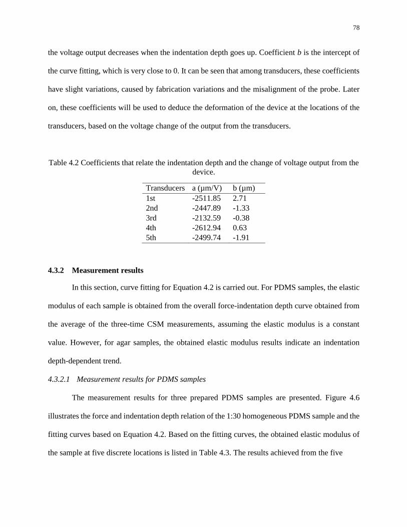
78
the voltage output decreases when the indentation depth goes up. Coefficient b is the intercept of
the curve fitting, which is very close to 0. It can be seen that among transducers, these coefficients
have slight variations, caused by fabrication variations and the misalignment of the probe. Later
on, these coefficients will be used to deduce the deformation of the device at the locations of the
transducers, based on the voltage change of the output from the transducers.
Table 4.2 Coefficients that relate the indentation depth and the change of voltage output from the
device.
Transducers a (µm/V) b (µm)
1st -2511.85 2.71
2nd -2447.89 -1.33
3rd -2132.59 -0.38
4th -2612.94 0.63
5th -2499.74 -1.91
4.3.2 Measurement results
In this section, curve fitting for Equation 4.2 is carried out. For PDMS samples, the elastic
modulus of each sample is obtained from the overall force-indentation depth curve obtained from
the average of the three-time CSM measurements, assuming the elastic modulus is a constant
value. However, for agar samples, the obtained elastic modulus results indicate an indentation
depth-dependent trend.
4.3.2.1 Measurement results for PDMS samples
The measurement results for three prepared PDMS samples are presented. Figure 4.6
illustrates the force and indentation depth relation of the 1:30 homogeneous PDMS sample and the
fitting curves based on Equation 4.2. Based on the fitting curves, the obtained elastic modulus of
the sample at five discrete locations is listed in Table 4.3. The results achieved from the five
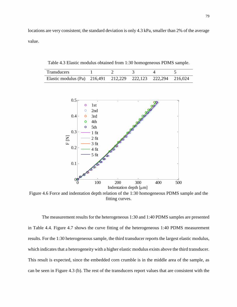
79
locations are very consistent; the standard deviation is only 4.3 kPa, smaller than 2% of the average
value.
Table 4.3 Elastic modulus obtained from 1:30 homogeneous PDMS sample.
Transducers 1 2 3 4 5
Elastic modulus (Pa) 216,491 212,229 222,123 222,294 216,024
Figure 4.6 Force and indentation depth relation of the 1:30 homogeneous PDMS sample and the
fitting curves.
The measurement results for the heterogeneous 1:30 and 1:40 PDMS samples are presented
in Table 4.4. Figure 4.7 shows the curve fitting of the heterogeneous 1:40 PDMS measurement
results. For the 1:30 heterogeneous sample, the third transducer reports the largest elastic modulus,
which indicates that a heterogeneity with a higher elastic modulus exists above the third transducer.
This result is expected, since the embedded corn crumble is in the middle area of the sample, as
can be seen in Figure 4.3 (b). The rest of the transducers report values that are consistent with the
0 100 200 300 400 5000
0.1
0.2
0.3
0.4
0.5
Indentation depth [m]
F [
N]
1st
2nd
3rd
4th
5th
1 fit
2 fit
3 fit
4 fit
5 fit
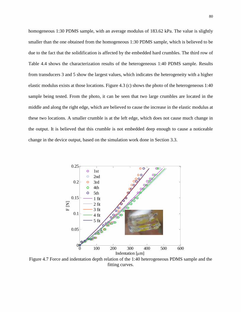
80
homogeneous 1:30 PDMS sample, with an average modulus of 183.62 kPa. The value is slightly
smaller than the one obtained from the homogeneous 1:30 PDMS sample, which is believed to be
due to the fact that the solidification is affected by the embedded hard crumbles. The third row of
Table 4.4 shows the characterization results of the heterogeneous 1:40 PDMS sample. Results
from transducers 3 and 5 show the largest values, which indicates the heterogeneity with a higher
elastic modulus exists at those locations. Figure 4.3 (c) shows the photo of the heterogeneous 1:40
sample being tested. From the photo, it can be seen that two large crumbles are located in the
middle and along the right edge, which are believed to cause the increase in the elastic modulus at
these two locations. A smaller crumble is at the left edge, which does not cause much change in
the output. It is believed that this crumble is not embedded deep enough to cause a noticeable
change in the device output, based on the simulation work done in Section 3.3.
Figure 4.7 Force and indentation depth relation of the 1:40 heterogeneous PDMS sample and the
fitting curves.
0 100 200 300 400 500 6000
0.05
0.1
0.15
0.2
0.25
Indentation [m]
F [
N]
1st
2nd
3rd
4th
5th
1 fit
2 fit
3 fit
4 fit
5 fit

81
Table 4.4 Elastic modulus obtained from the 1:30 and 1:40 heterogeneous PDMS samples
through CSM.
1st 2nd 3rd 4th 5th
1:30 heterogeneous (Pa) 185,682 166,514 252,861 175,485 206,796
1:40 heterogeneous (Pa) 84,348 79,610 102,985 80,877 104,963
Table 4.5 Measured elastic modulus of PDMS with 1:30 and 1:40 mixing ratios in the literature.
PDMS [81] [82] [83] [84] [85] [86]
1:30 N/A 0.42~1.53
MPa
304.6 kPa ~200 kPa 270 kPa N/A
1:40 78 kPa N/A 97.6 kPa 41.89 kPa N/A 0.1 MPa
Table 4.5 presents the measurement results of 1:30 and 1:40 homogeneous PDMS samples
from the literature review. The methods being used to achieve the results include nanoindentation
[85], cyclic unconfined compression testing [83], and uniaxial mechanical characterization [84],
etc. By comparing the PDMS elastic modulus measured by this experimental technique and the
results obtained by other groups, it can be seen that the results are within the right range, which
further indicates the reliability of the CSM technique for the elastic modulus measurement through
a microfluidic device.
4.3.2.2 Measurement results for Agar samples
In this section, the measurement results for agar samples are presented. Unlike the PDMS
samples, the agar samples exhibit a more obvious indentation depth-dependent property. A similar
phenomenon was observed in biological tissues, as the modulus is dependent on the strain level
[29]. In this case, instead of obtaining an overall elastic modulus through a regression method, the
elastic modulus at each indentation depth is calculated. Since agar samples were tested in an
aqueous condition, it took longer to achieve its steady state. Thus, to achieve a relatively stable

82
result, the data used in the data analysis are those after 5 seconds relaxation in each indentation.
Figure 4.8 shows the measured elastic modulus of the homogeneous 1%, 2%, and 3% agar
samples at different indentation depths with error bars. Table 4.6 summarizes the results obtained
from Figure 4.8.
(a)
(b)
Figure 4.8 Measured elastic modulus of the homogeneous (a) 1% agar, (b) 2% agar, and (c) 3%
agar samples as a function of indentation depth.
50 100 150 200 250 300 3501.5
2
2.5
3
3.5
4
4.5
5
5.5x 10
4
Indentation depth [m]
E [
Pa]
1st
2nd
3rd
4th
5th
0 100 200 300 400 500 6000.4
0.6
0.8
1
1.2
1.4
1.6
1.8x 10
5
Indentation depth [m]
E [
Pa]
1st
2nd
3rd
4th
5th
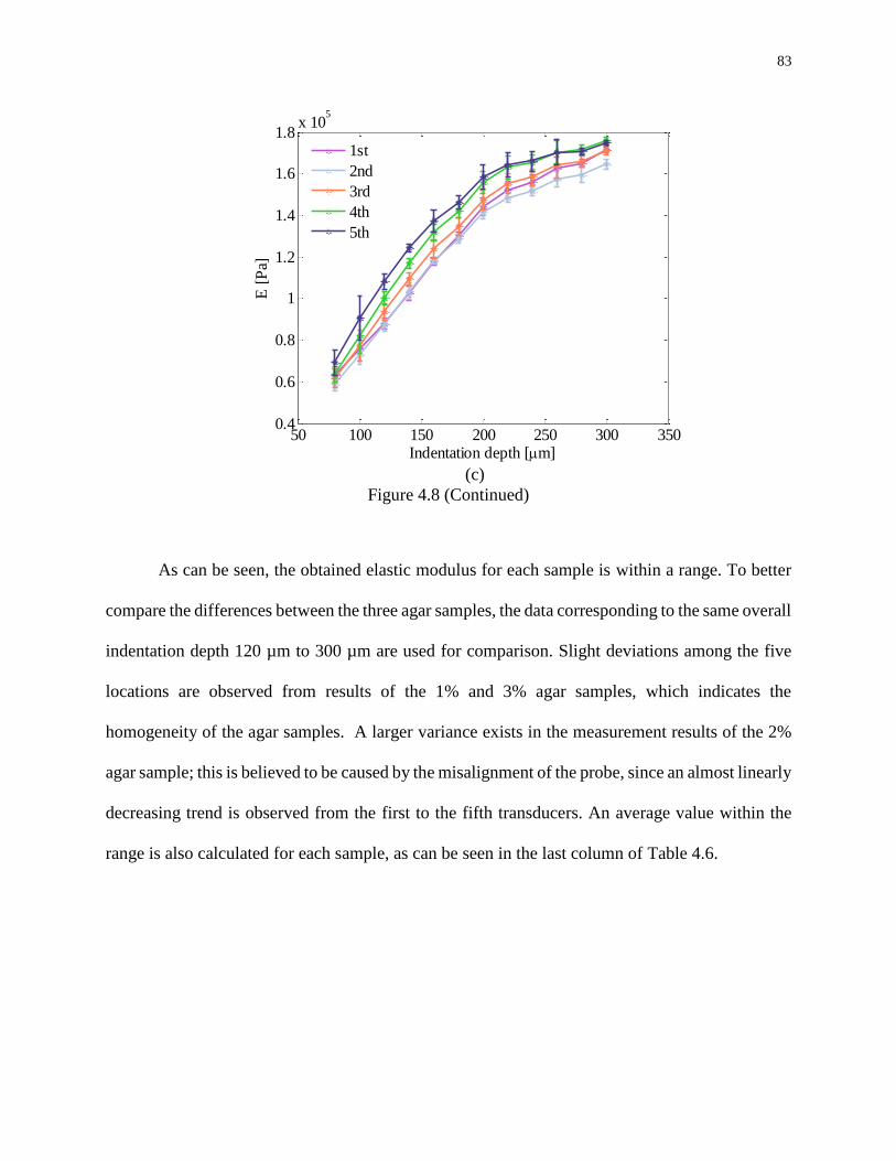
83
(c)
Figure 4.8 (Continued)
As can be seen, the obtained elastic modulus for each sample is within a range. To better
compare the differences between the three agar samples, the data corresponding to the same overall
indentation depth 120 µm to 300 µm are used for comparison. Slight deviations among the five
locations are observed from results of the 1% and 3% agar samples, which indicates the
homogeneity of the agar samples. A larger variance exists in the measurement results of the 2%
agar sample; this is believed to be caused by the misalignment of the probe, since an almost linearly
decreasing trend is observed from the first to the fifth transducers. An average value within the
range is also calculated for each sample, as can be seen in the last column of Table 4.6.
50 100 150 200 250 300 3500.4
0.6
0.8
1
1.2
1.4
1.6
1.8x 10
5
Indentation depth [m]
E [
Pa]
1st
2nd
3rd
4th
5th
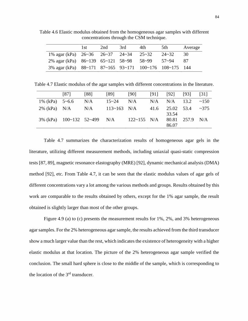
84
Table 4.6 Elastic modulus obtained from the homogeneous agar samples with different
concentrations through the CSM technique.
1st 2nd 3rd 4th 5th Average
1% agar (kPa) 26~36 26~37 24~34 25~32 24~32 30
2% agar (kPa) 86~139 65~121 58~98 58~99 57~94 87
3% agar (kPa) 88~171 87~165 93~171 100~176 108~175 144
Table 4.7 Elastic modulus of the agar samples with different concentrations in the literature.
[87] [88] [89] [90] [91] [92] [93] [31]
1% (kPa) 5~6.6 N/A 15~24 N/A N/A N/A 13.2 ~150
2% (kPa) N/A N/A 113~163 N/A 41.6 25.02
33.54
53.4 ~375
3% (kPa) 100~132 52~499 N/A 122~155 N/A 80.81
86.07
257.9 N/A
Table 4.7 summarizes the characterization results of homogeneous agar gels in the
literature, utilizing different measurement methods, including uniaxial quasi-static compression
tests [87, 89], magnetic resonance elastography (MRE) [92], dynamic mechanical analysis (DMA)
method [92], etc. From Table 4.7, it can be seen that the elastic modulus values of agar gels of
different concentrations vary a lot among the various methods and groups. Results obtained by this
work are comparable to the results obtained by others, except for the 1% agar sample, the result
obtained is slightly larger than most of the other groups.
Figure 4.9 (a) to (c) presents the measurement results for 1%, 2%, and 3% heterogeneous
agar samples. For the 2% heterogeneous agar sample, the results achieved from the third transducer
show a much larger value than the rest, which indicates the existence of heterogeneity with a higher
elastic modulus at that location. The picture of the 2% heterogeneous agar sample verified the
conclusion. The small hard sphere is close to the middle of the sample, which is corresponding to
the location of the 3rd transducer.
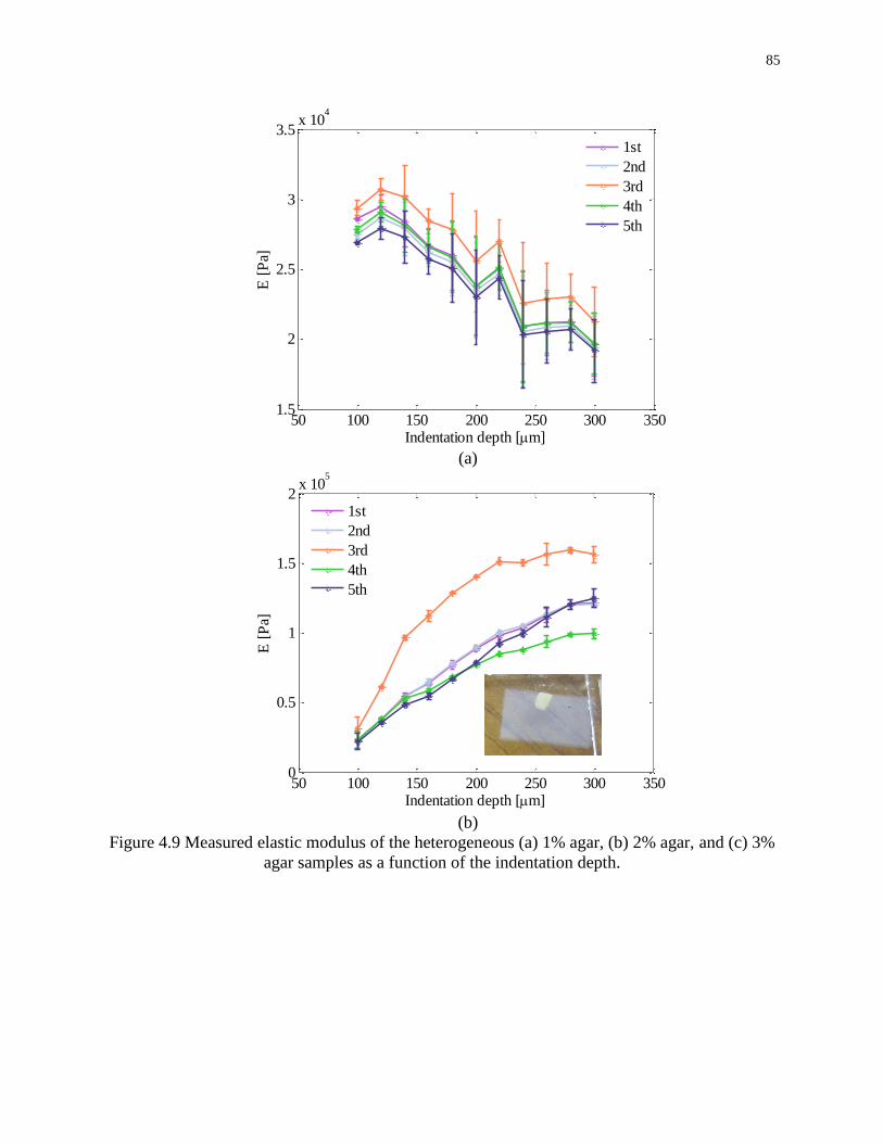
85
(a)
(b)
Figure 4.9 Measured elastic modulus of the heterogeneous (a) 1% agar, (b) 2% agar, and (c) 3%
agar samples as a function of the indentation depth.
50 100 150 200 250 300 3501.5
2
2.5
3
3.5x 10
4
Indentation depth [m]
E [
Pa]
1st
2nd
3rd
4th
5th
50 100 150 200 250 300 3500
0.5
1
1.5
2x 10
5
Indentation depth [m]
E [
Pa]
1st
2nd
3rd
4th
5th
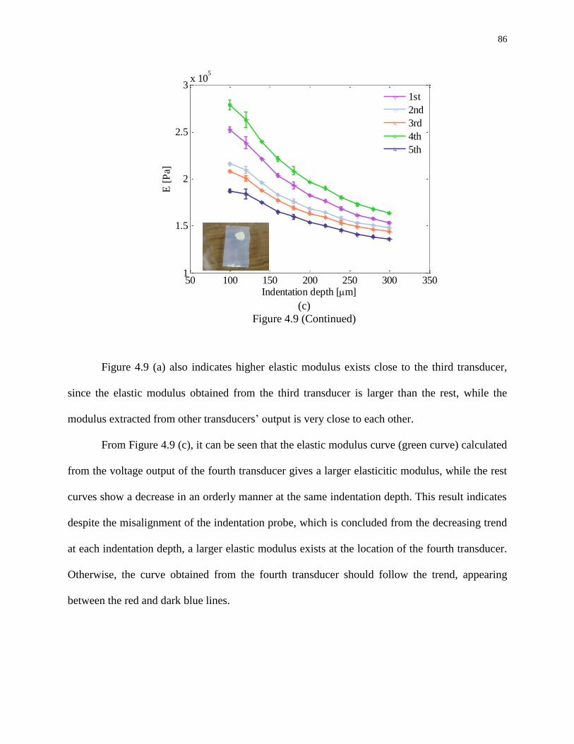
86
(c)
Figure 4.9 (Continued)
Figure 4.9 (a) also indicates higher elastic modulus exists close to the third transducer,
since the elastic modulus obtained from the third transducer is larger than the rest, while the
modulus extracted from other transducers’ output is very close to each other.
From Figure 4.9 (c), it can be seen that the elastic modulus curve (green curve) calculated
from the voltage output of the fourth transducer gives a larger elasticitic modulus, while the rest
curves show a decrease in an orderly manner at the same indentation depth. This result indicates
despite the misalignment of the indentation probe, which is concluded from the decreasing trend
at each indentation depth, a larger elastic modulus exists at the location of the fourth transducer.
Otherwise, the curve obtained from the fourth transducer should follow the trend, appearing
between the red and dark blue lines.
50 100 150 200 250 300 3501
1.5
2
2.5
3x 10
5
Indentation depth [m]
E [
Pa]
1st
2nd
3rd
4th
5th
87
4.4 Discussion and Conclusions
For simplicity, many assumptions are made for extracting the elastic modulus of the soft
materials. First, it is assumed that the deformation of the testing materials is still in their linear
regime, which means the strain level is within 5% to 10%. Secondly, it is assumed that the material
follows elastic deformation rules. However, many other models are adopted to better describe the
elastic property of soft materials, since most bio-materials start to have nonlinear behavior at
higher strain rate. For example, hyperelastic material models have been used to model joint
cartilage. Other models include neo-Hookean, Mooney-Rivlin, Saint-Venant Kirchhoff, Arruda-
Boyce, Ogden, etc. These models could be considered for incorporation into Equation 4.2 in future
work.
Overall, this chapter presents the implementation of the CSM technique on the elasticitic
modulus measurement of both homogeneous and heterogeneous synthetic materials. The
measurement results agree well with those presented in the literature. The capability of the device
to measure the spatially-varying elastic modulus of soft materials through one measurement is
successfully proved.
88
CHAPTER 5
CONCURRENT SPATIAL MAPPING OF THE LOSS MODULUS OF SOFT
MATERIALS: THEORY
The viscoelastic behavior of a material is usually studied through the creep test, relaxation
test and harmonic test. It has been successfully proven that the polymer-based microfluidic device
is capable of detecting the spatially-varying viscous behavior of a material through a relaxation
test [94]. This chapter and the following chapter explore the feasibility of measuring the viscous
property of a material through decoupling its stiffness and damping coefficient from two sets of
system-level parameters measured by the harmonic test, and estimate its spatially-varying loss
modulus through the spatially-varying phase shifts. This chapter first presents the rationale related
to the CSM of the viscoelastic behavior of soft materials via the polymer-based microfluidic
device. Then, the derivation of relating the damping coefficient to the loss modulus of a material
is presented. The experimental implementation will be provided in the next chapter.
5.1 Rationale
When a piece of material is under a sinusoidal loading, the response of the material, the
phase shift in particular, can be used to detect the viscosity within a material. In Figure 5.1, the
phase shifts between stress and strain in three different scenarios are illustrated. When the material
is purely elastic, the stress and strain are completely in phase, while a viscous material gives an
out-of-phase response. For viscoelastic materials, the phase lag is between 0 to 90°[95]. As such,
phase shifts between the applied load and the corresponding deflection can manifest the viscous
property of materials.
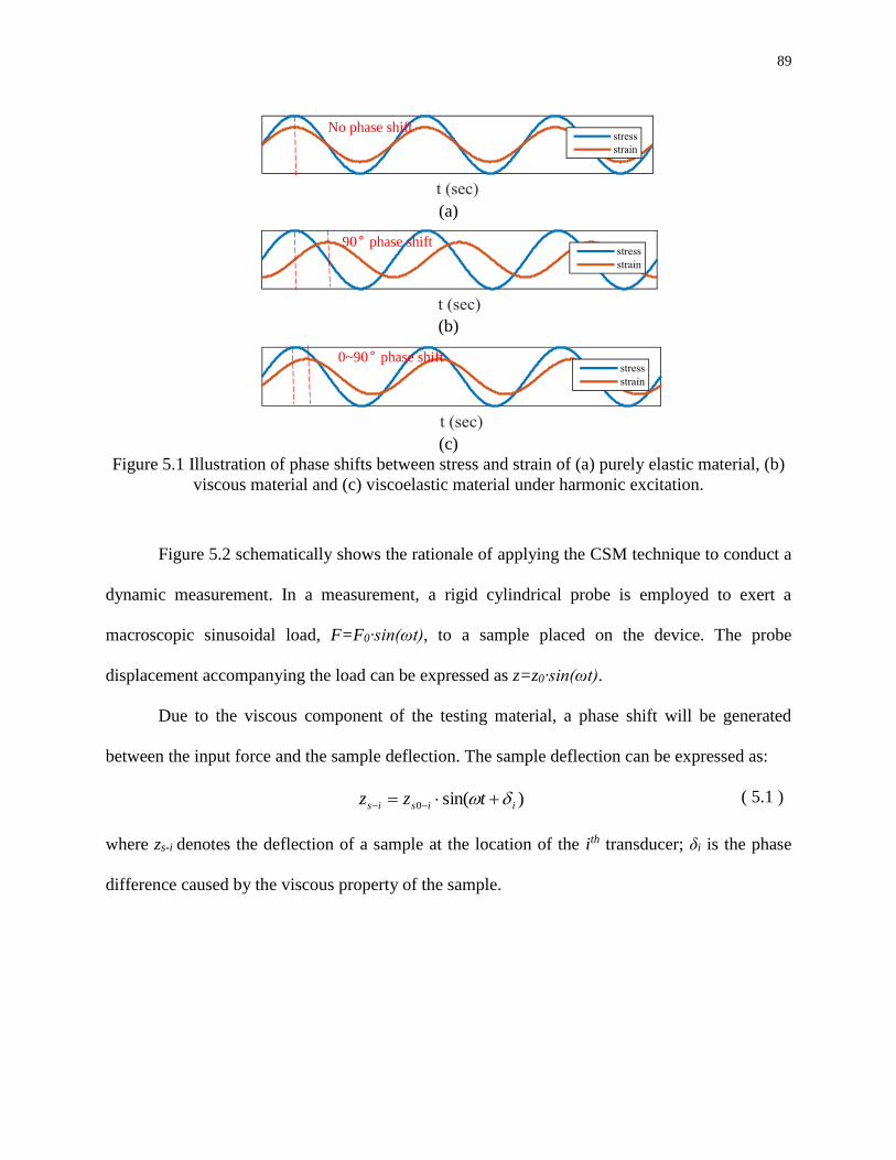
89
(a)
(b)
(c)
Figure 5.1 Illustration of phase shifts between stress and strain of (a) purely elastic material, (b)
viscous material and (c) viscoelastic material under harmonic excitation.
Figure 5.2 schematically shows the rationale of applying the CSM technique to conduct a
dynamic measurement. In a measurement, a rigid cylindrical probe is employed to exert a
macroscopic sinusoidal load, F=F0·sin(ωt), to a sample placed on the device. The probe
displacement accompanying the load can be expressed as z=z0·sin(ωt).
Due to the viscous component of the testing material, a phase shift will be generated
between the input force and the sample deflection. The sample deflection can be expressed as:
)sin(0 iisis tzz ( 5.1 )
where zs-i denotes the deflection of a sample at the location of the ith transducer; δi is the phase
difference caused by the viscous property of the sample.
No phase shift
90° phase shift
0~90° phase shift
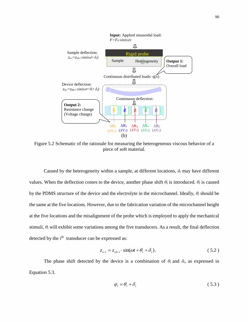
90
(b)
Figure 5.2 Schematic of the rationale for measuring the heterogeneous viscous behavior of a
piece of soft material.
Caused by the heterogeneity within a sample, at different locations, δi may have different
values. When the deflection comes to the device, another phase shift θi is introduced. θi is caused
by the PDMS structure of the device and the electrolyte in the microchannel. Ideally, θi should be
the same at the five locations. However, due to the fabrication variation of the microchannel height
at the five locations and the misalignment of the probe which is employed to apply the mechanical
stimuli, θi will exhibit some variations among the five transducers. As a result, the final deflection
detected by the ith transducer can be expressed as:
)sin(0 iiisis tzz . ( 5.2 )
The phase shift detected by the device is a combination of θi and δi, as expressed in
Equation 5.3.
iii ( 5.3 )
(V1) (V2) (V3) (V4) (V5)
Rigid probe
Input: Applied sinusoidal load:
F=F0·sin(ωt)
Continuous distributed loads: q(x)
Continuous deflection:
Sample Output 1: Overall load
R1 R2 R3 R4 R5
Output 2: Resistance change
(Voltage change)
Sample deflection:
zs-i=zs0-i·sin(ωt+δi)
Device deflection:
zd-i=zd0-i·sin(ωt+θi+δi)
Heterogeneity
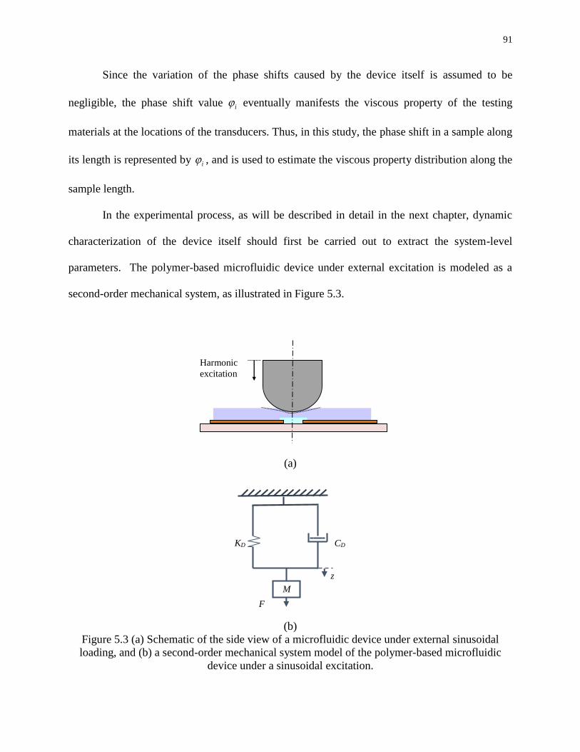
91
Since the variation of the phase shifts caused by the device itself is assumed to be
negligible, the phase shift value i eventually manifests the viscous property of the testing
materials at the locations of the transducers. Thus, in this study, the phase shift in a sample along
its length is represented by i , and is used to estimate the viscous property distribution along the
sample length.
In the experimental process, as will be described in detail in the next chapter, dynamic
characterization of the device itself should first be carried out to extract the system-level
parameters. The polymer-based microfluidic device under external excitation is modeled as a
second-order mechanical system, as illustrated in Figure 5.3.
(a)
(b)
Figure 5.3 (a) Schematic of the side view of a microfluidic device under external sinusoidal
loading, and (b) a second-order mechanical system model of the polymer-based microfluidic
device under a sinusoidal excitation.
Harmonic
excitation
KD CD
F
z
M
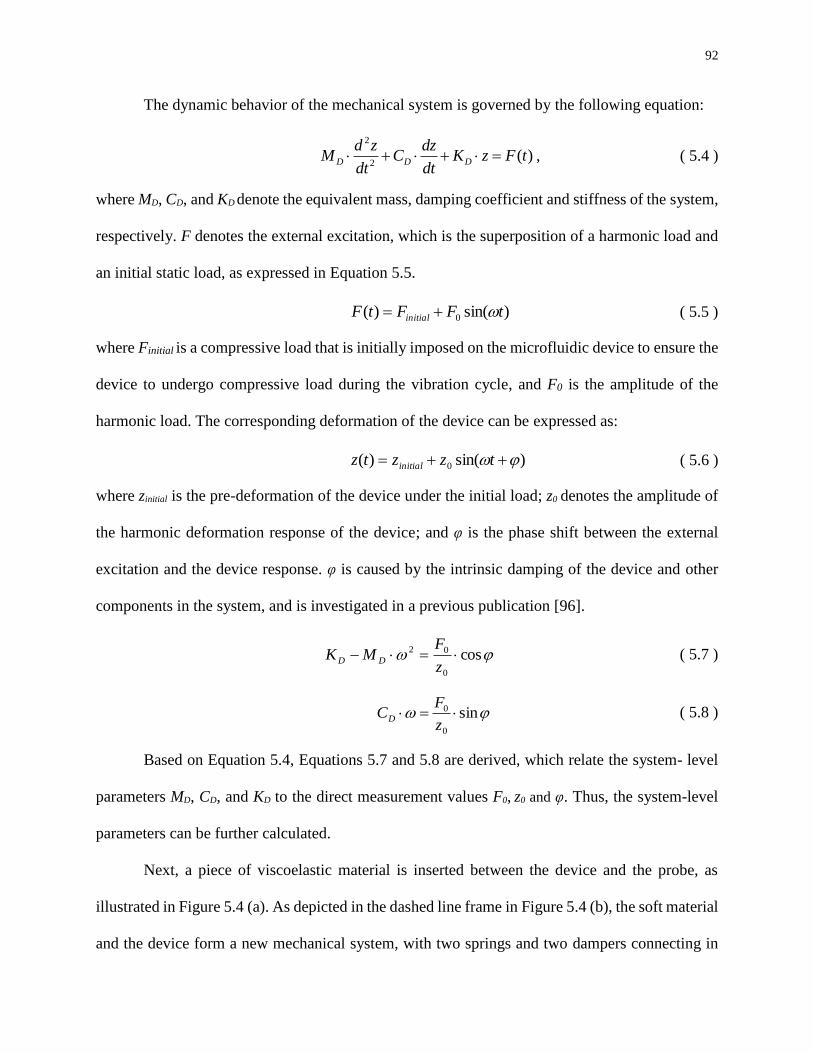
92
The dynamic behavior of the mechanical system is governed by the following equation:
)(2
2
tFzKdt
dzC
dt
zdM DDD , ( 5.4 )
where MD, CD, and KD denote the equivalent mass, damping coefficient and stiffness of the system,
respectively. F denotes the external excitation, which is the superposition of a harmonic load and
an initial static load, as expressed in Equation 5.5.
)sin()( 0 tFFtF initial ( 5.5 )
where Finitial is a compressive load that is initially imposed on the microfluidic device to ensure the
device to undergo compressive load during the vibration cycle, and F0 is the amplitude of the
harmonic load. The corresponding deformation of the device can be expressed as:
)sin()( 0 tzztz initial ( 5.6 )
where zinitial is the pre-deformation of the device under the initial load; z0 denotes the amplitude of
the harmonic deformation response of the device; and φ is the phase shift between the external
excitation and the device response. φ is caused by the intrinsic damping of the device and other
components in the system, and is investigated in a previous publication [96].
cos0
02 z
FMK DD ( 5.7 )
sin0
0 z
FCD
( 5.8 )
Based on Equation 5.4, Equations 5.7 and 5.8 are derived, which relate the system- level
parameters MD, CD, and KD to the direct measurement values F0, z0 and φ. Thus, the system-level
parameters can be further calculated.
Next, a piece of viscoelastic material is inserted between the device and the probe, as
illustrated in Figure 5.4 (a). As depicted in the dashed line frame in Figure 5.4 (b), the soft material
and the device form a new mechanical system, with two springs and two dampers connecting in
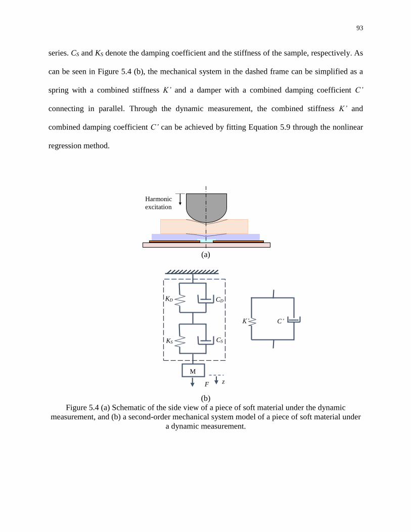
93
series. CS and KS denote the damping coefficient and the stiffness of the sample, respectively. As
can be seen in Figure 5.4 (b), the mechanical system in the dashed frame can be simplified as a
spring with a combined stiffness K’ and a damper with a combined damping coefficient C’
connecting in parallel. Through the dynamic measurement, the combined stiffness K’ and
combined damping coefficient C’ can be achieved by fitting Equation 5.9 through the nonlinear
regression method.
(a)
(b)
Figure 5.4 (a) Schematic of the side view of a piece of soft material under the dynamic
measurement, and (b) a second-order mechanical system model of a piece of soft material under
a dynamic measurement.
Harmonic
excitation
KD
KS
CD
CS
z
M
K’ C’
F

94
2222
0
0
')''(
1
CMKF
z ( 5.9 )
To decouple the material properties of the test material from the combined stiffness and
damping coefficient, Equations 5.10 and 5.11 are applied.
D
S
KK
K1
'
1
1
( 5.10 )
D
S
CC
C1
'
1
1
( 5.11 )
5.2 Relation between the Loss Modulus and the Damping Coefficient
The energy loss in a material sample within one harmonic vibration cycle can be expressed
as:
dtxCdxxCdxFW dd
2
( 5.12 )
where Fd denotes the damping force; C denotes the damping coefficient of the material; and x
denotes the harmonic displacement imposed on the sample.
The imposed displacement on the sample can be expressed as:
)sin( tXx ( 5.13 )
where X denotes the displacement amplitude and φ is the phase between the displacement and the
harmonic force input.
The vibration velocity applied to the sample can be expressed as the first derivative of the
imposed displacement, as expressed in Equation 5.14.
)cos( tXx ( 5.14 )

95
Thus, the energy dissipation during one vibration cycle can be further written into:
2
2
0
2222 )(cos XCdttXCdtxCdxxCdxFW dd
( 5.15 )
Assuming the cyclic force is uniformly applied to a material sample in a bulk shape, the
stress and strain distributions are considered to be uniform throughout the entire material. Then
the energy loss can be expressed as:
dVdtdt
ddVdW
Tt
t
Tt
td
1
1 . ( 5.16 )
The stress, strain, and their relation can be further written into Equations 5.17 to 5.19:
A
eFe
ti
ti
0
0
( 5.17 )
)()(
0
titi eh
Xe
( 5.18 )
)( EiEE ( 5.19 )
where A and h denote the cross section area and the thickness of the material sample, respectively;
E is the complex modulus.
The complex modulus can be further written into:
sincos 00
0
0
AX
hFi
AX
hFEiEeE i
. ( 5.20 )
The real part of the strain and stress can be expressed as:
)cos(0 tR ( 5.21 )
)cos(0 tR
( 5.22 )
Then, the energy loss per unit volume during a vibration cycle can be expressed as:
96
1 1
1 1
1
1
1
1
0
0
0 0
cos( ) sin
cos( )sin
sinsin
t T t TR
d R R Rt t
t T
t
t T
t
dw d dt
dt
F Xt t dt
A h
F Xt t dt
Ah
F X F X
Ah Ah
( 5.23 )
For the entire sample, the energy loss per cycle can be expressed as:
222
0
0 sinsin XCAh
XE
h
AX
AX
hFXFdVwW dd
( 5.24 )
From here, the loss modulus can be related to the damping coefficient as:
A
hCE
( 5.25 )
Equation 5.25 calculates the overall loss modulus of a material. In conjunction with the
obtained phase shifts along the sample length, the distribution of the loss modulus along the sample
length can be estimated.
According to Equation 5.20, the relation between the storage modulus and loss modulus
can be expressed as
tan
E
E. ( 5.26 )
Thus the storage modulus can be written into:
tan
EE
. ( 5.27 )
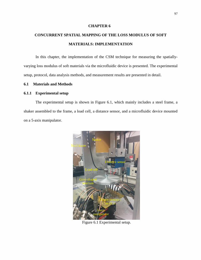
97
CHAPTER 6
CONCURRENT SPATIAL MAPPING OF THE LOSS MODULUS OF SOFT
MATERIALS: IMPLEMENTATION
In this chapter, the implementation of the CSM technique for measuring the spatially-
varying loss modulus of soft materials via the microfluidic device is presented. The experimental
setup, protocol, data analysis methods, and measurement results are presented in detail.
6.1 Materials and Methods
6.1.1 Experimental setup
The experimental setup is shown in Figure 6.1, which mainly includes a steel frame, a
shaker assembled to the frame, a load cell, a distance sensor, and a microfluidic device mounted
on a 5-axis manipulator.
Figure 6.1 Experimental setup.
Distance sensor
Shaker
Steel frame
Load cell
Cone-shaped
structure
Device mounted
on PCB
5-axis
manipulator
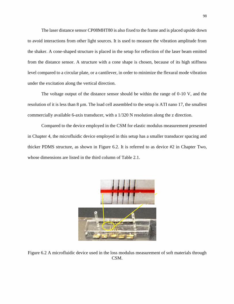
98
The laser distance sensor CP08MHT80 is also fixed to the frame and is placed upside down
to avoid interactions from other light sources. It is used to measure the vibration amplitude from
the shaker. A cone-shaped structure is placed in the setup for reflection of the laser beam emitted
from the distance sensor. A structure with a cone shape is chosen, because of its high stiffness
level compared to a circular plate, or a cantilever, in order to minimize the flexural mode vibration
under the excitation along the vertical direction.
The voltage output of the distance sensor should be within the range of 0-10 V, and the
resolution of it is less than 8 µm. The load cell assembled to the setup is ATI nano 17, the smallest
commercially available 6-axis transducer, with a 1/320 N resolution along the z direction.
Compared to the device employed in the CSM for elastic modulus measurement presented
in Chapter 4, the microfluidic device employed in this setup has a smaller transducer spacing and
thicker PDMS structure, as shown in Figure 6.2. It is referred to as device #2 in Chapter Two,
whose dimensions are listed in the third column of Table 2.1.
Figure 6.2 A microfluidic device used in the loss modulus measurement of soft materials through
CSM.
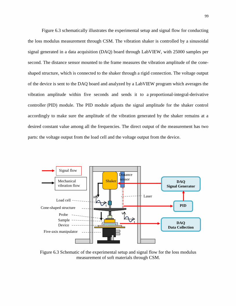
99
Figure 6.3 schematically illustrates the experimental setup and signal flow for conducting
the loss modulus measurement through CSM. The vibration shaker is controlled by a sinusoidal
signal generated in a data acquisition (DAQ) board through LabVIEW, with 25000 samples per
second. The distance sensor mounted to the frame measures the vibration amplitude of the cone-
shaped structure, which is connected to the shaker through a rigid connection. The voltage output
of the device is sent to the DAQ board and analyzed by a LabVIEW program which averages the
vibration amplitude within five seconds and sends it to a proportional-integral-derivative
controller (PID) module. The PID module adjusts the signal amplitude for the shaker control
accordingly to make sure the amplitude of the vibration generated by the shaker remains at a
desired constant value among all the frequencies. The direct output of the measurement has two
parts: the voltage output from the load cell and the voltage output from the device.
Figure 6.3 Schematic of the experimental setup and signal flow for the loss modulus
measurement of soft materials through CSM.
PID
DAQ
Signal Generator
z
t
DAQ
Data Collection
v
t
Load cell
Cone-shaped structure
Probe
Sample
Device
Five-axis manipulator
Signal flow
Mechanical
vibration flow
Laser
Distance
sensor Shaker

100
The load cell is connected between the vibration shaker and the cone-shaped laser reflector
which also accounts for the majority of the equivalent mass of the vibration system. The device is
placed on the five-axis manipulator which helps adjust the orientation of the device to achieve
better alignment. A block with a cylinder probe is connected to the laser reflector, which is used
to exert the amplitude-demodulated vibration to a sample placed on the device. The output from
the load cell and the device is recorded by the DAQ board through another LabVIEW program.
The sampling rate is set to be 5000 for all the dynamic measurement with this setup.
6.1.2 Sample preparation
In the measurement, materials obtained from Smooth-on Inc. are used as the homogeneous
material samples. PDMS with a 1:30 agent to base mixing ratio is used as the matrix material for
making heterogeneous samples. Similarly, heterogeneity is created by embedding corn crumbles
into the PDMS samples. The dimensions of the samples are shown in Table 6.1.
The photos of the testing samples are shown in Figure 6.4. As can be seen, the samples
were cut into rectangular prisms, yet the dimensions vary from sample to sample.
Table 6.1 Dimensions of the testing samples.
Sample name Dimensions (mm)
l×w×h
Dragon skin pro 8.13×5.59×3.56
Dragon skin 10 9.40×5.10×2.54
Dragon skin 20 9.10×5.10×3.81
Ecoflex 8.89×5.33×3.30
1:30 PDMS 1 12.95×4.83×3.05
1:30 PDMS 2 8.38×4.06×3.05
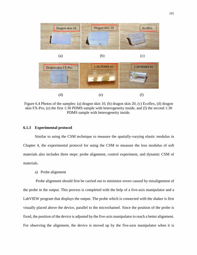
101
(a) (b) (c)
(d) (e) (f)
Figure 6.4 Photos of the samples: (a) dragon skin 10, (b) dragon skin 20, (c) Ecoflex, (d) dragon
skin FX-Pro, (e) the first 1:30 PDMS sample with heterogeneity inside, and (f) the second 1:30
PDMS sample with heterogeneity inside.
6.1.3 Experimental protocol
Similar to using the CSM technique to measure the spatially-varying elastic modulus in
Chapter 4, the experimental protocol for using the CSM to measure the loss modulus of soft
materials also includes three steps: probe alignment, control experiment, and dynamic CSM of
materials.
a) Probe alignment
Probe alignment should first be carried out to minimize errors caused by misalignment of
the probe in the output. This process is completed with the help of a five-axis manipulator and a
LabVIEW program that displays the output. The probe which is connected with the shaker is first
visually placed above the device, parallel to the microchannel. Since the position of the probe is
fixed, the position of the device is adjusted by the five-axis manipulator to reach a better alignment.
For observing the alignment, the device is moved up by the five-axis manipulator when it is
Dragon skin 10 Dragon skin 20 Ecoflex
Dragon skin FX-Pro 1:30 PDMS #1 1:30 PDMS #2

102
approximately 0.5 mm away from the probe until it is in touch with the probe. At the same time,
the output signals from the five transducers of the device are recorded by the LabVIEW program
and exhibited on the screen in the LabVIEW front panel. Through the five-axis manipulator, the
orientation of the device is further adjusted to make sure the change of the five voltage outputs
happens at the same time, which indicates a proper alignment. After the orientation is fixed, the
device is brought down, so that no initial deformation is applied to the device at this stage.
Although the misalignment of a probe is alleviated by using voltage change in the
calculation for obtaining the elastic property of a material, as mentioned in Section 2.4 and Chapter
4, it has a larger effect on the phase shift.
Evidently, a better alignment will improve the accuracy and reproducibility of the
measured results. Although great care has been taken to conduct the probe alignment,
misalignment still more or less exists.
b) Control experiment
A control experiment is conducted on the device itself prior to measuring a sample, in order
to extract the system-level parameters for future use. Since the device itself is a damped mechanical
system, it is expected to observe a phase shift between the load input and the voltage output of the
device.
After the alignment is finished, the device is brought up towards the probe to generate a
uniform pre-deformation, based on which a sinusoidal load is applied by the shaker. The frequency
varies from 5 to 50 Hz, with an interval of 1 Hz. The device is pre-deformed by 300 µm, to ensure
the characterization is based on compressive oscillation. With the help of a feedback from the
distance sensor to the PID module, the vibration amplitude generated by the shaker is fixed at 100
µm among all the frequencies. The sampling rate for data acquisition is set to be 5000.
103
c) CSM for the loss modulus measurement
Right after the control experiment, the prepared samples are inserted between the device
and the probe one at a time. In the measurement, a pre-deformation between 300 to 700 μm is
imposed on the samples, to ensure a clear and complete signal output from the device. For
consistency, the vibration amplitude is fixed at 100 µm for testing all the samples. The frequency
range is 5 to 40 Hz, and the frequency interval is 1 Hz. The sampling rate for data acquisition is
also set to be 5000.
6.2 Data Analysis and Results
6.2.1 Data analysis
Waveforms can be represented by a series of harmonic functions with different frequencies,
among which Fourier series is one of the representations [97]. Equation 5.4 is the expression of
the Fourier series.
1
110 2sin2cos
2x
n
nn tnfbtnfaa
t ( 6.1 )
Fourier transform is commonly used in engineering to transform signals from time domain
to frequency domain and the discrete Fourier transform (DFT) allows the discrete experimental
data to be fitted into Fourier series to obtain the fundamental frequency components. The Fast
Fourier Transform (FFT) is an algorithm to compute the DFT; most numerical methods in
frequency domain are based on this algorithm. Equation 6.2 illustrates the transform from the time
domain to the frequency domain, and Equation 6.3 represents this transform when discrete data
are used.
dtetfF ti
)(2
1 ( 6.2 )
104
N
nnkiN
n
nk exX21
0
( 6.3 )
Due to the viscous component in the samples, there is a phase shift δ between the harmonic
force and the corresponding deflection of the samples. It can be seen from the data in the time
domain, the voltage output from the five transducers which represents the deformation of the
microchannel is behind the voltage output from the load cell.
In this section, a numerical method based on fast Fourier transform (FFT) is used to obtain
the phase shift between the device output and the applied force using MATLAB®. Assuming s1
and s2 are the data series after applying fast Fourier transform, the expression for obtaining the
cross spectrum is shown in Equation 6.4.
21 sconjsspectrumCross ( 6.4 )
In this study, phase shifts are calculated by carrying out cross spectrum analysis.
In Equations 5.7 and 5.8, MD, KD, and CD are unknowns, while F0, z0 and φ can be obtained
from the experimental data. Equation 5.7 shows a linear relation between the dynamic stiffness
and ω2. Through a linear curve fitting, the unknown parameters MD and KD can be obtained.
Similarly, a linear relation also exists between the dynamic damping and the angular frequency ω.
The damping coefficient CD of the system also can be obtained using a linear curve fitting.
To achieve the amplitude of the external load F0 and the vibration amplitude z0, the
amplitudes at each cycle are calculated and an average is taken among all the cycles in the data.
For extracting the system-level parameters as a combination of the device and a material, a
nonlinear regression method is applied to calculate M’, K’ and C’ from Equation 5.9.
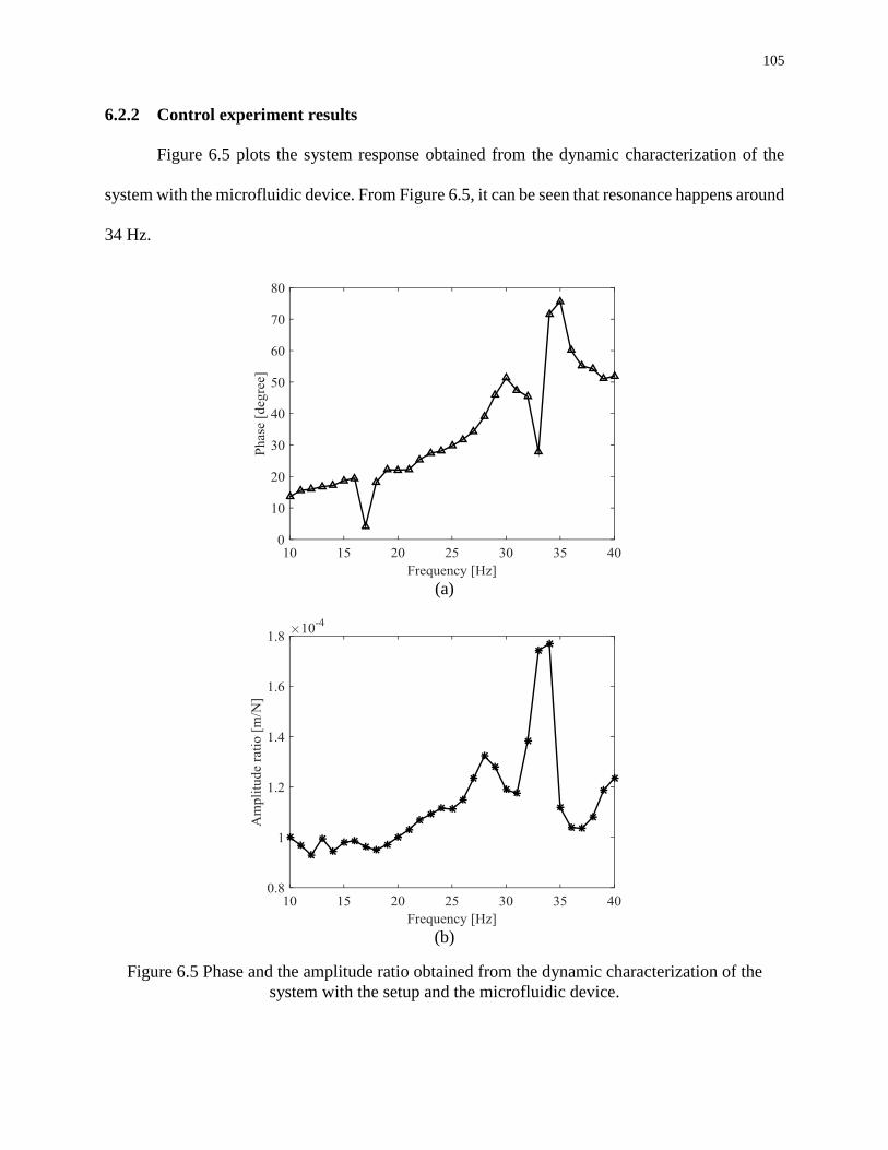
105
6.2.2 Control experiment results
Figure 6.5 plots the system response obtained from the dynamic characterization of the
system with the microfluidic device. From Figure 6.5, it can be seen that resonance happens around
34 Hz.
(a)
(b)
Figure 6.5 Phase and the amplitude ratio obtained from the dynamic characterization of the
system with the setup and the microfluidic device.
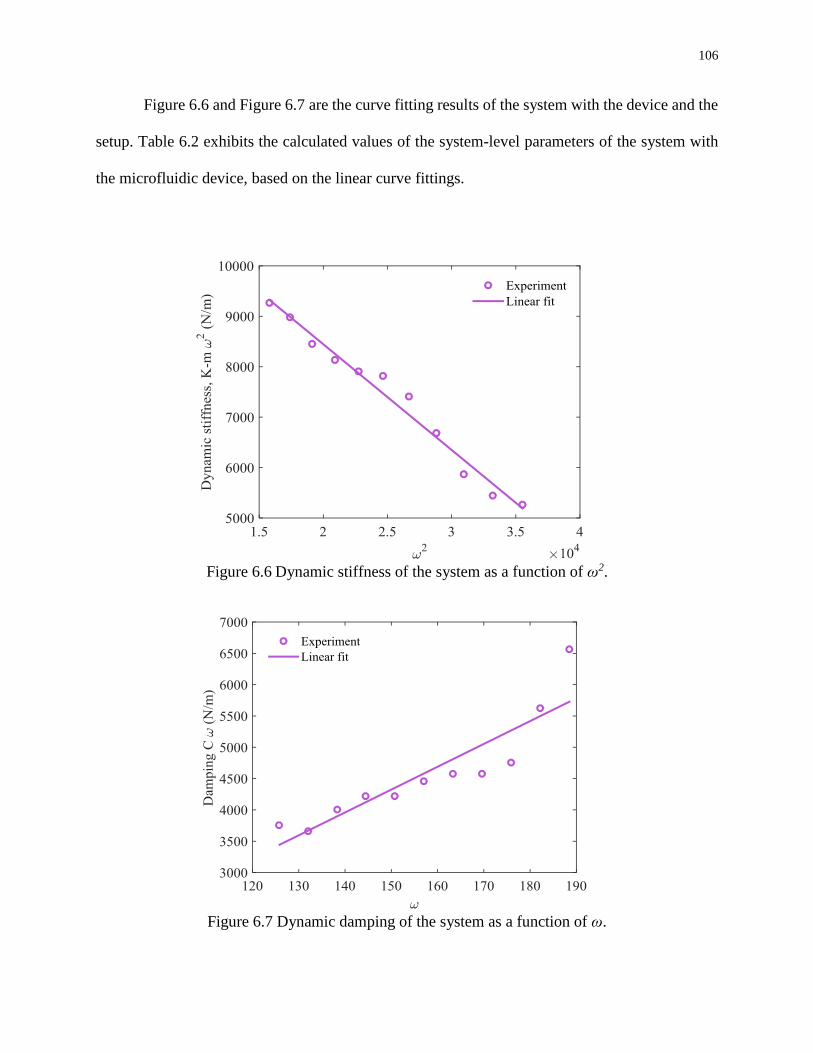
106
Figure 6.6 and Figure 6.7 are the curve fitting results of the system with the device and the
setup. Table 6.2 exhibits the calculated values of the system-level parameters of the system with
the microfluidic device, based on the linear curve fittings.
Figure 6.6 Dynamic stiffness of the system as a function of ω2.
Figure 6.7 Dynamic damping of the system as a function of ω.

107
Table 6.2 System-level parameters of the dynamic system with the microfluidic device and the
setup, based on the linear curve fitting.
KD (N/m) 12637
MD (kg) 0.2096
CD (Ns/m) 36.457
Based on these values, the natural frequency, damping ratio, damped frequency, and the
quality factor of the system are calculated, and these values are listed in Table 6.3.
Table 6.3 System-level properties of the dynamic system.
System level
properties
values
f0 (Hz) 39.04
ζ 0.354
fd (Hz) 34.14
Q 1.41
6.2.3 Measurement results of the samples
After extracting the system level parameters of the dynamic system with the device alone,
the measurement results with a piece of test sample in the dynamic system are also achieved.
Figure 6.8 plots the measurement results of the Dragon Skin 10 sample. As can be seen from both
the phase and compliance diagrams, the resonance happens at around 23 Hz. Compared with the
damped resonance value obtained previously in the control experiment without the sample, which
is around 34 Hz, the resonance frequency decreased. The decrease is caused by the change of
contact stiffness, which further contains information of the mechanical property of the unknown
sample. In Figure 6.8 (a), the phase shift obtained from the experimental data at around 40 Hz
exceeds 180 °. It is possibly caused by a time delay during the sequential data acquisition process.
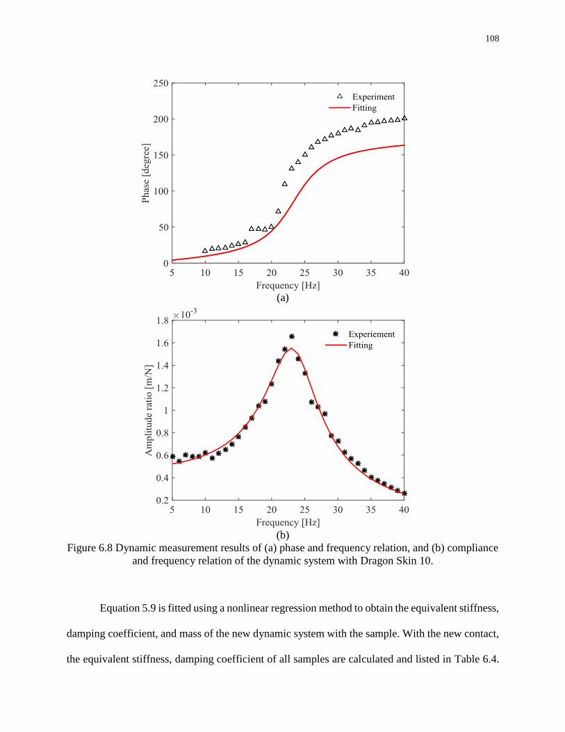
108
(a)
(b)
Figure 6.8 Dynamic measurement results of (a) phase and frequency relation, and (b) compliance
and frequency relation of the dynamic system with Dragon Skin 10.
Equation 5.9 is fitted using a nonlinear regression method to obtain the equivalent stiffness,
damping coefficient, and mass of the new dynamic system with the sample. With the new contact,
the equivalent stiffness, damping coefficient of all samples are calculated and listed in Table 6.4.
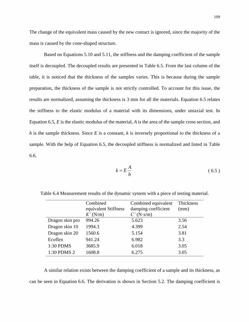
109
The change of the equivalent mass caused by the new contact is ignored, since the majority of the
mass is caused by the cone-shaped structure.
Based on Equations 5.10 and 5.11, the stiffness and the damping coefficient of the sample
itself is decoupled. The decoupled results are presented in Table 6.5. From the last column of the
table, it is noticed that the thickness of the samples varies. This is because during the sample
preparation, the thickness of the sample is not strictly controlled. To account for this issue, the
results are normalized, assuming the thickness is 3 mm for all the materials. Equation 6.5 relates
the stiffness to the elastic modulus of a material with its dimensions, under uniaxial test. In
Equation 6.5, E is the elastic modulus of the material, A is the area of the sample cross section, and
h is the sample thickness. Since E is a constant, k is inversely proportional to the thickness of a
sample. With the help of Equation 6.5, the decoupled stiffness is normalized and listed in Table
6.6.
Ak E
h ( 6.5 )
Table 6.4 Measurement results of the dynamic system with a piece of testing material.
Combined
equivalent Stiffness
K’ (N/m)
Combined equivalent
damping coefficient
C’ (N·s/m)
Thickness
(mm)
Dragon skin pro 994.26 5.623 3.56
Dragon skin 10 1994.3 4.399 2.54
Dragon skin 20 1560.6 5.154 3.81
Ecoflex 941.24 6.982 3.3
1:30 PDMS 3685.9 6.018 3.05
1:30 PDMS 2 1608.8 6.275 3.05
A similar relation exists between the damping coefficient of a sample and its thickness, as
can be seen in Equation 6.6. The derivation is shown in Section 5.2. The damping coefficient is
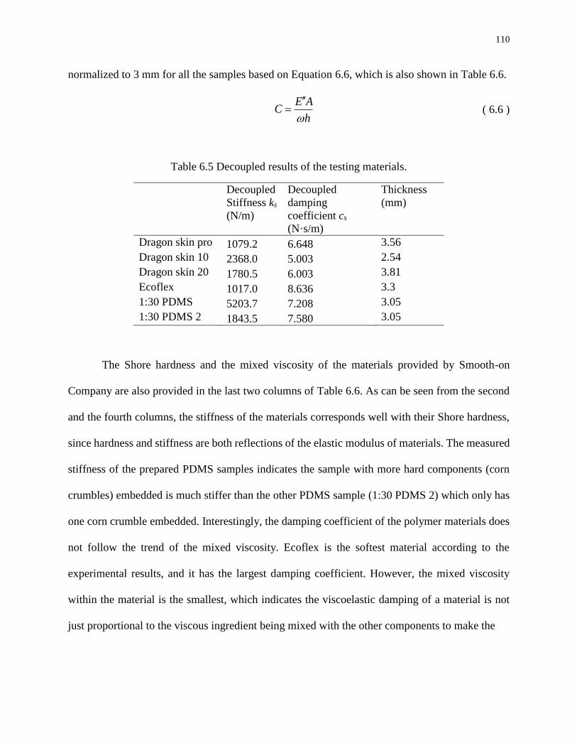
110
normalized to 3 mm for all the samples based on Equation 6.6, which is also shown in Table 6.6.
E AC
h
( 6.6 )
Table 6.5 Decoupled results of the testing materials.
Decoupled
Stiffness ks
(N/m)
Decoupled
damping
coefficient cs
(N·s/m)
Thickness
(mm)
Dragon skin pro 1079.2 6.648 3.56
Dragon skin 10 2368.0 5.003 2.54
Dragon skin 20 1780.5 6.003 3.81
Ecoflex 1017.0 8.636 3.3
1:30 PDMS 5203.7 7.208 3.05
1:30 PDMS 2 1843.5 7.580 3.05
The Shore hardness and the mixed viscosity of the materials provided by Smooth-on
Company are also provided in the last two columns of Table 6.6. As can be seen from the second
and the fourth columns, the stiffness of the materials corresponds well with their Shore hardness,
since hardness and stiffness are both reflections of the elastic modulus of materials. The measured
stiffness of the prepared PDMS samples indicates the sample with more hard components (corn
crumbles) embedded is much stiffer than the other PDMS sample (1:30 PDMS 2) which only has
one corn crumble embedded. Interestingly, the damping coefficient of the polymer materials does
not follow the trend of the mixed viscosity. Ecoflex is the softest material according to the
experimental results, and it has the largest damping coefficient. However, the mixed viscosity
within the material is the smallest, which indicates the viscoelastic damping of a material is not
just proportional to the viscous ingredient being mixed with the other components to make the
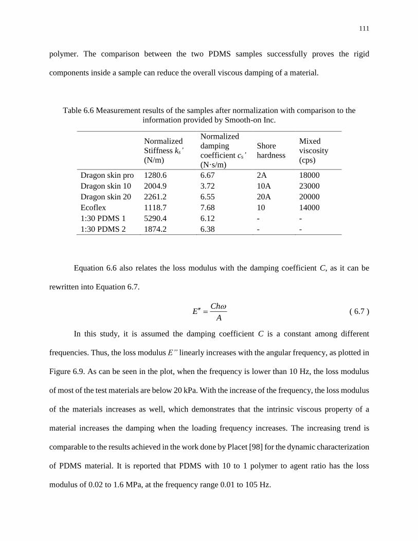
111
polymer. The comparison between the two PDMS samples successfully proves the rigid
components inside a sample can reduce the overall viscous damping of a material.
Table 6.6 Measurement results of the samples after normalization with comparison to the
information provided by Smooth-on Inc.
Normalized
Stiffness ks’
(N/m)
Normalized
damping
coefficient cs’
(N·s/m)
Shore
hardness
Mixed
viscosity
(cps)
Dragon skin pro 1280.6 6.67 2A 18000
Dragon skin 10 2004.9 3.72 10A 23000
Dragon skin 20 2261.2 6.55 20A 20000
Ecoflex 1118.7 7.68 10 14000
1:30 PDMS 1 5290.4 6.12 - -
1:30 PDMS 2 1874.2 6.38 - -
Equation 6.6 also relates the loss modulus with the damping coefficient C, as it can be
rewritten into Equation 6.7.
A
ChE
( 6.7 )
In this study, it is assumed the damping coefficient C is a constant among different
frequencies. Thus, the loss modulus E” linearly increases with the angular frequency, as plotted in
Figure 6.9. As can be seen in the plot, when the frequency is lower than 10 Hz, the loss modulus
of most of the test materials are below 20 kPa. With the increase of the frequency, the loss modulus
of the materials increases as well, which demonstrates that the intrinsic viscous property of a
material increases the damping when the loading frequency increases. The increasing trend is
comparable to the results achieved in the work done by Placet [98] for the dynamic characterization
of PDMS material. It is reported that PDMS with 10 to 1 polymer to agent ratio has the loss
modulus of 0.02 to 1.6 MPa, at the frequency range 0.01 to 105 Hz.
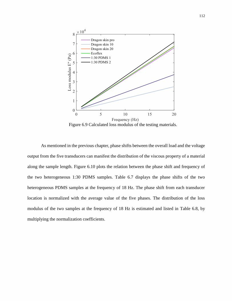
112
Figure 6.9 Calculated loss modulus of the testing materials.
As mentioned in the previous chapter, phase shifts between the overall load and the voltage
output from the five transducers can manifest the distribution of the viscous property of a material
along the sample length. Figure 6.10 plots the relation between the phase shift and frequency of
the two heterogeneous 1:30 PDMS samples. Table 6.7 displays the phase shifts of the two
heterogeneous PDMS samples at the frequency of 18 Hz. The phase shift from each transducer
location is normalized with the average value of the five phases. The distribution of the loss
modulus of the two samples at the frequency of 18 Hz is estimated and listed in Table 6.8, by
multiplying the normalization coefficients.
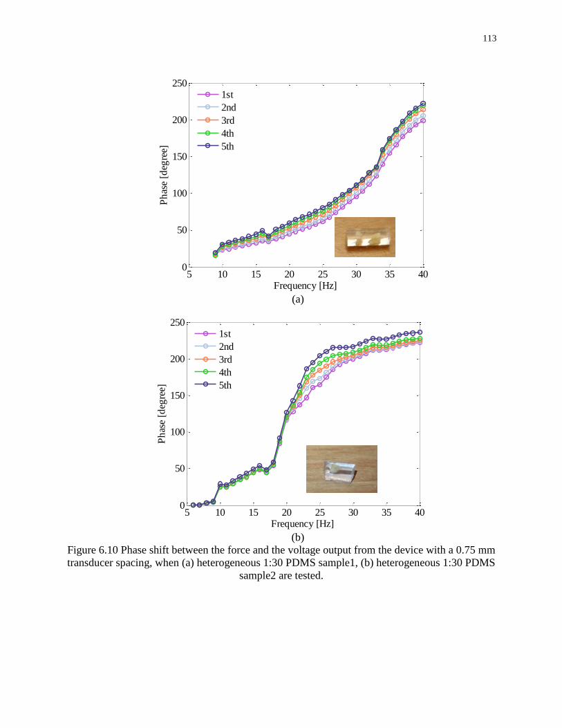
113
(a)
(b)
Figure 6.10 Phase shift between the force and the voltage output from the device with a 0.75 mm
transducer spacing, when (a) heterogeneous 1:30 PDMS sample1, (b) heterogeneous 1:30 PDMS
sample2 are tested.
5 10 15 20 25 30 35 400
50
100
150
200
250
Frequency [Hz]
Ph
ase
[deg
ree]
1st
2nd
3rd
4th
5th
5 10 15 20 25 30 35 400
50
100
150
200
250
Frequency [Hz]
Ph
ase
[deg
ree]
1st
2nd
3rd
4th
5th
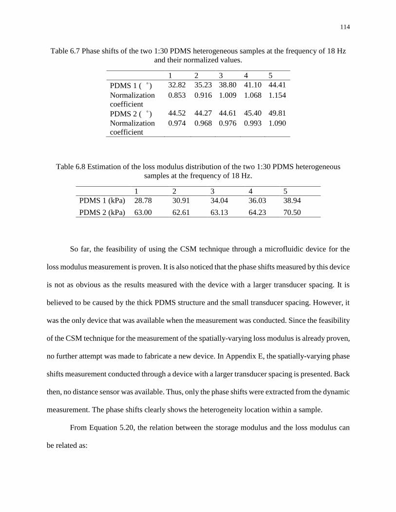
114
Table 6.7 Phase shifts of the two 1:30 PDMS heterogeneous samples at the frequency of 18 Hz
and their normalized values.
1 2 3 4 5
PDMS 1 (︒) 32.82 35.23 38.80 41.10 44.41
Normalization
coefficient
0.853 0.916 1.009 1.068 1.154
PDMS 2 (︒) 44.52 44.27 44.61 45.40 49.81
Normalization
coefficient
0.974 0.968 0.976 0.993 1.090
Table 6.8 Estimation of the loss modulus distribution of the two 1:30 PDMS heterogeneous
samples at the frequency of 18 Hz.
1 2 3 4 5
PDMS 1 (kPa) 28.78 30.91 34.04 36.03 38.94
PDMS 2 (kPa) 63.00 62.61 63.13 64.23 70.50
So far, the feasibility of using the CSM technique through a microfluidic device for the
loss modulus measurement is proven. It is also noticed that the phase shifts measured by this device
is not as obvious as the results measured with the device with a larger transducer spacing. It is
believed to be caused by the thick PDMS structure and the small transducer spacing. However, it
was the only device that was available when the measurement was conducted. Since the feasibility
of the CSM technique for the measurement of the spatially-varying loss modulus is already proven,
no further attempt was made to fabricate a new device. In Appendix E, the spatially-varying phase
shifts measurement conducted through a device with a larger transducer spacing is presented. Back
then, no distance sensor was available. Thus, only the phase shifts were extracted from the dynamic
measurement. The phase shifts clearly shows the heterogeneity location within a sample.
From Equation 5.20, the relation between the storage modulus and the loss modulus can
be related as:
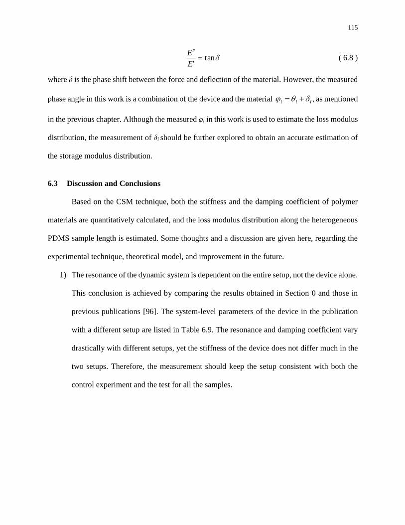
115
tan
E
E ( 6.8 )
where δ is the phase shift between the force and deflection of the material. However, the measured
phase angle in this work is a combination of the device and the material iii , as mentioned
in the previous chapter. Although the measured φi in this work is used to estimate the loss modulus
distribution, the measurement of δi should be further explored to obtain an accurate estimation of
the storage modulus distribution.
6.3 Discussion and Conclusions
Based on the CSM technique, both the stiffness and the damping coefficient of polymer
materials are quantitatively calculated, and the loss modulus distribution along the heterogeneous
PDMS sample length is estimated. Some thoughts and a discussion are given here, regarding the
experimental technique, theoretical model, and improvement in the future.
1) The resonance of the dynamic system is dependent on the entire setup, not the device alone.
This conclusion is achieved by comparing the results obtained in Section 0 and those in
previous publications [96]. The system-level parameters of the device in the publication
with a different setup are listed in Table 6.9. The resonance and damping coefficient vary
drastically with different setups, yet the stiffness of the device does not differ much in the
two setups. Therefore, the measurement should keep the setup consistent with both the
control experiment and the test for all the samples.
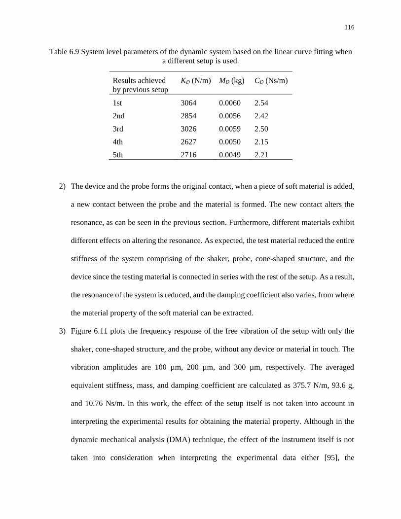
116
Table 6.9 System level parameters of the dynamic system based on the linear curve fitting when
a different setup is used.
Results achieved
by previous setup
KD (N/m) MD (kg) CD (Ns/m)
1st 3064 0.0060 2.54
2nd 2854 0.0056 2.42
3rd 3026 0.0059 2.50
4th 2627 0.0050 2.15
5th 2716 0.0049 2.21
2) The device and the probe forms the original contact, when a piece of soft material is added,
a new contact between the probe and the material is formed. The new contact alters the
resonance, as can be seen in the previous section. Furthermore, different materials exhibit
different effects on altering the resonance. As expected, the test material reduced the entire
stiffness of the system comprising of the shaker, probe, cone-shaped structure, and the
device since the testing material is connected in series with the rest of the setup. As a result,
the resonance of the system is reduced, and the damping coefficient also varies, from where
the material property of the soft material can be extracted.
3) Figure 6.11 plots the frequency response of the free vibration of the setup with only the
shaker, cone-shaped structure, and the probe, without any device or material in touch. The
vibration amplitudes are 100 µm, 200 µm, and 300 µm, respectively. The averaged
equivalent stiffness, mass, and damping coefficient are calculated as 375.7 N/m, 93.6 g,
and 10.76 Ns/m. In this work, the effect of the setup itself is not taken into account in
interpreting the experimental results for obtaining the material property. Although in the
dynamic mechanical analysis (DMA) technique, the effect of the instrument itself is not
taken into consideration when interpreting the experimental data either [95], the
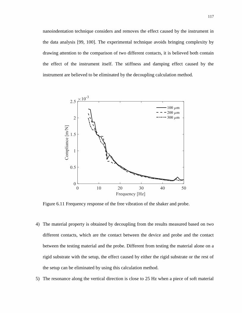
117
nanoindentation technique considers and removes the effect caused by the instrument in
the data analysis [99, 100]. The experimental technique avoids bringing complexity by
drawing attention to the comparison of two different contacts, it is believed both contain
the effect of the instrument itself. The stiffness and damping effect caused by the
instrument are believed to be eliminated by the decoupling calculation method.
Figure 6.11 Frequency response of the free vibration of the shaker and probe.
4) The material property is obtained by decoupling from the results measured based on two
different contacts, which are the contact between the device and probe and the contact
between the testing material and the probe. Different from testing the material alone on a
rigid substrate with the setup, the effect caused by either the rigid substrate or the rest of
the setup can be eliminated by using this calculation method.
5) The resonance along the vertical direction is close to 25 Hz when a piece of soft material
118
is under testing with the current setup. This value is lower than it is expected, since the
frequency of the mechanical noise in the environment is around the value. To avoid this
situation, the setup should be designed more rigidly and with less weight to increase its
resonance in the future.
6) The formula used to achieve the loss modulus and to normalize the results is based on the
assumption of uniaxial uniform loading. The actual loading condition differs from the
assumption, which requires a more accurate theoretical model to relate the relations.
7) Figure 6.6 shows a good linear relation between the dynamic stiffness and the square of
angular frequency, however Figure 6.7 does not show a good linear fitting. It can be
attributed to fact that K and M of the system are constants, however, C actually varies
among different frequencies. Instead of assuming C is a constant in this work, a function
of frequency should be used to express C in the future.
Overall, along with the previous chapter, this chapter presents the implementation of the
CSM technique for the measurement of the spatially-varying loss modulus of soft materials. This
is the first attempt so far to measure this property using one single device through the harmonic
test. The obtained stiffness of the homogeneous samples matches well with the hardness provided
by the manufacturer. The obtained loss modulus of PDMS samples is within the range provided
by other researchers.

119
CHAPTER 7
CONCLUSIONS AND FUTURE WORK
In this chapter, the highlights and conclusive remarks of this dissertation are presented, and
recommendations for the future work are proposed based on the current achievement.
7.1 Discussion
There are several drawbacks associated with the current device and the experimental
technique.
1. Cross talk between sensing units exists in the current microfluidic device.
2. Several assumptions are used in the formula deduction of this work, such as the small strain
assumption. Ideally, the strain should be smaller than 10% under this assumption.
However, the actual strain applied may exceed the upper limit.
3. For now, the in vivo test still hasn’t been achieved. Soft materials were cut into a thin slice,
and put on top of the device for further measurement. As a result, for biological tissues, the
measured material properties may be different from tissues in a living state.
4. The current experimental technique still relies on a controlled displacement applied to the
soft material sample through an external instrument, which limits the application inside the
lab.
5. The voltage drift issue is investigated but still remains unsolvable.
7.2 Conclusions
This work focuses on the application of a microfluidic device for distributed-load detection.
The main achievement of this work includes the following aspects.
120
1. A detailed input and output relation of one sensing segment of the microfluidic device is
presented. The controlled input to the device is usually an indentation depth applied by a
probe. The relationship between the displacement and the output voltage of the device is
studied both theoretically and numerically. The linear relation between the prescribed
indentation depth and the reaction force and the linear relation between the prescribed
indentation depth and the output voltage from the numerical analysis is consistent with the
results obtained from the characterization experiment. Based on these relations, device
design and optimization can be carried out.
2. For the first time, the technical issues associated with the device and the experimental
technique, such as voltage drift and probe misalignment issues are thoroughly studied. The
voltage drift issue is experimentally explored, and the misalignment issue is explained in
detail using numerical simulation.
3. A mathematical model to relate the force and indentation depth of a rigid cylindrical probe
pressing upon a flat piece of material with finite thickness is proposed. Thus, the foundation
of using the microfluidic device to measure the elastic modulus of a flat piece of soft
material through a cylindrical probe and a load cell is established.
4. Most importantly, this work proved the capability of using the microfluidic device to
distinguish heterogeneity within a piece of soft material and quantitatively obtain its
spatially-varying viscoelastic properties along the sample length from the indentation and
dynamic tests, respectively.
The main contribution of this work is that it lays down the foundation for applying a
microfluidic device to achieve the CSM of the viscoelastic properties of soft materials. This work
shows the simplicity in the device fabrication, and the efficiency in the measurement. The samples

121
used in this work are polymers, including customized PDMS samples with heterogeneity and
standard commercialized polymer samples that are widely used to mimic biological samples or
build polymer-based sensors.
7.3 Future Work
1. Number of transducers
The devices employed in this work only involves five sensing segments for simplicity.
Devices with sensing segment arrays should be explored to increase the number of
transducers, so that it can measure the viscoelastic properties of soft materials at more
locations within one measurement.
2. Crosstalk or coupling should be experimentally explored
In this work, weak crosstalk or coupling from both mechanical and electrical aspects is
assumed. It is necessary to explore the crosstalk or coupling in the future for a better
calibration of the device.
3. Improvement of the experimental setup
In the experimental setup exhibited in Chapter 6, the cone-shaped structure is connected
below the load cell, which brings complexity to the vibration system. In the future work,
structure with less weight should be designed and incorporated in the vibration system for
reflecting the laser beam from the distance sensor.
4. Device design and optimization
In Chapter 2, the input and output relation of the device is established numerically. Based
on the simulation, device design and optimization through building a surrogate model and
applying optimization algorithm becomes achievable. The measurement range of the

122
device should be quantified. Improvement should be made to increase the device sensitivity
and the output linearity.
5. Flexible substrate
The current design of the microfluidic device has a rigid substrate, which helps maintain
its mechanical stability, yet this limits its application, especially when PDMS is a flexible,
biocompatible material. A device with a flexible substrate should be explored for obtaining
a bendable device, which can be further attached to surfaces with curvature.
6. Better wire connections and packaging
The current device adopted a wire bonding technique from MEMS technology to make the
electrical connections to a PCB board which further connects to the circuits. The bonding
wire is thin and vulnerable; a small mechanical impact or accidental touch would cause a
disconnection, which is inconvenient even for an in vitro test, and makes an in vivo test
even more difficult. To solve this problem, a better solution for connections between the
device and the rest of the circuit is very necessary.
7. Apply the methodology to biological tissues
The data collected in this work are based on surrogates that are commonly used to mimic
biological tissues, such as PDMS, dragon skin, and agarose gels. The mechanical property
of biological tissues, such as cartilage and blood vessels is of utmost research interest and
the initial design interest of the microfluidic device. Since the capability of the CSM of the
viscoelastic properties of soft materials is already proven by this work, future work should
focus on applying this technique to biological samples and relating the obtained results to
pathological observations. Improve the load/displacement actuation mechanism to achieve
integrated design. As mentioned in Section 7.1, the external mechanical excitation is added
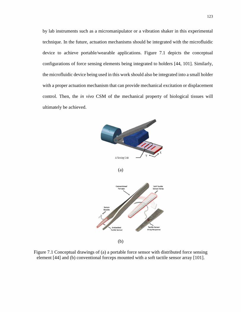
123
by lab instruments such as a micromanipulator or a vibration shaker in this experimental
technique. In the future, actuation mechanisms should be integrated with the microfluidic
device to achieve portable/wearable applications. Figure 7.1 depicts the conceptual
configurations of force sensing elements being integrated to holders [44, 101]. Similarly,
the microfluidic device being used in this work should also be integrated into a small holder
with a proper actuation mechanism that can provide mechanical excitation or displacement
control. Then, the in vivo CSM of the mechanical property of biological tissues will
ultimately be achieved.
(a)
(b)
Figure 7.1 Conceptual drawings of (a) a portable force sensor with distributed force sensing
element [44] and (b) conventional forceps mounted with a soft tactile sensor array [101].

124
REFERENCES
[1] Y. Menguc, Y.-L. Park, E. Martinez-Villalpando, P. Aubin, M. Zisook, L. Stirling, et al.,
"Soft wearable motion sensing suit for lower limb biomechanics measurements," in
Robotics and Automation (ICRA), 2013 IEEE International Conference on, 2013, pp.
5309-5316.
[2] M. Puttock and E. Thwaite, Elastic compression of spheres and cylinders at point and
line contact: Commonwealth Scientific and Industrial Research Organization Melbourne,
VIC, Australia, 1969.
[3] Y. Menguc, Y. L. Park, H. Pei, D. Vogt, P. M. Aubin, E. Winchell, et al., "Wearable soft
sensing suit for human gait measurement," International Journal of Robotics Research,
vol. 33, pp. 1748-1764, Dec 2014.
[4] P. Du, C. Cheng, H. B. Lu, and X. Zhang, "Investigation of Cellular Contraction Forces
in the Frequency Domain Using a PDMS Micropillar-Based Force Transducer," Journal
of Microelectromechanical Systems, vol. 22, pp. 44-53, Feb 2013.
[5] S. Zorner, M. Kaltenbacher, R. Lerch, A. Sutor, and M. Dollinger, "Measurement of the
elasticity modulus of soft tissues," Journal of Biomechanics, vol. 43, pp. 1540-1545, May
28 2010.
[6] R. Akhtar, M. J. Sherratt, J. K. Cruickshank, and B. Derby, "Characterizing the elastic
properties of tissues," Materials Today, vol. 14, pp. 96-105, Mar 2011.
[7] C.-L. Chen, E. Lopez, P. Makaram, S. Selvarasah, A. Busnaina, Y.-J. Jung, et al.,
"Fabrication and evaluation of carbon nanotube-parylene functional composite-films," in
Solid-State Sensors, Actuators and Microsystems Conference, 2007. TRANSDUCERS
2007. International, 2007, pp. 1019-1022.
[8] I. D. Johnston, D. K. McCluskey, C. K. L. Tan, and M. C. Tracey, "Mechanical
characterization of bulk Sylgard 184 for microfluidics and microengineering," Journal of
Micromechanics and Microengineering, vol. 24, Mar 2014.
[9] T. K. Kim, J. K. Kim, and O. C. Jeong, "Measurement of nonlinear mechanical properties
of PDMS elastomer," Microelectronic Engineering, vol. 88, pp. 1982-1985, Aug 2011.
[10] F. Schneider, J. Draheirn, R. Kamberger, and U. Wallrabe, "Process and material
properties of polydimethylsiloxane (PDMS) for Optical MEMS," Sensors and Actuators
a-Physical, vol. 151, pp. 95-99, Apr 29 2009.
[11] F. M. Yaul, V. Bulovic, and J. H. Lang, "A Flexible Underwater Pressure Sensor Array
Using a Conductive Elastomer Strain Gauge," Journal of Microelectromechanical
Systems, vol. 21, pp. 897-907, Aug 2012.
[12] G. Y. H. Lee and C. T. Lim, "Biomechanics approaches to studying human diseases,"
Trends in Biotechnology, vol. 25, pp. 111-118, Mar 2007.
[13] E. G. Lakatta and D. Levy, "Arterial and cardiac aging: Major shareholders in
cardiovascular disease enterprises Part I: Aging arteries: A "set up" for vascular disease,"
Circulation, vol. 107, pp. 139-146, Jan 7 2003.
[14] S. Suresh, J. Spatz, J. P. Mills, A. Micoulet, M. Dao, C. T. Lim, et al., "Connections
between single-cell biomechanics and human disease states: gastrointestinal cancer and
malaria," Acta Biomaterialia, vol. 1, pp. 15-30, Jan 2005.
[15] C. T. McKee, J. A. Last, P. Russell, and C. J. Murphy, "Indentation Versus Tensile
Measurements of Young's Modulus for Soft Biological Tissues," Tissue Engineering Part
B-Reviews, vol. 17, pp. 155-164, Jun 2011.
125
[16] M. M. Brandao, A. Fontes, M. L. Barjas-Castro, L. C. Barbosa, F. F. Costa, C. L. Cesar,
et al., "Optical tweezers for measuring red blood cell elasticity: application to the study
of drug response in sickle cell disease," European Journal of Haematology, vol. 70, pp.
207-211, Apr 2003.
[17] C. L. Ives, S. G. Eskin, and L. V. Mcintire, "Mechanical Effects on Endothelial-Cell
Morphology - Invitro Assessment," In Vitro Cellular & Developmental Biology, vol. 22,
pp. 500-507, Sep 1986.
[18] K. L. Troyer, D. J. Estep, and C. M. Puttlitz, "Viscoelastic effects during loading play an
integral role in soft tissue mechanics," Acta biomaterialia, vol. 8, pp. 234-243, 2012.
[19] L. M. Rebelo, J. S. de Sousa, J. Mendes, and M. Radmacher, "Comparison of the
viscoelastic properties of cells from different kidney cancer phenotypes measured with
atomic force microscopy," Nanotechnology, vol. 24, Feb 8 2013.
[20] H. Suzuki, M. Suga, K. Fujisaki, I. Kajiwara, G. Nakamura, K. Yoshikawa, et al.,
"Viscoelastic Properties of Gel Material and Soft Tissue Measured by MRE (Magnetic
Resonance Elastography) Using Micro MRE," in The 15th International Conference on
Biomedical Engineering, 2014, pp. 156-159.
[21] E. Lehmann, "Noninvasive measurements of aortic stiffness: methodological
considerations," Pathologie-biologie, vol. 47, pp. 716-730, 1999.
[22] R. Muthupillai, D. Lomas, P. Rossman, J. Greenleaf, A. Manduca, and R. Ehman,
"Magnetic resonance elastography by direct visualization of propagating acoustic strain
waves," Science, vol. 269, pp. 1854-1857, 1995.
[23] S. Chen, M. W. Urban, C. Pislaru, R. Kinnick, Y. Zheng, A. Yao, et al., "Shearwave
dispersion ultrasound vibrometry (SDUV) for measuring tissue elasticity and viscosity,"
Ultrasonics, Ferroelectrics, and Frequency Control, IEEE Transactions on, vol. 56, pp.
55-62, 2009.
[24] E. M. Darling, R. E. Wilusz, M. P. Bolognesi, S. Zauscher, and F. Guilak, "Spatial
Mapping of the Biomechanical Properties of the Pericellular Matrix of Articular Cartilage
Measured In Situ via Atomic Force Microscopy," Biophysical Journal, vol. 98, pp. 2848-
2856, Jun 16 2010.
[25] E. K. Dimitriadis, F. Horkay, J. Maresca, B. Kachar, and R. S. Chadwick, "Determination
of elastic moduli of thin layers of soft material using the atomic force microscope,"
Biophysical Journal, vol. 82, pp. 2798-2810, May 2002.
[26] O. Franke, M. Goken, M. A. Meyers, K. Durst, and A. M. Hodge, "Dynamic
nanoindentation of articular porcine cartilage," Materials Science & Engineering C-
Materials for Biological Applications, vol. 31, pp. 789-795, May 10 2011.
[27] L. Han, E. H. Frank, J. J. Greene, H. Y. Lee, H. H. K. Hung, A. J. Grodzinsky, et al.,
"Time-Dependent Nanomechanics of Cartilage," Biophysical Journal, vol. 100, pp. 1846-
1854, Apr 6 2011.
[28] D. Hoffman, "Measuring the elastic modulus of polymers using the atomic force
microscope," Master's Master's Thesis, Michigan Technological University, 2010.
[29] T. A. Krouskop, T. M. Wheeler, F. Kallel, B. S. Garra, and T. Hall, "Elastic moduli of
breast and prostate tissues under compression," Ultrasonic Imaging, vol. 20, pp. 260-274,
Oct 1998.
[30] D. C. Lin and F. Horkay, "Nanomechanics of polymer gels and biological tissues: A
critical review of analytical approaches in the Hertzian regime and beyond," Soft Matter,
vol. 4, pp. 669-682, 2008.

126
[31] V. T. Nayar, J. D. Weiland, C. S. Nelson, and A. M. Hodge, "Elastic and viscoelastic
characterization of agar," Journal of the Mechanical Behavior of Biomedical Materials,
vol. 7, pp. 60-68, Mar 2012.
[32] G. Scarcelli and S. H. Yun, "Confocal Brillouin microscopy for three-dimensional
mechanical imaging," Nature Photonics, vol. 2, pp. 39-43, Jan 2008.
[33] Y. J. Kim, L. J. Bonassar, and A. J. Grodzinsky, "The Role of Cartilage Streaming
Potential, Fluid-Flow and Pressure in the Stimulation of Chondrocyte Biosynthesis
during Dynamic Compression," Journal of Biomechanics, vol. 28, pp. 1055-1066, Sep
1995.
[34] M. R. Buckley, L. J. Bonassar, and I. Cohen, "Localization of Viscous Behavior and
Shear Energy Dissipation in Articular Cartilage Under Dynamic Shear Loading," Journal
of Biomechanical Engineering-Transactions of the Asme, vol. 135, Mar 2013.
[35] M. R. Buckley, J. P. Gleghorn, L. J. Bonassar, and I. Cohen, "Mapping the depth
dependence of shear properties in articular cartilage," Journal of Biomechanics, vol. 41,
pp. 2430-2437, Aug 7 2008.
[36] Z. Wang, "Polydimethylsiloxane mechanical properties measured by macroscopic
compression and nanoindentation techniques," 2011.
[37] M. A. McLeod, R. E. Wilusz, and F. Guilak, "Depth-dependent anisotropy of the
micromechanical properties of the extracellular and pericellular matrices of articular
cartilage evaluated via atomic force microscopy," Journal of Biomechanics, vol. 46, pp.
586-592, Feb 1 2013.
[38] C. Florea, M. Dreucean, M. S. Laasanen, and A. Halvari, "Determination of young's
modulus using AFM nanoindentation. Applications on bone structures," in E-Health and
Bioengineering Conference (EHB), 2011, 2011, pp. 1-4.
[39] Wikipedia, "Atomic force microscopy," 2013.
[40] S. K. Kaliappan, "Characterization of physical properties of polymers using AFM force-
distance curves," 2007.
[41] T. Neumann, "Determining the elastic modulus of biological samples using atomic force
microscopy," JPK Instruments Application Report, pp. 1-9, 2008.
[42] N. Gavara and R. S. Chadwick, "Determination of the elastic moduli of thin samples and
adherent cells using conical atomic force microscope tips," Nature Nanotechnology, vol.
7, pp. 733-736, Nov 2012.
[43] W. Y. Zhang, M. Gnerlich, J. J. Paly, Y. H. Sun, G. S. Jing, A. Voloshin, et al., "A
polymer V-shaped electrothermal actuator array for biological applications," Journal of
Micromechanics and Microengineering, vol. 18, Jul 2008.
[44] S. Sokhanvar, M. Packirisamy, and J. Dargahi, "MEMS Endoscopic Tactile Sensor:
Toward In-Situ and In-Vivo and Tissue Softness Characterization," Ieee Sensors Journal,
vol. 9, pp. 1679-1687, Dec 2009.
[45] A. Atieh, "Design, Modeling, Fabrication and Testing of a Piezoresistive-Based Tactile
Sensor for Minimally Invasive Surgery Applications," Masters, Mechanical Engineering,
Concordia University, 2012.
[46] P. R. Dhar and J. W. Zu, "Design of a resonator device for in vivo measurement of
regional tissue viscoelasticity," Sensors and Actuators a-Physical, vol. 133, pp. 45-54,
Jan 8 2007.

127
[47] D. N. Hohne, J. G. Younger, and M. J. Solomon, "Flexible Microfluidic Device for
Mechanical Property Characterization of Soft Viscoelastic Solids Such as Bacterial
Biofilms," Langmuir, vol. 25, pp. 7743-7751, Jul 7 2009.
[48] E. A. Corbin, L. J. Millet, J. H. Pikul, C. L. Johnson, J. G. Georgiadis, W. P. King, et al.,
"Micromechanical properties of hydrogels measured with MEMS resonant sensors,"
Biomedical Microdevices, vol. 15, pp. 311-319, Apr 2013.
[49] K. Kim, X. Y. Liu, Y. Zhang, J. Cheng, X. Yu Wu, and Y. Sun, "Elastic and viscoelastic
characterization of microcapsules for drug delivery using a force-feedback MEMS
microgripper," Biomedical Microdevices, vol. 11, pp. 421-427, Apr 2009.
[50] S. J. Lee, M. A. King, J. Sun, H. K. Xie, G. Subhash, and M. Sarntinoranont,
"Measurement of viscoelastic properties in multiple anatomical regions of acute rat brain
tissue slices," Journal of the Mechanical Behavior of Biomedical Materials, vol. 29, pp.
213-224, Jan 2014.
[51] Y. Tatara, "Large Deformations of a Rubber Sphere under Diametral Compression .1.
Theoretical-Analysis of Press Approach, Contact Radius and Lateral Extension," Jsme
International Journal Series a-Mechanics and Material Engineering, vol. 36, pp. 190-
196, Apr 1993.
[52] P. Peng, "Novel MEMS Tactile Sensors for In-Vivo Tissue Characterization
Measurements," UNIVERSITY OF MINNESOTA, 2011.
[53] Z. L. L. Shen, H. Kahn, R. Ballarin, and S. J. Eppell, "Viscoelastic Properties of Isolated
Collagen Fibrils," Biophysical Journal, vol. 100, pp. 3008-3015, Jun 22 2011.
[54] C. Tzikang, "Determining a Prony series for a viscoelastic material from time varying
strain data," 2000.
[55] M. Radmacher, "Measuring the elastic properties of biological samples with the AFM,"
Engineering in Medicine and Biology Magazine, IEEE, vol. 16, pp. 47-57, 1997.
[56] C. A. Gutierrez and E. Meng, "Impedance-Based Force Transduction Within Fluid-Filled
Parylene Microstructures," Journal of Microelectromechanical Systems, vol. 20, pp.
1098-1108, Oct 2011.
[57] H. J. Pandya, K. Park, and J. P. Desai, "Design and fabrication of a flexible MEMS-based
electro-mechanical sensor array for breast cancer diagnosis," Journal of Micromechanics
and Microengineering, vol. 25, Jul 2015.
[58] P. Peng and R. Rajamani, "Handheld Microtactile Sensor for Elasticity Measurement,"
Ieee Sensors Journal, vol. 11, pp. 1935-1942, Sep 2011.
[59] R. Ahmadi, M. Packirisamy, J. Dargahi, and R. Cecere, "Discretely Loaded Beam-Type
Optical Fiber Tactile Sensor for Tissue Manipulation and Palpation in Minimally
Invasive Robotic Surgery," Ieee Sensors Journal, vol. 12, pp. 22-32, Jan 2012.
[60] P. Cheng, W. Gu, J. Shen, A. Ghosh, A. Beskok, and Z. Hao, "Performance study of a
PDMS-based microfluidic device for the detection of continuous distributed static and
dynamic loads," Journal of Micromechanics and Microengineering, vol. 23, p. 085007,
2013.
[61] W. Gu, P. Cheng, A. Ghosh, Y. Liao, B. Liao, A. Beskok, et al., "A Polymer-based
microfluidic resistive sensor for detecting distributed loads," in ASME 2012 International
Mechanical Engineering Congress and Exposition, 2012, pp. 539-548.
[62] W. Gu, P. Cheng, A. Ghosh, Y. Liao, B. Liao, A. Beskok, et al., "Detection of distributed
static and dynamic loads with electrolyte-enabled distributed transducers in a polymer-
128
based microfluidic device," Journal of Micromechanics and Microengineering, vol. 23,
p. 035015, 2013.
[63] A. V. Jagtiani, J. Carletta, and J. Zhe, "An impedimetric approach for accurate particle
sizing using a microfluidic Coulter counter," Journal of Micromechanics and
Microengineering, vol. 21, p. 045036, 2011.
[64] A. V. Jagtiani, J. Carletta, and J. Zhe, "A microfluidic multichannel resistive pulse sensor
using frequency division multiplexing for high throughput counting of micro particles,"
Journal of Micromechanics and Microengineering, vol. 21, p. 065004, 2011.
[65] Z. Zou, J. Kai, M. J. Rust, J. Han, and C. H. Ahn, "Functionalized nano interdigitated
electrodes arrays on polymer with integrated microfluidics for direct bio-affinity sensing
using impedimetric measurement," Sensors and Actuators A: Physical, vol. 136, pp. 518-
526, 2007.
[66] C. A. Gutierrez and E. Meng, "Impedance-based force transduction within fluid-filled
parylene microstructures," Microelectromechanical Systems, Journal of, vol. 20, pp.
1098-1108, 2011.
[67] S.-A. Corporation. (2005, March 9). Ionic Liquids for Electrochemical Applications.
Available: http://www.sigmaaldrich.com/technical-documents/articles/chemfiles/ionic-liquids-for1.html
[68] C.-H. Lin, G.-B. Lee, B.-W. Chang, and G.-L. Chang, "A new fabrication process for
ultra-thick microfluidic microstructures utilizing SU-8 photoresist," Journal of
Micromechanics and Microengineering, vol. 12, p. 590, 2002.
[69] S. Mukhopadhyay, J. Banerjee, and S. Roy, "Effects of liquid viscosity, surface
wettability and channel geometry on capillary flow in SU8 based microfluidic devices,"
International Journal of Adhesion and Adhesives, vol. 42, pp. 30-35, 2013.
[70] J. Ou, T. Glawdel, C. L. Ren, and J. Pawliszyn, "Fabrication of a hybrid PDMS/SU-
8/quartz microfluidic chip for enhancing UV absorption whole-channel imaging detection
sensitivity and application for isoelectric focusing of proteins," Lab on a Chip, vol. 9, pp.
1926-1932, 2009.
[71] J. B. Chossat, Y. L. Park, R. J. Wood, and V. Duchaine, "A Soft Strain Sensor Based on
Ionic and Metal Liquids," Ieee Sensors Journal, vol. 13, pp. 3405-3414, Sep 2013.
[72] J. Collins and A. P. Lee, "Microfluidic flow transducer based on the measurement of
electrical admittance," Lab on a Chip, vol. 4, pp. 7-10, 2004.
[73] J. T. Muth, D. M. Vogt, R. L. Truby, Y. Mengüç, D. B. Kolesky, R. J. Wood, et al.,
"Embedded 3D Printing of Strain Sensors within Highly Stretchable Elastomers,"
Advanced Materials, vol. 26, pp. 6307-6312, 2014.
[74] A. Scott, K. Weir, C. Easton, W. Huynh, W. J. Moody, and A. Folch, "A microfluidic
microelectrode array for simultaneous electrophysiology, chemical stimulation, and
imaging of brain slices," Lab on a Chip, vol. 13, pp. 527-535, 2013.
[75] S. Filiz, J. E. Pedder, C. T. Ogata, J. S. Smith, D. C. Patel, S. J. Choi, et al., "Temperature
compensating transparent force sensor having a compliant layer," ed: Google Patents,
2015.
[76] D. I. F. Biersack and M.-u. Nanotechnologie, "Simulation supported Hertzian theory
calculations on living cell samples."
[77] P. Meijers, "The contact problem of a rigid cylinder on an elastic layer," Applied
Scientific Research, vol. 18, pp. 353-383, 1968.
[78] B. N. Norden, "On the compression of a cylinder in contact with a plane surface,"
Interagency Report, pp. 73-243, 1973.
129
[79] M. Puttock and E. Thwaite, Elastic compression of spheres and cylinders at point and
line contact.
[80] J. Shen, W. Gu, X.-L. Palmer, and J. Zhili Hao, "Synchronized Heterogeneous
Indentation Behavior of Viscoelastic Materials Upon Macroscopic Compression via a
Distributed-Deflection Sensor," Sensors Journal, IEEE, vol. 15, pp. 6524-6533, 2015.
[81] N. Eroshenko, R. Ramachandran, V. K. Yadavalli, and R. R. Rao, "Effect of substrate
stiffness on early human embryonic stem cell differentiation," J Biol Eng, vol. 7, 2013.
[82] F. Carrillo, S. Gupta, M. Balooch, S. J. Marshall, G. W. Marshall, L. Pruitt, et al.,
"Nanoindentation of polydimethylsiloxane elastomers: Effect of crosslinking, work of
adhesion, and fluid environment on elastic modulus," Journal of materials research, vol.
20, pp. 2820-2830, 2005.
[83] B. N. Briggs, M. E. Stender, P. M. Muljadi, M. A. Donnelly, V. D. Winn, and V. L.
Ferguson, "A Hertzian contact mechanics based formulation to improve ultrasound
elastography assessment of uterine cervical tissue stiffness," Journal of biomechanics,
2015.
[84] A. Babu and N. Gundiah, "Role of Crosslinking and Entanglements in the Mechanics of
Silicone Networks," Experimental Mechanics, vol. 54, pp. 1177-1187, 2014.
[85] J. C. Kohn and D. M. Ebenstein, "Eliminating adhesion errors in nanoindentation of
compliant polymers and hydrogels," Journal of the mechanical behavior of biomedical
materials, vol. 20, pp. 316-326, 2013.
[86] F. C. Song and D. C. Ren, "Stiffness of Cross-Linked Poly(Dimethylsiloxane) Affects
Bacterial Adhesion and Antibiotic Susceptibility of Attached Cells," Langmuir, vol. 30,
pp. 10354-10362, Sep 2 2014.
[87] K. A. Ross, L. J. Pyrak-Nolte, and O. H. Campanella, "The effect of mixing conditions
on the material properties of an agar gel - microstructural and macrostructural
considerations," Food Hydrocolloids, vol. 20, pp. 79-87, Jan 2006.
[88] K. Ross and M. Scanlon, "Analysis of the elastic modulus of agar gel by indentation,"
Journal of texture studies, vol. 30, pp. 17-27, 1999.
[89] Z. L. Han, J. S. Li, M. Singh, C. Wu, C. H. Liu, S. Wang, et al., "Quantitative methods
for reconstructing tissue biomechanical properties in optical coherence elastography: a
comparison study," Physics in Medicine and Biology, vol. 60, pp. 3531-3547, May 7
2015.
[90] M. Brewin, M. Birch, D. Mehta, J. Reeves, S. Shaw, C. Kruse, et al., "Characterisation of
Elastic and Acoustic Properties of an Agar-Based Tissue Mimicking Material," Annals of
biomedical engineering, pp. 1-10, 2015.
[91] T. Z. Pavan, E. L. Madsen, G. R. Frank, A. A. O. Carneiro, and T. J. Hall, "Nonlinear
elastic behavior of phantom materials for elastography," Physics in Medicine and
Biology, vol. 55, pp. 2679-2692, May 7 2010.
[92] S. I. Ringleb, Q. Chen, D. S. Lake, A. Manduca, R. L. Ehman, and K. N. An,
"Quantitative shear wave magnetic resonance elastography: comparison to a dynamic
shear material test," Magnetic resonance in medicine, vol. 53, pp. 1197-1201, 2005.
[93] C. Li, S. Li, C. Wei, R. Wang, and Z. Huang, "Depth Evaluation of Soft Tissue
Mimicking Phantoms Using Surface Acoustic Waves," Physics Procedia, vol. 63, pp.
177-181, 2015.
130
[94] J. Shen, P. Cheng, W. Gu, and Z. Hao, "Stress relaxation measurement of viscoelastic
materials using a polymer-based microfluidic device," Sensors and Actuators A:
Physical, vol. 203, pp. 119-130, 2013.
[95] K. P. Menard, Dynamic mechanical analysis: a practical introduction: CRC press, 2008.
[96] W. T. Gu, J. Y. Shen, Y. C. Yang, and Z. L. Hao, "Dynamic characterization of a
polymer-based microfluidic device for distributed-load detection," Sensors and Actuators
a-Physical, vol. 222, pp. 102-113, Feb 1 2015.
[97] J. C. Hardin, "Introduction to time series analysis," Unknown, vol. 1, 1986.
[98] V. Placet and P. Delobelle, "Mechanical properties of bulk polydimethylsiloxane for
microfluidics over a large range of frequencies and aging times," Journal of
Micromechanics and Microengineering, vol. 25, Mar 2015.
[99] J. Hay, P. Agee, and E. Herbert, "Continuous Stiffness Measurement during Instrumented
Indentation Testing," Experimental Techniques, vol. 34, pp. 86-94, May-Jun 2010.
[100] A. C. Fischer-Cripps, "Nanoindentation Test Standards," in Nanoindentation, ed:
Springer, 2011, pp. 181-198.
[101] F. L. Hammond, R. K. Kramer, Q. Wan, R. D. Howe, and R. J. Wood, "Soft Tactile
Sensor Arrays for Force Feedback in Micromanipulation," Ieee Sensors Journal, vol. 14,
pp. 1443-1452, May 2014.
[102] Advanced Mechanics of Materials, 1961.

131
APPENDIX A
CALIBRATION OF WENGLOR® CP08MHT80 DISTANCE SENSOR
The distance sensor Wenglor® CP08MHT80 was first calibrated with a MP-285 Motorized
Micromanipulator, prior to being incorporated into the experimental setup utilized for the dynamic
measurement in Chapter 6. The micromanipulator has a moving part that can be precisely
controlled by a LabVIEW program to move a certain distance each time.
The micromanipulator was programmed to move down by 20 µm at a speed of 1 mm/s and
stay for 5 seconds each time. This motion was repeated 10 times. The voltage output from the
distance sensor that represents the distance between the moving part of the micromanipulator and
the laser source of the distance sensor was recorded. The blue line in Figure A.1 represents the
original signal from the distance sensor, while the red line in Figure A.1 represents the voltage
data after being filtered in MATLAB®. An average was taken when the probe of the
micromanipulator was at a steady state for each movement, based on the filtered data. The
averaged voltage values are listed in Table A.1.
Table A.1 Averaged voltage values as the micromanipulator staying still at each motion cycle.
Time period (sec) Voltage output (V) Time period (sec) Voltage output (V)
0~5 2.4247 25~30 2.4022
5~10 2.4190 30~35 2.3984
10~15 2.4133 35~40 2.3948
15~20 2.4094 40~45 2.3910
20~25 2.4056 45~50 2.3874
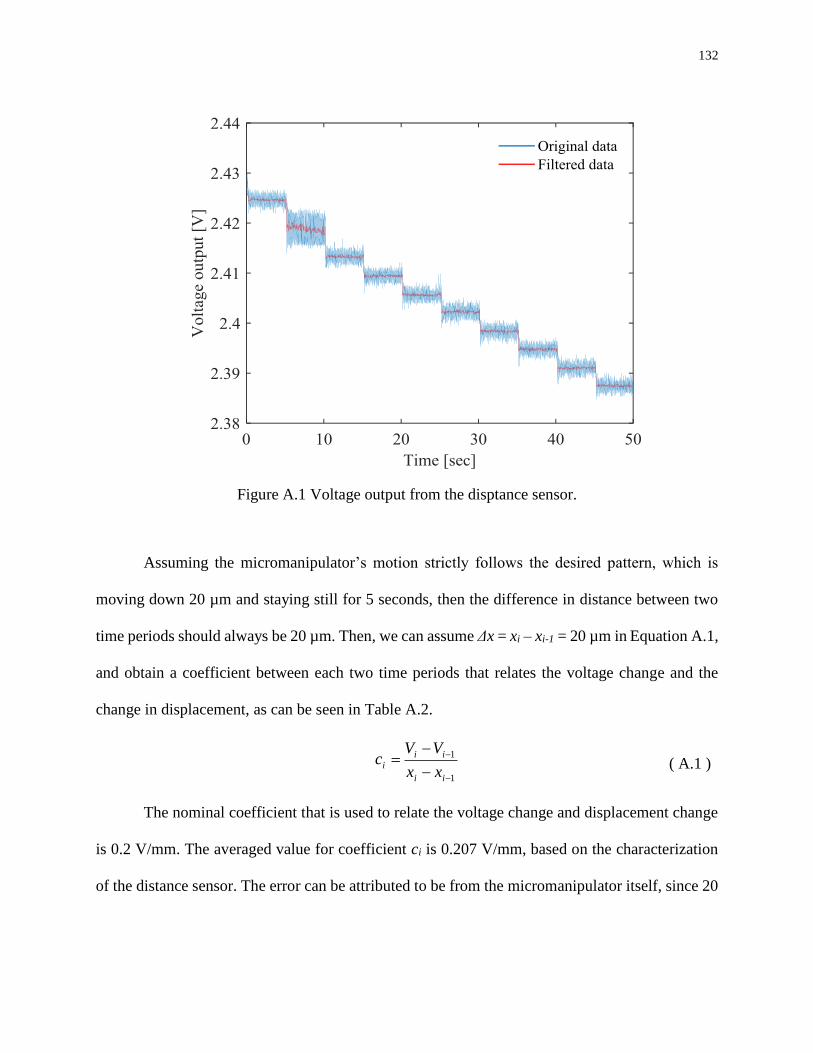
132
Figure A.1 Voltage output from the disptance sensor.
Assuming the micromanipulator’s motion strictly follows the desired pattern, which is
moving down 20 µm and staying still for 5 seconds, then the difference in distance between two
time periods should always be 20 µm. Then, we can assume Δx = xi – xi-1 = 20 µm in Equation A.1,
and obtain a coefficient between each two time periods that relates the voltage change and the
change in displacement, as can be seen in Table A.2.
1
1
ii
iii
xx
VVc ( A.1 )
The nominal coefficient that is used to relate the voltage change and displacement change
is 0.2 V/mm. The averaged value for coefficient ci is 0.207 V/mm, based on the characterization
of the distance sensor. The error can be attributed to be from the micromanipulator itself, since 20
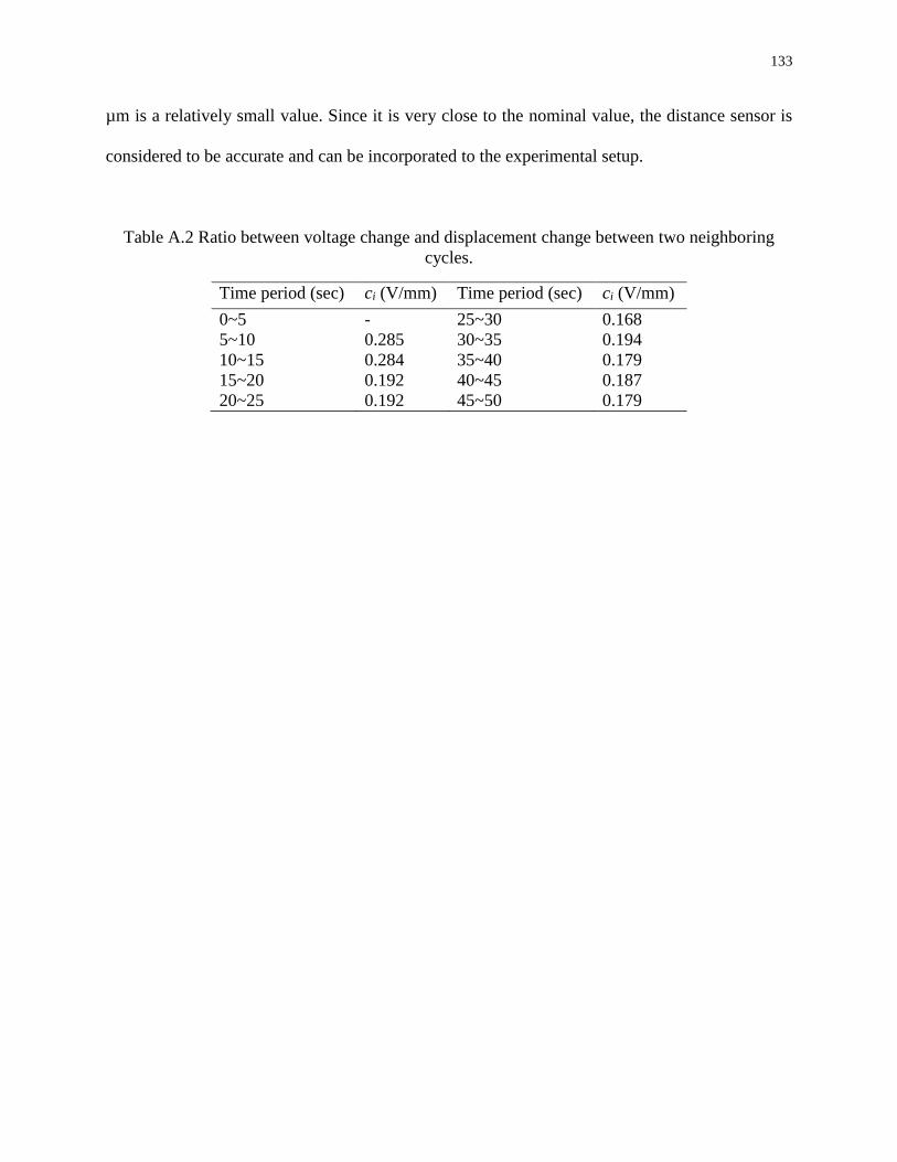
133
µm is a relatively small value. Since it is very close to the nominal value, the distance sensor is
considered to be accurate and can be incorporated to the experimental setup.
Table A.2 Ratio between voltage change and displacement change between two neighboring
cycles.
Time period (sec) ci (V/mm) Time period (sec) ci (V/mm)
0~5 - 25~30 0.168
5~10 0.285 30~35 0.194
10~15 0.284 35~40 0.179
15~20 0.192 40~45 0.187
20~25 0.192 45~50 0.179
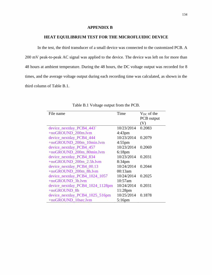
134
APPENDIX B
HEAT EQUILIBRIUM TEST FOR THE MICROFLUIDIC DEVICE
In the test, the third transducer of a small device was connected to the customized PCB. A
200 mV peak-to-peak AC signal was applied to the device. The device was left on for more than
48 hours at ambient temperature. During the 48 hours, the DC voltage output was recorded for 8
times, and the average voltage output during each recording time was calculated, as shown in the
third column of Table B.1.
Table B.1 Voltage output from the PCB.
File name Time VDC of the
PCB output
(V)
device_nextday_PCB4_443`
+noGROUND_200m.lvm
10/23/2014
4:43pm
0.2083
device_nextday_PCB4_444
+noGROUND_200m_10min.lvm
10/23/2014
4:55pm
0.2079
device_nextday_PCB4_457
+noGROUND_200m_80min.lvm
10/23/2014
6:18pm
0.2069
device_nextday_PCB4_834
+noGROUND_200m_2.5h.lvm
10/23/2014
8:34pm
0.2031
device_nextday_PCB4_00.13
+noGROUND_200m_8h.lvm
10/24/2014
00:13am
0.2044
device_nextday_PCB4_1024_1057
+noGROUND_3h.lvm
10/24/2014
10:57am
0.2025
device_nextday_PCB4_1024_1128pm
+noGROUND_8h
10/24/2014
11:28pm
0.2031
device_nextday_PCB4_1025_516pm
+noGROUND_10sec.lvm
10/25/2014
5:16pm
0.1878
135
APPENDIX C
CALIBRATION OF ATI NANO17 LOAD CELL WITH WENGLOR® CP08MHT80
DISTANCE SENSOR
A cone-shaped structure with a weight of 136.4 g is assembled to the load cell. Without
applying any dynamic load, the readouts from the load cell before and after the assembly are
calculated as 0.00236 N and 1.3440 N, respectively. The difference in force equals to the weight
of an object with a mass of 136.8 g. The difference is only 0.4 g, 0.29% of the nominal value,
indicating the measurement of static force by ATI NANO17 load cell is very accurate.
The dynamic calibration of ATI NANO17 with CP08MHT80 is also conducted. The
experimental setup is shown in Figure C.1, the cone-shaped structure is connected to the load cell
which is directly connected to the vibration shaker. Table C.1 shows the experimental results when
the peak to peak value of the power supply of the vibration shaker is equal to 1 V. The first column
of Table C.1 shows the vibration frequency, the second column shows the vibration amplitude of
the cone-shaped structure which represents the vibration amplitude provided by the shaker and is
obtained from the distance sensor. The third column shows the amplitude calculated from the force
sensor, and the forth column presents the theoretical value of the force amplitude, derived from
Equations C 1-5.
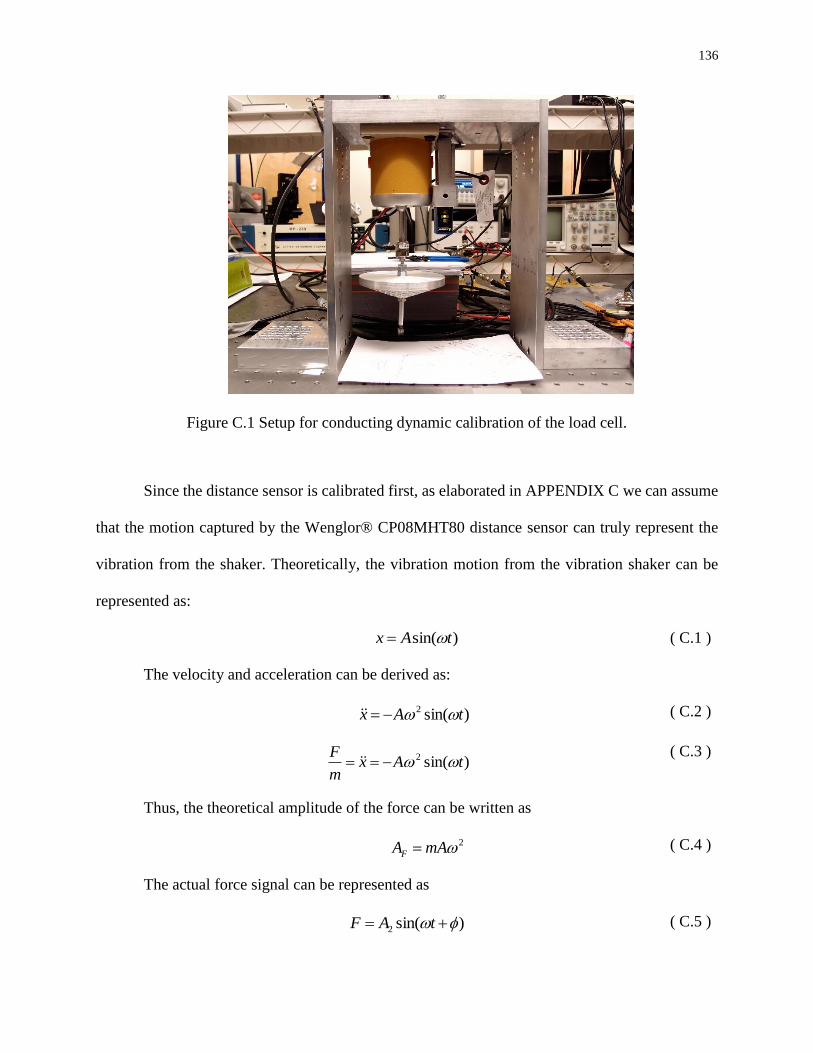
136
Figure C.1 Setup for conducting dynamic calibration of the load cell.
Since the distance sensor is calibrated first, as elaborated in APPENDIX C we can assume
that the motion captured by the Wenglor® CP08MHT80 distance sensor can truly represent the
vibration from the shaker. Theoretically, the vibration motion from the vibration shaker can be
represented as:
)sin( tAx ( C.1 )
The velocity and acceleration can be derived as:
)sin(2 tAx ( C.2 )
)sin(2 tAxm
F
( C.3 )
Thus, the theoretical amplitude of the force can be written as
2mAAF ( C.4 )
The actual force signal can be represented as
)sin(2 tAF ( C.5 )
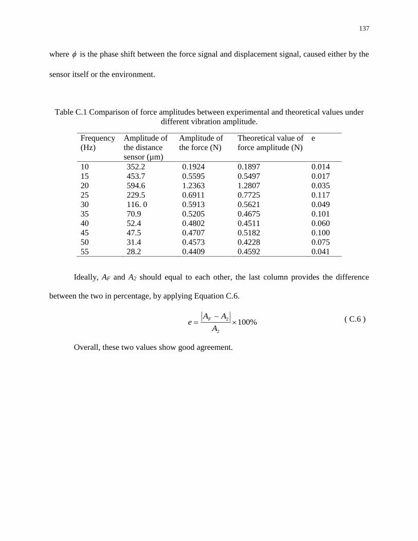
137
where is the phase shift between the force signal and displacement signal, caused either by the
sensor itself or the environment.
Table C.1 Comparison of force amplitudes between experimental and theoretical values under
different vibration amplitude.
Frequency
(Hz)
Amplitude of
the distance
sensor (µm)
Amplitude of
the force (N)
Theoretical value of
force amplitude (N)
e
10 352.2 0.1924 0.1897 0.014
15 453.7 0.5595 0.5497 0.017
20 594.6 1.2363 1.2807 0.035
25 229.5 0.6911 0.7725 0.117
30 116. 0 0.5913 0.5621 0.049
35 70.9 0.5205 0.4675 0.101
40 52.4 0.4802 0.4511 0.060
45 47.5 0.4707 0.5182 0.100
50 31.4 0.4573 0.4228 0.075
55 28.2 0.4409 0.4592 0.041
Ideally, AF and A2 should equal to each other, the last column provides the difference
between the two in percentage, by applying Equation C.6.
%1002
2
A
AAe
F ( C.6 )
Overall, these two values show good agreement.
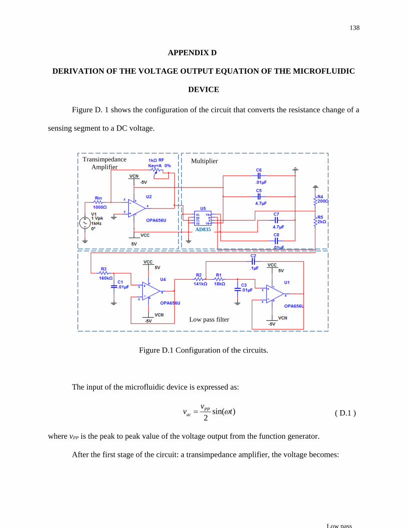
138
APPENDIX D
DERIVATION OF THE VOLTAGE OUTPUT EQUATION OF THE MICROFLUIDIC
DEVICE
Figure D. 1 shows the configuration of the circuit that converts the resistance change of a
sensing segment to a DC voltage.
Figure D.1 Configuration of the circuits.
The input of the microfluidic device is expressed as:
sin( )2
PPac
vv t ( D.1 )
where vPP is the peak to peak value of the voltage output from the function generator.
After the first stage of the circuit: a transimpedance amplifier, the voltage becomes:
Low pass
AD835
Multiplier
Transimpedance
Amplifier
Low pass filter

139
' sin( )2
PP Fac
i
v Rv t
R ( D.2 )
where RF is the resistance of a feedback resistor, and Ri is the resistance of the ith sensing segment
of the microfluidic device, which can be detected by the ith transducer.
Then the amplified voltage goes to the second stage of the circuit: a multiplier and the
voltage after this stage equals to:
2 22
2" sin ( )
4
PP Fac
i
v Rv t
R ( D.3 )
This expression can be further written into:
2 2 2 2
2
2 2" sin ( ) 1 cos(2 )
4 8
PP F PP F
i i
v R v Rv t t
R R ( D.4 )
After the third stage of the circuit, a low pass filter stage, only the DC output remains.
2 2
28
PP Fout
i
v RV
R
( D.5 )
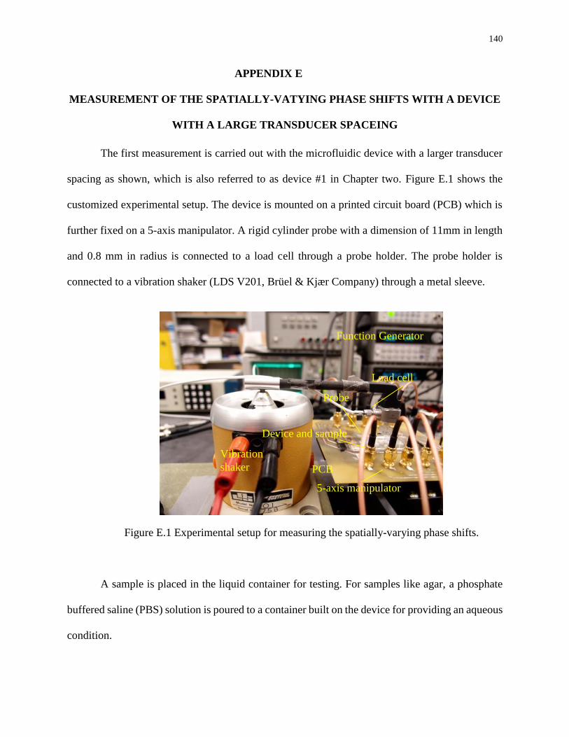
140
APPENDIX E
MEASUREMENT OF THE SPATIALLY-VATYING PHASE SHIFTS WITH A DEVICE
WITH A LARGE TRANSDUCER SPACEING
The first measurement is carried out with the microfluidic device with a larger transducer
spacing as shown, which is also referred to as device #1 in Chapter two. Figure E.1 shows the
customized experimental setup. The device is mounted on a printed circuit board (PCB) which is
further fixed on a 5-axis manipulator. A rigid cylinder probe with a dimension of 11mm in length
and 0.8 mm in radius is connected to a load cell through a probe holder. The probe holder is
connected to a vibration shaker (LDS V201, Brüel & Kjær Company) through a metal sleeve.
Figure E.1 Experimental setup for measuring the spatially-varying phase shifts.
A sample is placed in the liquid container for testing. For samples like agar, a phosphate
buffered saline (PBS) solution is poured to a container built on the device for providing an aqueous
condition.
Function Generator
Vibration
shaker
5-axis manipulator
PCB
Probe
Load cell
Device and sample
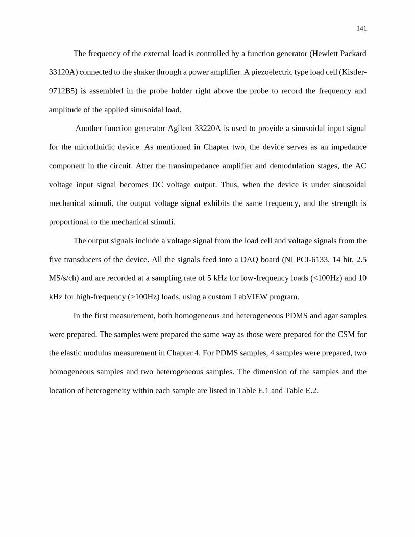
141
The frequency of the external load is controlled by a function generator (Hewlett Packard
33120A) connected to the shaker through a power amplifier. A piezoelectric type load cell (Kistler-
9712B5) is assembled in the probe holder right above the probe to record the frequency and
amplitude of the applied sinusoidal load.
Another function generator Agilent 33220A is used to provide a sinusoidal input signal
for the microfluidic device. As mentioned in Chapter two, the device serves as an impedance
component in the circuit. After the transimpedance amplifier and demodulation stages, the AC
voltage input signal becomes DC voltage output. Thus, when the device is under sinusoidal
mechanical stimuli, the output voltage signal exhibits the same frequency, and the strength is
proportional to the mechanical stimuli.
The output signals include a voltage signal from the load cell and voltage signals from the
five transducers of the device. All the signals feed into a DAQ board (NI PCI-6133, 14 bit, 2.5
MS/s/ch) and are recorded at a sampling rate of 5 kHz for low-frequency loads (<100Hz) and 10
kHz for high-frequency (>100Hz) loads, using a custom LabVIEW program.
In the first measurement, both homogeneous and heterogeneous PDMS and agar samples
were prepared. The samples were prepared the same way as those were prepared for the CSM for
the elastic modulus measurement in Chapter 4. For PDMS samples, 4 samples were prepared, two
homogeneous samples and two heterogeneous samples. The dimension of the samples and the
location of heterogeneity within each sample are listed in Table E.1 and Table E.2.

142
Table E.1 Dimension of the homogeneous samples.
Sample Dimensions(mm)
1:30 PDMS 10.16×6.35×4.46
1:40 PDMS 10×6×4.19
1% agar 10×5.5×4.14
2% agar 10×7×4.07
3% agar 10×6×3.29
Table E.2 Dimension of the heterogeneous samples and the heterogeneity position.
Sample Dimensions(mm) Heterogeneity position
1:30 PDMS 10.16×6.35×3.80 In the middle
1:40 PDMS 10×6×3.81 Three particles, two big ones on the left
1% agar 9×8×5.01 In the middle
2% agar 10.5×7×5.99 In the middle
3% agar 10×6×3.08 In the middle but close to the left
With this setup, the frequency of the input signal varies from 5 Hz to 150 Hz. From the
control experiment, not only the misalignment and microchannel variation are observed, the
resonance of the device is also observed, so that the valid dynamic measurement of material
samples is confined within a certain frequency range. From the data collection side, the sampling
rate for frequencies lower than 100 Hz is set to be 5000, while at frequencies higher than 100 Hz,
the sampling rate is set to be 10,000.
In the measurement, an initial 500 µm deformation is applied to each sample before a
sinusoidal load is added. For homogeneous 1:30 PDMS samples, the frequency was added towards
170 Hz and for homogeneous 1:40 PDMS samples, the frequency was added up to 200 Hz. For
the agar samples, 1% agar samples are tested below 110 Hz for both homogeneous and
heterogeneous samples. 2% agar samples are tested below 140 Hz. For the 3% homogeneous
sample, the frequency range is 1-140 Hz, and the 3% heterogeneous sample is tested every 10 Hz,
up to 200 Hz.
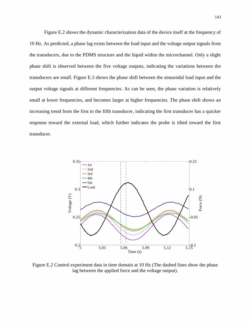
143
Figure E.2 shows the dynamic characterization data of the device itself at the frequency of
10 Hz. As predicted, a phase lag exists between the load input and the voltage output signals from
the transducers, due to the PDMS structure and the liquid within the microchannel. Only a slight
phase shift is observed between the five voltage outputs, indicating the variations between the
transducers are small. Figure E.3 shows the phase shift between the sinusoidal load input and the
output voltage signals at different frequencies. As can be seen, the phase variation is relatively
small at lower frequencies, and becomes larger at higher frequencies. The phase shift shows an
increasing trend from the first to the fifth transducer, indicating the first transducer has a quicker
response toward the external load, which further indicates the probe is tilted toward the first
transducer.
Figure E.2 Control experiment data in time domain at 10 Hz (The dashed lines show the phase
lag between the applied force and the voltage output).
5 5.03 5.06 5.09 5.12 5.150.2
0.25
0.3
0.35
Time (s)
Volt
age
(V)
1st
2nd
3rd
4th
5th
Load
-0.2
-0.05
0.1
0.25
Forc
e (N
)
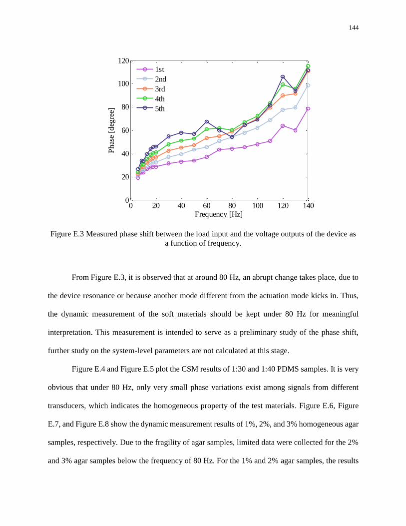
144
Figure E.3 Measured phase shift between the load input and the voltage outputs of the device as
a function of frequency.
From Figure E.3, it is observed that at around 80 Hz, an abrupt change takes place, due to
the device resonance or because another mode different from the actuation mode kicks in. Thus,
the dynamic measurement of the soft materials should be kept under 80 Hz for meaningful
interpretation. This measurement is intended to serve as a preliminary study of the phase shift,
further study on the system-level parameters are not calculated at this stage.
Figure E.4 and Figure E.5 plot the CSM results of 1:30 and 1:40 PDMS samples. It is very
obvious that under 80 Hz, only very small phase variations exist among signals from different
transducers, which indicates the homogeneous property of the test materials. Figure E.6, Figure
E.7, and Figure E.8 show the dynamic measurement results of 1%, 2%, and 3% homogeneous agar
samples, respectively. Due to the fragility of agar samples, limited data were collected for the 2%
and 3% agar samples below the frequency of 80 Hz. For the 1% and 2% agar samples, the results
0 20 40 60 80 100 120 1400
20
40
60
80
100
120
Frequency [Hz]
Ph
ase
[deg
ree]
1st
2nd
3rd
4th
5th

145
are very consistent. When the frequency is below 80 Hz, the variation of the phase shift among
transducers are very small, which proves the homogeneity of the samples under test. For the 3%
agar homogeneous sample, the phase variation among the first four transducers is very small, but
the fifth transducer shows a smaller phase shift than the others. This possibly can be attributed to
uneven thickness in some specific region.
Error bars are all added on the data points for each measurement. The maximum standard
deviation of the measurement for different samples below 80 Hz are shown in Table E.3.
Table E.3 The maximum standard deviation of the measurement for different homogeneous
samples below 80 Hz.
Sample 1:30 PDMS 1:40 PDMS 1% agar 2% agar 3% agar
Maximum standard
deviation (degree)
4.58 7.55 13.18 7.15 2.42
Figure E.4 Relation between phase shift and frequency of a 1:30 homogeneous PDMS
sample.
0 50 100 150 2000
50
100
150
200
250
300
Frequency [Hz]
Ph
ase
[deg
ree]
1st
2nd
3rd
4th
5th
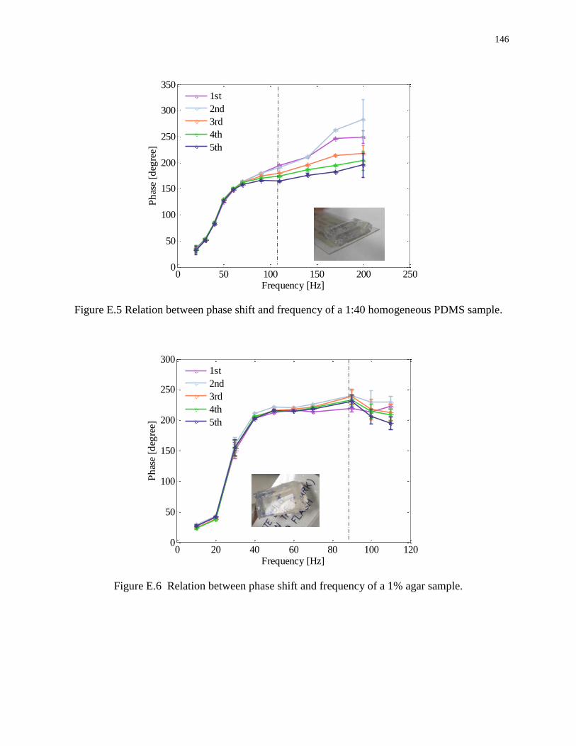
146
Figure E.5 Relation between phase shift and frequency of a 1:40 homogeneous PDMS sample.
Figure E.6 Relation between phase shift and frequency of a 1% agar sample.
0 50 100 150 200 2500
50
100
150
200
250
300
350
Frequency [Hz]
Ph
ase
[deg
ree]
1st
2nd
3rd
4th
5th
0 20 40 60 80 100 1200
50
100
150
200
250
300
Frequency [Hz]
Ph
ase
[deg
ree]
1st
2nd
3rd
4th
5th

147
Figure E.7 Relation between phase shift and frequency of a 2% agar sample.
Figure E.8 Relation between phase shift and frequency of a 3% agar sample.
By comparing the curves in Figure E.9, it can be seen that the phase shifts of transducers
2, 3 and 4 of the 1:30 heterogeneous PDMS sample are much smaller than the rest, indicating the
0 20 40 60 80 100 1200
50
100
150
200
250
300
Frequency [Hz]
Ph
ase
[deg
ree]
1st
2nd
3rd
4th
5th
0 20 40 60 80 100 1200
50
100
150
200
250
Frequency [Hz]
Ph
ase
[deg
ree]
1st
2nd
3rd
4th
5th
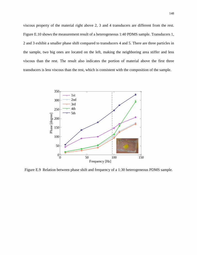
148
viscous property of the material right above 2, 3 and 4 transducers are different from the rest.
Figure E.10 shows the measurement result of a heterogeneous 1:40 PDMS sample. Transducers 1,
2 and 3 exhibit a smaller phase shift compared to transducers 4 and 5. There are three particles in
the sample, two big ones are located on the left, making the neighboring area stiffer and less
viscous than the rest. The result also indicates the portion of material above the first three
transducers is less viscous than the rest, which is consistent with the composition of the sample.
Figure E.9 Relation between phase shift and frequency of a 1:30 heterogeneous PDMS sample.
0 50 100 1500
50
100
150
200
250
300
350
Frequency [Hz]
Ph
ase
[deg
ree]
1st
2nd
3rd
4th
5th
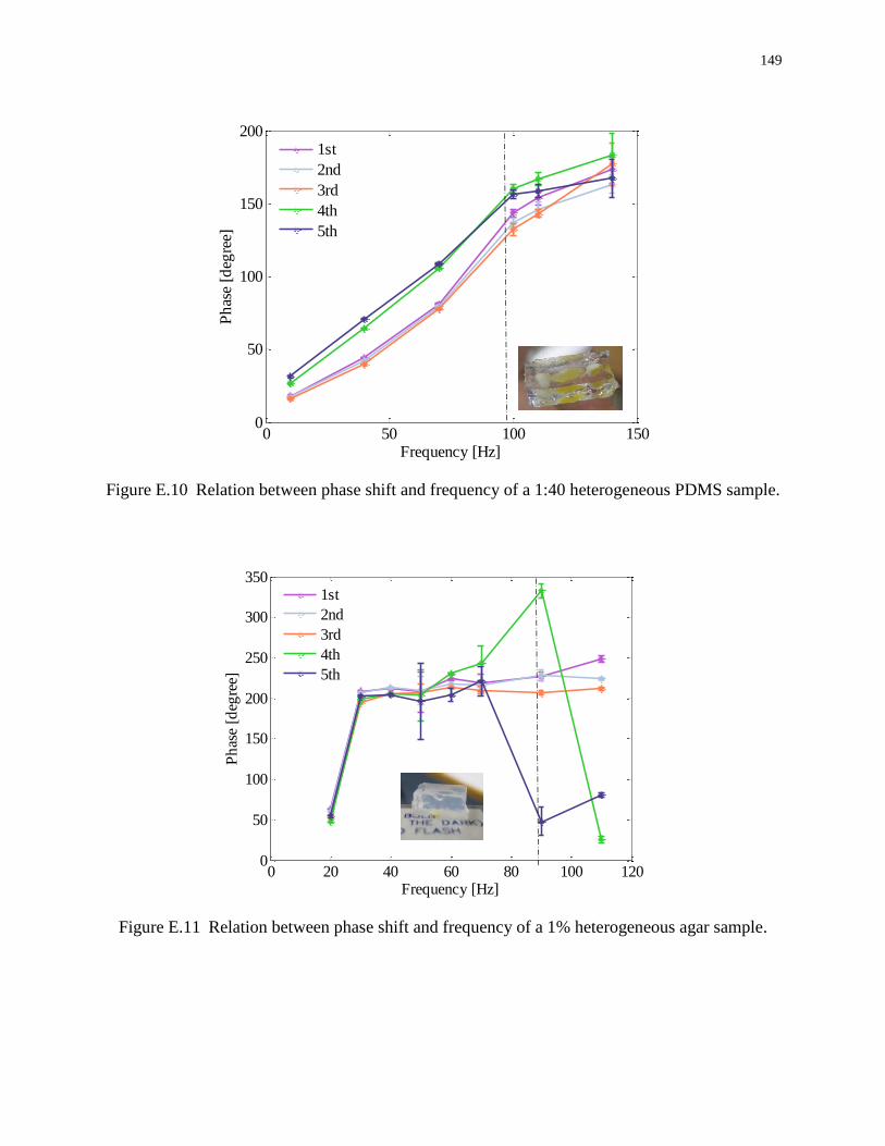
149
Figure E.10 Relation between phase shift and frequency of a 1:40 heterogeneous PDMS sample.
Figure E.11 Relation between phase shift and frequency of a 1% heterogeneous agar sample.
0 50 100 1500
50
100
150
200
Frequency [Hz]
Ph
ase
[deg
ree]
1st
2nd
3rd
4th
5th
0 20 40 60 80 100 1200
50
100
150
200
250
300
350
Frequency [Hz]
Ph
ase
[deg
ree]
1st
2nd
3rd
4th
5th
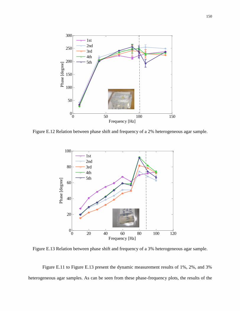
150
Figure E.12 Relation between phase shift and frequency of a 2% heterogeneous agar sample.
Figure E.13 Relation between phase shift and frequency of a 3% heterogeneous agar sample.
Figure E.11 to Figure E.13 present the dynamic measurement results of 1%, 2%, and 3%
heterogeneous agar samples. As can be seen from these phase-frequency plots, the results of the
0 50 100 1500
50
100
150
200
250
300
Frequency [Hz]
Ph
ase
[deg
ree]
1st
2nd
3rd
4th
5th
0 20 40 60 80 100 1200
20
40
60
80
100
Frequency [Hz]
Ph
ase
[deg
ree]
1st
2nd
3rd
4th
5th

151
agar samples are less stable than those of the PDMS samples. The agar samples were tested in a
PBS solution, and are fragile compared with the PDMS samples, making it difficult to obtain stable
results, especially for the 1% and 2% agar samples.
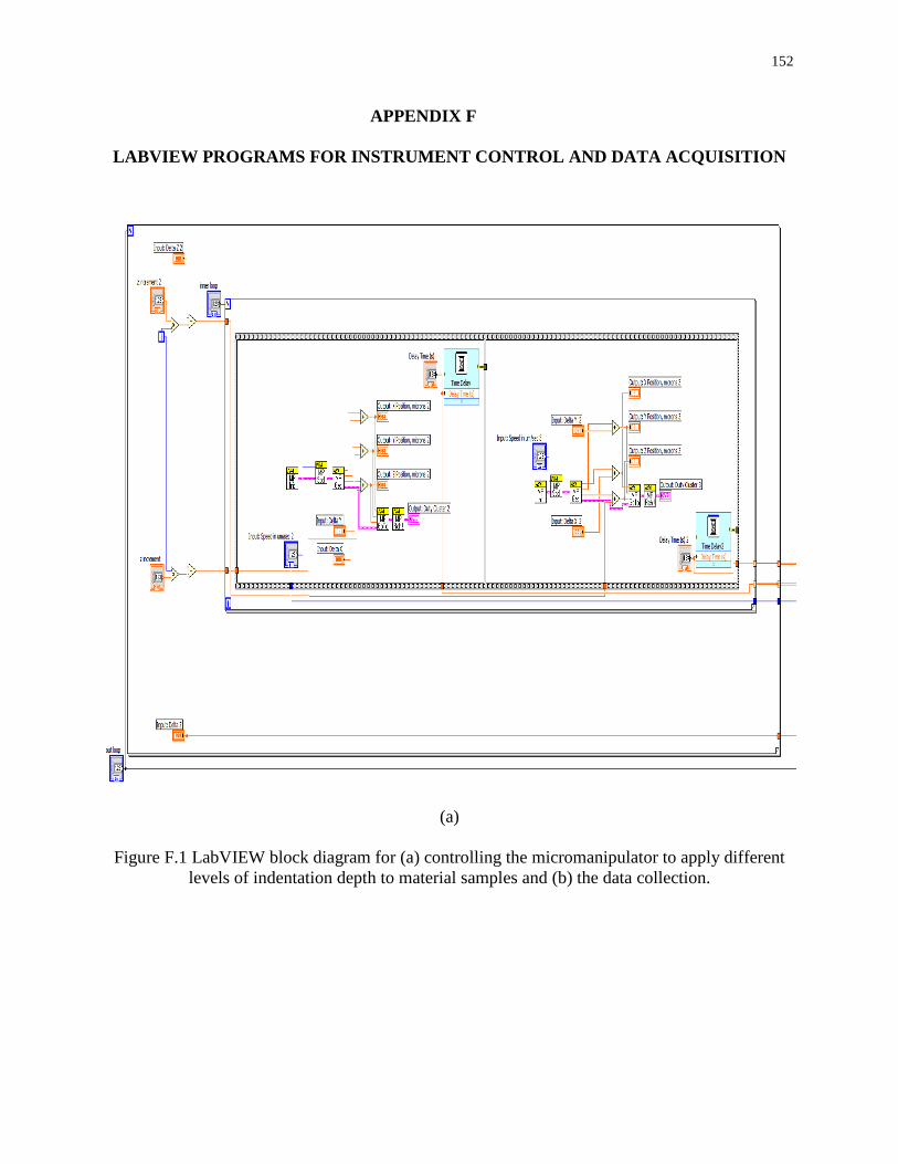
152
APPENDIX F
LABVIEW PROGRAMS FOR INSTRUMENT CONTROL AND DATA ACQUISITION
(a)
Figure F.1 LabVIEW block diagram for (a) controlling the micromanipulator to apply different
levels of indentation depth to material samples and (b) the data collection.
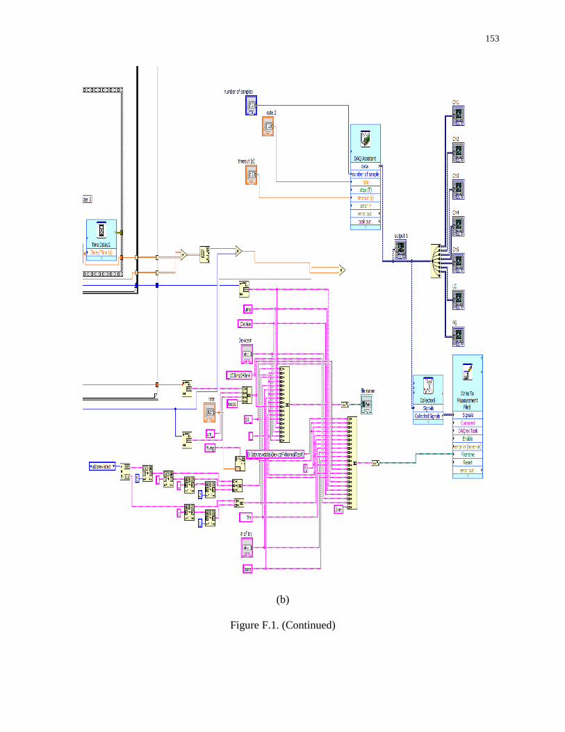
153
(b)
Figure F.1. (Continued)
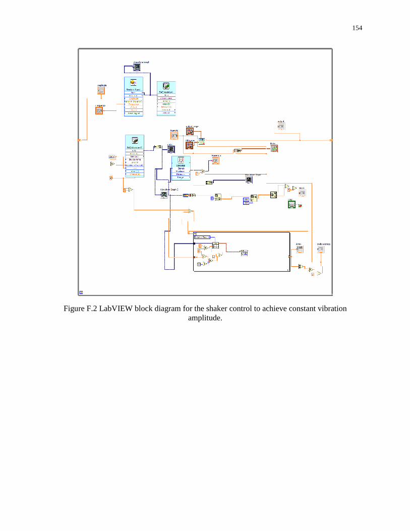
154
Figure F.2 LabVIEW block diagram for the shaker control to achieve constant vibration
amplitude.
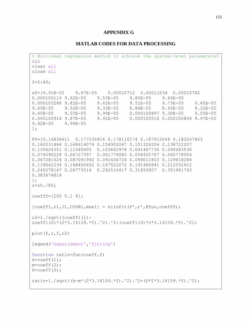
155
APPENDIX G
MATLAB CODES FOR DATA PROCESSING
% Nonlinear regression method to achieve the system-level parameters%
clc
clear all
close all
f=5:40;
z0=[9.91E-05 9.67E-05 0.00010712 0.00011034 0.00010782
0.000100114 9.62E-05 9.53E-05 9.80E-05 9.66E-05
0.000103286 9.82E-05 9.62E-05 9.51E-05 9.73E-05 9.45E-05
9.65E-05 9.52E-05 9.33E-05 8.86E-05 8.93E-05 9.32E-05
9.40E-05 9.55E-05 9.99E-05 0.000100897 9.30E-05 9.55E-05
0.000100916 9.87E-05 9.91E-05 0.000100516 0.000100804 9.97E-05
9.92E-05 9.90E-05
];
F0=[0.16836611 0.177534916 0.178110174 0.187912649 0.183247843
0.162031866 0.168414074 0.154902047 0.151326204 0.138722207
0.135624351 0.11585405 0.103642978 0.091467736 0.090283536
0.076590228 0.06727397 0.061779085 0.056405767 0.060778504
0.067281624 0.087091992 0.091436724 0.099011803 0.129618284
0.139042234 0.148400652 0.167522072 0.191482841 0.212552912
0.245278147 0.26773514 0.292510417 0.31893007 0.351961793
0.383674814
];
r=z0./F0;
coeff0=[200 0.1 9];
[coeff1,r1,J1,COVB1,mse1] = nlinfit(f',r',@fun,coeff0);
r2=1./sqrt((coeff1(1)-
coeff1(2)*(2*3.14159.*f).^2).^2+(coeff1(3)*2*3.14159.*f).^2);
plot(f,r,f,r2)
legend('experiement','fitting')
function ratio=fun(coeff,f)
k=coeff(1);
m=coeff(2);
D=coeff(3);
ratio=1./sqrt((k-m*(2*3.14159.*f).^2).^2+(D*2*3.14159.*f).^2);

156
close all % Codes for obtaining phase shift between force and voltage
output%
clc
clear all
names={
'May 012015_656
PM_try1_sine_10_0.965_5000SR_DeviceEcoflex_200um_100kHz220mV.lvm',...
'May 012015_656
PM_try1_sine_11_0.91_5000SR_DeviceEcoflex_200um_100kHz220mV.lvm',...
'May 012015_657
PM_try1_sine_12_0.88_5000SR_DeviceEcoflex_200um_100kHz220mV.lvm',...
'May 012015_658
PM_try1_sine_13_0.827_5000SR_DeviceEcoflex_200um_100kHz220mV.lvm',...
'May 012015_658
PM_try1_sine_14_0.761_5000SR_DeviceEcoflex_200um_100kHz220mV.lvm',...
'May 012015_659
PM_try1_sine_15_0.729_5000SR_DeviceEcoflex_200um_100kHz220mV.lvm',...
'May 012015_659
PM_try1_sine_16_0.629_5000SR_DeviceEcoflex_200um_100kHz220mV.lvm',...
'May 012015_704
PM_try1_sine_17_0.627_5000SR_DeviceEcoflex_200um_100kHz220mV.lvm',...
'May 012015_709
PM_try1_sine_18_0.484_5000SR_DeviceEcoflex_200um_100kHz220mV.lvm',...
'May 012015_712
PM_try1_sine_19_0.455_5000SR_DeviceEcoflex_200um_100kHz220mV.lvm',...
'May 012015_716
PM_try1_sine_20_0.421_5000SR_DeviceEcoflex_200um_100kHz220mV.lvm',...
'May 012015_723
PM_try1_sine_21_0.344_5000SR_DeviceEcoflex_200um_100kHz220mV.lvm',...
'May 012015_723
PM_try1_sine_22_0.621_5000SR_DeviceEcoflex_200um_100kHz220mV.lvm',...
'May 012015_728
PM_try1_sine_23_0.604_5000SR_DeviceEcoflex_200um_100kHz220mV.lvm',...
'May 012015_730
PM_try1_sine_24_0.644_5000SR_DeviceEcoflex_200um_100kHz220mV.lvm',...
'May 012015_733
PM_try1_sine_25_0.655_5000SR_DeviceEcoflex_200um_100kHz220mV.lvm',...
'May 012015_735
PM_try1_sine_26_0.645_5000SR_DeviceEcoflex_200um_100kHz220mV.lvm',...
'May 012015_737
PM_try1_sine_27_0.862_5000SR_DeviceEcoflex_200um_100kHz220mV.lvm',...
'May 012015_739
PM_try1_sine_28_1.03_5000SR_DeviceEcoflex_200um_100kHz220mV.lvm',...
'May 012015_740
PM_try1_sine_29_1.16_5000SR_DeviceEcoflex_200um_100kHz220mV.lvm',...
'May 012015_742
PM_try1_sine_30_1.18_5000SR_DeviceEcoflex_200um_100kHz220mV.lvm',...
'May 012015_744
PM_try1_sine_31_1.19_5000SR_DeviceEcoflex_200um_100kHz220mV.lvm',...
'May 012015_746
PM_try1_sine_32_1.28_5000SR_DeviceEcoflex_200um_100kHz220mV.lvm',...
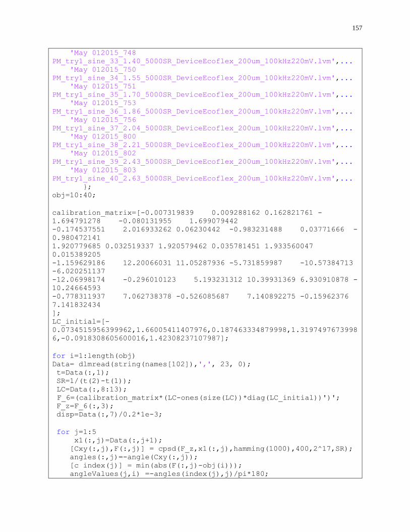
157
'May 012015_748
PM_try1_sine_33_1.40_5000SR_DeviceEcoflex_200um_100kHz220mV.lvm',...
'May 012015_750
PM_try1_sine_34_1.55_5000SR_DeviceEcoflex_200um_100kHz220mV.lvm',...
'May 012015_751
PM_try1_sine_35_1.70_5000SR_DeviceEcoflex_200um_100kHz220mV.lvm',...
'May 012015_753
PM_try1_sine_36_1.86_5000SR_DeviceEcoflex_200um_100kHz220mV.lvm',...
'May 012015_756
PM_try1_sine_37_2.04_5000SR_DeviceEcoflex_200um_100kHz220mV.lvm',...
'May 012015_800
PM_try1_sine_38_2.21_5000SR_DeviceEcoflex_200um_100kHz220mV.lvm',...
'May 012015_802
PM_try1_sine_39_2.43_5000SR_DeviceEcoflex_200um_100kHz220mV.lvm',...
'May 012015_803
PM_try1_sine_40_2.63_5000SR_DeviceEcoflex_200um_100kHz220mV.lvm',...
};
obj=10:40;
calibration_matrix=[-0.007319839 0.009288162 0.162821761 -
1.694791278 -0.080131955 1.699079442
-0.174537551 2.016933262 0.06230442 -0.983231488 0.03771666 -
0.980472141
1.920779685 0.032519337 1.920579462 0.035781451 1.933560047
0.015389205
-1.159629186 12.20066031 11.05287936 -5.731859987 -10.57384713
-6.020251137
-12.06998174 -0.296010123 5.193231312 10.39931369 6.930910878 -
10.24664593
-0.778311937 7.062738378 -0.526085687 7.140892275 -0.15962376
7.141832434
];
LC_initial=[-
0.0734515956399962,1.66005411407976,0.187463334879998,1.3197497673998
6,-0.0918308605600016,1.42308237107987];
for i=1:length(obj)
Data= dlmread(string(names[102]),',', 23, 0);
t=Data(:,1);
SR=1/(t(2)-t(1));
LC=Data(:,8:13);
F_6=(calibration_matrix*(LC-ones(size(LC))*diag(LC_initial))')';
F_z=F_6(:,3);
disp=Data(:,7)/0.2*1e-3;
for j=1:5
x1(:,j)=Data(:,j+1);
[Cxy(:,j),F(:,j)] = cpsd(F_z,x1(:,j),hamming(1000),400,2^17,SR);
angles(:,j)=-angle(Cxy(:,j));
[c index(j)] = min(abs(F(:,j)-obj(i)));
angleValues(j,i) =-angles(index(j),j)/pi*180;
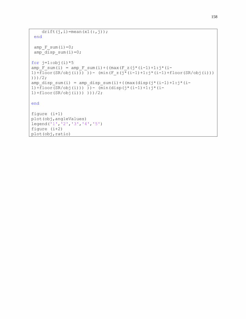
158
drift(j,i)=mean(x1(:,j));
end
amp_F_sum(i)=0;
amp_disp_sum(i)=0;
for j=1:obj(i)*5
amp_F_sum(i) = amp_F_sum(i)+((max(F_z(j*(i-1)+1:j*(i-
1)+floor(SR/obj(i))) ))- (min(F_z(j*(i-1)+1:j*(i-1)+floor(SR/obj(i)))
)))/2;
amp_disp_sum(i) = amp_disp_sum(i)+((max(disp(j*(i-1)+1:j*(i-
1)+floor(SR/obj(i))) ))- (min(disp(j*(i-1)+1:j*(i-
1)+floor(SR/obj(i))) )))/2;
end
figure (i+1)
plot(obj,angleValues)
legend('1','2','3','4','5')
figure (i+2)
plot(obj,ratio)
159
VITA
Wenting Gu received her B.S. degree in Aerospace Engineering from Nanjing University
of Aeronautics and Astronautics in 2009, and received her M.E. degree in Mechanical Engineering
from Old Dominion University in 2013. She is currently a Ph.D. candidate in the Department of
Mechanical and Aerospace Engineering at Old Dominion University. She has been working on the
design, modeling, and characterization of MEMS/Micro sensors since 2010. Her research interests
are developing MEMS/Micro sensors, solving multiphysics problems encountered by
MEMS/Micro sensors, and exploring their applications.