Concrete Semantics of Programs with Non-Deterministic

and Random Inputs

Assale Adje and Jean Goubault-Larrecq

November 3, 2018

Abstract

This document gives semantics to programs written in a C-like programming language,featuring interactions with an external environment with noisy and imprecise data.

1 Introduction

The purpose of this report is to define a concrete semantics for a toy imperative language, meantto incorporate the essential features of languages such as C, as used in numerical control programssuch as those used in the ANR CPP project.

Some of the distinctive aspects of these programs are: the prominent use of floating-pointoperations; and the fact that these programs read inputs from sensors. Both these features implythat the values of numerical program variables are uncertain. Floating-point operations are vul-nerable to round-off errors, which can be modeled as quantization noise. Uncertainty is probablymore manifest with sensors, which return values up to some measurement error. This measure-ment error can be described by giving guaranteed bounds (this is non-determinism: any value inthe interval can be the actual value), or by giving a probability distribution (this is randomness:some values are more likely than others), or a combination of both. To deal with the latter, morecomplex combinations, we rest on variants of two semantic constructions that were studied by thefirst author, previsions [Gou07] and capacities [GL07].

The main goal of a concrete semantics is to serve as a reference. In our case, we wish to be ableto prove the validity of associated abstract semantics and static analysis algorithms, as presentedin other CPP deliverables. The kind of abstract semantics we are thinking of was produced, aspart of CPP, in [BGGP11]. (While it might seem strange that the publication of the abstractsemantics predates the design of the concrete semantics, one might say that both were developedat roughly the same time, with an eye on each other.) So one of our constraints was to ensurethat our concrete semantics should make it easy to justify the abstract semantics we intend.

Before we start, we should also mention an important point. Numerical programs manipulatefloating-point values, which are values from a finite set meant to denote some approximate realvalues. It is customary to think of floating-point values as reals, up to some error. This is whywe shall define a first semantics, called the real semantics, where variables hold actual reals, andno round-off is performed at all. This has well-defined mathematical contents, but is not whatgenuine C programs compute. So we define a second semantics, the floating-point semantics,which is meant to faithfully denote what C programs compute, but works on floating-point data,mathematically an extremely awkward concept: e.g., floating-point addition is not associative, hasone absorbing element (NaN), has no inverse in general (the opposite of infinity inf, −inf, is not aninverse since the sum of inf and −inf is NaN, not 0). But the two semantics are related, throughquantization, which is roughly the process of rounding a real number to the nearest floating-pointvalue.

While the real semantics is much simpler to define than the floating-point semantics withoutrandom choice or non-determinism (e.g., the semantics of + is merely addition), the situation

1

arX

iv:1

210.

2605

v1 [

cs.L

O]

8 O

ct 2

012

changes completely in the presence of random or non-deterministic choice. Let us explain thisbriefly. The prevision semantics of the style presented in [Gou07] is based on continuous mapsand continuous previsions. This is perfectly coherent for ordinary, non-numerical programs (or fornumerical programs in the floating-point semantics, where the type of floating-point numbers ismerely yet another finite data type). However, this is completely at odds with the real semantics.To give a glimpse of the difficulty, one can define the Heaviside function χ[0,+∞) as a numericalC program with real semantics, say by if x < 0 then 0.0 else 1.0, and this is definitely notcontinuous. The deep problem is that, up to some inaccuracies, continuous semantics cannotdescribe more than computable operations, but the real semantics must be non-computable: evenif we restricted ourselves to computable reals, testing whether a computable real is equal to 0 isundecidable.

There are at least two ways to resolve this conundrum. The first one is to cling to the continuoussemantics of random choice and non-determinism of [Gou07] or [GL07], and work not on reals(or tuples of reals, in Rn, representing the list of values of all n program variables), but ratheron a computational model of Rn. The notion of computational model of a topological spaceoriginates from Lawson [Law97]. For example, the dcpo of non-empty closed intervals of reals isa computational model for R, and the Heaviside map would naturally be modeled as the functionmapping every negative real to 0, every positive real to 1, and 0 to the interval [0, 1]. This iselegant, mathematically well-founded, and would allow us to reuse the continuous constructions of[Gou07] or [GL07]. But it falls short of giving an account of real number computation as operatingon reals.

We shall explore the second way here: we shall give a real semantics in terms of measurable,not continuous, maps. This will give us the required degrees of freedom to define our semantics—e.g., the Heaviside map is measurable—while allowing us to define the semantics of random,non-deterministic and mixed choice: anticipating slightly on future sections, this involves gener-alized forms of integration, which will be well-defined precisely on measurable maps. We developthe required theory in sections to come, by analogy with both the classical Lebesgue theory ofintegration and the above cited work on continuous previsions and capacities.

In the presence of random choice only (no non-determinism), our semantics will be isomorphicto Kozen’s semantics of probabilistic programs [Koz81], and his clauses for computing expectationsbackwards will match our prevision-based semantics. The semantics we shall describe in thepresence of other forms of choice (non-deterministic, mixed) are new.

Outline. In Section 2, we introduce the syntax of the programs analyzed. In Section 3, wedefine the maps which are used to pass from floating points to real numbers and vice versa. InSection 4, we define the concrete semantics of expressions and tests and prove the measurabilityof the semantics. In Section 5, we define our concrete semantics based as a continuation-passingsemantics. We also prove in Section 5, the link between our semantics and the theory of previsions.Finally, in Section 6, we treat separately the semantics of the instructions input.

2 Syntax

Let V be a countable set of so-called (program) variables. For each operation op on real numbers,we reserve the symbol op for a syntactic operation meant to implement op (in the real semantics)or some approximation of op (in the floating-point semantics). The syntax of a simple imperativelanguage working on real/floating-point values is given in Figure 1. This syntax does not includeany non-deterministic or probabilistic choice construct: uncertainty will be in the initial values ofthe variables, and will not be created by the program while running.

2

expr ::= a a ∈ Q| x x ∈ V

| −expr| expr+expr| expr−expr| expr×expr| expr/expr

test ::= expr<=expr| expr<expr| expr==expr

| expr ˙! =expr| !test

inst ::= `skip

| `x = expr x ∈ V

| `if test then {inst} else {inst}

| `while test {inst}

| inst ; inst

Figure 1: Syntax of Programs

3 Conversion between Floating Point and Real Numbers

We shall consider two different semantics in Section 4. The first one implements arithmetic withfloating-point numbers, while the second one relies on actual real numbers. Here, we describe thetwo types and how we convert between them.

However, one should first be aware of the pitfalls that are hidden in such a task [Mon08].First and foremost, floating-point numbers are meant to give approximations to real numbers, butfloating-point computations may give values that are arbitrarily far from the corresponding realnumber computation. Monniaux (op. cit., Section 5) gives the example of the following program:

double modulo(double x, double mini, double maxi) {

double delta = maxi-mini;

double decl = x-mini;

double q = decl/delta;

return x - floor(q)*delta

}

int main() {

double m = 180.;

double r = modulo(nextafter(m,0.), -m, m);

}

In a semantics working on real numbers, modulo would return the unique number z in the interval[mini, maxi) such that x−z is a multiple of the interval length maxi−mini. So, certainly, whatevernextafter actually computes, r should be in the interval [−180, 180).

However, running this using IEEE 754 floating-point arithmetic may (and usually will) return−180.0000000000000284 for r. (Here we need to say that nextafter(m,0.) returns the floating-point that is maximal among those that are strictly smaller than m. This has no equivalent in the

3

world of real numbers, and accordingly our language does not include this function.) This is onlylogical:

• When we enter modulo, x is equal to 180− 2−45;

• Then maxi − mini is computed (= 360), and x − mini is computed (= 360 − 2−45); thesevalues are then rounded to the nearest floating-point number, and this is 360 in both cases;

• so delta, decl are both equal to 360, q equals 1;

• so modulo returns (the result of rounding applied to) (180−2−45)−(1×360) = −180−2−45 '−180.0000000000000284.

Of course, the right result, if computed using real numbers instead of floating-point numbers,should be 180− 2−45 ' 179.9999999999999716.

This example can be taken as an illustration of the fact that, even though one can think of eachsingle operation (addition, product, etc.) as being implemented in floating-point computation asthough one first computed the exact, real number result first, and then rounded it, hence obtaininga best possible approximant, this is no longer true for whole programs.

Monniaux goes further, and stresses the fact that various choices in compiler options (e.g.,x87 vs. IEEE 754 arithmetic), IEEE 754 rounding modes, abusive optimization strategies (e.g.,where the compiler uses the fact that addition is associative, which is wrong in floating-pointarithmetic, see op. cit., Section 4.3.2), processor-dependent optimization strategies (e.g., see op.cit., Section 3.2, about the use of the multiply-and-add assembler instruction on PowerPC micro-processors), pragmas (op. cit., Section 4.3.1), all may result in surprising changes in computedvalues.

This causes difficulties in defining sound semantics for floating-point programs, discussed inop. cit., Section 7.3.

But our purpose is not to verify arbitrary numerical programs, and one can make some sim-plifying assumptions:

1. We assume that floating-point arithmetic is performed using the IEEE 754 standard onfloating-point values of a standard, fixed size, typically the 64-bit IEEE 754 (“double”)type. By this, we not only mean that the basic primitives are implemented as the standardprescribes, but that all floating-point values are stored in this format, even when stored inregisters. This is meant to avoid the sundry, dreaded problems mentioned by Monniaux withthe use of x87 arithmetic (where registers hold 80-bit intermediate values).

2. We assume that the rounding mode is fixed, once and for all for all programs. In particular,calls to functions that change the rounding mode on the fly are prohibited.

3. We assume that all optimizations related to floating-point computations are turned off. Thisis meant to avoid abusive (unsound) optimizations (e.g., assuming associativity), and also toavoid processor-dependent optimizations (e.g., compiling a × x + b using a single multiply-and-add instruction: this skips the intermediate rounding that should have occurred whencomputing a× x, and therefore changes the floating-point semantics).

4. We assume that the only floating-point operations allowed are arithmetic operations (i.e.,

+, −, ×, /, but not nextafter for example, or the %f, %g and related directives of printf,scanf and relatives; nor casts to and from the int type—which we shall actually omit).Library functions such as sin, cos, exp, log would be allowable in principle, and theirsemantics would follow the same ideas as presented below—provided we make sure thattheir implementations produce results that are correct in the ulp as well (i.e., that they arecomputed as though the exact result was computed, then rounded; the ulp, a.k.a., the unitin the last place, is the least significant bit of the mantissa).

4

These assumptions allow us to simplify our semantics considerably.Let us go on with the actual data types of floating-point, resp. real numbers. The IEEE

754 standard specifies that, in addition to values representing real numbers, floating-point valuesinclude values denoting +∞ (which we write inf), −∞ (−inf), and silent errors (NaN, for “not anumber”). One can obtain the first two through arithmetic overflow, e.g., by computing 1.0/0.0or −1.0/0.0, and NaNs, e.g., by computing inf− inf. Under Assumption (4) above, there will beno way of distinguishing any such values through the execution of expressions. We abstract themall into a unique symbol err (error).

An added benefit of this abstraction is that it dispenses us from considering the differencebetween the two zeroes, +0.0 and −0.0, of IEEE 754 arithmetic. These are meant to satisfy1.0/inf = +0.0, 1.0/ − inf = −0.0, but are otherwise equal, in the sense that the equalitypredicate applied to +0.0 and −0.0 must return true. Collapsing inf, −inf, and NaN into just onevalue err therefore also allows us to confuse the two zeroes, without harm. This is important ifwe stick to our option that single floating-point operations should computed the exact result thenround: rounding the real number 0 to the nearest would be a nonsense with two floating-pointnumbers representing 0.

The error err is absorbing for all standard arithmetic operations. This means that in oursemantic definitions we assume that the error is propagated during the execution of a programwhich contains these special numbers. Now, we extend by the error symbol err the classical setsof floating points and real numbers, which we denote respectively by F and R. This yields twonew sets: Fe = F ∪ {err} and Re = R ∪ {err}.

Convention 1Let r be in Re. Let � be in {+,−,×, /}. Then:

err � r = r � err = r/0 = −err = err

We consider floating point as special real numbers. Formally, there is a canonical injection injthat lets us to convert a floating-point value (in Fe) into a real number (in Re):

inj : Fe → Ref 7→ inj(f) =

{err if f = errf otherwise

Conversely, there is a projection map projFe: Re → Fe that converts a real number to its

rounded, floating-point representation, as follows. We let Fmin be the smallest floating pointnumber and Fmax be the largest. The projFe

map is required to satisfy the following properties:

• if r /∈ [Fmin,Fmax], then projFe(r) = err;

• if r = inj(f) then projFe(r) = f .

We shall also later require projFeto be measurable (see Proposition 1).

This can be achieved for example by the round-to-nearest function, defined by:

projFe: Re → Fe

r 7→ projFe(r) =

{err if r /∈ [Fmin,Fmax]argmin{|f − r|, f ∈ F} otherwise

When argmin{|f − r|, f ∈ F} contains two elements, the IEEE 754 standard specifies evenrounding, i.e., we take the value f ∈ F whose ulp (last bit of the mantissa) is 0.

4 Concrete Semantics of Expressions and Tests

We now construct two concrete semantics, the first one denoted by J·Kr on real numbers, thesecond one denoted by J·Kf on floating-point values. The construction of these semantics is basedon the two maps inj and projFe

defined above.

5

4.1 Concrete Semantics of Expressions

Every expression will be interpreted in an environment ρ, which serves to specify the values ofvariables. Simply, ρ is a map from the set V of variables to Re (in the real number semantics) orto Fe (in the floating-point semantics). We denote by Σf the set of floating-point environments,and by Σr the set of real number environments.

We start with the semantics in the real model. Let ρr be in Σr. The concrete semantics JexprKrof expressions is constructed in the obvious way:

JaKr(ρr) = aJxKr(ρr) = ρr(x)

J−eKr(ρr) = −JeKr(ρr)Je1+e2Kr(ρr) = Je1Kr(ρr) + Je2Kr(ρr)Je1−e2Kr(ρr) = Je1Kr(ρr)− Je2Kr(ρr)Je1×e2Kr(ρr) = Je1Kr(ρr)× Je2Kr(ρr)Je1/e2Kr(ρr) = Je1Kr(ρr)/Je2Kr(ρr)

The operations are well-defined by Convention 1.Now let us define the floating-point semantics. Let ρf be in Σf . The floating-point semantics

JexprKf of expressions is defined by rounding at the evaluation of each subexpression:

JaKf (ρf ) = projFe(a)

JxKf (ρf ) = ρf (x)J−eKf (ρf ) = projFe

(−inj(JeKf (ρf )))Je1+e2Kf (ρf ) = projFe

(inj(Je1Kf (ρf )) + inj(Je2Kf (ρf )))Je1−e2Kf (ρf ) = projFe

(inj(Je1Kf (ρf ))− inj(Je2Kf (ρf )))Je1×e2Kf (ρf ) = projFe

(inj(Je1Kf (ρf ))× inj(Je2Kf (ρf )))

Je1/e2Kf (ρf ) = projFe(inj(Je1Kf (ρf ))/inj(Je2Kf (ρf )))

4.2 Concrete Semantics of Tests

The semantics of tests is a bit subtler. Although one cannot distinguish inf, −inf, NaN usingexpressions only—this justified, at least partly, our decision to abstract them as a single valueerr—one can distinguish them using tests. Experiments with a C compiler (gcc 4.2.1 here) indeedshow the following behaviors:

a b a==b a!=b a<=b a<b a>=b a>binf inf 1 0 1 0 1 0inf −inf 0 1 0 0 1 1NaN NaN 0 1 0 0 0 0

Note for example that an NaN is not considered equal to itself, that a!=b is the negation of a==bbut a>b is not the negation of a<=b (e.g., when a = b = NaN).

There are two ways we can deal with this phenomenon. Either we abandon the confusionof inf, −inf, NaN as the single value err, which will allow us to replay the above behaviorprecisely, but will incur many complications; or we consider that the semantics of tests must benon-deterministic: not knowing whether err means inf, −inf, NaN, we are forced to considerthat err==err is any value in {0, 1}.

So the semantics of tests will not be a single value, but a set of (Boolean, in {0, 1}) values. Onemay say that our concrete semantics is therefore slightly of an abstract semantics. We count on thefact that err abstracts (so-called silent) errors, and should occur rarely in working programs. (Weare not after detecting subtle errors, but to give reasonable accuracy bounds on actual workingprograms.)

On the other hand, we do not need to specify which semantics, floating-point or real, is meant:both will work in the same way for tests. Let us introduce the new notation J·K?, where ? is either

6

f (floating-point) or r (real). We denote by Σ? the set of environment in this context. Let ρ? bein Σ?.

Je1<=e2K?(ρ?) =

{1} if Je1K?(ρ?) 6= err, Je2K?(ρ?) 6= err, and Je1K?(ρ?) ≤ Je2K?(ρ?){0} if Je1K?(ρ?) 6= err, Je2K?(ρ?) 6= err, and Je1K?(ρ?) > Je2K?(ρ?){0, 1} if Je1K?(ρ?) = err or Je2K?(ρ?) = err

Je1<e2K?(ρ?) =

{1} if Je1K?(ρ?) 6= err, Je2K?(ρ?) 6= err, and Je1K?(ρ?) < Je2K?(ρ?){0} if Je1K?(ρ?) 6= err, Je2K?(ρ?) 6= err, and Je1K?(ρ?) ≥ Je2K?(ρ?){0, 1} if Je1K?(ρ?) = err or Je2K?(ρ?) = err

Je1==e2K?(ρ?) =

{1} if Je1K?(ρ?) 6= err, Je2K?(ρ?) 6= err, and Je1K?(ρ?) = Je2K?(ρ?){0} if Je1K?(ρ?) 6= err, Je2K?(ρ?) 6= err, and Je1K?(ρ?) 6= Je2K?(ρ?){0, 1} if Je1K?(ρ?) = err or Je2K?(ρ?) = err

Je1˙! =e2K?(ρ?) =

{1} if Je1K?(ρ?) 6= err, Je2K?(ρ?) 6= err, and Je1K?(ρ?) 6= Je2K?(ρ?){0} if Je1K?(ρ?) 6= err, Je2K?(ρ?) 6= err, and Je1K?(ρ?) = Je2K?(ρ?){0, 1} if Je1K?(ρ?) = err or Je2K?(ρ?) = err

J!tK?(ρ?) = {1− v | v ∈ JtK?(ρ?)}

The symbols ≤, <, ≥, > in the right-hand sides above are the usual relations on R. So forexample, the semantics of e1<=e2 is well-defined because we only ever compare two elements of ,i.e., two elements of Re other than err.

4.3 Measurability of Concrete Semantics of Expressions and Tests

In the definition of the semantics, we will work with Lebesgue integrals, or notions that generalizethe Lebesgue integral. It is well-known that one cannot posit that every function is integrablewithout causing inconsistencies, and we shall therefore have to check that every function that weintegrate is measurable.

Measurability concerns are (mostly) irrelevant in the floating-point semantics, if we rememberthat F, hence Fe, is finite, and that every function between finite spaces is measurable. But theyare definitely important in the real number semantics.

Measurability is defined relatively to specific σ-algebras. The Borel σ-algebra on R—or, moregenerally, on any topological space—is the smallest σ-algebra that contains all open subsets.

We extend the topology of R to one on Re by extending the standard metric on R to thefollowing:

d(x, y) =

+∞ if x = err or y = err and x 6= y0 if x = y = err

|x− y| if x, y ∈ R

The resulting topology has, as opens, all open subsets of R, the singleton {err}, and their unions.This makes err an (the unique) isolated point of Re. Note that this topology is not the topology ofthe classical one-point (Alexandroff) compactification of R, in which a basis of open neighborhoodsof err would be given by the sets (−∞, a)∪ (b,+∞)∪ {err}, and err would not be isolated. Thelatter would also be a possible choice, but would induce additional, irrelevant complications.

The subspace Fe has the subspace topology: this is just the discrete topology, since Fe is finite.We equip Σr with the smallest topology that makes each map ρ 7→ ρ(x) continuous, for each

x ∈ V. This makes Σr isomorphic to RVe with the product topology.

Similarly, we equip Σf with the subspace topology from Σr. This is also the product topologyon FV

e , up to isomorphism. Note that this is not the discrete topology as soon as V is infinite:indeed, FV

e is compact and infinite in this case, but all compact discrete topological spaces arefinite. This argument is however uselessly subtle: programs only use finitely many variablesanyway, and for V finite, Σf has the discrete topology.

We write B (Σr) and B (Σf ) for the σ-algebras of Borel subsets of Σr and Σf respectively. Bystandard results in topological measure theory (and crucially using the fact that V is countable),these are also the product σ-algebras on the (measure-theoretic) product of V copies of Re, resp.Fe. (This is because Re, Fe are Polish spaces, and the Borel σ-algebra on a countable topological

7

product of Polish spaces coincides with the σ-algebra of the measure-theoretic product of thespaces, each with their Borel σ-algebra.) This is a reassuring statement: it states that we canharmlessly say “product” without having to say whether this is a topological or measure-theoreticproduct. There is no such trap here.

A measurable map f : X → Y is one such that f−1(E) is a Borel subset for every Borel subsetE; it is equivalent to require that, for every open subset U , f−1(U) is Borel. In particular, everycontinuous map is measurable. When Y is second-countable, i.e., has certain so-called basic openssuch that every open subset is the union of countably many basic opens, then f is measurable ifff−1(U) is Borel for every basic open U . We shall use this in proofs; in particular when Y = Re,where we can take the intervals with rational endpoints, and {err}, as basic opens.

One might think that expressions have continuous real semantics, but this is wrong: x/y as afunction of x, y ∈ Re is not continuous at any point of the form (x, 0). But they are measurable.This would be repaired if we had taken the topology of the 1-point compactification of R on Re,but we only need measurability. On the other hand, we really need the topological and measure-theoretic products to coincide, and while this would also be true with the 1-point compactification,the argument would be slightly more complex.

Proposition 1 (Expressions are Measurable)• For every expression e, ρ 7→ JeKr(ρ) is a measurable function from Σr to Re.

• if V is finite or projFeis measurable, then for every expression e, ρ 7→ JeKf (ρ) is a measurable

function from Σf to Fe.

Proof We proceed by induction on expressions. Let a ∈ Q. The function ρ 7→ JaKr(ρ) is a constantfunction and thus it is continuous, hence measurable. Let x ∈ V. The function ρ 7→ JxKr(ρ) is thecoordinate projection on the x coordinate of ρ and thus it is continuous, hence measurable. Thecase of expressions of the form −e, e1+e2, e1−e2, e1×e2 follows by induction hypothesis, usingthe fact that the corresponding operations on Re are continuous. To show this, it suffices to showthat the inverse image of every basic open subset (i.e., open intervals of R, and {err}) is open inΣr. For example, the inverse image of an open subset of R by + is an open subset of R×R, henceof Re × Re, and the inverse image of the basic open subset {err} is (Re × {err}) ∪ ({err} × Re),hence open. The case of e1/e2 is slightly different as / is not continuous on Re × Re. But it ismeasurable, as we now show, by showing that the inverse image of any basic open subset is Borel.The inverse image of any open interval of R is open, since division is continuous at every point(x, y) with y 6= 0. And the inverse image of {err} by / is the union of Re×{err}, of {`}×Re, andof Re × {0}. The first two are open hence Borel, while the last one is the countable intersection⋂n≥1

(Re × (− 1

n,

1

n)), hence is Borel.

The second assertion is trivial if V is finite, in which case all involved σ-algebras are discrete. Inthe general case, it suffices to observe that inj and projFe

are measurable: inj is even continuous,since any function from a discrete space is, and the fact that projFe

is measurable is our assumptionUsing the fact that the composition of measurable functions is measurable, and using a similarinduction as above, we conclude. �

All natural rounding functions projFeare measurable, so the assumptions we are making in

Proposition 1 will be satisfied. E.g.,

Lemma 1The round-to-nearest map, with even rounding, is measurable from Re to Fe.

Proof Since the Borel σ-algebra on Fe is discrete, it is enough to check that the inverse image ofany single element f ∈ Fe is Borel.

If f ∈ (Fmin,Fmax) ∩ F, and if the ulp of f is 0, then this inverse image is [f + f ′

2,f + f ′′

2]

((f + f ′

2,f + f ′′

2) if the ulp of f is not 0), where f ′ is the largest element of F strictly less than f

and f ′′ is the smallest element of F strictly larger than f .

8

If f = Fmin, then the inverse image of f is [Fmin,f + f ′′

2] (if the ulp of f is 0; [Fmin,

f + f ′′

2)

if the ulp of f is not 0), where f ′′ is the smallest element of F strictly larger than f .

If f = Fmax, then the inverse image of f is [f + f ′

2,Fmax] (if the ulp of f is 0; (

f + f ′

2,Fmax]

if the ulp of f is not 0), where f ′ is the largest element of F strictly less than f .

Finally, the inverse image of err is the union of {err}, of (−∞,Fmin), and of (Fmax,+∞).

All these sets are either open, or closed, and in any case Borel. �

Tests are interpreted as maps from Σ? to P∗{0, 1}, where P∗ denotes non-empty powerset, andare thus multifunctions. One of the standard notions of measurability for multifunctions is to saythat, given topological spaces X and Y , f : X → P∗(Y ) is measurable if and only if f−1(♦U) isBorel for every open subset U of Y . (♦U is the set of subsets that intersect U .) If we understandf as a relation between elements of X and elements of Y , this means that the elements x ∈ Xthat are related to some element of a given open subset U should be Borel.

Proposition 2 (Tests are Measurable)For every test t, ρ 7→ JtKr(ρ) is a measurable function from Σr to P∗{0, 1}. If V is finite or projFe

is measurable, then ρ 7→ JtKf (ρ) is a measurable function from Σf to P∗{0, 1}.

Proof It suffices to show that the inverse image of ♦{0} and of ♦{1} are Borel. We proceed byinduction on t. Let ? be either f or r.

If t is of the form e1<=e2, then JtK?(ρ?) contains 0 if and only if Je1−e2K?(ρ?) is in {err} ∪(0,+∞) (if ? = r; in inj−1({err} ∪ (0,+∞)) if ? = f). The latter is open, and Je1−e2K? ismeasurable by Proposition 1, so JtK−1

? (♦{0}) is Borel. Similarly, JtK?(ρ) contains 1 if and only ifJe1−e2K?(ρ) is in {err} ∪ (−∞, 0] (if ? = r; its inverse image by inj if ? = f), which is closed, soJtK−1

? (♦{1}) is Borel. We proceed similarly if t is of the form e1<e2, e1==e2, or e1˙! =e2.

FInally, if t is of the form !t′, JtK−1? (♦{0}) = Jt′K−1

? (♦{1}), and JtK−1? (♦{1}) = Jt′K−1

? (♦{0}),which allows us to conclude immediately. �

5 Weakest Preconditions and Continuation-Passing StyleSemantics

The idea of a continuation-passing style (CPS) semantics is that the value v returned by a givenprogram is not given explicitly. Rather, one passes a continuation parameter κ to the semantics,and the latter is defined so that it eventually calls κ on the final value v.

While this seems like a complicated and roundabout way of defining semantics, this is veryuseful. For example, this allows one to give semantics to exceptions, or to various forms of non-determinism and probabilistic choice [Gou07].

The continuation κ itself is a map from the domain of values to some, usually unspecifieddomain of answers Ans. (In [Gou07], Ans was required to be R+.)

Also, the “final value” of a program should here be understood as the final environment ρ?that represents the state the program is in on termination. So a continuation κ will be a mapfrom Σ? to Ans.

It should also be noted that continuation-passing style semantics are nothing else than a naturalgeneralization of Dijkstra’s weakest preconditions, or the computation of sets of predecessor statesin transition systems. This is obtained by taking Ans = {0, 1}. Then the continuations κ aremerely the indicator maps of subsets E of environments (predicates P on environments), and thecontinuation-passing style denotation of program π in continuation κ is merely the (continuationrepresenting) the set of environments ρ such that evaluating π starting from ρ may terminate withan environment in E (satisfying P ).

Recall that an ω-cpo is a poset in which every ascending sequence x0 ≤ x1 ≤ . . . ≤ xn ≤ . . .has a supremum (a least upper bound).

9

Assumption 1We assume that Ans is an ω-cpo with a smallest element ⊥Ans, and binary suprema.

We write sup for suprema, and reserve↑

sup for suprema of ascending sequences. Assumption 1canbe stated equivalently as: Ans has all countable suprema (including the supremum ⊥Ans of theempty family). If the language had been deterministic (we fall short of this because of the wayerr is dealt with in tests), we would only need Ans to be an ω-cpo, and would not have a need tobinary suprema.

The typical example of such a set Ans of answers is R+ ∪ {+∞}, with its usual ordering.

As usual, we define the semantics of instructions by recursion on syntax:

• skip:

wpJ`1skip, `2K?(κ) = κ

• assignment:

wpJ`1x := e, `2K?(κ) = fun ρ 7→ κ(ρ[x→ JeK?(ρ)])

• sequence:

wpJ`1P ; `2Q, `3K?(κ) = wpJ`1P, `2K?(

wpJ`2Q, `3K?(κ))

• tests:

wpJ`if t then `1P1 else `0P0, `2K?(κ) =

fun ρ 7→ supi∈JtK?(ρ)

(wpJ`iPi, `2K?(κ)

)(ρ)

In other words,

wpJ`if t then `1P1 else `0P0, `2K?(κ) =

fun ρ 7→

(

wpJ`1P1, `2K?(κ))

(ρ) if JtK?(ρ) = {1}(wpJ`0P0, `2K?(κ)

)(ρ) if JtK?(ρ) = {0}

sup((

wpJ`1P1, `2K?(κ))

(ρ),(

wpJ`0P0, `2K?(κ))

(ρ))

if JtK?(ρ) = {0, 1}

The definition of the semantics of a loop, of the form `1while t `2P uses an auxilary map. Wedenote by F(Σ?, Ans) the set ((Σ? → Ans)→ (Σ? → Ans)) i.e. the set of maps from (Σ? → Ans) toitself. We equip (Σ? → Ans) with the pointwise ordering. The set F(Σ?, Ans) is also equipped withthe pointwise ordering: f ≤ g iff for every κ ∈ (Σ? → Ans), for every ρ ∈ Σ?, f(κ)(ρ) ≤ g(κ)(ρ)in Ans. For every countable family (fi)i∈I of elements of F(Σ?, Ans), its supremum sup

i∈Ifi is then

also computed pointwise:

supi∈I

fi : κ 7→(

fun ρ 7→ supi∈I

(fi(κ)(ρ))

).

From this latter definition, we get the following lemma.

Lemma 2The set F(Σ?, Ans) is a ω-cpo with binary suprema, and with a smallest element ⊥F(Σ?,Ans) definedas:

⊥F(Σ?,Ans)(κ) = fun ρ 7→ ⊥Ans, ∀κ : Σ? 7→ Ans .

10

• loops. Given a test t and an instruction `2P, `1, let Ht,`2P,`1

be the map from F(Σ?, Ans) to

F(Σ?, Ans) defined as follows:

(Ht,`2P,`1

(ϕ))

(κ)(ρ) =

(

wpJ`2P, `1K? (ϕ(κ)))

(ρ) if JtK?(ρ) = {1}κ(ρ) if JtK?(ρ) = {0}sup(

(wpJ`2P, `1K? (ϕ(κ))

)(ρ), κ(ρ)) if JtK?(ρ) = {0, 1}

So, for example, wpJ`if t then `1P1 else `0P0, `2K? = Ht,`1P1,`2

(wpJ`0P0, `2K?).

The semantics of the loop `1while t `2P, `3 is the supremum of the sequence ⊥F(Σ?,Ans),Ht,`2P,`3

(⊥F(Σ?,Ans)), Ht,`2P,`3(H

t,`2P,`3(⊥F(Σ?,Ans))), . . . in F(Σ?, Ans), namely:

wpJ`1while t `2P, `3K? = supn∈N

Hn

t,`2P,`3(⊥F(Σ?,Ans))

A more standard definition would have been to let wpJ`1while t `2P, `3K? be defined as the leastfixpoint of H

t,`2P,`3in F(Σ?, Ans). We show below that this would be equivalent. The reason is

that the map Ht,`2P,`3

is ω-Scott-continuous, i.e., is monotone and preserves suprema of ascendingsequences.

We prove this through two lemmas. The first one shows that Ht,`2P,`1

is ω-Scott-continuous

when the maps κ 7→ wpJ`2P, `1K?(κ) are ω-Scott-continuous. This second lemma says that themaps κ 7→ wpJ`2P, `1K?(κ) are actually ω-Scott-continuous.

Lemma 3Let `2P be an instruction. Let t be a test. Assume that the map

κ 7→ wpJ`2P, `1K?(κ) is ω-Scott-continuous , (1)

then:

• The map Ht,`2P,`1

is ω-Scott-continuous.

• The map supn∈N

Hn

t,`2P,`1is ω-Scott-continuous.

• κ 7→ wpJ`1while t `2P, `3K?(κ) is ω-Scott-continuous.

Proof Let us prove the first assertion. Let ϕ,ϕ′ ∈ F(Σ?, Ans) such that ϕ ≤ ϕ′. For everyκ : Σ? 7→ Ans, for every ρ such that JtK?(ρ) = {1},

wpJ`2P, `1K?(ϕ(κ))(ρ) ≤ wpJ`2P, `1K?(ϕ′(κ))(ρ) ,

so:

Ht,`2P,`1

(ϕ)(κ)(ρ) ≤ Ht,`2P,`1

(ϕ′)(κ)(ρ) .

Let (ϕn)n∈N be an ascending sequence in F (Σ?, Ans). We also have:(wpJ`2P, `1K?

(sup↑

n∈Nϕn(κ)

))(ρ) = sup↑

n∈N

(wpJ`2P, `1K? (ϕn(κ))

)(ρ) .

When JtK?(ρ) = {1}, this is equivalent to:

Ht,`2P,`1

(sup↑

n∈Nϕn

)(κ)(ρ) =

(sup↑

n∈NHt,`2P,`1

(ϕn)

)(κ)(ρ) .

11

When JtK?(ρ) = {0}, we obtain the same equality, where now both sides are the constant κ(ρ).When JtK?(ρ) = {0, 1},

Ht,`2P,`1

(sup↑

n∈Nϕn

)(κ)(ρ) = sup

(sup↑

n∈N

(wpJ`2P, `1K? (ϕn(κ))

)(ρ), κ(ρ)

)= sup↑

n∈N

(sup

(wpJ`2P, `1K? (ϕn(κ)) (ρ), κ(ρ)

))=

(sup↑

n∈NHt,`2P,`1

(ϕn)

)(κ)(ρ) .

The second assertion follows from the first, from the fact that compositions of ω-Scott-continuousmaps are again ω-Scott-continuous (hence Hn

t,`2P,`1is ω-Scott-continuous for every n ∈ N), and

that suprema of ω-Scott-continuous are ω-Scott-continuous.The last assertion follows trivially from the second one, using the fact that application (of

maps to ⊥F(Σ?,Ans)) is ω-Scott-continuous. �

Next, we prove that for every instruction `P , for every label `′, the map κ 7→ wpJ`P, `′K?(κ) isω-Scott-continuous.

Lemma 4 (ω-Scott-Continuity of wpJ·K?)For every instruction `P , for every label `′, the map κ 7→ wpJ`P, `′K?(κ) is ω-Scott-continuous.

Proof We proceed by induction on the instructions.• skip. The instruction skip is the identity map from Σ? → Ans to itself, so it is ω-Scott-

continuous.• Assignment. Let κ, κ′ be maps from Σ? to Ans such that κ ≤ κ′. For every ρ ∈ Σ?,

κ(ρ[x → JeK?(ρ)]) ≤ κ′(ρ[x → JeK?(ρ)]). So wpJ`1x := e, `2K? is a monotonic map. Now, weconsider an ascending sequence (κn)n∈N of maps from Σ? to Ans. We have:(

sup↑

n∈N(κn)

)(ρ[x→ JeK?(ρ)]) = sup↑

n∈N(κn(ρ[x→ JeK?(ρ)]))

and then:

wpJ`1x := e, `2K?(

sup↑

n∈Nκn

)= sup↑

n∈NwpJ`1x := e, `2K?(κn) .

• Sequence. By induction hypothesis on `1P and `2Q, the maps κ → wpJ`1P, `2K?(κ) andκ → wpJ`2Q, `3K?(κ) are ω-Scott-continuous. Since the composition of two ω-Scott-continuousmaps is ω-Scott-continuous then the sequence κ→ wpJ`1P ; `2Q, `3K?(κ) is also ω-Scott-continuous.• Tests. By induction hypothesis on `2P and `3Q, the maps κ → wpJ`2P, `4K?(κ) and κ →

wpJ`3Q, `4K?(κ) are ω-Scott-continuous. Since we consider a pointwise order, it suffices to showthat for every ρ ∈ Σ?, κ 7→ wpJ`1 if t then `2P else `3Q, `4K?(κ)(ρ) is ω-Scott-continuous (fromΣ? 7→ Ans to Ans). When we fix ρ ∈ Σ?, we get three cases whether the test is true, false or trueand false. In each case, we conclude that wpJ`1 if t then `2P else `3Q, `4K?(κ) is ω-Scott-continuousby induction hypothesis.• Loops. By induction hypothesis, κ → wpJ`2P, `1K?(κ) is ω-Scott-continuous. Lemma 3

immediately entails that κ 7→ wpJ`1while t `2P, `3K?(κ) is ω-Scott-continuous. �

We introduce a parametric version of classical previsions. Since we work with ω-cpos, we haveto consider [0,+∞], we add arithmetics conventions to deal with +∞.

Convention 2 (Arithmetics in R+ ∪ {+∞})We add the following rules:

• 0× (+∞) = (+∞)× 0 = 0;

• +∞×+∞ = +∞;

12

• For all x ∈ [0,+∞], x+ (+∞) = (+∞) + x = +∞.

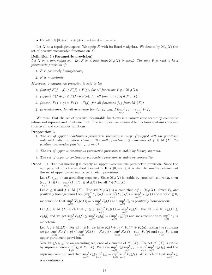
Let X be a topological space. We equip X with its Borel σ-algebra. We denote by M+(X) theset of positive measurable functions on X.

Definition 1 (Parametric prevision)Let X be a non-empty set. Let F be a map from M+(X) to itself. The map F is said to be aparametric prevision if:

1. F is positively homogeneous;

2. F is monotonic;

Moreover, a parametric prevision is said to be:

1. (lower) F (f + g) ≥ F (f) + F (g), for all functions f, g ∈M+(X);

2. (upper) F (f + g) ≤ F (f) + F (g), for all functions f, g ∈M+(X);

3. (linear) F (f + g) = F (f) + F (g), for all functions f, g from M+(X);

4. (ω-continuous) for all ascending family (fn)n∈N, F (sup↑

n∈Nfn) = sup↑

n∈NF (fn).

We recall that the set of positive measurable functions is a convex cone stable by countableinfima and suprema and pointwise limit. The set of positive measurable functions contains constant(positive), and continuous functions.

Proposition 31. The set of upper ω-continuous parametric prevision is ω-cpo (equipped with the pointwise

ordering) with a smallest element (the null pfunctional 0 associates at f ∈ M+(X) thepositive measurable function g : x→ 0)

2. The set of upper ω-continuous parametric prevision is stable by binary suprema.

3. The set of upper ω-continuous parametric prevision is stable by composition.

Proof 1. The parametric 0 is clearly an upper ω-continuous parametric prevision. Since thenull parametric is the smallest element of F(X, [0,+∞]), it is also the smallest element ofthe set of upper ω-continuous parametric previsions.

Let (Fn)n∈N be an ascending sequence. Since M+(X) is stable by countable suprema, then

(sup↑

n∈NFn)(f) = sup↑

n∈N(Fn(f)) ∈M+(X) for all f ∈M+(X).

Let α ≥ 0 and f ∈ M+(X). The set M+(X) is a cone thus αf ∈ M+(X). Since Fn arepositively homogeneous then (sup↑

n∈NFn)(αf) = sup↑

n∈N(Fn(αf)) = sup↑

n∈NαFn(f) and since α ≥ 0,

we conclude that sup↑

n∈N(Fn(αf)) = α sup↑

n∈NFn(f) and sup↑

n∈NFn is positively homogeneous.

Let f, g ∈ M+(X) such that f ≤ g, (sup↑

n∈NFn)(f) = sup↑

n∈NFn(f). For all n ∈ N, Fn(f) ≤

Fn(g) and we get sup↑

n∈NFn(f) ≤ sup↑

n∈NFn(g) = (sup↑

n∈NFn)(g) and we conclude that sup↑

n∈NFn is

monotonic.

Let f, g ∈ M+(X). For all n ∈ N, we have Fn(f + g) ≤ Fn(f) + Fn(g), taking the supremawe get sup↑

n∈NFn(f + g) ≤ sup↑

n∈N(Fn(f) + Fn(g)) ≤ sup↑

n∈NFn(f) + sup↑

n∈NFn(g) and sup↑

n∈NFn is an

upper parametric prevision.

Now let (fk)k∈N be an ascending sequence of elements of M+(X). The set M+(X) is stableby suprema hence sup↑

k∈Nfk ∈M+(X). We have sup↑

n∈NFn(sup↑

k∈Nfk) = sup↑

n∈Nsup↑

k∈NFn(fk) and the

suprema commute and then sup↑

n∈NFn(sup↑

k∈Nfk) = sup↑

k∈Nsup↑

n∈NFn(fk). We conclude that sup↑

n∈NFn

is ω-continuous.

13

2. Let F,G be two upper ω-continuous parametric prevision. From the supremum stabilityproperty, sup(F,G)(f) = sup(F (f), G(f)) belongs to M+(X) for all f ∈M+(X).

Let α ≥ 0 and f ∈ M+(X) (αf ∈ M+(X)), since F,G are positively homogeneous thensup(F,G)(αf) = sup(F (αf), G(αf)) = sup(αF (f), αG(f)) and since α ≥ 0, we concludethat sup(F,G)(αf) = α sup(F (f), G(f)) = α sup(F,G)(f) and sup(F,G) is positively ho-mogeneous.

The supremum of monotonic function is a monotonic function hence sup(F,G) is monotonic.

Let f, g ∈M+(X). We have F (f+g) ≤ F (f)+F (g) and G(f+g) ≤ G(f)+G(g), taking thesupremum we get sup(F,G)(f + g) ≤ sup(F (f) + F (g), G(f) + G(g)) ≤ sup(F (f), G(f)) +sup(F (g), G(g)) = sup(F,G)(f) + sup(F,G)(g) and sup(F,G) is an upper parametric previ-sion.

Now let (fk)k∈nn be an ascending sequence of elements of M+(X) (and thus sup↑

k∈Nfk ∈

M+(X). We have sup(F,G)(sup↑

k∈Nfk) = sup(F (sup↑

k∈Nfk), G(sup↑

k∈Nfk)) = sup(sup↑

k∈NF (fk), sup↑

k∈NG(fk))

and the suprema commute and then sup(F,G)(sup↑

k∈Nfk) = sup↑

k∈Nsup(F,G)(fk). We conclude

that sup(F,G) is ω-continuous.

3. Let F,G be two upper ω-continuous parametric prevision.

Since for all f, g ∈ M+(X), F (f) and G(g) belong to M+(X) then for all h ∈ M+(X),F (G(h)) belongs to M+(X).

Let α ≥ 0 and f ∈ M+(X), since F,G are positively homogeneous then F ◦ G(αf) =F (G(αf)) = F (αG(f)) = αF ◦G(f), we conclude that F ◦G is positively homogeneous.

The composition of two monotonic maps is also monotonic thus F ◦G is monotonic.

Let f, g ∈M+(X). We have G(f+g) ≤ G(f)+G(g), and since F is monotonic, F ◦G(f+g) ≤F (G(f) +G(g)) ≤ F ◦G(f) + F ◦G(g) and F ◦G is an upper parametric prevision.

Now let (fk)k∈nn be an ascending sequence in M+(X). We have F◦G(sup↑

k∈Nfk) = F (G(sup↑

k∈Nfk)) =

F (sup↑

k∈NG(fk)) = sup↑

k∈NF ◦G(fk) and we conclude that F ◦G is ω-continuous.

The main difference between prevision and parametric prevision is the co-domain. Since thedomain and the co-domain are the same, we can compose two parametric previsions to constructa new one. It allows us to think about least fixed points of parametric previsions.

Definition 2 (Previsions)Let X be a non-empty set. Let F be a map from M+(X) to [0,+∞]. The map F is said to be aprevision if:

1. F is positively homogeneous;

2. F is monotonic;

Moreover, a prevision is said to be:

1. (lower) F (f + g) ≥ F (f) + F (g), for all functions f, g ∈M+(X);

2. (upper) F (f + g) ≤ F (f) + F (g), for all functions f, g ∈M+(X);

3. (linear) F (f + g) = F (f) + F (g), for all functions f, g ∈M+(X);

4. (ω-continuous) for all ascending family (fn)n∈N ∈M+(X), F (sup↑

n∈Nfn) = sup↑

n∈NF (fn).

The set M+(X) is equipped with the pointwise ordering. The following proposition shows whythe term parametric appears in Definition 1. The space of parameters is the same of domain ofthe functions of M+(X) i.e. the set X. When we fix a parameter, we get a classical prevision.

14

Proposition 4 (parametric prevision and previsions)The parametric F from M+(X) to itself is a parametric (upper,lower,linear,ω-continuous) previsioniff for all x ∈ X, the map Fx from M+(X) to [0,+∞] defined as Fx(f) = F (f)(x) for all f ∈M+(X) is a (upper,lower,linear,ω-continuous) classical prevision and the maps x → Fx(h) aremeasurable for all h ∈M+(X).

The nondeterminism due to the tests and the value err implies that we cannot expect linearity.Indeed the binary supremum of the sum is not equal to the sum of the suprema, we have only aninequality. In the case of Ans = R+ ∪{+∞}, we can establish that the weakest preconditions andcontinuation-passing style semantics defines an upper parametric prevision. To prove this result,we need a lemma which says that the semantics maps M+(X) to itself.

Lemma 5If κ ∈M+(Σ?), then, for all instructions `1P , wpJ`1P, `2K?(κ) ∈M+(Σ?).

Proof We prove this result by induction on the instructions.• Since the skip is the identity map, thus κ ∈M+(Σ?) implies that wpJ`1skipK?(κ) also belongs

to M+(Σ?).• Now, we consider the assignment. We define the map h : Σ? 7→ Σ? such that at ρ h

associates ρ(y) if y 6= x and JeK?(ρ) otherwise. A coordinate of h is either coordinate projection orthe concrete semantics of an expression which from Proposition 1 is measurable. We conclude thath is measurable since it is componentwise measurable. We conclude that wpJ`1x := e, `2K?(κ) ∈M+(Σ?) (composition of) for all κ ∈M+(Σ?).• Let κ ∈M+(Σ?). The function wpJ`1P ; `2Q, `3K?(κ) is defined as wpJ`1P ; `2K?(wpJ`2Q, `3K?(κ)).

Suppose that wpJ`1P, `2K?(κ′) and wpJ`2Q, `3K?(κ′′) belong to M+(Σ?) for all κ′, κ′′ ∈ M+(Σ?).Then κ′ := wpJ`2Q, `3K?(κ)) is positive and measurable. We conclude that wpJ`1P ; `2K?(κ′) ∈M+(Σ?).• Let κ ∈M+(Σ?). We have:

wpJ`1 if t then `2P else `3Q, `4K?(κ) = sup(

wpJ`1P, `4K?(κ),wpJ`2Q, `4K?(κ))χ{ρ|JtK?(ρ)={0,1}}

+ wpJ`1P, `4K?(κ)χ{ρ|JtK?(ρ)={1}}+ wpJ`2Q, `4K?(κ)χ{ρ|JtK?(ρ)={0}}

Suppose that wpJ`1P, `4K?(κ) and wpJ`2Q, `4K?(κ) are in M+(Σ?). From Proposition 2 thefunctions χ{ρ|JtK?(ρ)=1}, χ{ρ|JtK?(ρ)=0} and χ{ρ|JtK?(ρ)={0,1}} are positive measurable functions. Since

M+(Σ?) is stable by product, sum and binary suprema, thus wpJ`1 if t then `2P else `3Q, `4K?(κ) ∈M+(Σ?).• Let κ ∈M+(Σ?). We have, from Lemma 3:

wpJ`1while t `2P, `3K?(κ) =(

lfp(Ht,`2P,`1

))(κ) =

(sup↑

n∈NHn

t,`2P,`1(⊥F(Σ?,R+))

)(κ)

= sup↑

n∈N

(Hn

t,`2P,`1(⊥F(Σ?,R+))(κ)

)We suppose that wpJ`2P, `1K?(κ′) ∈ M+(Σ?) for all κ′ ∈ M+(Σ?).Since M+(Σ?) is an ω-cpo the

smallest of which is the null function. It suffices to show that for all n ∈ N,(Hn

t,`2P,`1(⊥F(Σ?,R+))

)(κ)

belongs to M+(Σ?). We prove this property by induction on integers. The null function is positive

and measurable. Now, we suppose that there exists an integer n such that(Hn

t,`2P,`1(⊥F(Σ?,R+))

)(κ)

belongs to M+(Σ?). We have:(Hn+1

t,`2P,`1(⊥F(Σ?,R+))

)(κ) = sup

(wpJ`2P, `1K?

((Hn

t,`2P,`1(⊥F(Σ?,R+))

)(κ)), κ)χ{ρ|JtK?(ρ)={0,1}}

+ wpJ`2P, `1K?((Hn

t,`2P,`1(⊥F(Σ?,R+))

)(κ))χ{ρ|JtK?(ρ)={1}}

+κχ{ρ|JtK?(ρ)={0}}

15

From induction hypothesis (on instructions and integers n), Proposition 2 and stability of prod-

uct, sum in M+(Σ?) and binary suprema, we conclude that(Hn+1

t,`2P,`1(⊥F(Σ?,R+))

)(κ) belongs

to M+(Σ?). In conclusion, for all n ∈ N,(Hn

t,`2P,`1(⊥F(Σ?,R+))

)(κ) belongs to M+(Σ?) and

wpJ`1while t `2P, `3K?(κ) ∈M+(Σ?).

Proposition 5When Ans = R+ ∪ {+∞} and X = Σ?, for every instruction `P , for every label `′, wpJ`P, `′K? isan upper ω-continuous parametric prevision.

Proof The fact that for every instruction `P , for every label `′, wpJ`P, `′K? is ω-continuous andmonotonic follows directly from Lemma 4. The measurability has just been proved in Lemma 5.It suffices to show the positive homogeneity and the ”upper condition”. We prove it by inductionon instructions.

• The identity is clearly a linear ω-continuous prevision thus wpJ`skip, `′K? is an upper para-metric prevision.

• Suppose, we have a map g : Σ? → Σ? and consider a map F from M+(Σ?) to itself definedby F (f) = f ◦ g for all f ∈ M+(Σ?). The map F is clearly a linear ω-continuous prevision,this implies that wpJ`1x := e, `2K? is an upper parametric prevision.

• By induction hypothesis, the maps wpJ`2P, `4K? and wpJ`3Q, `4K? are upper parametric pre-visions by Proposition 3 (the third point) wpJ`1P ; `2Q, `3K? is an upper parametric prevision.

• We use Proposition 4. For all ρ such that JtK?(ρ) = {0},

κ 7→ wpJ`1 if t then `2P else `3Q, `4K?(κ)(ρ) =(

wpJ`0P0, `2K?(κ))

(ρ)

which is by induction hypothesis a classical upper prevision. For all ρ such that JtK?(ρ) = {1},the same argument leads to the result. Now suppose that JtK?(ρ) = {0, 1}, by Proposition 3(the second point), we conclude that κ 7→ wpJ`1 if t then `2P else `3Q, `4K?(κ)(ρ) is, by induc-tion hypothesis, a classical upper prevision. The map κ 7→ wpJ`1 if t then `2P else `3Q, `4K?(κ)(ρ)is a classical upper prevision for all ρ ∈ Σ? then wpJ`1 if t then `2P else `3Q, `4K? is an upperparametric prevision.

• By Proposition 3 (the first point), it suffices to prove that the auxilary mapHt,`2P,`3

(⊥F(Σ?,Ans))

is an upper ω-continuous parametric prevision. From Lemma 3, Ht,`2P,`3

(⊥F(Σ?,Ans)) is ω-

continuous and monotonic. It suffices to show that Ht,`2P,`3

(⊥F(Σ?,Ans)) is positively ho-

mogeneous and upper. We prove the result by using Proposition 4. Let ρ ∈ Σ?. Supposethat JtK?(ρ) = {1}. The result follows from the induction hypothesis. Now suppose thatJtK?(ρ) = {0}, H

t,`2P,`3(⊥F(Σ?,Ans)) is the identity and the result follows from the linearity

of the identity. Finally suppose that JtK?(ρ) = {0, 1}, the result follows from the stability ofupper parametric prevision by binary suprema.

6 Special case of inputs

In this subsection, we are interested in interaction between the program and an external environ-ment. This interaction can be viewed as a sensor which saves data from the external environmentthanks to a command input. We suppose that these data are at the same time noisy and imprecise.Mathematically, it can be modelled by ω-capacities. It means that we want to represent for a fixedenvironment ρ the input as a ω-capacity. We assume that only k variables xi1 , xi2 , . . . , xik areaffected by the input.

16

A ω-capacity on a topological space X is a map ν : B (X) 7→ R+ such that:

ν(∅) = 0, ν(U) ≥ 0 and ∀U ∈ B (X) .

The ω-capacity is said to be:

• monotonic iff ∀U, V ∈ B (X):

U ⊆ V =⇒ ν(U) ≤ ν(V ) ;

• continuous iff for all nondecreasing sequences (Un)n∈N ⊆ B (X):

ν

(⋃↑n∈N

Un

)= sup↑

n∈Nν(Un) ;

• convex iff for all U, V ∈ B (X):

ν (U ∪ V ) + ν (U ∩ V ) ≥ ν(U) + ν(V ) ;

• concave iff for all U, V ∈ B (X):

ν (U ∪ V ) + ν (U ∩ V ) ≤ ν(U) + ν(V ) ;

We will use the following result relying convexity and sub(super)linearity of the Choquet integrals.

Proposition 6Let X be a topological space. Let f and g be in M+(X). Let α, β two positive reals.

Let ν be a convex ω-capacity, then the Choquet integral is superlinear:

C

∫x∈X

αf(x) + βg(x)dν ≥ αC∫x∈X

f(x)dν + βC

∫x∈X

g(x)dν

Let µ be a concave ω-capacity, then the Choquet integral is sublinear:

C

∫x∈X

αf(x) + βg(x)dµ ≤ αC∫x∈X

f(x)dµ+ βC

∫x∈X

g(x)dµ

For ρ ∈ Σ?, we suppose that J(xi1 , xi2 , . . . , xik = input()Kc(ρ) is a monotonic continuous ω-capacity ν on VI = {xi1 , xi2 , . . . , xik}. We denote V−I = {x ∈ V, x /∈ VI} and we supposethat a certain ρ0 : V−I 7→ Re (or with value in Fe) is given. We want to extend the ω-capacityJinputKc(ρ) to Re (or Fe) with respect to the fact that the unaffected variables are representedby a fixed environment ρ0. We extend JinputKc(ρ) to a ω-capacity JinputKc(ρ) over Σ? (' RV

e or' FV

e ) as follows:

JinputKc(ρ)(C) = JinputKc(ρ)({x ∈ RVI

e | (x, ρ0) ∈ C})

for all Borel sets C of Σ?. This latter definition means that the measure of a Borel set is completelydetermined by its affected part (by the instruction input).

Assumption 2We assume that ρ 7→ JinputKc(ρ)(U) is measurable for all U ∈ B (Σ?).

We define a last semantics which is the integration of ”continuation” by a ω-capacity. Letκ : Σ? 7→ R+ be a positive measurable function. We define the semantics of the instruction inputas:

wpJinputK?(κ)(ρ) := C

∫ρ′κ(ρ′)dJinputKc(ρ)

17

Proposition 7Under the Assumption 2, for all κ ∈ M+(Σ?), the function ρ 7→ wpJinputK?(κ)(ρ) belongs toM+(Σ?).

Proof The positivity is clear from the definition of the Choquet integral. We only give a prooffor the measurability. Let κ be a positive measurable function. Then κ is the nondecreasingsupremum of a sequence of positive step functions (ϕn)n∈N and:

C

∫x∈X

κ(x)dJinputKc(ρ) = C

∫x∈X

sup↑

n∈Nϕn(x)dJinputKc(ρ) .

From the ω-Scott continuity of Choquet integrals, we get:

C

∫ρ′∈Σ?

κ(ρ′)dJinputKc(ρ) = sup↑

n∈NC

∫ρ′∈Σ?

ϕn(ρ′)dJinputKc(ρ) .

The function ϕn have the form αn

Kn∑i=0

χAni

with (Ani )i is a nonincreasing sequence of Borel sets

for all n ∈ N. Thus, we have:

C

∫ρ′∈X

ϕn(ρ′)dJinputKc(ρ) = αn

Kn∑i=0

JinputKc(ρ)(Ani ) .

Hence, from the Assumption 2, the map ρ 7→ JinputKc(ρ)(Ani ) is measurable for all n ∈ N, for

all i ∈ {0, . . . ,Kn} and then for all n ∈ N, ρ 7→ αn

Kn∑i=0

JinputKc(ρ)(Ani ) is measurable. We conclude

that the map: ρ 7→ C

∫ρ′∈Σ?

κ(ρ′)dJinputKc(ρ) is measurable since it is the pointwise supremum of

measurable functions.

Proposition 8If the ω-capacity JinputKc(ρ) is convex (concave) and ω-continuous then κ 7→ wpJinputK?(κ)(ρ)defines a upper (lower) ω-continuous prevision.

The proof of this latter proposition is left to the reader. Indeed, from Proposition 6, if thecapacity is convex (concave) then the Choquet integral is superlinear (sublinear). The proof isthus reduced to show that if the capacity JinputKc(ρ) is convex or concave then the extendedcapacity JinputKc(ρ) fulfills the same property.

References

[BGGP11] Olivier Bouissou, Eric Goubault, Jean Goubault-Larrecq, and Sylvie Putot. A gen-eralization of P-boxes to affine arithmetic, and applications to static analysis of pro-grams. In Proceedings of the 14th GAMM-IMACS International Symposium on Sci-entific Computing, Computer Arithmetic and Validated Numerics (SCAN’10), Lyon,France, September 2011. To appear.

[GL07] Jean Goubault-Larrecq. Continuous capacities on continuous state spaces. InICALP’2007. Springer-Verlag LNCS, 2007.

[Gou07] Jean Goubault-Larrecq. Continuous previsions. In Jacques Duparc and Thomas A.Henzinger, editors, Proceedings of the 16th Annual EACSL Conference on ComputerScience Logic (CSL’07), pages 542–557, Lausanne, Switzerland, September 2007.Springer-Verlag LNCS 4646.

18

[Koz81] Dexter Kozen. Semantics of probabilistic programs. Journal of Computer and SystemSciences, 22:328–350, 1981.

[Law97] Jimmie Lawson. Spaces of maximal points. Mathematical Structures in ComputerScience, 7:543–555, 1997.

[Mon08] David Monniaux. The pitfalls of verifying floating-point computations. Transactionson Programming Languages and Systems, 30(3), 2008. Article 12.

19