Concrete Plates Designed with FEMProsjektering av betongplater med FEM

Marte Skibeli

Civil and Environmental Engineering

Supervisor: Jan Arve Øverli, KT

Department of Structural Engineering

Submission date: June 2017

Norwegian University of Science and Technology

Department of Structural Engineering Faculty of Engineering NTNU- Norwegian University of Science and Technology

MASTER THESIS 2017

SUBJECT AREA:

Concrete structures

DATE:

6th of June, 2017

NO. OF PAGES:

110+12 pages of appendices TITLE:

Concrete Plates Designed with FEM Prosjektering av betongplater med FEM

BY: Marte Skibeli

RESPONSIBLE TEACHER: Jan Arve Øverli SUPERVISOR(S): Jan Arve Øverli CARRIED OUT AT: Department of Structural Engineering, NTNU

SUMMARY: Most engineering companies design plates by use of finite element programs that are entirely automated. The program decides the element type, the meshing, and performs all the calculations. Often, the automatic procedure is hidden for the user, and it's difficult for the engineer to verify that the analysis is done correctly. Therefore, the goal of this thesis is to describe how concrete plates should be modelled in commercial design software, and how a selection of design programs perform the automatic design procedure. The focus has been on plates subjected primarily to bending in both the Ultimate Limit State (ULS) and in the Serviceability Limit State (SLS). It is normally recommended to model plates with the use of pinned support at the centre of columns or walls, because it avoids unintended rotational restraint. It is, however, also possible to model more realistically, with spring supports, if the stress distribution over the support is of interest, or the rotational restraint from the support is of importance for the stresses in the plate. The main problem of plate design is that, in contrast to simple beam theory, plates also contain twisting moments. This causes the reinforcement and the principal moments to be in different directions. An essential difference between the design procedures in the programs is the assumptions for the stress distribution in the cross section, and the internal lever arm. The programs are also separated by the way they define the crack angle. In SLS, the programs differ in the way the stiffness reduction due to cracks is accounted for. One alternative is to reduce the stiffness locally in elements where the concrete is cracked. Another alternative is to give the whole plate a reduced stiffness to achieve a smooth deformation pattern. The crack width is controlled by either direct calculation of the crack width, or indirect calculation where the diameter and spacing of the reinforcement bars are controlled.

ACCESSIBILITY

OPEN

Preface

This master thesis is written from January to June 2017 for the Department of Structural

Engineering, NTNU, Trondheim.

Numerical calculations based on the finite-element method (FEM) have become a powerful

tool for structural engineers when designing structures. Although the method can do

complex calculations, it is important to remember that the results are no better than the

input from the structural engineer. That is why this thesis will describe how to successfully

model plates with FEM using various loads, boundary conditions, and geometry. The

second part will focus on different methods that commercial software use in the automatic

design of- and capacity control of concrete plates.

I would like to thank my supervisor Jan Arve Øverli for guidance and support, and also

Ola Hansen and Trygve Skibeli for proofreading, and helpful comments.

Marte Skibeli

Trondheim, 6th of June, 2017

i

ii

Summary

Most engineering companies design plates by use of finite element programs that are

entirely automated. The program decides the element type, the meshing, and performs

all the calculations. Often, the automatic procedure is hidden for the user, and it’s

difficult for the engineer to verify that the analysis is done correctly. Therefore, the goal

of this thesis is to describe how concrete plates should be modelled in commercial design

software, and how a selection of design programs perform the automatic design procedure.

The focus has been on plates subjected primarily to bending in both the Ultimate Limit

State (ULS) and in the Serviceability Limit State (SLS).

When modelling a plate, the element type and mesh are often defined automatically by

the software while the boundary conditions need to be specified by the user. It is normally

recommended to use pinned support at the centre of columns or walls, because it avoids

unintended rotational restraint. It is, however, also possible to model more realistically,

with spring supports, if:

• The stress distribution over the support is of interest

• The rotational restraint from the support is of importance for the stresses in the

plate.

The theory background and manuals for a chosen set of design programs were examined

to figure out how the automatic design procedure for concrete plates can be carried out.

The main problem of plate design is that, in contrast to simple beam theory, plates also

contain twisting moments. This causes the reinforcement and the principal moments to

be in different directions. The main steps of the design procedure in ULS are to rotate

the stress resultants to the directions of the reinforcement, and then calculate either the

iii

design moments, or imaginary in-plane forces. These forces are then used to find the

required reinforcement for the upper and lower layer of the plate.

An essential difference between the programs is the assumptions for the stress distribution

in the cross section, and the internal lever arm. The programs are also separated by the

way they define the crack angle. Normally, the crack angle is assumed to be 45o in order

to achieve a minimum amount of reinforcement. If, however, only one reinforcement

direction is needed, the optimal crack angle is no longer 45o. In that case, some of the

programs, like ”FEM design”, calculates a new optimal crack angle.

In SLS, the programs differ in the way the stiffness reduction due to cracks is accounted

for. One alternative is to reduce the stiffness locally in elements where the concrete is

cracked. Another alternative is to give the whole plate a reduced stiffness to achieve a

smooth deformation pattern. The crack width is controlled by either of the following two

approaches:

• Direct calculation of the crack width, and comparing this with the maximum allowed

width

• Indirect calculation where the diameter and spacing of the reinforcement bars are

controlled against tabulated maximum values

iv

Sammendrag

Ved prosjektering av betongdekker blir som regel helautomatiserte elementmetodeprogrammer

benyttet i utregningene. Ofte bestemmer programmene bade elementtype og elementinndeling,

og gjør hele utregningen. Hvordan denne prosessen foregar er ofte skjult for brukeren,

og det blir vanskelig a verifisere at analysen er utført pa rett mate. Malet med denne

oppgaven er derfor a beskrive hvordan betongplater bør modelleres i dataprogrammer

for prosjektering, og hvordan noen utvalgte programmer velger a løse den automatiske

prosjekteringsprosessen. Fokuset i denne oppgaven er plater som hovedsakelig utsettes

for bøyning bade i brudd- og bruksgrensetilstand.

Nar et betongdekke skal modelleres tilbyr som regel programmene automatisk valg av

elementtype og elementinndeling, men opplagere ma brukeren definere selv. For a unnga

utilsiktet fastholdning mot rotasjon anbefales det vanligvis a bruke fritt opplager plassert

midt pa en søyle eller vegg. Det er ogsa mulig a modellere mer realistisk, for eksempel

ved bruk av fjærer, hvis:

• Den faktiske spenningsfordelingen i platen over søylen/veggen er av interesse

• Rotasjonsmotstanden fra opplageret gir store utslag pa spenningene i platen

Hvordan programmene automatiserer prosjekteringsprosessen er studert gjennom a lese

manualene og teorigrunnlaget bak de utvalgte prosjekteringsprogrammene. Hovedproblemet

med a prosjektere plater, sammenlignet med bjelker, er at plater inneholder torsjonsmomenter.

Det gjør at plater ikke far sammenfallende armerings- og hovedmomentsretninger. Hovedtrinnene

i plateprosjektering gar i grove trekk ut pa a rotere spenningsresultantene til de gitte

armeringsretningene, for deretter a finne dimensjonerende moment eller imaginære krefter

i armeringsplanet. Til slutt beregnes nødvendig armeringsmengde i øvre og nedre lag i

v

platen.

En viktig forskjell mellom de ulike programmene er hvordan de antar

trykkspenningsfordelingen i tverrsnittet, og dermed hva den indre momentarmen blir.

I tillegg utgjør definisjonen av rissvinkelen en stor forskjell. Normalt sett gir en valgt

rissvinkel pa 45o minimal armeringsmengde, men dersom det kun er nødvendig med

armering i en retning, sa er ikke lenger 45o rissvinkel optimalt. Noen av programmene,

som for eksempel ”FEM design” beregner da en ny optimal rissvinkel.

I bruksgrensetilstand bruker programmene forskjellige metoder for a ta hensyn til reduksjon

i stivheten pa grunn av rissdannelse. Noen av programmene endrer stivheten lokalt i

elementer der det er for høy spenning, mens andre gir hele platen redusert stivhet slik at

nedbøyningen blir jevn over platen. Rissvidden blir kontrollert ved en av de to følgende

metodene:

• Direkte utregning, og kontroll opp mot maksimal lovlig rissvidde

• Indirekte utregning hvor stangdiameteren og avstanden mellom armeringsstengene

kontrolleres opp mot maksimalt tillate verdier fra tabell

vi

Contents

1 Introduction 1

2 FEM modelling of plates 5

2.1 General . . . . . . . . . . . . . . . . . . . . . . . . . . . . . . . . . . . . . 5

2.2 Material behaviour . . . . . . . . . . . . . . . . . . . . . . . . . . . . . . . 8

2.3 Material parameters . . . . . . . . . . . . . . . . . . . . . . . . . . . . . . 9

2.4 Kirchhoff- and Mindlin-Reissner plates . . . . . . . . . . . . . . . . . . . . 14

2.5 Modelling of support conditions . . . . . . . . . . . . . . . . . . . . . . . . 16

2.5.1 Line supports . . . . . . . . . . . . . . . . . . . . . . . . . . . . . . 17

2.5.2 Column supports . . . . . . . . . . . . . . . . . . . . . . . . . . . . 24

2.6 Modelling of load conditions . . . . . . . . . . . . . . . . . . . . . . . . . . 27

2.7 Singularities . . . . . . . . . . . . . . . . . . . . . . . . . . . . . . . . . . . 28

2.8 Mesh refinement . . . . . . . . . . . . . . . . . . . . . . . . . . . . . . . . . 32

2.9 Choice of control sections . . . . . . . . . . . . . . . . . . . . . . . . . . . . 36

2.9.1 Result sections for moments . . . . . . . . . . . . . . . . . . . . . . 36

2.9.2 Result sections for shear forces . . . . . . . . . . . . . . . . . . . . . 38

2.10 Stress smoothing . . . . . . . . . . . . . . . . . . . . . . . . . . . . . . . . 39

3 Design of plates 45

3.1 General . . . . . . . . . . . . . . . . . . . . . . . . . . . . . . . . . . . . . 45

3.2 Design based on theory of elasticity . . . . . . . . . . . . . . . . . . . . . . 46

3.3 The sandwich model . . . . . . . . . . . . . . . . . . . . . . . . . . . . . . 48

4 Commercial FEM design software 55

4.1 Introduction . . . . . . . . . . . . . . . . . . . . . . . . . . . . . . . . . . . 55

vii

4.2 Design with ”FEM design” . . . . . . . . . . . . . . . . . . . . . . . . . . . 56

4.2.1 Ultimate limit state (ULS) . . . . . . . . . . . . . . . . . . . . . . . 56

4.2.2 Serviceability Limit State (SLS) . . . . . . . . . . . . . . . . . . . . 61

4.2.3 Verification . . . . . . . . . . . . . . . . . . . . . . . . . . . . . . . 62

4.3 Design with ”Robot Structural Analysis Professional” . . . . . . . . . . . . 70

4.3.1 Ultimate Limit State (ULS) . . . . . . . . . . . . . . . . . . . . . . 70

4.3.2 Serviceability Limit State (SLS) . . . . . . . . . . . . . . . . . . . . 74

4.4 Design with ”DIANA” . . . . . . . . . . . . . . . . . . . . . . . . . . . . . 76

4.4.1 Ultimate Limit State (ULS) . . . . . . . . . . . . . . . . . . . . . . 76

4.4.2 Serviceability Limit State (SLS) . . . . . . . . . . . . . . . . . . . . 79

4.4.3 Verification . . . . . . . . . . . . . . . . . . . . . . . . . . . . . . . 80

4.5 Design with ”SOFiSTiK” . . . . . . . . . . . . . . . . . . . . . . . . . . . . 83

4.5.1 Ultimate Limit State (ULS) . . . . . . . . . . . . . . . . . . . . . . 83

4.5.2 Serviceability Limit State (SLS) . . . . . . . . . . . . . . . . . . . . 85

5 Simple beam example 87

5.1 Introduction . . . . . . . . . . . . . . . . . . . . . . . . . . . . . . . . . . . 87

5.2 Strain compatibility . . . . . . . . . . . . . . . . . . . . . . . . . . . . . . . 88

5.3 The sandwich model . . . . . . . . . . . . . . . . . . . . . . . . . . . . . . 89

5.4 ”FEM design” . . . . . . . . . . . . . . . . . . . . . . . . . . . . . . . . . . 89

5.5 ”Robot Structural Analysis” . . . . . . . . . . . . . . . . . . . . . . . . . . 91

5.6 ”DIANA” . . . . . . . . . . . . . . . . . . . . . . . . . . . . . . . . . . . . 91

5.7 Comparison of the different methods . . . . . . . . . . . . . . . . . . . . . 92

6 Discussion and conclusion 93

Bibliography 97

Appendix 101

A Design with ”DIANA” 101

viii

List of Figures

1.1 Example of a bridge with concrete bridge decks [1] . . . . . . . . . . . . . . 1

1.2 Example of precast concrete slabs in a building [2] . . . . . . . . . . . . . . 1

1.3 Stress resultants in a slab [3] . . . . . . . . . . . . . . . . . . . . . . . . . . 4

2.1 Typical elements in commercial software packages [4] . . . . . . . . . . . . 6

2.2 Degrees of freedom for a plate element [3] . . . . . . . . . . . . . . . . . . . 6

2.3 Example of shape functions for a bar element with three nodes [4] . . . . . 7

2.4 Analytical integration (left) and numerical integration with two integration

points (right) [4] . . . . . . . . . . . . . . . . . . . . . . . . . . . . . . . . 7

2.5 Effect of Poisson’s ratio on an element in compression . . . . . . . . . . . . 9

2.6 Moments and curvatures for non-zero Poisson’s ratio [3] . . . . . . . . . . . 10

2.7 Deformation for ν=0 (left) and ν > 0 (right) . . . . . . . . . . . . . . . . . 10

2.8 Bending moment, my, twisting moment, mxy, and corner tie-down force,

Fe, for different Poisson’s ratios ν [5] . . . . . . . . . . . . . . . . . . . . . 11

2.9 Bending moments, my and mx, for different Poisson’s ratios ν . . . . . . . 13

2.10 Comparison of Mindlin and Kirchhoff deformation . . . . . . . . . . . . . . 14

2.11 Comparison of Mindlin and Kirchhoff stresses on a free edge [3] . . . . . . 15

2.12 Linear element (left) and real curvature (right) [4] . . . . . . . . . . . . . . 16

2.13 Different models for hinged line supports [6] . . . . . . . . . . . . . . . . . 17

2.14 Hinge coupling (left), and rigid coupling (right) of nodes over the support [5] 18

2.15 Bending moments for uniform loading at the left span [5] . . . . . . . . . . 19

2.16 Bending moments for uniform loading at both spans (modelled with ”FEM

design”) . . . . . . . . . . . . . . . . . . . . . . . . . . . . . . . . . . . . . 20

2.17 Different ways to model a monolithic connection between a slab and a

supporting wall [6] . . . . . . . . . . . . . . . . . . . . . . . . . . . . . . . 22

ix

2.18 Uplifting of a simply supported slab subjected to uniformly distributed

load [3] . . . . . . . . . . . . . . . . . . . . . . . . . . . . . . . . . . . . . . 22

2.19 Uplifting force in a plate corner . . . . . . . . . . . . . . . . . . . . . . . . 23

2.20 Modelling of discontinuous line supports [5] . . . . . . . . . . . . . . . . . 23

2.21 Point reaction replaced by surface loading [6] . . . . . . . . . . . . . . . . . 25

2.22 Bearing support modelled by spring elements [6] . . . . . . . . . . . . . . . 25

2.23 Bending moment, myy, in section y=0 of a slab supported by corner columns

with different bedding moduli C [5] . . . . . . . . . . . . . . . . . . . . . . 26

2.24 Stresses in a plate for element sizes 0.5 m (left) and 0.02 m (right) when

subjected to a concentrated load (modelled in ”FEM design”) . . . . . . . 28

2.25 Singularity regions [5] . . . . . . . . . . . . . . . . . . . . . . . . . . . . . . 29

2.26 Moment distribution ofmy in sections near the corner of an opening (modelled

with ”DIANA”) . . . . . . . . . . . . . . . . . . . . . . . . . . . . . . . . 30

2.27 Stresses in a re-entrant corner for an element size of 2m (left) and 0.25m

(right) (modelled with ”DIANA”) . . . . . . . . . . . . . . . . . . . . . . . 30

2.28 Bending moment, mxx [kNm/m], in a plate with a re-entrant corner (modelled

with ”FEM design”) . . . . . . . . . . . . . . . . . . . . . . . . . . . . . . 31

2.29 Dispersion of concentrated loads . . . . . . . . . . . . . . . . . . . . . . . . 31

2.30 Member forces of a one-way slab for different numbers of finite elements [5] 33

2.31 Axial deformation and axial stress for a 1D bar with elements of different

polynomial order [4] . . . . . . . . . . . . . . . . . . . . . . . . . . . . . . 34

2.32 Smearing of moment peak [3] . . . . . . . . . . . . . . . . . . . . . . . . . 35

2.33 Moment distribution for different mesh fineness [3] . . . . . . . . . . . . . . 35

2.34 Result section for bending moment in a monolithic connection [6] . . . . . 36

2.35 Result sections for bending moment in a hinged connection with a stiff

support (left) and a soft support (right) [6] . . . . . . . . . . . . . . . . . . 37

2.36 Result section for shear force [6] . . . . . . . . . . . . . . . . . . . . . . . . 38

2.37 Element stress field σ (left), and element smoothed stress field σ∗ (right) [4] 39

2.38 Finite element stress field σ (left), and global smoothed stress field σ∗

(right) [4] . . . . . . . . . . . . . . . . . . . . . . . . . . . . . . . . . . . . 40

2.39 Examples of patches for lower and higher order elements [4] . . . . . . . . 41

2.40 Stresses (top) and stress resultants (bottom) in a bending plate . . . . . . 43

x

3.1 Forces in an infinitesimal plate element [7] . . . . . . . . . . . . . . . . . . 46

3.2 The layers of a sandwich model for a shell element [7] . . . . . . . . . . . . 49

3.3 Compression struts and the angle θ [8] . . . . . . . . . . . . . . . . . . . . 50

3.4 Equilibrium conditions in the compression field theory . . . . . . . . . . . 51

3.5 Different ways to solve a problem of too low concrete compression capacity

[7] . . . . . . . . . . . . . . . . . . . . . . . . . . . . . . . . . . . . . . . . 52

4.1 Coordinate system in ”FEM design” [9] . . . . . . . . . . . . . . . . . . . . 56

4.2 Design moments normal to the reinforcement directions [10] . . . . . . . . 58

4.3 Rectangular stress distribution [8] . . . . . . . . . . . . . . . . . . . . . . . 59

4.4 Example of design output from ”FEM design” [mm2/m] . . . . . . . . . . 60

4.5 Example of peak smoothing with ”FEM design” . . . . . . . . . . . . . . . 61

4.6 The workflow of the stiffness iteration in ”FEM design” . . . . . . . . . . . 62

4.7 Applied edge moments on the plate . . . . . . . . . . . . . . . . . . . . . . 63

4.8 The design moments for hyperbolic bending with orthogonal reinforcement

[kNm/m] . . . . . . . . . . . . . . . . . . . . . . . . . . . . . . . . . . . . . 65

4.9 The required reinforcement for hyperbolic bending with orthogonal reinforcement

in ”FEM design” [mm2/m] . . . . . . . . . . . . . . . . . . . . . . . . . . . 66

4.10 Coordinate-system for calculation with non-orthogonal reinforcement . . . 67

4.11 The required reinforcement for hyperbolic bending with non-orthogonal

reinforcement [mm2/m] . . . . . . . . . . . . . . . . . . . . . . . . . . . . . 69

4.12 The principal moments in the plate [kNm/m] . . . . . . . . . . . . . . . . 69

4.13 Dimensioning of slabs according to Wood & Armer . . . . . . . . . . . . . 71

4.14 Left: Stiffness averaged for all elements. Right: Different stiffness for all

elements [11] . . . . . . . . . . . . . . . . . . . . . . . . . . . . . . . . . . . 75

4.15 Different internal lever arms [7] . . . . . . . . . . . . . . . . . . . . . . . . 77

4.16 Uniaxial stress-strain curve with stress and stiffness reduction [10] . . . . . 80

4.17 Required reinforcement in the y-direction (upper) and in the x-direction

(lower) . . . . . . . . . . . . . . . . . . . . . . . . . . . . . . . . . . . . . . 82

4.18 Stress and strain distributions in the cross-sections [12] . . . . . . . . . . . 84

4.19 Fictitious disks and lever arm for shells [12] . . . . . . . . . . . . . . . . . 84

xi

5.1 Simply supported slab subjected to edge moments, Mx. Side view (top)

and plan view (bottom) . . . . . . . . . . . . . . . . . . . . . . . . . . . . 88

5.2 Required reinforcement from ”FEM design” . . . . . . . . . . . . . . . . . 90

5.3 Required reinforcement in the longitudinal direction, designed with ”DIANA” 91

5.4 Possible strain distribution with rectangular stress distribution . . . . . . . 92

6.1 Different models for stress distribution give different internal lever arms . . 96

xii

Chapter 1

Introduction

Concrete plates are commonly used in structures such as bridges and buildings, from the

smallest cabin to the tallest skyscraper. Figure 1.1 and Figure 1.2 show some examples

of concrete structures.

Figure 1.1: Example of a bridge with concrete bridge decks [1]

Figure 1.2: Example of precast concrete slabs in a building [2]

1

Concrete plates can either be prefabricated, which makes the building process very effective,

or cast-in-place, which makes it possible to create almost all the shapes that a creative

architect may wish for. Consequently, concrete plates are appealing to use, and structural

engineers need to know how to design these plates. The main focus of this thesis will be

on design of concrete plates subjected primarily to bending, such as building floors and

bridge decks. Design for shear will be commented briefly; however, punching shear has

intentionally been left out.

The commercial design software packages available today offer almost endless possibilities

for modelling, and good graphic design makes it intuitive for the structural engineer to

model an arbitrary structure. However, since design software use the Finite Element

Method (FEM), which is an approximate numerical method, it is important to know

what assumptions are made and how they affect the results. Therefore, this master thesis

will describe how to model a concrete plate to achieve proper stress resultants, and how

design software automates the plate design.

The first part of the thesis discusses how to model plates to achieve accurate results for

the internal forces, by correct choice of support conditions, material parameters, mesh

fineness, element type and load application.

The second part of the thesis is about the design procedure for concrete plates. Some of

the design alternatives that are useful for hand calculations are [7]:

• The strip method: A lower-bound design method, where it is assumed that the load

on a plate is dispersed in a certain way in the plate such that the design can be

obtained from a representative set of plate strips. The design forces in the strips can

be calculated with beam theory, and the required reinforcement is found according

to a design code.

• The equivalent frame method: For design of slabs supported by columns. Here, the

plate strips, with center lines above the columns, are regarded as the frame system,

and the maximum and minimum moments are found by calculating a strip in each

2

span direction according to beam theory. The strip width is normally assumed to be

equal to the perpendicular span length. Then, the design moments are distributed

in the perpendicular direction into field strips, outer column strips, and an inner

column strip. Each of these sub-strips are designed separately according to codes.

• The yield line method: Suited for capacity control, in which plastic behaviour

is assumed. The yield lines behave as hinges which carry the constant ultimate

moment of resistance. By use of the virtual work method, the capacity of the

different yield line patterns are found. The yield line pattern with the lowest capacity

gives the dimensioning load capacity. This is an upper-bound approach to find the

load capacity

Even though all the design methods mentioned above can be useful methods, they are

not suited for automatic design in programs. The focus in this thesis will be on design

methods which allow for automatic design performed by software. Chapter 3 will describe

the theory of elasticity and the sandwich model because they are used as basis for the

design in numerous design software. Then, in chapter 4, some commercially available

FEM software will be examined to figure out what design procedure they operate with.

Lastly, chapter 5 consists of a simple calculation example on a beam, in order to compare

the different procedures.

Before discussing details about plate design, it is considered necessary to include information

about the assumptions that are made for plates. Plates in general are planar, spatial

structures that have sides that are at least five times greater than the plate thickness [8].

A plate can either be in the membrane state with only in-plane forces, or in the bending

state with only out-of-plane forces [3]. A concrete plate in the bending state is called a

slab, and normally the following assumptions are made [6]:

• Constant thickness

• The material is homogeneous and isotropic

• Only small vertical displacements (first order theory apply)

3

• No membrane forces

• Linear strain distribution over the section depth. The mid-plane remains strain-less

after loading

• Plane sections normal to the mid-plane remain plane after loading

• Stresses in the normal direction, σzz, are zero

• The strain, εzz, is set to zero. Possible small differences in the displacement over

the thickness of the slab are neglected

The stress resultants for slabs are bending moments in the x- and y-direction, twisting

moments, and vertical shear forces in each direction, as can be seen in Figure 1.3. All of

these internal forces are given per unit length. For thin plates, the shear deformation is

neglected, hence the shear stresses, τxz and τyz, are set to zero. If that is the case, the

shear forces must be derived from the moments rather than by integrating shear stresses.

Figure 1.3: Stress resultants in a slab [3]

4

Chapter 2

FEM modelling of plates

2.1 General

Before going into details about finite-element modelling, a brief introduction will be given

to the basics of the Finite Element Method (FEM). The first step is to subdivide the

structure into a finite number of elements. Some of the standard elements that exists

in commercial software packages today are shown in Figure 2.1. Each element has a set

of nodes associated with them, in which you find generalized forces corresponding to the

Degrees Of Freedom (DOF) in the node. All elements are connected to the neighbouring

elements by enforcing compatibility and equilibrium in the shared nodes. For plates in

bending, it is common to use plane elements with three DOFs per node, one for vertical

displacement and two for rotation around the x- and y-axis respectively, as shown in

Figure 2.2.

5

Figure 2.1: Typical elements in commercial software packages [4]

Figure 2.2: Degrees of freedom for a plate element [3]

6

The deformation field inside an element is determined by use of shape functions that

connect the nodal deformations. To illustrate what shape functions may look like, a bar

element with three nodes and the associated shape functions are showed in Figure 2.3.

The shape function, N1, is a function that is equal to 1 in node 1, and 0 in the other

nodes. N2 is 1 in node 2, and 0 in the other nodes, and so on [4].

Figure 2.3: Example of shape functions for a bar element with three nodes [4]

The deformations are connected to the nodal forces by a stiffness matrix which helps

predict the structural behaviour of the element. The stiffness matrix is found by performing

a numerical integration with integration points inside the element. The integral is solved

by summarizing the values at these integration points and giving each value a specific

weight. For example, if an element has only one integration point, that value would be

fully weighted, while with two integration points each value would get half the weight.

Figure 2.4 illustrates the difference between analytical integration and numerical integration

with two integration points.

Figure 2.4: Analytical integration (left) and numerical integration with two integration

points (right) [4]

7

The most common integration points to use are the Gaussian points. The location of

each Gaussian point, and the weighing of the values can be found in tables; however, this

operation is automatically done by the software. The reason why we use integration points

inside the element instead of the values in the nodes, is that the stresses and strains are

more accurate at the integration points. For more detailed information about the theory

of FEM, see for example Hughes [13].

The recommendations for the modelling of plates (using FEM) is based on the recommendations

presented by Rombach [5], and Pacoste, Plos, and Johansson [6].

2.2 Material behaviour

The response of concrete slabs in bending is highly non-linear due to the cracking and

crushing of concrete and yielding of reinforcement. Nevertheless, it is normal to assume

linear-elastic material behaviour in order to simplify the analysis, and to be able to use

the superposition principle when evaluating the effects of different load cases [6]. The end

result might, however, end up with unrealistic concentrations of moments and forces due

to this simplification. It is therefore important to be aware of this effect in the design to

avoid unnecessary high amounts of reinforcement.

According to the lower-bound theorem of plasticity, linear-elastic analysis can be justified

for the Ultimate Limit State (ULS). The theorem states that if a load on a structure causes

a stress distribution which is within the yield limits, and satisfies both the equilibrium

and statical boundary conditions, then this stress distribution is called safe and statically

admissible, and can’t cause collapse of the body [14]. In linear-elastic analysis, all parts

of the structure will always satisfy both equilibrium and statical boundary conditions;

hence, linear-elastic assumption is always on the safe side when all the stresses present

are below the yield stress.

8

Even though there are some cracks in the concrete which will lead to redistribution of

forces, the assumption of linear-elasticity is considered acceptable in the Serviceability

Limit State (SLS) because the redistribution of stresses is so limited that it can be

neglected [6].

2.3 Material parameters

Based on the assumption that slabs have linear-elastic isotropic material behaviour, only

two material parameters are necessary in the design. That is the modulus of elasticity,

E, and the Poisson’s ratio, ν. The modulus of elasticity, including creep effects, can be

found either from tests, Eurocode 2 (EC2) [8], or other codes for concrete structures. The

Poisson’s ratio is defined as the ratio between the lateral and the axial strain, and varies

between ν = 0.0 and ν = 0.2 for concrete. Figure 2.5 illustrates how deflection in one

direction leads to deflection in the other for ν 6= 0.0. The effect of Poisson’s ratio on the

curvature of an elementary block can be seen from Figure 2.6. The curvature, κ, in one

direction will lead to an additional curvature in the transversal direction equal to ν × κ.

Figure 2.7 shows a deformation model from the program ”FEM design” where a plate is

simply supported at the short edges and subjected to edge moments along the supports.

It can clearly be observed that when ν > 0, the plate gets an additional curvature in the

transverse direction.

Figure 2.5: Effect of Poisson’s ratio on an element in compression

9

Figure 2.6: Moments and curvatures for non-zero Poisson’s ratio [3]

Figure 2.7: Deformation for ν=0 (left) and ν > 0 (right)

10

According to EC2 section 3.1.3(4), the Poisson’s ratio should be set to 0.2 for uncracked

concrete, and 0.0 for cracked concrete. The reason for the reduction in the Poisson’s

ratio when the concrete is cracked is that the tensile forces in the reinforcement can’t be

transmitted through the cracked concrete from one direction to another, so each direction

works independently of each other.

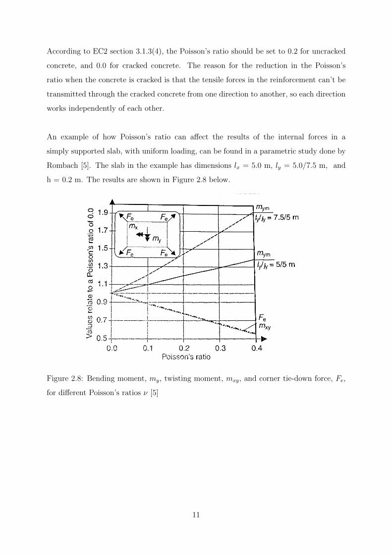
An example of how Poisson’s ratio can affect the results of the internal forces in a

simply supported slab, with uniform loading, can be found in a parametric study done by

Rombach [5]. The slab in the example has dimensions lx = 5.0 m, ly = 5.0/7.5 m, and

h = 0.2 m. The results are shown in Figure 2.8 below.

Figure 2.8: Bending moment, my, twisting moment, mxy, and corner tie-down force, Fe,

for different Poisson’s ratios ν [5]

11

It can be seen from Figure 2.8, on the previous page, that the mid-span bending moment

in the longitudinal direction of the plate, mym, increases almost linearly with increasing

Poisson’s ratio. The greater the ly/lx ratio is, the greater the effect of the Poisson’s ratio

is on the bending moment, mym. This can also be seen from the approximate formulations

of the internal bending moments according to the Kirchhoff theory, shown in Eqs. (2.1)

and (2.2). If one side of the plate is much longer than the other, the shorter direction

is stiffer; hence, it will attract greater moment, and the contribution from this moment,

ν × mν=0x , can be significant for the relatively low bending moment in the longitudinal

direction, mym. Hence, the greater the ly/lx ratio is, the more the Poisson’s ratio will

affect the longitudinal bending moment.

mx ≈ mν=0x + ν ×mν=0

y (2.1)

my ≈ mν=0y + ν ×mν=0

x (2.2)

Figure 2.8 also shows that with increased Poisson’s ratio, the twisting moment, mxy,

and the corner tie-down force, Fe, will decrease linearly. This is also in accordance with

Kirchhoff’s theory formulation for mxy and Fe shown in Eqs. (2.3) and (2.4) respectively,

where K is the flexural rigidity of the slab, and w is the deflection of the slab.

mxy = −K × (1− ν)× (∂2w

∂xy2) (2.3)

Fe = 2×mxy (2.4)

The bending moment in the transverse direction, and the shear forces are not included in

Figure 2.8, because the Poisson’s ratio have only limited effect on them [5].

In order to control the results presented by Rombach [5], the FEM design software ”FEM

design” is used to model a simply supported plate with the dimension 5x7 m being

subjected to a surface load of 10 kN/m2. The results are shown in Figure 2.9, where mxx

is the moment working in the longitudinal direction, and myy in the transverse direction.

12

As expected, the moment in the transverse direction, myy, is greater than the longitudinal

moment, and it doesn’t change much for different Poisson’s ratio. The moment in the

longitudinal direction, mxx, on the other hand changes approximately 45% when the

Poisson’s ratio changes from ν = 0 to ν = 0.2. This result corresponds well with the

graph in Figure 2.8.

Figure 2.9: Bending moments, my and mx, for different Poisson’s ratios ν

13

2.4 Kirchhoff- and Mindlin-Reissner plates

When creating a FEM plate model, it is important to do a deliberate choice between

the Kirchhoff theory and the Mindlin-Reissner theory. Although most commercial FEM

software have one of these theories as default, it does not mean that this assumption is

correct for all structural analysis. This chapter will point out the characteristics for both

theories. Mindlin-Reissner theory is usually referred to as Mindlin theory in FE codes,

and this shorter name will therefore be used hereafter.

Both theories follow the needle hypothesis which implies that if you have a straight needle

perpendicular to the mid-plane of the plate, the needle will remain straight after loading.

Moreover, if the shear force is neglected, the needle will also remain perpendicular to

the mid-plane of the plate. The latter is true only for Kirchhoff theory. Mindlin theory

accounts for shear deformations in the plate, and consequently the shear deformations

might tilt the needle in the x- and/or the y-direction, see Figure 2.10 [3].

Figure 2.10: Comparison of Mindlin and Kirchhoff deformation

14

When the internal forces in a free- or simply supported edge is studied, an important

difference between the two theories becomes clear. Figure 2.11 illustrates how the the

shear force, vx, and the twisting moment, mxy, behaves on a free edge. In a distance

approximately equal to the plate thickness, the twisting moment has to ”turn around” as

illustrated in the top section of Figure 2.11.

Kirchhoff theory handles this by keeping mxy constant up to the edge, and then replacing

all the vertical stresses with a concentrated shear force, V, at the very edge. The

concentrated shear force will have the same numerical value as the twisting moment,

mxy.

Mindlin theory on the other hand, manage to achieve zero twisting moment at the edges

(as it should be), by decomposing the shear stresses into decreasing horizontal stresses

and increasing vertical forces. In order to detect this effect, the edge zone should be

modelled with at least five elements over this short distance [3].

Figure 2.11: Comparison of Mindlin and Kirchhoff stresses on a free edge [3]

15

After this discussion, Mindlin theory might always seem like the correct choice. However,

this is not the case for thin plates, where the edge zone is very small, because then Mindlin

theory requires an unreasonably fine mesh to be able to get accurate results. Moreover,

if Mindlin theory is used on thin plates, shear locking might be a problem. Shear locking

is an error that occurs in linear, quadrilateral elements due to the fact that they fail

to correctly model curvatures of elements, see Figure 2.12. Since the real curvature is

restrained, spurious shear stresses will occur, and the plate will seem stiffer than it is in

reality, and therefore underestimate the displacements. This is only a problem for Mindlin

elements, because Kirchhoff elements ignore the spurious shear strains. The thinner the

plate, the more curvature, and the more erroneous the results will be [4].

Figure 2.12: Linear element (left) and real curvature (right) [4]

Consequently, if the plate is thin enough to neglect shear deformations, one should

use Kirchhoff theory. A span-thickness ratio l/t > 10 is sufficient to neglect the shear

deformations [3].

2.5 Modelling of support conditions

Modelling of the support conditions for slabs should be done with great care as it has

a significant effect on the results. How to model line supports and column supports

correctly, for both hinged- and monolithic connections, is therefore discussed in detail in

this chapter. The recommendations will be simplifications of the real structure, and it is

important that the structural engineer is aware of this, and how it will affect the results.

16

2.5.1 Line supports

The connection between a slab and a continuous wall can be modelled in several ways

depending on:

• The rotational stiffness of the connection

• The thickness of the slab

• The goal of the analysis

Figure 2.13 shows some of the modelling options that are most commonly used for hinged

line supports [6].

Figure 2.13: Different models for hinged line supports [6]

In alternative (a1), the slab is pin-supported in a single node, and this connection is often

called a knife-edge support. The only restraint in this case is the vertical displacement,

at the centre of the support, which corresponds well with beam theory. This is a good

alternative because unintended rotational restraints are avoided. In some cases, however,

the rotational restraint from the wall might be of importance, and in such cases this model

should be avoided. Alternative (a2) is almost similar, with the addition of a rigid link

from the mid-plane of the slab to the support. This option is useful if the plate is thick

17

(a Mindlin plate), and horizontal restraints are present [5].

Alternative (b1) is also pin-supported, but in this case, all the nodes over the support

are coupled to the master node in the middle to simulate an infinite stiff element that

can rotate around the centre. It is important that only the out-of-plane deformation is

restrained, and not the in-plane deformations, because that can cause overconstraining

due to, for instance, temperature loads [6]. The coupling can be either hinged or rigid

as illustrated in Figure 2.14. The rigid connection, shown on the right side of the figure

has basically the same behaviour as alternative (c), and will therefore be discussed later.

With a hinged coupling, the moment distribution corresponds well with beam theory

when only one span is loaded. Figure 2.15 is an illustration presented by Rombach [5],

where a one-way slab with two equal spans of 5 m is subjected to a uniform loading of

10kN/m2 at the left span only. The alternatives with only one pin support, with- and

without hinge coupling, are almost equal, and close to what we would expect from beam

theory.

Figure 2.14: Hinge coupling (left), and rigid coupling (right) of nodes over the support

[5]

18

Figure 2.15: Bending moments for uniform loading at the left span [5]

19

Rombach [5] also argues that the same beam with hinged coupling, subjected to uniform

load at both spans, gives almost similar results as beam theory. However, it is unclear

how the hinged connection is modelled in a program in order to achieve such results since

a very stiff coupling over the support would work as a fully restrained coupling when it is

symmetrically loaded at both sides. To prove this, the same beam as shown in Figure 2.15

is modelled with ”FEM design” for pinned support, hinged coupling, and fully restrained

support in Figure 2.16. It can clearly be seen that the results with hinged coupling are

much closer to the fully restrained model than the pinned support model. Consequently,

the hinged coupling results in too much rotational restraint for uniform loading. For

asymmetric load, however, the hinged coupling allows the beam to rotate more freely

than the fully restrained connection. Similar to the (a2) alternative, the (b2) alternative

applies only to thick plates [5].

Figure 2.16: Bending moments for uniform loading at both spans (modelled with ”FEM

design”)

20

Alternative (c) in Figure 2.13 (page 17) has pinned supports at all nodes over the support

in order to consider the breadth of a very rigid wall. For uniform loading, the moment

at the face of the support will be slightly underestimated, and if the load is asymmetric,

the support moment will be highly overestimated. Alternative (d), with springs in all

the nodes over the support, simulates a flexible, plane support. The results are highly

dependent on the stiffness of the elastic supports which normally is derived from the

stiffness of the wall. This model gives very erroneous results if the stiffness is wrong, and

it is therefore normally recommended to rather simplify by using a simple pin support [5].

In some cases, the normal stiffness of the wall can be of importance for the results. If

so, the entire wall should be included in the model, or alternatively the stiffness of the

wall can be accounted for by translational springs along the centre line of the wall. This

arrangement can be useful if the slab is supported on a wall with interruptions such as

doors and windows [6].

If the slab and the wall are monolithically connected, the wall should preferably be

included in the model because assuming either fixed or pinned support will be too coarse.

If only the stresses in the slab is of interest, it is sufficient to model the bottom of the

wall as either pinned or fixed. In Figure 2.17, two alternative models for monolithic

connections are shown. Alternative (a) has a stiff coupling at the column top with a

height corresponding to half the slab thickness, t. This can give accurate results if the

slab thickness is at least half the size of the wall thickness, ”a”, and ”a” is smaller than the

distance from the wall centre to the nearest point of zero moment for permanent loads, l0.

If ”a” << l0, the stiff coupling can be left out. Alternative (b) has a stiff coupling over the

entire connection zone, including a rigid link on top of the column similar to alternative

(a), and in addition a rigid link in the slab which connects all the nodes over the wall

width. This connection is stiffer than alternative (a); therefore, the support moment will

be greater, and the field moment will consequently decrease [6]. Another alternative is

to simply increase the thickness of the slab locally over the support, and in that way

considering the increased stiffness.

21

Figure 2.17: Different ways to model a monolithic connection between a slab and a

supporting wall [6]

If a thin slab has supports with limited tensile restraint, there might be a problem with

uplifting in the corners, due to twisting moments, as shown in Figure 2.18. This can

happen in building floors if the weight from the wall above is insufficient. The uplifting

force is the sum of the two concentrated Kirchhoff’s shear forces from the meeting edges,

as shown in Figure 2.19. The analysis of such a problem is highly non-linear, yet it can be

solved with a linear-elastic program in an iterative way. First, all the nodes at the edge

are restrained in the vertical direction, then one node after the other from the corners are

released until the analysis show only compressive stresses at the edge. Such an analysis

can be done with vertical springs or special boundary elements with no tensile stiffness.

The uplifting effect results in reduced twisting moments at the corners at the cost of

greater bending moment, greater mid-span deflection, and greater support reactions per

unit length due to reduced supported length. It is wise to be aware of this phenomenon

if tensile support reactions are limited [3].

Figure 2.18: Uplifting of a simply supported slab subjected to uniformly distributed load

[3]

22

Figure 2.19: Uplifting force in a plate corner

If a line support is discontinuous, there will be numerical problems in the analysis due

to the sudden change in boundary conditions. At the unsupported edges, both the shear

force and the bending moment will apparently tend to infinity. However, in reality, the

non-linear material behaviour of concrete will prevent this. Since such non-linear analysis

are very complicated, there are some other alternatives for modelling discontinuous line

supports, shown in Figure 2.20 [5].

Figure 2.20: Modelling of discontinuous line supports [5]

One alternative is to ignore the missing supports and separately design a strip with

sufficient reinforcement to behave as a rigid beam over the discontinuity. This solution is

applicable if the length of the opening is less than 15 times the slab thickness. Another

solution is to reduce the peak values at the unsupported edges by introducing elastic

supports close to the opening. Both of these previous alternatives overcome the numerical

problem of discontinuous line support, but only when looking at the overall behaviour of

the slab. The complex stress and strain distribution at the unsupported edge can’t be

modelled with plain plate elements. A third alternative is to model the opening with shell

or volume elements, but this is complicated and time consuming [5].

23

2.5.2 Column supports

Slabs supported on columns are called flat slabs, and are very commonly used. When flat

slabs are subjected to uniformly distributed load, the load bearing behaviour is nearly

axisymmetric around the supports [6]. The column supports can be modelled very similar

to the line supports, shown previously in Figure 2.13 (page 17) for hinged connections, and

Figure 2.17 (page 22) for monolithic connections. The only difference is that for column

supports the load is carried in two directions. As for the line supports, it is recommended

to model the column connection in single nodes in order to avoid unintended rotational

restraints. Furthermore, for slender, interior columns, the moments from the column to

the slab is negligible compared to the moments in the slab; hence, a pinned support is

sufficient. It should be noted that pin supports in single nodes creates singularities. This

is normally not of importance since one can use the results from critical sections outside

of the singularity. However, the more slender the column is, the closer the critical section

gets to the singularity point, and mesh refinement will just capture the singularity even

more. Therefore, a pin support in a single point should be avoided if the column is very

slender (width < 0.04 times the span) [5].

Sometimes, it is desired to describe the stress transfer from a slab to the support more

realistic. This could be the case if the support width is large compared to either the

slab thickness or the span length. If a more realistic model is used, the peak values

over the support can be used for the design directly. Two such alternatives are shown in

Figure 2.21 and 2.22. In Figure 2.21, the computed reaction force, R, is replaced by the

equivalent surface loading, which will reduce the peak value. The reduction will be even

greater if the reaction force is replaced by a line load over the perimeter of the column.

Even though the reaction force from the support is replaced by distributed load, the mid

node of the support still needs to be restrained for vertical displacement; however, the

connected reaction force, R, will approximately be zero [3].

24

Figure 2.21: Point reaction replaced by surface loading [6]

Figure 2.22 shows a model with spring elements connecting the mid-surface of the slab

to a stiff plate which can rotate around the support point. The stiffness of the different

springs can be found from the stiffness properties of the real support. In the case of a

monolithic connection, the column should be rigidly linked to the stiff plate [6].

Figure 2.22: Bearing support modelled by spring elements [6]

In interior columns, the rotational stiffness can normally be neglected, but that is not the

case for edge or corner columns. This is illustrated in Figure 2.23 with a 5x5 m plate

supported by four corner columns. The plate is subjected to a uniformly distributed load

of 10 kN/m2. Due to symmetry, only a quarter of the plate is modelled. The differences in

the moment, myy, both at the face of the column, and at mid-span for various modelling

alternatives can be easily observed.

25

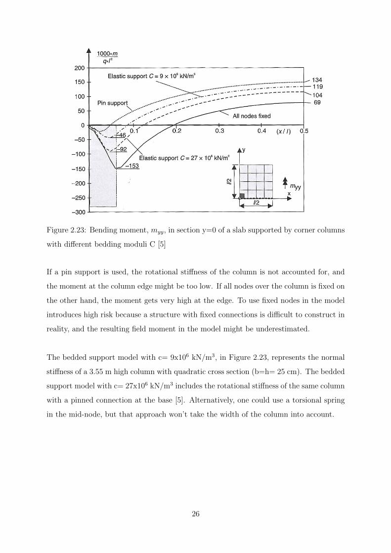
Figure 2.23: Bending moment, myy, in section y=0 of a slab supported by corner columns

with different bedding moduli C [5]

If a pin support is used, the rotational stiffness of the column is not accounted for, and

the moment at the column edge might be too low. If all nodes over the column is fixed on

the other hand, the moment gets very high at the edge. To use fixed nodes in the model

introduces high risk because a structure with fixed connections is difficult to construct in

reality, and the resulting field moment in the model might be underestimated.

The bedded support model with c= 9x106 kN/m3, in Figure 2.23, represents the normal

stiffness of a 3.55 m high column with quadratic cross section (b=h= 25 cm). The bedded

support model with c= 27x106 kN/m3 includes the rotational stiffness of the same column

with a pinned connection at the base [5]. Alternatively, one could use a torsional spring

in the mid-node, but that approach won’t take the width of the column into account.

26

The most precise results are achieved when the rotational stiffness of the columns is

accounted for. It is, however, both difficult and time-consuming to determine the correct

stiffness, and hence it might be more economical to use a conservative simplification.

Another possibility is to model the edge and corner columns in the same way as monolithic

connections where the entire column is included in the model [6]. However, as for the

rotational stiffness, it might be beneficial to use a conservative simplification.

2.6 Modelling of load conditions

The loads in a FEM-analysis are always defined as point loads in the nodes. Even if the

FEM software package allows the user to model an arbitrary load arrangement, the load

will be automatically replaced by nodal loads. Nodal loads may in general be obtained by

load lumping, or as work-equivalent consistent nodal loads. Load lumping is a term used

for distributed loads getting discretized to the nearest nodes so that the nodal forces are

statically equivalent to the applied force; however, load lumping should be restricted to

linear elements with only corner nodes, otherwise it gives erroneous results [4].

Work-equivalent (consistent) nodal loads are also statically equivalent to applied load;

furthermore, the work done by the nodal forces on the nodal displacements, equals the

work done by the applied load over the entire displacement field. The consistent nodal

loads are obtained by use of the same shape functions as was used for calculating the

stiffness matrix. These methods won’t be discussed in further details here, but it is

important to be aware of the fact that uniformly distributed loads always get distributed

to the nodes [4].

It is also worth noticing that many software packages neglect the load on restrained

nodes since that load is transferred straight to the support without affecting the rest of

the structure. Hence, the total support force is the sum of the forces on the unrestrained

nodes only. It is important to be aware of this fact when the results for a structure

component are used as loading for another structure component [4].

27

2.7 Singularities

Singularities are caused by simplifications in the numerical models. By assuming linear-elastic

behaviour in disturbed regions, where the material in reality is highly non-linear, one

achieves infinitely high stresses, which do not occur in real life. Typical regions of

singularities are:

• Walls that end within a slab

• Discontinuous line supports

• Pin support

• Obtuse corners

• Openings

• Re-entrant corners (α ≥ 90◦)

• Concentrated loads

In singularity zones, the stress will get higher with increasing fine mesh, as illustrated in

Figure 2.24 for a simply supported slab (1x1 m) subjected to a point load of 1000 kN in

the centre.

Figure 2.24: Stresses in a plate for element sizes 0.5 m (left) and 0.02 m (right) when

subjected to a concentrated load (modelled in ”FEM design”)

28

In Figure 2.25, some typical singularity regions are marked in a typical building floor.

As discussed in section 2.5 (about support conditions), singularities due to walls ending

within a slab can be solved by either ignoring the missing support and design a fully

restrained beam in the opening, or inserting bedded nodes at the edge of the support.

Singularities due to pin supports, can be removed either by replacing the support with

surface loading or by replacing the pin support with springs connected to a stiff plate

which can rotate around the support point. However, it should be noted that it is usually

unnecessary to remove singularities over supports, as the design forces can be found from

critical sections outside the support centre [5].

Figure 2.25: Singularity regions [5]

In re-entrant corners of an opening, singularities will arise because of inconsistency of the

forces around the corners. While the bending moment on top and bottom of the opening

approaches zero, the bending moment along the sides of the opening is non-zero, and

hence there will be a jump in the moments at the corners, see Figure 2.26. This can be

solved by rounding the corners in the model [5].

29

Figure 2.26: Moment distribution of my in sections near the corner of an opening

(modelled with ”DIANA”)

When two walls meet in a re-entrant corner with an angle α ≥ 90◦, as shown in Figure 2.27,

the singularity can be clearly seen upon mesh refinement. The plate is simply supported

and subjected to a uniformly distributed load of 10 kN/m2. The coarse mesh to the left

has a stress value in the re-entrant corner of 6950 kN/m2, while the fine mesh to the right

has a stress of 8910 kN/m2, which is an increase of almost 30%. Further refinement of

the mesh would produce stresses approaching infinity. The singularity can be avoided by

including the stiffness of the walls in the model. This is shown in Figure 2.28, where the

two sides, which makes up the re-entrant corner, are bedded instead of simply supported.

When these supports are given a vertical stiffness of 1e+04 kN/m/m, the singularity is

avoided at the cost of a slightly greater field moment.

Figure 2.27: Stresses in a re-entrant corner for an element size of 2m (left) and 0.25m

(right) (modelled with ”DIANA”)

30

Figure 2.28: Bending moment, mxx [kNm/m], in a plate with a re-entrant corner (modelled

with ”FEM design”)

Singularities due to point loads can be avoided by dispersing the load down to the

mid-plane of the slab, and hence get a greater loaded width in the analysis as illustrated

in Figure 2.29 [5].

Figure 2.29: Dispersion of concentrated loads

31

2.8 Mesh refinement

The FEM programs available today are capable of dividing the structure into an almost

infinite number of elements, but it’s at the cost of longer computational time. The field

moments are rarely affected by the mesh fineness, and there’s no point in using more

elements than necessary. However, in regions close to concentrated loads or supports, the

results highly depend on the mesh fineness; the more elements, the better results. This

can be seen, in Figure 2.30, for a simply supported one-way slab with two equal spans of

5 m and a uniformly distributed load. The field moments are almost independent of the

mesh fineness, while the support moment deviates significantly when different number of

elements are used. The shear force over the supports is also different for different number

of elements, but since the design forces are found outside of the support, the result is

rarely affected by the mesh [5].

32

Figure 2.30: Member forces of a one-way slab for different numbers of finite elements [5]

The required number of elements are dependent on the polynomial order of the shape

functions. When first order polynomials are used instead of second order polynomials,

more elements are normally needed. This is illustrated in Figure 2.31, which compares

axial deformation and axial stress for a 1D bar, of length 3×l, with various number of

elements and polynomial order. It can be seen that one quadratic element performs better

than one linear element, but three linear elements give almost correct deformation. It’s

also worth noticing that the deformations are generally more accurate than the stresses,

because the stresses are derived from the deformations [4].

33

Figure 2.31: Axial deformation and axial stress for a 1D bar with elements of different

polynomial order [4]

There are actually some exceptions to the claim that more elements always give better

results. In singularity regions, as discussed in Section 2.7, the stresses increase to unrealistic

levels when the mesh is (unreasonably) refined. However, even in singularity zones, the

mesh should be fine enough to sufficiently model the forces at the support edge, where

the design forces are found. In regions with high stress gradients, the maximum stress in

the element can be greater than the stresses found from the integration points; therefore,

the resulting design might become unsafe [5].

If the moment distribution found in the critical sections is smeared out in the perpendicular

direction, as illustrated with dashed lines in Figure 2.32, the influence of the mesh density

on the averaged moment is small. This is illustrated in Figure 2.33, where a plate

with dimensions 20m x 10m x 0.6m, supported by four inner columns, is subjected to

a uniformly distributed load of 10 kN/m2. The distribution of the moment, mxx, in the

section above the two columns on the right-hand side is shown for three different meshes.

The coarsest mesh is called 100%, and it can easily be seen that with a finer mesh the peak

value increases. However, the moment integrated over the area of the section is almost

34

equal for the three different meshes [3]. If an average moment is used for the design, it is

therefore sufficient to use two second order elements or one first order element from the

centre of the support to the critical section [6].

Figure 2.32: Smearing of moment peak [3]

Figure 2.33: Moment distribution for different mesh fineness [3]

Most FEM software packages available today offer to automatically discretize the structure

given an approximate size of the elements. However, in regions of great stress gradients

or concentrated loads, the structural engineer has to manually insert a sufficient number

of elements. It is also important to ensure that the nodes at the boundaries have been

positioned accurately, especially at curved boundaries. Even a very small deviation from

the correct coordinates can be critical. Curved boundaries will in general require a higher

number of elements in order to model the real deformation and load-bearing behaviour

[5]. It is also important to ensure that no elements cross interfaces. If, for example, there

is a change in material, nodes should be placed along the interface line [15].

35

2.9 Choice of control sections

As mentioned previously, when modelling in single points or along a discrete line, the

assumption of a linear-elastic material is a simplification that will produce too high values

for the forces and moments. In reality, the concrete will crack and the reinforcement will

yield, and the maximum values, which are used for design, are actually found in the result

sections outside of the support centre. The exact location of the result sections will first

be discussed for moments, and then for shear forces.

2.9.1 Result sections for moments

The location of the result section depends on the stiffness of the connection. For monolithic

connections, the critical bending crack will develop no closer to the support than on the

support edge, and hence it is safe to use the support surface as the result section. This is

in accordance with the recommendation in EC2 5.3.2.2 [8]. Figure 2.34 shows the location

of the result section for bending moment in a monolithic connection, where the width,

”a”, represents the length of a rectangular cross-section. In the case of a circular column

with a diameter of φ, the equivalent value of ”a” can be found from Eq. 2.5 [6].

aeqv =

√πφ

2(2.5)

Figure 2.34: Result section for bending moment in a monolithic connection [6]

If the connection is hinged, and the support only transfers compression stresses, the

location of the result section is dependent on the stiffness of the support. If the support is

36

stiff, the resultant force on each half side will be approximately at the support edge. If, on

the other hand, the support is soft, the stress over the support will be almost uniformly

distributed, which gives resultant forces at the middle of each half, see Figure 2.35 for an

illustration of this. The stiffer the support, the more the resultant force will shift towards

the edge. A column support will always shift the resultant force more towards the edge

than a wall support. The result section of a simply supported slab can, as a conservative

assumption, always be taken as the mid-section in between the centre and the edge of

the support. This is applicable for walls, columns and bearings in agreement with EC2

5.3.2.2 [6, 8]. EC2 5.3.2.2 states that support moments, which are calculated with a span

from centre to centre of supports, can be reduced with ∆M as shown in Eq. 2.6. This

corresponds to shifting the resultant section a/4 out of the centre when the support load

is uniformly distributed [8].

∆M =FEd,supa

8(2.6)

Figure 2.35: Result sections for bending moment in a hinged connection with a stiff

support (left) and a soft support (right) [6]

37

2.9.2 Result sections for shear forces

Shear forces in a plate are due to the vertical forces which are transferred from the plate

towards the supports. The result section for shear forces should be placed where the

critical shear crack develops, which is where the crack can transfer the largest possible

shear force. This will be no closer to the support than at the edge, because if it is any

closer, the vertical force is transferred directly to the support. Hence, the critical result

section should be placed at a distance of z×cotθ from the support edge, where z is the

internal lever arm and θ is the crack angle as illustrated in Figure 2.36. Without shear

reinforcement, the crack angle will be steeper than 45◦, and z×cotθ is approximately equal

to the effective height of the slab, d. When controlling shear compression failure, the full

shear force at the support edge should be used [6].

Figure 2.36: Result section for shear force [6]

38

2.10 Stress smoothing

As mentioned previously, the stresses in an element are found in integration points where

the stresses are most accurate. However, it is desired to have the same accuracy for the

stresses in the entire element, and to achieve this one can use element smoothing. Element

smoothing involves extrapolating the element stresses from the integration points, σhs , to

the rest of the element by use of the same set of shape functions, Nu, which were used to

determine the displacement field. This can be seen in Eq. (2.7), where σ∗ is the smoothed

stress field [4]. An example on how an element smoothed stress field may look like is

shown in Figure 2.37. It can be seen that the smoothed stress field looks relatively similar

to the real stress field because of the smoothing of the discrete FEM stresses [4].

σ∗ = Nuσhs (2.7)

Figure 2.37: Element stress field σ (left), and element smoothed stress field σ∗ (right) [4]

Even though element smoothing gives a continuous stress field inside the element, the

stresses are still discontinuous over element borders. Unless there actually is a discontinuity

in geometry or material in the structure, the stresses should be continuous over the element

borders. This can be done by using nodal averaging, where the nodal stress becomes the

average of the original nodal stresses in each of the surrounding elements. The nodal

stress from each element is found either directly or by extrapolating from the integration

points. When the averaged nodal stresses are found, continuity across element borders

is achieved, and continuous stress field for each element can be found by interpolating

the nodal average stresses with the use of the shape functions, Nu. This can be seen in

Eq. (2.8), where σ∗n is a vector with the nodal stress averages in the element. [4].

σ∗ = Nuσ∗n (2.8)

39

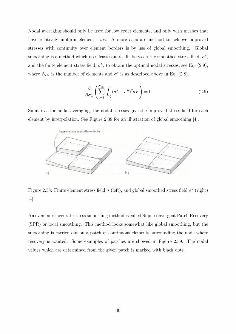
Nodal averaging should only be used for low order elements, and only with meshes that

have relatively uniform element sizes. A more accurate method to achieve improved

stresses with continuity over element borders is by use of global smoothing. Global

smoothing is a method which uses least-squares fit between the smoothed stress field, σ∗,

and the finite element stress field, σh, to obtain the optimal nodal stresses, see Eq. (2.9),

where Nels is the number of elements and σ∗ is as described above in Eq. (2.8).

∂

∂σ∗n

(Nels∑e=1

∫Ve

(σ∗ − σh)2dV

)= 0 (2.9)

Similar as for nodal averaging, the nodal stresses give the improved stress field for each

element by interpolation. See Figure 2.38 for an illustration of global smoothing [4].

Figure 2.38: Finite element stress field σ (left), and global smoothed stress field σ∗ (right)

[4]

An even more accurate stress smoothing method is called Superconvergent Patch Recovery

(SPR) or local smoothing. This method looks somewhat like global smoothing, but the

smoothing is carried out on a patch of continuous elements surrounding the node where

recovery is wanted. Some examples of patches are showed in Figure 2.39. The nodal

values which are determined from the given patch is marked with black dots.

40

Figure 2.39: Examples of patches for lower and higher order elements [4]

The least-square fit method as described in Eq. (2.9) is still used, but the smoothed

stress field, σ∗, is now described by a vector, P, which contains polynomial terms in the

Cartesian coordinates, and a vector, a, containing unknown generalized coordinates for

which the derivation should be solved with regard to, see Eq (2.10):

σ∗ = Pa (2.10)

The summation inside the least-square fit is done over the number of sampling points in

the patch, and not over the number of elements as in global smoothing. when a is found,

the smoothed nodal values can be found with equation Eq. (2.10) where the Cartesian

coordinates of the nodes are inserted in P. Since the elements often are included in

more than one patch, a unique solution for the stress field in an element can be found by

multiplying the shape function for a node with the recovered stress found from SPR in

that node, see Eq. (2.11), where Nen is the number of element nodes [4].

σ∗ =Nen∑a=1

Naσ∗a (2.11)

41

The user of a FEM design software should be conscious of what coordinate system is used

to report the element stresses, what type of integration points is used, what techniques

the program uses to extrapolate and interpolate, and what method is used for stress

averaging. If all this is known, the user is more likely to interpret the output from the

analysis correct. It might be useful to avoid stress smoothing, because the degree of stress

discontinuity gives information about the accuracy of the finite element results [4].

All programs for FEM design use the stress resultants from the analysis as input in the

design. The stress resultants are obtained by integrating the stresses over the thickness

of the plate, see Eqs. (2.12)-(2.14), and Figure 2.40.

mx = −∫ t

2

− t2

σxzdz (2.12)

my = −∫ t

2

− t2

σyzdz (2.13)

mxy = −∫ t

2

− t2

τxyzdz (2.14)

42

Figure 2.40: Stresses (top) and stress resultants (bottom) in a bending plate

43

44

Chapter 3

Design of plates

3.1 General

In this chapter, the theory of elasticity and the sandwich model will be described as they

are the basis for numerous design programs.

The main difficulty with both these models are the fact that in general, plates don’t have

coinciding principal moment- and reinforcement directions. In beam theory, the principal

moment always works in the load bearing direction. Plates on the other hand, have

load bearing in two directions, and twisting moments that disturb the principal moment

directions. It is almost impossible to place the reinforcement in the directions of the

principal moments, because the directions may vary over the plate; moreover, a plate

normally experience various load cases during a lifetime, which gives principal moments

in varying directions.

45

3.2 Design based on theory of elasticity

The theory of elasticity is based on the equilibrium equation of an infinitesimal plate

element subjected to distributed load in the normal direction, see Figure 3.1. Mx and My

are bending moments, Mxy and Myx are equal torsion moments, and Vx and Vy are shear

forces.

Figure 3.1: Forces in an infinitesimal plate element [7]

From equilibrium of the forces in the element, the result is Eq. (3.1) [7].

δ2Mx

δx2+δ2Mxy

δxδy+δ2My

δy2= −q (3.1)

This equation holds for all infinitesimal plate elements. In the theory of elasticity,

however, it is further assumed that the material is linear-elastic and isotropic, the vertical

deformation is small compared to the thickness of the plate, Kirchhoff’s theory is valid, and

that there is plane stress in the xy-plane. By use of these assumptions in the constitutive

and kinematic relations, the results are Eqs. (3.2)-(3.4), where w represents the vertical

deformations, and D is the plate flexural stiffness.

46

Mx = −D(∂2w

∂x2+ ν

∂2w

∂y2

)(3.2)

My = −D(∂2w

∂y2+ ν

∂2w

∂x2

)(3.3)

Mxy = − ∂2w

∂x∂yD(1− ν) (3.4)

When Eq. (3.2)-(3.4) are inserted into Eq. (3.1), the fourth order partial differential

equation for elastic bending of isotropic plates is achieved [7]:

∂4w

∂x4+ 2

∂4w

∂x2∂y2+∂4w

∂y4=

q

D(3.5)

This equation can be solved analytically as long as the plate is rectangular and has ideal

boundary conditions. Several tables with results for moments and deflections exists for

different span ratios, boundary conditions, and Poisson’s ratios [7].

When the design moments are found, the next step in the design of a concrete plate is

to calculate the moment capacity of the compression zone, which is done with moment

equilibrium according to Eq. (3.6), where α is the relative height of the compression zone

[16]:

MRd = 0, 8α(1− 0.4α)fcdbd2 (3.6)

Then, an approximation of the internal lever arm can be found dependent on the compression

zone utilization according to Eq. (3.7) [16]:

z =

(1− 0.17

MEd

MRd

)dx ≤ 0.95d (3.7)

47

Finally, the required reinforcement for the Ultimate Limit State (ULS) can be found

according to Eq (3.8):

As =MEd

z × fyd(3.8)

This procedure is performed for each reinforcement direction independently. If torsion

moment is present, the required cross section area of anchoring reinforcement is:

Aanchoring =2Mxy

fyd(3.9)

For the Serviceability Limit State (SLS), the vertical deformation, w, is found from tables.

Reduced bending stiffness should be used due to cracking of concrete.

3.3 The sandwich model

One widely used model for calculating the required reinforcement is the sandwich model.

The sandwich model method is a general procedure for design of shells, but it is also

applicable for plates since the only difference between plates and shells is that shells

include membrane forces.

The first step in the sandwich model method is to divide the plate into three layers, and

then translating the stress resultants into in-plane forces in the layers. The shear forces

are handled by the middle layer, and the outer layers handle the bending moments and

in-plane forces. The outer layers also help support the middle layer. The thickness of the

outer layers depend on whether the concrete is cracked or not. If the concrete is cracked,

the thickness of the layer is assumed to be two times the distance from the surface to

the reinforcement gravity centre. If the concrete is uncracked the thickness of the layer is

assumed to be half the plate thickness. When the thickness of the top and bottom layer

is found, the middle layer is simply the remaining thickness of the plate. In bending,

we assume cracked concrete as a conservative approach because it gives the largest lever

arm, and hence the highest utilization of the reinforcement. Figure 3.2 illustrates the

imaginary in-plane forces in the three layers of a sandwich model [7].

48

Figure 3.2: The layers of a sandwich model for a shell element [7]

The second step in the sandwich model method is to control whether shear reinforcement

is necessary or not. This is done by finding the principal shear force, v0, and the associated

shear angle, ϕ0, according to Eqs. (3.10) and (3.11), and control that v0 is smaller than

the shear compressive capacity and the shear tensile capacity which both are given in

EC2, chapter 6 [7].

v0 =√v2x + v2y (3.10)

ϕ0 = tan−1(vyvx

)(3.11)

49

If the shear capacity is insufficient, shear reinforcement is needed, and can be calculated

using EC2. By adding shear reinforcement, there will be extra contributions to the

in-plane forces in the outer layers with a value of ∆n, see Eqs. (3.12)-(3.14). Cotθ is

the angle to the compression strut in the concrete (see Figure 3.3), and can be chosen

between 1< cotθ <2.5 [7].

∆nx =1

2

v2xv0cotθ (3.12)

∆ny =1

2

v2yv0cotθ (3.13)

∆nxy =1

2

vxvyv0

cotθ (3.14)

Figure 3.3: Compression struts and the angle θ [8]

In the third step, the total value of the in-plane forces in the top and bottom layers are

calculated. It is assumed orthogonal reinforcement in the directions corresponding to the

local axis. The contributions from the internal moments are simply the moment divided

by the internal lever arm which goes from the middle of the top layer to the middle of the

bottom layer. In the next step, the maximum principal in-plane force in each of the outer

layers is calculated according to Eq. (3.15). This is done to control whether the concrete

is cracked or not [7].

n11 =nx + nynxy

+

√(nx − nynxy

)2

+ n2xy (3.15)

If the principal force, n11, is below zero, the concrete is uncracked; hence, minimum

reinforcement is sufficient as long as the compression stress is below the design compressive

50

strength, fcd. If the concrete is cracked, however, the design of the layer is done according

to compression field theory (CFT). CFT implies that there is equilibrium between the

fictitious in-plane forces, and the reinforcement- and compression strut forces. The

equilibrium conditions of the theory are illustrated in Figure 3.4 [7].

Figure 3.4: Equilibrium conditions in the compression field theory

The resulting expressions for the reinforcement forces in each direction, Fsx and Fsy, as

well as the concrete compression force, Fc are all shown in Eqs. (3.16)-(3.18) [7].

Fc =nxy

sinφcosφ(3.16)

Fsx = nx + nxytanφ (3.17)

Fsy = ny + nxycotφ (3.18)

51

The compression force has to be checked against the dimensioning maximum compression

stress, σRd,max, from EC2 6.5.2, see Eq (3.19):

σRd,max = 0.6

(1− fck

250

)fcd (3.19)

The concrete compression capacity is reduced compared to pure compression capacity, fcd,

due to the effect of the transverse tensile stress. In the theory of elasticity, this reduction

in capacity is neglected since each direction is calculated independently.

If the compression capacity is insufficient, there are several possibilities to solve the

problem. Three options are illustrated in Figure 3.5 [7].

a) Account for the compression capacity in the reinforcement

b) Increase the concrete cover locally

c) Increase the thickness of the layer

Figure 3.5: Different ways to solve a problem of too low concrete compression capacity

[7]

Alternative a) might lead to buckling of the reinforcement, and hence a brittle failure

mode which is undesirable. Alternative b) is not a practical approach at the building site.

The most practical option is alternative c) where the thickness of the layer is increased

while the reinforcement stays at its original position. In that case, the forces due to the

eccentricity have to be recalculated [7].

52

Finally, the required reinforcement amount is found from Eqs. (3.20) and (3.21), where

fyd is the yield strength of the reinforcement [7].

Asx =Fsxfyd

(3.20)

Asy =Fsyfyd

(3.21)

This is a quick and simple method, but it has some disadvantages. It assumes constant

stress and strain in the outer layers, which is inaccurate, and cracking is only controlled

in the mid-plane of the membrane [7].

53

54

Chapter 4

Commercial FEM design software

4.1 Introduction

This chapter will show some examples on how automatic design of concrete plates can

be done with reference to some of the commercial design software packages available today.

In all of the automatic procedures for design described in this thesis, it is assumed that

the concrete only supports compressive forces, while the reinforcement supports all the

tensile forces.

Some of the programs offer both calculation of necessary reinforcement, and capacity

control for applied reinforcement. A description of how the design and/or control is done

for both Ultimate Limit State (ULS) and Serviceability Limit State (SLS) is included for

each of the selected software packages. Due to variable access to the theory behind the

calculations, the focus for each software package will be different.

The notations in this chapter changes for each subsection in order to use the same notation

as in the given programs.

55

4.2 Design with ”FEM design”

4.2.1 Ultimate limit state (ULS)

The ”FEM design” software package from StruSoft is an advanced design tool for concrete,

steel, and timber. The primary source of information for this chapter is ”FEM-Design,

Applied Theory and Design” [9].

When deciding the mesh density, one should be aware of the fact that ”FEM design” only

uses Mindlin plates. If the plate is thin, the mesh near edges needs to be very fine to

capture the effect of the decreasing twisting moment. It is also worth noticing that ”FEM

design” uses an average value for the nodal forces between elements of the same kind.

This is done to avoid discontinuities generated from the FEM calculation. The ”FEM

design” theory background does, unfortunately, not document what method is used for

the stress smoothing.

”FEM design” can calculate the necessary reinforcement in either the whole structure or

in selected parts. It is also possible to manually edit the reinforcement lay-out by deleting

or adding reinforcement bars, and then let the program calculate utilization factors for

the bars. The reinforcement bars can be placed in two arbitrary directions, and they

don’t have to be perpendicular to each other. The directions of the reinforcement are

called ξ and η, and the angles between the reinforcement directions and the global x-axis

are called α and β, respectively. The various directions and angles are shown in Figure

4.1 [9].

Figure 4.1: Coordinate system in ”FEM design” [9]

56

The first step of the automatic design procedure is to translate the moments from the

x-y coordinate system to the ξ-ϑ coordinate system, with the use of the rotation matrix,

Rα, see Eq.(4.1). The results are the formulas given in Eqs. (4.2) - (4.4). Notice that the

ϑ-direction is perpendicular to the ξ-direction, and not necessarily equal to the second

reinforcement direction, η [9].

M ′ξϑ = RαMRT

α

M ′ξϑ =

mξ mξϑ

mξϑ mϑ

, Rα =

cosα sinα

−sinα cosα

,M =

mxx mxy

mxy myy

(4.1)

mξ =mx +my

2+mx −my

2cos2α +mxysin2α (4.2)

mϑ =mx +my

2− mx −my

2cos2α−mxysin2α (4.3)

mξϑ = −mx −my

2sin2α +mxycos2α (4.4)

Secondly, the moments are rotated to the ξ-η-coordinate system by use of the Rϕ matrix,

see Eq. (4.5).

M ′ξη = RϕM

′ξϑR

Tϕ

M ′ξη =

mξ mξη

mξη mη

, Rϕ =

sinϕ −cosϕ

0 1

, (4.5)

When the moments in the reinforcement directions are found, the program calculates

four cases of possible design moment pairs, which are called case a), b), ξ), and η).

Reinforcement in both directions are needed in the cases a) and b), and the design

moments are basically just the moments perpendicular to the reinforcement axes, see

Figure 4.2. These design moments can be written as Eqs. (4.6) and (4.7), where x’ and

y’ represent the reinforcement directions (ξ and η).

57

m′1 = m′xx ±m′xy (4.6)

m′2 = m′yy ±m′xy (4.7)

Figure 4.2: Design moments normal to the reinforcement directions [10]

In Cases ξ) and η) on the other hand, one of the reinforcement moments are set to zero

because only reinforcement in one direction is needed. The other reinforcement moment

is found from optimal reinforcement amount consideration.

The four cases as they are written in ”FEM design”, with respect to moments in the

ξ-ϑ-coordinate system, are listed in Eqs. (4.8)-(4.15). A case is valid if the signs of mξ

and mη are equal, and mη + mξ > mx + my. If a valid moment pair is positive, then these

are the design moments for the bottom reinforcement. If, however, the valid moment pair

is negative, these moments should be used for design of the top reinforcement.

Case a)

mξ = mξ −mϑcosϕ

1 + cosϕ+mξϑ

1− 2 cosϕ

sinϕ(4.8)

mη = mϑ1

1 + cosϕ+mξϑ

1

sinϕ(4.9)

Case b)

mξ = mξ +mϑcosϕ

1− cosϕ−mξϑ

1 + 2 cosϕ

sinϕ(4.10)

mη = mϑ1

1− cosϕ−mξϑ

1

sinϕ(4.11)

58

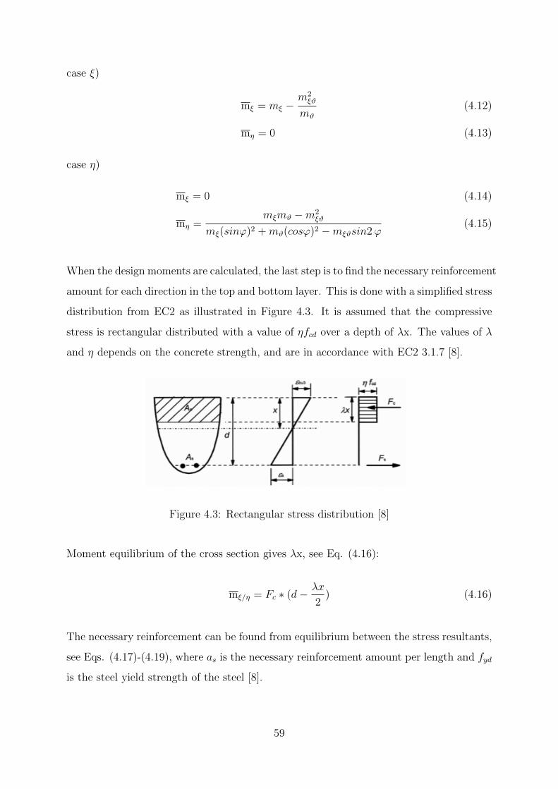
case ξ)

mξ = mξ −m2ξϑ

mϑ

(4.12)

mη = 0 (4.13)

case η)

mξ = 0 (4.14)

mη =mξmϑ −m2

ξϑ

mξ(sinϕ)2 +mϑ(cosϕ)2 −mξϑsin2ϕ(4.15)

When the design moments are calculated, the last step is to find the necessary reinforcement

amount for each direction in the top and bottom layer. This is done with a simplified stress

distribution from EC2 as illustrated in Figure 4.3. It is assumed that the compressive

stress is rectangular distributed with a value of ηfcd over a depth of λx. The values of λ

and η depends on the concrete strength, and are in accordance with EC2 3.1.7 [8].

Figure 4.3: Rectangular stress distribution [8]

Moment equilibrium of the cross section gives λx, see Eq. (4.16):

mξ/η = Fc ∗ (d− λx

2) (4.16)

The necessary reinforcement can be found from equilibrium between the stress resultants,

see Eqs. (4.17)-(4.19), where as is the necessary reinforcement amount per length and fyd

is the steel yield strength of the steel [8].

59

Fc = Fs (4.17)

λx ∗ η ∗ fcd = as ∗ fyd (4.18)

as =λx ∗ η ∗ fcd

fyd(4.19)

The result can be displayed like in Figure 4.4. The figure shows the required reinforcement

in mm2/m for a quadratic plate with sides equal to 10 m, and thickness of 0.2 m. The

plate is simply supported on all edges, and has a uniformly distributed surface load of

10 kN/m. The element borders are shown with blue lines, and the nodes are illustrated

with circles. It can be seen that ”FEM design” uses 9-node plate elements in this case,

but 6-node triangular elements are also available for bending plates.

Figure 4.4: Example of design output from ”FEM design” [mm2/m]

The ”FEM design” software supports peak smoothing over singularity regions. this means

that the program calculates an average moment over a chosen distribution region. Figure

4.5 shows how smoothing over a column peak can look like in the program.

60

Figure 4.5: Example of peak smoothing with ”FEM design”

4.2.2 Serviceability Limit State (SLS)

”FEM design” can perform crack- and deflection control of the structure. This is done

according to EC2 7.3.4 and 7.4.3, respectively [8]. The user can do the control assuming

either cracked or uncracked concrete. If the concrete is uncracked, the full stiffness of the

structure will be used. If the concrete is cracked, however, the stiffness will be reduced

to somewhere in between the stiffness of an uncracked and fully cracked structure. The

correct stiffness is found by iterations according to the workflow illustrated in Figure 4.6

until the deflection from two consecutive calculations differ with less than a chosen

percentage, or the maximum allowed number of iterations is reached. The calculations are

based on either the applied or the required reinforcement. If it is based on the required

reinforcement, the reinforcement in each element is the maximum required reinforcement

calculated from all load cases.

61

Figure 4.6: The workflow of the stiffness iteration in ”FEM design”

4.2.3 Verification

In order to verify the automatic design method in ”FEM design”, a plate element subjected

to constant moments are designed both by hand, and in the program. The input parameters

are:

Concrete C30/37

h = 200 mm

fcd = 17 MPa

Es = 200 GPa

fyd = 434.8 MPa

Ø = 10 mm (reinforcement diameter)

62

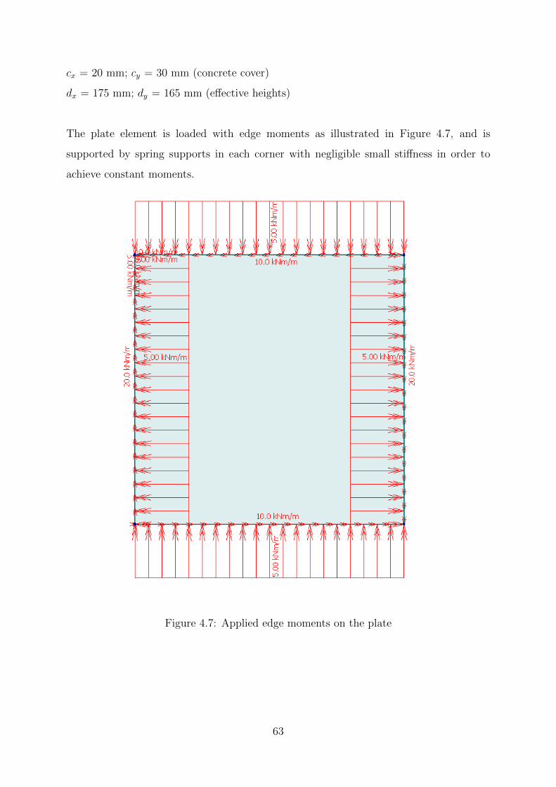
cx = 20 mm; cy = 30 mm (concrete cover)

dx = 175 mm; dy = 165 mm (effective heights)

The plate element is loaded with edge moments as illustrated in Figure 4.7, and is

supported by spring supports in each corner with negligible small stiffness in order to

achieve constant moments.

Figure 4.7: Applied edge moments on the plate

63

For orthogonal reinforcement where ξ corresponds with the global x-direction, and η

corresponds with the y-direction (ϕ=90◦):

mx = mξ = 20 kNm/m (4.20)

my = mϑ = mη = −10 kNm/m (4.21)

mxy = mξϑ = mξη = 5kNm/m (4.22)

The four possible design moment pairs are then:

Case a)

mξ = mξ −mϑcosϕ

1 + cosϕ+mξϑ

1− 2 cosϕ

sinϕ= mξ +mξϑ = 25 kNm/m (4.23)

mη = mϑ1

1 + cosϕ+mξϑ

1

sinϕ= mϑ +mξϑ = −5 kNm/m (4.24)

Case b)

mξ = mξ +mϑcosϕ

1− cosϕ−mξϑ

1 + 2 cosϕ

sinϕ= mξ −mξϑ = 15 kNm/m (4.25)

mη = mϑ1

1− cosϕ−mξϑ

1

sinϕ= mϑ −mξϑ = −15kNm/m (4.26)

Case ξ)

mξ = mξ −m2ξϑ

mϑ

= 22.5 kNm/m (4.27)

mη = 0 (4.28)

Case η)

mξ = 0 (4.29)

mη =mξmϑ −m2

ξϑ

mξ(sinϕ)2 +mϑ(cosϕ)2 −mξϑsin2ϕ=mξmϑ −m2

ξϑ

mξ

= −11.25 kNm/m (4.30)

The cases a) and b) are invalid solutions because mη and mξ have different signs. Cases

ξ) and η) on the other hand, are valid solutions, because the signs are equal, and mη+mξ

64

≥ mx+my. Case ξ) will be used to calculate the bottom reinforcement since the moment

is positive, and case η) will be used to calculate the top reinforcement. An overview of

the design moments are shown in Figure 4.8.

Figure 4.8: The design moments for hyperbolic bending with orthogonal reinforcement

[kNm/m]

Calculation of the required bottom reinforcement in the ξ-direction:

mξ = fcd × λx(d− λx

2) (4.31)

22500Nmm

mm= 17

N

mm2× λx(175mm− λx

2) (4.32)

λx = 7.73mm (4.33)

asξ =λx× η ∗ ×fcd

fyd(4.34)

asξ =7.73mm× 1.0× 17N/mm2

434.8N/mm2(4.35)

asξ = 0.3022mm2/mm = 302.2mm2/m (4.36)

65

The top reinforcement in the η-direction is calculated in the same way, and gives asη =

158.7mm2/m, see Eqs (4.37)-(4.40). Figure 4.9 shows the required reinforcement results

from ”FEM design” which correlates very well with the values calculated by hand. The

small deviations are due to rounding errors.

11250Nmm

mm= 17

N

mm2× λx(165mm− λx

2) (4.37)

λx = 4.06mm (4.38)

asη =4.06mm× 1.0× 17N/mm2

434.8N/mm2(4.39)

asη = 0.1587mm2/mm = 158.7mm2/m (4.40)

Figure 4.9: The required reinforcement for hyperbolic bending with orthogonal

reinforcement in ”FEM design” [mm2/m]

If the reinforcement is non-orthogonal, the calculation will appear slightly different than

for the orthogonal case. Even though it is unpractical to use non-orthogonal reinforcement,

it might be necessary because of the geometry of the structure. Therefore, a new verification

is done for an angle of ϑ = 75◦ between ξ and η, where ξ corresponds with the global

x-axis, as illustrated in Figure 4.10. The moment input is as shown in Eqs. (4.41)-(4.43).

66

mx = mξ = 20 kNm/m (4.41)

my = mϑ = −10 kNm/m (4.42)

mxy = mξϑ = 5 kNm/m (4.43)

Figure 4.10: Coordinate-system for calculation with non-orthogonal reinforcement

The four possible design moment pairs are then:

Case a)

mξ = mξ −mϑcos(75◦)

1 + cos(75◦)+mξϑ

1− 2 cos(75◦)

sin(75◦)= 24.55 kNm/m (4.44)

mη = mϑ1

1 + cos(75◦)+mξϑ

1

sin(75◦)= −2.76 kNm/m (4.45)

Case b)

mξ = mξ +mϑcos(75◦)

1− cos(75◦)−mξϑ

1 + 2 cos(75◦)

sin(75◦)= 8.65 kNm/m (4.46)

mη = mϑ1

1− cos(75◦)−mξϑ

1

sin(75◦)= −18.67 kNm/m (4.47)

Case ξ)

mξ = mξ −m2ξϑ

mϑ

= 22.5 kNm/m (4.48)

mη = 0 (4.49)

67

Case η)

mξ = 0 (4.50)

mη =mξmϑ −m2

ξϑ

mξ(sin2(75◦)) +mϑ(cos2(75◦))−mξϑsin(2× 75◦)= −14.53 kNm/m (4.51)

The cases a) and b) are, as discussed earlier, not valid because the signs of the moment

pairs are unequal. Case ξ) will give the same amount of required bottom reinforcement

as for the previous example with orthogonal reinforcement (asξ = 302.2mm2/m). The

top reinforcement, however, has to be re-calculated:

mη = fcd × λx(d− λx

2) (4.52)

14530Nmm

mm= 17

N

mm2× λx(165mm− λx

2) (4.53)

λx = 5.26mm (4.54)

asη =λx× η × fcd

fyd(4.55)

asη =5.26mm× 1.0× 17N/mm2

434.8N/mm2(4.56)

asη = 0.2057mm2/mm = 205.7mm2/m (4.57)

The required reinforcement calculated in ”FEM design” is shown in Figure 4.11, and the

small deviation from the values calculated by hand are only due to rounding errors.

68

Figure 4.11: The required reinforcement for hyperbolic bending with non-orthogonal

reinforcement [mm2/m]

The top-reinforcement is increased with almost 30% compared to the solution with orthogonal

reinforcement. This is due to the fact that the reinforcement direction, η, is further away

from the principal moment direction. The directions of the principal moments are shown

in Figure 4.12; it is rotated 9.2◦ anticlockwise relative to the global coordinate system,

see Eq. (4.58).

α0 = arctan

(m1 −mx

mxy

)= arctan

(20.81− 20

5

)= 9.2◦ (4.58)

Figure 4.12: The principal moments in the plate [kNm/m]

69

4.3 Design with ”Robot Structural Analysis Professional”

4.3.1 Ultimate Limit State (ULS)

”Robot Structural Analysis Professional” (”Robot”) is a program from Autodesk. ”Robot”

supports analysis and design of several different structure components, including concrete

slabs. Most of the information presented in this chapter has been found in Robot’s ”User’s

Guide” [11].

For plane elements in bending state, discrete Kirchhoff-Mindlin triangles or quadrilaterals

are used with a one or four point Gaussian quadrature, respectively. Similar to Mindlin

plate elements, these elements include shear strain fields. However, contrary to Mindlin

elements, they prevent the problem with shear locking for thin plates [17].

The internal forces can be displayed with either global smoothing, local smoothing,

averaged values in element centres or without any stress smoothing. How the stresses

from the integration points are extrapolated to the nodes is unclear in the ”User’s Guide”.

”Robot” has three different methods for determining required reinforcement in plates and

shells:

• Analytical method

• Equivalent moment method (Wood & Armer) [18]

• Equivalent moment method according to the Netherlands Standardization Institute

(NEN)

The NEN- and the Wood & Armer method are both simplified methods which enable

faster calculations, and normally sufficiently accurate results for plates in pure bending

or bending with only small membrane forces. For shell structures with both bending and

membrane forces, the analytical method must be used. Because these scenarios are not

relevant for this thesis, it won’t be described further.

The workflow of the Wood & Armer method is showed in Figure 4.13, where x and y are

the chosen directions of the reinforcement.

70

Figure 4.13: Dimensioning of slabs according to Wood & Armer

A positive moment gives tension at the bottom of the plate, while a negative moment

gives tension at the top. The formulas for design moments are found from the compression

field theory described for the sandwich model method in Section 3.3, see Eqs.(4.59) and

(4.60).

71

M∗xd = Mx + |Mxy| tan θ (4.59)

M∗yd = My + |Mxy| cot θ (4.60)

If the design momentM∗xd ≥ 0, the angle to the compression strut in the concrete, θ, can be

assumed to be ±π4, which gives the minimum total amount of reinforcement. If, however,

the design moment M∗xd ≤ 0, there is no tension at the bottom in the x-direction, so M∗

xd is

set to zero. The design moment in the y-direction should therefore be recalculated with a

new θ for optimal reinforcement amount. This is found by inserting M∗xd=0 in Eq. (4.59),

resulting in cotθ = Mxy/|Mx|, and then use this in Eq (4.60). The same procedure is

followed for the y-direction [11].

Correspondingly, if the design moment M∗xg ≥ 0, there is no tension at the top of the

plate in the x-direction, and M∗xg is set to zero, while M∗

yg is recalculated with a new θ

[11]. When the reinforcement is orthogonal, this method equals the method from ”FEM

design”. Another commonality is the fact that the internal lever arm is found by assuming

a rectangular stress distribution in the cross section.

The NEN method is a simplification of the Wood & Armer method, where it is assumed

that the compression strut angle always is ±π4. Hence, the design moments are simply

given as in Eqs. (4.61) and (4.62) for both the upper and lower reinforcement [11].

M∗x = Mx ± |Mxy| (4.61)

M∗y = My ± |Mxy| (4.62)

If this method is used, the required reinforcement amount increases compared to the

Wood & Armer method. This can be illustrated with the same example as was used in

the verification of the ”FEM design” program where a plate element was loaded with

constant moments, and given orthogonal reinforcement:

72

mx = 20kNm/m (4.63)

my = −10kNm/m (4.64)

mxy = 5kNm/m (4.65)

With the NEN-method, this results in a bottom reinforcement in the x-direction of 337.0

mm2/m, and an upper reinforcement in the y-direction of 212.7 mm2/m, see Eqs. (4.66)-(4.79).

The increase in the reinforcement amount, is as much as 11% and 34%, respectively,

compared to the values from the more complex Wood & Armer method. The values for

the Wood & Armer method are the same as the values calculated in Section 4.2.3 for

”FEM design”.

M∗xd = 20 + 5 = 25 kNm/m (lower) (4.66)

M∗yg = −10− 5 = −15 kNm/m (upper) (4.67)

M∗xd = fcd × λx(d− λx

2) (4.68)

25000Nmm

mm= 17

N

mm2× λx(175mm− λx

2) (4.69)

λx = 8.62mm (4.70)

asx =λx× η × fcd

fyd(4.71)

asx =8.62mm× 1.0× 17N/mm2

434.8N/mm2(4.72)

asx = 0.3370mm2/mm = 337.0mm2/m (4.73)

M∗yg = fcd × λx(d− λx

2) (4.74)

15000Nmm

mm= 17

N

mm2× λx(165mm− λx

2) (4.75)

λx = 5.44mm (4.76)

73

asy =λx× η × fcd

fyd(4.77)

asy =5.44mm× 1.0× 17N/mm2

434.8N/mm2(4.78)

asy = 0.2127mm2/mm = 212.7mm2/m (4.79)

4.3.2 Serviceability Limit State (SLS)

The SLS deformation calculation in ”Robot” is based on the elastic deformation, but it

is linearly scaled to compensate for cracking and applied reinforcement, see Eqs. (4.80)

and (4.81) [11].

uiR = ui ∗ DB

(4.80)

D = E ∗ 1[m] ∗ h3

12(4.81)

uiR: The real displacement in point i in the plate

ui: The elastic displacement in point i

D: Elastic stiffness of the plate

B: Equivalent stiffness of the reinforced slab

The equivalent stiffness, B, is an averaged value of the equivalent stiffness in each reinforcement

direction, Bx and By. The averaging is done according to Eq. (4.82) [11].

Bix,y = cf ∗Bx + (1− cf ) ∗By (4.82)

The coefficient, cf , is a weight coefficient which depends on the moment ratio, and is

calculated according to Eq. (4.83). If the ratio between the moments in the two directions

of the reinforcement is more than four, the equivalent stiffness in the direction of the

greatest moment will be decisive.

74

cf = 1, 0

cf = 0, 5 +2

3∗ |Mxx| − |Myy|max(|Mxx|; |Myy|)

cf = 0, 0

for|Mxx||Myy|

> 4

for 0.25 ≤ |Mxx||Myy|

≤ 4

for|Mxx||Myy|

< 0.25

(4.83)

The next step is to calculate the average stiffness ratio, D/B, by using the formula shown

below, where B(Mmax) is the equivalent stiffness of the element containing the maximum

moment in any direction.

D

B= 0, 25 ∗

(D

Bixy

)+ 0, 75 ∗

(D

B(Mmax)

)(4.84)

The equivalent stiffness (elastic) method, described above, averages the stiffness for all

finite elements, so that the whole plate is assigned the same stiffness. The resulting

deflection is therefore the elastic deflection times the average stiffness ratio, as illustrated

in the left part of Figure 4.14. However, if a method with stiffness update is used (inelastic

method), the stiffness is calculated independently for each element and each direction,

resulting in an anisotropic plate of varying rigidity, as illustrated to the right of Figure 4.14

[11].

Figure 4.14: Left: Stiffness averaged for all elements. Right: Different stiffness for all

elements [11]

75

The crack control in ”Robot” is done by direct calculation of the crack width, according

to Eurocode 2, based on the equivalent moments in the two reinforcement directions. For

both the crack calculation and the deflection calculation, ”Robot” offers to automatically

increase the tension reinforcement if the crack width or the deflection is too high [11].

4.4 Design with ”DIANA”

4.4.1 Ultimate Limit State (ULS)

”DIANA” (DIsplacement ANAlyzer) is a finite element software package, developed by

DIANA FEA BV, which is able to both find the required reinforcement, and to calculate

the utilization of the applied reinforcement. The reinforcement bars can be applied in

two directions which don’t necessarily have to be orthogonal. ”DIANA” can design both

thick and thin plates since both Kirchhoff and Mindlin plates are offered. The information

source for major parts of this chapter is ”DIANA User’s Manual” [10].

The first step of the plate design in ”DIANA” is to rotate the calculated internal forces,

mx, my, and mxy to the chosen direction of the reinforcement. This is done similarly to

what was described previously for ”FEM design” in Section 4.2.1.

Like in the sandwich model, ”DIANA” transforms the internal forces to in-plane forces in

a top- and a bottom layer. As discussed in Chapter 3.3, the sandwich model assumes the

layer thicknesses to be two times the concrete cover, and the lever arm to be the distance

between the midpoints. ”DIANA”, however, sets the lever arm as the effective depth of

the plate, d, times a relative lever arm, zr, as illustrated in Figure 4.15. The value of zr

depends on the ratio between the bending moments and the membrane forces, and is by

default set to 0.9 [10].

76

Figure 4.15: Different internal lever arms [7]

The next step is to calculate the reinforcement forces. This is similar to Fsx and Fsy

in the sandwich model, except for the fact that ”DIANA” assumes the crack angle to

always be 45◦ which normally gives the smallest amount of reinforcement. This method

is similar to the previously described NEN-method in Section 4.3.1, except for the fact

that ”DIANA” works with equivalent in-plane forces instead of design moments. The

reinforcement forces in ”DIANA” are called n′c1 and n

′c2 , and are given in Eqs. (4.85) and

(4.86) for the upper layer, and correspondingly for the bottom layer [10].

n′c1,up = n

′cxx,up + n

′cxy,up (= Fsx′) (4.85)

n′c2,up = n

′cyy,up + n

′cxy,up (= Fsy′) (4.86)

The required reinforcement per unit length is then calculated with Eqs. (4.87) and (4.88):

Areq,x =n

′c1

fyd(4.87)

Areq,y =n

′c2

fyd(4.88)

”DIANA” offers to check the utilization of applied reinforcement in the structure compared

to the required amount. In addition, ”DIANA” automatically does a unity check on

the applied reinforcement related to the maximum and minimum reinforcement areas

according to EC2.

77

Before the design check in ”DIANA”, the user has to specify the bar diameter and spacing

for the reinforcement in both directions. However, the stiffness off the reinforcement grid

is not accounted for as long as the grid is labelled for design check. If it is desired to

account for the stiffness, ”DIANA” either applies the reinforcement stiffness directly or

automatically calculates and applies the equivalent thickness for the reinforcement grids

[10].

Since the concrete compression capacity is reduced if a lateral tensile force is present,

”DIANA” has several model options to calculate the reduction factor. This thesis won’t

go into detail about the models, but some of the available options are mentioned below.

They all have in common that they depend on the cracking of the concrete due to the

lateral tensile force.

• No reduction of the compressive strength

• Model of Vecchio and Collins 1993 [19]

• Model of Japan Society of Civil Engineers (JSCE) 2012 [20]

• Model with a multi-linear diagram

The shear capacity is controlled by calculating the principal shear force, referred to as q’

in ”DIANA”, with Eq.(4.89). As long as q’ is smaller than the shear compressive capacity

and the shear tensile capacity, given in EC2 chapter 6, the capacity is sufficient [10].

q′ =√q2x + q2y (4.89)

After the analysis are performed in ”DIANA”, there are many output options for the

various results. Even though the results may look different with different output options,

they are all based on the same results from the integration points. The available ways of

displaying the stress, strain, etc. are listed below [10]:

• Constant per reinforcement (uses the maximum integration point value inside the

grid)

• Constant per element (uses the maximum integration point value inside the element)

78

• Different for every integration point

• Extrapolated from the integration points to the nodes of the element

• Averaged in the direction normal to the reinforcement bars over a user defined

length, which is related to the thickness of the plate. The average results over the

reinforcement particles that are intersected by this line are calculated and displayed

in the integration points.

4.4.2 Serviceability Limit State (SLS)

Since reinforced concrete is a non-linear material, but linear-elastic analysis is preferable,

”DIANA” has an iterative method for calculating load distributions, deformations, crack

patterns, and crack openings in the structure. The first step in the procedure is to

calculate the stress distribution for an initial Young’s modulus and a Poisson’s ratio.

The program then controls whether the stresses at all integration points are below a

user-specified uniaxial stress-strain curve. If that is not the case, the concrete will crack,

and the local stiffness will be reduced. This is illustrated in Figure 4.16, where the stress

σ0 is outside the stress-strain curve, and the stiffness is therefore changed from E0 to E1.

The stress distribution is then re-calculated, and new stresses are found at the integration

points. This procedure is repeated until all stresses are inside the curve, or the maximum

allowable number of iterations is reached. The stiffness adaption analysis can be performed

for various number of load steps. With large load increments, many integration points

will reach too high stresses, and a widely spread area will obtain reduced stiffness. With

small load increments, however, the cracks will be much more localized [10].

79

Figure 4.16: Uniaxial stress-strain curve with stress and stiffness reduction [10]

Whereas ”FEM design” and ”Robot” perform the crack control by direct calculation

of the crack width, ”DIANA” controls cracking without direct calculations, but instead

restricts the bar diameter and spacing according to tabulated values in EC2 7.3.3. This is

a simplified control used for slabs in buildings subjected to bending with limited tension,

and overall thickness ≤200 mm. In order to use the simplified control, the requirements

for minimum reinforcement and the structural rules for plates, given in EC2 9.3, should

be fulfilled [8].

4.4.3 Verification

In order to verify the design procedure in ”DIANA”, the same example with a plate

element subjected to a constant moment as was used for ”FEM design” will be used here.

Since ”DIANA” has defined that positive moments give tension in the top of the plate,

the bending moments have opposite signs of the ”FEM design” example:

m′

xx = −20 kNm/m (4.90)

m′

yy = 10 kNm/m (4.91)

m′

xy = 5 kNm/m (4.92)

80

It is used an average value for the effective height in the x- and the y-direction, so that

the internal lever arm, for both directions, is:

zd = 0.9 ∗ d = 0.9 ∗ 170mm = 153mm (4.93)

The imaginary in-plane forces in the top layer of the plate is then:

n′

xx,up =m

′xx

zd=−20 ∗ 106Nmm/m

153mm= −130718.95N/m (4.94)

n′

yy,up =m

′yy

zd=

10 ∗ 106Nmm/m

153mm= 65359.48N/m (4.95)

n′

xy,up =

∣∣∣∣∣m′xy

zd

∣∣∣∣∣ =5 ∗ 106Nmm/m

153mm= 32679.74N/m (4.96)

The imaginary in-plane forces in the bottom layer of the plate will be equal, except that

the normal forces have opposite signs. Consequently, the design in-plane forces are:

n′c1,up = n

′cxx,up + n

′cxy,up = −98039.21N/m (4.97)

n′c1,low = n

′cxx,low + n

′cxy,low = 163398.69N/m (4.98)

n′c2,up = n

′cyy,up + n

′cxy,up = 98039.22N/m (4.99)

n′c2,low = n

′cyy,low + n

′cxy,low = −32679.74N/m (4.100)

Reinforcement is only required for positive values of the design forces. Consequently,

reinforcement is only needed in the x-direction in the bottom layer, and in the y-direction

in the top layer.

The calculated required reinforcement is then 375.8 mm2 in the bottom layer, and 225.5

mm2 in the top layer, see Eqs. (4.101) and (4.102):

Areq,x =n

′c1,low

fyd=

163398.69N/m

434.8MPa= 375.80mm2/m (4.101)

Areq,y =n

′c2,up

fyd=

98039.21N/m

434.8MPa= 225.48mm2/m (4.102)

81

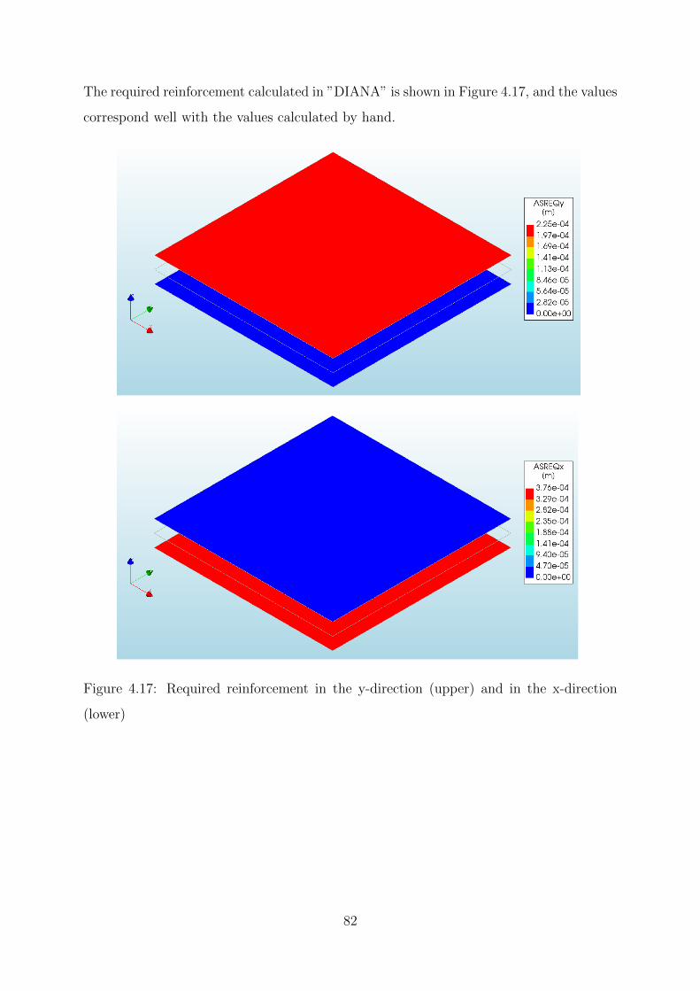
The required reinforcement calculated in ”DIANA” is shown in Figure 4.17, and the values

correspond well with the values calculated by hand.

Figure 4.17: Required reinforcement in the y-direction (upper) and in the x-direction

(lower)

82

4.5 Design with ”SOFiSTiK”

4.5.1 Ultimate Limit State (ULS)

The software ”SOFiSTiK” developed by SOFiSTiK AG offers several different FEM

packages which include all the necessary programs needed to analyse and design different

structures. The internal forces and moments are calculated with the program ”ASE-General

Static Analysis of Finite Element Structures” (ASE). ASE makes use of Mindlin theory

in plate calculations. The program used for design is called ”BEMESS”, and it is the

focus of this chapter. Most of the information is found in the manual ”BEMESS- Design

of Plates and Shells” [12].

”BEMESS” distinguishes between three different design cases:

• Disks

• Plates

• Shells

If disk is chosen, the structure is designed as a disk, even though out-of-plane forces might

actually be present in the structure [12].

An orthogonal reinforcement grid is in most cases the most effective solution, but ”BEMESS”

also offers a two-course oblique reinforcement for slightly skew constructions, and three-course

oblique reinforcement for higher skewness than 60◦. A radial and a tangential orthogonal

reinforcement is available for circular plates [12].

The principals of the plate design are similar to that of ”DIANA”. The moments are

initially transformed to the direction of the applied or calculated reinforcement directions.

Then, the internal lever arm is determined from the compression zone utilization, as

illustrated in Figure 4.18. The more utilized the compression zone is, the smaller the lever

arm; however, it is unclear which formula ”BEMESS” uses in this calculation. The fictive

in-plane forces are calculated using the lever arm. Finally, the necessary reinforcement is

calculated according to the selected code [12].

83

Figure 4.18: Stress and strain distributions in the cross-sections [12]

In ”BEMESS”, the shell design is very similar to the sandwich model, and can also be used

for plate design. The plate thickness is divided into three layers, where the outer layers

are given a thickness of 35% each of the total thickness. The lever arm is, in contrast to

plate design, calculated assuming full utilization of the compressive zone. The average

concrete cover between the two reinforcement directions is applied as concrete cover. An

illustration of the different layers and the internal lever arm is shown in Figure 4.19.

Figure 4.19: Fictitious disks and lever arm for shells [12]

Secondly, the fictive in-plane forces are calculated as half the membrane forces summed

up with the moment forces divided by the lever arm, z. As the next step, the principal

forces in each layer are calculated together with the angle, α, between the principal forces

and the applied reinforcement directions. Then α is used to transform the in-plane forces

to equivalent forces in the direction of the reinforcement. The required amount of tensile

reinforcement is found by dividing the in-plane forces with fyd.

84

As the final step, the concrete compression is controlled. In the case of compressive stress

in the concrete together with transverse tensile stress, the compression capacity of the

concrete is reduced according to the chosen design code. If the concrete can’t resist the

principal compressive force alone, ”BEMESS” offers to apply compression reinforcement.

However, compression reinforcement is only allowed if the reinforcement directions at

the upper and lower side coincides. This is to guarantee that the full stiffness from

the reinforcement at the opposite side can be accounted for. If additional compressive

reinforcement is added, the internal lever arm should change due to a higher compression

zone; however, this is not automatically adapted in ”BEMESS” [12].

The shear control is performed by calculating the principal shear force, v0, and controlling

that it is less than the shear tension capacity, VRd,c, and the shear compression capacity

VRd,max, from EC2. If the design shear force v0 > VRd,c, the user can either add more

longitudinal reinforcement, or add shear reinforcement. In the latter case, the required

shear reinforcement, assuming perpendicular shear links, is calculated according to EC2

(or chosen code). The shear utilization degree determines the inclination, θ, of the fictive

compression struts which is needed in the shear design calculation.

4.5.2 Serviceability Limit State (SLS)

The first SLS check ”BEMESS” performs is a control of the minimum thickness of the

compression zone. This control is performed in the directions of the principal moments.

Since the calculation of the compression zone height requires that the reinforcement area

is in the given direction, the reinforcement area gets converted from its original position

to the principal direction. It is unclear in the User Manual why this test is performed.

”BEMESS” also offers to control the crack width, both with direct calculations, as

in ”FEM design”, and without direct calculations, as in ”DIANA”. It is, however,

recommended in the manual for ”BEMESS” to normally use the crack control without

direct calculations.

85

The SLS stresses, stress range, and fatigue can be controlled in three different ways

with different level of simplifications and modifications. The simplest version uses the

calculated internal forces directly without iterations. The more complex method finds

equilibrium between all the forces, mxx, myy, mxy, nxx, nyy, nxy, and the corresponding

six strains in an iterative way to assure mechanical consistency. The manual doesn’t get

into detail about each method; hence, this thesis won’t either.

86

Chapter 5

Simple beam example

5.1 Introduction

In order to show the difference between the different procedures in a simple way, a one

meter wide plate strip of length 10m is subjected to two equal and symmetric edge

moments, Mx=30 kNm. The plate strip is designed for ULS according to the different

methods that have been presented in this thesis. For simplicity, all load factors are set to

1.0. An illustration of the beam is shown in Figure 5.1.

The input parameters are:

Concrete C30/37

h = 200 mm

fcd = 17 MPa

Es = 200 GPa

fyd = 434.8 MPa

Ø = 10 mm (reinforcement diameter)

cx = 35 mm (concrete cover)

dx = 160 mm (effective height)

87

Figure 5.1: Simply supported slab subjected to edge moments, Mx. Side view (top) and

plan view (bottom)

5.2 Strain compatibility

The plate strip is initially designed using strain compatibility, which was explained in

Section 3.2 for design based on the theory of elasticity. The moment capacity of the

compression zone is calculated assuming normally reinforced cross section, see Eq. (5.1):

MRd = 0.275fcdbd2 = 0.275× 17MPa× 1000mm× (160mm)2 = 119.7 kNm (5.1)

As the next step, an approximate internal lever arm is calculated from the moment

capacity utilization, see Eq. (5.2), where the design moment, MEd, is equal to the edge

moment, Mx = 30 kNm.

z =

(1− 0.17

MEd

MRd

)d =

(1− 0.17

30kNm

119.7kNm

)160mm = 153.18mm (5.2)

Finally, the required reinforcement is found from moment equilibrium of the cross section:

As =MEd

z × fyd=

30× 106Nmm

153.8mm.8MPa= 450.4mm2 (5.3)

88

5.3 The sandwich model

If the plate strip is calculated with the sandwich model, and the thickness of the layers

are assumed to be two times the distance from the surface to the reinforcement centre,

the in-plane design force in the bottom layer will be:

Fsx = nx =mx

z=

mx

h− 2c(5.4)

Fsx =30 ∗ 106N/mm2

200mm− 2× 40mm= 250000.0N (5.5)

The required bottom reinforcement in the longitudinal direction will then be:

As =Fsxfyd

=250000.0N

434.8MPa= 575.0mm2 (5.6)

5.4 ”FEM design”

The input moments for design in ”FEM design” is as follows:

mx = mξ = 30 kNm/m (5.7)

my = mϕ = mη = 0 kNm/m (5.8)

mxy = mξϕ = mξη = 0 kNm/m (5.9)

The four possible design moment pairs are then given as shown in Eqs.(5.10)-(5.17):

Case a)

mξ = mξ −mϑcosϕ

1 + cosϕ+mξϑ

1− 2 cosϕ

sinϕ= mξ = 30 kNm/m (5.10)

mη = mϑ1

1 + cosϕ+mξϑ

1

sinϕ= 0 kNm/m (5.11)

Case b)

mξ = mξ +mϑcosϕ

1− cosϕ−mξϑ

1 + 2 cosϕ

sinϕ= mξ = 30 kNm/m (5.12)

mη = mϑ1

1− cosϕ−mξϑ

1

sinϕ= 0 kNm/m (5.13)

89

Case ξ)

mξ = mξ −m2ξϑ

mϑ

= 30 kNm/m (5.14)

mη = 0 (5.15)

Case η)

mξ = 0 (5.16)

mη =mξmϕ −m2

ξϕ

mξ(sinϕ)2 +mϕ(cosϕ)2 −mξϕsin2ϕ= 0 kNm/m (5.17)

It is clear that the only possible moment pair is mξ = 30 kNm and mη= 0 kNm, resulting

in reinforcement in the bottom of the plate.

The rest of the calculation of the required bottom reinforcement in ξ direction is shown

in Eqs. (5.18)-(5.23):

mξ = fcd × λx(d− λx

2) (5.18)

30000Nmm

mm= 17

N

mm2× λx(160mm− λx

2) (5.19)

λx = 11.44mm (5.20)

asξ =λx× η × fcd

fyd(5.21)

asξ =11.44mm× 1.0× 17N/mm2

434.8N/mm2(5.22)

asξ = 0.4473mm2/mm = 447.3mm2/m (5.23)

The results calculated by the program are shown in Figure 5.2, and correlates well with

the results calculated by hand.

Figure 5.2: Required reinforcement from ”FEM design”

90

5.5 ”Robot Structural Analysis”

Since the reinforcement is orthogonal, and the loading is very simple, both the NEN

method and the Wood&Armer method give the same design moment, m∗xd=30 kNm, in

the bottom. The stress distribution in the cross section, and hence the internal lever arm,

is similar to that of ”FEM-design”; consequently, the required bottom reinforcement in

the longitudinal direction is also identical.

5.6 ”DIANA”

The edge moment Mx=30 kNm gives an imaginary in-plane force of:

n′cxx,lo =

m′xx

z=

Mx

0.9d=

30 ∗ 106Nmm

0.9 ∗ 160mm= 208333.3N = n

′c1,lo (5.24)

This design force gives a required bottom reinforcement of:

Areq,x =n

′c1,low

fyd=

208333.3N

434.8N/mm2= 479.1mm2 (5.25)

The required reinforcement calculated by ”DIANA” is shown in Figure 5.3, and correlates

well with the hand calculated value.

Figure 5.3: Required reinforcement in the longitudinal direction, designed with ”DIANA”

91

5.7 Comparison of the different methods

The required amount of reinforcement for the different models and programs varies significantly.

The lowest amount of reinforcement (447.3 mm2) calculated by ”FEM design”, deviates

more than 20% from the sandwich model (575.0 mm2). The main reason for the difference

is that the models have different values for the internal lever arms. While ”FEM design”

calculates the internal lever arm with the least possible compression zone height (14.3

mm), the sandwich model assumes the compression zone to be 80 mm, with uniformly

distributed compression stress. In the sandwich model the compression stress can be lower

than the compression strength, while ”FEM design” assumes the compression zone to be

fully utilized.

”FEM design” and ”Robot” both assume a rectangular stress distribution according to

Eurocode 2. Since the models have no restrictions for the steel strain, it might turn out

to be very large, see Figure 5.4. With a compression zone height of x=14.3 mm, and

the ultimate concrete strain set to 3.5‰, the steel strain in the model will be as high

as 35.7‰. In reality, the compression stress would have been distributed over a longer

compression zone, and the steel strain would be lower.

Figure 5.4: Possible strain distribution with rectangular stress distribution

In a normally reinforced cross section, as shown in the example with strain compatibility,

the maximum allowed steel strain is 5‰. For ULS, the programs and EC2 have no direct

limit for the reinforcement strain. For SLS, however, the steel strain is restricted by the

maximum allowed deflection of the plate, because large strains give large deflection.

92

Chapter 6

Discussion and conclusion

This thesis has described and compared several different methods for the modelling and

design of concrete plates in finite-element programs. What is important to remember

is that the results produced by a program are never of a higher quality than the input

from the user (“garbage in – garbage out”). The structural engineer therefore needs to be

fully aware of the simplifications that have been made in the modelling process, and the

simplifications that have been made in the automatic design calculations in the program.

How the plate should be modelled depends on the given structure and loading, and

whether the purpose is to design a new structure or to reproduce a structure that already

exists. The parameters that varies are:

• The plate geometry

• The reinforcement directions

• The material parameters for both the concrete and the reinforcement

• The boundary conditions

• The load cases

• The element type

• The mesh

• The stress smoothing method

93

The most convenient way of modelling supports is normally with pin supports because it

is easy, avoids unintended rotational restraints, and gives sufficiently accurate results in

the critical section. If, however, the rotational restraint, or the vertical flexibility from

the wall or column do have a significant effect on the stresses in the plate, for example

on the plate edge, a more complex model should be used. One option is to apply spring

supports, where the stiffness has to be carefully calculated. Another option is to simply

model the whole wall or column. It is also possible to model the elements over a support

as infinitely stiff in order to account for the rotational stiffness from the support. This

might, however, lead to too much restraint.

Since linear-elastic material behaviour is assumed, the superposition principle is valid,

but unreasonably high stresses may arise in regions where the concrete in reality acts

highly non-linear. Such singularity zones are found over column supports, in re-entrant

corners, in openings, and at points of concentrated loads. This is normally not a problem

since the design forces are found outside of the singularity zone. However, if the actual

stress behaviour is of interest, the singularities can often be solved with bedded supports

around the singularity.

The automatic design procedures in the different programs mentioned in this thesis have

many similarities. First the stress resultants are created and rotated to the directions of

the reinforcement. Then, the design moments or imaginary in-plane forces, are calculated.

Finally, the required reinforcement is found for the upper and lower plate layer. Whether

the program allows the user to apply two or three reinforcement directions varies, and it

also varies whether the program allows oblique reinforcement or only orthogonal.

An important difference between the programs is how the calculation procedures define

the crack angle. When reinforcement is needed in both directions, an angle of π4

gives a

minimum amount of required reinforcement and is therefore what most of the programs

use. If, however, reinforcement is necessary in only one direction, a crack angle of π4

is no

longer optimal, and some of the programs (i.e., ”FEM design” and ”Robot”) recalculate

the angle in order to minimize the required reinforcement amount. With this approach,

the amount of reinforcement decreases compared to an analysis that keep the crack angle

94

constant at π4. To illustrate this, an example was done on a plate element subjected

to pure moments (mx= 20 kNm/m, my= -10 kNm/m, and mxy= 5 kNm/m) such that

only one reinforcement direction in each layer was necessary. The required reinforcement

was calculated according to both ”FEM design” and the NEN-method in ”Robot”. The

only important difference in the two methods is that while the NEN-method assumes the

crack angle to be π4, ”FEM design” calculates the optimal crack angle to minimize the

reinforcement. The increase in reinforcement amount, for a crack angle of π4

compared

to an optimal crack angle, for the lower and upper plate layer, was as much as 11% and

34%, respectively. It should be noted that a crack angle that gives a minimum amount of

reinforcement isn’t necessarily desired if the first cracks develop in an angle far from the

design crack angle. The rotation of the crack in such situations involve large deformation;

hence, the cracks become large.

Another difference that highly influences the results is the difference in internal lever arms

which affects the efficiency of the reinforcement. A longer internal lever arm will give a

more efficient reinforcement. If rectangular stress distribution is assumed (as in ”FEM

design” and ”Robot”), a long internal lever arm is possible, provided the compression zone

is very small. If a simply supported, 200 mm high beam is subjected to an edge moment

of 30 kNm, the internal lever arm is 154.3 mm (assuming rectangular stress distribution).

If, however, the steel strain is limited to a maximum value of 5‰, the internal lever arm is

153.2 mm. In ”DIANA”, the lever arm is the effective height, d, multiplied by a relative

compression zone height of 0.9 (as default). Applied to the beam example, ”DIANA”

gives a lever arm of 144.0 mm. The shortest lever arm (140 mm) is obtained with the

sandwich model assuming cracked concrete in the outer layers. In the beam example, the

lowest lever arm gives about 20 % more reinforcement than the longest one. Figure 6.1

gives an overview of the different stress distributions, and the internal lever arms that

are used by the different models. All of the models from the commercial software have in

common that there is no direct limit for the reinforcement strain for the Ultimate Limit

State (ULS). The deflection criteria in the Serviceability Limit State (SLS) will, however,

limit the steel strain. Which of the models that give the most accurate results depend on

the loading and the real compression stress distribution for each case.

95

Figure 6.1: Different models for stress distribution give different internal lever arms

In SLS it is important to account for the cracking of concrete. This is done either by

changing the stiffness locally for elements with too high stresses, or changing the stiffness

of the entire plate in order to obtain a smooth displacement field. The crack width control

is done with one of the following two methods:

• Direct calculation: The actual crack width is calculated, and controlled against the

maximum allowed value from the design code

• Indirect calculation: The reinforcement diameter and spacing is controlled according

to maximum values from tables in the design code.

While direct calculation gives more accurate results, indirect calculation saves computational

time, and is usually a sufficiently accurate estimate.

96

Bibliography

[1] Concrete bridge - Lutjegast (Holland). http://www.bartels-global.com/

projects/concrete-bridge-lutjegast-holland. [Online; accessed 29.04.2017].

[2] http://en.grupogic.mx/precast-concrete-slabs/. [Online; accessed

23.05.2017].

[3] Blaauwendraad, J. Plates and FEM: Surprises and Pitfalls. Springer, 2010.

[4] Mathisen, K.M. Lecture notes from the course ”The Finite Element Method

Introduction and Fundamental Concepts” at NTNU, 2015.

[5] Rombach, G.A. Finite-element Design of conrete structures. Practical problems and

their solutions. ICE Publishing, second edition, 2004.

[6] Pacoste, C., Plos, M., and Johansson, M. Recommendations for finite element

analysis for the design of reinforced concrete slabs. Technical report, KTH Royal

Institute of Tchnology, 2012. 52.

[7] Engen, M. Lecture notes from the course ”Concrete structures 3” at NTNU , 2016.

[8] EN 1992-1-1 Eurocode 2: Design of concrete structures - Part 1-1: General rules and

rules for buildings, Brussels, 2004. CEN.

[9] FEM-Design, Applied Theory and Design. http://download.strusoft.com/

FEM-Design/inst110x/theory.pdf. [Online; accessed 13.03.2017].

[10] DIANA - Finite Element Analysis User’s Manual release 10.1 Theory . https:

//dianafea.com/manuals/d101/Diana.html. [Online; accessed 15.03.2017].

97

[11] User’s guide-robot structural analysis professional software.

http://help.autodesk.com/view/RSAPRO/2017/ENU/?guid=

GUID-FF347447-519A-4A03-B3DC-2CDB5A6BE028. [Online; accessed 05.04.2017].

[12] SOFiSTiK AG. BEMESS-Design of Plates and Shells, SOFiSTiK 2016, 2016.

[13] Hughes, T.J.R. The Finite Element Method. Englewood Cliffs, 1987.

[14] Nielsen, M.P. and Hoang, L.C. Limit Analysis and Concrete Plasticity. CRC Press,

third edition, 2011.

[15] FEM Modeling: Mesh, Loads and BCs. http://www.colorado.edu/

engineering/CAS/courses.d/IFEM.d/IFEM.Ch07.d/IFEM.Ch07.pdf. [Online;

accessed 07.03.2017].

[16] Øverli, J.A. Formula sheet from the course ”Concrete structures 1” at NTNU , 2015.

[17] Katili, I. A new discrete kirchhoff-mindlin element based on mindlin–reissner

plate theory and assumed shear strain fields—part ii: An extended dkq element

for thick-plate bending analysis. International Journal for Numerical Methods in

Engineering, 136, 1993.

[18] Wood, R.H. The reinforcement of slabs in accordance with a pre-determined field of

moments. Garston, Eng. : Building Research Station, 1968.

[19] Vecchio, F. J. and Collins, M. P. . Compression response of cracked reinforced

concrete. Journal of Structural Engineering, 119, 1993.

[20] JSCE. Standard specifications for concrete structures - 2012 ”design”. Technical

report, Japan Society of Civil Engineers, 2012.

98

Appendices

99

Appendix A

Design with ”DIANA”

In 2016, ”DIANA” introduced ”DIANA Interactive Environment” (”DIANA IE”), a new

graphical user interface where it is possible to do the modelling, design, and post-processing

without programming. Because the program is relatively new, there is limited information,

forums and tutorials online, and few colleagues to ask. This appendix is therefore going

to describe the main steps for performing the design of a simple beam/plate strip. The

same plate strip as was used in the example in Chapter 5 will be used here.

First, the geometry of the beam is defined, and assigned material and geometrical properties.

This includes defining the element type, which should be set to Q20SH for design analysis.

The Q20SH element, shown in Figure 1.1, is a four-node quadrilateral isoparametric

curved shell element [10].

Figure 1.1: Q20SH element [10]

After the concrete beam is assigned properties, the reinforcement layers should be defined

with the same corner coordinates as the beam, but with z-coordinates corresponding

to the height of the top- and bottom reinforcement layer. For a beam in bending,

one reinforcement layer is sufficient, but for the sake of illustration, both the top- and

101

bottom layer is included here. When the layers are assigned reinforcement properties, it is

important that both the element geometry, and the material property for the reinforcement

is marked for design as illustrated in Figure 1.2; otherwise, the design check analysis is

unable to run.

Figure 1.2: Material and geometrical properties for the reinforcement

After this, the geometry tool bar at the left side of the display window should look like

Figure 1.3- 1.5.

Figure 1.3: The geometry tool bar: Geometry

102

Figure 1.4: The geometry tool bar: Materials

Figure 1.5: The geometry tool bar: Element geometries

The loads, supports, and units can be defined straight forward, and the geometry tool

bar should look like Figure 1.6-1.8. The final model can be seen in Figure 1.9.

103

Figure 1.6: The geometry tool bar: Loads

Figure 1.7: The geometry tool bar: Supports

104

Figure 1.8: The geometry tool bar: Reference systems

Figure 1.9: Final model of the simple beam

The model is now ready for the analysis. First, a new analysis has to be created. Then,

the commands ”Structural Linear Static”, and ”Design check” have to be selected, as

illustrated in Figure 1.10.

105

Figure 1.10: Add a new analysis

The final step is to define the required reinforcement as output for the design check. In

the properties for the output, a load set and a limit state needs to be defined. This is

illustrated in Figure 1.11- 1.13.

Figure 1.11: Add a new output

106

Figure 1.12: Edit properties of the output

Figure 1.13: Output properties

When ”DIANA 10.1” was used in this master thesis, the software failed to export some

of the commands, like the units-table, from the ”DIANA IE” to the actual code, so it had

to be inserted manually. The final code for the model is therefore attached below:

107

: Diana Datafile written by Diana 10.1'UNITS' LENGTH M MASS KG FORCE N TEMPER CELSIU ANGLE RAD'DIRECTIONS' 1 1.00000E+00 0.00000E+00 0.00000E+00 2 0.00000E+00 1.00000E+00 0.00000E+00 3 0.00000E+00 0.00000E+00 1.00000E+00'MODEL' GRAVDI 3 GRAVAC -9.81000E+00'COORDINATES' 1 1.00000E+01 1.00000E+00 0.00000E+00 2 1.00000E+01 0.00000E+00 0.00000E+00 3 0.00000E+00 0.00000E+00 0.00000E+00 4 0.00000E+00 1.00000E+00 0.00000E+00 5 1.00000E+00 0.00000E+00 0.00000E+00 6 2.00000E+00 0.00000E+00 0.00000E+00 7 3.00000E+00 0.00000E+00 0.00000E+00 8 4.00000E+00 0.00000E+00 0.00000E+00 9 5.00000E+00 0.00000E+00 0.00000E+00 10 6.00000E+00 0.00000E+00 0.00000E+00 11 7.00000E+00 0.00000E+00 0.00000E+00 12 8.00000E+00 0.00000E+00 0.00000E+00 13 9.00000E+00 0.00000E+00 0.00000E+00 14 9.00000E+00 1.00000E+00 0.00000E+00 15 8.00000E+00 1.00000E+00 0.00000E+00 16 7.00000E+00 1.00000E+00 0.00000E+00 17 6.00000E+00 1.00000E+00 0.00000E+00 18 5.00000E+00 1.00000E+00 0.00000E+00 19 4.00000E+00 1.00000E+00 0.00000E+00 20 3.00000E+00 1.00000E+00 0.00000E+00 21 2.00000E+00 1.00000E+00 0.00000E+00 22 1.00000E+00 1.00000E+00 0.00000E+00 23 1.00000E+01 1.00000E+00 6.00000E-02 24 1.00000E+01 0.00000E+00 6.00000E-02 25 0.00000E+00 0.00000E+00 6.00000E-02 26 0.00000E+00 1.00000E+00 6.00000E-02 27 1.00000E+01 1.00000E+00 -6.00000E-02 28 1.00000E+01 0.00000E+00 -6.00000E-02 29 0.00000E+00 0.00000E+00 -6.00000E-02 30 0.00000E+00 1.00000E+00 -6.00000E-02'MATERI' 1 NAME "concrete" MCNAME CONCDC MATMDL EN1992 ASPECT TOTCRK CONCRE EN1992 WEIGCC NORMAL CLASS "C30/37" AGGTYP QUARTZ

108

CEMTYP N CRACKN PLASTN TOTCRK ROTATE TENCRV BRITTL COMCRV EC2 POIRED DAMAGE YOUN28 3.28366E+10 POISON 2.00000E-01 THERMX 1.00000E-05 DENSIT 2.40000E+03 TENSTR 2.89647E+06 COMSTR 3.80000E+07 2 NAME "steel" MCNAME REINFO MATMDL LINEAR YOUNG 2.10000E+11 ASPECT DESIGN YLDSTR 4.34800E+08'GEOMET' 1 NAME "thickness" GCNAME SHEET GEOMDL FLASHL KFAC 1.50000E+00 XAXIS 1.00000E+00 0.00000E+00 0.00000E+00 THICK 2.00000E-01 2 NAME "diameterandspacing" GCNAME RSHEET GEOMDL REGRID XAXIS 1.00000E+00 0.00000E+00 0.00000E+00 DESIGN PHI 1.00000E-02 1.00000E-02 SPACIN 1.50000E-01 1.50000E-01 ZR 9.00000E-01'DATA' 1 NAME "Element data 1"'ELEMENTS' SET "Plate" CONNECT 1 Q20SH 2 1 14 13 2 Q20SH 13 14 15 12 3 Q20SH 12 15 16 11 4 Q20SH 11 16 17 10 5 Q20SH 10 17 18 9 6 Q20SH 9 18 19 8 7 Q20SH 8 19 20 7 8 Q20SH 7 20 21 6 9 Q20SH 6 21 22 5 10 Q20SH 5 22 4 3 MATERIAL 1 GEOMETRY 1 DATA 1'REINFORCEMENTS' SET "Reinforcement top"

109

LOCATI 1 GRID PLANE 24 23 26 25 MATERIAL 2 GEOMETRY 2 DATA 1 SET "Reinforcement bottom" LOCATI 2 GRID PLANE 28 27 30 29 MATERIAL 2 GEOMETRY 2 DATA 1'LOADS' CASE 1 NAME "edgemoment" ELEMEN 10 EDGE ETA2 MOMENT 3.00000E+04 DIRECT 2 1 EDGE ETA1 MOMENT -3.00000E+04 DIRECT 2'SUPPOR' NAME "edge" / 1-4 / TR 3'END'

110