Conceptual Design of a 2 Tesla Superconducting Solenoid ...lss.fnal.gov/archive/tm/TM-1886.pdfFermi...

Fermi National Accelerator Laboratory

FE-TM-1886

Conceptual Design of a 2 Tesla Superconducting Solenoid for the Fermilab D0 Detector Upgrade

J. Brzezniak, R.W. Fast, K. Krempetz, A. Kristalinski, A. Lee, D. Markley, A. Mesin, S. Orr, R. Rucinski, S. Sakla, R.L. Schmitt, R.P. Smith, B. Squires, R.P. Stanek, A.M. Stefanik,

A. Visser, R. Wands and R. Yamada

Fermi National Accelerator Laboratory P.O. Box 500, Batauia, Illinois 60510

May 1994

e Operated by Universities Research Association Inc. under Cantmcf No. DE-ACM-76CH030W titi the United States Department of Enegy

Disclaimer

This report was prepared as a/r account ofwork .sponsored 6y ao agency ofthe United States Government. Neither the United States Gouerunm~t nor my agency thereof; nor any of their employees, makes any warranty, rq~ress or implied, or assumes any legal liability or responsibility for the accuracy, completeness, or usefulrws of any information, apparatus, product, orprocess disclosed, or represmts that its use would not infringe priuately owned rights. Reference herein to my specific ~onmercial product, process, or service by trade nan~e, trademark, mawfacturer, or otherwise, does not necessarily constitute or imply its endorsement, reconrnreudutioa, or fauorirlg 6y the United States Gouernment or any agency thereof: The views and opinio:as of authors expressed herein do not necessarily state or reflect those ofthe United St&es Goverrmrent or any agency thereof.

TABLE OF CONTENTS

1. INTRODUCTION

1.1 General Description of the Present DO Detector ............................... l-l

1.2 Upgrade Project of the D0 Detector .......................................... l-2

1.3 General Requirements for the Superconducting Solenoid ....................... l-2

2. COIL DESIGN

2.1 General Features .............................................................. 2-l

2.2 Conductor Selection ........................................................... 2-l

2.3 Winding Design ............................................................... 2-3

2.4 Conductor Joints ............................................................. 2-3

2.5 Winding Procedure ........................................................... 2-4

3. FIELD AND FORCE CALCULATIONS

3.1 2-Dimensional Field Calculations .............................................. 3-l

3.2 Detailed Field Calculations Near the Solenoid .................................. 3-l

3.3 Integrated Field Uniformity ................................................... 3-2

3.4 3-Dimensional Field Calculations .............................................. 3-2

3.5 Decentering Forces ............................................................ 3-3

3.6 Stress Calculations by ANSYS ................................................ 3-5

3.7 Anaiytic Hoop Stress Analysis ................................................. 3-6

3.8 Displacement of Solenoid and Support Cylinder ................................ 3-7

4. MAGNET CRYOSTAT

4.1 General . . . . . . . . . . . . . . . . . . . . . . . . . . . . . . . . . . . . . . . . . . . . . . . . . . . . . . . . . . . . . . . . . . . . . . . 4-l

C-l

4.2 Vacuum Vessel ................................................................ 4-l

4.3 Cold Mass Support System .................................................... 4-l

4.4 Alignment of the Coil ......................................................... 4-3

4.5 Coil Thermal Design and Cool Down Characteristics ........................... 4-3

4.6 Loss ofVacuum ............................................................... 4-5

4.7 Liquid Nitrogen Cooled Shields and Intercepts ................................. 4-6

4.8 Radial Clearance and Tolerances .............................................. 4-7

4.9 Assembling the Coil and Cryostat ............................................. 4-7

5. SERVICE CHIMNEY

5.1 General ....................................................................... 5-l

5.2 Routing ...................................................................... 5-l

5.3 Vacuum Jacket ............................................................... 5-2

5.4 Internal Contents ............................................................. 5-2

5.5 Thermal Movement and Stress ................................................ 5-3

5.6 Fabrication and Location of Field Break ....................................... 5-3

5.7 Heat Loads ................................................................... 5-4

5.8 Vacuum Pumping and Relief Capacity ......................................... 54

5.9 Magnet Cryostat Nozzle ....................................................... 5-5

6. CONTROL DEWAR

6.1 General ....................................................................... 6-l

6.2 Mounting and Access ......................................................... 6-l

6.3 Vacuum Jacket ............................................................... 6-2

6.4 Vapor Cooled Current Leads .................................................. 6-2

6.5 Liquid Helium Reservoir ...................................................... 6-2

c-2

6.6 Heat Loads ................................................................... 6-3

6.7 Loss ofVacuum ............................................................... 6-3

7. REFRIGERATION SYSTEM

7.1 GeneralRequirements ......................................................... 7-l

7.2 Building Requirements ........................................................ 7-l

7.3 Flow Diagram ................................................................ 7-2

7.4 Hardware Components ........................................................ 7-2

7.5 System Heat Loads and Capacity .............................................. 7-3

7.6 Refrigeration Control System .................................................. 7-3

8. VACUUM SYSTEM

8.1 General ....................................................................... 8-1

8.2 Insulating Vacuum ............................................................ 8-l

8.3 Electrical Feedthroughs and Guard Vacuum ................................... 8-2

9. CONTROL AND INSTRUMENTATION

9.1 Overview ..................................................................... 9-l

9.2 Existing PLC System ......................................................... 9-l

9.3 System Instrumentation ....................................................... 9-2

9.4 Upgraded PLC System ........................................................ 9-3

9.5 Quench Protection Monitor ................................................... 9-4

9.6 Control System Power ......................................................... 9-5

10. DC ENERGIZATION CIRCUIT

10.1 DC Current Regulated Power Supply . . . . . . . . . . . . . . . . . . . . . . . . . . . . . . . . . . . . . . . . . 10-l

10.2 Ripple Filter . . . . .._.......................................................... 10-2

c-3

10.3 Dump Switch and Protection Resistor ........................................ 10-2

10.4 Reversing Switch ............................................................ 10-3

10.5 Crowbar ..................................................................... 10-3

10.6 Water Cooled BUS ........................................................... 10-3

10.7 Quench Detection ............................................................ 10-4

10.8 Interlocks and Controls ...................................................... IO-5

11. QUENCH CALCULATIONS

11.1 Quench Codes ................................................................ 11-l

11.2 QuenchStudy ................................................................ 11-l

11.3 Varying the Protection Resistor ............................................... 11-2

11.4 Adiabatic Estimate of Conductor Maximum Temperature ..................... 11-2

11.5 Charging and Discharging the Solenoid ....................................... 11-3

11.6 Protecting the Magnet Buses ................................................. 11-7

12. MANUFACTURING TESTS

12.1 General ...................................................................... 12-1

12.2 ApprovalofDesign ........................................................... 12-l

12.3 Mandatory Testing of Components ........................................... 12-2

12.4 Control Dewar and Chimney Tests at the Factory ............................. 1%?

12.5 Fully Integrated System Tests at the Factory ................................. 12-2

12.6 System Acceptance Tests at Fermilab ........................................ 12-2

12.7 Magnetic Field Mapping ..................................................... 12-3

13. OPERATION MODES

13.1 Steady State Operation . . . . . . . . . . . . . . . . . . . . . . . . . . . . . . . . . . . . . . . . . . . . . . . . . . . . . . 13-1

c-4

13.2 Non Steady State Operation ................................................. 13-1

13.3 Liquid Nitrogen System Operation ........................................... 13-2

14. APPENDIX A: SYSTEM PARAMETER TABLE ....................... A-l

15. APPENDIX B: FERMILAB SAFETY CONSIDERATIONS . . . ._. . . . B-l

16. APPENDIX C: APPLICABLE CODE REQUIREMENTS _. C-l

17. APPENDIX D: RADIATION AND INTERACTION LENGTHS . D-l

16. APPENDIX E: CONDUCTOR STABILITY

E.1 Conductor Stability ........................................................... E-l

E.2 Steady State and Transient Heating ........................................... E-l

E.3 The MPZ Theory ............................................................. E-2

E.4 Applying the MPZ Theory .................................................... E73

E.5 Conclusions .................................................................. E-4

19. APPENDIX F: ALIGNMENT CONSIDERATIONS

F.l General Remarks ............................................................. F-l

F.2 TeVatron Rquirements ........................................................ F-l

F.3 Tracking System Requirements ................................................ F-3

F.4 Vertex Resolution Due to Misalignment ....................................... F-4

20. APPENDIX G: SUPPORTING DOCUMENTS ......................... G-l

c-5

CHAPTER 1

INTRODUCTION

1.1 General Description of the Present D0 Detector

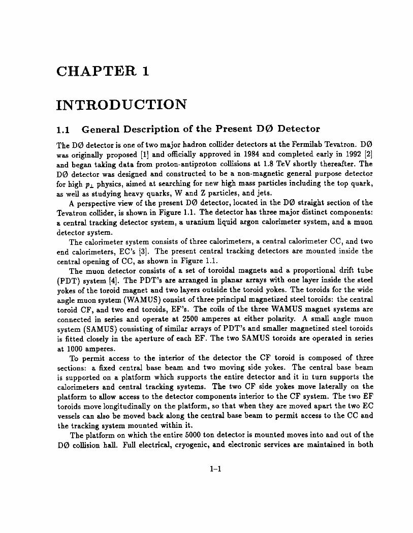
The D0 detector is one of two major hadron collider detectors at the Fermilab Tevatron. DO was originally proposed [l] and officially approved in 1984 and completed early in 1992 [2] and began taking data from proton-antiproton collisions at 1.8 TeV shortly thereafter. The DO detector was designed and constructed to be a non-magnetic general purpose detector for high pI physics, aimed at searching for new high mass particles including the top quark, as well as studying heavy quarks, W and Z particles, and jets.

A perspective view of the present DO detector, located in the D0 straight section of the Tevatron collider, is shown in Figure 1.1. The detector has three major distinct components: a central tracking detector system, a uranium liquid argon calorimeter system, and a muon detector system.

The calorimeter system consists of three calorimeters, a central calorimeter CC, and two end calorimeters, EC’s [3]. The present central tracking detectors are mounted inside the central opening of CC, as shown in Figure 1.1.

The muon detector consists of a set of toroidal magnets and a proportional drift tube (PDT) system [4]. The PDT’s are arranged in planar arrays with one layer inside the steel yokes of the toroid magnet and two layers outside the toroid yokes. The toroids for the wide angle muon system (WAMUS) consist of three principal magnetized steel toroids: the central toroid CF, and two end toroids, EF’s. The coils of the three WAMUS magnet systems are connected in series and operate at 2500 amperes at either polarity. A small angle muon system (SAMUS) consisting of similar arrays of PDT’s and smaller magnetized steel toroids is fitted closely in the aperture of each EF. The two SAMUS toroids are operated in series at 1000 amperes.

To permit access to the interior of the detector the CF toroid is composed of three sections: a fixed central base beam and two moving side yokes. The central base beam is supported on a platform which supports the entire detector and it in turn supports the calorimeters and central tracking systems. The two CF side yokes move laterally on the platform to allow access to the detector components interior to the CF system. The two EF toroids move longitudinally on the platform, so that when they are moved apart the two EC vessels can also be moved back along the central base beam to permit access to the CC and the tracking system mounted within it.

The platform on which the entire 5000 ton detector is mounted moves into and out of the DO collision hall. Full electrical, cryogenic, and electronic services are maintained in both

l-l

the assembly and collision halls and the entire detector can be operated in either area. Great care has been taken to provide electrical noise isolation for all elements of the detector on the platform so that spurious signals are not captured by the sensitive detector electronics on the platform and sent to the data acquisition system.

1.2 Upgrade Project of the D@ Detector

Well before the DO detector began its first data taking run in early 1992 the luminosity of the Tevatron was scheduled to increase in an evolutionary way over the course of several years [5], involving as well a decrease in the bunch crossing time from the present 3.5 /.rsec to eventually less than 400 nsec. Thus an upgrade project for the DO detector was proposed [6] which explored the ways to prepare the detector for the increased capabilities of the Tevatron which will ultimately deliver luminosity nearly two orders of magnitude greater than that available when the DO detector was first commissioned.

The final configuration of the upgraded detector has been driven by the need to accommodate the change in accelerator conditions, the availability of new detector-technology options, and the exploitation of the new physics capabilities, including heavy quark physics at lower pL, which the Tevatron will facilitate. The increasing radiation dosages delivered to the existing central tracking system of the detector will soon begin to degrade its performance; the replacement of this system with a new radiation-hard high-precision magnetic tracking system with excellent electron identification is a key element in the DO upgrade.

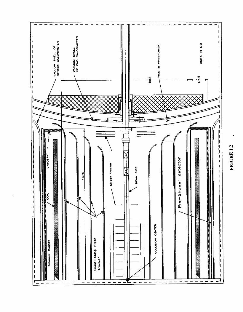
This report details the design of a thin 2 Tesla superconducting solenoid magnet to be installed in the aperture of CC. The arrangement of the new central tracking system including the solenoid magnet is shown in Figure 1.2. Particles outgoing from the interaction point first encounter the thin beryllium beam vacuum tube of the Tevatron, then a set of precision silicon microstrip vertex detectors, a four layer scintillating fiber tracking system, the thin solenoid magnet, and an electron preshower detector. The preshower detector just outside the magnet cryostat will aid in electron identification and will compensate the response of the electromagnetic calorimetry for the effects of unavoidable materials in the solenoid and inner tracking systems.

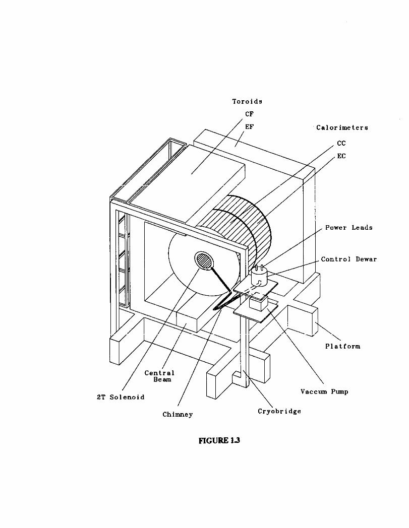
The tracking systems in the bore of the solenoid will be supported by the magnet cryostat vacuum vessel, and the preshower detector just outside the solenoid will likewise be supported by the magnet cryostat, which in turn is supported by the CC vacuum vessel. A perspective view of the solenoid inside the CC (omitting one EC and EF for clarity), together with its chimney and control dewar, is shown in Figure 1.3.

1.3 General Requirements for the Superconducting Solenoid

The overall physical size of the thin 2 Tesla solenoid is determined by the dimensions of the existing aperture of the CC vacuum vessel. The overall dimensions of the proposed solenoid

l-2

are 2.73 meters in length and 1.42 meters in diameter. The central field of 2 Tesla is selected considering the optimization of momentum resolu-

tion Apl/pl and tracking pattern recognition, the overall available space in the CC aperture, and the necessary thickness for the cryostat which depends on considerations of the thickness of the conductor and support cylinder.

Because the mucm toroids are located several meters from the solenoid magnet and sym- metrically placed outside it, there will be modest magnetic interaction between the steel of the mucm system and the solenoid. Much of the magnetic flux generated by the solenoid returns in the space between the cryostat and the muon system. This volume is nearly entirely filled with the uranium argon calorimeters and associated electronics, a scintillator-based intercryostat detector (ICD) system, and the first layer of the muon proportional drift tubes (PDT’s). The Main Ring beam pipe also traverses this space, penetrating the calorimeter vessels themselves.

The effects of this field on the muon PDT’s, where it and the fringe fields from the existing muon toroid coils reaches 500 Gauss have been studied and have been shown to be unimportant. The same is true of the calorimeter. The photomultiplier tubes of the ICD will require replacement or relocation and the Main Ring will require specific attention if it has not been replaced by the Main Injector [5] prior to the installation of the solenoid. The field at the Main Ring beam pipe reaches 300 Gauss and it has been found that a thick iron shielding pipe will be sufficient to protect the Main Ring beam from harmful perturbations due to the solenoid fringe field if the Main Injector is delayed.

The major requirements for the proposed solenoid are as follows:

1. 2 Tesla Central Field: With the present technology and materials for thin coil superconducting solenoids, it is possible to design a solenoidal magnet with a 2 Tesla central field which will operate stably and safely at all times.

2. Uniformity of Magnetic Field: The inside volume of the solenoid which is occupied by the tracking system should have uniform field over as large a percentage of the volume as practical to optimize the pattern recognition and the momentum resolution of charged particles.

3. Geometrical size: The solenoid, together with the preshower detector, must fit in the existing inner clear bore of the DO Central Calorimeter. To make the tracking space as large as possible the cryostat should be made as thin as practical.

4. Thinness in Radiation and Interaction Length: To preserve the present electromagnetic energy resolution of the existing DO calorimeter the materials for the solenoid should be chosen to reduce their radiation and interaction length as much as practical. The effective radiation length of the solenoid

l-3

materials will be utilized as a part of the electron converter, together with a lead sheet wrapped around the outer surface of the cryostat with thickness graded so that the total combined thickness is nearly independent of scattering angle.

5. Chimney: A service chimney carrying cryogen*, magnet high current buses, and vacuum pumpout and relief, must reach the magnet through the narrow space between the CC and EC vacuum vessels. The narrowest space between these calorimeters is 7.6 cm wide, and the chimney must be designed to fit this space.

6. Control Dewar: The control dewar for the solenoid will be mounted on the DO detector cryobridge structure as shown in Figure 1.3. A turbo pump for the magnet vacuum system will also be supported by the cryobridge.

7. Remote Operation: The entire detector system operates in the DO collision hall which is a radiation environment when the Tevatron and Main Ring are operating. There is no personnel access to this hall at this time. The magnet system must permit full remote operation, including cool down, energization, de-energization for field reversal, quench recovery, and warmup, without operator access to the magnet cryostat, service chimney or control dewar.

The major parameters of the DO Solenoid design are shown in Table 1.1. The parameters of the proposed solenoid are compared with those of the ZEUS [7] detector solenoid at DESY and the CDF(8] solenoid at the Tevatron in Table 1.2. The ZEUS solenoid was designed with a central field of 1.8 Tesla with similar field homogeneity requirements, but placed asymmetrically relative to the steel structure of the ZEUS detector. The stored energy of the proposed DO solenoid is approximately 5.6 MJ. This stored energy is much smaller than the 30 MJ of CDF or the 12.8 MJ of ZEUS, and the stored energy per unit cold mass of the DO coil has been made lower than either of these magnets as well. Because design choices for the DO solenoid can be made which are fundamentally conservative, the proposed solenoid while technically advanced does not surpass state-of-the art and will lend itself to ready fabrication.

l-4

References

[1] Design Report, “The DO Experiment at the Fermilab Antiproton-Proton Collider”, November, 1984.

[2] S. Abachi, et.& “The DO Detector”, Nuclear Instruments and Methods in Physics Research, A338, 185, 1994.

[3] S. Abachi, et.aL, “Beam Tests of the D0 Uranium Liquid Argon End Calorimeters”, Ndclear Instruments and Methods in Physics Research, A324, 53, 1993.

[4] C. Brown,el.al, “D0 Muon System with Proportional Drift Tube Chambers”, Nuclear Instruments and Methods in Physics Research, A279, 331, 1989.

[5] G. Dugan, Accelerator Upgrade and the Main Injector, DO Note 976, June 12, 1990.

[6) DO Upgrade, D0 UPG-01, 10/18/1990; also P823, (DO Upgrade), DO Note 1148, June 18, 1991; also E823, (DO Upgrade), DO Note 1426, May 20, 1992.

[7] A. B. Olivia, &al., “ZEUS Magnets Construction Status Report”, Proceedings of the ll’* International Conference on Magnet Technology, 229, 1989.

[B] R. W. Fast, &al., “Testing of the Superconducting Solenoid for the Fermilab Collider Detector”, Advances in Cryogenic Engineering V31, 181, 1986, Plenum, NY.

l-5

TABLE 1.1: DO Solenoid Parameter Summary Parameter Selected Value

I

Central Field 2T Operating Current 4825 A Charging Time 7min Stored Energy 5.6 MJ Inductance 0.48 H Protection Resistor 0.048 Ohm Cryostat Dimensions:

Length 273 cm OD 141.6 cm ID 106.6 cm

Material: Coil Support Cylinder Aluminum 5083-O Cryostat Aluminum 5083-O

Vacuum Vessel Design Designed for full vacuum and

Control Dewar Design Cold Mass Supports:

Shipping

At 4.7 K

Superconductor:

Conductor Grade I Conductor Grade II

6.4 psi internal pressure Designed to ASME code

Designed for 4g radial Designed for 6g axial with shipping restraints

High-purity aluminum stabilized multi- filamentary Cu-NbTi Rutherford cable 5.125 x 15 mm 3.820 x 15 mm

Cryogenics: Temperature of Cold Mass

maximum nominal

Coil Cooling Technique Radiation Shield Cooling Refrigeration System

4.9 K 4.7 K Indirect, with 2 phase LHe forced flow LN2 forced flow Shared Fermilab 600 W Satellite Refrigerator

l-6

TABLE 1.2: COI mparison Parameter units

( zentrai Field ‘ stored Energy 1 Radiation Thickness 1 [nductance Total Weight ( zold Mass I Cryostat Outside Radius I Cryostat Inside Radius I Cryostat Length I Coil Winding:

Support Cylinder Thickness No. of Layers Inner Radius Length No. of Turns

T MJ A H kG kG cm cm cm

mm mm cm em

Total Amp-Turns Conductor:

10s I

Conductor Grade I Conductor Grade II Conductor Radial Width Turn to Turn Ins Al:Cu:NbTi I Al:Cu:NbTi II Stabilizer Al

Superconductor: Form Dimensions Operating Current Short Sample Current

@ (4c.h w Z,/I, (load line)

of Thin Solenoids

7

2.0 5.6 0.87 0.48 2300 1460 70.7 53.3 273

1.8 12.5 0.9 1.28

2000 111 86 285

15 18 16 2 2 1 58.7 92.5 148.3 256.6 248.7 479.4 1010 907 1150 4.87 4.54 5.75

mmxmm 3.820 x 15 4.3 x 15 mmxmm 5.125 x 15 5.56 x 15 mm 15 15 mm 0.5 0.5 parts 19.3:1.3:1 lE:l.l:l parts 13.8:1.3:1 14:1.1:1 Purity 99.996 99.996

mm2 A

tiK) %

Cable Cable Monolith 8.20 eff 8.4 eff 6.93 4825 5000 5000 14400 15000 10400 (2.3, 4.7) (2.3, 4.5) (1.5, 4.4) 55 54 60

CDF

1.5 30 0.83 2.4 11100 5570 167.7 142.9 507

3.89 x 20 -

20 0.1 21:l:l -

99.99

l-7

I

TABLE 1.2 (cant): Camp Parameter

------I

Details of Cryostat: Total Radial Thickness Vacuum Shell Aluminum Outer Vacuum Shell Thickness Cuter Radiation Shield Thickness LHe Cooling Pipe Conductor+InsuIation Inner Radiation Shield Thickness Inner Vacuum Shell Thickness AsiaI distance between Crvostat & Coil Bulkhead Thickness

Decentering Force: AXidal Radial

Df Thin Solenoids larison 4 units CDF

mm

mm mm mm ID IIlIIl mm mm

174.5 5083-O 8 1.6 15 35.4 1.6 6.4

250 6063-T6 12 3.0 18 32 3.0 5.0

248 5083-O 19 2.0 16 23.5 2.0 6.4

mm 53.0 182 137 mm 20 30 25.4

104N/m 6.9 ( 5 Tons) 1760 104N/m 1.1 2 1230

l-8

MUON MUON Toroid PDT Chambers EF

MUON Toroid CF

(to be replaced) cc EC’S

L&id Ar Calorim&zrs

D@ Detector

Figure 1.1

:

5 ;:, a?

20 >w 3tl

\

!

L

-

-

-

-

-

-

F

8 /

-

- - - -

-I I

/ -

.-

Toroids

CF

2T

& /,r”rs

, Power Leads

Control Dewar

\ Platform

\ Vaccum Pump

Chimney Crybbr idge

FIGURE 13

CHAPTER 2

COIL DESIGN

2.1 General Features

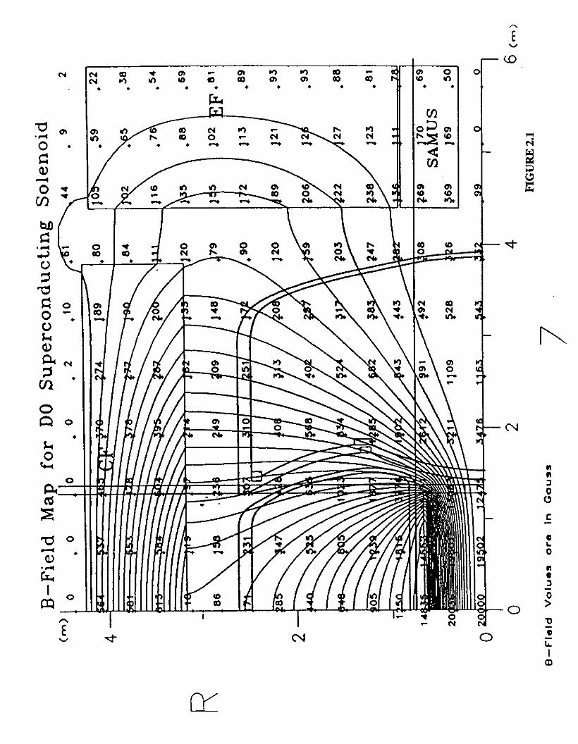
A cross section of the DO detector together with the solenoid is shown in Figure 2.1 with flux lines and field values superimposed on it from a 2D calculation of the solenoidal field. From the values of the field shown in Figure 2.1 it is seen that the field of the solenoid rapidly falls beyond the end of the magnet. In order to maximize the field uniformity inside the bore of the solenoid over as large a volume as practical the current density in the windings is made larger at the ends of the coil. This leads to the use of two grades of conductors with different thicknesses. Both grades of conductors are made with a superconducting Rutherford cable of multiiilamentary Cu-NbTi strands stabilized with pure aluminum. For specificity, the basic strand chosen is of the WC-type with Cu:NbTi ratio 1.3:1 and diameter 0.808 mm.

The solenoid is wound with two layers of aluminum stabilized superconductor to achieve the required linear current density for a 2 Tesla central field, as shown schematically in Figure 2.2. The support cylinder is located on the outside of the winding to support the radial Lorentz forces on the conductor.

The use of pure aluminum in the conductor yields a low resistivity stabilizer for the superconductor while reducing the interactions of particles in the material of the conductor. Aluminum is chosen for the support cylinder and vacuum vessel of the magnet cryostat also to achieve low particle interaction rates in the balance of the magnet structure.

The coil is indirectly cooled by two-phase liquid helium flowing through an aluminum cooling tube which is welded to the outside surface of the support cylinder. For stability the coil relies on the specific heat and high thermal conductivity of the high purity aluminum stabilizer and by a conservative margin of the critical current of the superconductor beyond the operating current of the magnet. The presence of the support cylinder ensures quench safety by the rapid spreading of the normal zone in the event of a quench (the “quench-back” effect) [l], a typical feature of magnets of this type.

2.2 Conductor Selection

For practical reasons the maximum operating current of the magnet is set at 5000 A and the size of the conductor and the superconducting insert is chosen accordingly. Considerations of available technology for the coextrusion of pure aluminum and the margins of stability desired for such a magnet led to a choice of overall conductor cross-section and a two-layer winding design. By adjusting the conductor final size accordingly two grades of conductors

2-l

are specified so that increased current density can be provided at the ends of the coil to improve the field homogeneity.

The cross sections of the two grades of aluminum stabilized conductor are shown in Figure 2.3. Both grades use the same superconducting insert and only the amount of aluminum stabilizer is varied between them. The larger conductor is 5.125 mm wide and the smaller conductor is 3.820 mm wide. Both conductors have a radial height of 15 mm for simplicity of forming joints between the two grades and overall ease of winding. The cable within the conductor is placed at a location in the cross-section that is most appropriate for the coextrusion process and the subsequent bending of the finished conductor as the coil is wound. The superconductor is shown placed nearest the inside radius of the conductor in Figure 2.3. This choice of location maximizes the region of pure aluminum that can be used for the making of welded joints between conductor lengths during coil winding. The finished overall dimensions of the conductor are readily held to tight tolerances to ensure uniform coil winding. The final shape of the conductor may be keystoned slightly if necessary to accommodate any distortion due to the rather high prestrain caused by conductor winding.

There are several considerations to be addressed when making a choice between monolithic and cabled superconductors. Earlier thin solenoids such as CDF [2] were made with monolithic superconductors. More recent solenoids (ALEPH [3], ZEUS [4], CLEO II [5], and the SDC model [S]) were made with cabled superconductors. A cabled superconductor is preferred for the following reasons:

1. Longer lengths of finished conductor are more easily made. With a cabled superconductor, original billet size does not limit the length of finished conductor that can be made. Occasional strand joints are permissible and the overall risk of the conductor production is lessened.

2. The technique of coextruding high purity aluminum with a cabled superconductor is well established in industry. Adequate capability has been demonstrated for producing finished conductor of the required length having high quality intermetallic bonding, while preserving excellent low resistivity in the aluminum and maintaining tight control over finished conductor shape tolerances.

3. Many industrial suppliers have produced high quality stranded cabled conductor for recent accelerator projects including HERA, RHIC, and the SSC, as well as for other commercial applications. Thus suitable cabled conductor is readily available and may cost less than a custom made monolithic conductor. Because the cable strand design is not greatly restricted by the final design of the finished conductor the delivery time of the finished conductor can be lessened as well.

4. With a bending radius of about 0.58 meters as required by the size of the solenoid, a superconducting cable insert should permit adequate formability of the conductor

2-2

during coil winding. The location of the cable within the finished conductor cross section must be chosen with this coil winding requirement in mind.

The desired superconductor critical performance is shown in Figure 2.4. The load line of the magnet and the operating line for the peak field on the conductor is shown. The peak field on the conductor is 2.2 T when the magnet central field is 2.0 T, as shown in Figure 2.4. The peak field occurs in the inner layer winding at the point where the current density increases near the end of the coil. The critical curves for the superconductor are generated by scaling,from SSC-type cable performance. At 2 Tesla, the typical current carrying capacity of the SSC 30 strand cable is 34500 A at 4.2 K [i’]. This leads to 18400 A for the 16 strand cable at 4.2 K. At an operating temperature of 5.1 K, this cable would have a critical current of about 14460 amperes; the magnet operates at 55% of this current (along the load line) at design field.

2.3 Winding Design

The two grades of conductor are used in both layers. The middle section of each layer is wound with the wider conductor and the end sections with the narrower conductor. The transition point between the two grades of conductor in the inner layer occurs at z= zt 0.953 meters from the center, while for the outer layer this transition occurs at a= It 0.653 meters from the center. With this straight-forward grading of the current density it is possible to achieve a sufficiently uniform field inside the solenoid volume as will be described in Chapter 3. In order to reduce the maximum field on the conductor the outer layer transition point occurs at a smaller z than the transition in the inner layer. A summary of the calculational parameters of the solenoid is shown in Table 2.1. Note the current blocks correspond to the radial locations of the superconducting inserts in the conductors, with the current smeared uniformly in a. The field calculations resulting from this winding design are described in Chapter 3.

2.4 Conductor Joints

There are four places in the solenoid where the conductor width changes, two on the outer layer and two on the inner layer. At these locations the two grades of conductors are joined with a lap joint and edge-welded as indicated in Figure 2.2. The welding of a 40 cm length is done at four places along the one overlapping turn of both grades of conductors. This will make an estimated resistivity of 4 x 10-i’ Ohm at 4.2 K at each joint [2]. This type of joint entails the effective loss of one turn per transition point. This loss has been incorporated in the field calculations described in Chapter 3. It is desireable that there be no other joints in the coil.

2-3

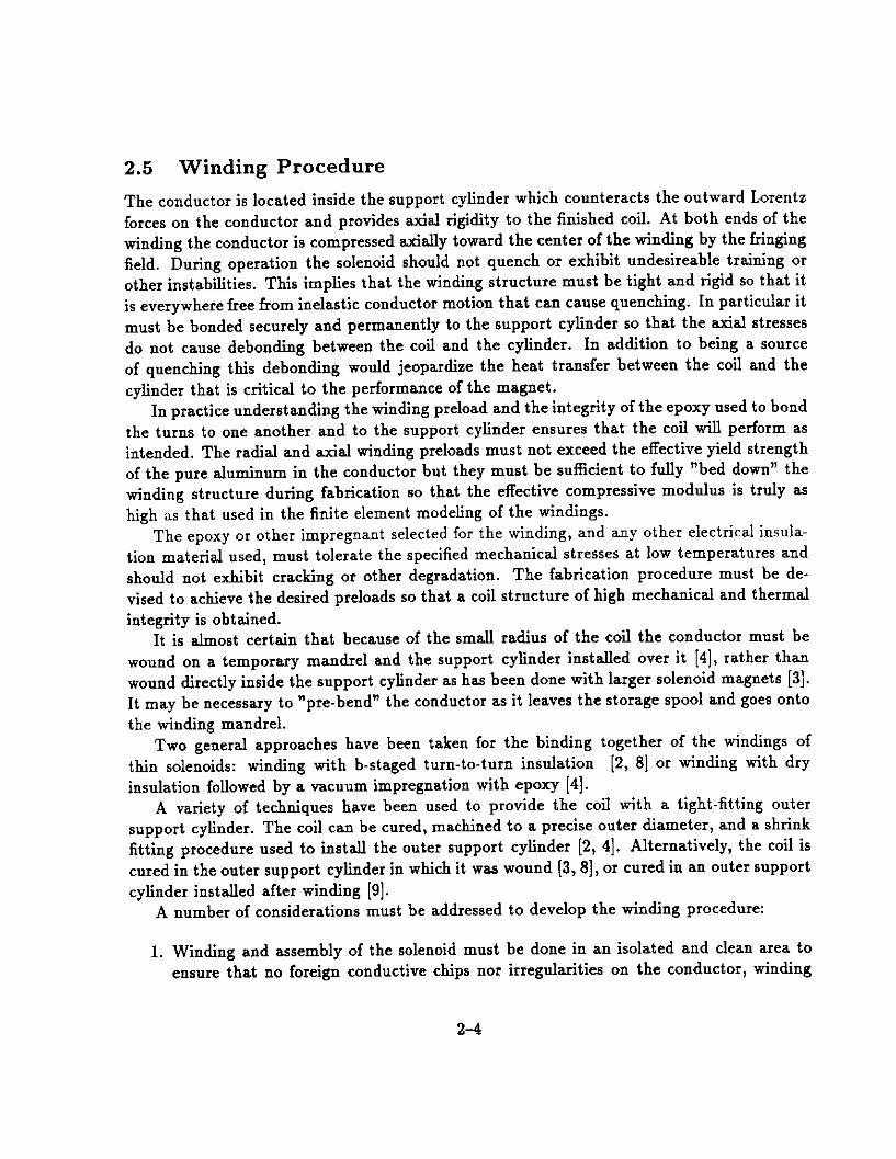
2.5 Winding Procedure

The conductor is located inside the support cylinder which counteracts the outward Lorentz forces on the conductor and provides axial rigidity to the finished coil. At both ends of the winding the conductor is compressed axially toward the center of the winding by the fringing field. During operation the solenoid should not quench or exhibit undesireable training or other instabilities. This implies that the winding structure must be tight and rigid so that it is everywhere free from inelastic conductor motion that can cause quenching. In particular it must be bonded securely and permanently to the support cylinder so that the axial stresses do not cause debonding between the coil and the cylinder. In addition to being a source of quenching this debonding would jeopardize the heat transfer between the coil and the cylinder that is critical to the performance of the magnet.

In practice understanding the winding preload and the integrity of the epoxy used to bond the turns to one another and to the support cylinder ensures that the coil will perform as intended. The radial and axial winding preloads must not exceed the effective yield strength of the pure aluminum in the conductor but they must be sufficient to fully “bed down” the winding structure during fabrication so that the effective compressive modulus is truly as high irs that used in the finite element modeling of the windings.

The epoxy or other impregnant selected for the winding, and any other electrical insulation material used, must tolerate the specified mechanical stresses at low temperatures and should not exhibit cracking or other degradation. The fabrication procedure must be de- vised to achieve the desired preloads so that a coil structure of high mechanical and thermal integrity is obtained.

It is almost certain that because of the small radius of the coil the conductor must be wound on a temporary mandrel and the support cylinder installed over it [4], rather than wound directly inside the support cylinder as has been done with larger solenoid magnets [3]. It may be necessary to “pre-bend” the conductor as it leaves the storage spool and goes onto the winding mandrel.

Two general approaches have been taken for the binding together of the windings of thin solenoids: winding with b-staged turn-to-turn insulation [2, 81 or winding with dry insulation followed by a vacuum impregnation with epoxy [4].

A variety of techniques have been used to provide the coil with a tight-fitting outer support cylinder. The coil can be cured, machined to a precise outer diameter, and a shrink fitting procedure used to install the outer support cylinder [2, 41. Alternatively, the coil is cured in the outer support cylinder in which it was wound (3,8], or cured in an outer support cylinder installed after winding [9].

A number of considerations must be addressed to develop the winding procedure:

1. Winding and assembly of the solenoid must be done in an isolated and clean area to ensure that no foreign conductive chips nor irregularities on the conductor, winding

2-4

mandrel, or support cylinder surfaces remain to jeopardize the electrical integrity of the coil.

2. If winding on the inside of the support cylinder is not feasible, a temporary collapsible but rigid winding mandrel can be made which has an accurate and smooth outer diameter machined to a tolerance of at least f 0.05 mm.

3. A layer of fiberglass-epoxy insulation several millimeters thick is built up on the mandrel, using b-staged sheets or the like, compressed to high glass fraction and cured as specified. Considerations of debonding the mandrel from this layer after the coil is finished must be addressed when this insulation layer is designed.

4. The insulated surface of the mandrel is then machined to an accurate and smooth diameter to a tolerance of at least + 0.05 mm. The final thickness of the insulation is arbitrary, but it needn’t exceed a millimeter or so. The final dimeter of the insulated mandrel is chosen to be that required by the coil design.

5. End flanges to support coil winding and axial preloading are then attached to the winding mandrel. Depending on subsequent fabrication steps, these flanges may require later replacement. The final shape and geometry of the winding surface is documented by careful measurement.

6. After providing for the doubling of the input bus to the magnet coil, winding then proceeds. The input bus can be made of two standard conductors edge-welded for 10 cm. long every 30 cm. The details of conductor final inspection and insulation, winding pretension, temporary axial clamping, etc., take place as required by the final winding design choices. Provisions for making joints between conductor grades is made when transitions between current densities is required, as is constant monitoring for shorts to ground and turn-to-turn, as well as documenting the geometry of the windings and joint locations as the layer proceeds. When the first layer is completed, the winding transition to the second layer is provided.

7. Layer-to-layer insulation is installed, and if a b-staged (or wet layup) winding design is used, it may be necessary to clamp and cure the first layer at this time. The second layer is wound much like the first, with the same attention to winding detail as outlined in step 6 above.

8. When the final turns are installed, the outlet bus is reinforced like the inlet bus as described in step 6. As with the inlet bus, extra length is left attached and appropri- ately stored so that the magnet buswork in the service chimney can be later installed without unnecessary joints.

2-5

9. When the second layer is completed, ground plane insulation is added. If a b-staged winding design was used this might be more b-stage sheets overwrapped and the coil clamped and cured. If an impregnated winding design is chosen this might be bare glass cloth, after which the coil is clamped, enclosed, and then vacuum impregnated and cured. The outer surface of the coil is machined to a precision of at least * 0.05 mm, leaving a total outer insulation thickness of about 2 mm. The final diameter is accurately measured and the coil is tested for shorts to ground.

10. The outer support cylinder is machined to an interference ID to the coil. Before final machining the helium cooling tubes and support attachments can be welded onto the OD of the support cylinder.

11. The machined support cylinder is heated to a temperature rise of 100 Celsius. The cylinder will expand approximately 3.1 mm on the diameter so that the final room temperature interference can be chosen with regard to the clearance needed for the heated insertion procedure. The cylinder is then lowered over the coil which is standing vertically on its axis, and allowed to cool. The coil may be lubricated with a suitable epoxy prior to installation of the support cylinder.

12. Depending on the winding design details the end flanges of the support cylinder are attached to it and preloaded if necessary unless they are already in place. The collapsible winding mandrel is removed and final measurements and tests are then made on the completed winding.

13. The coil temperature sensors and potential taps are installed and the current buses routed and clamped as necessary.

References

[l] M. A. Green, “Large Superconducting Detector Magnets with Ultra Thin Coils for use in High Energy Accelerators and Storage Rings”, LBL - 6717, Aug. 1977, and Proceedings of the 6’h International Conference on Magnet Technology, Bratislava, 1977.

[2] R. W. Fast, et al, “Design Report for an Indirectly Cooled 3-m Diameter Supercon- ducting Solenoid for the Fermilab Collider Detector Facility”, Fermilab internal report TM-1135, Oct. 1, 1982.

[3] J. M. Base, et al, “Design, Construction and Test of the Large Superconducting Solenoid Aleph”, IEEE Transactions on Magnetics, Vol 24, No. 2, March 1988.

[4] A. Bonito-Oliva, et al., “Zeus Magnets Construction Status Report”, Proceedings of the llo’ International Conference on Magnet Technology, p 229, Tsukuba, Japan, 1989; and

2-6

A. Bonito-Oliva, &al, “Zeus Thin Solenoid: Test Results Analysis”, IEEE Transactions on Magnetics , Vol 27, No. 2, March 1991.

[5] D. M. Coffman, et al., “The Cleo II Detector Magnet: Design, Tests, and Performance”, IEEE Transactions on Nuclear Science, Vol 37, No.3, 1990.

[6] A. Yamamoto, et al., “Design Study of a Thin Superconducting Solenoid Magnet for the SDC Detector”, Proceedings of the Applied Superconductivity Conference, Chicago, 1992.

[7] D. Christopherson, et al., “Summary of the Performance of Superconducting Cable Pro- duced for the Accelerator System String Test Program”, Supercollider 4; Proceedings of the Fourth IISSC, p.25, 1992

[8] R. Q. Apsey, et al., “Design of a 5.5 Metre Diameter Superconducting Solenoid of the DELPHI Particle Physics Experiment at LEP”, IEEE Transactions on Magnetics, Vol MAG-21, No. 2, 1985.

[9] M. Wake, et al., “A Large Superconducting Thin Solenoid Magnet for Tristan Experiment VENUS at KEK’, IEEE Transactions on Magnetic+ Vol MAG-21, No. 2, 1985.

2-7

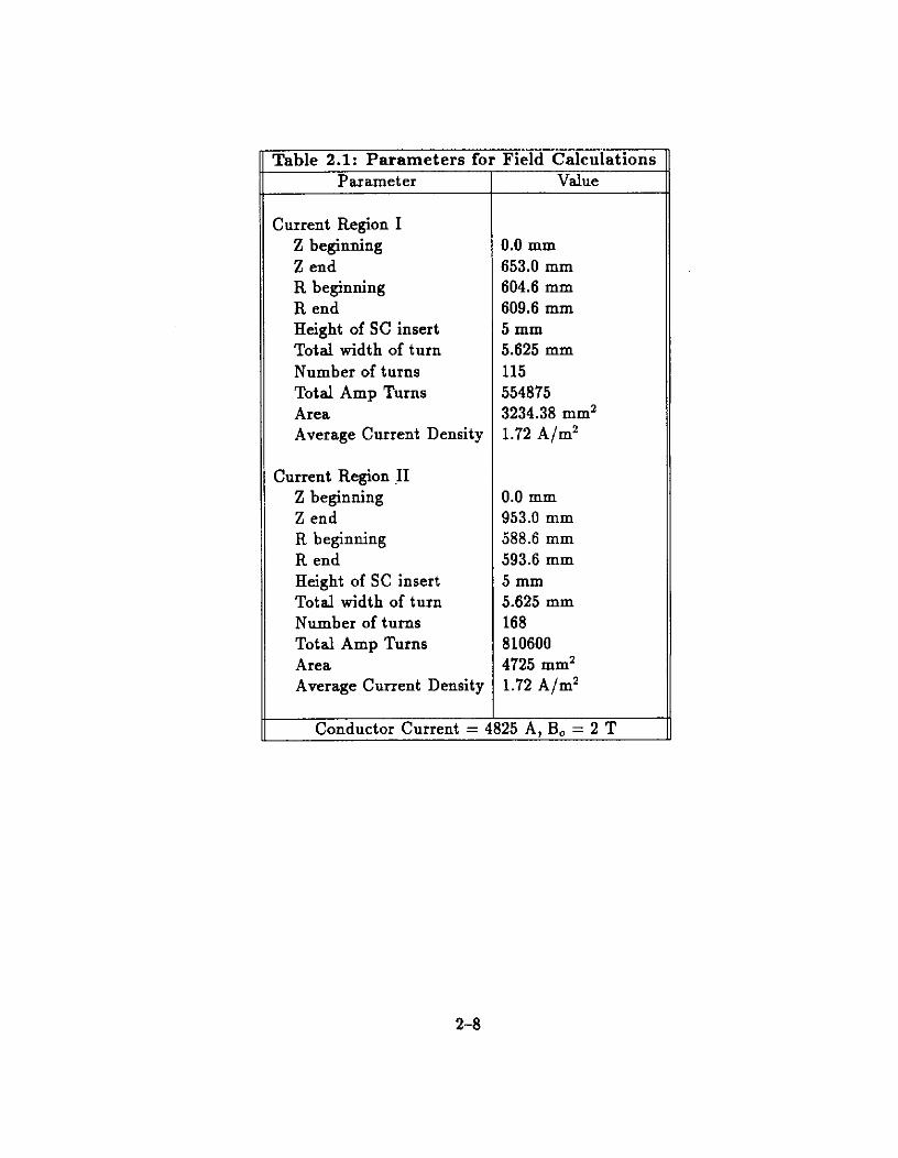
Table 2.1: Parameters for Field Calculations Parameter Value

Current Region I Z beginning Z end R beginning R end Height of SC insert Total width of turn Number of turns Total Amp Turns Area Average Current Density

0.0 mm 653.0 mm 604.6 mm 609.6 mm 5mm 5.625 mm 115 554875 3234.38 mm’ 1.72 A/m2

Current Region II Z beginning Z end R beginning R end Height of SC insert Total width of turn Number of turns Total Amp Turns Area Average Current Density

0.0 mm 953.0 mm 588.6 mm 593.6 mm 5mm 5.625 mm 168 810600 4725 mm’ 1.72 A/m2

Conductor Current = 25 A, B, = 2 T

2-8

Table 2.1: Parameters for Field Calculations Parameter I Value

I Current Region III Z beginning Z end R beginning R end Height of SC insert Total width of turn Number of turns Total Amp Turns Area Average Current Density

653.0 mm 1282.5 mm 604.6 mm 609.6 mm 5mm 4.32 mm 146 704450 3153.6 mm* 2.23 A/m’

Current Region IV Z beginning Z end R beginning R end Height of SC insert Total width of turn Number of turns Total Amp Turns Area Average Current Density

953.0 mm 1282.5 mm 588.6 mm 593.6 mm 5mm 4.32 mm 76 366700 1641.6 mm’ 2.23 A/m2

Conductor Current = 1 125 A, B, = 2 T

2-9

0 00

.

2 0 -

!2-

E

t 0 : 3 >o u % i2 I m

Lm :

EE EEEE EEEEEE

-Ii c -

SL. c 071 .- N 0 ‘,; 00; bt, 1 v. m-i InQY

; 3 .

X

u f *f * co’0

XE u 0)

:.E ; Qy1 a-

IEm o”

b

u) L? -GO

II ” ;r .f jj 1 3

e ri

N In -i -i II II

7;

2

A -*

t;

in

r

g /

l-

CHAPTER 3

FIELD AND FORCE CALCULATIONS

3.1 2-Dimensional Field Calculations

Because the overall geometry of the solenoid inserted in the existing toroid magnet system of the D0 detector is rather complicated, field calculations were done in three steps. The first step was to model the solenoid surrounded by the thick steel of the toroidal magnet system but with the latter unexcited. This calculation provides a field map sufficiently accurate to enable the evaluation of potential interaction between the solenoid and the various existing detector elements in the fringe field of the solenoid.

In this first calculation the system was assumed axisymmetric and field values were calculated with the 2 dimensional finite element analysis program ANSYS [l]. The result is shown in Figure 2.1. In this calculation, the solenoid is excited, but not the toroids. The magnetic field of the solenoid on the surface of the toroidal steel is up to 330 Gauss.

To model the solenoidal field more accurately near and inside the coil a much more detailed local calculation was required. Using the solution from step one, boundary. conditions for a smaller region containing the coil were obtained and a second calculation on a much finer mesh (2 cm) was made of the region near the solenoid coil. The restricted boundary was remote enough from the solenoid so as not to significantly affect the calculation but the boundary conditions were necessary to constrain the new solution. The field values from this solution are particularly valuable for studying the homogeneity of the field in the bore of the magnet, especially as it relates to tracking issues such as pattern recognition and charged particle momentum resolution API/PI.

In a final step, a very fine mesh (5 mm) was used for a solution of the field near the coil. This solution was useful in studying the field in regions within the coils.

3.2 Detailed Field Calculations Near the Solenoid

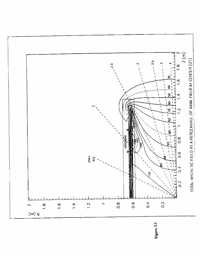
The total magnetic field distribution and axial magnetic field distribution inside the solenoidal volume are shown in Figures 3.1 and 3.2, respectively. The field values in these figures are normalized to the central field value of the solenoid (2 Tesla), and plotted as a percentage of this value. The two field peaks near the end of the winding are due to the increased current density caused by the change of conductor width. The locations where the change of conductor widths and missing turns occur are marked with arrows. A detailed study shows that the maximum total magnetic field is 2.174 T at the outside edge of the inner layer

3-l

conductor. Select values of the pseudorapidity variable q = -log(tan0/2) which is derived from the scattering angle 0 are also plotted in these figures.

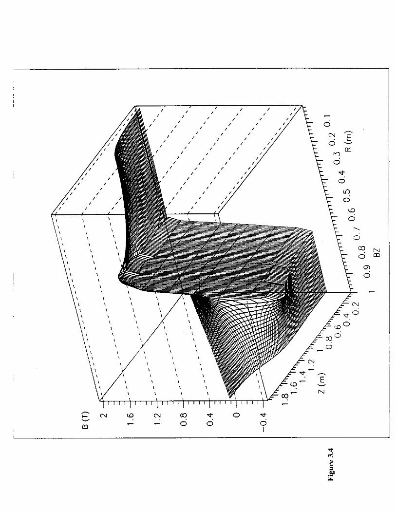
A 3dimensionai isometric representation of the axial field distribution inside the solenoidal region is shown in Figure 3.3. From this figure it is clearly seen that the axial field is rea- sonably constant over the majority of the solenoidal volume. Figure 3.4 shows the reverse side of this plot illustrating the negative return tlux distribution.

3.3 Integrated Field Uniformity

To quantitatively describe the inhomogeneity of the magnetic field inside the solenoidal volume, a calculation that defines the inhomogeneity of the field as a function of scattering angle from the center of the magnet is made. This calculation takes the form of an integral over the path along an angle from the center to the coil or the coil end plane, depending on the azimuthal scattering angle 0:

Inhomogeneity = - ‘(J3z - BJdl

where I?, is the axial magnetic field along the path L(B), p the endpoint of the path, 0 the scattering angle, and B. the field at the center of the solenoid ( 2 Tesla).

The result of this calculation as a function of the angle B is shown in Figure 3.5. The integrated field error is less than 3% in the range from 28 degrees to 152 degrees in scattering angle. There are slight fluctuations caused by the missing turns where the conductor transition joints are located, but these are unimportant.

3.4 3-Dimensional Field Calculations

A three dimensional field calculation of the entire detector was performed by the TOSCA [2] program using a 10 cm grid. First the field of the existing toroid system was calculated without the the solenoid in order to compare the results to the measured values from the toroids. When the B-H curves used with the TOSCA program were modified to give consistent data with the measured results, the solenoidal coils were added and the results were compared to the two dimensional ANSYS calculation. The flux distribution in the toroid steel is not deeted greatly by the fringing field of the solenoid, partly because the toroid steel is already strongly saturated by the toroid coils. There is however a small effect noticeable along the toroid steel surface caused by the solenoid.

3-2

3.5 Decentering Forces

Three approaches have been taken to estimate the forces between the coil and the toroid steel; one is totally analytic, one is mixed (i.e. partly analytic and partly discrete) and the third uses ANSYS to estimate the axial forces. Because the coil is nominally centered in the yokes of the EF and CF toroids the net force on the coil is nominally zero; the calculations in all cases predict that the radial and the axial forces generated by small displacements are decentering. Because the coil is quite far from the steel both radially and axially the forces for reasonable displacements are predicted to be modest. The corresponding minimum stiffness required of the cold-mass suspension system is likewise modest.

3.5.1 Analytic Approach: “Ideal Dipole”

For the fully analytic approach the solenoid is modeled as an ideal dipole and the toroid yokes as semi-infinite sheets of infinitely permeable iron. The dipole moment of the ideal dipole is just the total solenoidal current times the cross-sectional area of the coil, and the forces are generated by this dipole interacting with image dipoles mirrored in the iron.

The net axial force on an ideal dipole centered between semi-infinite regions of infinitely permeable steel separated from one another a distance 2D is of course zero, but if the dipole is shifted an amount A off center axially it can be shown that a decentering force created by the image dipoles in the EF steel acts on the dipole:

F ~.,3Ms ii ozid

= S’

Hence, for the solenoid in the EF steel, the axial decentering force,‘in the direction of A is:

F

a

= (47r x 1V7) x 3 x (6.08 x lOs)* N

.*id 4rr x (4.45) [;I

= 6.72 x lo3 [El,

inserting the values pertaining to the DO solenoid. The cold-mass suspension system must have axial stiffness greater than this to support the coil stably. For an axial displacement of e.g. 2.5 cm, the decentering force in the direction of the displacement is F = 6.72 x lo3 x 0.025 N = 168 N.

For the solenoid in the CF steel, it can be shown that the radial decentering force due to image dipoles mirrored in the steel, in the direction of the displacement A, is:

F p0M2 ii radial = D’

3-3

Again inserting the values pertaining to the D0 solenoid,

F

Ti rodid

= 1.10 x 10’ $1.

For a radial displacement of e.g. 2.5 cm the decentering force in the direction of the displacement is F = 1.10 x lo4 x 0.025 N = 278 N.

3.5.2 Mixed Approach: “Image Solenoid”

For the “image solenoid” analytic approach the primary solenoid is subdivided into many current loops with each loop subdivided into many small phi-segmented current elements, and the forces generated by solenoids mirrored in the CF and EF steel yokes. The fields of the image solenoids are calculated by subdividing them in the same fashion as is done for the primary solenoid, and using a subroutine which evaluates elliptical integrals to provide the fields at each segment of current of the subdivided p coil. The solenoids are subdivided into 20 axial and 10 radial current loops, and each loop divided into 40 phi-segments. This level of discretization is sufficiently accurate to predict the central fields to l/4 %.

The image field $(r, z) at a current element at (r,a) of the primary solenoid is a sum of

J!? + L!?, where, explicitly, @(T,z) = B(r,z-2(D-A)), and @‘(r, z) = B(r,z+2(D + A)). The force on the current element is just the vector product of this field and the current in the element times its length; the total force on the solenoid is then a sum over all the current elements in the coil.

When the parameter A was set to zero the net calculated forces in the transverse and axial directions were less than 10-*N, indicating that the discretizations were adequate.

For A = 10 cm. we obtain

F* e Fv x 0.0 N

F, = +0.625r103 N.

Assuming linearity for small displacements A, the axial decentering force in the direction of A is predicted to be:

F

a orid = 6.25 x 103$.

For an axial displacement of e.g. 2.5 cm, in the direction of the displacement, F = 6.25 x 10s x 0.025 N = 156 N.

For the radial case, the solenoid is located between two semi-infinite sheets of steel above and below it, and the forces on the solenoid are calculated as described above. The results

for A = 10 cm. are:

FZ z F, x 0.0 N

Fv = $0.801 x lo3 N.

Again assuming linearity for small displacements,

F

a radio1 = 8.01 x lo+],

in the direction of A. For a radial displacement of e.g. 2.5 cm, in the direction of the displacement, F = 8.01 x IO3 x 0.025 N = 200 N.

These results are quite comparable to those obtained from the “ideal dipole” approach, although since the ideal solenoid approach calculates the image fields directly without using any “dipole approximations”, it might be expected to give a more realistic result.

3.5.3 filly Discrete Approach: ANSYS

The axial decentering force has also been calculated using ANSYS by making a 2-dimensional axisymmetric model of the entire solenoid and toroid systems. In this model the solenoid itself is shifted by 2.5 cm on the z axis and the resultant force computed by summing all the axial forces on the solenoid. The total axial decentering force is 1731 N (0.176 metric tons, or 389 lb) corresponding to 6.9 x lo4 N/m.

The estimated forces for the solenoid are in general much smaller than those for magnets which involve steel in the near vicinity, e.g. ZEUS, where the solenoid is placed asymmetrically and the axial decentering force is 5 Tons, or for CDF where the axial decentering force is 1.8 Tons/cm.

3.6 Stress Calculations by ANSYS

Because the toroid steel is remote from the solenoid there is a substantial radial field component along the coil which increases toward the ends of the magnet. This radial field produces significant s&l compressive force in the coil which increases with increasing distance from the coil center. ANSYS was used to calculate the corresponding stress and that from the hoop loads as well.

Provided with the appropriate geometry in a predefined region ANSYS first calculates the magnetic field, and then the Lorentz forces on the coil, for the problem specified. Then ANSYS evaluates the stresses on the coil and support cylinder elements specified in the region. For these stress calculations the outer air boundary was constrained to a iixed potential determined from a full scale 2-dimensional axisymmetric model of the detector including the toroid magnets. The mesh for the coil and support cylinder in this full scale

3-5

model were not fine enough to determine peak stresses on the coil. Therefore a much finer mesh and model were created around the solenoid for stress analysis and the results of this smaller model are used in this analysis.

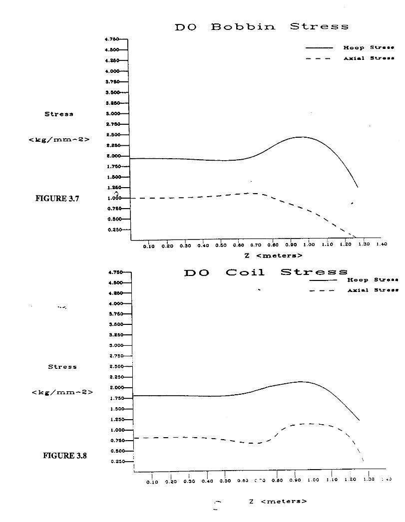
A number of assumptions about the solenoid model are implicit in this analysis. The model is 2-dimensional and is assumed to be axisymmetric, and the middle point of the solenoid and support cylinder (the left boundary of the model) is constrained to a movement of 0.0 m in the Z direction. The bond between the coil and support cylinder is assumed inseparable, and the modulus of elasticity used for the solenoid is 6.86 x 10”N/m2 for the combined structure of the coil and support cylinder. This value comes from the CDF R&D test coil (31. The results of the ANSYS calculations are shown in Figure 3.7 and 3.8 and the extrema of these curves are tabulated in Table 3.1. Note that although the origin of the loads on the coil are the conductors themselves, the model incorporates the support cylinder together with the coil as a monolithic structure.

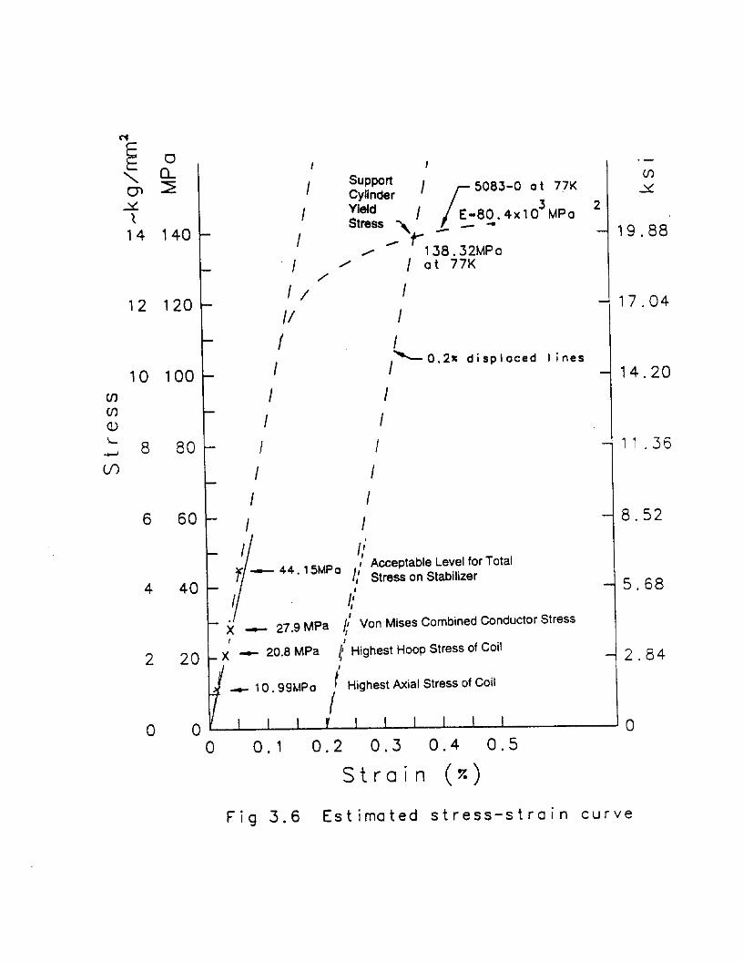
The hoop stresses generated in the coil are equilibrated by strain in the support cylinder and coil, the highest hoop stress in the conductor is 20.8 MPa (Table 3.1). From Figure 3.8 it is seen that the peak axial and hoop stresses in the coil are at nearly the same Z location. Thus we combine them using the Von Mises criterion (they are the principle stresses) to obtain an effective total stress of 27.9 MPa. This is well within the limit set for the pure aluminum, taken to be 44.15 MPa (6400 psi), as shown in Figure 3.6.

3.7 Analytic Hoop Stress Analysis

When cooled to 5.0 K, the length of the outer support cylinder is reduced by AL = L x 4.3 x 10e3 = 11 mm due to thermal contraction effects. Because the cylinder is axially constrained only at the current lead end (see Chapter 4), most of this motion appears at the other end of the coil and no new stresses on the coil result. Similarly, the radius of the support cylinder is reduced by AR = R x 4.3 x lo- s = 2.8 mm during cooldown, and the radial support system is designed so that small added stresses on the coil result from this motion.

During cooldown the support cylinder is cooler than the conductor and this will ensure that the support cylinder always remains compressively loaded onto the coil windings. Be- cause the temperatures experienced in the support cylinder and the coil always remain well below 1OOK during a quench the support cylinder will not be subject to unwanted differential thermal expansion from the coil. Warm up of the magnet will be achieved without generating excessive temperature difference between the coil and the support cylinder.

When the magnet is excited, the conductor winding pushes the support cylinder outward with the magnetic pressure P

P = B” N/d = 1.59MPa Go

3-6

The increase in radius R of the support cylinder due to such an internal pressure is given

by AR o 1PR

"=--=E=Et R

where E is the Young’s modulus of ahrminum, 7.6 x 10” Pa (1.1 x 1O’psi) at 4.2 K. And t is the summed radial thickness of the coil and the support cylinder. With t = 4.5 cm and R = 53 cm,

c = 2.5 x 1O-4

AR = 0.13mm

Q = 18.7MPa

The coil winding and support cylinder will expand approximately 0.26 mm in diameter due to the magnetic pressure.

3.8 Displacement of Solenoid and Support Cylinder

ANSYS also calculates the displacement of the support cylinder and coil due to hoop and axial stresses. An exaggerated picture of the displaced and undisplaced superconductors and support cylinder is shown in Figure 3.9. The amount of displacement in the support cylinder and conductor are graphed in Figures 3.10 and 3.11. The displacement results obtained from ANSYS are also summarized in Table 3.1

References

jl] Swanson Analysis Systems, Inc., PO Box 65, Houston, Pennsylvania 15342

[2] Vector Fields Inc., 1700 North Farnsworth Ave, Aurora, IL, (te1)708-851-1734 and Vector Fields Ltd., 24 Bankside, Kidlington. Oxford OX5 lJE, England, (te1)0865 - 370151

[3] R. W. Fast, et.ol, “Design Report for an Indirectly Cooled 3-m Diameter Superconducting Solenoid for the Fermilab Collider Detector Facility”, Fermilab Internal Report TM-1135? Oct. 1, 1982.

3-7

TABLE 3.1: Stress and Displacement of the Solenoid Parameter ( Units j Maximum ( ~&kimurn

Coil Hoop Stress Coil Ad Stress Coil Total Displacement Support Cylinder Hoop .Stress Support Cylinder Axial Stress Support Cylinder Total Displacement Axial Deeentering Radial Decentering

MPa MPa

Ea MPa IIlIIl

N/m N/m

20.80 10.99 0.28

23.25 10.79 0.285

6.9z104 1.12104

11.09

i 2.26 0.18 12.36 0.00 0.18

3-8

k Q .

b 2 ;

g 3 : 7 C : c i i L

; i 5 5 -3 L. . ~ C 1 I

c. \

\ \

\ \

: u?. t; 0 . .

‘. -.

‘. .

y! 7

\ \

\ \

-. \

\ \

\ \

\ \

\ \

\ \

\

” IO. 2 d ‘.

*. -.

*. .

00 d

N x 0

CD * N 6 d 6

(0

N

a! 0

(D d

-3 d

N d

iu

E Z

c

2 0 Ii c

2

2 LL 0 w

3 Z

;

k C

2 ,A T

,’ I~ ,I ,I I/ 1

I’ “4 I I

c c-4 0 hl co d 0 * m c Y- d 6 d

I

7’

\ \ i \ 1

\ ,

\ 1 ‘\ \ \ 1 \ \

” \ 1 \ I , ’ \ \ \ \ \

L \ I I 1”“l”“l”“l”“l”“l”“l

P c-4 ul c-4 a3 * 0 *

03 - 7 d d 6 I

0.’ /

,,*’ ,,a’

, I -’ ,o(’

I * ,,,..,, #11.11 I * I” ’

I

AJLIINNSOOOH aq3rst

14 140 t

12 120

10 100 u-l m a, 1 ; 8 801

u-l

6 60

/ I

1 I -0.2% displaced lines

14.20

I I

I I

I I

I I

I I I I

- 11.36

- 8.52

I I

1; T - 44. ’ 5MPa

/ Acceptable Level far Total /,’ Stress an Stabilizer

4 40

( Van Mises Combined Conductor Stress

2 20 t’ Highest Hoop Stress of Coil

e 10.99hlPo f Highest A%ial Stress of Coil

- 5.68

- 2.84

0 01 I I I I I I I I I I ‘0 0 0.1 0.2 0.3 0.4 0.5

Strain (a)

Fig 3.6 Estimated stress-strain curve

DO Bobbin stress

<kg/mm-2>

FIGURE 3.7

stress

<kg/mm-2>

FIGURE 3.8

Hoop SW... --- Alirl sur..

o.z,oL \ ,!,o ,.?, o.?, a!, Jo 0.m I I I : ?J 0.80 0.90 L.00 ,.I0 I.50 1.30 : .J

.- z <meters>

figure 3.9 : Coil and Bobbin Displacement /

DO Bobbin Displacement

Displace-

ment

<mm>

figure 3.10

z <meters>

DO Coil Displacement -ax-

-- - - *z .___. __._ -... d+o+al .__

Displace - ,,I’ _. ,._.... . ..- . . .._._____

..__ .,I'

,/' ,I

I-CleIlt

<mm>

/ O.LS- ,

, ,

0.125-- / /

0.106 . /

figure 3.11 / 0.07- , / , O.OSo- / / 0.0*5- / , I

I I I I i i ~ 0.10 0.20 0.30 0.10 0.30 0.00 0.70 0.80 O.QO L.00 1.10 1.20 1.30 1.10

z <meters>

CHAPTER 4

MAGNET CRYOSTAT

4.1 General

The magnet cryostat consists of four major components: the vacuum vessel, the liquid nitrogen cooled radiation shield, the cold mass support system with liquid nitrogen cooled intercepts, and the helium cooling tube on the outer support cylinder of the superconducting coil. The superconducting coil and outer support cylinder have been described in Chapter 2. The instrumentation required in the cryostat for operation of the system is described in Chapter 9. The cryostat is shown in Figure 4.1.

4.2 Vacuum Vessel

The vacuum vessel consists of inner and outer coaxial shells with flat annular bulkheads welded to each end. The superconducting buses from the coil and the cryogen pipes from the outer support cylinder and the radiation shields leave the vacuum vessel through the service chimney nozzle welded into the bulkhead at one end (the “south” end) of the cryostat. The vacuum vessel is fabricated of 5083-O aluminum and the major dimensions are listed in Table 4.1. The shells are designed according to the ASME Boiler and Pressure Vessel Code, Section VIII, Division 1 so that they fulfill the requirements of the Fermilab Environment/Safety/Health Manual, Section 5033 [l]. The cryostat is designed for full internal vacuum and for an internal relieving pressure of 0.044 MPa (6.4 psig). The bulkhead is sufficiently stiff to support the loads from the cold mass support members and the loads from the brackets which fasten the cryostat to the existing CC of the DO detector.

4.3 Cold Mass Support System

The magnet cold mass - the superconducting coil and outer support cylinder - weighs 1.46 metric tons (3200 lbm). The cold mass support system consists of axial members which locate the coil axially and support it against axial thermal, decentering and seismic forces, and nearly tangential members which locate the coil radially and provide radial support against thermal, gravitational, seismic, and decentering forces. The support members connect the outer support cylinder of the coil to the flat annular bulkheads of the vacuum vessel. Figures 4.2 throughout 4.4 show details of the support members. Six axial members are provided at the service chimney end of the magnet, and 6 radial members at each end of the coil.

4-l

All cold mass support members have thermal intercepts which operate near 87 K and the radial supports have a thermal intercept below 10 K. Axial and radial contraction of the coil support cylinder is accommodated by spherical bearings on both ends of each support member.

Each axial member has a design load capacity of 16870 N (3765 lbf) in tension and 3160 N (706 lbf) in compression and each radial member has a design load capacity of 39590 N (8836 lbf) in tension. The radial members are designed to support no load in compression. These design loads accommodate a safety factor of 4 in tension or compression using the 300K properties of the Inconel718 from which they are made.

ANSYS [2] analysis was made of the magnet outer support cylinder and cold mass support system to illustrate the manner in which loadings from e.g. accelerations of the cold mass during shipping, then cooldown, and finally and magnetic hoop stress on the support cylinder, change the loadings on the support members. For example, when the system is at room temperature the axial members support an acceleration of 6 g in tension, but only 1 g in compression (i.e. directed toward the chimney end). The radial members support lateral accelerations in excess of 4 g. To ensure that the axial members are not loaded excessively in compression during shipping temporary shipping restraints can be utilized.

When the system is cooled the axial contraction of the cold mass increases the loads in the radial members opposite the chimney end since the axial members tend to fix the cold mass at the chimney end. The addition of magnetic hoop stress in the coil when it is energized increases the loads in the radial members at the top and bottom of the coil. These loads then decrease the accelerations that may be added to the cold mass so that when the magnet is cold and energized the limiting radial acceleration it can tolerate is 2g downward; the limiting axial acceleration remains 1 g toward the chimney end.

Conservative estimates of the decentering forces of 1.4 x lo4 N in the axial direction and 4.4x 103 N in the radial direction are made. These forces stem from generously overestimating the imprecision which which the magnet will be centered in the toroid steel - 20 cm in the axial case and 40 cm in the radial case - or equivalently, by assuming that for a conservative decentering of e.g. 1 cm, the estimates of the decentering force constants as calculated are multiplied by a factor of 20 and 40 for the axial and radial cases respectively to ensure conservatism. These grossly overestimated decentering loads correspond to 0.98 g s&l and 0.31 g radial loadings.

Finally, although Fermilab is in a Class 0 seismic zone, the requirements for a Class 1 seismic zone, a lateral acceleration of slightly less than 0.08 g, are imposed for conservatism. The seismic loads are easily accommodated by the radial members, and they only slightly overload the axial members when added to the decentering loads. Evidently a small re- optimization of the design of the axisI members would erase this slight overload. The loading design values are shown in Table 4.2

The magnet cryostat is attached to the central calorimeter by support brackets which carry the weight of the cryostat and the tracking devices which will be attached to it. The

4-2

brackets at the service chimney end constrain axial motion of the cryostat and the brackets at the opposite end allow axial motion.

4.4 Alignment of the Coil

The magnet must be installed in the detector and aligned to the TeVatron so that after it is energized it does not destructively perturb the orbits of the particle beams stored in the TeVatron. The cold-mass support system must preserve this initial alignment through subsequent thermal and energization cycles.

The silicon and scintillator fiber tracking elements must be installed in the magnet bore and aligned to specified points on the vacuum vessel so that the full resolution of the tracking system is achieved as designed. Again, it is necessary for the coil to remain stably positioned throughout thermal and magnetic cycling so the initial orientation of the tracking system with respect to the magnetic field is not degraded.

If after the magnet is cooled and energized the locations of the ends of the coil within the cryostat with respect to fiducials marked on the outer vacuum vessel are specified and maintained to f5 mm (in any radial direction), then the angular uncertainty in the direction of the field axis does not exceed x 4 mrad. In appendix F we show that this tolerance is sufficient to preserve necessary alignment of the magnet both for machine requirements and for tracking requirements. It is likely that the tracking system may eventually be incorporated into the trigger for the detector. This eventuality may further constrain the alignment precision in order that minimal &dependence be introduced into trigger thresholds. This additional precision, if any, has not been estimated.

It is instructive to note that the field axis of the CDF magnet was found to be misaligned by x 1.52 * 0.07 milliradians with respect to the axis of the field mapping device [3] which was in turn aligned to the magnet using fiducials marked on the vacuum vessel by the manufacturer of the coil. This measured misalignment can be interpreted as characterizing the accuracy to which the manufacturer predicted the final location of the energized coil within the cryostat. Since the magnet is 5 meters long, this angular misalignment indicates that a radial tolerance of approximately i 4 mm was achieved for this magnet.

4.5 Coil Thermal Design and Cool Down Characteristics

Heat from the coil and outer support cylinder is absorbed by 4.6 K two-phase helium flowing through a tube welded to the outer support cylinder. The steady-state heat load on the coil and support cylinder comes from the thermal radiation from the radiation shields, Joule heating in the conductor joints in the coil, and conduction through the cold mass support members. Additional heat is generated by eddy current heating in the support cylinder and coil while charging, discharging, or quenching the coil.

4-3

Figure 4.5 shows the tubing layout on the support cylinder and indicates the location of the radial and axial supports. The support cylinder cooling tube is 15 mm (0.59 in) ID with a minimum wall thickness of 1.5 mm (0.056 in) and made of extruded 6061-T6 aluminum with a maximum allowable working pressure of 9.3 MPa (1350 psid). This pressure rating is based on an ANSI/ASME B31.3-1990 allowable stress of 55 MPa (8 ksi). The tubing is routed longitudinally on the outer support cylinder with 18 straight sections spaced approximately 210 mm apart. The tubing and support brackets are welded to the support cylinder in order to insure good thermal contact.

The cooling tubes are laid out so that they pass near the support brackets. The tube spacing was determined using a 2-D finite element model. Cool-down and steady-state flow calculations were used to determine the tube diameter. The maximum temperature in the coil was determined with 3-D finite element models concentrating on the temperature profiles near the support brackets. The estimated steady-state thermal heat loads are given in Table 4.3; ohmic heating in the conductor joints is negligible.

To reduce the heat load on the coil, ,both the coil and the radiation shields are coated with aluminum tape (e.g. 3M No. 425 [4]). E x p erience shows that there is uncertainty in radiation heat load calculations therefore the radiation heat load to the helium surface listed in Table 4.3 includes a factor of 10 increase from the calculated value. Since conduction along the support struts is well understood no contingency has been added to the conduction values in Table 4.3. The charging rate used for the transient calculation is 12 A/s (see Chapter 11).

To lower the coil temperature near the radial supports most of the heat load from the radial supports is intercepted by connecting high purity aluminum shorting straps from the end of the supports directly to the nearby helium cooling tube. To ensure good thermal contact between the support cylinder and the end flanges of the support cylinder an indium gasket is inserted before bolting on each flange. Finite element analyses indicates that the maximum coil temperature is near the axial support blocks (see Figures 4.6 and 4.7). This maximum temperature is 4.9 K for steady current and 5.1 K while charging at 12 A/s. The steady current m&mum coil temperature away from the supports is within 0.1 K of the cooling tube wall temperature of 4.7 K.~

The steady-state flow of the helium through the control dewar, service chimney, and magnet cryostat has been modeled assuming a homogeneous two-phase flow regime as detailed by Barron [5]. In the calculations the heat fluxes to the tubing are applied with contingencies added where appropriate. Tube lengths, diameters, restrictions, and elevation changes have been taken into account for pressure drop and fluid flow frictional heating effects. Figure 4.8 shows the exit quality of the helium as a function of helium flow rate. The temperature of the helium for the flow rates shown in Figure 4.8 is about 4.6 K. A helium flow rate of 5 grams per second is sufficient to ensure proper cooling of all components during steady state operation of the solenoid.

The cool down time for the cold mass is illustrated in Figure 4.9. To obtain this cool down curve the solenoid is cooled in two stages. During the first stage helium from the refrigerator

4-4

compressor is cooled in a helium to liquid nitrogen heat exchanger (see Chapter 13) and sent to the cooling coil on the solenoid. The rate of cooldown is regulated by controlling the temperature and mass flow rate of the gas. The desired maximum cooldowu rate is 2 K/hr with a maximum temperature difference between the coil and incoming helium of lOOK, Cool-down constraints are determined by analyzing the thermal stresses in the cold mass caused by differential contraction of the support cylinder and the coil.

When the coil reaches 90K the second stage of cooling begins. Liquid helium from the storage dewar of the refrigerator is passed through the cooling tube. During this stage of cooldown there are no temperature constraints imposed.

During a quench the temperature of the coil will increase (see Chapter 11) which will result in rapid pressurization of the helium in the cooling tube. The resulting peak pressure in the supercritical helium in the tubing is based on the msximum quench heating rate and on the placement of relief valves which are provided on both the supply and return tubing in the control dewar. The maximum quench heating rate is that corresponding to a fast discharge using the protection resistor which generates maximum heating in the support cylinder. For a conservative estimate of the peak pressure the helium in the tubing on the support cylinder is modeled to be the same temperature as the support cylinder. Table 4.4 gives some of the results of this calculation.

Quench recovery is accomplished as in stage two of the cool down. The recovery time is limited by the pressure drop through the support cylinder tubing. The time required to cool down the cold mass to its operating temperature is 36 minutes (see Figure 4.10); this cooldown will require about 580 liters from the liquid helium storage dewar.

4.6 Loss of Vacuum

If there is a loss of vacuum in the cryostat the pressure in the helium cooling tube will rise due to the increased heat load caused by the freezing of air on the cold mass. A heat flux of 12 W/cm’ on the cooling tube will cause a peak pressure in the tube of about 130% of the MAWP of the tubing. ANSI B31.3 allows 133% MAWP for single occurrences of less than 10 hours duration and multiple occurrences of less than 100 hours per year total duration. Calculations indicate that the finite thermal diffusivity of the cold mass will lead to a slower response of the support cylinder and coil to the heat flux than through the helium tube. This means that the helium in the cooling tube will pressurize and relieve before significant heat is transferred from the support cylinder to the cooling tube. This heat will arrive at the cooling tube after the most of the helium inventory of the tube is vented.

Figure 6.3 of NBS Monograph 111 [6] dr t in ‘ca es that the maximum heat flux for air condensation on a bare vessel is 6.6 W/cm s. Thus a complete failure of the vacuum jacket will not lead to rupture of the helium cooling tube.

It can be noted that if the entire cold mass surface is allowed to participate in heating the helium in the cooling tube (by assuming instantaneous heat transfer from the entire cold

4-5

mass to the helium tube) then the freezing of 500 g/s of air will produce a heat load of 260 kW in the tube, sufficient to raise the helium pressure to 130% MAWP of the tubing. For this severely non-physical approximation, an orifice with a diameter of 59 mm in the vacuum vessel would be sufficiently large to provide this amount of air. Such a penetration would come from a very severe accident to say the least.

The rupturing of a nitrogen line in the vacuum space likewise does not threaten the helium cooling tube. To generate 260 kW heating in helium cooling tube a flow rate of more than 19500 g/s of liquid nitrogen is required. A complete rupture of a nitrogen line cannot provide more than about 80 g/s flowrate given the length of the nitrogen lines from the supply dewar and the maximum operating pressure of the dewar.

4.7 Liquid Nitrogen Cooled Shields and Intercepts

Figure 4.11 shows the nitrogen cooling tube layout. The heat load from the radiation shields and cold mass support intercepts is absorbed by two-phase nitrogen flowing through tubes welded to the radiation shields and intercepts. There are two independently controlled cooling tube circuits. One circuit is used to cool the shields and the other the cold mass support intercepts. Flow conditions in the nitrogen circuits were modeled using the Lockhart- Martinelli correlation for two-phase flow.

The radiation shields are fabricated from 1.6 mm (0.063 in) thick 1100 aluminum and are supported off the vacuum jackets. The end shield heat loads are picked up by direct contact to the outer shield tubing. The steady-state heat load is the sum of the thermal radiation heating from the vacuum jacket and the conduction heating through the fasteners which connect the shield to the vacuum jacket. To reduce the thermal radiation from the vacuum jacket, multilayer insulation (MLI) 18 mm (0.71 in) thick at a density of 10 layers/cm (25 layers/in) is placed between the shield and vacuum jacket. At each cold mass support a thin sheet of aluminum shields the higher temperature of the support from radiating to the coil package.

In order to prevent eddy current heating in the shields each is split longitudinally and rejoined by a G-10 plate which provides’ a current break in the shield. The heat loads to the nitrogen system are listed in Table 4.3. The radiation heat loads listed have been inflated by a factor of 5 over what is conventionally measured for the apparent thermal conduction of multilayer insulation to accommodate imperfections in installation, etc.

The cooling tube for the shield is 9.5 mm (0.375 in) OD with a minimum wall thickness of 1.25 mm (0.049 in), and is made of extruded 6061-T6 aluminum so that the maximum allowable working pressure is 14.4 MPa (2100 psid). Thr ‘s rating is based on an ANSI/ASME B31.3-1990 allowable stress of 55 MPa (8 ksi) for 6061-T6. The tubing is routed longitudinally on the shield with 12 equally spaced straight sections and welded to it to ensure good thermal contact.

The calculated maximum shield temperature is 84 K. Thermal contraction of the shield is

4-6

accommodated by enlarging the support holes where it is fastened to the vacuum shells and allowing the longitudinal eddy current break gap to widen. The G-10 plate that is used to bridge the gap is pinned to both sides of the gap with slotted holes to allow relative motion; its presence also prevents thermal radiation from penetrating the gap.

The cold mass support intercept cooling tube is welded to the Inconel cold mass support members therefore it is made of 304L stainless steel with a maximum allowable working pressure of 24.0 MPa (3480 psid). This pressure rating is based on an ANSI/ASME B31.3- 1990 allowable stress of 92 MPa (13.36 ksi) for 304L (welded). The calculated maximum temperature at the intercepts is 87 K.

4.8 Radial Clearances and Tolerances

Figure 4.12 shows the warm radial dimensions of the cryostat. The radial clearances between the nitrogen and helium cooled surfaces are such that they provide adequate clearances when the cold mass is cold as well as when it is warm. These clearances include allowances for the worst-case build up of tolerances, and always exceed 7 mm (0.28 in), since the thermal motion of the cold mass generated by the cooldown of the support members is estimated to be less than 0.3 mm.

The radial tolerances on all shells must not exceed about 0.5%. For the outer vacuum

shell, the tolerance is taken to be +0 mm/-3.18 mm (0.125 in) on the radius. For the inner vacuum shell, the tolerance is taken to be +3.18 mm (0.125 in)/-0 mm on the radius. These expressions ensure that the finished vessel does not encroach on the spaces allowed for the tracking systems that are to be mounted inside and outside the vacuum vessel. The radial tolerance on the cold mass is also taken to be 0.5%.

4.9 Assembling the Coil and Cryostat

After the cooling tubing is welded to the radiation shields and the eddy current breaks are installed, ML1 blankets are applied to the vacuum shell side of each shield. Then the shields are attached to the vacuum shells with fasteners designed for this purpose.

The finished coil and support cylinder is placed with its axis vertical and current buses upright and the axial supports are attached to it. The inner and outer vacuum shells are then slid down over the coil so that the upper end of the coil is exposed. The radial support members at the service chimney end are attached to the coil support cylinder and the end radiation shield and ML1 are installed. The outer bulkhead is put in place and the cryogen lines and current buses are routed through the service chimney nozzle. The warm ends of the cold mass support members are attached to the bulkhead. Measurements are made of the cold mass and bulkhead locations so the survey markers which characterize the geometry and position of the cold mass can be transferred to the outside of the cryostat. Then the inner and outer vacuum shells are lifted vertically into place and welded to the bulkhead. The

4-7

assembly is then lifted and the radial support members and end radiation shield installed on the lower end. Instrumentation leads are connected to connectors in the outer end bulkhead and the bulkhead is welded to the vacuum shells after making the necessary measurements to transfer the survey marks on the cold mass to the outside of the bulkhead.

References

[1] Fermilab ES&H Section 5033 requires large vacuum vessels to be designed following the ASME Boiler and Pressure Vessel Code, Section VIII, Division 1 or 2 but they need not be code stamped. If the vessel is so designed for full internal vacuum (0.103 MPa or 15 psid) and relieved at less than one atmosphere internal pressure differential it will satisfy Section 5033.

[2] Swanson Analysis Systems, Inc., PO Box 65, Houston, PA 15342

[3] C. Newman-Holmes, &.a[., “Measurement of the Magnetic Field of the CDF Magnet”, Nuclear Instruments and Methods in Physics Research A274, 443-451, 1989.

[4] Minnesota Mining and Manufacturing, Minneapolis, Minn.

[5] R. Barron,“Cryogenic Systems”, McGraw-Hi, Inc.

[6] Kropschot,R.H., Birmingham,B.W., and Mann,D.B., Technology of Liquid Helium, NBS Monograph 111, October 1968. p. 270

4-8

1 (

i

1

n TABLE 4.1: Dimensions of the Magnet Cryostat

Length Outer Radius Inner Radius Thickness of Outer Shell Thickness of Inner Shell Thickness of End Bulkheads

TABLE 4.2: Loading the Cold Mass Support System Condition Radial Loading 1 Axial Loading

273 cm (107.48 in) 707.3 mm (27.85 in) 532.8 mm (20.98 in) 7.94 mm (0.313 in) 6.35 mm (0.250 in)

Shipping

Coil at 4.7 K

Acceleration 1 Acceleration

4.g I 6g

TABLE 4.3: Steady State Thermal Loads Component 300 K-to 80 K (Watts) 80 K to 4 K (Watts)

Xadiation 130 9.3 Conduction:

Shield Standoffs 12 -

6 Axial Supports 6.6 0.5 12 Radial Supports 16.7 2.7

Eddy Currents (Charging) 0 20

4-9

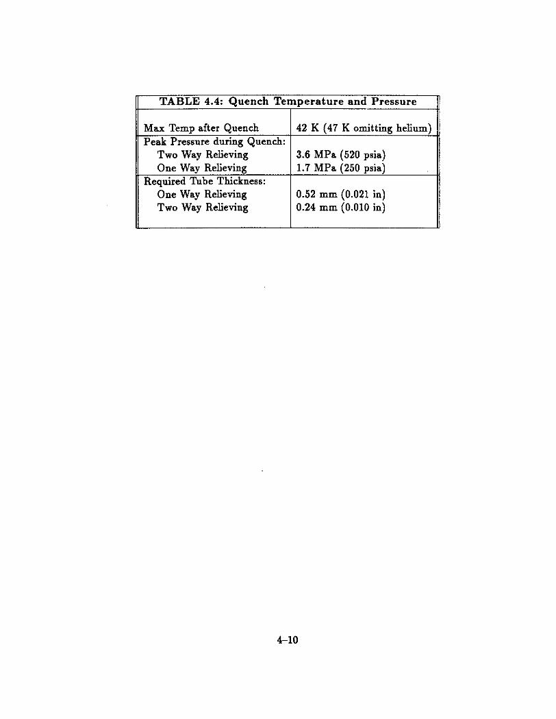
Max Temp after Quench 42 K (47 K omitting helium) Peak Pressure during Quench:

Two Way Relieving 3.6 MPa (520 psia) One Way Relieving 1.7 MPa (250 psia)

Required Tube Thickness: One Way Relieving 0.52 mm (0.021 in) Two Way Relieving 0.24 mm (0.010 in)

II TABLE 4.4: Quench TemDerature and Pressure

4-10

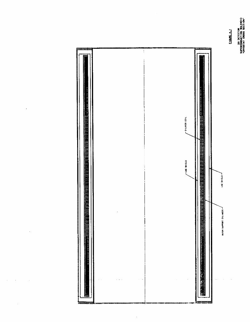
“k

d Jr

; g’[ ; 85

I 1

2 !; 6 2’ a 2 6% -- i

3c 8G 1 ssig . z

Epi kg* = 81;

25

,: j t , i x

vi

f z ‘/I T

I

/!!!I

II I/

‘::*:I’ ;I 2

.l’ s ;I I’ .,I > 1 y1

i

m

: m

55 2! a”

8:: * -

% ;f$ a:$

; Gg

2:

;:

7

-!-

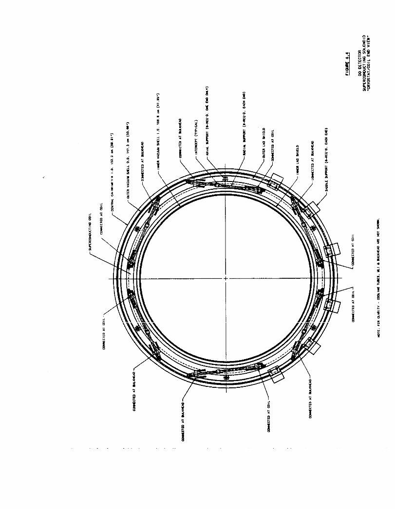
. i-

0. -G 2s f %fh EYS, a i-2 ; I i g$

,,~, ., ~,~,~,

B

I

I

c I

I

.,,~

E LHe out +

LHe in

il Axial Support Block

I Ill

- - -

Figure 4.5 Routing of liquid helium cooling tube on the support cylinder.

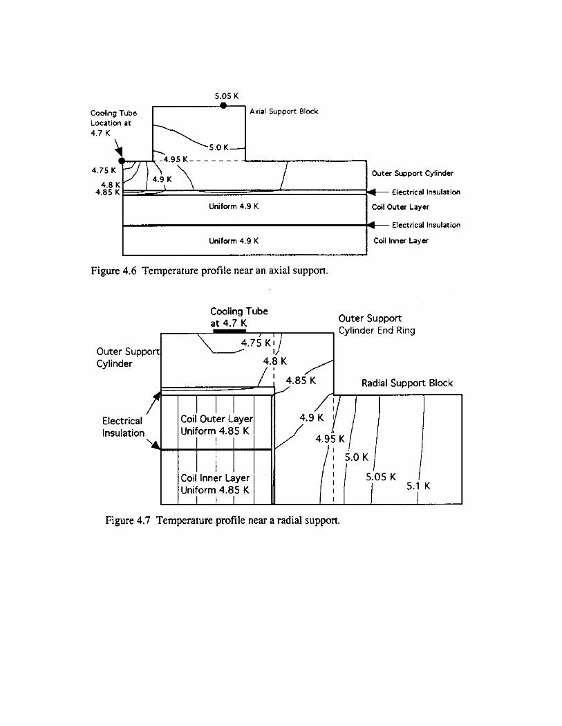
5.05 K

Cooling Tube -1 Axial S~pp~rf Block Locati& at 4.7 K t-l

Uniform 4.9 K

Uniform 4.9 K

Coil outer Layer

Electrical Insulation

Coil Inner Layer

Figure 4.6 Temperature profile near an axial support.

Cooling Tube at 4.7 K Outer Support

Cylinder End Ring

Outer Support Cylinder

/ Electrical Coil Ouier Layer\ Insulation Uniform 4.85 K 1

L.

Radial Support Block

I I

Coil Inner Layer I Uniform 4.85 K

I I I

Figure 4.7 Temperature profile near a radial support

0.2 0.2

5 5 go.15 go.15

E E .- .- ti ti 2 2 u) u) 0.1 0.1 : : E E 5 5 3 3 0.05 0.05 6 6

0 0

Flow Rate, g/s

Figure 4.8 Quality of helium leaving the cryostat as a function of mass flow rate of the helium.

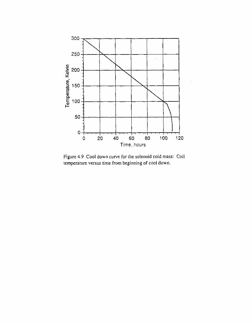
0 0 20 20 40 40 60 60 80 80 100 100 120 120 Time, hours Time, hours

250

2 2 150 iii

ho0 ?

\ .

Figure 4.9 Cool down curve for the solenoid cold mass: Coil temperature versus time from beginning of cool down.

70 70

60 60

z z 5 5 50 50 .E .E E E aj aj 40 40 E E

i=,30 i=,30

s s 8 8 20 20 cz cz

10 10

0 0 0 0 5 lb 10 1‘5 15 io 20 25 25 30 30 35 35 40 40 45 45 50 50

Temperature, Kelvin Temperature, Kelvin

Figure 4.10 Time for coil to reach 4.6 K from an elevated coil temperature.

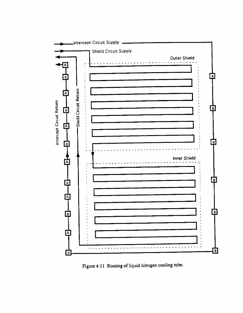
-Intercept Circuit Supply

Shield Circuit Supply

Outer Shield

j - I 1

I I i

I I ~

I i ‘i ,_ ___.______________________________I

Figure 4.11 Routing of liquid nitrogen cooling tube.

Inner Shield _______-______-__--______________;

1:

:::

I 1 :

I 1 :

I 1 0

I

I

I

I

I

il

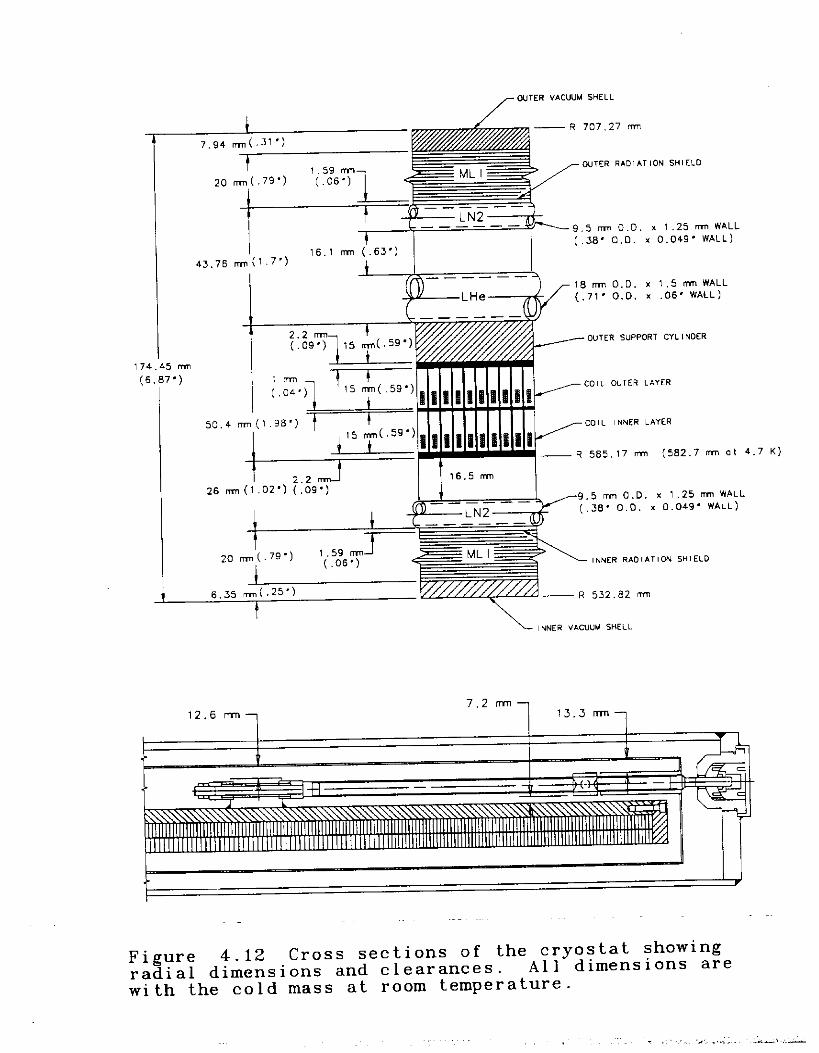
I __---- T--- -“- 16.1 mn (.63’1 e

(.X8’ 0.0. x 1 43.75 m(l.7’) I ---

Lk

I 174.45 lml (6.87’)

OUTER SUPPORT CYLlNOER

!

L.-O , !,< ,.!,‘~

COIL OUTER LII”ER

COIL INNER LAYER

R 585.17 m (582.7 mn ot 4.7 K) I I __ .,... I ~. ~~ , \... , 9.5 mm 0.0. x I .25 mn WALL

(.JB’ 0.0. x 0.049’ WALL)

12.6 m-n 1

Figure 4.12 Cross sections of the cryostat showing radial dimensions and clearances. All dimensions are with the cold mass at room temperature.

CHAPTER 5

SERVICE CHIMNEY

5.1 General

The service chimney is the vacuum insulated transfer line that carries the cryogenic and electrical services from the control dewar to the magnet cryostat. The insulating vacuum space of the service chimney serves as the relief line for the solenoid vacuum space, and pumpout of the magnet cryostat and control dewar vacuum spaces is done through the service chimney insulating vacuum space.

5.2 Routing

Figure 5.1 shows the path that the service chimney follows between the control dewar and the magnet cryostat. The pathway is severly constrained by existing detector elements. The chimney connects to a nozzle in the south bulkhead of the magnet cryostat at approximately the 4:00 o’clock location so that it can extend radially to the point at which it bends 90 degrees and proceeds south on a horizontal path.

The nozzle on the magnet cryostat bulkhead is a 152.4 mm (6 in) OD aluminum tube and the service chimney vacuum jacket has an aluminum to stainless transition near the bulkhead. At approximately 76 mm (3 in) south of the bulkhead, the service chimney turns east and makes a shape transition to a 76 mm (3 in) x 177.8 mm (7 in) obround shape for the span across the face of the CC cryostat. The vacuum jacket follows the curving contour of the south face of the CC on a path inclined downward approximately 27 degrees from the horizontal. The obround shape was chosen to fit in the available space between the CC and the south EC cryostats. The vacuum jacket makes a shape transition from the obround shape to a 22.9 cm (9 in) OD stainless steel tube at the outer edge of the EC where it turns and continues south once again. Along this path it runs horizontally through an area currently occupied by the south EC east cable trough. After a run of nearly 9 m (9.5 ft)it next turns eastward and upward at a 50 degree angle to the control dewar.

The chimney enters into the bottom of the control dewar and the vacuum pumping station is connected to the chimney just below the control dewar.

The chimney is supported along the face of the CC and at points along the 45 degree run. The length through the cable trough is kept clear to allow the cable trough to move south with the south EC when the detector is opened.

5-l

5.3 Vacuum Jacket

The vacuum jacket for the service chimney is designed for 0.044 MPa (6.4 psi) internal pressure and 0.207 MPa (30 psi) external pressure.

The obround length of the vacuum jacket was stress analyzed per ASME Section VIII Division 1, Appendix 13, “Vessels of Noncircular Cross Section.” The wall thickness for the obround is 4.8 mm (3/16 in). The maximum allowable internal or external working pressure was calculated to be 0.36 MPa (52 psi). The allowable stress used was reduced by 20% as required by Fermilab Environment, Safety, & Health rules for special pressure vessels [l]. The obround shape was also checked for buckling stability. It was concluded that the 0.36 MPa external pressure is less than l/10 of the critical external pressure that would cause collapse.

The 22.9 (9 in) type 304 stainless steel tube has a wall thickness of 3.18 mm (0.125 in). Per ASME code sections UG-27 and UG-28, it has an allowable internal working pressure of 2.48 MPa (360 psi) and an allowable external working pressure of 0.41 MPa (60 psi). The allowable stress used was reduced by 20% to (0.8) x (110 MPa) = 88 MPa.

5.4 Internal Contents

A layout of the internal contents of the service chimney in the obround section is shown in Figure 5.2. A layout of the chimney contents in the more traditional circular cross section for the remainder of the chimney is shown in Figure 5.3.

The first and last turns of the coil consist of doubled conductors which exit the winding and serve as the superconducting buses of the magnet. These buses are immediately attached to one side of the liquid helium supply tubing as it leaves the coil support cylinder. The arrangement of the buses and shape of the supply tubing in the obround section of the chimney was carefully chosen to minimize the thickness of the service chimney between the CC and EC calorimeters. The liquid helium supply tube is specially extruded for pressure service per ASTM-B-210 or ASTM-B-241. The tube in the obround portion is rectangular, 12.7 mm (0.50 in) x 31.8 mm (1.25 in) x 3.18 mm (0.125 in) wall. In the larger circular pipe portion of the transfer line, the tube is square, 31.8 mm (1.25 in) x 31.8 mm (1.25 in) with 19 mm (0.75 in) inside diameter. The MAWP of this tubing is estimated to be at least 11 MPa (1600 psi).

The two phase liquid helium return tubing is 19 mm (0.75 in) OD. x 1.65 mm (0.065 in) waII 6061-T6 aluminum. The MAWP for this tubing is 9.65 MPa (1400 psi). A 55 MPa (8.0 ksi) aUowable stress was used in calculating the MAWP’s.

There are separate liquid nitrogen circuits for the solenoid radiation shield and support intercepts. The shield circuit uses 12.7 mm (0.50 in) OD. x 1.65 mm (0.065 in) wall 6061-T6 aluminum tubing in the chimney. The support intercept circuit is of the same size but of 304 stainless steel material. These tubes have MAWP’s of greater than 13.8 MPa (2000 psi).

5-2

All four nitrogen tubes are thermally connected to the radiation shield. The chimney contains no instrumentation or voltage tap wires. The voltage tap leads

from the magnet terminals exit the bulkhead on the chimney end near the chimney nozzle. The leads run along the outside of the chimney vacuum jacket back to the control dewar area. An instrumentation port is located on the solenoid bulkhead opposite the chimney end for the remaining solenoid voltage tap and instrumentation leads.

5.5 Thermal Movement and Stress

The LHe and LN2 lines in the service chimney were analyzed for combined pressure, thermal movement, and dead weight. The tubing was stress analyzed per ASME code for Pressure Piping, standard ANSI/ASME B31.3, for the thermal cases shown in Table 5.1.

The commercial pipe stress analysis and design system by Algo@ [2] was used in the analysis. All stresses are well below code allowables. The locations for support of the LN2 tubing from the vacuum jacket walls are shown in Figure 5.4. Supports for the liquid helium lines are located as shown in Figure 5.5. The radial supports are of G-10 spider type guides that allow movement in the axial direction. The spider type supports are l/8 in thick as required to support a maximum reaction force of 290 N (65 lbf) in the direction orthogonal to the piping centerline. In addition to the spiders, line stops are located at points HE7b and TR7a to anchor axial movement of the tubing. The line stops are low heat leak design stainless steel wire cables which attach the helium tubing to the radiation shield and the nitrogen tubing to the vacuum walls.

The construction of the chimney is such that the LHe and LN2 lines are built with warm offsets at various locations so that the tubing can displace to a centered position during cryogenic operation. See Table 5.2 for a listing of the magnitude and locations of the built- in warm offsets. The LHe piping and LN2 piping have built in flexibility at the control dewar to allow for 2.0 cm (0.8 inches) of movement. Clearances are selected to be large enough to preclude thermal shorts due to thermal movement.

5.6 Fabrication and Location of Field Break

Because of the greatly restricted pathway of the obround portion of the service chimney great care must be taken to ensure that this portion of the vacuum jacket of the chimney will fit against the CC vacuum vessel correctly. Detailed measurements of the shape of the end of the CC vacuum vessel have been made so that a vendor can properly conform the vacuum jacket to the desired path. A checking fixture will be made using a casting technique on the actual CC head; this item will be used to check the contour of the obround section at the vendor’s.

A field break must be provided in the service chimney in the middle of the horizontal north-south section as shown in Figure 5.1, so that the control dewar and remaining attached

5-3

length of chimney can be installed in the detector. Likewise, the magnet cryostat and attached portion of chimney can be installed in CC if the chimney is parted as indicated. This parting of the chimney also facilitates shipping the system to Fermilab.

The major consequence of this requirement is that provisions for cutting and then rejoin- ing the superconducting buses in the chimney must be made. The chimney is temporarily closed out for full tests at the vendor’s. Then the chimney is severed for shipping and once again rejoined after the magnet and control dewar are installed in the DO detector. One approach might be to make the horizontal portion of the chimney overlong so that after the chimney is parted sufficient extra bus exists to make the field joint during installation.

Because alignment of the solenoid in CC is critical, some flexibility in the nozzle region of the chimney is desirable. A circumferential seam in the obround section near the nozzle may be left unwelded to permit small motions during final alignment as the magnet and chimney are installed. The inner contents of the chimney are sufficiently flexible to permit this motion. This seam can be temporarily sealed for the tests at the vendor’s and the chimney splinted to permit handling, and then fully welded after installation at Fermilab. Because the location of the control dewar is not so critical it can be adjusted a few centimeters as required while the field splice is made and no flexibility is required in the chimney at the control dewar end.

5.7 Heat Loads

The estimated heat loads for the chimney are listed in Table 5.3.

5.8 Vacuum Pumping and Relief Capacity

The chimney uses low emissivity aluminum tape [3] on the inside surfaces of the vacuum jacket, the surfaces of the radiation shield, and the LHe tubing. No multilayer insulation is used in the chimney in order to maximize the pumping path to the magnet cryostat vacuum space. Calculations show that the conductance of this space along the length of the chimney

exceeds 11 l/s helium at 300K at a pressure of 10e6 Torr. The small clearances between the radiation shield and the liquid helium tubes preclude the use of multilayer insulation in that volume.

The clear space in the chimney also serves as the magnet cryostat insulating vacuum relief venting path. With 0.122 MPa (17.7 psia) pressure at the solenoid and a 0.112 MPa (16.2 psia) vacuum lift plate at the control dewar, the relief venting path has 130 g/s helium or 300 g/s nitrogen capacity. That is well below possible failure mode flow rates for the two piping systems so rupture of either will not exceed the relieving capacity of the chimney.

5-4

5.9 Magnet Cryostat Nozzle

The routing of the cryogenic lines and superconducting buses from the chimney into the magnet cryostat through the cryostat nozzle is not expected to be trivial. The superconducting buses must be carefully anchored against motion in the magnetic field and must be everywhere thermally shorted to the helium supply tube while carefully isolated from it electrically. Custom transition pieces for the helium supply tubing are likely to be utilized in the nozzle region. A possible solution to the design problems this section of the chimney presents is indicated in Figures 5.6a, 5.6b, and 5.6~.

References

[l] It is conservative to follow Chapter 503ITA of the Fermilab ES&H Manual, which permits the use of a vessel fabricated in a shop that is not a Code Shop, provided the vessel is designed according to the ASME Boiler and Pressure Vessel Code rules, but where the Code allowable values of the maximum stress S (Div l.), or stress intensity S,,, (Div. 2), are reduced by the multiplicative factor 0.8.

[2] Algor, Inc., 150 Beta Drive, Pittsburgh, PA 15238-2932.

[3] E.M.W. Leung, et. af, “Techniques for Reducing Radiation Heat Transfer Between 77 and 4.2 K”, Advances in Cryogenic Engineering, Vol. 25, Plenum Press, New York (1980), p. 489.

5-5

, rable 5.1: Stress Analysis Thermal Cases Case 1 LN2 Line 1 LHe Line / Solenoid

I I

1 Warm Cold 2 Warm Cold 3 Warm Warm 4 Cold Cold 5 Cold Cold 6 Cold Warm 7 Cold Warm 8 Warm Warm

-

Location

TR6 TR7

HE6 HE7

Table 5.2: Built-In Offsets For

$0.97 cm - -0.90 cm -

Warm Cold Cold Cold

Warm Cold

Warm Warm

‘hermal Movement “2” Offset

-

+0.74 cm

-

$0.74 cm

Table 5.3: Heat Loads for the Chimney Item 1 300 K to 80 K 1 80 K to 5 K

I Radiation, Obround Section 13.6 W 123 mW Radiation, Circular Section 86.4 W 780 mW Field Joints - 100 mW Conduction (Spiders) 7.6 W 440 mW

Total 108 W 1.5 w

5-6

w

W

+

I3

8

g[-- -~kG-zE~ ,,$N EF sum lrn m

(IIt PDYD mJlllDl, ,,’ J il--.--,, 111 1 _-_____ -__--- w c:I=:I=I3 cz---- ---

r

F

___

/ ~WTER&3IDI poI”T

_____-- .-----

~ISl.S1S- ---__--- -_----

&I -------- ~--- _--_---- -_-- ----- 1 I=

-_--_ ----- PLAN VIEW

I ~---~-- -__---__, -I 7 _______ -__---

STAT I - /- -&%P ES

-__----- --~-~- ! T’ -x, ._. ,. t J + ,... ,... -_

-

,__

t-

r --A.. ~,02.~~

CUTAWAY LOOKING NORM

1 T L

Figure 5.1 Chimney Routing

3 : 2

2

i .- :

T

s 8 N d

F zl ‘L

c 2 G -

iiT

k .- L 0

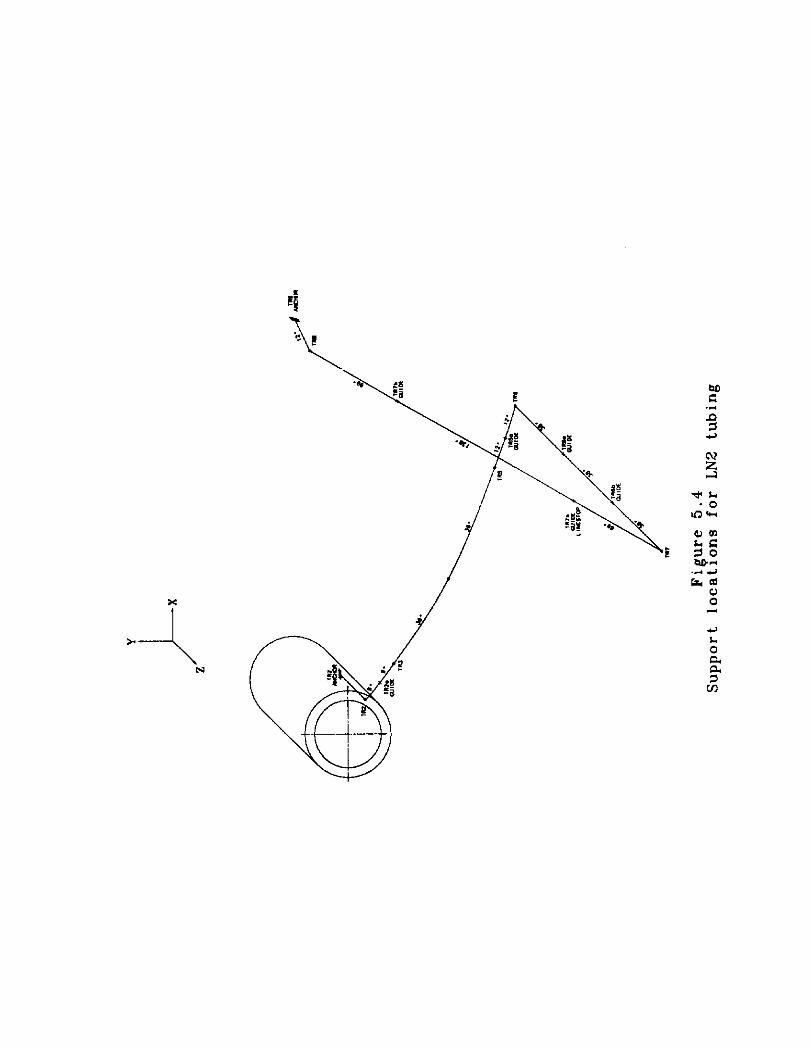
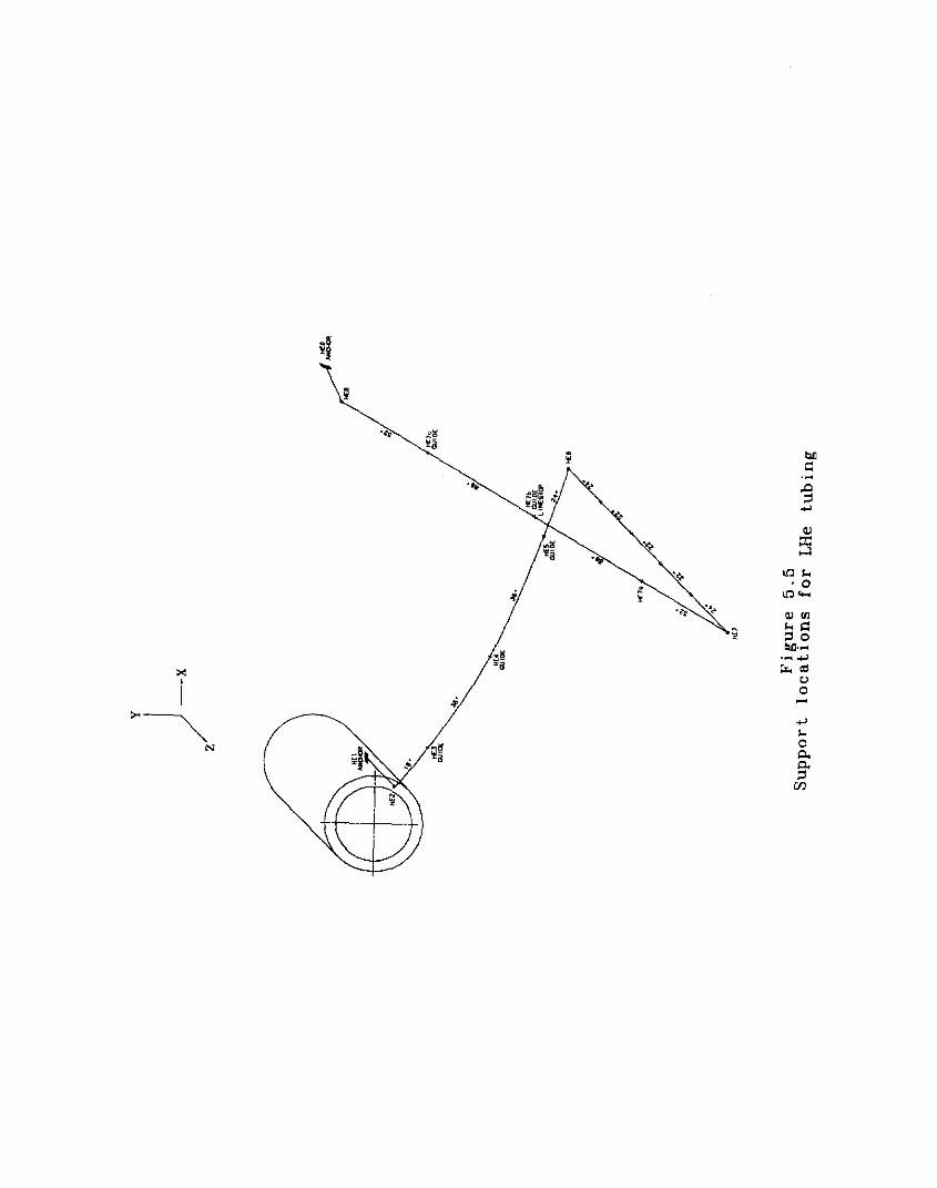
e” .d

T 4

aJ

3

LOL

lct2

$2

M.4 .- c, ram

0”

4

t--------+

I

- - - -7-r 6 .&z *p = = 9 - f < :*-\\,--- s- -.A*= --_c -,-_==

$

53-y - .z?- .u. zz-AL -

11 ~..A,.. /

CHAPTER 6

CONTROL DEWAR

6.1 General

The control dewar is the interface between the permanently installed building piping and the moveable detector. It has bayonet connections for cryogenic lines and contains the vapor- cooled current leads. It also contains a liquid helium reservoir, a LHe supply line subcooler, a LHe supply J-T valve and other required valving and instrumentation. Instrumentation required in the control dewar is detailed in Chapter 9. The control dewar is physically 0.81 m (32 in) in diameter and approximately 1.5 m (60 in) tall. It weighs about 450 kg (1000 lbs).

A schematic of the control dewar is shown in Figure 6.1. The penetrations in the control dewar are tabulated in Table 6.1. A layout of the top head of the control dewar is shown in Figure 6.2, and the configuration of key internal components is shown in Figure 6.3.

There are no penetrations through the shell portion of the vacuum vessel. This feature permits straightforward assembly of the internal components of the dewar with final closeout obtained by sliding the vacuum shell over the two torospherical heads and joining it to them with single fillet lap welds. Struts can maintain the spacing of the heads before the shell is installed. This design feature also permits access to the internal contents of the control dewar in the event a repair is required, by removal of the fillet weld which joins the heads and the shell and lifting the shell vertically off. The liquid nitrogen cooled radiation shield is constructed with joints that allow it to be removed after making cuts in the liquid nitrogen tubing.

The location for all but one of the aluminum to stainless steel material transition joints in the cryogenic lines in the service chimney is located just below the control dewar. The chimney vacuum jacket has a sleeve that will be slid up and welded once the joints are complete. Table 6.2 lists the locations of the material and shape transitions for the control dewar and chimney cryogenic lines.

6.2 Mounting and Access

The control dewar is located outside the detector, mounted on an access platform to be attached to the existing detector cryo utilities bridge at an elevation corresponding to the top access level of the muon truss. Access to the control dewar platform is made by ladder from the detector platform below it during normal operations when the CF toroid is closed. When

6-l

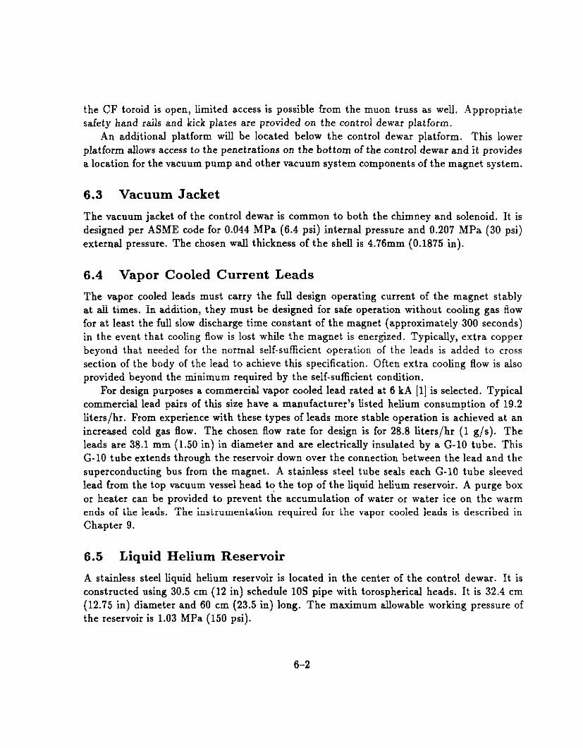
the CF toroid is open, limited access is possible from the muon truss as well. Appropriate safety hand rails and kick plates are provided on the control dewar platform.

An additional platform will be located below the control dewar platform. This lower platform allows access to the penetrations on the bottom of the control dewar and it provides a location for the vacuum pump and other vacuum system components of the magnet system.

6.3 Vacuum Jacket

The vacuum jacket of the control dewar is common to both the chimney and solenoid. It is designed per ASME code for 0.044 MPa (6.4 psi) internal pressure and 0.207 MPa (30 psi) external pressure. The chosen wall thickness of the shell is 4.76mm (0.1875 in).

6.4 Vapor Cooled Current Leads

The vapor cooled leads must carry the full design operating current of the magnet stably at all times. In addition, they must be designed for safe operation without cooling gas flow for at least the full slow discharge time constant of the magnet (approximately 300 seconds) in the event that cooling flow is lost while the magnet is energized. Typically, extra copper beyond that needed for the normal self-sufficient operation of the leads is added to cross section of the body of the lead to achieve this specification. Often extra cooling flow is also provided beyond the minimum required by the self-sufficient condition.

For design purposes a commercial vapor cooled lead rated at 6 kA [l] is selected. Typical commercial lead pairs of this size have a manufacturer’s listed helium consumption of 19.2 liters/hr. From experience with these types of leads more stable operation is achieved at an increased cold gas flow. The chosen flow rate for design is for 28.8 liters/hr (1 g/s). The leads are 38.1 mm (1.50 in) in diameter and are electrically insulated by a G-10 tube. This G-10 tube extends through the reservoir down over the connection between the lead and the superconducting bus from the magnet. A stainless steel tube seals each G-10 tube sleeved lead from the top vacuum vessel head to the top of the liquid helium reservoir. A purge box or heater can be provided to prevent the accumulation of water or water ice on the warm ends of the leads. The instrumentation required for the vapor cooled leads is described in Chapter 9.

6.5 Liquid Helium Reservoir

A stainless steel liquid helium reservoir is located in the center of the control dewar. It is constructed using 30.5 cm (12 in) schedule 10s pipe with torospherical heads. It is 32.4 cm (12.75 in) diameter and 60 cm (23.5 in) long. The maximum allowable working pressure of the reservoir is 1.03 MPa (150 psi).

6-2

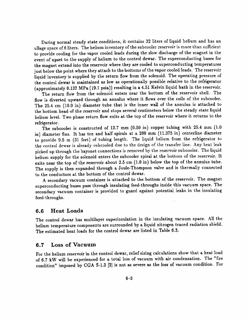
During normal steady state conditions, it contains 32 liters of liquid helium and has an ullage space of 6 liters. The helium inventory of the subcooler reservoir is more than sufficient to provide cooling for the vapor cooled leads during the slow discharge of the magnet in the event of upset to the supply of helium to the control dewar. The superconducting buses for the magnet extend into the reservoir where they are cooled to superconducting temperatures just below the point where they attach to the bottoms of the vapor cooled leads. The reservoir liquid inventory is supplied by the return flow from the solenoid. The operating pressure of the control dewar is maintained as low as operationally possible relative to the refrigerator (approximately 0.132 MPa (19.1 psia)) resulting in a 4.51 Kelvin liquid bath in the reservoir.

The return flow from the solenoid enters near the bottom of the reservoir shell. The flow is diverted upward through an annulus where it flows over the coils of the subcooler. The 25.4 cm (10.0 in) diameter tube that is the inner wall of the annulus is attached to the bottom head of the reservoir and stops several centimeters below the steady state liquid helium level. Two phase return flow exits at the top of the reservoir where it returns to the refrigerator.

The subcooler is constructed of 12.7 mm (0.50 in) copper tubing with 25.4 mm (1.0 in) diameter fins. It has ten and half spirals at a 289 mm (11.375 in) centerline diameter to provide 9.5 m (31 feet) of tubing length. The liquid helium from the refrigerator to the control dewar is already subcooled due to the design of the transfer line. Any heat leak picked up through the bayonet connections is removed by the reservoir subcooler. The liquid helium supply for the solenoid enters the subcooler spiral at the bottom of the reservoir. It exits near the top of the reservoir about 2.5 cm (1.0 in) below the top of the annulus tube. The supply is then expanded through a Joule-Thompson valve and is thermally connected to the conductors at the bottom of the control dewar.

A secondary vacuum container is attached to the bottom of the reservoir. The magnet superconducting buses pass through insulating feed-through6 inside this vacuum space. The secondary vacuum container is provided to guard against potential leaks in the insulating feed-throughs.

6.6 Heat Loads

The control dewar has multilayer superinsulation in the insulating vacuum space. All the helium temperature components are surrounded by a liquid nitrogen traced radiation shield. The estimated heat loads for the control dewar are listed in Table 6.3.

6.7 Loss of Vacuum

For the hel&n reservoir in the control dewar, relief sizing calculations show that a heat load of 6.7 kW will be experienced for a total loss of vacuum with air condensation. The “fire condition” imposed by CGA S-l.3 (21 is not as severe as the loss of vacuum condition. For

6-3

loss of vacuum a relief set at 1.03 MPa (150 psi) with a flow rate of 130 SCFM air will safely protect the helium reservoir against loss of vacuum.

References

[l] American Magnetics Inc., PO Box 2509, 112 Flint Road, Oak Ridge, Term 37830

[2] CGA S-l.3 Pressure Relief Device Standards, Compressed Gas Storage Containers, Com- pressed Gas Association, 1235 Jefferson Davis Hwy, Arlington, Va, 22202.

6-4

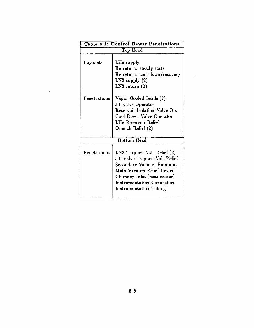
Bayonets LHe supply He return: steady state

He return: cool down/recovery LN2 supply (2) LN2 return (2)

Penetrations Vapor Cooled Leads (2) JT valve Operator Reservoir Isolation Valve Op. Cool Down Valve Operator LHe Reservoir Relief Quench Relief (2) I

I

Bottom Head

Penetrationt LN2 Trapped Vol. Relief (2) JT Valve Trapped Vol. Relief Secondary Vacuum Pumpout Main Vacuum Relief Device Chimney Inlet (near center) Instrumentation Connectors

II

Instrumentation Tubing

-I

Table 6.1: Control Dewar Penetrations Top Head

6-5

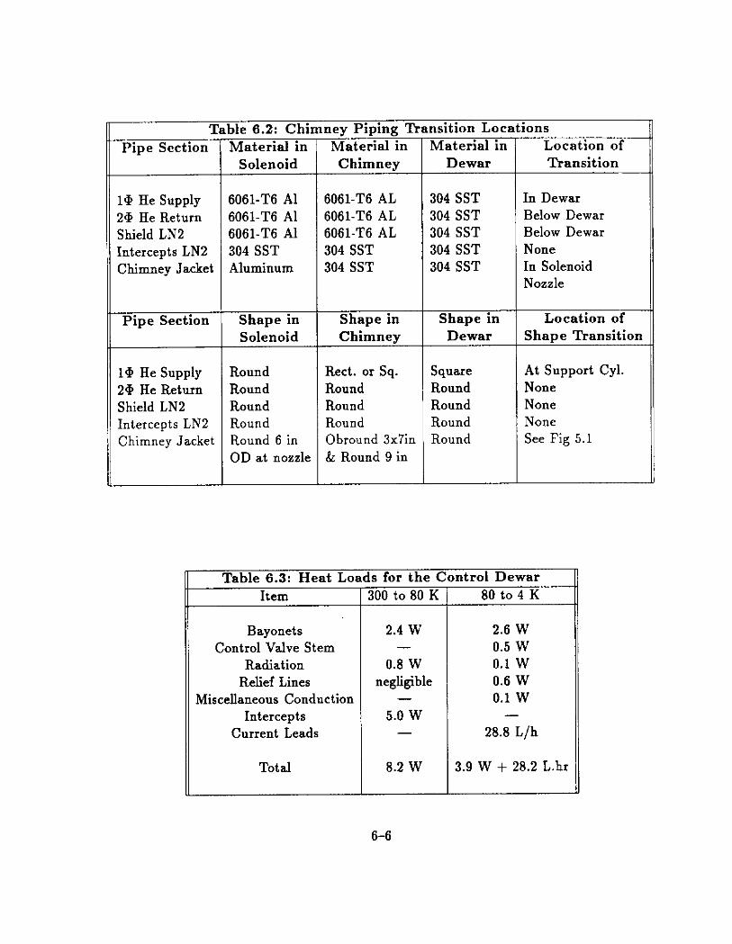
1: Pipe Section

ble 6.2: Chimnev PiDine Transition Locations Material in

Solenoid

la He Supply 6061-T6 Al 2+ He Return 6061.T6 Al Shield LN2 6061-T6 Al Intercepts LN2 304 SST Chimney Jacket Aluminum

Pipe Section

l@ He Supply 2+ He Return Shield LN2 Intercepts LN2 Chimney Jacket

n

Shape in Solenoid

Round Round Round Round Round 6 in OD at nozzle

Chimney

6061-T6 AL 6061-T6 AL 6061-T6 AL 304 SST 304 SST

Shape in Chimney

Rect. or Sq. Round Round Round Obround 3x7in & Round 9 in

Material in Dewar

304 SST 304 SST 304 SST 304 SST 304 SST

Shape in Dewar

square Round Round Round Round

Location of Transition

i.

In Dewar Below Dewar Below Dewar None In Solenoid Nozzle

Location of Shaue Transition

At Support Cyl. None None None See Fig 5.1

Table 6.3: Heat Loads for the Control Dewar Item 1 300 to 80 K / 80 to 4 K

Bayonets 2.4 W Control Valve Stem -

Radiation 0.8 W Relief Lines negligible

Miscellaneous Conduction -

Intercepts 5.0 w Current Leads -

2.6 W 0.5 w 0.1 w 0.6 W 0.1 w

28.8 L/h

Total I

8.2 W 3.9 W + 28.2 L.hr

6-6

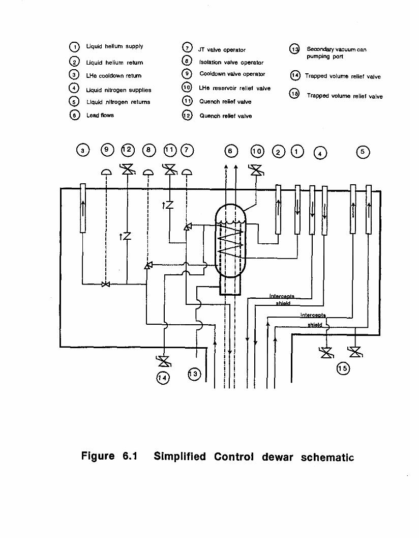
0 Quid helium SUPPLY

0 Uquid helium return

0 LHe cooldown return

0 JT vs,ve opera,or

lsolatlon valve operator

Cooldown valve operator 0 14 Trapped volume relief valve

g tiquid ni,,ogen supplies

5 Liquid nitrogen returns

@ LHe reservoir relief valve

0

0 TwP~~ volume relief valve

Quench relief valve

(3 Lead fkwa Quench reliif valve

1

?

t f I I I I I I I

$

I

.i i ! i I i i i i i i i i i i i i i i i i i i i i i i i i

Figure 6.1 Simplified Control dewar schematic

LHe supply bayonet @ LN2 retwn bayonet 0 11 lsolatlan Valve operator

0 LHe ret”m bayonet 0 LN2 return bayonet 0 ,2 Cooldown valve operator

Llie cooklown return bayonet head now 00nmn 0 t3 LHe reservoir relief valve

LN2 supply bayonet Lead fknv connection @ Cluench relief valve

LN2 supply bayonet JT valve operator @ Quench relief valve

V-VALVE OPERATOR

Figure 6.2 Control dewar top head layout

(not to scale)

Ia. Lo JT *oh.

LE. “,““I lrorn u**nc.M

LM. .uo#Y to .d.dd

*“o.-d”daI

/

La. ,.l”,” 1s ,.triq.rsLor

/-

w1 R~a*tlc.n .h!dd

A---- -NYm San /- s’rdn ‘-I-

> < /’ / /

/ /

---

-

/

“c&““rn .h.ll

Figure 6.3 Cross section of Control dewar

CHAPTER 7

REFRIGERATION SYSTEM

7.1 General Requirements

The D0 solenoid system will require a cryogenic refrigeration system to supply LN2 and LHe to the magnet. In addition to the magnet, a Visible Light Photon Counter (VLPC) system with liquid helium cryostats~will also be added to the upgraded detector. The two new systems will operate simultaneously and are thus considered together in designing the required retigeration system needed for the upgraded detector.

An existing cryogenic system at DO supplies LN2 refrigeration to the three existing liquid argon calorimeter cryostats of the detector and provides for storage of pure liquid argon required by the calorimeters. An existing control system enables the automatic operation of the calorimeter cryostats at fked pressure and liquid argon level.

Economic and operational considerations indicate that and upgrade/modification of the existing D0 cryogenic system is most appropriate. An existing LN2 dewar storing 75.7 kl LN2 has adequate capacity for the liquid nitrogen needs of the magnet cryostat, the VLPC cryostats, and a helium refrigerator/liquitier of adequate capacity.

A standard Fermilab satellite STand &lone Refrigerator (STAR) will be installed to provide the helium refrigeration required. The capacity of the STAR is sticient for nonsi- multaneous cooldown and simultaneous operation of both the solenoid and VLPC systems. The STAR refrigerator will make LHe into a 2000 L storage dewar. This dewar will supply liquid via separate transfer lines to the magnet control dewar and the VLPC cryostats.

7.2 Building Requirements

There is adequate space in the DO Assembly Building (DAB) to house the STAR expansion engines, heat exchanger, helium storage dewar, and valve box.

An annex will be added to the existing DO Tevatron compressor building to house two additional Mycom compressors; the mass flow from one compressor will be allocated to the DO STAR and the other compressor will serve as an on-line spare for either D0 or the Tewtron. Additional helium purifk equipment will be installed at the compressor building annex for the added Mycom compressors.

7-1

7.3 Flow Diagram

A simple box diagram of the rekigerator system is shown in Figure 7.1 and the corresponding simplified flow diagram is shown in Figure 7.2.

7.4 Hardware Components

The hardware components that make up the new LHe refrigerator system are the compressors, a heat exchanger, expansion engines, a valve box, a LHe storage dewar, transfer lines, and a solenoid (including the service chimney and control dewar).

7.4.1 Compressor

The two 400 HP two-stage IVycorn compressor to be installed for the D0 refrigeration system are identical to those used in the Tevatron. They are specified to provide 50 g/s helium at a discharge pressure of 20 atms, but measurements show they typically provide 57 g/s mass flow. Two standard full-flow three stage purifiers will also be installed with the compressors to remove oil and water from the discharge helium. Piping in the DO compressor building annex will permit the eventual connection of the compressors into the Tevatron helium system. The discharge and suction lines of the DO compressors run across the Tevatron berm to DAB; a dirty gas return line and inventory management line are provided to a helium butfer tank near DAB. The system is very similar to the system presently used at the Tevatron, and in particular to the STAR used at the collider detector facility at BO.

7.4.2 Heat Exchanger

The STAR heat exchanger is a horizontal vacuum vessel containing the LN2/He and He/He heat exchangers. It will be located in the DAB assembly hall.

7.4.3 Expansion Engines

The STAR uses a dry reciprocal expansion engine across the process stream and a wet reciprocal expansion engine in the process stream. These engines are provided in individual vacuum vessels and connect to the heat exchanger with U-tubes. They wiil be located near the heat exchanger in the DAB assembly hall. These expansion engines are used throughout Fermilab and there are available spare engines in case of failure or other severe problems.

7.4.4 Valve Box

A valve box serves as a junction between the heat exchanger, wet engine, storage dewar and transfer line with interconnections made with U-tubes. It is a vacuum box with external bayonet fittings and valve operators and internal cold piping and valves. The box containr

7-2

two control valves: the high to low pressure bypass valve and a J-T valve in par&l with the wet engine. The valve box will be located near the expansion engines and heat exchanger in DAB.

7.4.5 Storage Dewar

The STAR refrigerator will make LHe into a 2000 L storage dewar. This dewar will be a commercially procured ASME Boiler and Pressure Vessel Coded dewar with an MAWP of 7 atmospheres. The pressure rating is appropriate for pressures encountered during quenches and cooldowns. In the steady-state condition the dewar will operate at 1.8 atm, 4.9K which will be the driving pressure of the ffow through the magnet. The storage dewar will be located in DAB near the expansion engines.

7.4.6 Transfer Line

U-tubes will connect the storage dewar, heat exchanger and LN2 header to the LN2/LHe/GHe transfer lines. One transfer line will deliver cryogens to the detector standby position in the Assembly Hall and another will deliver cryogens to the Collision Hall. U-tubes connect the transfer line to the magnet system control dewar.

7.4.7 Control Dewar and Solenoid

The control dewar is described in Chapter 6. It is the interface between the permanently installed cryogenic building piping and the service chimney and solenoid mounted on the moveable detector.

7.5 System Heat Loads and Capacity

A detailed description of the low temperature components and the identified heat loads to the LN2 and LHe systems are given in Table 7.2. The total identified steady state helium heat load is approximately 40 W plus 28.8 L/hr with an additional 20 W during charging. The nitrogen heat load is approximately 241 W equivalent to approximately 5.4 L/hr.

Figure 7.3 shows the nominal capacity of the STAR refrigerator with the identified and expected heat loads. It can be seen that there is adequate refrigeration to handle the heat load from both the magnet system and the VLPC system.

7.6 Refrigerator Control System

The refrigerator/compressor control system will be supported by the existing DO cryogenic control system. The control system is described in chapter 9.

7-3

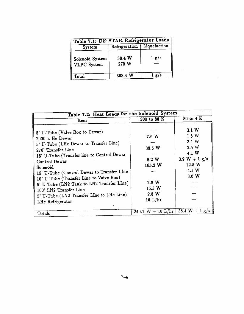
Table 7.1: DO STAR Refrigerator Loads System 1 Refrigeration 1 Liquefaction

I

Solenoid System 38.4 w 1 ix/s VLPC System 270 w -

I / Total 308.4 W 1 g/s H

Table 7.2: Heat Loads for the Solenoid System Item 300 to 80 K

I

5’ U-Tube (Valve Box to Dewar) 2000 L He Dewar 5’ U-Tube (LHe Dewar to Transfer Line) 270’ Transfer Line 15’ U-Tube (Transfer line to Control Dewar Control Dewar Solenoid 15’ U-Tube (Control Dewar to Transfer Line 10’ U-Tube (Transfer Line to Valve Box) 5’ U-Tube (LN2 Tank to LN2 Transfer Line) 100’ LN2 Transfer Lime 5’ U-Tube (LN2 Transfer Line to LHe Line) LHe Refrigerator

Totals

-

7.6 W -

38.5 W -

8.2 W 165.3 W

-

2.8 W 15.5 w 2.8 W

10 L/hr

240.7 W + 10 L/hr

I

80 to 4 K

3.1 w 1.5 w 3.1 w 2.5 W 4.1 w

3.9 w + 1 g/s 12.5 W 4.1 w 3.6 W

- - - -

38.4 W c 1 gJs

7-4

,

, I I I I I

:

I

! _--____- 2 __-_---------- I

I I I I I I TLV VLPC

-

C \, - HTX

FIGURE 7.1: Refrigeration System - Box Diagram

Symbols: N=liquid nitrogen tank; Csompressor; ST=storage / buffer tank;

HTX=heat exchanger; GE=gas expansion engine; LE=liquid

expansion engine: VB=value box; D=LHe dewar; TLM=transfer

line for magnet; CD=control dewar; Mzmagnet; TLV=transfer line

line for VLPC cryostat; VLPC=VLPC cryostat

I ~~~~ -” 6 3 1

1 iI..I:~Qj %, rm7 1 I ; I’& v ~~~ 64-i

ev z

L

7 ; F r ;

2” a

F’

ro L--l J

2 f ; TX; Q

Cl

::. ,5

z 01 0

z % 2 ; 5

$ x

If

2 -I -- -I

z _ - z

L

Valve Legend

Heat Exchanger LN2 Control Valve HXl Flow Control Valve HX2 Flow Control Valve Dry Engine Flow Control Valve Wet Engine Flow Control Valve J-T Valve Bypass Valve Storage Dewar Pressurizing Valve Control Dewar Pressurizing Valve Magnet Flow Control Valve (J-T Valve) Cool-down Valve Vapor Cooled Lead Flow Control Valve Solenoid Valves for Open Cycle Operation Suction Side Inventory Control Valve Discharge Side Inventory Control Valve 1st Stage Slide Valve Compressor Bypass Valve Interstage Slide Valve Clean Gas Supply Valve Dirty Gas Discharge Valve Magnet LN2 Control Valves VLPC Cryostat Control Valves VLPC Nitrogen Control Valve

Vl v2 v3 v4 v5 V6 V7 V8 v9 VlO Vll V12,13 v14,15 V16 v17 V18 v19 v20 v21 v22 V23,24 V25,26 v27

Figure 7.2b

25 - 25 -

100 100 200 200 3ocl 3ocl Jo0 Jo0 500 500 600 600

Refrigeration Refrigeration - - W W

Figure 7.3: Capacity of star refrigerator and (1) identified steady state

heat load, (2) max. expected charging heat load

CHAPTER 8

VACUUM SYSTEM

8.1 General

An existing vacuum facility is installed on the DO detector platform which provides a utility vacuum header and an insulating vacuum header to the calorimeters on the platform. The utility header is used for general purpose vacuum pumping procedures such as pumping and purging. It is connected to a gas manifold that allows backfilling with low pressure dry nitrogen. The insulating vacuum header is a dedicated pumping path for the liquid argon calorimeter insulating vacuums. The magnet system and refrigerator can make use of either of the pumping headers keeping the intended purpose of each the same.

The vacuum pumps for the existing system are housed in a pump room that is accessible at all times. A portion of the current piping schematic showing these pumps is shown in Figure 8.1. The vane pumps [l] are double stage rotary vane vacuum pumps with a nominal pumping speed of 100 l/s. The blower [2] 1s a Roots-type pump with a nominal pumping speed of 500 l/s.

8.2 Insulating Vacuum

A simplified schematic for the solenoid vacuum system is shown in Figure 8.2 For initial cleanup and pumpdown of the magnet insulating vacuum or other operations where conditions would interfere with calorimeter insulating vacuum pumping, the utility vacuum header will be used. Pumpdowns from atmospheric will be throttled to prevent damage to multilayer insulation in the control dewar vacuum space. For normal operations the insulating vacuum header will be used. After the control dewar and solenoid insulating vacuum is at the lowest attainable pressure it will be isolated. A turbomolecular pump will be provided between the isolation valve and the vacuum pumping system. The turbomolecular pump is mounted locally on the platform below the control dewar, outside the magnetic fields which could interfere with its operation.

The primary pumping path for the magnet insulating vacuum space is through the chimney in the clear space between the liquid nitrogen shield and the vacuum jacket. The effective pumping speed at the solenoid and control dewar are larger than that required to keep the solenoid operating should a small leak appear. The conductance of the pumping path was calculated for the free molecular flow regime and it was determined that for a turbomolecular pump with a nominal pumping speed of 1000 l/s, the effective pumping speed at the solenoid

8-l

will be greater than 8 l/s. The required pumping speed at the solenoid to maintain the coil at 2 x IOe7 Torr with a warm 1 x 10-s atm-cc/set leak leaking cold LHe is 4 l/s.

8.3 Electrical Feedthroughs and Secondary Vacuum Container

Dielectric breaks in the form of ceramic electrical feedthroughs are required where the superconducting buses for the magnet penetrate the subcooler helium reservoir in the control dewar. A secondary vacuum container is provided to guard against unintended helium leaks in these rather fragile elements. A separate pumping line for this secondary vacuum container is provided which is independent from the system insulating vacuum. During initial pumpdown this line is connected to the inlet of the turbomolecular pump; during normal operation the secondary vacuum container is isolated. In the event of a small leak in one of the feed&roughs alternate pumping arrangements for the secondary vacuum container can be arranged.

References

[l] Edwards model E2M275, Edwards High Vacuum International, 301 Ballardvale Street, Wilmington, MA 01857

[2] Leybold Ruvac model SU2000, Leybold Vacuum Products, Inc. 5700 Mellon Rd, Export, PA 15632-8900

8-2

‘r

I

I-’ I I I i

I I

!

I

i

!

i

I

f I f I f I

4.

I

.‘/ !%

; I I I I I

f I I I f I I I

I !I I

f I I I

i .-1

i 1

(-- t

(Z + I

I “r

I ----------------------------- (‘11s NOEW3) 3SP9 .C

A------.-----

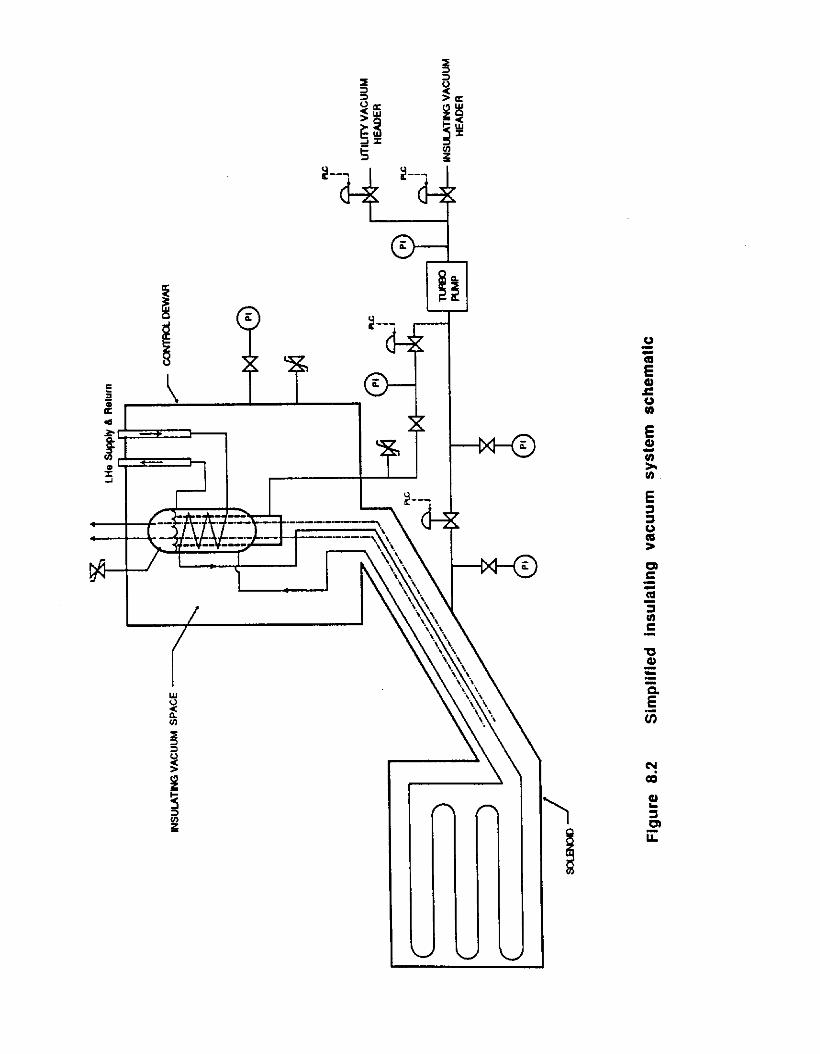
3 I -2-L I-71 _ me- - : -.- - _-wme.e.\ --.- -- Jqgm+ ---? “, v--v--- -1 -

\\ . . . . I ‘XV\ \ \ i I

1 ” w+ \ \ z \ \. \ \. \. \. / \. \ x. \.

I I 1 \ \ ‘\,..< \

E 2 ! E 1 2 2 c $ = = E z

CHAPTER 9

CONTROL AND INSTRUMENTATION

9.1 Overview

An existing Texas Instruments TI565T Programmable Logic Controller [l] (PLC) provides control and monitoring of the liquid argon cryogenics system, three detector gas systems, and all of the cryogenic subsystems (e.g. vacuum, compressed air, the Oxygen Deficiency Hazard warning system, and the glycol cooling system) of the existing DO detector. The PLC provides automatic control and operator manual intervention for all controlled elements as desired, and graphical display and data logging of all monitored parameters when required. The system will be expanded to control and monitor the VLPC, solenoid, and helium refrigerator systems.

A Texas Instruments T1555 PLC will be added to the existing PLC system to control and monitor the magnet power supply and protection switch and to log fast and slow data from the magnet instrumentation. A hardwired chassis and logic unit making up a quench protection monitor (QP,M) will provide primary quench protection for the magnet.

A variety of instrumentation and sensors from the magnet and refrigeration system provide signals for the PLC’s and the hardwired protection unit.

9.2 Existing PLC System

The existing DO PLC system is a stand alone system with an internal battery backed program memory which requires no host system to download the control programs in the event of a power failure. It consists of two independent TI565T processors operated in a “hot backup” configuration. One PLC is on line and actively controlling the system; the second is in standby running step for step with the on line unit but with its input/output communication disabled. Each PLC runs continuous internal diagnostics for errors. When a fatal error is registered by the active PLC, the hot backup option takes it offline and puts the standby PLC online without intervention or disruption to the system. The existing control system configuration is shown ~schematically in Figure 9.1, with added elements for the magnet system, the VLPC system, and the helium refrigerator indicated. The specifications for the TI565T are given in Table 9.1.

9.2.1 PID Loop Control

The T1565 PLC is provided with 64 preconfigured feedback PID (proportional, integral, differential) process control loops. The 25 existing loop assignments plus those to be added

9-l

for the VLPC system, the helium refrigerator, and the magnet are shown in Table 9.2. The PLC is capable of advanced control loop features such as feed forward or cascade control if needed.

9.2.2 DMACS

Distributed Manufacturing and Control Software - DMACS - is the operator control interface software for the PLC. DMACS provides the graphical control environment through which operators can monitor and control any process variable I/O connected to the PLC and defined in its data base. Floating-point math and high level programming with the Special Function programming language are available. All control interfaces and menus are pass- word protected by DMACS to prevent unauthorized operation of the systems to which they pertain. The speci%ations for the DMACS system, and the tasks supported by DMACS at DO are presented in Table 9.3.

9.3 System Instrumentation

The VLPC system, the helium refrigeration system, and the magnet system will add a substantial number of channels of instrumentation which will be monitored by the upgraded PLC; certain of these channels will also be monitored by the hardwired QPM. Th,at required for the VLPC system is not considered further herein. For the helium refrigeration system, magnet system, and magnet energization system a number of device types will be present, including valve position transducers, temperature sensors, voltage taps, expansion engine speed sensors, flow rate sensors, and vapor pressure and absolute pressure devices.

9.3.1 Thermometry

The helium refrigeration system and the magnet system will utilize three different types of thermometry devices: platinum [2] and carbon-glass [3] RTD’s, and VPT’s [4]. The RTD’s can be accessed directly by the PLC; The VPT’s will require a pressure transmitter to interface to the PLC.

An extensive set of RTD thermometry is required for the magnet coil and cryostat, and for the helium subcooler reservoir and vapor cooled leads in the magnet control dewar. Much of the thermometry in the magnet cryostat is provided to monitor cooldown, to verify the performance of the radiation shield and cold mass support systems, and to provide for the permit to charge up the magnet or to trigger a discharge in the event abnormal temperatures are detected. The thermometry in the control dewar is provided to assist cooldown and to protect the vapor cooled leads by detecting abnormalities. Table 9.4 presents the thermometry list of the TI565T for the magnet system.

9-2

Temperature sensors are provided for the power supply water cooled diodes to ensure that they are operating properly. Temperature sensors in the balance of the energieation system are provided to indicate proper conditions prior to energization of the magnet.

9.3.2 Potential Taps

Potential taps on the magnet coil and superconducting buses, vapor cooled leads, and remainder of the energization system are required to safely operate the system. A coil center tap plus taps at each input bus of the magnet, plus one additional tap at the quarter point on one half of the coil comprise the potential taps for the magnet. Bridge configurations which compare the voltage unbalances between various portions of the coil will signal the presence of a normal zone and generate a quench detection trigger. Additional potential taps are required at the top and bottom of the vapor cooled leads and on the reversing switch, protection resistor, and power supply to provide additional monitoring of the status of the these components. Additional details concerning the energization system are presented in Chapter 10.

9.3.3 Other Sensors

The balance of the helium refrigeration system will provide valve position sensors, pressure transducers, flowrate meters, and expansion engine speed indicators. Many of these are implicit in the PID loop assignments of Table 9.2.

9.4 Upgraded PLC System

Because of planned available unused capacity in the existing TI565T PLC system, the control of the helium refrigerator system and the magnet cryogenics will be added to it. To provide for dedicated monitoring of the magnet energization and protection system a Texas Instruments T1555 PLC will be added to the system.

9.4.1 Helium Compressors

The helium compressor skid pachges to be installed in the annex to the DO Tevatron compressor building are provided with all of the local controls required to run and protect the compressors. During normal operation these units are controlled by the Tevatron as required and the DO helium refrigerator merely utilizes the needed medium pressure helium mass flow from the Tewtron supply header and returns low pressure gas to the Tevatron suction header without active control or monitoring of the compressor system.

During stand-alone operations at D0 when the Tewtron is not operating one or two of the compressors in the annex will be operated by the DO PLC via the existing Tewtron ACNET control system. The TI565T PLC will provide the PID control loops and logic to

9-3

operate the compressor-associated valves which load or unload the DO compressor(s); it will also monitor all the signals required to run and monitor the compressor(s). The PID control loop list shown in table 9.2 has entries reserved for these functions.

9.4.2 Magnet Cryogenics System

The control of the magnet cooldown valving and that required for steady state operation will be done by the TI565T PLC. FIow temperatures, helium level, and flowrates are monitored and controlled for the magnet. Entries for the added required PID loops are reserved in Table 9.2.

9.4.3 Dedicated PLC and Magnet Power Control

Because it it desirable to log data from the magnet potential taps at high rates in the event of a quench a dedicated TI555 PLC will be added to the existing control system and assigned these tasks. The specifications for the T1555 PLC are the same as those in Table 9.1 for the TI565T except that it provides 1024 I/O channels, 32768 internal relays, 192 kbytes of battery-backed memory, and 0.07 ms/K word Boolean execution speed. The T1555 will provide a data acquisition rate of 20 Hz for the magnet, bus, and lead voltages to permit the useful logging of these signals. A buffer can continuously retain the last several seconds of these signals so that the most recent buffer of fast data can be logged in the event of a quench. All data is logged continuously at slow rates for the purposes of operator monitoring, trending, etc.

The added TI555 PLC can verify quench detection signals (thereby backing up the hardwired chassis), and it will facilitate the operation of the power supply and reversing switch provided that alI appropriate interlocks defined by the hardwired system permit it to do so. Under no circumstances can the PLC system disable the hardwired protection/ interlock chassis. An overview of the solenoid power control circuit is shown in Figure 9.2.

9.5 Quench Protection Monitor

.4 quench protection monitor (QPM) hardwired chassis and interlock logic unit will provide primary quench detection for the magnet. This unit will contain the necessary filtering, signal averaging, and’delay circuitry for the potential taps and thermometry which are incorporated in the quench detection logic, vapor cooled lead fault detection or power supply failure logic. It contains the preset limits for these selected sensors which trigger fast discharge of the magnet. and it preserves the time ordering of the detected fault signals which trigger magnet discharge.

The list of conditions that will trigger a fast discharge of the magnet are given in Table 9.5. A fast discharge that is not initiated by a quench will rapidly lead to a quench. The conditions that wilI trigger a slow discharge of the magnet are given in table 9.6.

94

‘The QPM defines a set of interlock conditions that must be satisfied before the magnet can be energized or the reversing switch operated. These interlock conditions are summarized in table 9.7. The cryogenics “summation” in Table 9.7 consists of a summing of conditions pertaining to the cryogenics system: helium dewar level sufficient, helium pressure and flow rate sufficient, vapor cooled leads flow and voltage drop proper, control dewar inventory sufficient, etc.

9.6 Control System Power

DO cryogenic controls are currently powered by a 10 KVA Uninterruptable Power Supply (UPS) which is backed up by an automatic diesel power generator. Present consumption is approximately 3 KVA, leaving 6-7 KVA available. The magnet-related control system including the added PLC and hardwired chassis is expected to add 3 KVA.

References

[l] Texas Instruments Industrial Controls, Pyramid Controls Inc., 470 Irmen, Addison, Ill 60101. The TI PLC’s carry UL approval; FM approval for Hazardous locations Div 2, class 1, Groups A,B,C,D; CSA certification; Environmental and noise ratings conform to IEC65jWG5A.

[2] Lakeshore 100 Ohm 4 wire calibrated platinum resistors, Lakeshore Cryotronics, 64 East Walnut St., Westerville, Ohio 43081. Accuracy 0.1 Kelvin 73 - 325 K.

[3] Lakeshore 500 Ohm 4 wire calibrated carbon-glass resistors, Lakeshore Cryotronics, 64 East Walnut St., Westerville, Ohio 43081. Accuracy 0.05 Kelvin 4 - 100 K, insensitive to magnetic field.

[4] Helium vapor pressure thermometers are provided in several standard locations on the STAR refrigeration system including the expansion engines and the heat exchanger. They are useful from 4 to 50 K.

9-5

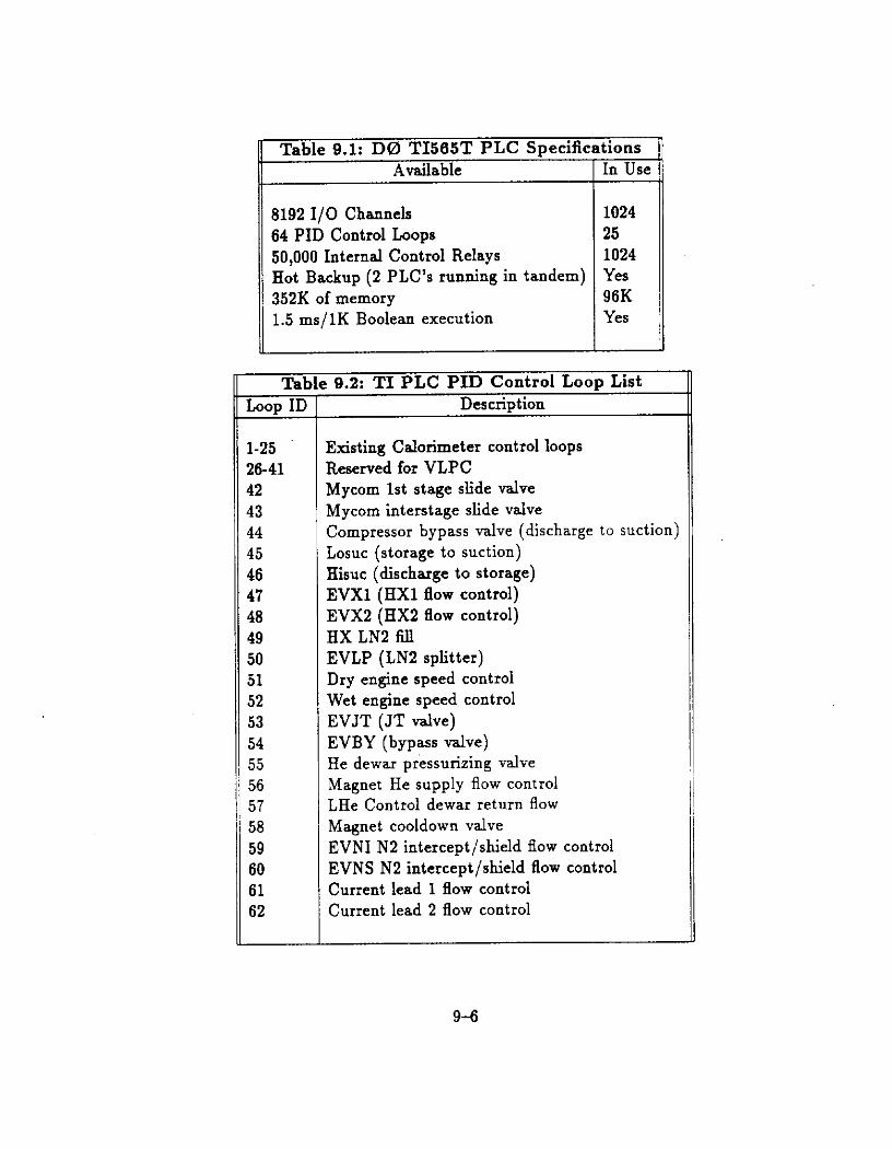
I

I

2

4

4

4

4

4

4

4

1

:

:

! I

I

L

I

I

I

I

I

I

I

8192 I/O Channels 64 PID Control Loops 59,999 Internal Control Relays Hot Backup (2 PLC’s running in tandem) 352K of memory 1.5 ms/lK Boolean execution

Table 9.1: DO TI565T PLC Specifications Available I In Use

1024 25 1024 Yes 96K Yes

Table 9.2: TI PLC PID Control Loop List Description ;oop ID

.-25 !6-41 L2 L3 14 L5 16 17 18 19 i0 il i2 53 54 55 56 7 8 ‘9 ‘0 ‘1 82

Existing Calorimeter control loops Reserved for VLPC Mycom 1st stage slide valve Mycom interstage slide valve Compressor bypass valve (discharge to suction) Losuc (storage to suction) Hisuc (discharge to storage) EVXl (HXl flow control) EVX2 (HX2 flow control) HX LN2 fill EVLP (LN2 splitter) Dry engine speed control Wet engine speed control EVJT (JT valve) EVBY (bypass valve) He dewar pressurizing valve Magnet He supply flow control LHe Control dewar return flow Magnet cooldown valve EVNI N2 intercept/shield flow control EVNS N2 intercept/shield flow control Current lead 1 flow control Current lead 2 flow control

9-6

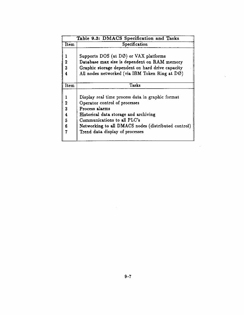
Table 9.3: DMACS Specification and Tasks Item I Snecification

Supports DOS (at D0) or VAX platforms Database max size is dependent on RAM memory Graphic storage dependent on hard drive capacity All nodes networked (via IBM Token Ring at DO)

Item /

I

Tasks

Display real time process data in graphic format Operator control of processes Process alarms Historical data storage and archiving Communication5 to all PLC’s Networking to all DMACS nodes (distributed control) Trend data display of processes

9-7

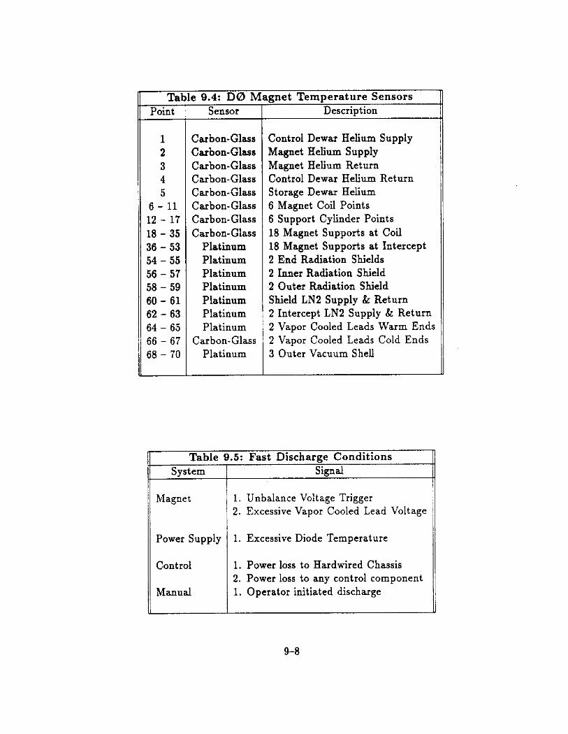
Table 9.4: DO Magnet Temperature Sensors 1 Sensor I Description Point

1 2 3 4 5

6 - 11 12 - 17 18 - 35 36 - 53 54 - 55 56 - 57 58 - 59 60 - 61 62 - 63 64 - 65 66 - 67 68 - 70

L

,

t

,

I

,

Carbon-Glass Control Dewar Helium Supply Carbon-Glass Magnet Helium Supply Carbon-Glass Magnet Helium Return Carbon-Glass Control Dewar Helium Return Carbon-Glass Storage Dewar Helium Carbon-Glass 6 Magnet Coil Points Carbon-Glass 6 Support Cylinder Points Carbon-Glass 18 Magnet Supports at Coil

Platinum 18 Magnet Supports at Intercept Platinum 2 End Radiation Shields Platinum 2 Inner Radiation Shield Platinum ,2 Outer Radiation Shield Platinum Shield LN2 Supply & Return Platinum 2 Intercept LN2 Supply & Return Platinum 2 Vapor Cooled Leads Warm Ends

Carbon-Glass 2 Vapor Cooled Leads Cold Ends Platinum 3 Outer Vacuum Shell

Table 9.5: Fast Discharge Conditions System Signal

I Magnet 1. Unbalance Voltage Trigger

2. Excessive Vapor Cooled Lead Voltage

Power Supply 1. Excessive Diode Temperature

Control

Manual

1. Power loss to Hardwired Chassis 2. Power loss to any control component 1. Operator initiated discharge

9-8

System

Magnet

Power Supply

Cryogenics

Table 9.6: Slow Discharge Conditions Signal

:ontrol

1. Magnet Current high 2. Excessive Ground Fault Current 3. Vapor Cooled Lead Flow Inadequate 4. Cryostat Vacuum Pressure High 5. Lead Guard Vacuum Pressure High 6. Radiation Shield Temperature High

1. Loss of Primary 3@ Power 2. Cover Open in Energization Circuit Enclosures 3. Water Cooled Bus Temperature High 4. Reversing Switch or Filter Choke Temperature Higl 5. Protection Resistor Temperature High

1. Solenoid Cold Mass Temperature high 2. Control Dewar Helium Level Low 3. Helium Supply Temperature High 4. Helium Supply Dewar Low 5. Helium Pressure High in Solenoid 6. Helium Flowrate Low in Solenoid

1. PLC Abnormal 1. UPS battery Low 3. QPM Chassis Abnormal

1. Operator initiated command

9-9

Table 9.7: Interlock Conditions II Pnwer Supply Operation II

Item

1 2 3 4 5 6 7 8 9 10 11 12 12 13

_ -..-_ 1( Buswork covers on and doors closed

Protection resistor temperature low Master chassis key enabled QPM status normal and reset Fast discharge switch closed Operator command “on” Reversing switch key “disabled” UPS status normal PLC’s normal 30 power available to Power Supply Magnet temperature 2 6 Kelvin Magnet Cryostat Vacuum normal Cry0 “summation” normal Warm current bus temp “normal”

Item Reversing Switch Operation

Condition

1 Master Power Supply Key disabled 2 Magnet current minimal 3 Magnet voltage zero 4 Power supply off 5 Power supply voltage zero

9-10

DO CRYOGENIC CONTROL CONFIGURATION

(‘DARKER LINES REPRESENT EXISTING SYSTEM)

“LPC CR”OGEW

SOLENOID CR”OGEWIC!

M m 18 P,O LOOPS 5 PID LOOPS 83 AIWLCG 110 I5ANMoGKl 10 oI(IITN. m 10 OmTATIL I*)

I I

I I “EL,“” REFRIGERAT R HEUUY TEYPER*T”RE 1 DNlCE s*oE 1

* m OPIDUOPS 15PIOLcaFs

Bo*wKem IIWOOLQ 2 DlGmL 10 2oDOITN.Kl

IyI cmEwBLE,.F*5TovMP

2. SLOW DUMP

11

Figure 9.1

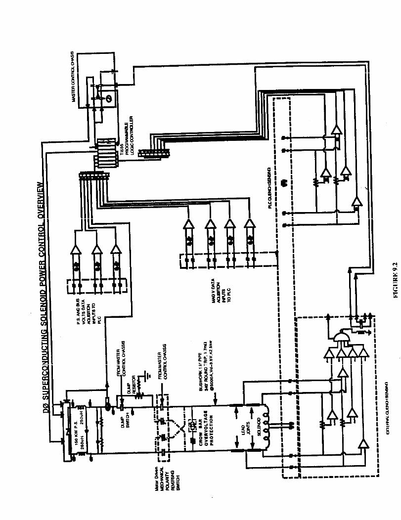
I I I I

L-4 I

m--m_---------d

CHAPTER 10

DC ENERGIZATION CIRCUIT

10.1 DC Current Regulated Power Supply

The PEI 150 power supply [l] to be provided for the solenoid is a special Fermilab unit designed for superconducting loads. The electrical input requirements of the supply are 480V 30, approximately 240A at rated output. The PEI 150 is a twelve phase thyristor water cooled rectifier unit with precision feedback current regulation; it is provided with series/parallel taps for both primary transformer connections and output SCR grouping.

The power supply taps can be set at 30V/5000A or 15V/5000A. It is preferable to set the power supply taps at 15V/5000A because the overall operation is more efficient, the power factor is better, and the ac loading and dc output ripple voltage are reduced. The differences are listed in Table 10.1.

The feedback regulator has an internal current transductor to regulate current to within 0.05%. The power supply is expected to regulate the current to within 0.01% [2]. An internal shunt is used for the panel ammeter mounted on the front of the supply. The internal transductor measures the sum of the filter current and the load current and therefore in order to regulate the load current an external precision Holec 5000 Amp transductor [3] is to be installed downstream of the ripple filter and dump resistor. This device will provide the current feedback signal to the power supply regulator. Internal status of the power supply is monitored and a summation of its internal interlock string is necessary for turn-on. External permits and interlocks also can be introduced into this summation via an available connector. The power supply is programmable. It can be turned on and off remotely when the interlocks are ready and reset. A precision external reference is used to set the current. A rate control chassis [4] wiU be installed to limit the rate of current change to the desired value (see Chapter 11) during magnet energization. The rate control chassis must be installed in the power supply at the power supply regulator output. Installing current rate control at the sensitive reference input location will deteriorate power supply current regulation.

The output power circuit of the supply contains freewheeling diodes. These diodes con- duct the current decay when the supply is turned off. Because the power supply and filter chokes are not rated to carry the decaying current during a cooling water failure, an extra set of freewheeling diodes sized for a slow discharge from full current without cooling water is therefore added behind the filter. These diodes also prevent polarity reversal at the filter capacitors.

The grounded steel enclosure with interlocked doors and a lockable main power circuit breaker are safety features. A lighted front panel provides operating status.

10-l

10.2 Ripple Filter

In order to prevent external electrical noise from being transmitted into the quiet environment of the detector a filter [5] wilI be installed on the output of the power supply. Each polarity will connect to a 5000 A, 230pH choke [6]. Th e chokes provide high current capability with low loss in a small package. They are constructed with split laminated cores and use an economical method of construction for air gap reactors.

The shunt capacitance needed is in the range of 9000 to 45000 pF. Further circuit analysis and simulation will be required to finalize the actual component choices and the extent of overvoltage protection required by the capacitors. The electrolytic capacitors are protected from reverse voltages during magnet discharge by the freewheeling diodes. The capacitors are not expected to require an active SCR crowbar circuit to clip surges that would exceed the& specifications [5]. The filter capacitor must have a minimum operating working voltage of 250Vdc, and a surge voltage rating of 325Vdc. The filter must be able to withstand 1250Vdc test to ground.

10.3 Dump Switch and Protection Resistor

A 5000Adc/lOOOV contactor, such as Siemens Allis type 703 [7], is provided as a dump switch. A similar Allis type 703 switch is installed in the proton beamline at PE3Q2. A solid state switch [8] could also be used; such a switch is highly reliable but at 5000A would create about 3kW losses. Because the solenoid is designed to quench without damage without a protection resistor, a backup to to the dump switch will not be installed.

The air-cooled protection resistor will be fabricated of stainless steel bars weighing 120 kg welded in series and installed in a metal enclosure [9]. Th e resistor provides a resistance of 48 x 10-s Ohm at 20% to limit the fast discharge voltage to 250V maximum; its temperature rises to 1OO’C during a discharge of 5MJ. The midpoint of the protection resistor is connected to ground so that the maximum coil voltage to ground does not exceed 125V peak during a discharge from 5000A. The resistor will retool in about 30 minutes following a fast discharge.

A trigger fuse or resistor on the grounded center tap of the protection resistor will limit unexpected ground fault currents to less than 40A. X ground fault detection chassis will be provided for the center tap.

The protection resistor is connected in parallel with the dump switch so that the 5OOOA dc circuit is never fully interrupted. This arrangement allows the stored energy in the power supply and the filter chokes to escape via the protection resistor. A capacitor of about lOOOpF, 500V is installed across the dump switch to suppress spikes.

10-2

10.4 Reversing Switch

Reversal of the load polarity will be accomplished with an available 5000A dc mechanical, motorized polarity reversing switch [lo] and a switch controller. Polarity reversal requires a slow discharge and recharging of the solenoid. Initiating a fast discharge below the point where the decaying current can no longer cause a quench can speed the discharge. Reversing is expected to take approximately 40 minutes. The switch is presently in storage at Fermilab and will be refurbished for its new installation. It measures approximately 4 feet per side, is floor mounted and requires no water cooling. The controller performs the critical functions which assure that the polarity reversal occurs at zero load current and that the power supply is turned off. Some modification to the operation of the existing mechanical timer system in the controller wilI be required to interface with the DO PLC system. A set of maintained closed (forward) contacts or maintained open (reversed) contacts can be monitored and selected by the PLC. Changing the status of the contacts begins a timing sequence in the controller which powers the supply off to initiate a slow discharge of the magnet. The built in timing control of the controller reverses the switch after a preset delay and releases the power supply rate control chassis. The reversing switch timing control uses a motor driven timer with cam switches and is not affected by power interruptions. Once it is started it must complete a sequence before it can be used again.

10.5 Crowbar

An overvoltage protection crowbar [5] will b e installed in parallel with the solenoid between it and the reversing switch. This crowbar serves as a safety backup for the interlocks on the reversing switch so that in the event of equipment failure, the operation of the reversing switch under load does not cause destructively high voltages. The crowbar will be set to trip and limit the maximum solenoid voltage to 300V peak, above the normal fast discharge voltage of 250V peak. The crowbar consists of several back to back SCR’s in parallel. Each back to back set of SCR’s has a series resistor to assure current sharing and at the same time dissipate the stored energy of the solenoid. The combined weight of aJl the series resistors is about 250 lbs. The crowbar is completely self-contained and does not require any auxiliary power to trip. The crowbar SCR voltage rating should be chosen at 500 V. The SCR’s will break down if the crowbar firing fails. This provides two levels of protection: 300 V and 500 V.

10.6 Water Cooled Bus

A 5000A dc copper bus system is provided to connect the power supply system to the superconducting load. The one-way distance from the power supply area to the Assembly Hall Detector location is approximately 21 meters and an additional 23 meters to the location

10-3

in the Collision Hall. A standard bus construction, widely used in the Fermilab Experimental Area will be used 111). It consists of supply and return conductors of high conductivity, 3.8 cm square “double extra strong” copper pipe. A high impact PVC (or equivalent) insulating pipe is slipped over the copper pipe for electric insulation. The copper pipes are joined by brazing or silver soldering with straight couplings or elbows ss required. The joints are then insulated with shrink-on sleeves. Copper flags are brazed to the ends of the bus for cable attachment. A suspension system of Unistrut and pipe clamps will be required to route the bus. One set of flags taps off the bus at the Assembly Hall location for the detector and another in the Collision Hall. Water cooling is accomplished with LCW hose connections to the bus end caps. Overtemperature switches are installed near the cable connection flags and these are wired to the interlock system. The watercooled bus can dissipate all stored energy if a fast discharge is triggered by a cooling water failure which then fails over to a slow discharge due to failure of the dump switch. The maximum expected temperature of the buses in this instance is 91°C. From experience with similar installations this bus is simple to install, is rugged in service, and meets aU safety requirements.

To equalize test conditions in the Assembly Hall and the operation conditions in the Collision Hall a small length of stainless steel watercooled pipe may be added to the buswork in the Assembly Hall to make the Assembly Hall bus resistance the same as the Collision Hall bus resistance (see table 10.1).

10.7 Quench Detection

Quench detection will be accomplished by providing redundant balanced bridge circuits and voltage taps on the coil, superconducting buses, and vapor cooled leads. As described in Chapter 9, four coil taps are provided on the coil: one each at the start and finish of the coil winding and two additional taps, one near the center and another near the 3/4 point as diagrammed in Figure 10.2. Each bridge must be balanced for zero output during solenoid initial startup to enable the lowest practical threshold levels to be selected thereafter while preventing nuisance trips. The quench detector bridges can use iso-op amp style isolation as shown in Figure 10.2 or a magnetically coupled technique !12] which is presently under development. Both isolation methods are similar but the magnetically coupled type is expected to provide better noise immunity and better personnel safety.

A redundant set of quench detectors is provided. The first set will be monitored by a hardwired QPM chassis and the redundant set will be routed to the PLC for software quench detection. The QPM will provide the first line of defense for quench detection by means of lower threshold reference values. Quench threshold levels will be established during preliminary low-current charging exercises prior to full current operation of the magnet. The quench detectors are fail-safe and must be connected otherwise they will cause an interlock trip.

10-4

10.8 Interlocks and Controls

A possible interlock and control flow diagram for the magnet energization system is shown in Fig. 10.3. The diagram shows many interlocks and others may have to be added as the design is finalized. Additiona detail on the interlock system is provided in Chapter 9. Ail controls wiII be via the PLC as described in Chapter 9. Status monitoring (voltage taps, etc.) from the solenoid must be via a different set of safety isolation resistors and monitoring cables as described in Chapter 9.

References

[l] PEI 150 Model SR-1029, NAL Spec 6065-ES-44047; Engineered Magnetics, Inc 18435 Susanna Road, Ranch0 Dominguez, CA 90221

[2] A.T. Visser, “Magnet Power Supply Regulation Comments 240 kW and 500 kW Magnet Power Supplies”, Fermilab TM 1890, March 1993

[3] Holec, Inc. 12502 Exchange Dr., Suite 404, Stafford, TX 77477

141 See e.g. Fermilab EED Drawing 6005-ED-172973

[5] E. Drennan, “Ripple Filter for the 10,000 A Superconducting Magnet Test Stand at the Magnet Test Facility”, FERMILAB-TM-1764, Nov 1991.

[6] A. T. Visser, “Electrical Design Note for a 5000 ADC, 230 PH Power Supply Filter Choke”, FERMILAB-TM-1836, Apr 1993,

[7] Siemens Energy & Automation, Inc., PO Box 8900, Atlanta, GA 30356.

[8] A. T. Visser, “Design Note of a 10,000 A, 1000 V Solid State Dump Switch for the Magnet Test Facility”, FERMILAB-TM-1692, Ott 1990.

]9] A. T. Visser, “Design Note of a 10,000 A 2 MJouie Dump Resistor for the Magnet Test Facility”, FERMILAB-TM-1611, Mar 1990.

[lo] GouId/ITE Model SO 45-03951, Fermilab Spec 2816-38-38314; Gould Shawmut, 374 Merrimac St., Newburyport, MA 01950.

[ll] A. T. Visser, “Description of a High Current Water Cooled Bus”, FERMILAB-TM- 1372, Dee 1985.

[12] A. T. Visser, et. al., “A Magnetically Coupled Quench Detector for Superconducting Magnets”, Fermilab TM 1870, Oct. 1993.

10-5

Table 10.1: Electrical System Parameters Parameter PS Tap 30 V, 5000 A PS Tap 15 V, 5001

YominaI Operating Current 5000 A Same

Maximum Allowable dI/dt 1720 A/tin Same Maximum Dump Voltage 250 V Same

Maximum Insulation Test Voltage to ground (1 min) 1250 V DC Same

Magnet Stored Energy 5.6 MJ Same

Circuit Inductance 0.53 H Same

Circuit Resistance (CH) 2.3 x 1O-3 Same

Circuit Resistance (AH) 1.5 x 10-s Same

CH(AH) Slow Dump Time Constant 230 (353) seconds Sane CH(AH) Fast Dump Time Constant 10.5 (10.7)seconds Same

Charging Time 7 minutes Same :H(AH) Slow Dump Time 20 (25) minutes Same

Fast Dump Time 50 seconds Same DC Current Reversing Time 37 minutes Same

Power Supply Max Voltage 34 17

Current Regulation 5 100 ppm at > 1000 Adc Same External Reference 5 5 ppm/“C, 2 16 bit Same

O-10 V dc, 500 A/v Same

CH(AH)Operating DC Voltage z 8 (12)V Same

Output Ripple P to P zz 5.6 V z 2.2 v

AC Input 480 V, 30, 240 A,60 Hz Same Except 120 Input Power Factor 0.3 (0.2) 0.6 (0.4)

Ripple Filter Chokes 2 x 230/.~H Same 2 x 0.38 x 10-s Same

CH (AH) Bus 5000 A, 3.8 cm nom. Cu pipe i Same 1.5 x 10-s (0.7 x 10-3) Same

91 (43) m Same

Protection Resistor 48 x 1O-3 Same

120 kg AT x 100°C at 5.6 MJ

Dump Switch 5000 A Contactor Same

10-6

Table 10.1: Electrical System Parameters, cont. Parameter 1 PS Tap 30 V, 5000 A 1 PS Tap 15 V, 5000 A

1 I

II Reversinn Switch 5000 A Mechanical Same II Overvoltage Crowbar 300 V, 5000 A peak Same

Cooling Water Same

Resistivity 13 MRcm, LCW Power Supply 19 I/s, AP = 690 kPa Chokes Each 4 l/s, AP = 690 kPa Bus at 40°C Rise 15 (8) l/s

Over Temperature Protection 80°C Same

Losses 69 kW Total Same

Power Supply 12 kW Same Chokes 19 kW Same Bus 38 (18) kW Same

10-7

-, 3 - ‘- i

++-c2 -

n -- l

__----- --

s

t a-

!E 2% :N CE

-> $

J2 Q$ ?P _- ;g

3g .

-----A---

..-,

f < 2 ; 2 .1 zj ;i 2 = -

-2 s;,, ,..? = 5 - F <Q - e 3 3 Z’n;?” ; y:,- 5_ = : 5 E 5

.7 6 &i- .=-

5 z:d T - 3 2 3 c g

f-9 ---------

‘

7 z-

3 - g ’ m

c i=z= ::

03Yti E ;

5 ;;g;: z E -- - -G 2 c z - -----. L

r.

e 0 ,z i 0 5 L 2 z .” E 2 z k b

-

:_I ~5 ui

;R 2 ui =

:I 2 5% til s +t t =i -

A

gi

g; 81,

F7 u1 > 4

k = E z x

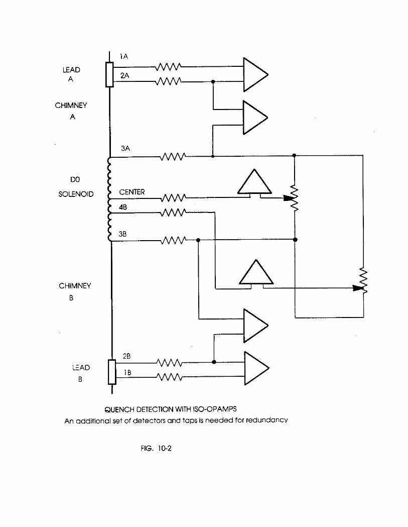
LEAD A

CHIMNEY

A

DO

SOLENOID

CHIMNEY

B

LEAD

B

1A

3A

1

CENTER A i . . . .

48 I. *.

28

1B

QUENCH DETECTION WITH ISO-OPAMPS

An additional set of detectors and taps is needed for redundancy

FIG. lo-2

i &IIII ----- 1-2

--------

i 5

% i 2

‘I:

z d 1%

:j z =” y,. :3 S” J-

$ i 1

; 21

: ;I I

si.ii I

!

gg&gg/ .$ A jf~fhdtj”fp&i srrxPP?siZan-

CHAPTER 11

QUENCH CALCULATIONS

11.1 Quench Codes

The quenching of the magnet has been modeled using a version of the program QUENCH created by M.N. Wilson [l]. Program QUENCH simulates the quenching of a superconducting magnet by propagating an ellipsoidal normal zone throughout the volume of the quenching coil. It calculates the ohmic heating and adiabatic temperature rise of the coil while the current decays as the stored energy of the magnet is dissipated. From a given starting point the normal zone volume is expanded by three orthogonal quench velocities in finite time steps. The quench velocity in the longitudinal direction of the conductor is calculated from the thermal and critical properties of the superconductor, the operating temperature of the magnet, and the current density in the coil. The velocities in the orthogonal directions are scaled from the longitudinal velocity by the one half power of the ratios of the thermal conductivities in the windings. The temperature dependent properties of each material making up the coil is provided, as is the total volume of the coil (expressed as an equivalent parallelopiped), and the resistive characteristics of the external circuit. QUENCH conveniently notes the time at which the current has decreased to l/e of its original value, and the time at which the entire volume of the coil has become normal. Because QUENCH assumes adiabatic conditions the peak temperature of the coil occurs at the point where the quench was started. It is conservative to specify the starting point of a quench at one (physically meaningful) edge of the coil parallelopiped to obtain the least amount of coil driven normal per unit time during the quench.

11.2 Quench Study

QUENCH was modified [2] to allow the specification of more than one current density in the windings so that the winding design of the D0 magnet could be accommodated. In Figure 11.1 is seen the results of the calculations for the magnet, quenching into a 50 milliohm protection resistor. An RRR of 500 was used for the aluminum stabilizer, and the presence of the outer support cylinder was ignored. The quench was initiated at one end of the coil winding. The aggregate time constant of the decay is 11 seconds (L/R for the system prior to the quench is 0.48/0.050 = 9.6 seconds), the maximum temperature of the coil is 58 K and the coil resistance rises to 51 milliohms.

The spreading of the normal zone from the starting point is schematized in Figure 11.2. The resistivities of the aluminum and copper in the coil are shown in Figure 11.3. The

11-l

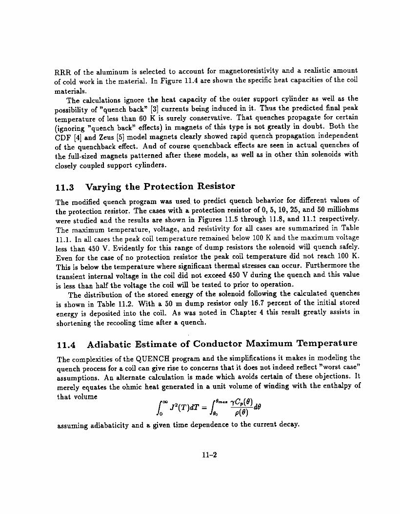
RRR of the aluminum is selected to account for magnetoresistivity and a realistic amount of cold work in the material. In Figure 11.4 are shown the specific heat capacities of the coil materials.

The calculations ignore the heat capacity of the outer support cylinder as well as the possibility of “quench back” [3] currents being induced in it. Thus the predicted final peak temperature of less than 60 K is surely conservative. That quenches propagate for certain (ignoring “quench back” effects) in magnets of this type is not greatly in doubt. Both the CDF [4] and Zeus [5] model magnets clearly showed rapid quench propagation independent of the quenchback effect. And of course quenchback effects are seen in actual quenches of the full-sized magnets patterned after these models, as well as in other thin solenoids with closely coupled support cylinders.

11.3 Varying the Protection Resistor

The modified quench program was used, to predict quench behavior for different values of the protection resistor. The cases with a protection resistor of 0, 5, 10, 25, and 50 milliohms were studied and the results are shown in Figures 11.5 through 11.8, and 11.1 respectively. The maximum temperature, voltage, and resistivity for all cases are summarized in Table 11.1. In all cases the peak coil temperature remained below 100 K and the maximum voltage less than 450 V. Evidently for this range of dump resistors the solenoid wilI quench safely. Even for the case of no protection resistor the peak coil temperature did not reach 100 K. This is below the temperature where significant thermal stresses can occur. Furthermore the transient internal voltage in the coil did not exceed 450 V during the quench and this value is less than half the voltage the coil will be tested to prior to operation.

The distribution of the stored energy of the solenoid following the calculated quenches is shown in Table 11.2. With a 50 m dump resistor only 16.7 percent of the initial stored energy is deposited into the coil. As was noted in Chapter 4 this result greatly assists in shortening the retooling time after a quench.

11.4 Adiabatic Estimate of Conductor Maximum Temperature

The complexities of the QUENCH program and the simplifications it makes in modeling the quench process for a coil can give rise to concerns that it does not indeed reflect “worst case” assumptions. An alternate calculation is made which avoids certain of these objections. It merely equates the ohmic heat generated in a unit volume of winding with the enthalpy of that volume

/,- JZ(T)d’f = /,“-” ‘gd@

assuming adiabaticity and a given time dependence to the current decay.

11-2

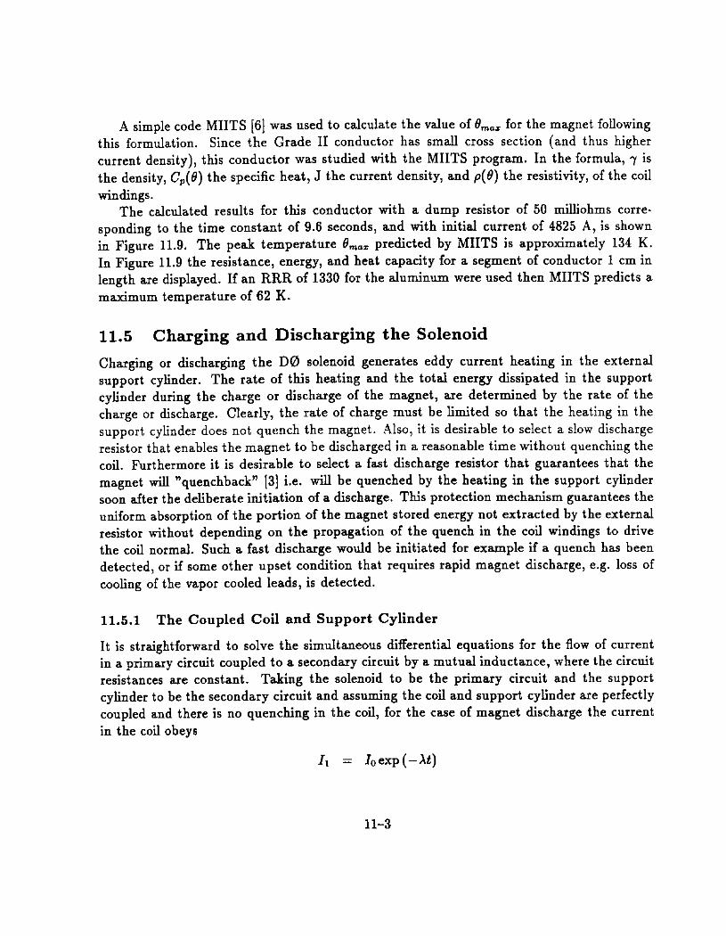
A simple code MIITS [6] was used to calculate the value of 6’,,, for the magnet following this formulation. Since the Grade II conductor has small cross section (and thus higher current density), this conductor was studied with the MIITS program. In the formula, -y is the density, C,(B) the specific heat, .I the current density, and p(B) the resistivity, of the coil windings.

The calculated results for this conductor with a dump resistor of 50 milliohms corresponding to the time constant of 9.6 seconds, and with initial current of 4825 A, is shown in Figure 11.9. The peak temperature B,., predicted by MIITS is approximately 134 K. In Figure 11.9 the resistance, energy, and heat capacity for a segment of conductor 1 cm in length are displayed. If an RRR of 1330 for the aluminum were used then MIITS predicts a maximum temperature of 62 K.

11.5 Charging and Discharging the Solenoid

Charging or discharging the DO solenoid generates eddy current heating in the external support cylinder. The rate of this heating and the total energy dissipated in the support cylinder during the charge or discharge of the magnet, are determined by the rate of the charge or discharge. Clearly, the rate of charge must be limited so that the heating in the support cylinder does not quench the magnet. Also, it is desirable to select a slow discharge resistor that enables the magnet to be discharged in a reasonable time without quenching the coil. Furthermore it is desirable to select a fast discharge resistor that guarantees that the magnet will “quenchback” [3] i.e. will be quenched by the heating in the support cylinder soon after the deliberate initiation of a discharge. This protection mechanism guarantees the uniform absorption of the portion of the magnet stored energy not extracted by the external resistor without depending on the propagation of the quench in the coil windings to drive the coil normal. Such a fast discharge would be initiated for example if a quench has been detected, or if some other upset condition that requires rapid magnet discharge, e.g. loss of cooling of the vapor cooled leads, is detected.

11.5.1 The Coupled Coil and Support Cylinder

It is straightforward to solve the simultaneous differential equations for the flow of current in a primary circuit coupled to a secondary circuit by a mutual inductance, where the circuit resistances are constant. Taking the solenoid to be the primary circuit and the support cylinder to be the secondary circuit and assuming the coil and support cylinder are perfectly coupled and there is no quenching in the coil, for the case of magnet discharge the current in the coil obeys

11 = loexp(-Xt)

11-3

where Z. is the current in the magnet before the discharge, and

X = (RI&)/(&& + Mh)

= l/(71 + rr).

The current in the support cylinder obeys

MAZ, I2 = Zz(X* -A) [exp (-At) - exp (-&t)] .

with Z, the inductance of the coil, RI resistance of the protection resistor, and Zr and Rz the inductance and resistance of the support cylinder, respectively. X; = Zi/& and M =

Gz. The instantaneous power developed in the support cylinder by this current is just P(t) =

ZiR2. The total energy dissipated in the support cylinder is just the integral of the power during the discharge, and since Er = (1/2)ZrZi, this can be written

E1RzZJ2 Ez = L;(& -X)2 x

For the values of the parameters which pertain to the DO magnet X1 <( Xs, and Z,/Zr = N2 where N is the number of turns in the solenoid so that

RI Ez N El----. RzN2

This heating must be compared to the available cooling of the support cylinder and the thermal margin defined by the critical properties of the superconductor.

11.5.2 Cooling the Solenoid

As was shown in Chapter 4, ANSYS modeling of the cooling tube and coil support geometry on the coil support cylinder indicates that the maximum conductor temperature expected during steady-state operation of the magnet is about 4.9 K. The temperature of the helium in the cooling tubing is fixed at 4.7 K as predicted by the flow calculations for the cooling tube system. This 0.2 K temperature elevation of the conductor above the temperature of the cooling tubes is caused by heat conduction to the support cylinder from the support members and radiation from the shield.

Uniform additional steady heat generation can be added to the support cylinder in the ANSYS model and the added elevation of the conductor temperature due to this heating obtained from ANSYS.

In Figure 11.10 is seen the correlation predicted by ANSYS for additional heating in the support cylinder and the conductor temperature elevation caused by it. For e.g. 45 Watts added steady heating in the support cylinder it is seen that the conductor temperature is expected to be elevated about 0.4 Kelvins, to an operating temperature of about 5.3K.

11-4

11.5.3 Charging the Solenoid

For the case of a uniform charging voltage El on the superconducting coil, the coupled equations yield the solutions

z, = MG x2zlz2 bd-W - 11

The power dissipated in the support cylinder during such a chargeup is just Z’(t) = Z(t)iR2. For the values of the parameters pertaining to the DO magnet, the term in square brackets approaches minus 1 almost immediately and we have

P N 0.306 x E;.

For a steady heating power of e.g. 45 Watts, the charging voltage is 12.1 Volts. For a choice of critical parameters of the superconductor such that the operating current

is 50% of the critical current at the nominal operating temperature, the current sharing temperature of the superconductor is approximately 6.8 K, about 1.9 K above the nominal operating temperature of the conductor. Even with this specification and Figure 11.10, it remains judgmental to choose a safe charging voltage. Given the potential for variability in the quality of the conductor and the operational stability of the cryogenic system a charging voltage of 6 V is selected (with perhaps an even lower voltage when near the final operating current). The actual voltage selected may also be reduced during the initial charge-up depending on the frequency and amplitude of any conductor motion perturbations observed.

For a fixed 6V charging rate the full operating current of the magnet is reached in about six minutes. As was shown in Chapter 10 the power supply will have to provide approximately an additional 8 V at full current for the bus resistance to the collision hall.

11.5.4 Discharging the Solenoid

A slow discharge that is conveniently rapid but yet does not cause the magnet to quench is desired for normal turn-off of the magnet. Quenches will cause a measure of upset to the cryogenic system and require re-cooling of the magnet before it can be repowered. Avoiding these complications during normal discharge of the magnet is desirable.

As indicated above it should be conservative to discharge the magnet from full current with 45 Watts initial eddy current heating in the bore tube.

From the discharging equation for 12 above the instantaneous power dissipated in the support cylinder during a magnet discharge can be evaluated. For the range of values of the discharge resistor R, between 0.0015 and 0.09 Ohms this power peaks rapidly in about one second or less after the initiation of the discharge then decays slowly thereafter according to

11-5

the time constant ZI/R1 of the primary circuit. In Figure 11.11 is seen this peak power as a function of the value of the discharge circuit resistance. Evidently we can choose the slow discharge resistance to be 0.0025 Ohms or less (corresponding to a peak power of about 45 Watts or less) and be assured that the magnet will not quench.

With a slow discharge resistance of 0.0025 Ohms the magnet is discharged to less than 10 amperes in about 20 minutes.

We can ignore the cooling power provided by the cryogenic system during a discharge and using the discharge equations calculate the total energy dissipated in the support cylinder for various values of the resistor RI. Using the enthalpy of the aluminum in the support cylinder mass, we calculate the final temperature of the support cylinder due to the energy deposited in it (Figure 11.12). Evidently for even the most rapid discharges the support cylinder temperatures do not approach temperatures where thermal stresses need be considered.

Quench calculations have been made which indicate that for reasonable modeling of the quench velocities in the coil windings the magnet will quench safely. To avoid risk due to the uncertain nature of these cabculations a fast discharge resistance can be specified that is certain to cause a rapid quench via the quenchback effect. A fast discharge is in fact desirable to ensure the safety of the vapor cooled leads and buswork in the chimney in the event upsets are detected in these components as detailed in Chapters 9 and 10.

In Figures 11.13a and 11.13b are shown the time after the beginning of the discharge at which the support cylinder has reached 9.2 Kelvins assuming no heat removal from the support cylinder during this exercise, as a function of the time constant of the decay. (Figure 11.13b is a restricted portion of 11.13a. The discretized time values in the expanded-scale plot of Figure 11.13b are caused by the finite time steps selected by the program which calculates the support cylinder warmup).

From Figure 11.13 we specify that a fast discharge resistor 2 0.04 Ohms be provided to ensure that the coil will be protected by the quench back effect.

In Figure 11.14 we show the total time for discharging the magnet to less than 10 amperes as a function of the choice of discharge resistor. For the fast discharge resistor selected, the magnet is discharged in slightly less than 2 minutes.

11.5.5 Fast Discharge Quench Threshold

For a choice of fast discharge resistor of 0.050 Ohms a discharge from 5000 Amperes is certain to cause a quench from the quenchback effect. The very high heating rate in the support cylinder causes its temperature to rise beyond the critical temperature of the superconductor within a half second or so.

It is instructive to estimate what the current threshold is below which a fast discharge is not expected to cause a quench. For the conductor specified in Section 2.2 the current sharing temperature of the superconductor at fulI field is approximately 1.5 K above the operating temperature of the magnet. From the steady-state heating curve in Figure 11.10,

11-6

extrapolated to a T of 1.5 K, it is seen that the corresponding heating rate is about 180 Watts. From the expression for the power dissipated in the support cylinder during a discharge, the peak power is

p=!$ 2

An initial current of 485 amperes will therefore result in a peak discharge power of 180 Watts. (The 5083 aluminum support cylinder has a resistance of approximately 3.2 x 10-e Ohms, not strongly temperature dependent below N 100 K).

This result underestimates the actual quenchback threshold current expected since for a current of 485 Amperes the current sharing temperature is substantially more than 1.5 K above the operating temperature - almost 3.6 K in fact; also, the quenchback power derived is the peak power during the discharge, not the steady-state power required by Figure 11.10.

By integrating the quenchback power throughout the discharge and equating it to the enthalpy of the support cylinder plus one layer of the coil nearest the support cylinder it is seen that for initial currents below about 1770 Amperes the temperature of this portion of the cold mass never reaches the current sharing temperature of the conductor; just above this threshold current the current sharing temperature is not reached until 10 seconds of the discharge have elapsed.

The degree to which this last estimate for the quenchback threshold is conservative or not depends on what effect ignoring the cooling power of the cooling system during the discharge has. For an initial current of 1800 amperes the peak power in the support cylinder is about 2000 Watts. It is not easy to estimate the instantaneous cooling power available from the cooling system, but its steady-state cooling capability is much less than this. It is likely then that ignoring the cooling during the discharge does not constitute a large effect and that the quenchback threshold for the conductor specified is not far fIom 1800 amperes.

It may be desirable during normal slow discharges to in fact trigger a fast discharge when the magnet current has fallen below this level to safely hasten the slow discharge.

11.6 Protecting the Magnet Buses

The vapor cooled current leads in the magnet control dewar are connected to the magnet by superconducting buses nearly 14 meters long. Each bus is made of a parallel pair of magnet conductors thermally anchored to the helium supply tube in the magnet chimney but electrically isolated from it. After the magnet has been cooled to operating temperature and proper vapor flow is established in the vapor cooled leads, the buses in the chimney become superconducting permitting charge-up of the magnet. Subsequent upsets to the cooling in the chimney must enable magnet power-down without the loss of integrity of these buses.

11-7

To determine the operating margins of one of the superconducting buses after it has left the superconducting state we conservatively assume that it is not cooled by the helium supply tube so that ohmic heating in it by the magnet current contributes directly to the temperature rise in it. A discharge resistance ( or equivalently a decay time constant) for the magnet is selected and the magnet current is allowed to decay accordingly. The peak voltage drop on the bus during the discharge is calculated, as is the final temperature at the end of the discharge.

Note that ignoring heat conduction along the bus the final temperature calculated is independent of the length of the segment of the bus that has gone normal. The peak voltage drop calculated however assumes that the entire length of the bus, 13.7 meters, has gone normal.

In Table 11.3 are presented the final temperature and peak voltage drop of the bus where the bus consists of one, two, or three of the magnet conductors in parallel, for several choices of discharge resistor. (Composing the bus of multiple magnet conductors is for convenience; the total amount of low-resistivity aluminum in the bus is what is at issue). The onset of the decay is chosen to begin after the voltage drop of 0.025 V is reached.

The final temperature and peak voltage drop are omitted from the table if the temperature exceeded 600K before the discharge was completed. In general the table shows that it is helpful to add extra normal conductors to the buses to protect them from overheating in the event of an upset. For the faster discharges even the single-conductor bus is safe, and the addition of one extra conductor gives all the protection of three or more conductors for all but the slowest discharges.

The peak voltage drop is typically small but adequate for triggering the magnet discharge reliably. The time elapsed before the desired voltage drop is reached is indicated; it is noteworthy that it depends only on the size of the bus (and the choice of voltage drop before triggering the discharge).

If instead of 0.025 V, 0.050 V is chosen for the voltage drop necessary to trigger the discharge the above table is slightly modified: the final temperatures rise a few degrees, and the peak voltage drops (for all but the slowest discharge and the single conductor bus) clamp at 0.050 V rather than the 0.025 V shown in the table. Also, the delays become 2.6 seconds for the single-conductor bus, 19.5 seconds for the double-conductor bus, and 57.1 seconds for the triple-conductor bus. Evidently, the threshold selected for the triggering of the discharge needn’t be set unreasonably low and the voltage drop on the bus will tend to clamp at the threshold value selected. The temperature rise in the bus is very much faster than the voltage drop - the conductor reaches the transition temperature for NbTi in typically less than one second or so.

In Figure 11.1 is shown the calculated temperature rise and voltage drop for a discharge of the magnet into a 0.050 Ohm protection resistor. It is assumed that any incident that could drive any portion of the bus leads normal would rapidly lead to the entire length of the bus being driven normal. If this were not the case the voltage drops measured would be

11-8

correspondingly smaller. It is not easy to specify what type of incident could lead to upset in the magnet bus

leads. Loss of helium flow in the chimney is the only credible upset mode that comes to mind, triggered by loss of pressure in the supply dewar or by misoperation of the JT valve in the subcooler circuit. In any case, flow meters will signal this upset and within a few seconds trigger a fast discharge of the magnet. A calculation shows that there is sufficient liquid helium in the chimney pipe above the buses such that 2 minutes elapse after flow stops before the heat load in the chimney generates enough vapor to displace the liquid down to the level of the buses themselves.

References

[l] M.N. Wilson, “Computer Simulation of the Quenching of a Superconducting Magnet,” RHEL/M151, 1968.

[2] A. Mesin and R. Yamada, “Quench Program DDESQUENCH (Modified QT.CNTL)“, D0 Note 1138, May 31, 1991. QT.CNTL is a version of the Wilson code installed at Brookhaven National Laboratory by A.D. McInturff (BNL 19883, 1975) and at FermiIab by A.D.McInturff, and subsequently modified by M. Wake, T. Tominaka, and M. Takasaki (1982).

[3] M.A. Green, “Large Superconducting Detector Magnets With Ultra Thin Coils For Use in High Energy Accelerators and Storage Rings”, LBL-6717, Aug 1977, and Proceedings of the 6th Int. Conf. on Magnet Technology, Bratislava, 1977.

[4] S. Mori, et. al., “Construction and Testing of Superconducting Solenoid Magnet Model for Colliding Beam Detector”, Advances in Cryogenic Engineering 27, Plenum, 1981, p151.

[5] A. Bonito-OIiva, et.aL, “Quench Behaviour of a Thin Solenoid Model”, Proceedings of the llth International Conference on Magnet Technology, Tsukuba, Japan, 1989, p229.

[6] R. Yamada and A. Mesin, “Estimated Maximum Temperature of Conductors for 2 Tesla DO Superconducting Solenoid in Adiabatic Condition”, DO Note 1975, Nov. 12, 1993. MIITS was developed from program HOTCM created by M. Kuchnir, Fermilab. See also R. Yamada, dal., “Estimated Maximum Temperature of Conductor of Superconducting Solenoid Coil in Adiabatic Condition (I)“, KEK Internal 81-10, January, 1982, TRISTAN.

11-9

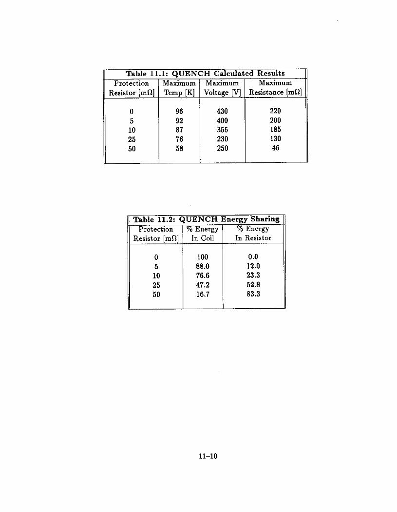
Table 11.1: QUENCH Calculated Results n .

I

Igble 11.2: Protection

Resistor [ma]

0 5 10 25 50

Maximum Maximum Voltage [V] Resistance lmnl

430 220 400 200 355 185 230 130 250 46

JENCH Energy Sharing G Energy % Energy In Coil

f

In Resistor

100 88.0 76.6 47.2 16.7

0.0 12.0 23.3 52.8 83.3

11-10

Protection Resistor [a]

0.0500

0.0309

0.0120

0.0072

0.0025

Delav

One knit :0.735ny

37 K (0.33 V)

49 K (0.046 V)

296K (5.1 V)

tttt*t ******

****** ******

1.1 Set

[1.47n2]

31 K (0.025 V)

33 K (0.025 V)

44 K (0.036 V)

64 K (0.11 V)

****** ******

10.7 Set

l’hree Ifnits [2.21f.d]

33 K (0.025 V)

34 K (0.025 V)

39 K (0.025V)

44 K (0.028 V)

112K (0.44 V)

34.8 Set

11-11

4m.m

xD.0

ma.1

Irn.

a.m-

2.m

0 .

(+)

w.o(

MI

CL,

N

1.

0.

x>

m

0.

W ,,,a I.mO. w-d w

ccm

nm

m

>m

\,

\

\

,. ,-

0.

0

(.I - VA

/

‘l +4 ‘.. $4 4 +“.

$ ...

\\ ++

f r’

6 i

\

IL!. th (-4

““T

HR

- a.

FIG 11.1: Quench with Dump Resistor = 50 rnOhm

E E u-l

0 K 5: Pi 2 v- .- cn’j E CC 2 a 0*c 3Y U>r. CL a0 OU NCU .-

on t

EC LO:

:i- VI,

z- 0

-0 c” al (IO@

.o - .o

cc (yU.-

b 0.F i’

+ u-i I 0

7

-k

II

f- j

d I 0

*

,*)O

NO

-0

OO

(w3*suJyo) AJ!A!gs!say

L K a 6 -0 c 0

E 3 c .- E

s

“0 x + .- > .- -w 0) .- t K

0 i 0 0 0 0 0 0 0

(m/r) awn(oA ~!un Aad Xjpodo3 1~3~

In 0 ‘L al +- 2 I z IL

r” +J ;j

! 0 > ” :

b a x .+i : : 0 4J : I

G 2

-_ I-

u I_.

Pm IP

.m. .-.

u a-

. --

c .-

* I

I. . I

Y1

7,

R

“0 ,,J: Ovench with Dump Resislor = 0 mOhm

RGtt.6: Quench with Dump Resistor = 5 mOhm

( ,--., .a-, -v-7-------

--IllhI L---+-AI” -I 11.1 --

-. .“d. --

mm 9-a --

e. .m* -

I * *

~(j11.7: Quench with Dump Resistor = 10 mOhm

,qo,,.B: Ouench with Oump Resistor = 25 mOhm

aa

P..

/I..

,I

1X.01. loa

maa+ Irn

I-

an

m

*

ml

aam

w m I ) (01 l-1 (‘1 I,. I,. n. n.

-KE

- MI.

-4-c

-0

r.5

II wm - Mlwti *D

T

z M w (J/Q I-M

E A tic R T

MITT5 Figure 11.9: MIITS Calculation of Type II Conductor with RRR Values of

500 and 7 1 for Aluminum and Copper, respectively.

Lo c ‘2 120 $ .s ‘00

f 60

’ 60

40

20

0

Conduclor Della 1 (K)

Fi@lre 11.10: Eddy Current Heating in the Bobbin vs. Conductor Temperature Elevation above Nominal.

Oischorge Resislor (Ohm! 4

Figure 11.11: Peak Heating Power in Bobbin vs. Choice of Discharge Resistor.

Oischorqe Rasistonc8 (Ohms)

Figure 11.12: Fiial Bobbin Temperature upon Discharge vs. Choice of Discharge Resistance.

; 140

El20

.i loo

$ .5 60

i 60

d 2

40

0 E 20

i= 0

Discharge Resistance (Ohms)

Figure 11.13a: Tii after Beginning of Diiharge for Bobbin to Reach 9.2 K vs. Choice of Discharge Resistance.

;; 5 t ‘; 2.5 _ a

: 2 . .9 y1.5 - n! m 2 I

E -a

.- i= 0.5 --

--

0 ~**~~‘~*~‘*~*‘~c~ 0.02 0.04 0.06 0.06 0.1

Oischarqe Resistowr (Ohms)

Figure 11.13b: Time after Beginning of Discbarge for Bobbin to Reach 9.2 K vs. Choice of Discharge Resistance > 0.01 Ohms.

Oischorqe Rcsist.once (Ohms)

Figure 11.14: Total Tii for Discharge vs. choice of Diiharge Resismce

CHAPTER 12

MANUFACTURING TESTS

12.1 General

Industrial capability for the fabrication of superconducting magnets in general and thin detector solenoids in particular is sufficiently mature that this magnet does not exceed the present state of the art for such devices. However, successful performance of this magnet will depend on the selection of conservative design approaches wherever possible, and the taking of great care at every assembly stage accompanied by the performance of comprehensive testing, inspections, and measurements throughout the manufacturing process. Because it it assumed that the magnet will be procured industrially to a set of performance specifications, the specification of manufacturing tests at the outset of procurement assumes great importance.

12.2 Approval of Design

To ensure that appropriate design choices are everywhere taken the industrial procurement of this magnet system will begin with the preparation by the vendor of a comprehensive conceptual design of the system. Fermilab will review this work to ensure that it presents design choices that will result in a system that will meet specified performance criteria. One important outcome of this review will be the identification of any special testing, modeling, or other R&D that is required to confirm a particular design approach. Following the acceptance of the conceptual design by Fermilab, the vendor will deliver a complete engineering design of every element of the integrated system, accompanied with all necessary design calculations, materials selections, and assembly technique descriptions to make a full evaluation of the design by Fermilab possible. The design may be presented in logical portions, and acceptance by Fermilab of the designs of major subelements will be made project checkpoints which then pace further procurement or fabrication.

Accompanying the design of the magnet system must be the details of the assembly techniques and tooting that are required for the fabrication. Review and acceptance of these conceptual designs by Fermilab likewise will make them part of the project checkpoint schedule.

12-1

12.3 Mandatory Testing of Components

A comprehensive set of tests, inspections, and measurements will be made mandatory during the fabrication and the results of each must be documented and presented to Fermilab. Prior to the beginning of work draft plans for major tests, e.g. the conductor critical tests, must be presented to Fermilab for review and acceptance. Many of these tests, inspections, and measurements will be also be specified as the basis for project checkpoints so that until they have been successfully accomplished and reported further work cannot ensue.

When the result of any measurement, test, or inspection is a finding of noncompliance, a mechanism will be specified to resolve the issue with the knowledgeable participation of Fennilab so that rework, replacement, or repair is fully understood by Fermilab.

The minimum set of tests, inspections, and measurements that must be made by the vendor is necessarily lengthy, and subject to revision in the event that review by any cognizant Fermilab Safety Panel requires any additional testing or measurements. The adaptation to noncompliance, should it be required, may likewise generate the need for additional testing or measurement.

A representative list of mandatory tests, inspections, and measurements of components and subassemblies is presented in Table 12.1

12.4 Control Dewar and Chimney Tests at the Factory

The control dewar and attached portion of service chimney must be pre-tested at the vendor’s plant before the entire system is assembled. The elements of this testing include, at a minimum those items listed in Table 12.2.

12.5 Fully Integrated System Tests at the Factory

The fully integrated system then must be comprehensively tested prior to disassembly and shipment. A fnU checkout of the energization, logging, and protection system provided for the tests must be made prior to cooldown of the system. The system tests will include cooldown and operation of the system with specified charging and discharging schedules, and include the logging of a comprehensive list of data sensors from the magnet system. The goals of these tests are to demonstrate full suitability of the system to perform as specified. Fermilab will witness these tests, itemized in Table 12.3.

12.6 System Acceptance Tests at Fermilab

As part of final acceptance by Fermilab the system must be fully tested after it is received and installed in the DO detector. Prior to the conducting of these tests, the Fermilab energization/protection/control system will be fully tested and debugged. The operation of the Fermilab refrigeration system will be likewise tested prior to installation of the magnet.

12-2

Preliminary inspections and measurements for shipping damage must be done upon re- ceipt of the magnet system components at Fermilab. The magnet system tests to be made after the system is fully installed closely follow those originally done by the vendor as detailed in section 12.5 above.

12.7 Magnetic Field Mapping

A complete and accurate field map will ultimately be desired for the magnet after it is installed in the DO detector. In general, the measurement of field values on a cylindrical surface just inside the inner shell of the magnet cryostat, and on the ends of the cylindrical volume, is sufficient to fully predict the field everywhere in the bore of the magnet [l]. At present it is not clear how much influence the toroid system will have on the shape of the field of the solenoid; ultimately it will be necessary to map the solenoid field with the toroids fully closed and powered. The limited access to the bore of the solenoid when the EF toroids are closed will complicate this mapping.. Tracking studies suggest that the calculated field shape, perhaps adjusted where practical by measurements of limited precision, might be sufficient for initial physics data taking if time does not exist for a more comprehensive mapping effort. The CDF detector had not begun to use the results of its field mapping [2] until several years’ operation of the detector had elapsed.

For normalization purposes, especially because the field may periodically be teversed, it may be desirable to install several hall probes in select locations in the tracking volume of the magnet.

References

[l] H. Wind, “Where Should a Magnetic Field be Measured?“, IEEE Transactions on Mag- netics, Vol MAG-5, No.3, Sept. 1969, pp 269-270.

[2] C. Newman-Holmes, E.E. Schmidt, R. Yamada, “Measurement of the Magnetic Field of the CDF Magnet,” Nuclear Instruments and Methods in Physics Research, A274, 1989, pp 443-451

12-3

I :tem

Tahlm 12.1 z Cnmnonent Ten&m ---_- ----. --___ r------ -------n

Test/Inspection/Measurement

1 Superconductor strand critical current measurement 2 Superconductor strand filament inspection 3 Superconducting cable critical current measurement 4 Strand ID and cold weld map in cable 5 Aluminum - superconducting cable bond measurement 6 Cable placement and overall tolerances of finished conductor 7 Finished conductor Short sample critical current measurement 8 RRR and yield strength of aluminum stabilizer in conductor

9 Inspection and measurement of winding mandrel 10 Conductor length ID in coil winding 11 Continuous monitoring of winding tension, conductor

insulation, and measurement of turn location during winding 12 Inspections and measurements during joint-making 13 High potential tests of coil to ground 15 Inspection and measurement of outer support cylinder 16 Inspections and measurements during installation of cylinder 17 Inspections and measurements during vacuum impregnation and/or

epoxy cure of coil 18 High potential tests of finished coil to ground 19 Inspections and measurements of radiation shields 20 Inspections, tests, and measurements of cold mass support links 21 Pre-installation testing of all instrumentation sensors 22 Inspections and measurements of vacuum vessel shells 23 High potential testing of installed cold mass 24 Leak and vacuum testing of magnet cryostat 25 Inspections and measurements of service chimney components 26 Inspections and measurements of the superconducting buses 27 Leak, high potential, and vacuum testing of service chimney 28 Inspections and measurements of control dewar components 29 Leak, high potential, and vacuum testing of control dewar I-

12-4

Table 12.2: Control Dewar/Chimney Pretests Item 1 Test/Measurement

I

1 Pressure and flow tests of all internal piping 2 Tests of all reliefs, check valves 3 High potential tests and measurements 4 Cooldown tests and measurements 5 Heat leak measurements 6 High potential tests and measurements 7 Comprehensive tests of vapor cooled current leads

8 Tests of all pertinent instrumentation

L

Item j

Table 12.3: System Testing Test/Inspection/Measurement

Pressure and flow tests High potential tests and measurements System cooldown tests and measurements Charging and discharging of system with data logging Operation at design current for specified duration Operation at specified overcurrent Fast and slow discharge tests Quench tests from loss of coolant flow

12-5

CHAPTER 13

OPERATION MODES

13.1 Steady State Operation

In steady state operation the Fermilab STAR LHe refrigerator will supply refrigeration to the solenoid and the VLPC cryostats. Referring to Figure 7.2a, the refrigerator will operate to maintain the liquid level and pressure in the storage dewar at preset values, approximately 90% full and 1.8 atm, respectively. The valve legend for Figure 7.2a is shown in Figure 7.2b. Valve VI0 will maintain a given mass flow through the solenoid and liquid level in the control dewar. Similarly V25 and V26, will maintain a given mass flow through the VLPC cryostats and liquid level in the VLPC cryostats. Approximately 1 g/s of He will flow out of the current leads at the control dewar to compressor suction.

13.2 Non Steady State Operation

13.2.1 Cooldown Mode

Magnet cooldown will use refrigeration from the LN2/He heat exchanger and gas engine (see Figure 7.2a). Some compressor flow, approximately 25 g/s, can be directed through the magnet cooling tubes and out the cooldown valve VI1 back to suction. The magnet cold mass is 1460 kg which corresponds to a thermal energy of approximately 234 MJ from 300 K to 80 K and 14 MJ from 80 K to 4.4 K. Until the magnet reaches 80 K the cooldown rate is limited to 2 K/hr as discussed in Chapter 4. A cooldown time of less than one week should be achievable.

13.2.2 Magnet Charge and Discharge

During a seven minute energization of the magnet, eddy currents in the outer support cylinder cause an additional heat load of about 20 W or a total of about 8.4 kJ during the charging process. If necessary the mass flow through the magnet will be automatically increased. The refrigerator will increase its production to maintain the storage dewar liquid level. For normal discharge the refrigeration system will behave similarly but the additional heat load will be about 45 W.

13-1

13.2.3 Magnet Quench and Recovery

Upon detection of a quench valve V28 closes and the cooldown valve Vll opens. As the quench occurs the pressure in the magnet cooling tubes will rise and some liquid will be vaporized and some carried back to the suction of the refrigerator. Relief valves RV2 and RV3 open as necessary. Calculations given in Chapter 4 show that the maximum pressure expected in the cooling tubes is 520 psia (3.6 MPa).

Following the quench the magnet will be at a temperature of approximately 50 K. A cooldown sequence will be initiated which will restore the system to steady state in approximately 3/4 hour.

13.2.4 Loss of Compressor Flow

If the helium flow in the refrigerator circuit is lost due to a plug in the heat exchangers, power loss to the compressor, or the refrigeration capacity is lost due to a failed or inefficient gas engine, the storage dewar will act as a buffer supplying LHe to the magnet. Solenoid valves VI4 and V15 open and V8 along with an electrical heater in the storage dewar maintains the delivery pressure at 1.8 atm. The flow through the magnet cooling tubes is not interrupted but the magnet will be ramped down.

13.2.5 Moving the Detector to and from the Collision Hall

When the detector is moved from the Assembly to the Collision Hall or vice-versa the helium and nitrogen systems will be disconnected. This will be accomplished by removing the He and N2 U-tubes (while cold) between the transfer line and the control dewar. The current lead return lines and vent lines will also be valved off and disconnected. The magnet coil will warm up toward 80 K during the move. The move is expected to take five days.

13.3 Liquid Nitrogen System Operation

The LN2 system is connected to the control dewar through a U-tube. The two nitrogen circuits in the magnet, the intercept circuit and the radiation shield circuit are independently refrigerated by valves V23/V24 on the LN2 supply, which are controlled by temperature sensors T4/T5 on the return or discharge. In either operating position, LN2 is suppiied from the bulk storage tank via the transfer line and U-tubes.

13-2

APPENDIX A

SYSTEM PARAMETER TABLE

A.1 Generd

In the following tables are cokted the design parameters of the soienoid magnet:

Table A.l: Maanet De&n Parameters

1 1

I I

I

;

4 I

___.~ - ---u--

GENERAL Ovedl Inner Diameter ’ 1065.6 mm

Overa.ll Outer Diameter 1415.5 mm

overall Length 2730.0 mm

)esign Central Field 2.0 T Ypproximare Cryostat Weight 2550 kg hiiation Length Thidrne~~ 0.87

COIL Lnner Diameter 1170.3 mm

Layer 1 1174.7 mm

Layer 2 1206.7 mm

Winding Length 2566.0 mm Design Operating Current 4825 X Guaranteed Operating Currenr 5066 A

Winding Scheme ; Two Layer. Outer Support

Number oi Turns 1010

Inductance 0.48 H

Stored Energy 5.6 MJ Charge Time 7mi.n Operating Temperature (nominal) 4.7 K Operating Temperature (chargkg) 4.9 K !

A-l

Table A.l: Magnet Design Parameters (cant)

COIL DISCHARGE Fast Tie Conscant Protection Resistor Maximum Discharge Voltage Slow Time Constant

CONDUCTOR General

Overail Dimensions Grade 1 Grade 2

U:Cu:NbTi Ratios Grade 1 Grade 2

Peak Field at Conductor Conductor Current Density

Grade 1 Grade 2

NbTi Alloy Strand Cu:SC Strand Diameter Short Sample Critical Currents

10 set 48 milliohms 232 V 320 set

High-Purity Aluminum Stabilized Cu/NbTi

5.125 x 15 mm 3.820 x 15 mm

19.3:1.3:1.0 13.8:1.3:1.0 2.2 T

6276 A/cmr 0421 A/cm= Nb-4.5-50 w% Ti 1.3:l.O 0.808 mm

Strand Strand

Cable Cable

I,/I= (load line) Total Length Total Weight

368 A @ 7 T, 4.2 K 1150 A @ 2 T, 4.2 K 5586 A @ 7 T, 4.2 K

,; ,i

18400 A @ 2 T, 4.2 K 55% (2.2 T, 4.9 K) ~1 3950 m 1050 kg

,

A-2

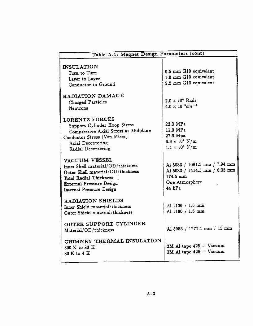
INSULATION Turn to Turn Layer to Layer Conductor to Ground

Table A.l: Magnet Design Parameters (cant)

( I.5 mm GIO equivalent 1.0 mm GIO equident 2.2 mm GlO equivalent.

RADIATION DAMAGE Charged Particles Neutrons

2.0 x 10’ Rads LO x 10%m-2

LORENTZ FORCES Support Cylinder Hoop Stress Compressive Axidai Stress at Midpiane

Conductor Stress (Von LMises j Axial Decenrering Radial Decentering

23.3 MPa /: 11.0 MPa

27.9 Mpa 6.9 x 10’ N/m 1.1 x IO’ N/m

VACUUM VESSEL Inner Shell material/OD/thickness Outer Shell materiai/OD/thickness Total Radial Thickness Jhterual Pressure Design Internal Pressure Design

Al 5083 / 1081.5 mm 1 7.94 mm Al 5083 / 1414.5 mm / 6.35 mm 174.5 mm One Atmosphere 44 kPa

RADIATION SHIELDS Inner Shield materidithickness Outer Shield material/thickness

Al 1100 / 1.6 mm I Al 1100 / 1.6 mm

OUTER SUPPORT CYLINDER Materiai/ODlthickness Al 5083 / 1271.1 mm / 15 mm

CHIMNEY THERMAL INSULATION 300 K to 80 K 80 K to 4 K

3M Al tape 425 + Vacuum 3M Al tape 425 + Vacuum

-

A-3

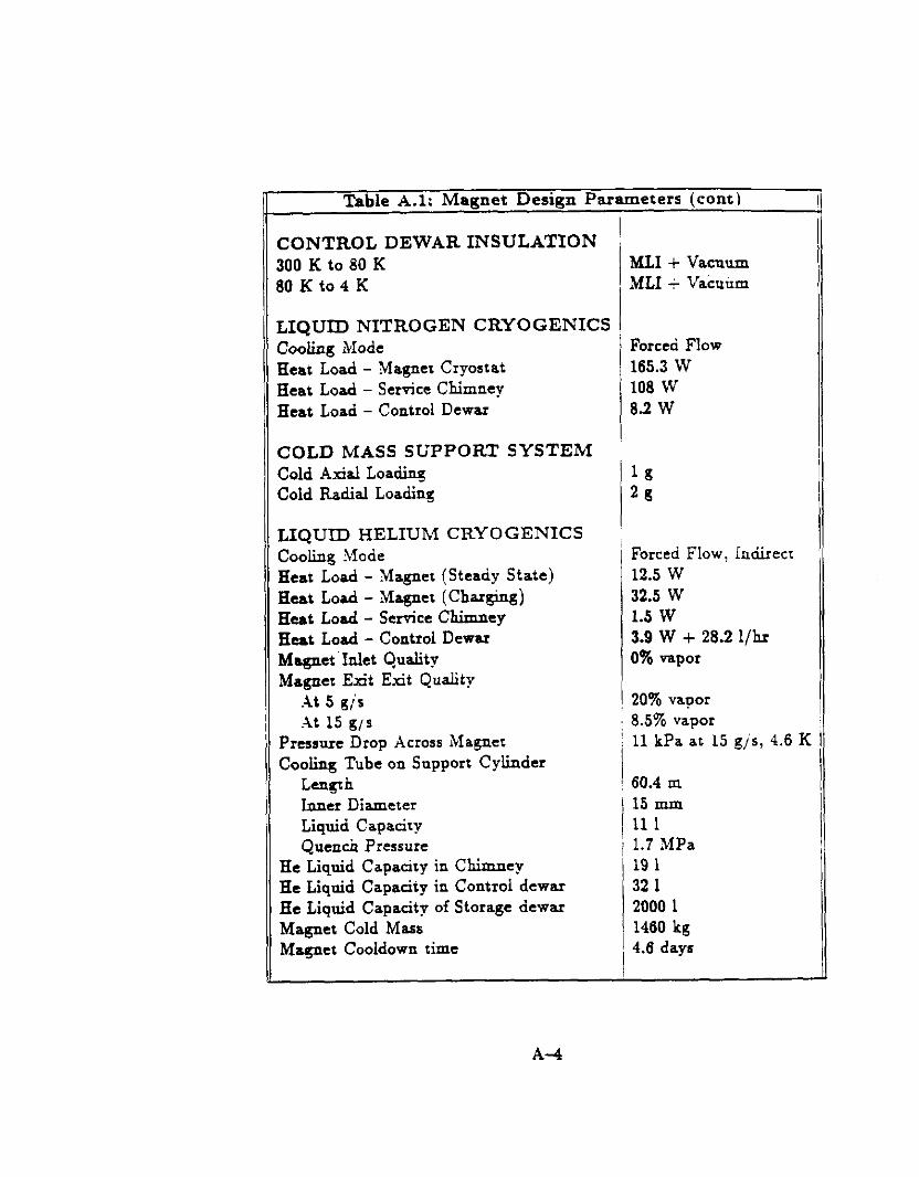
Table A.l: Magnet Design Parameters (cant) I

CONTROL DEWAR INSULATION 300 K to 80 K 50 K to 4 K

LIQUID NITROGEN CRYOGENICS Cooling Mode

Beat Load - Magnet Cryostat

Beat Load - Service Chimney Beat Load - Control Dewar

COLD MASS SUPPORT SYSTEM Cold Axial Loading Cold Radial Loading

LIQUID HELIUM CRYOGENICS Cooling Mode Beat Load - Magnet (Steady State) Beat Load - Magnet (Charging) &at Load - service chimney Beat Load - Control Dewar Magnet. Inlet Quality Magnet Exit Etit Quality

At 5 gis

At 15 g/s

Pressure Drop Across IMagner Cooling Tube on Support Cylinder

LeIlgth Inner Diameter Liquid Capacity Quench Pressure

He Liquid Capacity in Chimney He Liquid Capacity in Control dewar He Liquid Capacity of Storage dewar Magnet Cold Mass Magnet Cooidown time

ML1 -i Vacuum MLI + Vacuum

Forced Flow 165.3 W 108 W 8.2 W

lg 2g

Forced FIow, Indirect ! 12.5 W 32.5 W 1.5 w

3.9 W f 28.2 l/h.r 0% vapor

20% vapor

8.5% vapor

11 kPa at 15 gjs, 4.6 K 1

60.4 m 15 mm

111 1.7 MPa 19 1 321

2000 1 1460 kg 4.6 days

APPENDIX B

FERMILAB SAFETY CONSIDERATIONS

B.l General

The superconducting solenoid, service chimney, control dewar, refrigeration system, energization system, and the protection and control system, will be designed and built in accordance with applicable Fermilab Environment Safety and Health (ES&H) policies. To ensure that this goal is achieved the system will be reviewed by the independent DO Cryogenic Safety Review Panel. This panel will be provided with documentation in order to make recommen- dations to the Research Division head. A signed approval from the Research Division head is required.before the system can be put into operation.

Fermilab ES&H chapter 5032, “Cryogenic System Review”, specifies the various ES&H chapters which must be followed and the documents required. Initial safety review by the DO Cryogenic Safety Panel will have begun prior to the initiation of procurement of the system. This review will be based on the information in this document. After a vendor has been selected, that firm will provide a comprehensive conceptual design for approval by Fermilab. The DO Cryogenic Safety Panel will begin study of this material in depth as part of the overall Fermilab approval of its content. When the complete engineering design is presented by the vendor, the Safety Panel is expected to be able largely to complete its work. If safety-related issues arise at any time in the foregoing process, the vendor must provide calculations, drawings, and test data as required by the Fermilab Safety Panel.

Because the refrigeration, energiaation, and control and protection systems will be designed and installed by Fermilab the safety review of these elements of the system will be paced by the in-house design, fabrication and installation activities of these components.

B-l

APPENDIX C

APPLICABLE CODE REQUIREMENTS

The Department Of Energy and Fermilab have established Environmental, Safety, & Health regulations that apply to all installations and activities at the Laboratory. The magnet system will comply with these ES&H requirements provided that it is designed and fabricated according to the following codes:

ASME Boiler and Pressure Vessel Code

ASME Boiler and Pressure Vessel Code, with reduced safety factor

ASME/ANSI B31 Code Series

CGA Pamphlet P-l

CGA Pamphlet S-l.3

Fermilab ES&H 5031: Pressure Vessels

Fermilab ES&H 5033: Vacuum Vessels

Fermilab ES&H 5031.1: Pressure Piping

Fermilab ES&H 1020: Fermilab/DOE/OSHA/EPA Relationships

Fermilab ES&H 1020: Fermilab/DOE/OSHA/EPA Relationships

ASCE7-88 Building Code Requirements for Minimum Design Loads in Buildings and Other Structures

C-l

APPENDIX D

RADIATION AND INTERACTION LENGTHS

The particles generated by pp collisions at the DO interaction region penetrate the solenoid. In order to calculate the interaction probability of the particle in the solenoid the radiation and interaction lengths of all the materials in the solenoid need to be known. Table D.l shows the radiation and interaction lengths of all the major elements that make up the solenoid. The total radiation length is 0.871, and the total interaction length is 0.189. Table D.l is calculated for particles that are generated at the center of the detector (Z=O) and which penetrate the solenoid at normal incidence (n/Z). The superconductor is assumed to be uniformly distributed over the width of the conductor. The radiation and absorption lengths of the materials that make up the solenoid are shown in Table D.2

For particles which are generated at Z=O, but which are incident on the solenoid at angles other than x/2 radians, the interaction and radiation lengths are shown in Figures D.l and D.2, respectively. In these figures, the incident angle is parametericed as the pseudorapidity 7 given by:

?7 = -In(tan(s/z)),

where 6’ is the scattered angle relative to the incident particle direction. The particles at 7) = 2.0 (0 x 0.27 rod = 15.4O) go through approximately 3.3 radiation lengths, and 0.72 interaction lengths of material in the magnet. Note at large n the discrete effects of the cold mass support system are ignored.

For electron identification, a preshower detector is installed just outside the cryostat of the solenoid. Between the cryostat and the preshower detector, a specially shaped lead sheet is mounted to aid in electron identification and to compensate the response of the preshower detector for the effects of additional material in the solenoid. To make a uniform value of 2 radiation lengths around the central region, as shown in Figure D.3, the thickness of the lead sheet is calculated, taking into account the radiation length of the solenoid. The thickness of this lead sheet is shown in Figure D.4. Because the interaction region is spread out about Z = 0 by about 30 cm total width, it is appropriate to approximate the thickness of this sheet in a few discrete values.

D-l

II Table D.l: Radiation and Interaction Lengths for / Particles Normallv Incident on Solenoid I+ Mate&I Asorption

Length

i

Inner Vacuum Shell Inner Radiation Shield

Outer Radiation Shield Outer Vacuum Shell

Totals

Al Al Al

Cu:NbTi GlO/Epoxy

Al Al Al

0.0172 0.0043 0.0731 0.0187 0.0098 0.0403 0.0043 0.0212

0.1889

Table D.2: Radiation and Interaction Lengths of Selected Materials

Mate&J Xc AI

Aluminum 8.9 cm 37.2 cm Cu/NbTi 1.6 cm 15.0 cm GlO 18.0 cm 45.0 cm

D-2

Radiation length as o function of the pseudorapidity ,or 00 rol.nold

4

‘;iJ 25 5 k? : 2

: 5 5 2 1

0 0.0 0.2 0.4 0.6 0.8 1.0 1.2 1.4 1.6 1.6 2.0 2.2

Pseudorapidity

Figure D.l : Radiation length as a function of psuedorapidity

Interaction length as a function of the pseudorapidity lot 00 Sd.“dd

1.0

-- CM on

0.6

f

1 0.6 f

E =

g 0.4 i c

0.2

0.0 0.0 0.2 0.4 0.6 0.8 1.0 1.2 1.4 1.6 1.6 2.0 2.2

Pseudorapidity

Figure D.2 : Interaction length as B function of psuedorapidit\

Radiation length as a function of the pseudorapidity ,o, 00 sot*rdd

4

G’ 5

f F f 2

E 5 5 s 1

0 0.0 0.2 0.4 0.0 0.6 1.0 1.2 1.4 1.6 1.6 2.0 2.2

Pswdorapldity

Figure D.3: Radiation length as a function of psuedorapidity for a “flat radiation length = 2 Xo” with an extra piece of lead

Shape of the lead for the cara of the aluminum package with Q flat radiation length 2 Xo

I-

250 500 750 low 1250 1500 1750 2000 2250 2500 2750

I dimension of the lead (mm)

Figure D.4: Shape of the lead for a “flat radiation length = 2 X0”

APPENDIX E

CONDUCTOR STABILITY

E.l Conductor Stability

The DO magnet conductor is stabilized with high-purity aluminum and sufficient stabilizer has been included to limit the final peak temperature in the event of a quench, as described in Chapter 11. Because the stored energy of the magnet is smaller than e.g. the Aleph detector solenoid [I] a smaller amount of pure aluminum is required for this purpose than was used for the Aleph conductor. Thus although the current density averaged over the conductor is larger for the DO magnet, the figure of merit pertaining to quench safety, total magnet cold mass divided by magnet stored energy, for the DO magnet (Figure E.l) is not largely dissimilar from Aleph and other thin solenoids.

The amount of high purity aluminum included directly affects the stability of the conductor however. Because the radiation length thickness of the DO magnet was not required to be especially thin as much high purity aluminum as possible was incorporated in the design of the conductor as was permitted by the thickness budget of the magnet and as was judged consistent with overall windabiity of the conductor given the rather small radius of the DO magnet. Given that the conductor current density remains higher than other larger magnets, it is particularly useful to compare the resulting stability margins of the magnet with that of other thin magnets to ensure that the reduction in stabilizer has not jeopardized the performance of the coil.

E.2 Steady-State and Transient Heating

Steady heating in the magnet is not the concern. By assumption such heating, from e.g. conductor joints, or heat radiation and conduction from the cryostat, has been made sufficiently small such that the cooling available to the coil is more than adequate to remove this heat and maintain the coil at the desired low temperature. Care in the design and manufacture of the coil and cryostat, and in the specification of the cryogenic system, can justify this assumption.

Transient heating however can easily degrade the performance of the magnet so that at worst it never reaches its design operating current or, less seriously, enables the magnet to reach full field only after extensive “training”. Transient disturbances, stemming from e.g. energy released by cracking epoxy or inelastic motion of a section of conductor, are generally believed to be the sources of energy that can cause coil performance to be degraded.

E-l

As is well understood, if a quantity of energy is absorbed by a conductor, the final temperature of the conductor is limited only by its enthalpy and any cooling effects available to the conductor. The critical current of the conductor falls with increasing temperature so that~if the temperature begins to rise due to the absorption of heat, at some point the conductor can no longer carry the full current without losses and an increasing fraction of the current begins to generate ohmic heating. This “current sharing” process cascades (unless there is sufficient cooling to prevent it) until the conductor is entirely quenched, ie. has been driven completely normal.

In the absence of any cooling the specific energy sufficient to drive a bare superconductor normal is extremely small. The exact margin is given only by the fraction of the critical current the conductor is carrying before the disturbance occurs. If the conductor is carrying 100% of its critical current it can tolerate no disturbances at all without entering the current sharing mode.

E.3 The MPZ Theory

Superconductor stabilized against flux jumping is typically prepared in a matrix of norrnal- conducting metal. In addition to providing a low-resistance parallel path for the current in the event that some or alI of the current is driven out of the superconductor, this metal adds to the stability of the conductor in two ways. First, it increases the enthalpy available to absorb heating, and second, it provides a conduction path for heat to be carried away from a hot spot into cooler portions of the windings.

This second mechanism is exploited by the MPZ ( “minimum propagating zone”) theory of Wipf [2], Martinelli and Wipf [3], and Wilson and Iwasa [4], to explain the stability margins observed in actual magnets.

The MPZ theory postulates that for all disturbances below a certain critical energy, a transient normal zone in the magnet is created which thereafter decreases in size because the heat generated in the windings driven into the current sharing mode by the disturbance is conducted away from the zone by the stabilizer of the conductor. The initial normal zone created by the disturbance is smaller than the MPZ and does not propagate. For disturbances greater than this critical energy, the normal zone grows in size without limit because the heat generated by the normal windings exceeds the cooling provided by the stabilizer. The zone exceeds the MPZ and propagates.

The theory is relatively straight forward to apply to a winding design that does not involve helium coolant in direct contact with the conductor [5] The magnet windings are ap- proximated by an anisotropic continuum of metal and insulator, the temperature-dependent properties of the materials and the critical properties of the superconductor are supplied, and the size of the largest stable (elliptical) zone where the superconductor has been driven into the current-sharing mode, plus the surrounding shell where the temperature is decreas- ing bath to the bulk of the magnet, is found. The summed energy in the two parts of the

E-2

windings is then calculated by integrating the specific heat of the windings involved over the temperature range specified. This is the minimum energy pulse, the E,,,pz, capable of creating an expanding normal zone in the magnet.

The MPZ energy of an magnet made with a typical Cu:NbTi conductor without extra normal-metal stabilizer and potted into a winding structure is quite small(see figure E-2).

A winding design made with a conductor deliberately stabilized with extra normal metal can have an MPZ energy much larger than that measured in Figure E.2. Following the notation of Wilson we calculate the MPZ of the DO magnet:

E mpr = &d = -% x (eg + eh)

where E, = ~dR~7H,. The normalizing factor E, is just the enthalpy of the winding in the elliptical-shaped “generation” region at B,, where I& is the major axis of the ellipse and Q = (kJk.)‘/‘, with k, and k, the thermal conductivities in the radial and longitudinal directions in the winding, so that CXR, is the minor axis of the zone, and 7H, is the enthalpy in the winding at the temperature 8, (7 is the density). The dimensionless terms ep and eh are integrals from 8, to 9, in the “generating” zone and the “halo” zone of the MPZ. The “generating” zone lies inside the radius R, which contains the conductor driven into the current sharing regime beyond 8, and the “halo” zone lies outside the radius Rs out to a “cold boundary” radius at 6,.

Wilson presents the solution for the sum et = e, + eh as a function of p = (6’,, - 6’,)/& in Figure E.3

E.4 Applying The MPZ Theory

By evaluating p for a given conductor [where one assumes J, falls linearly with temperature so that 8, = B, - (8, - B,)J,,,/J,, and so p = (0, - Bo)J,,,/J~] one finds et from Wilson’s curve, and calculates E, from the parameters appropriate to the magnet in question so that the MPZ energy follows immediately. In what follows a is used to describe the radial thermal conductivity ratio and E the axial thermal conductivity ratio since these are so dissimilar in the DO magnet. Wilson’s term a* is then replaced by ac.

Before inserting numbers, it is helpful to examine the MPZ formula to see how this quantity can be maximized. One notes that et increases nearly linearly with p = (0, - k)J,,,/J, so that one wants to operate the magnet at a temperature tJo as far below the critical temperature of the conductor as practicable, and one wants to minimize the ratio J,,,/J,, i.e. operate at as low a fraction of J, as practicable. These results are intuitively obvious.

The quantity E, is maximized by making ac large, by making 4 large, and by malting 7H, large. A winding design with high turn-to-turn (and layer-to-layer) heat transfer is exceedingly advantageous in increasing (I and l .

E-3

Now K = +6’c - %))I,,

\ ” 1

where X, is the fraction of the windings occupied by conductor and G, = pA*JA/(l - X). A is the fraction of superconductor in the conductor and J,,, is the current density in the superconductor.

Note Rr is maximized by maximizing k,/p; selecting high purity aluminum (so that its BBR 2 1666) one can increase this ratio by an order of magnitude over that for OFHC

copper in a 2T field. In Table E.1 are the values of the various terms evaluated for the CDF test magnet [6],

the CLEO I thin solenoid [7], and the D0 magnet. Because the CDF test magnet is just a single layer coiI and the MPZ radial dimension a% is SO much greater than the coil radial thickness, we use a two-dimensional elliptical volume just as thick as the winding, nen x RiAr, rather than the fully spheroidal volume given by Wilson in E, above.

E.5 Conclusions

The CDF test magnet was quenched at a current of 5000 amperes with a fast energy pulse of 13 Joules. The agreement between this value and the MPZ prediction is instructive; the MPZ result, involving as it does estimations of the various parameters actually pertaining to the coil, cannot be considered more accurate than a factor of two or so, but it can clearly predict the “neighborhood” of stability of a winding design, as it did for the coil in Figure E.2.

We note that the MPZ calculations predict a smaller stability margin for the DO magnet than the CDF test magnet; such is the consequences of a two-layer winding design where a significant thermal barrier must be placed between winding layers. An examination of the results from the CLEO I calculation can reassure us that this reduction is not likely to be critical.

From the table we see that the CLEO I magnet has an MPZ typical of marginally stabilized magnets like that shown in Figure E.2. The CLEO I parameters were evaluated for the magnet operating at 1.0 T, and from the fact that it operated at this level routinely it can be concluded that the spectrum of transients to which it was exposed never exceeded the MPZ energy given in the table. Since it is hard to see how thin magnets which have added stabilizer would be subject to larger transients, assuming they are as carefully made as was CLEO I, they are evidently stable against transients many times larger (evidently by many orders of magnitude) than they actually experience. The successful operating experience with the many aluminum-stabilized solenoids in particle detectors that have been built supports this conclusion; evidently we may conclude that the D0 magnet is sufficiently stabilized for proper operation at fuIl design current.

E-4

References

[l] J.M. Baze, et.al,“Design, Construction and Test of the Large Superconducting Solenoid Aleph”, IEEE Transactions on Magnetics, Vol 24, No. 2, 1988.

[2] Wipf, S.L, Los Alamos Scientific Laboratory Report LA 7275, 1978.

[3] Martinelli, A.P. and Wipf. S.L., Proceedings of the 1972 Applied Superconductivity Conf, Annapolis, IEEE, New York, p 331.

[4] Wilson, M.N., and Iwasa, Y. “Stability of Superconductors Against Localized Distur- bances of Limited Magnitude”, Cryogenics 18, 1978, p 17.

[5] Wilson, M.N., “Superconducting Magnets”, Clarendon Press, Oxford, 1983.

[6] S.Mori, etal., “Construction and Testing of Superconducting Solenoid Magnet Model for Colliding Beam Detector”, Advances in Cryogenic Engineering Vol 27, p 151, Plenum, New York, 1982.

(71 D. Andrews, etal., “A Superconducting Solenoid for Colliding Beam Experiments”, Ad- vances in Cryogenic Engineering, Vo127, ~143, Plenum, New York, 1982.

E-5

Jm I4 J,,, [105A/cm2] x LPlL p [lo-s&n - cm]

Gc IV,4 k [WInKI k [w/~Kl k. W/~Kl a

i @c(B) WI 6 WI & b4 Eo IJI

5000 1500 4825 1.68 1.36 1.35 0.04 0.20 0.062 0.63 0.43 0.57 4.0 19.5 5.0 0.198 90.2 0.373 23 0.5 18 23 0.035 0.153 0.092 0.071 0.022 1.0 0.265 0.092 0.063 0.377 0.035 0.97 0.92 0.86 8.7 8.8 8.3 4.5 4.6 5.1 55.4 0.33 31.6 1.6 2.8 x 10-s 0.59

9 7 6 14 2 x lo-’ 3.5

Table E.l: MPZ Calculation / CDF Test Magnet ] CLEO I Magnet ( I I

DO Magnet

E-a

“e

1 0. -0 .m l - i

Tcmz 0 b I41 1. 00 l . UEOII 1

b 2. m8.s

0 1 IQ 100 1000

Stored Enrrw WI

Figure E.l: Stored Energy per Unit %old Mass vs. Stored Energy for Various Detector

Magnets.

Froclim 01 ulcicd cvrml I I I,

Figure E.2: MPZ energy for an epoxy-filled magnet. The points are measured values, the curve is the MPZ theory.

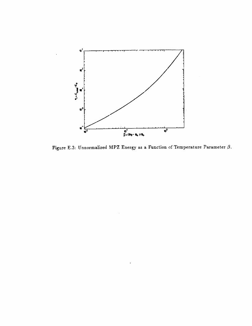
Figure E.3: Unnormalized MPZ Energy as a Function of Temperature Parameter p.

APPENDIX F

ALIGNMENT CONSIDERATIONS

F.l General Remarks

The solenoid will be mounted in the warm bore of the CC cryostat and its final position fixed using fiducial marks placed on the outer vacuum jacket of the magnet cryostat which predict the location of the coil inside after it is cooled and energized. In general it is possible to measure the locations of such fiducials to 0.25 mm (0.010 in) or so in x and y, and perhaps a as well, in some coordinate system that can be referred to the remainder of the detector and ultimately to the colliding beams (e.g. a system based on the detector center beam).

By specifying that the total radial .uncertainty in the location of the coil inside the cryostat does not exceed &5mm, then the angular uncertainty in the direction of the field axis does not exceed Q s 2 x 5mm/2.56m = 4 mrad. The survey tolerances (0.25 mm) do not appreciably increase this when the field is referenced to the TeVatron.

In order that the initial misalignment not significantly degrade over time (due to thermal or magnetic cycling) we specify that the magnet cold mass support system locate the coil reproducibly to e.g. twice the initial placement accuracy, f 0.5 mm, so that the total misalignment never exceed zt 5 mm.

The silicon microstrip and scintillator fiber tracking systems will be mounted in the bore of the magnet and aligned to it so that the axes of the trackers and the magnetic field are parallel to the same tolerances. Thus the maximum misalignment between the axis of the field and the axis of these trackers will also not exceed x 4 mrad.

In what follows we show that this tolerance is sufficient to preserve necessary alignment of the magnet both for machine requirements and for tracking requirements.

If it is determined that the field of the magnet is not sufficiently accurately known from the manufacturer’s specifications, then the field can be mapped to find the field axis with respect to fiducial marks on the cryostat. In this eventuality, the final angular misalignment between the magnetic field and the TeVatron or the tracking system can be reduced to a fraction of 4 mrad.

F.2 TeVatron Requirements

It is necessary that the solenoid not generate closed orbit distortions in excess of 1.0 x 10-s m (G. Goderre, FNAL AD, private communication) in the arcs of the machine after the stored beams leave the interaction point. While a fringing solenoidal field concentric with the beam and parallel to it cannot cause beam steering, one rotated by an angle a about

F-l

any axis perpendicular to the beam can. If the magnet is in fact misaligned by such an angle Q the integral

/Bdl= jB.tonodl=6B~Z

is nonzero along the beam path, and this integral generates a net steering force on the beam. Here we write B. for the average of the field B,tancz over the magnet length, and Z the length over which this average filed is effective. Note that if the magnet is aligned to the beam so that Q is zero, the beam need not even be precisely concentric with the field since the resulting field integral remains zero as long as the field at one end is symmetric with the field at the other.

The closed orbit distortion amplitude of the stored beam at point k generated by a non-zero “error field” integral SB.Z at the interaction point IP is given by

where prp is the beta function at the interaction point, pa the beta function at point k, and Bg is the beam guide field strength and p the machine radius.

Since for a beam particle of momentum p the guide field obeys p = 0.3B,p, we have at injection, B,p = 150/.3 = 5002’~~ and at flattop, B,p = 900/.3 = 3000Tm.

At the interaction point, p = 2m, and in the arcs p = 10Om. The condition that the closed orbit distortions not exceed 1.0 x IO-%n then implies that the “error field” integral obey

6B z < 2 x 10-3Bs~ e

&am’

Now Bp is smallest at injection, so we find we must have for this most severe css.e

b-B,Z < 0.0707 Tm.

We approximate the actual “error field” integral for the solenoid misaligned by an angle LZ as a 2 Tesla field effective over the physical length of the coil, 2.56 m,

6B.Z = Bdl z J 2.OT x 2.56~~ x tanu.

Then we have

tana < z = 0.0138,

so

CY < 14mrad.

F-2

Note that during collisions @up is smaller by a factor of about eight and the guide field term is larger by a factor of six so that during collisions the condition is easily met.

The support system of the magnet must maintain the rotational alignment of the magnet to the tolerance obtained in order to be useful at the TeVatron. For safety, we choose a specitication that guarantees the misalignment to be substantially less.

F.3 Tracking System Requirements

Because a direct measurement of pl is provided by the tracking system and the magnetic field of the solenoid, is it necessary to examine how residual small relative misalignments between the trackers and the magnetic field will affect the accuracy of this measurement.

(It is noted that the tracking system is likely to participate in part of the Level 1.5 trigger so it will ultimately be necessary to consider how misalignment of this system can bias such a trigger. For example, if the tracking system is part of a pA threshold estimation for the trigger, then if it is displaced laterally a cos+ - dependance on the trigger threshold would result. Additionally if the tracking system is to be used to obtain track stubs or segments for the trigger, then the effect of misalignments of the field on this trigger must be examined. Such trigger-dependent topics are not considered in the following. They may well generate constraints that are more severe than those discussed herein).

Studies have been made of the resolution in pL promised by the full upgrade silicon and scintillation-fiber tracker systems. The results are eta-dependent and have been estimated

, for event vertices at z = 0 and for z > 30 (see Figure F.3). The error in pl increases with eta and is larger for z > 30, but to key on the most

stringent needs, we quote the result for eta = 0 and z = 0:

- = 0.016 @ O.O02Pl, PI

where the first term describes multiple scattering and the second is due to measurement errors. Perfect knowledge of a perfectly aligned uniform field was used to develop this result, and no pattern recognition confusion was included. The undulations in the curves stem from the transitions in coverage between the ends of the tracker barrels and the discs at the specific values of eta involved.

For a particle with e.g. pL = 1 Gev/c, roughly the lower limit desired in DO Upgrade, the “geometry” term is 2 x 10T3.

For a particle moving in a magnetic field we have,

0.3 x B. PL = K

where K = curvature = l/R. Then

F-3

U2(Pl) 4%) 4K) -z- =7+7

describes how the measurement uncertainties contribute to u(pl) if the uncertainties in the knowledge of the values of the field are allowed to contribute. It is reasonable to require that these additional uncertainties not exceed 10% of those from the determination of the curvature, i.e.,

dB=) - 5 2 x lo-* B.

at 1 GevJc. If the DO upgrade tracking system is misaligned with respect to the field by a small angle

Q, then an uncertainty in the value for B, is generated:

B&d * = BMmiM’co+) I

2 BnaniM’[l. - ~zr’/2]. I

Now if

AB. = By” - By’“, then

AB, = -q2B-iM~

; ,of ABz -a2 - = -.

B* 2

For a = 4 mrad,

A& - = 8 x 10-6.

B*

This remains comfortably smaller than the limit specified above.

F.4 Vertex Resolution Due to Misalignment

Misalignment of the tracking system with respect to the magnetic field can also introduce errors in the determination of the a of a secondary interaction vertex.

If the tracking system is perfectly aligned to the magnetic field then B, and Bh are nominally sero. However, if the magnet axis is misaligned by an angle Q then B, and B+ are

F-I

2 B, x CI. These uncertainties, while they do not contribute directly to the measurement of pl for any track, do contribute to the uncertainty of the location of the z of e.g. a secondary vertex.

Crudely, if a straight line is fit to a trajectory ~1 which is actually curving due to a field Bl = B, x Q, then an angular uncertainty in the trajectory of the track is introduced that can be characterized by the total angle of bend of the track at its midpoint.

The curvature is not large: for even a pii = 1 Gev/c track, R = p/(0.3 x BL = l/O.3 x 2 x 4 x 10-s = 417 meters. Taking the radial dimension S N 0.15~7~ of the silicon tracker as the characteristic length, then

68 = 0.3 x Bl x S/q,, or

68 = 1.8z10-4. Such an angular mismeasurement would contribute an error at the vertex of AZ = R x A@ = 2.7~10~~ = 27 microns. The resolution of the tracker, for e.g. B + P + /.L~L, calculated without this effect, has been given [l] as cr, = 220 microns. Evidently the field misalignment Q = 4 mrad will not significantly spoil this resolution.

We conclude that if the magnet is constructed to readily-achieved engineering tolerances then the tracker systems can be installed into it and aligned to fiducials on it using standard optical survey techniques. The contribution to uncertainties in the measurements of particle pl, or to the z coordinate of secondary vertices from errors arising from this process are entirely negligible.

Indeed, as was with the case for the CDF solenoid[2], even if the misalignment angle has been determined quite precisely by a field-mapping exercise it can be entirely ignored.

By an alternate viewpoint, nonuniformities in B, stemming from the design of the magnet itself exceed a few parts in one hundred for extreme trajectories in the tracker, so the additional nonuniformity as estimated in the foregoing due to a small misalignment of the magnet axis is entirely negligible.

References

[I] DBNote 1733, E823 DBUpgrade, May 1993

[2] C. Newman-Holmes, .&al., “Measurement of the Magnetic Field of the CDF Magnet”, Nuclear Instruments and Methods in Physics Research, A2’74, 1989, pp 443-451.

F-5

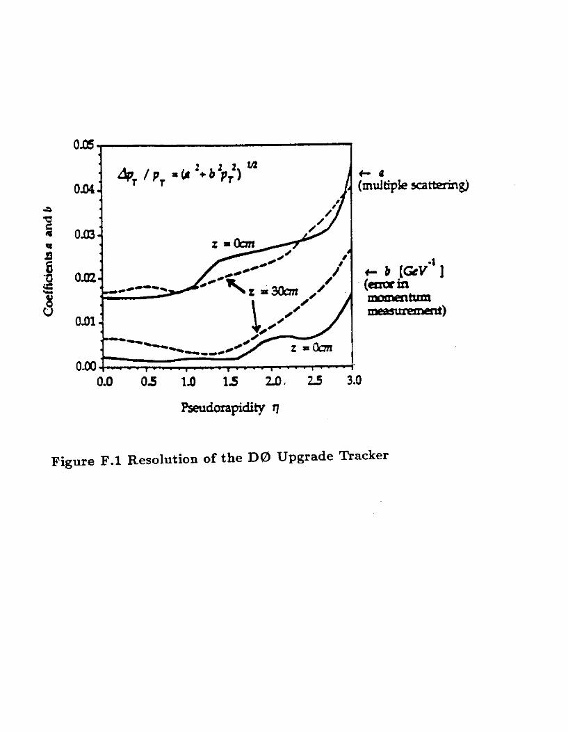
ow bpr /Pr =(1 w:) Ia A I’ / I

0.03

0.02

0.0 05 1.0 15 Lo, 25 3.0

-dorapidity rl

t b [GCY‘I ] .( euuin nBmxntum -1

Figure F.l Resolution of the D0 Upgrade Tracker

APPENDIX G

SUPPORTING DOCUMENTS

During the preparation of this conceptual design, a number of engineering notes were written which provide greater detail on a given topic than the results summarized herein. These notes are kept on file in the DO Engineering Note library.

NOTE

3823.111-EN-338

TITLE

3823.111-EN-341

3823X1-EN-342

3823.111-EN-343

3823.111-EN-344

3823.111-EN-345

3823.111-EN-348

3823.111-EN-349

3823.111-EN-350

LHe Flow Regime/Pressure Drop for DO Solenoid at Steady State Conditions

DO Solenoid: Pressure Ratings for Some Chimney and Control Dewar Components

Chimney LN2 Radiation Shield Attachment Area Calculation

DO Solenoid: Rectangular LHe Supply Tubing, Misc. Information

Heat Load Calculations for Solenoid Chimney

Solenoid Insulating Vacuum Vessel: Relief Path Capacity Calculations

Vacuum Pumping Calculations for the DO Solenoid

Thermal Contraction Analysis for the D0 Solenoid Chimney

DO Solenoid Current Leads

AUTHOR

Russ Rucinski

Russ Rucinski

Russ Rucinski

Russ Rucinski

Russ Rucinski

Russ Rucinski

Russ Rucinski

Russ Rucinski

Russ Rucinski

DATE

313193

5125193

5126193

5126193

5126193

5126193

812193

10/l/93

10/4/93

G-l

NOTE TITLE AUTHOR DATE

3823.111-EN-351

3823.111.EN-352

3823.111-EN-353

3823.111-EN-354

3823.111-EN-355

3823.111-EN-356

3823.111-EN-358

3823.111-EN-359

3823.111-EN-360

3823.111-EN-361

3823.111-EN-362

3823.111-EN-365

3823.111-EN-366

3823.111-EN-367

Control Dewar Subcooler Heat Exchanger Calculations

Control Dewar LHe Reservoir Sizing

Control Dewar Secondary Vacuum Container

DO Solenoid Chimney Open Issues

DO Solenoid Control Dewar Open Issues

DO Solenoid Chimney Routing Clearances

Cold Mass Support System for the DO Solenoid

Cold Mass Cool Down Calculation for the D0 Solenoid

DO Solenoid Cold Mass Steady State Operation: Helium Flow Calculation and Cold Mass Temperature Profile

Heat Loads in the D0 Solenoid Cryostat

A Collection of Calculations on the DO Solenoid Cryostat

Lifetime Radiation Levels in DO Beta

DO Beta Magnet Decentering Forces: An Image Dipole Approach

DO Beta Magnet Decentering forces: An Image Solenoid Approach

Russ Rucinski

Russ Rucinski

Russ Rucinski

Russ Rucinski

Russ Rucinski

Russ Rucinski

Bruce Squires

Bruce Squires

Bruce Squires

Bruce Squires

Bruce Squires

R. P. Smith

R. P. Smith

R. P. Smith

10/4/g:

10/4/g:

10/4/g:

10/4/g:

10/4/g:

10/4/g:

8/g/93

7127 19:

7/28/g:

9 /g/93

g/3/93

10/14/c

10/30/c

11/20/c

G-2

NOTE

3823.111.EN-368

3823.111-EN-369

3823.111-EN-370

3823.111.EN-371

3823.111-EN-372

3823.111.EN-373

3823.111-EN-374

3823.111.EN-379

3823.111-EN-380

3823.111-EN-404

3823.111.EN-405

TITLE

Charging and Discharging the DO Beta Magnet

A Superconducting Scoping Study for the DO Beta Magnet

DO Beta Magnet Alignment Considerations

DO Solenoid Chimney Fabrication Plan

DO Solenoid LN2 Shield

D0 Chimney Lead Quench Detection for Beta Solenoid

Energy Losses in the DO Beta Solenoid Cryostat Caused by Current Changes

Loss of Vacuum Calculation for the DO Solenoid

Aluminum Stabilizer for the DO Magnet Superconductor

Beam Heating in the DO Solenoid

Revised Lifetime Radiation Levels in DO Beta

AUTHOR

R. P. Smith

R. P. Smith

R. P. Smith

Russ Rucinski

A. M. Stefanik

Age Visser

Age Visser

Bruce Squires

R. P. Smith

R. P. Smith

R. P. Smith

DATE

5128193

3131193

6128193

815193

8/g/93

10/l/93

10/l/93

2117194

11/6/93

l/19/94

10/28/93

G-3

Conceptual Design of a 2 Tesla Superconducting Solenoid ...lss.fnal.gov/archive/tm/TM-1886.pdfFermi...

Documents

Transcript of Conceptual Design of a 2 Tesla Superconducting Solenoid ...lss.fnal.gov/archive/tm/TM-1886.pdfFermi...