David Salzberg 4001 N. Fairfax Dr,  Suite 400, M/S 175 Arlington, VA 22203, USA 

• Many hydrographic surveys tried to idenIfy the secondary sources.   

•  No evidence for a landslide of the scale to produce the observed tsunami 

•  Splay faults were idenIfied in the accreIonary wedge  • While there is direct evidence of slip on the splay faults (no before and aOer imaging, just aOer the fault), the occurrence of aOershocks at the locaIon of the splay faulIng indicate splays were acIve during the earthquake. 

• LocaIon of splay is consistent with tsunami arrival Imes. 

• Tsunami arrived early: clocks at the Banda Aceh mosque stopped at 8:25 local Ime, or 26 minutes aOer the earthquake rupture in an area that is at least 10 miles (10 minutes travel Ime) from the nearest coast.  Conclusion: Tsunami arrived at nearest coast no later than 08:15, or 16 minutes travel Ime (10 minutes early). 

• Tsunami was about three to five Imes too big (based on far‐field source).  Predicted heights, based on the fault dislocaIon model  are on the order of 10 meters, but observed run‐ups were 30 to 50 meters along the west coast of the Aceh province. 

• These items strongly suggest some type of secondary source, such as an induced landslide or secondary splay fault.     

Conceptual Basis for Using the T-Phase:

Walker et al (1992) studied T-phase from multiple, large earthquakes, some of which where tsunamigenic earthquakes are much richer in high frequency (f>30 hz) than typical events. Using data recorded at the modern IMS hydrophones at Diego Garcia from more recent earthquakes (for example, Northern Sumatra, Nias Islands), I have previously demonstrated that those earthquakes that produce significant tsunamis are much richer in 60 Hz and above energy. For example, spectrograms from the the two largest earthquakes in the last 40 years, the Northern Sumatra, and Nias Islands earthquakes (Mw = 9.1 and 8.7 respectively) are shown below. The Northern Sumatra earthquake generated a devastating tsunami; the tsunami from the Nias Island earthquake was more modest. Examining the spectral content, it is clear that the T-phase from the Northern Sumatra earthquake was much richer in high-frequency energy than that for the Nias Island earthquake.

The figure above shows spectrograms of the 2004 Northern Sumatra Mw=9.1 and 2005 Nias Islands (Mw 8.7) earthquake. Note that the Northern Sumatra earthquake is much richer in high-frequency T-phase energy than is the Nias Island earthquake.

Walker et al (1992) hypothesized that the higher frequency energy in the observed T-phases may be the result of alternate mechanisms for tsunamigenisis, such as slumping/landslides, liquefaction, etc. However, a simpler explanation is that the frequency content of the T-phase primarily results from analestic attenuation within the solid earth. The concept is that the tsunamigenic earthquakes involve extremely shallow rupture, which results in less attenuation (and thus higher frequency content). The extreme shallow rupture (either from direct continuation of the rupture or a secondary rupture, such as splay faulting, which according to our model, results in the high-frequency T-phase, would also produce a high-amplitude, short-wavelength coseismic displacement. That displacement, coupled with the longer wavelength displacement from the primary (deeper) displacement, produces the tsunami. Because the shallow source produces a a shorter wave-length signal, it propagates as a shallow-water wave in the shallow (near coast) waters; it is deeper water, it disperses.

Current State of Tsunami DetecIon System 

Synthetic Seismogram Synthetic Displacement Modeled T-Phase Spectra

Unlike seismic, T‐Phase can image shallow/splay rupture  

The figures to the right show synthetic seismograms, coseismic displacement, and the predicted T-phase spectra for a model where a primary rupture (shown in blue) excites splay faulting in the accretionary wedge. The model assumed identical slip for the primary and splay faulting, but much weaker shear modulus (1/100th in the sediments versus the hard rock). Seismically, the splay fault is 1/100th the amplitude of the primary rupture, though the coseismic displacement is much larger for the splay faulting. The T-phase is able to see both the primary rupture and the splay fault: the primary rupture dominates at low frequencies (<30 Hz), whereas the splay fault T-phase is dominant at higher frequencies.

Data Analysis of Sumatra Aftershocks: Splay faults and spectral slopes

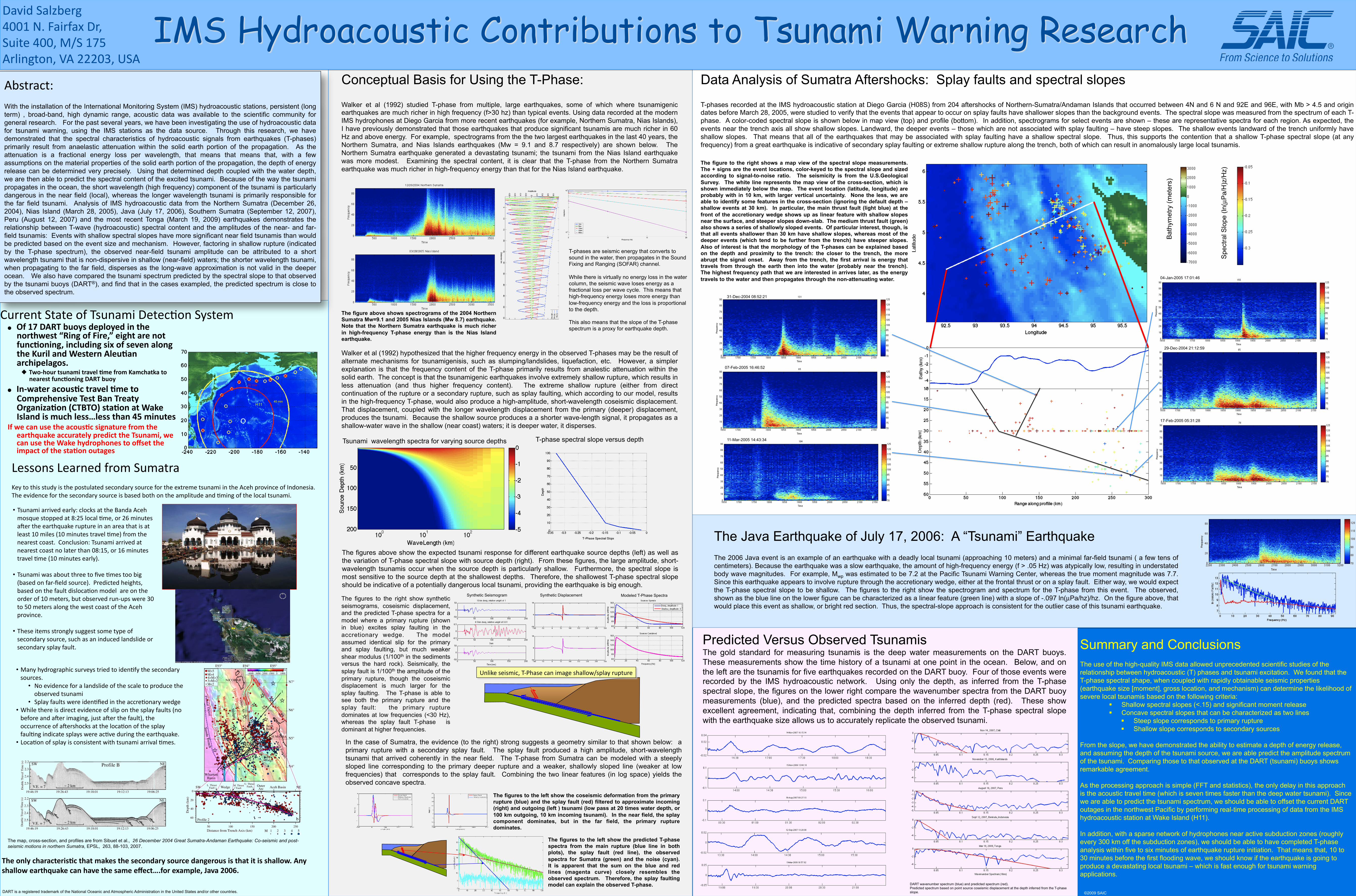
T-phases recorded at the IMS hydroacoustic station at Diego Garcia (H08S) from 204 aftershocks of Northern-Sumatra/Andaman Islands that occurred between 4N and 6 N and 92E and 96E, with Mb > 4.5 and origin dates before March 28, 2005, were studied to verify that the events that appear to occur on splay faults have shallower slopes than the background events. The spectral slope was measured from the spectrum of each T-phase. A color-coded spectral slope is shown below in map view (top) and profile (bottom). In addition, spectrograms for select events are shown – these are representative spectra for each region. As expected, the events near the trench axis all show shallow slopes. Landward, the deeper events – those which are not associated with splay faulting – have steep slopes. The shallow events landward of the trench uniformly have shallow slopes. That means that all of the earthquakes that may be associated with splay faulting have a shallow spectral slope. Thus, this supports the contention that a shallow T-phase spectral slope (at any frequency) from a great earthquake is indicative of secondary splay faulting or extreme shallow rupture along the trench, both of which can result in anomalously large local tsunamis.

The figure to the right shows a map view of the spectral slope measurements. The + signs are the event locations, color-keyed to the spectral slope and sized according to signal-to-noise ratio. The seismicity is from the U.S.Geological Survey. The white line represents the map view of the cross-section, which is shown immediately below the map. The event location (latitude, longitude) are probably with in 10 km, with larger vertical uncertainty. None the less, we are able to identify some features in the cross-section (ignoring the default depth – shallow events at 30 km). In particular, the main thrust fault (light blue) at the front of the accretionary wedge shows up as linear feature with shallow slopes near the surface, and steeper slopes down-slab. The medium thrust fault (green) also shows a series of shallowly sloped events. Of particular interest, though, is that all events shallower than 30 km have shallow slopes, whereas most of the deeper events (which tend to be further from the trench) have steeper slopes. Also of interest is that the morphology of the T-phases can be explained based on the depth and proximity to the trench: the closer to the trench, the more abrupt the signal onset. Away from the trench, the first arrival is energy that travels from through the earth then into the water (probably near the trench). The highest frequency path that we are interested in arrives later, as the energy travels to the water and then propagates through the non-attenuating water.

Bat

hym

etry

(met

ers)

Spe

ctra

l Slo

pe (l

n(µP

a/H

)z/H

z)

31-Dec-2004 08:52:21

07-Feb-2005 16:46:52

11-Mar-2005 14:43:34

04-Jan-2005 17:01:46

29-Dec-2004 21:12:59

17-Feb-2005 05:31:28

The Java Earthquake of July 17, 2006: A “Tsunami” Earthquake The 2006 Java event is an example of an earthquake with a deadly local tsunami (approaching 10 meters) and a minimal far-field tsunami ( a few tens of centimeters). Because the earthquake was a slow earthquake, the amount of high-frequency energy (f > .05 Hz) was atypically low, resulting in understated body wave magnitudes. For example, Mwp was estimated to be 7.2 at the Pacific Tsunami Warning Center, whereas the true moment magnitude was 7.7. Since this earthquake appears to involve rupture through the accretionary wedge, either at the frontal thrust or on a splay fault. Either way, we would expect the T-phase spectral slope to be shallow. The figures to the right show the spectrogram and spectrum for the T-phase from this event. The observed, shown as the blue line on the lower figure can be characterized as a linear feature (green line) with a slope of -.097 ln(µPa/hz)/hz. On the figure above, that would place this event as shallow, or bright red section. Thus, the spectral-slope approach is consistent for the outlier case of this tsunami earthquake.

The map, cross-section, and profiles are from Sibuet et al., 26 December 2004 Great Sumatra-Andaman Earthquake: Co-seismic and post-seismic motions in northern Sumatra, EPSL, 263, 88-103, 2007.

Abstract: With the installation of the International Monitoring System (IMS) hydroacoustic stations, persistent (long term) , broad-band, high dynamic range, acoustic data was available to the scientific community for general research. For the past several years, we have been investigating the use of hydroacoustic data for tsunami warning, using the IMS stations as the data source. Through this research, we have demonstrated that the spectral characteristics of hydroacoustic signals from earthquakes (T-phases) primarily result from anaelastic attenuation within the solid earth portion of the propagation. As the attenuation is a fractional energy loss per wavelength, that means that means that, with a few assumptions on the material properties of the solid earth portion of the propagation, the depth of energy release can be determined very precisely. Using that determined depth coupled with the water depth, we are then able to predict the spectral content of the excited tsunami. Because of the way the tsunami propagates in the ocean, the short wavelength (high frequency) component of the tsunami is particularly dangerous in the near field (local), whereas the longer wavelength tsunami is primarily responsible for the far field tsunami. Analysis of IMS hydroacoustic data from the Northern Sumatra (December 26, 2004), Nias Island (March 28, 2005), Java (July 17, 2006), Southern Sumatra (September 12, 2007), Peru (August 12, 2007) and the most recent Tonga (March 19, 2009) earthquakes demonstrates the relationship between T-wave (hydroacoustic) spectral content and the amplitudes of the near- and far-field tsunamis: Events with shallow spectral slopes have more significant near field tsunamis than would be predicted based on the event size and mechanism. However, factoring in shallow rupture (indicated by the T-phase spectrum), the observed near-field tsunami amplitude can be attributed to a short wavelength tsunami that is non-dispersive in shallow (near-field) waters; the shorter wavelength tsunami, when propagating to the far field, disperses as the long-wave approximation is not valid in the deeper ocean. We also have compared the tsunami spectrum predicted by the spectral slope to that observed by the tsunami buoys (DART®), and find that in the cases exampled, the predicted spectrum is close to the observed spectrum.

Lessons Learned from Sumatra Key to this study is the postulated secondary source for the extreme tsunami in the Aceh province of Indonesia.  The evidence for the secondary source is based both on the amplitude and Iming of the local tsunami.   

H11 45 min

30 min

●  Of 17 DART buoys deployed in the northwest “Ring of Fire,” eight are not func@oning, including six of seven along the Kuril and Western Aleu@an archipelagos. ◆ Two‐hour tsunami travel @me from Kamchatka to 

nearest func@oning DART buoy 

●  In‐water acous@c travel @me to Comprehensive Test Ban Treaty Organiza@on (CTBTO) sta@on at Wake Island is much less…less than 45 minutes 

If we can use the acous@c signature from the earthquake accurately predict the Tsunami, we can use the Wake hydrophones to offset the impact of the sta@on outages 

The only characteris@c that makes the secondary source dangerous is that it is shallow. Any shallow earthquake can have the same effect….for example, Java 2006.  

T-phases are seismic energy that converts to sound in the water, then propagates in the Sound Fixing and Ranging (SOFAR) channel.

While there is virtually no energy loss in the water column, the seismic wave loses energy as a fractional loss per wave cycle. This means that high-frequency energy loses more energy than low-frequency energy and the loss is proportional to the depth.

This also means that the slope of the T-phase spectrum is a proxy for earthquake depth.

The figures to the left show the coseismic deformation from the primary rupture (blue) and the splay fault (red) filtered to approximate incoming (right) and outgoing (left ) tsunami (low pass at 20 times water depth, or 100 km outgoing, 10 km incoming tsunami). In the near field, the splay component dominates, but in the far field, the primary rupture dominates.

The figures to the left show the predicted T-phase spectra from the main rupture (blue line in both plots), the splay fault (red line), the observed spectra for Sumatra (green) and the noise (cyan). It is apparent that the sum on the blue and red lines (magenta curve) closely resembles the observed spectrum. Therefore, the splay faulting model can explain the observed T-phase.

In the case of Sumatra, the evidence (to the right) strong suggests a geometry similar to that shown below: a primary rupture with a secondary splay fault. The splay fault produced a high amplitude, short-wavelength tsunami that arrived coherently in the near field. The T-phase from Sumatra can be modeled with a steeply sloped line corresponding to the primary deeper rupture and a weaker, shallowly sloped line (weaker at low frequencies) that corresponds to the splay fault. Combining the two linear features (in log space) yields the observed concave spectra.

DART wavenumber spectrum (blue) and predicted spectrum (red). Predicted spectrum based on point source coseismic displacement at the depth inferred from the T-phase slope.

Tsunami wavelength spectra for varying source depths T-phase spectral slope versus depth

The figures above show the expected tsunami response for different earthquake source depths (left) as well as the variation of T-phase spectral slope with source depth (right). From these figures, the large amplitude, short-wavelength tsunamis occur when the source depth is particularly shallow. Furthermore, the spectral slope is most sensitive to the source depth at the shallowest depths. Therefore, the shallowest T-phase spectral slope should be indicative of a potentially dangerous local tsunami, providing the earthquake is big enough.

Predicted Versus Observed Tsunamis The gold standard for measuring tsunamis is the deep water measurements on the DART buoys. These measurements show the time history of a tsunami at one point in the ocean. Below, and on the left are the tsunamis for five earthquakes recorded on the DART buoy. Four of those events were recorded by the IMS hydroacoustic network. Using only the depth, as inferred from the T-phase spectral slope, the figures on the lower right compare the wavenumber spectra from the DART buoy measurements (blue), and the predicted spectra based on the inferred depth (red). These show excellent agreement, indicating that, combining the depth inferred from the T-phase spectral slope with the earthquake size allows us to accurately replicate the observed tsunami.

Summary and Conclusions

The use of the high-quality IMS data allowed unprecedented scientific studies of the relationship between hydroacoustic (T) phases and tsunami excitation. We found that the T-phase spectral shape, when coupled with rapidly obtainable seismic properties (earthquake size [moment], gross location, and mechanism) can determine the likelihood of severe local tsunamis based on the following criteria:

  Shallow spectral slopes (<.15) and significant moment release   Concave spectral slopes that can be characterized as two lines

  Steep slope corresponds to primary rupture   Shallow slope corresponds to secondary sources

From the slope, we have demonstrated the ability to estimate a depth of energy release, and assuming the depth of the tsunami source, we are able predict the amplitude spectrum of the tsunami. Comparing those to that observed at the DART (tsunami) buoys shows remarkable agreement.

As the processing approach is simple (FFT and statistics), the only delay in this approach is the acoustic travel time (which is seven times faster than the deep water tsunami). Since we are able to predict the tsunami spectrum, we should be able to offset the current DART outages in the northwest Pacific by performing real-time processing of data from the IMS hydroacoustic station at Wake Island (H11).

In addition, with a sparse network of hydrophones near active subduction zones (roughly every 300 km off the subduction zones), we should be able to have completed T-phase analysis within five to six minutes of earthquake rupture initiation. That means that, 10 to 30 minutes before the first flooding wave, we should know if the earthquake is going to produce a devastating local tsunami – which is fast enough for tsunami warning applications.

DART is a registered trademark of the National Oceanic and Atmospheric Administration in the United States and/or other countries. ©2009 SAIC