Concepts of ThermodynamicsProf. Suman Chakraborty

Department of Mechanical EngineeringIndian Institute of Technology, Kharagpur

Lecture – 57Thermodynamic Relationships

We have discussed about various facets of laws of thermodynamics so far but what we

have not discuss so, far about the ways in which we can characterize or determine

properties. Because the manifestation of various laws of thermodynamics essentially

culminates in terms of calculating the differences in certain properties like entropy,

enthalpy, internal energy like that. Many of these properties are not directly measurable.

So, if they are not directly measurable, they could be indirectly predicted by means of

certain other properties which could be related to the non measurable properties and

these kinds of relationships are called as thermodynamic property relationships or in

general Thermodynamics Relationships.

(Refer Slide Time: 01:21)

So, in thermodynamic relationships we use essentially partial differential calculus or

calculus of partial derivatives to predict the derivatives of measurable or non measurable

properties in terms of one in terms of the other; so, to do that we will essentially establish

certain mathematical backgrounds. Let us say that there is a function z which is a

function of x and y, function of two variables. Why we take such a function of two

variables what is the thermodynamic motivation? For a simple compressible pure

substance if you know two independent intensive properties you can identify the state.

So, these two variables can essentially identify the thermodynamic state. So, this x and y

generically could be pressure, volume temperature, internal energy enthalpy whatever if

they are independent a property can be described as a function of that so you can write.

So, let us call this as M and let us call this as N. Assuming the second order partial

derivative to be continuous we can write right.

So, in the second order partial derivative is continuous, then it does not matter whether

you differentiate with respect to y first or with respect to x first so; that means, from so

this is M and this is N. So, from here we can conclude. So, when you are differentiating

with respect to y, we are essentially fixing x and when we are differentiating with respect

to x partially we are essentially fixing y. So, this is an important outcome.

So, we will write it at one corner of the board because we will use it for our derivations.

So, if z is a function of x and y and d z is M d x plus N d y, then ok. So, this is the first

thing. The second important interesting question is how does the chain rule work for

partial derivatives? The chain rule of derivatives ordinary derivatives that dy dx into dx

dy is equal to 1 right. That kind of a chain rule how does it work for partial derivatives?

(Refer Slide Time: 06:25)

So, we start with so dz. Now, you can also write x as a function of y and z right. So, this

x is a function of y and z. So, dx this you can write. So, you can write dz ok. So, this part

of the board is not visible please show it in the camera yes. So, then you can write. So,

you can compare this term with this term and you can club these two together.

So, if you compare these two terms the first observation that you have is del z del x at

constant y ok. So, it is intuitive, but it follows from rigorous derivation that the inverse of

right the derivative of x with respect to z is 1 by the derivative of z with respect to x.

Also by comparing the coefficients of dy, the boxes which are marked with yellow color.

So, you can have this is 0. So, coefficient of dy this is the coefficient of dy in the right

hand side and coefficient of dy in the left hand side is 0.

So, you can write and del z del y is 1 by del y del z t from the previous expression. So,

from here we can arrive at partial derivative of z with respect to x into partial derivative

of x with respect to y partial into partial derivative of y with respect to z, intuitively by

chain rule this would have been 1 right, but it is actually minus 1. So, this result is very

important and we will use this carefully. So, with the mathematical background

established by this one and these two equations we will now consider how to apply this

for thermodynamics relationships. So, out of the thermodynamics relationship the

combination of first law and second law, give us two important one the two Tds

relationships. So, we will start with that.

(Refer Slide Time: 12:23)

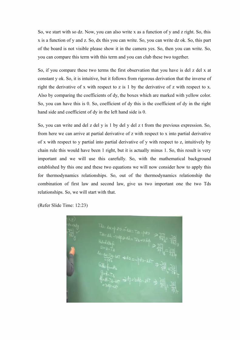
So, you have Tds is equal to d u plus pdv. So, you can cost it in these way dz is equal to

M d x plus N d y by write noting that du is equal to Tds minus pdv ok. Then you have

Tds is equal to d h minus vdp; that means, dh is equal to Tds plus vdp that is also of the

form M d x plus N d y.

Now, to develop two more forms like this we will use the definition of two new

functions, one is called as Helmholtz function and other is called Gibbs function. So, the

Helmholtz function a is equal u minus Ts, what is this also called is the Helmholtz free

energy. We have done exergy analysis and you have seen that the energy that is freely

available to make the most out of a change of a thermodynamic state is governed by

either u minus Ts or h minus Ts depends on whether it is a closed system or a flow

process.

So, this is called as free energy because this is energy that is freely available for a

spontaneous transition to take place from one state to another state. So, you can write d a

is equal to d u minus Tds minus sdT; du minus Tds is from this equation is minus pdv.

So, you can write from here da is equal to minus pdv minus sdT. Then similarly what we

do for with the internal energy if we use enthalpy instead of this is called as Gibbs

function or Gibbs free energy.

So, you can write dg is equal to dh minus Tds minus sdT. So, dh minus Tds is vdp. So,

this is vdp minus sdT. So, we have dg is equal to vdp minus sdt. So, this four

thermodynamics property relationships are of the form dz is equal m dx plus n dy. So,

you can derive this kind of four this kind of expression from this four equations and let

us do that in a moment. So, this one will imply.

So, we are just using this del m del y is equal to the del n del x. So, here x is s, y is v, m

is t n is minus p ok. So, this four equations let us note down again, here in the board

separately because we will use it for certain derivations.

(Refer Slide Time: 18:11)

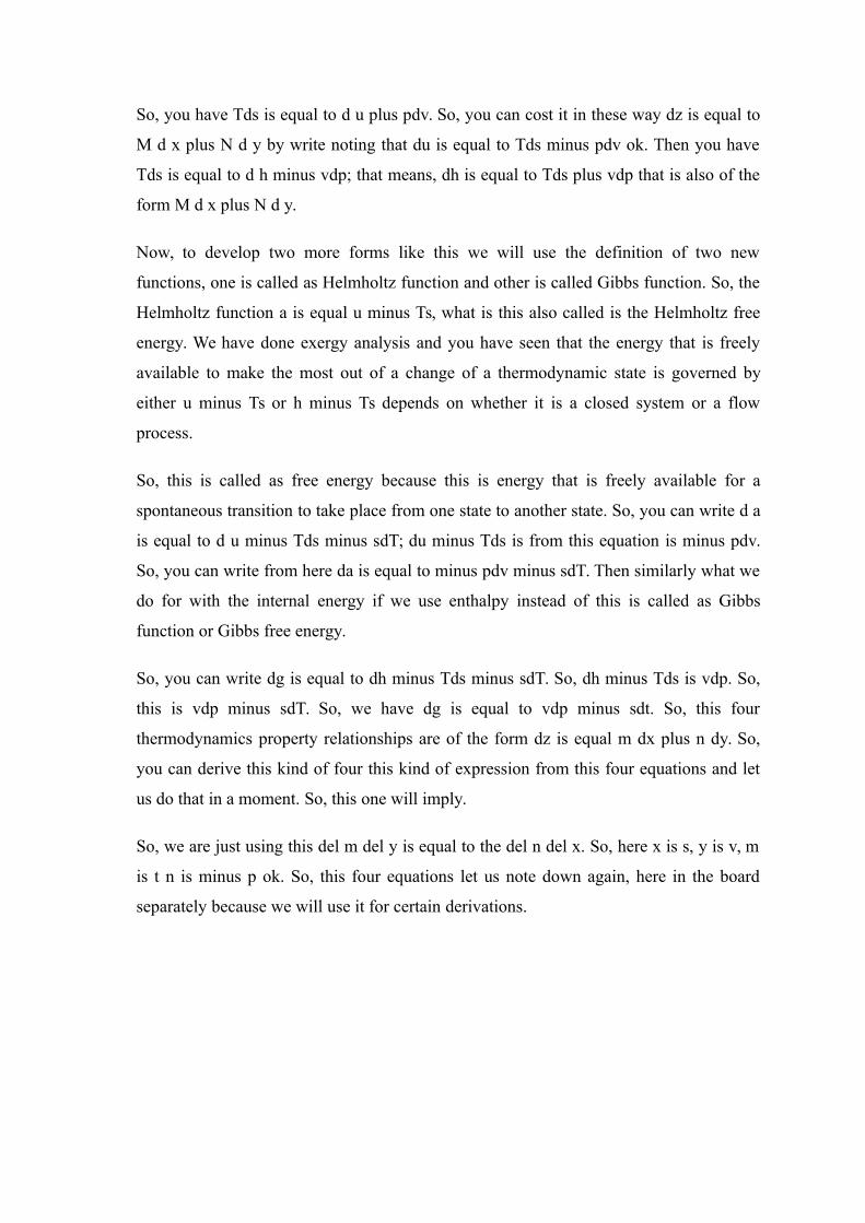
These are called as Maxwell’s relationship. These were originally introduced by

Maxwell, look at the genius of Maxwell, the same Maxwell introduced the four laws or

four rules of electromagnetism and those are Maxwell’s equations in electromagnetics.

So, you have four Maxwell’s equations in electromagnetics and here you have Maxwell’s

equation.

Student: In the third equation minus (Refer Time: 19:28).

This is not there. So, and here you have four Maxwell’s equations relationships these are

not actually called as Maxwell’s equation, sometimes this are called as called as

Maxwell’s relationships in thermodynamics. So, these are, but we will call it Maxwell’s

equation because this are essentially equations. Now in the Maxwell’s equation you can

see certain things you know very striking in Maxwell’s equation see that crosswise it is

always T and s and on the other side cross wise it is cross wise it is always p and v so T s

p v, T s p v, p v T s, p v T s. So, its you know sometimes although memorization is not

you know very important thing for understanding our particular subject, but in case you

want to you know sensitize your memory a little bit on keeping this in purview this

crosswise T s and p v can help you to some extent.

Now, you can see that these equations are very unique because this give certain

derivatives with respect to some non measurable properties like entropy in terms of

derivatives which are measurable. So, I will give you an illustration of how we can make

use of this properties by using the third Maxwell relation.

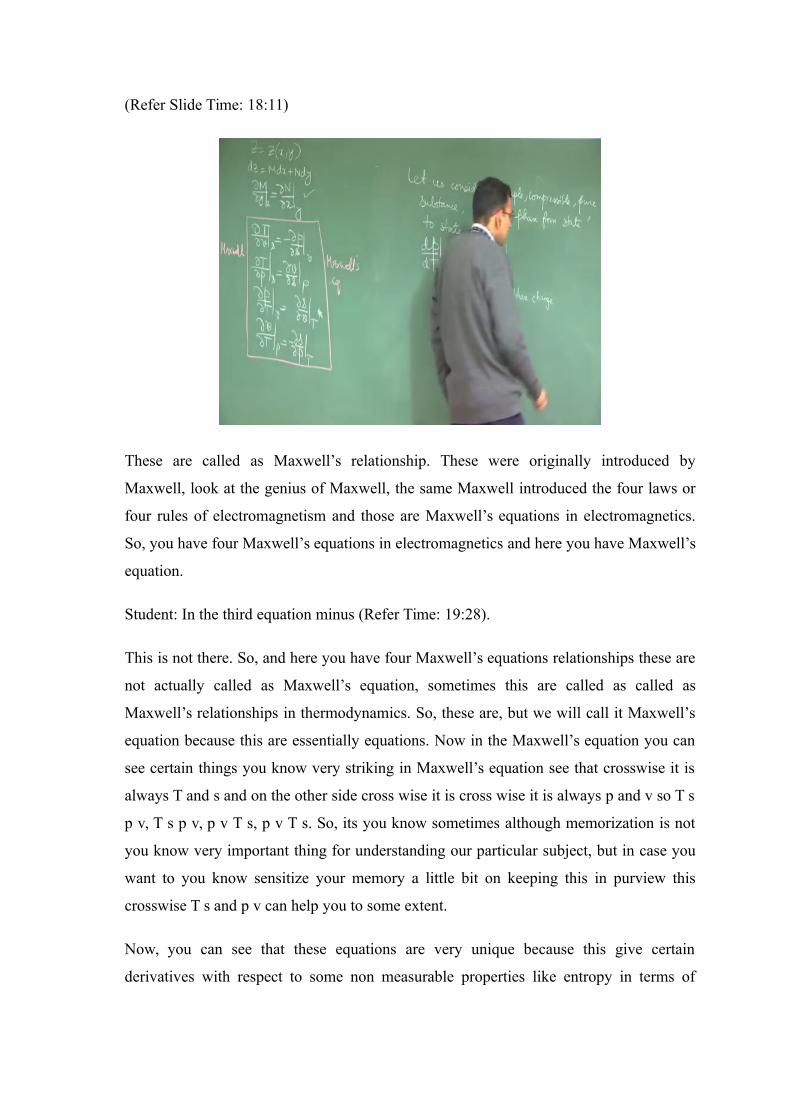
So, let us consider a phase change process of a simple compressible pure substance. So,

all these are valid for simple compressible pure substance, because then only two

independent properties are describing a state. So, the fundamental premises with which

we started our discussion is that two independent properties are describing the state. So,

it is a simple compressible pure substance. So, that is already assumed for all the

discussions that we are making today.

So, let us consider simple compressible pure substance changing phase from state prime

two state double prime ok. So, if that be the case you can write from this third T dl third

Maxwell’s equation, now if there is a change in pressure change in phase p is only a

function of T. So, this partial derivative becomes ordinary derivative and whether volume

is fixed or not is not important because p phase change is a unique function of T phase

change. So, this becomes dp dT during the phase change process.

So, this so during the phase change process the change of this is nothing, but the change

in entropy divided by the change in volume; so during phase change. Now as I have

mentioned that we will try to express the non measurable parameters in terms of

measurable parameters, entropy is not directly measurable, but we can write we can use

the Tds relation Tds is equal to dh minus vdp.

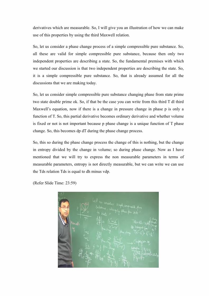
(Refer Slide Time: 23:59)

During the phase change pressure does not change right and temperature is constant. So,

0 during phase change. So, if you now integrate this from state prime to double prime,

then the temperature is fixed. So, T into s double prime minus s prime is equal to h

double prime minus h prime. So, dp dT phase change in place of this ok. So, this why

this is important because from the enthalpy of phase change which is also sometimes

called as latent heat, it is possible and from the temperature of the phase change and

volume change it is possible to get the saturation pressure versus saturation temperature

diagram.

Remember now we had a diagram for water something like this. So, saturation the phase

change pressure versus phase change temperature, this is the triple point. So, you have

solid, liquid and vapor. So, interestingly this is for water, this line has a negative slope,

can you explain through this? Imagine that the state prime is solid and the state double

prime is liquid. So, when water at a particular temperature gets converted from liquid

solid to liquid. So, its volume what happens? Its volume shrinks right, this is very typical

to water no for not all fluids this happen.

So, this is negative, T is absolute temperature it is positive and for melting this is latent

heat of melting, this is positive. So, positive divided by positive this is negative. So, that

makes dp dT phase change for solid to liquid negative right. So, you can see that this

kind of unit behaviour which we have earlier seen in properties of pure substances can be

explained by this thing.

Now, as a second example let us apply it to. So, this equation is known as Clapeyron

equation. Now let us apply it to a specific example of liquid to vapor f to g phase change

saturated liquid to saturated vapor. So, then dp dT saturated is equal to h g minus h f is

equal to hg minus h f by T into v g minus v f right. So, h fg by T into v g minus v f.

Now, we make two very important assumptions; what are the assumptions? These are

very practical, number 1 v f is much much less than vg. This is true because the density

of saturated liquid is much much more than the density of saturated vapor. So, the

specific volume is much less than that of specific volume of saturated vapor right and the

state 2 can be approximated as an ideal gas. So, state g is approximately ideal gas it is

almost full it is almost superheated vapor. So, it can be approximated as ideal gas without

bad approximation provided the pressure is sufficiently low or temperature is sufficiently

high.

If it is the other way that in operation is quite high and temperature is quite low, that will

not that combination will not normally be there then that this approximation does not

work. So, this being very close to super heated region address ideal gas approximation is

not bad. So, you can write P into v g is approximately equal to RT, R of vapor. So, this is

water vapor. So, this P is P sat.

So, then you can write here as dp dT set is equal to a h fg by T in place of vg minus v f it

is v g approximately and that is R T by P. So, then we have just one more step.

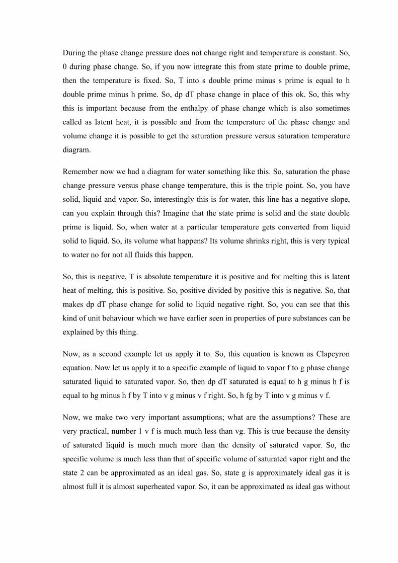
(Refer Slide Time: 30:05)

So, you can combine this two and write d of lnp dT saturation process is equal to h fg by

RT square. This 1 by P d p by p is observed in d of lnp. So, d of lnp dT is hfg by RT

square. This helps you to construct the saturation pressure versus saturation temperature

diagram for water if you know h fg at a given temperature. So, if you know the latent

heat at a given temperature, latent heat of evaporation from that data you can you can

construct the saturation pressure versus saturation temperature.

So, this is a very important relationship this is called as Clasius clapeyron equation;

Clasius clapeyron equation. So, we will consider more of these thermodynamics

relationships in the next lecture for the time being.

Thank you very much.