Concept and Implementation of a Jitter-Robustness...

FAKULTAT FUR INFORMATIKDER TECHNISCHEN UNIVERSITAT MUNCHEN

Bachelorarbeit in Informatik

Concept and Implementation of aJitter-Robustness-Analysis of Software for

Reactive Embedded Systems

Vlad Popa

FAKULTAT FUR INFORMATIKDER TECHNISCHEN UNIVERSITAT MUNCHEN

Bachelorarbeit in Informatik

Concept and Implementation of aJitter-Robustness-Analysis of Software for Reactive

Embedded Systems

Konzeption und Implementierung einerJitter-Robustheits-Analyse von Software fur reaktive

eingebettete Systeme

Author: Vlad PopaSupervisor: Prof. Dr. Dr. h.c. Manfred BroyAdvisors: Wolfgang Schwitzer,

Martin FeilkasDate: June 15, 2011

Disclaimer

Ich versichere, dass ich diese Bachelorarbeit selbstandig verfasst und nur die angegebenenQuellen und Hilfsmittel verwendet habe.

I assure the single handed composition of this bachelor’s thesis only supported by declaredresources.

Munchen, den 15. Juni Vlad Popa

Abstract

Jitter-robustness is a property of distributed embedded systems whichcommunicate through buses. The interaction between the embedded controlunits can be disturbed by jitter. In this thesis, we do not try to eliminatethe jitter sources from a technical point of view. Analysis and improvementtechniques are presented in order to make the system robust against jitter. TheFOCUS theory together with its delay calculus allow for the formal descriptionof these methods. Furthermore, AutoFOCUS 3 is the main tool in which thejitter-robustness analysis and improvement procedures are implemented andtested. A proof of concept on embedded hardware and the case study of theDENTUM Adaptive Cruise Control systems show the practical results whichcan be achieved by applying the presented methods.

Contents

1 Introduction 71.1 Motivation . . . . . . . . . . . . . . . . . . . . . . . . . . . . . . . . . . . . . . 71.2 Problem Statement . . . . . . . . . . . . . . . . . . . . . . . . . . . . . . . . . 71.3 Goals and Contributions of this Thesis . . . . . . . . . . . . . . . . . . . . . . 81.4 Overview . . . . . . . . . . . . . . . . . . . . . . . . . . . . . . . . . . . . . . . 9

2 Related Work and Concepts 102.1 Model-Based Software Development . . . . . . . . . . . . . . . . . . . . . . . 102.2 Theoretical Foundation . . . . . . . . . . . . . . . . . . . . . . . . . . . . . . . 12

2.2.1 FOCUS and Stream-Processing Functions. . . . . . . . . . . . . . . . . 122.2.2 Delay Calculus . . . . . . . . . . . . . . . . . . . . . . . . . . . . . . . 142.2.3 Causality, Delays and Buffers . . . . . . . . . . . . . . . . . . . . . . . 142.2.4 Iterative Data Flow . . . . . . . . . . . . . . . . . . . . . . . . . . . . . 152.2.5 Retiming-Transformation . . . . . . . . . . . . . . . . . . . . . . . . . 16

2.3 Introduction to AutoFOCUS 3 . . . . . . . . . . . . . . . . . . . . . . . . . . . 172.3.1 Logical Architecture, Causal Components and Delays . . . . . . . . . 202.3.2 Technical Architecture . . . . . . . . . . . . . . . . . . . . . . . . . . . 212.3.3 Deployment . . . . . . . . . . . . . . . . . . . . . . . . . . . . . . . . . 22

3 Jitter-Robustness in Reactive Embedded Systems 233.1 Defining the Term Jitter-Robustness . . . . . . . . . . . . . . . . . . . . . . . 233.2 Analyzing Jitter-Robustness . . . . . . . . . . . . . . . . . . . . . . . . . . . . 243.3 Retiming-Transformation in a Logical Architecture . . . . . . . . . . . . . . . 263.4 Improving the Jitter-Robustness . . . . . . . . . . . . . . . . . . . . . . . . . . 29

3.4.1 Reasons to Improve the Jitter-Robustness . . . . . . . . . . . . . . . . 293.4.2 Improving Basic Scenarios . . . . . . . . . . . . . . . . . . . . . . . . . 293.4.3 Optimizing the Jitter-Robustness . . . . . . . . . . . . . . . . . . . . . 31

4 Implementation of the Analysis and Transformation Methods in AutoFOCUS 3 364.1 Showing the Guaranteed Delays in AutoFOCUS 3 . . . . . . . . . . . . . . . 36

4.1.1 Motivation . . . . . . . . . . . . . . . . . . . . . . . . . . . . . . . . . . 364.1.2 Implementation . . . . . . . . . . . . . . . . . . . . . . . . . . . . . . . 364.1.3 Results . . . . . . . . . . . . . . . . . . . . . . . . . . . . . . . . . . . . 37

4.2 Extending the Causality . . . . . . . . . . . . . . . . . . . . . . . . . . . . . . 384.2.1 Motivation . . . . . . . . . . . . . . . . . . . . . . . . . . . . . . . . . . 384.2.2 Implementation . . . . . . . . . . . . . . . . . . . . . . . . . . . . . . . 384.2.3 Results . . . . . . . . . . . . . . . . . . . . . . . . . . . . . . . . . . . . 39

4.3 Implementing the Retiming-Transformation . . . . . . . . . . . . . . . . . . . 404.3.1 Motivation . . . . . . . . . . . . . . . . . . . . . . . . . . . . . . . . . . 404.3.2 Implementation . . . . . . . . . . . . . . . . . . . . . . . . . . . . . . . 404.3.3 Results . . . . . . . . . . . . . . . . . . . . . . . . . . . . . . . . . . . . 41

5

4.4 Adapting the Code Generator . . . . . . . . . . . . . . . . . . . . . . . . . . . 424.4.1 Motivation . . . . . . . . . . . . . . . . . . . . . . . . . . . . . . . . . . 424.4.2 Implementation . . . . . . . . . . . . . . . . . . . . . . . . . . . . . . . 424.4.3 Results . . . . . . . . . . . . . . . . . . . . . . . . . . . . . . . . . . . . 43

4.5 Jitter-Robustness Optimization Implemented in AutoFOCUS 3 . . . . . . . . 434.5.1 Motivation . . . . . . . . . . . . . . . . . . . . . . . . . . . . . . . . . . 434.5.2 Implementation . . . . . . . . . . . . . . . . . . . . . . . . . . . . . . . 434.5.3 Results . . . . . . . . . . . . . . . . . . . . . . . . . . . . . . . . . . . . 43

5 Evaluation 445.1 Proof of Concept on Embedded Hardware . . . . . . . . . . . . . . . . . . . . 44

5.1.1 Motivation . . . . . . . . . . . . . . . . . . . . . . . . . . . . . . . . . . 445.1.2 Setup . . . . . . . . . . . . . . . . . . . . . . . . . . . . . . . . . . . . . 445.1.3 Analysis and Transformation . . . . . . . . . . . . . . . . . . . . . . . 465.1.4 Results . . . . . . . . . . . . . . . . . . . . . . . . . . . . . . . . . . . . 465.1.5 Discussion . . . . . . . . . . . . . . . . . . . . . . . . . . . . . . . . . . 46

5.2 The Adaptive Cruise Control Case Study . . . . . . . . . . . . . . . . . . . . 475.2.1 Motivation . . . . . . . . . . . . . . . . . . . . . . . . . . . . . . . . . . 475.2.2 The ACC Functionality and Architecture . . . . . . . . . . . . . . . . 475.2.3 Possible Results of the Jitter-Robustness Optimization . . . . . . . . 495.2.4 Discussion . . . . . . . . . . . . . . . . . . . . . . . . . . . . . . . . . . 50

6 Discussion 52

7 Conclusion and Future Work 54

List of Figures 56

List of Tables 57

References 58

6

1 Introduction

1.1 Motivation

Embedded software systems are present in the daily life as part of mobile phones, cars orairplanes. These systems are mostly reactive. There is a permanent interaction between thesystem and its environment. Sensors read the environment inputs, which are processedand sent as outputs to the actuators. It is very hard to realize the software with only oneembedded control unit (ECU). In a car there would be a cabling problem for reaching allsensors and actuators from a single processing unit. This is why the embedded softwaresystem is distributed among multiple processors, which are linked through bus systems.Because of different reasons like conflicts on the MAC-layer, the expected transfer time onbus systems can be affected. The deviation from this expected transfer time is called Jitter.If this jitter is not treated properly, it can damage the correctness of the system outputs.

Contribution of this thesis. Metaphorically speaking, the jitter-robustness is like anairbag to the system, which improves the degree of tolerated deviation in transmissiontime. From the software developers perspective a new design approach is introduced.After designing the new system, the developer has the possibility to analyze its jitter-robustness and finally improve it on demand. All the jitter-robustness analysis andimprovement techniques can be done statically before runtime. For example, somesoftware systems in the automotive industry like the ABS (Anti-Blocking-System) shouldbe as jitter-robust as possible. In this case a system failure could have consequences for thedriver.

1.2 Problem Statement

In this thesis we purpose an analysis of the jitter-robustness of a system regarding itslogical and technical architecture together with their deployment mapping (see figure 1).With transformation methods like the retiming-transformation (see section 2.2.5) we try toimprove the systems robustness against jitter.

Considered aspects. The analysis is formulated on the structural level of the logicalarchitecture. This means, in this thesis the behavior of the components is not taken intoaccount.

Figure 1 shows a logical architecture containing three components: C1, C2, C3 commu-nicating through channels: m1, m2 and a technical architecture with two CPU’s whichexchange information through a bus. The deployment mapping assigns the componentsC1, C2 to the first CPU, while the component C3 runs independently on the second CPU.C1 sends inside the first CPU a message to C2 which communicates with C3 through thebus. Channel m2 is mapped on the bus and is responsible for this communication. This is

7

C1 C2 C3 m1 m2

Logical Architecture

Technical Architecture

C1 C2 C3

m1

m2 Bus

CPU1 CPU2

Deployment

Deployment

CPU internal communication for channel m1 Possible jitter on bus for channel m2

Figure 1: A logical architecture deployed on a technical architecture.

an example of a possible scenario where jitter can affect the inter-processor communication(IPC) between two software components (C2, C3).

1.3 Goals and Contributions of this Thesis

The main goals are to analyze and improve the jitter-robustness of the software for reactiveembedded systems. Furthermore, the presented techniques are evaluated with the casetool AutoFOCUS 3. For evaluation we use the DENTUM Adaptive Cruise Control modelfrom the automotive area as a basis.

The major contribution of this thesis is the description of a linear program-ming based jitter-robustness optimization method.

In this thesis the following topics are covered:

1. Conception of an analysis method, which will determine for each component of amodel its robustness to jitter.

• Deployment of a logical architecture on a technical architecture is known.

• This method returns the jitter-robustness in logical ticks of the system.

2. Develop a concept for improving the jitter-robustness.

• This concept can change the causality of the logical architecture but theinput/output behavior of the deployed system has to stay the same.

• A relevant transformation technique, which works on data flow graphs is calledretiming-transformation. A detailed description of this can be found in [LS91].

• The improvement is constrained to the structural level.

8

3. Prototypical implementation of these concepts in AutoFOCUS 3.

• AutoFOCUS 3 should support causality with arbitrary order.

• The retiming-transformation has to be adapted to the logical architecture ofAutoFOCUS 3.

4. Evaluation of the concepts with case examples.

Given a logical model and its deployment, the reader should be able to calculate its jitter-robustness in abstract time units (ticks) and should know the possibilities how to improveit.

1.4 Overview

This thesis consists of several sections which are structured as follows. The 2. sectionprovides the background of concepts from related work which is often used. The maindevelopment artifact is the model-based development (see section 2.1). This methodologyis implemented in the case tool AutoFOCUS 3 which is presented in section 2.3. The jitter-robustness analysis relies on the FOCUS theory with its delay calculus which is brieflydescribed in section 2.2. Section 3 presents some methods used to analyze and improvethe jitter-robustness of the system. In order to make this methods in AutoFOCUS 3possible,the following section 4 extends the functionality of this tool. Afterwards, section 5 presentsa proof of concept on embedded hardware and the results of the practical case example, theDENTUM Adaptive Cruise Control model, from the automotive industry. Furthermore,a discussion section 6 clarifies some aspects in this thesis and the concluding section 7describes new paths and approaches on how new methods can be developed in futurework.

9

2 Related Work and Concepts

This section covers the explanation of the concepts used in this thesis. It contains adescription of model-based development, followed by the presentation of the FOCUS

theory and the iterative data flow graphs. In section 3 we use the FOCUS delay calculustheory as a concept for analyzing the jitter-robustness. Nevertheless, a brief introductioninto AutoFOCUS 3 presents the features of the case tool used in this thesis.

2.1 Model-Based Software Development

Models, metamodels and meta-metamodels. Nowadays, there are complex embed-ded software systems which react on inputs by producing outputs. Most of the timesthese systems are distributed and can not be generally realized with only one embeddedcontrol unit (ECU). The model-based development is adequate for this kind of systemsbecause it aims to reduce the development complexity with the help of abstraction. In

Figure 2: The model, metamodel and meta-metamodel of a state diagram.

this context it is very common to define the meta-metamodel, the metamodel and themodel. These three layers of abstraction should be sufficient for describing the system.The model is a instantiation of a metamodel, which in turn is a instantiation of a meta-metamodel (see figure 2). Textual or graphical representation of the system defines amodel. For example, if the model is a state diagram, the metamodel represents the artifacts

10

used for creating the model and their relationships. In this case the metamodel containsstates and transitions. Each state can contain other states and can have any number ofingoing/outgoing transitions. The transitions exist between two states. Therefore, themeta-metamodel includes the associations and metamodel-classes used in the metamodel.More information to this is found on the OMG-Websites at the MOF-standard [MOF].

Granularity levels and perspectives. As shown in Figure 3, the amount of detail isreduced and abstraction is achieved by:

• Decomposition of the systems into its sub-systems, which have a lower level ofgranularity. The sub-systems which do not contain other sub-systems are called basicblocks.

• Consider different development perspectives like: requirements perspective, func-tional perspective, logical perspective, technical perspective. More details are foundhere [TRS+10].

Requirements Perspective Functional Perspective Logical Perspective Technical Perspective

Entire System

Level of Granularity

…

Supersystems

Systems

Subsystems

…

Basic Blocks

Software Engineering Perspectives

FSys

…

… …

CSys

C1

…

…

ECU

coarse

fine

F1 Fn

FA FB

FC

C2

C3

C11

C3m

ECU Sens

Act

RSys

…

…

Figure 3: Different granularity levels (vertical) and different software developmentperspectives (horizontal) according to [TRS+10].

The main challenge with model driven development is the mapping of models fromdifferent perspectives. Models with the same level of granularity have to be mappedtogether (horizontal allocation) and attached to their sub-systems (vertical allocation). A com-prehensive modeling theory which can solve this challenges by creating a mathematical

11

model is called FOCUS theory [RST09]. A case tool which is based on this theory is calledAutoFOCUS 3[Aut].

Figure 3 shows the different granularity levels on the vertical axis and the software per-spectives on the horizontal axis. In the requirements perspective timing and performanceconstraints can be set. These determine the end-to-end latency which influences the jitter-robustness. The functional perspective is used to describe the system behavior. In thisthesis, the jitter-robustness is analyzed regarding the logical and technical perspective.The three marked rectangles in the bottom right corner of figure 3 show the granularitylevels of the perspectives which are relevant for the jitter-robustness in this thesis.

2.2 Theoretical Foundation

In this section, a fundamental way of describing systems called FOCUS is introduced.With the help of stream-processing functions, this theory efficiently describes systems ofcomponents, which process a specific function.

2.2.1 FOCUS and Stream-Processing Functions.

A stream is a finite or infinite ordered sequence of elements. Let M be a set of messages.We use the following notation:

• M∗: contains all finite sequences over M including the empty sequence <>.

• M∞: contains all infinite sequences over M .

• Mω: contains all sequences over M (Mω =M∗ ∪M∞).

For the channel histories it is useful to consider the timed streams: (M∗)∞ which consist ofa infinite stream of finite sequences. For each time t ∈ N (in ticks) the element on position tof the timed stream represents the finite sequence that is being sent on the channel in thattick. To operate with timed streams, some functions are being introduced in [BS01] and[Bro10]:

• x.t gets the t-th element of the stream x.

• #x gets the number of elements the stream x contains.

• xay concatenates the two streams.

• x ↓ t gets the prefix of length t of x. If: t ≥ #x⇒ x is returned.

• Ssx returns a stream from x by filtering only the elements contained in S.

• x v y ≡ ∃z : xaz = y.

• x returns the sequence by concatenating all the elements of the timed stream x.

12

For specifying the functionality of a system, FOCUS uses schemes as presented in table 1.The first row provides a black-box view of the analyzed component. Each input/outputchannel is associated with a specific data type (or set of messages). The second row is usedto describe from a glass-box view the functionality of the component. One can apply herethe stream-processing functions presented above.

<name>in <input channels>out <output channels><expression>

Table 1: FOCUS specification of a system.

Figure 4 and the first row of the FOCUS specification table 1 illustrate the syntacticalinterface of a component. This representation does not give details about the causality ofa system. It only defines its structural level. For each component a set of input and outputchannels express how many messages are being processed and returned. This provides ablack-box perspective of the system which is important for the jitter-robustness analysisand improvement in this thesis.

Example 2.2.1. Let there be two sets A and B which both contain a third set C. In otherwords, the following holds: A = C ∪X1 and B = C ∪X2, where X1 and X2 are subsets ofC and |X1|, |X2| < C. Furthermore, we want to build a component F with a syntacticinterface like the one seen in Figure 4. F is responsible for filtering from both input

B Filter Function

F

A B

C

Figure 4: The filtering function which has two inputs from the sets A and B and filters outthe messages which belong to the set C.

13

channels of type A and B the messages contained in C. Using the FOCUS notation, thescheme 2 provides all the semantic and syntactic information needed for the specificationof the component F .

F

in x : A, y : B

out z : C

z = C s xaC s y

Table 2: FOCUS specification of component F .

2.2.2 Delay Calculus

Guaranteed Delays and Delay Profiles For the delay calculus we use terms such asguaranteed delays or delay profiles. In a network of components there can be many pathsfrom arbitrary inputs that lead to the same output channel. For a output channel o theguaranteed delay is equal to the minimum sum of delays on each of the paths that leadto this channel. We use the following notation for the guaranteed delays: gardelay(F, o),where F is the component and o is an output channel of F . Consequently, let there be F ′,the same system as F , with only the one input channel i. The delay profile is defined as amapping that contains for each output channel o and each input channel i the guaranteeddelay of o in the new system F ′.

A profound introduction and definition of the delay calculus is described by Broy in[Bro10]. This work is also pointing the way for the analysis presented in this thesis.

2.2.3 Causality, Delays and Buffers

In this thesis the terms causality, delays and buffers are frequently used. It is essential tounderstand the context in which these words are used because they all share similarities.The term causality is associated with components, which can be either strongly or weaklycausal. Furthermore, all strongly causal components are supposed to delay the inputs bya positive and nonzero number of time units.

Implementation of delays Delays are typically implemented by FIFO-buffers. A delayof x time units can be simulated by a first-in-first-out (FIFO) buffer of size x. Assuming thatthe pop- and push-method are being called once in every tick and that the buffer containsexactly x elements, then the popped elements have to be x ticks old. This method for theimplementation of the delays has a certain amount of flexibility. If the messages are beingreceived to slow (because of jitter) then the user, perceiving the system from the outside,will not notice a difference on the behavior until one of the buffers is empty. Therefore,such a principle for the delays implementation and consequently for the realization ofcausality can have a big impact on the robustness of the system.

14

2.2.4 Iterative Data Flow

According to [Par89, DK82, Ack82, Den80], the data flow representation of a algorithmis appropriate for expressing the available concurrency in a multiprocessor environmentsuitable for distributed embedded systems. The data flow language is presented in W.B.Ackerman’s article [Ack82]. Furthermore, general concepts of modeling systems with dataflow program graphs are found in [DK82]. The iterative data flow model is used forthose models which have a global clock. The functionality of these models is executedin each tick. In this thesis, the data flow programs, represented by data flow graphs, aresynchronous and nonterminating.

Figure 5: The data flow program and data flow graph.

Data flow programs and graphs. Figure 5 shows how a data flow program (a) istranslated into a data flow graph (b). The data flow program computes in each time unit tthe expression x(t)× 3 + y(t)× 2 and assigns it to z(t). The equivalent data flow graph isshown in (b). Data flow graphs are acyclic graphs containing environment inputs/outputs,vertices (tasks), edges (channels) and delays on edges. Environment interface points arerepresented by the dashed circles. Delay units appear in rectangles with the value ’D’.They have the role to slow down the transmission by one time unit. Note, that there maybe edges which do not contain any delay units. The vertices A, B and C of figure 5(b) aretasks executed in each step. These tasks describe functions of arbitrary arity that receiven ≥ 0 inputs and produce m ≥ 0 outputs. Hence, inputs x(t) and y(t) are multiplied by 3

respectively 2, added together and sent as the result z(t+ 1).

Delay operators. Sometimes, outputs need to be delayed by several time units beforethey are received. Therefore, the data flow graphs allow delay units to be specified foreach channel. If a channel from node A to node B contains i delays, B gets the message Asent at time unit t− i (for all t > i). Notice that for those ticks in which t ≤ i, initial valueshave to be specified.

15

Homogeneous and heterogeneous data flow graphs. In this thesis, a homogeneousdata flow graph is a graph in which all outgoing channels of a vertex have the samenumber of delays assigned. This definition introduces the term causality for data flowgraphs. In a homogeneous graph the vertices which do not have any delays on theoutgoing channels are called weakly causal. All other vertices are strongly causal. Theheterogeneous data flow graphs are those graphs which accept outgoing channels withdifferent delay numbers.

2.2.5 Retiming-Transformation

The retiming-transformation is a method for changing data flow graphs so that the end-to-end latency remains the same. Therefore, the system behavior remains the same on theoutside. Retiming was first introduced by Charles E. Leiserson and James B. Saxe in [LS91]as a transformation method for synchronous circuitry. Initially, this transformation wasused to reduce the minimal clock period and to improve the performance of the systems.In this thesis, the retiming-transformation will be adapted to the logical architecture ofAutoFOCUS 3 (see section 3.3) in order to improve the jitter-robustness by shifting delaysin the network.

The technique uses a data flow graph G(V,E, δ), where each vertex in V can execute afunction and edges in E can contain a non-negative number of delays determined by thefunction δ : E → N. Therefore, the following must be valid:

∀e ∈ E,∃n ∈ N : n ≥ 0 ∧ δ(e) = n

This means, each edge gets assigned a positive number of delays. The retiming-transformation can be described with the help of the function r : V → N, with the property:

∀v ∈ V,∀e = (u, v) ∈ E : r(v) ≤ δ(e)

This means, the retiming-transformation is a number smaller or equal to the number ofdelays on all incoming edges. The new transformed graph Gr has the same set of verticesV and edges E but a different delay function δr. The values of this function are:

∀e = (u, v) ∈ E : δr(e) = δ(e) + r(v)− r(u)

The retiming-transformation takes for each vertex v, r(v) delay units from all inputs andadds them to all the output channels (Analog, retiming can also be done by moving thedelays from the output channels to the input channels). Furthermore, the following twolemmas take place (proof can be found in [LS91]):

Lemma 2.2.1. For every path P from u to v we have δr(P ) = δ(P ) + r(v) − r(u), whereδ(P ) represents the number of delays on P .

Lemma 2.2.2. The number of delays on every cycle will not be modified.

16

B

A A’

x+y1 D

x+yn D

x+z1 D

x+zm D

z1 D

zm D

y1 D

yn D

Figure 6: The two possible retiming-transformations that can be executed on a component.Delays can either be moved from inputs to outputs or vice versa.

Retiming-transformation as a linear problem. In the late 80’s C.E. Leiserson and J.B.Saxe used the retiming-transformation to minimize the clock period. The algorithm whichspecifies how to retime the system is described in [LS91]. It transforms this problem into alinear problem by computing a system of inequalities of the forms:

r(x)− r(y) ≤ Wxy − 1 (1)

r(x)− r(y) ≤ δ(e) (2)

which then has to be solved. r(x) and r(y) stand for the retiming-transformation numberof the two nodes x and y. For inequality 1, Wxy represents the number of delays on the lessdelayed path between x and y. If there is a edge e between x and y the inequality 2 comesinstead. This is a difference-inequality system which can be solved by linear programmingtools like lp solve [Lp] or SMT-solvers like Z3 [Res]. In section 3.4.3 the optimization of thejitter-robustness with help of the retiming-transformation is presented as a linear problemwhich is efficiently solved by the tool lp solve.

2.3 Introduction to AutoFOCUS 3

The scientific case tool AutoFOCUS 3 implements major parts of the FOCUS theory, whichallows model-based development. It has a graphical view to model the system by ’clicking’components and channels. Initially, the AutoFOCUS 3 development was motivated by thelack of a case tool which does not concentrate exclusively on aspects like code-generationand user interface, or is too mathematical oriented for the system engineer [HS01]. This

17

section provides a brief introduction to the main features of AutoFOCUS 3.

Timing model in AutoFOCUS 3. In FOCUS theory systems consist of componentswhich communicate with each other through communication channels [BS01]. Besidesexplaining the causality between the components which determine a specific data flow,this thesis will have to deal with problems caused by the transition from the real time,represented by real numbers, to the discrete time which will only contain discrete intervals.Discrete time advances in ticks, where two events within a tick will not be differentiated.In the context of this thesis, we use the same timing model as presented in [HHR09]. Thismeans, in AutoFOCUS 3 we assume there is a global clock responsible for the synchronicityof time. Also, we assume that the time model is discrete and advances in ticks, so thatevents within a single tick can not be distinguished. This is a difference to the FOCUS

theory, where events are asynchronous.

AutoFOCUS 3 consists of several graphical views which show different perspectives ofthe system under design, comparable to the perspectives in figure 3.

System structure specification. This specification shows a static view of the describedsystem. It can be seen on the left side of the figure 7. According to [BFG+08], the elementsof the system structure specification are:

• Ports let components communicate with the environment via channels. Each porthas a data type and a name and is either an input port or an output port. An inputport can only have one ingoing channel. An output port can connect to multipleoutgoing channels.

• Channels realize the directed communication between components, binding themthrough their ports. They also have names and data types which have to becompatible with the ones from the involved ports. The logical architecture ofAutoFOCUS 3 contains only directed channels. This means that the flow of messagesgoes in one direction (from the output port to the input port).

• Logical components can communicate with each other through channels, form-ing a network. They are entities containing interface, structural and behavioralinformation. Furthermore, the system structure specification can also be seenfrom a hierarchical point of view, where each component may have its own sub-components (observe similarities to model-based development in section 2.1). Eachcomponent communicates with the environment through its parent-component. Allcomponents have a syntactic interface, determined by their input and output ports,creating a black-box view of their functionality. The semantic interface containsbehavior specifications like: stateful automaton specifications or stateless functionspecifications. This interface can be observed at the level of the atomic components,which can no longer be divided in sub-components. In the current implementation

18

of AutoFOCUS 3, components are weakly or strongly causal. Weakly causal meansthe outputs are sent within the same tick to the next component or environment. ForStrongly causal components the outputs are delayed by exactly one logical tick. Animportant constraint, is that weakly causal cycles are not allowed.

Automaton specification. This specification is part of the component behavior view andcan be seen on the right side of figure 7. It consists of an automaton with control states, datavariables, transitions, inputs and outputs. Among all control states there is an initial state,and all data state variables have to have a initial value [HST10]. Every transition is boundto a source and a destination state. It must contain an input pattern, preconditions, anoutput pattern and optionally postconditions. The input patterns check if the input portshave the desired values. Preconditions define a pattern containing data state variables andinput ports which has to be true. The output pattern assigns new values to the outputports. Postconditions assign values to data state variables. Further clarifications to thesyntax and semantic of the transition specification can be found in [Aut].

Figure 7: AutoFOCUS 3 structural and automaton view. In the structural specificationview the PCS system is a atomic component, whose behavior is shown by theautomaton on the right side. The input ports are represented by white circlesand the output ports are shown as black circles.

19

2.3.1 Logical Architecture, Causal Components and Delays

The logical architecture contains information about the system structure and its behavior.The basic principle is to split the system into its suitable sub-systems, which communicatethrough channels and also form a hierarchical view. On the leaf level, sub-systems containbehavioral information. The main aims of the logical architecture are to:

• structure the system into communicating logical components.

• easily integrate existing components and increase reusability.

• make a seamless transition to the technical architecture.

Delays and causality in AutoFOCUS 3 For AutoFOCUS 3 the term causality is usedto express the amount of delays on the outputs of the components. In the currentimplementation, a strongly causal component delays all outputs by a exactly one tick.A weakly causal component does not delay its outputs at all. If a principle such as theretiming-transformation is adapted to the AutoFOCUS 3’s logical architecture, the stronglycausal components will have to be able to delay the output by more than one time unit(see section 4.2).

Weakly and strongly causal components. As already described above, there are twocomponent types: weakly causal components and strongly causal components. Thissection contains mathematical definition of the causality of a component based on FOCUS

theory, using the notation from [BS01, Bro10]. Let F be the function defining the I/O-behavior of a given component:

F :−→I → ℘(

−→O )

This function F is called:

• weakly causal (or properly timed) if the formula: x ↓ t = z ↓ t⇒ (F.x) ↓ t = (F.z) ↓t is true;

• strongly causal (or time guarded) if the formula: x ↓ t = z ↓ t ⇒ (F.x) ↓ t + 1 =

(F.z) ↓ t+ 1 is true.

In other words, if the output at a random time t does not depend on input that is receivedafter time t, the component is weakly causal. If the output at time t does not depend onan input that is received after time t − 1, the component is strongly causal. A possibilityto create strongly causal components is to delay all their output channels by exactly onetime unit. This is how strongly causal components are implemented in AutoFOCUS 3.Therefore, a method to define the length of a logical tick can be described by assigningit length of the the critical path (the longest time consuming chain of weakly causalcomponents). If the tick is shorter, the weakly causal formula will not be valid. Notice thatthe weakly causal components must not contain any feedback loops (Brock-Ackermannanomaly see [BA81]). Otherwise, the longest chain will be infinitely long and the logicaltick will never end.

20

Delaying messages. For F a I/O-behavior describing function and n ∈ N ∪ {∞}, wedefine:

delay(F, n) ≡ [∀x, z, t : x ↓ t = z ↓ t⇒ (F.x) ↓ t+ n = (F.z) ↓ t+ n]

[Bro10]. This binary function suggests the response delaying on all output channels byn ticks. We define Fs and Fw as the I/O-behavior functions that are responsible for astrongly causal component and a weakly causal component. Therefore, delay(Fs, 1) anddelay(Fw, 0) must hold.

Weakly and strongly causal components to data flow graphs. The concept of causal-ity can also be adapted to iterative data flow graphs. Section 2.2.4 provides the theoreticalbackground for the causality in homogeneous data flow graphs. Figure 8 illustrates how

Fs

i1 i2

in

o1 o2

om

Fs

i1(t) i2(t)

in(t)

o1(t) o2(t)

om(t)

D

D

D

(a)

Fw

i1 i2

in

o1 o2

om

Fw

i1(t) i2(t)

in(t)

o1(t) o2(t)

om(t)

(b)

Figure 8: The translation of the weakly and strongly causal components to homogeneousiterative data flow graphs.[Sch11]

weakly and strongly causal components are translated to data flow graphs. The weaklycausal component Fw in figure 8(b) has the input interface Iw = {i1, . . . , in} and theoutput interface Ow = {o1, . . . , om}. There are no delay units on the output channelswhich means, the result is passed on to the next component within the same logicaltick. The values on the output channels are: o1(t) = Fw(i1(t), . . . , in(t)), . . . , om(t) =

Fw(i1(t), . . . , in(t)). Figure 8(a) sketches the translation of the strongly causal componentFs into a data flow graph. The syntactic interface of component Fs consists of theinput channels Is = {i1, . . . , in} and the output channels Os = {o1, . . . , om}. Eachoutput channel of the data flow graph vertex contains one delay unit. Hence, the outputchannel values in each time unit is: o1(t + 1) = Fw(i1(t), . . . , in(t)), . . . , om(t + 1) =

Fw(i1(t), . . . , in(t)).

2.3.2 Technical Architecture

The technical architecture describes the hardware on which the software runs (ECU’s,buses, sensors and actuators). An advantage of using a technical architecture is that the

21

hardware platform can be changed independently from the logical architecture. The aimsof the technical architecture are to:

• present an abstract view of the hardware (ECU’s, buses, sensors and actuators) andits topology.

• describe the sensors/actuators, operating system and drivers.

• ensure that the deployed system fulfills the functional and non-functional require-ments.

2.3.3 Deployment

The deployment describes the mapping of the logical components and channels to aspecific hardware platform. If two components, which communicate through a channelin the logical architecture, are deployed on different processors, then that channel has tobe mapped on a bus that binds the two processing units. Deployment is important tothe jitter-robustness. A different deployment mapping can lead to a different robustnessagainst jitter. As mentioned in section 1.2, all the methods presented in this thesis analyzeand improve the jitter-robustness for systems with a specific deployment mapping.

22

3 Jitter-Robustness in Reactive Embedded Systems

After explaining in the previous section 2 the necessary concepts, this section covers thedefinition, analysis and improvement of the jitter-robustness.

3.1 Defining the Term Jitter-Robustness

For defining the term jitter-robustness, it is necessary to understand the words jitter androbustness. Firstly, the word robustness refers to a software quality aspect. Secondly,jitter expresses the lag in time which can occur while sending a message. Embeddedcontrol units (ECU’s) communicate with each other through bus systems. Therefore, somechannels in a network of components may be mapped on buses. Sometimes messages senton bus are being received sooner or later then the expected time. The deviation from thisexpected time is called jitter (see figure 9). Regarding these definitions, jitter-robustness isthe amount of jitter, which does not affect the correctness of the outputs of a system. Theoutputs are considered correct if they are functionally correct and additionally have thecorrect timing. The aim of this thesis is to present the jitter-robustness as a metric that ismeasured in logical ticks.

(a)

Expected Arrival Time Scope of this

Bachelor Thesis Bus Driver

to early/ rate to high

to late/ rate to low

Jitter-Deviation

(b)

Figure 9: The definition of jitter and the jitter-deviation which is analyzed and handled inthis thesis.

Figure 9 shows in 9(a) two ECU’s which communicate with each other through a buswhere jitter takes place. According to figure 9(b) the jitter-robustness is analyzed andimproved for those messages that are received to late or with a low rate. If the incomingmessages are received sooner than expected, the bus driver can save the data in ring-buffers.

Technical issues that cause jitter. Some embedded systems deliver safety criticaloutputs. An output is acceptable if it is semantically correct and it is delivered in duetime. Especially these safety critical systems have to be as jitter-robust as possible.

This thesis will not try to explain from a technical point of view how to fightthe possible reasons for jitter. It will try to cope with them!

23

The important technical issues that cause jitter are the following:

• Resource conflicts/concurrency. In complex systems there are usually more thantwo partners which exchange information on the same bus. There can be simultane-ously many messages on the bus, which delay the sending of a specific message. Forexample, the CAN-bus (Controller Area Network, [Gmb]) introduces an arbitrationprinciple which always sends the package with the lowest ID. That is why messageswith higher ID have to wait all messages with lower ID’s are sent.

• Electromagnetic compatibility (EMC). Electromagnetic impulses can change the bitsof messages that are sent. When data is received, some bus systems (e.g. CAN-bus) perform a cyclic redundancy check (CRC, see [PFTV]). This method is capableto detect any error caused by the EMC and hence, a time costing resubmission isnecessary.

• Synchronization. The synchronization of all ECU’s over a longer period of time isnot trivial. Especially for those systems which have a high operating frequency, thefull synchronization over more units is very difficult. This problem is caused by thetransition from the real time which is continuous to the discrete time representationof the machines. There always is a delta of time between the ECU’s that can growover a longer period of time.

3.2 Analyzing Jitter-Robustness

In a top-down approach, the software developer designs the software, analyzes it andimproves it if necessary. A main advantage in analyzing the jitter-robustness is that it canbe done in an early phase. The purpose of this subsection is to define for a given system ifa improvement of the jitter-robustness is needed. In the scope of this thesis the analyzedmodel has to match some assumptions:

• The technical architecture of the given system contains only one bus.

• The deployment mapping of the bus divides the logical architecture into two disjointsets of components on two ECU’s.

Let there be A the super-component that contains all components from one set and B

the super-component that contains all components from the other set. Furthermore, letthere be IA and OA the sets of all input and output ports of A and IB and OB the setsof all input and output ports of B. The super-components A and B can also be seen asfunctions: A :

−→IA → ℘(

−→OA) and B :

−→IB → ℘(

−→OB). For each system the jitter-robustness

can be measured in ticks by the function ρ. Let there be IBA a subset of IA with followingdefinition:

IBA = IA ∩ {o ∈ OB|∀x ∈−→IB ⇒ (B.x).o ∈

−→IA} (3)

24

This means IBA contains all channels deployed on the bus from component B tocomponent A. If the following holds:

∀o ∈−→OB ⇒ ¬(∃x ∈

−→IB ∧ (B.x).o ∈

−→IA)

meaning that S does not contain feedback channels from A to B, then IBA = φ. Analog,let there be IAB a subset of IB with:

IAB = IB ∩ {o ∈ OA|∀x ∈−→IA ⇒ (A.x).o ∈

−→IB} (4)

For the jitter-robustness analysis we need to consider the following components:

A′ :−−→IBA → ℘(

−→OA) (5)

B′ :−−→IAB → ℘(

−→OB) (6)

Note that these new components have the same functionality as A and B restricted on thenew input ports. Therefore, the jitter-robustness it equal to:

ρ(S) = min{min{gardelay(B′, o)|∀o ∈−→OB},min{gardelay(A′, o)|∀o ∈

−→OA}} (7)

This formula states that the jitter-robustness is equal to the number of causalities (delays)on the least delayed path from an input to an output from both components A′ and B′.

Feedback

Bus

A B

C4

C5

C1

C2

C3

Figure 10: A valid AutoFOCUS 3 model satisfying the necessary constraints for jitter-robustness analysis in this thesis. C1, C2 and C3 are feed-forward channels.Optionally the system may contain additional feedback channels (C4 and C5).

25

3.3 Retiming-Transformation in a Logical Architecture

As already mentioned in Section 2.2.5, the retiming-transformation is a technique formoving the delays in an data flow graph without changing the end-to-end latency.Retiming is the central technique for shifting delays in section 3.4.3. The algorithm of thistransformation takes a constant number of delays from all input channels and adds it toall output channels or vice versa. A problem with logical architectures of AutoFOCUS 3is that the corresponding data flow graph is always homogeneous. In other words,there is no surjective function which assigns for each data flow graph (homogeneousor heterogeneous) a logical architecture. Hence, the method for adapting the retiming-transformation to a logical architecture is not unique.

Adapting the retiming-transformation to the logical architecture. A logical ar-chitecture contains ports, channels and components (see Section 2.3). The retiming-transformation in a logical architecture is performed on the components. The only precon-dition necessary for the transformation to take place is that all predecessor componentsare strongly causal. Predecessor components are those components that have at least onechannel that leads to the analyzed component. This condition is equal to the one for dataflow graphs where every input channel should have at least one delay to offer (see section2.2.5). Note that a strongly causal component can contain more than one delay unit (forclarifications see section 4). Therefore, the retiming on a specific component can be donewith an integer value greater than zero and smaller than the lowest causality order ofall predecessor components. To express everything in mathematical terms, let there be Cthe set of all components of a system. We define the function δ : C → N representingfor each component the causality order it has. Hence, δ(X) = 0 means component Xis weakly causal. Furthermore, let there be function π : C → P(C) which returns forevery component all its predecessors and function µ : C → P(C) which returns forevery component all its successors. The retiming-transformation is described as a functionr : C → N. For a component X with r(X) > 0 the transformation will increase the numberof delays of this component by r(X). Let there also be the function δr defined the same asδ. It represents the causality order for each component after the retiming-transformation.In order to preserve the end-to-end latency of the system r(X) causality delays on thepredecessors output channels have to be removed. Therefore, the following holds:

∀P ∈ C : δr(P ) = δ(P )−U∑

µ(P )

r(U) + r(P ) (8)

However, a problem still persists. For those paths from a component P ∈ π(X) that leadto an output and do not have X in it, the number of delays is with r(X) units smaller. Thisis because of equation 8. To fix this, an ID component, processing the identity function,has to be created for: ∀P ′ ∈ µ(π(X)) \ X . The ID component communicates with thepredecessor P of X and its direct successor P ′. Furthermore, ID is strongly causal and hasδr(ID) = r(X).

26

Example 3.3.1. The following figures 11, 12, 13 and 14 will show step by step how theretiming-transformation operates in a logical architecture.

A

B

C

r(A) = x

δ(A) = y

δ(B) = z

r(B) = 0

r(C) = 0

δ(C) = t

δ(P2=(B,C)) = z + t

δ(P1=(B,A)) = z + y

Figure 11: The first step of the retiming-transformation in a logical architecture.

There are three strongly causal components A, B and C with their corresponding delayfunctions δ(A) = y, δ(B) = z and δ(C) = t in figure 11. Component A needs to be retimedbecause r(A) = x > 0. The first step of the retiming-transformation is to ensure that thenecessary preconditions are satisfied. Hence, r(A) = x < δ(B) must hold.

A

B

C

r(A) = x

δr(A) = x + y

δ(B) = z

r(B) = 0

r(C) = 0

δ(C) = t

δ(P2=(B,C)) = z + t

δ(P1=(B,A)) = x + y + z

Figure 12: The second step of the retiming-transformation in a logical architecture.

The second step of the retiming-transformation is to add the necessary delays to theretimed components. Therefore, component A gains x causality delay units (deltar(A) =

27

x+ y), which causes the path P1 that begins with B and ends with A to change its latency.This is signalized in figure 12 with the red color (δ(P1) = x+y+z instead of δ(P1) = z+y).

A

B

C

r(A) = x

δr(A) = x + y

δr(B) = z - x

r(B) = 0

r(C) = 0

δ(C) = t

δ(P2=(B,C)) = z - x + t

δ(P1=(B,A)) = z + y

Figure 13: The third step of the retiming-transformation in a logical architecture.

In the third step of the retiming-transformation the number of delays on P1 is adjusted.A consequence is that the path P2 between B and C looses x delay units. The number ofdelays on P2 is z − x+ t instead of z + t (see figure 13).

A

B

C

r(A) = x

δr(A) = x + y

δr(B) = z - x

r(B) = 0

r(C) = 0

δr(C) = t

δ(P2=(B,C)) = z + t

δ(P1=(B,A)) = z + y

ID δr(ID) = x

r(ID) = 0

Figure 14: The forth step of the retiming transformation in a logical architecture.

The last step of the retiming transformation is illustrated in figure 14. The end-to-endlatency of P2 is adapted to the initial number of delays. This can be done by introducing the

28

new ID component with δr(ID) = x. As already stated above this solution is not unique.For instance, an ID component can also be inserted for every output of component C.

3.4 Improving the Jitter-Robustness

3.4.1 Reasons to Improve the Jitter-Robustness

Sometimes jitter affects a systems inner state so that outputs are produced in a nonde-terministic manner. Reactive embedded systems with buses are exposed to jitter andtherefore, need to be analyzed carefully. Especially those components which deliver safetycritical outputs should be jitter-robust. For a given system it makes sense to determinewhether the jitter can affect the correctness of the system or not. In the section 3.2, a methodfor determining the jitter-robustness level is presented. The ρ function is responsiblefor assuring the number of ticks in which jitter can occur without any negative effecton the system. Logical ticks can be translated to real-time numbers for further analysis.For example, a system uses a CAN-Bus for IPC. The number of participants that cansimultaneously send messages on the bus as well as the ρ function of the system arecomputable. In a worst case scenario, the developer can determine if a jitter-robustnessimprovement is needed by calculating the necessary time, for all the bus participants tosubmit their messages. The following subsections explain how the jitter-robustness can beimproved.

3.4.2 Improving Basic Scenarios

This section reveals how basic models can improve their jitter-robustness. It is shown howa chain (Figure 15), a bifurcation (Figure 16) and a loop (Figure 17) of components canachieve the optimal jitter-robustness.

B C A 1D 1D 1D

Bus

(a)

B C A 0D 0D 3D

Bus

(b)

Figure 15: First basic scenario for improving the jitter-robustness.

29

Example 3.4.1. Figure 15 sketches the first basic model. In figure 15(a) a chain of threestrongly causal components A,B and C with order one is shown. The channel betweencomponents B and C is mapped on the bus. Hence, the jitter-robustness of the system isequal to the causality number of C which is one. For the improvement, component C hasto receive the causality orders from A and B. Figure 15(b) shows the optimal jitter-robustversion of the system. It is the result of two retiming-transformations. First, component Bis retimed by one unit and then, component C is retimed by two units.

B

C

A 1D

1D

1D

Bus

(a)

B

C

A 0D

2D

2D

Bus

(b)

Figure 16: Second basic scenario for improving the jitter-robustness.

Example 3.4.2. The model in figure 16 has two outputs to the environment. The end-to-end latency on both outputs is two units. Figure 16(a) illustrates the model containingthe strongly causal components A,B and C with order one. The messages betweencomponents A,B and A,C are sent on the bus. Therefore, the jitter-robustness equalsone which is the minimal delayed path from B and C to an output. Figure 16(b) shows theoptimal jitter-robust model. If we retime component B with one causality unit then a newstrongly causal ID-component has to be created between A and C (see section 3.3). Afterthat, the retiming of component C gets the causality of the ID-component. The resultingweakly causal ID-component is deleted and the system with the jitter-robustness of 2 infigure 16(b) emerges.

Example 3.4.3. The model in figure 17 contains a cycle of four components. Figure 17(a)displays the four strongly causal components A,B,C and D with order one. The twochannels betweenA,B andC,D are mapped on the bus. This model has a jitter-robustnessof one because the strongly causal components B and C receive bus messages andsend them with one delay unit to the environment. Figure 17(b) represents the optimalachievable jitter-robust model from figure 17(a). The cycle contains four delay units whichhave to be distributed to components B and C (the number of delays on a cycle stays thesame, see lemma 2.2.2). Retiming these components with one unit leads to the result seenin figure 17(b).

30

B

C

A 1D

1D

1D

D 1D

Bus

(a)

B

C

A 0D

2D

2D

D 0D

Bus

(b)

Figure 17: Third basic scenario for improving the jitter-robustness.

3.4.3 Optimizing the Jitter-Robustness

After analyzing the jitter-robustness of a model, the developer finds that in some casesthe jitter affects the output correctness. In this scenario the developer needs to remodelthe system. The assumptions made in the analysis section 3.2 stay the same. System S

is divided into two disjoint subsets of components A and B by a single bus. Note thatthe functionality and the end-to-end latency must not be different after the improvement.The only thing that will change is the components causality order. Knowledge aboutthe behavior of the system is not required for improving the jitter-robustness. For theoptimization of the jitter-robustness we employ the retiming-transformation presentedin section 3.3. This is the transformation used to shift delays in the given network ofcomponents. Regarding the definitions 3 and 4, let us consider the following two sets:

T1 = {C : IC → ℘(OC)|C is atomic subcomponent of A ∧ ∃i ∈ IC : i ∈ IBA} (9)

T2 = {C : IC → ℘(OC)|C is atomic subcomponent of B ∧ ∃i ∈ IC : i ∈ IAB} (10)

T = T1 ∪ T2 (11)

In words, the set T contains the components of the system which receive bus messages. Ifthe system S does not contain any feedback loops, we assume that IBA = φ.

Jitter-Robustness optimization as a linear problem. For maximizing the robustnessof the system against jitter, we have to consider a max-min problem. We have to maximizethe minimal guaranteed delay in the definition of the ρ function (see definition 7). Allcomponents in T can get the causality orders of all their successors by retiming. This iswhy each guaranteed delay can correspond to the causality order of a component in T . Weregard the smallest guaranteed delay maximization as the causality order improvementof its specific component in T . Therefore, the ρopt function computes the optimal jitter-

31

robustness for a system.

ρopt(S) = maxmin{δ(C)|∀C ∈ T} (12)

For computing the value of ρopt(S) make some observations.

Lemma 3.4.1. In a data flow graph the sum of delays on every path from an input to anoutput of the system stays the same.

Proof. Let there be P a path from i (input) to o (output). According to 2.2.1 the number ofdelays in P after the retiming is δr(P ) = δ(P ) + r(o)− r(i). Input/Output vertices can notbe retimed, that is why r(i) = r(o) = 0.

⇒ δr(P ) = δ(P )

For optimizing the jitter-robustness we regard the data flow graph representation of thesystem S. This graph G = (V,E, δ) contains for each component a vertex in V and foreach channel a edge in E. δ : E → N is the function associating each edge the number ofdelays it contains. The following optimization algorithm is divided in two parts. The firstpart contains the finding of a path coverage that contains all graph edges and the buildingof a system of linear expressions. In the second part this system of linear expressions issolved. This can be computed with the help of a linear problem solver. The causality of thesystem are adapted according to the variable occupancy of the linear expression systemresult. The algorithm 1, written in pseudocode, computes all paths in the data flow graphwhich cover all edges. Every path of this coverage contributes with a equation to the linearsystem.

The method findPathFrom(), called in row 6, returns via a breadth-first search a paththat starts at v and ends with an output vertex. Analogue, method findPathTo(), calledin row 7, returns a path that starts from a input vertex and ends in u. This can be done byperforming a breadth-first search from vertex u in the transposed graph GT . Algorithm 1returns IO, a set of paths from inputs to outputs that cover all edges of a graph. Each pathdefines a new equation to the linear system. For each x1 → x2 → · · · → xn = P ∈ IO,where x1, . . . , xn ∈ V and x1, xn are input/output vertices, we determine the followingequation:

ax1 + bx1 ∗ ax1x2 + · · ·+ axn−1 + bxn−1 ∗ axn−1xn + axn =

n∑i=1

δ(xi) (13)

In equation 13, axi are variables that represent the number of delays that will go out fromvertex xi. The result of the system of linear expressions assigns to each axi a value whichrepresents the causality order of the corresponding component. The variables axixj expressthe number of delays on the edge from xi to xj . They are important because the optimaljitter-robust graph can be heterogeneous. For translating this graph back into the logical

32

Algorithm 1 Returns a path coverage that contains all edges of the graph G = (V,E)

1: IO ← {}2: M ← {}3: for all e = (u, v) ∈ E do4: if e = (u, v) /∈M then5: M =M ∪ {e}6: P ← findPathFrom(v)

7: P ′ ← findPathTo(u)

8: IO = IO ∪ (P ′ × P )9: for all p ∈ P ∪ P ′ do

10: for all e′ ∈ p do11: M =M ∪ {e′} {Add all edges found on path p to M .}12: end for13: end for14: end if15: end for16: return IO

architecture, ID-components are introduced in order to homogenize the graph. A similartechnique is used in section 3.3. In addition, equation 13 contains binary constants bxi .They have the following specification:

bxi =

1 if the number of outgoing edges from xi is > 1;

0 otherwise.

If bxi = 0, we do not need to take into account the variables axixj . The graph is alreadyhomogeneous in vertex xi.

In the computed system of linear equations we have to find the best solution to maximizethe jitter-robustness. The optimal solution is calculated by maximizing the value of thevariables axi which correspond to graph vertices xi and represent a component Xi ∈ T

(see definition of the optimal jitter-robustness function, 12).

Example 3.4.4. Given a system containing eight logical components which communicatewith each other (see figure 18), the task is to optimize the jitter-robustness withoutchanging the end-to-end latency. Furthermore, we assume that the channels that aredeployed on the bus are the ones between D and E and between H and F . Regardingthe definition of T (see definition 11), we determine the components which are importantfor the jitter-robustness. These components are: T = {E,F}. Therefore, we have toretime the system in such a manner that min{δr(E), δr(F )} is maximal. The first stepfor optimizing the jitter-robustness is to compute those paths which cover all edges of thegraph. Executing the algorithm presented in pseudocode 1, two paths, P1 and P2, are

33

Figure 18: The data flow graph containing the eight strongly causal components of thesystem. This figure is a modified version of the graph visualized with CADMOS

[Cad].

returned.

P1 = {(A→ B), (B → C), (C → D), (D → E), (E → F )}P2 = {(A→ B), (B → G), (G→ H), (H → F )}

Consequently, the linear system contains the two equations:

aA + aB + aBC + aC + aD + aE + aF = 6 (14)

aA + aB + aBG + aG + aH + aF = 5 (15)

This system of equations has to be solved so that the minimum between aE = δ(E)

and aF = δ(F ) is maximal. Linear programming solvers are able to compute this max-min problem. For example, the lp solve program offers a language that can describe thisproblem (see [Lp]). The following script run in lp solve produces the desired results:

/∗ Objec t ive funct ion ∗///max part , o j r r e p r e s e n t s the optimal j i t t e r −robustnessmax : o j r ;

/∗ Variab le bounds ∗/a + b + bc + c + d + e + f = 6 ;a + b + bg + h + f = 5 ;

//min part , o j r = min{e , f }o j r < e ;o j r < f ;

34

// i n t e g e r c o n s t r a i n//ver tex b i s the only ver tex with more than one outgoing edges//bc and bg express the number of delays on the outgoing edges .i n ta , b , bc , bg , c , d , e , f , h ;

The linear programming solver finds that the optimal solution for ρopt is 3. The followingvariable values lead to the optimum:

a = 0, b = 0, bc = 0, c = 0, d = 0, e = 3, f = 3, bg = 2, g = 0, h = 0

The solver provides a solution which is the result of 6 retiming-transformations done in aspecific order.

Step Retiming Variable Occupancy1. r(B)← 1 a = 0, b = 2, bc = 0, c = 1, d = 1, e = 1, f = 1, bg = 0, g = 1, h = 1

2. r(C)← 2 a = 0, b = 0, bc = 0, c = 3, d = 1, e = 1, f = 1, bg = 2, g = 1, h = 1

3. r(D)← 3 a = 0, b = 0, bc = 0, c = 0, d = 4, e = 1, f = 1, bg = 2, g = 1, h = 1

4. r(E)← 4 a = 0, b = 0, bc = 0, c = 0, d = 0, e = 5, f = 1, bg = 2, g = 1, h = 1

5. r(H)← 1 a = 0, b = 0, bc = 0, c = 0, d = 0, e = 5, f = 1, bg = 2, g = 0, h = 2

6. r(F )← 2 a = 0, b = 0, bc = 0, c = 0, d = 0, e = 3, f = 3, bg = 2, g = 0, h = 0

Table 3: The sequence of retiming-transformations leading to the optimal jitter-robustness.

Summary This optimization method delivers the causality values for each componentafter the retiming-transformation. These are the variable occupancy of the linear expres-sion system result. There can be variable delay values which do not affect the jitter-robustness (in example 3.4.4, bg = 2). The developer has the freedom to distribute them inthe system by desire via retiming. Furthermore, retiming a system according to the resultsof a linear problem has been used before. This technique is presented in the document[LS91] for minimizing the clock period by forming a system of inequalities (see section2.2.5).

35

4 Implementation of the Analysis and Transformation Methodsin AutoFOCUS 3

While the previous sections provide the theoretical background, this section is concernedwith the extension of the case tool AutoFOCUS 3. The presented analysis and trans-formation techniques for the the jitter-robustness improvement are implemented in thistool. This section describes the extended AutoFOCUS 3 functionality implemented by theauthor, which influences the jitter-robustness on structural level.

4.1 Showing the Guaranteed Delays in AutoFOCUS 3

4.1.1 Motivation

Guaranteed delays are important for the analysis of the jitter-robustness of a system.Section 3.2 presented the ρ function which depends on the guaranteed delays at somespecific outputs. In a complex system with several levels in the hierarchy of the logicalarchitecture, it is hard to determine the guaranteed delay for each output manually. Theguaranteed delays displayed at all outputs simplifies the computation of the ρ function forthe given system.

Figure 19: Each output of a component with its guaranteed delays. The value ’X’ is shownfor those outputs which do not communicate with any environment input ports.

4.1.2 Implementation

The recursive algorithm 2 computes the guaranteed delays of a system. It uses a modifieddepth-first search on the graph with the atomic components and environment ports asvertices and channels as edges of the system. Atomic components of a logical architecture

36

Algorithm 2 Computes all guaranteed delays given the graph of atomic components.ANALYZEGUARANTEEDDELAYS(graph)

1: visited← {}2: guard[]← {∞,∞, . . . ,∞}3: inputs← getInputV ertices()

4: for all v ∈ inputs do5: DODFS(graph, v, 0, visited, guard)6: end for7: return guard

DODFS(graph, node, delays, visited, guard[])

1: if node ∈ visited ∧ guard[node] ≤ delays then2: return3: end if4: guard[node]← delays

5: visited← visited ∪ {node}6: for all v ∈ graph.getOutNodes(node) do7: DODFS(graph, v, delays+ v.getDelays(), visited, guard)

8: end for

have a behavior specification and do not contain any other subcomponents. The envi-ronment ports are those input/output ports which communicate with the environment.Algorithm 2 uses a set visited, containing vertices which have already been expanded inthe depth-first search, and an array guard[], storing for each vertex the number of delayson the least delayed path from an input port to it. Therefore, guard[o] contains the numberof the guaranteed delays, for each output port o.For the visualization of the guaranteed delays a ’org.eclipse.draw2d.Label’ is added to theFigure of the ’ComponentEditPart.java’ class located in the ’edu.tum.cs.af3.application’plugin.

Clarifications. In each iteration of the depth-first search a vertex is not expanded againif it is visited and the delay on the path from the root of the dfs-tree to it is greater than thevalue stored in guard[] (see line 1). This means, each time a vertex is expanded it improvesthe guaranteed delays of its successors. Furthermore, the method getDelays() at line 7returns the causality order of the analyzed atomic component. Note that all environmentports have a causality order of 0. Sensors and actuators send the information undelayedto the environment.

4.1.3 Results

Near every output port of each component the results of algorithm 2 is seen. The numbersrepresenting the guaranteed delays are displayed in a rectangle box. A ’X’ is displayed

37

instead of a number if there is no path from an input to that output. For instance, thiscan be the case when submitting debug-information to the environment. Hence, the jitter-robustness for a system like the one in figure 10 is determined by the guaranteed delays.The ρ function of the system is the minimum of all guaranteed delays of the analyzedcomponent. Figure 19 shows how the guaranteed delays are displayed in AutoFOCUS 3.

4.2 Extending the Causality

4.2.1 Motivation

In the current implementation of AutoFOCUS 3 a component is either strongly or weaklycausal. A strongly causal component sends on all outputs the result processed in theprevious logical tick. The results are delayed by exactly one time unit. This sectionintroduces the causality with arbitrary order for AutoFOCUS 3. If a component is stronglycausal, its outputs are delayed by a determined non-negative number of delays. Thisspecification is necessary for the retiming-transformation in a logical architecture. Aftera component is retimed, its causality can have a higher value greater than one. Moreover,causality with arbitrary order offers the possibility to optimize the jitter-robustness in anetwork of components. As presented in section 3.4, the result of the linear expressionsystem defines the ρopt function. It can be adapted to the logical architecture if it supportscausality with higher order.


The implementation of causality with arbitrary order has to consider the initial valueproblem. A strongly causal component with order x > 0 has x initial values. If acomponent gets a higher order after a retiming-transformation, the initial values and datastate variables have to be chosen carefully. In this case, random initial values can lead tosignificant deviation from the original functionality. Figure 20 illustrates a strongly causal

Figure 20: The data flow graph realized with [Cad] of a strongly causal component of order4.

component of order 4, whose initial values have to be 1, 2, 6, 24 for the behavior to computethe factorial function. Let us assume that x is the stream that is sent to the output. With

38

the help of the data state variables d1, d2, d3, d4 and the initial values x(1), x(2), x(3), x(4)the following program will be executed:

d1 ← 2, d2 ← 3, d3 ← 4, d3 ← 5

x(1)← 1, x(2)← 2, x(3)← 6, x(4)← 24

for t = 5→∞ dox(t)← x(t− 4) ∗ d1 ∗ d2 ∗ d3 ∗ d4d1 ← d1 + 1, d2 ← d2 + 1, d3 ← d3 + 1, d4 ← d4 + 1

end for

Therefore, initial values and data state variables have to be computed statically beforeruntime. Details about how to calculate the initial values are found here [Par89].

4.2.3 Results

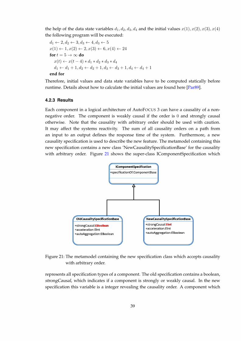
Each component in a logical architecture of AutoFOCUS 3 can have a causality of a non-negative order. The component is weakly causal if the order is 0 and strongly causalotherwise. Note that the causality with arbitrary order should be used with caution.It may affect the systems reactivity. The sum of all causality orders on a path froman input to an output defines the response time of the system. Furthermore, a newcausality specification is used to describe the new feature. The metamodel containing thisnew specification contains a new class ’NewCausalitySpecificationBase’ for the causalitywith arbitrary order. Figure 21 shows the super-class IComponentSpecification which

Figure 21: The metamodel containing the new specification class which accepts causalitywith arbitrary order.

represents all specification types of a component. The old specification contains a boolean,strongCausal, which indicates if a component is strongly or weakly causal. In the newspecification this variable is a integer revealing the causality order. A component which

39

has a new causality specification with the attribute strongCausal = 0, is a weakly causalcomponent. All other components, with strongCausal > 0, are strongly causal.

Conclusion. The result of the causality extension is a new metamodel which containsthe old and new specification. The created system is backward-compatible allowing thedeveloper to use both specifications.

4.3 Implementing the Retiming-Transformation

4.3.1 Motivation

The retiming-transformation is an important technique for changing the causality of asystem. Originally invented for retiming synchronous circuitry [LS91], the retiming-transformation can also be adapted for the logical architecture of AutoFOCUS 3. (seesection 3.3). Retiming changes the causality of the system without affecting the behavioror the end-to-end latency. This is the case for the jitter-robustness optimizing methodpresented in section 3.4.3 which produces a result as a sequence of consecutive appliedretiming-transformations. The aim of this optimization is to maximize the minimumcausality order belonging to some specific components. It is possible that the resultcontains components which are not relevant for the jitter-robustness and thus have acausality order greater than 0. The remaining causalities can be distributed among thesystem in AutoFOCUS 3via retiming-transformation. (e.g. the remaining causalities can beused to increase the parallelism of the system)


For the implementation, the steps presented in section 3.3 for preserving the end-to-endlatency are considered. The algorithm used to implement the retiming-transformation hasto execute the following:

1. Add to the retimed component C the desired amount x of causality. A weakly causalcomponent becomes strongly causal.

2. Find a new predecessor component P which has not been considered yet. If no suchcomponent exists, terminate algorithm.

3. Subtract x from the causality order of P . If P ’s new causality is 0 make it weaklycausal.

4. Find a new successor component S of P which is not component C. If no suchcomponent exists continue with step 2.

5. Delete the channel between P and S.

6. Create a new strongly causal component IDP of order xwhich has one input and oneoutput. This component computes the identity function.

40

7. Add a channel between P and IDP and a channel between IDP and S.

8. Continue with step 4.

In AutoFOCUS 3 each component does not need to have unique names. For eachpredecessor component P there may be more than one IDP components. Therefore, thelogical architecture of the system is easier to understand if the name IDP is extended withthe name of the incoming channel.

4.3.3 Results

In AutoFOCUS 3 any component of the logical architecture can be retimed. Right-clickingthe desired component, a dialog box pops up and shows the interval of numbers inwhich a valid retiming-transformation can be executed. The interval [0..0] states thatthe component can not be retimed. After a component is retimed, the causality ofthe system is updated. The end-to-end latency stays the same. Consequently, theretiming-transformation can influence (positive or negative) some properties like the jitter-robustness or logical tick size of a system. A longer chain of weakly causal componentsas the result of a retiming-transformation increases the logical tick size determined by thecritical path. Also, the retiming-transformation can be used with the help of improvementmethods like the one presented in section 3.4.3. This leads to an optimal jitter-robustnessin the system.

Figure 22: The logical architecture modification of the ACCSystem whose component PCSis retimed with value 2.

41

4.4 Adapting the Code Generator

4.4.1 Motivation

This section provides details about how strongly causal components of a higher orderdelay their outputs in AutoFOCUS 3. In the current implementation of AutoFOCUS 3, thecode generator produces one delay unit for each strongly causal component. This means,the code generator does not support causality with arbitrary order. Therefore, the newmetamodel introduced in figure 21 is adapted to the code generator of AutoFOCUS 3.


For the code generation of a component with arbitrary order, FIFO buffers are used. Eachcomponent possesses for each input port a ring-buffer with the size of its causality. Thesebuffers receive the information that is being sent from the outside and always deliver theoldest message stored. In the first logical ticks the initial values are returned. These are thevalues that are stored in the ring-buffers before runtime.

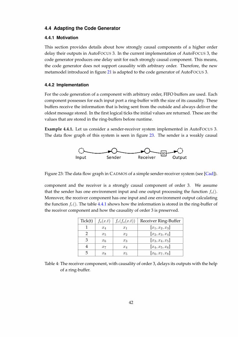
Example 4.4.1. Let us consider a sender-receiver system implemented in AutoFOCUS 3.The data flow graph of this system is seen in figure 23. The sender is a weakly causal

Figure 23: The data flow graph in CADMOS of a simple sender-receiver system (see [Cad]).

component and the receiver is a strongly causal component of order 3. We assumethat the sender has one environment input and one output processing the function fs().Moreover, the receiver component has one input and one environment output calculatingthe function fr(). The table 4.4.1 shows how the information is stored in the ring-buffer ofthe receiver component and how the causality of order 3 is preserved.

Tick(t) fs(x.t) fr(fs(x.t)) Receiver Ring-Buffer1 x4 x1 [x1, x2, x3]2 x5 x2 [x2, x3, x4]3 x6 x3 [x3, x4, x5]4 x7 x4 [x4, x5, x6]5 x8 x5 [x6, x7, x8]

Table 4: The receiver component, with causality of order 3, delays its outputs with the helpof a ring-buffer.

42

4.4.3 Results

A thorough implementation of all necessary features for complete code generation was notwithin the context of this thesis. Nevertheless, the prototypical implementation made wasemployed for the evaluation (see section 5) and has shown to be usable.

4.5 Jitter-Robustness Optimization Implemented in AutoFOCUS 3

4.5.1 Motivation

This section contains information about how the results of the jitter-robustness optimiza-tion method, presented in 3.4.3, are shown in AutoFOCUS 3. It is important for thedeveloper to know which is the highest achievable jitter-robustness. When changing thesystems causality or deployment, the effects on the optimal jitter-robustness can be seen.In this case if the optimum is smaller than the desired robustness, the developer has theoption to revert the changes. Furthermore, it is very hard to determine manually thecausality of each component in a complex system, in order to achieve the optimal jitter-robustness and preserve the end-to-end latency. Industrial relevant systems often havea complex logical architecture and are very hard to analyze. The method presented insection 3.4.3 assures to compute the optimal achievable jitter-robustness by solving a linearproblem. Hence, the developer can adapt the causality of all components on structurallevel according to the variable occupancy of the solved linear system of equations for thejitter-robustness maximization.


Described in section 3.4.3, the optimization of the jitter-robustness has two parts. The firstpart contains the finding of a path coverage that includes all edges of the graph and theconstruction of a system of linear expressions. Finding a path coverage in AutoFOCUS 3, isdone by executing the algorithm explained in pseudocode 1. For each path a new equationis added to the system (see equation 13). In the second part, the solving of the linear systemis effectuated. Lp solve (see [Lp]) is executed with the automatically created script of linearexpressions. After the solver finishes computing, it offers the possibility to visualize thevariable occupancy of the linear system.

4.5.3 Results

The results are seen in AutoFOCUS 3 for each deployment block. Each deploymentcategory has assigned the logical architecture of a root component and a topology(technical architecture) on which the logical system is mapped. By right-clicking thedeployment block and selecting the ’Optimize Jitter-Robustness ...’ action the lp solveprogram starts optimizing the system. A pop-up box, showing each components causalityfor the optimal jitter-robustness appears as soon as the program finds the optimal solution.

43

5 Evaluation

This section contains some practical results of the presented concepts. The aim is to showthat jitter can have negative effects on a system which is not properly retimed. Using theoptimization method from section 3.4.3, the jitter-robustness can improve. The systemcan be immune to jitter that is smaller than ρopt(S) time units. Section 5.1 contains a ’HelloWorld’ example which demonstrates the optimization effects on the system and section 5.2reveals how the jitter-robustness can be improved for the Adaptive Cruise Control modelin AutoFOCUS 3.

5.1 Proof of Concept on Embedded Hardware

5.1.1 Motivation

The jitter-robustness analysis and optimization concepts are evaluated on embeddedhardware. A simple sender-receiver system is supposed to show the importance ofjitter-robustness. This example, reveals a new methodological approach. From a top-down perspective the designer creates a logical model, analyzes its jitter-robustness andimproves it if necessary. All this can be done statically before runtime by using theretiming-transformation appropriately.

5.1.2 Setup

The logical architecture contains two components communicating through a channel. Thefirst component receiving information from the environment is the sender and the secondcomponent sending information to the environment is the receiver. In the first iterationover the system, the sender component has a causality of order 50. This means it sendsthe information received from the environment with a delay of 50 logical ticks. The setupof the logical architecture is visualized with the help of CADMOS (see [Cad]) in figure24. Furthermore, the technical architecture contains two Freescale MPC5554EVB ECU’s

Figure 24: The data flow graph of the analyzed system.

connected with each other through a CAN-Bus. The sender component is deployed onone MPC which receives information from the environment through a potentiometer.The receiver component is deployed on the other MPC which sends information to theenvironment through a servo motor controlled with pulse-width modulation. Both MPC’srun at a frequency of 50 Hz which corresponds to a logical tick of 20 ms. The aimof this setup is to control remotely the servo motor from the receiving MPC with the

44

potentiometer from the sending MPC. In order to make jitter even more dangerous, deltavalues are sent on the bus. This means, the sender returns the difference between the lastvalue and the current value received from the potentiometer. If a message is lost, the servomotor points at a different value than the one read by the sender board.

Creating jitter. Two MPC5554EVB ECU’s connected to the same CAN-Bus are used tocreate jitter. If both send at a 1 kHz frequency dummy messages with a higher priorityon the bus, the sender reduces his sending rate. Therefore, the information comes to slowto the receiver and jitter is produced. Figure 25 represents the technical architecture of

3

1

2

4

5

7

6

Figure 25: The embedded hardware which represents the technical architecture of thesystem.

the system. MPC’s 1 and 2 are the sender/receiver components communicating throughCAN-Bus 5. 6 shows the potentiometer reading environment inputs and 7 is the servomotor actuator. MPC’s 3 and 4 are used to create bus load in order to produce conflictsthat delay the sending routine. If these two MPC’s 3 and 4 run simultaneously, thesystem looses information and the servo motors position will no longer correspond tothe potentiometers value. In this example the worst case execution time (WCET) for acomponent is≈ 6µswhich is much lower than the logical tick, 20ms. Therefore, if the jitteris lower than ≈ 20ms − 6µs the receiver component can still produce an output in time.That is why one MPC is insufficient for the disturbance of the system behavior.

45

5.1.3 Analysis and Transformation

The first step is to analyze this system S shown in figure 24. Regarding section 3.2, thesystem has ρ(S) = 0. In this case the developer should analyze the bus load carefully. Forsystems which send delta values, jitter-robustness is essential. It can occur that a messagethat comes too late has as consequence for the system to run out of sync and produceincorrect outputs. This example deals with a system which has one input and one outputwith a end-to-end latency of 50 time units. The jitter-robustness is 0 because the causality ofthe receiver component is 0. However, this model can be improved. For the optimal jitter-robustness the receiver component has to be retimed with the maximal possible value50. The resulting data flow graph of the transformed system is seen in figure 26. The

Figure 26: The data flow graph of the transformed, jitter-robust system.

optimal jitter-robustness does not exceed 50 logical ticks which is equal to the latency fromthe input to the output. In the section 5.1.2, it is stated that the MPC’s, on which thecomponents are deployed, run at a 50 Hz frequency. This means, they produce an outputevery 20 ms. Therefore, having a jitter-robustness of 50 ticks means that the informationcan come 1 second later and the produced output is correct.

5.1.4 Results

For this example, the optimal jitter-robust system is created. Jitter smaller than one seconddoes not affect the output. The result is seen when the two MPC’s which create bus loadare turned on for less than one second. The system does not change its behavior. Anotherway to test the jitter-robustness is to unplug the CAN-Bus cable. Removing the cable forless than one second from a MPC causes the receiver buffer to run almost empty but notloose any data. This scenario is described with the help of table 5.1.4. Notice how after theCAN-Bus cable is plugged in, the receiver ring-buffer gets all the elements that have notbeen transmitted. This is done by the CAN-Driver which stores the messages in an internalbuffer, if the sending is unsuccessful. After the cable is plugged in, all the messages storedin the CAN-Driver buffer are sent to the receiver. In this way the receiver buffer becomesfull again and the system is ready for new jitter to occur.

5.1.5 Discussion

For this system, the optimal jitter-robustness must not necessarily be achieved. Theoriginal system whose jitter-robustness is 0 needs two MPC’s, which submit dummy

46

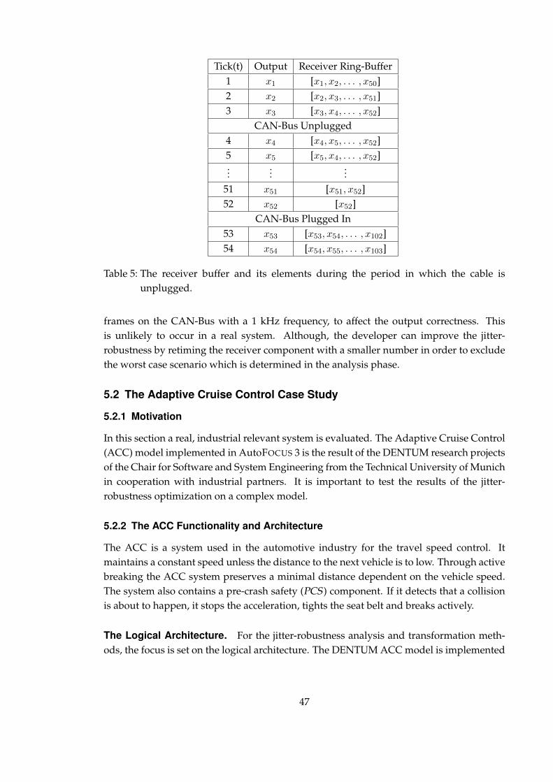
Tick(t) Output Receiver Ring-Buffer1 x1 [x1, x2, . . . , x50]2 x2 [x2, x3, . . . , x51]3 x3 [x3, x4, . . . , x52]

CAN-Bus Unplugged4 x4 [x4, x5, . . . , x52]5 x5 [x5, x4, . . . , x52]...

......

51 x51 [x51, x52]52 x52 [x52]

CAN-Bus Plugged In53 x53 [x53, x54, . . . , x102]54 x54 [x54, x55, . . . , x103]

Table 5: The receiver buffer and its elements during the period in which the cable isunplugged.

frames on the CAN-Bus with a 1 kHz frequency, to affect the output correctness. Thisis unlikely to occur in a real system. Although, the developer can improve the jitter-robustness by retiming the receiver component with a smaller number in order to excludethe worst case scenario which is determined in the analysis phase.

5.2 The Adaptive Cruise Control Case Study

5.2.1 Motivation

In this section a real, industrial relevant system is evaluated. The Adaptive Cruise Control(ACC) model implemented in AutoFOCUS 3 is the result of the DENTUM research projectsof the Chair for Software and System Engineering from the Technical University of Munichin cooperation with industrial partners. It is important to test the results of the jitter-robustness optimization on a complex model.

5.2.2 The ACC Functionality and Architecture

The ACC is a system used in the automotive industry for the travel speed control. Itmaintains a constant speed unless the distance to the next vehicle is to low. Through activebreaking the ACC system preserves a minimal distance dependent on the vehicle speed.The system also contains a pre-crash safety (PCS ) component. If it detects that a collisionis about to happen, it stops the acceleration, tights the seat belt and breaks actively.

The Logical Architecture. For the jitter-robustness analysis and transformation meth-ods, the focus is set on the logical architecture. The DENTUM ACC model is implemented

47

in AutoFOCUS 3 and contains seven strongly causal atomic components of order one:PCS, DesiredSpeed, SpeedControl, CoreArbiter, DesiredDistance, DistanceControl andOnOffArbiter. We analyze a modified version of the DENTUM ACC model wherethe new components ConstInputACC, ConstantSensorEmulation, ConstInputPCS andSensorProcessing are used to generate inputs. The data flow graph of the model is seenin figure 27. In order to make things clearer, the environment ports have been left out.The logical architecture of the root component and the hierarchical structure are shown in

Figure 27: The data flow graph of the modified DENTUM ACC model visualized withCADMOS.

figure 28. ACCSystem is the root component of the DENTUM ACC system. It includestwo components, ACC and PCS, which communicate with each other through the channelpcsSuspend. The ACC system receives from environment inputs regarding the state ofthe system (accOnOff ), the gas and brake pedal positions (gasPedal, brakePedal ) and therequest to change distance or to increase/decrease the vehicle speed (changeDistance,incDecDesiredSpeed ). It calculates the acceleration and sends it through the outputport outputAcc to the environment. Multicast input ports send information, about theexistence and distance to the vehicle ahead and the speed, to both components, ACC andPCS. Furthermore, PCC receives information about the belt and brake status (beltReady,

48

brakeReady). It also has the ability to stop the acceleration of the ACC component bysending the value ’true’ on the pcsSuspend channel. This can be the case if the distance inmeter to the next vehicle is smaller than the half of the vehicle speed. The pre-crash safetysystem also has the duty to brake and show a warning if a collision is detected.

(a) (b)

Figure 28: The hierarchical view of the ACCSystem in figure (a) and the logical architectureof the root component in figure (b).

5.2.3 Possible Results of the Jitter-Robustness Optimization

There are many possibilities to deploy the logical architecture on two ECU’s of typeMPC5554 connected through a CAN-Bus. This section contains the analysis regardingthe jitter-robustness optimization of two different deployment mappings.

Deployment 1. All the components which belong to the ACC system are mapped tothe first MPC and the PCS component to the second MPC. Hence, the CAN-Bus hasto transmit the safety critical information of the channel pcsSuspend and the messagescoming from the SensorProcessing component on channels vSpeed, targetExists andtargetDistance. This mapping is intuitive and has relative little bus load (see figure 29).The value transmitted on the channel pcsSuspend is mostly ’false’. The safety criticalvalue ’true’ is sent only if a collision is detected. For analyzing the jitter-robustness ofthe system with this deployment, the following observations are taken into account. Allcomponents are strongly causal of order one. This means, the jitter-robustness is greateror equal to one time unit. Because the OnOffArbiter component receives information fromthe bus and sends information to the environment port output with one delay unit, the

49

jitter-robustness is exactly one logical tick. Using the optimization method presented insection 3.4 and implemented in AutoFOCUS 3 (see section 4.5), the optimal jitter-robustnessis also one time unit. In this case the optimal jitter-robustness is already achieved. Nochanges need to be done to the model. This deployment mapping can not produce for thesystem a jitter-robustness greater than one.

Figure 29: The first deployment mapping realized in AutoFOCUS 3 of the DENTUM ACCsystem.

Deployment 2. The second deployment mapping gets the OnOffArbiter and the Core-Arbiter on the first MPC and the rest of the ACC system and the PCS component onthe second MPC. This mapping is seen in figure 30. The CAN-Bus transmits the inputsgenerated in the SensorProcessing and ConstInputACC components. Moreover, the busalso sends the messages on the channels constantSpeedAccel, followUpAccel, speedCapand suspend. All this messages are safety critical and need to be jitter-robust. For thejitter-robustness analysis we make the same two observations as with deployment 1 andthe result is one time unit. A advantage of this deployment mapping is the possibilityto improve the jitter-robustness. With the help of the optimization method implementedin AutoFOCUS 3 (see section 4.5) the developer finds out how to make the system robustagainst two logical ticks of jitter. The result of the jitter-robustness optimization assignsboth components OnOffArbiter and CoreArbiter a causality of order two. Therefore, theoptimal robustness against jitter is twice as big as the one in the original system.

5.2.4 Discussion

Without the proper algorithm for retiming the DENTUM ACC system, it is very hard toimprove the jitter-robustness manually. With the help of the methods from section 3, we

50

Figure 30: The second deployment mapping realized in AutoFOCUS 3 of the DENTUMACC system.

analyzed two different deployment mappings and realized that both lead to a differentoptimal jitter-robustness. The first mapping does not bring any improvements to it,whereas the second one doubles its value. Hence, the deployment mapping influencesdirectly the value of the jitter-robustness and its optimum. The method used in the secondmapping was to deploy the components which deliver safety critical outputs on an ownMPC. This heuristic causes the robustness optimization algorithm to improve where it ismost needed.

51

6 Discussion

In this section we take a closer look to the presented aspects of this thesis. The previoussections bring a definition to the jitter-robustness (section 3.1), an analysis technique tocalculate it (section 3.2) and an optimization method for improving its value (section 3.4.3).An example of a system on embedded hardware shows the validity of these analysis andimprovement procedures (section 5.1). Moreover, the case tool AutoFOCUS 3 has beenthe main tool for testing the jitter-robustness with real models. Some of the analysisand transformation methods have been implemented in AutoFOCUS 3 and used on theDENTUM Adaptive Cruise Control model (section 5.2). By choosing the right deploymentthe jitter-robustness of the DENTUM ACC model can be improved to be twice as big (seesection 5.2.3). However, some questions still need to be clarified.

What are the trade-offs of optimizing the jitter-robustness? When designing asystem the developer has to know regarding the inter-processor communication howmuch bus load there is in a worst case scenario. A strong analysis during the designingphase leads to a conclusion, whether the jitter-robustness of the system is sufficient ornot. It is not necessary to change the system to obtain the optimal jitter-robustness if itis not needed. Nevertheless, the optimization method suggests if the constructed systemcan be robust against jitter. If the optimal jitter-robustness is not sufficient to cover theworst case scenario of jitter, the developer should consider adding more causality to thesystem or changing the deployment mapping. Furthermore, achieving the optimal jitter-robustness can damage other properties of the system like performance or parallelism. Itis the developers task to find a way to preserve a certain amount of all properties.

Is there a connection between the jitter-robustness and the reactivity of a system?The two terms jitter-robustness and reactivity are two properties of a system which areopposite. This means, a system with a higher jitter-robustness value has a lower reactivitylevel. The other way must not necessarily hold. A lower reactivity level can have both ahigh and a low jitter-robustness. Regarding section 3.2, the jitter-robustness is calculatedby searching the minimal delayed path from a component which receives bus informationto an output. If the robustness against jitter is high, the end-to-end latency on that path isalso high and this results to a low reactivity. The other way, if the reactivity is low, all thecausality delays must not necessarily be on that minimal path to an output.

What happens after the optimization with the causalities that are irrelevant for thejitter-robustness? After the optimization some components can receive causality of ahigher order even if they do not improve the jitter-robustness. In this case the developerchooses the distribution of the remaining causality after other criteria. For example, thedeveloper can decide to improve the parallelism or improve the performance by adjustingthe minimal clock period time.

52

Is the jitter-robustness optimization method customizable? It is described in section3.4.3 how to achieve the optimal jitter-robustness by changing the logical architecture in asystem. However, components which deliver safety critical outputs must be robust againstjitter. Hence, the optimizing method can be adjusted to improve the jitter-robustness forspecific components. This is done by selecting those components in the inequality partof the linear problem (see section 3.4.3) which deliver safety critical outputs. The entiresystem can have a lower jitter-robustness value than the optimum but the reliability on thesafety critical outputs is higher.

What are the results of this thesis? The results of this thesis are the jitter-robustnessanalysis and optimization methods, the retiming-transformation adapted to the logicalarchitecture and the evaluation of the industrial DENTUM ACC model. Jitter-robustnessis expressed in logical ticks using the analysis method presented in section 3.2. The formalmethod for achieving the optimal jitter-robustness is described in section 3.4.3 by creatinga linear problem. An advantage of this procedure is its scalability. The optimal resultis produced for the industrial relevant Adaptive Cruise Control model implemented inAutoFOCUS 3 in less than 0.1 seconds on a Intel(R) Core(TM)2 Duo CPU with 2.4GHz.

53

7 Conclusion and Future Work

Jitter-robustness is an important property of embedded multiprocessor systems. Itimproves the quality insurance. After the analysis method presented in section 3.2, thedeveloper decides if the robustness against jitter needs to be improved. The optimizationmethod in section 3.4.3 indicates the maximal jitter-robustness which can be achievedregarding the logical and technical perspective together with their deployment mapping.

Improving the jitter-robustness on behavior level as future work. The focus is setinside the logical tick. Making the duration of a tick longer adds jitter-robustness to thesystem. However, this affects the performance of the system. Jitter-robustness can alsobe improved on behavior level by choosing an adequate scheduling algorithm. Finding aheuristic for the task execution order can lead to a higher jitter-robustness (see figure 31).

Number of ECU’s

Logical Ticks

P1

P2

1 2

Jitter-Robustness

Jitter-Robustness

Task1

Task2

Task1

A

Task2

Figure 31: Improving jitter-robustness with scheduling.

Heuristic for finding the optimal deployment concerning the jitter-robustness. Asseen in section 5.2.3, a different deployment mapping can lead to a higher jitter-robustnessof the system. A brute-force approach for iterating through all possible deploymentmappings can be very time consuming. Finding a good heuristic for choosing a jitter-robust deployment remains an open area for research.

Testing the optimization algorithm on complex models. Industry-relevant systemscan contain many components and channels. Achieving the optimal jitter-robustness insuch a system manually is very hard. The automated algorithm (see section 3.4.3) is usedto observe how much more jitter-robustness can be achieved. Testing this method on largermodels can make statements about its scalability.

54

List of Figures

1 A logical architecture deployed on a technical architecture. . . . . . . . . . . 82 The model, metamodel and meta-metamodel of a state diagram. . . . . . . . 103 Different granularity levels (vertical) and different software development

perspectives (horizontal) according to [TRS+10]. . . . . . . . . . . . . . . . . 114 The external interface of the filtering function with two inputs and one

output channel. . . . . . . . . . . . . . . . . . . . . . . . . . . . . . . . . . . . 135 The data flow program and data flow graph. . . . . . . . . . . . . . . . . . . 156 The two possible retiming-transformations that can be executed on a com-

ponent. . . . . . . . . . . . . . . . . . . . . . . . . . . . . . . . . . . . . . . . . 177 AutoFOCUS 3 structural and automaton view . . . . . . . . . . . . . . . . . . 198 The translation of the weakly and strongly causal components to homoge-

neous iterative data flow graphs.[Sch11] . . . . . . . . . . . . . . . . . . . . . 219 The definition of jitter and the jitter-deviation which is analyzed and

handled in this thesis. . . . . . . . . . . . . . . . . . . . . . . . . . . . . . . . . 2310 A valid AutoFOCUS 3 model satisfying the necessary constraints for jitter-

robustness analysis in this thesis. . . . . . . . . . . . . . . . . . . . . . . . . . 2511 The first step of the retiming-transformation in a logical architecture. . . . . 2712 The second step of the retiming-transformation in a logical architecture. . . 2713 The third step of the retiming-transformation in a logical architecture. . . . 2814 The forth step of the retiming transformation in a logical architecture. . . . . 2815 First basic scenario for improving the jitter-robustness. . . . . . . . . . . . . 2916 Second basic scenario for improving the jitter-robustness. . . . . . . . . . . . 3017 Third basic scenario for improving the jitter-robustness. . . . . . . . . . . . . 3118 The data flow graph containing the eight strongly causal components of the

system. . . . . . . . . . . . . . . . . . . . . . . . . . . . . . . . . . . . . . . . . 3419 Each output of a component with its guaranteed delays. The value ’X’ is

shown for those outputs which do not communicate with any environmentinput ports. . . . . . . . . . . . . . . . . . . . . . . . . . . . . . . . . . . . . . . 36

20 The data flow graph of a strongly causal component of order 4. . . . . . . . 3821 The metamodel containing the new specification class which accepts causal-

ity with arbitrary order. . . . . . . . . . . . . . . . . . . . . . . . . . . . . . . 3922 The logical architecture modification of the ACCSystem whose component

PCS is retimed with value 2. . . . . . . . . . . . . . . . . . . . . . . . . . . . . 4123 The data flow graph in CADMOS of a simple sender-receiver system. . . . . 4224 The data flow graph of the sender-receiver system. . . . . . . . . . . . . . . . 4425 The embedded hardware which represents the technical architecture of the

system. . . . . . . . . . . . . . . . . . . . . . . . . . . . . . . . . . . . . . . . . 4526 The data flow graph of the transformed, jitter-robust sender-receiver system. 4627 The data flow graph of the modified DENTUM ACC model visualized with

CADMOS. . . . . . . . . . . . . . . . . . . . . . . . . . . . . . . . . . . . . . . . 48

55

28 The hierarchical view of the ACCSystem in figure (a) and the logicalarchitecture of the root component in figure (b). . . . . . . . . . . . . . . . . 49

29 The first deployment mapping realized in AutoFOCUS 3 of the DENTUMACC system. . . . . . . . . . . . . . . . . . . . . . . . . . . . . . . . . . . . . . 50

30 The second deployment mapping realized in AutoFOCUS 3 of the DENTUMACC system. . . . . . . . . . . . . . . . . . . . . . . . . . . . . . . . . . . . . . 51

31 Improving jitter-robustness with scheduling. . . . . . . . . . . . . . . . . . . 54

56

List of Tables

1 FOCUS specification of a system. . . . . . . . . . . . . . . . . . . . . . . . . . 132 FOCUS specification of component F . . . . . . . . . . . . . . . . . . . . . . . 143 The sequence of retiming-transformations leading to the optimal jitter-

robustness. . . . . . . . . . . . . . . . . . . . . . . . . . . . . . . . . . . . . . . 354 The receiver component, with causality of order 3, delays its outputs with

the help of a ring-buffer. . . . . . . . . . . . . . . . . . . . . . . . . . . . . . . 425 The receiver buffer and its elements during the period in which the cable is

unplugged. . . . . . . . . . . . . . . . . . . . . . . . . . . . . . . . . . . . . . . 47

57

References

[Ack82] W.B. Ackerman. Data flow languages. Computer;(United States), 2, 1982.

[Aut] AutoFocus 3 Homepage. http://af3.in.tum.de/.

[BA81] J. Brock and W. Ackerman. Scenarios: A model of non-determinatecomputation. In Formalization of programming concepts, pages 252–259. Springer,1981.

[BFG+08] Manfred Broy, Martin Feilkas, Johannes Grunbauer, Alexander Gruler, Alexan-der Harhurin, Judith Hartmann, Birgit Penzenstadler, Bernhard Schatz, andDoris Wild. Umfassendes Architekturmodell fur das Engineering eingebetteterSoftware-intensiver Systeme. Technical Report TUM-I0816, Technische Univer-sitat Munchen, jun 2008.

[Bro10] M. Broy. Relating time and causality in interactive distributed systems. EuropeanReview, 18(04):507–563, 2010.

[BS01] M. Broy and K. Stoelen. Specification and development of interactive systems:Focus on streams, interfaces, and refinement, 2001.

[Cad] Cadmos is a tool used to visualize, analyze and transform data-flow graphsdeveloped at the Technical University of Munich, Chair IV for Software andSystem Engineering. http://code.google.com/a/eclipselabs.org/p/cadmos/.

[Den80] J.B. Dennis. Data flow supercomputers. Computer, 13(11):48–56, 1980.

[DK82] A.L. Davis and R.M. Keller. Data flow program graphs. Computer, 15(2):26–41,1982.

[Gmb] Robert BOSCH GmbH. CAN Specification, Version 2.0., 1991.

[HHR09] Alexander Harhurin, Judith Hartmann, and Daniel Ratiu. Motivation andFormal Foundations of a Comprehensive Modeling Theory for EmbeddedSystems. Technical Report TUM-I0924, Technische Universitat Munchen, 2009.

[HS01] F. Huber and B. Schatz. Integrated development of embedded systems withautofocus. Technische Universitat Munchen, Fakultat fur Informatik, 7, 2001.

[HST10] F. Hoelzl, M. Spichkova, and D. Trachtenherz. AutoFocus Tool Chain.techreport, Technische Universitaet Muenchen, 2010.

[Lp] Homepage of the software lp solve used to compute results for linear problems.http://lpsolve.sourceforge.net/.

[LS91] C.E. Leiserson and J.B. Saxe. Retiming synchronous circuitry. Algorithmica,6(1):5–35, 1991.

58

[MOF] Object Management Group MOF. OMG’s MetaObject Facility (MOF) Home-page. http://www.omg.org/mof.

[Par89] K.K. Parhi. Algorithm transformation techniques for concurrent processors.Proceedings of the IEEE, 77(12):1879–1895, 1989.

[PFTV] WH Press, BP Flannery, SA Teukolsky, and WT Vetterling. Cyclic redundancyand other checksums. Ch. 20.3 in Numerical Recipes in FORTRAN: The Art ofScientific Computing, pages 888–895.

[Res] Microsoft Research. SMT-Solver Z3 is an efficient theoremprover being developed at Microsoft Research.The homepage is:http://research.microsoft.com/en-us/um/redmond/projects/z3/.

[RST09] Daniel Ratiu, Wolfgang Schwitzer, and Judith Thyssen. A System ofAbstraction Layers for the Seamless Development of Embedded SoftwareSystems. Technical report, Technische Universitat Munchen, nov 2009.

[Sch11] Wolfgang Schwitzer. Concurrency Analysis and Transformation - An Overview.Technical report, Technische Universitat Munchen, 2011.

[TRS+10] J. Thyssen, D. Ratiu, W. Schwitzer, A. Harhurin, M. Feilkas, and E. Thaden.A System for Seamless Abstraction Layers for Model-based Development ofEmbedded Software. In Software Engineering (Workshops), 2010.

59

Concept and Implementation of a Jitter-Robustness...

Documents

Transcript of Concept and Implementation of a Jitter-Robustness...