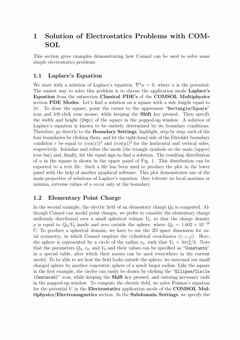
1 Solution of Electrostatics Problems with COM-

SOL

This section gives examples demonstrating how Comsol can be used to solve somesimple electrostatics problems.

1.1 Laplace’s Equation

We start with a solution of Laplace’s equation, ∇2u = 0, where u is the potential.The easiest way to solve this problem is to choose the application mode Laplace’sEquation from the subsection Classical PDE’s of the COMSOL Multiphysicssection PDE Modes. Let’s find a solution on a square with a side length equal to2π. To draw the square, point the cursor to the uppermost “Rectangle/Square”icon and left-click your mouse, while keeping the Shift key pressed. Then specifythe width and height (2*pi) of the square in the popped-up window. A solution ofLaplace’s equation is known to be entirely determined by its boundary conditions.Therefore, go directly to the Boundary Settings, highlight, step by step, each of thefour boundaries by clicking them, and let the right-hand side of the Dirichlet boundarycondition r be equal to (cos(x))2 and (cos(y))2 for the horizontal and vertical sides,respectively. Initialize and refine the mesh (the triangle symbols on the main (upper)icon bar) and, finally, hit the equal sign to find a solution. The resulting distributionof u in the square is shown in the upper panel of Fig. 1. This distribution can beexported to a text file. Such a file has been used to produce the plot in the lowerpanel with the help of another graphical software. This plot demonstrates one of themain properties of solutions of Laplace’s equation: they tolerate no local maxima orminima, extreme values of u occur only at the boundary.

1.2 Elementary Point Charge

In the second example, the electric field of an elementary charge Q0 is computed. Al-though Comsol can model point charges, we prefer to consider the elementary chargeuniformly distributed over a small spherical volume V0, so that the charge densityρ is equal to Q0/V0 inside and zero outside the sphere, where Q0 = 1.602 × 10−19

C. To produce a spherical domain, we have to use the 2D space dimension for ax-ial symmetry, in which Comsol employs the cylindrical coordinates (r, z, ϕ). Here,the sphere is represented by a circle of the radius r0, such that V0 = 4πr30/3. Notethat the parameters Q0, r0, and V0 and their values can be specified as “Constants”in a special table, after which their names can be used everywhere in the currentmodel. To be able to see how the field looks outside the sphere, we surround our smallcharged sphere by another concentric sphere of a much larger radius. Like the squarein the first example, the circles can easily be drawn by clicking the “Ellipse/Circle(Centered)” icon, while keeping the Shift key pressed, and entering necessary radiiin the popped-up window. To compute the electric field, we solve Poisson’s equationfor the potential V in the Electrostatics application mode of the COMSOL Mul-tiphysics/Electromagnetics section. In the Subdomain Settings, we specify the

values of ρ in our two subdomains (the charged small sphere and empty large sphere)and the value of εr = 1 for the relative permittivity in either of them. In the Bound-ary Settings, we choose the “Ground” and “Continuity” conditions for the outer andinner spheres, respectively. The final two steps are to mesh the subdomains and solvethe problem. The upper panel of Fig. 2 presents the solution in a form that can becustomized using a number of options in the Postprocessing section. It is convenientthat the Comsol solution contains not only the dependent variable (the potential V inthe present case) but also its various derivatives. One of such derivatives gives the ra-dial (in the cylindrical coordinates) component of the electric field Er. Its ratio to therespective expression from Coulomb’s law is plotted in the lower panel for z = 0. Thelower plot is obtained using the option Line/Extrusion of the Cross-Section plotParameters section in Postprocessing. You can play with different postprocessingoptions to figure out what they do or you can read the COMSOL Multiphysics User’sGuide that is downloaded as a web page with other Comsol reference pages when youclick the button Help, wherever you see it.

1.3 Electric Dipole

The third example is an electric dipole consisting of two opposite elementary chargesuniformly distributed over two small spheres that are separated by a specified distance.This problem is similar to the previous one, therefore it can be used as an exercise.Its solution is shown in Fig. 3.

1.4 Faraday’s Cage

The fourth example is a model of Faraday’s cage, i.e. an enclosure made of a conductingmaterial (e.g., steel) placed in a strong external electric field. It shows that the Faradaycage blocks out the external static electric field, like a shield. We use the 2D spacedimension that employs Cartesian coordinates (x, y, z). In the XY-plane of the screenthe enclosure is represented by a square with sides of a finite thickness (to obtain it,draw two squares with slightly different side lengths, highlight both of them by pressingCtrl-A, and click the icon “Difference” that will subtract the smaller square fromthe larger one. Outline the enclosure by a square of a larger radius. In the BoundarySettings, prescribe the upper side of the large square a high potential, e.g. V = 1000V, and let its lower side be at “Ground” (V = 0). The left and right sides of the largesquare should be in “Electric insulation”. All sides of the enclosure are subjectto the “Continuity” interior boundary conditions. In the Subdomain Settings, weleave all the standard settings, except the electric conductivity of the enclosure wallsfor which we use the value of σ = 4.032× 106 [S/m] for steel. The final two steps areto mesh the subdomains and solve the problem, as usually. The resulting distributionof the electric field and potential are shown in Fig. 4. We see that the strong externalfield does not penetrate the enclosure, therefore it is actually safe to be in a car (nota convertible though!) during a thunderstorm.

2

1.5 Electric Sensor

The final electrostatics example is based on one of the pre-tested models supplied withthe COMSOL package. This is a model of “electric sensor”, the original versionof which can be found in the COMSOL Multiphysics/Electromagnetics sectionof the Model Library. The electric sensor is a box inside of which there are objectsof different forms with different relative permittivities (in this example, the hiddenobjects are the letters “UVic” with the permittivities 2, 3, 4, and 5, respectively).The objects do not touch the lower and upper boundaries of the box. The lowerboundary is grounded (V = 0), while the upper boundary has the potential V = 1 V.The resulting potential difference produces an electric field directed from the upper tolower boundary that induces a surface charge on the boundaries. The surface chargedensity depends on the permittivity and form of the objects that are encountered bythe electric field on its way in the box (Fig. 5). This allows us to see the box’s contentthrough its boundaries.

2 Solution of Magnetostatics Problems with COM-

SOL

This section presents three examples of magnetostatics problems that are solved usingpre-tested models from Comsol’s Model Library. They are followed by a descriptionof our original Comsol model designed to simulate a small puck magnet falling througha long copper tube.

2.1 Eddy Currents

The first example is a tutorial model of eddy currents (the blue region in Fig. 6)induced in a metallic cylinder by an alternating current in a surrounding coil. Only across-section of the coil wire is shown in the figure (the red circle). It is seen that thecurrent in the cylinder has a direction opposite to that of the current in the coil (theblue and red colors, respectively). This is a consequence of the well-known general rulesaying that (eddy) currents generated in a conductor by a varying magnetic flux (inthe present example, it is produced by the alternating current) have such orientationand strength that their associated magnetic field counteracts the flux change that hascaused their generation. The distribution of the current density in the coil (the currentis stronger near the surface of the wire) demonstrates the so-called “skin effect” in aconductor with an alternating current – a shift of the current toward the conductor’ssurface, which is also caused by eddy currents but now in the coil. This problem issolved in the 2D axisymmetric geometry. Streamlines of the magnetic field are alsoshown.

3

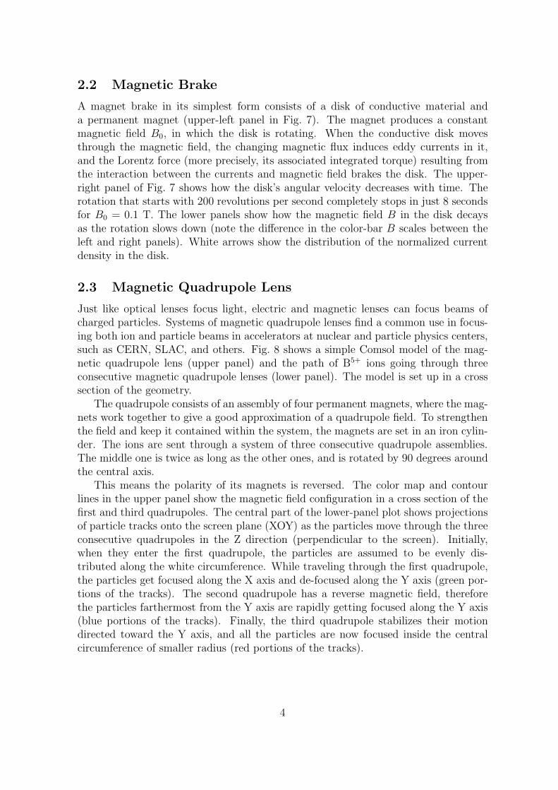
2.2 Magnetic Brake

A magnet brake in its simplest form consists of a disk of conductive material anda permanent magnet (upper-left panel in Fig. 7). The magnet produces a constantmagnetic field B0, in which the disk is rotating. When the conductive disk movesthrough the magnetic field, the changing magnetic flux induces eddy currents in it,and the Lorentz force (more precisely, its associated integrated torque) resulting fromthe interaction between the currents and magnetic field brakes the disk. The upper-right panel of Fig. 7 shows how the disk’s angular velocity decreases with time. Therotation that starts with 200 revolutions per second completely stops in just 8 secondsfor B0 = 0.1 T. The lower panels show how the magnetic field B in the disk decaysas the rotation slows down (note the difference in the color-bar B scales between theleft and right panels). White arrows show the distribution of the normalized currentdensity in the disk.

2.3 Magnetic Quadrupole Lens

Just like optical lenses focus light, electric and magnetic lenses can focus beams ofcharged particles. Systems of magnetic quadrupole lenses find a common use in focus-ing both ion and particle beams in accelerators at nuclear and particle physics centers,such as CERN, SLAC, and others. Fig. 8 shows a simple Comsol model of the mag-netic quadrupole lens (upper panel) and the path of B5+ ions going through threeconsecutive magnetic quadrupole lenses (lower panel). The model is set up in a crosssection of the geometry.

The quadrupole consists of an assembly of four permanent magnets, where the mag-nets work together to give a good approximation of a quadrupole field. To strengthenthe field and keep it contained within the system, the magnets are set in an iron cylin-der. The ions are sent through a system of three consecutive quadrupole assemblies.The middle one is twice as long as the other ones, and is rotated by 90 degrees aroundthe central axis.

This means the polarity of its magnets is reversed. The color map and contourlines in the upper panel show the magnetic field configuration in a cross section of thefirst and third quadrupoles. The central part of the lower-panel plot shows projectionsof particle tracks onto the screen plane (XOY) as the particles move through the threeconsecutive quadrupoles in the Z direction (perpendicular to the screen). Initially,when they enter the first quadrupole, the particles are assumed to be evenly dis-tributed along the white circumference. While traveling through the first quadrupole,the particles get focused along the X axis and de-focused along the Y axis (green por-tions of the tracks). The second quadrupole has a reverse magnetic field, thereforethe particles farthermost from the Y axis are rapidly getting focused along the Y axis(blue portions of the tracks). Finally, the third quadrupole stabilizes their motiondirected toward the Y axis, and all the particles are now focused inside the centralcircumference of smaller radius (red portions of the tracks).

4

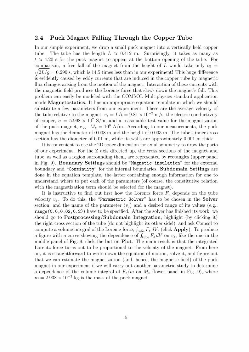
2.4 Puck Magnet Falling Through the Copper Tube

In our simple experiment, we drop a small puck magnet into a vertically held coppertube. The tube has the length L ≈ 0.412 m. Surprisingly, it takes as many ast ≈ 4.20 s for the puck magnet to appear at the bottom opening of the tube. Forcomparison, a free fall of the magnet from the height of L would take only tff =√

2L/g = 0.290 s, which is 14.5 times less than in our experiment! This huge differenceis evidently caused by eddy currents that are induced in the copper tube by magneticflux changes arising from the motion of the magnet. Interaction of these currents withthe magnetic field produces the Lorentz force that slows down the magnet’s fall. Thisproblem can easily be modeled with the COMSOL Multiphysics standard applicationmode Magnetostatics. It has an appropriate equation template in which we shouldsubstitute a few parameters from our experiment. These are the average velocity ofthe tube relative to the magnet, v

z= L/t = 9.81× 10−2 m/s, the electric conductivity

of copper, σ = 5.998 × 107 S/m, and a reasonable test value for the magnetizationof the puck magnet, e.g. M

z= 106 A/m. According to our measurements, the puck

magnet has the diameter of 0.008 m and the height of 0.003 m. The tube’s inner crosssection has the diameter of 0.01 m, while its walls are approximately 0.001 m thick.

It is convenient to use the 2D space dimension for axial symmetry to draw the partsof our experiment. For the Z axis directed up, the cross sections of the magnet andtube, as well as a region surrounding them, are represented by rectangles (upper panelin Fig. 9). Boundary Settings should be “Magnetic insulation” for the externalboundary and “Continuity” for the internal boundaries. Subdomain Settings aredone in the equation template, the latter containing enough information for one tounderstand where to put each of the parameters (of course, the constitutive relationwith the magnetization term should be selected for the magnet).

It is instructive to find out first how the Lorentz force Fzdepends on the tube

velocity vz. To do this, the “Parametric Solver” has to be chosen in the Solver

section, and the name of the parameter (vz) and a desired range of its values (e.g.,

range(0.0,0.02,0.2)) have to be specified. After the solver has finished its work, weshould go to Postprocessing/Subdomain Integration, highlight (by clicking it)the right cross section of the tube (do not highlight its other side!), and ask Comsol tocompute a volume integral of the Lorentz force,

∫

tube FzdV , (click Apply). To produce

a figure with a curve showing the dependence of∫

tube FzdV on v

z, like the one in the

middle panel of Fig. 9, click the button Plot. The main result is that the integratedLorentz force turns out to be proportional to the velocity of the magnet. From hereon, it is straightforward to write down the equation of motion, solve it, and figure outthat we can estimate the magnetization (and, hence, the magnetic field) of the puckmagnet in our experiment if we will carry out another parametric study to determinea dependence of the volume integral of F

z/m on M

z(lower panel in Fig. 9), where

m = 2.938× 10−3 kg is the mass of the puck magnet.

5

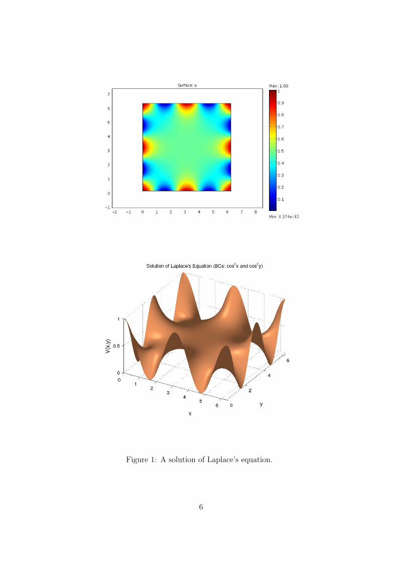
Figure 1: A solution of Laplace’s equation.

6

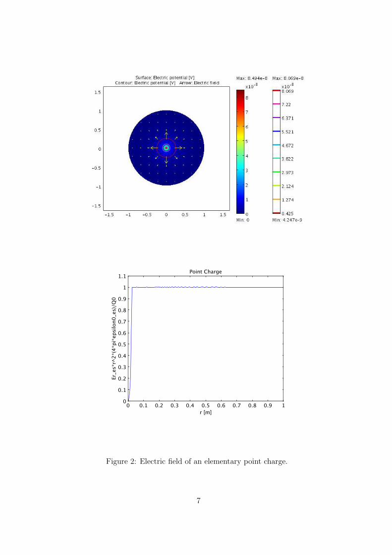
Figure 2: Electric field of an elementary point charge.

7

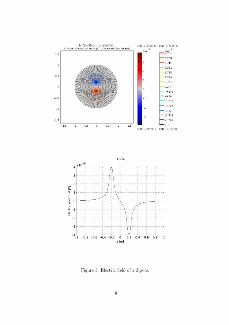
Figure 3: Electric field of a dipole.

8

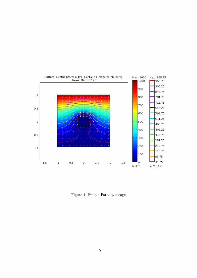
Figure 4: Simple Faraday’s cage.

9

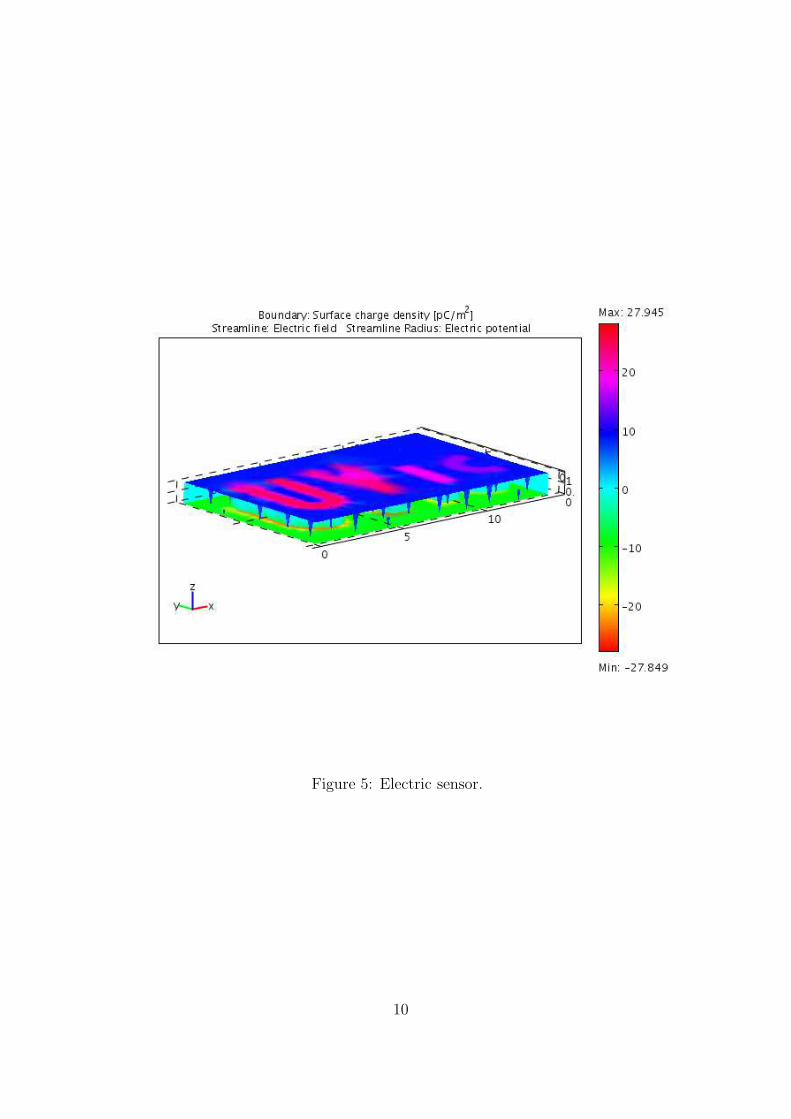
Figure 5: Electric sensor.

10

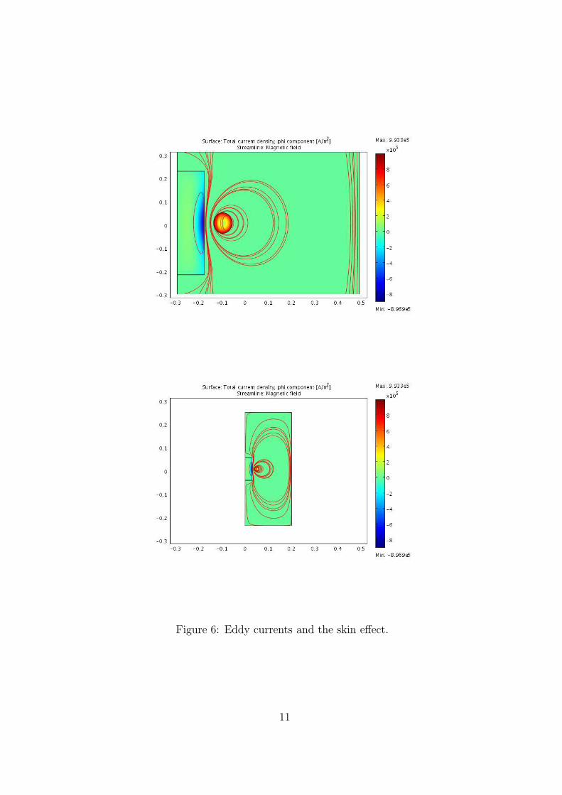
Figure 6: Eddy currents and the skin effect.

11

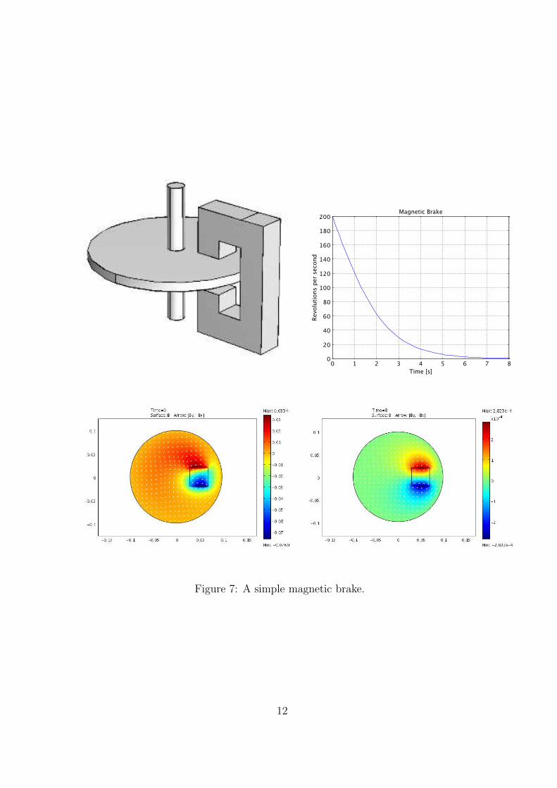
Figure 7: A simple magnetic brake.

12

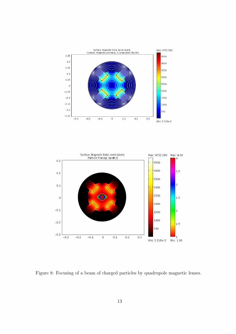
Figure 8: Focusing of a beam of charged particles by quadrupole magnetic lenses.

13

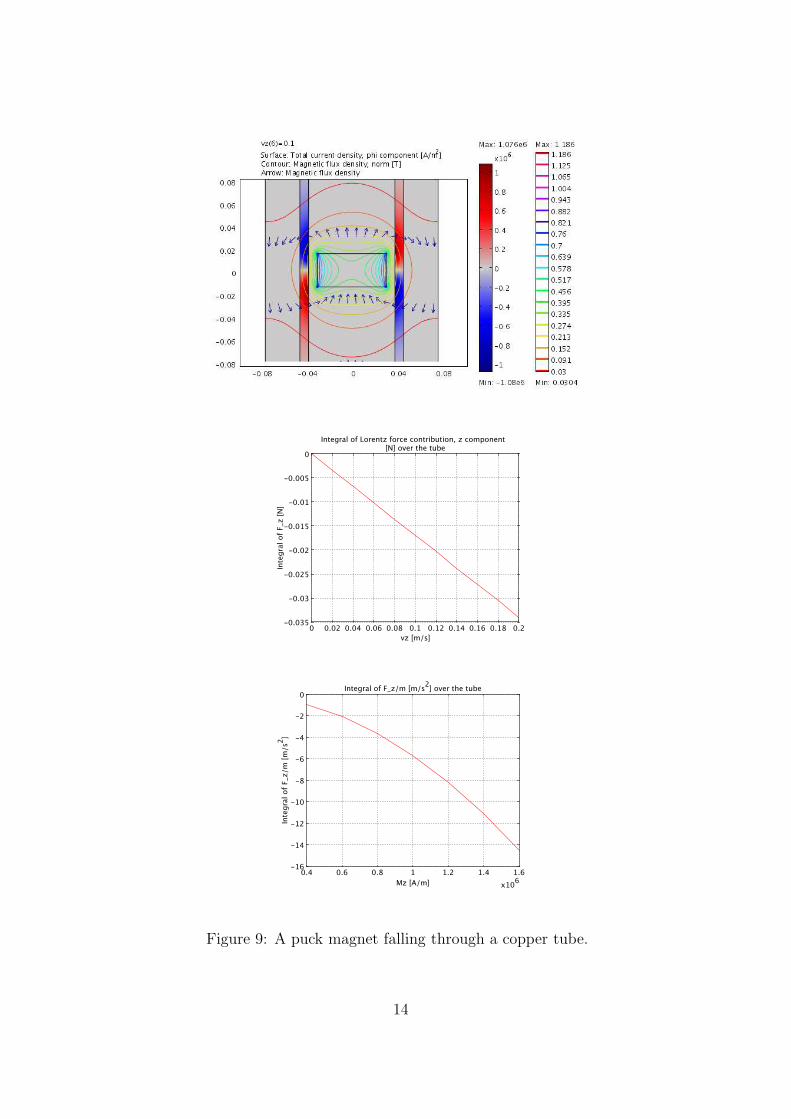
Figure 9: A puck magnet falling through a copper tube.

14