Computing Primer for Applied Linear Regression, Third...

Computing Primerfor

Applied LinearRegression, Third Edition

Using SAS

Keija Shan & Sanford WeisbergUniversity of Minnesota

School of StatisticsAugust 3, 2009

c©2005, Sanford Weisberg

Home Website: www.stat.umn.edu/alr

Contents

Introduction 10.1 Organization of this primer 50.2 Data files 6

0.2.1 Documentation 60.2.2 SAS data library 60.2.3 Getting the data in text files 70.2.4 An exceptional file 7

0.3 Scripts 70.4 The very basics 8

0.4.1 Reading a data file 80.4.2 Saving text output and graphs 90.4.3 Normal, F , t and χ2 tables 9

0.5 Abbreviations to remember 110.6 Copyright and Printing this Primer 11

1 Scatterplots and Regression 131.1 Scatterplots 131.2 Mean functions 181.3 Variance functions 191.4 Summary graph 19

v

vi CONTENTS

1.5 Tools for looking at scatterplots 191.6 Scatterplot matrices 19

2 Simple Linear Regression 232.1 Ordinary least squares estimation 232.2 Least squares criterion 232.3 Estimating σ2 252.4 Properties of least squares estimates 252.5 Estimated variances 252.6 Comparing models: The analysis of variance 252.7 The coefficient of determination, R2 272.8 Confidence intervals and tests 272.9 The Residuals 30

3 Multiple Regression 333.1 Adding a term to a simple linear regression model 333.2 The Multiple Linear Regression Model 343.3 Terms and Predictors 343.4 Ordinary least squares 353.5 The analysis of variance 363.6 Predictions and fitted values 37

4 Drawing Conclusions 394.1 Understanding parameter estimates 39

4.1.1 Rate of change 394.1.2 Sign of estimates 394.1.3 Interpretation depends on other terms in the mean function 394.1.4 Rank deficient and over-parameterized models 39

4.2 Experimentation versus observation 414.3 Sampling from a normal population 414.4 More on R2 414.5 Missing data 414.6 Computationally intensive methods 42

5 Weights, Lack of Fit, and More 455.1 Weighted Least Squares 45

5.1.1 Applications of weighted least squares 465.1.2 Additional comments 47

CONTENTS vii

5.2 Testing for lack of fit, variance known 475.3 Testing for lack of fit, variance unknown 485.4 General F testing 495.5 Joint confidence regions 50

6 Polynomials and Factors 536.1 Polynomial regression 53

6.1.1 Polynomials with several predictors 546.1.2 Using the delta method to estimate a minimum or a maximum 556.1.3 Fractional polynomials 57

6.2 Factors 576.2.1 No other predictors 586.2.2 Adding a predictor: Comparing regression lines 60

6.3 Many factors 616.4 Partial one-dimensional mean functions 616.5 Random coefficient models 63

7 Transformations 677.1 Transformations and scatterplots 67

7.1.1 Power transformations 677.1.2 Transforming only the predictor variable 677.1.3 Transforming the response only 697.1.4 The Box and Cox method 69

7.2 Transformations and scatterplot matrices 717.2.1 The 1D estimation result and linearly related predictors 727.2.2 Automatic choice of transformation of the predictors 72

7.3 Transforming the response 727.4 Transformations of non-positive variables 72

8 Regression Diagnostics: Residuals 738.1 The residuals 73

8.1.1 Difference between e and e 748.1.2 The hat matrix 748.1.3 Residuals and the hat matrix with weights 758.1.4 The residuals when the model is correct 758.1.5 The residuals when the model is not correct 758.1.6 Fuel consumption data 75

8.2 Testing for curvature 76

viii CONTENTS

8.3 Nonconstant variance 778.3.1 Variance Stabilizing Transformations 778.3.2 A diagnostic for nonconstant variance 778.3.3 Additional comments 78

8.4 Graphs for model assessment 788.4.1 Checking mean functions 788.4.2 Checking variance functions 81

9 Outliers and Influence 859.1 Outliers 85

9.1.1 An outlier test 859.1.2 Weighted least squares 859.1.3 Significance levels for the outlier test 859.1.4 Additional comments 86

9.2 Influence of cases 869.2.1 Cook’s distance 879.2.2 Magnitude of Di 889.2.3 Computing Di 889.2.4 Other measures of influence 88

9.3 Normality assumption 88

10 Variable Selection 9110.1 The Active Terms 91

10.1.1 Collinearity 9310.1.2 Collinearity and variances 94

10.2 Variable selection 9410.2.1 Information criteria 9410.2.2 Computationally intensive criteria 9510.2.3 Using subject-matter knowledge 95

10.3 Computational methods 9510.3.1 Subset selection overstates significance 97

10.4 Windmills 9710.4.1 Six mean functions 9710.4.2 A computationally intensive approach 97

11 Nonlinear Regression 9911.1 Estimation for nonlinear mean functions 9911.2 Inference assuming large samples 99

CONTENTS ix

11.3 Bootstrap inference 10511.4 References 106

12 Logistic Regression 10712.1 Binomial Regression 107

12.1.1 Mean Functions for Binomial Regression 10712.2 Fitting Logistic Regression 107

12.2.1 One-predictor example 10812.2.2 Many Terms 10912.2.3 Deviance 11112.2.4 Goodness of Fit Tests 112

12.3 Binomial Random Variables 11312.3.1 Maximum likelihood estimation 11312.3.2 The Log-likelihood for Logistic Regression 113

12.4 Generalized linear models 113

References 115

Index 117

0Introduction

This computer primer supplements the book Applied Linear Regression (alr),third edition, by Sanford Weisberg, published by John Wiley & Sons in 2005.It shows you how to do the analyses discussed in alr using one of severalgeneral-purpose programs that are widely available throughout the world. Allthe programs have capabilities well beyond the uses described here. Differentprograms are likely to suit different users. We expect to update the primerperiodically, so check www.stat.umn.edu/alr to see if you have the most recentversion. The versions are indicated by the date shown on the cover page ofthe primer.

Our purpose is largely limited to using the packages with alr, and we willnot attempt to provide a complete introduction to the packages. If you arenew to the package you are using you will probably need additional referencematerial.

There are a number of methods discussed in alr that are not (as yet)a standard part of statistical analysis, and some methods are not possiblewithout writing your own programs to supplement the package you choose.The exceptions to this rule are R and S-Plus. For these two packages we havewritten functions you can easily download and use for nearly everything in thebook.

Here are the programs for which primers are available.

R is a command line statistical package, which means that the user typesa statement requesting a computation or a graph, and it is executedimmediately. You will be able to use a package of functions for R that

1

2 INTRODUCTION

will let you use all the methods discussed in alr; we used R when writingthe book.

R also has a programming language that allows automating repetitivetasks. R is a favorite program among academic statisticians becauseit is free, works on Windows, Linux/Unix and Macintosh, and can beused in a great variety of problems. There is also a large literaturedeveloping on using R for statistical problems. The main website forR is www.r-project.org. From this website you can get to the page fordownloading R by clicking on the link for CRAN, or, in the US, going tocran.us.r-project.org.

Documentation is available for R on-line, from the website, and in severalbooks. We can strongly recommend two books. The book by Fox (2002)provides a fairly gentle introduction to R with emphasis on regression.We will from time to time make use of some of the functions discussed inFox’s book that are not in the base R program. A more comprehensiveintroduction to R is Venables and Ripley (2002), and we will use thenotation vr[3.1], for example, to refer to Section 3.1 of that book.Venables and Ripley has more computerese than does Fox’s book, butits coverage is greater and you will be able to use this book for more thanlinear regression. Other books on R include Verzani (2005), Maindonaldand Braun (2002), Venables and Smith (2002), and Dalgaard (2002). Weused R Version 2.0.0 on Windows and Linux to write the package. Anew version of R is released twice a year, so the version you use willprobably be newer. If you have a fast internet connection, downloadingand upgrading R is easy, and you should do it regularly.

S-Plus is very similar to R, and most commands that work in R also work inS-Plus. Both are variants of a statistical language called “S” that waswritten at Bell Laboratories before the breakup of AT&T. Unlike R, S-Plus is a commercial product, which means that it is not free, althoughthere is a free student version available at elms03.e-academy.com/splus.The website of the publisher is www.insightful.com/products/splus. Alibrary of functions very similar to those for R is also available that willmake S-Plus useful for all the methods discussed in alr.

S-Plus has a well-developed graphical user interface or GUI. Many newusers of S-Plus are likely to learn to use this program through the GUI,not through the command-line interface. In this primer, however, wemake no use of the GUI.

If you are using S-Plus on a Windows machine, you probably have themanuals that came with the program. If you are using Linux/Unix, youmay not have the manuals. In either case the manuals are availableonline; for Windows see the Help→Online Manuals, and for Linux/Unixuse

> cd ‘Splus SHOME‘/doc

3

Fig. 0.1 SAS windows.

> ls

and see the pdf documents there. Chambers and Hastie (1993) providesthe basics of fitting models with S languages like S-Plus and R. For amore general reference, we again recommend Fox (2002) and Venablesand Ripley (2002), as we did for R. We used S-Plus Version 6.0 Release1 for Linux, and S-Plus 6.2 for Windows. Newer versions of both areavailable.

SAS is the largest and most widely distributed statistical package in bothindustry and education. SAS also has a GUI. When you start SAS,you get the collection of Windows shown in Figure 0.1. While it ispossible to do some data analysis using the SAS GUI, the strength of thisprogram is in the ability to write SAS programs, in the editor window,and then submit them for execution, with output returned in an outputwindow. We will therefore view SAS as a batch system, and concentratemostly on writing SAS commands to be executed. The website for SASis www.sas.com.

4 INTRODUCTION

SAS is very widely documented, including hundreds of books availablethrough amazon.com or from the SAS Institute, and extensive on-linedocumentation. Muller and Fetterman (2003) is dedicated particularlyto regression. We used Version 9.1 for Windows. We find the on-linedocumentation that accompanies the program to be invaluable, althoughlearning to read and understand SAS documentation isn’t easy.

Although SAS is a programming language, adding new functionality canbe very awkward and require long, confusing programs. These programscould, however, be turned into SAS macros that could be reused over andover, so in principle SAS could be made as useful as R or S-Plus. We havenot done this, but would be delighted if readers would take on the chal-lenge of writing macros for methods that are awkward with SAS. Anyonewho takes this challenge can send us the results ([email protected])for inclusion in later revisions of the primer.

We have, however, prepared script files that give the programs that willproduce all the output discussed in this primer; you can get the scriptsfrom www.stat.umn.edu/alr.

JMP is another product of SAS Institute, and was designed around a cleverand useful GUI. A student version of JMP is available. The website iswww.jmp.com. We used JMP Version 5.1 on Windows.

Documentation for the student version of JMP, called JMP-In, comeswith the book written by Sall, Creighton and Lehman (2005), and we willwrite jmp-start[3] for Chapter 3 of that book, or jmp-start[P360] forpage 360. The full version of JMP includes very extensive manuals; themanuals are available on CD only with JMP-In. Fruend, Littell andCreighton (2003) discusses JMP specifically for regression.

JMP has a scripting language that could be used to add functionalityto the program. We have little experience using it, and would be happyto hear from readers on their experience using the scripting language toextend JMP to use some of the methods discussed in alr that are notpossible in JMP without scripting.

SPSS evolved from a batch program to have a very extensive graphical userinterface. In the primer we use only the GUI for SPSS, which limitsthe methods that are available. Like SAS, SPSS has many sophisticatedtools for data base management. A student version is available. Thewebsite for SPSS is www.spss.com. SPSS offers hundreds of pages ofdocumentation, including SPSS (2003), with Chapter 26 dedicated toregression models. In mid-2004, amazon.com listed more than two thou-sand books for which “SPSS” was a keyword. We used SPSS Version12.0 for Windows. A newer version is available.

This is hardly an exhaustive list of programs that could be used for re-gression analysis. If your favorite package is missing, please take this as a

ORGANIZATION OF THIS PRIMER 5

challenge: try to figure out how to do what is suggested in the text, and writeyour own primer! Send us a PDF file ([email protected]) and we will addit to our website, or link to yours.

One program missing from the list of programs for regression analysis isMicrosoft’s spreadsheet program Excel. While a few of the methods describedin the book can be computed or graphed in Excel, most would require greatendurance and patience on the part of the user. There are many add-onstatistics programs for Excel, and one of these may be useful for comprehensiveregression analysis; we don’t know. If something works for you, please let usknow!

A final package for regression that we should mention is called Arc. LikeR, Arc is free software. It is available from www.stat.umn.edu/arc. Like JMPand SPSS it is based around a graphical user interface, so most computationsare done via point-and-click. Arc also includes access to a complete computerlanguage, although the language, lisp, is considerably harder to learn than theS or SAS languages. Arc includes all the methods described in the book. Theuse of Arc is described in Cook and Weisberg (1999), so we will not discuss itfurther here; see also Weisberg (2005).

0.1 ORGANIZATION OF THIS PRIMER

The primer often refers to specific problems or sections in alr using notationlike alr[3.2] or alr[A.5], for a reference to Section 3.2 or Appendix A.5,alr[P3.1] for Problem 3.1, alr[F1.1] for Figure 1.1, alr[E2.6] for an equa-tion and alr[T2.1] for a table. Reference to, for example, “Figure 7.1,” wouldrefer to a figure in this primer, not to alr. Chapters, sections, and homeworkproblems are numbered in this primer as they are in alr. Consequently, thesection headings in primer refers to the material in alr, and not necessarilythe material in the primer. Many of the sections in this primer don’t have anymaterial because that section doesn’t introduce any new issues with regard tocomputing. The index should help you navigate through the primer.

There are four versions of this primer, one for R and S-Plus, and one foreach of the other packages. All versions are available for free as PDF files atwww.stat.umn.edu/alr.

Anything you need to type into the program will always be in this font.Output from a program depends on the program, but should be clear fromcontext. We will write File to suggest selecting the menu called “File,” andTransform→Recode to suggest selecting an item called “Recode” from a menucalled “Transform.” You will sometimes need to push a button in a dialog,and we will write “push ok” to mean “click on the button marked ‘OK’.” Fornon-English versions of some of the programs, the menus may have differentnames, and we apologize in advance for any confusion this causes.

6 INTRODUCTION

Table 0.1 The data file htwt.txt.

Ht Wt

169.6 71.2

166.8 58.2

157.1 56

181.1 64.5

158.4 53

165.6 52.4

166.7 56.8

156.5 49.2

168.1 55.6

165.3 77.8

0.2 DATA FILES

0.2.1 Documentation

Documentation for nearly all of the data files is contained in alr; lookin the index for the first reference to a data file. Separate documenta-tion can be found in the file alr3data.pdf in PDF format at the web sitewww.stat.umn.edu/alr.

The data are available in a package for R, in a library for S-Plus and for SAS,and as a directory of files in special format for JMP and SPSS. In addition,the files are available as plain text files that can be used with these, or anyother, program. Table 0.1 shows a copy of one of the smallest data files calledhtwt.txt, and described in alr[P3.1]. This file has two variables, named Htand Wt, and ten cases, or rows in the data file. The largest file is wm5.txt with62,040 cases and 14 variables. This latter file is so large that it is handleddifferently from the others; see Section 0.2.4.

A few of the data files have missing values, and these are generally indicatedin the file by a place-holder in the place of the missing value. For example, forR and S-Plus, the placeholder is NA, while for SAS it is a period “.” Differentprograms handle missing values a little differently; we will discuss this furtherwhen we get to the first data set with a missing value in Section 4.5.

0.2.2 SAS data library

The data for use with SAS are provided in a special SAS format, or as plaindata files. Instructions for getting and installing the SAS library are given onthe SAS page at www.stat.umn.edu/alr.

If you follow the directions on the web site, you will create a data librarycalled alr3 that will always be present when you start SAS. Most proceduresin SAS have a required data keyword that tells the program where to find thedata to be used. For example, the simple SAS program

proc means data = alr3.heights;

SCRIPTS 7

run;

tells SAS to run the means procedure using the data set heights in the libraryalr3. To run this program, you type it into the editor window, and then selectand submit it; see Section 0.4.1.

0.2.3 Getting the data in text files

You can download the data as a directory of plain text files, or as individualfiles; see www.stat.umn.edu/alr/data. Missing values on these files are indi-cated with a ?. If your program does not use this missing value character, youmay need to substitute a different character using an editor.

0.2.4 An exceptional file

The file wm5.txt is not included in any of the compressed files, or inthe libraries. This one file is nearly five megabytes long, requiring as muchspace as all the other files combined. If you need this file, for alr[P10.12],you can download it separately from www.stat.umn.edu/alr/data.

0.3 SCRIPTS

For R, S-Plus, and SAS, we have prepared script files that can be used whilereading this primer. For R and S-Plus, the scripts will reproduce nearly everycomputation shown in alr; indeed, these scripts were used to do the calcu-lations in the first place. For SAS, the scripts correspond to the discussiongiven in this primer, but will not reproduce everything in alr. The scriptscan be downloaded from www.stat.umn.edu/alr for R, S-Plus or SAS.

Although both JMP and SPSS have scripting or programming languages, wehave not prepared scripts for these programs. Some of the methods discussedin alr are not possible in these programs without the use of scripts, and sowe encourage readers to write scripts in these languages that implement theseideas. Topics that require scripts include bootstrapping and computer inten-sive methods, alr[4.6]; partial one-dimensional models, alr[6.4], inverse re-sponse plots, alr[7.1, 7.3], multivariate Box-Cox transformations, alr[7.2],Yeo-Johnson transformations, alr[7.4], and heteroscedasticity tests, alr[8.3.2].There are several other places where usability could be improved with a script.

If you write scripts you would like to share with others, let me know([email protected]) and I’ll make a link to them or add them to the web-site.

8 INTRODUCTION

0.4 THE VERY BASICS

Before you can begin doing any useful computing, you need to be able to readdata into the program, and after you are done you need to be able to saveand print output and graphs. All the programs are a little different in howthey handle input and output, and we give some of the details here.

0.4.1 Reading a data file

Reading data into a program is surprisingly difficult. We have tried to easethis burden for you, at least when using the data files supplied with alr, byproviding the data in a special format for each of the programs. There willcome a time when you want to analyze real data, and then you will need tobe able to get your data into the program. Here are some hints on how to doit.

SAS If you have created the SAS library called alr3 as suggested in Sec-tion 0.2.2, then all the data files are ready for your use in SAS procedures.For example, the data in htwt.txt is available by referring to the datasetalr3.htwt. If you did not create the library, you can read the data from theplain text files provided into SAS using the menu item File→ Import data file.

If you select this menu item, the SAS import wizard will guide you throughthe process of importing the data. In the first window, select the type of fileyou want to import. If you want to import one of the files supplied with alrsuch as htwt.txt, select “Delimited file (*.*)” from the popup menu. PushNext, and on the next screen browse to find the file on your disk. Use theOptions button on this screen to check the settings for this file. For all thedata files that are provided, the delimiter is a space, the first row of data isrow 2, and “Get variable names from the first row” should be checked. PushNext. On the third screen, you need to assign a name and a library for thisdata set. For example, if you keep the default library work and name the dataset as htwt, then in SAS programs you will refer to this data set as work.htwt.The work library is special because files imported into it are temporary, andwill disappear when you close SAS. If you import the file to any other librarysuch as sasuser, then the file is permanent, and will be available when yourestart SAS.

After selecting a library and name, push Finish. If you push Next, youwill be given the opportunity to save the SAS program generated by the wizardas a file. The code that is saved looks like this:

PROC IMPORT OUT= WORK.htwt

DATAFILE= "z:\working\alr3-data\htwt.txt"

DBMS=DLM REPLACE;

DELIMITER=’20’x;

GETNAMES=YES;

DATAROW=2;

THE VERY BASICS 9

RUN;

Using the wizard is equivalent to writing this SAS program and then executingit. Like most SAS programs: (1) all statements end with a semicolon “;”, (2)the program consists of blocks that begin with a proc to start a procedure andending with a run; to execute it, and (3) several statements are included intothe procedure call, each ending with a semicolon. There are a few exceptionsto these rules that we will encounter later.

SAS is not case-sensitive, meaning that you can type programs in capitals,as shown above, using lower-case letters, or any combination of them youlike.

0.4.2 Saving text output and graphs

All the programs have many ways of saving text output and graphs. We willmake no attempt to be comprehensive here.

SAS Some SAS procedures produce a lot of output. SAS output is by defaultcentered on the page, and assumes that you have paper with 132 columns.You can, however, change these defaults to other values. For example, thefollowing line at the beginning of a SAS program

options nocenter linesize=75 pagesize=66;

will produce left-justified output, assuming 75 columns on a page, and a pagelength of 66 lines.

To save numerical output, click in the output window, and select File→ SaveAs. Alternatively, select the output you want and copy and paste all theoutput to a word processing document or editor. If you use a word processorlike Microsoft Word, be sure to use a monospaced font like Courier New so thecolumns line up properly. To save a graph, click it and then select File→Exportas Image. In the dialog to save the graph, we recommend that you save filesusing “gif” format; otherwise the graphics files will be very large. You canthen print the graph, or import it into a word processing document. We donot recommend copying the graph to the clipboard and pasting it into a wordprocessing document.

0.4.3 Normal, F , t and χ2 tables

alr does not include tables for looking up critical values and significancelevels for standard distributions like the t, F and χ2. Although these valuescan be computed with any of the programs we discuss in the primers, doingso is easy only with R and S-Plus. Also, the computation is fairly easy withMicrosoft Excel. Table 0.2 shows the functions you need using Excel.

SAS SAS allows computing the computing critical values and significancelevels for a very long list of distributions. Two functions are used, called CDF

10 INTRODUCTION

Table 0.2 Functions for computing p-values and critical values using Microsoft Excel.The definitions for these functions are not consistent, sometimes corresponding totwo-tailed tests, sometimes giving upper tails, and sometimes lower tails. Read thedefinitions carefully. The algorithms used to compute probability functions in Excelare of dubious quality, but for the purpose of determining p-values or critical values,they should be adequate; see Knusel (2005) for more discussion.

Function What it does

normsinv(p) Returns a value q such that the area to the left of q fora standard normal random variable is p.

normsdist(q) The area to the left of q. For example, normsdist(1.96)equals 0.975 to three decimals.

tinv(p,df) Returns a value q such that the area to the left of −|q|and the area to the right of +|q| for a t(df) distributionequals q. This gives the critical value for a two-tailedtest.

tdist(q,df,tails) Returns p, the area to the left of q for a t(df) distri-bution if tails = 1, and returns the sum of the areasto the left of −|q| and to the right of +|q| if tails = 2,corresponding to a two-tailed test.

finv(p,df1,df2) Returns a value q such that the area to the right ofq on a F (df1, df2) distribution is p. For example,finv(.05,3,20) returns the 95% point of the F (3, 20)distribution.

fdist(q,df1,df2) Returns p, the area to the right of q on a F (df1, df2)distribution.

chiinv(p,df) Returns a value q such that the area to the right of qon a χ2(df) distribution is p.

chidist(q,df) Returns p, the area to the right of q on a χ2(df) distri-bution.

and quantile. These functions are used inside the data step in SAS, and soyou need to write a short SAS program to get tabled values. For example,the following program returns the p-value from a χ2(25) test with value of thetest statistic equal to 32.5, and also the critical value at the 95% level for thistest.

data qt;

pval = 1-CDF(’chisquare’,32.5,25);

critval = quantile(’chisquare’,.95,25);

output;

proc print data=qt; run;

which returns the output

Obs pval critval

ABBREVIATIONS TO REMEMBER 11

1 0.14405 37.6525

giving the p-value of .14, and the critical value 37.6, for the test.To get F or t significance levels, use functions similar to the following:

1-CDF(’F’,value,df1,df2) F p-valuesquantile(’F’,level,df1,df2) F critical values1-CDF(’t’,value,df) t p-valuesquantile(’t’,level,df) t critical values

For more information, go to Index tab in SAS on-line help, and type eitherquantile or cdf.

0.5 ABBREVIATIONS TO REMEMBER

alr refers to the textbook, Weisberg (2005). vr refers to Venables and Ripley(2002), our primary reference for R and S-Plus. jmp-start refers to Sall,Creighton and Lehman (2005), the primary reference for JMP. Informationtyped by the user looks like this. References to menu items looks like Fileor Transform→Recode. The name of a button to push in a dialog uses thisfont.

0.6 COPYRIGHT AND PRINTING THIS PRIMER

Copyright c© 2005, by Sanford Weisberg. Permission is granted to downloadand print this primer. Bookstores, educational institutions, and instructorsare granted permission to download and print this document for student use.Printed versions of this primer may be sold to students for cost plus a rea-sonable profit. The website reference for this primer is www.stat.umn.edu/alr.Newer versions may be available from time to time.

1Scatterplots and

Regression

1.1 SCATTERPLOTS

A principal tool in regression analysis is the two-dimensional scatterplot. Allstatistical packages can draw these plots. We concentrate mostly on the basicsof drawing the plot. Most programs have options for modifying the appearanceof the plot. For these, you should consult documentation for the program youare using.

SAS Most of the graphics available in SAS are static, meaning that the userwrites a SAS program that will draw the graph, but cannot then interactwith the graph, for example to identify points. The exception is for graphscreated using the Interactive Data Analysis tool obtained by choosing So-lutions→Analysis→ Interactive Data Analysis. We concentrate here on staticgraphics because they are generally drawn using SAS programs. However,since the standard graphing method is first to save the data to be plottedin a data set, and then use proc gplot, one could equally well use anotherprocedure like interactive data analysis for the graphs.

A basic procedure for scatterplots is proc gplot. The following SAS codewill give a graph similar to alr[F1.1] using the heights data:

proc gplot data=alr3.heights;

plot Dheight*Mheight;

run; quit;

As with most SAS examples in this primer, we assume that you have thedata from alr available as a SAS library called alr3; see Section 0.2.2. The

13

14 SCATTERPLOTS AND REGRESSION

Fig. 1.1 SAS version of alr[F1.1] with the heights data.

phrase data=alr3.heights specifies that the data will come from the data setcalled heights in the alr3 library. The phrase plot Dheight*Mheight drawsthe plot with Mheight on the horizontal axis and Dheight on the vertical. run;

tells SAS to execute the procedure, and quit; tells SAS to close the graph,meaning that it will not be enhanced by adding more points or lines. Simplegraphs like this one require only a very short SAS program. The output fromthe above program is shown in Figure 1.1. We saved this file as a PostScriptfile because that is required by our typesetting program. SAS postscript filesseem to be of low quality.

You can also use the menus to draw simple graphs like this one. SelectSolutions→Analyze→ Interactive data analysis, and from in the resulting win-dow, select the library alr3 and the data set heights in that library. The datawill appear in a spreadsheet. Select Analyze→ Scatter plot to draw this plot.An advantage to this method of drawing the plot is that the spreadsheet andthe plot will be linked, meaning that selecting points on the plot will highlightthe corresponding values in the spreadsheet. This can be useful for identifyingunusual points.

Returning to proc gplot, you can add commands that will modify theappearance of the plot. These options must be added before the call to proc

gplot. Continuing with alr[F1.1],

goptions reset=all;

title ’ ’;

symbol v=dot c=black h=.1;

axis1 label=(’Mheight’);

axis2 label=(a=90 ’Dheight’);


plot Dheight*Mheight /haxis=axis1 haxis=55 to 75 hminor=0

SCATTERPLOTS 15

Fig. 1.2 alr[F1.2] with the heights data.

vaxis=axis2 vaxis=55 to 75 vminor=0;

run; quit;

We use the goptions command to reset all options to their default values soleft-over options from a previous graph won’t appear in the current one. Thenext four commands set the title, the plotting symbol, and the labels for thetwo axes. The vertical axis label has been rotated ninety degrees. In in gplot

command, we have specified the haxis and vaxis keywords are set to axis1

and axis2 to get the variable labels. The remainder of the command concernstick marks and to ensure that both axes extended from 55 to 75.

Similar SAS code to produce a version of alr[F1.2] illustrates using thewhere statement:

goptions reset=all;


plot Dheight*Mheight /haxis=axis1 haxis=55 to 75 hminor=0

vaxis=axis2 vaxis=55 to 75 vminor=0;

where (Mheight ge 57.5) & (Mheight le 58.5) |

(Mheight ge 62.5) & (Mheight le 63.5) |

(Mheight ge 67.5) & (Mheight le 68.5);

run; quit;

Inside proc gplot, specify the data set by data=dataset-name. The first ar-gument Dheight will be the vertical axis variable, and the second argumentMheight will be on the horizontal axis. As with many SAS commands, optionsfor a command like plot are added after a /. We let the horizontal axis beaxis1, and the vertical axis be axis2. The where statement uses syntax similarto the C language. The logical operators & for and and | for or are used tospecify ranges for plotting.


a. (a) ols prediction. b. (b) ols residual plot.

Fig. 1.3 SAS version of alr[F1.3]. (sassupp104)

A few reminders:

1. All statements end with ;.

2. Always use goptions reset=all; to remove all existing graphical setupbefore plotting.

3. Statements for changing graphical options like symbol have to be speci-fied before proc gplot is called.

4. Nearly all SAS commands end with run;.

alr[F1.3-1.4] includes both points and fitted lines. For alr[F1.3a], weneed to get the ols fitted line. For alr[F1.3b], we need to compute residuals.This can be done by calling proc reg in SAS, which also allows graphing:

goptions reset=all;

symbol v=circle h=1;

proc reg data=alr3.forbes;

model Pressure=Temp;

plot Pressure*Temp;

plot residual.*Temp;

run;

We define circle as the plotting symbol in the symbol statement. For the model

statement, the syntax is model response=terms;. The plot command in proc

reg draws graphs of regression quantities, with the syntax horizontal*vertical.With simple regression, the plot of the response versus the single predictoradds the ols line automatically. The second plot makes use of the keywordresidual. to get the residuals. Do not forget the dot after keywords!

alr[F1.5] includes both an ols line and a line that joins the mean lengthsat each age. Although this plot seems simple, the SAS program we wrote to

SCATTERPLOTS 17

obtain it is surprisingly difficult and not particularly intuitive. Here is theSAS, program:

proc loess data=alr3.wblake;

model Length=Age /smooth=.1;

ods output OutputStatistics=m1;

run;

proc reg data=alr3.wblake;

model Length=Age;

output out=m2 pred=ols;

run;

data m3; set alr3.wblake; set m1; set m2;

proc sort data=m3; by Age;

goptions reset=all;

symbol1 v=circle h=1 c=black l=1 i=join;

symbol2 v=circle h=1 c=black l=2 i=join;

symbol3 v=circle h=1 c=black;

axis2 label=(a=90 ’Length’);

proc gplot data=m3;

plot ols*Age=1 Pred*Age=2 Length*Age=3

/overlay hminor=0 vaxis=axis2 vminor=0;

run; quit;

The plot consists of three parts: the points, the ols fitted line, and the linejoining the means for each value of Age. We couldn’t think of obvious wayto get this last line, and so we used a trick. The loess smoother, discussed inalr[A.5], can be used for this purpose by setting the smoothing parameter tobe a very small number, like .1. The call shown to proc loess will compute themean Length for each Age called m1. Confusingly, you use an ods statement,not output, to save the output from proc lowess. Next, proc reg is used toget the regression of Length on Age. The output is saved using the output

statement, not ods. This output includes the input data and the predictedvalues in a new data set called m2.

We now have the information for joining the points in the data set m1

and the data for fitting ols in m2. The data statement combines them withalr3.wblake in another data set called m3. A few graphics commands arethen used. The , symbol2 and symbol3 define plotting symbols; you can definesymbol4, symbol5 and so on. The option i=join tells SAS to connect the pointsusing straight lines. The option l=1 refers to a connection with solid line, andl=2 refers to a connection with a dashed line. proc sort was used to arrangethe data set by an ascending order (which is the default) of variable Age. Thismakes sure that we do not get a mess when we connect data points to get theols line. After we customize each symbol, we can write ols*Age=1 Pred*Age=2

Length*Age=3 in the plot statement, which simply means that use the firstcustomized symbol for the plot of ols versus Age, the second customized symbol

for the plot of loess Pred versus Age, and the third customized symbol for thescatterplot of Length versus Age. proc gplot was called with the data set m3.The overlay option further modifies the axes of the plot.


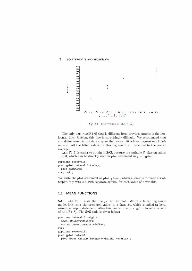
Fig. 1.4 SAS version of alr[F1.7].

The only part alr[F1.6] that is different from previous graphs is the hor-izontal line. Getting this line is surprisingly difficult. We recommend thatyou define one=1 in the data step so that we can fit a linear regression of Lateon one. All the fitted values for this regression will be equal to the overallaverage.

alr[F1.7] is easier to obtain in SAS, because the variable S takes on values1, 2, 3, which can be directly used in plot statement in proc gplot:

goptions reset=all;

proc gplot data=alr3.turkey;

plot gain*A=S;

run; quit;

We write the plot statement as plot y*x=z;, which allows us to make a scat-terplot of y versus x with separate symbol for each value of z variable.

1.2 MEAN FUNCTIONS

SAS alr[F1.8] adds the line y=x to the plot. We fit a linear regressionmodel first, save the predicted values to a data set, which is called m1 here,using the output statement. After this, we call the proc gplot to get a versionof alr[F1.8]. The SAS code is given below:

proc reg data=alr3.heights;

model Dheight=Mheight;

output out=m1 predicted=Dhat;

run;

goptions reset=all;

proc gplot data=m1;

plot (Dhat Mheight Dheight)*Mheight /overlay ;

VARIANCE FUNCTIONS 19

run; quit;

1.3 VARIANCE FUNCTIONS

1.4 SUMMARY GRAPH

1.5 TOOLS FOR LOOKING AT SCATTERPLOTS

SAS proc loess can be used to add a loess smoother to a graph. The fol-lowing produces a version of alr[F1.10]:

proc reg data=alr3.heights;


output out=m1 predicted=Dhat;

run;

proc loess data=alr3.heights;

model Dheight=Mheight /smooth=.6;

ods output OutputStatistics=myout;

run;

data myout; set myout; set m1;

proc sort data=myout; by Mheight; run;

goptions reset=all;

proc gplot data=myout;

plot (Dhat Pred DepVar)*Mheight /overlay;

run; quit;

This procedure produces loess estimates given a smoothing parameter, whichis 0.6 here (specified using smooth). The smoothing parameter must be strictlypositive and less than one. The statement ods output is used to produceprocedure-specific output. We have saved the output in a data set calledmyout. After combining myout from proc loess and the output m1 from olsfit, we sort the data by Mheight, the variable to be plotted on the horizontalaxis. As we have mentioned before, this is simply for visual clarification sincewe are going to connect the loess estimates to get a loess curve. DepVar is justthe dependent variable Dheight, in a different name in the output data myout.Pred is the loess estimate. The quit; statement stops procedures called beforeit.

1.6 SCATTERPLOT MATRICES

SAS This is the first example we have encountered that requires transfor-mation of some of the variables to be graphed. This is done by creating a newdata set that consists of the old variables plus the transformed variables. Thedata step in SAS for transformations.


Fig. 1.5 SAS version of alr[F1.10].

Scatterplot matrices are obtained using proc insight. For the fuel2001

data, here is the program:

data m1;

set alr3.fuel2001;

Dlic=Drivers*1000/Pop;

Fuel=FuelC*1000/Pop;

logMiles=log2(Miles);

goptions reset=all;

proc insight data=m1;

scatter Tax Dlic income logMiles Fuel

*Tax Dlic income logMiles Fuel;

run;

In the data step, we created a new data set called m1 that includes all ofalr3.fuel2001 from the set statement, and the three additional variables com-puted from transformations; note the use of log2 for base-two logarithms. Wecalled proc insight using this new data set.

Solutions→Analysis→ Interactive Data Analysis also starts proc insight.You can also transform variables from within this procedure.

Graphs created with proc insight are interactive. If you click the mouseon a point in this graph, the point will he highlighted in all frames of thescatterplot matrix, and its case number will be displayed on the graph.

SCATTERPLOT MATRICES 21

Fig. 1.6 SAS scatterplot matrix for the fuel2001 data.

Problems

1.1. Boxplots would be useful in a problem like this because they display level(median) and variability (distance between the quartiles) simultaneously.

SAS SAS has a proc boxplot procedure. You can follow the generic syntaxas follows:

proc boxplot data=alr3.wblake;

plot Length*Age;

run;

The above SAS code means that a separate boxplot of Length will be providedat each value of Age.

As an alternative, you can use the SAS Interactive Data Analysis toolto obtain boxplots. After you launch it with a data set, you can chooseAnalyze→Box Plot/Mosaic Plot(Y) from the menu. Then you click on Lengthonce and click the Y button once. Similarly, you can move the variable Age tothe box under the X button. After you click the OK button, a series of boxplotsof Length for each value of Age are printed on the screen.


Just a reminder: Even if you choose to use SAS Interactive Data Analysistool, you must have the data available in advance, either using a SAS datastep, or using a data file from a library.

To get the standard deviation at each value of Age, you can call proc means

or proc summary (which is exactly the same as proc means except that it doesnot show output) and put Age in the class statement. The keyword forretrieving standard deviation is std.1.2.

SAS To change the size of an image in SAS, you can move you mouse cursorto the right-bottom edge of the graph window. When the cursor becomes adouble arrow, click and hold the left button of your mouse, then drag the edgeto any size.1.3.

SAS In SAS, log2(Fertility) returns the base-two logarithms. If you needtransformations, use the procedure outlined in Section 1.6 of the primer.

2Simple Linear Regression

2.1 ORDINARY LEAST SQUARES ESTIMATION

All the computations for simple regression depend on only a few summarystatistics; the formulas are given in the text, and in this section we show howto do the computations step–by-step. All computer packages will do thesecomputations automatically, as we show in Section 2.6.

2.2 LEAST SQUARES CRITERION

SAS The procedure proc means can be used to get summary statsitics; seeTable 2.1.

proc means data=alr3.forbes;

var Temp Lpres;

run;

Table 2.1 proc means output with the forbes data.

The MEANS Procedure

Variable N Mean Std Dev Minimum Maximum

Temp 17 202.9529412 5.7596786 194.3000000 212.2000000

Lpres 17 139.6052941 5.1707955 131.7900000 147.8000000

23

24 SIMPLE LINEAR REGRESSION

This chapter illustrates the computations that are usually hidden by regres-sion programs. You can follow along with the calculations with the interactivematrix language in SAS, called proc iml.

data f;

set alr3.forbes ;

one=1;

proc iml;

use f;

read all var {one Temp Pressure Lpres}

where (Temp^=. & Pressure^=. & Lpres^=.) into X;

size=nrow(X); W=X‘*X;

Tempbar=W[1,2]/size; Lpresbar=W[1,4]/size; Y=j(size,2,0);

Y[,1]=X[,2]-Tempbar; Y[,2]=X[,4]-Lpresbar;

fcov=Y‘*Y; RSS=fcov[2,2]-fcov[1,2]**2/fcov[1,1];

sigmahat2=RSS/(size-2); sigmahat=sqrt(sigmahat2);

b1=fcov[1,2]/fcov[1,1];

b0=Lpresbar-b1*Tempbar;

title ’PROC IML results’;

print Tempbar Lpresbar fcov b1 b0 RSS sigmahat2;

create forbes_stat var{Tempbar Lpresbar fcov b1 b0 RSS sigmahat2};

append var{Tempbar Lpresbar fcov b1 b0 RSS sigmahat2};

close forbes_stat;

quit;

Table 2.2 proc iml results with the forbes data.

PROC IML results

TEMPBAR LPRESBAR FCOV B1 B0 RSS SIGMAHAT2

202.95294 139.60529 530.78235 475.31224 0.8954937 -42.13778

2.1549273 0.1436618

475.31224 427.79402

We start by creating a new data set called f that has all the variables inalr3.forbes plus a new variable called one that repeats the value 1 for allcases in the data set, so it is a vector of length 17.

The keywords used in proc iml include use, read all var, where and into.These load all the variables of interest into the procedure so that we can com-pute various summary statistics. The variables in the braces are collected intoa new matrix variable we called X , whose columns represent the variables inthe order they are entered. The where statement guarantees that all calcu-lations will be done on non-missing values only. “^=” stands for “not equalto”, and is equivalent to the operator ne (not equal) outside proc iml. Theoperator X‘*X denotes a matrix product X ′X . Use the single-quote located atthe upper left corner of the computer keyboard, not the usual one, to denotethe transpose. An alternative way of specifying the transpose of a matrix Xis by t(X). The function j(size,2,0) creates a matrix of dimension size by 2

ESTIMATING σ2 25

of all zeroes. The operator “**2” is for exponentiating, here squaring. Theprint statement asks SAS to display some results, and the create and append

statements save some of the variables into a data set called forbes stat. Thecreate statement defines a structure of the data set called forbes stat, andthe append statement fills in values. If some variables do not have the samelength, then “.” will be used in the new data set for missing values. The close

statement simply denotes closing the data set.The SAS code gives the sample means, the sample covariance matrix, re-

gression coefficient estimates, RSS and variance estimate; see Table 2.2.

2.3 ESTIMATING σ2

SAS From proc iml, we can easily get the variance estimate as sigmahat2

in the output of proc iml above. RSS is also given above from proc iml. Seethe last section.

2.4 PROPERTIES OF LEAST SQUARES ESTIMATES

2.5 ESTIMATED VARIANCES

The estimated variances of coefficient estimates are computed using the sum-mary statistics we have already obtained. These will also be computed auto-matically linear regression fitting methods, as shown in the next section.

2.6 COMPARING MODELS: THE ANALYSIS OF VARIANCE

Computing the analysis of variance and F test by hand requires only the valueof RSS and of SSreg = SYY − RSS. We can then follow the outline given inalr[2.6].

SAS There are several SAS procedures that can do simple linear regression.The most basic procedure is proc reg, which prints at minimum the summaryof the fit and the ANOVA table. For the Forbes data,

proc reg data = alr3.forbes;

model Lpres = Temp;

run;

is the smallest program for fitting regression. This will give the output shownin Table 2.3.

There are literally dozens of options you can add to the model statementthat will modify output. For example, consider the following five statements:

model Lpres=Temp;


Table 2.3 Output of proc reg with the forbes data.

The REG Procedure

Model: MODEL1

Dependent Variable: Lpres

Analysis of Variance

Sum of Mean

Source DF Squares Square F Value Pr > F

Model 1 425.63910 425.63910 2962.79 <.0001

Error 15 2.15493 0.14366

Corrected Total 16 427.79402

Root MSE 0.37903 R-Square 0.9950

Dependent Mean 139.60529 Adj R-Sq 0.9946

Coeff Var 0.27150

Parameter Estimates

Parameter Standard

Variable DF Estimate Error t Value Pr > |t|

Intercept 1 -42.13778 3.34020 -12.62 <.0001

Temp 1 0.89549 0.01645 54.43 <.0001

model Lpres=Temp/noprint;

model Lpres=Temp/noint;

model Lpres=Temp/all;

model Lpres=Temp/CLB XPX I R;

All but the third will fit the same regression, but will differ on what is printed.The first will print the default output in Table 2.3. The second will produceno printed output, and is useful if followed by an output statement to saveregression summaries for some other purpose. The third will fit a mean func-tion with no intercept. The fourth will produce pages and pages of output,of everything the program knows about; you probably don’t want to use thisoption very often (or ever). The last will print the default output confidenceintervals for each of the regression coefficients, the matrix X ′X , its inverse(X ′X)−1, and a printed version of the residuals. See documentation for proc

reg for a complete list of options.Remember that transformations must be done in a data step, not in proc

reg.proc glm Another important SAS procedure for fitting linear models is

proc glm, which stands for the general linear model. proc glm is is moregeneral than proc reg because it allows class variables, which is the namethat SAS uses for factors. Also, proc glm has several different approachesto fitting ANOVA tables. The approach to ANOVA discussed in alr[3.5] issequential ANOVA, called Type I in SAS. The Wald or t-tests discussed inalr are equivalent to SAS Type II, with no factors present. SAS Type III is

THE COEFFICIENT OF DETERMINATION, R2 27

not recommended in any regression problem. Table 2.4 gives a comparison ofproc reg and proc glm.

2.7 THE COEFFICIENT OF DETERMINATION, R2

2.8 CONFIDENCE INTERVALS AND TESTS

Confidence intervals and tests can be computed using the formulas in alr[2.8],in much the same way as the previous computations were done.

SAS The SAS procedure proc reg will give confidence intervals for parame-ter estimates by adding the option clb to the model statement, so, for example,

model Lpres=Temp/clb alpha=.01;

will print 99% confidence intervals; the default is 95% intervals.A function called tinv(p,df) can be used in a data step to calculate quan-

tiles for t-distribution with df degrees of freedom. Similar functions includebetainv(p,a,b) for Beta distribution, cinv(p,df) for χ2 distribution, gaminv(p,a)for Gamma distribution, finv(p,ndf,ddf) for F -distribution, and probit(p)

for standard normal distribution. All of these functions can be used in thedata step or any SAS procedure.

Prediction and fitted values

SAS It is easy in SAS to get fitted values and associated confidence intervalsfor each observation by adding the option cli keyword to the model statementin proc reg:

proc reg data=alr3.forbes alpha=.05;

model Lpres=Temp /cli;

run;

To get predictions and confidence intervals at unobserved values of the predic-tors, you need to append new data to the data set, with a missing indicator (aperiod) for the response. In the Forbes data, for example, to get predictionsat Temp = 210, 200, use

data forbes2;

input Temp;

cards;

210

220

;

data forbes2;

set alr3.forbes forbes2;

proc reg data=forbes2 alpha=.05;


Table 2.4 Comparison of proc reg and proc glm.

Property proc reg proc glm

Terms

Class variables (called fac-tors in alr)

Not allowed; use dummyvariables instead

Allowed

Polynomial terms and in-teractions

Not allowed; define them indata step

Allowed

Other transformations Use a data step Use a data stepRandom effects Not allowed Not recommended; use

proc mixed instead.

Fitting

ols and wls Yes YesNo intercept Allowed Allowed

Prediction/Fitted values

Prediction at new values Add new values for thepredictors to the data setwith missing values, indi-cated by a “.”, for the re-sponse.

Allowed

Miscellaneous

Covariance of estimates Yes No; but can be com-puted from model out-put

ANOVA tables Overall ANOVA only. Overall and sequentialANOVA and othertypes of SS, reallydifferent orders offitting

R2 Yes YesAdd/delete variables andrefit

Allowed Not allowed

Submodel selection Allowed Not allowed

Model diagnostics

Diagnostic statistics Yes YesGraphical diagnostics Yes No

CONFIDENCE INTERVALS AND TESTS 29

model Lpres=Temp /cli;

run;

Table 2.5 Predictions and prediction standard errors for the forbes data.

The REG Procedure

Model: MODEL1

Dependent Variable: Lpres

Output Statistics

Dep Var Predicted Std Error

Obs Lpres Value Mean Predict 95% CL Predict Residual

1 131.7900 132.0357 0.1667 131.1532 132.9183 -0.2457

2 131.7900 131.8566 0.1695 130.9717 132.7416 -0.0666

3 135.0200 135.0804 0.1239 134.2304 135.9304 -0.0604

4 135.5500 135.5282 0.1186 134.6817 136.3747 0.0218

5 136.4600 136.4237 0.1089 135.5831 137.2642 0.0363

6 136.8300 136.8714 0.1048 136.0332 137.7096 -0.0414

7 137.8200 137.7669 0.0979 136.9325 138.6013 0.0531

8 138.0000 137.9460 0.0969 137.1122 138.7798 0.0540

9 138.0600 138.2146 0.0954 137.3816 139.0477 -0.1546

10 138.0400 138.1251 0.0959 137.2918 138.9584 -0.0851

11 140.0400 140.1847 0.0925 139.3531 141.0163 -0.1447

12 142.4400 141.0802 0.0958 140.2469 141.9135 1.3598

13 145.4700 145.4681 0.1416 144.6057 146.3306 0.001856

14 144.3400 144.6622 0.1307 143.8076 145.5168 -0.3222

15 146.3000 146.5427 0.1571 145.6682 147.4173 -0.2427

16 147.5400 147.6173 0.1735 146.7288 148.5059 -0.0773

17 147.8000 147.8860 0.1777 146.9937 148.7783 -0.0860

18 . 145.9159 0.1480 145.0486 146.7831 .

19 . 154.8708 0.2951 153.8469 155.8947 .

Sum of Residuals -3.3378E-13

Sum of Squared Residuals 2.15493

Predicted Residual SS (PRESS) 2.52585

The new data for the input variable Temp are entered after the cards state-ment; we need to use the same variable name as in the forbes data set so thatthese new values will be appended to the column of our interest.

To save the predicted values and associated confidence intervals for latercomputation, you can use output statement in proc reg. Here the informationis saved to a data set called m1:

data forbes2;

input Temp;

cards;

210

220

;

data forbes2;

set alr3.forbes forbes2;


proc reg data=forbes2 alpha=.05;

model Lpres=Temp /cli noprint;

output out=m1 predicted=prediction L95=Lower_limit U95=Upper_limit;

run;

2.9 THE RESIDUALS

SAS The SAS procedure proc reg computes the residuals for the linearmodel we fit. A plot of residuals versus fitted values can be obtained usingplot statement in proc reg. The keywords are residual., the ordinary resid-uals, and predicted.; don’t forget the trailing periods. The /nostat nomodel

option suppresses the model fit information on the graph.

proc reg data=alr3.forbes;

model Lpres=Temp /noprint;

output out=m1 residual=res predicted=pred;

plot residual.*predicted. /nostat nomodel; *the residual plot;

run;

proc print data=work.m1 ;

run;

The output statement was used to save the residuals and fitted values in adata set called m1. We then used proc print to print m1, but you could usethis data set in other graphs or for other purposes.

Problems

2.2.

SAS In order to do part 2.2.3, you need to save the fitted values from thetwo regression models to two data sets, then apply SAS graphical procedureto the combined data set.

For part 2.2.5, you also need to save the predicted values and predictionstandard errors, then use a data step to combine these data and the Hooker’sdata.

For part 2.2.6, you first need to combine the forbes data and the Hooker’sdata, with the response in the forbes data to missing. Then you fit theregression model with this combined data set. Since SAS provides predictionsfor the data with missing response as well, the computation of z-scores arestill straightforward in this part.2.7.

SAS A linear regression model without an intercept can be fit in SAS byadding noint option to the model statement.2.10.

THE RESIDUALS 31

SAS The where conditions; statement can be used to select the cases ofinterest.

3Multiple Regression

3.1 ADDING A TERM TO A SIMPLE LINEAR REGRESSION MODEL

SAS Using the fuel2001 data, we first need to transform variables and createa new data set that includes them. To draw an added-variable plot in SAS,we use proc reg twice to get the sets of residuals that are needed. Using thefuel2001 data,

data fuel;

set alr3.fuel2001;



Income=Income/1000;


goptions reset=all;

title ’Added Variable Plot for Tax’;

proc reg data=fuel;

model Fuel Tax=Dlic Income logMiles;

output out=m1 residual=res1 res2;

run;

proc reg data=m1;

model res1=res2;

plot res1*res2;

run;

The first proc reg has a model statement with two responses on the left sideof the equal sign. This means that two regression models will be fit, onefor each response. The output specification assigns m1 to be the name of the

33

34 MULTIPLE REGRESSION

Table 3.1 Summary statistics from proc means for the fuel2001 data.

The MEANS Procedure

Variable N Mean Std Dev Minimum Maximum

Tax 51 20.1549020 4.5447360 7.5000000 29.0000000

Dlic 51 903.6778311 72.8578005 700.1952729 1075.29

Income 51 28.4039020 4.4516372 20.9930000 40.6400000

logMiles 51 15.7451611 1.4867142 10.5830828 18.1982868

Fuel 51 613.1288080 88.9599980 317.4923972 842.7917524

output, and the names for the two sets of residuals are res1 and res2. Theadded-variable plot is just the plot of res1 versus res2. We did this using plot

inside the next proc reg; in this way, the fitted line and summary statisticsare automatically added to the plot.

A low-quality version of all the added-variable plots (produced in the out-put window rather than a graphics window) can be produced using the partial

option:

data=fuel;

model Fuel = Tax Dlic Income logMiles/partial;

run;

A synonym for an added-variable plot is a partial regression plot.

3.2 THE MULTIPLE LINEAR REGRESSION MODEL

3.3 TERMS AND PREDICTORS

SAS The standard summary statistics in SAS can be retrieved using proc

means, and the output is in Table 3.1.

data fuel;

set alr3.fuel2001;



Income=Income/1000;


proc means data=fuel;

var Tax Dlic Income logMiles Fuel;

run;

We will use proc iml, the interactive matrix language that we used in thelast chapter, for several calculations and covariances. First, we get the samplecorrelations, starting with the fuel data set that we have just created.

proc iml;

use fuel;

ORDINARY LEAST SQUARES 35

read all var {Tax Dlic Income logMiles Fuel} into X;

size=nrow(X); one=j(1,size,1);

ave=one*X/size;

Xave=one‘*ave;

W=X-Xave; Y=W‘*W;

Xcov=Y/(size-1);

Xstd=sqrt(diag(Xcov)); Xstd_inv=inv(Xstd);

Xcor=Xstd_inv*Xcov*Xstd_inv;

print Xcor Xcov;

quit;

We have used inv to get the inverse of a matrix; it is equivalent to X‘. Seeoutput in Table 3.2.

Table 3.2 Sample correlation matrix and sample covariance matrix from proc iml

for the fuel2001 data.

XCOR

1 -0.085844 -0.010685 -0.043737 -0.259447

-0.085844 1 -0.175961 0.0305907 0.4685063

-0.010685 -0.175961 1 -0.295851 -0.464405

-0.043737 0.0305907 -0.295851 1 0.4220323

-0.259447 0.4685063 -0.464405 0.4220323 1

XCOV

20.654625 -28.4247 -0.216173 -0.295519 -104.8944

-28.4247 5308.2591 -57.07045 3.3135435 3036.5905

-0.216173 -57.07045 19.817074 -1.958037 -183.9126

-0.295519 3.3135435 -1.958037 2.2103191 55.817191

-104.8944 3036.5905 -183.9126 55.817191 7913.8812

3.4 ORDINARY LEAST SQUARES

SAS Continuing with using proc iml to do matrix calculations, the ols es-timates can be computed from (X ′X)−1X ′Y ; results are shown in Table 3.3.

data fuel;

set alr3.fuel;



Income=Income/1000;


one=1;

proc iml;

use fuel2001;

read all var {one Tax Dlic Income logMiles} where (one^=. &

Tax^=. & Dlic^=. & Income^=. & logMiles^=. & fuel^=.) into X;

read all var ’fuel’ where (one^=. &


Tax^=. & Dlic^=. & Income^=. & logMiles^=. & fuel^=.) into Y;

beta_hat=inv(t(X)*X)*t(X)*Y;

print beta_hat;

quit;

Table 3.3 ols using proc iml for the fuel2001 data.

BETA_HAT

154.19284

-4.227983

0.4718712

-6.135331

18.545275

The ols estimates can be obtained using proc reg or proc glm. The outputfrom proc glm is given in Table 3.4. The syntax is very similar to that forsimple linear regression.

proc glm data=fuel;

model Fuel=Tax Dlic Income logMiles;

run;

The only difference between fitting simple and multiple regression is in thespecification of the model. All terms in the mean function appear to the rightof the equal sign, separated by white space. The output for using proc reg

would be similar, but would not include the extensive ANOVA tables shown.

3.5 THE ANALYSIS OF VARIANCE

SAS We recommend using proc glm for getting sequential analysis variancetables. For example,

proc glm data=fuel;

model Fuel=Tax Dlic Income logMiles/ss1;

run;

produces the output shown in Table 3.4. This output gives the overall ANOVA,and by the sequential ANOVA discussed in alr, and called Type I ANOVA bySAS. By using the option /ss1, we have suppressed SAS’s default behavior ofprinting what it calls “Type III” sums of squares; these are not recommended(Nelder, 1977).

The order of fitting is determined by the order of the terms in the model

statement. Thus

proc glm data=fuel;

model Fuel=logMiles Income Tax Dlic /ss1;

run;

would fit logMiles first, then Income, Tax and finally Dlic.

PREDICTIONS AND FITTED VALUES 37

Table 3.4 Anova for nested models in proc reg for the fuel2001 data.

The GLM Procedure

Dependent Variable: Fuel

Sum of

Source DF Squares Mean Square F Value Pr > F

Model 4 201994.0473 50498.5118 11.99 <.0001

Error 46 193700.0152 4210.8699


R-Square Coeff Var Root MSE Fuel Mean

0.510480 10.58362 64.89122 613.1288

Source DF Type I SS Mean Square F Value Pr > F

Tax 1 26635.27578 26635.27578 6.33 0.0155

Dlic 1 79377.52778 79377.52778 18.85 <.0001

Income 1 61408.17553 61408.17553 14.58 0.0004

logMiles 1 34573.06818 34573.06818 8.21 0.0063

Standard

Parameter Estimate Error t Value Pr > |t|

Intercept 154.1928446 194.9061606 0.79 0.4329

Tax -4.2279832 2.0301211 -2.08 0.0429

Dlic 0.4718712 0.1285134 3.67 0.0006

Income -6.1353310 2.1936336 -2.80 0.0075

logMiles 18.5452745 6.4721745 2.87 0.0063

3.6 PREDICTIONS AND FITTED VALUES

SAS As with simple regression, we get predictions and prediction intervalsby appending new data points to the data set with missing values for theresponse. See output in Table 3.5.

data fuel2;

input Tax Dlic Income logMiles;

cards;

20 909 16.3 626

35 943 16.8 667

;

data fuel2; set fuel fuel2;

proc reg data=fuel2 alpha=.05;

model Fuel=Tax Dlic Income logMiles /cli;

run;

We created a data file called fuel2 consisting of two cases with values for fourvariables. We then redefined fule2 by appending it to the bottom of fuel; all


Table 3.5 Predictions and prediction standard errors at new values from proc reg

for the fuel2001 data.

The REG Procedure

Model: MODEL1

Dependent Variable: Fuel

... ... (omitted)

Output Statistics

Dep Var Predicted Std Error

Obs Fuel Value Mean Predict 95% CL Predict Residual

1 690.2644 727.2652 20.2801 590.4156 864.1147 -37.0007

2 514.2792 677.4242 32.8388 531.0318 823.8166 -163.1450

... ... (omitted)

50 581.7937 593.1223 18.5974 457.2446 729.0000 -11.3286

51 842.7918 659.2930 18.7829 523.3120 795.2740 183.4988

52 . 12008 3942 4072 19944 .

53 . 12718 4209 4244 21192 .

... ... (omitted)

other variables are missing for these two cases. We then fit the regression,and obtain predictors for the two added cases.

Problems

4Drawing Conclusions

The first three sections of this chapter do not introduce any new computationalmethods; everything you need is based on what has been covered in previouschapters. The last two sections, on missing data and on computationallyintensive methods introduce new computing issues.

4.1 UNDERSTANDING PARAMETER ESTIMATES

4.1.1 Rate of change

4.1.2 Sign of estimates

4.1.3 Interpretation depends on other terms in the mean function

4.1.4 Rank deficient and over-parameterized models

SAS SAS provides several diagnostics when you try to fit a mean functionin which some terms are linear combinations of others. Table 4.1 provides theoutput that parallels the discussion in alr[4.1.4].

data BGS;

set alr3.BGSgirls;

DW9=WT9-WT2;

DW18=WT18-WT9;

proc reg data=BGS;

model Soma=WT2 DW9 DW18 WT9 WT18;

run;

39

40 DRAWING CONCLUSIONS

Table 4.1 Output from an over-parameterized model for the BGSgirls data.

The REG Procedure

Model: MODEL1

Dependent Variable: SOMA

Number of Observations Read 70

Number of Observations Used 70

Analysis of Variance

Sum of Mean

Source DF Squares Square F Value Pr > F

Model 3 25.35982 8.45327 28.67 <.0001

Error 66 19.45803 0.29482


Root MSE 0.54297 R-Square 0.5658

Dependent Mean 4.77857 Adj R-Sq 0.5461

Coeff Var 11.36264

NOTE: Model is not full rank. Least-squares solutions for the

parameters are not unique. Some statistics will be misleading.

A reported DF of 0 or B means that the estimate is biased.

NOTE: The following parameters have been set to 0, since the

variables are a linear combination of other variables as shown.

WT9 = WT2 + DW9

WT18 = WT2 + DW9 + DW18

Parameter Estimates

Parameter Standard

Variable DF Estimate Error t Value Pr > |t|

Intercept 1 1.59210 0.67425 2.36 0.0212

WT2 B -0.01106 0.05194 -0.21 0.8321

DW9 B 0.10459 0.01570 6.66 <.0001

DW18 B 0.04834 0.01060 4.56 <.0001

WT9 0 0 . . .

WT18 0 0 . . .

Besides providing the correct ANOVA and other estimates, SAS correctlyreports the linear combinations of the terms in the mean function. It thengives the estimates of parameters in the manner suggested in the text, bydeleting additional terms that are exact linear combinations of previous termsin the mean function. SAS reports “B” degrees of freedom for the terms fitthat are part of the exact linear combinations to indicate that the fit wouldhave been different had the terms been entered in a different order.

EXPERIMENTATION VERSUS OBSERVATION 41

SAS uses the term model for the mean function; in alr, a model consistsof the mean function and any other assumptions required in a problem.

If proc glm had been used in place of proc reg, the resulting output wouldhave been similar, although the exact text of the diagnostic warnings is dif-ferent.

4.2 EXPERIMENTATION VERSUS OBSERVATION

4.3 SAMPLING FROM A NORMAL POPULATION

4.4 MORE ON R2

4.5 MISSING DATA

The data files that are included with alr use “NA” as a place holder formissing values. Some packages may not recognize this as a missing valueindicator, and so you may need to change this character using an editor tothe appropriate character for your program.

SAS SAS can detect missing values with strings like ‘NA’, ‘.’, ‘?’, or anyother that is not compatible with the rest values on the same variable(s). Youdo not need to tell SAS to skip those cases when you fit models, since it willdo it automatically. As with most other programs, SAS will use cases that donot have missing values on any variables you use in a particular procedure.

data sleep;

set alr3.sleep1;

logSWS=log(SWS);

logBodyWt=log(BodyWt);

logLife=log(Life);

logGP=log(GP);

proc reg data=sleep;

model logSWS=logBodyWt logLife logGP;

run;

proc reg data=sleep;

model logSWS=logBodyWt logGP;

var logLife;

run;

The way you ask SAS to fit models with a particular subset of cases is by usingthe var statement. In the example above, the cases used will correspond to allcases observed on log(Life), even though that term is not in the model. Youcan guarantee that all models are fit to the same cases by putting all termsof interest in the var statement.

The SAS procedures proc mi and proc mianalyze provide tools for workingwith missing data beyond the scope of alr; see Rubin (1987). Introduction to

42 DRAWING CONCLUSIONS

and examples on this procedure can be found at support.sas.com/rnd/app/da/new/dami.html.

4.6 COMPUTATIONALLY INTENSIVE METHODS

SAS SAS does not have predefined procedures for the bootstrap or othersimulation methods, so you need use a macro for this purpose. The macrobelow is included in the SAS script file for this chapter. Macro writing canbe much more complicated than most of the other SAS programming wediscuss in this primer, so many readers may wish to skip this section. Inour example, we use the transact data, which has n = 261 observations, andwill produce a bootstrap similar to alr[4.6.1]. Here is the macro, with somegentle annotation:

%let n=261; transact has 261 rows;%macro boots(B=1, seed=1234, outputdata=temp); start macro def.;%do i=1 %to &B; repeat B times;data m1; data step to create data file ‘m1’;rownum=int(ranuni(&seed*&i)*&n)+1; select row number at random;

set alr3.transact point=rownum; add row ‘rownum’ to data set ‘m1’;j+1; increment row counter;if j>&n then STOP; stop with sample size is n;

still in the loop, use proc reg to fit with bootstrap sample;proc reg data=m1 noprint outest=outests (keep=INTERCEPT T1 T2);

model Time=T1 T2;

run;

keep coef. estimates and then use proc append to save them;

proc append base=&outputdata data=outests; run;

%end; end the do loop;%mend boots; end the macroDo bootstrap B=999 times, and save as ‘bootout’;

%boots(B=999, seed=2004, outputdata=bootout);

If you want to use this macro with a different data set, you must: (1) changethe definition of n; (2) substitute a different name for the data file, and (3)change the model and term names to the correct ones for your data set.Running the macro with B = 999 takes several minutes on a fast Windowscomputer.

The output from the last line is a new data set called work.supp4boot1

with B = 999 rows. The ith row is the estimates of the three parametersfrom the ith bootstrap replication; the macro does no summarization. Youcan summarize the data using any of several tools. The simple program

proc univariate data=work.bootout;

histogram;

run;

will produce histograms for each predictor separately, along with a prodigiousamount of output that includes the percentiles needed to get the bootstrap

COMPUTATIONALLY INTENSIVE METHODS 43

confidence intervals. Alternatively, you can select Solutions→Analysis→ Interactivedata analysis, and from the resulting window select the data set bootout fromthe work library. You can then select Analyze→Distribution to get a nicesummary of the bootstraps.

We also provide in the script file for this chapter SAS programs that re-produce the summaries given in alr. These are relatively obscure, and so weskip them here.

The simulation in alr[4.6.3] employs a different idea, which is to add nor-mal random noise to both the predictor and the response. The standard devia-tions for added random noise are obtained from data itself, namely, SECPUEand SEdens. The only arguments you can change in the macro below arethe number of bootstrap B, the random seed seed and the output data setoutputdata. They all have default values. All the bootstrap estimates of theparameter value are saved to the outputdata, whose name can be changed asan argument of the macro. In the output window, the point estimate and a95% bootstrap confidence interval are displayed.

%macro boots2(B=1, seed=1234, outputdata=temp2);

%do i=1 %to &B;

data analysis;

set alr3.npdata;

rerr1=rannor(&seed*&i)*SECPUE;

rerr2=rannor(&seed*&i*(&i+21))*SEdens;

Y=CPUE+rerr1;

X=Density+rerr2;

proc reg data=analysis noprint outest=outests (keep=X);

model Y=X /noint;

run;


%end;

proc univariate data=&outputdata noprint;

output out=boot2stat mean=beta_mean

pctlpts=2.5, 97.5 pctlpre=beta;

run;

proc print data=boot2stat; run;

%mend boots2;

***example as in the book, with B=999 bootstrap estimates***;

%boots2(B=999, seed=2004, outputdata=supp4boot2);

With B=999 and seed=2004, the results are:

Obs beta_mean beta2_5 beta97_5

1 0.30745 0.23519 0.40662

5Weights, Lack of Fit, and

More

5.1 WEIGHTED LEAST SQUARES

SAS The weights option in proc reg or in proc glm is used for wls.

data phy;

set alr3.physics;

w=1/SD**2;

proc reg data=phy;

model y=x;

weight w;

run;

Since the weights are the inverses of the SDs, we need to compute them in adata step before calling proc reg.

Prediction intervals and standard errors with wls depend on the weightassigned to the future value. This means that the standard error of predictionis (σ2/w∗+sefit(y|X = x∗)

2)1/2, where w∗ is the weight assigned to the futureobservation. The following SAS code obtains prediction interval for x∗=.1 andw∗=.04, and it uses the append-data technique we have used previously. Thecli option on the model statement will generate prediction intervals.

data phy2;

input x w;

cards;

.1 .04

;

data phy2; set phy phy2;

proc reg data=phy2;

45

46 WEIGHTS, LACK OF FIT, AND MORE

model y=x /cli;

weight w;

run;

In Table 5.1 the Std Error Mean Predict is sefit. The 95% t-confidence inter-vals for prediction correctly used sepred.

Table 5.1 Predictions and prediction confidence intervals for the physics data.

The REG Procedure

Model: MODEL1

Dependent Variable: y

Output Statistics

Weight Dep Var Predicted Std Error

Obs Variable y Value Mean Predict 95% CL Predict Residual

1 0.003460 367.0000 331.6115 9.7215 262.9116 400.3113 35.3885

2 0.0123 311.0000 300.8230 7.2080 262.6362 339.0098 10.1770

3 0.0123 295.0000 281.7129 5.7614 244.8555 318.5704 13.2871

4 0.0204 268.0000 267.9112 4.8259 238.9482 296.8742 0.0888

5 0.0204 253.0000 258.3562 4.2688 229.8621 286.8502 -5.3562

6 0.0278 239.0000 247.2086 3.7634 222.7009 271.7164 -8.2086

7 0.0278 220.0000 233.9377 3.4542 209.6733 258.2021 -13.9377

8 0.0278 213.0000 218.5435 3.5893 194.1751 242.9120 -5.5435

9 0.0400 193.0000 193.0634 4.7764 171.0153 215.1116 -0.0634

10 0.0400 192.0000 180.3234 5.6291 157.2300 203.4167 11.6766

11 0 . 201.5568 4.2832 180.0542 223.0593 .

Sum of Residuals 0

Sum of Squared Residuals 21.95265

Predicted Residual SS (PRESS) 41.05411

NOTE: The above statistics use observation weights or frequencies.

5.1.1 Applications of weighted least squares

SAS To run polynomial regression, create polynomial terms in the data step,like squared terms and cubic terms, and then use proc reg to fit model withthe original variables as well as these higher-order terms. Alternatively, youcan use proc glm and specify the polynomials in the model statement. For apolynomial of degree two:

proc glm data=phy;

model y=x x*x/ss1;

weight w;

run; quit;

The ANOVA tables with Type I SS, the sequential sum of squares describedin alr are shown in Table 5.2.

TESTING FOR LACK OF FIT, VARIANCE KNOWN 47

Table 5.2 wls quadratic regression model with proc glm for the physics data.

The GLM Procedure

Number of observations 10


Weight: w

Sum of


Model 2 360.7184868 180.3592434 391.41 <.0001

Error 7 3.2255311 0.4607902


R-Square Coeff Var Root MSE y Mean

0.991137 0.295019 0.678815 230.0922


x 1 341.9913694 341.9913694 742.18 <.0001

x*x 1 18.7271174 18.7271174 40.64 0.0004

Standard


Intercept 183.830465 6.4590630 28.46 <.0001

x 0.970902 85.3687565 0.01 0.9912

x*x 1597.504726 250.5868546 6.38 0.0004

To do prediction using this polynomial model, we append the new data tothe original data set, fit the regression model and obtain the predictions.

data phy2;

input x w;

cards;

.1 .04

;

data phy2; set phy phy2;

proc glm data=phy2;

model y=x x*x /predicted;

weight w;

output out=m2 predicted=ypred2;

run; quit;

5.1.2 Additional comments

5.2 TESTING FOR LACK OF FIT, VARIANCE KNOWN

SAS A SAS program to reproduce alr[F5.1] is included in the script filefor this chapter. The program is rather lengthy and complicated.

Calculations for the test for lack of fit are easily done using output fromeither proc glm or proc reg. To get significance levels, you need to be ableto compute a p-value using a χ2 distribution, and for this you can use thechiprob function in a data step. For example,


data qt;

pval = 1-probchi(30,25);

critval = cinv(.95,25);

output;

proc print data=qt; run;

returns the output

Obs pval critval

1 0.22429 37.6525

The first value is p-value based on the χ2(25) distribution when the value ofthe test is 30, while the second is the critical value for the χ2(25) distributionat level α = 1 − .05 = 0.05. Similar functions are available for virtuallyall standard distributions. For example, to get a two-tailed p-value fromthe t(30) distribution, if the value of the statistic is x, use the statement2*(1-probt(abs(x),30)).

5.3 TESTING FOR LACK OF FIT, VARIANCE UNKNOWN

SAS If we have one predictor x, we make use of the fact that the sum ofsquares for lack of fit is the residual sum of squares for the regression of theresponse on x treated as a factor. Thus, if we fit a model first with x andthen with x as a factor, the (sequential) F -test for the factor will be F -testfor lack of fit:

data temp;

input x y;

x2=x;

cards;

1 2.55

1 2.75

1 2.57

2 2.40

3 4.19

3 4.70

4 3.81

4 4.87

4 2.93

4 4.52

;

run;

proc glm data=temp;

class x2;

model y=x x2/ss1;

run; quit;

The SAS output in Table 5.3 shows that the p-value is about 0.39, providingno evidence for lack of fit. In a mean function with several terms, finding the

GENERAL F TESTING 49

Table 5.3 Lack of fit test result with proc glm.

The GLM Procedure


Sum of


Model 3 6.42749833 2.14249944 5.45 0.0378

Error 6 2.35839167 0.39306528



x 1 4.56925025 4.56925025 11.62 0.0143

x2 2 1.85824808 0.92912404 2.36 0.1750

sum of squares for lack of fit is more of a challenge, and is omitted here. Codefor this purpose is provided with the R and S-Plus languages.

5.4 GENERAL F TESTING

SAS SAS has a very general language using either proc reg or proc glm forperforming specific F -tests. Using the fuel consumption data, proc reg canbe used with the test statement:

data fuel;

set alr3.fuel2001;



Income=Income/1000;


proc reg data=fuel;

model Fuel=Tax Dlic Income logMiles;

test Dlic=Income=0;

test Dlic=Income=Tax=0;

run;

The first test statement gives the F -test

NH: E(Fuel|X) = β0 + β1Tax + β3log(Miles)AH: E(Fuel|X) = β0 + β1Tax + β2Dlic + β3log(Miles) + β4Income

while the second test is of

NH: E(Fuel|X) = β0 + β3log(Miles)AH: E(Fuel|X) = β0 + β1Tax + β2Dlic + β3log(Miles) + β4Income

The output for these tests is shown in Table 5.4. proc glm also has a test

statement, but the syntax is different and the tests are more general. If your


Table 5.4 Anova for nested models with proc reg for the fuel2001 data.

Test 1 Results for Dependent Variable Fuel

Mean

Source DF Square F Value Pr > F

Numerator 2 54246 12.88 <.0001

Denominator 46 4210.86989

Test 2 Results for Dependent Variable Fuel

Mean

Source DF Square F Value Pr > F

Numerator 3 43839 10.41 <.0001

Denominator 46 4210.86989

mean function includes factors (or class variables), then the usual tests of maineffects and interactions will be produced by the program. For this purposewe once again suggest using Type II tests, so, for example,

proc glm data=fuel;

model Fuel=Tax Dlic Income logMiles/e e2;

run;

will give an ANOVA table that has the correct F -tests for each term adjustedfor each other term in the model.

5.5 JOINT CONFIDENCE REGIONS

SAS The code below will reproduce the confidence ellipse in alr[F5.3]. Itis included here for completeness, but is sufficiently complex that it is not ofmuch use for data analysis, and so this may be skipped.

proc reg data=alr3.UN2 alpha=.05 outest=m1 tableout covout;

model logFertility=logPPgdp Purban /noprint;

run;

proc iml;

use m1;

read all var {_RMSE_ logPPgdp Purban} into X;

sigmahat2=X[1,1]**2; *extract the variance estimate;

X=X[,2:3];

beta1=X[1,1]; *extract the coefficient estimate;

beta2=X[1,2]; *extract the coefficient estimate;

se=X[2,];

cov=X[8:9,]; *extract the covariance;

invcov=inv(cov); *the inverse of the covariance matrix;

z_val=probit(.975)*{1 -1};

int1=beta1+z_val*se[1];

int2=beta2+z_val*se[2];

one=j(1,2,1);

JOINT CONFIDENCE REGIONS 51

Fig. 5.1 95% confidence region for the UN2 data.

f_val=2*finv(.95,2,49); *the cutoff value for the ellipse;

call eigen(V,E,invcov);

t=((1:1000)-1)#atan(1)#8/(1000-1);

a1=cos(t)*sqrt(f_val/V[1]);

a2=sin(t)*sqrt(f_val/V[2]);

invE=inv(E);

b1=invE[1,1]*a1+invE[1,2]*a2+beta1;

b2=invE[2,1]*a1+invE[2,2]*a2+beta2;

beta1=beta1*one;

beta2=beta2*one;

create cr var{b1 b2 int1 int2 beta1 beta2};

append var{b1 b2 int1 int2 beta1 beta2};

close cr;

quit;

goptions reset=all;

symbol v=point i=join l=1;

axis1 label=(’Coefficient for log(PPgdp)’);

axis2 label=(a=90 ’Coefficient for Purban’);

proc gplot data=cr;

plot b2*b1 beta2*int1 int2*beta1

/overlay haxis=axis1 hminor=0 vaxis=axis2 vminor=0;

run; quit;

To find the two main axes for the ellipse, the above code uses eigenvaluedecomposition macro inside SAS: eigen(V E matrix), and the keyword call

has to be used before the macro eigen. V is used to save eigenvalues, E is


used to save eigenvectors, both appear before the you want to decompose.Before we save the output, namely, the points on the ellipse, the confidencelimits for each of the two variables, we multiply a two-vector of one’s tothe beta estimates. This is simply for drawing one-dimensional confidenceintervals later on. Without doing this, SAS will only draw a single point foryou, namely, only one endpoint of the interval, due to the way the outputfrom proc iml is saved. If you are not convinced, try it again without themultiplication and you will see what is going to happen. The program couldbe converted to a SAS macro.

Problems

5.3.The bootstrap used in this problem is different from the bootstrap discussed

in alr[4.6] because rather than resampling cases we are resampling residuals.Here is the general outline of the method:

1. Fit the model of interest to the data. In this case, the model is just thesimple linear regression of the response y on the predictor x. Computethe test statistic of interest, given by alr[E5.23]. Save the fitted valuesy and the residuals e.

2. A bootstrap sample will consist of the original x and a new y∗, wherey∗ = y+ e∗. The ith element of e∗ is obtained by sampling from e withreplacement.

3. Given the bootstrap data (x, y∗), compute and save alr[E5.23].

4. Repeat steps 2 and 3 B times, and summarize results.

6Polynomials and Factors

6.1 POLYNOMIAL REGRESSION

SAS The following program reproduces alr[F6.2]. We add uniform randomnoise to the data to get jittering.

data jitter;

set alr3.cakes;

X1=X1+.2*(ranuni(-1)-0.5); *add some noise to data;

X2=X2+.5*(ranuni(-1)-0.5);

goptions reset=all;

symbol v=circle h=1;

proc gplot data=jitter;

plot X2*X1 /hminor=0 vminor=0;

run; quit;

The uniform random number generator ranuni(seed) is used, with −1 indi-cating a system-chosen random seed. You can also change the multipliers, thevalues 0.2 and 0.5 used in the program, to control the magnitude of jittering.

There are at least two options for doing polynomial regression. One is touse proc reg with polynomial terms defined in the data step, or to use proc

glm, where polynomial terms can be specified in model statement directly. Forexample, x*x is a quadratic term. Improved computational accuracy can beobtained using orthogonal polynomial regression in proc orthoreg; we will notfurther discuss this latter option.

53

54 POLYNOMIALS AND FACTORS

6.1.1 Polynomials with several predictors

SAS Polynomial regression with multiple predictors can be fit with proc

reg with pre-defined higher-order terms, or using proc glm, which allows thedefinition of higher-order terms in the model statement. The following usesproc glm to fit a full quadratic model. See output in Table 6.1.

proc glm data=alr3.cakes;

model Y=X1 X1*X1 X2 X2*X2 X1*X2/ss1;

run; quit;

Table 6.1 Full quadratic model by proc glm for the cakes data.

Sum of


Model 5 27.20482661 5.44096532 29.60 <.0001

Error 8 1.47074482 0.18384310


R-Square Coeff Var Root MSE Y Mean

0.948711 6.100376 0.428769 7.028571


X1 1 4.32315980 4.32315980 23.52 0.0013

X1*X1 1 2.13083104 2.13083104 11.59 0.0093

X2 1 7.43319538 7.43319538 40.43 0.0002

X2*X2 1 10.54541539 10.54541539 57.36 <.0001

X1*X2 1 2.77222500 2.77222500 15.08 0.0047

Standard


Intercept -2204.484988 241.5807402 -9.13 <.0001

X1 25.917558 4.6589114 5.56 0.0005

X1*X1 -0.156875 0.0394457 -3.98 0.0041

X2 9.918267 1.1665592 8.50 <.0001

X2*X2 -0.011950 0.0015778 -7.57 <.0001

X1*X2 -0.041625 0.0107192 -3.88 0.0047

To draw alr[F6.3a], we again use proc glm to generate the predicted val-ues, then use proc gplot to plot all the points on one graph. Once again, theprogram for this plot is very long, and uses proc iml, the interactive matrixlanguage.

proc iml; *create new data;

x1=j(3,50,.); x2=j(1,150,.);

x1[1,]=32+(0:49)*(38-32)/49; x2[1:50]=j(1,50,340);

x1[2,]=32+(0:49)*(38-32)/49; x2[51:100]=j(1,50,350);

x1[3,]=32+(0:49)*(38-32)/49; x2[101:150]=j(1,50,360);

create newdata var {x1 x2};

append var {x1 x2};

close newdata; quit;

data cakes; set newdata alr3.cakes;

POLYNOMIAL REGRESSION 55

Fig. 6.1 Estimated response curve (alr[F6.3A]).

proc glm data=cakes;

model Y=X1 X1*X1 X2 X2*X2 X1*X2 /predicted;

output out=m1 predicted=yhat; *save the predicted values;

run; quit;

symbol v=point i=join l=1;

proc gplot data=m1; where Y eq .; *choose the new data only;

plot yhat*x1=x2

/haxis=(32 to 38 by 1) hminor=0

vaxis=(3 to 9 by 1) vminor=0;

run; quit;

To get estimated response curves, we need to get the predicted values. Thuswe first generate these new predictor values, then obtain the prediction viapredicted option in proc glm. Then we draw three estimated response curvesfrom the output data set m1. The command j(3,50,.) gives a 3 by 50 matrixof “.”, the missing value code, and the command (0:49) gives a sequence ofintegers from 0 to 49.

6.1.2 Using the delta method to estimate a minimum or a maximum

SAS The delta method is used to compute approximate standard errors offunctions of parameter estimates. The computations can be done with proc

iml using the formulas given in alr. In this example, the cakes data is used.The mean function is E(y|X) = β0+β1x2+β2x

2

2, and the nonlinear function of

interest is xm = −β1/(2β2). As in the text, we ignore X1 in this computation.


Use a data step to get a new data setdata cakes;

set alr3.cakes;

X2sq=X2**2;

Use proc reg to get the covariance matrix of the estimatesproc reg data=cakes outest=m1 covout;

model Y=X2 X2sq;

run;

Start proc iml, and do the computationproc iml; *compute se based on delta method;

use m1;

read all var X2 X2sq into X;

b=X[1,];

cov=X[3:4,];

est=-b[1]/(2*b[2]);

db1=-1/(2*b[2]);

db2=b[1]/(2*b[2]**2);

se=sqrt(cov[1,1]*db1*db1+2*cov[1,2]*db1*db2+cov[2,2]*db2*db2);

print "-b1/(2*b2)", est [format=10.4];

print "StdErr (based on delta method)", se [format=10.4];

quit;

giving the results:

-b1/(2*b2)

EST

354.2029

StdErr (based on delta method)

SE

2.0893

est is the estimate of xm, se is the approximate standard error of it.The procedure proc nlmixed uses the delta method to estimate nonlin-

ear combinations of coefficients and their standard errors, using the estimate

statement. For the cakes data, however, numerical problems arise, so we needto center and scale X2 before fitting. We set Z2 = (X2 − 350)/10, and thenfit the mean function

E(Y |Z2) = γ0 + γ1Z2 + γ2Z2

2

= γ0 + γ1

(

X2 − 350

10

)

+ γ2

(

X2 − 350

10

)2

Differentiating this last equation and setting the result to zero, we find thatthis this parameterization the maximum will occur at xm = 350 − 5γ1/γ2.Here is the SAS code:

data cakes;

set alr3.cakes;

Z2 = (X2-350)/10;

FACTORS 57

proc nlmixed data = cakes;

parms gam0-gam2=0 s2=1;

yhat=gam0+gam1*Z2+gam2*Z2*Z2;

model Y~normal(yhat,s2);

estimate ’350-5*gam1/gam2’ 350-5*gam1/gam2;

run; quit;

which gives the following (edited) output:

Parameter Estimates

Standard

Parameter Estimate Error DF t Value Pr > |t|

gam0 7.6838 0.3075 14 24.99 <.0001

gam1 0.9639 0.3201 14 3.01 0.0093

gam2 -1.1467 0.3322 14 -3.45 0.0039

s2 0.8196 0.3098 14 2.65 0.0192

Additional Estimates

Standard

Label Estimate Error DF Lower Upper

350-5*gam1/gam2 354.20 1.8519 14 350.23 358.17

The point estimate agrees with the value computed with proc iml, but thestandard error is smaller. The discrepancy is caused by computation of theestimate of variance. When using proc iml, we used the estimate of σ2 com-puted in the usual way as the RSS divided by its df, which is 11 for thisproblem. proc nlmixed estimates σ2, by RSS divided by n, which for thisproblem is 14. If we multiply the standard error by

√

14/11, we get 2.0892,essentially agreeing with the solution computed with proc iml. The lessonto be learned is that different programs do different things, and you need toknow what your program is doing.

6.1.3 Fractional polynomials

6.2 FACTORS

Factors are a slippery topic because different computer programs will handlethem in different ways. In particular, while SAS and SPSS use the samedefault for defining factors, JMP, R and S-Plus all used different defaults. Afactor represents a qualitative variable with say a levels by a − 1 (or, if nointercept is in the model, possibly a) dummy variables. alr[E6.16] describesone method for defining the dummy variables, using the following rules:

1. If a factor A has a levels, create a dummy variables U1, . . . , Ua, such thatUj has the value one when the level of A is j, and value zero everywhereelse.

2. Obtain a set of a−1 dummy variables to represent factor A by droppingone of the dummy variables. For example, using the default coding in


Table 6.2 How proc glm creates dummies.

Data Design Matrix

A B

A B mu A1 A2 A3 B1 B2 B3

1 1 1 1 0 0 1 0 0

1 2 1 1 0 0 0 1 0

2 3 1 0 1 0 0 0 1

3 1 1 0 0 1 1 0 0

3 2 1 0 0 1 0 1 0

3 3 1 0 0 1 0 0 1

R, the first dummy variable U1 is dropped, while in SAS and SPSS thelast dummy variable is dropped.

3. JMP and S-Plus use a completely different method.

Most of the discussion in alr assumes the R default for defining dummyvariables.

SAS One way to work with factors is to create your own dummy variablesand work with them in place of the factors. For some users, this may makecomputations and results clearer. When using proc reg, there is no choicebecause this procedure does not recognize factors. Dummy variables can becreated with if statements in a data step. For example, if D=1 then D1=1;

else D1=0; if D=2 then D2=1; else D2=0; creates two dummy variables. Thedummies can be used to fit regression model as factors in proc reg.

With proc glm, you can use class variables, which treats all the variableslisted in that statement as factors, so you can fit model with those factorsdirectly. Think of a class variable with m levels as a collection of m dummyvariables, one for each level. In fitting one of the dummies is usually redun-dant, and SAS will drop the one corresponding to the last level. The defaultorder of the levels is their alphabetical order; this order can be controlledwith the order=option in the proc glm statement. Table 6.2 shows the defaultclass variable parameterization in proc glm. If you fit a mean function usingmodel Y = A B;, from Table 6.2 the columns for A3 and B3 would not be usedin fitting.

6.2.1 No other predictors

SAS To obtain alr[T6.1a], which is part of Table 6.3, one can use thefollowing SAS code:

proc glm data=alr3.sleep1;

class D;

model TS=D /ss1 noint solution clparm;

run;

FACTORS 59

We used the ss1 option to get only Type I sums of squares; the noint optionto fit with no intercept, the solution option to print estimates, and the clparm

option to print confidence intervals for the estimates.

Table 6.3 Complete output from proc glm with only one factor for the sleep1 data.

The GLM Procedure

Dependent Variable: TS

Sum of


Model 5 6891.717825 1378.343565 97.09 <.0001

Error 53 752.412175 14.196456

Uncorrected Total 58 7644.130000

R-Square Coeff Var Root MSE TS Mean

0.378001 35.77238 3.767818 10.53276


D 5 6891.717825 1378.343565 97.09 <.0001

Standard


D 1 13.08333333 0.88808333 14.73 <.0001

D 2 11.75000000 1.00699185 11.67 <.0001

D 3 10.31000000 1.19148882 8.65 <.0001

D 4 8.81111111 1.25593949 7.02 <.0001

D 5 4.07142857 1.42410153 2.86 0.0061

Parameter 95% Confidence Limits

D 1 11.30206374 14.86460292

D 2 9.73023014 13.76976986

D 3 7.92017607 12.69982393

D 4 6.29201550 11.33020672

D 5 1.21504264 6.9278145

alr[T6.1b] uses the default parameterization for R, which drops the firstlevel by default. If you fit in SAS without the noint option, you will get outputsimilar to alr[T6.1b], except the “baseline” level will be the last level, notthe first level. You could get exactly the same estimates as in alr[T6.1b]using the following:

data s2;

set alr3.sleep1;

D2 = D;

if D=1 then D2=6;

output;

prog glm data=s2;

class D2;

model TS=D2/solution;

run;


We have reordered the factor D so its first level is alphabetically the last level,and it becomes the baseline as in the text.

6.2.2 Adding a predictor: Comparing regression lines

SAS Suppose Y is the generic name of the response variable, X the genericname of the continuous predictor, and D is a SAS class variable. The fourmodels described in alr[6.2.2] can be fit using proc glm using the followingfour model statements:

model Y = X D X*D; Model 1, most generalmodel Y = D X*D/noint;

model Y = X D; Model 2, parallel linesmodel Y = X D/noint;

model Y = X D*X; Model 3, common interceptmodel Y = D*X;

model Y = X; Model 4, coincident lines

The different choices for the model statements will use different parametersto specify the same mean function. For example, assuming D has 3 levels,and D1, D2 and D3, are, respectively, dummy variables for levels 1, 2, 3 of D,model Y = X D X*D; will specify

E(Y |X) = β0 + β1X + β2D1 + β3D2 + β4D1X + β5D2X

while model Y = D X*D/noint; specifies

E(Y |X) = η1D1 + η2D2 + η3D3 + η4D1X + η5D2X + η6D3X

Both of these will have the same residual sum of squares, and that is all thatis needed for the F -tests.

For the sleep data, the following four models can be fit:

data sleep;

set alr3.sleep1;

logBodyWt=log2(BodyWt);

proc glm data=sleep; *general model;

class D;

model TS=D D*logBodyWt /noint;

run; quit;

proc glm data=sleep; *parallel model;

class D;

model TS=D logBodyWt /noint;

run; quit;

proc glm data=sleep; *common intercept;

MANY FACTORS 61

fff f

fff

fff

ff

f

fff ff

ffff

ff

fff

f

f

fff fff

ff

ff

fff fff

fff f

f

ff fffff fff

ffff

ff ff

f

ff f

ff

f

f

ff

ff

ff f

fff

ff f ff

ff

ff

fff

ff

mm

mmm

mmmm

m

m

m

m

mmm

m

mmm

m

mmmmm

mm

m

m

mm

mmm

mm

mm

m

m

mmm

mm

m

mmmm

mm

m

m

mm

m m

m

mm

m

m

mmm

mmmmmmm

m

mm m

m

mmm

m

mmmm

m

m

mmm

m

mmm

m

m

mm

m

m

50 60 70 80 90 100 120

4060

8010

0

Linear Predictor, pod mean function

LBM

, Gro

ups

= S

ex

Fig. 6.2 alr[F6.8] in color.

class D;

model TS=D*logBodyWt;

run; quit;

proc glm data=sleep; *coincident lines;

class D;

model TS=logBodyWt;

run; quit;

Given the residual sums of squares from these models, computing the F -testby hand is probably easiest.

6.3 MANY FACTORS

6.4 PARTIAL ONE-DIMENSIONAL MEAN FUNCTIONS

alr[F6.8] is much more compelling in color, and is shown here as Figure 6.2.


SAS Since POD models are really nonlinear regression models, they canbe fit in SAS using the general procedure proc nlmixed. This procedure issufficiently general that we can use POD models with other types of errors,such as binomial errors or Poisson errors; see Cook and Weisberg (2004). Theoutput is given by Table 6.4 with the iteration history omitted.

Call proc nlmixed to fit the POD modelproc nlmixed data=alr3.ais;

Starting values for parameters are required, and you may need better onesparms beta0=1 beta1=1 beta2=1 beta3=1 beta4=1 eta1=1 sig2=1;

g=beta2*Ht+beta3*Wt+beta4*RCC;

LBM_exp=beta0+beta1*Sex+g+eta1*Sex*g;

model LBM~normal(LBM_exp,sig2);

predict g out=m1;

predict LBM_exp out=m2;

run; quit;

Table 6.4 Edited output of the POD model with proc nlmixed for the ais data.

Parameter Estimates

Standard

Param Estimate Error DF t Value Pr > |t| Alpha Lower Upper Gradient

beta0 -14.6563 6.3486 202 -2.31 0.0220 0.05 -27.1744 -2.1382 0.000016

beta1 12.8472 3.6889 202 3.48 0.0006 0.05 5.5735 20.1208 0.00001

beta2 0.1463 0.03376 202 4.33 <.0001 0.05 0.07969 0.2128 0.002007

beta3 0.7093 0.02380 202 29.81 <.0001 0.05 0.6624 0.7563 0.000578

beta4 0.7248 0.5768 202 1.26 0.2104 0.05 -0.4126 1.8621 0.000051

eta1 -0.2587 0.03402 202 -7.61 <.0001 0.05 -0.3258 -0.1917 0.001157

sig2 5.8708 0.5842 202 10.05 <.0001 0.05 4.7190 7.0227 -0.00006

The following will plot separately for each group in the POD direction.

data m1; set m1; g=Pred; keep LBM g Sex;

data pod; set m1; set m2; LBM_exp=Pred; keep LBM g LBM_exp Sex;

proc sort data=pod; by g;

goptions reset=all;

symbol1 v=point c=black i=join l=1;

symbol2 v=point c=red i=join l=2;

axis2 label=(a=90 ’LBM’);

axis3 label=(a=90 ’’);

proc gplot data=pod;

plot LBM_exp*g=Sex /vaxis=axis2 hminor=0 vminor=0;

plot2 LBM*g=Sex /vaxis=axis3 vminor=0 nolegend;

run; quit;

RANDOM COEFFICIENT MODELS 63

Fig. 6.3 Summary graph for the POD mean function for the ais data.

6.5 RANDOM COEFFICIENT MODELS

SAS Random coefficient models can be fit in SAS using proc mixed. Weillustrate with the chloride data and the output is shown in Table 6.5 andTable 6.6.

proc mixed data=alr3.chloride method=reml covtest;

class Marsh Type;

model Cl=Type Month /noint cl;

random INTERCEPT /type=un subject=Marsh;

run; quit;

proc mixed data=alr3.chloride method=reml covtest;

class Marsh Type;

model Cl=Type Month /noint cl;

random Type /type=un subject=Marsh;

run; quit;

Each of the two mixed procedures gives parameter estimates (with confi-dence limits), estimated covariance matrix, and model fit statistics like −2×log-likelihood.

method=reml specifies that the method to estimate the parameters is REML(REstricted Maximum Likelihood). covtest tells SAS to output the stan-dard errors for covariance parameter estimates. Option cl gives Wald con-fidence intervals for parameter estimates (for fixed effects). The keywordINTERCEPT in the random statement refers to random intercept for each level ofsubject=Marsh. Similarly, random Type /subject=Marsh assumes random Type


Table 6.5 Random intercept for each level of Marsh with proc mixed for thechloride data.

The Mixed Procedure

Convergence criteria met.

Covariance Parameter Estimates

Standard Z

Cov Parm Subject Estimate Error Value Pr Z

UN(1,1) Marsh 177.83 102.61 1.73 0.0415

Residual 40.7964 12.3276 3.31 0.0005

Fit Statistics

-2 Res Log Likelihood 219.7

AIC (smaller is better) 223.7

AICC (smaller is better) 224.2

BIC (smaller is better) 224.1

Null Model Likelihood Ratio Test

DF Chi-Square Pr > ChiSq

1 23.61 <.0001

Solution for Fixed Effects

Standard

Effect Type Estimate Error DF t Value Pr > |t| Alpha Lower Upper

Type Isolated -5.5038 7.7172 22 -0.71 0.4832 0.05 -21.5084 10.5007

Type Roadside 45.0680 7.0916 22 6.36 <.0001 0.05 30.3610 59.7751

Month 1.8538 0.5299 22 3.50 0.0020 0.05 0.7549 2.9527

Type 3 Tests of Fixed Effects

Num Den

Effect DF DF F Value Pr > F

Type 2 22 22.56 <.0001

Month 1 22 12.24 0.0020

effect within each level of Marsh. Option type=UN specifies a unstructured co-variance matrix. The default is type=VC, which refers to variance components.

SAS does not provide ANOVA comparison for nested models, and it doesnot provide confidence limits for covariance parameter estimates. The ANOVAmodel comparison is made by likelihood ratio test, which compares the differ-ence in −2×log-likelihood with a χ2 distribution (the corresponding degreesof freedom is equal to the difference in number of parameters between thelarge model and the small model). The output gives the change in −2×log-likelihood from 219.7 to 214.1, which equals 5.6, with two degrees of freedom.Hence p-value=1-probchi(5.6,2)= 0.061. SAS gives p-values for covarianceparameter estimates based on normal distribution, which is appropriate onlyin large samples.

RANDOM COEFFICIENT MODELS 65

Table 6.6 Random intercept and random Type effect for each level of Marsh withproc mixed for the chloride data.

The Mixed Procedure

Convergence criteria met.

Covariance Parameter Estimates

Standard Z

Cov Parm Subject Estimate Error Value Pr Z

UN(1,1) Marsh 4.3219 12.2704 0.35 0.3623

UN(2,1) Marsh 0 . . .

UN(2,2) Marsh 312.87 230.95 1.35 0.0878

Residual 40.0770 11.9382 3.36 0.0004

Fit Statistics

-2 Res Log Likelihood 214.1




Null Model Likelihood Ratio Test

DF Chi-Square Pr > ChiSq

3 29.16 <.0001

Solution for Fixed Effects

Standard

Effect Type Estimate Error DF t Value Pr > |t| Alpha Lower Upper

Type Isolated -5.3342 3.9873 7 -1.34 0.2228 0.05 -14.7626 4.0942

Type Roadside 45.1451 8.7550 7 5.16 0.0013 0.05 24.4429 65.8473

Month 1.8279 0.5171 22 3.53 0.0019 0.05 0.7555 2.9002

Type 3 Tests of Fixed Effects

Num Den

Effect DF DF F Value Pr > F

Type 2 7 18.65 0.0016

Month 1 22 12.50 0.0019

7Transformations

7.1 TRANSFORMATIONS AND SCATTERPLOTS

7.1.1 Power transformations

7.1.2 Transforming only the predictor variable

SAS Many of the methods described in alr center on looking at a graph ora few graphs to select transformations. The graphs generally consist of bothdata and fitted curves, and these seem to be very tedious to produce. Forexample, alr[F7.3] is a simple scatterplot with three different fitted curvesadded to it. The following program will draw the graph.

data ufcwc;

set alr3.ufcwc;

Dbh_tran1=(Dbh**(-1)-(-1))/(-1);

Dbh_tran2=log(Dbh);

proc reg data=ufcwc;

model Height=Dbh;

output out=trans predicted=Hhat;

run;


model Height=Dbh_tran1;

output out=trans1 predicted=Hhat1;

run;


model Height=Dbh_tran2;

output out=trans2 predicted=Hhat2;

67

68 TRANSFORMATIONS

Fig. 7.1 Heights versus Diameter for the ufcwc data.

run;

data trans; set trans; set trans1; set trans2;

proc sort data=trans; by Dbh;

goptions reset=all;


symbol2 v=point h=1 c=black i=join l=1;



axis2 label=(a=90 ’Height’);

legend1 label=none value=(h=1 font=swiss ’Height’ ’1’ ’-1’ ’0’)

position=(top right inside) cborder=black;

proc gplot data=trans;

plot Height*Dbh=1 Hhat*Dbh=2 Hhat1*Dbh=3 Hhat2*Dbh=4

/overlay hminor=0 vaxis=axis2 vminor=0 legend=legend1;

run; quit;

From the three regressions, we keep the predicted values, called Hat, Hat1 andHat2, and then combine them into another data set with a data step. Theremainder of the code sets up and draws the plot.

Rather than relying on visualization to select a transformation, we canuse a numerical method. The idea is to use least squares to estimate theparameters in the mean function:

E(Y |X = x) = β0 + β1ψS(x, λ) (7.1)

This will estimate β0, β1 and λ simultaneously. This can be done using non-linear least squares (see Chapter 11), with a program similar to the following:

TRANSFORMATIONS AND SCATTERPLOTS 69

proc nlin data=alr3.ufcwc;

parms beta0 = 111 beta1=.3 lam=1;

model Height = beta0 +

beta1*( if(abs(lam) < .001) then log(Dbh) else (Dbh**lam -1)/lam);

output out=nlinout predictor=yhat;

run;

Nonlinear least squares is fit using proc nlin. In this procedure, the user mustspecify starting values for the parameters, and for this we set lam= 1, and thevalues for beta0 and beta1 were obtained by first fitting the regression of Dbhon Height using proc reg. The model statement matches (7.1), substitutingthe definition of ψS(x, λ). The output from this fit is, in part,

Approx

Parameter Estimate Std Error Approximate 95% Conf. Limits

th0 -378.0 249.8 -872.0 116.0

th1 90.8127 79.5272 -66.4586 248.1

lam 0.0479 0.1522 -0.2531 0.3488

from which we estimate λ to be about 0.05, with an interval estimate of be-tween about −.25 and +.35. Any transformation in is range is likely to beuseful, and since λ = 0 is included, we would use the logarithmic transforma-tion.

The following program will use the output from the last program to drawa graph of the data with the fitted line superimposed.

proc sort data=nlinout; by Dbh;

goptions reset=all;



proc gplot data=nlinout;

plot Height*Dbh=1 yhat*Dbh=2/overlay;

run; quit;

proc sort is used to order the data according to the values on the horizontalaxis of the plot, and the remaining statements draw the plot.

7.1.3 Transforming the response only

SAS The inverse response plots like alr[F7.2] are very inconvenient in SAS(although writing a macro that would automate this process would make aninteresting and useful student project); a sample program that will give thisplot is included in the script file for this chapter. SAS does have a procedurethat implements the Box-Cox method, however.

7.1.4 The Box and Cox method

SAS The procedure proc transreg implements the Box-Cox procedure forselecting a response transformation; the other options in this procedure are

70 TRANSFORMATIONS

not covered in alr. Here is the syntax for getting Box-Cox transformations,using the highway data:

data highway;

set alr3.highway;

logLen=log2(Len); logADT=log2(ADT);

logTrks=log2(Trks); logSigs1=log2((Len*Sigs+1)/Len);

proc transreg data=highway;

model boxcox(Rate /convenient lambda=-1 to 1 by .005)=

identity(logLen logADT logTrks Slim Shld logSigs1);

run;

Table 7.1 Box-Cox transformation for Rate in the highway data.

The TRANSREG Procedure

Transformation Information

for BoxCox(Rate)

Lambda R-Square Log Like

... ... ...

-0.830 0.67 -0.57565

-0.825 0.67 -0.54340

-0.820 0.67 -0.51140 *

-0.815 0.67 -0.47963 *

... ... ...

-0.245 0.70 1.40755 *

-0.240 0.70 1.40780 <

-0.235 0.70 1.40774 *

... ... ...

-0.010 0.70 1.09198 *

-0.005 0.70 1.07794 *

0.000 + 0.70 1.06359 *

0.005 0.70 1.04893 *

0.025 0.70 0.98725 *

... ... ...

0.315 0.70 -0.45778 *

0.320 0.70 -0.49165 *

0.325 0.70 -0.52582

0.330 0.70 -0.56028

... ... ...

< - Best Lambda

* - Confidence Interval

+ - Convenient Lambda

The required keyword identity specifies no further transformation of the pre-dictors. In the example, zero for log transformation is a convenient power if itis in the confidence interval, labelled by the +. As usual, we have transformedpredictors in the data step, although proc transreg does have some facilityfor this within the command. The response is specified by boxcox(Rate). Thekeywords specify marking a convenient power, and also the search range for

TRANSFORMATIONS AND SCATTERPLOT MATRICES 71

Fig. 7.2 Scatterplot matrix for the highway data.

λ, here between −1 and 1 by steps of .005. Table 7.1 shows the result usingthe Box-Cox method, where the “Lambda” denoted by a < is optimal, andthe “Lambda” denoted by a + is a convenient choice.

7.2 TRANSFORMATIONS AND SCATTERPLOT MATRICES

The scatterplot matrix is the central graphical object in learning about re-gression models. You should draw them all the time; all problems with manycontinuous predictors should start with one.

SAS Use Solutions→Analysis→ Interactive Data Analysis to get a scatterplotmatrix. The equivalent proc insight code is

proc insight data=alr3.highway;

scatter Rate Len ADT Trks Slim Shld Sigs

*Rate Len ADT Trks Slim Shld Sigs;

run;

72 TRANSFORMATIONS

You must type the variable names twice so that you can get all the pairwisescatterplots. The symbol * connects the variables to be plotted on the verticalaxis and the variables to be plotted on the horizontal axis. And there is noeasy procedure for adding loess smooth curves and ols regression lines to thescatterplot matrix.

7.2.1 The 1D estimation result and linearly related predictors

7.2.2 Automatic choice of transformation of the predictors

SAS No SAS tools for multivariate Box-Cox transformations are available,although once again this could be a reasonable student project to write macrofor this purpose.

7.3 TRANSFORMING THE RESPONSE

SAS One can follow Section 7.1.4 on the Box-Cox method in SAS proc

transreg to obtain the a Box-Cox transformation power for the response.An alternative is to do a grid search over an interval of interest. You needto define power transformations for the response in the data step, then fitmultiple models for the transformed responses and pick the power that givesyou the smallest RSS.

7.4 TRANSFORMATIONS OF NON-POSITIVE VARIABLES

SAS Using the Yeo-Johnson transformations in SAS requires writing yourown code for the Box-Cox procedure. The example below shows how to com-pute the Yeo-Johnson transformation for a particular choice of λ, but not howto select the optimal value of λ.

data highway;

set alr3.highway;

*to get the Yeo-Johnson transformation power lambda=1.25;

if (Rate ge 0) then Rate_YJ=((Rate+1)**1.25-1)/1.25;

else Rate_YJ=-((1-Rate)**(2-1.25)-1)/(2-1.25);

8Regression Diagnostics:

Residuals

8.1 THE RESIDUALS

SAS Options to proc glm and proc reg are used to compute and save diag-nostic quantities to a data file. Additionally, residuals and related quantitiescan be used to draw simple graphs inside these procedures. The followingprogram

proc reg data=alr3.ufcwc;

model Height=Dbh;

output out=m1 predicted=pred residual=res h=hat press=pres;

run;

will fit the regression mean function specified, and create a new data set(work.m1) consisting of the original data, plus new variables called pred forthe predicted values, res for the residuals, hat for the leverages, and pres forthe PRESS residuals. Table 8.1 gives relevant diagnostic quantities that canbe saved.

You can also use residuals and related statistics within the call to proc reg

or proc glm. In particular


model Height=Dbh;

plot residual.*predicted.;

plot press.*Dbh;

run;

will produce two scatterplots, the first of residuals versus fitted values, andthe second of PRESS versus Dbh. (To plot a keyword like residual, you

73

74 REGRESSION DIAGNOSTICS: RESIDUALS

Table 8.1 Selected quantities with a value for every case that can be saved using theoutput statement in proc reg or proc glm.

SAS name Quantity

residuals ordinary residuals alr[E8.4]student standardized residuals alr[E9.3]rstudent Studentized residuals alr[E9.4]cookd Cook’s distance alr[E9.6]h leverages alr[E8.7]press PRESS residuals alr[Prob8.4]stdi sepred for predicting new data at old X-values, alr[E3.23]stdp sefit at old X-values alr[E3.24]

predicted fitted values Xβ

must append a period to the end of the name.) A disadvantage to using thisplotting mechanism is that you can’t add smoothers or other enhancements.

Also,


model Height=Dbh;

print all;

run;

will print lists of many diagnostic statistics. This should only be used withvery small sample sizes!

8.1.1 Difference between e and e

8.1.2 The hat matrix

SAS To find the leverages hii, the diagonals of the hat matrix, using proc

reg, type:

data ufcwc;

set alr3.ufcwc;


model Height=Dbh;

output out=m1 h=hat;

run;

This code saves the leverages, so they are available to other procedures forsummarization or graphing.

THE RESIDUALS 75

8.1.3 Residuals and the hat matrix with weights

As pointed out in alr[8.1.3], the residuals for wls are√wi × (yi − yi).

Whatever computer program you are using, you need to check to see howresiduals are defined.

SAS SAS defines the residuals as in alr[E8.4] to be unweighted residuals.In wls regression, these are not the correct residuals to use in diagnosticprocedures.1 Other diagnostic statistics, such as leverages, alr[E8.7], thestandardized residuals, alr[E9.3], called STUDENT in SAS, and the outlier testalr[E9.2], called RSTUDENT in SAS, are correctly computed by SAS. We rec-ommend that with wls residual plots should use standardized or Studentizedresiduals, not raw residuals.

If you want to use the correct weighted (or Pearson) residuals alr[E8.13],the following SAS code computes, prints, and plots them for the physics data.

data physics;

set alr3.physics;

w=1/sd**2;

proc reg data=physics;

model y=x;

weight w;

output out=m1 residual=res predicted=yhat h=hat;

run;

data m1; set m1;

pearson_res=sqrt(w)*res; *compute correct residuals;

proc print data=m1; run;

proc gplot data=m1;

plot pearson_res*yhat=1 /vref=0 hminor=0 vaxis=axis2 vminor=0;

run;

quit;

8.1.4 The residuals when the model is correct

8.1.5 The residuals when the model is not correct

8.1.6 Fuel consumption data

SAS Solutions→Analysis→ Interactive Data Analysis starts proc insight, whichcan be used to produce multiple residual plots. You can also start this proce-dure with the following program.

data fuel2001;

set alr3.fuel2001;



1SAS also uses the unweighted residuals in proc insight.


Income=Income/1000;


proc insight data=fuel2001;

fit Fuel=Tax Dlic Income logMiles;

scatter R_Fuel*Tax Dlic Income logMiles P_Fuel /label=State;

scatter Fuel*P_Fuel /label=State;

run;

The label option allows user to specify a labelling variable. The variablesR yname for residuals and P yname for fitted values are computed by the fit

statement. These graphs are interactive, and you can use the mouse to identifythe labels for individual cases.

8.2 TESTING FOR CURVATURE

SAS The following SAS code will reproduce alr[T8.1], as shown in Ta-ble 8.2.

data fuel2001;

set alr3.fuel2001;



Income=Income/1000;


proc reg data=fuel2001; *this proc reg is simply to retrieve fitted values;

model Fuel=Tax Dlic Income logMiles /noprint;

output out=m1 predicted=pred;

run;

data m1; *this data step is to add quadratic terms to the old data set;

set m1;

Tax2=Tax**2; Dlic2=Dlic**2;

Income2=Income**2; logMiles2=logMiles**2;

pred2=pred**2;

proc reg data=m1; *fit models with one quadratic term added each time;

model Fuel=Tax Tax2 Dlic Income logMiles;

model Fuel=Tax Dlic Dlic2 Income logMiles;

model Fuel=Tax Dlic Income Income2 logMiles;

model Fuel=Tax Dlic Income logMiles logMiles2;

model Fuel=Tax Dlic Income logMiles pred2;

ods output ParameterEstimates=est;

*save the parameter estimates and t-test results;

run;

data est; set est; Term=scan(Variable,1,’2’);

data est; set est; where Term ne Variable;

*keep the test statistics for added terms only;

if Term=’pred’ then do;

Probt=2*probnorm(tValue); Term=’Tukey test’; end;

proc print data=est; var Term tValue Probt; run;

NONCONSTANT VARIANCE 77

Table 8.2 Tests for curvature for the fuel2001 data.

Obs Term tValue Probt

1 Tax -1.08 0.2874

2 Dlic -1.92 0.0610

3 Income -0.08 0.9334

4 logMiles -1.35 0.1846

5 Tukey test -1.45 0.1482

8.3 NONCONSTANT VARIANCE

8.3.1 Variance Stabilizing Transformations

8.3.2 A diagnostic for nonconstant variance

SAS The score test for nonconstant variance can be computed in SAS usingthe proc model method; the score test is the same as the Bruesch-Pagan test.The use of proc model is relatively complex and is beyond the scope of thisprimer.

If you don’t mind doing a side calculation by hand, you con compute thescore test using the following program:

proc reg data=alr3.snowgeese;

model photo=obs1;

output out=m1 residual=res predicted=fit;

run;

data m2;

set m1;

u = res*res;

proc reg data=m2;

model u=obs1;

run;

According to the discussion in alr[8.3.3], if RSS1 is the residual sum ofsquares from the first of the regressions above, and SSreg2 is the regressionsum of squares from the second regression, then the score test (for variance asa function of obs1) is .5SSreg

2/(RSS1/n), with df given by the df for SSreg, in

the example equal to one. To get the score test as a function of fitted values,replace the second regression above by

proc reg data=m2;

model u=fit;

run;

With only one term in the mean function beyond the intercept, the score testfor variance proportional to the mean is the same as the score test for varianceas a function of the single predictor, so both of the above tests will have thesame value (81.414) for the test statistic.


The SAS data step can be used to provide statistical tables. For example,the score test described above has value 81.414 and 1 df. Although computa-tion of the significance level for this test is unnecessary because the value ofthe statistic is so large, we illustrate the computation:

data temp;

pvalue = 1-probchi(81.414,1);

proc print data=temp; run;

We provide in the scripts for this chapter a program that uses proc iml toget the score test without the side calculation.


8.4 GRAPHS FOR MODEL ASSESSMENT

8.4.1 Checking mean functions

SAS There is no automated procedure in SAS for producing model checkingplots. You have to save all the fitted values, including ols prediction andsmoother, use proc gplot to display all the information. In the ufcwc data, forexample, the mean function has only one predictor Dbh and response Height.Unless you write a macro, possibly based on the programs given below, thismethodology is unusable in SAS.

We can reproduce alr[F8.11] as follows:

proc loess data=alr3.ufcwc;

model Height=Dbh /smooth=.6;

ods output OutputStatistics=m1;

run;


model Height=Dbh;

output out=m2 predicted=OLS_pred;

run;

data fit; set m1; set m2;

proc sort data=fit; by Dbh;

goptions reset=all;

symbol1 v=circle c=black;



axis2 label=(a=90 ’Height’);

proc gplot data=fit;

plot DepVar*Dbh=1 OLS_pred*Dbh=2 Pred*Dbh=3


run;

For a model with multiple predictors, the following SAS code generatesmean checking plots alr[F8.13] for the UN2 data:

proc reg data=alr3.UN2;

GRAPHS FOR MODEL ASSESSMENT 79

Fig. 8.1 SAS mean checking plot for the ufcwc data.

model logFertility=logPPgdp Purban;

output out=ols predicted=OLS_pred;

run;

goptions reset=all;




axis2 label=(a=90 ’log(Fertility)’);

*------------------------------------------------------;

*BEGIN plotting alr{F8.13A};

proc reg data=ols;

model OLS_pred=logPPgdp;

output out=mmp1 predicted=mmp1;

run;

proc loess data=ols;

model logFertility=logPPgdp /smooth=.67;

ods output OutputStatistics=loess1;

run;

data fit1; set mmp1; set loess1;

proc sort data=fit1;

by logPPgdp; *sort by logPPgdp before plotting alr{F8.13A};

proc gplot data=fit1;

plot DepVar*logPPgdp=1 mmp1*logPPgdp=2 Pred*logPPgdp=3


run;

quit;


*END plotting alr{F8.13A};

*------------------------------------------------------;

*BEGIN plotting alr{F8.13B};

proc reg data=ols;

model OLS_pred=Purban;


run;


model logFertility=Purban /smooth=.67;


run;



by Purban; *sort by Purban before plotting alr{F8.13B};


plot DepVar*Purban=1 mmp2*Purban=2 Pred*Purban=3


run;

quit;

*END plotting alr{F8.13B};

*------------------------------------------------------;

*BEGIN plotting alr{F8.13C};

data mmp3; set ols; mmp3=OLS_pred; FittedValues=OLS_pred;


model logFertility=OLS_pred /smooth=.67;


run;



by FittedValues; *sort by FittedValues before plotting alr{F8.13C};


plot DepVar*FittedValues=1 mmp3*FittedValues=2 Pred*FittedValues=3


run;

quit;

*END plotting alr{F8.13C};

*------------------------------------------------------;

*BEGIN plotting alr{F8.13D};

data random;

set ols; a1=ranuni(-1); a2=ranuni(-1);

RandomDirection=a1*logPPgdp+a2*Purban;

proc reg data=random;

model OLS_pred=RandomDirection;


run;

proc loess data=random;

model logFertility=RandomDirection /smooth=.67;


run;



proc sort data=fit4; by RandomDirection;

*sort by RandomDirection before plotting alr{F8.13D};


plot DepVar*RandomDirection=1

mmp4*RandomDirection=2

Pred*RandomDirection=3


run;

quit;

*END plotting alr{F8.13D};

The part of the SAS program generates a random combination of logPPgdpand Purban in the data step, where a1 and a2 are both uniform randomnumbers with a random seed −1. You can change the seed to any arbitraryvalue by the statement seed=value. Finally, the RandomDirection is used aspredictor in proc reg and proc loess.

8.4.2 Checking variance functions

SAS Variance checking plots also require several steps, and are generatedfollowing alr[A.5]. One important step in the SAS code below is proc sql,which appends a single-number data set to another larger data set. Thegeneral form of its create table statement is: create table newdata-name as

select variable-list from olddata-name1, olddata-name2 <,olddata-name3,...>;.The * in the create table statement refers to “all available variables in the

selected data sets”. What this procedure below does is to assign the singlevalue (for example, sigma in anova1) to each row of the larger data set (forexample, ols1). By doing this, we then can use the appended variable in latercalculation. The following will reproduce alr[F8.15A] and alr[F8.15B] forthe UN2 data:

data UN2;

set alr3.UN2;

Purban2=Purban**2;

goptions reset=all;




axis1 label=(’Fitted values, original model’);

axis2 label=(’Fitted values, quadratic term added’);

axis3 label=(a=90 ’log(Fertility)’);

*------------------------------------------------------;

*BEGIN plotting alr{F8.15A};

proc reg data=UN2;


output out=ols1 predicted=OLS_pred;

ods output Anova=anova1;

run;


data anova1; set anova1; sigma=sqrt(MS); where Source=’Error’; keep sigma;

proc sql; create table ols1 as select * from ols1, anova1; quit;

data mmp1; *compute OLS_mean+/-se;

set ols1; FittedValues=OLS_pred;

upper1=FittedValues+sigma; lower1=FittedValues-sigma;

proc print data=mmp1; run;

proc loess data=ols1;

model logFertility=OLS_pred /smooth=.67 residual;


run;

data loess1; set loess1; r2=Residual**2; mean_loess=Pred; y=DepVar;

proc loess data=loess1; *following alr{A.5};

model r2=OLS_pred /smooth=.67;

ods output OutputStatistics=loess_se1;

run;

data loess1; *compute loess+/-se;

set loess1; set loess_se1;

if Pred le 0 then do;

upper_loess1=mean_loess; lower_loess1=mean_loess; end;

else do;

upper_loess1=mean_loess+sqrt(Pred);

lower_loess1=mean_loess-sqrt(Pred); end;

data fit1; set mmp1; set loess1; *combine data sets to draw alr{F8.15A};


by FittedValues; *sort by FittedValues before plotting;


plot y*FittedValues=1 (FittedValues upper1 lower1)*FittedValues=2

(mean_loess upper_loess1 lower_loess1)*FittedValues=3


run;

quit;

*END plotting alr{F8.15A};

*------------------------------------------------------;

*BEGIN plotting alr{F8.15B};

proc reg data=UN2;

model logFertility=logPPgdp Purban Purban2;

output out=ols2 predicted=OLS_pred;

ods output Anova=anova2;

run;

data anova2; set anova2; sigma=sqrt(MS); where Source=’Error’; keep sigma;

proc sql; create table ols2 as select * from ols2, anova2; quit;

data mmp2; *compute OLS_mean+/-se;

set ols2; FittedValues=OLS_pred;

upper2=FittedValues+sigma; lower2=FittedValues-sigma;

proc print data=mmp2; run;

proc loess data=ols2;

model logFertility=OLS_pred /smooth=.67 residual;


run;


Fig. 8.2 Marginal model plots with standard deviation smooths as in alr[F8.15].

data loess2; set loess2; r2=Residual**2; mean_loess=Pred; y=DepVar;

proc loess data=loess2; *following alr{A.5};

model r2=OLS_pred /smooth=.67;

ods output OutputStatistics=loess_se2;

run;

data loess2; *compute loess+/-se;

set loess2; set loess_se2;

if Pred le 0 then do;

upper_loess2=mean_loess; lower_loess2=mean_loess; end;

else do;

upper_loess2=mean_loess+sqrt(Pred);

lower_loess2=mean_loess-sqrt(Pred); end;

data fit2; set mmp2; set loess2; *combine data sets to draw alr{F8.15A};


by FittedValues; *sort by FittedValues before plotting;


plot y*FittedValues=1 (FittedValues upper2 lower2)*FittedValues=2

(mean_loess upper_loess2 lower_loess2)*FittedValues=3


run;

quit;

*END plotting alr{F8.15B};

9Outliers and Influence

9.1 OUTLIERS

9.1.1 An outlier test

SAS Both proc glm and proc reg can compute the studentized residualsrstudent that are used as the basis of the outlier test. Finding the maximumabsolute residual, and then using the Bonferroni inequality as outlined in alr,requires writing a complex SAS program, which we describe below.

9.1.2 Weighted least squares

9.1.3 Significance levels for the outlier test

SAS In the following example, an outlier test is performed, assuming thatassumptions for outlier test in alr[9.1.1] are met. This test uses the largestabsolute Studentized residual. The df is also from the output from proc reg

using the ods statement. The data we use here is UN2.



output out=m1 rstudent=rstu;

run;

data m1;

set m1;

retain casenum 0;

casenum=casenum+1;

85

86 OUTLIERS AND INFLUENCE

absrstu=abs(rstu);

proc sort data=m1; by descending absrstu; run;

data m1; set m1 (obs=10); p=min(1,193*2*(1-probt(absrstu,190-1)));


We first use proc reg to get the Studentized residuals, ti. In the next data

step, we create the absolute values ti| of rstudent and a variable casenum thatgives the observation number. This latter variable can serve as an identifierin problems in which the points are not labelled. proc sort ordered the dataaccording to the values of |ti|. The next data step sets p equal to the Bon-ferroni p-values; you must supply the sample size, n = 193 in the example,and the number of df for error, 190, in the example suitable for your problem.The statistics for the 10 cases with the largest |ti| are then printed:

Obs logPPgdp logFertility Purban Locality absrstu p

1 8.434628 0.33647224 41 Moldova 2.73895 1

2 9.424166 0.13976194 67 Armenia 2.69971 1

3 9.575539 0.13976194 68 Ukraine 2.63789 1

4 10.663558 0.09531018 67 Bulgaria 2.38718 1

5 10.125413 0.26236426 43 Bosnia-Herzeg 2.34340 1

6 9.231221 0.33647224 57 Georgia 2.32188 1

7 12.857398 1.60140574 77 Oman 2.30490 1

8 9.157347 0.3435897 61 N.Korea 2.29487 1

9 10.249113 0.18232156 70 Belarus 2.27244 1

10 11.94398 1.773256 49 Equatorial.Gu 2.19654 1

None of the Studentized residuals are particularly large in this example, andall the Bonferroni-adjusted p-values are equal to one.

For problems that are not too large, you can identify the largest Studentizedresidual simply by examining a list of them. Suppose, for example, thatn = 100, p′ = 5, and the largest absolute Studentized residual has the value3.83. You can compute the significance level for the outlier test from

data temp;

pvalue = min(1,100*2*(1-probt(3.83,200-5-1)));

proc print data=temp; run;

Giving the following output:Obs pvalue

1 0.017292


9.2 INFLUENCE OF CASES

SAS You can obtain various influence statistics from SAS output. For ex-ample, the following SAS code will give you raw residual, studentized residual,leverage and Cook’s distance:


INFLUENCE OF CASES 87


output out=m1 residual=res rstudent=rstu h=hat cookd=cookd;

run;

The reweight and refit options in proc reg provide a simple mechanismfor refitting after deleting a few cases. In the following example, we fit themean function log(Fertility) = β0 + β1log(PPgdp) + β2Purban using the UN2

data. We first delete case 2 and refit. We then replace it, and remove cases1, 3 and 6. Finally, we restore all the deleted cases.

data UN2;

set alr3.UN2;

retain casenum 0;

casenum=casenum+1;

proc reg data=UN2;


run;

reweight casenum=2; refit; print; run; *delete case 2;

reweight undo; *restore the last deleted case;

reweight casenum=1;

reweight casenum=3;

reweight casenum=6;

refit; print; run; *delete case 1,3,6 from the data set;

reweight allobs /reset; *restore all previously deleted cases;

The key statements here are reweight condition(s) and refit. reweight

changes the weights on the selected cases. You can specify the new (common)weight for the selected cases that satisfy certain condition(s). We choose toomit the weight=value option because the default is to set the weights of thosecases to zero. Another option for reweight statement is reset, for example, inthe last reweight statement in the code above. What that statement does isto reset the weights of allobs (namely, all observations) to their initial values.The statement reweight undo; will undo the last reweight statement.

9.2.1 Cook’s distance

SAS The plot of Cook’s distance versus observation number using the rat

data can be obtained as follows:

goptions reset=all;

proc reg data=rat;

model y=BodyWt LiverWt Dose;

output out=m1 cookd=cookd;

plot cookd.*obs.;

run;

88 OUTLIERS AND INFLUENCE

9.2.2 Magnitude of Di

SAS We present in the script for this chapter a program to reproduce aversion of alr[F9.3].

9.2.3 Computing Di

9.2.4 Other measures of influence

SAS Added variable plots are discussed in Chapter 3.

9.3 NORMALITY ASSUMPTION

SAS QQ plots can be drawn with the plot statement in proc reg.

data heights;

infile "c:/My Documents/alr3/heights.txt" firstobs=2;

input Mheight Dheight;

goptions reset=all;

*********************************;

**qqnorm plot for heights data***;

*********************************;

proc reg data=heights;


title ’QQ Plot’;

plot r.*nqq. /noline mse cframe=ligr;

run;

*********************************;

**qqnorm plot for transact data**;

*********************************;

data transact;

infile "c:/My Documents/alr3/transact.txt" firstobs=2;

input T1 T2 Time;

proc reg data=transact;

model Time=T1 T2;

title ’QQ Plot’;

plot r.*nqq. /noline mse cframe=ligr;

run;

The mysterious keyword nqq. is simply the normal quantiles. The three op-tions in the plot statement are used to, respectively, delete the horizontalreference line, display mean squared error statistic on the graph and changethe background of the graph from white to grey.

NORMALITY ASSUMPTION 89

Fig. 9.1 QQnorm plots of residuals for the heights data (left) and for the transact

data (right).

10Variable Selection

10.1 THE ACTIVE TERMS

The first example in this chapter uses randomly generated data. This can behelpful in trying to understand issues against a background where we knowthe right answers. Generating random data is possible in most statisticalpackages, though doing so may not be easy or intuitive.

SAS The function rannor is used in the data step to generate standard nor-mal (psuedo) random numbers. rannor has an optional argument seed thatcan be any positive integer. By setting the seed, you will always use the exactsame “random” numbers. (How can they be random if you always get thesame ones?) If seed is set to −1, the system selects the starting values for therandom numbers. Only one seed can be specified per data step. The data setgenerates data only one observation at a time, so you need a do loop to get avector of random numbers. A output statement must be included in the loop,or else only the last generated value will be kept.

The following SAS program generates one hundred pseudo-random numbersfor each xi’s and e, then y is generated as a function of x1, x2 and e. Finally,proc reg is called to fit a linear model of y on all the xi’s, as in alr[10.1].See the fitted model in Table 10.1.

data case1; *create a dataset called case1;

seed=20040622; *use this seed to get the same random numbers;

do i=1 to 100; *repeat to get 100 observations;

x1=rannor(seed);

x2=rannor(seed);

91

92 VARIABLE SELECTION

x3=rannor(seed);

x4=rannor(seed);

e=rannor(seed);

y=1+x1+x2+e;

output; *REQUIRED to keep what you just did;

end; *all do loops end with ’end’;

* the next line prints the first 3 and last 3 observations;

proc print data=case1; where (i le 3 | i ge 98); run;

proc reg data=case1;

model y=x1 x2 x3 x4/vif;

run;

Table 10.1 Excerpt of proc reg output with simulated independent predictors.

Parameter Estimates

Parameter Standard Variance

Variable DF Estimate Error t Value Pr > |t| Inflation

Intercept 1 0.99662 0.10738 9.28 <.0001 0

x1 1 0.97910 0.10870 9.01 <.0001 1.01447

x2 1 0.85222 0.10990 7.75 <.0001 1.01517

x3 1 0.01066 0.10833 0.10 0.9218 1.00133

x4 1 -0.06222 0.11079 -0.56 0.5757 1.01860

The second case in alr[9.1] involves a non-diagonal variance-covariancematrix, Σ. Most computer programs, including SAS, can only generate un-correlated random numbers. Suppose that X is an n× p matrix, all of whoseelements are N(0, 1), random numbers, and suppose further we can find amatrix C such that Σ = C′C. This matrix C is called a square root of Σ.Then the matrix X∗ = XC′ will be a matrix of random numbers, still withmean zero, but the covariance matrix will now be C′C = Σ.

The square root of a matrix is not unique, but any square root will work.proc iml has several routines for computing a square root; we will use the onecalled the Cholesky decomposition computed by the root macro.

data temp (drop=y); *set case1; *temp = case1 with y dropped;

proc iml; *use proc iml to do computing

use temp;

read all var {x1 x2 x3 x4} into x; *x is a matrix;

read all var {e} into e;

SIGMA={ 1 0 .95 0,

0 1 0 -.95,

.95 0 1 0,

0 -.95 0 1}; *define SIGMA;

r=root(SIGMA); *compute its Cholesky factorization

x=x*r; *each row of this x has a 4-dim;

*multivariate normal distribution;

*with mean 0 and variance SIGMA;

x1=x[,1]; x2=x[,2]; x3=x[,3]; x4=x[,4]; *convert to vectors;

THE ACTIVE TERMS 93

create case2 var {x1 x2 x3 x4 e}; *create new data set;

append var {x1 x2 x3 x4 e};

close case2; *close the data set;

quit; *quit iml;

data case2; set case2; y=x1+x2+e;


model y=x1-x4/vif;

run;

The response y is generated from the same function of xi’s and e, and we fitthe same linear model of y on xi’s, as in Case 1. See output in Table 10.2.Unlike the results in the book, in this particular random data set the activepredictors are correctly identified, as will sometimes happen. As correlationsget bigger, the frequency of correct identification gets lower.

Table 10.2 proc reg with simulated correlated predictors.

Parameter Estimates

Parameter Standard Variance

Variable DF Estimate Error t Value Pr > |t| Inflation

Intercept 1 -0.00338 0.10738 -0.03 0.9749 0

X1 1 0.94667 0.34410 2.75 0.0071 10.16563

X2 1 0.66293 0.36497 1.82 0.0725 11.19670

X3 1 0.03413 0.34695 0.10 0.9218 10.15189

X4 1 -0.19926 0.35480 -0.56 0.5757 11.16227

10.1.1 Collinearity

SAS Variance inflation factors are computed in proc reg by adding the /

vif option to the model statement. In the two simulations, the VIF are allclose to one for the first simulation, and equal to about 11 in the second; seeoutput in Tables 10.1-10.2.


model y=x1 x2 x3 x4 /vif;

run;


model y=x1 x2 x3 x4 /vif;

run;


10.1.2 Collinearity and variances

10.2 VARIABLE SELECTION

10.2.1 Information criteria

The information criteria alr[E10.7]–alr[E10.9] depend only on the RSS,p′, and possibly an estimate of σ2, and so if these are needed for a particularmodel, they can be computed from the usual summaries available in a fittedregression model.

SAS We can retrieve AIC, BIC, Cp and PRESS statistics directly from proc

reg. For proc reg in SAS, the definitions of AIC, Cp and PRESS are the sameas alr[E10.7], alr[E10.9] and alr[E10.10]. However, the definition of BICis different from alr[E10.8]. It is defined in SAS as

BIC = n log(RSSC/n) + 2(p+ 2)q − 2q2

whereq = nσ2/RSSC

BIC in alr[E10.8] is called SBC in SAS. Since the fullmodel and the submodel

in the following program produce different estimates of the error variance σ2,each model uses its own σ in the calculation of Cp. This means that the Cp

statistic from the submodel is not the value described in alr. See output inTable 10.3.

data highway;

set alr3.highway;



*create dummies for variable Hwy;

if (Hwy eq 1) then Hwy1=1; else Hwy1=0;



logRate=log2(Rate);

proc reg data=highway outest=m1

(keep=_model_ _aic_ _bic_ _cp_ _press_ _p_ _sse_ _mse_ _sbc_);

fullmodel: model logRate=logADT logTrks Lane Acpt logSigs1 Itg Slim

logLen Lwid Shld Hwy1 Hwy2 Hwy3

/noprint aic bic cp press sse mse sbc;

submodel: model logRate=logLen Slim Acpt logTrks Shld

/noprint aic bic cp press sse mse sbc;

run;

goptions reset=all;

title ’Model fit and diagnostic statistics for the highway data’;


*print some statistics for the full model, as;

*in alr{10.2.1}. BIC as in alr{E10.7} is displayed as SBC;

COMPUTATIONAL METHODS 95

Table 10.3 Combined output of information criteria with the highway data.

Model fit and diagnostic statistics for the highway data

Obs _MODEL_ _PRESS_ _P_ _SSE_ _MSE_ _CP_ _AIC_ _BIC_ _SBC_

1 fullmodel 11.2722 14 3.53696 0.14148 14 -65.6115 -48.5587 -42.3216

2 submodel 7.6880 6 5.01595 0.15200 6 -67.9866 -63.8709 -58.0052

10.2.2 Computationally intensive criteria

Computation of PRESS, alr[E10.10], is not common in regression programs,but it is easy to obtain given the residuals and leverages from a fitted model.

SAS SAS does allow computing PRESS by adding / press to the modelstatement in proc reg. The results are shown in Table 10.3 using the programin Section 10.2.1.

10.2.3 Using subject-matter knowledge

10.3 COMPUTATIONAL METHODS

SAS The SAS procedure proc reg has an option selection that is added tothe model statement for choosing a numerical procedure for selecting a subsetof terms. While several choices are available for this option, the most relevantseem to be forward for forward selection; backward for backward elimination,and cp, to find the subsets that minimize Cp. This latter option users theFurnival and Wilson (1974) algorithm discussed in alr[10.3]. Since proc reg

does not permit factors, using Cp is essentially the same as using any of theother criteria discussed in alr. If you have factors, you must code themyourself using dummy variables (an example is below), and you apparentlycan’t force terms into every mean function, and add/delete terms as a group.

The first example uses the Furnival and Wilson algorithm to find subsetsthat minimize Mallow’s Cp. As in alr[10.3], we use the highway data. Westart by coding the factor Hwy as a set of dummy variables.

goptions reset=all;

data highway;

set alr3.highway;



logRate=log2(Rate);




proc reg data=highway;

model logRate=logADT logTrks Lane Acpt logSigs1 Itg Slim



/selection=cp aic best=10;

run; quit;

We have requested the 10 subsets with minimum Cp, and have also requestedthat AIC be printed for each of these subsets. The output is shown in Ta-ble 10.4. Many of these subsets include one, but not all, of the dummyvariables for Hwy, so these are not likely to be of much interest.

Table 10.4 Variable selection based on Mallow’s Cp for the highway data.

C(p) Selection Method

Number in

Model C(p) R-Square AIC Variables in Model

7 3.4857 0.7789 -75.3600 logADT logTrks Acpt

logSigs1 Slim logLen Hwy1

5 3.5203 0.7453 -73.8303 logSigs1 Slim logLen Lwid Hwy2

5 3.5544 0.7450 -73.7868 logADT logSigs1 Slim logLen Hwy1

7 3.5744 0.7782 -75.2297 logADT Acpt logSigs1 Slim

logLen Hwy1 Hwy2

5 3.6065 0.7445 -73.7204 logSigs1 Slim logLen Shld Hwy2

6 3.6289 0.7611 -74.3254 logADT logTrks logSigs1

Slim logLen Hwy1

6 3.7028 0.7604 -74.2249 logSigs1 Itg Slim logLen

Hwy2 Hwy3

7 3.8174 0.7762 -74.8747 logADT logSigs1 Slim logLen

Lwid Hwy2 Hwy3


Hwy1 Hwy2 Hwy3


Lwid Hwy1 Hwy2

The program below illustrates forward selection.

proc reg data=highway;

model logRate=logADT logTrks Lane Acpt logSigs1 Itg Slim


/selection=forward;

ods output SelectionSummary=submodels;

run; quit;

proc print data=submodels; run;

The summary of forward selection from proc reg is given in Table 10.5.

WINDMILLS 97

Table 10.5 Summary of forward variable selection for the highway data.

Summary of Forward Selection

Var Number Partial Model

Obs Model Dependent Step Entered In RSquare Rsquare Cp FValue ProbF

1 MODEL1 logRate 1 Slim 1 0.4765 0.4765 27.7232 33.68 <.0001

2 MODEL1 logRate 2 logLen 2 0.1629 0.6394 10.2021 16.27 0.0003

3 MODEL1 logRate 3 Acpt 3 0.0354 0.6748 7.9587 3.81 0.0589

4 MODEL1 logRate 4 logTrks 4 0.0212 0.6961 7.4145 2.38 0.1325

5 MODEL1 logRate 5 Hwy2 5 0.0192 0.7152 7.1199 2.22 0.1458

6 MODEL1 logRate 6 logSigs1 6 0.0386 0.7539 4.4903 5.02 0.0321

7 MODEL1 logRate 7 logADT 7 0.0158 0.7697 4.5933 2.13 0.1544

8 MODEL1 logRate 8 Hwy3 8 0.0171 0.7868 4.5427 2.41 0.1312

10.3.1 Subset selection overstates significance

10.4 WINDMILLS

10.4.1 Six mean functions

10.4.2 A computationally intensive approach

The data for the windmill example in alr[10.4.2] is not included with thealr3 library, and must be downloaded separately from www.stat.umn.edu/alr.

SAS The SAS code used to compute alr[F10.1] are given in the script forthis chapter.

11Nonlinear Regression

11.1 ESTIMATION FOR NONLINEAR MEAN FUNCTIONS

11.2 INFERENCE ASSUMING LARGE SAMPLES

SAS SAS includes several procedures and tools for fitting nonlinear regres-sion models. We will discuss only two of them, proc nlin and proc nlmixed.proc nlmixed is newer and more general, and so we will mainly discuss usingthis procedure. An example of using proc nlin is also given. The syntax inthese two procedures is much more complicated than is the syntax for proc

reg or proc glm because these two programs are more general.We begin by illustrating fitting a mean function

E(Gain|A) = θ1 + θ2(1 − e−θ3A) (11.1)

with the turk0 data.Here are the commands needed for proc nlmixed:

proc nlmixed data=alr3.turk0 corr;

parms th1=620 th2=200 th3=10 sig2=10;

fitGain=th1+th2*(1-exp(-th3*A));

model Gain~Normal(fitGain,sig2);

predict fitGain out=ghat;

run; quit;

Plot the fitted functiongoptions reset=all;

symbol1 v=circle c=black;

99

100 NONLINEAR REGRESSION


proc gplot data=ghat;

plot Gain*A=1 Pred*A=2 /overlay hminor=0 vminor=0;

run; quit;

Table 11.1 Modified output from proc nlmixed for the turk0 data.

The NLMIXED Procedure

Iteration History

Iter Calls NegLogLike Diff MaxGrad Slope

1 3 733.498721 1022.171 238.637 -2272.58

2 4 658.723273 74.77545 120.8772 -502.002

... ...

24 46 152.343619 0.000015 0.000243 -0.00003

25 48 152.343619 2.268E-8 0.000019 -4.24E-8

NOTE: GCONV convergence criterion satisfied.

Fit Statistics

-2 Log Likelihood 304.7




Parameter Estimates

Standard

Parameter Estimate Error DF t Value Pr > |t| Alpha

th1 622.96 5.6064 35 111.12 <.0001 0.05

th2 178.25 10.9596 35 16.26 <.0001 0.05

th3 7.1222 1.1071 35 6.43 <.0001 0.05

sig2 353.35 84.4669 35 4.18 0.0002 0.05

Parameter Estimates

Parameter Lower Upper Gradient

th1 611.58 634.34 5.031E-6

th2 156.00 200.50 1.557E-6

th3 4.8748 9.3697 0.000019

sig2 181.88 524.83 -3.1E-7

Correlation Matrix of Parameter Estimates

Row Parameter th1 th2 th3 sig2

1 th1 1.0000 -0.3388 -0.3928 0.000012

2 th2 -0.3388 1.0000 -0.6052 -3.17E-6

3 th3 -0.3928 -0.6052 1.0000 -4.21E-6

4 sig2 0.000012 -3.17E-6 -4.21E-6 1.0000

The parms statement specifies the parameters that will appear in the model.These include the θs, which we have called th, and also the variance σ2 that wecall sig2. Unlike proc reg, you must specify starting values for the parameter

INFERENCE ASSUMING LARGE SAMPLES 101

Fig. 11.1 Prediction curve of Gain on A for the turk0 data.

estimates, as discussed in alr[11.2], and if the starting values are poor, thecomputational algorithm may fail to find the estimates. Next, we define amean function fitGain to be equal the kernel mean function, a rewriting of(11.1) using notation that SAS understands. The model statement specifiesthe whole model, not just the mean function. This corresponds to the use ofthe term “model” in alr as referring to the mean function plus any otherassumptions. For the example, the model assumes that Gain is normallydistributed with mean fitGain and constant variance sig2. The option corr

in the proc nlmixed statement tells SAS to display the correlation matrix of theparameter estimates. proc nlmixed permits many other distributions besidesthe normal. In addition, it has another statement called random for specifyingrandom effects that we will not be using in this primer, except for computingthe random coefficient models presented in Section 6.5. Finally, the predict

statement is used to get a prediction and prediction standard error for eachobservation. The option out saves the output as a data file that is requiredto draw the graph of the fitted function. The output in Table 11.1 includesthe parameter estimates and the estimated correlation matrix. The remainingpart of the program uses proc gplot to graph the fitted curve and the datashown in Figure 11.1.

The next SAS program will give a lack-of-fit test, as shown in Table 11.2,for the above nonlinear model of Gain on A, using the turk0 data:

goptions reset=all;

data turk0;

infile "c:/My Documents/alr3/turk0.txt" firstobs=2;


input A Gain;

proc nlmixed data=turk0;

parms th1=620 th2=200 th3=10 s2=10;

fitGain=th1+th2*(1-exp(-th3*A));

model Gain~Normal(fitGain,s2);

ods output ParameterEstimates=a1;

run; quit;

data a1; set a1; where (Parameter=’sig2’); SS=Estimate*DF; DF=32;

proc glm data=turk0;

class A;

model Gain=A;

ods output OverallAnova=a2;

run; quit;

data a2; set a2; where (Source=’Error’);

data lof (keep=DF SS); set a1 a2;

proc sort data=lof; by descending DF;

proc iml;

use lof;

read all var {DF} into resDF;

read all var {SS} into resSS;

DF=j(2,1,.); Sumsq=j(2,1,.); F=j(2,1,.); pval=j(2,1,.);

DF[2]=resDF[1]-resDF[2];

Sumsq[2]=resSS[1]-resSS[2];

F[2]=Sumsq[2]/DF[2]/(resSS[2]/resDF[2]);

pval[2]=1-probF(F[2],DF[2],resDF[2]);

title ’lack of fit test’;

print resDF resSS DF Sumsq F pval;

quit;

proc iml is used to do the F -test comparing the nonlinear model to the simpleone-way ANOVA, since proc nlmixed has neither class statement nor test

statement.

Table 11.2 Lack of fit test for a nonlinear model with the turk0 data.

lack of fit test

RESDF RESSS DF SUMSQ F PVAL

32 12367.34 . . . .

29 9823.6 3 2543.7399 2.5031033 0.0789298

For fitting nonlinear models with factors, you need to define dummy vari-ables for factor variables in the data step. Then you can fit nonlinear modelwith these dummies. We fit four different models and compare them with F -tests. Since proc nlmixed does not provide correct error degrees of freedom,we present such an example using proc nlin for the turkey data. The syntaxfor nlin is a little simpler for nonlinear regression models because the methodis much less general. The parms statement is the same as in proc nlmixed.

INFERENCE ASSUMING LARGE SAMPLES 103

The model statement in nlin specifies only the mean function, as constantvariance and normality as assumed by this procedure.

goptions reset=all;

data turkey;

set alr3.turkey;

S1=(S eq 1);

S2=(S eq 2);

S3=(S eq 3);

w=sqrt(m);

wGain=w*Gain;

proc nlin data=turkey; *most general;

parms th11=620 th12=620 th13=620

th21=200 th22=200 th23=200

th31=10 th32=10 th33=10;

model wGain=w*(S1*(th11+th21*(1-exp(-th31*A)))+

S2*(th12+th22*(1-exp(-th32*A)))+

S3*(th13+th23*(1-exp(-th33*A))));

ods output Anova=a1;

run;

proc nlin data=turkey; *common intercept;

parms th1=620

th21=200 th22=200 th23=200

th31=10 th32=10 th33=10;

model wGain=w*(th1+

S1*(th21*(1-exp(-th31*A)))+

S2*(th22*(1-exp(-th32*A)))+

S3*(th23*(1-exp(-th33*A))));


run;

proc nlin data=turkey; *common intercept and asymptote;

parms th1=620 th2=200

th31=10 th32=10 th33=10;

model wGain=w*(th1+th2*(

S1*(1-exp(-th31*A))+

S2*(1-exp(-th32*A))+

S3*(1-exp(-th33*A))));


run;

proc nlin data=turkey; *common regression;

parms th1=620 th2=200 th3=10;

model wGain=w*(th1+th2*(1-exp(-th3*A)));


run;

**************************************;

***Anova table for model 1, 2 and 4***;

**************************************;

data anova (keep=DF SS); set a1 a2 a4; where (Source eq ’Residual’);

proc sort data=anova; by descending DF;


proc iml;

use anova;




DF[2]=resDF[1]-resDF[2]; DF[3]=resDF[2]-resDF[3];

Sumsq[2]=resSS[1]-resSS[2]; Sumsq[3]=resSS[2]-resSS[3];





title ’Analysis of Variance Table’;


quit;

**************************************;

***Anova table for model 1, 3 and 4***;

**************************************;

data anova (keep=DF SS); set a1 a3 a4; where (Source eq ’Residual’);

proc sort data=anova; by descending DF;

proc iml;

use anova;





Sumsq[2]=resSS[1]-resSS[2]; Sumsq[3]=resSS[2]-resSS[3];





title ’Analysis of Variance Table’;


quit;

We fit weighted nonlinear regression models with one continuous variable andone factor. Model 1, 2, 3 and 4 are most general, common intercept, com-mon intercept and asymptote and common regression, respectively. We firstcode the dummies S1, S2 and S3 for S, and create the weighted response inthe data step, namely, wGain here, using

√m as weights. Then we fit four

different nonlinear models and run two ANOVA for comparing model 1, 2, 4and comparing models 1, 3, 4, respectively. See ANOVA tables in Table 11.3.Finally, we compute all the F -values and p-values in proc iml.

BOOTSTRAP INFERENCE 105

Table 11.3 ANOVA tables for comparing four different nonlinear models with theturk0 data.

***ANOVA table for comparing model 1, 2 and 4***;

Analysis of Variance Table


10 4326.0797 . . . .

6 2040.0059 4 2286.0738 1.6809318 0.2710972

4 1151.1523 2 888.85359 1.5442849 0.3184218

***ANOVA table for comparing model 1, 3 and 4***;

Analysis of Variance Table


10 4326.0797 . . . .

8 2568.3882 2 1757.6915 2.7374233 0.1242409

4 1151.1523 4 1417.2359 1.2311454 0.4225784

11.3 BOOTSTRAP INFERENCE

SAS We give code for the bootstrap discussed in alr[11.3]. See also thedocumentation for the macro boots for more information. The result withB=999 and seed=2004 is given in Table 11.4.

*******************************************;

***A similar macro appeared in chapter 4***;

*******************************************;

%let n=39; *#obs in the data;

%macro nlsboot(B=1, seed=1234, outputdata=temp);

%do i=1 %to &B;

*the following command tells SAS to clear both;

*the log window and the output window;

dm ’log; clear; output; clear; ’;

data analysis;

choice=int(ranuni(&seed*&i)*&n)+1;

set alr3.segreg point=choice;

j+1;

if j>&n then STOP;

proc nlmixed data=analysis;

parms th0=70 th1=.5 gamma=40 sig2=1;

fitC=th0+th1*max(0,Temp-gamma);

model C~Normal(fitC,sig2);

ods output ParameterEstimates=pe;

run; quit;

proc sql; create table outests as (select Estimate,

sum(Estimate*(Parameter=’th0’)) as th0,

sum(Estimate*(Parameter=’th1’)) as th1,

sum(Estimate*(Parameter=’gamma’)) as gamma from pe);

quit;


Table 11.4 Summary of bootstrap estimation for the segreg data with proc nlmixed,based on 999 resamples.

th0 th1 gamma

Mean 74.757751 0.6059323 42.874274

SD 1.6226234 0.1274196 5.1164431

2.5% 71.472186 0.4577865 36

97.5% 77.657143 0.9673802 54.599069

data outests (keep=th0 th1 gamma); set outests (obs=1);


%end;

%mend nlsboot;

***example as in the book, with B=999 resample estimates***;

%nlsboot(B=999, seed=2004, outputdata=mynlboot);

proc univariate data=mynlboot noprint;

var th0 th1 gamma;

output out=mynlbootstat mean=mean_th0 mean_th1 mean_gamma

std=sd_th0 sd_th1 sd_gamma

pctlpts=2.5, 97.5 pctlpre=th0 th1 gamma;

run;

goptions reset=all;

proc iml; *we launch proc iml to have a formatted output;

use mynlbootstat;

read all var _all_ into summary;

out=j(4,3,.);

out[1,]=t(summary[1:3]);

out[2,]=t(summary[4:6]);

out[3,]=t(summary[{7,9,11}]);

out[4,]=t(summary[{8,10,12}]);

print out[rowname={’Mean’ ’SD’ ’2.5%’ ’97.5%’}

colname={’th0’ ’th1’ ’gamma’} label=""];

quit;

We obtain bootstrap estimate by taking average over all available estimatesfrom the resamples, bootstrap standard error for each estimate is given by thesample standard deviation of B=999 sets of estimates available. Accompaniedare 95% confidence intervals.

11.4 REFERENCES

12Logistic Regression

Both logistic regression and the normal linear models that we have discussedin earlier chapters are examples of generalized linear models. Many programs,including SAS, R, and S-Plus, have procedures that can be applied to anygeneralized linear model. Both JMP and SPSS seem to have separate pro-cedures for logistic regression. There is a possible source of confusion in thename. Both SPSS and SAS use the name general linear model to indicate arelatively complex linear model, possibly with continuous terms, covariates,interactions, and possibly even random effects, but with normal errors. Thusthe general linear model is a special case of the generalized linear models.

12.1 BINOMIAL REGRESSION

12.1.1 Mean Functions for Binomial Regression

12.2 FITTING LOGISTIC REGRESSION

SAS There is more than one way to fit logistic regression models in SAS,using, for example, proc logistic and proc genmod. We choose to use proc

genmod that not only fits binary regression models, but also other general-ized linear models such as Poisson and gamma regression (and linear mod-els, too). This procedure can be used to fit logistic model with the option/dist=binomial link=logit. When SAS fits a logistic regression model with aresponse y equal to 0 or 1, and terms x, it will by default model Prob(y = 0|x),

107

108 LOGISTIC REGRESSION

which is not standard. You can get SAS to model Prob(y = 1|x) by addingthe option descending after the proc genmod statement; see examples in thenext section.

12.2.1 One-predictor example

SAS First we fit logistic regression with one term. In this example, thevariable y contains only two different levels, 0 and 1. The option descending

in the proc genmod statement tells SAS to model Prob(y = 1|x) instead ofProb(y = 0|x).

data blowBF;

set alr3.blowBF;

logD=log2(D);

proc genmod descending data=blowBF;

model y=logD /dist=binomial link=logit;

run; quit;

Edited output is given in Table 12.1. All the values shown are described inalr, except the “Wald 95% confidence limits”, which are simply given by theestimate plus or minus 1.96 times the standard error of the estimate.

Table 12.1 Output from proc genmod for the blowBF data.

Criteria For Assessing Goodness Of Fit

Criterion DF Value Value/DF

Deviance 657 655.2420 0.9973

Scaled Deviance 657 655.2420 0.9973

Pearson Chi-Square 657 677.4535 1.0311

Scaled Pearson X2 657 677.4535 1.0311

Log Likelihood -327.6210

Analysis Of Parameter Estimates

Standard Wald 95% Confidence Chi-

Parameter DF Estimate Error Limits Square Pr > ChiSq

Intercept 1 -7.8925 0.6326 -9.1322 -6.6527 155.68 <.0001

logD 1 2.2626 0.1914 1.8875 2.6378 139.74 <.0001

Scale 0 1.0000 0.0000 1.0000 1.0000

If the response is the number of events out of a known number of trials,the model statement will look like model y/m=x1 x2;, where y is the variablename for the number of events and m is the variable name for the number oftrials. We will illustrate this in the next section with the titanic data.

alr[F12.1–3] are provided more as pedagogical tools than as data ana-lytic tools, and in any case they are difficult to draw using SAS. We provideprograms for them in the scripts for this chapter.

FITTING LOGISTIC REGRESSION 109

12.2.2 Many Terms

SAS Like proc glm, proc genmod permits the use of factors and interactionsin model statements. In the example below, a class statement is added totell SAS to treat Class, Age and Sex as factors. We also illustrate the use ofcontrast statements make comparisons between levels of a factor or betweenterms1. Choose the name for the contrast, in quotation marks. Then if youwant to test different levels of a factor, give its name followed by contrastcoefficients; the number of coefficients should equal the number of levels ofthe factor. If you want to test the parameters for two continuous variables, sayβx1

= βx2, you would have a contrast statement like: contrast "x1?=x2" x1 1

x2 -1 /wald;. The wald option tells SAS to use the Wald chi-square statistic,which presumably is computed by squaring the estimated contrast divided byits standard error. The following binomial model uses the titanic data, andthe output is given in Table 12.2.

goptions reset=all;

proc genmod data=alr3.titanic;

class Class Age Sex;

model Surv/N=Class Age Sex / dist=binomial link=logit;

contrast "Class crew?=Class first" Class 1 -1 0 0 /wald;

contrast "Class second?=Class third" Class 0 0 1 -1 /wald;

contrast "Female?=Male" Sex 1 -1 /wald;

run; quit;

The default parameterization method for factors is the same as used inproc glm, which leaves off the last level. See Section 6.1.3 for details.

In proc genmod, you can define interactions and higher order polynomialterms in the model statement. Here are two models listed in alr[T12.2]. Inthe output, Wald chi-square tests are automatically done for each parameter.We use the blowBF data, and the output from the second proc genmod is givenin Table 12.3.

goptions reset=all;

data blowBF;

set alr3.blowBF;

logD=log2(D);


model y=logD S /dist=binomial link=logit;

output out=many1 p=pred_prob;

run; quit;


model y=logD S logD*S /dist=binomial link=logit;;

output out=many2 p=pred_prob;

run; quit;

Programs for jittered scatterplots and for alr[F12.5] are given in the scriptfor this chapter.

1This statement can also be used with proc glm.


Table 12.2 Edited output from a binomial model using proc genmod for the titanicdata.

The GENMOD Procedure

Model Information

Data Set ALR3.TITANIC

Distribution Binomial

Link Function Logit

Response Variable (Events) Surv

Response Variable (Trials) N

Number of Observations Read 14

Number of Observations Used 14

Number of Events 711

Number of Trials 2201



Deviance 8 112.5666 14.0708



Scaled Pearson X2 8 103.8296 12.9787



Standard Wald 95% Confidence

Parameter DF Estimate Error Limits Square P-value

Intercept 1 -1.0924 0.2370 -1.5570 -0.6279 21.24 <.0001

Class Crew 1 0.9201 0.1486 0.6289 1.2113 38.34 <.0001

Class First 1 1.7778 0.1716 1.4415 2.1140 107.37 <.0001

Class Second 1 0.7597 0.1764 0.4140 1.1053 18.56 <.0001

Class Third 0 0.0000 0.0000 0.0000 0.0000 . .

Age Adult 1 -1.0615 0.2440 -1.5398 -0.5833 18.92 <.0001

Age Child 0 0.0000 0.0000 0.0000 0.0000 . .

Sex Female 1 2.4201 0.1404 2.1449 2.6953 297.07 <.0001

Sex Male 0 0.0000 0.0000 0.0000 0.0000 . .

Scale 0 1.0000 0.0000 1.0000 1.0000

Contrast Results

Chi-

Contrast DF Square Pr > ChiSq Type

Class crew?=Class first 1 29.71 <.0001 Wald

Class second?=Class third 1 18.56 <.0001 Wald

Female?=Male 1 297.07 <.0001 Wald

FITTING LOGISTIC REGRESSION 111

Table 12.3 Output from proc genmod with interaction for the blowBF data.



Deviance 655 541.7456 0.8271



Scaled Pearson X2 655 885.6535 1.3521


Algorithm converged.


Standard Wald 95% Confidence Chi-

Parameter DF Estimate Error Limits Square Pr > ChiSq

Intercept 1 -3.6782 1.4252 -6.4716 -0.8848 6.66 0.0099

logD 1 0.4007 0.4390 -0.4597 1.2611 0.83 0.3614

S 1 -11.2054 3.6387 -18.3371 -4.0738 9.48 0.0021

logD*S 1 4.9108 1.1403 2.6758 7.1457 18.55 <.0001

Scale 0 1.0000 0.0000 1.0000 1.0000

12.2.3 Deviance

SAS In the following example, we retrieve the Deviance and the error DF

from the output of proc genmod. We then store these information in the dataset test, and we use proc iml to do all Chi-square tests. Output is formattedso that ANOVA results are presented in Table 12.4.

goptions reset=all;

data blowBF;

set alr3.blowBF

logD = log(D);


model y=logD / dist=binomial link=logit;

ods output ModelFit=m1;

run; quit;


model y=logD S / dist=binomial link=logit;


run; quit;


model y=logD S logD*S/ dist=binomial link=logit;


run; quit;

data test (keep=DF value);

set m1 m2 m3; where (criterion eq ’Deviance’);

proc iml;

use test;

read all var _all_ into x; *_all_ stands for all variables in data ’test’;

resDF=x[,1]; resDev=x[,2];


Model={"m1", "m2", "m3"};

DF=j(3,1,.); Dev=j(3,1,.); pval=j(3,1,.);


Dev[2]=resDev[1]-resDev[2]; Dev[3]=resDev[2]-resDev[3];

pval[2]=1-probchi(Dev[2],DF[2]);

pval[3]=1-probchi(Dev[3],DF[3]);

title ’Analysis of Variance Table for model m1, m2 and m3’;

print Model resDF resDev DF Dev pval;

quit;

Table 12.4 ANOVA for comparing 3 logistic models using proc iml for the blowBF

data.

Analysis of Variance Table for model m1, m2 and m3

MODEL RESDF RESDEV DF DEV PVAL

m1 657 655.242 . . .

m2 656 563.90095 1 91.341046 0

m3 655 541.74561 1 22.155343 2.5146E-6

Just to remind you that the keyword all that appears in the proc iml

above simply tells SAS to read all variables in the referenced data set into thisprocedure.

12.2.4 Goodness of Fit Tests

SAS There are several ways to test lack-of-fit. One is the Deviance/ErrorDFtype of statistics from proc genmod. It is treated as criterion for assessinggoodness-of-fit. An example is given below, with output shown in Table 12.5:

goptions reset=all;

data blowBF;

set alr3.blowBF;

logD=log2(D);


model y=logD / dist=binomial link=logit;

run; quit;

BINOMIAL RANDOM VARIABLES 113

Table 12.5 Criteria for assessing goodness of fit from proc genmod for the blowBF

data.

The GENMOD Procedure



Deviance 657 655.2420 0.9973



Scaled Pearson X2 657 677.4535 1.0311


12.3 BINOMIAL RANDOM VARIABLES

12.3.1 Maximum likelihood estimation

12.3.2 The Log-likelihood for Logistic Regression

12.4 GENERALIZED LINEAR MODELS

Problems

SAS 12.5.1. SAS proc insight, or equivalently, the Interactive Data Anal-ysis tool, can be used to assign colors to data points. After you launch the In-teractive Data Analysis tool, choose Edit→Windows→Tools, which will opena graphical panel as a new window. You can hold and drag your mouse cursorto select data points in a rectangular region on any graph, then set color tothe selected points by clicking on one of the color buttons in the “SAStool”window. SAS keeps track of the color, and any subsequent graphs will be indifferent colors. Hint: The histogram of the response variable Y may help.

References

1. Chambers, J. and Hastie, T. (eds.) (1993). Statistical Models in S. Boca Raton,FL: CRC Press.

2. Cook, R. D. and Weisberg, S. (1982). Residuals and Influence in Regression.London: Chapman & Hall.

3. Cook, R. D. and Weisberg, S. (1999). Applied Regression Including Computingand Graphics. New York: Wiley.

4. Cook, R. D. and Weisberg, S. (2004). Partial One-Dimensional RegressionModels.

5. Dalgaard, Peter (2002). Introductory Statistics with R. New York: Springer.

6. Davison, A. and Hinkley, D. (1997). Bootstrap Methods and their Application.Cambridge: Cambridge University Press.

7. Efron, B. and Tibshirani, R. (1993). An Introduction to the Bootstrap. BocaRaton: Chapman & Hall.

8. Fox, John (2002). An R and S-Plus Companion to Applied Regression. Thou-sand Oaks, CA: Sage.

9. Fruend, R., Littell, R. and Creighton, L. (2003). Regression Using JMP. Cary,NC: SAS Institute, Inc., and New York: Wiley.

10. Furnival, G. and Wilson, R. (1974). Regression by leaps and bounds. Techno-metrics, 16, 499-511.

115

116 REFERENCES

11. Knusel, Leo (2005). On the accuracy of statistical distributions in MicrosoftExcel 2003. Computational Statistics and Data Analysis, 48, 445–449.

12. Maindonald, J. and Braun, J. (2003). Data Analysis and Graphics Using R.Cambridge: Cambridge University Press.

13. Muller, K. and Fetterman, B. (2003). Regression and ANOVA: An IntegratedApproach using SAS Software. Cary, NC: SAS Institute, Inc., and New York:Wiley.

14. Nelder, J. (1977). A reformulation of linear models. Journal of the RoyalStatistical Society, A140, 48–77.

15. Pinheiro, J. and Bates, D. (2000). Mixed-Effects Models in S and S-plus. NewYork: Springer.

16. Rubin, D. B. (1987). Multiple Imputation for Nonresponse in Surveys. NewYork: John Wiley & Sons, Inc.

17. Sall, J., Creighton, L. and Lehman, A. (2005). JMP Start Statistics, thirdedition. Cary, NC: SAS Institite, and Pacific Grove, CA: Duxbury. Referred

to as jmp-start.

18. SPSS (2003). SPSS Base 12.0 User’s Guide. Chicago, IL: SPSS, Inc.

19. Thisted, R. (1988). Elements of Statistical Computing. New York: Chapman &Hall.

20. Venables, W. and Ripley, B. (2000). S Programming. New York: Springer.

21. Venables, W. and Ripley, B. (2002). Modern Applied Statistics with S, 4thedition. New York: Springer. referred to as vr.

22. Venables, W. and Smith, D. (2002). An Introduction to R. Network Theory,Ltd.

23. Verzani, John (2005). Using R for Introductory Statistics. Boca Raton: Chap-man & Hall.

24. Weisberg, S. (2005). Applied Linear Regression, third edition. New York: Wiley.referred to as alr.

25. Weisberg, S. (2005). Lost opportunities: Why we need a variety of statisticallanguages. Journal of Statistical Software, 13(1), www.jstatsoft.org.

Index

AnalyzeBox Plot/Mosaic Plot(Y), 21Distribution, 43Scatter plot, 14

Arc, 5Case-sensitive, 9Chi-squared tables, 9Cholesky decomposition, 92Class variables, 26CRAN, 2Data files, 6

Documentation, 6Missing values in, 6wm5.txt, 7

EditWindows

Tools, 113Excel, 5Factor, 57File

Export as Image, 9Import data file, 8Save As, 9

F tables, 9Graphical user interface (GUI), 3Help

Online Manuals, 2Interactive, 20Loess, 19, 72Macro, 42

Macros, 4Missing values, 6, 41Normal tables, 9Ordinary least squares, 23Partial regression plot, 34Polynomial regression, 53Prediction, 27Prediction, 47Proc import, 8Random coefficient model, 63REML, 63Residuals, 30SAS

AnovaSAS sums of squares, 36

append, 25axis1, 15axis2, 15betainv(p, a, b), 27boots, 105call, 51cards, 29CDF, 9chiprob, 47cinv(p, df), 27circle, 16cl, 63class, 22, 58, 102, 109clb, 27cli, 27, 45

117

118 INDEX

close, 25clparm, 59contrast, 109corr, 101covtest, 63create, 25create table, 81data, 15, 19–20, 47, 58, 86, 91descending, 108dist, 107do, 91eigen, 51estimate, 56finv(p, ndf, ddf), 27gaminv(p, a), 27goptions, 15–16input, 29into, 24inv, 35label, 76link, 107method, 63mixed, 63model, 16, 25, 27, 30, 33, 36, 45, 53–54,

60, 95, 101nlin, 103noint, 30ods, 17, 85ods output, 19order, 58output, 17–18, 26, 29–30, 33, 91overlay, 17parms, 100partial, 34plot, 16–18, 30, 88predict, 101predicted., 30predicted, 55print, 25probit(p), 27proc boxplot, 21proc genmod, 107–113proc glm, 26–28, 36, 41, 45–47, 49, 53–55,

58–60, 73, 85, 99, 109proc gplot, 13–18, 54, 78, 101proc iml, 24–25, 34–36, 52, 54–55, 57, 78,

92, 102, 104, 111–112proc insight, 20, 71, 75, 113proc loess, 17, 19, 81proc logistic, 107proc means, 22–23, 34proc mi, 41proc mianalyze, 41proc mixed, 28, 63–65proc model, 77

proc nlin, 69, 99, 102proc nlmixed, 56–57, 62, 99–102, 106proc orthoreg, 53proc print, 30proc reg, 16–17, 25–30, 33–34, 36–38, 41,

45–47, 49–50, 53–54, 58, 69, 73–74,81, 85–88, 91–96, 99–100

proc sort, 17, 69, 86proc sql, 81proc summary, 22proc transreg, 69–70, 72quantile, 10quit, 19random, 63, 101rannor, 91ranuni(seed), 53read all var, 24refit, 87reset, 87residual., 30reweight, 87reweight undo;, 87root, 92run;, 16seed, 43, 81selection, 95smooth, 19solution, 59subject, 63symbol, 16–17symbol3, 17symbol

symbol1, 17test, 49, 102type, 64use, 24var, 41wald, 109weight, 87where, 15, 24, 31

Scriptsto reproduce the book, 7

SolutionsAnalysis

Interactive Data Analysis, 13, 20Interactive data analysis, 43Interactive Data Analysis, 71, 75

AnalyzeInteractive data analysis, 14

Tables, 9Transformations, 19Transform

Recode, 5, 11T tables, 9Type I, 36Variance components, 64

Computing Primer for Applied Linear Regression, Third...

Documents

Transcript of Computing Primer for Applied Linear Regression, Third...