Computing Highly Reliable Train Journeys -...
238
Computing Highly Reliable Train Journeys Vom Fachbereich Informatik der Technischen Universit¨ at Darmstadt zur Erlangung des akademischen Grades eines Dr. rer. nat. genehmigte Dissertation von Mohammad Hossein Keyhani, M.Sc. geboren am 21.05.1986 in Teheran, Iran Referent: Prof. Dr. rer. nat. Karsten Weihe Korreferent: Prof. Dr.-Ing. Andreas Oetting Tag der Einreichung: 2. Februar 2017 Tag der Disputation: 25. April 2017 Darmstadt, 2017 Hochschulkennziffer: D-17
Transcript of Computing Highly Reliable Train Journeys -...

Computing Highly Reliable
Train Journeys
Vom Fachbereich Informatik der
Technischen Universitat Darmstadt
zur Erlangung des akademischen Grades eines
Dr. rer. nat.
genehmigte Dissertation
von Mohammad Hossein Keyhani, M.Sc.
geboren am 21.05.1986 in Teheran, Iran
Referent: Prof. Dr. rer. nat. Karsten Weihe
Korreferent: Prof. Dr.-Ing. Andreas Oetting
Tag der Einreichung: 2. Februar 2017
Tag der Disputation: 25. April 2017
Darmstadt, 2017
Hochschulkennziffer: D-17


Abstract
Millions of people travel daily by public transport in order to reach their destinations.
Public transport is often an attractive alternative to traveling by other means such as
cars. In daily operation, however, unfortunate delays frequently arise, disrupting the
scheduled departure and arrival times of the trains. Even slight delays can result in
connection breaks wherein passengers miss their connecting trains because they arrive
too late for planned transfers. A considerable number of passengers are consequently
faced by delays and their repercussions every day.
This work focuses on the computation of reliable journeys. First, we demonstrate an
accurate method of assessing the reliability of train connections. For the assessment of
a train connection, we compute the probability of passengers reaching their destinations
when taking the train connection; in other words, the probability of the train connection
not breaking because of delays. Our method considers the timetable, interdependencies
between trains, current delays in the railway network, and stochastic prognoses for the
travel times of the trains. Regarding the latter, we use probability distributions which
are computed based on tangible historical delay data. The interdependencies between
the trains are caused by delay managements; trains wait for the passengers of other
delayed trains. Our computational study—which is based on real data—reveals that
our reliability assessments are realistic and accurate.
We then address a fundamental problem in planning journeys: arrive in time by
train at the destination with a high probability. In addition, to save time, passengers
usually desire to commence a journey as late as possible. We present an efficient
solution to the described problem. We compute highly reliable train journeys by which
the destination can be reached with a high probability of being on time even in case
of delays. Such a train journey includes a train connection along with alternative
continuations to the destination. The latter are used in case of connection breaks
caused by delays. Our optimal approach computes the best choice in enabling the
continuance of the journey for each situation that may occur when traveling. Along all
possible continuations, the best choice is the continuation with the highest probability
of being on time at the destination. The evaluations presented illustrate that the train
iii

ABSTRACT
journeys computed are highly reliable and attractive to passengers even in terms of
both travel time and convenience.
State-of-the-art routing systems provide the search for intermodal, door-to-door
connections. Beside public transport, passengers use modes of transport such as taxis,
car sharing, bike sharing, and individual cars. We extend our method of assessing
the reliability of train connections to intermodal connections. Moreover, we discuss
approaches to the computation of reliable intermodal connections.
Last, we address the problem of connection breaks late at night; such a situation is
frustrating for passengers, particularly if the destination cannot be reached by public
transport prior to the end of operations. In such situations, railway companies must
offer compensation to ensure the rights of passengers are upheld. We propose a solution
to the problem of finding connections to the destination by taking into account the op-
tions of taxi rides or overnight stays in hotels. The main objectives are the satisfaction
of passengers and cost reductions for the railway company.
The methods and algorithms presented in this work are designed for real, large train
networks such as in Germany with more than a million departure and arrival events per
day. We use a fully realistic model that represents the timetable and relevant factors
which influence train delays. Thus, we compute realistic train journeys which can be
used by passengers in order to reach their destinations. Our computational studies
are based on real data from the German railway company, Deutsche Bahn AG. The
evaluations demonstrate that our approaches deliver promising results, are practicable,
and can be integrated into timetable information systems in order to answer large
amounts of passenger queries per day.
iv

Zusammenfassung
Taglich nutzen Millionen Menschen offentliche Verkehrsmittel, um ihre Reiseziele zu er-
reichen. Haufig sind offentliche Verkehrsmittel attraktive Alternativen zu anderen Ver-
kehrsmitteln wie Autos. Allerdings finden jeden Tag Ereignisse statt, die Verspatungen
verursachen und die fahrplanmaßigen Abfahrts- und Ankunftszeiten der Zuge beein-
trachtigen. Bereits kleine Verspatungen konnen zu Verbindungsbruchen fuhren, so-
dass Passagiere ihre Anschlusse verpassen. Somit sind viele Menschen taglich mit Ver-
spatungen und deren Folgen konfrontiert.
Diese Arbeit befasst sich mit dem Themengebiet Berechnung von zuverlassigen
Bahnverbindungen. Zuerst zeigen wir eine genaue Methode zur Bewertung der Zu-
verlassigkeit von Bahnverbindungen. Fur die Bewertung einer Bahnverbindung be-
rechnen wir die Wahrscheinlichkeit, dass Passagiere mit der Verbindung ihr Ziel er-
reichen konnen und diese nicht aufgrund von Verspatungen bricht. Unsere Methode
berucksichtigt den Fahrplan, Abhangigkeiten zwischen den Zugen, die aktuellen Ver-
spatungen im Bahnnetz und stochastische Prognosen fur Reisezeiten der Zuge. Die
Abhangigkeiten zwischen den Zugen entstehen durch Wartezeitregelungen: Zuge war-
ten auf Passagiere aus anderen verspateten Zugen. Fur die stochastischen Prognosen
verwenden wir Wahrscheinlichkeitsverteilungen, die auf realen Verspatungsdaten aus
der Vergangenheit basieren. Die Evaluation der Zuverlassigkeitsbewertungen anhand
realer Daten zeigt, dass diese realistisch und akkurat sind.
Daraufhin befassen wir uns mit einem grundsatzlichen Problem bei Bahnreisen: der
rechtzeitigen Ankunft am Ziel mit sehr hoher Wahrscheinlichkeit. Als sekundares Kri-
terium mochten Passagiere ihre Reise so spat wie moglich antreten, um die Reisezeit zu
minimieren. Wir prasentieren einen effizienten Algorithmus zur Losung des beschrie-
benen Problems. Unser Ansatz berechnet hochzuverlassige Bahnreisen mit denen das
Ziel mit sehr hoher Wahrscheinlichkeit auch im Falle von Verspatungen rechtzeitig
erreicht werden kann. Eine solche Bahnreise besteht aus einer Bahnverbindung samt
Alternativen zum Ziel, auf die Passagiere bei Verbindungsbruchen im Verspatungsfall
ausweichen konnen. Fur jede Situation, die wahrend der Reise auftreten konnte, be-
rechnet unser Ansatz die beste Option, um die Reise fortzusetzen. Die beste Option
v

ZUSAMMENFASSUNG
maximiert die Wahrscheinlichkeit einer rechtzeitigen Ankunft am Ziel. Die Evaluation
des Ansatzes weist nach, dass die berechneten Bahnreisen sowohl hochzuverlassig als
auch komfortabel sind und attraktive Reisezeiten haben.
Moderne Auskunftssysteme ermoglichen Reisenden intermodale”Tur zu Tur“ Ver-
bindungen zu berechnen. Neben offentlichen Verkehrsmitteln nutzen Passagiere bei sol-
chen Verbindungen auch Verkehrsmittel wie Taxi, Carsharing, Bike-Sharing und priva-
tes Auto. Fur dieses Szenario zeigen wir eine entsprechende Erweiterung unseres An-
satzes, die die Bewertung der Zuverlassigkeit solcher Verbindungen ermoglicht. Zudem
beschreiben wir Ansatze zur Berechnung von zuverlassigen intermodalen Verbindungen.
Als letzten Punkt adressieren wir das Problem der Verbindungsbruche an Tages-
randlagen. Eine solche Situation ist fur Passagiere frustrierend, insbesondere wenn das
Reiseziel mit offentlichen Verkehrsmitteln vor Betriebsschluss nicht mehr erreicht wer-
den kann. Dadurch entstehen auch fur die Verkehrsunternehmen Kosten zur Sicherung
der Fahrgastrechte. Wir schlagen eine Losung vor, bei der intermodale Verbindungen
zum Ziel genutzt werden, die unter anderem Taxifahrten oder Hotelaufenthalte enthal-
ten. Die Optimierungskriterien unseres Ansatzes sind die Zufriedenheit der Passagiere
und die Minimierung der fur die Verkehrsunternehmen entstehenden Kosten.
Die prasentierten Methoden und Algorithmen sind fur reale und große Bahnnet-
ze entworfen. Ein Beispiel hierfur ist das Bahnnetz in Deutschland mit mehr als einer
Million Abfahrts- und Ankunftsereignissen am Tag. Wir nutzen ein vollkommen realisti-
sches Modell, das den Fahrplan und relevante Faktoren, die Einflusse auf Verspatungen
haben, reprasentiert. Somit berechnen wir realistische Verbindungen, die von Passa-
gieren genutzt werden konnen, um ihre Reiseziele zu erreichen. Unsere Evaluationen
basieren auf realen Daten der Deutschen Bahn AG. Diese zeigen, dass unsere Ansatze
vielversprechende Ergebnisse liefern und praktikabel sind. Sie konnen in Fahrplanaus-
kunftssysteme integriert werden, um taglich große Mengen an Passagieranfragen zu
verarbeiten.
vi

Acknowledgments
First of all, I would like to express my sincere gratitude and appreciation to my super-
visor Karsten Weihe who supported me through my research and Ph.D. studies. He
always had an open door for me and helped me to overcome difficulties and challenges.
I especially thank Mathias Schnee for his indispensable guidance and many constructive
discussions regarding my research.
I sincerely thank Sebastian Fahnenschreiber, Felix Gundling, and Hans-Peter Zorn
for their cooperation, code implementations, and constructive discussions. I appreciate
the work of all students who wrote a thesis and had a contribution to my work: Peter
Glockner [Glo15], Julian Gross [Gro15], Pablo Hoch, Maximilian Muller [Mul16], Marco
Plaue [Pla16], Tobias Raffel [Raf15], and Kai Schwierczek [Sch16]. I thank all the
members of the Algorithm Engineering group at TU Darmstadt for their help and
support.
I would like to thank our cooperation partner Deutsche Bahn AG, particularly
Dr. Christoph Blendinger, Steffen Brouer, Dr. Christof Jung, and Nils Passau, for the
support of my research, inspiring discussions, and the provision of data: timetables,
real-time messages, probability distributions, etc. I also thank DADINA and HEAG
mobilo GmbH for the provision of historical delay data.
Last but not least, I would like to thank my loving wife Arezu, my mother, my
father, and my sister for their support and love throughout my life.


Contents
Introduction 1
Our Contribution . . . . . . . . . . . . . . . . . . . . . . . . . . . . . . . . . . 2
The Structure of This Work . . . . . . . . . . . . . . . . . . . . . . . . . . . . 4
1 Model and Setting 5
1.1 Timetable . . . . . . . . . . . . . . . . . . . . . . . . . . . . . . . . . . . 5
1.2 Train Connections . . . . . . . . . . . . . . . . . . . . . . . . . . . . . . 7
1.3 Delays . . . . . . . . . . . . . . . . . . . . . . . . . . . . . . . . . . . . . 9
1.3.1 Real-time Incidents . . . . . . . . . . . . . . . . . . . . . . . . . . 9
1.3.2 The Model . . . . . . . . . . . . . . . . . . . . . . . . . . . . . . 10
1.4 Intermodal Connections . . . . . . . . . . . . . . . . . . . . . . . . . . . 11
2 Finding Attractive Connections: Basics 15
2.1 Graph Models . . . . . . . . . . . . . . . . . . . . . . . . . . . . . . . . . 15
2.1.1 The Time-Expanded Graph Model . . . . . . . . . . . . . . . . . 15
2.1.2 The Time-Dependent Graph Model . . . . . . . . . . . . . . . . . 18
2.2 Pareto Optimal Train Connections . . . . . . . . . . . . . . . . . . . . . 21
2.2.1 Pareto Dominance and Pareto Optimality . . . . . . . . . . . . . 22
2.2.2 Pareto Dijkstra . . . . . . . . . . . . . . . . . . . . . . . . . . . . 22
2.3 Pareto Optimal Intermodal Connections . . . . . . . . . . . . . . . . . . 24
2.3.1 The First Step: Computing Individual Routes . . . . . . . . . . . 26
2.3.2 The Second Step: Extending the Graph . . . . . . . . . . . . . . 27
2.3.3 The Third Step: Pareto Dijkstra . . . . . . . . . . . . . . . . . . 27
2.4 Conclusion . . . . . . . . . . . . . . . . . . . . . . . . . . . . . . . . . . 28
3 Reliability Assessment 31
3.1 Introduction . . . . . . . . . . . . . . . . . . . . . . . . . . . . . . . . . . 31
3.2 Related Work . . . . . . . . . . . . . . . . . . . . . . . . . . . . . . . . . 32
3.3 Stochastic Model . . . . . . . . . . . . . . . . . . . . . . . . . . . . . . . 34
3.3.1 Informal Description . . . . . . . . . . . . . . . . . . . . . . . . . 34
ix
CONTENTS
3.3.2 Formal Description . . . . . . . . . . . . . . . . . . . . . . . . . . 35
3.4 Distributions for Prepared Times and Train Move Durations . . . . . . . 36
3.4.1 Prepared Times: Learn from Historical Data . . . . . . . . . . . 37
3.4.2 Train Move Durations: Learn from Historical Data . . . . . . . . 39
3.4.3 Generate Distributions . . . . . . . . . . . . . . . . . . . . . . . . 41
3.5 Distributions for Random Event Times . . . . . . . . . . . . . . . . . . . 42
3.5.1 The Interdependencies Between the Events . . . . . . . . . . . . 42
3.5.1.1 The Dependencies of Departure Events . . . . . . . . . 42
3.5.1.2 The Dependencies of Arrival Events . . . . . . . . . . . 43
3.5.2 The Calculation of the Probabilities . . . . . . . . . . . . . . . . 44
3.5.2.1 The Formula for Departure Events . . . . . . . . . . . . 44
3.5.2.2 The Formula for Arrival Events . . . . . . . . . . . . . 45
3.6 The Reliability Assessment of Transfers . . . . . . . . . . . . . . . . . . 46
3.7 The Reliability Assessment of Train Connections . . . . . . . . . . . . . 49
3.7.1 The Calculation . . . . . . . . . . . . . . . . . . . . . . . . . . . 49
3.7.2 Deadline Scenario . . . . . . . . . . . . . . . . . . . . . . . . . . 51
3.8 Processing Events . . . . . . . . . . . . . . . . . . . . . . . . . . . . . . 52
3.8.1 On-Demand Processing . . . . . . . . . . . . . . . . . . . . . . . 53
3.8.2 Pre-Processing by Dynamic Programming . . . . . . . . . . . . . 53
3.8.2.1 The Dynamic Programming Approach . . . . . . . . . . 53
3.8.2.2 The Queue . . . . . . . . . . . . . . . . . . . . . . . . . 55
3.8.3 Hybrid Approach . . . . . . . . . . . . . . . . . . . . . . . . . . . 55
3.8.4 Parallelization . . . . . . . . . . . . . . . . . . . . . . . . . . . . 56
3.9 Incorporation of Real-time Incidents . . . . . . . . . . . . . . . . . . . . 56
3.10 Asymptotic Complexity . . . . . . . . . . . . . . . . . . . . . . . . . . . 58
3.11 Analysis of the Assumptions of Independence . . . . . . . . . . . . . . . 59
3.12 Cancelations and Reroutings . . . . . . . . . . . . . . . . . . . . . . . . 60
3.13 Implementation . . . . . . . . . . . . . . . . . . . . . . . . . . . . . . . . 61
3.13.1 Extension of the Graph Model . . . . . . . . . . . . . . . . . . . 62
3.13.2 Dependency Graph . . . . . . . . . . . . . . . . . . . . . . . . . . 63
3.13.3 Negligible Probabilities . . . . . . . . . . . . . . . . . . . . . . . 64
3.13.4 The Queue . . . . . . . . . . . . . . . . . . . . . . . . . . . . . . 64
3.14 Conclusion . . . . . . . . . . . . . . . . . . . . . . . . . . . . . . . . . . 65
4 On-Time Arrival Guarantee 67
4.1 Introduction . . . . . . . . . . . . . . . . . . . . . . . . . . . . . . . . . . 67
4.2 State of the Art . . . . . . . . . . . . . . . . . . . . . . . . . . . . . . . . 69
4.3 Problem Definition . . . . . . . . . . . . . . . . . . . . . . . . . . . . . . 71
x

CONTENTS
4.3.1 Input and Queries . . . . . . . . . . . . . . . . . . . . . . . . . . 71
4.3.2 Outcomes: Complete Connections . . . . . . . . . . . . . . . . . 71
4.3.3 Exact Problem Definition . . . . . . . . . . . . . . . . . . . . . . 73
4.3.3.1 Latest Departure Subject to Arrival Guarantee . . . . . 73
4.3.3.2 Maximum Probability of Success . . . . . . . . . . . . . 73
4.3.3.3 On-Trip Scenario at a Station . . . . . . . . . . . . . . 74
4.3.3.4 On-Trip Scenario in a Train . . . . . . . . . . . . . . . . 74
4.3.3.5 Minimum Expected Travel Time . . . . . . . . . . . . . 74
4.4 Two-Stage Approach . . . . . . . . . . . . . . . . . . . . . . . . . . . . . 75
5 Optimal Complete Connections 77
5.1 Exact Definition of Complete Connections . . . . . . . . . . . . . . . . . 78
5.1.1 Initial Departure Event . . . . . . . . . . . . . . . . . . . . . . . 78
5.1.2 The Instructions to Continue Traveling . . . . . . . . . . . . . . 79
5.2 The Search Approach . . . . . . . . . . . . . . . . . . . . . . . . . . . . 80
5.2.1 The Solution Space . . . . . . . . . . . . . . . . . . . . . . . . . . 80
5.2.2 Computing the Optimal Complete Connection . . . . . . . . . . 81
5.3 Computation of Instructions and Probabilities . . . . . . . . . . . . . . . 83
5.3.1 Set of Successor Events . . . . . . . . . . . . . . . . . . . . . . . 84
5.3.2 The Recursive Function . . . . . . . . . . . . . . . . . . . . . . . 84
5.3.3 Selection of the Best Event for Continuation . . . . . . . . . . . 85
5.3.4 Tie-Breaker: Optimizing the Number of Transfers . . . . . . . . 85
5.4 Computation Extended by Travel Time Optimization . . . . . . . . . . 87
5.4.1 Extension of the Recursive Function . . . . . . . . . . . . . . . . 87
5.4.2 Travel Time Optimization . . . . . . . . . . . . . . . . . . . . . . 88
5.5 Properties of Complete Connections . . . . . . . . . . . . . . . . . . . . 90
5.6 Walk Trips in Complete Connections . . . . . . . . . . . . . . . . . . . . 91
5.7 Translation into Dynamic Programming . . . . . . . . . . . . . . . . . . 93
5.7.1 The Approach . . . . . . . . . . . . . . . . . . . . . . . . . . . . 93
5.7.2 Early Termination . . . . . . . . . . . . . . . . . . . . . . . . . . 95
5.8 Relevant Events . . . . . . . . . . . . . . . . . . . . . . . . . . . . . . . . 96
5.8.1 Defintion of Relevant Events . . . . . . . . . . . . . . . . . . . . 97
5.8.2 Discover in Pre-Processing . . . . . . . . . . . . . . . . . . . . . . 98
5.9 Discovering and Processing Incrementally . . . . . . . . . . . . . . . . . 100
5.9.1 Abstract View . . . . . . . . . . . . . . . . . . . . . . . . . . . . 100
5.9.2 Detailed View . . . . . . . . . . . . . . . . . . . . . . . . . . . . . 102
5.10 Asymptotic Complexity . . . . . . . . . . . . . . . . . . . . . . . . . . . 104
5.11 Heuristics . . . . . . . . . . . . . . . . . . . . . . . . . . . . . . . . . . . 106
xi

CONTENTS
5.11.1 Maximum Waiting Time of Passengers . . . . . . . . . . . . . . . 107
5.11.2 Earliest Arrival Time at the Destination . . . . . . . . . . . . . . 107
5.11.3 Earliest Departure Time . . . . . . . . . . . . . . . . . . . . . . . 108
5.11.4 Cycles Through the Departure Station . . . . . . . . . . . . . . . 108
5.12 Parallelization . . . . . . . . . . . . . . . . . . . . . . . . . . . . . . . . . 108
5.13 Implementation . . . . . . . . . . . . . . . . . . . . . . . . . . . . . . . . 108
5.13.1 Accessing the Timetable . . . . . . . . . . . . . . . . . . . . . . . 109
5.13.2 Relevant Events . . . . . . . . . . . . . . . . . . . . . . . . . . . 109
5.13.3 The Search Labels . . . . . . . . . . . . . . . . . . . . . . . . . . 110
5.14 Conclusion . . . . . . . . . . . . . . . . . . . . . . . . . . . . . . . . . . 111
6 Travel Guidance 113
6.1 Interactive Visualization . . . . . . . . . . . . . . . . . . . . . . . . . . . 114
6.1.1 Web Interface: a Detailed Visualization . . . . . . . . . . . . . . 114
6.1.2 Mobile Application: a Compact Visualization . . . . . . . . . . . 116
6.2 Preserving the Optimality of Complete Connections . . . . . . . . . . . 117
6.2.1 One-Time Interaction: Offline Database . . . . . . . . . . . . . . 117
6.2.2 Ongoing Interaction: Online Database . . . . . . . . . . . . . . . 118
6.2.2.1 Checking Complete Connections . . . . . . . . . . . . . 118
6.2.2.2 Updating Complete Connections . . . . . . . . . . . . . 120
6.3 Conclusion . . . . . . . . . . . . . . . . . . . . . . . . . . . . . . . . . . 120
7 Alternative Search Approaches 123
7.1 On-Time Arrival Guarantee: Alternative Approaches . . . . . . . . . . . 123
7.1.1 Disregarding the Probability of Success (DP-L and DP-LP) . . . 124
7.1.2 Minimum Buffer Times for Transfers and Arrival (BT ) . . . . . 124
7.1.3 Connections Extended by Alternatives (CEA) . . . . . . . . . . . 125
7.2 Reliability as Pareto Criterion . . . . . . . . . . . . . . . . . . . . . . . . 127
7.2.1 Reliability Assessment . . . . . . . . . . . . . . . . . . . . . . . . 128
7.2.2 The Search Algorithm . . . . . . . . . . . . . . . . . . . . . . . . 128
7.3 Conclusion . . . . . . . . . . . . . . . . . . . . . . . . . . . . . . . . . . 130
8 Reliable Intermodal Connections 131
8.1 Related Work . . . . . . . . . . . . . . . . . . . . . . . . . . . . . . . . . 132
8.2 Reliability Assessment . . . . . . . . . . . . . . . . . . . . . . . . . . . . 132
8.2.1 Predictions Based on Historical Data . . . . . . . . . . . . . . . . 133
8.2.2 Reliability Assessment Based on the Predictions . . . . . . . . . 134
8.3 The Search for Reliable Intermodal Connections . . . . . . . . . . . . . 136
8.3.1 Retrieving Individual Routes and Their Assessments . . . . . . . 137
xii

CONTENTS
8.3.2 Excluding Unreliable Rides . . . . . . . . . . . . . . . . . . . . . 139
8.3.3 Reliability as Pareto Criterion . . . . . . . . . . . . . . . . . . . 141
8.3.4 Intermodal Connections Extended by Alternatives . . . . . . . . 143
8.4 Late-Night Connections . . . . . . . . . . . . . . . . . . . . . . . . . . . 144
8.4.1 The Search Approach . . . . . . . . . . . . . . . . . . . . . . . . 145
8.4.2 Retrieving Taxi Transfers . . . . . . . . . . . . . . . . . . . . . . 146
8.4.3 The Costs Calculation . . . . . . . . . . . . . . . . . . . . . . . . 147
8.4.4 Modeling Taxi Transfers and Hotel Stays . . . . . . . . . . . . . 147
8.4.5 The Pareto Search for Late-Night Connections . . . . . . . . . . 149
8.5 Conclusion . . . . . . . . . . . . . . . . . . . . . . . . . . . . . . . . . . 151
9 Computational Study 153
9.1 Setup Data . . . . . . . . . . . . . . . . . . . . . . . . . . . . . . . . . . 153
9.2 Distributions for Random Event Times . . . . . . . . . . . . . . . . . . . 155
9.2.1 Computing the Probability Density Functions . . . . . . . . . . . 155
9.2.2 Updating the Probability Density Functions . . . . . . . . . . . . 156
9.3 The Quality of the Reliability Assessments . . . . . . . . . . . . . . . . . 157
9.4 On-Time Arrival Guarantee . . . . . . . . . . . . . . . . . . . . . . . . . 161
9.4.1 Objectives of the Computational Study . . . . . . . . . . . . . . 162
9.4.2 The Evaluated Approaches . . . . . . . . . . . . . . . . . . . . . 162
9.4.3 Classifying the Outcomes . . . . . . . . . . . . . . . . . . . . . . 164
9.4.4 Evaluation Setup and Test Queries . . . . . . . . . . . . . . . . . 165
9.4.5 The Outcomes . . . . . . . . . . . . . . . . . . . . . . . . . . . . 165
9.4.6 Relevance of Probability of Success and Optimality . . . . . . . . 167
9.4.7 Minimum Buffer Times . . . . . . . . . . . . . . . . . . . . . . . 167
9.4.8 The Price of On-Time Arrival Guarantee . . . . . . . . . . . . . 169
9.4.9 Travel Convenience . . . . . . . . . . . . . . . . . . . . . . . . . . 170
9.4.10 Efficiency and Practicability . . . . . . . . . . . . . . . . . . . . . 172
9.4.11 Heuristics . . . . . . . . . . . . . . . . . . . . . . . . . . . . . . . 173
9.4.12 The Discovery of Relevant Events . . . . . . . . . . . . . . . . . 174
9.5 Late-Night Connections . . . . . . . . . . . . . . . . . . . . . . . . . . . 175
9.5.1 Evaluation Setup . . . . . . . . . . . . . . . . . . . . . . . . . . . 175
9.5.2 Results . . . . . . . . . . . . . . . . . . . . . . . . . . . . . . . . 179
10 Conclusion and Outlook 183
10.1 Conclusion . . . . . . . . . . . . . . . . . . . . . . . . . . . . . . . . . . 183
10.2 Outlook . . . . . . . . . . . . . . . . . . . . . . . . . . . . . . . . . . . . 186
xiii

CONTENTS
A Appendices 189
A.1 Reliability of Transfers . . . . . . . . . . . . . . . . . . . . . . . . . . . . 189
A.2 Travel Guidance Component . . . . . . . . . . . . . . . . . . . . . . . . 192
A.3 Generated Probability Distributions . . . . . . . . . . . . . . . . . . . . 192
Nomenclature 197
List of Algorithms 205
List of Figures 207
List of Tables 209
Publications 211
Bibliography 213
xiv

Introduction
Public transport is one of the most important means of transport for both short and
long distances. In 2015, more than 6 million passengers per day traveled on Deutsche
Bahn AG’s trains [Bah16a]. All trains operate according to a timetable unless delays
arise and influence their departure and arrival times. In railway networks, delays oc-
cur to a significant extent. In 2015, a quarter of all long-distance trains and about
6% of all regional trains of Deutsche Bahn AG had delays of more than five minutes
[Bah16a]. Even slight delays can result in connection breaks; passengers miss their con-
necting trains because they arrive too late for the planned transfers1. Consequently, a
considerable number of passengers are faced by delays every day.
Many countries in the world have extensive railway networks with wide coverages of
travel destinations. In such networks, planning train journeys is not a trivial task. For
this purpose, passengers usually use timetable information systems. Such systems find
attractive train connections among a huge number of possibilities; a train connection
contains instructions for the passengers concerning how to travel from a departure sta-
tion to a destination station in the train network. By way of example, millions of train
connections per day are computed by the timetable information system developed by
the company HaCon [HaC16]. State-of-the-art systems even take into account the cur-
rent delays in the railway network when answering passenger queries [Sch09]. However,
each train connection delivered is feasible according to the network state that prevails
at the moment when the train connection is computed. Afterwards, delays—which are
unknown at the moment of the computation—could change the network state, thus
breaking the planned transfers.
Hence, reliability when faced by disruptions in the timetable caused by delays is
an important quality criterion of train connections. An unreliable train connection
is not a suitable choice for passengers even if it is attractive in terms of travel time,
convenience, and price. Thus, an accurate method of assessing the reliability of train
connections as well as promising approaches to computing reliable journeys for passen-
gers are necessary.
1Leaving a train at a station and entering another one; also called train changes.
1

INTRODUCTION
The computation of reliable train connections has previously been addressed in dif-
ferent works2 which are, however, either inapplicable to large railway networks such
as those in Germany or result in unattractive journeys with long travel times. Among
these previous approaches, Berger et al. have presented a method for stochastic delay
predictions in large train networks [BGMHO11]. In their model, for each departure and
arrival event of each train in the railway network, there is a random variable for the
unknown real time of the event. For each of these random variables, a probability dis-
tribution is computed by taking into account the interdependencies between the trains
in the timetable as well as probability distributions for the random durations of the
train rides. The resulting probability distributions for the departure and arrival events
are both realistic and promising predictions for train delays, on which our approach is
based.
Our contribution First, in Chapter 3, we present a method of assessing the reliabil-
ity of train connections in relation to delays. It is a stochastic method of computing the
probability of the success of a train connection based on stochastic predictions of train
delays. This is the probability that, when taking the train connection, a passenger can
reach his/her destination even in the case of delays. In other words, it is the probability
that the train connection does not break because of delays. We compute the probability
of success quite accurately by taking into account the timetable, interdependencies be-
tween the trains in the network, the current delays in the network as known so far, and
stochastic prognoses for the travel times of the trains. For the latter, we use probability
distributions which are computed based on tangible historical delay data. We present
a comprehensive computational study which reveals that our reliability assessments for
train connections are relatively realistic and accurate. Theses evaluations are based on
real timetables and delay data provided to us by Deutsche Bahn AG. Our method is
efficient and the run time per train connection is on the order of microseconds.
We subsequently introduce highly reliable complete connections in Chapter 4. A
complete connection comprises a set of instructions; passengers are guided by these
instructions in order to reliably travel from a departure station to a destination sta-
tion. In contrast to conventional train connections—which are chains of trains to be
taken successively—a complete connection is a train connection along with alternative
continuations to the destination station. For each transfer that could potentially break,
a complete connection has fallback solutions.
In complete connections, we address a significant problem in planning journeys:
arrive in time by train at the destination with a high probability. Passengers usually
desire to commence the journey as late as possible but early enough that arrival no later
2We will discuss related work in Sect. 3.2, 4.2, and 8.1.
2

OUR CONTRIBUTION
than a deadline can be guaranteed with a high probability. Although many thousands
of passengers globally are confronted with this problem daily, we are, to the best of our
knowledge, the first to address it and provide a promising solution.
In Chapter 5, we present an efficient approach that computes optimal complete
connections in relation to the problem introduced. In short, our approach is to compute
highly reliable complete connections which contain the best instruction concerning how
to continue the journey for each situation that may occur when traveling. Among all
available options to continue traveling, the best instruction maximizes the probability of
reaching the destination no later than the deadline. Such an instruction could be staying
on a train or leaving it in order to transfer to another train. Subject to the guarantee
of arriving in time, the complete connections are constructed such that passengers
commence their journeys as late as possible in order to save time. Travel time and
the number of transfers can be optimized as secondary criteria. Although planning
optimal complete connections is very compute-intensive, our algorithm minimizes the
computational effort and still delivers optimal results. In the large train network of
Germany with more than a million departure and arrival events per day, we require
about two seconds on average in order to compute an optimal complete connection.
Our extensive computational study reveals that our approach delivers highly reliable
complete connections which are still attractive in terms of attributes such as travel time
and convenience.
In Chapter 6, we discuss a travel guidance component to accompany passengers
while traveling. On the one hand, it provides a user-friendly and comprehensive visu-
alization of complete connections. On the other hand, the travel guidance component
is responsible for preserving the optimality of complete connections even after changes
to the train network due to delays and further occurrences. Whenever the situation
in the train network has changed, a computed complete connection can be updated if
desired by the passenger. As a result, promising new options are taken into account:
alternative continuations that were unplanned but are possible due to delays which
have changed the network state.
In Chapter 8, we extend our reliability assessment method to intermodal, door-
to-door connections. Such connections consist of public transport but also individual
modes of transport such as taxis, car sharing, bike sharing, individual cars, etc. More
precisely, we address a problem of passengers who intend to use car sharing or bike
sharing; usually, there is no guarantee that a car or a bike will be available when
it is required at some point in the journey. Therefore, we use predictions for the
availability of such services based on real, historical data. Furthermore, we discuss
methods of computing reliable intermodal connections: we either optimize reliability
as a search criterion or omit unreliable rides by individual modes of transport. We also
3

INTRODUCTION
discuss a method of computing reliable intermodal connections along with alternative
continuations to the destination.
Finally, in Sect. 8.4, we address the problem of connection breaks late at night.
Such a situation is frustrating for passengers, particularly if the destination cannot be
reached prior to the end of the respective day’s train operations. Beside passenger
dissatisfaction, the railway company must pay compensations to ensure the rights of
passengers are upheld. We propose a solution to the issue of finding intermodal con-
nections to the destination by taking into account the options of taxi rides or overnight
stays in hotels. The main objectives are the satisfaction of passengers and cost re-
duction for the railway company. Our approach might support railway companies in
providing a better service to their passengers.
The structure of this work In Chapter 1, we explain how a timetable, delays,
train connections, and intermodal connections are modeled; this work is based on the
definitions introduced in that chapter. In Chapter 2, we discuss the basics of finding
attractive connections.
In Chapter 3, we first discuss state-of-the-art methods of assessing the reliability
of train connections (cf. Sect. 3.2). We then discuss a stochastic model for delay pre-
dictions in a train network. After that, we address the assessment of the reliability of
train connections and present our method.
The problem of arriving by train at the destination with a high probability of being
on time, as well as the idea of computing train connections along with alternative
continuations, is introduced in Chapter 4. There, we also discuss related work (cf.
Sect. 4.2). Our optimal approach to solving this problem is detailed in Chapter 5. The
travel guidance component is addressed in Chapter 6. After that, in Chapter 7, we
discuss alternative approaches to computing reliable train connections and complete
connections; in our computational study, we compare our optimal approach to these
approaches.
Chapter 8 addresses the assessment of the reliability of intermodal connections, and
the computation of reliable intermodal connections. There, we also present our solution
to overcome the problem of connection breaks late at night. State-of-the-art intermodal
approaches are discussed in Sect. 8.1.
Our computational studies and the evaluations of our implementations are presented
in Chapter 9. Finally, in Chapter 10, we conclude this work and discuss future work.
4
Chapter 1
Model and Setting
In this chapter, we explain how a timetable is modeled along with a wide range of its
elements which are relevant to timetable information systems. The model presented
here has been essentially established in many works which address timetabling in train
networks as presented by [Sch09, MHS09, MHS04, SWW00, DMS08, Gun15]. The work
by [Sch09] is the most relevant reference for this chapter; for intermodal connections,
we refer to [Gun15]. Parts of the content of this section are taken from our paper
[KSW17].
1.1 Timetable
The terminology is illustrated in Fig. 1.1 (on page 6) by way of example. A timetable
TT comprises the following elements.
Trains A train is a means of transport that operates according to a timetable; this
includes long-distance and short-distance trains as well as short-range transit such
as streetcars and buses. A train starts its ride at a station, has successive stops
at a sequence of further stations, and ends its ride at its terminal station. Each
train has a train category such as ICE (German intercity express) or bus. In our
model, the set TR comprises all trains in the timetable.
Stations A station is a place where a train can load and unload passengers. The set S
comprises all stations in the timetable.
Times and validity period Each timetable has a validity period ; the set of all points
in time in the timetable’s validity period is denoted by TIMES = 0, 1, 2, . . . , n
where 0 and n ∈ N each represent the earliest and the latest points in time in
the validity period respectively. For all time values, one minute is the indivisible
basic unit.
5

CHAPTER 1. MODEL AND SETTING
es1,trdep
10:00
es2,trarr
10:10
es2,trdep
10:12
es3,trarr
10:30
es3,trdep
10:35
es4,trarr
11:00
move dwell move dwell move
Figure 1.1: The figure illustrates a train trip by the train tr starting at the station s1 and endingat the station s4. It consists of three train moves with scheduled durations of 10, 18, and 25 minutesrespectively. The train trip is via the stations s2 and s3; the dwell times at these stations are 2 and 5minutes respectively. Above each event, the scheduled event time is illustrated.
Departure and arrival events After loading and unloading passengers at a sta-
tion s, a train tr departs from s in order to move to another station s2; this
event is denoted as the departure event es,trdep. The train tr subsequently arrives at
the station s2; this subsequent event is denoted as the arrival event es2,trarr . Hence,
each departure and arrival event is associated with a train and a station. We
denote by Edep and Earr the sets of all departure events and all arrival events in
the timetable respectively. The set E = Edep ∪ Earr comprises all departure and
arrival events in the timetable. For each station s ∈ S, the sets Esdep and Es
arr
comprise all departure and arrival events at s respectively.
Note: For the sake of convenience, in the model presented here, we assume that
the tuple of a station, a train, and an event type (departure or arrival) is a unique
key specifying an event in the set E of all events. In real timetables, a train could
visit a station several times. To model such timetables, we extend the keys used
for the events by the scheduled times (see below) of the events.
Scheduled event times Each event e ∈ E has a scheduled event time, denoted by
sched(e) ∈ TIMES, which specifies when the event has to take place according to
the timetable.
Train moves A train move tm = (es,trdep, e
s2,trarr ) is a ride of the train tr starting with
the departure at the station s and ending with the very next arrival of tr at the
station s2. Set TM comprises all train moves in the timetable.
Scheduled duration of train moves Each train move (es,trdep, e
s2,trarr ) ∈ TM has a
scheduled duration that equals
min dur(es,trdep, e
s2,trarr ) = sched(es2,tr
arr )− sched(es,trdep).
For each train move (es,trdep, e
s2,trarr ) ∈ TM, one has sched(es,tr
dep) ≤ sched(es2,trarr ).
Dwell activities and times After the arrival at a station s, a train tr waits at s at
least for a specific minimum dwell time before it departs again. This activity is
6

1.2. TRAIN CONNECTIONS
denoted as the dwell activity dw = (es,trarr , e
s,trdep). The minimum dwell time of dw
is denoted by min dur(dw), and is given in the timetable. The set DW comprises
all dwell activities in the timetable.
Train trips Fig. 1.1 (on page 6) illustrates a train trip by way of example. A train trip
tm1, dw1, tm2, dw2, . . . , tmn−1, dwn−1, tmn is an alternating sequence of n ∈ N>0
train moves and n− 1 dwell activities. The former are successive train moves of
the same train. More precisely, a train trip has the following structure:
train move︷ ︸︸ ︷(es1,tr
dep , es2,trarr ),
dwell activity︷ ︸︸ ︷(es2,tr
arr , es2,trdep ),
train move︷ ︸︸ ︷(es2,tr
dep , es3,trarr ), . . . ,
(esn−1,trdep , esn,tr
arr )︸ ︷︷ ︸train move
, (esn,trarr , esn,tr
dep )︸ ︷︷ ︸dwell activity
, (esn,trdep , esn+1,tr
arr )︸ ︷︷ ︸train move
.
The scheduled times of the events of a train trip are monotonously increasing.
The longest trip possible with a train is from the station where the train starts
its ride to the station where it terminates.
Walk trips Two stations s ∈ S and s′ ∈ S may be within short walking distance
from each other. For such a pair of stations, there is a walk trip, denoted by
walk = (s, s′), in the set WALKS of all walk trips. Analogously, if the tracks
for long-distance trains, regional trains, subways, etc. are in different buildings
or on different floors, these buildings or floors are modeled as separate stations
with walk trips. The duration of each walk trip walk ∈ WALKS is denoted by
min dur(walk), and is given in the timetable.
1.2 Train Connections
Train connections are used by passengers to move from a station to another one. Fig. 1.2
(on page 8) illustrates a train connection by way of example. A precise definition is
presented in the following.
Train connections A train connection represents a journey that starts at some
station and terminates at another one; it consists of train trips and walk
trips. For n ∈ N>0 and i = 1, 2, . . . , n, a train connection is a sequence
trip1, trip2, . . . , tripi, . . . , tripn where tripi is either a train trip or a walk trip.
For i = 1, 2, . . . , n − 1, the very last station of tripi and the very first station of
tripi+1 are the same. We assume that there are never two or more successive walk
trips in a train connection.
7

CHAPTER 1. MODEL AND SETTING
es1,tr1dep
10:00
es2,tr1arr
10:10
es2,tr1dep
10:12
es3,tr1arr
10:30
es3,tr2dep
10:45
es4,tr2arr
11:00
move dwell move transfer move
Figure 1.2: By way of example, the figure illustrates a train connection starting at the station s1 andending at the station s4. The train connection starts with the train tr1; there is a transfer from tr1to tr2 at the station s3; the destination is reached via the train tr2. Above each event, the scheduledevent time is illustrated.
Transfer activities and minimum transfer times In a train connection c, for i =
1, 2, . . . , n − 1, let tripi and tripi+1 be two train trips of the trains tr1 and tr2
respectively. At the very last station s of tripi, the passenger—who takes the
train connection c—leaves tr1 and enters tr2; this activity is called a transfer.
Two events are directly involved in each transfer: the arrival event es,tr1arr and the
departure event es,tr2dep . For these two events, there is a transfer activity denoted by
trans = (es,tr1arr , e
s,tr2dep ) in the set of all transfer activities TRANS in the timetable.
Hence, the set TRANS comprises each transfer activity that is possible in the
timetable.
For each transfer activity (es,tr1arr , e
s,tr2dep ) ∈ TRANS, we require
sched(es,tr1arr ) + min dur(es,tr1
arr , es,tr2dep ) ≤ sched(es,tr2
dep ) (1.2.1)
where min dur(es,tr1arr , e
s,tr2dep ) is the minimum time required for the transfer from
tr1 into tr2 at s. In timetables of Deutsche Bahn AG [Bah16c], the minimum
time of a transfer activity generally equals a station-specific minimum transfer
time. However, if both trains—which are involved in the transfer activity—arrive
and depart at the same platform, a platform-specific time is given that is shorter
than the station-specific time.
The set TRANS additionally contains transfers with walk trips, as will be intro-
duced below.
Transfers with walk trips In a train connection with n ∈ N>0 trips (cf. Sect. 1.2,
Train connections), let tripi as well as tripi+2 be two train trips and tripi+1 a walk
trip where i ∈ [1, n− 2]. At the very last station s1 of tripi, the passenger leaves
the train tr1 of tripi, walks to the very first station s2 of tripi+2, and enters the
train tr2. The activity (es1,tr1arr , es2,tr2
dep ) is denoted as a transfer with a walk trip.
For such a transfer (es1,tr1arr , es2,tr2
dep ), we require that
• (s1, s2) ∈WALKS and
• sched(es1,tr1arr ) + min dur(s1, s2) ≤ sched(es1,tr2
dep ).
8

1.3. DELAYS
The set TRANS contains all transfers with walk trips, in addition to all transfers
without walk trips as introduced above. For each transfer trans ∈ TRANS with
a walk trip walk ∈WALKS, we define min dur(trans) = min dur(walk).
Note that a train connection can start or terminate with a walk trip; such a walk
trip is not a transfer activity.
Each train connection has the following relevant properties.
Scheduled departure time It is the scheduled time of the very first departure event
in the train connection. If the train connection starts with a walk trip, the
scheduled departure time equals the scheduled time of the very first departure
event in the train connection minus the duration of the walk trip.
Scheduled arrival time It is the scheduled time of the very last arrival event in the
train connection. If the train connection ends with a walk trip, the scheduled
arrival time equals the scheduled time of the very last arrival event in the train
connection plus the duration of the walk trip.
Scheduled travel time It is the difference between the scheduled arrival time and
the scheduled departure time.
Number of transfers It is the number of the transfer activities in the train connec-
tion.
1.3 Delays
In our real-world setting, the departure and arrival times of the trains do not always
comply with the timetable. Delays arise because of various reasons, and result in event
times later than scheduled. In addition, trains could even arrive earlier than scheduled.
In Sect. 1.3.1, we discuss delays and other incidences disrupting the timetable. In
Sect. 1.3.2, we discuss how the real-time disruptions are modeled.
1.3.1 Real-time Incidents
The following incidents can disrupt the timetable and change the network state:
Delays A train could be delayed such that its departure and arrival events take place
at times which defer from the timetable. The information concerning a new delay
is published by the railway company as soon as the respective event has actually
taken place. More precisely, railway companies publish the information at which
time an event has taken place. We consequently receive this information for an
event whether or not it is delayed.
9

CHAPTER 1. MODEL AND SETTING
Cancelations A train or a part of it could be canceled; respectively, all or a subset of
its train moves become invalid.
Additional trains New trains could be added to the timetable, for example, in order
to manage increased passenger traffic.
Reroutings A train could be rerouted; some of its train moves become invalid, and
some new train moves are added to the timetable.
We assume that each of the above incidents is known as soon as it occurs. The German
railways provides to us this data in a real-time data stream.
1.3.2 The Model
Real departure and arrival times The real time of an event is the time when it
actually takes place; for each event e ∈ E, this time is denoted by real(e) ∈TIMES. The time real(e) is consequently unknown unless e actually takes place.
Real durations of train moves The real duration of a train move (edep, earr) ∈ TM
is defined by real(earr)− real(edep).
Maximum waiting times For each transfer activity trans = (es,trarr , e
s,tr2dep ) ∈ TRANS,
a specific maximum waiting time is denoted by max wait(trans). In order to allow
passengers a transfer from tr to tr2 at station s, the train tr2 waits for tr until
min{
real(es,trarr) + min dur(trans), sched(es,tr2
dep ) + max wait(trans)}
if es,trarr is delayed such that
real(es,trarr) + min dur(trans) ∈[
sched(es,tr2dep ) + 1, sched(es,tr2
dep ) + max wait(trans)].
For transfers with walks, the maximum waiting time is zero; no train waits for
another train that arrives at another station.
In each timetable, there are rules for the maximum waiting times; these are
usually established considering train properties such as train categories.
Feasible transfers Each transfer activity trans = (earr, edep) ∈ TRANS is feasible
according to the timetable by definition. More precisely, one has
sched(earr) + min dur(trans) ≤ sched(edep).
10

1.4. INTERMODAL CONNECTIONS
On the other side, trans is feasible according to the real times if
real(earr) + min dur(trans) ≤ real(edep),
and infeasible according to the real times otherwise. In the latter case, the transfer
is called broken.
Feasible train connections A train connection is feasible according to the timetable
by definition since all its transfer activities are feasible according to the timetable.
On the other side, a train connection is feasible according to the real times if all
its transfers are feasible according to the real times; otherwise, it is infeasible
according to the real times and called broken.
Cancelations If train moves of a train have been canceled, we remove them from the
set TM; additionally, we remove from the timetable all activities associated with
those train moves.
Additional trains To model an additional train, we add all of its train moves to the
set TM. The respective dwell activities are added to the set DW. Analogously,
the rules for transfer times and maximum waiting times of the additional train
have to be added to the respective sets modeling the timetable.
Reroutings The canceled train moves are removed from the timetable as described
above for cancelations. The new train moves are added to the timetable as de-
scribed above for additional trains. The new parts are linked with the existing
train via dwell activities such the result is still a valid train.
1.4 Intermodal Connections
Intermodal connections have been discussed by [Gun15, Gun14, Arn14]; the definitions
in this section are taken from those works. The content presented in this section is the
basis for the approaches presented in Chapter 8.
Passengers usually do not commence and end traveling at public transport stations
(which are stations as defined in Sect. 1.1) but they intend moving from a starting
location to a destination location. These locations are not necessarily public transport
stations but homes and workplaces of the passengers by way of example. An intermodal
connection, also called a door-to-door connection in the literature, connects a departure
location to a destination location. In intermodal connections, passengers use individual
modes of transport in addition to public transport.
11

CHAPTER 1. MODEL AND SETTING
S P P Dindividual
transport
public
transport
individual
transport
Figure 1.3: The figure illustrates the structure of an intermodal connection. While S and D respec-tively denote the start location and the destination location of the passenger, public transport stationsare denoted by P. First, the passenger moves from his/her starting location to a train station by anindividual mode of transport. Then, he/she travels by public transport to a train station in the nearof the destination location. Finally, from the train station, the destination location is reached by anindividual mode of transport.
S B B P P B B Dw b w public
transport
w b w
Figure 1.4: The figure illustrates the structure of an intermodal connection with station-based bikesharing at the beginning and at the end. While S and D respectively denote the start location and thedestination location of the passenger, public transport stations are denoted by P. Bike sharing stationswhere bikes are collected and returned are denoted by B. Each edge either represents a walking (w) or aride by bike (b). For station-based car sharing, the structure of an intermodal connection is analogous.
Individual modes of transport Walks, taking a taxi, driving by individual cars and
bikes, car sharing, bike sharing, etc. are individual modes of transport. In our model,
they can be used in order to travel from the starting location to a public transport
station and from a public transport station to the destination location. For car sharing
and bike sharing, we use a station-based model as illustrated in Fig. 1.4. The passenger
collects a car or a bike, respectively, at a car sharing station or at a bike sharing station
in the near of the starting location; he/she then returns it at a respective station in the
near of a public transport station. While walking as well as individual bikes cause no
costs for passengers, modes such as taxi, individual cars, car sharing, and bike sharing
have prices.
The structure of an intermodal connection Each intermodal connection consists
of three parts as illustrated in Fig. 1.3 (on page 12) and Fig. 2.3 (on page 27). In the
initial part, the passenger moves by an individual mode of transport from his/her
starting location to a public transport station s ∈ S. Then, he/she travels from s to
a public transport station s′ ∈ S in the near of the destination location; this middle
part is a train connection as defined in Sect. 1.2. In the end part of the intermodal
connection, the passenger finally moves by an individual mode of transport from s′ to
his/her destination location.
Note: For the case that the starting location and the destination location are actually
public transport stations, the initial part and the end part would consist of short walks
respectively.
12

1.4. INTERMODAL CONNECTIONS
For the initial and the end part, an intermodal connection comprises the information
which individual mode of transport are used. Moreover, it stores the durations of the
rides and the incurred costs. Finally, for station-based bike sharing and car sharing,
the intermodal connection contains the information which car and bike stations are
involved and when the car and the bike are collected and returned respectively.
13

Chapter 2
Finding Attractive Connections:
Basics
In this chapter, we discuss the Pareto Dijkstra algorithm that is applied in state-of-
the-art timetable information systems in order to find attractive train connections and
intermodal connections. In Chapters 7 and 8, we discuss search approaches which are
based on the approach discussed here. The reliability of train connections found by
this approach can be assessed by our method that is introduced in Chapter 3.
Note: The contents of this chapter are not contributions of the author of this work but
are taken from various works; we list the references in the respective sections.
2.1 Graph Models
In this section, we discuss how the timetable from Sect. 1.1 can be modeled as a directed
acyclic graph. An efficient timetable modeling is a prerequisite for efficient algorithms
computing train connections. In Sect. 2.1.1 and 2.1.2, we explain the time-expanded
and the time-dependent graph model; they have already been discussed in various works
[Sch09, MHS04, DMS08, Gun15].
2.1.1 The Time-Expanded Graph Model
The timetable from Sect. 1.1 can be modeled as a time-expanded graph as discussed by
[MHS04, Sch09] and illustrated in Fig. 2.1. The timetable is represented by a directed
acyclic graph G = (V,A). The set V comprises arrival, departure, and change nodes.
The set A comprises train, dwell, walk, leaving, entering, waiting, and special-transfer
edges. In the following, we introduce each node and edge type in detail.
15

CHAPTER 2. FINDING ATTRACTIVE CONNECTIONS: BASICS
A1
A2 C
C
C
C
D1
D2
D3
D4
ld
s
l
w
w
w
w
w
e
e
e
e
t
t
t
t
t
ttime
Figure 2.1: The figure illustrates, schematically, the typical situation at a station in a time-expandedgraph consisting of arrival (A), departure (D), and change (C) nodes as well as train (t), dwell (d),leaving (l), entering (e), waiting (w), and special-transfer (s) edges. After the arrival at the station viathe arrival node A1, a passenger can either stay in the train and continue the journey via D1 or changeto one of the trains of D2, D3, D4, or a later departure node. From A2, a passenger can transfer intothe train of D2 via the special transfer edge; a transfer into the train of D4 or a later departure nodeis possible via the leaving edge.
The train layer For each arrival and departure event e ∈ E, there is a departure
and arrival node v ∈ V respectively. Each departure or arrival node v has a scheduled
time that is the scheduled time of the modeled event; we denote this time by sched(v).
We define the sets of all departure and arrival nodes as Vdep and Varr respectively. The
sets V sdep and V s
arr comprise all departure and arrival nodes at the station s respectively.
Each train move (edep, earr) ∈ TM is modeled by a train edge (vdep, varr) ∈ A where
vdep ∈ Vdep and varr ∈ Varr represent edep and earr respectively. Analogously, each dwell
activity (earr, edep) ∈ DW is modeled by a dwell edge (varr, vdep) ∈ A.
The transfer layer The transfer activities are modeled as follows. Every change
node has a timestamp t ∈ TIMES. At each station and for each t ∈ TIMES, there
is at most one change node with the timestamp t (see also the note below). More
precisely, at a station s, a change node with the timestamp t exists if there is at least
one departure event edep ∈ Esdep where t = sched(edep).
Waiting edges at each station model waitings of passengers at the station for a
departing train in order to continue the journey after the arrival at the station. At
16

2.1. GRAPH MODELS
each station, from each change node with the timestamp t1, there is a waiting edge to
the change node with the timestamp t2 where
• t1 ≤ t2 and
• there is no other change node with the timestamp t3 such that t1 ≤ t3 ≤ t2.
There is no waiting edge to the change nodes with the smallest timestamp at each
station; analogously, there is no waiting edge from the change node with the largest
timestamp.
At each station, the departure and arrival nodes are connected to the change nodes
as follows. From each change node at s with the timestamp t, there is an entering edge
to each departure node vdep ∈ V sdep where t = sched(vdep). Moreover, from each arrival
node varr ∈ V sarr, there is a leaving edge to the change node at s with the smallest
timestamp t such that t ≥ sched(es,tr1arr ) + δ where
• es,tr1arr ∈ Es
arr is the event represented by varr and
• the value δ equals
δ = max{
min dur(es,tr1arr , e
s,tr2dep )
∣∣∣ (es,tr1arr , e
s,tr2dep ) ∈ TRANS
}. (2.1.1)
For all transfer activities (es,tr1arr , e
s,tr2dep ) ∈ TRANS where min dur(es,tr1
arr , es,tr2dep ) < δ, there
is a special-transfer edge from varr to vdep where varr and vdep are the nodes representing
es,tr1arr and es,tr2
dep respectively. Such special-transfer edges model platform-specific transfer
times (cf. Sect. 1.2, Transfer activities and minimum transfer times).
Hence, for all transfer activities (es,tr1arr , e
s,tr2dep ) ∈ TRANS, the departure node for
es,tr2dep is reachable from the arrival node for es,tr1
arr via the change layer. Each transfer
(without a walk trip) consequently starts with a leaving edge from the arrival node of
the arriving train; then, a set of successive waiting edges follow which can be empty;
last, the transfer is completed by an entering edge to the departure node of the departing
train. An exception are transfers which are possible via special-transfer edges.
Note: Alternatively, at each station s, we could create change nodes with timestamps
in [0, 1440[. The change node with the timestamp t ∈ [0, 1440[ is then connected to
each departure event edep ∈ V sdep where t = sched(edep) mod 1440 (see [MHS04]). This
would reduce the number of change nodes to 1,440 per station at most. However,
it requires additional checks to detect transfers which are possible in the graph but
infeasible according to Eq. 1.2.1. In our computational study in Chapter 9, we decided
for the model with reduced number of change nodes. However, for a better understanding
of the model, in Sect. 2.1.1, we have introduced the model with (at most) a change node
for each time t ∈ TIMES.
17

CHAPTER 2. FINDING ATTRACTIVE CONNECTIONS: BASICS
Walks There is a walk edge for each walk ∈WALKS. Walk edges are not added to the
time-expanded graph as the other edge types; they are instead used on-the-fly during
the computation of train connections. A transfer activity (es1,tr1arr , es2,tr2
dep ) ∈ TRANS
with a walk trip (s, s′) ∈WALKS always starts with a walk edge from the arrival node
vs1,tr1arr —representing es1,tr1
arr — to the change node at s2 with the smallest timestamp t
where t ≥ sched(vs1,tr1arr ) + min dur(s, s2). Then, there is a set of successive waiting
edges which can be empty. Last, the transfer is completed by an entering edge to the
departure node vs2,tr2dep .
Edge costs Each edge has a transfer cost and a duration cost; the latter is called
the length of the edge. Each leaving edge has a transfer cost equal to 1; all other edges
have a transfer cost equal to 0.
The length of each train, dwell, walk, and special-transfer edge equals the duration
of the respective activity. Each waiting edge has a length equal to the time difference
between its end nodes. The length of each leaving edge is equal to δ as defined in
Eq. 2.1.1 (on page 17) while the length of all entering edges equals zero.
Outgoing and incoming edges Each node knows its outgoing and incoming edges.
A departure node has always an outgoing train edge; it has or has not an incoming dwell
edge; it has an incoming entering edge; last, it has a set of incoming special-transfer
edges that can be empty. An arrival node has always an incoming train edge; it has or
has not an outgoing dwell edge; it has an outgoing leaving edge (unless the end of the
leaving edge would be outside the validity period of the timetable); last, it has a set of
outgoing special-transfer edges that can be empty.
2.1.2 The Time-Dependent Graph Model
As an alternative to the graph model from Sect. 2.1.1, the timetable from Sect. 1.1 can
be modeled as a time-dependent graph as discussed by [Sch09, DMS08, Gun15]. The
time-dependent graph model is based on routes.
Routes All trains that visit exactly the same sequence of stations build a route. Let
the set R comprise all routes in the timetable. For each train tr ∈ TR, there is a route
r ∈ R that contains tr. The other way round, for each route r ∈ R there is a subset of
trains TR(r) ⊆ TR such that all trains in TR(r) visit the same (ordered) sequence of
stations.
In each route, no train overtakes the other. More precisely, for each route r ∈ Rand at each station s visited by the trains in the set TR(r), there is an ordering of
18

2.1. GRAPH MODELS
S S
R R
R R
F
Figure 2.2: The figure illustrates, schematically, the typical situation at two directly connectedstations in a time-dependent graph. All nodes inside a dashed circle belong to the same station.Station, route, and foot nodes are labeled with S, R, and F respectively.
the trains in TR(r) according to the scheduled times of their departure events at s in
ascending order. The same ordering exists at all stations visited by the trains in TR(r).
Note: The time-dependent graph model is based on the following assumptions for the
computation of attractive train connections. First, after the arrival at each station, it
is sufficient to consider solely the very next possible departure on each route at that
station. Second, transfers between the trains of the same route bring no advantage.
The graph model The timetable is represented by a directed graph G = (V,A) as
illustrated in Fig. 2.2. The set V comprises station, route, and foot nodes. The set A
comprises route and foot edges. In the following, we introduce each node and edge type
in detail.
Note: For the graph models both discussed in Sect. 2.1.1 and 2.1.2, we use the notation
G = (V,A). In the rest of this work, whenever a graph is required, we will explicitly
mention the graph model so that the respective notation will be clear to the reader.
The train layer Let s1, s2, . . . , sn denote the sequence of the stations visited by the
trains in a route r ∈ R where n ∈ N>0 is the number of the visited stations. In the
graph model, each route r is represented by the sequence of route edges
(v1, v2), (v2, v3), . . . , (vn−1, vn)
where, for i = 1, . . . , n, the node vi is a route node associated to the station si. The route
node vi of the route r represents the arrival event esi,trarr ∈ Esi
arr as well as the departure
event esi,trdep ∈ E
sidep (at the station si) of each train tr ∈ TR(r). For i = 1, . . . , n−1, each
route edge (vi, vi+1) represents the train move (esi,trdep , esi+1,trarr ) of each train tr ∈ TR(r).
19

CHAPTER 2. FINDING ATTRACTIVE CONNECTIONS: BASICS
The transfer layer Transfer activities without walk trips are modeled as follows.
Each station s ∈ S is represented by a station node. There is a foot edge from the
station node to each route node associated to s. The other way round, from each route
node associated to a station s, there is a foot edge to the station node at s. These foot
edges facilitate entering and leaving trains.
To model transfer activities with walk trips, for each station s ∈ S, there is a foot
node associated to s. There is a foot edge from each route node at s to the foot node
at s. From the foot node at s there is a foot edge to the station node of each station
s′ ∈ S where there is a walk activity (s, s′) ∈WALKS.
Note: If we would represent a walk activity by a direct edge from a station node to
another one, for each transfer activity with a walk trip, we would obtain wrong a time
cost equal to the station-specific transfer time plus the duration of the walk trip. This
is the reason why a foot node is introduced.
Edge costs Each edge has a transfer cost and a duration cost ; the latter is also called
the length of the edge. Each edge from a route node to a station node or to a foot node
has a transfer cost equal to 1. For the other edges, the transfer cost equals 0.
The length of each foot edge that represents a walk activity equals the duration
of the walk activity. At each station s, the foot edge from each route node at s to
the station node at s has a length equal to the station-specific minimum transfer time
defined for s (cf. Sect. 1.2, Transfer activities and minimum transfer times). The length
of the other foot edges equals 0.
Note: The time-dependent model, as discussed here, does not support platform-specific
transfer times (cf. Sect. 1.2, Transfer activities and minimum transfer times).
The length of each route edge from a station s ∈ S depends on the time when
the edge is asked for its length; that is, the time when the passenger arrives at s (cf.
Sect. 2.2). In words, the length models the waiting time for the next departure and
the duration of the train move which is taken; more precisely, the length is defined as
follows. Let TM(v,w) ⊆ TM comprise all train moves represented by the route edge
(v, w) ∈ A. Given a time t ∈ TIMES, the length of a route edge (v, w) ∈ A equals
length(v,w)(t) =(sched(edep)− t
)+ min dur(edep, earr) (2.1.2)
where
(edep, earr) = arg min{
sched(edep)∣∣ (edep, earr) ∈ TM(v,w)(t)
}and
TM(v,w)(t) ={
(edep, earr) ∈ TM(v,w)
∣∣ t ≤ sched(edep)}.
20

2.2. PARETO OPTIMAL TRAIN CONNECTIONS
The length of the route edge (v, w) is set to +∞ if the set TM(v, w, t) is empty.
Note: Given a set of arguments and a function f , the operator “arg min” delivers the
argument that minimizes the function output; ties are broken arbitrary.
Outgoing and incoming edges Each node knows its outgoing and incoming edges.
Note that each route node has exactly one outgoing edge unless it is the head node
of the very last route edge on a route; in the latter case, it has no outgoing edges.
Analogously, each route nodes has exactly one incoming edge unless it is the tail node
of the very first route edge on a route; in the latter case, it has no incoming edges.
2.2 Pareto Optimal Train Connections
In this section, we discuss the search for Pareto optimal train connections as pre-
sented by [MHS04, DMS08]. In Chapter 3, we will demonstrate how the reliability of
train connections can be assessed; such train connections can be computed with the
Pareto Dijkstra algorithm. Furthermore, in Chapters 7 and 8, we will present search
approaches basing on the Pareto Dijkstra algorithm.
Given a passenger query, the motivation is to find train connections that are attrac-
tive to passengers according to a set of criteria such as travel time, number of transfers,
etc. A query q comprises
• a departure station where the passenger starts traveling, denoted by dep st(q) ∈ S,
• a destination station where the passenger ends traveling, denoted by dest st(q) ∈S, and
• either a time interval [begin(q), end(q)] or a point in time ontrip time(q) each for
the departure at dep st(q).
The values ontrip time(q), begin(q), and end(q) are times in the set TIMES. If a time
interval [begin(q), end(q)] is given, the passenger seeks attractive train connections from
dep st(q) to dest st(q) with scheduled departure times (cf. Sect. 1.2) in [begin(q), end(q)].
On the other hand, if a time ontrip time(q) is given, the passenger has already com-
menced the journey and waits at dep st(q) at the time ontrip time(q). He/she con-
sequently seeks attractive train connections from dep st(q) to dest st(q) where his/her
waiting time at dep st(q) should be considered when evaluating the criterion travel time
for each train connection; this waiting time is the time difference between ontrip time(q)
and the scheduled departure time of the train connection.
To solve the above problem, in Sect. 2.2.1, we address the Pareto concept as a
method of quality measurement for train connections. For each query, we then compute
21

CHAPTER 2. FINDING ATTRACTIVE CONNECTIONS: BASICS
all Pareto optimal train connections using the algorithm Pareto Dijkstra as discussed
in Sect. 2.2.2.
2.2.1 Pareto Dominance and Pareto Optimality
The Pareto concept is applied to measure the quality of train connections according to
a set of criteria such as travel time, number of transfers (convenience), price, etc. It is
explained in Table 2.1 (on page 23) by way of example; a precise definition follows. A
train connection c is called Pareto optimal if, in the timetable, there is no other train
connection that dominates c. Let n ∈ N be the number of criteria relevant for the
quality measurement; these criteria have to be minimized. Let two train connections
c1 and c2 be represented as two n-dimensional tuples: c1 = (x1, x2, . . . , xn) and c2 =
(y1, y2, . . . , yn) where, for i = 1, . . . , n, the values xi and yi are the values of c1 and c2
for the i-th criterion respectively. The train connection c1 dominates c2 if
∀i ∈ {1, . . . , n} : xi ≤ yi and
∃i ∈ {1, . . . , n} : xi < yi.(2.2.1)
Note: The content of Sect. 2.2.1 is taken from Sect. 2.2 and Sect. 3.3.2 of the works
[Sch09] and [Gun15] respectively; we refer to those works for more details.
2.2.2 Pareto Dijkstra
Given a query as specified at the beginning of Sect. 2.2, the Pareto Dijkstra algorithm
computes all Pareto optimal train connections. This algorithm is presented in Algo-
rithm 2.1 (on page 29); it is taken from Algorithm 7 in [Sch09]. The Pareto Dijkstra
algorithm can be applied on a time-expanded as well as a time-dependent graph. In
Algorithm 2.1, we use data structures and functions which we define in the following.
Labels Labels are created at nodes in the set V . Each label represents a train con-
nection from dep st(q) to the station at which the label is created and comprises the
following data:
• a node to which the label is associated,
• a pointer to the predecessor label (also see create label below),
• a n-dimensional tuple (cost1, cost2, . . . , costn) of costs where, for i = 1, . . . , n, the
value costi is the cost of the label for the i-th criterion and n ∈ N is the number
of the criteria relevant to the passenger, and
22

2.2. PARETO OPTIMAL TRAIN CONNECTIONS
connection duration transfers Pareto optimal
A 100 2 XB 101 1 XC 102 0 XD 100 3 –E 103 0 –
Table 2.1: The table lists a set of train connections. The columns “duration” and “transfers” arethe travel time and the number of transfers of each of the train connections respectively. The column“Pareto optimal” demonstrates whether a train connection is Pareto optimal according to the criteriatravel time and number of transfers or not. While the train connections A, B, and C are Pareto optimal,the train connections D and E are dominated by A and C respectively.
• a timestamp representing the time at which the passenger is in the situation that
is modeled by the label. This value is only required for the time-dependent graph
model in order to retrieve the edge-cost (cf. time t in Eq. 2.1.2 on page 20).
Each label at a node at dest st(q) consequently represents a train connection from
dep st(q) to dest st(q). The train connection can be reconstructed by following the
predecessor label pointers recursively.
Creating start labels The function create start labels creates the initial labels
for the search as follows. If a time interval [begin(q), end(q)] is given in the query,
we create a new label for each departure event edep ∈ Edep st(q)dep at dep st(q) where
sched(edep) ∈ [begin(q), end(q)]. Each label is associated to the node v ∈ V that
represents the respective departure event edep. To support walk trips at the be-
ginning of train connections, we analogously create labels for each departure event
edep ∈ Edep where edep is at a station that is reachable from dep st(q) via a walk trip
and sched(edep) − δ ∈ [begin(q), end(q)]; the value δ is the duration of the respective
walk trip.
On the other hand, in the on-trip scenario,
• in the time-expanded graph model, we create a new label at the earliest change
node at dep st(q) which has a timestamp greater than or equal to ontrip time(q),
and
• in the time-dependent graph model, we create a new label at the station node of
dep st(q); the timestamp of the label is set to ontrip time(q).
For each new label, the pointer to the predecessor label is set to void, and each value
in the tuple (cost1, cost2, . . . , costn) of costs is set to zero. For the case of the on-trip
scenario in a time-expanded graph, we set the cost for the criterion travel time to the
time difference between the timestamp of the change node and ontrip time(q).
23
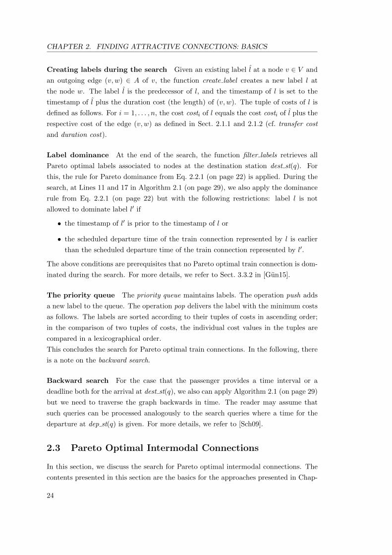
CHAPTER 2. FINDING ATTRACTIVE CONNECTIONS: BASICS
Creating labels during the search Given an existing label l at a node v ∈ V and
an outgoing edge (v, w) ∈ A of v, the function create label creates a new label l at
the node w. The label l is the predecessor of l, and the timestamp of l is set to the
timestamp of l plus the duration cost (the length) of (v, w). The tuple of costs of l is
defined as follows. For i = 1, . . . , n, the cost costi of l equals the cost costi of l plus the
respective cost of the edge (v, w) as defined in Sect. 2.1.1 and 2.1.2 (cf. transfer cost
and duration cost).
Label dominance At the end of the search, the function filter labels retrieves all
Pareto optimal labels associated to nodes at the destination station dest st(q). For
this, the rule for Pareto dominance from Eq. 2.2.1 (on page 22) is applied. During the
search, at Lines 11 and 17 in Algorithm 2.1 (on page 29), we also apply the dominance
rule from Eq. 2.2.1 (on page 22) but with the following restrictions: label l is not
allowed to dominate label l′ if
• the timestamp of l′ is prior to the timestamp of l or
• the scheduled departure time of the train connection represented by l is earlier
than the scheduled departure time of the train connection represented by l′.
The above conditions are prerequisites that no Pareto optimal train connection is dom-
inated during the search. For more details, we refer to Sect. 3.3.2 in [Gun15].
The priority queue The priority queue maintains labels. The operation push adds
a new label to the queue. The operation pop delivers the label with the minimum costs
as follows. The labels are sorted according to their tuples of costs in ascending order;
in the comparison of two tuples of costs, the individual cost values in the tuples are
compared in a lexicographical order.
This concludes the search for Pareto optimal train connections. In the following, there
is a note on the backward search.
Backward search For the case that the passenger provides a time interval or a
deadline both for the arrival at dest st(q), we also can apply Algorithm 2.1 (on page 29)
but we need to traverse the graph backwards in time. The reader may assume that
such queries can be processed analogously to the search queries where a time for the
departure at dep st(q) is given. For more details, we refer to [Sch09].
2.3 Pareto Optimal Intermodal Connections
In this section, we discuss the search for Pareto optimal intermodal connections. The
contents presented in this section are the basics for the approaches presented in Chap-
24

2.3. PARETO OPTIMAL INTERMODAL CONNECTIONS
ter 8. Pareto optimal intermodal connections and the search for them in time-dependent
graphs have been introduced by [Gun15, Gun14, Arn14, GKSW14]; an application and
extension can be found in [FGKS16]. The content presented in this section is taken
from those works.
From Sect. 1.4, recall that each intermodal connection consists of a train connection
and two parts where individual modes of transport are used. In intermodal connections,
the criteria which are relevant to passengers are usually travel time, price, and number
of transfers (convenience). Each criteria must be assessed by taking into account the
entire connection including the parts where individual modes of transport are used. The
search approach, as explained here, computes Pareto optimal intermodal connections
for each query such that the intermodal connections are optimized in their entirety.
Note: Alternatively, we could separately optimize the train connection and the parts
with individual modes of transport, and, subsequently, merge them to an intermodal
connection. However, such intermodal connections are not necessarily optimal—in their
entirety—according to the criteria relevant to passengers.
Queries A query q comprises
• a starting location where the passenger starts traveling,
• a destination location where the passenger ends traveling,
• either a time interval [begin(q), end(q)] or a point in time ontrip time(q) each for
the start time of the journey at the starting location, and
• a list of individual modes of transport which can be used.
A location could be provided for example as GPS coordinates or addresses. The values
ontrip time(q), begin(q), and end(q) are times in the set TIMES.
The search approach The search for Pareto optimal intermodal connections has
three steps. First, we retrieve all individual routes connecting the departure location
as well as the destination location with public transport. These are routes where pas-
sengers travel by individual modes of transport; they can be used as initial and end
parts of intermodal connections. In the second step, we add to the time-dependent
graph the individual routes that are computed for the end parts of intermodal connec-
tions. The result is a graph representing the timetable for public transport as well as
the individual routes for the end parts of intermodal connections. Finally, in the third
step, the set of all Pareto optimal connections is computed by applying the Pareto
Dijkstra algorithm on the resulting graph. In order to model the individual routes for
25

CHAPTER 2. FINDING ATTRACTIVE CONNECTIONS: BASICS
the initial parts of intermodal connections, we modify the procedure of creating start
labels (cf. Sect. 2.2.2, Creating start labels). In Sect. 2.3.1–2.3.3, we discuss each step
more precisely.
2.3.1 The First Step: Computing Individual Routes
First, we introduce individual routes. Each individual route describes how to travel by
a specific individual mode of transport either from the starting location to a public
transport station or from a public transport station to the destination location; it has
a duration (time cost) and a price. Such routes can be computed by routing engines
as presented in [LV11].
The first step of the search is illustrated in Fig. 2.3 (on page 27). Given a starting
location and a destination location, the first step computes and delivers all reasonable
individual routes to travel from the starting location to public transport stations (in
the near of the starting location) and from public transport stations (in the near of the
destination location) to the destination location. Whether a route is reasonable or not
depends on its duration. For each individual mode of transport, a specific maximum
duration is defined. Routes which have durations longer than this maximum value are
not reasonable. These maximum durations, also called ranges, are parameters which
can be specified by the passengers.
Station-based modes For car sharing and bike sharing, we focus on the station-
based model as illustrated in Fig. 1.4 (on page 12); such an individual route consists of
three parts as follows. For the initial part of intermodal connections, an individual route
begins at the starting location; the passenger walks to a car sharing or a bike sharing
station in order to collect the car or the bike respectively. He/she then drives to a car
sharing or a bike sharing station in the near of a public transport station, and returns
the car or the bike respectively. Last, the passenger walks to the public transport
station. For the end part of intermodal connections, the structure of individual routes
is analogous.
Modes without stations In contrast, individual routes for modes of transport such
as walks, taxis, individual bikes, and individual cars begin at the starting location and
end at a public transport station. For the end part of intermodal connections, the
structure of individual routes is analogous.
Note: We assume that passengers can park individual cars and bikes in the near of
public transport stations.
26

2.3. PARETO OPTIMAL INTERMODAL CONNECTIONS
public transport
Figure 2.3: The figure illustrates the structure of intermodal connections as well as, respectively, threedifferent ranges of three individual modes of transport around the starting location (left) and aroundthe destination location (right). The thin arrows illustrate the movements by individual modes oftransport from the starting location to public stations (left) and from public stations to the destinationlocation (right). By way of example, the inner, middle, and outer circle are the ranges for walk, bike,and car respectively. This figure has been taken from Figure 6.1 in [Gun15].
2.3.2 The Second Step: Extending the Graph
The next step is to extend the time-dependent graph (cf. Sect. 2.1.2) that models
the timetable by the individual routes computed for the end parts of the intermodal
connections. For this, the graph is extended for each search query, and this modification
is rolled back after the query is processed.
Modeling the end part First, we add to the graph a node that represents the
destination location of the connections; we denote it by the destination node. We then
model each individual route from a public transport station to the destination location
by an individual transport edge from the station node of that station to the destination
node. In contrast to route edges (cf. Sect. 2.1.2), the duration of an individual transport
edge is not time-dependent; it has a fixed travel time and a fixed price; these values
are taken from the respective individual route. The transfer cost equals zero.
Note: To model the start part of the intermodal connections, where individual modes
of transport are used, we modify the Pareto Dijkstra algorithm as will be explained in
Sect. 2.3.3.
2.3.3 The Third Step: Pareto Dijkstra
In the last step, the Pareto Dijkstra algorithm from Sect. 2.2 is applied to find all
Pareto optimal intermodal connections. In order to model the individual routes for
the initial parts of intermodal connections, the procedure of creating start labels (cf.
Sect. 2.2.2) is modified. Briefly, we create start labels for each individual route that is
computed in the first step of the search for the initial parts of intermodal connections
27

CHAPTER 2. FINDING ATTRACTIVE CONNECTIONS: BASICS
(cf. Sect. 2.3.1); a more precise explanation follows.
Modeling the initial part Each individual route computed for the initial parts of
intermodal connections is modeled as follows. Recall that such an individual route ends
at a public transport station s ∈ S, and it has a travel time (time cost) as well as a
price. In the on-trip scenario where, in the query q, a point in time ontrip time(q)
is given as the start time of the journey at the starting location, we merely create a
start label at the station node of the station s. The timestamp of this label is set to
ontrip time(q) plus the travel time of the individual route.
On the other hand, if a time interval [begin(q), end(q)] is given as the start time of
the journey, we create a new label for each departure event edep ∈ Esdep at s where
sched(edep)− δ ∈ [begin(q), end(q)];
the value δ is the travel time of the individual route. The new label is associated to the
route node that represents edep, and the timestamp of the new label is set to sched(edep).
In both cases, the time cost of the start label and its price (if price is a Pareto
criterion) are set to the respective values of the individual route. This concludes the
search for Pareto optimal intermodal connections. For more details, we refer to [Gun15].
2.4 Conclusion
In this chapter, we discussed the time-expanded and the time-dependent graph model;
both can be applied in order to model a timetable. The time-dependent model is more
efficient in modeling timetables including short-range local transit such as buses and
streetcars. For a timetable without short-range transit, the time-expanded model could
be applied as well; advantageously, it correctly models platform-specific interchange
times. We then explained the Pareto concept as a quality measurement for train and
intermodal connections. We also discussed the Pareto Dijkstra algorithm computing
Pareto optimal train and intermodal connections. In the rest of this work, we will use
the models and the methods presented in this chapter.
28

2.4. CONCLUSION
Data: timetable TT; query qResult: set of all Pareto optimal labels at the destination
1 DL← ∅; /* set of labels at the destination */
2 foreach v ∈ V do3 L(v)← ∅; /* initialize the set of labels at each node */
4 end/* Initialize the priority queue with the start labels */
5 pq ← create start labels();6 while pq is not empty do
7 l← pq.pop();
8 v ← the node of l;9 foreach (v, w) ∈ A do /* outgoing edges of v */
10 l← create label(l, (v, w));/* check whether l is dominated */
11 if @l′ ∈ L(w) : l′ dominates l then12 if w is at the destination then13 DL← DL ∪ {l};14 else15 pq ← pq ∪ {l};16 L(w)← L(w) ∪ {l};
/* Remove all labels dominated by l */
17 foreach l′ ∈ L(w) : l dominates l′ do18 L(w)← L(w) \ {l′};19 end
20 end
21 end
22 end
23 end24 filter labels(DL);
Algorithm 2.1: The Pareto Dijkstra algorithm. Labels and the priority queue aswell as the functions create label, create start labels, filter labels, pop, and pushare as defined in Sect. 2.2.2.
29


Chapter 3
Reliability Assessment
3.1 Introduction
Timetable information systems basically compute and deliver train connections that
optimize the criteria of travel time, number of transfers, and price. The train connec-
tions delivered are feasible according to the timetable that is valid at the computation
time. In other words, such a train connection allows a passenger to travel from his/her
start station to his/her destination station as long as the trains in the train connection
adhere to the timetable that is valid at the computation time. In a real-world train
network, unfortunately, train delays are common and disrupt the timetable. Moreover,
train cancelations and reroutings affect the daily operation of trains.
From Sect. 1.3 (cf. Feasible transfers), recall that the feasibility of a transfer activity
(es1,tr1dep , es2,tr2
arr ) ∈ TRANS depends on the real times of the events es1,tr1dep and es2,tr2
arr . If tr1
arrives too late, the transfer breaks; the train connection becomes infeasible according
to the real times. Delays which result in infeasible train connections are not infrequent.
Probability of success An important characteristic of each train connection is its
reliability regarding disruptions in the timetable. In our model, the reliability of a train
connection c is defined by the probability that, when taking c, passengers can travel to
their destination even if delays disrupt the timetable; meaning the probability that c
will be feasible according to real times (cf. Sect. 1.3, Feasible train connections). We
denote this probability as the probability of success.
The probability of the success of a train connection depends on the transfers in
the train connection. Train connections with transfers that tend to break have a lower
probability of success compared to train connections with transfers that retain a high
probability of feasibility. The definition of probability of success also applies to transfers;
it is the probability that the transfer will be feasible according to real times (cf. Sect. 1.3,
Feasible transfers).
31

CHAPTER 3. RELIABILITY ASSESSMENT
The method of assessing the reliability In this chapter, we present a method
of assessing the reliability of a train connection; the method computes the probability
of the success of the train connection. Our method is based on realistic, stochastic
predictions for the real times of the departure and arrival events in the timetable.
Each of these predictions is a probability distribution; more precisely, for each event
e ∈ E and for each time t ∈ TIMES, we compute the probability that e takes place
at the time t; that is, the real time of e equals t. These probability distributions are
computed by taking into account historical delay data, the current situation in the
railway network, and the interdependencies between the trains. The interdependencies
between the trains are caused by delay managements; trains wait for the passengers
of other delayed trains. Our computational study in Sect. 9.3 demonstrates that our
reliability assessments are realistic and accurate.
Note: As discussed in Sect. 3.2, the stochastic predictions have been introduced in
[BGMHO11].
Overview In Sect. 3.2, we discuss the state of the art and related methods for reli-
ability assessment. Our method of assessing the reliability is based on a model with
stochastic predictions for the real event times; the definition of the model can be found
in Sect. 3.3. In Sect. 3.4 and 3.5, we discuss the formulas employed to compute these
distributions. In Sect. 3.6 and 3.7, we present our method of computing the probability
of success for transfers and train connections. After that, in Sect. 3.8, we present ap-
proaches to precomputing the probability distributions of the events in the timetable
in order to accelerate the reliability assessment of train connections. We discuss, in
Sect. 3.9, how to update the probability distributions for the random event times ac-
cording to the real-time incidents introduced in Sect. 1.3.1. In Sect. 3.10, we analyze the
asymptotic complexity of our reliability assessment method. In Sect. 3.11, we discuss
an assumption of independence which is a prerequisite for our reliability assessment
method. In Sect. 3.12, we address how train cancelations and reroutings could be in-
corporated into the reliability assessment. Finally, in Sect. 3.13, we offer details on our
implementation of the reliability assessment method presented in this chapter. This
chapter is concluded in Sect. 3.14.
3.2 Related Work
The computation of the probability of the success of a train connection, considering
(I) the interdependencies between trains which could have effects on the feasibility
of the train connection as well as (II) the fact that train connections can consist of
multiple transfer activities, has not been addressed so far to the best of our knowledge.
32

3.2. RELATED WORK
The authors of [MHS09] presented an efficient model to propagate deterministic delays
through train networks; a computation of the probability of success is not supported by
their model. Stochastic delay propagations and predictions of train delays have been
investigated in various works; examples are the works presented by [MM07, BGMHO11,
CK94, MDnP10].
A method of assessing the reliability of a train connection is evaluating the buffer
times of the train connection’s transfer activities; this method is addressed in [Meh07,
Sch09]. The buffer time of a transfer activity (es1,tr1arr , es2,tr2
dep ) ∈ TRANS is the time
difference (sched(es2,tr2
dep )− sched(es1,tr1arr )
)−min dur(es1,tr1
arr , es2,tr2dep ).
Unfortunately, a mere analysis of the buffer times could result in inaccurate assessments.
While a specific buffer time could be even more than necessary for a transfer activity
to be reliable, it could be insufficient for another one.
Lemnian et al. proposed a method of computing the probability of the success of
a transfer activity [LRR+14]. Their model relies on probability distributions for the
durations of the train moves (as will be discussed in Sect. 3.3) but does not take into
account the interdependencies between the trains which could affect the probability of
the success of the train connection; waiting time rules (cf. Sect. 1.3) are only taken into
account for the trains which are directly involved in the transfer activity but not for the
other departure events in the train connection. Moreover, for the reliability assessment,
each transfer in a train connection is evaluated in isolation. In contrast, our method
considers the dependencies between the transfer activities in each train connection.
The general idea of modeling the real event times by random variables has already
been introduced in [BGMHO11]; the stochastic model from Sect. 3.3 as well as the
interdependencies and the formulas discussed in Sect. 3.5.1 and 3.5.2 rely on the work
published by [BGMHO11]. However, in our opinion, the terminology and the formulas
presented here are easier to read and to understand. Moreover, we designed our model
such that we do not require an assumption made by them. In contrast to their model,
the real event time of the arrival events can be earlier than their scheduled event time.
Publication of the author In [KSWZ12], we have already presented the formula
for the computation of the probability of the success of a transfer activity. We used
there a terminology and a formula different than presented here. But both formulas
are equivalent as will be proved in Appx. A.1.
33

CHAPTER 3. RELIABILITY ASSESSMENT
3.3 Stochastic Model
In this section, we introduce our stochastic model that allows us to compute stochastic
predictions for the real times of the departure and arrival events in the timetable. As
explained in Sect. 3.1 (cf. The method of assessing the reliability), these stochastic
predictions are probability distributions for the events. Our method of assessing the
reliability of a train connection is based on these probability distributions. In addition,
in Chapters 4–8, we will discuss approaches of computing reliable train connections
and journeys; these approaches are based on the stochastic model from this section.
First, we begin with an informal description of our stochastic model; we then present
the formal definition.
3.3.1 Informal Description
From Sect. 1.1 and 1.3.2, recall that each departure and arrival event has a scheduled
and a real event time. While the scheduled time may be looked up in the timetable,
the real event time depends on unforeseen circumstances, and it is not safely known
until the event takes place. Among the reasons are waitings of trains for each other
(due to delay management policies from cf. Sect. 1.3, Maximum waiting times), signal
disturbances, technical malfunctions, human resource problems, emergencies, weather
conditions, etcetera. These factors influence the real event time of each departure and
arrival event.
Random event times In our model, for each event, there is a random variable mod-
eling its unknown real time; this random variable is called the random event time of the
event. The delay origins (see above) are modeled by defining stochastic dependencies of
random event times. We distinguish between delays arisen from the interdependencies
between the events in the timetable and delays from other origins such as technical
malfunctions, signal disturbances, etc. The interdependencies between the events are
modeled by defining interdependencies between the random times of the events. Thus,
the random event time of each event stochastically depends on the random event times
of a specific set of events in the timetable as will be detailed in Sect. 3.5.1. To incorpo-
rate the other delay origins into our model, we introduce a random prepared time for
each departure event as well as a random duration for each train move.
Note: The interdependencies between the events are detailed in Sect. 3.5.1. In short,
they are caused by the waiting times of the trains as defined in Sect. 1.3.2 (cf. Maximum
waiting times). In addition, each event of each train stochastically depends on the
preceding events of that train; for example, a train cannot depart from a station before
34

3.3. STOCHASTIC MODEL
it arrives at that station.
Random prepared times For each departure event etr,sdep ∈ Edep, the prepared time
denotes the time when the train tr is ready to depart from s. According to the timetable,
this time equals sched(etr,sdep). In contrast, the real prepared time is unknown and can be
later than sched(etr,sdep) because of a delayed train delivery (only for the very first depar-
ture events), technical malfunctions, human resource problems, emergencies, weather
conditions, etcetera. Hence, for each departure event, we introduce a random variable
modeling the unknown, real prepared time of the departure event; it is denoted as the
random prepared time. The random event time of a departure event consequently has
a stochastic dependency on its random prepared time.
Random train move durations We furthermore introduce, for each train move, a
random variable denoted as the random train move duration; it models deviations from
the scheduled duration of the train move. Delays during a train move could result in a
delayed arrival. On the other hand, it is possible that the duration of the train move is
shorter than scheduled. The most of the problems resulting in delayed prepared times
could occur during a train move as well. In addition, trains could be instructed to wait
for a track to be freed.
The real duration of a train move depends on the real event time of its departure
event. This dependency may have positive and negative effects and, hence, covers both
fundamental cases: the delayed departure edep causes further delays during the move,
or the train operator decides to “step on the gas” along (edep, earr) in order to make up
for the delayed departure edep.
A formal description of the random variables introduced above can be found in
Sect. 3.3.2.
3.3.2 Formal Description
Each random variables in our model is discrete; it has a discrete probability distri-
bution with a discrete probability density function f : TIMES 7→ [0, 1] ⊂ R where∑t∈TIMES f(t) = 1. For a random variable X with the probability density function fX ,
the probability that X assumes the value t equals P (X = t) = fX(t). The support of
fX comprises each time t ∈ TIMES where fX(t) > 0; it is denoted by supp(fX).
Random event times For each event e ∈ E, the discrete random variableXe denotes
the random event time of e. There is a joint probability distribution with the dimension
|E| over all random variables Xe, e ∈ E. For each event e ∈ E, the probability density
35

CHAPTER 3. RELIABILITY ASSESSMENT
function of the marginal distribution of Xe is denoted by φ(e). The value φ(e, t) equals
P (Xe = t); the probability of the event e taking place at the time t.
In our model, we assume that trains never depart earlier than scheduled. In contrast,
arrivals earlier than scheduled are possible.
Random prepared times For each departure event edep ∈ Edep, the random vari-
able Xpedep denotes the random time when the train is prepared for the departure. There
is a joint probability distribution over all random variables Xpedep , edep ∈ Edep with the
dimension |Edep|. For each departure event edep ∈ Edep, the probability density func-
tion of the marginal distribution of Xpedep is denoted by ξ(edep). The value ξ(edep, t)
equals P (Xpedep = t); the probability that the real prepared time of edep equals t.
Random durations of train moves The discrete random variable Xtm denotes
the random duration of the train move tm = (edep, earr) ∈ TM. For each time tdep ∈TIMES, there is a joint probability distribution Θ(TM, tdep) with the dimension |TM|over all random variables Xtm, tm ∈ TM. For each tm ∈ TM and each tdep ∈ TIMES,
the probability density function of the marginal distribution of Xtm is denoted by
θ(tm, tdep). The parameter tdep models the dependency of the random duration of the
train move (edep, earr) on the real departure time of edep. For the times tdep, tarr ∈TIMES and tm = (edep, earr) ∈ TM, we define
θ(tm, tdep, tarr) = P (Xtm = tarr − tdep | Xedep = tdep)
= P (Xearr = tarr | Xedep = tdep);
in words, the value θ(tm, tdep, tarr) is the conditional probability that the real duration
of tm equals tarr− tdep given that the departure event edep takes place at the time tdep.
This concludes our stochastic model. In Sect. 3.4, we focus on the computation of
the marginal distributions for random prepared times and random train moves dura-
tions. The interdependencies between the random times of the events as well as the
computation of their probability distributions are discussed in Sect. 3.5.
3.4 Distributions for Prepared Times and Train Move Du-
rations
The computation of probability distributions for random train move durations and
random prepared times (cf. Sect. 3.3) is not on the focus of this work. In our com-
putational study in Chapter 9, for these random variables, we mainly use probability
distributions provided to us by the German railway company. However, to make this
36

3.4. DISTRIBUTIONS FOR PREPARED TIMES AND TRAIN MOVEDURATIONS
work self-contained, in this section, there is an excursion into the computation of prob-
ability distributions for these random variables. A reader, who is not interested in this
step, may skip this section and continue with Sect. 3.5.
The random variables for random prepared times and random durations of train
moves model a broad range of delay reasons. The more realistic their probability
distributions are, the more accurate are computations basing on them. We discuss
two general ideas to obtain these probability distributions: either to learn them from
historical data or to generate realistic ones. While the former is more accurate and
convincing, the latter could be a solution if no historical data is available.
Note: In the bachelor’s theses by Julian Gross [Gro15] and Marco Plaue [Pla16], we
evaluated approaches to the learning of probability distributions.
3.4.1 Prepared Times: Learn from Historical Data
For a timetable TTfut with a validity period in the future, the probability distributions
for the random prepared times of the departure events (cf. Sect. 3.3) can be learned
from historical data. More precisely, we learn from a given timetable TThist with a
validity period TIMEShist in the past where the real time real(e) of (almost) each event
e ∈ Ehist is already known. Events in the set Ehist in TThist with unknown real times
(unknown because of lack of data) are excluded from the learning procedure.
We learn probability distributions for random prepared times in two successive
steps. In the first step, we divide all departure events in Edep into disjunct subsets;
this step is performed equally for TThist and TTfut. Each of these subsets is denoted
as a class. Thus, for each of TThist and TTfut, we obtain a set of classes; these two sets
are denoted by EChistdep ⊂ 2E
histdep and ECfut
dep ⊂ 2Efutdep respectively. This classification has
the following background. The random prepared times of all departure events in the
same class can be described by the same probability distribution since these departure
events are equivalent according to specific properties as will be explained below (cf.
First step: classification). The classification is performed by a classification function
c : Edep 7→ 2Edep equally for TThist and for TTfut. Thus, for each class in EChistdep , there
is a respective class in ECfutdep and vice versa.
In the second step of the learning procedure, for each class in ECfutdep, a probability
distribution is learned by evaluating the real prepared times of the departure events in
the respective class in EChistdep . The result is a probability distribution that is valid for
the random prepared times of each departure event in that class. In other words, this
probability distribution describes the random prepared time of each departure event in
the respective class in ECfutdep.
The two steps of the learning procedure are detailed in the following.
37

CHAPTER 3. RELIABILITY ASSESSMENT
First step: classification For the classification of the departure events, we define
the classification function c : Edep 7→ 2Edep . A set of properties of the departure events
is specified; the classification function is designed such that all departure event sharing
the same properties—from the set of properties specified—are assigned to the same
class. The set of the properties selected for the classification should be defined depend-
ing on the characteristics of the timetable and the railway network. First, the train
category (such as intercity express, regional train, streetcar, etc.) usually influences
the frequency and the extent of delayed prepared times. For example, for different
train categories, different types of vehicles are used. Two further properties potentially
influencing the prepared time of each event are the scheduled departure time of the
event (e.g. morning, noon, after noon, evening) and the size of the station where the
event takes place.
Note: The validity period of TThist should be as long as it contains sufficient samples
for each class. Theoretically, the more crucial properties of the departure events are
selected for the classification, the more accurate is the results will be. In practice, for
a fine granular view on the data, we are faced by small numbers of samples. The
significance and expressiveness of the results consequently suffer from a fine granular
view on the data. Therefore, a suitable set of parameters needs to be chosen depending
on the timetable TThist and portion of events in Ehist for which data about the real
event times are actually available in TThist.
Note: Historical data contain outliers and potential errors which must be reasonably
managed.
Second step: computation Once the departure events in TThist are classified, for
each class in EChistdep , we compute a histogram of the differences between the real and
the scheduled event times over all departure events in that class. Then, a probability
density function for that class is obtained by normalizing the histogram to 1. These
probability density function describes the random prepared time of each departure
event in the respective class in TTfut (see below).
Assignment to ξ(edep, tdep) Once probability density functions are computed as
discussed above, they are assigned to the probabilities ξ(edep, tdep) (cf. Sect. 3.3.2,
Random prepared times) which describe the random prepared time of each depar-
ture event edep ∈ Efutdep of the timetable TTfut. More precisely, for each departure
event edep ∈ Efutdep, we apply the classification function in order to find the respective
class in EChistdep . Then, for each time tdep ∈ TIMESfut, the probability for the value
tdep − sched(edep) is retrieved—from the probability density function of that class—
38

3.4. DISTRIBUTIONS FOR PREPARED TIMES AND TRAIN MOVEDURATIONS
and assigned to ξ(edep, tdep) (recall that the probability density function comprise a
probability for each deviation from the scheduled event time).
Interdependencies between the events From Sect. 3.3.1, recall that each depar-
ture delay could either be caused by the interdependencies between the trains in the
timetable or have another origin like technical malfunctions, human resource prob-
lems, etc. By random prepared times, we model the latter. Some of the delays in
the timetable TThist could be caused by interdependencies between the events; conse-
quently, they have delay origins which we do not model by random prepared times. For
correct results, these delays should be excluded from the learning procedure and the
computation of the probabilities.
3.4.2 Train Move Durations: Learn from Historical Data
For a timetable TTfut with a validity period in the future, the probability distributions
for the random train move durations (cf. Sect. 3.3.2) can be learned from historical
data. More precisely, we learn from a given timetable TThist with a validity period
TIMEShist in the past where the real time real(e) of (almost) each event e ∈ Ehist is
already known. Events in the set Ehist in TThist with unknown real times (unknown
because of lack of data) are excluded from the learning procedure.
The learning procedure is similar as for random prepared times (cf. Sect. 3.4.1); it
has two successive steps. In the first step, we divide all train moves in TM into disjunct
subsets; this step is performed equally for TThist and TTfut. Each of these subsets is
denoted as a class. Thus, for each of TThist and TTfut, we obtain a set of classes; these
two sets are denoted by TMChist ⊂ 2TMhist and TMCfut ⊂ 2TMfut respectively. This
classification has the following background. The random durations of all train moves in
the same class can be described by the same probability distribution since these train
moves are equivalent according to specific properties as will be explained below (cf.
First step: classification). The classification is performed by a classification function
c : TM 7→ 2TM, equally for TThist and for TTfut. Thus, for each class in TMChist, there
is a respective class in TMCfut and vice versa.
In the second step of the learning procedure, for each class in TMCfut, a probabil-
ity distribution is learned by evaluating the real durations of the train moves in the
respective class in TMChist. The result is a probability distribution that is valid for
the random train move durations for each train move in that class. In other words,
this probability distribution describes the random duration of each train move in the
respective class in TMCfut.
The two steps of the learning procedure are detailed in the following.
39

CHAPTER 3. RELIABILITY ASSESSMENT
First step: classification For the classification of the train moves, we define the
classification function c : TM 7→ 2TM. A set of properties of the train moves is speci-
fied; the classification function is designed such that all train moves sharing the same
properties—from the set of properties specified—are assigned to the same class. The
set of the properties selected for the classification should be defined depending on the
characteristics of the timetable and the railway network. For the classification of the
train moves, the following properties could be taken into account:
• Departure delay : For a train move tm = (edep, earr), the delayed departure—i.e.
the difference between the real and the scheduled event time of edep—influences
the real duration of tm. A delayed departure could cause further delays during
the move, or the train operator could decide to “step on the gas” along (edep, earr)
in order to make up for the delayed departure edep.
• Train categories: The train category usually influences the delays. For example,
for different train categories, different types of vehicles are used; as a consequence,
they have different capabilities to make up for delays.
• Scheduled duration: Short and long rides could be affected from delays to dif-
ferent extents. Train moves over longer distances (resulting in longer scheduled
durations) could be more likely to be affected by delays that are caused during
train moves. On the other side, over a longer distance, the chance to make up
for delays is greater. To model these influences, the scheduled durations of train
moves should be incorporated into the definition of the classification function c.
• As further parameters, we could take into account the departure and arrival
stations of the train moves, information about the infrastructure of the railway
network (e.g. tracks), temporal attributes, etc.
For each train move tm = (edep, earr) in the timetable TTfut, all properties listed above
can be retrieved from TTfut except for the real time of edep since it is unknown. Con-
sequently, we cannot classify the train moves in TTfut by a classification function that
requires the departure delay as a parameter. To overcome this problem, we use a two
steps classification. First, we build the classes TMChist and TMCfut by employing a
classification function that incorporates all properties specified except for the depar-
ture delay. We then perform a second classification; we divide all train moves in each
class from the set TMChist into a set of subclasses such that the departure events of all
train moves in the same subclass have the same departure delay. Then, we proceed as
follows.
40

3.4. DISTRIBUTIONS FOR PREPARED TIMES AND TRAIN MOVEDURATIONS
Second step: computation Once the train moves in TThist are classified into
TMChist and subsequently into subclasses according to the departure delays (see above),
for each subclass, we compute a histogram of the differences between the real and the
scheduled durations over all train moves in that subclass. Then, a probability den-
sity function for that subclass is obtained by normalizing the histogram to 1. These
probability density function describes the random duration of each train move in the
respective class in TTfut (see below).
As discussed above, for TTfut, the departure delay is unknown. Therefore, the
real departure time tdep of the event edep of each train move (edep, earr) is an additional
parameter for the value θ(tm, tdep, tarr); for each departure delay expected, a probability
density function is computed.
Assignment to θ(tm, tdep, tarr) Once probability density functions are computed as
discussed above, they are assigned to the probabilities θ(tm, tdep, tarr) (cf. Sect. 3.3.2,
Random durations of train moves) which describe the random duration of each train
move tm ∈ TMfut of the timetable TTfut. More precisely, for each train move
(edep, earr) ∈ TMfut and two times tdep, tarr ∈ TIMESfut, we apply the classification
function c for (edep, earr) and find the respective class in TMChist. Finally, from the
probability density function of the subclass for the departure delay tdep − sched(edep),
the probability for the value
(tarr − tdep)− (sched(earr)− sched(edep))
is delivered and assigned to θ(tm, tdep, tarr).
Note: In our computational study in Chapter 9, for the random train move durations,
we use probability distributions provided to us by the German railways. These probability
distributions are classified by the real departure time, train category, and scheduled train
move duration.
Note: The validity period of TThist should be as long as it contains sufficient samples
for each class. Historical data contain outliers and potential errors which must be
reasonably managed.
3.4.3 Generate Distributions
Learning probability distributions requires historical data. For the case that historical
delay data is not available, realistic probability distributions for prepared times and
train move durations could be generated. In our computational study in Sect. 9.4, for
a subset of all train moves, we use probability distributions provided to us by Deutsche
41

CHAPTER 3. RELIABILITY ASSESSMENT
Bahn AG. For the rest of the train moves, we generate realistic probability distributions
using the Cauchy distribution [NIS17a]. The probability density function of a Cauchy
distribution is characterized by a location parameter and a scale parameter. The former
defines the position of the function’s peak on the x-axis; the latter stretches out the
graph [NIS17a]. To generate a probability density function describing the random
duration of a train move, we define the location and the scale parameter depending
on the scheduled duration of the train move and the delay of its departure event. The
scale parameter is defined such that we obtain wider distributions for train moves with
longer durations. The location parameter is defined such that in case of a delayed
departure the probability that the real duration is shorter than the scheduled duration
increases; we assume that the train makes up for the delayed departure. In Appx. A.3,
we present some examples.
3.5 Distributions for Random Event Times
In Sect. 3.3.2, we introduced random event times; for each event e ∈ E, there is a
probability density function φ(e) describing the random event time of e. Given a
timetable and the probability density functions for prepared times as well as train move
durations (as introduced in Sect. 1.1 and 3.3.2), for each e ∈ E, the probability density
function φ(e) can be determined. In Sect. 3.5.1, we explain the interdependencies
between the events and their random event times. We then discuss, in Sect. 3.5.2,
the formulas to compute the probabilities φ(e, t) for each event e ∈ E and each time
t ∈ TIMES. Our reliability assessment methods for transfers and train connections (cf.
Sect. 3.6 and 3.7) are based on those formulas.
3.5.1 The Interdependencies Between the Events
Fig. 3.1 (on page 43) demonstrates an illustrative example of dependencies between
departure and arrival events. In the following, we precisely explain these interdepen-
dencies.
3.5.1.1 The Dependencies of Departure Events
After the arrival of a train at a station and prior to its subsequent departure, the
minimum dwell time has to be obeyed according to the definition of dwell times from
Sect. 1.1 (cf. Dwell activities and times). In addition, a train does not depart until it
is prepared for the departure as introduced in Sect. 3.3 (cf. Random prepared times).
Furthermore, each train potentially waits for other delayed trains as introduced in
Sect. 1.3 (cf. Maximum waiting times).
42

3.5. DISTRIBUTIONS FOR RANDOM EVENT TIMES
es,tr2arr
es,trarr
es,tr3arr
es,trdep es2,tr
arr
transfer, max wait > 0dwell
transfer, max wait = 0
train move
Figure 3.1: The figure illustrates a section of a train network. The departure event es,trdep potentially
waits for the arrival event es,tr2arr but not for the arrival event es,tr3arr . Thus, it depends on the arrivalevents es,trarr and es,tr2arr . The arrival event es2,trarr only depends on es,trdep.
Set Edependarr (es,trdep) Hence, the random event time of each departure event es,tr
dep ∈ Edep
stochastically depends on a set of arrival events; we denote this set by Edependarr (es,tr
dep).
It comprises the following arrival events. First, if es,trdep is not the very first de-
parture event of the train tr, the arrival event es,trarr exists and is a member of the
set Edependarr (es,tr
dep). Second, the set Edependarr (es,tr
dep) comprises each arrival event es,tr2arr ∈ Es
arr
where max wait(es,tr2arr , e
s,trdep) > 0 (cf. Sect. 1.3, Maximum waiting times). Last, in order
to take into account the random prepared time of es,trdep, we add to the set Edepend
arr (es,trdep)
an artificial event es,trartific. For es,tr
artific, we introduce an artificial dwell activity dw =
(es,trartific, e
s,trdep) where min dur(dw) = 0. Moreover, we define φ(es,tr
artific, t) = ξ(es,trdep, t) for
t ∈ TIMES.
Consequently, the probability density function φ(edep) of a departure event edep ∈ Edep
is fully determined by the probability density functions of the arrival events in the set
Edependarr (edep).
3.5.1.2 The Dependencies of Arrival Events
The random time of each arrival event es,trarr ∈ Earr stochastically depends on the random
time of the departure event es2,trdep of the train move tm = (es2,tr
dep , es,trarr). The probability
density function φ(es,trarr) is fully determined by the probability density function φ(es2,tr
dep )
and the probability distribution of the random duration of the train move tm (cf.
Sect. 3.3.2).
Note: Our network is similar to a Bayesian network [Dar09] in the following sense.
We have a directed acyclic graph, where random variables Xe, e ∈ E, build the nodes
of the network. Each arrival event earr of a train move (edep, earr) has one predecessor,
the event edep. Set Edependarr (edep) comprises the predecessors of each departure event
edep. There is an arc from each predecessor of a node to the node itself. Each random
variable depends on its predecessors. However, in contrast to Bayesian networks, we do
43

CHAPTER 3. RELIABILITY ASSESSMENT
not explicitly create a conditional probability table for the random variables. Instead,
for each random variable Xe, we have a one-dimensional probability distribution.
3.5.2 The Calculation of the Probabilities
In this section, we introduce the formulas to compute the probabilities φ(e, t) for each
event e ∈ E and each time t ∈ TIMES.
3.5.2.1 The Formula for Departure Events
According to Sect. 3.5.1, the dependency of es,trdep on some arrival event es,tr2
arr ∈Edepend
arr (es,trdep) is based either on the minimum transfer time (in case tr 6= tr2) or on
the minimum dwell time (in case tr = tr2). Both of these times are described by
min dur(es,tr2arr , e
s,trdep) as defined in Sect. 1.1 and 1.2. Additionally, we define the latest
real event time of es,trdep that can be caused by es,tr2
arr ∈ Edependarr (es,tr
dep) as follows:
tlatestdep (es,tr2
arr , es,trdep) =
sched(es,trdep) + max wait(es,tr2
arr , es,trdep) if tr 6= tr2,
+∞ otherwise.(3.5.1)
The latter case models the trivial fact that each train waits for its own arrival without
any limit.
Informal description The stochastic event that a departure event edep ∈ Edep
takes place at the time tdep ∈ TIMES may be described as follows. First of all,
edep may take place at tdep only if edep does not have to wait for any arrival event
earr ∈ Edependarr (edep) up to some time t′dep > tdep according to the value tlatest
dep (earr, edep).
For tdep = sched(edep), this necessary condition is also sufficient since we assume that
a train never departs earlier than its scheduled departure time. On the other hand, for
tdep > sched(edep), an additional condition must be fulfilled: edep has to wait exactly
up to tdep for at least one earr ∈ Edependarr (edep). These informal descriptions may be
formalized as follows.
The formulas For each departure event edep ∈ Edep and each time tdep ∈ TIMES
where tdep ≥ sched(edep), let ψ(edep, tdep) denote the probability that the necessary
condition (see above) is fulfilled. More precisely, ψ(edep, tdep) is the probability that
edep does not have to wait for any arrival event in Edependarr (edep) up to some time
44
3.5. DISTRIBUTIONS FOR RANDOM EVENT TIMES
t′dep > tdep. For the time tdep ≥ sched(edep), we obtain:
ψ(edep, tdep) =∏
earr∈Edependarr (edep)
[P(Xearr + min dur(earr, edep) ≤ tdep
)+ P
(Xearr + min dur(earr, edep) >
max{tdep, tlatestdep (earr, edep)}
) ].
(3.5.2)
For tdep < sched(edep), we define ψ(edep, tdep) = 0 since we assume that a train never
departs earlier than its scheduled departure time. Hence, for a time tdep ≥ sched(edep),
we obtain
φ(edep, tdep) = P (Xedep = tdep) = ψ(edep, tdep)− ψ(edep, tdep − 1). (3.5.3)
The smallest value for tdep ∈ supp(φ(edep)) is sched(edep). Let tmax
(supp(φ(e))
)denote
the largest time in supp(φ(e)) for each event e ∈ E. More precisely, we define
tmax
(supp(φ(e))
)= max{sched(edep), max
earr∈Edependarr (edep)
tmaxdep (edep, earr)}
where the value tmaxdep (edep, earr) denotes the latest delayed departure time of edep that
may be caused by earr when taking into account the function φ(earr); it equals
tmaxdep (edep, earr) = min
{ cf. Eq. 3.5.1 (on page 44)︷ ︸︸ ︷tlatestdep (earr, edep) ,
tmax
(supp(φ(earr))
)+ min dur(earr, edep)
}.
Assumption of independence The formula to compute ψ(edep, tdep) is based on the
assumption that all random variables Xearr are stochastically independent for edep ∈Edep and each earr ∈ Edepend
arr (edep). This assumption is discussed in Sect. 3.11.
3.5.2.2 The Formula for Arrival Events
For each arrival event earr ∈ Earr of the train move tm = (edep, earr) and for each time
tarr ∈ TIMES, the probability φ(earr, tarr) is given by the convolution of φ(edep) with
the probability density functions for the real durations of tm:
φ(earr, tarr) = P(Xearr = tarr
)=
tarr∑tdep=sched(edep)
φ(edep, tdep) · θ(tm, tdep, tarr).(3.5.4)
45

CHAPTER 3. RELIABILITY ASSESSMENT
From Sect. 3.3.2, recall that θ(tm, tdep, tarr) is the probability that the train move tm
arrives at the time tarr given that the departure is at the time tdep. The range of the
values in supp(φ(earr)) is defined by the smallest and largest values for tarr such that
φ(edep, tdep) · θ(tm, tdep, tarr) > 0 for some time tdep. Recall that values earlier than
sched(earr) can be in supp(φ(earr)).
Bayes’ theorem Our formula to compute the probabilities φ(earr) is based on Bayes’
theorem. More precisely, we apply the law of total probability [NIS17b]; for stochastic
events A and B1, B2, . . . , Bn, n ∈ N, one has
P (A) =∑n
P (A | Bn) · P (Bn).
3.6 The Reliability Assessment of Transfers
In this section, we demonstrate our method of assessing the reliability of a transfer;
that is, the computation of the probability of the success of the transfer activity.
The Probability of the Success of a Transfer For a given transfer activity
(es1,tr1arr , es2,tr2
dep ) ∈ TRANS, the probability of success is the probability that the transfer
from tr1—arriving at s1—into tr2—departing from s2—is feasible according to the real
times of es1,tr1arr and es2,tr2
dep , as defined in Sect. 1.2 (cf. Feasible Transfers). Formally, it
is the following probability:
P(Xes1,tr1arr
+ min dur(es1,tr1arr , es2,tr2
dep ) ≤ Xes2,tr2dep
).
Note: From Sect. 1.2, recall that s1 6= s2 if (es1,tr1arr , es2,tr2
dep ) is a transfer activity with a
walk trip.
The calculation The probability of the success of a transfer activity (earr, edep) ∈TRANS equals
P(Xearr + min dur(earr, edep) ≤ Xedep
)=
∑tdep∈supp(φ(edep))
P(Xearr + min dur(earr, edep) ≤ tdep
∩ Xedep = tdep
).
(3.6.1)
46
3.6. THE RELIABILITY ASSESSMENT OF TRANSFERS
The value P (Xearr + min dur(earr, edep) ≤ tdep ∩ Xedep = tdep) in Eq. 3.6.1 is the
probability that the transfer is feasible if edep takes place at the time tdep; in other
words, the joint probability that earr takes place no later than tdep−min dur(earr, edep)
and edep takes place at the time tdep (recall that Xedep potentially depends on Xearr).
This probability is defined as follows:
P(Xearr+ min dur(earr, edep) ≤ tdep ∩ Xedep = tdep
)=
ϑ1 if tdep ≤ sched(edep) + max wait(earr, edep),
ϑ2 otherwise
(3.6.2)
where
ϑ1 = P (Xearr + min dur(earr, edep) ≤ tdep) · ψearr(edep, tdep)
− P (Xearr + min dur(earr, edep) ≤ tdep − 1) · ψearr(edep, tdep − 1)
and
ϑ2 = P (Xearr + min dur(earr, edep) ≤ tdep)
·[ψearr(edep, tdep)− ψearr(edep, tdep − 1)
].
The probability ψearr(edep, tdep) is computed with the formula defined for ψ(edep, tdep)
in Eq. 3.5.2 (on page 45) but with one difference: the product in Eq. 3.5.2 is computed
over all arrival events in the set Edependarr (edep) \ {earr} instead of the set Edepend
arr (edep).
Assumption of independence In Sect. 3.5.2.1 (cf. Assumption of independence),
we already introduced our assumption of independence for the computation of the
functions φ(e), e ∈ E. Analogously, to compute P(Xearr + min dur(earr, edep) ≤ Xedep
),
we assume that the random event times of the arrival event earr and the arrival events
in the set Edependarr (edep) \ {earr} are stochastically independent. This assumption will
be discussed in Sect. 3.11.
Explanations Obviously, Eq. 3.6.2 (on page 47) is a modification of the formula
from Eq. 3.5.3 (on page 45) employed to compute φ(edep) for a departure event edep.
By introducing ψearr(edep, tdep), the arrival event earr is omitted from the computation
of the product in Eq. 3.5.2 (on page 45). Instead, the arrival event earr is incorporated
into the formula individually. The reason is that, according to Eq. 3.6.1 (on page 46),
we need to compute the probability for the case that the transfer activity (earr, edep) is
feasible; for real event times of earr later than tdep −min dur(earr, edep), the transfer is
infeasible.
Moreover, a distinction is required between the cases where edep waits for earr
47

CHAPTER 3. RELIABILITY ASSESSMENT
es,trarr
es,tr2arr
es,tr3arr
es,tr2dep es2,tr2
arr
transfer
dwell
transfe
r
move
Figure 3.2: The figure illustrates a section of a train network. The reliability of the transfer activity(es,trarr , e
s,tr2dep ) ∈ TRANS should be assessed. There is a dwell activity (es,tr2arr , e
s,tr2dep ) ∈ DW. The departure
event es,tr2dep potentially waits for es,trarr and es,tr3arr . The chart bars above the events represent the probability
density functions φ(e) for each event e. In addition, for es,tr2dep and each tdep ∈ supp(φ(es,tr2dep )), the
probability P(X
es,trarr
+ min dur(es,trarr , es,tr2dep ) ≤ tdep ∩ X
es,tr2dep
= tdep)
is illustrated as a dashed part of
the respective bar.
or where not. For tdep ≤ sched(edep) + max wait(earr, edep), a delayed arrival time
of earr influences the real event time of edep. In contrast, for tdep > sched(edep) +
max wait(earr, edep), the departure of edep at tdep is independent from the arrival time
of earr.
If edep does not wait for earr at all, Xedep does not depend on Xearr . In that case,
the probability from Eq. 3.6.2 (on page 47) equals
P (Xearr + min dur(earr, edep) ≤ tdep) · φ(edep, tdep).
This also applies if (earr, edep) is a transfer activity with a walk.
Note: For each transfer activity (earr, edep) ∈ TRANS and each time tdep ∈ TIMES,
observe that
P(Xearr + min dur(earr, edep) ≤ tdep ∩Xedep = tdep
)≤ φ(edep, tdep).
An illustrative example Fig. 3.2 demonstrates an illustrative example of the de-
pendencies between departure and arrival events which play a role when computing
the probability of the success of a transfer. In the example, the real event time of the
48
3.7. THE RELIABILITY ASSESSMENT OF TRAIN CONNECTIONS
departure event es,tr2dep depends on the arrival events es,tr
arr , es,tr2arr , and es,tr3
arr . Thus, the set
Edependarr (es,tr2
dep ) (as introduced in Sect. 3.5.1) comprises these three arrival events. The
support of φ(e) for each event e in the example is limited to zero till three minutes
delay. We assume that a passenger arrives with the train tr at the station s and plans
to transfer into the train tr2. To assess the probability of the success of the trans-
fer activity (es,trarr , e
s,tr2dep ) ∈ TRANS, the formula presented in Eq. 3.6.1 (on page 46) is
applied.
3.7 The Reliability Assessment of Train Connections
In this section, we introduce the reliability assessment of train connections. To assess
the reliability of a train connection, we compute its probability of success.
The Probability of the Success of a Train Connection This is the probability
that the train connection will be feasible according to the real times (cf. Sect. 1.3.2).
In other words, it is the probability that the train connection does not break because
of delays.
As defined in Sect. 1.2, a train connection is a sequence of train and walk trips;
there is a transfer activity between each pair of train trips which appear in the train
connection successively. For a train connection c with k ∈ N0 transfers, let (ejarr, ejdep) ∈
TRANS, j = 1, . . . , k, denote the transfer activities in c. Formally, the probability of
the success of the train connection c equals
P( ⋂j=1,...,k
Xejarr
+ min dur(ejarr, ejdep) ≤ X
ejdep
). (3.7.1)
In the following, we discuss how the above probability is calculated.
3.7.1 The Calculation
To compute the probability from Eq. 3.7.1 for a train connection c, first, we introduce
a stochastic event.
The stochastic event Fi Let e1, e2, . . . , en denote the sequence of all departure and
arrival events in the train connection c where n ∈ N>0 is the number of all events in c.
For i ∈ 1, 2, . . . , n, we introduce Fi; it denotes the stochastic event that the part of c
from e1 to ei is feasible according to real times (cf. Sect. 1.3.2) if the events e1, e2, . . . , ei
take place. According to Eq. 3.7.1, we obtain
P( ⋂j=1,...,k
Xejarr
+ min dur(ejarr, ejdep) ≤ X
ejdep
)= P (Fn)
49

CHAPTER 3. RELIABILITY ASSESSMENT
where en is the very last event in the train connection c; the values j, k, and (ejarr, ejdep)
are defined as in Eq. 3.7.1. We now discuss how the probability P (Fn) can be computed.
Observe that
P (Fn) =∑
t ∈ supp(φ(en))
P (Fn ∩ Xen = t)
The probability P (Fi ∩ Xei = t) is defined recursively.
Recursion anchor The recursion anchor is at the very first event e1 in c; it is a
departure event. For each t ∈ supp(φ(e1)), we define
P (F1 ∩ Xe1 = t) = φ(e1, t).
For i ∈ 1, 2, . . . , n and each t /∈ supp(φ(ei)), we define P (Fi ∩ Xei = t) = 0. For i > 1
and each time t ∈ supp(φ(ei)), the recursive step depends on whether ei is an arrival
or a departure event.
Recursive step for arrivals If ei is an arrival event, we define
P (Fi ∩ Xei = t)
=t∑
tdep=sched(ei−1)
P (Fi−1 ∩ Xei−1 = tdep) · θ(tm, tdep, t)(3.7.2)
where tm = (ei−1, ei) is a train move in the train connection c.
Recursive step for departures If ei is a departure event, we proceed as follows.
Let tlatestdep (ei−1, ei) be the latest event time of ei that can be caused by ei−1 as precisely
defined in Eq. 3.5.1 (on page 44). For t ∈ supp(φ(ei)), we define
P (Fi ∩ Xei = t) =
ϑ1 if t ≤ tlatestdep (ei−1, ei),
ϑ2 otherwise(3.7.3)
where
ϑ1 = P(Fi−1 ∩ Xei−1 ≤ t−min dur(ei, ei−1)
)· ψei−1(ei, t)
− P(Fi−1 ∩ Xei−1 ≤ (t−min dur(ei, ei−1))− 1
)· ψei−1(ei, t− 1)
and
ϑ2 = P(Fi−1 ∩ Xei−1 ≤ t−min dur(ei, ei−1)
)·[ψei−1(ei, t) − ψei−1(ei, t− 1)
].
50

3.7. THE RELIABILITY ASSESSMENT OF TRAIN CONNECTIONS
The values ψei−1(ei, t) and ψei−1(ei, t − 1) are computed as defined in Eq. 3.5.2 (on
page 45) with the difference that the event ei−1 is excluded from the set Edependarr (ei).
Finally, for each event ei, i = 2, . . . , n, and each time t ∈ supp(φ(ei)), observe that
P (Fi ∩ Xei ≤ t) =t∑
t′=earliest
(Fi ∩ Xei = t′) (3.7.4)
where earliest is the smallest time in supp(φ(ei)).
Explanations The formula from Eq. 3.7.2 (on page 50) is based on the formula from
Eq. 3.5.4 (on page 45). The difference is that the probability φ(ei−1, tdep)—used in
Eq. 3.5.4—is substituted by P (Fi−1 ∩ Xei−1 = tdep); instead of the probability that
ei−1 takes place at the time tdep, we require the probability that the passenger—who
takes the train connection c—can depart with the train of ei−1 at the station of ei−1
at the time tdep. Analogously, Eq. 3.7.3 (on page 50) is derived from Eq. 3.6.2 (on
page 47).
Furthermore, We make the following observations.
• For each train move or dwell activity (ei−1, ei) in c where i = 2, . . . , n, one has
P (Fi−1) = P (Fi).
• For each transfer activity (ei−1, ei) in c where i = 2, . . . , n, one has P (Fi−1) ≥P (Fi).
• For each time t ∈ TIMES and i = 1, . . . , n, one has P (Fi ∩ Xei = t) ≤ φ(ei, t).
These observations are illustrated in Fig. 3.3, by way of example.
Assumptions of independence By taking into account the above observations,
the assumptions of independence from Sect. 3.5.2.1 and Sect. 3.6 (cf. Assumptions of
independence) are sufficient for the computation of the probabilities P (Fi ∩ Xei ≤ t)
for all events ei in c and all times t ∈ TIMES. For more details see Sect. 3.11.
3.7.2 Deadline Scenario
A passenger often has a deadline for the arrival at the destination station; an arrival
later than the deadline would be too late. In such a scenario, the definition of the
probability of the success of a train connection is as follows: the probability that the
passenger reaches th destination no later than the deadline (and the train connection
does not break because of delays). Let deadline ∈ TIMES denote the deadline, en
denote the very last arrival event of the train connection (at the destination), and the
51

CHAPTER 3. RELIABILITY ASSESSMENT
es1,tr1dep
1.0
es2,tr1arr
1.0
es2,tr2dep
0.8
es3,tr2arr
0.8
es3,tr3dep
0.45
es4,tr3arr
0.45
move transfer move transfer move
Figure 3.3: The figure illustrates a train connection with two transfers and six events. For eachevent ei in the train connection, where i = 1, . . . , 6, the chart bars above the events represent theprobability density function φ(ei) where supp(φ(ei)) = {sched(ei) + d | d = 0, . . . , 3}. The probabilitiesP (Fi ∩ Xei = t), t ∈ supp(φ(ei)), are illustrated as dashed areas within the chart bars. The probabilityP (Fi) is listed below the chart bar. The probability of the success of the train connection equals 0.45.For the sake of convenience, we did not illustrate the existing dependencies of the departure nodes onother arrival nodes.
stochastic event Fn be defined as in Sect. 3.7.1. The probability of the success of a
train connection by taking into account a deadline is defined as follows:
P( ⋂j=1,...,k
Xejarr
+ min dur(ejarr, ejdep) ≤ X
ejdep
∩ Xen ≤ deadline)
= P (Fn ∩ Xen ≤ deadline)
=∑
t ∈ supp(φ(en))t≤deadline
P (Fn ∩ Xen = t).
The probability P (Fn ∩ Xen = t) is computed as discussed in Sect. 3.7.1.
3.8 Processing Events
In daily operation as well as for diverse evaluations, timetable information systems are
used to compute large sets of train connections. If additionally a reliability assessment
of each train connection is desired, it has to be efficient; the assessment should not slow
down the timetable information system.
As introduced in Sect. 3.6–3.7, our reliability assessment of train connections is
based on probability distributions for departure and arrival events. Whenever we com-
pute the probability of the success of a train connection c, the probability distributions
of a specific set of departure and arrival events are required. More precisely, we re-
quire the probability density function φ(e) for each event e in a set of events that we
denote by Ereq(c) ⊂ E and define as follows. The set Ereq(c) comprises the very first
departure event of c according to the recursion anchor of our recursive function from
Sect. 3.7. Moreover, for each departure event edep in the train connection c, the set
Ereq(c) comprises each arrival event earr ∈ Edependarr (edep).
52
3.8. PROCESSING EVENTS
In Sect. 3.8.1–3.8.3, we discuss three different approaches to processing the events
in Ereq(c); that is, to compute the functions φ(e), e ∈ Ereq(c), which are required for the
reliability assessment of c. In Sect. 3.8.4, we briefly discuss how all these approaches can
be accelerated by a parallelization. The approaches presented here will be evaluated in
Sect. 9.2.1.
3.8.1 On-Demand Processing
The first approach is to compute the probability density functions of the events in the
set Ereq(c) on demand, that is, whenever the probability of the success of the train
connection c should be determined. Since the events in Ereq(c) recursively depend on
further events (see Sect. 3.5.1 and 3.5.2), this approach potentially results in a cascade
of events for which the probability density functions need to be computed. This is
an expensive procedure that would be performed each time the reliability of a train
connection is assessed. As explained at the beginning of Sect. 3.8, in daily operation,
the reliability assessment is usually performed for large sets of train connections. Thus,
given a large set of train connections, we would perform many redundant calculations
if, for each train connection, the events in Ereq(c) are processed on demand. This
approach would be very inefficient and time-wasting.
3.8.2 Pre-Processing by Dynamic Programming
As opposed to the on-demand computation, the probability density function φ(e) of
each event e ∈ E can be computed in a pre-processing step prior to the reliability
assessment of any train connection. After that, for every train connection c, the proba-
bility density functions of the events in the set Ereq(c) will be available. This approach
is detailed in Sect. 3.8.2.1–3.8.2.2.
3.8.2.1 The Dynamic Programming Approach
Our pre-processing approach to computing the probability density function φ(e) for
each event e ∈ E is presented in Algorithm 3.1 (on page 54). It uses a queue that is
specified in Sect. 3.8.2.2.
For all events e ∈ E, we compute the probability density functions φ(e) via dynamic
programming. Briefly, the idea of dynamic programming is that a complex problem
is broken down into subproblems, each subproblem is solved once, and its solution is
available when it is required (see [CLRS01], Chapter 15, Page 323). Translated to
our problem, we compute every probability density function once, and every time we
compute the φ(e) function, for an event e, the probability density functions of all events
53

CHAPTER 3. RELIABILITY ASSESSMENT
Data: Timetable TT; probability distributions describing random preparedtimes and random train move durations
Result: Set Φ of all functions φ(e), e ∈ E1 Φ ← ∅;2 Create empty queue;/* Push into the queue the very first train move of each train */
3 foreach (edep, earr) ∈ TM do4 if ¬[ ∃e′arr ∈ Earr, (e
′arr, edep) ∈ DW ] then
5 queue.push((edep, earr));6 end
7 end8 while queue is not empty do9 (edep, earr)← queue.pop();
/* Compute the probability density functions */
10 φ(edep)← process(edep);11 φ(earr)← process(earr);12 Φ ← Φ ∪ {φ(edep), φ(earr)};
/* Push into the queue the succeeding train move */
13 if ∃e′dep ∈ Edep, (earr, e′dep) ∈ DW then
14 queue.push((e′dep, e′arr));
15 end
16 end
Algorithm 3.1: The algorithm computes the probability density function φ(e)of each event e ∈ E. The queue is as specified in Sect. 3.8.2.2.
on which e depends are available. For this computation, the following condition needs
to be satisfied.
Condition 3.8.1 Process all events in E in an order such that
1. for each train move (edep, earr) ∈ TM, the event edep is processed prior to earr,
and
2. no departure event edep ∈ Edep is processed unless all arrival events in
Edependarr (edep) have been processed.
To satisfy Condition 3.8.1, we could introduce a topological ordering of the events (see
[CLRS01], Chapter 22, Page 549), and process the events in a topological order. A
topological ordering exists for the events in our timetable since they can be represented
as a directed acyclic graph as presented in Sect. 2.1. However, to save the additional
effort of a topological ordering, the procedure presented in Algorithm 3.1 (on page 54)
fulfills Condition 3.8.1 as follows.
The first part of Condition 3.8.1 is fulfilled by Lines 10–11 in Algorithm 3.1. We
54

3.8. PROCESSING EVENTS
now discuss the second part. From Sect. 3.5.1, recall that, for each departure node
es,trdep, the set Edepend
arr (es,trdep) comprises the arrival event es,tr
arr (if it exists) and all arrival
events for which es,trdep potentially waits; the probability density function for es,tr
artific is
given and need not be considered here. The second part of Condition 3.8.1 is obeyed
for es,trarr since the train move starting with es,tr
dep is added to the queue only after the train
move ending with es,trarr is processed. On the other hand, the fulfillment of the second
part of Condition 3.8.1 for the arrival events of other trains—for which es,trdep potentially
waits—is left to the queue which is specified in Sect. 3.8.2.2.
3.8.2.2 The Queue
The queue from Algorithm 3.1 is a data structure to manage train moves. The operation
push adds a new train move to the queue. The operation pop removes a train move from
the queue and delivers it. Our queue delivers the train moves sorted by the scheduled
event times of their departure events in ascending order. This ordering fulfills the
second part of Condition 3.8.1 (on page 54) for each arrival event es,tr2arr ∈ Edepend
arr (es,tr1dep )
where tr1 6= tr2; this claim is based on the following realistic assumption.
Assumption 3.8.1 We assume that there is no pair of train moves of two different
trains such that the departure events of them have the same scheduled event time and
one of them depends on the another one. Formally, we assume:
@(es1,tr1dep ,es2,tr1
arr ), (es2,tr2dep , es3,tr2
arr ) ∈ TM,
sched(es1,tr1dep ) = sched(es2,tr1
arr ) = sched(es2,tr2dep )
∧ es2,tr1arr ∈ Edepend
arr (es2,tr2dep )
∧ tr1 6= tr2.
This assumption is realistic for real timetables in Germany that we evaluate in our
computational study in Chapter 9. For a timetable which violates this assumption,
instead of the approach presented in Algorithm 3.1, we propose to process the nodes
in a topological order (see [CLRS01], Chapter 22, Page 549).
In summary, Algorithm 3.1 with the above queue specification satisfies Condi-
tion 3.8.1 (on page 54). In Sect. 3.13.4, we discuss how a queue that fulfills the
specification above can be implemented.
3.8.3 Hybrid Approach
As already announced, the on-demand approach from Sect. 3.8.1 could be very ineffi-
cient according to the dependencies between the trains in the timetable; the reliability
55

CHAPTER 3. RELIABILITY ASSESSMENT
assessment of each train connection would be very time-consuming. On the other hand,
the pre-processing approach from Sect. 3.8.2 computes and stores the probability dis-
tributions for all events in the timetable. Consequently, the system requires a longer
set-up time and more main memory.
We propose a hybrid approach that combines both approaches and is more efficient
compared to them. It is straight-forward: in a pre-processing step as discussed in
Sect. 3.8.2, we compute probability density functions solely for the events of each train
for which at least one other train waits at some station. The probability density
functions of the events of the other trains are computed on-demand as discussed in
Sect. 3.8.1.
Compared to the pre-processing approach from Sect. 3.8.2, this hybrid approach
requires less computation time and memory during the pre-processing step. On the
other side, the on-demand computations are limited to manageable numbers of events.
For the timetables in Germany including local public transport such as buses and
streetcars, this hybrid approach is very efficient. The pre-processing step omits the
events of buses and streetcars which usually do not wait for other trains, buses, or
streetcars.
3.8.4 Parallelization
In his master’s thesis [Glo15], Peter Glockner developed and evaluated two approaches
to computing the functions φ(e), e ∈ E in parallel. First, for each event e ∈ E and
each pair of times t, t′ ∈ TIMES where t 6= t′, the probabilities φ(e, t) and φ(e, t′) can
be computed separately and in parallel. The reason is that the computation of the
probability φ(e, t) does not depend on the computation of the probability φ(e, t′).
Second, for two events e, e′ ∈ E, the events e and e′ can be processed in parallel
if the real event time of e does not depend on e′ and vice versa. The both events
should also not depend on each other transitively. This approach requires a topological
ordering of the events in order to ascertain whether an event depends on another.
In short, by a parallelization, the computations can be accelerated. However, the
parallelization is not in the focus of this work, and we refer to [Glo15] for more details.
3.9 Incorporation of Real-time Incidents
In Sect. 1.3.1, we listed incidents disrupting the timetable and changing the network
state. As soon as the real time real(e) of an event e ∈ E is known, we define
φ(e, t) =
1 if t = real(e),
0 otherwise.(3.9.1)
56

3.9. INCORPORATION OF REAL-TIME INCIDENTS
Hence, for the events with known real times, we use the definition from Eq. 3.9.1 instead
of the definition from Sect. 3.5.2.
Updating precomputed probabilities In Sect. 3.8, we presented different ap-
proaches to computing the functions φ(e), e ∈ E. All functions computed in pre-
processing must be updated according to the real-time incidents. First, as soon as the
real time real(e) of an event e ∈ E is known, the function φ(e) is updated as in Eq. 3.9.1.
Second, for each event e′ that depends on e (cf. Sect. 3.5.1), the function φ(e′) must be
recomputed. Recursively, we must update the functions of the events which depend on
e′, and so on.
The recursive updates would consequently result in a cascade of recalculations. In
order to avoid unnecessary recalculations, we proceed as follows. If an event e ∈ E
has been updated, the events depending on e are updated recursively if and only if the
update of e was significant. Let φbefore(e) and φafter(e) denote the probability density
functions for the random event time of e before and after the update respectively. The
update of e is called significant if
maxt∈TIMES
{ ∣∣ φbefore(e, t)− φafter(e, t)∣∣ } > ε
where the value ε is a tolerance and part of our computational setting (cf. Sect. 9.2.2).
Update procedure The procedure of updating the probabilities—as described
above—is presented in Algorithm 3.2. We execute the update procedure whenever
there are new real-time incidents or the real times of some events have become known
(cf. Sect. 1.3.1). The input for the algorithm is the set TMInput which is defined as
follows. First, we add to TMInput each train move (edep, earr) ∈ TM where real(edep) or
real(earr) has become known. Furthermore, for each train move (edep, earr) ∈ TM that
has been canceled because of train cancelations or reroutings (cf. Sect. 1.3.1), we add to
TMInput each train move (e′dep, e′arr) ∈ TM where earr ∈ Edepend
arr (e′dep) (cf. Sect. 3.5.1.1).
The latter step must be performed before removing—from the timetable—the canceled
train moves and their associated activities (cf. Sect. 1.3.1); after the set TMInput is
initialized, the canceled train moves are removed from the timetable; finally, Algo-
rithm 3.2 is executed. The probability density functions for the additional trains can
be computed on-demand (cf. Sect. 3.8.1).
Discussion The update of the probabilities, as described in this section, is sufficient
for the reliability assessment of the train connections from Sect. 3.7. It is also sufficient
for our approach to computing optimal complete connections presented in Chapter 5.
57

CHAPTER 3. RELIABILITY ASSESSMENT
Data: Set TMInput; timetable TT; all functions φ(e), e ∈ E; probabilitydistributions describing random prepared times and random train movedurations
Result: Set Φ of all updated functions1 Φ ← ∅;2 Create empty queue;3 foreach (edep, earr) ∈ TMInput do4 queue.push((edep, earr));5 end6 while queue is not empty do7 (edep, earr)← queue.pop();
/* Compute the probability density functions */
8 φ(edep)← process(edep);9 φ(earr)← process(earr);
10 Φ ← Φ ∪ {φ(edep), φ(earr)};11 if update of earr was significant then12 if ∃e′dep ∈ Edep, (earr, e
′dep) ∈ DW then
13 queue.push((e′dep, e′arr));
14 end15 foreach (earr, e
′dep) ∈ TRANS do
16 if max wait(earr, e′dep) > 0 then
17 queue.push((e′dep, e′arr));
18 end
19 end
20 end
21 end
Algorithm 3.2: The above algorithm recalculates the probability density func-tion φ(e) of each event e ∈ TMInput and all dependent events.
For approaches basing on Pareto Dijkstra (cf. Sect. 2.2), an update of the graph model
is necessary as addressed by [FMHS08], [Sch09], and [Key09].
3.10 Asymptotic Complexity
In this section, we analyze the asymptotic complexity of the procedures of computing
the functions φ(e), e ∈ E, and assessing the reliability of train connections.
In the following, let the values cm and ca denote the costs of a multiplication and
an addition (or a subtraction) of two probabilities respectively. Moreover, we define
nT = maxe∈E |supp(φ(e))| and nD = maxe∈Edep|Edepend
arr (edep)|. The value nT is a
constant number; in practice, the supports of the distributions are limited as will be
evaluated in Sect. 9.2.1 (cf. Negligible probabilities).
58

3.11. ANALYSIS OF THE ASSUMPTIONS OF INDEPENDENCE
Probability density functions An upper bound for the number of multiplications
and additions which are necessary to compute the probability density functions of all
events in the timetable, when employing the approach from Sect. 3.8.2, is
1
2· |E| · nT ·
[ca + 2 · nD · (ca + cm)︸ ︷︷ ︸
for departures(Eq. 3.5.3 on page 45)
+ nT · cm︸ ︷︷ ︸for arrivals
(Eq. 3.5.4 on page 45)
].
In the worst case, each event depends on all other events in the graph such that nD =
|E|; then, the asymptotic complexity would be O(|E|2). However, in practice, the value
nD is a small number such that the probability density functions of all events in the
timetable can be computed in O(|E|).
Reliability assessment for train connections For a given train connection c, let
nc denote the number of events in c. An upper bound for the number of multiplications
and additions necessary to assess the reliability of c, by employing the formula from
Eq. 3.7.1 (on page 49), is
1
2· nc · nT ·
[ca + 2 ·
( summation fromEq. 3.7.4 (on page 51)︷ ︸︸ ︷
nT · ca + cm +
ψei−1︷ ︸︸ ︷nD · (ca + cm)
)︸ ︷︷ ︸for departures
+ nT · cm︸ ︷︷ ︸for arrivals
].
In the worst case, if nD = |E|, the asymptotic complexity would beO(nc·|E|). However,
in practice, it equals O(nc).
3.11 Analysis of the Assumptions of Independence
In this section, we discuss our assumptions of independence from Sect. 3.5.2.1, 3.6, and
3.7.1 (cf. Assumption of independence). For the computations of the functions φ(e),
e ∈ E, and the probability of the success of a transfer activity or a train connection,
we make the following assumption of independence:
• All random variables Xearr are stochastically independent for edep ∈ Edep and
earr ∈ Edependarr (edep); this assumption has been introduced in [BGMHO11].
• For each transfer activity (earr, edep) ∈ TRANS, the random event times of the
arrival event earr and the arrival events in the set Edependarr (edep)\{earr} are stochas-
tically independent.
We investigated this assumption of independence within the scope of a bachelor’s thesis
of Kai Schwierczek [Sch16]. A brief summary of that thesis follows; for more details,
we refer to that work.
59

CHAPTER 3. RELIABILITY ASSESSMENT
Theoretically, there could exist dependencies between the events addressed above.
It is possible to construct constellations where, by the assumption of independence, a
significant error is introduced into the computed probabilities. Fortunately, the com-
putational study in [Sch16] demonstrated that, in real timetables in Germany, the error
introduced by this assumption is negligible. First, compared to the number of all events
in the timetable, the number of events which are affected by this assumption is negli-
gible. Second, the error introduced into the probabilities is negligible; in other words,
the deviation of the computed probabilities from the exact, correct values is negligible.
Independently, our computational study in Sect. 9.3 reveals that, for timetables
in Germany, our reliability assessments are quite accurate despite this assumption of
independence.
3.12 Cancelations and Reroutings
In Sect. 1.3, we discussed train cancelations and reroutings. Moreover, in Sect. 3.9,
we explained how to incorporate them into the computation of the probability density
functions φ(e), e ∈ E. The method of assessing the reliability of train connections
from Sect. 3.7 does not consider train cancelations and reroutings. The reason is that,
in real timetables, the probability of a train getting canceled is very low so that its
influence on the probability of success is negligible. For the sake of completeness, in
this section, we discuss how train cancelations and rerouting could be incorporated into
the computation of the probability of success.
For each train tr ∈ TR, let Xtr denote the stochastic event that tr gets canceled.
Let TR(c) ⊂ TR denote the set of all trains in a train connection c. The probability
that no train in the train connection c gets canceled equals
1− P (⋃
tr∈TR(c)
Xtr). (3.12.1)
Let us assume that there is no stochastic dependency between the cancelations of the
trains; that is, for each pair of trains tr1 and tr2, the stochastic events Xtr1 and Xtr2
are independent. In this case, the probability from Eq. 3.12.1 equals∏tr∈TR(c)
[1− P (Xtr)].
On the other hand, if a stochastic dependency exists, we need to apply the inclusion-
exclusion principle (see Sect. III.7, page 207 in [FS09]) in order to compute the probabil-
ity from Eq. 3.12.1. For example, for a train connection c where TR(c) = {tr1, tr2, tr3},
60
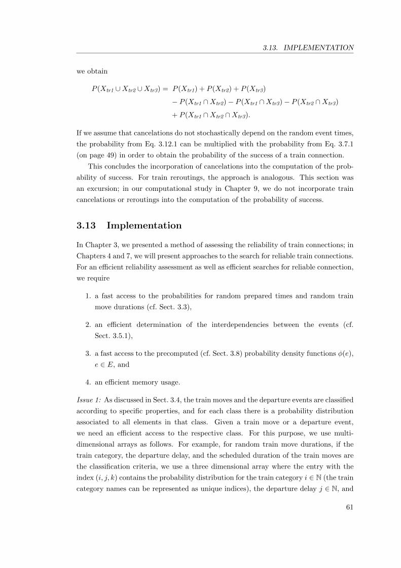
3.13. IMPLEMENTATION
we obtain
P (Xtr1 ∪Xtr2 ∪Xtr3) = P (Xtr1) + P (Xtr2) + P (Xtr3)
− P (Xtr1 ∩Xtr2)− P (Xtr1 ∩Xtr3)− P (Xtr2 ∩Xtr3)
+ P (Xtr1 ∩Xtr2 ∩Xtr3).
If we assume that cancelations do not stochastically depend on the random event times,
the probability from Eq. 3.12.1 can be multiplied with the probability from Eq. 3.7.1
(on page 49) in order to obtain the probability of the success of a train connection.
This concludes the incorporation of cancelations into the computation of the prob-
ability of success. For train reroutings, the approach is analogous. This section was
an excursion; in our computational study in Chapter 9, we do not incorporate train
cancelations or reroutings into the computation of the probability of success.
3.13 Implementation
In Chapter 3, we presented a method of assessing the reliability of train connections; in
Chapters 4 and 7, we will present approaches to the search for reliable train connections.
For an efficient reliability assessment as well as efficient searches for reliable connection,
we require
1. a fast access to the probabilities for random prepared times and random train
move durations (cf. Sect. 3.3),
2. an efficient determination of the interdependencies between the events (cf.
Sect. 3.5.1),
3. a fast access to the precomputed (cf. Sect. 3.8) probability density functions φ(e),
e ∈ E, and
4. an efficient memory usage.
Issue 1: As discussed in Sect. 3.4, the train moves and the departure events are classified
according to specific properties, and for each class there is a probability distribution
associated to all elements in that class. Given a train move or a departure event,
we need an efficient access to the respective class. For this purpose, we use multi-
dimensional arrays as follows. For example, for random train move durations, if the
train category, the departure delay, and the scheduled duration of the train moves are
the classification criteria, we use a three dimensional array where the entry with the
index (i, j, k) contains the probability distribution for the train category i ∈ N (the train
category names can be represented as unique indices), the departure delay j ∈ N, and
61

CHAPTER 3. RELIABILITY ASSESSMENT
the scheduled train move duration k ∈ N. For random preparation times the procedure
is analogous.
Issues 2–4: For the latter three questions (see above), we propose two solutions. Each of
them has its weaknesses and strengths; the suitable method should be chosen depending
on the use case as will be discussed. The first solution is extending the graph model
that represents the timetable (cf. Sect. 2.1); we discuss this solution in Sect. 3.13.1. The
second solution is introducing a separate dependency graph as explained in Sect. 3.13.2.
In Sect. 3.13.3, we discuss dropping negligible probabilities in order to reduce the
width of the probability distributions. Finally, in Sect. 3.13.4, we discuss the imple-
mentation of the queue specified in Sect. 3.8.2.2.
3.13.1 Extension of the Graph Model
As discussed in Sect. 2.1, the timetable can be represented as a time-expanded or a
time-dependent graph. Each of these graph models can be extended in order to provide
an access to the functions φ(e), e ∈ E, as well as to the interdependencies between the
events; the access can be facilitated in constant time. This approach is designed to
be combined with the approach from Sect. 3.8.2 to compute all functions φ(e), e ∈ E,
in pre-processing. The memory usage by this approach is higher compared to the
approach that will be discussed in Sect. 3.13.2. However, it is the best solution if a fast
access to the functions φ(e), e ∈ E, is required as for the approach from Chapter 5.
In the following, we explain how we extend the time-expanded graph model. Such an
extension is possible for the time-dependent graph model as well but it is not in the
focus of this work.
Extending the time-expanded graph model Each departure and arrival node,
representing an event e ∈ E, additionally stores the function φ(e) so that this function
can be accessed in constant time.
Moreover, we facilitate an efficient determination of the interdependencies between
the events (cf. Sect. 3.5.1) as follows. Each arrival node varr has an incoming train
edge (vdep, varr), and, therefore, it knows the departure node vdep on which it depends.
On the other side, each departure node vs,trdep ∈ Vdep knows the arrival node vs,tr
arr via
the incoming dwell edge. These dependencies can be efficiently extracted from the
time-expanded graph model.
On the other side, for each departure node vsdep ∈ Vdep, we need to determine via
the change layer at the station s the set of the arrival events of other trains for which
vsdep waits (cf. the set Edepend
arr (edep) in Sect. 3.5.1.1). In order to facilitate an access
from a departure node vdep to the arrival nodes for which vdep waits, we add to the
graph feeder edges. Let vsarr and vs
dep represent the events esarr ∈ Earr and es
dep ∈ Edep
62

3.13. IMPLEMENTATION
respectively. We create a feeder edge from vsarr to vs
dep if max wait(esarr, e
sdep) is greater
than zero. The feeder edges of a departure node are stored as its incoming edges so
that they can be accessed from the departure node in constant time. Hence, given an
event, its dependencies can be looked up in constant time. We evaluate this approach
in Sect. 9.2.1.
3.13.2 Dependency Graph
We now discuss a method with a significantly lower memory usage compared to the
graph extension from Sect. 3.13.1. The access to the functions φ(e), e ∈ E, and the
interdependencies between the events can be performed using a hash structure or a
binary search tree. This method is designed to be combined with the hybrid approach
to computing probability density functions as presented in Sect. 3.8.3. We recommend
this combination for very large timetables where only a small proportion of the events
has complex interdependencies. According to the timetables for the German train
network including local public transport, this hybrid approach is suitable. The pre-
processing step ignores a large number of events of buses and streetcars which usually
do not wait. We will evaluate this approach in Sect. 9.2.1. Below, we present the
details.
Note: The dependency graph approach from this section can also be combined with the
method of computing the probability density functions in pre-processing (cf. Sect. 3.8.2);
however, in this case, it would result in a memory usage higher than the graph extension
method (cf. Sect. 3.13.1), and, therefore, it would be pointless.
Definition of the dependency graph [MHS09] presented the dependency graph
model; based on this idea, we introduce a dependency graph that stores the functions
φ(e), e ∈ E, and the interdependencies between the events. It is defined as follows.
Let the set E′ ⊆ E comprise the following events:
• all events of each train tr ∈ TR where there is at least another train tr′ ∈ TR
which waits for tr at some station (according to the maximum waiting times from
Sect. 1.3), and
• all events of each train which waits for at least one other train at some station.
In our dependency graph, for each event e ∈ E′, there is a node in the graph. The
respective node for the event e stores the function φ(e).
In the dependency graph, for e, e′ ∈ E′, there is an edge from the node of e to
the node of e′ if the random event time of e′ depends on the random event time of
e as discussed in Sect. 3.5.1. More precisely, for each earr ∈ E′ of the train move
63

CHAPTER 3. RELIABILITY ASSESSMENT
(edep, earr) ∈ TM, in the dependency graph, there is an edge from the node representing
edep to the node representing earr. On the other side, for each edep ∈ E′, there is an
edge to the node representing edep from each node representing an event in Edependarr (e).
Each node knows its incoming and outgoing edges.
Hence, combined with the hybrid approach from Sect. 3.8.3, the dependency graph
comprises only those probability density functions which cannot be computed on-
demand efficiently.
Note: The graph that represents the timetable is not connected to the dependency graph;
they are two individual data structures.
Access to the nodes To access the function φ(e) or the dependencies of an event
e ∈ E, we need to search for the respective node in the dependency graph. If a node
for e exists in the dependency graph, it can be delivered; otherwise, φ(e) and the
dependencies are determined on-the-fly.
To find nodes in the dependency graph efficiently, we create a unique key for
each event; it can be derived from the data about the event which is available in the
timetable. For example, we use a combination of the train category, the train number,
the event type (departure or arrival), the scheduled event time, and the station of the
event. This key can be hashed or stored in a binary search tree. Using the key, we can
find the node of an event efficiently.
3.13.3 Negligible Probabilities
In order to manage numerical issues and reduce the number of elements in the supports
of the probability density functions φ(e), e ∈ E, we drop negligible probabilities as
follows. For each event e ∈ E, we regard a time t ∈ supp(φ(e)) as negligible if φ(e, t) < ε.
We drop a negligible t if t is outside the range of non-negligible times; that is, we drop
a negligible t unless there are non-negligible times t′ < t and t′′ > t for the same
event. The parameter ε is part of our experimental setting in Sect. 9.2.1 (cf. Negligible
probabilities).
3.13.4 The Queue
In this section, we discuss how the queue from Sect. 3.8.2.2 can be implemented. We
propose two variants: an implementation as a priority queue and an implementation
as a dial queue.
Implementation as a priority queue First, the queue can be realized as a priority
queue; in such a queue each element has a priority, and the operation pop always
64

3.14. CONCLUSION
delivers the element with the highest priority. Translated to our problem, the priority
of each element in the queue, that is a train move, equals the latest time in TIMES
minus the scheduled event time of the departure event of the train move; this ensures
that the operation pop delivers the train moves sorted by the scheduled event times
of their departure events in ascending order. If a heap is used as the backbone of the
priority queue, the complexity of each call of the operations push and pop is O(log n)
where n is the number of the elements in the queue.
Implementation as a dial queue Alternatively, the queue can be realized analogous
to the Dial’s implementation of the Dijkstra’s algorithm as discussed in [AMZ09]. More
precisely, the queue is an array of buckets; it contains a bucket for each time t ∈ TIMES.
The first and the last element in the array are the buckets for the earliest and the latest
time in TIMES respectively. The operation push inserts a train move (edep, earr) into
the bucket for the time sched(edep). For the operation pop, the queue contains a pointer
to the bucket with the earliest time that contains at least one element; the operation
pop delivers an element from this bucket, removes it from the bucket, and updates the
pointer if the bucket has become empty. Consequently, the operations push and pop
run in constant time.
3.14 Conclusion
In this chapter, we presented our method of assessing the reliability of train connections.
More precisely, we compute the probability of the success of each train connection;
the probability that—when taking the train connection—passengers can reach their
destination and the train connection does not break because of delays. Our method is
based on stochastic predictions for the departure and arrival events of trains (functions
φ(e), e ∈ E). The evaluations of our method in Sect. 9.3 will reveal that our reliability
assessments are realistic and widely accurate. However, the quality of our assessments
strongly depends on the quality of the input data such as the probability distributions
for the random durations of the train moves (cf. Sect. 10.1).
In this chapter, we also demonstrated efficient procedures of computing the func-
tions φ(e), e ∈ E, as well as updating them according to the current situation in the
railway network. We described how to store the computed probability density functions
and provide fast access to them.
In Sect. 9.3, we will see that our method can be applied to large train networks
such as those in Germany. The method is fast and efficient even for large timetables
that include short- and long-distance trains as well as local public transport such as
buses and streetcars.
65


Chapter 4
On-Time Arrival Guarantee
4.1 Introduction
In Chapter 3, we introduced our approach to assessing the probability of the success of
a train connection. We now address the search for journeys that are reliable regarding
disruptions in the timetable. In Chapters 4–8, we address relevant problems of travelers
and provide solutions for them.
In Sect. 1.2, we introduced a train connection as a sequence of train and walk
trips. Transfers in train connections can break due to delays. When a transfer in a
train connection breaks, the journey does not end for the passenger who has taken the
train connection; he/she continues the journey via an alternative continuation to the
destination.
Alternative continuations Given a train connection c = trip1, trip2, . . . , tripn (cf.
Sect. 1.2), an alternative continuation is a train connection c′ = trip′1, trip′2, . . . , trip′m
that fulfills the following two conditions:
1. The train connections c and c′ end at the same station, that is, the destination
station of the passenger.
2. The alternative continuation c′ starts at a station s that is visited by c as well.
Let es,tr2dep be the very first departure event of c′ at s. Moreover, let es,tr
arr denote
the arrival event of the train connection c at s. The activity (es,trarr , e
s,tr2dep ) is either
a dwell activity (if tr = tr2) or a transfer activity (if tr 6= tr2). In the case that c′
starts with a walk trip, its very first departure event is at a station s2 6= s, and
(es,trarr , e
s2,tr2dep ) is a transfer activity with a walk trip.
67
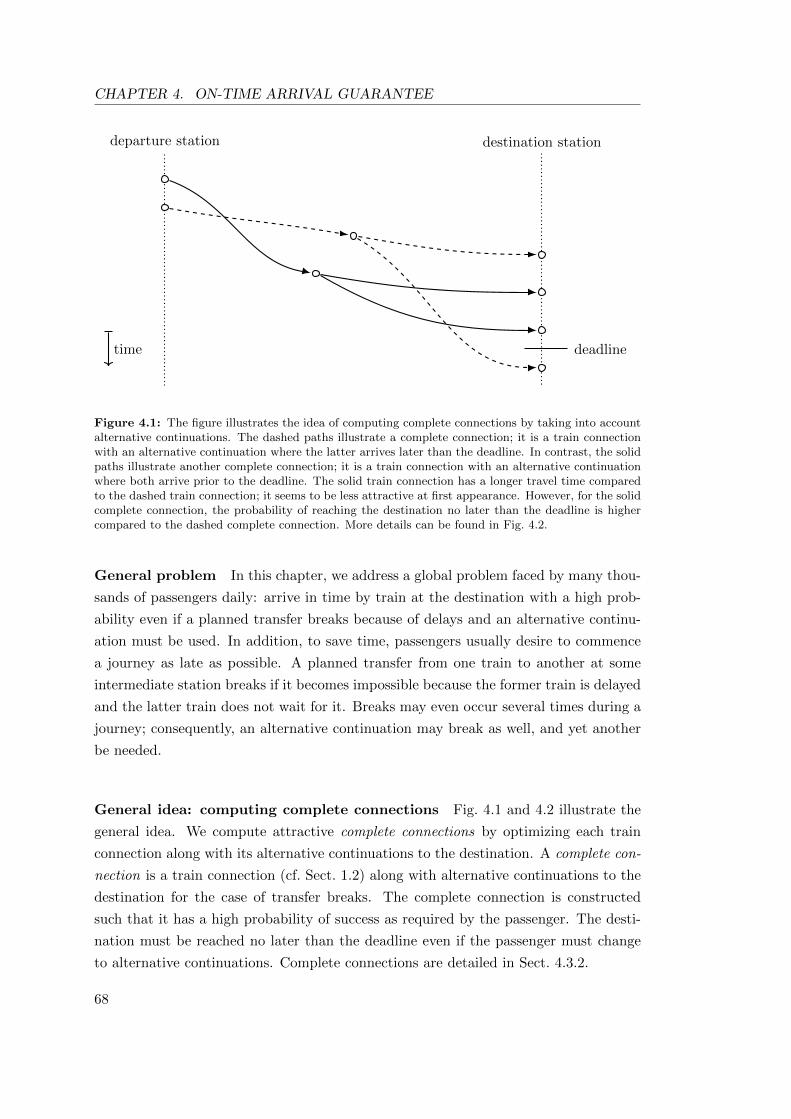
CHAPTER 4. ON-TIME ARRIVAL GUARANTEE
departure station destination station
deadlinetime
Figure 4.1: The figure illustrates the idea of computing complete connections by taking into accountalternative continuations. The dashed paths illustrate a complete connection; it is a train connectionwith an alternative continuation where the latter arrives later than the deadline. In contrast, the solidpaths illustrate another complete connection; it is a train connection with an alternative continuationwhere both arrive prior to the deadline. The solid train connection has a longer travel time comparedto the dashed train connection; it seems to be less attractive at first appearance. However, for the solidcomplete connection, the probability of reaching the destination no later than the deadline is highercompared to the dashed complete connection. More details can be found in Fig. 4.2.
General problem In this chapter, we address a global problem faced by many thou-
sands of passengers daily: arrive in time by train at the destination with a high prob-
ability even if a planned transfer breaks because of delays and an alternative continu-
ation must be used. In addition, to save time, passengers usually desire to commence
a journey as late as possible. A planned transfer from one train to another at some
intermediate station breaks if it becomes impossible because the former train is delayed
and the latter train does not wait for it. Breaks may even occur several times during a
journey; consequently, an alternative continuation may break as well, and yet another
be needed.
General idea: computing complete connections Fig. 4.1 and 4.2 illustrate the
general idea. We compute attractive complete connections by optimizing each train
connection along with its alternative continuations to the destination. A complete con-
nection is a train connection (cf. Sect. 1.2) along with alternative continuations to the
destination for the case of transfer breaks. The complete connection is constructed
such that it has a high probability of success as required by the passenger. The desti-
nation must be reached no later than the deadline even if the passenger must change
to alternative continuations. Complete connections are detailed in Sect. 4.3.2.
68
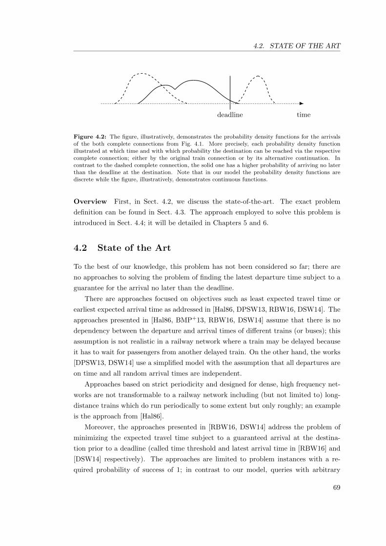
4.2. STATE OF THE ART
timedeadline
Figure 4.2: The figure, illustratively, demonstrates the probability density functions for the arrivalsof the both complete connections from Fig. 4.1. More precisely, each probability density functionillustrated at which time and with which probability the destination can be reached via the respectivecomplete connection; either by the original train connection or by its alternative continuation. Incontrast to the dashed complete connection, the solid one has a higher probability of arriving no laterthan the deadline at the destination. Note that in our model the probability density functions arediscrete while the figure, illustratively, demonstrates continuous functions.
Overview First, in Sect. 4.2, we discuss the state-of-the-art. The exact problem
definition can be found in Sect. 4.3. The approach employed to solve this problem is
introduced in Sect. 4.4; it will be detailed in Chapters 5 and 6.
4.2 State of the Art
To the best of our knowledge, this problem has not been considered so far; there are
no approaches to solving the problem of finding the latest departure time subject to a
guarantee for the arrival no later than the deadline.
There are approaches focused on objectives such as least expected travel time or
earliest expected arrival time as addressed in [Hal86, DPSW13, RBW16, DSW14]. The
approaches presented in [Hal86, BMP+13, RBW16, DSW14] assume that there is no
dependency between the departure and arrival times of different trains (or buses); this
assumption is not realistic in a railway network where a train may be delayed because
it has to wait for passengers from another delayed train. On the other hand, the works
[DPSW13, DSW14] use a simplified model with the assumption that all departures are
on time and all random arrival times are independent.
Approaches based on strict periodicity and designed for dense, high frequency net-
works are not transformable to a railway network including (but not limited to) long-
distance trains which do run periodically to some extent but only roughly; an example
is the approach from [Hal86].
Moreover, the approaches presented in [RBW16, DSW14] address the problem of
minimizing the expected travel time subject to a guaranteed arrival at the destina-
tion prior to a deadline (called time threshold and latest arrival time in [RBW16] and
[DSW14] respectively). The approaches are limited to problem instances with a re-
quired probability of success of 1; in contrast to our model, queries with arbitrary
69

CHAPTER 4. ON-TIME ARRIVAL GUARANTEE
values for the required probability of success are not supported (cf. Sect. 4.3.1). In ad-
dition, the approach presented in [RBW16] requires several minutes per query even for
the very small dataset which was evaluated in that work. Thus, the approach does not
scale to large train networks such as those from our computational study in Sect. 9.4.
The approach presented in [GKMH+11, GSS+14] assumes a subset of all delay
scenarios that can occur in the train network. A transfer is called robust if it never
breaks in any delay scenario in the assumed subset. Based on this definition, two
approaches are introduced: strict robustness and light robustness. The strict robustness
approach delivers paths that solely contain robust transfers. In contrast, the light
robustness approach delivers a path with a minimum number of non-robust transfers,
subject to a maximal increase of travel time compared to the nominal solution (in
those works, the nominal solution is the connection with the earliest arrival time at the
destination).
In contrast to our objective, strict robustness results in travel times which are much
longer than travel times obtained by our approach (cf. Fig. 6 in [GSS+14]). On the
other hand, light robustness delivers paths with non-robust transfers for a significant
number of queries. Hence, a probability of success cannot be guaranteed with the
second approach—even for the seriously restricted delay scenarios that are evaluated
in [GKMH+11, GSS+14].
Another robustness approach has been presented in [GHMH+13]. The response
times of that approach are prohibitive in our real-world setting; that is, several minutes
per query for the seriously restricted delay scenarios that are evaluated in [GHMH+13].
Approaches for networks without a timetable (for example for road networks) such
as presented in [FN06, NBK06, SBB11, SBB12, PSG13, FR98, Pre98, NPA04, NPA06,
AJ14] are evidently not transferable to our problem; in contrast to a railway network,
they can use each graph arc at any time, and they do not deal with the issue that
transfers can break due to delays. The model presented in [Pre98, NPA04, NPA06]
requires a hyper-arc for each possible value for the random variable of each node. In a
timetable based network like ours, this would blow up the graph size prohibitively.
The authors of [MHS09] presented an approach to accompanying a passenger during
his/her journey by providing him/her alternative continuations in case of train connec-
tion breaks. In Sect. 7.1.3 and 9.4.6, we will compare this approach to our approach
from this work; we will see that this alternative approach often fails to deliver optimal
solutions.
Publication of the author A manuscript has already been submitted to the journal
Transportation Science (see [KSW17]); it is a short version of the content presented in
Chapters 3–6, Sect. 7.1, and Sect. 9.4. In the mentioned chapters and sections, there
70

4.3. PROBLEM DEFINITION
are phrases and wordings which also appear in [KSW17]. A former version of that
submission had been published in [KSW14].
4.3 Problem Definition
In this section, we precisely define the problem introduced in Sect. 4.1.
4.3.1 Input and Queries
Input The input is a timetable, the function φ(e) for each event e ∈ E, the functions
θ(tm, tdep) for each tm ∈ TM and each tdep ∈ TIMES, the functions ξ(edep) for each
edep ∈ Edep, and a query.
Queries A query q comprises
• a departure station where the journey starts, denoted by dep st(q) ∈ S,
• a destination station where the journey ends, denoted by dest st(q) ∈ S,
• a deadline when the passenger wants to arrive at the latest at dest st(q), denoted
by deadline(q) ∈ TIMES, and
• a required probability of success, denoted by ρreq(q) ∈ [0, 1] ⊂ R, which might be
close to 1 in real-world settings. This parameter can be chosen by the passenger
or automatically set by a timetable information system.
4.3.2 Outcomes: Complete Connections
In Sect. 4.1, we introduced complete connections. An outcome for a query is a complete
connection; that is,
• a train connection from dep st(q) to dest st(q),
• along with alternative continuations to dest st(q) for all points where the train
connection may break,
• plus alternative continuations for these alternative continuations, and so on.
More precisely, for each situation that may occur during the journey, the outcome
contains a precomputed instruction what to do next.
This definition of complete connections is sufficient to understand the rest of this
chapter; the exact definition of complete connections is presented in Sect. 5.1. Complete
connections have relevant properties which we introduce here and precisely define in
Sect. 5.5.
71

CHAPTER 4. ON-TIME ARRIVAL GUARANTEE
Probability of the success of a complete connection For a complete connec-
tion c, computed for a query q, the value ρ(c) denotes the probability of the success of c;
the probability that, when taking c, the passenger is able to travel from dep st(q) to
dest st(q) up to deadline(q). A complete connection c is called feasible if ρ(c) ≥ ρreq(q);
otherwise it is called infeasible. We discuss the computation of the probability of the
success of a complete connection in Chapter 5.
The probability of the success of a complete connection can be guaranteed only at
the time when it is computed. Whenever the network state has changed—due to delays
or other real-time incidents (cf. Sect. 1.3)—the probability of the success of a formerly
computed complete connection could be affected. We address this issue in Chapter 6.
Note: In Chapter 3, we used the terms “feasible” and “infeasible” for transfers and train
connections in a different context and with a different meaning. There, we addressed
the feasibility according to the timetable and the real times.
Note: In Sect. 3.7, we introduced the probability of the success of train connections. The
probability of the success of a complete connection cannot be computed exactly as for a
train connection since the former has a different structure and could contain multiple
alternative continuations. However, the computation of the probability of the success of
a complete connection is based on definitions and formulas from Chapter 3.
Scheduled departure time of a complete connection For a complete connec-
tion c, the value dep time(c) ∈ TIMES denotes the scheduled departure time of c at
the departure station dep st(q) of the query q. In Sect. 5.1.1, we will specify this value
more precisely.
Expected number of transfers For a complete connection c, this is the expected
number of transfers which are necessary in order to travel from dep st(q) to dest st(q)
when taking c. The computation is addressed in Sect. 5.3.4.
Expected arrival time For a complete connection c, this is the expected arrival
time at dest st(q) when taking c. The computation is addressed in Sect. 5.4.2.
Expected travel time For a complete connection, this value is the time difference
between the expected arrival time at dest st(q) and the scheduled departure time at
dep st(q). The computation is addressed in Sect. 5.4.2.
72

4.3. PROBLEM DEFINITION
4.3.3 Exact Problem Definition
In Sect. 4.3.3.1, we present the exact problem definition and specify the optimal out-
come for a query q. Moreover, in Sect. 4.3.3.2–4.3.3.5, we define different variants of
the problem with different objective functions. The problem from Sect. 4.3.3.1 is the
main problem addressed in Chapters 4–6 and evaluated in Sect. 9.4. The other vari-
ants are introduced in order to demonstrate that our approach to computing complete
connections can be adjusted in order to solve relevant related problems.
Set C(q) For all problem variants, the optimal outcome is chosen from the set C(q);
it comprises all (not necessarily feasible) complete connections existing for a query q.
For the following definitions of the objective functions of the problem variants, we use
the operators “arg max” and “arg min”; given a set of arguments (complete connections
in our use case) and a function f , the operators “arg max” and “arg min” deliver the
arguments that maximize and minimize the function output respectively; ties are broken
arbitrarily.
4.3.3.1 Latest Departure Subject to Arrival Guarantee
The most interesting problem is to find a complete connection such that the scheduled
departure time at dep st(q) is as late as possible subject to the guarantee that dest st(q)
is reached no later than deadline(q) with a probability of at least ρreq(q). Consequently,
subject to the required probability of success ρreq(q), the departure time at dep st(q) has
to be maximized. Formally, the optimal outcome o is a complete connection described
by the following objective function:
Cfeasible(q) = { c ∈ C(q)∣∣ ρ(c) ≥ ρreq(q) },
o = arg max { dep time(c)∣∣ c ∈ Cfeasible(q) }. (4.3.1)
Degrees of freedom More than one element in the set Cfeasible(q) could maximize
the objective function from Eq. 4.3.1. Hence, our approach for the search for optimal
complete connections has degrees of freedom. In such a case, we could optimize a
secondary criterion like the expected number of transfers, the expected travel time,
or a combination of them. We will address this issue in Sect. 5.3.4 and 5.4.2. These
tie-break rules are applicable to all problem variants from Sect. 4.3.3.
4.3.3.2 Maximum Probability of Success
Another variant of the problem from Sect. 4.3.3.1 is to find a complete connection that
maximizes the probability of success. Among all complete connections which maximize
73

CHAPTER 4. ON-TIME ARRIVAL GUARANTEE
the probability of success, we are interested in the complete connection with the latest
scheduled departure time at dep st(q). Formally, the optimal outcome o is a complete
connection that is described by the following objective function:
Cmax(q) = arg max set { ρ(c)∣∣ c ∈ C(q) },
o = arg max{
dep time(c)∣∣ c ∈ Cmax(q)
}. (4.3.2)
4.3.3.3 On-Trip Scenario at a Station
We address a relevant problem that occurs in an on-trip scenario where the passenger
has already started traveling, he/she already waits at a station at the time ontrip time ∈TIMES (for example because his original train connection is broken at that station),
and is looking for the complete connection with the highest probability of arriving at
dest st(q) no later than deadline(q).
We seek the complete connection c with the maximum probability of success ρ(c)
such that dep time(c) is not earlier than ontrip time. The optimal outcome o is a
complete connection that is described by the following objective function:
Contrip(q) = { c ∈ C(q)∣∣ dep time(c) ≥ ontrip time },
o = arg max { ρ(c)∣∣ c ∈ Contrip(q) }. (4.3.3)
4.3.3.4 On-Trip Scenario in a Train
We address another on-trip scenario; the passenger is in a train; more precisely, he/she
is on the train move tm ∈ TM, and seeks for a complete connection in order to
travel to dest st(q). Accurately, we seek the complete connection c that starts with
the train move tm, and maximizes the probability of arriving at dest st(q) no later than
deadline(q). Let Ctm(q) ⊂ C(q) denote the set of all (not necessarily feasible) complete
connections that start with the train move tm. Formally, the optimal outcome o is a
complete connection described by the following objective function:
o = arg max { ρ(c)∣∣ c ∈ Ctm(q) }. (4.3.4)
4.3.3.5 Minimum Expected Travel Time
Among all complete connections which guarantee a probability of success of 1, we
seek the complete connection that has the minimum expected travel time and a sched-
uled departure time in the time interval [earliest dep time, latest dep time]. In contrast
to the problem definitions in Sect. 4.3.3.1–4.3.3.3, the deadline plays no role; we set
74

4.4. TWO-STAGE APPROACH
deadline(q) = +∞. Formally, the objective function is as follows:
Cinterval(q) = { c ∈ C(q)∣∣ dep time(c) ≥ earliest dep time ∧
dep time(c) ≤ latest dep time },
Creliableinterval(q) = { c ∈ Cinterval(q)
∣∣ ρ(c) = 1 },
o = arg min { exp travel time(c)∣∣ c ∈ Creliable
interval(q) }. (4.3.5)
4.4 Two-Stage Approach
We propose a two-stage approach to solving the problem from Sect. 4.3, respectively,
with two related software components:
1. Booking stage: To plan the journey in advance, the search component computes
the optimal outcome (a complete connection as introduced in Sect. 4.3.2 and
precisely defined in Sect. 5.1) so that the required probability of success ρreq(q) is
met given all information available at the time of planning. For each situation that
may occur while traveling, the search component computes the best instruction
concerning what to do next.
2. Journey : While traveling, the passenger is guided by the travel guidance compo-
nent. This component interprets the instructions computed by the search com-
ponent. In short, whenever the passenger waits at a station, the travel guidance
component suggests which train to take next. Whenever the passenger sits in a
train, it suggests what to do at the very next halt: to stay in the train or to leave
it.
In Chapter 5, we introduce our approach to the search component. The travel guidance
component is detailed in Chapter 6.
This two-stage approach has become established in most timetable information sys-
tems. They usually consist of a back-end component that is responsible for processing
the search query, and a front-end component that presents the results to the user. We
correspondingly follow this two-stage approach. In addition, we generalize the second
stage by introducing the travel guidance component. In addition to a comprehensive
visualization of complete connections, by the travel guidance component, we address
another relevant problem: as announced in Sect. 4.3.2, the probability of the success
of a complete connection can be guaranteed only at the time of its computation. The
travel guidance component is responsible for preserving the optimality of complete
connections even after changes to the train network due to delays and other real-time
incidents (cf. Sect. 1.3). This is obtained by updating the complete connections as
discussed in Chapter 6.
75

Chapter 5
Optimal Complete Connections
As detailed in Sect. 4.4, we follow a two-stage approach in order to compute optimal
outcomes to the problem from Sect. 4.3. The second stage, travel guidance, is presented
in Chapter 6. The first stage is realized by the search component presented in this
chapter. The input for the search component is as specified in Sect. 4.3.1 (cf. Input).
Given a query, the search component computes the optimal outcome according to the
problem definition from Sect. 4.3.2. We first introduce the probability of success for
an event in the timetable; the search for optimal complete connections is based on the
computation of this probability for events in the set E.
Probability of success ρ(e) for an event Given a query q, the probability of
success ρ(e) for an event e ∈ E is the probability that from e the destination station
dest st(q) can be reached no later than deadline(q). In Sect. 5.3.2, we explain how this
probability is computed.
Overview First, in Sect. 5.1, we precisely define the outcome of the search compo-
nent. In Sect. 5.2, we address the exponential size of the solution space, and abstractly
explain our approach to computing and retrieving optimal complete connections. This
abstract description is detailed in the subsequent sections.
In Sect. 5.3 and 5.4, we present two different recursive functions that compute the
probability of success for events in the timetable as well as the best instruction to
continue the journey for each situation that may occur when traveling (cf. Sect. 4.4).
These recursive functions are later employed to compute optimal complete connections.
The problem variants from Sect. 4.3.3.1–4.3.3.4 can be solved by the recursive function
from Sect. 5.3 unless the travel time must be minimized as a secondary criterion (cf.
Sect. 4.3.3.1). In the latter case, the function from Sect. 5.4 should be applied. Analo-
gously, the problem variant from Sect. 4.3.3.5 can be solved only by the function from
Sect. 5.4.
77

CHAPTER 5. OPTIMAL COMPLETE CONNECTIONS
In Sect. 5.5, we precisely define relevant properties of complete connections, which
have already been introduced in Sect. 4.3.2. In addition, we discuss how they are
defined according to the values computed by employing the recursive functions from
Sect. 5.3 and 5.4. Up to Sect. 5.6, we omit the details concerning the incorporation of
walk trips into the computation of complete connections; in that section, these details
are explained.
In Sect. 5.7, we translate the recursive functions from Sect. 5.3 and 5.4 into a dy-
namic programming approach. This approach delivers the optimal complete connection
for each query. After that, in Sect. 5.8, we demonstrate a significant performance im-
provement of our dynamic programming approach (from Sect. 5.7); it is obtained by a
restriction of the computations to events which are actually relevant for the query. We
finally present in Sect. 5.9 an efficient algorithm for the computation of optimal com-
plete connections; this algorithm is designed for the problem variant from Sect. 4.3.3.1
(cf. Latest Departure Subject to Arrival Guarantee).
In Sect. 5.10, we discuss the asymptotic complexity of the approaches to the search
component. Then, in Sect. 5.11, we discuss heuristics which could improve the perfor-
mance of the search component. In Sect. 5.12, we briefly address a parallelization of the
search component. We provide details on our implementation of the search component
in Sect. 5.13. Finally, this chapter is concluded in Sect. 5.14.
5.1 Exact Definition of Complete Connections
Fig. 5.1 (on page 79) illustrates a complete connection. In Sect. 4.1–4.4, we introduced
a complete connection as a train connection, from dep st(q) to dest st(q) of a query q,
along with alternative continuations to dest st(q). For every situation that can occur
while traveling, a complete connection contains an instruction what to do next. More
precisely, a complete connection starts with a train move departing from dep st(q)—as
will be discussed in Sect. 5.1.1—and, from then on, it is based on arrival events. After
the arrival at each station visited during the journey, by taking into account the arrival
time, the complete connection contains an instruction concerning how to continue the
journey towards the destination. Formally, this instruction is a departure event, and is
introduced in Sect. 5.1.2.
5.1.1 Initial Departure Event
A relevant element of each complete connection is its initial departure event. Each
complete connection, computed for a query q, starts with a specific departure event
at dep st(q). The other way round, for each departure event einitdep ∈ E
dep st(q)dep , a set
of complete connections can be computed which start with einitdep unless there is no
78
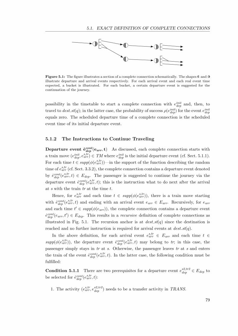
5.1. EXACT DEFINITION OF COMPLETE CONNECTIONS
Figure 5.1: The figure illustrates a section of a complete connection schematically. The shapes andillustrate departure and arrival events respectively. For each arrival event and each real event timeexpected, a bucket is illustrated. For each bucket, a certain departure event is suggested for thecontinuation of the journey.
possibility in the timetable to start a complete connection with einitdep and, then, to
travel to dest st(q); in the latter case, the probability of success ρ(einitdep) for the event einit
dep
equals zero. The scheduled departure time of a complete connection is the scheduled
event time of its initial departure event.
5.1.2 The Instructions to Continue Traveling
Departure event econtdep (earr, t) As discussed, each complete connection starts with
a train move (einitdep, e
s,trarr) ∈ TM where einit
dep is the initial departure event (cf. Sect. 5.1.1).
For each time t ∈ supp(φ(es,trarr))—in the support of the function describing the random
time of es,trarr (cf. Sect. 3.3.2), the complete connection contains a departure event denoted
by econtdep (es,tr
arr , t) ∈ Edep. The passenger is suggested to continue the journey via the
departure event econtdep (es,tr
arr , t); this is the instruction what to do next after the arrival
at s with the train tr at the time t.
Hence, for es,trarr and each time t ∈ supp(φ(es,tr
arr)), there is a train move starting
with econtdep (es,tr
arr , t) and ending with an arrival event earr ∈ Earr. Recursively, for earr
and each time t′ ∈ supp(φ(earr)), the complete connection contains a departure event
econtdep (earr, t
′) ∈ Edep. This results in a recursive definition of complete connections as
illustrated in Fig. 5.1. The recursion anchor is at dest st(q) since the destination is
reached and no further instruction is required for arrival events at dest st(q).
In the above definition, for each arrival event es,trarr ∈ Earr and each time t ∈
supp(φ(es,trarr)), the departure event econt
dep (es,trarr , t) may belong to tr; in this case, the
passenger simply stays in tr at s. Otherwise, the passenger leaves tr at s and enters
the train of the event econtdep (es,tr
arr , t). In the latter case, the following condition must be
fulfilled:
Condition 5.1.1 There are two prerequisites for a departure event es2,tr2dep ∈ Edep to
be selected for econtdep (es,tr
arr , t):
1. The activity (es,trarr , e
s2,tr2dep ) needs to be a transfer activity in TRANS.
79

CHAPTER 5. OPTIMAL COMPLETE CONNECTIONS
2. The following constraint needs to be fulfilled:
t+ min dur(es,trarr , e
s2,tr2dep ) ≤ sched(es2,tr2
dep ) + max wait(es,trarr , e
s2,tr2dep ).
In words, Condition 5.1.1 ensures that the passenger will be able to transfer from tr
to tr2 if the former arrives at s at the time t. Depending on whether s and s2 are the
same station or not, the activity (es,trarr , e
s2,tr2dep ) is a transfer without or with a walk trip
respectively.
Case of failure In a complete connection, for some arrival event es,trarr and some
time t ∈ supp(φ(es,trarr)), the value econt
dep (es,trarr , t) can be void. The complete connection
consequently does not provide any instruction to continue traveling after the arrival
at s with the train tr at the time t. The journey could get stuck at the station s. The
probability of the success of such a complete connection is consequently lower than 1.
5.2 The Search Approach
In Sect. 5.1, we exactly defined the structure of the outcome of our search component;
a complete connection. In this section, we address the problem of finding the optimal
complete connection for each query. We first demonstrate that the solution space is
exponentially large but, fortunately, can be reduced to a manageable size without loss
of optimality. We then discuss how all complete connections in the reduced solution
space can be retrieved. From those complete connections, the search component finally
delivers the optimal one.
5.2.1 The Solution Space
Exponential size In Sect. 4.3.3, we introduced the set C(q) of all (not necessarily
feasible) complete connections existing for a query q; this set builds the search space.
For the problem variant from Sect. 4.3.3.1 (cf. Latest Departure Subject to Arrival
Guarantee), the feasibility is required; that is, satisfying the required probability of
success ρreq(q). The set of all feasible complete connections is called the solution space;
it is a subset of the search space. Both of these sets can be exponentially large; an
explanation follows.
Given an arrival event earr ∈ Earr, let n ∈ N0 denote the number of the departure
events which can be selected for econtdep (earr, t) for some time t ∈ supp(φ(earr)). In
addition, we define k = |supp(φ(earr))|. There are up to nk different possibilities to
set the values econtdep (earr, t) for all t ∈ supp(φ(earr)). Consequently, the search space—
the set C(q)—can be exponentially large in the number of the events in E and the
80

5.2. THE SEARCH APPROACH
cardinalities of the supports of the functions φ(e), e ∈ E. Moreover, according to
Eq. 4.3.1 (on page 73), for a query q with deadline(q) = +∞, the solution space equals
the search space, and could also be exponentially large.
Reducing the solution space The objective functions in our problem definition
from Sect. 4.3.3 are based on the set C(q). In order to find the optimal complete
connection for a query efficiently, we need to reduce the solution space to a manageable
size. More precisely, we find a subset of C(q) which has a manageable size and still
contains the optimal complete connection. This subset is denoted by Cbest(q) ⊆ C(q),
and is defined as follows.
Set Cbest(q) First, for each departure event einitdep ∈ E
dep st(q)dep , there is at most one
complete connection in the set Cbest(q) ⊆ C(q) with einitdep as the initial departure event
(cf. Sect. 5.1.1); there is no complete connection for einitdep if ρ(einit
dep) equals zero. Thus,
the cardinality of the set Cbest(q) is lower than or equal to |Edep st(q)dep |.
Second, each complete connection c ∈ Cbest(q) with the initial departure event
einitdep ∈ E
dep st(q)dep is constructed such that the condition
ρ(einitdep) = ρ(c) ≥ ρ(c′)
is satisfied for c and each complete connections c′ /∈ Cbest(q) with the initial departure
event einitdep. In words, c is the complete connection by which the maximum probability of
success can be obtained given that the passenger starts the journey with einitdep. According
to the problem definitions from Sect. 4.3, this definition ensures that Cbest(q) contains
the optimal complete connection for the query q—in addition to suboptimal ones.
Probability of the success of each complete connection in Cbest(q) Recall the
definition of probability of success for complete connections and events, respectively, in
Sect. 4.3.2 and at the beginning of Chapter 5. According to the definition of Cbest(q),
for each complete connection c ∈ Cbest(q), the probability of success ρ(c) equals the
probability of success ρ(einitdep) of the initial departure event einit
dep of c.
5.2.2 Computing the Optimal Complete Connection
Computing the complete connections in Cbest(q) The complete connections in
the set Cbest(q) are computed as follows. In brief, for each situation that may occur
while traveling, the search component computes the best instruction concerning how to
continue the journey. More precisely, for each arrival event earr ∈ Earr and each time
t ∈ supp(φ(earr)), we select a departure event for econtdep (earr, t) (cf. Sect. 5.1.2) such that
81

CHAPTER 5. OPTIMAL COMPLETE CONNECTIONS
the following probability is maximized : the probability of reaching dest st(q) no later
than deadline(q) given that
• earr takes place at the time t and,
• from earr, the journey is continued via econtdep (earr, t).
If there is no departure event that can be selected for econtdep (earr, t), this value is set to
void ; we detail this case below (cf. Case of failure). Hence, the complete connections
in the set Cbest(q) can be retrieved once the best values for econtdep (earr, t) are computed
for each earr ∈ Earr and each time t ∈ supp(φ(e)).
This brief description of our approach to computing the optimal complete connec-
tion will be detailed in the rest of this chapter. In Sect. 5.3 and 5.4, we present two
different recursive functions that compute the values econtdep (earr, t) as described above.
Moreover, for each departure event einitdep ∈ E
dep st(q)dep , the probability of success ρ(einit
dep)
can be computed by those recursive functions.
Note: In Sect. 5.8, we will see that the search component need not compute the value
econtdep (earr, t) actually for each arrival event earr ∈ Earr. Without loss of optimality, the
computations can be restricted to a subset of all events which we call “relevant events”.
The optimal complete connection Once the complete connections in Cbest(q) are
retrieved, among them, the optimal complete connection is selected and delivered as the
outcome of the search component. It is the complete connection from the set Cbest(q)
that optimizes the respective objective function from Eq. 4.3.1–4.3.5 (cf. Sect. 4.3.3)
depending on the problem variant. Hence, in each of the objective functions, we can
safely replace C(q) by Cbest(q) as already discussed in Sect. 5.2.1. The outcome of the
search component will be void if the set Cfeasible(q), Cmax(q), Contrip(q), Ctm(q), and
Creliableinterval(q) from Eq. 4.3.1–4.3.5, respectively, is empty.
The objective functions from Eq. 4.3.1–4.3.5 require two properties of each com-
plete connection c: its scheduled departure time dep time(c) and its probability of
success ρ(c). Let einitdep ∈ E
dep st(q)dep denote the initial departure event of c. We obtain
dep time(c) = sched(einitdep) and ρ(c) = ρ(einit
dep).
Case of failure As addressed in Sect. 5.1.2 (cf. Case of failure), for an arrival event
earr ∈ Esarr and a time t ∈ supp(φ(earr)), whenever no departure event can be found
for econtdep (earr, t), the journey may get stuck at s. The value econt
dep (earr, t) is void ; it
indicates that an arrival via earr at the time t is too late, and there is no chance to
reach dest st(q) no later than deadline(q). Consequently, the probability of success ρ(c)
of each complete connection c that contains earr is less than 1.
82

5.3. COMPUTATION OF INSTRUCTIONS AND PROBABILITIES
If the value econtdep (earr, t) is void, and the passenger indeed arrives via earr at the time
t, our search component does not provide any instruction to continue the journey. In
such a case, the passenger is suggested to start a new query q with a value for deadline(q)
that is later than the original deadline since the latter cannot be met anymore. In this
situation, the problem variant from Sect. 4.3.3.3 (cf. On-Trip Scenario at a Station) is
in demand.
5.3 Computation of Instructions and Probabilities
In Sect. 5.2.2, we provided an overview of our approach to computing the optimal
complete connection. Recall that, for each arrival event earr ∈ Earr and each time
t ∈ supp(φ(earr)), we compute the best instruction concerning how to continue the
journey. More precisely, for econtdep (earr, t), we find a departure event such that the
following probability is maximized : the probability of reaching dest st(q) no later than
deadline(q) given that
• earr takes place at the time t and,
• from earr, the journey is continued via econtdep (earr, t).
In this section, we present a recursive function that computes the best departure event
for econtdep (earr, t) as described above. Moreover, the probability of success ρ(e) for each
e ∈ E can be computed by our recursive function. First, in Sect. 5.3.1, we introduce
the set of successor events of each event; from that set we always select the best event
to continue the journey. We then present our recursive function in Sect. 5.3.2. The
selection of the best departure event to continue the journey follows in Sect. 5.3.3.
From Sect. 4.3.3.1, recall that our search component has degrees of freedom so that
secondary criteria can be optimized; we will introduce an optimization of the expected
number of transfers in Sect. 5.3.4.
Note: The recursive function from this section optimizes the number of transfers as
a secondary criterion. In Sect. 5.4, we will present another recursive function which
additionally facilitates an optimization of the travel time as a secondary criterion. In
fact, that recursive function is an extension of the recursive function from this section.
Note: In Sect. 5.7, we will translate the recursive function from this section into a
dynamic programming approach by which we compute the complete connections in the
set Cbest(q) (cf. Sect. 5.2).
83

CHAPTER 5. OPTIMAL COMPLETE CONNECTIONS
5.3.1 Set of Successor Events
Set Esucc(e, t) For each event e ∈ E and each time t ∈ supp(φ(e)), the set of successor
events comprises each event e′ ∈ E where, from e, the journey can be immediately
continued via e′ given that e takes place at the time t; we denote this set by Esucc(e, t).
More precisely, for each departure event es,trdep ∈ Edep, the set Esucc(es,tr
dep, t) trivially
contains the arrival event es2,trarr of the train move (es,tr
dep, es2,trarr ) ∈ TM. On the other
hand, for each arrival event es,trarr ∈ Earr, the set Esucc(es,tr
arr , t) ⊆ Edep comprises
• the departure event es,trdep ∈ E
sdep of the dwell activity (es,tr
arr , es,trdep) ∈ DW—unless
es,trarr is the very last arrival event of tr—as well as
• each departure event in the set{es2,tr2
dep ∈ Edep
∣∣∣ (es,trarr , e
s2,tr2dep ) ∈ TRANS ∧
t+ min dur(es,trarr , e
s2,tr2dep ) ≤
sched(es2,tr2dep ) + max wait(es,tr
arr , es2,tr2dep )
};
the latter set fulfills Condition 5.1.1 (on page 80).
For each event at the destination of the query, the set of successor events is empty.
Note: The departure event econtdep (earr, t) is chosen from the set Esucc(e, t) of the successor
events of earr as will be detailed in Sect. 5.3.3.
Note: In Sect. 5.8, we will see that the set of successor events can be limited to a certain
subset which solely comprises events that we call “relevant events”.
5.3.2 The Recursive Function
Computing the probability of success for an event At the beginning of Chap-
ter 5, we introduced the probability of success ρ(e) for an event e ∈ E; for a query q, it
is the probability that from e the destination station dest st(q) can be reached no later
than deadline(q). This probability equals
ρ(e) =∑
t∈supp(φ(e))
φ(e, t) · %(e, t) (5.3.1)
where φ(e, t) = P (Xe = t) as defined in Sect. 3.3.2; the probability %(e, t) is as follows.
Probability %(e, t) For each event e ∈ E and each time t ∈ supp(φ(e)), the
value %(e, t) is the probability that from e the destination station dest st(q) can be
84

5.3. COMPUTATION OF INSTRUCTIONS AND PROBABILITIES
reached no later than deadline(q) given that the event e takes place at the time t. This
value is described by a recursive formula as follows.
Recursion anchor For each arrival event earr ∈ Edest st(q)arr at the destination, the
probability %(earr, t) equals 1 if t ≤ deadline(q), and 0 otherwise. Moreover, for each
event e ∈ E and each time t > deadline(q), the probability %(e, t) equals 0. Finally,
for each event e ∈ E, the probability %(e, t) equals 0 for all t /∈ supp(φ(e)) or if the set
Esucc(e, t) is empty.
Recursive step For each e ∈ E \ Edest st(q) and each t ∈ supp(φ(e)), the probability
%(e, t) is determined as follows:
%(e, t) = maxe∈Esucc(e,t)
∑t∈supp(φ(e))
P (Xe = t∣∣ Xe = t) · %(e, t). (5.3.2)
If e is an arrival event, the probability P (Xe = t∣∣ Xe = t) equals θ((e, e), t, t) as
defined in Sect. 3.3.2 (cf. Random durations of train moves). On the other hand, if
e is a departure event, in order to compute the probability P (Xe = t∣∣ Xe = t),
we compute P (Xe = t) under the assumption that P (Xe = t) = 1 by employing the
formula from Eq. 3.5.3 (on page 45).
5.3.3 Selection of the Best Event for Continuation
From Sect. 5.2.2, recall that if the arrival event e takes place at the time t, the search
component suggests to continue the journey from e via the departure event econtdep (e, t).
The latter is set to the successor event e ∈ Esucc(e, t) that maximizes the probability
%(e, t) (cf. the maximization in Eq. 5.3.2). If the set Esucc(e, t) is empty, the value
econtdep (e, t) is set to void.
5.3.4 Tie-Breaker: Optimizing the Number of Transfers
From Eq. 5.3.2 (on page 85), recall the maximization over the set Esucc(e, t) of successor
events. Observe that more than one element of that set may maximize the probability
%(e, t). Thus, as announced in Sect. 4.3.3.1, our recursive function has degrees of
freedom which allow us to optimize certain secondary criteria. In our computational
study in Sect. 9.4.9, we minimize the expected number of transfers as the secondary
criterion as follows.
Expected number of transfers For each event e ∈ E and each time t ∈ supp(φ(e)),
we introduce a value µ(e) ∈ R. This value is the expected number of transfers which
85
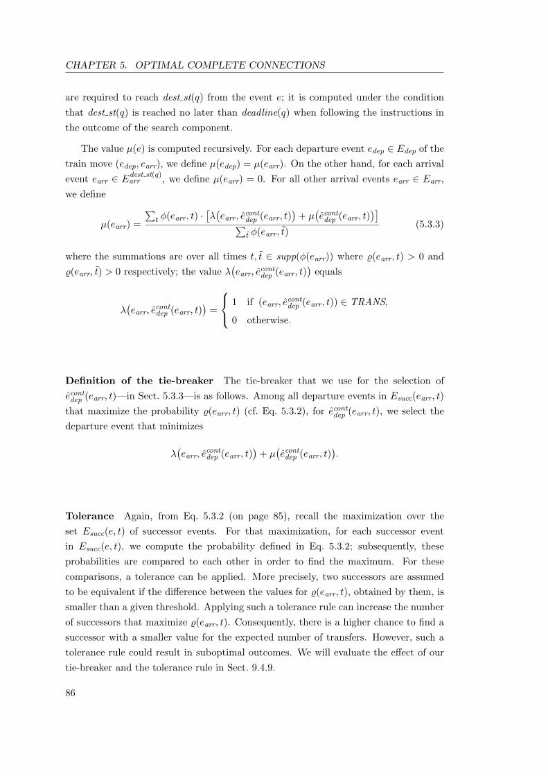
CHAPTER 5. OPTIMAL COMPLETE CONNECTIONS
are required to reach dest st(q) from the event e; it is computed under the condition
that dest st(q) is reached no later than deadline(q) when following the instructions in
the outcome of the search component.
The value µ(e) is computed recursively. For each departure event edep ∈ Edep of the
train move (edep, earr), we define µ(edep) = µ(earr). On the other hand, for each arrival
event earr ∈ Edest st(q)arr , we define µ(earr) = 0. For all other arrival events earr ∈ Earr,
we define
µ(earr) =
∑t φ(earr, t) ·
[λ(earr, e
contdep (earr, t)
)+ µ
(econt
dep (earr, t))]∑
t φ(earr, t)(5.3.3)
where the summations are over all times t, t ∈ supp(φ(earr)) where %(earr, t) > 0 and
%(earr, t) > 0 respectively; the value λ(earr, e
contdep (earr, t)
)equals
λ(earr, e
contdep (earr, t)
)=
1 if (earr, econtdep (earr, t)) ∈ TRANS,
0 otherwise.
Definition of the tie-breaker The tie-breaker that we use for the selection of
econtdep (earr, t)—in Sect. 5.3.3—is as follows. Among all departure events in Esucc(earr, t)
that maximize the probability %(earr, t) (cf. Eq. 5.3.2), for econtdep (earr, t), we select the
departure event that minimizes
λ(earr, e
contdep (earr, t)
)+ µ
(econt
dep (earr, t)).
Tolerance Again, from Eq. 5.3.2 (on page 85), recall the maximization over the
set Esucc(e, t) of successor events. For that maximization, for each successor event
in Esucc(e, t), we compute the probability defined in Eq. 5.3.2; subsequently, these
probabilities are compared to each other in order to find the maximum. For these
comparisons, a tolerance can be applied. More precisely, two successors are assumed
to be equivalent if the difference between the values for %(earr, t), obtained by them, is
smaller than a given threshold. Applying such a tolerance rule can increase the number
of successors that maximize %(earr, t). Consequently, there is a higher chance to find a
successor with a smaller value for the expected number of transfers. However, such a
tolerance rule could result in suboptimal outcomes. We will evaluate the effect of our
tie-breaker and the tolerance rule in Sect. 9.4.9.
86

5.4. COMPUTATION EXTENDED BY TRAVEL TIME OPTIMIZATION
5.4 Computation Extended by Travel Time Optimization
In Sect. 5.3, we presented a recursive function that computes the values %(e, t) and
econtdep (e, t) for an event e ∈ E and a time t ∈ supp(φ(e)). There, we optimized the
expected number of transfers as a secondary criterion. In this section, we extend
the recursive formula from Sect. 5.3 in order to additionally facilitate a travel time
optimization. For the problem variants from Sect. 4.3.3.1–4.3.3.4, this optimization
can be incorporated as a tie-breaker into the computation of the optimal complete
connection—analogously to Sect. 5.3.4. For the problem variant from Sect. 4.3.3.5 (cf.
Minimum Expected Travel Time), this optimization is even the primary criterion for
the computation of the optimal complete connection.
5.4.1 Extension of the Recursive Function
Given a query q, in addition to the probability %(e, t) from Sect. 5.3, we separately
look at every arrival time at the destination. For this, we introduce the probabil-
ity %(e, t, tarr).
Probability %(e, t, tarr) For an event e ∈ E, a time t ∈ supp(φ(e)), and a time
tarr ∈ TIMES where t ≤ tarr ≤ deadline(q), the value %(e, t, tarr) is the probability that
from e the destination station dest st(q) can be reached exactly at the time tarr given
that e takes place at the time t. According to the definition of %(e, t) from Sect. 5.3,
we obtain
%(e, t) =∑
tarr≤deadline(q)
%(e, t, tarr).
Let the set Esucc(e, t) of successor events be defined as in Sect. 5.3.1. The probability
%(e, t, tarr) is described by the following recursive formula.
Recursion anchor For each arrival event earr ∈ Edest st(q)arr at the destination, the
probability %(earr, t, tarr) equals 1 if t ≤ deadline(q) and tarr = t, and 0 otherwise.
Moreover, for each event e ∈ E and times t, tarr ∈ TIMES, the probability %(e, t, tarr)
equals 0 once one of the following conditions is true: t > deadline(q), tarr > deadline(q),
t > tarr, t /∈ supp(φ(e)), or Esucc(e, t) is empty.
For each arrival event earr ∈ Edest st(q)arr at the destination and each t ∈ TIMES, the
value econtdep (earr, t) is set to void. In addition, for each e ∈ E and t ∈ TIMES where
%(e, t) equals 0, the value econtdep (e, t) is set to void.
Recursive step For each event e ∈ E \ Edest st(q), each t ∈ supp(φ(e)), and each
tarr ∈ TIMES where t ≤ tarr ≤ deadline(q), the probability %(e, t, tarr) is defined as
87

CHAPTER 5. OPTIMAL COMPLETE CONNECTIONS
follows. First, we introduce an additional value %(e, t, e, tarr); it is the probability that
from e the destination station dest st(q) can be reached exactly at the time tarr given
that
• the event e takes place at the time t and,
• from e, the journey is continued via e ∈ Esucc(e, t).
Formally, for e ∈ Esucc(e, t), the probability %(e, t, e, tarr) equals
%(e, t, e, tarr) =∑
t∈supp(φ(e))
P (Xe = t∣∣ Xe = t) · %(e, t, tarr). (5.4.1)
The term P (Xe = t∣∣ Xe = t) is defined as in Eq. 5.3.2 (on page 85).
Subsequently, if e is an arrival event, we select the departure event econtdep (e, t) as in
Sect. 5.3.3:
econtdep (e, t) = arg max
{e ∈ Esucc(e, t)
∣∣ ∑tarr∈TIMES
%(e, t, e, tarr)}. (5.4.2)
If the set Esucc(e, t) is empty, the value econtdep (e, t) is set to void.
Finally, if e is an arrival event, we define
%(e, t, tarr) = %(e, t, econtdep (e, t), tarr). (5.4.3)
On the other hand, if e is a departure event, we define
%(e, t, tarr) = %(e, t, e, tarr)
where e is the arrival event of the train move (e, e) starting with the departure event e.
This concludes the extended version of the recursive formula that computes the val-
ues %(e, t) and econtdep (e, t). While both of these values are defined as in Sect. 5.3, the
value %(e, t, tarr) allows us to optimize the travel time as a secondary criterion; this
optimization is detailed in Sect. 5.4.2.
5.4.2 Travel Time Optimization
Set Emaxsucc(e, t) For each event e ∈ E and each time t ∈ supp(φ(e)), we define the
set Emaxsucc(e, t) ⊆ Esucc(e, t) of all successor events that maximize the probability from
Eq. 5.4.2 (on page 88). For the problems from Sect. 4.3.3.1–4.3.3.3, more than one
element of the set Esucc(e, t) may maximize the probability from Eq. 5.4.2. On the
88

5.4. COMPUTATION EXTENDED BY TRAVEL TIME OPTIMIZATION
other hand, for the problem from Sect. 4.3.3.5, we have Emaxsucc(e, t) = Esucc(e, t) since
deadline(q) equals +∞.
Note: The latter statement can be wrong if t is a timestamp on the last day of the
timetable such that the destination can not be reached since the timetable does not
contain trains which can be used at a time equal to or later than t. For the sake of
simplicity, we assume that this case never happens. Practically, a timetable information
system could always load a timetable with a sufficient time period in the future, and
allow queries with values for deadline(q) such that the specified problem does not occur.
Since the set Emaxsucc(e, t) potentially contains more than one element, our recursive
function has degrees of freedom which allow us to optimize certain secondary criteria.
In Sect. 5.3.4, we presented a tie-breaker based on the expected number of transfers;
in this section, we present another tie-breaker by which we optimize the travel time of
complete connections based on the value %(e, t, e, tarr) from Sect. 5.4.1.
Note: We can use a tolerance as introduced in Sect. 5.3.4 in order to build the set
Emaxsucc(e, t).
Minimization of the travel time Our tie-breaker selects from the set Emaxsucc(earr, t)
a successor such that the travel time from earr to dest st(q) is minimized. There, the
travel time is the time difference between the time t and the expected arrival time at
dest st(q). While the expected arrival time at dest st(q) depends on the departure event
that is selected from the set Emaxsucc(e, t), the value t has no influence on this optimization.
Hence, for the minimization of the travel time, it is sufficient to select the departure
event that minimizes the expected arrival time. The latter value is computed as follows.
Expected arrival time at the destination From Sect. 5.4.1 (cf. Recursive step),
recall the definition of %(e, t, e, tarr). Under the assumption that the destination is
reached no later than deadline(q), the expected arrival time at the destination station
equals( ∑tarr∈TIMES
tarr≤deadline(q)
%(e, t, e, tarr) · tarr
)·( ∑
tarr∈TIMEStarr≤deadline(q)
%(e, t, e, tarr))−1
. (5.4.4)
Exact definition of the tie-breaker In order to minimize the travel time as the
secondary criterion, from the set Emaxsucc(e, t), we select for econt
dep (e, t) the successor event
that minimizes the expected arrival time (cf. Eq. 5.4.4).
Alternatively, we can optimize a weighted sum of the travel time and the expected
number of transfers (as introduced in Eq. 5.3.3 on page 86) as a secondary criterion.
89

CHAPTER 5. OPTIMAL COMPLETE CONNECTIONS
More precisely, for each event in Emaxsucc(e, t), we compute a weighted sum; we then com-
pare these weighted sums to each other. Given two successors edep, e′dep ∈ Emax
succ(e, t),
let arr time(edep) and arr time(e′dep) denote their expected arrival times respectively;
moreover, trans(edep) and trans(e′dep) denote their expected number of transfers respec-
tively. To determine whether edep dominates e′dep, we evaluate the constraint
wa · arr time(edep) + wt · trans(edep) <
wa · arr time(e′dep) + wt · trans(e′dep)(5.4.5)
where wa, wt ∈ R are the weights for the expected arrival time and the expected number
of transfers respectively. In our computational study, in Sect. 9.4.9, we evaluate our
extended recursive function with the tie-breaker from this section.
5.5 Properties of Complete Connections
We now discuss properties of complete connections which are relevant for our compu-
tational study in Sect. 9.4. They have already been introduced in Sect. 4.3.2 but the
precise definition can be found in this section. In the following, for a complete connec-
tion c, let einitdep ∈ E
dep st(q)dep denote the initial departure event of c (cf. Sect. 5.1.1).
Probability of success In Sect. 4.3.2, we introduced the probability of success ρ(c)
of a complete connection c. For each complete connection c ∈ Cbest(q), computed by
our search component, we define ρ(c) = ρ(einitdep) (cf. Sect. 5.2.1). The probability ρ(einit
dep)
is computed as explained in Sect. 5.3.2.
Note: A complete connection c ∈ C(q) \ Cbest(q) could have a probability of success
ρ(c) < ρ(einitdep) if it does not contain the best instructions for traveling. We will ad-
dress the computation of the probability of the success of such a complete connection in
Sect. 6.2.2.1.
Scheduled departure time In Sect. 4.3.2, we introduced the scheduled departure
time dep time(c) of a complete connection; we define dep time(c) = sched(einitdep).
Expected number of transfers For a complete connection, the expected number
of transfers equals µ(einitdep); the latter value is defined by the recursive formula from
Eq. 5.3.3 (on page 86). This value is computed under the assumption that dest st(q) is
reached no later than deadline(q).
Expected arrival time The expected arrival time of a complete connection can
be computed using the extended recursive function from Sect. 5.4. For a complete
90

5.6. WALK TRIPS IN COMPLETE CONNECTIONS
connection c, it equals
ρ(einitdep)−1 ·
[ ∑tarr∈TIMES
tarr≤deadline(q)
tarr ·( ∑t∈supp(φ(edep))
φ(einitdep, t) · %(einit
dep, t, tarr))
︸ ︷︷ ︸the probability of arriving at dest st(q) at tarr
]. (5.5.1)
This value is computed under the assumption that dest st(q) is reached no later than
deadline(q).
Expected travel time For a complete connection, this value is the time different
between the expected arrival time at dest st(q) and the scheduled departure time at
dep st(q). This value is computed under the assumption that dest st(q) is reached no
later than deadline(q).
5.6 Walk Trips in Complete Connections
So far, we supported transfers with walk trips (cf. Sect. 1.2) in complete connections—
cf. the definitions of econtdep (e, t) and Esucc(e, t) in Sect. 5.1.2 and 5.3.1 respectively. We
now discuss how to support walk trips at the beginning and at the end of complete
connections.
Note: We do not support complete connections consisting of direct walk trips from
dep st(q) to dest st(q).
Walk trips from the departure station In Sect. 5.1.1, we introduced the initial
departure event of a complete connection; so far, we have assumed that the passenger
leaves the departure station of the query via a train move. Actually, the passenger
could walk from dep st(q) to another station that is connected to dep st(q) via a walk
trip, and continue the journey from there by public transport. We support this case as
follows. Given a query q, first we define the sets
Sdep st(q)walk =
{s ∈ S
∣∣∣ (dep st(q), s)∈WALKS
}and
Ewalkdep =
⋃s ∈ Sdep st(q)
walk
{es
dep ∈ Esdep
∣∣∣ sched(esdep) ≤ deadline(q)
}.
Then, for each esdep ∈ Ewalk
dep , we create an artificial train move (e′dep, e′arr), and add it
to the timetable; this artificial train move is defined as follows:
• e′dep is a departure event at dep st(q),
91

CHAPTER 5. OPTIMAL COMPLETE CONNECTIONS
• sched(e′dep) = sched(esdep)−min dur(dep st(q), s),
• sched(e′arr) = sched(earr) where earr is the arrival event of the train move
(esdep, earr) ∈ TM,
• min dur(e′dep, e′arr) = min dur(es
dep, earr) + min dur(dep st(q), s),
• ∀t ∈ TIMES : φ(e′dep, t) = φ(es
dep, t+ min dur(dep st(q), s)), and
• (esdep, earr), (e′dep, e
′arr), and their respective events are equivalent in the rest of
the attributes.
From then on, these artificial train moves and their events are part of the timetable,
and the corresponding walk trips can be part of the computed complete connections.
They are only used for the computations for the query q, and are removed from the
timetable as soon as the search component is finished with processing q.
Walk trips to the destination station In Sect. 5.3.2 and 5.4.1, the recursion
anchor is at the arrival events at dest st(q); so far, we have assumed that the passenger
arrives at the destination station of the query via a train move. Actually, the passenger
could arrive at a station that is connected to dest st(q) via a walk trip and walk to the
destination station. We support this case as follows. Given a query q, first we define
the sets
Sdest st(q)walk =
{s ∈ S
∣∣∣ (s, dest st(q))∈WALKS
}and
Ewalkarr =
⋃s ∈ Sdest st(q)
walk
{es
arr ∈ Esarr
∣∣∣ sched(esarr) + min dur(s, dest st(q)) ≤
deadline(q)}.
(5.6.1)
Then, for each esarr ∈ Ewalk
dep , we create an artificial train move (e′dep, e′arr), and add it to
the timetable; it is defined as follows:
• e′arr is an arrival event at dest st(q),
• sched(e′dep) = sched(edep) where edep is the departure event of the train move
(edep, esarr) ∈ TM,
• sched(e′arr) = sched(esarr) + min dur(s, dest st(q)),
• min dur(e′dep, e′arr) = min dur(edep, e
sarr) + min dur(s, dest st(q)),
• ∀t ∈ TIMES : φ(e′arr, t) = φ(es
arr, t−min dur(s, dest st(q))), and
92

5.7. TRANSLATION INTO DYNAMIC PROGRAMMING
• (edep, esarr), (e′dep, e
′arr), and their respective events are equivalent in the rest of
the attributes.
From then on, these artificial train moves and their events are part of the timetable,
and the corresponding walk trips can be part of the computed complete connections.
They are only used for the computations for the query q, and are removed from the
timetable as soon as the search component is finished with processing q.
5.7 Translation into Dynamic Programming
In Sect. 5.3 and 5.4, we presented recursive functions that compute the values econtdep (e, t)
and %(e, t) for e ∈ E and t ∈ supp(φ(e)). Each of these recursive functions can be
translated into a dynamic programming approach. The idea of dynamic programming
is that each subproblem is solved once and its solution is available when it is required
(see [CLRS01], Chapter 15, Page 323). According to our problem, by dynamic pro-
gramming, we compute each of the values econtdep (e, t) and %(e, t)—for each event e ∈ E
and each time t ∈ supp(φ(e))—only once, and store the computed values such that they
are available whenever required.
In Sect. 5.7.1, we present our dynamic programming approach to computing the
values econtdep (e, t) and %(e, t). It can be applied to compute optimal outcomes for all
variants of the problem definition from Sect. 4.3.3. Once the dynamic programming
approach is performed, the optimal outcome of the search component can be delivered
as discussed in Sect. 5.2.2.
Exclusively for the problem variant from Sect. 4.3.3.1 (cf. Latest Departure Subject
to Arrival Guarantee), we then extend our dynamic programming approach by early
termination in order to achieve a better performance. This extension is presented in
Sect. 5.7.2.
5.7.1 The Approach
Let %(e, t) and %(e, t) be defined as in Eq. 5.3.2 (on page 85). We perform the compu-
tations from Sect. 5.3 and 5.4 in a specific order such that the following condition is
satisfied.
Condition 5.7.1 For events e ∈ E and e ∈ Esucc(e, t) as well as for t ∈ supp(φ(e))
and t ∈ supp(φ(e)), the value %(e, t) must be computed and be available prior to the
computation of the value %(e, t). This condition also applies to Eq. 5.4.1 (on page 88).
Our dynamic programming approach is presented in Algorithm 5.1. Given a set
Einput ⊆ E, the function process events(Einput) from Algorithm 5.1 computes the values
93

CHAPTER 5. OPTIMAL COMPLETE CONNECTIONS
1 Function process events(Einput)Data: Set Einput ⊆ E; timetable TT; all functions φ(e), e ∈ E; probability
distributions describing random prepared times and random trainmove durations
Result: %(e, t) and econtdep (e, t) for each e ∈ Einput and t ∈ supp(φ(e))
2 Create empty queue;
3 foreach earr ∈ {Einput ∩ Edest st(q)arr } do
4 queue.push(earr);5 end6 while queue is not empty do7 e← queue.pop();
/* Compute the values %(e, t) and econtdep (e, t) */
8 foreach t ∈ supp(φ(e)) do9 if e ∈ Earr then
10 ( %(e, t), econtdep (e, t) )← process arrival(e, t);
11 else /* e ∈ Edep */
12 %(e, t)← process departure(e, t);13 end
14 end/* Add the predecessor events to the queue */
15 foreach (e′, e) ∈ { TM ∪ TRANS ∪ DW } do16 if e′ ∈ Einput then17 queue.push(e′);18 end
19 end
20 end
21 end
Algorithm 5.1: The dynamic programming approach to processing all events ina given set Einput ⊆ E in order to compute the values %(e, t) and econt
dep (e, t) for eachevent e ∈ Einput and each t ∈ supp(φ(e)). The functions process departure andprocess arrival compute the values %(e, t) and econt
dep (e, t) as described in Sect. 5.3
and 5.4; the value econtdep (e, t) is computed only for arrival events.
94

5.7. TRANSLATION INTO DYNAMIC PROGRAMMING
%(e, t) and econtdep (e, t) for each event e ∈ Einput and each time t ∈ supp(φ(e)). In this sec-
tion, the reader may assume that Einput equals E; in Sect. 5.8, we will explain that this
set can be limited to relevant events. The functions process departure(e, t) and pro-
cess arrival(e, t) compute the values %(e, t) and econtdep (e, t) by the recursive formulas from
Sect. 5.3 and 5.4 for departure and arrival events respectively. Each value computed
for some event is subsequently stored so that it is available whenever required.
The queue from Algorithm 5.1 maintains events. It is a dial queue as introduced in
Sect. 3.13.4 with the following difference: the pop operation delivers the events sorted
according to their scheduled event times in descending order; among all events with the
same scheduled event time, departure events are delivered first. The push operation
adds a new element to the queue only if is not already contained in the queue.
Algorithm 5.1 fulfills Condition 5.7.1 (on page 93) as follows. First, for each train
move (e, e) ∈ TM, the event e is processed prior to e since the event e is added to the
queue only after e′ has been processed—cf. Line 15 in Algorithm 5.1. Second, the pop
operation of the queue (described above) ensures that all departure events from the set
Esucc(earr, t) of successor events of an arrival event earr ∈ Earr are visited and processed
prior to earr. The latter statement is based on the following assumption.
Assumption 5.7.1 We assume that the following constellation does not exist in the
timetable; the constellation is illustrated in Fig. 5.2 (on page 96). For an arrival event
es1,tr1arr ∈ Earr and a time t ∈ supp(φ(es1,tr1
arr )), let the set Esucc(es1,tr1arr , t) of successor
events (cf. Sect. 5.3.1) contain the departure events es2,tr2dep and es3,tr3
dep ; it is irrelevant
whether or not s1 = s2 and s1 = s3. Moreover, let es4,tr2arr and es5,tr3
arr denote the arrival
events of the train moves starting with es2,tr2dep and es3,tr3
dep respectively. Algorithm 5.1
could process the event es1,tr1arr prior to one of its both successors if all of the five events—
specified above—have the same scheduled event time. As mentioned, we assume that
this constellation does not exist in the timetable.
This assumption is realistic for real timetables in Germany that we evaluate in our
computational study. For a timetable which violates this assumption, instead of the
approach presented in Algorithm 3.1, we propose to process the nodes in a topological
order (see [CLRS01], Chapter 22, Page 549). A topological ordering exists for the
events in our timetable since the timetable can be represented as a directed acyclic
graph as described in Sect. 2.1.
5.7.2 Early Termination
We now present an improvement of the dynamic programming approach; it can be ap-
plied when solving the problem variant from Sect. 4.3.3.1 (cf. Latest Departure Subject to
Arrival Guarantee). Algorithm 5.1 processes the events sorted by their scheduled event
95

CHAPTER 5. OPTIMAL COMPLETE CONNECTIONS
es1,tr1arr es2,tr2
dep
es3,tr3dep
es4,tr2arr
es5,tr3arr
transfer or dwell
transfer
train move
duration = 0
train move
duration = 0
Figure 5.2: The figure illustrates a constellation of the events in the timetable; all five events areassumed to have the same scheduled event time. This constellation could result in a processing of theevents in a wrong order. For more details, see Assumption 5.7.1 (on page 95).
times in descending order. Consequently, the departure event edep at dep st(q) with a
probability of success ρ(edep) ≥ ρreq(q) that is visited and processed by Algorithm 5.1
first is the initial departure event (cf. Sect. 5.1.1) of the optimal complete connection
for the query q. Thus, as soon as this departure event is found, we can terminate the
algorithm and deliver the optimal complete connection. This early termination could
take place immediately after Line 14 in Algorithm 5.1. In our computational study, in
Sect. 9.4.12, we demonstrate the speedup obtained by this early termination.
5.8 Relevant Events
In Sect. 5.7, we presented our dynamic programming approach to computing the values
%(e, t) and econtdep (e, t) for all events in the set Einput. We could define Einput = E
and compute the outcome for every query by our dynamic programming approach; in
practice, it would be very inefficient. It is even unnecessary to compute the values
%(e, t) and econtdep (e, t) for each event e ∈ E.
Set Erelevant of relevant events For each query, the computations can be restricted
to a subset of the events that we call the set Erelevant ⊆ E of all relevant events.
It contains each event that is relevant for the computation of the outcome for the
query. In other words, the result of the dynamic programming approach is the same
for Einput = E and Einput = Erelevant. As announced in Sect. 5.3.1, we also restrict
the set of successor events to relevant events. More precisely, for e ∈ Erelevant and
t ∈ supp(φ(e)), from the set Esucc(e, t), we remove all events that are not contained
in Erelevant.
Our definition of the set Erelevant implies that %(e, t) = 0 and ρ(e) = 0 for each
e ∈ E \ Erelevant and each t ∈ TIMES. Moreover, the value econtdep (earr, t) is set to void
for each earr ∈ Earr \Erelevant and each t ∈ TIMES—recall that this value is defined for
arrival events solely.
96

5.8. RELEVANT EVENTS
Overview In Sect. 5.8.1, we precisely define when an event is called relevant. In
Sect. 5.8.2, we demonstrate how to discover the set of all relevant events in a pre-
processing step prior to the dynamic programming approach from Sect. 5.7. After-
wards, in Sect. 5.9, we present a very efficient incremental approach that integrates the
discovery of relevant events into the dynamic programming approach from Sect. 5.7,
and incrementally builds the optimal outcome.
From Sect. 4.3.3, recall that we introduced different variants of our problem defini-
tion. While the approach from Sect. 5.8.2 can be employed to solve each of the problem
variants from Sect. 4.3.3.1–4.3.3.5, the incremental approach from Sect. 5.9 is exclu-
sively designed for the problem variant from Sect. 4.3.3.1 (cf. Latest Departure Subject
to Arrival Guarantee). By the incremental approach a significantly better performance
can be obtained as evaluated in Sect. 9.4.12.
5.8.1 Defintion of Relevant Events
Relevant events The relevant events for a query q are defined as follows. We first
introduce two sets of events: Edep st(q)dep ⊆ Edep st(q)
dep and Edest st(q)arr ⊆ Edest st(q)
dep . An event
e ∈ E is called relevant for q if there is a train connection (cf. Sect. 1.2) in the timetable
that connects some departure event in Edep st(q)dep to some arrival event in E
dest st(q)arr via
the event e. In the following, we define the sets Edep st(q)dep and E
dest st(q)arr .
The sets Edep st(q)dep and E
dest st(q)arr We distinguish between the different variants of
our problem definition from Sect. 4.3.3; the sets Edep st(q)dep and E
dest st(q)arr are defined as
follows.
• For “latest departure subject to arrival guarantee” (cf. Sect. 4.3.3.1) and “maxi-
mum probability of success” (cf. Sect. 4.3.3.2), we define
Edep st(q)dep =
{edep ∈ E
dep st(q)dep
∣∣ sched(edep) ≤ deadline(q)}
Edest st(q)arr =
{earr ∈ Edest st(q)
arr
∣∣ sched(earr) ≤ deadline(q)}.
(5.8.1)
• For “on-trip scenario at a station” (cf. Sect. 4.3.3.3), we define
Edep st(q)dep =
{edep ∈ E
dep st(q)dep
∣∣ ontrip time ≤ sched(edep) < deadline(q)}
Edest st(q)arr =
{earr ∈ Edest st(q)
arr
∣∣ ontrip time ≤ sched(earr) < deadline(q)}
(5.8.2)
where ontrip time is as defined in Sect. 4.3.3.3.
97

CHAPTER 5. OPTIMAL COMPLETE CONNECTIONS
• For “on-trip scenario in a train” (cf. Sect. 4.3.3.4), we define
Edep st(q)dep =
{edep
}Edest st(q)
arr ={earr ∈ Edest st(q)
arr
∣∣ sched(edep) ≤ sched(earr) < deadline(q)}
(5.8.3)
where edep is the departure event of the train move where the passenger is located.
• For “minimum expected travel time” (cf. Sect. 4.3.3.5), we define
Edep st(q)dep =
{edep ∈ E
dep st(q)dep
∣∣ sched(edep) ≥ earliest dep time ∧
sched(edep) ≤ latest dep time}
Edest st(q)arr =
{earr ∈ Edest st(q)
arr
∣∣ sched(earr) ≥ earliest dep time} (5.8.4)
where earliest dep time and latest dep time are as defined in Sect. 4.3.3.5.
Note: In Eq. 5.8.1, we ignored arrival events at dest st(q) with sched(earr) > deadline(q)
where there is a time t ≤ deadline(q) such that φ(earr, t) is greater than zero. We
renounced to add such events to Edest st(q)arr since their scheduled arrival times are later
than the deadline, and using them could have an adverse effect on the sense of reliability
from passengers’ point of view. Alternatively, the definition of the set Edest st(q)arr could
be changed to
{earr ∈ Edest st(q)
arr
∣∣ ∃t ∈ supp(φ(earr)), t ≤ deadline(q)}.
This consideration also applies to Eq. 5.8.2 and 5.8.3.
5.8.2 Discover in Pre-Processing
The set Erelevant of relevant events can be discovered in a pre-processing step prior to the
dynamic programming approach from Sect. 5.7. More precisely, to compute the optimal
outcome for a query, we first discover the set Erelevant and then call Algorithm 5.1 with
Einput = Erelevant.
The approach to discovering the set Erelevant ⊆ E is divided in two steps. First, in
a step called backward mark, presented in Algorithm 5.2, we mark all events that are
contained in train connections which end with arrival events in the set Edest st(q)arr . The
set Erelevant is a subset of the set of all events marked.
In a subsequent step called forward mark, presented in Algorithm 5.3, we build the
set Erelevant of all relevant events. For this, we detect all events that are contained in
train connections which start with departure events in Edep st(q)dep and exclusively consist
98

5.8. RELEVANT EVENTS
Data: Timetable TT; set Edest st(q)arr
Result: Set Emarked ⊆ E of marked events1 Emarked ← ∅;2 foreach earr ∈ Edest st(q)
arr do3 backward mark(earr);4 end5 Function backward mark(e ∈ E)6 if e /∈ Emarked then7 Emarked ← Emarked ∪ {e};8 foreach (e′, e) ∈ { TM ∪ TRANS ∪ DW } do9 backward mark(e′);
10 end
11 end
12 end
Algorithm 5.2: The procedure of marking each event which is contained in some
train connection that ends with an arrival event in the set Edest st(q)arr .
Data: Timetable TT; set Edep st(q)dep ; set Emarked ⊆ E of events marked in the
backward mark step.Result: Set Erelevant ⊆ Emarked of all relevant events.
1 Erelevant ← ∅;2 foreach edep ∈ E
dep st(q)dep do
3 forward mark(edep);4 end5 Function forward mark(e ∈ E)6 if e /∈ Erelevant ∧ e ∈ Emarked then7 Erelevant ← Erelevant ∪ {e};8 foreach (e, e′) ∈ { TM ∪ TRANS ∪ DW } do9 forward mark(e′);
10 end
11 end
12 end
Algorithm 5.3: The procedure of the forward mark step. It builds the setErelevant of all relevant events by detecting all events that are contained in train
connections which start with departure events in Edep st(q)dep and exclusively consist
of events that have been marked in the backward mark step.
99

CHAPTER 5. OPTIMAL COMPLETE CONNECTIONS
of events that have been marked in the first step.
After the set of relevant events is discovered, we restrict the expensive
computations—which are required in order to compute the optimal complete
connection—to relevant events solely. This results in a significant improvement of the
performance of the search component. However, the approach to discovering relevant
events that is presented in this section visits a large number of events in the backward
mark step; this is very time-consuming. In Sect. 5.11, we will present heuristics which
can be applied in order to improve the performance of the approach from this section.
In Sect. 5.9, we present a very efficient approach to discovering relevant events that
is designed for the problem from Sect. 4.3.3.1 (cf. Latest Departure Subject to Arrival
Guarantee). The approaches to discovering relevant events are evaluated in Sect. 9.4.12.
Note: For the problem variants from Sect. 4.3.3.4 and 4.3.3.5, it could be more efficient
to switch the order of the forward and backward mark steps.
5.9 Discovering and Processing Incrementally
We developed an efficient approach that incrementally discovers relevant events and
builds the optimal outcome. It terminates as soon as the optimal outcome is built,
and delivers it. The relevant events in the set Erelevant are not discovered in a pre-
processing step as in Sect. 5.8.2. Instead, the procedures of discovering relevant events
and processing events are linked (the latter is performed by the dynamic programming
approach from Sect. 5.7). In Sect. 5.9.1, we present an abstract view on our incremental
approach. Afterwards, in Sect. 5.9.2, we detail the algorithm.
Note: This approach is exclusively designed for the problem from Sect. 4.3.3.1 (cf.
Latest Departure Subject to Arrival Guarantee).
Note: In this section, we explain the approach combined with the method from Sect. 5.3;
however, it could be combined with the extended method from Sect. 5.4 as well.
5.9.1 Abstract View
Our incremental approach to discovering and processing is iterative. For each query q,
we start with an empty set Eincrelevant; at each iteration, a new subset of Erelevant is
discovered and added to Eincrelevant. These newly discovered events are processed by
the dynamic programming approach from Algorithm 5.1 (on page 94). This iterative
procedure is terminated and the optimal outcome is delivered as soon as all events in the
optimal complete connection have been added to Eincrelevant and the complete connection
can be built. The advantage is that it is not necessary to discover all relevant events but
100

5.9. DISCOVERING AND PROCESSING INCREMENTALLY
only a subset of Erelevant that needs be discovered till an early termination is possible.
In the following, we discuss the variant, invariant, and termination criterion of each
iteration. Before that, we introduce the ordered sequence of departure events.
Ordered sequence of departure events Let e1, e2, . . . , en be an ordered sequence
of all departure events from the set Edep st(q)dep ∩ Erelevant (cf. Sect. 5.8) such that the
events in this sequence are sorted by their scheduled departure times in descending
order. Hence, as introduced in Sect. 5.8 (Relevant events), for i = 1, . . . , n, there are
train connections from ei to events in Edest st(q)arr (cf. Sect. 5.8) which exclusively consist
of relevant events in the set Erelevant.
The variant Initially, the set Eincrelevant is empty. For each iteration i = 1, . . . , n, the
variant is as follows:
1. The set Eincrelevant is extended by all events that are not still contained in Einc
relevant
but are contained in train connections—existing in the timetable—which start
with the departure event ei (cf. Ordered sequence of departure events) and end
with events in Edest st(q)arr .
2. The values %(e, t) and econtdep (e, t) are computed for each event e that is inserted to
Eincrelevant in the i-th iteration—and each time t ∈ supp(φ(e)).
The invariant For each iteration i = 1, . . . , n, the invariant is as follows:
1. After i iterations, the set Eincrelevant comprises all events contained in all train
connections—existing in the timetable—which start with the events e1, e2, . . . , ei
(cf. Ordered sequence of departure events) and end with events in Edest st(q)arr .
2. For each event e ∈ Eincrelevant and each time t ∈ supp(φ(e)), the values %(e, t) and
econtdep (e, t) are correctly computed.
Termination criterion For the query q, the incremental approach terminates after
i ≤ n iterations if ρ(ei) ≥ ρreq(q); in words, it terminates if a complete connection
c with ei as the initial departure event (cf. Sect. 5.1.1) is found where c satisfies the
probability of success required by the query q. The complete connection c is feasible and
optimal according to the definitions in Sect. 4.3.2 (also see below). After termination,
c is delivered as the search component’s outcome. In the worst case, the incremental
approach terminates after n iterations if in the timetable there is no complete connection
satisfying ρreq(q). All computations are limited to Eincrelevant as built till termination.
The termination as described above does not compromise optimality since the rel-
evant departure events at dep st(q) are visited and processed in descending order of
101

CHAPTER 5. OPTIMAL COMPLETE CONNECTIONS
their scheduled event times (cf. Ordered sequence of departure events). If the condition
ρ(ei) ≥ ρreq(q) is true, the complete connection with the initial departure event ei op-
timizes the objective function from Eq. 4.3.1 (on page 73, cf. Latest Departure Subject
to Arrival Guarantee).
5.9.2 Detailed View
Up to now, we described the general idea, the variant, the invariant, and the termina-
tion criterion of the iterative approach. In the following, we detail how the approach
discovers new relevant events that are added to Eincrelevant incrementally, and how these
are processed.
The algorithm is presented in Algorithm 5.4 (on page 103). Initially, the set Eincrelevant
is empty. In order to discover relevant events, the algorithm uses a queue (cf. inc queue)
that is equivalent to the queue from Algorithm 5.1; thus, the events are visited in
descending order of their scheduled times. The queue is initialized with all events in
the set Edest st(q)arr . The iterative approach, introduced in Sect. 5.9.1, is then executed.
Each iteration has three phases; in Algorithm 5.4 these phases can be found in Lines 8–
11, Line 12, and Lines 13–15 respectively. In the following, we explain each phase in
detail.
Phase 1 – discover relevant events The goal of the first phase of the i-th iteration
is to discover all events contained in train connections—existing in the timetable—
which end with arrival events in the set Edest st(q)arr and start with the departure event
ei ∈ Edep st(q)dep ∩ Erelevant; the latter is the i-th departure event at dep st(q) from the
ordered sequence of departure events (cf. Sect. 5.9.1). Some of these events could have
already been discovered and marked in prior iterations; thus, at the i-th iteration, we
only seek for the events that are still not marked as relevant but are contained in the
train connections mentioned above. The first phase has two steps; these are partly
similar to the pre-processing approach from Sect. 5.8.2.
The first step is as follows. Recall that the queue is initialized with all events
in Edest st(q)arr . In the i-th iteration, using the queue, we visit and mark the events
which are contained in train connections ending with events in Edest st(q)arr ; these events
are visited in descending order of their scheduled times. This procedure is finished
as soon as a departure event at dep st(q) is found; it is the i-th departure event at
dep st(q) from the ordered sequence of departure events. In Algorithm 5.4, this step is
called inc backward mark ; the respective function extends the set Emarked of marked
events (which grows in each iteration) and returns the mentioned departure event ei ∈E
dep st(q)dep ∩ Erelevant.
In the second step, we subsequently detect all events that are contained in train
102
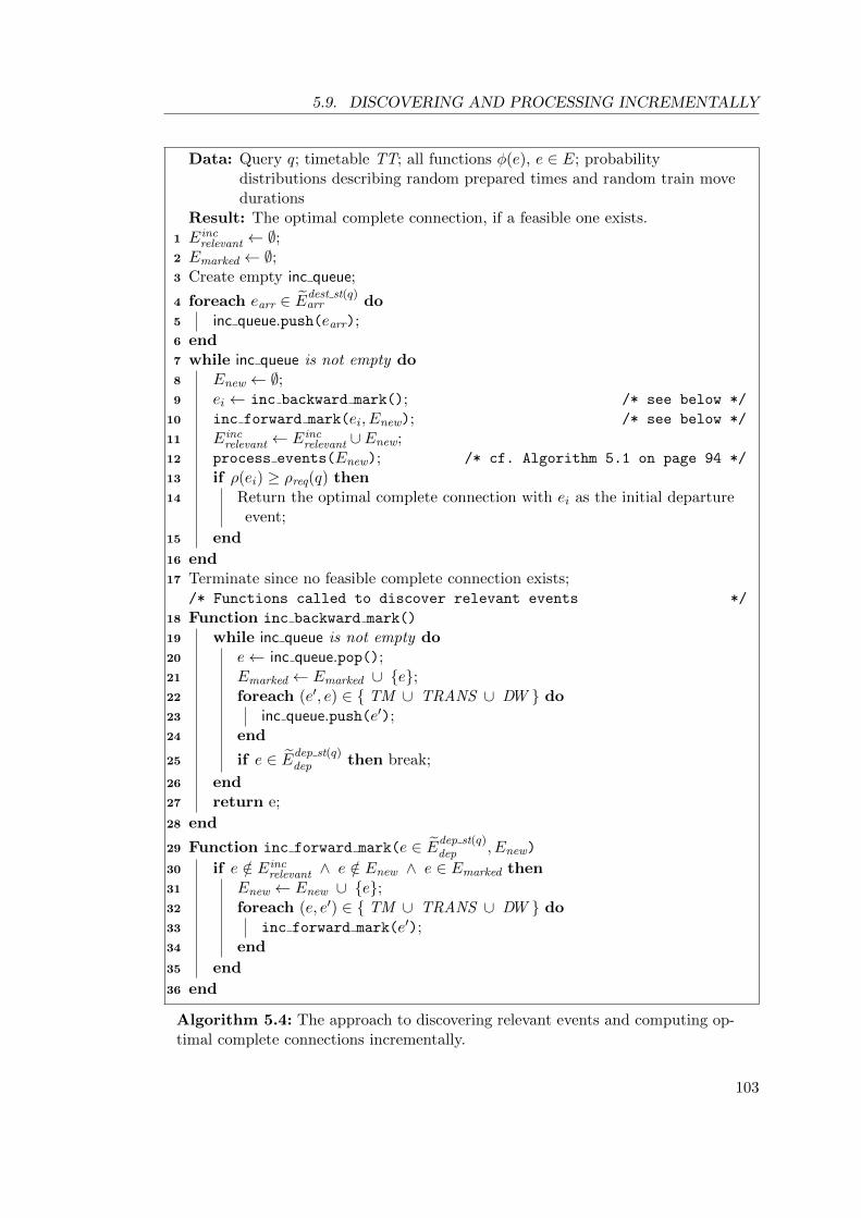
5.9. DISCOVERING AND PROCESSING INCREMENTALLY
Data: Query q; timetable TT; all functions φ(e), e ∈ E; probabilitydistributions describing random prepared times and random train movedurations
Result: The optimal complete connection, if a feasible one exists.1 Einc
relevant ← ∅;2 Emarked ← ∅;3 Create empty inc queue;
4 foreach earr ∈ Edest st(q)arr do
5 inc queue.push(earr);6 end7 while inc queue is not empty do8 Enew ← ∅;9 ei ← inc backward mark(); /* see below */
10 inc forward mark(ei, Enew); /* see below */
11 Eincrelevant ← Einc
relevant ∪ Enew;12 process events(Enew); /* cf. Algorithm 5.1 on page 94 */
13 if ρ(ei) ≥ ρreq(q) then14 Return the optimal complete connection with ei as the initial departure
event;
15 end
16 end17 Terminate since no feasible complete connection exists;
/* Functions called to discover relevant events */
18 Function inc backward mark()
19 while inc queue is not empty do20 e← inc queue.pop();21 Emarked ← Emarked ∪ {e};22 foreach (e′, e) ∈ { TM ∪ TRANS ∪ DW } do23 inc queue.push(e′);24 end
25 if e ∈ Edep st(q)dep then break;
26 end27 return e;
28 end
29 Function inc forward mark(e ∈ Edep st(q)dep , Enew)
30 if e /∈ Eincrelevant ∧ e /∈ Enew ∧ e ∈ Emarked then
31 Enew ← Enew ∪ {e};32 foreach (e, e′) ∈ { TM ∪ TRANS ∪ DW } do33 inc forward mark(e′);34 end
35 end
36 end
Algorithm 5.4: The approach to discovering relevant events and computing op-timal complete connections incrementally.
103

CHAPTER 5. OPTIMAL COMPLETE CONNECTIONS
connections which start with the departure event ei ∈ Edep st(q)dep ∩ Erelevant and exclu-
sively consist of events that have been marked in the first step. All of them are relevant
events; each of them is inserted into the set Enew if it is not already contained in
Eincrelevant. Hence, at the end of the second step of the first phase, the set Enew comprises
all events which have been marked as relevant in the i-th iteration. The set Eincrelevant
is then extended by the events in Enew. In Algorithm 5.4, the second step of the first
phase is called inc forward mark.
Phase 2 – process events As described above, at the end of the first phase of the
i-th iteration, the set Enew comprises all relevant events which have been discovered in
the i-th iteration. For each e ∈ Enew and each time t ∈ supp(φ(e)), the second phase
computes the values %(e, t) and econtdep (e, t)—the latter value for arrival events solely. For
this, the function process events from Algorithm 5.1 is called. However, in contrast to
the approach from Sect. 5.7, all events in the set Eincrelevant \ Enew have already been
processed in prior iterations; for them, the above values need not be computed again
but are persistently available. Thus, the function process events only processes the
events in Enew.
Phase 3 – check the termination criterion The incremental approach is termi-
nated if for the departure event ei ∈ Edep st(q)dep ∩ Erelevant—from the ordered sequence
of departure events—the condition ρ(ei) ≥ ρreq(q) is true. Otherwise, the approach is
continued with the iteration i+ 1.
This concludes the description of our approach to discovering relevant events and com-
puting the optimal complete connection incrementally. The performance of this ap-
proach is evaluated in Sect. 9.4.12.
5.10 Asymptotic Complexity
In this section, we analyze the asymptotic complexity of the search component. Anal-
ogously to Sect. 3.10, the values cm and ca denote the costs of a multiplication and an
addition (or subtraction) of two probabilities respectively. Moreover, we define
nT = maxe∈E|supp(φ(e))| and nD = max
e∈Edep
|Edependarr (edep)|
where the set Edependarr (edep) has been defined in Sect. 3.5.1.1. Last, we define
nS = maxe∈E
t∈supp(φ(e))
|Esucc(edep, t)|.
104

5.10. ASYMPTOTIC COMPLEXITY
Processing a single event An upper bound for the number of multiplications and
additions required for Eq. 5.3.2 (on page 85) is
nT2 · cm
for each arrival event and
nT2 · nS ·
(cm + ca + 2 · nD · (ca + cm)
)for each departure event. For Eq. 5.4.2 (on page 88) of the approach from Sect. 5.4, we
obtain
nT2 · |TIMES| · cm
for each arrival event and
nT2 · nS · |TIMES| ·
(cm + ca + 2 · nD · (ca + cm)
)for each departure event. The summation in Eq. 5.4.2 (on page 88) is over all times in
TIMES; however, in practice, we maintain the information for which values for tarr the
probability %(e, t, e, tarr) is greater than zero. Thus, the summation is actually over a
limited number of values.
In the worst case, for a complete graph, the asymptotic complexity to process an
event is O(|E|2). However, since the values nS , nT , and nD are limited to small values
in practice, an event can be processed in constant time.
Processing a set of events We now discuss the asymptotic complexity of the dy-
namic programming approach from Sect. 5.7 employed in order to process the set Einput
of events. Let ce denote the cost of processing a single event (see above). Let nA be
equal to |TM ∪ TRANS ∪ DW| where each of these sets of activities is limited to
the respective activities between each event pair e, e′ contained in Einput. The cost of
processing the set Einput is
|Einput| · ce + nA · |Einput|
where the second summand is required since the queue performs a duplicate check for
each push operation; we assume a simple duplicate check that iterates over all events
in the queue. In our computational study in Sect. 9.4, we use an implementation that
requires these duplicate checks. Alternatively, we could mark each event that is added
to the queue so that duplicate checks are not necessary anymore. This would improve
the asymptotic complexity of the dynamic programming approach to O(|Einput|+nA).
105

CHAPTER 5. OPTIMAL COMPLETE CONNECTIONS
Discovering relevant events in pre-processing Each of the backward and for-
ward mark procedures from Sect. 5.8.2 has an asymptotic complexity of
O( |E|+ |TM ∪ TRANS ∪ DW | ).
Discovering and processing incrementally We now discuss the asymptotic com-
plexity of Algorithm 5.4 (on page 103). The while-loop (Lines 7–16) will perform a
number of |Edep st(q)dep | iterations in the worst case. Over all iterations, each of the
procedures for forward and backward mark costs
|E|+ |TM ∪ TRANS ∪ DW |.
We assume that the events added to the queue are marked so that duplicate checks are
not necessary anymore.
Over all iterations, the procedure of processing relevant events costs
|Erelevant|+ |TM ∪ TRANS ∪ DW |;
again, each of the latter sets of activities is limited to the respective activities between
each event pair e, e′ contained in Erelevant. For the termination criterion, the probability
ρ(ei) is computed which costs nT · (ca + cm). Altogether, the asymptotic complexity of
Algorithm 5.4 is
O( |Erelevant|+ |TM ∪ TRANS ∪ DW | ).
As we see, compared to the dynamic programming approach from Sect. 5.7 combined
with the approach to discovering relevant events in pre-processing, the incremental ap-
proach from Sect. 5.9 does not reduce the asymptotic complexity. However, in practice,
the incremental approach significantly reduces the number of events which are visited
and processed; the computational study can be found in Sect. 9.4.12.
Note: In our computational study in Sect. 9.4, we use an implementation that requires
duplicate checks.
5.11 Heuristics
In this section, we introduce four heuristics which accelerate the search component but
potentially result in suboptimal outcomes for some queries. All heuristics accelerate
the response times of the search component by decreasing the size of the set of relevant
events (cf. Sect. 5.8). More precisely, for a given query, we remove from the set Erelevant
events that are relevant according to Sect. 5.8.1 but are unlikely to be part of the
106

5.11. HEURISTICS
optimal complete connection for the query.
The heuristic presented in Sect. 5.11.1 can be used for the pre-processing approach
(cf. Sect. 5.8.2) as well as for the incremental approach (cf. Sect. 5.9) to discovering
relevant events. The other heuristics presented in this section are only beneficial for the
pre-processing approach; the incremental approach efficiently delivers optimal outcomes
without the need for them. In Sect. 9.4.11, we will evaluate all heuristics.
5.11.1 Maximum Waiting Time of Passengers
As discussed by [Sch09] (cf. Sect. 10.3.3.2), passengers do not desire long waiting times
at stations. [Sch09] proposes a realistic assumption to limit the maximum waiting time
of passengers at a station for a transfer. Theoretically, this assumption is a heuristic
that potentially results in suboptimality. However, from a practical point of view, this
loss of optimality is negligible as will be discussed in Sect. 9.4.11. We use this realistic
assumption as a heuristic in order to significantly reduce the number of relevant events
as follows.
This heuristic modifies the definition of the set Esucc(earr, t) of successor events from
Sect. 5.3.1. Let tmaxwaiting denote the maximum waiting time of passengers. For earr ∈ Earr
and t ∈ supp(φ(earr)), we remove from the set Esucc(earr, t) each departure event edep
for which the condition
sched(earr) + min dur(earr, edep) + tmaxwaiting < sched(edep) (5.11.1)
is true. The parameter tmaxwaiting is part of the experimental setting and will be defined
in Sect. 9.4.11.
Based on the modification of Esucc(earr, t), we modify the procedures of discovering
relevant events from Sect. 5.8.2 and 5.9. Thus, the for-loops in Algorithm 5.2 on page 99
(Line 8) and Algorithm 5.3 on page 99 (Line 8) are adjusted according to the constraint
from Eq. 5.11.1 (see above). In Algorithm 5.4 this adjustment applies to Lines 22 and 32
respectively.
Note: This heuristic is applicable to all problem variants from Sect. 4.3.3.
5.11.2 Earliest Arrival Time at the Destination
We define an earliest time for the arrival at the destination station. This heuristic
reduces the size of the set Edest st(q)arr from Sect. 5.8.1 and, consequently, the number of
events which are marked as relevant. The earliest arrival time is selected depending on
deadline(q) and is part of our experimental setting in Sect. 9.4.11.
107

CHAPTER 5. OPTIMAL COMPLETE CONNECTIONS
5.11.3 Earliest Departure Time
We define an earliest time for the departure from dep st(q). This heuristic reduces
the size of the set Edep st(q)dep from Sect. 5.8.1 and, consequently, the number of events
which are marked as relevant. The earliest departure time is selected depending on
deadline(q) and an estimation of the duration of the complete connection; the selection
is part of our experimental setting in Sect. 9.4.11.
If this heuristic is applied, the procedure of discovering relevant events is modified
as follows. In Algorithm 5.2 on page 99 (Line 6), we do not mark the event e if sched(e)
is earlier than the earliest departure time; analogously, its predecessors are not visited
anymore. In Algorithm 5.4 (on page 103), the same behavior could be applied to the
function inc backward mark.
5.11.4 Cycles Through the Departure Station
When a transfer breaks during the complete connection, in rare, exotic cases, it may
be preferable to travel back to the departure station and take another train from there.
Forbidding such cycles decreases the number of events which are marked as relevant.
To apply this heuristic, in Algorithm 5.2 on page 99 (Line 8), we do not visit the
predecessors of an event anymore if the event is at dep st(q). Again, in Algorithm 5.4
(on page 103), the same behavior could be applied to the function inc backward mark.
5.12 Parallelization
In his master’s thesis [Glo15], Peter Glockner developed and evaluated approaches to
computing optimal complete connections in parallel. There are two general ideas for a
parallelization. First, for each event e ∈ E and each pair of times t, t′ ∈ TIMES where
t 6= t′, the values %(e, t) and econtdep (e, t′) can be computed separately and in parallel.
Second, events in the timetable can be processed in parallel if the computations do not
depend on each other. In [Glo15], such an parallelization approach is discussed.
Briefly, by a parallelization, the computations can be accelerated. However, the
parallelization is not in the focus of this work, and we refer to [Glo15] for more details.
5.13 Implementation
In this section, we provide details on our implementation of the search component from
Chapter 5. We used the programming language C++.
108

5.13. IMPLEMENTATION
5.13.1 Accessing the Timetable
In our implementation, we used the extended variant of the time-expanded graph model
as introduced in Sect. 3.13.1. When discovering relevant events (cf. Sect. 5.8) and
processing them (cf. Sect. 5.7), we access the predecessors and successors of events in
the timetable as follows—such an access is required for example in Lines 22 and 32 in
Algorithm 5.4 on page 103.
Note: In our implementation, the number of successors and predecessors of arrival
nodes is significantly reduced by applying the heuristic from Sect. 5.11.1 (cf. Maximum
Waiting Time of Passengers).
Successors Each departure node (representing a departure event) has exactly one
successor; namely, the arrival node of its outgoing train edge. From each arrival node
vs,trarr ∈ V s
arr, the succeeding departure node vs,trdep can be reached over the dwell edge
except for the very last arrival node of each train. Moreover, the other successors of
vs,trarr which are nodes of other trains—so that a transfer is required—are reachable over
the change layer; that is, they are reachable either via special-transfer edges or via
leaving, waiting, and entering edges.
Last, there are successors of vs,trarr which are reachable via walk trips (cf. Sect. 1.2,
Transfers with walk trips). In order to find them, we access each station s2 which is
connected to s via a walk trip. We then find each departure node vdep ∈ V s2dep where a
transfer from vs,trarr to vdep is feasible according to the timetable; these are all departure
events with a scheduled event time no earlier than the scheduled event time of vs,trarr plus
the duration of the walk trip from s to s2 (cf. Sect. 1.2, Transfers with walk trips).
Predecessors The predecessors of each event can be accessed analogously to the
successors; the graph need be traversed backwards. In our time-expanded graph, model
this is possible since each node knows its incoming edges.
5.13.2 Relevant Events
In Sect. 5.8 and 5.9, we introduced the sets Erelevant and Eincrelevant of relevant events and
presented approaches to discovering them. In our implementation, we extend the nodes
in the graph model by an additional attribute state that assumes the values unknown,
backward, and relevant ; the values have the following meanings:
• unknown: the node has not yet been visited;
• backward : the node has been visited and marked during the backward mark pro-
cedure; i.e. after performing Algorithm 5.2 (on page 99) or inc backward mark—in
109
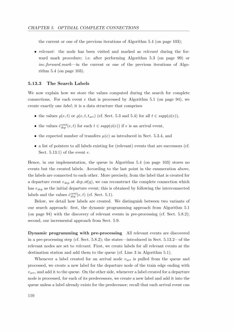
CHAPTER 5. OPTIMAL COMPLETE CONNECTIONS
the current or one of the previous iterations of Algorithm 5.4 (on page 103);
• relevant : the node has been visited and marked as relevant during the for-
ward mark procedure; i.e. after performing Algorithm 5.3 (on page 99) or
inc forward mark—in the current or one of the previous iterations of Algo-
rithm 5.4 (on page 103).
5.13.3 The Search Labels
We now explain how we store the values computed during the search for complete
connections. For each event e that is processed by Algorithm 5.1 (on page 94), we
create exactly one label ; it is a data structure that comprises
• the values %(e, t) or %(e, t, tarr) (cf. Sect. 5.3 and 5.4) for all t ∈ supp(φ(e)),
• the values econtdep (e, t) for each t ∈ supp(φ(e)) if e is an arrival event,
• the expected number of transfers µ(e) as introduced in Sect. 5.3.4, and
• a list of pointers to all labels existing for (relevant) events that are successors (cf.
Sect. 5.13.1) of the event e.
Hence, in our implementation, the queue in Algorithm 5.4 (on page 103) stores no
events but the created labels. According to the last point in the enumeration above,
the labels are connected to each other. More precisely, from the label that is created for
a departure event edep at dep st(q), we can reconstruct the complete connection which
has edep as the initial departure event; this is obtained by following the interconnected
labels and the values econtdep (e, t) (cf. Sect. 5.1).
Below, we detail how labels are created. We distinguish between two variants of
our search approach: first, the dynamic programming approach from Algorithm 5.1
(on page 94) with the discovery of relevant events in pre-processing (cf. Sect. 5.8.2);
second, our incremental approach from Sect. 5.9.
Dynamic programming with pre-processing All relevant events are discovered
in a pre-processing step (cf. Sect. 5.8.2); the states—introduced in Sect. 5.13.2—of the
relevant nodes are set to relevant. First, we create labels for all relevant events at the
destination station and add them to the queue (cf. Line 3 in Algorithm 5.1).
Whenever a label created for an arrival node varr is pulled from the queue and
processed, we create a new label for the departure node of the train edge ending with
varr, and add it to the queue. On the other side, whenever a label created for a departure
node is processed, for each of its predecessors, we create a new label and add it into the
queue unless a label already exists for the predecessor; recall that each arrival event can
110

5.14. CONCLUSION
be the predecessor of multiple departure events. Furthermore, the processed departure
label is added to the list of successor labels of its predecessors’ labels.
Note: If a predecessor is not marked as relevant, we create no label for it.
Incremental approach The set Enew from Algorithm 5.4 (on page 103) is realized
as a C++-vector that contains each node which is marked as relevant in the first
phase of the current iteration. In the second phase, we execute Algorithm 5.1 (on
page 94) with Enew as input. Whenever a departure node is processed, we manage all
of its predecessors which are marked as relevant as explained above for the approach
Dynamic programming with pre-processing. For the other predecessors, no labels are
created but they are stored in a separate data structure (a binary search tree). For
each predecessor, we maintain the list of all its successor labels. At the end of the first
phase of each iteration—where new relevant nodes are discovered, we check each of the
nodes which are stored separately for being discovered as relevant. Finally, for each of
them which has been marked as relevant, we create a label and add it to the queue;
it is then removed from the separate data structure which maintains the predecessors.
An explanation follows.
Above (cf. Dynamic programming with pre-processing), after processing a departure
node, we could completely ignore predecessors that were not marked as relevant—and
create no labels for them—since all relevant nodes had been discovered in the pre-
processing step. In contrast, in each iteration of the incremental approach, a new
subset of the relevant nodes is discovered. Consequently, each departure node vdep that
is processed could have predecessors which are relevant but not discovered yet. On
the one side, at the moment when vdep is processed, we cannot create labels for those
predecessors of vdep since we do not know whether or not they are actually relevant.
On the other side, each label should store pointers to all of its successor labels (see
at the beginning of Sect. 5.13.3). By the separate data structure that maintains such
predecessors, we overcome the problem described.
5.14 Conclusion
In this chapter, we presented our approach to computing optimal complete connections.
For each relevant arrival event and each time in the support of the function describing
its random event time, our search component computes the best departure event to
continue the journey. It delivers a complete connection that guarantees an on-time
arrival; more precisely, the destination is reached no later than the deadline with the
probability of success required in the query. Subject to the on-time arrival guarantee,
the scheduled departure time at the departure station is maximized.
111

CHAPTER 5. OPTIMAL COMPLETE CONNECTIONS
Travel time optimization Our approach optimizes the travel time as a secondary
criterion. On the one side, the scheduled departure time is maximized. On the other
side, when selecting the best departure event to continue the journey, we proceed as
follows. Subject to the probability of success, the continuation is selected that has the
earliest expected arrival time; alternatively, a weighted sum of travel time and number
of transfers is optimized.
Local public transport In Sect. 9.4, we evaluate our optimal approach. We will
see that the approach is efficient for timetables comprising all long- and short-distance
trains in Germany; such a timetable has more than a million departure and arrival
events per day. However, our approach, as introduced in this chapter, is still not suitable
for timetables which include local public transport such as buses and streetcars; such
timetables are by orders of magnitude larger than timetables which comprise short-
and long-distance trains solely. The support for local public transport is left to future
research as will be discussed in Sect. 10.2.
Tickets Transportation companies usually allow passengers to purchase tickets for
specific train rides; the tickets are often limited to specific train categories. For example,
a passenger who has a ticket for a regional train is not allowed to use an intercity
express. In order to facilitate passengers using complete connections as computed by
our approach, transportation companies should accommodate passengers who are faced
by delays. The passengers should be permitted to use other trains in the case of delays.
At least, special tickets should be offered for complete connections. Independently, our
approach could be easily adjusted to find complete connections that comprise trains
of specific categories solely. To realize this, when discovering relevant events, we could
omit all train moves of disallowed train categories.
This concludes our search component. In the next chapter, we will discuss our travel
guidance component.
112

Chapter 6
Travel Guidance
As detailed in Sect. 4.4, we follow a two-stage approach in order to find optimal complete
connections for the problem from Sect. 4.3. The first stage, realized by the search
component (cf. Chapter 5), computes optimal complete connections for queries given.
The second stage is realized by the travel guidance component, which is introduced in
this chapter.
Two main problems Two principal problems overcome by the travel guidance com-
ponent are the following. First, complete connections have a complex structure, and
could contain large numbers of events; therefore, a clear and understandable visualiza-
tion is required. Second, as announced in Sect. 4.3.2, the probability of the success of a
complete connection can be guaranteed only at the time when it is computed. When-
ever the network state has changed due to delays, the probability of the success of a
formerly computed complete connection could be affected. Hence, the main value and
necessity of the travel guidance component is to facilitate access to the instructions
computed by the search component, and to preserve the optimality of the complete
connections delivered.
General idea While traveling, the passenger is guided by the travel guidance compo-
nent. This component interprets the instructions of the outcome of the search compo-
nent. In brief, whenever the passenger waits at a station, the travel guidance component
suggests which train to take next; and whenever the passenger sits in a train, it suggests
what to do at the very next halt: to stay in the train or to leave it. The travel guid-
ance component provides the travelers access to the complete connection (delivered by
the search component). More precisely, it provides access to the values econtdep (e, t) (cf.
Sect. 5.1.2), computed for t ∈ supp(φ(e)) and each event e contained in the complete
connection.
The second problem described above (cf. Two main problems) is solved as follows.
113

CHAPTER 6. TRAVEL GUIDANCE
Whenever a formerly computed complete connection is affected by delays, the travel
guidance component updates it by a re-invocation of the search component. This
update step delivers a complete connection that is optimal according to the current
situation in the train network. Thus, the instructions provided to the traveler are kept
optimal and up to date.
Related work [FMHS08] and [Sch09] presented an approach to the travel guidance
component that checks train connections (as defined in Sect. 1.2) for their feasibility
according to real times (cf. Sect. 1.3.2). It computes alternative continuations for
infeasible train connections. Our approach to preserving the optimality of complete
connections is based on their approach.
Overview We here discuss different possible realizations of the travel guidance com-
ponent. A travel guidance component could solve each of the two above problems to
a greater or lesser extent. In Sect. 6.1, we attend to the first problem; two different
visualizations of complete connections are presented. In Sect. 6.2, the second problem
is addressed. Finally, we conclude this chapter in Sect. 6.3.
Note: In this chapter, we present exemplary realizations of the travel guidance com-
ponent. However, no evaluations of these approaches are presented since the travel
guidance component is a straightforward implementation task rather than a scientific
contribution. Hence, in this work, we discuss different variants of the travel guidance
component only conceptually.
6.1 Interactive Visualization
In this section, we discuss how complete connections could be presented to travelers. We
first demonstrate a web interface as a graphical user interface that provides a detailed
view on complete connections. We then present a mobile application that provides a
compact but clear presentation of complete connections; it is eminently suitable as a
travel guidance component in order to accompany travelers during their journeys.
We want to thank Sebastian Fahnenschreiber, Felix Gundling, Steffen Maus, and
Hannes Wernery who implemented the graphical user interface and the mobile applica-
tion presented in this section.
6.1.1 Web Interface: a Detailed Visualization
We developed a web interface to visualize complete connections; it is illustrated in
Fig. 6.1. It provides a visualization that is based on the illustration of complete con-
114

6.1. INTERACTIVE VISUALIZATION
Figure 6.1: Web interface presenting a complete connection from Munchen Hbf to Langen(Hess)with a transfer at Frankfurt(Main)Hbf. At Frankfurt(Main)Hbf, there are two different alternativecontinuations with scheduled departure times at 13:18 and 13:33 o’clock respectively. The user issuggested to take the first one if he/she arrives at Frankfurt(Main)Hbf with up to 14 minutes delay,and the second one if the delay is larger.
Figure 6.2: A mobile application presenting a complete connection from Hannover Hbf to MunchenDonnersbergerbrucke. There are transfers at Kassel-Wilhelmshohe and Munchen Hbf ; the latter is atransfer with a walk trip to Munchen Hbf(tief). At Kassel-Wilhelmshohe, there are two alternativecontinuations that depart at 12:00 and 12:23 o’clock. By touching the departure times or swiping tothe left or to the right, the user can switch between the available alternative continuations in order togather information about them.
115
CHAPTER 6. TRAVEL GUIDANCE
nections from Fig. 5.1 (on page 79). By rectangles, we represent departure and arrival
events in the complete connection; from each rectangle (titled with the station name),
a set of alternative continuations depart. The user can gather information about each
alternative continuation by moving the mouse over each of them. In Appx. A.2, we
present further screenshots of this web interface.
The web interface provides a global view on a complete connection. For simple
complete connections with a relatively small number of alternative continuations, this
view is clear and understandable. In contrast, for larger complete connections, this
visualization is not suitable; it would be unclear and even confusing. To overcome this
problem, we developed another visualization that is presented below in Sect. 6.1.2.
6.1.2 Mobile Application: a Compact Visualization
We developed a visualization that is eminently suitable for complete connections; it
is illustrated in Fig. 6.2 (on page 115). We integrated it into a mobile application
such that, while traveling, users can access the instructions which are computed by the
search component and available in the complete connection.
The course of the complete connection is visualized top-down along the y-axis. If
there are multiple alternative continuations which can be taken after an arrival event,
their departure times are listed horizontally below the arrival event. The user has the
possibility to click on each departure time or to swipe between them in order to access
each alternative continuation.
Passenger localization In Fig. 6.2, the mobile application does not illustrate the in-
formation which alternative continuation should be taken next. It is possible to extend
the visualization in order to display this information analogously to the visualization
from Sect. 6.1.1: clarifying which alternative continuation is the best choice for each
arrival delay expected. Another solution could be the following: the user enters his/her
position as well as the current delay—in the case he/she is in a train, and the travel
guidance component delivers the best instruction to continue the journey.
Alternatively, a travel guidance component that is informed about the real delay
data—as known so far—of all trains in the complete connection could realize the fol-
lowing behavior. Using the delay data and the events in the complete connection, the
passenger could be localized. Whenever the passenger has reached a station s with
a train tr at a time t, the travel guidance component proposes the departure event
econtdep (es,tr
arr , t) to the passenger. In this way, the passenger is guided by the mobile appli-
cation in every situation that occurs during the journey (see also complete connection
updates in Sect. 6.2.2).
If at some station s a transfer is necessary due to the actual situation in the train
116

6.2. PRESERVING THE OPTIMALITY OF COMPLETE CONNECTIONS
network, the passenger should be forewarned so that he/she is prepared for the transfer.
If we assume that the travel guidance component is informed about the current delay
of the train tr in which the passenger is sitting, few minutes prior to the arrival at
the station s, the travel guidance component could predict the arrival time at s quite
reliably. Based on this prediction, the passenger could be forewarned of the upcoming
transfer. However, the best option to continue the journey can be delivered only after
the real time of es,trarr is definitively known.
Real delay data could be provided to the travel guidance component as to the search
component. The passenger can be localized based on the complete connection and the
current delay data of the trains. The localization could be improved by receiving GPS
data from the smart phone of the passenger.
6.2 Preserving the Optimality of Complete Connections
We now focus on the second problem addressed at the beginning of Chapter 6; preser-
vation of the optimality of complete connections after changes to the train network
due to delays and other real-time incidents (cf. Sect. 1.3). We discuss two different
variants of the travel guidance component; technically, the main difference between the
variants is in the interaction between the search component and the travel guidance
component. In 6.2.1, we present an interaction variant where the search component is
executed once for each query, and the computed complete connection is delivered to
the travel guidance component once. The result is an offline database for the travel
guidance component; the complete connection is computed once and is not updated
anymore. In Sect. 6.2.2, we present a second variant where both components are inter-
connected and exchange data as often as necessary; the result is an online database for
the travel guidance component. Complete connections formerly computed are updated
whenever the network state has changed because of delays and other disruptions. Only
the second one solves the optimality problem introduced at the beginning of Chapter 6.
6.2.1 One-Time Interaction: Offline Database
The database of the travel guidance component could be a complete connection that
is computed once by the search component. In this variant, the travel guidance com-
ponent performs lookups on the computed data, and presents them to the user. The
advantage of this variant is that after the booking stage, the computed complete con-
nection can be stored in the mobile application. Thus, travelers could have detailed
information about their complete connections on their smart phones without any need
for an online Internet connection. If a transfer becomes infeasible because of train de-
lays, the traveler has the possibility to look for other alternative continuations which
117

CHAPTER 6. TRAVEL GUIDANCE
are already computed and available offline in the mobile application.
On the other side, the optimality of the computed complete connections can only be
guaranteed at the booking time. As soon as the network state is changed according to
delays and other disruptions (cf. Sect. 1.3), a complete connection which was optimal
at the booking time could become suboptimal or even infeasible. The probability of
the success of the complete connection could significantly sink, and trains contained
in the complete connection could even be canceled. Hence, the optimality of complete
connections can not be preserved using an offline database. This problem motivated
us for another interaction variant resulting in an online database; it is presented in
Sect. 6.2.2.
6.2.2 Ongoing Interaction: Online Database
We now discuss an ongoing interaction between the search component and the travel
guidance component which results in an online database for the travel guidance com-
ponent. Similar to the variant with an offline database from Sect. 6.2.1, for each query,
the search component computes the optimal complete connection, and delivers it to the
travel guidance component. In contrast to that variant, the interaction between the
both components does not end at this point but the computed complete connection is
updated whenever it is necessary because of changes to the train network (cf. Sect. 1.3).
These updates require ongoing data exchanges between the search and travel guidance
component.
Check and update Trivially, we could recalculate each complete connection for-
merly computed whenever the network state has changed because of delays and other
disruptions. However, for a railway company with millions of travelers per day, this
approach would require very large compute capacities. Thus, we minimize the num-
ber of the expensive recalculations as follows. Whenever the network state changes
after the computation of a complete connection or the last time it was updated, we
check whether the probability of the success of the complete connection is affected by
the delays newly occurred. Only if this is the case, the complete connection needs to
be updated ; more precisely, the complete connection is recalculated. In Sect. 6.2.2.1
and 6.2.2.2, we detail the procedures of checking and updating complete connections.
6.2.2.1 Checking Complete Connections
The check, whether the probability of the success of a complete connection has changed
since its computation or last update, can be triggered manually by the traveler or
automatically by the travel guidance component.
118

6.2. PRESERVING THE OPTIMALITY OF COMPLETE CONNECTIONS
Manual check If a traveler—who has decided for a complete connection—asks the
travel guidance component for the validity of the complete connection, the travel guid-
ance component could ask the search component to recalculate the probability of the
success of the given complete connection as will be explained below (cf. Sect. 6.2.2.1,
Recalculation of the probability of success). The traveler is then informed about how
significantly the probability of success has changed since the computation of the com-
plete connection or its last update. If the probability of success has fallen significantly,
the traveler could manually trigger an update of the complete connection as will be
explained in Sect. 6.2.2.2.
Automatic check A more sophisticated travel guidance component could monitor
all complete connections selected by travelers, check them automatically, and inform
travelers about significant changes. The checks could be performed either in certain
time intervals or whenever a check is actually necessary. While the former can be
simply realized, the latter requires a more complex logic and implementation. More
precisely, for each complete connection c that is monitored and each event e contained
in c, the travel guidance component need be informed about changes to the function
φ(e) (cf. Sect. 3.3). Whenever a function φ(e) has changed for an event e in a complete
connection c, the probability of the success of c has to be recalculated as follows.
Recalculation of the probability of success In Sect. 4.3.2, we introduced the
probability of the success of a complete connection, and we presented a recursive func-
tion to compute this probability in Sect. 5.3. The selection of the best option (cf.
departure event econtdep (e, t)) to continue the journey was integrated into the recursive
function; cf. the maximization in Eq. 5.3.2 (on page 85).
To recalculate the probability of the success of a complete connection c, we can use
the recursive function from Sect. 5.3 with one modification as follows. For every arrival
event earr in the complete connection c, we keep all values for econtdep (earr, t), stored in
c, unmodified; these are the values which have originally been computed by the search
component. More precisely, we assume that the set Esucc(earr, t) of successors (cf.
Sect. 5.3.1) solely comprises the departure event that has originally been selected for
econtdep (earr, t) in the complete connection c. Under this assumption, the value %(e, t) is
then recalculated for each e in the complete connection c and each time t ∈ supp(φ(e)).
After the modification described, the recursive function would not compute the
optimal complete connection but recalculate the probability of the success of the orig-
inally computed complete connection c; this is the probability to reach dest st(q) no
later than deadline(q) when following c.
119

CHAPTER 6. TRAVEL GUIDANCE
6.2.2.2 Updating Complete Connections
If the recalculation of the probability of the success of a complete connection reveals
that this probability has fallen significantly, an update of the complete connection is
required to preserve optimality. This update could be triggered either manually by
the passenger or automatically. For the latter, one could define a threshold for the
minimum change to the probability of success that is required to trigger an update.
Technically, an update is a recalculation of the complete connection. If the traveler
still has not commenced the journey, the search component is reinvoked with the original
query of the traveler. On the other side, if the traveler is already en route, first, a
localization is required, which can be obtained as discussed in Sect. 6.1.2. If he/she
sits in a train, we recompute the complete connection by solving the problem “on-trip
scenario in a train” from Sect. 4.3.3.4. If he/she is waiting at a station, we solve the
problem “on-trip scenario at a station” from Sect. 4.3.3.3.
In such an update procedure, the search component also takes into account new
alternative continuations that were unplanned but are possible due to delays which
change the network state. In a real application, this would make perfect sense. In
Fig. 6.3, by way of example, we demonstrate how a manual update could be triggered
by the traveler. There, the traveler enters his/her position.
6.3 Conclusion
Our search component computes the optimal complete connection for each query q so
that the required probability of success ρreq(q) is met given all information that is avail-
able at the time the search component is executed. The probability of the success of a
complete connection can consequently be guaranteed only at that time. Whenever the
network state has changed, for example due to delays, the probability of the success of
a formerly computed complete connection could be affected. To overcome this prob-
lem, the travel guidance component checks the complete connection and, if necessary,
updates it by a re-invocation of the search component. Moreover, the train guidance
component is responsible for a comprehensive presentation of complete connections to
travelers.
120

6.3. CONCLUSION
Figure 6.3: A mobile application that allows the traveler to update a complete connection manually.First, the traveler clicks on the refresh button; he/she then enters his/her position (left figure) aswell as the current time. Subsequently, the search component is executed and an updated completeconnection is presented (right figure). We can see that the train ICE 1223 is delayed, and the alternativecontinuation departing from Munchen Hbf at 15:08 o’clock is not contained in the updated completeconnection anymore.
121


Chapter 7
Alternative Search Approaches
In Chapter 4, we introduced the problem of finding complete connections which have
a high probability of success. We presented in Chapter 5 an approach that solves this
problem. In this chapter, in Sect. 7.1, we discuss alternative approaches to computing
complete connections. In contrast to the approach from Chapter 5, the approaches from
this chapter are not optimal. However, these are approaches employed by travelers and
state-of-the-art timetable information systems in order to find reliable train connections
or even complete connections. In Sect. 9.4, we evaluate our optimal approach from
Chapter 5 by its comparison to these alternative approaches.
After that, in Sect. 7.2, we present a further approach to the search for reliable train
connection. This approach is based on Pareto Dijkstra (cf. Sect. 2.2) and optimizes the
reliability of train connections as a Pareto criterion.
7.1 On-Time Arrival Guarantee: Alternative Approaches
As already announced, we now discuss alternative approaches to the solution of the
problem specified in Sect. 4.3.3.1 (cf. Latest Departure Subject to Arrival Guarantee).
First, in Sect. 7.1.1, we discuss two approaches used in state-of-the-art timetable in-
formation systems which compute attractive train connections but without regard for
reliability. Then, in Sect. 7.1.2, we discuss an approach that finds train connections
with increased buffer times for transfers and for the arrival prior to the deadline. Last,
in Sect. 7.1.3, we present an alternative approach to computing complete connections.
Note: In Sect. 9.4, we compare our optimal approach from Chapter 5 to each of the
approaches from this section in order to evaluate different properties of the optimal
approach.
123

CHAPTER 7. ALTERNATIVE SEARCH APPROACHES
7.1.1 Disregarding the Probability of Success (DP-L and DP-LP)
In this section, we present two approaches that disregard the probability of success, and
assume that all events take place at their scheduled event times. For each query q, each
of these two approaches delivers a train connection (cf. Sect. 1.2) without alternative
continuations. It is a train connection from dep st(q) to dest st(q) that has a scheduled
arrival time at dest st(q) no later than deadline(q) and satisfies the following condition
respectively:
• For the first approach, denoted by DP-L, the scheduled departure time at
dep st(q) is as late as possible.
• For the second approach, denoted by DP-LP , the train connection is the one
with the latest scheduled departure time at dep st(q) among all Pareto optimal
train connections (cf. Sect. 2.2) that arrive at dest st(q) within the time interval
[deadline(q)− δ, deadline(q)]. The parameter δ will be defined in our computa-
tional study in Sect. 9.4.2. The criteria optimized by the Pareto search are travel
time and number of transfers.
Technically, both approaches are realized by the Pareto Dijkstra algorithm as intro-
duced in Sect. 2.2.2. For both searches, the graph has to be traversed backwards (cf.
Backward search). The first approach is a backward variant of the on-trip search; for
the second approach, an interval for the arrival at dest st(q) is specified.
Probability of success In Sect. 3.7.2, we introduced the probability of the success
of a train connection and presented formulas to compute this value. The probability
of success for train connections computed by the approaches DP-L and DP-LP can be
calculated by the method presented in Sect. 3.7.2.
In Sect. 9.4.6, we will evaluate how often such train connections satisfy the probability
of success ρreq(q) required by the query q.
7.1.2 Minimum Buffer Times for Transfers and Arrival (BT)
From Sect. 1.2, recall that the minimum time required for a transfer activity
(es1,tr1arr , es2,tr2
dep ) ∈ TRANS is denoted as min dur(es1,tr1arr , es2,tr2
dep ). According to the
timetable, the condition
sched(es1,tr1arr ) + min dur(es1,tr1
arr , es2,tr2dep ) ≤ sched(es2,tr2
dep )
is satisfied for each transfer activity. Let us denote the time difference
(sched(es2,tr2
dep )− sched(es1,tr1arr )
)−min dur(es1,tr1
arr , es2,tr2dep )
124

7.1. ON-TIME ARRIVAL GUARANTEE: ALTERNATIVE APPROACHES
as the buffer time of the transfer activity (es1,tr1arr , es2,tr2
dep ). An intuitive approach to
finding reliable train connections is to compute train connections with transfer activities
that satisfy a minimum buffer time.
Note: A similar approach is provided on the official website of the German railway
company [Bah16c]; users can specify a minimum buffer time for the transfers used in
the train connections. That approach is the basis for the approach presented in this
section.
The approach We denote this approach by BT . For each query q, the outcome of
BT is a train connection (without alternative continuations) with a scheduled departure
time at dep st(q) as late as possible such that a minimum buffer time τ is obeyed as
follows:
1. The scheduled arrival time of the train connection at dest st(q) is no later than
deadline(q)− τ , and,
2. for each transfer activity in the train connection, the buffer time (introduced
above) is greater than or equal to τ .
The value τ is a parameter in our experimental setting. In our computational study in
Sect. 9.4.2 and 9.4.7, we will evaluate different values for τ .
Technically, the approach BT is realized by the Pareto Dijkstra algorithm (cf.
Sect. 2.2.2, Backward search) with a modification: during the search for train con-
nections, transfer activities are used only if they obey the minimum buffer time.
Probability of success Analogously to DP-L and DP-LP , the probability of success
of train connections computed by the approach BT can be computed by the method
presented in Sect. 3.7.2.
7.1.3 Connections Extended by Alternatives (CEA)
State-of-the-art traffic information systems do not provide a computation of complete
connections with high probabilities of success. To overcome this problem, some passen-
gers choose an attractive train connection—computed with no regard for the probabil-
ity of success—and change to the next available alternative continuation in case that a
transfer becomes infeasible due to delays.
We developed an approach that, in a sense, simulates the behavior of passengers
who care about alternative continuations as described above. We denote it by CEA.
Analogously to our optimal approach from Chapter 5, the approach CEA computes
complete connections. It aims to compute optimal outcomes; however, it is not optimal
125

CHAPTER 7. ALTERNATIVE SEARCH APPROACHES
for every query. The approach CEA does not compute its outcomes using our recursive
functions from Sect. 5.3–5.4 but it follows another strategy as follows.
The approach CEA consists of three consecutive steps.
1. In the first step, for a query q, the approach CEA computes the set C of all Pareto
optimal train connections (cf. Sect. 2.2) from dep st(q) to dest st(q) that arrive
at dest st(q) within the time interval [deadline(q)− δ, deadline(q)]. The value δ is
a parameter of our experimental setting and will be defined in Sect. 9.4.2. The
criteria optimized by the Pareto search are travel time and number of transfers.
2. In the second step, from each train connection c ∈ C, the approach CEA builds
a complete connection c′ and computes the probability of the success of c′. This
step will be detailed below (cf. Building complete connections).
3. In the third step, among all feasible complete connections built, CEA finally
delivers the complete connection with the latest departure time at dep st(q). From
Sect. 4.3.2, recall that a complete connection c′ is called feasible if ρ(c′) ≥ ρreq(q).
If all complete connections built are infeasible, the outcome of CEA is void.
Building complete connections Given a train connection c, the approach CEA
builds a complete connection c′ as follows. In short, we extend the train connection c
by alternative continuations to the destination station dest st(q) of the query q. The
alternative continuations start at the stations where planned transfers could break. In
the same way, alternative continuations are recursively extended by alternative contin-
uations. A more precise definition of CEA follows.
As introduced in Sect. 1.2, let
(e1dep, e1arr), (e
2dep, e
2arr), . . . , (e
idep, e
iarr), . . . , (e
ndep, e
narr)
denote the ordered sequence of all train moves in the train connection c. We initially
start with an empty complete connection c′. The initial departure event of c′ (cf.
Sect. 5.1.1) is set to the departure event e1dep of c. We then set the instructions to
continue the journey (cf. Sect. 5.1.2) as follows.
• For each arrival event eiarr where (eiarr, ei+1dep ) is a dwell activity, we set the value
econtdep (eiarr, t) to the departure event ei+1
dep for each time t ∈ supp(φ(eiarr)).
• For each arrival event eiarr where (eiarr, ei+1dep ) is a transfer activity, we set the
value econtdep (eiarr, t) to the departure event ei+1
dep for each time t ∈ supp(φ(eiarr)) that
126

7.2. RELIABILITY AS PARETO CRITERION
satisfies the condition
t+ min dur(eiarr, ei+1dep ) ≤ sched(ei+1
dep ) + max wait(eiarr, ei+1dep ). (7.1.1)
This definition conforms to the definition of the set of successor events which is
used in the recursive function of our optimal approach (cf. Sect. 5.3.1).
After the above step, if there is no transfer activity in c, the procedure of building
the complete connection c′ is finished. Otherwise, there could exist arrival events earr
in the complete connection c′ where the value econtdep (earr, t) is yet not defined for some
t ∈ supp(φ(earr)). Thus, we search for alternative continuations that can be used in
such situations as follows.
As long as in c′ there is at least one arrival event earr at some station s ∈ S where
the value econtdep (earr, t) is yet not defined for some t ∈ supp(φ(earr)), we add to c′ an
alternative continuation (cf. Sect. 4.1) from s to dest st(q) that can be taken if earr takes
place at the time t. Let edep denote the very first departure event of this alternative
continuation. We require that the condition from Eq. 7.1.1 is satisfied for earr, edep,
and t. We then set the value econtdep (earr, t
′) to edep for each time t′ ∈ supp(φ(earr)) where
t ≤ t′ ≤(sched(edep) + max wait(earr, edep)
)−min dur(earr, edep).
The alternative continuations are found using on-trip searches as discussed in
Sect. 2.2. Among all possible alternative continuations to dest st(q) that can be taken
if earr takes place at the time t, we choose the one with the earliest arrival time at
dest st(q); by this choice, we simulate the behavior of passengers who after a connec-
tion break try to reach the destination as early as possible.
Probability of success Once a train connection is extended to a complete connection
as described above, the probability of the success of the complete connection can be
computed. Recall that the value econtdep (earr, t) is set for each arrival event earr in the
complete connection and each time t ∈ supp(φ(earr)). We compute the probability of
the success of such a given complete connection as discussed in Sect. 6.2.2.1. The result
is the probability to reach dest st(q) no later than deadline(q) when following the given
complete connection.
7.2 Reliability as Pareto Criterion
Within the scope of the bachelor’s thesis by Marco Plaue [Pla16], we developed a further
approach to the search for reliable train connections. In this section, we conceptually
describe this approach; details can be found in [Pla16]. The approach may be attractive
127

CHAPTER 7. ALTERNATIVE SEARCH APPROACHES
if reliability should be optimized as a criterion beside other criteria such as travel time
and number of transfers. It is based on the Pareto Dijkstra algorithm.
The approach is based on a definition of reliability which is explained in Sect. 7.2.1.
The search algorithm is detailed in Sect. 7.2.2.
7.2.1 Reliability Assessment
The reliability of a train connection is assessed based on the functions φ(earr), earr ∈Earr, describing the random times of the arrival events in the timetable (cf. Sect. 3.3).
For each transfer activity (earr, edep) ∈ TRANS, a value unreliability(earr, edep) is intro-
duced that describes the unreliability of the transfer activity; it is defined as follows:
unreliability(earr, edep) = P (Xearr + min dur(earr, edep) > sched(edep))
=∑
t∈supp(φ(earr))t+min dur(earr,edep)>sched(edep)
φ(earr, t).
The definition of unreliability is then extended to train connections. For a train con-
nection c with k ∈ N0 transfers, let (ejarr, ejdep) ∈ TRANS, j = 1, . . . , k, denote the
transfer activities in c. The unreliability of the train connection c equals
unreliability(c) =∑
j=1,...,k
unreliability(ejarr, ejdep).
Hence, given two train connections c1 and c2 where unreliability(c1) > unreliability(c2),
we assume that c2 is more reliable than c1.
Compared to our reliability assessment method from Sect. 3.7, the method from this
section disregards some factors influencing the reliability (such as the waiting times of
the trains for each other). However, the evaluation of the method demonstrated that it
is still realistic [Pla16]; the greater the unreliability value is, the higher the probability
of a connection break is. The advantage of this method is in its simplicity; compared
to the method from Sect. 3.7, it is faster, and less computations are required.
7.2.2 The Search Algorithm
A query is as defined in Sect. 2.2; the outcome is the set of all Pareto optimal train
connections for the query. An arbitrary set of Pareto criteria can be selected to be
optimized. The search approach is an extension of the Pareto Dijkstra algorithm (cf.
Sect. 2.2.2) applied on a time-dependent graph (cf. Sect. 2.1.2). Compared to the basic
version of Pareto Dijkstra from 2.2, there are three main modifications: unreliability
criterion, adjustment of the domination rules, and expansion of the search space; these
128

7.2. RELIABILITY AS PARETO CRITERION
are detailed in the following.
Unreliability criterion The reliability of the train connections is optimized as an
additional Pareto criterion. More precisely, we minimize the unreliability value intro-
duced in Sect. 7.2.1. Recall that each search label (cf. Sect. 2.2.2, Labels) represents
a train connection from the departure station of the query to the station where the
label is created. Each search label is extended by the unreliability value of the train
connection that is represented by the label. For start labels, this value equals zero. For
labels created during the search, this value is set as follows.
Recall the creation of the labels during the search (cf. Sect. 2.2.2, Creating labels
during the search); given an existing label l at a node v ∈ V and an outgoing edge
(v, w) ∈ A of v, a new label l is created at the node w. Whenever taking the edge (v, w)
requires a new transfer in the train connection, first, the unreliability of this transfer
is assessed by the approach from Sect. 7.2.1. The unreliability value of l is then set to
the unreliability value of l plus the unreliability value of the transfer activity. On the
other hand, if taking (v, w) does not result in a new transfer activity, the unreliability
value of l is set to the unreliability value of l.
Adjustment of the domination rules According to the Pareto dominance rules
from Sect. 2.2.1, a label l cannot dominate another label l′ if the unreliability value of l
is greater than the unreliability value of l′. Additionally, we must adjust the domination
rules as follows in order to find optimal train connections.
Let l and l′ denote two labels created at the same node v ∈ V at a station s ∈ S.
Let the unreliability value of l be lower than or equal to the unreliability value of l′. In
words, according to the transfer activities up to s, the train connection represented by
l is at least as reliable as the train connection represented by l′. Now, let earr and e′arr
denote the arrival events at the station s of each of these train connections respectively.
We forbid l to dominate l′ if
∃ t ∈ TIMES : P (Xearr ≤ t) < P (Xe′arr ≤ t).
The reason is as follows: according to the functions φ(earr) and φ(e′arr), a traveler
taking the train connection represented by l′ could reach the station s earlier. Hence,
a transfer at s after the label l′ could be more reliable compared to the label l.
Expansion of the search space From Sect. 2.1.2 (cf. Routes), recall that the time-
dependent graph model is based on the following assumption for the computation of
attractive train connections: after the arrival at each station, it is sufficient to consider
solely the very next possible departure on each route at that station. This assumption
129

CHAPTER 7. ALTERNATIVE SEARCH APPROACHES
does not hold when the reliability is optimized as a Pareto criterion. While the transfer
into the very next departing train on a route could be highly unreliable, taking the sub-
sequent departure could result in the most reliable train connection. We consequently
must expand the search space as follows.
From Sect. 2.1.2, recall that each route edge represents a set of train moves. Given
a label l at a node v, the Pareto Dijkstra algorithm creates new labels for each outgoing
route edge (v, w); these are successor labels of l. Let earr denote the arrival event at the
station of v of the train connection represented by l. Moreover, for a route edge (v, w),
let e1dep, e2dep, . . . , e
ndep denote the successive departures of the train moves represented
by (v, w).
In the basic variant of Pareto Dijkstra, we create a new label for the very next
departure of the train move represented by (v, w). From the set of departure events
specified above, let eidep denote this very next departure event where i ∈ {1, 2, . . . , n}.If reliability is an additional Pareto criterion, we must create a new label for each of
the departure events eidep, ei+1dep , . . . , e
jdep where ejdep is the earliest departure event such
that
max{t ∈ supp(φ(earr))
}+ min dur(earr, e
jdep) ≤ sched(ejdep).
This concludes the description of the approach; more details can be found in [Pla16].
7.3 Conclusion
In this chapter, we discussed alternative approaches to the search for reliable train
connections and complete connections. The approaches from Sect. 7.1 aim to solve
the problem from Sect. 4.3.3.1 (cf. Latest Departure Subject to Arrival Guarantee). In
our computational study in Sect. 9.4, these approaches are compared to our optimal
approach from Chapter 5.
The approach from Sect. 7.2 is an extension of the Pareto Dijkstra algorithm. It
may be attractive if reliability should be optimized as a criterion beside other criteria
such as travel time and number of transfers. It could be combined with the approach
presented in Sect. 8.3.3 in order to compute reliable intermodal connections.
130

Chapter 8
Reliable Intermodal Connections
In the previous chapters, we addressed the reliability assessment for train connections
and the computation of reliable complete connections. In this chapter, we first extend
our reliability assessment to intermodal connections. As discussed in Sect. 1.4, inter-
modal connections consist of public transport but also of parts where individual modes
of transport are used. More precisely, we focus on individual modes of transport for
which the availability is not guaranteed. Examples include car sharing and bike sharing
services since there is no guarantee they will be available when required. We predict the
availability of cars and bikes by evaluating historical availability data concerning car
and bike sharing stations. This method helps us to assess the reliability of intermodal
connections. We then discuss approaches to searching for reliable intermodal connec-
tions. Our main contribution is the integration of the reliability assessments into the
search for intermodal connections.
After that, we address the problem of connection breaks late at night, particularly
for the case in which a destination cannot be reached prior to the end of operations.
We propose a search approach that finds intermodal connections with taxi rides to the
destination or overnight stays in hotels. Our approach aims to satisfy the passengers
and to minimize the costs for the railway company.
Overview In Sect. 8.1, we discuss the state-of-the-art. Our reliability assessment for
intermodal connections is presented in Sect. 8.2. Then, in Sect. 8.3, we discuss the
search for reliable intermodal connections. Last, in Sect. 8.4, we address the problem
of connection breaks late at night.
Joint contribution The approaches presented in Sect. 8.2 and 8.3 are joint con-
tributions of Felix Gundling and the author of this work. While Felix Gundling is
mainly focused on intermodal train connections, the focus of this work is on reliability
and its integration into the search for intermodal connections. Moreover, we sincerely
131

CHAPTER 8. RELIABLE INTERMODAL CONNECTIONS
thank Sebastian Fahnenschreiber who supported our research on reliable intermodal
connections with helpful hints and suggestions as well as code implementations.
8.1 Related Work
As mentioned in Sect. 1.4, intermodal connections have been addressed by [Gun15,
Gun14, Arn14] in the research group Algorithm Engineering at the Technische Uni-
versitat Darmstadt, Germany. Our research is based on the approaches introduced by
them, and our implementations were extensions of their code base.
To the best of our knowledge, the problems of connection breaks late at night
and finding reliable intermodal connections have not been addressed so far in the lit-
erature. There are various works which focus on the reliability of individual modes
of transport, for example, predictions for the availability of parking spaces [CBM12].
However, reliable intermodal connections—which are a combination of reliable rides in
public transport and reliable rides with individual modes of transport—have not been
considered so far.
8.2 Reliability Assessment
In this section, we present a method of assessing the reliability of intermodal connec-
tions. As discussed in Sect. 1.4, each intermodal connection consists of an initial and
an end part where individual modes of transport are used. In the middle, there is a
train connection as defined in Sect. 1.2. Hence, for this public transport part, we can
assess the reliability exactly as introduced in Sect. 3.7. The reliability assessment for
the initial part and the end part is discussed in the following.
In this work, we assume that individual modes of transport such as walking, indi-
vidual cars, individual bikes, and taxis are reliable. In contrast, for station-based car
and bike sharing (cf. Sect. 2.3.1), there is no guarantee that at the respective station a
car or a bike actually will be available. While passengers desire to plan their journeys
beforehand, the availabilities of car sharing and bike sharing services are usually known
for the current situation solely. There is no guarantee that there will be a car or a bike
that can be used at the time when the passenger arrives at the car sharing or bike
sharing station respectively.
Note: A similar problem occurs when using an individual car and parking spaces close
to train stations have limited capacities. There is no guarantee that the passenger finds
a parking close to the train station. The solution which we propose for car sharing and
bike sharing is also applicable in order to predict the availability of parking areas.
132

8.2. RELIABILITY ASSESSMENT
In the following, for the sake of convenience, we will focus on bike sharing but
the approaches presented here are also applicable to car sharing. First, in Sect. 8.2.1,
we explain how to retrieve predictions for the availabilities of the bikes. Then, in
Sect. 8.2.2, we explain how the reliability of an intermodal connection can be assessed
based on the predictions.
8.2.1 Predictions Based on Historical Data
We predict the availability of an individual mode of transport by evaluating historical
availability data. In this work, we assume that the day of week and the time of day are
two factors influencing the bike availabilities. Given a bike sharing station bst, a day
of week d, and an hour of day h, the prediction for the availability is a number n ∈ N.
In words, we predict that n bikes are available at the station bst on the day of week d
and at the hour of day h.
The predictions are computed as follows. Usually, bike sharing providers have
interfaces which can be used in order to retrieve the current availability state [Arn14].
We gather availability data about the bike sharing stations over a sufficient time period.
By evaluating this data, we compute predictions for the availability of the bikes. In the
following, we elucidate these procedure.
First step: gathering availability data We first need to gather data about the
availabilities of the bikes. For this, we gather availability data by sending requests to
the interfaces of the bike sharing providers periodically; this procedure is repeated over
a sufficient time period (three months by way of example). The response to such a
request usually contains the number of available bikes at each station. Formally, for
each bike sharing station bst of a bike sharing provider, we retrieve a data tuple (bst, t, n)
where bst is the respective bike sharing station, t is time at which the availability is
queried, and n ∈ N is the number of bikes available at bst at the time t.
Second step: classifying gathered data We then classify the gathered data ac-
cording to factors influencing the bike availabilities; we assume that the bike avail-
abilities depend on the day of week and the hour of day. Therefore, we associate the
data tuples (bst, t, n) to new data tuples (bst, d, h) where d ∈ { Mon, Tue, Wed, Thu,
Fri, Sat, Sun } and h ∈ {0, 1, 2, . . . , 23} are the day of week and the hour of the day
respectively. More precisely, each data tuple (bst, t, n) is associated to the data tuple
(bst, d, h) where the point in time t is at the day of week d and at the h-th hour of day.
Third step: predictions After the classification in the second step, for each bike
sharing station bst, each day of week d, and each hour of day h, we have a set of
133
CHAPTER 8. RELIABLE INTERMODAL CONNECTIONS
availability values: the values n from the data tuples (bst, t, n). Let the set N(bst, d, h)
comprise all availability values for bst, day d and hour h. In order to obtain a prediction
for the bike availability at a station bst, on a day d, and at the h-th hour of day, different
aggregators can be applied as follows.
• Average: We can compute the average over all values in N(bst, d, h). By way of
example, we could make a point that between eight o’clock and nine o’clock on
Mondays, there are five bikes on average at bst.
• Minimum: Computing the minimum over all values in N(bst, d, h) would result
in a lower bound for the availability. We believe that this aggregator is too
conservative. As soon as there is one data tuple (bst, t, n) where n equals zero,
the minimum value would be zero.
• Quantile: We could compute various quantiles over the set N(bst, d, h). This
would result in statements such as between eight o’clock and nine o’clock on
Mondays, at bst, four bikes can be found with a 90% guarantee.
Depending on the individual mode of transport and the gathered data, a suitable
aggregator should be selected. One could evaluate different aggregators in order to
find out by which of them realistic predictions can be obtained. This concludes our
method of computing predictions for bike availabilities. In Sect. 8.2.2, we discuss how
the reliability of an intermodal connection can be assessed based on the predictions
from this section.
8.2.2 Reliability Assessment Based on the Predictions
Given an intermodal connection c, we assess the reliability of the initial and the end
part of c based on the predictions from Sect. 8.2.1. From Sect. 1.4 and Fig. 1.4 (on
page 12), recall that, in the station-based bike sharing model, the passenger collects a
bike from a bike sharing station and returns it at another bike sharing station. The
station at which the bike is returned has no influence on the reliability. In contrast,
the availability of a bike at the station where a bike is collected is crucial; thus, the
assessment is derived from the prediction for that station.
First, for the initial part as well as the end part of the intermodal connection c
where bike sharing is used, we retrieve the prediction for the bike sharing station where
a bike is collected. For the predictions from Sect. 8.2.1, we require the day of week and
the hour of day; both can be retrieved from the intermodal connection c (cf. Sect. 1.4,
Intermodal connections).
Based on the predictions, we then assess the reliability of the individual and the
end part of c. We discuss two assessment methods: binary classification and multiclass
134

8.2. RELIABILITY ASSESSMENT
classification; these are as follows.
Binary classification: reliable or unreliable Let bst1 and bst2 denote the bike
sharing stations where the bikes are collected for the initial and the end part of the
intermodal connection c respectively. Moreover, let n1, n2 ∈ N denote the predictions
for the availabilities of bikes at bst1 and bst2 respectively.
We define a threshold τ ∈ N. The initial part of c is classified as reliable if n1 ≥ τ
and as unreliable otherwise. Analogously, the end part of c is classified as reliable if
n2 ≥ τ and as unreliable otherwise.
Multiclass classification We define m ∈ N thresholds τ1, τ2, . . . , τm such that τj <
τj+1 for j = 1, . . . ,m − 1. By these m thresholds, we introduce a classification into
m+ 1 classes; the bike sharing stations associated to the classes 1 and m+ 1 have the
lowest and the highest reliabilities respectively. Let bst1, bst2, n1, and n2 be defined
as above. The bike sharing stations bst1 is associated to a class class ∈ {1, . . . ,m+ 1}where class is determined as follows:
class =
1 if n1 < τ1
k ∈ {2, . . . ,m− 1} if n1 ∈ [τk, τk+1)
m+ 1 if n1 ≥ τm.
The station bst2 is classified analogously.
Discussion While the binary classification is simpler, the multiclass classification
makes possible a differentiated view on the bike availabilities. The binary classifica-
tion could be used if unreliable stations should be identified by a hard boundary (the
threshold τ). The multiclass classification could be used to obtain a multilevel assess-
ment; for example it is suitable if reliability is optimized as a Pareto criterion. In the
next section, we will discuss different approaches to the search for reliable intermodal
connections.
For different modes of individual transport, different thresholds need to be defined.
The thresholds should be adjusted to the respective individual mode of transport.
For example, when assuming that bikes are booked more frequently than cars, a spe-
cific number of available cars could indicate a reliable station while the same number
of available bikes indicates an unreliable station. Generally, we could evaluate the
supply-demand balance at each station in order to obtain more accurate reliability
assessments.
135

CHAPTER 8. RELIABLE INTERMODAL CONNECTIONS
8.3 The Search for Reliable Intermodal Connections
In this section, we discuss different approaches to the search for reliable intermodal
connections and reliable intermodal complete connections. Intermodal connections have
been discussed in Sect. 1.4; intermodal complete connections will be introduced below.
Queries A query q comprises a starting location and a destination location as well as
a time interval [begin(q), end(q)] for the start of the journey from the starting location
(for sake of convenience, we do not discuss the on-trip scenario here). The passenger
seeks for a reliable journey from the starting location to the destination location that
starts in the time interval [begin(q), end(q)].
The search approaches Given a query, we first retrieve the routes for individual
modes of transport; these are denoted as individual routes (cf. Sect. 2.3.1). We then
assess the reliability of each individual route. These two steps (retrieve and assess)
are explained in Sect. 8.3.1; they are the prerequisite for all search approaches that we
discuss here. The search approaches are the following.
1. Finding reliable intermodal connections: From Sect. 7.1.2 and 7.2, recall the
approaches that compute reliable train connections based on Pareto Dijkstra.
We discuss two methods of extending a search approach, such as those from
Sect. 7.1.2 and 7.2, to the computation of reliable intermodal connections:
(a) We solely use rides by individual modes of transport that are classified as re-
liable by the binary classification from Sect. 8.2.2; this approach is discussed
in Sect. 8.3.2.
(b) We use the multiclass classification from Sect. 8.2.2, and optimize the re-
liability of the initial and end part of the intermodal connections as an
additional Pareto criterion; this approach is discussed in Sect. 8.3.3.
2. Finding reliable intermodal complete connections: An intermodal complete con-
nection is a complete connection (cf. Sect. 4.3.2) that is extended by an initial
part as well as end parts where individual transport is used. The initial part con-
nects the starting location to a public transport station at which the journey by
public transport starts. Each of the alternative continuations of the intermodal
complete connection has an end part where individual modes of transport are
used in order to reach the destination location. In Sect. 8.3.4, we propose an
approach to computing reliable intermodal complete connections.
136

8.3. THE SEARCH FOR RELIABLE INTERMODAL CONNECTIONS
For all approaches, we use the time-dependent graph model from Sect. 2.1.2. More-
over, for all approaches, we require the step to retrieve the individual routes and their
reliability assessments; this common step is explained in Sect. 8.3.1.
Note: We implemented the approaches from Sect. 8.3.2 and 8.3.4; sample results can
be found in Appx. A.2. The approach from Sect. 8.3.3 is only discussed conceptually.
In this work, we do not evaluate the approaches to computing reliable intermodal con-
nections and intermodal complete connections.
8.3.1 Retrieving Individual Routes and Their Assessments
As announced, the first step of the search for reliable intermodal connections or com-
plete connections is retrieving individual routes and assessing their reliabilities. The in-
dividual routes are computed and retrieved as described in Sect. 2.3.1. Given a query q,
let IRinit and IRend respectively denote the sets of all individual routes computed for
the initial parts and the end parts of the individual connections for q.
Assessment tuples We assess the reliability of each individual route in IRinit and
IRend by the method from Sect. 8.2.2. For the approaches from Sect. 8.3.2 and 8.3.4,
we apply the binary classification from Sect. 8.2.2. On the other side, for the approach
from Sect. 8.3.3, we apply the multiclass classification from Sect. 8.2.2. The result
is a set of tuples for each individual route where each tuple (t1, t2, a) comprises the
reliability assessment a that is valid from t1 ∈ TIMES to t2 ∈ TIMES. In the following,
we detail the procedure of retrieving these tuples.
Note: As explained in Sect. 8.2, we assume that individual modes of transport such
as walking, individual cars, individual bikes, and taxis are reliable. Hence, for the
individual routes of such modes, an assessment is not necessary.
The assessment procedure From Sect. 8.2.1, recall that the reliability assessments
depend on the day of week and the hour of day. Thus, for each individual route,
the reliability needs to be assessed for each time at which the individual route could
be used in the intermodal connection. Recall that the user provides a time interval
[begin(q), end(q)] for the start of the journey at the starting location. The individual
routes in IRinit are consequently used in the time interval [begin(q), end(q)]. Thus, the
reliabilities of the individual routes in IRinit need to be assessed for the time interval
[begin(q), end(q)].
On the other hand, for the individual routes in IRend, we assess the reliability
of each individual route in IRend for the time interval [begin(q), begin(q) + tmax] where
tmax is chosen sufficiently large; for example, twenty-four hours if we limit the maximum
137

CHAPTER 8. RELIABLE INTERMODAL CONNECTIONS
duration of intermodal connections to twenty-four hours. A smaller time interval cannot
be defined since, prior to the search, the time is unknown at which the individual routes
for the end parts of intermodal connections are used.
Subsequently, the parameters day of week and hour of day are derived from the in-
tervals [begin(q), end(q)] and [begin(q), begin(q)+ tmax] for the individual routes in IRinit
and IRend respectively. These time intervals potentially overlap several hours. Thus,
as described below (cf. Splitting a time interval), we first split each of them into subin-
tervals of one hour length (the very first and the very last subinterval can be shorter).
For each individual route in IRinit, we assess the reliability of the individual route for
each subinterval derived from [begin(q), end(q)]. Analogously, for each individual route
in IRend, we assess the reliability of the individual route for each subinterval derived
from [begin(q), begin(q) + tmax]. Finally, as announced before, for each individual route,
we obtain a set of assessment tuples where each assessment tuple (t1, t2, a) comprises
a reliability assessment a for the time interval [t1, t2].
Splitting a time interval Basically, we split a time interval [tbegin, tend] into n + 2
subintervals [tbegin , t
′begin
),[
t′begin , t′begin + 60min
),[
t′begin + 60min , t′begin + 120min),
. . . ,[t′begin + i · 60min , t′begin + (i+ 1) · 60min
),
. . . ,[t′begin + (n− 1) · 60min , t′begin + n · 60min
),[
t′begin + n · 60min , tend
]where n ∈ N0, i = 0, 1, . . . , n − 1, and the time t′begin is the next full hour after tbegin.
We split the intervals [begin(q), end(q)] and [begin(q), begin(q) + tmax] into subintervals
as described for [tbegin, tend]. The parameters day of week and hour of day—required
for the reliability assessment—are then derived from these subintervals; note that the
length of each subinterval is an hour.
Example: Let t0 denote the midnight of a specific day. We split the time interval
[t0 + 30, t0 + 210] into the subintervals [t0 + 30, t0 + 60), [t0 + 60, t0 + 120), [t0 + 120, t0 +
180), [t0 + 180, t0 + 210].
138
8.3. THE SEARCH FOR RELIABLE INTERMODAL CONNECTIONS
8.3.2 Excluding Unreliable Rides
In this section, we discuss an approach that delivers intermodal connections with reli-
able initial and end parts solely. It can be combined with the approaches from Sect. 7.1.2
and 7.2. The approach consists of three steps.
1. First, as described in Sect. 8.3.1, we retrieve the individual routes and their
assessments tuples. For the search approach presented in this section, the as-
sessment a in each assessment tuple (t1, t2, a) is a binary classification such that
a ∈ {reliable, unreliable}.
2. Second, the individual routes are incorporated into the search for reliable inter-
modal connections as will be explained below (cf. Modeling the initial part and
Modeling the end part). An individual route is used in an intermodal connection
solely in the time intervals in which it is classified as reliable.
3. Finally, we perform the Pareto Dijkstra algorithm (cf. Sect. 2.2) in order to find all
Pareto optimal intermodal connections from the starting location to the destina-
tion location. The intermodal connections computed consist of reliable individual
parts solely.
The first and the third step are self-explaining; we now detail the second step. Individ-
ual routes of individual modes of transport which are assumed to be reliable (such as
taxi, individual car, and individual bike) are incorporated into the search as described
in Sect. 2.3. On the other side, for individual modes as bike sharing and car sharing,
we take into account the reliability assessment as follows. From Fig. 1.4 (on page 12),
recall the structure of a station-based individual route; it consists of a walk, a ride,
and a walk again. In the following, let δw1, δr, and δw2 denote the durations of each of
these sections respectively.
Modeling the initial part As described in Sect. 2.3.3, individual routes for the
initial parts of intermodal connections are modeled by creating respective start labels.
Recall that each individual route for the initial part connects the starting location to
a public transport station. For each individual route ir for the initial part, we create
a new start label for each departure event edep ∈ Edep at the destination station of ir
where
• sched(edep)− (δw1 + δr + δw2) ∈ [begin(q), end(q)] and
• there is an assessment tuple (t1, t2, a) of ir such that a = reliable as well as
sched(edep)− (δr +δw2) ∈ [t1, t2). The latter condition ensures that the individual
mode of transport (as bike sharing or car sharing) is used at the time when it is
classified as reliable.
139
CHAPTER 8. RELIABLE INTERMODAL CONNECTIONS
The new label is associated to the route node that represents edep (cf. Sect. 2.1.2), and
the timestamp of the new label is set to sched(edep). The time cost of the start label is
set to δw1 + δr + δw2.
Modeling the end part As described in Sect. 2.3.2, in the basic approach to the
search for intermodal connections, individual routes for the end parts of intermodal
connections are modeled by individual transport edges. For each query, these edges are
added to the time-dependent graph that represents the timetable; after the query is
processed, they are removed. The individual transport edges connect station nodes to
the destination node; the latter represents the destination location.
In order to search for reliable intermodal connections, we introduce time-dependent
individual transport edges. Analogously to the individual transport edges from
Sect. 2.3.2, a time-dependent individual transport edge connects the public transport
station—at which the individual route starts—to the destination node. We create a
time-dependent individual transport edge for each individual route and each of its as-
sessment tuples (t1, t2, a) where a = reliable. The individual transport edge additionally
stores the time interval [t1, t2). Analogously to route edges (cf. Sect. 2.1.2, Edge costs),
the duration of a time-dependent individual transport edge depends on the time it is
used (cf. Sect. 2.2.1, Creating labels during the search). More precisely, given a time
t ∈ TIMES, the length of an individual route edge equals
length =
+∞ if t+ δw1 ≥ t2δw1 + δr + δw2 if t+ δw1 ∈ [t1, t2)
t1 − t+ δr + δw2 if t+ δw1 < t1
where t is the time at which the individual route edge is used. The time difference
t1 − t includes δw1 as well as the waiting time for an available bike—a bike is assumed
to be available no earlier than t1. The values δw1, δr, and δw2 have been defined at the
beginning of Sect. 8.3.2.
Discussion After Pareto Dijkstra is performed (with the desired criteria), we retrieve
Pareto optimal intermodal connections which use reliable individual routes solely. As
announced before, to obtain reliable train connections for the middle parts of the in-
termodal connections, we could apply approaches as discussed in Sect. 7.1.2 and 7.2.
In the next sections, we discuss further search approaches.
140

8.3. THE SEARCH FOR RELIABLE INTERMODAL CONNECTIONS
8.3.3 Reliability as Pareto Criterion
In this section, we discuss an approach that optimizes the reliability of the initial
and end parts of intermodal connections as an additional Pareto criterion. It can be
combined with the approaches from Sect. 7.1.2 and 7.2. The approach consists of three
steps.
1. First, as described in Sect. 8.3.1, we retrieve the individual routes and their assess-
ments tuples. For the search approach presented in this section, the assessment a
in each assessment tuple (t1, t2, a) is a multiclass classification as described in
Sect. 8.2.2.
2. Second, the individual routes are incorporated into the search for reliable inter-
modal connections as will be explained below (cf. Modeling the initial part and
Modeling the end part).
3. Finally, we perform the Pareto Dijkstra algorithm (cf. Sect. 2.2) to find all Pareto
optimal intermodal connections from the starting location to the destination lo-
cation; the reliability of the initial and end parts is optimized as an additional
Pareto criterion as will be discussed below (cf. Pareto criterion for reliability).
Individual routes of individual modes of transport which are assumed to be reliable (as
taxi, individual car, and individual bike) are incorporated into the search as described
in Sect. 2.3. On the other side, for individual modes as bike sharing and car sharing,
we take into account the reliability assessments as follows. From Fig. 1.4 (on page 12),
recall the structure of a station-based individual route; it consists of a walk, a ride,
and a walk again. In the following, let δw1, δr, and δw2 denote the durations of each of
these sections respectively.
Modeling the initial part As described in Sect. 2.3.3, individual routes for the
initial parts of intermodal connections are modeled by creating respective start labels.
For each reliable individual route ir and each of its assessment tuples (t1, t2, a), we
create a new start label for each departure event edep ∈ Edep at the destination station
of ir where
• sched(edep)− (δw1 + δr + δw2) ∈ [begin(q), end(q)], and
• sched(edep)− (δr + δw2) ∈ [t1, t2).
The new label stores the reliability assessment a from the assessment tuple. It is
associated to the route node that represents edep (cf. Sect. 2.1.2), and the timestamp of
the new label is set to sched(edep). The time cost of the start label is set to δw1+δr+δw2.
141

CHAPTER 8. RELIABLE INTERMODAL CONNECTIONS
Modeling the end part Analogously to the search approach from Sect. 8.3.2 (cf.
Excluding Unreliable Rides), we create time-dependent individual transport edges. We
create such an edge for each individual route and each of its assessment tuples (t1, t2, a).
The edge additionally stores the time interval [t1, t2) as well as the assessment a for
the individual route. The durations of the time-dependent individual transport edges
are defined as in Sect. 8.3.2.
Pareto criterion for reliability We introduce a new Pareto criterion for the Pareto
Dijkstra algorithm (cf. Sect. 2.2); it models the reliability of the rides by individual
modes of transport. From Sect. 8.2.2, recall that, by the multiclass classification, we
assign to each individual route a specific class where the lowest and the highest class
refer to the lowest and highest reliability assessment respectively. We optimize this
reliability class as a Pareto criterion. Consequently, during the search, a label with the
reliability class rc cannot dominate another label with the reliability class rc′ if rc > rc′
(cf. Sect. 2.2.1, Pareto Dominance and Pareto Optimality).
Since each intermodal connection has two parts where individual modes of transport
are used, it has up to two reliability assessments for those parts. Each label could store
either the minimum or the average of these both assessments. Another solution is
to use two Pareto criteria; one for the initial part and one for the end part of the
intermodal connections. However, this would result in a higher number of Pareto
optimal intermodal connections. We explain these different methods by taking the
following example illustrated in Table 8.1 (on page 143); the explanations follow here.
Let A, B, Y , and Z be different rides by individual modes of transport where A
as well as B can be used as initial parts, and Y as well as Z can be used as end
parts of intermodal connections. Let 0 and 10 be the lowest and the highest reliability
classes respectively. The reliability assessments for A, B, Y , and Z are 0, 4, 10, and 4
respectively. We assume that there is only one Pareto optimal train connection—the
middle part of the intermodal connections—that can be combined with A or B as the
initial part and with Y or Z as the end part. This results in four possible intermodal
connections, denoted by AY, AZ, BY, and BZ; these use the initial and end parts as
follows: A and Y , A and Z, B and Y , and B and Z respectively.
If we use the minimum value of the reliability classes in order to find the Pareto
optimal intermodal connections, the assessments for the intermodal connections would
be as follows: AY: 0, AZ: 0, BY: 4, and BZ: 4. The intermodal connections which use
A would be dominated. However, the superiority of Y over Z (10 > 4) has no effect on
the result; BY and BZ are assumed to be equally reliable.
Building the average value would result in the following assessments: AY: 5, AZ: 2,
BY: 7, and BZ: 4. We would correctly identify that BY is the most reliable variant.
142

8.3. THE SEARCH FOR RELIABLE INTERMODAL CONNECTIONS
assessment twoconn initial p. end part min avg criteria
AY 0 10 0 5 0, 10AZ 0 4 0 2 0, 4BY 4 10 4 7 4, 10BZ 4 4 4 4 4, 4
Table 8.1: The table illustrates an example with four intermodal connections. We compare differentvariants modeling the reliability assessments of the individual routes. The values which are illustratedbold refer to the intermodal connections which are Pareto optimal according to the applied variant.“min”: the minimum of the assessments for the initial and the end part is chosen for the Pareto criterionfor reliability.“avg”: the average over the assessments is built.“two criteria”: two separate Pareto criteria are used for the two reliability assessments.
However, AY is assumed to be more reliable than BZ although A has a reliability
assessment of 0. One could construct examples where building the average results in
suboptimal results.
Introducing separate Pareto criteria for the initial and the end part would result
in one Pareto optimal intermodal connection: the connection BY; it dominates AY,
AZ, and BZ. We believe this variant is the most suitable; however, for example, if
the reliability assessments were all the same, all intermodal connections specified above
were Pareto optimal. Thus, this approach can result in higher numbers of Pareto
optimal intermodal connections that appear in the result set.
Discussion After Pareto Dijkstra is performed (with the desired criteria), we retrieve
Pareto optimal intermodal connections where the reliability of the individual routes is
optimized as an additional criterion. As announced before, to obtain reliable train con-
nections for the middle parts of the intermodal connections, we could apply approaches
as discussed in Sect. 7.1.2 and 7.2. In the next section, we discuss an approach to the
search for reliable intermodal complete connections.
8.3.4 Intermodal Connections Extended by Alternatives
At the beginning of Sect. 8.3, we defined intermodal complete connections. In this sec-
tion, we extend the approach connections extended by alternative continuations (CEA)
from Sect. 7.1.3 to intermodal complete connections. In order to retrieve intermodal
complete connections with reliable initial and end parts, we first retrieve all individual
routes and then exclude the unreliable ones as described in Sect. 8.3.2.
More precisely, for each query q, we first compute the set of all Pareto optimal
intermodal connections from dep st(q) to dest st(q) that depart in [begin(q), end(q)]
as described in Sect. 8.3.2. For each of these intermodal connections, we build an
143

CHAPTER 8. RELIABLE INTERMODAL CONNECTIONS
intermodal complete connection as explained in Sect. 7.1.3 (cf. Building complete con-
nections). There, we incorporate into the search for alternative continuations the re-
liable individual routes from public stations to the destination location as described
in Sect. 8.3.2. The result is a set of intermodal complete connections which consist of
reliable rides by individual transport.
Since there is no deadline in the search scenario from this chapter, the probability of
the success of such an intermodal complete connection equals 1. According to the CEA
approach from Sect. 7.1.3, such an intermodal complete connection has an alternative
continuation for every situation that could occur with respect to the probability density
functions describing the random times of the departure and arrival events.
Conclusion This concludes the search for reliable intermodal complete connections.
The search for intermodal complete connections which are optimal according to the
problem from Sect. 4.3 is left to future research; we address this issue in Sect. 10.2.
8.4 Late-Night Connections
In this section, we address an important problem in public transportation. Assume
a passenger takes a train connection but it breaks due to delays or other real-time
incidents. The break is late at night such that the destination cannot be reached by
public transport prior to the end of operations. In such a situation, the passenger has
the following options:
• to wait at some station to bridge the nighttime,
• to travel by special night trains or night buses if available,
• to get a taxi transfer to the destination,
• to stay in a hotel overnight and to travel to the destination at the next day.
For the first two options, the passenger must travel during nighttime; usually, this is
undesired by passengers. For the latter two options, we assume that the transportation
company pays the costs; usually, the transportation companies decide on a case-by-case
basis when taxi transfers or hotel stays are offered to passengers.
Delay compensation Since the original connection is broken, the passenger poten-
tially reaches the destination later than planned. Transportation companies usually
must pay a compensation for the delayed arrival. The amount depends on the delay
and the ticket price of the original, broken train connection. According to the policies
of Deutsche Bahn AG [Bah16b], we assume that a delay compensation is paid even in
cases of taxi transfers and overnight stays at hotels.
144

8.4. LATE-NIGHT CONNECTIONS
Taxi transfers and hotel stays We assume that the transportation provider can
organize taxi transfers to the destination; the passenger is collected at some public
transport station. This station is not necessarily the station where the original train
connection is broken. Instead, the passenger could be suggested to travel to a station
that is closer to the destination by public transport. From there on, the passenger is
brought to the destination by a taxi. This option would result in lower taxi costs.
Moreover, we assume that there are public transport stations close to hotels; the set
of all these stations is provided by the transportation company; we denote this set by
SH ⊂ S. Some transportation companies—which offer hotel stays in case of late-night
connection breaks—have contractual agreements with selected hotels.
Two parameters ensure reasonable hotel stays; earliest check-out time and minimum
stay duration. These parameters can be specified by passengers. The passenger does
not desire to left the hotel too early in the morning; the former parameter models this
constraint. The minimum stay duration is a lower bound for the time the passenger
desires to spend in a hotel if a hotel stay is necessary. This time comprises the sleep
time as well as the time required for check-in and check-out.
General solution: late-night connections We compute a set of late-night con-
nections for the described scenario. A late-night connection models one of the travel
options from the enumeration at the beginning of Sect. 8.4. A late-night connection
always starts at the station where the original train connection of the passenger is bro-
ken; it always ends at the destination station. Since a late-night connection potentially
has a taxi transfer to the destination, it can be intermodal. We believe that a taxi
transfer to the destination is the only reasonable individual mode of transport for the
scenario from this section. Thus, in contrast to intermodal connections as defined in
Sect. 1.4, late-night connections have no initial part where individual transport is used.
Our approach is based on the Pareto Dijkstra algorithm (cf. Sect. 2.2). The Pareto
Dijkstra algorithm is extended by a minimization of the travel time during nighttime
and the costs to be paid by the transportation company. Transportation companies
could use our approach in order to get a proper overview about the available options
to accompany passengers after connection breaks late at night. They would still have
the possibility to decide—on a case-by-case basis—which options are actually offered
to the passengers. In Sect. 9.5, we will evaluate the approach from this section. We
discuss our approach in the rest of this section.
8.4.1 The Search Approach
Queries A query comprises a departure station dep st(q) (the station at which
the original train connection is broken), a destination station dest st(q), and a time
145

CHAPTER 8. RELIABLE INTERMODAL CONNECTIONS
ontrip time(q) for the departure. The latter represents the on-trip scenario since, after
the original train connection is broken, the passenger already waits at a station and
asks for an option to reach the destination. Moreover, the query comprises the ticket
price and the planned arrival time of the original, broken train connection; these are
required to compute the compensation amount according to a delayed arrival at the
destination. Finally, the query contains the minimum stay duration and the earliest
check-out time for hotel stays as described in Sect. 8.4 (cf. Taxi transfers and Hotel
stays).
The approach Given a query q, our approach computes a set of attractive late-night
connections; the search approach consists of four steps.
1. We first retrieve a set of reasonable taxi transfers and their costs as will be
discussed in Sect. 8.4.2 and 8.4.3.
2. We then retrieve the costs for hotel stays as will be discussed in Sect. 8.4.3; as
already announced, we assume that there is a known set of stations at which there
are hotels.
3. We extend the time-dependent graph—which represents the timetable—by ad-
ditional edges that represent hotel stays and taxi transfers; this step will be
discussed in Sect. 8.4.4.
4. We finally apply the Pareto Dijkstra algorithm on the extended graph in order to
retrieve the set of Pareto optimal late-night connections. For the Pareto search, we
introduce additional Pareto criteria to minimize the travel time during nighttime
as well as the costs to be paid by the transportation company.
8.4.2 Retrieving Taxi Transfers
In order to incorporate taxi transfers into the search for late-night connections, we
require a pre-processing step prior to employing the Pareto Dijkstra algorithm. We
retrieve a set of reasonable taxi transfers from public transport stations to the desti-
nation station dest st(q) of the query q. First, we define the set of stations ST ⊂ S
where the passenger could be collected by a taxi. These are stations within a specific
radius around dest st(q). We introduce this limitation in order to limit the taxi costs;
the radius is a parameter, and can be specified by the transportation company. The
definition of the radius also accelerates the search since a large number of stations are
excluded which are not relevant for the current query. Since the number of the stations
in the selected radius could still be large, for faster run times, we restrict the selection
146

8.4. LATE-NIGHT CONNECTIONS
to stations where short-distance and long-distance trains halt; thus, bus and streetcar
stations are excluded from the set ST .
Then, from each station s ∈ ST , we compute a taxi transfer to dest st(q). This
can be accomplished using interfaces of taxi service providers if available. Alterna-
tively, we could use solutions as the Open Source Routing Machine in order to compute
taxi routes [LV11]. The costs for the taxi transfers are retrieved as will be described
in Sect. 8.4.3. The taxi transfers are finally incorporated into the search as will be
explained in Sect. 8.4.4.
Note: If the departure station dep st(q) of the query is within the radius around
dest st(q), a direct taxi transfer from dep st(q) to dest st(q) could be a reasonable option.
Our approach even finds such late-night connections.
8.4.3 The Costs Calculation
Delay compensation As described at the beginning of Sect. 8.4, the transportation
company pays compensations for delayed arrivals of passengers at their destinations.
The amount depends on the delay and the original ticket price. We assume that the
function of computing the delay compensation is provided by the transportation com-
pany.
Hotel stay We assume that the cost for a hotel stay is fixed and known. Alternatively,
it could be retrieved from interfaces of the hotel providers in a pre-processing step.
Taxi transfer For a taxi transfer, we assume that the cost depends on the distance;
in addition there is a base price which is added to the distance dependent price. We
assume that there is either a function to compute the price of a taxi transfer or the
services used to retrieve the taxi transfers also price it.
8.4.4 Modeling Taxi Transfers and Hotel Stays
We extend the time-dependent graph (cf. Sect. 2.1.2)—which represents the timetable—
by hotel and taxi edges as illustrated in Fig. 8.1 (on page 148); these edges model hotel
stays and taxi transfers. Once the hotel stays and the taxi transfers are modeled,
we find the set of attractive late-night connections by applying the Pareto Dijkstra
algorithm as will be explained in Sect. 8.4.5. In the following, we introduce hotel and
taxi edges more precisely.
Hotel edges From Sect. 8.4 (cf. Taxi transfers and Hotel stays), recall that at each
station in the set SH ⊂ S there is hotel. For each station s ∈ SH , we introduce a
147

CHAPTER 8. RELIABLE INTERMODAL CONNECTIONS
S
R
R
R
S
R
R
taxi
SR taxi
SR R
hotel
Figure 8.1: The figure illustrates, schematically, sequences of edges and nodes which build late-nightconnections. The dashed ellipses illustrate stations; all nodes in such an ellipse belong to the samestation. The stations at the left and at the right of the figure are dep st(q) and dest st(q) respectively.Station nodes and route nodes are labeled with S and R respectively. Each dashed arrow representsa sequence of edges in the graph—for example a sequence of train moves and transfer activities. Fourdifferent late-night connections are depicted. The first one contains a hotel stay, the second one is adirect taxi transfer, the third one contains a taxi transfer after moving by public transport, and thefourth one solely consists of public transport—for example a special night train.
hotel edge. This edge is a loop, and connects the station node of s to itself.
Analogously to a route edge (cf. Sect. 2.1.2), a hotel edge is time-dependent; its
length depends on the time t ∈ TIMES when the edge is asked for its length by the
Pareto Dijkstra algorithm (cf. Sect. 2.2.1, Create labels during the search). Moreover,
the length depends on the parameters minimum stay duration and earliest check-out
time (cf. Sect. 8.4, Taxi transfers and Hotel stays). Given a time t ∈ TIMES, a
minimum stay duration min stay ∈ N (in minutes), and an earliest checkout time
checkout ∈ TIMES, the length of a hotel edge equals
max{
checkout− t, min stay}.
The price of a hotel edge is a fixed value as described in Sect. 8.4.3. The transfer cost
of a hotel edge equals 0.
Taxi edges In Sect. 8.4.2, we described the computation of the taxi transfers for a
query. Each taxi transfer starts at some station s ∈ ST and ends at the destination
station dest st(q). Each taxi transfer is modeled by a taxi edge that connects the station
node of s to the station node of dest st(q). The length and the price of a taxi edge are
fixed values; they are computed as described in Sect. 8.4.2 and 8.4.3. The transfer cost
for taxi edges equals 0 except for direct taxi edges from the station node of dep st(q)
to the station node of dest st(q); an explanation follows.
148

8.4. LATE-NIGHT CONNECTIONS
From Sect. 2.1.2 (cf. Edge costs), recall that, in the time-dependent graph model,
the edge from a route node to a station node has a transfer cost of 1. For each train
connection, we even count a transfer when taking the edge from a route node at the
destination station to the station node at the destination station. Consequently, each
label at the destination node has a transfer count that is larger by 1 compared to the
correct number of transfers. The Pareto Dijkstra algorithm, as described in Sect. 2.2,
still delivers correct results since the additional transfer is counted equally for all train
connections. In order to compute correct results after adding taxi edges to the graph,
if a direct taxi edge from the station node of dep st(q) to the station node of dest st(q)
is added to the graph, we set its transfer cost to 1 (cf. Fig. 8.1).
8.4.5 The Pareto Search for Late-Night Connections
In order to compute attractive late-night connections, we apply the Pareto Dijkstra
algorithm (cf. Sect. 2.2) on a time-dependent graph that models the timetable and is
extended as described in Sect. 8.4.4. Since we have an on-trip scenario, we exactly
create one start label at the station node of dep st(q) as described in Sect. 2.2.2 (cf.
Creating start labels). The station node of dest st(q) is specified as the destination node
for the search.
Note: If desired, the approach from this section can be combined with the approaches
from Sect. 7.1.2, 7.1.3, and 7.2 in order to find reliable connections. However, for sake
of convenience, we do not consider reliability in this section.
We use the criteria travel time and number of transfers in order to find attractive
train connections. In order to minimize the travel time during nighttime as well as
the costs to be paid by the transportation company (as described at the beginning of
Sect. 8.4), we introduce two additional Pareto criteria denoted as the tp-costs criterion
and the nighttime criterion respectively. These are defined below (cf. The tp-costs
criterion and The nighttime criterion). We will see that an extension of the labels is
required as will be discussed below (cf. The hotel flag). We also discuss an adjustment
of the domination rules during the search (cf. Adjusted domination rules).
The tp-costs criterion This criterion stores the costs to be paid by the transporta-
tion company; this Pareto criterion is minimized during the search. As described in
Sect. 8.4.3, costs are caused in case of taxi transfers or hotel stays. Moreover, the
transportation company must pay compensations in case of delayed arrivals at the des-
tination. The cost criterion for the start label equals zero. During the search, it is
computed as follows. Recall the creation of the labels during the search (cf. Sect. 2.2.2,
Creating labels during the search); given an existing label l at a node v ∈ V and an
149

CHAPTER 8. RELIABLE INTERMODAL CONNECTIONS
outgoing edge (v, w) ∈ A of v, a new label l is created at the node w. The cost criterion
for the label l equals
tp cost(l) = tp cost(l) + tp cost(v, w).
The value tp cost(v, w) denotes the cost caused by taking the edge (v, w); it equals the
delay compensation amount—incurred when taking (v, w)—plus
• the price for the hotel stay if (v, w) is a hotel edge,
• the price for the taxi transfer if (v, w) is a taxi edge, and
• zero otherwise.
As announced in Sect. 8.4.3, we assume that the function of computing the delay
compensation is provided by the transportation company; see Sect. 9.5.1 (cf. Model
and parameters) for an example.
The nighttime criterion This criterion stores the travel time during nighttime; it
is denoted by night travel time. The nighttime is defined as a time interval; for example
from midnight to 5:00 o’clock. This criterion is minimized as a Pareto criterion since
traveling during nighttime is not desired by passengers. For the start label, it equals
zero. Recall the creation of the labels during the search (cf. Sect. 2.2.2, Creating labels
during the search); given an existing label l at a node v ∈ V and an outgoing edge
(v, w) ∈ A of v, a new label l is created at the node w. The nighttime criterion for the
label l equals
night travel time(l) = night travel time(l) + night travel time(t(l), len
)where
• t(l) ∈ TIMES denotes the timestamp (cf. Sect. 2.2.2, Labels) of the label l,
• len denotes the length of the edge (v, w), and
• the function night travel time(t(l), len
)delivers
– zero if (v, w) is a hotel edge and
– the overlap time between the time interval [t(l), t(l) + len] and the nighttime
for all other edge types.
150

8.5. CONCLUSION
The hotel flag We assume that, after a hotel stay, the passenger travels by public
transport to the destination; the transportation company does not pay for a hotel stay
as well as a taxi transfer. Hence, we do not compute late-night connections which
contain a hotel stay as well as a taxi transfer. This constraint is modeled as follows.
Each label for the Pareto Dijkstra search (cf. Sect. 2.2.2, Labels) is extended by a
hotel flag ∈ {0, 1}. For the start label, it is set to 0. Recall the creation of the labels
during the search (cf. Sect. 2.2.2, Creating labels during the search); given an existing
label l at a node v ∈ V and an outgoing edge (v, w) ∈ A of v, a new label l is created
at the node w. The hotel flag for label l equals
hotel flag(l) = hotel flag(l) + is hotel edge(v, w)
where is hotel edge(v, w) delivers 1 if (v, w) is a hotel edge, and 0 otherwise.
We forbid a taxi transfer after a hotel stay as well as multiple hotel stays as follows.
Let l, l, and (v, w) be defined as above. If (v, w) is a taxi or a hotel edge, we create the
label l as the successor of l only if hotel flag(l) equals zero.
Adjusted domination rules We adjust the domination rules (cf. Sect. 2.2.2, Label
dominance) for the comparison of labels at each node except for the destination node.
A label l is not allowed to dominate another label l′ if hotel flag(l) 6= hotel flag(l′). This
constraint ensures that no Pareto optimal late-night connection is dominated during
the search. More explanations follow.
If hotel flag(l) equals 1, the label l cannot use a taxi anymore. In contrast, the label
l′ could still use a taxi if hotel flag(l′) equals 0. Hence, compared to l, the label l′ has
more options for the continuation of the journey. In this case, we forbid a domination
of l′ by l.
On the other side, if hotel flag(l) equals 0 and hotel flag(l′) equals 1, in contrast to l,
the label l′ has already bridged the nighttime. Hence, connections which are constructed
from the label l potentially require longer travel times during the nighttime compared
to connections which are constructed from the label l′. Therefore, in this case, we forbid
a domination of l′ by l.
This concludes the extension of the Pareto Dijkstra algorithm that is required to find
late-night connections. An evaluation of this approach can be found in Sect. 9.5.
8.5 Conclusion
Reliable intermodal connections We discussed a method of assessing the relia-
bility of rides by individual modes of transport. Our method is based on predictions
151

CHAPTER 8. RELIABLE INTERMODAL CONNECTIONS
which are computed using real, historical data. However, instead of our assessment
method, even other assessment methods could be combined with our approaches to the
search for reliable intermodal connections and complete connections. We discussed four
different approaches to computing reliable train connections and complete connections.
The search for optimal complete connections is left to future research.
We have implemented and tested the approaches from Sect. 8.3.2 and 8.3.4. How-
ever, in this work, we do not evaluate these approaches, not least because of the lack
of data for bike sharing and car sharing services.
Late-night connections Train connections could break late at night such that the
destination cannot be reached by public transport prior to the end of operations. We
presented a solution that finds attractive late-night connections for this scenario. We
apply the Pareto Dijkstra algorithm extended by additional criteria minimizing the
travel time during nighttime and the costs to be paid by the transportation company.
This approach is evaluated in Sect. 9.5.
152
Chapter 9
Computational Study
In this chapter, we present evaluations of approaches discussed in this work. We im-
plemented the approaches as extensions of the existing timetable information system
MOTIS (Multi-Objective Traffic Information System); it has been developed in the in-
stitute of Algorithm Engineering at the Technische Universitat Darmstadt in Germany
[Alg16]. The code is written in C++.
We first explain in Sect. 9.1 which data we used for our evaluations. We then
present in Sect. 9.2 evaluations of computations of probability distributions describing
the random times of events in the timetable. In Sect. 9.3, we evaluate the quality of
our reliability assessments from Chapter 3. In Sect. 9.4, we demonstrate an extensive
evaluation of our optimal approach from Chapter 5; the optimal approach is compared
to the approaches from Sect. 7.1. We finally present in Sect. 9.5 an evaluation of the
approach from Sect. 8.4 that computes late-night connections.
9.1 Setup Data
In this section, we explain on which data our evaluations are based.
Timetable We used real timetable data provided to us by the German railway com-
pany, Deutsche Bahn AG [Bah16c]. In addition, they provided to us the values for
minimum dwell and transfer times as well as maximum waiting times (cf. Sect. 1.1
and 1.2). We used timetables with validity periods in the past; the real times (cf.
Sect. 1.3) of a large portion of the events in the timetables have been provided to us
by Deutsche Bahn AG as well.
Functions describing random prepared times From Sect. 3.3.2, recall that, for
each departure event edep ∈ Edep, there is a random prepared time with the probability
153

CHAPTER 9. COMPUTATIONAL STUDY
density function ξ(edep). We collected data about these functions from different sources
as follows.
In our input data, provided by Deutsche Bahn AG, the function ξ(edep) is given
for the very first departure events of the short-distance and long-distance trains of
relevant and frequent train categories. We used the functions for short-distance trains
(S-Bahn) also for streetcars. For the very first departure events of buses, we learned
the respective functions as described in Sect. 3.4.1; for this learning procedure, we
used a history of real delay data kindly provided to us by the local public-transport
organization DADINA [DAD16]. For the rest of the departure events, we simply defined
the following function:
ξ(edep, t) =
1 if t = sched(edep),
0 otherwise.
Functions describing random train move durations From Sect. 3.3.2, recall that
there is a probability density function θ(tm, tdep) for the random duration of each train
move tm ∈ TM and for each possible departure time tdep ∈ TIMES of the departure
event of tm. We collected data about these functions from different sources as follows.
For relevant and frequent classes of short-distance and long-distance trains,
Deutsche Bahn AG provided to us probability density functions for the random dura-
tions of their train moves. We used the functions for short-distance trains (S-Bahn) also
for streetcars. For buses, we learned the respective functions as described in Sect. 3.4.2;
for this learning procedure, we used a history of real delay data kindly provided to us
by the local public-transport organization DADINA [DAD16].
For train moves of the remaining train moves (which are not covered above), we
proceeded as follows. For the evaluations in Sect. 9.2 and 9.3, we generated one-point
probability distributions with a probability of one for the stochastic event that the
real duration of the train move equals its scheduled duration. For the evaluations in
Sect. 9.4, we generated realistic distributions as discussed in Sect. 3.4.3: for the random
duration of such a train move (edep, earr) and for each time tdep ∈ supp(φ(edep)), we
assumed a Cauchy distribution parameterized depending on tdep and the scheduled du-
ration of (edep, earr); the parameters were chosen such that the generated distributions
were realistic; see Appx. A.3 for examples.
Hardware Our computations were carried out on a desktop PC with Intel Xeon CPU
E3-1270v2 3.50GHz and 32 GB of RAM.
154
9.2. DISTRIBUTIONS FOR RANDOM EVENT TIMES
9.2 Distributions for Random Event Times
In Sect. 9.2.1, we present the evaluations of the procedures of computing probability
density functions for random event times. In Sect. 9.2.2, we evaluate the procedure of
updating precomputed functions according to real event times.
9.2.1 Computing the Probability Density Functions
In this section, we evaluate the procedure of computing the probability density functions
describing the random times of events. We evaluate two variants which are as follows:
1. The pre-processing procedure as discussed in Sect. 3.8.2 using the extended ver-
sion of the time-expanded graph from Sect. 3.13.1.
2. The hybrid processing procedure from Sect. 3.8.3 using the time-dependent graph
from Sect. 2.1.2 combined with the dependency graph from Sect. 3.13.2.
Setup Using real timetable data from German railways, we prepared a time-expanded
and a time-dependent graph for the first and the second variant respectively. With the
time-expanded graph, we only modeled long-distance and short-distance trains. With
the time-dependent graph, we additionally modeled local public transport such as buses
and streetcars. We performed the evaluation for the following two days periods in
November 2016: 21-22, 22-23, 23-24, 24-25, 25-26, 26-27, and 27-28; the very first day
was a Monday.
Note: A two days period allowed us to search for train connections that start and end
at the same day as well as train connections that end at the very next day.
Negligible probabilities As explained in Sect. 3.13.3, we dropped negligible prob-
abilities; the parameter ε from that section is set to 10−5 in our computational study.
The cardinality of supp(φ(e)), for each event processed in the evaluation from this
section, never exceeded 135 minutes.
Results The evaluation results are presented in Tables 9.1 and 9.2; the tables give
reports on the number of the events for which we computed the probability density
functions; the run time required for each procedure is listed as well. The number of
all events in Table 9.2 is significantly higher than the number of all events in Table 9.1
since the latter additionally modeled local public transport. The results demonstrate
that the setup procedure for our stochastic model from Chapter 3 is fast and efficient
even for large timetables.
155

CHAPTER 9. COMPUTATIONAL STUDY
unitMon. Tue. Wed. Thu. Fri. Sat. Sun.Tue. Wed. Thu. Fri. Sat. Sun. Mon.
# events M 2.0 2.0 2.0 2.0 1.9 1.6 1.8
run time s 11.8 11.8 11.8 11.8 10.8 9.5 10.5
Table 9.1: Processing events using the extension of the time-expanded graph model as defined inSect. 3.13.1. “# events”: number (in millions) of departure and arrival events in the timetable for therespective two days interval. “run time”: run time (in seconds) required to process the events for therespective two days interval.
unitMon. Tue. Wed. Thu. Fri. Sat. Sun.Tue. Wed. Thu. Fri. Sat. Sun. Mon.
# all events M 58.8 58.8 58.8 58.8 47.9 32.4 43.2# processed M 2.6 2.6 2.6 2.6 2.4 2.1 2.3
run time s 22.2 21.9 21.9 22.4 20.6 15.3 19.9
Table 9.2: Processing events using the time-dependent graph model combined with the dependencygraph from Sect. 3.13.2. “# all events”: number (in millions) of all departure and arrival events for therespective two days period. “# processed”: number (in millions) of all events for which a probabilitydensity function is computed. “run time”: run time (in seconds) required to process the events for therespective two days interval.
Note: We measured the run times five times and listed the average values in Tables 9.1
and 9.2.
9.2.2 Updating the Probability Density Functions
In Sect. 3.9, we discussed the procedure of updating the function φ(e) for each event e
where the real event time is known. We evaluated the update procedure from that
section; more precisely, we evaluated the effort to keep all functions φ(e), e ∈ E, up-
to-date.
Setup We used real timetable data and real delay data (the real event times as
discussed in Sect. 1.3) from German railways. To model the timetable, we used the
hybrid procedure from Sect. 3.8.3 using the time-dependent graph model combined
with the dependency graph as defined in Sect. 3.13.2. We performed the evaluation
for 21 to 27 November 2016; the very first day was a Monday. We set the parameter ε
from Sect. 3.9 to 10−3.
Note: In contrast to the evaluation in Sect. 9.2.1, in this section, we used one-day
periods.
156
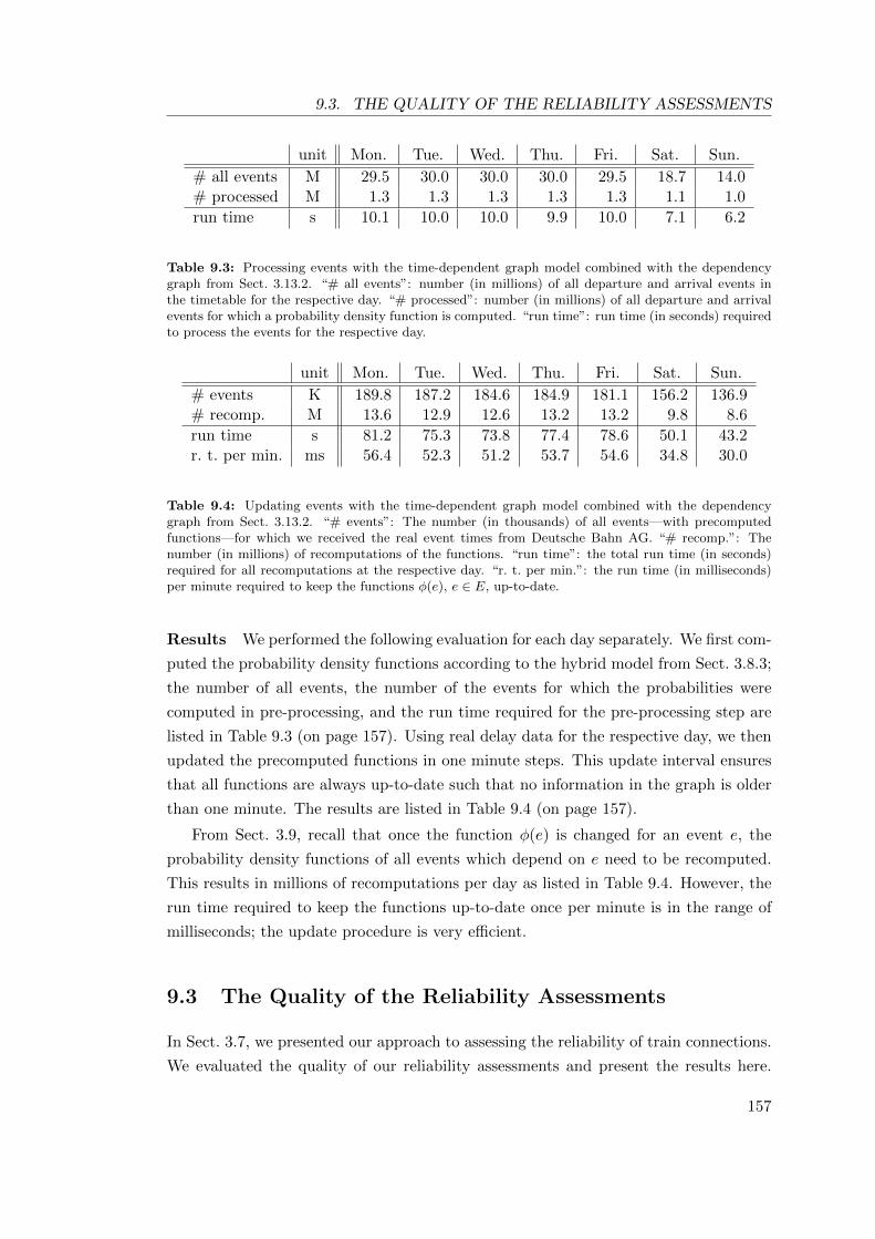
9.3. THE QUALITY OF THE RELIABILITY ASSESSMENTS
unit Mon. Tue. Wed. Thu. Fri. Sat. Sun.
# all events M 29.5 30.0 30.0 30.0 29.5 18.7 14.0# processed M 1.3 1.3 1.3 1.3 1.3 1.1 1.0
run time s 10.1 10.0 10.0 9.9 10.0 7.1 6.2
Table 9.3: Processing events with the time-dependent graph model combined with the dependencygraph from Sect. 3.13.2. “# all events”: number (in millions) of all departure and arrival events inthe timetable for the respective day. “# processed”: number (in millions) of all departure and arrivalevents for which a probability density function is computed. “run time”: run time (in seconds) requiredto process the events for the respective day.
unit Mon. Tue. Wed. Thu. Fri. Sat. Sun.
# events K 189.8 187.2 184.6 184.9 181.1 156.2 136.9# recomp. M 13.6 12.9 12.6 13.2 13.2 9.8 8.6
run time s 81.2 75.3 73.8 77.4 78.6 50.1 43.2r. t. per min. ms 56.4 52.3 51.2 53.7 54.6 34.8 30.0
Table 9.4: Updating events with the time-dependent graph model combined with the dependencygraph from Sect. 3.13.2. “# events”: The number (in thousands) of all events—with precomputedfunctions—for which we received the real event times from Deutsche Bahn AG. “# recomp.”: Thenumber (in millions) of recomputations of the functions. “run time”: the total run time (in seconds)required for all recomputations at the respective day. “r. t. per min.”: the run time (in milliseconds)per minute required to keep the functions φ(e), e ∈ E, up-to-date.
Results We performed the following evaluation for each day separately. We first com-
puted the probability density functions according to the hybrid model from Sect. 3.8.3;
the number of all events, the number of the events for which the probabilities were
computed in pre-processing, and the run time required for the pre-processing step are
listed in Table 9.3 (on page 157). Using real delay data for the respective day, we then
updated the precomputed functions in one minute steps. This update interval ensures
that all functions are always up-to-date such that no information in the graph is older
than one minute. The results are listed in Table 9.4 (on page 157).
From Sect. 3.9, recall that once the function φ(e) is changed for an event e, the
probability density functions of all events which depend on e need to be recomputed.
This results in millions of recomputations per day as listed in Table 9.4. However, the
run time required to keep the functions up-to-date once per minute is in the range of
milliseconds; the update procedure is very efficient.
9.3 The Quality of the Reliability Assessments
In Sect. 3.7, we presented our approach to assessing the reliability of train connections.
We evaluated the quality of our reliability assessments and present the results here.
157

CHAPTER 9. COMPUTATIONAL STUDY
Briefly, we evaluated a large set of train connections. We first assessed the reliability of
each train connection prior to the time when the real event times become known. We
then checked the feasibility of each train connection according to the real event times
which were known to us owing to Deutsche Bahn AG. This comparison allowed us an
evaluation of the quality of our reliability assessments. In the following, we explain the
evaluation procedure more precisely.
The procedure The evaluation procedure was is follows.
• The setup process to model the timetable is exactly as in Sect. 9.2.2.
• After the setup, for each day from 21 to 27 November 2016, we randomly created a
number of 100,000 queries consisting of a departure station, a destination station,
and a one hour time interval for the departure. We obtained 700,000 queries in
total.
• Using our timetable information system MOTIS, we computed the set of all Pareto
optimal train connections (cf. Sect. 2.2) for each query; travel time and number
of transfers were the Pareto criteria. We obtained 1,183,174 train connections in
total.
• We computed the probability of the success of each of the train connections by
our method for reliability assessment from Sect. 3.7. On average, our method
required 317 microseconds to compute the probability of the success of a train
connection.
• Last, for each train connection, we checked its feasibility according to real event
times (cf. Sect. 1.3.2) using real delay data—from Deutsche Bahn AG—for the
period from 21 to 27 November 2016. More precisely, for each transfer activity
(earr, edep) in each of the train connections, we checked whether
real(earr) + min dur(earr, edep) ≤ real(edep)
is true. In words, we checked whether passengers had sufficient time to transfer
from the first train to the second one.
The feasibility of a train connection—according to real times—can be verified only if,
for each transfer activity (earr, edep) in the train connection, the real times of earr and
edep are known to us. From Deutsche Bahn AG, we did not receive the real times of all
events in the timetable. We consequently could not check the feasibility of many train
connections which we had computed in the second step of the evaluation procedure. In
158

9.3. THE QUALITY OF THE RELIABILITY ASSESSMENTS
0 0.25 0.5 0.75 1
10
20
30
40
Figure 9.1: The x-axis represents the values for the probability of success computed by our reliabilityassessment method. The y-axis represents the percentage of the train connections. The green and thered histograms are computed over all train connections which were feasible and infeasible according toreal event times respectively.
total, we could verify the feasibility of 136,601 train connections; this builds the set of
train connections for the rest of our computational study in the following.
Results In Fig. 9.1 (on page 159) and Fig. 9.2 (on page 160), we analyze our reliability
assessments (the probabilities of success) for the train connections which were feasible
according to the real times as well as for the train connections which were infeasible.
The results demonstrate that our method for reliability assessment frequently delivered
high probabilities of success for train connections which were actually feasible according
to real event times. Train connections which broke usually had lower probabilities of
success.
Note: On average, the evaluated train connections had scheduled travel times of 351
minutes and 2.8 transfer activities (cf. Sect. 1.2).
Receiver operating characteristic For a further quality measurement of our
method for reliability assessment, we computed the receiver operating characteristic
(ROC) curve [Faw06]. Fig. 9.3 (on page 161) demonstrates the result; the area under
the curve (AUC) equals 0.81. This curve is computed as follows.
For each ρ ∈ [0, 1] ⊂ R, for all train connections with a probability of success lower
than ρ, we predicted that they become infeasible according to the real event times;
for the rest, we predicted that they will be feasible according to the real event times.
The x-axis represents the false positive rate which equals FP/N; the y-axis represents
the true positive rate which equals TP/P; these values are defined as follows. FP is
159

CHAPTER 9. COMPUTATIONAL STUDY
0 0.25 0.5 0.75 1
25
50
75
100
feasible; ≤ ρfeasible; ≥ ρ
infeasible; ≤ ρinfeasible; ≥ ρ
Figure 9.2: The x-axis represents the values for the probability of success ρ ∈ [0, 1] ⊂ R computed byour reliability assessment method. The y-axis represents the percentage of the train connections. Thegreen and the red curves are computed over all train connections which were feasible and infeasibleaccording to real event times respectively. The solid curves represent the percentage of the trainconnections with a probability of success lower than or equal to the respective value for ρ. The dashedcurves represent the percentage of the train connections with a probability of success greater than orequal to the respective value for ρ. To compute the curves, we evaluated 100 values for ρ and connectedthe measurement points.
the number of all feasible train connections (according to real event times) for which
our predictions were incorrect. TP is the number of all infeasible train connections
(according to real event times) for which our predictions were correct. N and P are the
numbers of all train connections which were feasible and infeasible according to real
event times respectively. For a better understanding, the function y = x represents the
prediction strategy to guess randomly [Faw06].
Discussion The evaluation demonstrates that our reliability assessments are accurate
and precise to a significant extent. However, we believe that better results can be
obtained by our reliability assessment method as follows.
• The quality of our reliability assessments strongly depends on the quality of the
input data used for the random prepared times and the random train move du-
rations. The functions which we used for this evaluation were not as accurate as
desired; we even had to generate some functions as explained in Sect. 9.1. An
incorporation of information about the tracks and the stations of the train moves
could improve the quality of the reliability assessments (cf. Sect. 3.4).
• The maximum waiting times (cf. Sect. 1.3.2) which we could use as input data
were not exactly the same as applied by Deutsche Bahn AG. We found out that
160
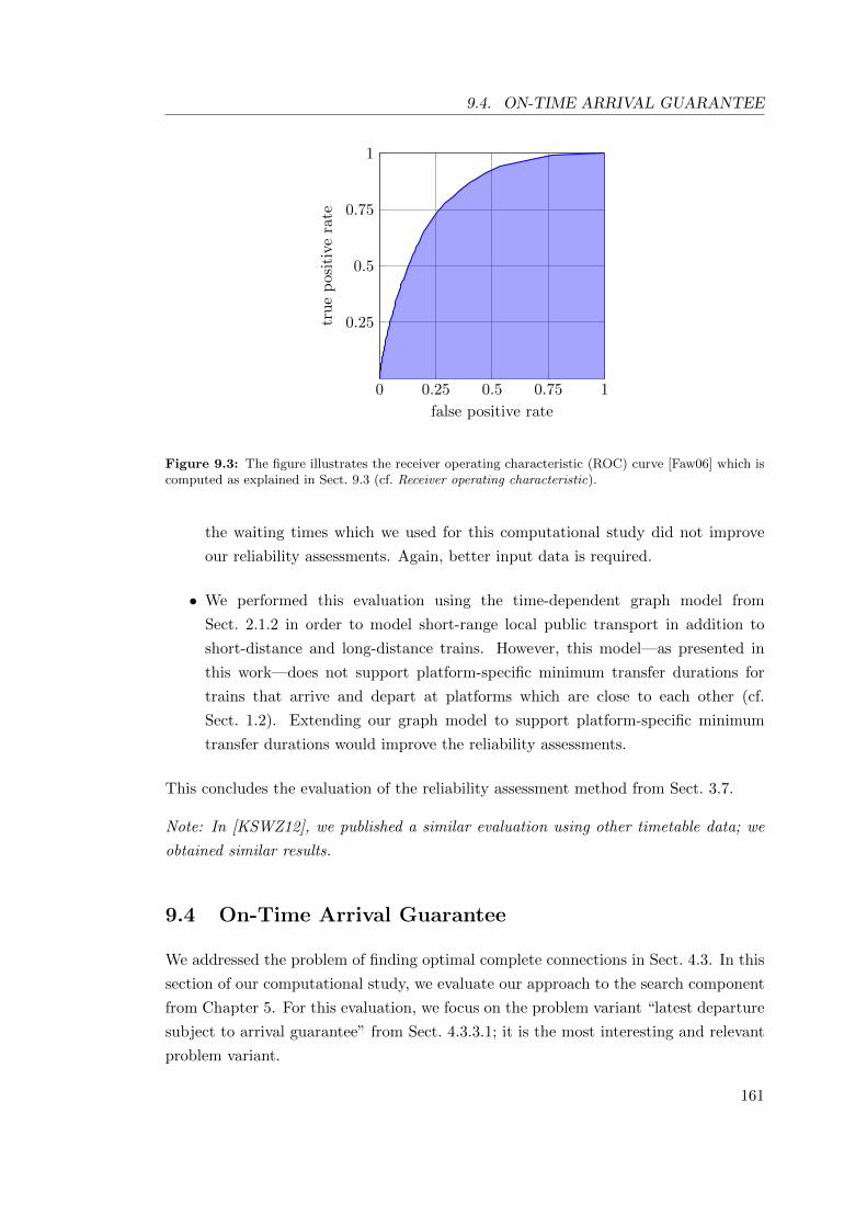
9.4. ON-TIME ARRIVAL GUARANTEE
0 0.25 0.5 0.75 1
0.25
0.5
0.75
1
false positive rate
tru
ep
osi
tive
rate
Figure 9.3: The figure illustrates the receiver operating characteristic (ROC) curve [Faw06] which iscomputed as explained in Sect. 9.3 (cf. Receiver operating characteristic).
the waiting times which we used for this computational study did not improve
our reliability assessments. Again, better input data is required.
• We performed this evaluation using the time-dependent graph model from
Sect. 2.1.2 in order to model short-range local public transport in addition to
short-distance and long-distance trains. However, this model—as presented in
this work—does not support platform-specific minimum transfer durations for
trains that arrive and depart at platforms which are close to each other (cf.
Sect. 1.2). Extending our graph model to support platform-specific minimum
transfer durations would improve the reliability assessments.
This concludes the evaluation of the reliability assessment method from Sect. 3.7.
Note: In [KSWZ12], we published a similar evaluation using other timetable data; we
obtained similar results.
9.4 On-Time Arrival Guarantee
We addressed the problem of finding optimal complete connections in Sect. 4.3. In this
section of our computational study, we evaluate our approach to the search component
from Chapter 5. For this evaluation, we focus on the problem variant “latest departure
subject to arrival guarantee” from Sect. 4.3.3.1; it is the most interesting and relevant
problem variant.
161

CHAPTER 9. COMPUTATIONAL STUDY
Overview In Sect. 9.4.1, we specify the objectives of this evaluation. We discuss in
Sect. 9.4.2 and 9.4.3 how we proceeded to achieve these objectives. In Sect. 9.4.4, we
explain the setup data for the evaluation. In Sect. 9.4.5–9.4.10, we present and discuss
the evaluation results. Last, in Sect. 9.4.11 and 9.4.12, we evaluate the heuristics which
are applicable to our search approach as well as the effect of our methods of discovering
relevant events in order to accelerate the search.
9.4.1 Objectives of the Computational Study
Our computational study is based on a real-world, national train network (in Ger-
many) with real timetable data. From our computational study, we draw the following
conclusions:
1. If meeting the deadline is the primary criterion for the passenger, then (I) it must
be the sole primary criterion for the search component as well, and (II) alternative
continuations must be taken into account and optimized at the booking stage (cf.
Sect. 4.4).
2. State-of-the-art traffic information systems do not provide solutions for the prob-
lem specified in Sect. 4.3. To overcome this problem, some passengers choose
an attractive train connection—computed with no regard for the probability of
success—and change to the next available alternative continuation in case that
a transfer becomes infeasible due to delays. We demonstrate that this strategy
frequently yields suboptimal and even infeasible outcomes. Hence, it is well worth
the effort to search for optimal outcomes through our approach.
3. The simpler approach to incorporate buffer times at critical points in the journey
yields suboptimal outcomes.
4. Outcomes of our approach are attractive in terms of travel time and the number of
transfers. Thus, our approach delivers outcomes with a high travel convenience,
and may be attractive to passengers.
5. Our approach has efficient response times and is suitable from a practical point
of view.
In the rest of this section, we present the evaluations of the above claims.
9.4.2 The Evaluated Approaches
We evaluated the claims from Sect. 9.4.1 by comparing our optimal approach from
Chapter 5 to the alternative approaches from Sect. 7.1.1–7.1.3. In the following, we list
all evaluated approaches and review their outcomes for each query q (cf. Sect. 4.3.1).
162

9.4. ON-TIME ARRIVAL GUARANTEE
OPT We denote by OPT our optimal approach to the search component from Chap-
ter 5; we combined it with the recursive formula from Sect. 5.3 and the incremental
approach from Sect. 5.9. The approach OPT delivers the optimal complete connection
according to the objective function from Eq. 4.3.1 (on page 73).
Note: The approach OPT uses the recursive formula from Sect. 5.3; in Sect. 9.4.9, we
will additionally evaluate the extended recursive formula from Sect. 5.4.
DP-L This approach has been introduced in Sect. 7.1.1; without regard for probabil-
ity of success, it delivers the train connection with the latest scheduled departure time
at dep st(q). We compare OPT to this approach in order to verify the first and the
fourth claim from Sect. 9.4.1.
DP-LP This approach has been introduced in Sect. 7.1.1; without regard for prob-
ability of success, it delivers the train connection with the latest scheduled departure
time at dep st(q) among Pareto optimal train connections. In Sect. 7.1.1, we introduced
the parameter δ to specify the time interval for the arrival at dest st(q); for δ, we used
100 minutes in our computational study. We compare OPT to this approach in order
to verify the first and the fourth claim from Sect. 9.4.1.
CEA This approach has been introduced in Sect. 7.1.3; it simulates the behavior
of passengers which is described in the second claim from Sect. 9.4.1. We introduced
in Sect. 7.1.3 the parameter δ in order to specify the time interval for the arrival at
dest st(q); for δ, we used 100 minutes in our computational study. We compare OPT
to this approach in order to verify the first and the second claim from Sect. 9.4.1.
BT This approach has been introduced in Sect. 7.1.2; it delivers the train connection
with the latest scheduled departure time at dep st(q) such that a minimum buffer time
is satisfied for each transfer and prior to the deadline at dest st(q). The minimum buffer
time as required for BT was denoted by τ in Sect. 7.1.2. In our computational study,
we evaluated τ ∈ {10, 15, 20, 30} (in minutes); we denote these approaches by BT-10 ,
BT-15 , BT-20 , and BT-30 respectively. We compare OPT to this approach in order
to verify the third claim from Sect. 9.4.1.
Applied heuristics For OPT as well as for all approaches for comparison, we applied
the heuristic “maximum waiting time of passengers” from Sect. 5.11.1; we limited the
maximum waiting time at a station for a transfer to 150 minutes. This is the only
heuristic used for OPT in the evaluations presented in Sect. 9.4.5–9.4.9. We will discuss
the effect of the heuristics from Sect. 5.11 in Sect. 9.4.11.
163

CHAPTER 9. COMPUTATIONAL STUDY
Note: Equally for all approaches, we dropped negligible probabilities as discussed in
Sect. 3.13.3 and 9.2.1.
9.4.3 Classifying the Outcomes
In the previous section, we listed the approaches we evaluated. For each query q,
the outcome of each of the approaches OPT and CEA is a complete connection as
specified in Sect. 4.3.2; the outcome of each of the approaches DP-L, DP-LP , and BT
is a train connection as specified in Sect. 1.2. In order to evaluate the approaches,
we mainly focused on two relevant properties of their outcomes: probability of success
and scheduled departure time. For complete connections, both properties have been
discussed in Sect. 5.5. For train connection, the scheduled departure time has been
introduced in Sect. 1.2; the probability of success is computed by the method from
Sect. 3.7.2.
From Sect. 4.3.1, recall that, for a query q, the value ρreq(q) denotes the probability of
success required by q. Moreover, the value ρ(o) denotes the probability of success of the
outcome o of an approach—the outcome o is either a train connection or a complete
connection. For each evaluated query q, we classified the outcome o of each approach
as follows:
• void : if the approach did not deliver any outcome to the query, its outcome is
called void ;
• infeasible: the outcome o is called infeasible if ρ(o) < ρreq(q);
• feasible: the outcome o is called feasible if ρ(o) ≥ ρreq(q).
Furthermore, feasible outcomes are sub-classified as follows:
• optimal : a feasible outcome is called optimal if there was no other feasible outcome
for query q which had a later scheduled departure time at dep st(q);
• suboptimal : a feasible outcome is called suboptimal if there was at least one
other feasible outcome for query q which had a later scheduled departure time at
dep st(q).
The approaches OPT and CEA deliver outcomes which are either feasible or void while
DP-L, DP-LP , and BT even deliver infeasible outcomes for some queries.
To avoid misunderstandings: In Chapter 3 and Sect. 9.3, we used the terms “feasible”
and “infeasible” in a different context and with a different meaning. In Sect. 9.4, the
terms “feasible” and “infeasible” are defined according to Sect. 4.3.
164
9.4. ON-TIME ARRIVAL GUARANTEE
9.4.4 Evaluation Setup and Test Queries
Timetable Using real timetable data from German railways, we prepared a time-
expanded graph (cf. Sect. 2.1.1) for a two days period, 5-6 August 2014, with 2.2M
departure and arrival nodes. This two days period allowed us to evaluate complete
connections that start and end at the same day as well as complete connections that end
at the very next day. We extended our time-expanded graph as discussed in Sect. 3.13.1
in order to provide an access to the functions φ(e), e ∈ E, and the interdependencies
between the events in constant time.
Queries The queries (cf. Sect. 4.3.1) for the computational study were designed as
follows. As departure and destination stations of the queries, we used 8,000 different
station pairs extracted from real customer queries (provided by German railways). We
combined each station pair with 10 different deadlines for the arrival at the destination:
deadline(q) ∈{
14:00, 17:00, 19:00, 21:00, 23:00,
01:00, 07:00, 08:00, 11:00, 13:00}
where the first five deadlines were on the first day and the last five deadlines were on
the second day of the timetable’s two-days period. This setting yielded 80,000 triples,
each consisting of a departure and a destination station as well as a deadline. We
combined each triple with five different values for the required probability of success:
ρreq(q) ∈{
0.95, 0.96, 0.97, 0.98, 0.99}.
We finally obtained 400,000 queries in total.
9.4.5 The Outcomes
We processed all queries, specified in Sect. 9.4.4, with our optimal approach OPT as
well as with all alternative approaches from Sect. 7.1. The results of this evaluation
are detailed in the following and in the rest of Sect. 9.4.
Feasibilities of the outcomes For each query, our approach OPT always delivered
the optimal outcome unless there was no feasible one (details about the heuristic from
Sect. 5.11.1 will be explained later in Sect. 9.4.11). For 5.3% of all queries, there were
no feasible outcomes; thus, the outcomes of OPT were void. It comes as no surprise
that for these queries no other approach could deliver feasible outcomes either.
In Table 9.5 (on page 166), we evaluate the feasibilities of the outcomes of the
alternative approaches from Sect. 7.1. More precisely, for each alternative approach,
we compare “the percentage of the queries for which the approach—as well as OPT—
delivered feasible outcomes” to “the percentage of the queries for which OPT was
165

CHAPTER 9. COMPUTATIONAL STUDY
ρ(q) outcomeD
P-L
DP-LP
BT-10
BT-15
BT-20
BT-30
CEA
99%OPT solely 59.8 59.8 16.8 8.7 5.1 5.5 12.8both feasible 34.9 32.9 77.9 86.0 89.6 89.2 79.9
98%OPT solely 55.3 55.6 10.7 5.2 4.4 5.5 10.6both feasible 39.4 37.1 84.0 89.5 90.3 89.2 82.1
97%OPT solely 52.3 52.8 7.8 4.2 4.2 5.4 9.3both feasible 42.4 39.9 86.9 90.5 90.5 89.3 83.4
96%OPT solely 49.7 50.3 5.8 3.9 4.2 5.4 8.4both feasible 45.0 42.4 88.9 90.8 90.5 89.3 84.3
95%OPT solely 47.3 47.9 4.7 3.7 4.1 5.4 7.6both feasible 47.4 44.8 90.0 91.0 90.6 89.3 85.1
Table 9.5: The outcomes of the approaches: The number in each cell is the percentage of all querieswith the ρ(q)-value as listed in the first column (i.e. 80k queries for each ρ(q)-value).“OPT solely”: queries for which OPT delivered feasible—and necessarily optimal—outcomes while theoutcomes of the respective approach for comparison were either void or infeasible.“both feasible”: queries for which OPT and the respective approach for comparison delivered feasibleoutcomes.Note that, for 5.3% of the queries, no approach could deliver feasible outcomes. Moreover, for thecomparison of OPT to DP-LP and CEA, 2.0% of the queries have been excluded as explained inSect. 9.4.5 (cf. Excluded queries).
the only approach that delivered feasible outcomes”. We can see that the alternative
approaches have performances inferior to OPT .
Excluded queries From Sect. 7.1.1 and 7.1.3, recall that DP-LP and CEA use a
time interval for the arrival at dest st(q). To obtain a fair and valid comparison to
OPT , we excluded each query for which the outcomes of CEA/DP-LP and OPT were
as follows: DP-LP and CEA failed to find any Pareto optimal train connection arriving
at dest st(q) within the defined arrival interval while OPT delivered an outcome with
an alternative continuation arriving at dest st(q) earlier than this time interval. These
were 2.0% of all queries; thus, in Table 9.5 (on page 166), the percentages in the
respective cells (plus 5.3% for the queries without any feasible outcomes) add up to
98%. These queries are only excluded from the comparison of OPT to DP-LP and
CEA and not from the rest of our computational study. Note that for the excluded
queries the outcomes of OPT were optimal.
In Sect. 9.4.6–9.4.10, we discuss the objectives of our computational study from
Sect. 9.4.1 and give empirical evidence for them.
166

9.4. ON-TIME ARRIVAL GUARANTEE
ρ(q) OPT BT-10 BT-15 BT-20 BT-30 CEA
99% 100.0 56.8 39.9 29.1 17.1 76.098% 100.0 53.8 37.2 26.9 15.9 77.197% 100.0 51.8 35.6 25.8 15.2 77.896% 100.0 50.3 34.3 24.8 14.7 78.495% 100.0 48.9 33.4 24.1 14.3 78.9
Table 9.6: Optimality evaluation: For each approach, the table reports how often the feasible outcomeswere optimal. The numbers are percentages computed over all feasible outcomes of the respectiveapproach.
9.4.6 Relevance of Probability of Success and Optimality
Relevance of probability of success The evaluation of the outcomes of DP-L,
DP-LP , and CEA supports our first claim from Sect. 9.4.1. Table 9.5 (on page 166)
demonstrates that for about half of all queries, the approaches DP-L and DP-LP de-
livered infeasible outcomes while feasible outcomes existed (cf. “OPT solely”). Even
the CEA approach failed to deliver feasible outcomes for a significant number of the
queries. We conclude that for the problem from Sect. 4.3, where a probability of suc-
cess has to be guaranteed, the probability of success must be the primary criterion for
the search. Moreover, alternative continuations must be optimized already during the
search.
Relevance of optimality Our second claim from Sect. 9.4.1 is proven by the compar-
ison of OPT to the approach CEA. Above, we already demonstrated that CEA failed
to deliver feasible outcomes while feasible complete connections existed. We now focus
on the optimality of the feasible outcomes of CEA. For this, as presented in Table 9.6
(on page 167), we evaluated how often the feasible outcomes of each approach were
actually optimal. As listed in Tables 9.5 and 9.6, for a significant number of queries,
the CEA approach failed to deliver optimal or even any feasible outcomes. Moreover,
details about the differences between the departure times of the outcomes of OPT and
CEA can be found in Fig. 9.4 (on page 168). Compared to CEA, our approach OPT
delivered complete connections with significantly better—i.e. later—departure times.
Altogether, we can see that it is well worth the effort to search for optimal out-
comes with our dynamic programming approach OPT ; the strategy of the passengers
simulated by CEA is inferior to our optimal approach OPT .
9.4.7 Minimum Buffer Times
We now address our third claim from Sect. 9.4.1. Table 9.5 (on page 166) demonstrates
that the BT approach delivers feasible outcomes for quite a large fraction of the queries
167

CHAPTER 9. COMPUTATIONAL STUDY
0 60 120 180 240 300 360
1
10
100
1k
10k
100k
(a) BT-100 60 120 180 240 300 360
1
10
100
1k
10k
100k
(b) BT-15
0 60 120 180 240 300 360
10
100
1k
10k
100k
(c) BT-200 60 120 180 240 300 360
10
100
1k
10k
100k
(d) BT-30
0 60 120 180 240 300 360
1
10
100
1k
10k
100k
(e) CEA0 60 120 180 240 300 360
25%
50%
75%
100%
CEA
BT-10
BT-15
BT-20
BT-30
(f) BT and CEA
Figure 9.4: Detailed differences between the departure times of OPT ’s optimal outcomes comparedto the departure times of the feasible outcomes of BT and CEA. For each query q, the value δ (inminutes) equals “the departure time of OPT ’s outcome” minus “the departure time of the outcome ofBT/CEA”. For each value for δ, each of the histograms (a)–(e) illustrates the absolute number of thequeries with that δ-value. The figure (f) is a cumulative plot; the x-axis represents the values for δ;the y-axis represents the percentage of the queries with δ-values smaller than or equal to the respectiveδ-value on the x-axis. The maximum value illustrated for δ is 360. There are 706, 1197, 1846, 3345, and4 outcomes of the approaches BT-10 , BT-15 , BT-20 , BT-30 , and CEA that are not illustrated (theyhave a δ-value greater than 360). Each histogram in the figure comprises all queries for which OPTas well as BT/CEA delivered a feasible outcome (cf. Table 9.5 (on page 166)). These figure comprisessolely the queries with ρ(q) = 98% (we obtained similar results for the other values for ρ(q)). For thehistograms (a)-(e), the y-axis has a logarithmic scale.
168

9.4. ON-TIME ARRIVAL GUARANTEE
ρ(q) earlier average median
99% 49.1% 0.13 0.098% 44.2% 0.12 0.097% 41.0% 0.10 0.096% 38.3% 0.10 0.095% 36.0% 0.09 0.0
ρ(q) earlier average median
99% 77.6% 0.21 0.1398% 75.6% 0.20 0.1197% 74.1% 0.19 0.1196% 72.9% 0.18 0.1095% 72.1% 0.18 0.09
Table 9.7: The price of the on-time arrival guarantee; more precisely, the table reports on the earlierdeparture times of optimal outcomes (computed by OPT ) compared to the latest departure timeswithout regard for probability of success (computed by DP-L). The left table evaluates all queries forwhich the outcomes of DP-L were either feasible or infeasible. The right table evaluates only thosequeries for which the outcomes of DP-L were infeasible.“earlier”: queries for which the optimal outcomes of OPT depart earlier than the infeasible outcomesof DP-L; the numbers are percentages of all evaluated queries.“average”: the relative duration increase, as defined in Sect. 9.4.8, averaged over all evaluated queries.“median”: the median of the relative duration increase, over all evaluated queries.
but not as frequent as OPT . The superiority of OPT over BT becomes more clear
when comparing the departure times of the outcomes of both approaches. Table 9.6
(on page 167) focuses on this comparison; the results reveal that the BT approach fre-
quently delivered suboptimal outcomes. Moreover, in Fig. 9.4 (on page 168), histograms
demonstrate the detailed differences between the departure times of OPT and the BT
approach. As we can see, OPT delivered significantly better—i.e. later—departure
times for a large number of the queries. So, our computational study suggests that our
third claim from Sect. 9.4.1 is valid.
9.4.8 The Price of On-Time Arrival Guarantee
So far, we have demonstrated that OPT delivers complete connections which guaran-
tee the required probability of success and have scheduled departure times as late as
possible. We now discuss the price of this on-time arrival guarantee; more precisely,
we analyzed how much earlier departure times must be accepted by the passengers in
order to meet the required probability of success. For this, we compared the departure
times of the outcomes of OPT to the departure times of the outcomes of DP-L; recall
that, without regard for probability of success, the latter delivers the latest departure
time such that an arrival prior to the deadline is still possible.
The results of this evaluation are illustrated in Table 9.7 (on page 169) and Fig. 9.5
(on page 170). There, for each query q, the minimum duration denotes the absolute
difference between deadline(q) and the scheduled departure time of the outcome of
DP-L for the query q. Moreover, the duration increase denotes the absolute time
difference between the scheduled departure times of the outcomes of OPT and DP-L
for the query q. The relative duration increase denotes the ratio of duration increase
169

CHAPTER 9. COMPUTATIONAL STUDY
0 15 30 45 60 75 90 105 120 135 150
1
10
100
1k
10k
100k
Figure 9.5: The price of the on-time arrival guarantee; more precisely, the histogram reports onthe earlier departure times of optimal outcomes (computed by OPT ) compared to the latest departuretimes without regard for probability of success (computed by DP-L). For each value for relative durationincrease, as defined in Sect. 9.4.8, the histogram illustrates the number of the queries with that value;the values are multiplied by 100 for better readability. The maximum value that is illustrated in thehistogram is 150; there are 581 (=0.7%) outcomes that are not illustrated since they have a valuegreater than 150. The histogram comprises all queries where the outcomes of OPT were optimal andthe outcomes of DP-L were either feasible or infeasible. The histogram is exemplary; solely for querieswith ρ(q) = 98% (we obtained similar results for the other values for ρ(q)). The y-axis has a logarithmicscale. For more details, we refer to Table 9.7 (on page 169).
to minimum duration.
For a fraction of the queries where the outcomes of DP-L were infeasible, we see
that earlier departure times—such as computed by OPT—must be accepted in order
to guarantee the required probability of success ρreq(q). For these queries, there were
no feasible outcomes with later departure times. On the other hand, for all queries
where DP-L delivered feasible outcomes, the departure times of the outcomes of OPT
and DP-L were the same. As Table 9.7 (on page 169) reports, averaged over all queries
for which DP-L delivered feasible or infeasible outcomes, the relative duration increase
is acceptable. Moreover, OPT still delivered better departure times compared to the
alternative approaches BT and CEA.
The approach OPT consequently computes outcomes with an on-time arrival guar-
antee and travel times which are still attractive even for busy people. The comparison
above was the first step to prove the fourth claim from Sect. 9.4.1; in Sect. 9.4.9, we
present further evaluations of the criteria travel time and number of transfers.
9.4.9 Travel Convenience
In the previous section, we discussed the price of the on-time arrival guarantee. In this
section, we further on address the fourth claim from Sect. 9.4.1; we analyze the number
of transfers and the travel time of the outcomes. For train connections, both properties
are defined as described in Sect. 1.2; for complete connections, both are expected values
as explained in Sect. 5.5.
The approach OPT optimizes these properties as secondary criteria; more precisely,
they are used as tie-breakers. In Sect. 5.3 and 5.4, we presented two recursive functions
170

9.4. ON-TIME ARRIVAL GUARANTEE
OPT
-1
OPT
-2
DP-L
DP-LP
BT-10
BT-15
BT-20
BT-30
CEA
transfers 1.6 1.7 1.7 1.8 1.6 1.5 1.5 1.5 1.5durations 257 247 244 240 273 283 293 311 291
Table 9.8: The number of transfers and the travel times (in minutes) of the approaches, averagedover all (feasible and infeasible) outcomes of each approach.“OPT-1”: our optimal approach OPT with the recursive function from Sect. 5.3, the number oftransfers as tie-breaker, and a tolerance of 10−4 for the comparison of the probabilities as explained inSect. 5.3.4; see Table 9.9 (on page 171) for the evaluation of further tolerance values.“OPT-2”: our optimal approach OPT with the extended recursive function from Sect. 5.4, the weightedsum as described in Sect. 9.4.9 as tie-breaker, and a tolerance value of 10−4 for the comparison of theprobabilities.Note: The expected travel time of the outcomes of OPT-1 could only be computed by the recursivefunction from Sect. 5.4 in a post-processing step after the computation of the outcomes.
tolerance 0 10−5 10−4
transfers 3.3 1.7 1.6suboptimal 0% 0.0065% 0.04%
Table 9.9: The expected number of transfers of OPT ’s outcomes obtained by the recursive functionfrom Sect. 5.3, averaged over all feasible outcomes.“tolerance”: the tolerance value for the comparison of the probabilities as described in Sect. 5.3.4.“transfers”: the expected number of transfers of the complete connections (on average).“suboptimal”: the percentage of the queries for which OPT delivered suboptimal outcomes because ofthe applied tolerance.
that compute optimal complete connections; the first one allows us to optimize the
number of transfers as a secondary criterion (cf. Sect. 5.3.4); the second one allows
us to optimize a weighted sum of the number of transfers and the travel time as a
secondary criterion (cf. Sect. 5.4.2). Both are evaluated in the following.
Optimizing number of transfers solely By the recursive formula from Sect. 5.3,
we optimized the number of transfers as the secondary criterion. The results are listed
in Table 9.8 (on page 171); see the values for OPT-1 . We evaluated different tolerance
values as discussed in cf. Sect. 5.3.4; the results are presented in Table 9.9 (on page 171).
We see that the evaluated tolerance values significantly reduce the expected number
of transfers but affect the optimality only marginally. As claimed in Sect. 9.4.1, OPT
delivers outcomes with attractive numbers of transfers, comparable with DP-L and
DP-LP .
Optimizing number of transfers and travel time We evaluated the extended
recursive function from Sect. 5.4. As tie-breaker, we used the weighted sum from
Eq. 5.4.5 (on page 90); for each arrival event earr and some time t ∈ supp(φ(earr)), if
171

CHAPTER 9. COMPUTATIONAL STUDY
two or more successors obtain the maximum probability of success, recall that we select
the successor with the better weighted sum. In the weighted sum, we set the weight
wa = 1; the weight wt for the number of transfers is set to
wt = max{
15.0, 0.15 ·(deadline(q)− sched(earr)
) }where earr is the arrival event for which we determine the best successors according to
Eq. 5.4.1 (on page 88). In words, the weighted sum requires that each additional transfer
decreases the expected travel time by 15% of the time difference between deadline(q)
and sched(earr) but at least by 15 minutes.
The results are presented in Table 9.8 (on page 171); see the values for OPT-2 . As
claimed in Sect. 9.4.1, OPT delivers outcomes with attractive travel times, comparable
with DP-L and DP-LP .
Note: Recall that the expected travel time can only be computed using the extended
recursive function from Sect. 5.4. In order to see the improvement of the travel times
obtained by that approach compared to the approach from Sect. 5.3, we calculated the
travel times of the outcomes obtained by the recursive function from Sect. 5.3 in a post-
processing step using the extended recursive function from Sect. 5.4. This calculation
can be accomplished analogous to an ex-post calculation of the probability of the success
of a complete connection as explained in Sect. 6.2.2.1 (cf. Recalculation of the probability
of success).
9.4.10 Efficiency and Practicability
We finally address the last claim from Sect. 9.4.1. The response times of the approaches
are listed in Table 9.10 (on page 173). For OPT , this table lists the response times which
are obtained by applying our incremental approach from Sect. 5.9. We listed the times
for all 80k queries with ρreq(q) = 98% as an example; for all approaches for comparison,
we measured similar response times for the other values for ρreq(q); for OPT , we noticed
3-4% longer response times when processing queries with ρreq(q) = 99% compared to
queries with ρreq(q) = 95%.
We see that the optimization of the travel time by the extended recursive formula
from Sect. 5.4 is more expensive than applying the recursive function from Sect. 5.3;
which recursive function is more appropriate, should be decided depending on the
requirements and preferences of the passengers.
A desktop PC as specified in Sect. 9.4.4 is sufficient to run up to four instances of
our implementation of OPT in parallel. The results presented in this section and the
average response time of 2.0s are indicative that our optimal approach OPT is efficient
and practicable as claimed in Sect. 9.4.1.
172

9.4. ON-TIME ARRIVAL GUARANTEE
OPT
-1
OPT
-2
DP-L
DP-LP
BT-10
BT-15
BT-20
BT-30
CEA
average 2,025 2,477 157 183 171 171 169 169 1,59490%-q. 4,773 5,424 329 396 366 364 360 364 3,369
Table 9.10: For each approach, the table lists the average response time as well as the 90%-quantileof the response times over all 80k queries with ρ(q) = 98%. All times are in milliseconds.“OPT-1”: our optimal approach OPT with the recursive function from Sect. 5.3.“OPT-2”: our optimal approach OPT with the extended recursive function from Sect. 5.4.“average”: the response time of the respective approach on average.“90%-q.”: the 90%-quantile of the response times of the respective approach.
9.4.11 Heuristics
In this section, we discuss the evaluation of the heuristics from Sect. 5.11. The only
heuristic we used in our evaluations presented in Sect. 9.4.5–9.4.10 was “maximum
waiting time of passengers”.
Maximum waiting time of passengers In Sect. 5.11.1, we discussed the maximum
waiting time of passengers at a station for a transfer. This assumption and heuristic
results in suboptimal outcomes for about 2.3% of all queries when limiting the maximum
waiting time to 150 minutes. Fortunately, this loss of optimality is negligible as will be
explained in the following. For the optimal outcomes for these queries, the passengers
are expected to wait at some station for a time longer than 150 minutes; for 99% of these
outcomes, this waiting window is during the night (12:00 midnight – 05:00 a.m.). Such
journeys are not attractive, and, in such cases, passengers usually decide to travel a day
earlier or even by other means of transport. Moreover, in such cases, the suboptimal
outcomes which are computed by demanding a maximum waiting time are potentially
more attractive than the optimal ones that we miss; the passengers have the possibility
to sit or even sleep in a train instead of waiting at a station during the nighttime. In
summary, this loss of optimality is negligible.
Without this heuristic, our search component would have up to six times longer
response times on average. The time saving obtained by this heuristic has two main
reasons. First, the number of the events discovered as relevant (cf. set Eincrelevant in
Algorithm 5.4 on page 103) is reduced by about 14%. Second, the numbers of the
predecessors and successors of each event visited during the procedure of discovering
relevant events is significantly reduced.
The further heuristics We also evaluated the three heuristics from Sect. 5.11.2–
5.11.4: “earliest arrival time at the destination”, “earliest departure time”, and “cycles
through the departure station”. In this evaluation, we set the earliest arrival time for
173

CHAPTER 9. COMPUTATIONAL STUDY
each query q to deadline(q) − 100 minutes. The earliest departure time was set to
the earliest arrival time at the destination minus the travel time of the longest Pareto
optimal connection (cf. Sect. 2.2) that arrives no earlier than the earliest arrival time
at the destination and no later than deadline(q); the criteria optimized by this Pareto
search were travel time and number of transfers.
We evaluated these three heuristics not individually but together. Applying them
reduced the number of the events discovered as relevant (cf. set Eincrelevant in Algorithm 5.4
on page 103) by 7%. On the other side, these heuristics resulted in 3.9% queries with
suboptimal outcomes. The loss of optimality is significant such that the heuristics
from Sect. 5.11.2–5.11.4 do not confer an advantage on our incremental approach from
Sect. 5.9. Therefore, we did not use them in our evaluations presented in Sect. 9.4.5–
9.4.10.
9.4.12 The Discovery of Relevant Events
In Sect. 9.4.10, we presented and discussed the response times of our approach OPT
combined with the incremental approach from Sect. 5.9. In this section, we compare
our different methods of discovering relevant events from Sect. 5.8 and 5.9; we evaluated
three variants of our optimal approach OPT :
• OPT : the approach OPT combined with the incremental approach from Sect. 5.9,
• OPT-P : the approach OPT combined with the pre-processing method from
Sect. 5.8.2, and
• OPT-PE : the approach OPT combined with the pre-processing method from
Sect. 5.8.2 as well as the early termination from Sect. 5.7.2.
Exclusively for this evaluation, we used all heuristics from Sect. 5.11 for all three above
variants. The reason is that the set Erelevant of all relevant events (cf. Sect. 5.8) could be
very large such that the approaches OPT-P and OPT-PE—which discover all relevant
events in pre-processing—would be too expensive for the evaluated problem variant
from Sect. 4.3.3.1 (cf. Latest Departure Subject to Arrival Guarantee). Particularly
for OPT-P and OPT-PE , earliest arrival and departure times need to be defined in
order to significantly limit the number of discovered relevant events and facilitate an
evaluation of a large number of queries.
The results of the comparison are listed in Table 9.11 (on page 175). As we see, the
early termination from Sect. 5.7.2 significantly accelerates the response times. How-
ever, for the problem variant from Sect. 4.3.3.1 (cf. Latest Departure Subject to Arrival
Guarantee), our optimal approach OPT from Chapter 5 obtains efficient response times
when using the incremental approach from Sect. 5.9.
174

9.5. LATE-NIGHT CONNECTIONS
function OPT-P OPT-PE OPT
average timeSect. 5.4 10.0 6.8 1.2Sect. 5.3 4.3 3.5 1.0
90%-quantileSect. 5.4 11.7 7.7 1.1Sect. 5.3 5.0 4.0 1.0
#eventsSect. 5.4 16.9 11.2 1.0Sect. 5.3 16.9 11.2 1.0
Table 9.11: Comparison of the response times of OPT combined with the different methods ofdiscovering relevant events. All values are listed as multiples of the respective values for the approachOPT with our incremental approach from Sect. 5.9 and the recursive function from Sect. 5.3.“average time”: the response time of the respective approach on average.“90%-quantile”: the 90%-quantile of the response times of the respective approach.“#events”: the number of the events which have been processed by Algorithm 5.1 (on page 94).“function”: the recursive function applied to compute the outcomes.Note: We evaluated all 80k queries with ρ(q) = 98%.
Note: Without the heuristics, the speed-up factors would be even larger since OPT with
the incremental approach does not profit from the heuristics as much as the slower
variants OPT-P and OPT-PE.
9.5 Late-Night Connections
In this section, we present the evaluation of our approach of computing late-night
connections which has been discussed in Sect. 8.4. The evaluation setup is explained
in Sect. 9.5.1; the results are presented in Sect. 9.5.2.
9.5.1 Evaluation Setup
We first explain the evaluation procedure; we then discuss parameters and functions
we defined for this evaluation.
The procedure In short, we detected critical situations in the timetable; these are
situations where, after a (late) connection break, no attractive alternative continuations
to the destination could be found by employing the basic Pareto Dijkstra algorithm from
Sect. 2.2. For each critical situation, we applied our late-night connection search from
Sect. 8.4. We then compared the late-night connections to the alternative continuations
computed by the basic search from Sect. 2.2 in order to evaluate the performance of
our search approach. The evaluation procedure is detailed in the following.
1. First, we generated random queries as follows. We used the timetable from
Sect. 9.2.1 for the two-days period 21-22 November 2016. We generated a set
of 100,000 queries where each query was as defined in Sect. 2.2. For each query
175

CHAPTER 9. COMPUTATIONAL STUDY
q, as the time interval [begin(q), end(q)] for the departure, we randomly selected a
one hour time interval between 16:00 o’clock and 23:59 o’clock on November 21.
As departure and destination stations, we selected random train stations.
2. For each query, we computed the set of all Pareto optimal train connections by
employing the basic Pareto Dijkstra algorithm from Sect. 2.2; the travel duration
and the number of transfers were the Pareto criteria. We obtained 137,639 train
connections.
3. Among the train connections computed, we then selected the train connections
with late arrival times at the destination. More precisely, from the 137,639 train
connections computed in the previous step, we selected each train connection
with an arrival time between 16:00 o’clock on November 21 and 1:00 o’clock on
November 22. We obtained 6,891 train connections.
4. For each train connection c with a late arrival time, we simulated connection
breaks and detected critical situations as follows. For this purpose, for each
departure event edep in c, we assumed that the train move starting with edep
is not available anymore. By employing the basic Pareto Dijkstra algorithm
from Sect. 2.2 (in the on-trip scenario), we subsequently searched for alternative
continuation from the station of edep to the destination station of c; we call these
alternative continuations the basic alternative continuations. To perform this
search, we set ontrip time(q) = sched(edep) + 1.
For the train connection c and a basic alternative continuation computed, let t and
t′ respectively denote the arrival times of c and the basic alternative continuation
(the arrival time at the destination station); we continued as follows.
• If a basic alternative continuation could be found such that t′ − t < 60
minutes, we assumed that the passenger will take it, and the late-night
connection search would be pointless in that situation. Thus, we continued
with next departure events in the train connection c in order to find critical
situations.
• If no basic alternative continuation could be found such that t′− t < 60 min-
utes, a situation was detected where the basic search approach from Sect. 2.2
had failed to deliver an attractive alternative continuation. We collected all
these critical situations; in total, we found 73,999 critical situations.
5. For each critical situation detected in the previous step, we performed an on-trip
search by employing our late-night connection search from 8.4; the query was
specified as for the search for basic alternative continuations (see the previous
176

9.5. LATE-NIGHT CONNECTIONS
step). The search delivered late-night alternative continuations to the destination
station from the station where the original train connection c were assumed to
be broken.
6. For each situation detected in the fourth step, we then compared the basic al-
ternative continuations to the late-night alternative continuations. According to
the Pareto Dijkstra algorithm, for each query, a set of train connections is de-
livered. For the comparison, from the set of the basic alternative continuations
computed, we selected the alternative continuation with the earliest arrival time
at the destination station; in the rest of this section, we call this alternative
continuation the basic alternative continuation. From the set of the late-night
alternative continuations computed, we selected four alternative continuations as
follows:
• Earliest: the late-night alternative continuation with the earliest arrival time
at the destination station.
• Min. costs: the late-night alternative continuation minimizing the tp-costs
criterion (cf. Sect. 8.4.5).
• Min. night: the late-night alternative continuation minimizing the nighttime
criterion (cf. Sect. 8.4.5).
• Min. night*: the late-night alternative continuation minimizing the night-
time criterion among all late-night alternative continuations which had a
tp-cost not greater than the tp-cost of the basic alternative continuation.
The comparison results can be found in Sect. 9.5.2.
Model and parameters To facilitate this evaluation, we specified the following
parameters and functions.
• Delay compensation: According to [Bah16b], we assumed the following delay com-
pensation rule. The delay compensation is calculated depending on the scheduled
arrival time of the original, broken train connection at the destination and the
actual arrival time of the passenger at the destination. Let c denote the original
train connection that is broken in the evening hours. Let γ(c) and δ respec-
tively denote the price of c and the delay of the passenger for the arrival at
the destination—when taking an alternative connection to the destination. We
177

CHAPTER 9. COMPUTATIONAL STUDY
calculated the compensation as follows:
delay compensation(c) =
e0.0 if δ < 60,
γ(c)/4 if δ ∈ [60, 120), and
γ(c)/2 if δ ≥ 120.
• Estimating the ticket price: Since the functions of computing ticket prices, em-
ployed by Deutsche Bahn AG, are unknown to us, we estimated the ticket prices.
Let β(c) denote the straight-line distance (in kilometers) from the departure sta-
tion to the destination station of the train connection c for which the price should
be computed. We estimated the ticket price γ(c) of the train connection c as fol-
lows:
γ(c) = min{e123.0, β(c) · 1.5 · e0.30
}.
The factor 1.5 is applied as a correction factor since β(c) is a straight-line distance.
• Hotels: We incorporated into our model 36 hotels close to train stations [Int16].
We assumed a fixed price of e70.0 for an overnight stay at a hotel. We set the
parameters minimum stay duration and earliest check-out time to 7 hours and
7:00 o’clock respectively (cf. Sect. 8.4, Taxi transfers and hotel stays).
• Taxis: Given a destination station s, we computed taxi transfers to s from each
station that was in the 50km radius of s. These taxi transfers were incorporated
into the search for late-night connections (cf. Sect. 8.4.4). For a taxi transfer,
let β denote the straight-line distance (in kilometers) from the station where the
passenger is collected to the destination station. In order to estimate the duration
of the taxi transfer, we proceeded as follows. We assumed speeds of 40 km/h and
100 km/h in cities and on highways respectively. Moreover, we assumed that
a 5km distance of β is always traveled in cities, and the remaining distance is
covered on highways. Hence, we obtain:
βcity = min{β, 5km}
and
βhighway = max{β − 5km, 0}
where
βcity + βhighway = β.
We estimated the duration (in minutes) of the taxi transfer by the following
178

9.5. LATE-NIGHT CONNECTIONS
function:
duration = 10min +( βcity
40km/h+
βhighway
100km/h
)· 1.5 · 60min/h.
In the formula above, 10 minutes is the time required to move from the train
station to the taxi as well as for entering and leaving the taxi. The factor 1.5 is
applied as a correction factor since β is a straight-line distance.
The price of the taxi transfer is computed by the following function:
price = e2.50 + β · 1.5 · e2.00.
We assumed that the transportation company can provide taxi transfers in the
time between 20:00 o’clock and 04:00 o’clock (on the very next day).
• Nighttime: We defined the time between 01:00 o’clock and 06:00 o’clock as the
nighttime (cf. Sect. 8.4.5, The nighttime criterion); recall that traveling in this
time period is undesired by passengers.
9.5.2 Results
We compared the basic alternative continuation—with the earliest arrival time at the
destination—to four late-night alternative continuations as specified in the sixth step
of the evaluation procedure in Sect. 9.5.1. The results are presented in Table 9.12 (on
page 180) as well as in Fig. 9.6 and 9.7.
Tp-costs and nighttime Compared to the basic alternative continuation, the tp-
cost (cf. Sect. 8.4.5) is reduced by 13% when taking the late-night alternative continua-
tion with the minimum tp-cost. A higher reduction of the tp-cost could not be obtained
since hotels and taxis are associated with costs (in addition to a delay compensation).
Note that a overnight stay at a hotel costs e70,0; in addition, the maximum delay
compensation has to be paid since the traveler reaches the destination with a delay of
more than two hours.
The travel time during nighttime can be reduced by 92% when taking the late-night
alternative continuations that minimizes the nighttime criterion. This is a significant
improvement from the point of view of the travelers. On the other side, such alternative
continuations use taxis and hotels; this consequently results in higher costs to be paid by
the transportation company—more than twice as high as the earliest basic alternative
continuation.
Note: In many cases, the tp-cost—to be paid by the transportation company—is mini-
179

CHAPTER 9. COMPUTATIONAL STUDY
basic earliest min. min. min.
alt. arrival costs night night*
tp-costs 34.97 80.79 30.54 78.63 31.36nighttime 216 66 172 17 168#transfers 1.83 1.05 1.93 1.55 1.78travel time 406 234 370 411 361
Table 9.12: All numbers are average values. The values “tp-costs” and “nighttime” are as defined inSect. 8.4.5. The values “transfers” and “travel time” are as defined in Sect. 1.2. The column “basicalt.” represents the basic alternative continuation with the earliest arrival time at the destination. Theother four columns represent the late-night alternative continuations as specified in the sixth step ofthe evaluation procedure in Sect. 9.5.1.
mized if the passenger waits at a train station during nighttime; the delay compensation
is usually lower than the costs incurred by a taxi transfer or a overnight stay in a hotel.
Run times The run time of the basic search approach from Sect. 2.2 was 183.5ms
on average. In contrast, our late-night connection search required 561.4ms on average.
The additional Pareto criteria slow down the search. However, the late-night search is
still efficient and practicable.
Discussion We believe that passengers prefer either the late-night connection with
the earliest arrival time at the destination or the late-night connection with the min-
imum travel time during nighttime. Both are more expensive for the transportation
company compared to the basic alternative continuation. The late-night alternative
continuation with the minimum tp-costs is an attractive solution in many cases—for
both the passengers as well as the transportation companies.
In summary, as claimed, by employing the late-night connection search, a set of
attractive alternative continuations can be computed. The transportation company
has the possibility to decide which options are provided to the passengers. Last, we
note that the results of our computational study significantly depend on the parameters
and the functions specified in Sect. 9.5.1 (cf. Model and parameters).
180

9.5. LATE-NIGHT CONNECTIONS
0 100 200
25%
50%
75%
100%
max
. com
pens
ation
max
. com
p.+
hote
l
max
. taxi
price
basic a.earliest
min. costmin. night
min. night*
Figure 9.6: The x-axis represents the tp-cost value (cf. Sect. 8.4.5). The y-axis represents the per-centage of the alternative continuations with a tp-cost lower than or equal to the respective x-value.The graph “basic a.” represents the basic alternative continuation with the earliest arrival time atthe destination. The other graphs represent the late-night alternative continuations as specified in thesixth step of the evaluation procedure in Sect. 9.5.1. Since the maximum ticket price equals e123,0,the maximum delay compensation equals e61.50. The longest taxi transfer has a distance of 50km;this results in a maximum price of e152.50. The maximum tp-cost is paid for a connection with themaximum taxi price and the maximum delay compensation; it equals e214.
0 1 2 3 4 5
25%
50%
75%
100%
basic a.earliest
min. costmin. night
min. night*
Figure 9.7: The x-axis represents the nighttime value (cf. Sect. 8.4.5). The y-axis represents thepercentage of the alternative continuations with a nighttime value lower than or equal to the respectivex-value. The graph “basic a.” represents the basic alternative continuation with the earliest arrivaltime at the destination. The other graphs represent the late-night alternative continuations as specifiedin the sixth step of the evaluation procedure in Sect. 9.5.1.
181


Chapter 10
Conclusion and Outlook
10.1 Conclusion
In this work, we focused on the computation of reliable train journeys.
Reliability assessments We first introduced a method of computing the probability
of the success of a transfer activity in a train connection. We then extended this
method to train connections that potentially contain more than one transfer activity.
We measured the probability that no transfer activity in the train connection becomes
infeasible and passengers can reach their destination.
Our method of assessing the reliability of train connections uses probability distri-
butions for random event times. For the calculation of these probability distributions,
we use formulas presented by [BGMHO11]. We demonstrated how to efficiently process
the departure and arrival events in the timetable in order to compute their probabil-
ity distributions. We also presented an efficient procedure of updating precomputed
probability distributions according to current delays in the railway network.
To evaluate the accuracy of our reliability assessments, we computed the probability
of the success of each train connection in a large set. After the real times of the events
in the timetable became known, we checked the feasibility of each train connection.
This computational study revealed that our reliability assessments had been realistic
and accurate. However, the quality of our method depends on the quality of the input
data, particularly the probability distributions for the random train move durations as
well as the maximum waiting times.
As demonstrated in our computational study, the run time of our method for re-
liability assessment is on the order of microseconds on a desktop PC. It is fast and
efficient even for large railway networks such as in Germany. The timetable evaluated
had millions of departure and arrival events, and comprised short- and long-distance
trains as well as local public transport such as buses and streetcars.
183

CHAPTER 10. CONCLUSION AND OUTLOOK
We finally demonstrated that reliability is an important criterion of train connec-
tions. Train connections with low reliabilities often break. This fact motivated us to
develop an efficient approach to facilitate reliable journeys.
Highly reliable complete connections We extended the definition of train con-
nection to complete connection; the latter is a train connection along with alternative
continuations. More precisely, for each arrival event and each real time expected for
that event, a complete connection has an instruction concerning how to continue the
journey. The optimization of the alternative continuations at the booking stage facil-
itates computing complete connections which are highly reliable and have attractive
travel times as well.
We presented an efficient approach to computing a complete connection—for a given
query—that guarantees a probability of success in reaching the destination prior to the
specified deadline. Subject to this guarantee, our approach maximizes the scheduled
departure time at the departure station. Moreover, we discussed further problem vari-
ants which can be solved by our approach. To the best of our knowledge, we are the
first to address this fundamental problem and to present an optimal, efficient solution.
Our approach can be combined with two different recursive functions. One of them
is faster and allows the optimization of the expected number of transfers as a secondary
criterion. The other one is more compute-intensive but facilitates the optimization of a
weighted sum of the travel time and the expected number of transfers. We translated
these recursive functions to a dynamic programming approach. Moreover, we discussed
the discovery of events in the timetable which are relevant for a query; the expensive
computations can be limited to these events. Eventually, we obtained the required
efficiency by an approach that incrementally discovers relevant events and computes
the optimal complete connection.
In our extensive computational study, we first demonstrated that it is necessary to
regard the probability of the success as well as the alternative continuations of each
train connection at the booking stage. We then demonstrated that our approach to
computing complete connections is better than conservative methods which incorporate
buffer times at critical points in the journey. The evaluations have revealed that it is
well worth the effort to compute optimal complete connections as presented in this
work. Our approach computes journeys with attractive travel times and numbers of
transfers, particularly for busy individuals.
Our approach delivers the optimal outcome for any query that allows one. The
average run time of two seconds per query is indicative that our approach is appropriate
from a practical point of view. It can be integrated into timetable information systems
in order to answer large numbers of queries per day.
184

10.1. CONCLUSION
Travel guidance component For highly reliable complete connections, we used the
search component and the travel guidance component. As described above, the search
component computes the optimal complete connection for a given query so that—given
all information available at the time of planning—the required probability of success
is met. The probability of the success of a complete connection can consequently be
guaranteed only at the time when the search component is executed. Whenever the
network state has changed, for example due to delays, the probability of the success of
a formerly computed complete connection could be affected. To overcome this prob-
lem, the travel guidance component checks the computed complete connection and, if
necessary, updates it by a re-invocation of the search component.
Moreover, the travel guidance component is responsible for a comprehensive pre-
sentation of the complete connections to travelers. We demonstrated sample imple-
mentations of the travel guidance component. The travel guidance component can also
be combined with alternative approaches that compute train connections or complete
connections; we discussed such approaches in Chapter 7.
Further search approaches We also discussed further methods of searching for
reliable train connections and complete connections. Reliability can be optimized as a
Pareto criterion for the Pareto search. In this way, we obtain train connections which
have higher probabilities of success compared to train connections which are computed
without regard for reliability. Moreover, we introduced an alternative approach to the
computation of complete connections. However, all alternative approaches which we
discussed were inferior to our optimal approach to the search for complete connections.
Reliable intermodal connections We extended our reliability assessment method
to intermodal connections. We discussed predictions for the availability of bike sharing
and car sharing services; the predictions were based on historical availability data.
We then discussed methods of computing reliable intermodal connections: we either
optimized reliability as a Pareto criterion or excluded unreliable rides by individual
modes of transport. We also discussed an approach to finding reliable intermodal
complete connections with alternative continuations. However, this approach is not
optimal; the computation of optimal intermodal complete connections is left to future
research as discussed in 10.2.
Late-night connections We addressed the problem of connection breaks late at
night. The challenge in this regard is that the destination station cannot be reached
by public transport prior to the end of operations. Our solution was to search for in-
termodal connections which potentially use taxi rides to the destination; alternatively,
185

CHAPTER 10. CONCLUSION AND OUTLOOK
the passenger is recommended to visit a hotel. The costs—to be paid by the trans-
portation company—and the travel time during the night were minimized as additional
criteria for the Pareto Dijkstra algorithm. The computational study demonstrated that
our approach could help transportation companies to provide better services to their
passengers. It could be applied as a tool in order to find numerous attractive options
in cases of connection breaks late at night. The transportation companies could still
decide which options are finally offered to the passengers.
10.2 Outlook
In this section, we discuss potential improvements and extensions to the approaches
presented in this work.
Better reliability assessments The distributions for the departure and arrival
events of the trains and, consequently, the probability of success could be computed
more accurately by the inclusion of further factors influencing train delays. Our model
would particularly benefit from data on the railroad network’s infrastructure. As an ex-
ample, some stations are connected by only one track which must be shared by trains
traveling in both directions. Delays in one direction may cause delays in the other.
Once the necessary data is available, dependencies like these could be seamlessly inte-
grated into our approach and modeled as additional random variables. Alternatively,
they could be taken into account when computing the probability distributions for the
random durations of the train moves or the random prepared times.
An extension of the time-dependent graph model is required in order to support
special transfer times for specific train pairs; for example, for trains at tracks which are
close to each other. These more accurate minimum transfer times would improve the
accuracy of the reliability assessments.
Last, in the timetable, there are run-through services and trains which are coupled
together. These rules cause further dependencies which must be integrated into our
model. The formulas to compute the probability distributions for the events must be
extended in order to support these exceptional cases.
Further speed-up techniques The search for optimal complete connections could
be accelerated by developing further speed-up techniques. We noticed that the proce-
dure of discovering relevant events requires a significant portion of the overall run time.
An investigation of more elaborate heuristics and speed-up techniques could accelerate
the discovery of relevant events. Moreover, through techniques such as paralleliza-
tion, we could accelerate the computations of the probabilities which are required to
186

10.2. OUTLOOK
construct the complete connections.
Support for local public transport in complete connections In Sect. 9.4, we
evaluated an implementation of our approach to the search for optimal complete con-
nections. In our implementation, we used the time-expanded graph model, and limited
the timetable to short- and long-distance trains. To support local public transport,
the time-dependent graph model is more appropriate. However, supporting dense local
public transport is a challenge since the number of events and, consequently, the num-
ber of random variables increases by orders of magnitude. A potential solution is to
contract high-frequency train (or bus) moves which can be used periodically. This is
nevertheless insufficient for the management of such large networks, and this heuristic
could result in suboptimal outcomes. The support for local public transport is left to
future research.
Optimal intermodal complete connections The optimal approach to comput-
ing complete connections could be extended to intermodal complete connections. For
example, after the arrival at a station close to the destination location, depending on
the respective situation, the intermodal complete connection could suggest walking to
a bike sharing station to collect a bike, or taking a bus to a station which is closer to
the destination location and walking from there. We believe that the extension of our
algorithm to intermodal complete connections can be accomplished without any major
obstacles; analogously to the extension of the Pareto Dijkstra algorithm, we could add
additional edges to the graph which represent the use of individual modes of trans-
port. However, the support for local public transport is a prerequisite to find attractive
intermodal complete connections.
Generalization and application to other problems The problem addressed may
be seen as a novel generic algorithmic problem in directed acyclic graphs. The approach
we presented is evidently of much broader practical value, especially in the fields of
transportation, logistics, and scheduling. For example, in stochastic scheduling, we
could represent project states and milestones by graph nodes and progress steps by
graph arcs. Jobs have stochastic durations. With our dynamic programming approach,
we could solve the stochastic scheduling problem and guarantee a probability of success.
However, this is left to future research.
187


Appendix A
Appendices
A.1 Reliability of Transfers
In our publication [KSWZ12], we addressed the computation of the probability of suc-
cess of a transfer. For a transfer activity (earr, edep) and its minimum transfer time δ, we
introduced a formula to compute the probability P(Xearr +δ ≤ Xedep
). In the following,
we demonstrate that the formula from [KSWZ12] and the formula from Eq. 3.6.2 are
equivalent.
Terminology First, we discuss the terminology from [KSWZ12]. In that work, the
events earr and edep involved in a transfer activity (earr, edep) are denoted by dep and
arrtr1,s respectively. The probability P(Xearr + δ ≤ Xedep
)from Sect. 3.6 is denoted by
P (Xdep = d) (see [KSWZ12], Sect. 3.2.1). The set FD from [KSWZ12] equals
FD = Edependarr (edep) \ {earr, earr}
where (earr, edep) is the transfer activity—for which we compute the probability
of success—and earr is the arrival event of the dwell activity (earr, edep) ∈ DW.
Last, the probability PnoWaitingForFeeders(tr, s, d) from [KSWZ12] equals ψearr(edep, d)−ψearr(edep, d− 1).
Proof First, we define a variable b ∈ {0, 1} where
b =
1 if d ≤ dmax,
0 otherwise
and dmax is the latest departure time for edep up to which edep waits for earr. Let
earr ∈ Earr be the arrival event of the dwell activity (earr, edep) ∈ DW. Let ψearr(edep, d)
189

APPENDIX A. APPENDICES
be as defined in Sect. 3.6. In addition, we define ψearr,earr(edep, d) that is computed
with the formula introduced for ψ(edep, d) (in Eq. 3.5.2) with the difference that the
product in the formula is over all events in the set Edependarr (edep) \ {earr, earr}. Observe
that ψearr(edep, d) from Eq. 3.5.2 (on page 45) equals
ψearr,earr(edep, d) · P(Xearr + min dur(earr, edep) ≤ d
)since the probability
P(Xearr + min dur(earr, edep) > max{d, dlatest(earr, edep)}
equals 0 for (earr, edep) ∈ DW. In the following, let δ be equal to min dur(earr, edep).
P(Xearr + δ ≤ d ∩Xedep = d
)=[P (Xearr + δ ≤ d) · ψearr(edep, d)− P (Xearr + δ ≤ d− 1) · ψearr(edep, d− 1)
]· b
+[P (Xearr + δ ≤ d) ·
[ψearr(edep, d)− ψearr(edep, d− 1)
]]· (1− b)
= P (Xearr + δ ≤ d) · ψearr(edep, d) · b
− P (Xearr + δ ≤ d− 1) · ψearr(edep, d− 1) · b
+ P (Xearr + δ ≤ d) · ψearr(edep, d) · (1− b)
− P (Xearr + δ ≤ d) · ψearr(edep, d− 1) · (1− b)
= P (Xearr + δ ≤ d) ·[ψearr(edep, d) · b+ ψearr(edep, d) · (1− b)− ψearr(edep, d− 1) · (1− b)
]− P (Xearr + δ ≤ d− 1) · ψearr(edep, d− 1) · b
= P (Xearr + δ ≤ d) ·[ψearr(edep, d)− ψearr(edep, d− 1) · (1− b)
]− P (Xearr + δ ≤ d− 1) · ψearr(edep, d− 1) · b
= P (Xearr + δ ≤ d) · ψearr(edep, d)
− P (Xearr + δ ≤ d− 1) · ψearr(edep, d− 1) · b
− P (Xearr + δ ≤ d) · ψearr(edep, d− 1) · (1− b)
= P (Xearr + δ ≤ d) · P (Xearr + δ ≤ d) · ψearr,earr(edep, d)
− P (Xearr + δ ≤ d− 1) · P (Xearr + δ ≤ d− 1) · ψearr,earr(edep, d− 1) · b
− P (Xearr + δ ≤ d) · P (Xearr + δ ≤ d− 1) · ψearr,earr(edep, d− 1) · (1− b)
= P (Xearr + δ ≤ d) · P (Xearr + δ ≤ d) · ψearr,earr(edep, d)
− P (Xearr + δ ≤ d− 1) · P (Xearr + δ ≤ d− 1) · ψearr,earr(edep, d− 1) · b
− P (Xearr + δ ≤ d− 1) · P (Xearr + δ ≤ d) · ψearr,earr(edep, d− 1) · (1− b)
190

A.1. RELIABILITY OF TRANSFERS
= P (Xearr + δ = d) · P (Xearr + δ ≤ d) · ψearr,earr(edep, d)
+ P (Xearr + δ ≤ d− 1) · P (Xearr + δ ≤ d) · ψearr,earr(edep, d)
− P (Xearr + δ ≤ d− 1) · P (Xearr + δ ≤ d− 1) · ψearr,earr(edep, d− 1) · b
− P (Xearr + δ ≤ d− 1) · P (Xearr + δ ≤ d) · ψearr,earr(edep, d− 1) · (1− b)
= P (Xearr + δ = d) · P (Xearr + δ ≤ d) · ψearr,earr(edep, d)
+ P (Xearr + δ < d) ·[P (Xearr + δ ≤ d) · ψearr,earr(edep, d)
− P (Xearr + δ ≤ d− 1) · ψearr,earr(edep, d− 1) · b
− P (Xearr + δ ≤ d) · ψearr,earr(edep, d− 1) · (1− b)]
= P (Xearr + δ = d) · P (Xearr + δ ≤ d) · ψearr,earr(edep, d)
+ P (Xearr + δ < d) · ξ
(A.1.1)
The value ξ is defined as follows.
ξ = P (Xearr + δ ≤ d) · ψearr,earr(edep, d)
− P (Xearr + δ ≤ d− 1) · ψearr,earr(edep, d− 1) · b
− P (Xearr + δ ≤ d) · ψearr,earr(edep, d− 1) · (1− b)
= P (Xearr + δ ≤ d) · ψearr,earr(edep, d)
− P (Xearr + δ ≤ d− 1) · ψearr,earr(edep, d− 1) · b
− P (Xearr + δ ≤ d) · ψearr,earr(edep, d− 1) · (1− b)
+ P (Xearr + δ = d) · ψearr,earr(edep, d− 1) · b
− P (Xearr + δ = d) · ψearr,earr(edep, d− 1) · b
= P (Xearr + δ ≤ d) · ψearr,earr(edep, d)
− P (Xearr + δ ≤ d) · ψearr,earr(edep, d− 1) · b
− P (Xearr + δ ≤ d) · ψearr,earr(edep, d− 1) · (1− b)
+ P (Xearr + δ = d) · ψearr,earr(edep, d− 1) · b
= P (Xearr + δ ≤ d) · ψearr,earr(edep, d)
− P (Xearr + δ ≤ d) · ψearr,earr(edep, d− 1)
+ P (Xearr + δ = d) · ψearr,earr(edep, d− 1) · b
= P (Xearr + δ ≤ d) ·[ψearr,earr(edep, d)− ψearr,earr(edep, d− 1)
]+ b · P (Xearr + δ = d) · ψearr,earr(edep, d− 1)
= P (Xearr + δ ≤ d) ·[ψearr,earr(edep, d)− ψearr,earr(edep, d− 1)
]+ b · P (Xearr + δ = d) ·
[ψearr,earr(edep, d− 1) + ψearr,earr(edep, d)− ψearr,earr(edep, d)
]
191

APPENDIX A. APPENDICES
= P (Xearr + δ ≤ d) ·[ψearr,earr(edep, d)− ψearr,earr(edep, d− 1)
]+ b · P (Xearr + δ = d) ·
[ψearr,earr(edep, d)− [ψearr,earr(edep, d)− ψearr,earr(edep, d− 1)]
](A.1.2)
In [KSWZ12], we distinguished between the cases: “departure on time”, “departure
during the waiting interval”, and “departure after the waiting interval”. Eq. A.1.1
demonstrates the equality to the formula presented for the case “departure during the
waiting interval” (see [KSWZ12], Sect. 3.2.1.2). In Eq. A.1.2, we demonstrated that
ξ equals Pwaiting from [KSWZ12] (see appendix A.2 in that work). The formulas for
the other two cases are simplifications of the formula for “departure during the waiting
interval” and can be obtained trivially.
A.2 Travel Guidance Component
In Fig. A.2 (on page 193), we present screenshots of our implementation of the travel
guidance component from Sect. 6.1.1. Our implementation of the mobile application
from Sect. 6.1.2 is demonstrated in Fig. A.3 (on page 194). Finally, Fig. A.4 (on
page 195) presents a visualization of two intermodal connections (with bike sharing)
computed as discussed in Sect. 8.3. The first and the second intermodal connection use
bike sharing services with reliability assessments of 3 and 4 respectively. The former is
classified as unreliable while the later is assumed to be reliable.
A.3 Generated Probability Distributions
In Fig. A.1 (on page 192), we illustrate examples of generated probability distributions
which we used in our computational study in Sect. 9.4.
−15 −10 −5 0 5 10 15
0.25
0.5
0.75
1 dur=5 delay=0dur=10 delay=10dur=30 delay=0dur=30 delay=10
Figure A.1: Examples of generated probability distributions describing random train move durations.The x-axis represents the deviation (in minutes) from the scheduled duration of the train move. They-axis represents the probability (cumulative). All train moves with the same scheduled duration andthe same delay of their departure events are described by the same probability distribution. In thelegend, “dur” and “delay” respectively denote the scheduled duration and the departure delay of thetrain moves for which the random durations are described by the respective probability distribution.
192

A.3. GENERATED PROBABILITY DISTRIBUTIONS
Figure A.2: Travel guidance component: the web interface
193

APPENDIX A. APPENDICES
Figure A.3: Travel guidance component: the mobile application
194

A.3. GENERATED PROBABILITY DISTRIBUTIONS
Figure A.4: Travel guidance component: intermodal connections
195


Nomenclature
Timetable
c A train connection, page 7
C A set of train connections, page 7
dw A dwell activity in the set DW, page 6
DW The set of all dwell activities in the timetable, page 6
e a departure or an arrival events in the set E, page 6
es,trarr The arrival event of the train tr at the station s, page 6
es,trdep The departure event of the train tr at the station s, page 6
E The set of all departure and arrival events in the timetable,
page 6
Earr The set of all arrival events in the timetable, page 6
Esarr The set of all arrival events at the station s ∈ S, page 6
Edep The set of all departure events in the timetable, page 6
Esdep The set of all departure events at the station s ∈ S, page 6
(es,tr1arr , e
s,tr2dep ) A transfer activity in the set TRANS from the train tr1 to the
train tr2 at the station s, page 8
(es1,tr1arr , es2,tr2
dep ) A transfer activity with a walk trip in the set TRANS from the
train tr1 at the station s1 to the train tr2 at the station s2,
page 9
(es2,trarr , e
s,trdep) A dwell activity in the set DW of the train tr at the station s,
page 6
197

NOMENCLATURE
(es,trdep, e
s2,trarr ) A train move in the set TM of the train tr from the station s
to the station s2, page 6
max wait(es,trarr , e
s,tr2dep ) The maximum waiting time of tr2 for tr at the station s, page 10
min dur(es,tr1arr , e
s,tr2dep ) The minimum transfer time required for the transfer activity
(es,tr1arr , e
s,tr2dep ), page 8
min dur(es,trdep, e
s2,trarr ) The scheduled duration of the train move (es,tr
dep, es2,trarr ) ∈ TM,
page 6
min dur(tm) The scheduled duration of the train move tm ∈ TM, page 6
min dur(walk) The duration of the walk trip walk, page 7
real(e) The real event time of the event e, page 10
s A station in the set S, page 5
S The set of all stations in the timetable, page 5
sched(e) The scheduled event time of the event e ∈ E, page 6
(s, s′) A walk activity from the station s to the station s′, page 7
tarr A point in time in the set TIMES, page 5
tdep A point in time in the set TIMES, page 5
t A point in time in the set TIMES, page 5
TIMES The set of all points in time in the timetable’s validity period,
page 5
TM The set of all train moves in the timetable, page 6
tm A train move in the set TM, page 6
TR The set of all trains in the timetable, page 5
tr A train in the set TR, page 5
TRANS The set of all transfer activities in the timetable, page 8
trans A transfer activity in the set TRANS, page 8
trip A train trip, page 7
TT A timetable, page 5
198

NOMENCLATURE
WALKS Set of all walk trips in the timetable, page 7
walk A walk trip in the set WALKS, page 7
Time-Expanded Graph Model
A The set of all edges in the graph, page 15
G The graph, page 15
sched(v) The scheduled time of the event represented by the node v,
page 16
V The set of all nodes in the graph, page 15
v A node in the set V , page 16
Varr The set of all arrival nodes in the graph, page 16
varr An arrival node in the graph, page 16
Vdep The set of all departure nodes in the graph, page 16
vdep A departure node in the graph, page 16
V sarr The set of all arrival nodes at the station s, page 16
V sdep The set of all departure nodes at the station s, page 16
(v, w) An edge in the set A, page 16
(varr, vdep) A dwell edge or a special-transfer edge in the set A, page 16
(vdep, varr) A train edge in the set A, page 16
w A node in the set V , page 16
Time-Dependent Graph Model
A The set of all edges in the graph, page 19
G The graph, page 19
length(v,w)(t) The time-dependent length of the edge (v, w), page 20
r A route in the set R, page 18
R The set of all routes in the timetable, page 18
TR(r) The set of all trains on the route r, page 18
199

NOMENCLATURE
V The set of all nodes in the graph, page 19
v A node in the set V , page 19
(v, w) An edge in the set A, page 19
w A node in the set V , page 19
Pareto Dijkstra
[begin(q), end(q)] A time interval for the departure at dep st(q), page 21
costi A cost value from the tuple of costs, page 23
dep st(q) The departure station of the query q, page 21
dest st(q) The destination station of the query q, page 21
l A search label, page 23
ontrip time(q) A point in time for the departure at dep st(q), page 21
q A query, page 21
Stochastic Model
Edependarr (es,tr
dep) The set of all arrival events that depend on es,trdep, page 43
es,trartific An artificial event modeling the random prepared time of a
departure event, page 43
ξ(edep) The probability density function for the random prepared time
of the event edep, page 36
ξ(edep, t) The probability that the real prepared time of edep equals t,
page 36
φ(e) The probability density function for the random event time of
the event e, page 35
φ(e, t) The probability of e taking place at time t, page 35
P (Xe = t) The probability of e taking place at time t, page 35
ψ(edep, tdep) The probability that, for the departure event edep and at the
time tdep, the necessary condition from Sect. 3.5.2.1 (cf. Infor-
mal description) is fulfilled, page 45
200

NOMENCLATURE
ψearr(edep, tdep) The probability that, for the departure event edep as well as
at the time tdep, the necessary condition from Sect. 3.5.2.1 (cf.
Informal description) is fulfilled given that earr is excluded from
the set Edependarr (edep), page 47
supp(φ(e)) The support of the function φ(e), page 35
tlatestdep (earr, edep) The latest real event time of edep that can be caused by earr ∈
Edependarr (edep) as defined in Eq. 3.5.1, page 44
θ(tm, tdep) The probability density function for the random duration of
the train move tm given that the departure event of tm takes
place at the time tdep, page 36
θ(tm, tdep, tarr) The probability that the departure event of the train move tm
takes place at the time tdep and its arrival event takes place at
the time tarr, page 36
Xe The random variable modeling the random time of the event e,
page 35
Xpedep The random variable modeling the random prepared time of
edep, page 36
Xtm The random variable modeling the random duration of the train
move tm, page 36
Complete Connections
c A complete connection, page 72
C A set of complete connections, page 72
C(q) The set of all complete connections for a query q, page 73
Cbest(q) The set of the best complete connections for the query q,
page 81
deadline(q) A deadline for the arrival time at dest st(q) of the query q,
page 71
dep st(q) The departure station of the query q, page 71
dep time(c) The scheduled departure time of the complete connection c,
page 72
201

NOMENCLATURE
dest st(q) The destination station of the query q, page 71
econtdep (earr, t) The succeeding departure event selected for the arrival event
earr and the time t, page 79
Edep st(q)dep A set of relevant events at dep st(q) as defined in Sect. 5.8.1,
page 97
Edest st(q)arr A set of relevant events at dest st(q) as defined in Sect. 5.8.1,
page 97
einitdep The initial departure event of a complete connection, page 78
Erelevant The set of all events that are relevant for a given query, page 96
Eincrelevant A set of relevant events as discovered till the current iteration
of the incremental approach from Sect. 5.9, page 100
Esucc(e, t) The set of all successor events of the event e for the time t,
page 84
Emaxsucc(e, t) The set of all events in Esucc(e, t) that maximize the probability
from Eq. 5.4.2 (on page 88) for the event e and the time t,
page 88
µ(e) The expected number of transfers which are required to reach
dest st(q) from the event e, page 86
ρreq(q) The required probability of success of the query q, page 71
ρ(c) The probability of the success of the complete connection c,
page 72
ρ(e) The probability of success for the event e, page 77
%(e, t) The probability that from e the destination station dest st(q)
can be reached no later than deadline(q) given that e takes
place at the time t, page 85
%(e, t, tarr) The probability that from e the destination station dest st(q)
can be reached at the time tarr given that e takes place at the
time t, page 87
%(e, t, e, tarr) The probability that from e the destination station dest st(q)
can be reached at the time tarr given that e takes place at the
time t and the journey is continued via e, page 88
202

NOMENCLATURE
Reliable Intermodal Connections
[begin(q), end(q)] A time interval for the departure at dep st(q), page 136
IRend The set of all individual routes for the end parts of individual
connections for a given query, page 137
IRinit The set of all individual routes for the initial parts of individual
connections for a given query, page 137
q A query, page 136
(t1, t2, a) A reliability assessment tuple, page 137
203


List of Algorithms
2.1 Pareto Dijkstra . . . . . . . . . . . . . . . . . . . . . . . . . . . . . . . . . 29
3.1 Computing the probability density functions of events . . . . . . . . . . . 54
3.2 Updating the probability density functions of events . . . . . . . . . . . . 58
5.1 Computing optimal complete connections by dynamic programming . . . 94
5.2 Relevant events: backward marking procedure . . . . . . . . . . . . . . . 99
5.3 Relevant events: forward marking procedure . . . . . . . . . . . . . . . . 99
5.4 Discovering and processing relevant events incrementally . . . . . . . . . 103
205


List of Figures
1.1 Example of a train trip . . . . . . . . . . . . . . . . . . . . . . . . . . . . 6
1.2 Example of a train connection . . . . . . . . . . . . . . . . . . . . . . . . 8
1.3 Example of an intermodal connection . . . . . . . . . . . . . . . . . . . . 12
1.4 Station-based individual modes of transport . . . . . . . . . . . . . . . . 12
2.1 The time-expanded graph model . . . . . . . . . . . . . . . . . . . . . . 16
2.2 The time-dependent graph model . . . . . . . . . . . . . . . . . . . . . . 19
2.3 Ranges of individual modes of transport . . . . . . . . . . . . . . . . . . 27
3.1 Interdependencies between departure and arrival events . . . . . . . . . 43
3.2 The probability of the success of a transfer activity . . . . . . . . . . . . 48
3.3 The probability of the success of a train connection . . . . . . . . . . . . 52
4.1 The idea of complete connections . . . . . . . . . . . . . . . . . . . . . . 68
4.2 The idea of optimizing complete connections . . . . . . . . . . . . . . . 69
5.1 The structure of complete connections . . . . . . . . . . . . . . . . . . . 79
5.2 Assumption for the dynamic programming approach . . . . . . . . . . . 96
6.1 The travel guidance component: a web interface . . . . . . . . . . . . . 115
6.2 The travel guidance component: a mobile application . . . . . . . . . . . 115
6.3 The travel guidance component: updating a complete connection . . . . 121
8.1 The structure of late-night connections . . . . . . . . . . . . . . . . . . . 148
9.1 Evaluation: reliability assessments (histogram) . . . . . . . . . . . . . . 159
9.2 Evaluation: reliability assessments (cumulative plot) . . . . . . . . . . . 160
9.3 Evaluation: reliability assessments (ROC curve) . . . . . . . . . . . . . . 161
9.4 Evaluation: the departure times of the outcomes . . . . . . . . . . . . . 168
9.5 Evaluation: the price of the on-time arrival guarantee . . . . . . . . . . 170
9.6 Evaluation: late-night connections (tp-costs) . . . . . . . . . . . . . . . . 181
9.7 Evaluation: late-night connections (nighttime) . . . . . . . . . . . . . . 181
207

LIST OF FIGURES
A.1 Examples of generated distributions . . . . . . . . . . . . . . . . . . . . 192
A.2 Travel guidance component: the web interface . . . . . . . . . . . . . . . 193
A.3 Travel guidance component: the mobile application . . . . . . . . . . . . 194
A.4 Travel guidance component: intermodal connections . . . . . . . . . . . 195
208

List of Tables
2.1 Examples for Pareto dominance . . . . . . . . . . . . . . . . . . . . . . . 23
8.1 Examples for the reliability assessments of intermodal connections . . . 143
9.1 Evaluation: processing events (time-expanded graph model) . . . . . . . 156
9.2 Evaluation: processing events (time-dependent graph model with a de-
pendency graph) . . . . . . . . . . . . . . . . . . . . . . . . . . . . . . . 156
9.3 Evaluation: processing events (one day only) . . . . . . . . . . . . . . . 157
9.4 Evaluation: updating events . . . . . . . . . . . . . . . . . . . . . . . . . 157
9.5 Evaluation: the outcomes of the approaches . . . . . . . . . . . . . . . . 166
9.6 Evaluation: the optimality of the outcomes . . . . . . . . . . . . . . . . 167
9.7 Evaluation: the price of the on-time arrival guarantee . . . . . . . . . . 169
9.8 Evaluation: the number of transfers and the travel times . . . . . . . . . 171
9.9 Evaluation: the number of transfers (optimal complete connections) . . 171
9.10 Evaluation: the run times of the approaches . . . . . . . . . . . . . . . . 173
9.11 Evaluation: different approaches of discovering relevant events . . . . . . 175
9.12 Evaluation: late-night connections . . . . . . . . . . . . . . . . . . . . . 180
209


Publications
[KSW17] Mohammad Hossein Keyhani, Mathias Schnee, and Karsten Weihe.
Arrive in Time by Train with High Probability. Transportation Sci-
ence. Accepted manuscript. 2017.
[FGKS16] Sebastian Fahnenschreiber, Felix Gundling, Mohammad Hossein Key-
hani, and Mathias Schnee. A Multi-modal Routing Approach Com-
bining Dynamic Ride-sharing and Public Transport. Transportation
Research Procedia. 2016.
[KSW14] Mohammad Hossein Keyhani, Mathias Schnee, and Karsten Weihe.
Path Finding Strategies in Stochastic Networks. Technical report,
Technische Universitat Darmstadt. 2014.
[GKSW14] Felix Gundling, Mohammad Hossein Keyhani, Mathias Schnee, and
Karsten Weihe. Fully Realistic Multi-Criteria Multi-Modal Routing.
Technical report, Technische Universitat Darmstadt. 2014.
[KSWZ12] Mohammad Hossein Keyhani, Mathias Schnee, Karsten Weihe, and
Hans-Peter Zorn. Reliability and Delay Distributions of Train Connec-
tions. 12th Workshop on Algorithmic Approaches for Transportation
Modeling, Optimization, and Systems, ATMOS. 2012.
211


Bibliography
[AJ14] Yossiri Adulyasak and Patrick Jaillet. Models and Algorithms for Stochas-
tic and Robust Vehicle Routing with Deadlines. Transportation Science,
2014. Cited on page 70.
[Alg16] Algorithm Engineering. Website of the institute of Algorithm Engineer-
ing, Technische Universitat Darmstadt, Germany. http://www.algo.
informatik.tu-darmstadt.de/, 2016. Accessed: 2016-12-10. Cited on
page 153.
[AMZ09] Ravindra K. Ahuja, Rolf H. Mohring, and Christos D. Zaroliagis, editors.
Robust and Online Large-Scale Optimization: Models and Techniques for
Transportation Systems, volume 5868 of LNCS. Springer, 2009. Cited on
page 65.
[Arn14] Cornelius Arndt. Auxiliary Routing Services for an Intermodal Travel
Information System, 2014. Student Research Project, Technische Univer-
sitat Darmstadt. Cited on pages 11, 25, 132, and 133.
[Bah16a] Deutsche Bahn, 2016. Daten & Fakten 2015. Cited on page 1.
[Bah16b] Deutsche Bahn. Fahrgastrechte. http://www.bahn.de/p/view/
service/auskunft/fahrgastrechte/nationale\_regelungen.shtml,
2016. Accessed: 2016-12-28. Cited on pages 144 and 177.
[Bah16c] Deutsche Bahn. German railway company. http://www.bahn.de/, 2016.
Accessed: 2016-11-16. Cited on pages 8, 125, and 153.
[BGMHO11] Annabell Berger, Andreas Gebhardt, Matthias Muller-Hannemann, and
Martin Ostrowski. Stochastic Delay Prediction in Large Train Networks.
In 11th Workshop on Algorithmic Approaches for Transportation Model-
ing, Optimization, and Systems, ATMOS, pages 100–111, 2011. Cited on
pages 2, 32, 33, 59, and 183.
213

BIBLIOGRAPHY
[BMP+13] Katerina Bohmova, Matus Mihalak, Tobias Proger, Rastislav Sramek,
and Peter Widmayer. Robust Routing in Urban Public Transportation:
How to Find Reliable Journeys Based on Past Observations. In 13th
Workshop on Algorithmic Approaches for Transportation Modeling, Op-
timization, and Systems, ATMOS, volume 33 of OASIcs, pages 27–41,
2013. Cited on page 69.
[CBM12] Felix Caicedo, Carola Blazquez, and Pablo Miranda. Prediction of Park-
ing Space Availability in Real Time. Expert Systems with Applications,
39(8):7281 – 7290, 2012. Cited on page 132.
[CK94] Malachy Carey and Andrzej Kwiecinski. Stochastic Approximation to
the Effects of Headways on Knock-On Delays of Trains. Transportation
Research Part B: Methodological, 28(4):251–267, 1994. Cited on page 33.
[CLRS01] Thomas H. Cormen, Charles E. Leiserson, Ronald L. Rivest, and Clifford
Stein. Introduction to Algorithms, Second Edition. The MIT Press, 2001.
Cited on pages 53, 54, 55, 93, and 95.
[DAD16] DADINA. Website of Darmstadt-Dieburger Nahverkehrsorganisation.
http://www.dadina.de/, 2016. Accessed: 2016-12-10. Cited on page 154.
[Dar09] Adnan Darwiche. Modeling and Reasoning with Bayesian Networks. Cam-
bridge University Press, Cambridge, New York, 2009. Cited on page 43.
[DMS08] Yann Disser, Matthias Muller-Hannemann, and Mathias Schnee. Multi-
criteria Shortest Paths in Time-Dependent Train Networks. In Exper-
imental Algorithms, 7th International Workshop, WEA 2008, Province-
town, MA, USA, May 30-June 1, 2008, Proceedings, pages 347–361, 2008.
Cited on pages 5, 15, 18, and 21.
[DPSW13] Julian Dibbelt, Thomas Pajor, Ben Strasser, and Dorothea Wagner. In-
triguingly Simple and Fast Transit Routing. In 12th International SEA,
pages 43–54, 2013. Cited on page 69.
[DSW14] Julian Dibbelt, Ben Strasser, and Dorothea Wagner. Delay-Robust Jour-
neys in Timetable Networks with Minimum Expected Arrival Time. In
14th Workshop on Algorithmic Approaches for Transportation Modeling,
Optimization, and Systems, ATMOS 2014, September 11, 2014, Wroclaw,
Poland, pages 1–14, 2014. Cited on page 69.
[Faw06] Tom Fawcett. An Introduction to ROC Analysis. Pattern Recogn. Lett.,
27(8):861–874, June 2006. Cited on pages 159, 160, and 161.
214

BIBLIOGRAPHY
[FGKS16] Sebastian Fahnenschreiber, Felix Gundling, Mohammad H. Keyhani, and
Mathias Schnee. A Multi-modal Routing Approach Combining Dynamic
Ride-sharing and Public Transport. Transportation Research Procedia,
13:176 – 183, 2016. Towards future innovative transport: visions, trends
and methods 43rd European Transport Conference Selected Proceedings.
Cited on pages 25 and 211.
[FMHS08] Lennart Frede, Matthias Muller-Hannemann, and Mathias Schnee. Effi-
cient On-Trip Timetable Information in the Presence of Delays. In 8th
Workshop on Algorithmic Approaches for Transportation Modeling, Op-
timization, and Systems, ATMOS, 2008. Cited on pages 58 and 114.
[FN06] Y. Fan and Y. Nie. Optimal Routing for Maximizing the Travel Time
Reliability. Networks and Spatial Economics, 6(3-4):333–344, sep 2006.
Cited on page 70.
[FR98] Liping Fu and L. R. Rilett. Expected Shortest Paths in Dynamic and
Stochastic Traffic Networks. Transportation Research Part B: Method-
ological, 32(7):499–516, 1998. Cited on page 70.
[FS09] Philippe Flajolet and Robert Sedgewick. Analytic Combinatorics. Cam-
bridge University Press, Cambridge, New York, 2009. Autre tirage: 2010.
Cited on page 60.
[GHMH+13] Marc Goerigk, Sacha Heße, Matthias Muller-Hannemann, Marie Schmidt,
and Anita Schobel. Recoverable Robust Timetable Information. In 13th
Workshop on Algorithmic Approaches for Transportation Modeling, Opti-
mization, and Systems, ATMOS, volume 33 of OASIcs, pages 1–14, 2013.
Cited on page 70.
[GKMH+11] Marc Goerigk, Martin Knoth, Matthias Muller-Hannemann, Marie
Schmidt, and Anita Schobel. The Price of Robustness in Timetable Infor-
mation. In 11th Workshop on Algorithmic Approaches for Transportation
Modeling, Optimization, and Systems, ATMOS, volume 20 of OASIcs,
pages 76–87, 2011. Cited on page 70.
[GKSW14] Felix Gundling, Mohammad Hossein Keyhani, Mathias Schnee, and
Karsten Weihe. Fully Realistic Multi-Criteria Multi-Modal Routing.
Technical report, Technische Universitat Darmstadt, Dezember 2014.
Cited on pages 25 and 211.
215

BIBLIOGRAPHY
[Glo15] Peter Glockner. Parallelization for the Search for Reliable Connections.
Master’s thesis, Technische Universitat Darmstadt, Darmstadt, 2015.
Cited on pages vii, 56, and 108.
[Gro15] Julian Gross. Estimation of Travel Time Distributions for Trains Based
on a Real Delay History, 2015. Bachelor’s thesis, Technische Universitat
Darmstadt. Cited on pages vii and 37.
[GSS+14] Marc Goerigk, Marie Schmidt, Anita Schobel, Martin Knoth, and
Matthias Muller-Hannemann. The Price of Strict and Light Robustness
in Timetable Information. Transportation Science, 48(2):225–242, 2014.
Cited on page 70.
[Gun14] Felix Gundling. An Intermodal Travel Information System, 2014. Student
Research Project, Technische Universitat Darmstadt. Cited on pages 11,
25, and 132.
[Gun15] Felix Gundling. Modelling and Speedup Techniques for an Intermodal
Travel Information System. Master’s thesis, Technische Universitat
Darmstadt, Darmstadt, 2015. Cited on pages 5, 11, 15, 18, 22, 24, 25, 27,
28, and 132.
[HaC16] HaCon. Official website. http://www.hacon.de/, 2016. Accessed: 2016-
12-02. Cited on page 1.
[Hal86] Randolph W. Hall. The Fastest Path through a Network with Random
Time-Dependent Travel Times. Transportation Science, 20(3):182–188,
August 1986. Cited on page 69.
[Int16] IntercityHotel. Official website. https://www.intercityhotel.com/
hotels/alle-hotels/deutschland, 2016. Accessed: 2017-01-20. Cited
on page 178.
[Key09] Mohammad Hossein Keyhani. Delay Management in Timetable Informa-
tion Systems, 2009. Bachelor’s thesis, Technische Universitat Darmstadt.
Cited on page 58.
[KSW14] Mohammad Hossein Keyhani, Mathias Schnee, and Karsten Weihe. Path
Finding Strategies in Stochastic Networks. Technical report, Technische
Universitat Darmstadt, Dezember 2014. Cited on pages 71 and 211.
[KSW17] Mohammad Hossein Keyhani, Mathias Schnee, and Karsten Weihe. Ar-
rive in Time by Train with High Probability. Accepted manuscript, Trans-
216

BIBLIOGRAPHY
portation Science journal: http://pubsonline.informs.org/journal/
trsc, 2017. Cited on pages 5, 70, 71, and 211.
[KSWZ12] Mohammad Hossein Keyhani, Mathias Schnee, Karsten Weihe, and Hans-
Peter Zorn. Reliability and Delay Distributions of Train Connections. In
12th Workshop on Algorithmic Approaches for Transportation Modeling,
Optimization, and Systems, ATMOS, volume 25 of OASIcs, pages 35–46,
2012. Cited on pages 33, 161, 189, 192, and 211.
[LRR+14] Martin Lemnian, Ralf Ruckert, Steffen Rechner, Christoph Blendinger,
and Matthias Muller-Hannemann. Timing of Train Disposition: Towards
Early Passenger Rerouting in Case of Delays. In Stefan Funke and Matus
Mihalak, editors, 14th Workshop on Algorithmic Approaches for Trans-
portation Modeling, Optimization, and Systems, ATMOS, volume 42 of
OpenAccess Series in Informatics (OASIcs), pages 122–137, Dagstuhl,
Germany, 2014. Schloss Dagstuhl–Leibniz-Zentrum fuer Informatik. Cited
on page 33.
[LV11] Dennis Luxen and Christian Vetter. Real-time Routing with Open-
StreetMap Data. In Proceedings of the 19th ACM SIGSPATIAL Interna-
tional Conference on Advances in Geographic Information Systems, GIS
’11, pages 513–516, New York, NY, USA, 2011. ACM. Cited on pages 26
and 147.
[MDnP10] Pavankumar Murali, Maged Dessouky, Fernando Ordo nez, and Kurt
Palmer. A Delay Estimation Technique for Single and Double-Track Rail-
roads. Transportation Research Part E: Logistics and Transportation Re-
view, 46(4):483 – 495, 2010. Selected papers from the Second National
Urban Freight Conference, Long Beach, California, December 2007. Cited
on page 33.
[Meh07] Kai Mehringskotter. Effiziente Fahrplanauskunft unter Optimierung der
Umstiegssicherheit, 2007. Bachelor’s thesis, Technische Universitat Darm-
stadt. Cited on page 33.
[MHS04] Matthias Muller-Hannemann and Mathias Schnee. Finding All Attractive
Train Connections by Multi-Criteria Pareto Search. In 4th Workshop on
Algorithmic Approaches for Transportation Modeling, Optimization, and
Systems, pages 246–263, 2004. Cited on pages 5, 15, 17, and 21.
[MHS09] Matthias Muller-Hannemann and Mathias Schnee. Efficient Timetable
Information in the Presence of Delays. In Robust and Online Large-Scale
217

BIBLIOGRAPHY
Optimization, pages 249–272. Springer, 2009. Cited on pages 5, 33, 63,
and 70.
[MM07] Ludolf E. Meester and Sander Muns. Stochastic Delay Propagation in
Railway Networks and Phase-Type Distributions. Transportation Re-
search Part B: Methodological, 41(2):218 – 230, 2007. Advanced Modelling
of Train Operations in Stations and Networks. Cited on page 33.
[Mul16] Maximilian Muller. Tool for Analyzing the Current Situation in a Train
Network, 2016. Bachelor’s thesis, Technische Universitat Darmstadt.
Cited on page vii.
[NBK06] Evdokia Nikolova, Matthew Brand, and David R. Karger. Optimal Route
Planning under Uncertainty. In ICAPS, pages 131–141, 2006. Cited on
page 70.
[NIS17a] NIST/SEMATECH. E-Handbook of Statistical Methods. http:
//www.itl.nist.gov/div898/handbook/eda/section3/eda3663.htm,
2017. Accessed: 2017-01-16. Cited on page 42.
[NIS17b] NIST/SEMATECH. E-Handbook of Statistical Methods. http://www.
itl.nist.gov/div898/handbook/apr/section1/apr1a.htm, 2017. Ac-
cessed: 2017-01-16. Cited on page 46.
[NPA04] L.R. Nielsen, D. Pretolani, and K.A. Andersen. K Shortest Paths in
Stochastic Time-Dependent Networks. Technical Report WP-L-2004-05,
Department of Accounting, Finance and Logistics, Aarhus School of Busi-
ness, 2004. Cited on page 70.
[NPA06] L.R. Nielsen, D. Pretolani, and K.A. Andersen. Bicriterion A Priori Route
Choice in Stochastic Time-Dependent Networks. Technical Report WP-
L-2006-10, Department of Business Studies, Aarhus School of Business,
2006. Cited on page 70.
[Pla16] Marco Plaue. Probabilistic Delay Prognoses and Reliable Train Connec-
tions in Time-Dependent Graphs, 2016. Bachelor’s thesis, Technische
Universitat Darmstadt. Cited on pages vii, 37, 127, 128, and 130.
[Pre98] Daniele Pretolani. A Directed Hypergraph Model for Random Time
Dependent Shortest Paths. European Journal of Operational Research,
123:2000, 1998. Cited on page 70.
218

BIBLIOGRAPHY
[PSG13] Yiyong Pan, Lu Sun, and Minli Ge. Finding Reliable Shortest Path in
Stochastic Time-dependent Network. Procedia - Social and Behavioral
Sciences, 96(0):451 – 460, 2013. (CICTP2013). Cited on page 70.
[Raf15] Tobias Raffel. A Framework for Black-Box Testing and its Application
to Timetable Information Systems, 2015. Bachelor’s thesis, Technische
Universitat Darmstadt. Cited on page vii.
[RBW16] Tarun Rambha, Stephen D. Boyles, and S. Travis Waller. Adaptive Tran-
sit Routing in Stochastic Time-Dependent Networks. Transportation Sci-
ence, 50(3):1043–1059, 2016. Cited on pages 69 and 70.
[SBB11] S. Samaranayake, S. Blandin, and A. Bayen. A Tractable Class of Al-
gorithms for Reliable Routing in Stochastic Networks. Procedia - Social
and Behavioral Sciences, 17(0):341 – 363, 2011. 19th ISTTT. Cited on
page 70.
[SBB12] Samitha Samaranayake, Sebastien Blandin, and Alexandre M. Bayen.
Speedup Techniques for the Stochastic On-Time Arrival Problem. In
12th Workshop on Algorithmic Approaches for Transportation Modeling,
Optimization, and Systems, ATMOS, volume 25 of OASIcs, pages 83–96,
2012. Cited on page 70.
[Sch09] Mathias Schnee. Fully Realistic Multi-Criteria Timetable Information
Systems. PhD thesis, Technische Universitat Darmstadt, 2009. Cited on
pages 1, 5, 15, 18, 22, 24, 33, 58, 107, and 114.
[Sch16] Kai Schwierczek. Computing Joint Delay Distributions for Trains in Rail-
way Networks, 2016. Bachelor’s thesis, Technische Universitat Darmstadt.
Cited on pages vii, 59, and 60.
[SWW00] Frank Schulz, Dorothea Wagner, and Karsten Weihe. Dijkstra’s Algo-
rithm On-line: An Empirical Case Study from Public Railroad Transport.
J. Exp. Algorithmics, 5, December 2000. Cited on page 5.
219


Wissenschaftlicher Werdegang des Verfassers1
2012 – 2017 Wissenschaftlicher Mitarbeiter, Doktorand
Fachgebiet Algorithmik
Fachbereich Informatik
Technische Universitat Darmstadt
2012 Abschluss als Master of Science
im Studiengang Informatik
Abschlussarbeit: Super-Resolution fur
einzelne medizinische 3D-Bilddatensatze
2009 – 2012 Masterstudium der Informatik
Technische Universitat Darmstadt
2009 Abschluss als Bachelor of Science
im Studiengang Informatik
Abschlussarbeit: Verspatungsbehandlung
in Bahnfahrplanauskunftssystemen
2005 – 2009 Bachelorstudium der Informatik
Technische Universitat Darmstadt
1Gemaß §20 Abs. 3 der Promotionsordnung der TU Darmstadt


Erklarung2
Hiermit erklare ich, die vorgelegte Arbeit zur Erlangung des akademischen Grades “Dr.
rer. nat.” selbststandig und ausschließlich unter Verwendung der angegebenen Quellen
und Hilfsmittel erstellt zu haben. Ich habe alle Stellen, die dem Wortlaut oder Sinne
nach anderen Werken entnommen sind, durch Angabe der Quellen als Entlehnungen
kenntlich gemacht. Ich habe bisher noch keinen Promotionsversuch unternommen.
Darmstadt, 2. Februar 2017
Mohammad Hossein Keyhani
2Gemaß §9 Abs. 1 der Promotionsordnung der TU Darmstadt