Computing Geometric Minimum Spanning TreesUsing the Filter-Kruskal Method★

Samidh Chatterjee, Michael Connor, and Piyush Kumar

Department of Computer Science, Florida State UniversityTallahassee, FL 32306-4530

{chatterj,miconnor,piyush}@cs.fsu.edu

Abstract. Let P be a set of points in ℝd. We propose GeoFilterKruskal, an algorithm that com-putes the minimum spanning tree of P using well separated pair decomposition in combinationwith a simple modification of Kruskal’s algorithm. When P is sampled from uniform random dis-tribution, we show that our algorithm runs in O(n log2 n) time with probability at least 1−1/nc fora given c > 1. Although this is theoretically worse compared to known O(n) [31] or O(n logn) [27,11, 15] algorithms, experiments show that our algorithm works better in practice for most datadistributions compared to the current state of the art [27]. Our algorithm is easy to parallelize andto our knowledge, is currently the best practical algorithm on multi-core machines for d > 2.

Key words: Computational Geometry, Experimental Algorithmics, Minimum spanning tree, Wellseparated pair decomposition, Morton ordering, multi-core.

1 Introduction

b

b

bb

b

b

b

b b

b

bb

b

b

b

b

b

b

b

b

b

b

b

b

b

b

b

bb

bb

b b

b

b

b

b

b

b

b

b

b

b

b

b

b

b

b

b

b

b

b

b b

b

b b

b

b

b

b b

bb

bb

bb

b

b

b

b

b b

b

b

b

b b

b

b

b

b

b

b

b

b

b

b

b

b b

bb

b

b

bb

b

b

1

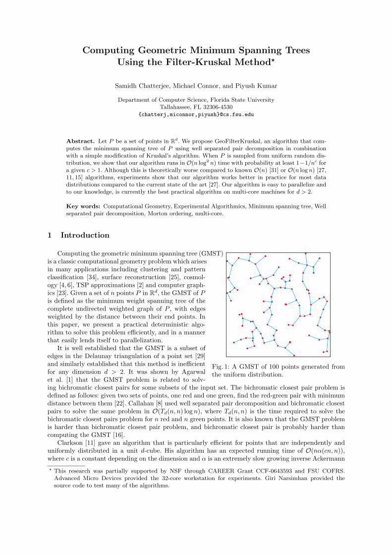
Fig. 1: A GMST of 100 points generated fromthe uniform distribution.

Computing the geometric minimum spanning tree (GMST)is a classic computational geometry problem which arisesin many applications including clustering and patternclassification [34], surface reconstruction [25], cosmol-ogy [4, 6], TSP approximations [2] and computer graph-ics [23]. Given a set of n points P in ℝd, the GMST of Pis defined as the minimum weight spanning tree of thecomplete undirected weighted graph of P , with edgesweighted by the distance between their end points. Inthis paper, we present a practical deterministic algo-rithm to solve this problem efficiently, and in a mannerthat easily lends itself to parallelization.

It is well established that the GMST is a subset ofedges in the Delaunay triangulation of a point set [29]and similarly established that this method is inefficientfor any dimension d > 2. It was shown by Agarwalet al. [1] that the GMST problem is related to solv-ing bichromatic closest pairs for some subsets of the input set. The bichromatic closest pair problem isdefined as follows: given two sets of points, one red and one green, find the red-green pair with minimumdistance between them [22]. Callahan [8] used well separated pair decomposition and bichromatic closestpairs to solve the same problem in O(Td(n, n) log n), where Td(n, n) is the time required to solve thebichromatic closest pairs problem for n red and n green points. It is also known that the GMST problemis harder than bichromatic closest pair problem, and bichromatic closest pair is probably harder thancomputing the GMST [16].

Clarkson [11] gave an algorithm that is particularly efficient for points that are independently anduniformly distributed in a unit d-cube. His algorithm has an expected running time of O(n�(cn, n)),where c is a constant depending on the dimension and � is an extremely slow growing inverse Ackermann

★ This research was partially supported by NSF through CAREER Grant CCF-0643593 and FSU COFRS.Advanced Micro Devices provided the 32-core workstation for experiments. Giri Narsimhan provided thesource code to test many of the algorithms.

function. Bentley [5] also gave an expected nearly linear time algorithm for computing GMSTs in ℝd.Dwyer [15] proved that if a set of points is generated uniformly at random from the unit ball in ℝd, itsDelaunay triangulation has linear expected complexity and can be computed in expected linear time.Since GMSTs are subsets of Euclidean Delaunay triangulations, one can combine this result with lineartime MST algorithms [20] to get an expected O(n) time algorithm for GMSTs of uniformly distributedpoints in a unit ball. Rajasekaran [31] proposed a simple expected linear time algorithm to computeGMSTs for uniform distributions in ℝd. All these approaches use bucketing techniques to execute aspiral search procedure for finding a supergraph of the GMST with O(n) edges. Unfortunately, findingk-nearest neighbors for every point, even when k =O(1) is quite an expensive operation in practice fornon-uniform distributions [32], compared to practical GMST algorithms [27, 12].

Narasimhan et al. [27] gave a practical algorithm that solves the GMST problem. They prove thatfor uniformly distributed points, in fixed dimensions, an expected O(n log n) steps suffice to computethe GMST using well separated pair decomposition. Their algorithm, GeoMST2, mimics Kruskal’s al-gorithm [21] on well separated pairs and eliminates the need to compute bichromatic closest pairs formany well separated pairs. To our knowledge, this implementation is the state of the art, for practicallycomputing GMSTs in low dimensions (d > 2). Although, improvements to GeoMST2 [27] have been an-nounced [24], exhaustive experimental results are lacking in this short announcement. Another problemwith this claim is that even for uniform distribution of points, there are no theoretical guarantees thatthe algorithm is indeed any better than O(n2).

Brennan [7] presented a modification to Kruskal’s classic minimum spanning tree (MST) algo-rithm [21] that operated similar in a manner to quicksort; splitting an edge set into “light” and “heavy”subsets. Recently, Osipov et al. [28] further expanded this idea by adding a multi-core friendly filteringstep designed to eliminate edges that were obviously not in the MST (Filter-Kruskal). Currently, thisalgorithm seems to be the most practical algorithm for computing MSTs on multi-core machines.

The algorithm presented in this paper uses well separated pair decomposition in combination witha modified version of Filter-Kruskal for computing GMSTs. We use a compressed quad-tree to build awell separated pair decomposition, followed by a sorting based algorithm similar to Filter-Kruskal. Byusing a sort based approach, we eliminate the need to maintain a priority queue [27]. This opens up thepossibility of filtering out well separated pairs with a large number of points, before it becomes necessaryto calculate their bichromatic closest pair. Additionally, we can compute the bichromatic closest pair ofwell separated pairs of similar size in batches. This allows for parallel execution of large portions of thealgorithm.

We show that our algorithm has, with high probability, a running time of O(n log2 n) on uniformlyrandom data in ℝd. Although this is a theoretically worse bound than is offered by the GeoMST2algorithm, extensive experimentation indicates that our algorithm outperforms GeoMST2 on many dis-tributions. Our theoretically worse bound comes from the fact that we have used a stricter definition ofhigh probability than being used in GeoMST2 [27]. We also present experimental results for multi-coreexecution of the algorithm.

This paper is organized as follows: In the remainder of this section, we define our notation. In Section2 we define and elaborate on tools that we use in our algorithm. Section 3 presents our algorithm, and atheoretical analysis of the running time. Section 4 describes our experimental setup, and Section 5 com-pares GeoMST2 with our algorithm experimentally. Finally, Section 6 concludes the paper and presentsfuture research directions.

Notation: Points are denoted by lower-case Roman letters. Dist(p, q) denotes the distance between thepoints p and q in L2 metric. Upper-case Roman letters are reserved for sets. Scalars except for c, d, mand n are represented by lower-case Greek letters. We reserve i, j, k for indexing purposes. Vol() denotesthe volume of an object. For a given quadtree, Box{p, q} denotes the smallest quadtree box containingpoints p and q; Fraktur letters (a) denote a quadtree node. MinDist(a, b) denotes the minimum distancebetween the quadtree boxes of two nodes. Left(a) and Right(a) denotes the left and right child of anode. ∣.∣ denotes the cardinality of a set or the number of points in a quadtree node. �(n) is used todenote inverse of the Ackermann function [13]. The Cartesian product of two sets X and Y , is denotedX × Y = {(x, y)∣x ∈ Xand y ∈ Y }.

2

2 Preliminaries

Before we present our algorithm in detail, we need to describe a few tools which our algorithm uses exten-sively. These include the well separated pair decomposition, Morton ordering and quadtree constructionthat uses this order, a practical algorithm for bichromatic closest pair computation and the union-finddata structure. We describe these tools below.

Morton ordering and Quadtrees: Morton order is a space filling curve with good locality preservingbehavior [18]. Due to this behavior, it is used in data structures for mapping multidimensional data intoone dimension. The Morton order value of a point can be obtained by interleaving the binary represen-tations of its coordinate values. If we recursively divide a d-dimensional hypercube into 2d hypercubesuntil there is only one point in each, and then order those hypercubes using their Morton order value, theMorton order curve is obtained. In 2 dimensions we refer to this decomposition as a quadtree decompo-sition, since each square can be divided into four squares. We will explain the algorithm using quadtrees,but this can be easily extended to higher dimensions. Chan [9] showed that using a few binary operationsfor integer coordinates, the relative Morton ordering can be calculated by, determining the dimension inwhich corresponding coordinates have the first differing bit in the highest bit position. This techniquecan be extended to work for floating point coordinates, with only a constant amount of extra work [12].In the next paragraph, we briefly state the quadtree construction that we use in our algorithm [10, 17].

Let p1, p2, ..., pn be a given set of points in Morton order. Let the index j be such that Vol(Box{pj−1, pj})is the largest. Then the compressed quadtreeQ for the point set consists of a root holding the Box{pj−1, pj}and two subtrees recursively built for p1, ..., pj−1 and pj , .., pn. Note that this tree is simply the Cartesiantree [17] of Vol(Box{p1, p2}), Vol(Box{p2, p3}), . . . , Vol(Box{pn−1, pn}). A Cartesian tree is a binary treeconstructed from a sequence of values which maintains three properties. First, there is one node in thetree for each value in the sequence. Second, a symmetric, in-order traversal of the tree returns the originalsequence. Finally, the tree maintains a heap property, in which a parent node has a larger value thanits child nodes. The Cartesian tree can be computed using a standard incremental algorithm in lineartime [17], given the ordering p1, p2, ..., pn [10]. Hence, for both integer as well as floating point coordinates,the compressed quadtree Q can be computed in O(n log n) [12]. We use a compressed quadtree, as op-posed to the more common fair split tree [8], because of the ease in which construction can be parallelized.

Well Separated Pair Decomposition [8]: Assume that we are given a compressed quadtree Q, builton a set of points P in ℝd. Two nodes a and b ∈ Q are said to be an �-well separated pair (�-WSP) ifthe diameter of a and the diameter of b are both at most � times the minimum distance between a andb. An �-well separated pair decomposition (�-WSPD), of size m for a quadtree Q, is a collection of wellseparated pairs of nodes {(a1, b1), ..., (am, bm)}, such that every pair of points (p, q) ∈ P ×P (p ∕= q) liesin exactly one pair (ai, bi). In the following, we use WSP and WSPD to mean well separated pairs anddecompositions with an � value of 1.

On the compressed quadtree Q, one can execute Callahan’s [8] WSPD algorithm [10]. It takes O(n)time to compute the WSPD, given the compressed quadtree, thus resulting in an overall running time ofO(n log n) for WSPD construction.

Bichromatic Closest Pair Algorithm: Given a set of points in ℝd, the Bichromatic Closest Pair(BCCP) problem asks to find the closest red-green pair [22]. The computation of the bichromatic closestpairs is necessary due to the following Lemma from [8]:

Lemma 1. The set of all the BCCP edges of the WSPD contain the edges of the GMST.

Clearly, MinDist(a, b) is the lower bound on the bichromatic closest pair distance of A and B (whereA and B are the point sets contained in a and b respectively). Next, we present the BCCP algorithm:

Algorithm 1 for computing the bichromatic closest pair was proposed by Narsimhan and Zachari-asen [27]. The input to the algorithm are two nodes a, b ∈ Q, that contain sets A,B ⊆ P and a positivereal number �, which is used by the recursive calls in the algorithm to keep track of the last closest pairdistance found. The output of the algorithm is the closest pair of points (p, q), such that p ∈ A andq ∈ B with minimum distance � = Dist(p, q). Initially, the BCCP is equal to �, where � represents theWSP containing only the last point in Morton order of A and the first point in the Morton order of B,

3

Algorithm 1 BCCP Algorithm [27]: Compute {p′, q′, �′} =Bccp(a, b[, {p, q, �} = �])

Require: a, b ∈ Q,A,B ⊆ P, � ∈ ℝ+

Require: If {p, q, �} is not specified, {p, q, �} = �, an upper bound on BCCP(a, b).1: procedure Bccp(a,b[, {p, q, �} = �])2: if (∣A∣ = 1 and ∣B∣ = 1) then3: Let p′ ∈ A, q′ ∈ B4: if Dist(p′, q′) < � then return {p′, q′, Dist(p′, q′)}5: else6: if Vol(a) < Vol(b) then Swap(a,b)7: =MinDist(Left(a), b)8: � =MinDist(Right(a), b)9: if < � then {p, q, �} =Bccp(Left(a), b, {p, q, �})

10: if � < � then {p, q, �} =Bccp(Right(a), b, {p, q, �})11: return {p, q, �}12: end procedure

assuming without loss of generality, all points in A are smaller than all points in B, in Morton order. Ifboth A and B are singleton sets, then the distance between the two points is trivially the BCCP distance.Otherwise, we compare Vol(a) and Vol(b) and compute the distance between the lighter node and eachof the children of the heavier node. If either of these distances is less than the closest pair distancecomputed so far, we recurse on the corresponding pair. If both of the distances are less, we recurse onboth of the pairs. With a slight abuse of notation, we will denote the length of the actual bichromaticclosest pair edge, between a and b, by BCCP(a,b).

UnionFind Data Structure: The UnionFind data structure maintains a set of partitions indicatingthe connectivity of points based on the edges already inserted into the GMST. Given a UnionFind datastructure G, and u, v ∈ P ⊆ ℝd, G supports the following two operations: G.Union(u, v) updates thestructure to indicate the partitions containing u and v are now joined; G.Find(u) returns the nodenumber of the representative of the partition containing u. Our implementation also does union by rankand path compression. A sequence of m G.Union() and G.Find() operations on n elements takes O(m�(n))time in the worst case. For all practical purposes, �(n) ≤ 4 (see [13]).

3 GeoFilterKruskal algorithm

Our GeoFilterKruskal algorithm computes a GMST for P ⊆ ℝd. Kruskal’s [21] algorithm shows thatgiven a set of edges, the MST can be constructed by considering edges in increasing order of weight.Using Lemma 1, the GMST can be computed by running Kruskal’s algorithm on the BCCP edges ofthe WSPD of P . When Kruskal’s algorithm adds a BCCP edge (u, v) to the GMST, where u, v ∈ P , ituses the UnionFind data structure to check whether u and v belong to the same connected component. Ifthey do, that edge is discarded. Otherwise, it is added to the GMST. Hence, before testing for an edge(u, v) for inclusion into the GMST, it should always attempt to add all BCCP edges (u′, v′) such thatDist(u′, v′) < Dist(u, v). GeoMST2 [27] avoids the computation of BCCP for many well separated pairsthat already belonged to the same connected component. Our algorithm uses this crucial observation aswell. Algorithm 2 describes the GeoFilterKruskal algorithm in more detail.

The input to the algorithm, is a WSPD of the point set P ⊆ ℝd. All procedural variables are assumedto be passed by reference. The set of WSPs S is partitioned into set El that contains WSPs withcardinality less than � (initially 2), and set Eu = S ∖El . We then compute the BCCP of all elements ofset El, and compute � equal to the minimum MinDist(a, b) for all (a, b) ∈ Eu. El is further partitionedinto El1, containing all elements with a BCCP distance less than �, and El2 = El ∖ El1. El1 is passed tothe Kruskal procedure, and El2∪Eu is passed to the Filter procedure. The Kruskal procedure addsthe edges to the GMST or discards them if they are connected. Filter removes all connected WSPs.The GeoFilterKruskal procedure is recursively called, increasing the threshold value (�) by one eachtime, on the WSPs that survive the Filter procedure, until we have constructed the minimum spanningtree.

4

Algorithm 2 GeoFilterKruskal Algorithm

Require: S = {(a1, b1), ..., (am, bm)} is a WSPD, constructed from P ⊆ ℝd ; T = {}.Ensure: BCCP Threshold � ≥ 2.1: procedure GeoFilterKruskal(Sequence of WSPs : S, Sequence of Edges : T , UnionFind : G, Integer : �)2: El = Eu = El1 = El2 = ∅3: for all (ai, bi) ∈ S do4: if (∣ai∣+ ∣bi∣) ≤ � then El = El ∪ {(ai, bi)} else Eu = Eu ∪ {(ai, bi)}5: end for6: � = min{MinDist{ai, bi} : (ai, bi) ∈ Eu, i = 1, 2, ...,m}7: for all (ai, bi) ∈ El do8: {u, v, �} = Bccp(ai, bi)9: if (� ≤ �) then El1 = El1 ∪ {(u, v)} else El2 = El2 ∪ {(u, v)}

10: end for11: Kruskal(El1, T,G)12: Enew = El2 ∪ Eu

13: Filter(Enew,G)14: if ( ∣T ∣ < (n− 1)) then GeoFilterKruskal(Enew, T,G, � + 1)15: end procedure16: procedure Kruskal(Sequence of WSPs : E, Sequence of Edges : T , UnionFind : G)17: Sort(E): by increasing BCCP distance18: for all (u, v) ∈ E do19: if G.Find(u) ∕= G.Find(v) then T = T ∪ {(u, v)} ; G.Union(u, v);20: end for21: end procedure22: procedure Filter(Sequence of WSPs : E, UnionFind : G)23: for all (ai, bi) ∈ E do24: if (G.Find(u) = G.Find(v) : u ∈ ai,v ∈ bi) then E = E ∖ {(ai, bi)}25: end for26: end procedure

3.1 Correctness

Given previous work by Kruskal [13] as well as Callahan [8], it is sufficient to show two facts to ensure thecorrectness of our algorithm. First, we are considering WSPs to be added to the GMST in the order oftheir BCCP distance. This is obviously true considering WSPs are only passed to the Kruskal procedureif their BCCP distance is less than the lower bound on the BCCP distance of the remaining WSPs. Second,we must show that the Filter procedure does not remove WSPs that should be added to the GMST.Once again, it is clear that any edge removed by the Filter procedure would have been removed by theKruskal procedure eventually, as they both use the UnionFind structure to determine connectivity.

3.2 Analysis of the running time

The real bottleneck of this algorithm, as well as the one proposed by Narasimhan [27], is the computationof the BCCP. If ∣A∣ = ∣B∣=O(n), the BCCP algorithm stated in section 3 has a worst case time complexityof O(n2). In this section we improve this bound for uniform distributions.

Let Pr(ℰ) denote the probability of occurrence of an event ℰ . In what follows, we define an eventℰ to occur with high probability (WHP) if given c > 1, Pr(ℰ) > 1 − 1/nc. Our analysis below showsthat WHP, for uniform distribution, each BCCP computation takes O(log2 n) time. Thus our wholealgorithm takes O(n log2 n) time WHP.

Let P be a set of n points chosen uniformly from a unit hypercube H in ℝd. We draw a grid of ncells in this hypercube, with the grid length being n−d, and the cell volume equal to 1/n.

Lemma 2. A quadtree box containing c log n cells contains, WHP, O(log n) points.

Proof. Let a be a quadtree box containing c log n cells. The volume of a is c log n/n. Let Xi be a randomvariable which takes the value 1 if the itℎ point of P is in a; and 0 otherwise, where i = 1, 2, ..., n. GivenPr(Xi = 1) = c log n/n and X1, ...,Xn are independent and identically distributed, let X =

∑ni=0 Xi, which

5

is binomially distributed [26] with parameters n and c log n/n. Thus the expected number of points ina box of volume c log n/n is c log n [26]. Applying Chernoff’s inequality [26], where c′ > e is a givenconstant, we see that:

Pr(X > c′ log n) < elognc′−1

/c′c′ logn = nc

′−1/nc′/ logc′ e.

Now c′/ logc′ e − (c′ − 1) > 1. Therefore, given c′ > e, Pr(X > c′ log n) < 1/n�(c′) where �(c′) > 1 is a

function of c′. Thus WHP, a quadtree containing c log n/n cells will contain O(log n) points.

Corollary 1. WHP, a quadtree box with fewer than c log n cells contains O(log n) points.

Lemma 3. Each BCCP computation takes O(log2 n) time WHP.

Proof. Let (a, b) be a WSP. Without loss of generality, assume the quadtree box a has larger volume. Ifa has � cells, then the volume of a is �/n. Since a and b are well separated, there exists a quadtree boxc with at least the same volume as a, that lies between a and b. Let ℰ denote the event that this regionis empty. Then Pr(ℰ) = (1− �/n)n ≤ 1/e�. Replacing � by c log n we have Pr(ℰ) ≤ 1/nc. Hence if a isa region containing (log n) cells, c contains one or more points with probability at least 1− 1/nc.

Note that BCCP(a, b) must be greater than BCCP(a, c) and BCCP(b, c). Since our algorithm addsthe BCCP edges by order of their increasing BCCP distance, the BCCP edge between c and a, as wellas the one between b and c, will be examined before the BCCP edge between a and b. This causes aand b to belong to the same connected component, and thus our filtering step will get rid of the wellseparated pair (a, b) before we need to compute its BCCP edge. From Lemma 2 we see that a quadtreebox containing c log n cells contains O(log n) points WHP. This fact along with Corollary 1 shows thatWHP we do not have to compute the BCCP for a quadtree box containing more than O(log n) points,limiting the run time for a BCCP calculation to O(log2 n) WHP.

Lemma 4. WHP, the total running time of the UnionFind operation is O(�(n)n log n).

Proof. From Lemma 3, WHP, all the edges in the minimum spanning tree are BCCP edges of WSPswhich are O(log n) in size. Since we increment � in steps of one, WHP, we make O(log n) calls toGeoFilterKruskal. In each of such calls, the Filter function is called once, which in turn callsthe Find(u) function of the UnionFind data structure O(n) times. Hence, there are in total O(n log n)Find(u) operations done WHP. Thus the overall running time of the Union() and Find() operations isO(�(n)n log n) WHP.

Theorem 1. Total running time of the algorithm is O(n log2 n).

Proof. We partition the list of well separated pairs twice in the GeoFilterKruskal method. The firsttime we do it based on the need to compute the BCCP of the well separated pair. We have the sets Eland Eu in the process. This takes O(n) time except for the BCCP computation. In O(n) time we canfind the pivot element of Eu for the next partition. This partitioning also takes linear time. As explainedin Lemma 4, we perform the recursive call on GeoFilterKruskal O(log n) times WHP. Thus the totaltime spent in partitioning is O(n log n) WHP. Since the total number of WSPs is O(n), the time spentin computing all such edges is O(n log2 n). Hence, the total running time of the algorithm is O(n log2 n)WHP.

Remark 1: Under the assumption that the points in P have integer coordinates, we can modify algo-rithm 2 such that its running time is O(n). WSPD can be computed in O(n) time if the coordinates ofthe points are integers [10]. One can first compute the minimum spanning forest of the k-nearest neighborgraph of the point set, for some given constant k, using a randomized linear time algorithm [19]. In thisforest, let T ′ to be the tree with the largest number of points. Rajasekaran [31] showed that there areonly n� points left to be added to T ′ to get the GMST, where � ∈ (0, 1). In our algorithm, if the set T isinitialized to T ′, then our analysis shows that WHP, only O(n� log2 n) = O(n) additional computationswill be necessary to compute the GMST.

6

Remark 2: Computation of GMST from k-nearest neighbor graph can be parallelized efficiently in aCRCW PRAM. From our analysis we can infer that in case of a uniformly randomly distributed setof points P , if we extract the O(log n) nearest neighbors for each point in the set, then these edgeswill contain the GMST of P WHP. Callahan [8] showed that it is possible to compute the k-nearestneighbors of all points in P in O(log n) time using O(kn) processors. Hence, using O(n log n) processors,the minimum spanning tree of P can then be computed in O(log n) time [33].

Remark 3: We did not pursue implementing the algorithms described in remarks one and two becausethey are inherently Monte Carlo algorithms [26]. While they can achieve a solution that is correct withhigh probability, they do not guarantee a correct solution. One can design an exact GMST algorithm us-ing k-nearest neighbor graphs; however preliminary experiments using the best practical parallel nearestneighbor codes [12, 3] showed construction times that were slower than the GeoFilterKruskal algorithm.For example, on a two dimensional data set containing one million uniformly distributed points, GeoFil-terKruskal computed the GMST in 5.5 seconds, while 8-nearest neighbor graph construction took 5.8seconds [12].

3.3 Parallelization

Parallelization of the WSPD algorithm: In our sequential version of the algorithm, each node ofthe compressed quadtree computes whether its children are well separated or not. If the children arenot well separated, we divide the larger child node, and recurse. We can parallelize this loop usingOpenMP [14] with a dynamic load balancing scheme. Since for each node there are O(1) candidates tobe well separated [10], and we are using dynamic load balancing, the total time taken in CRCW PRAM,given p processors, to execute this algorithm is O(⌈(n log n)/p⌉+ log n) including the preprocessing timefor the Morton order sort.

Parallelization of the GeoFilterKruskal algorithm: Although the whole of algorithm 2 is notparallelizable, we can parallelize most portions of the algorithm. The parallel partition algorithm [30] isused in order to divide the set S into subsets El and Eu (See Algorithm 2). � can be computed usingparallel prefix computation. In our actual implementation, we found it to be more efficient to wrap itinside the parallel partition in the previous step, using the atomic compare-and-swap instruction. Thefurther subdivision of El, as well as the Filter procedure, are just instances of parallel partition. Thesorting step used in the Kruskal procedure as well as the Morton order sort used in the construction ofthe compressed quadtree can also be parallelized [30]. We use OpenMP to do this in our implementation.Our efforts to parallelize the linear time quadtree construction showed that one can not use more numberof processors on multi-core machines to speed up this construction, because it is memory bound.

4 Experimental Setup

The GeoFilterKruskal algorithm was tested in practice against several other implementations of geometricminimum spanning tree algorithms. We chose a subset of the algorithms compared in [27], excludingsome based on the availability of source code and the clear advantage shown by some algorithms in theaforementioned work. In the experimental results section the following algorithms will be referred to:

GeoFilterKruskal was written in C++ and compiled with g++ 4.3.2 with -O3 optimization. Parallelcode was written using OpenMP [14] and the parallel mode extension to the STL [30]. C++ source code forGeoMST, GeoMST2, and Triangle were provided by Narsimhan. In addition, Triangle used Shewchuk’striangle library for Delaunay triangulation [32]. The machine used has 8 Quad-Core AMD Opteron(tm)Processor 8378 with hyperthreading enabled. Each core has a L1 cache size of 512 KB, L2 of 2MB andL3 of 6MB with 128 GB total memory. The operating system was CentOS 5.3. All data was generatedand stored as 64 bit C++ doubles.

In the next section there are two distinct series of graphs. The first set displays graphs of totalrunning time versus the number of input points, for two to five dimensional points, with uniform randomdistribution in a unit hypercube. The L2 metric was used for distances in all cases, and all algorithmswere run on the same random data set. Each algorithm was run on five data sets, and the results wereaveraged. As noted above, Triangle was not used in dimensions greater than two.

7

Table 1: Algorithm DescriptionsName Description

GeoFK# Our implementation of Algorithm 2. There are two important differences between theimplementation and the theoretical version. First, the BCCP Threshold � in section3 is incremented in steps of size O(1) instead of size 1, because this change does notaffect our analysis but helps in practice. Second, for small well separated pairs (lessthan 32 total points) the BCCP is computed by a brute force algorithm. In theexperimental results, GeoFK1 refers to the algorithm running with 1 thread. GeoFK8refers to the algorithm using 8 threads.

GeoMST Described by Callahan and Kosaraju [8]. This algorithm computes a WSPD of theinput data followed by the BCCP of every pair. It then runs Kruskal’s algorithm tofind the MST.

GeoMST2 Described in [27]. This algorithm improves on GeoMST by using marginal distancesand a priority queue to avoid many BCCP computations.

Triangle This algorithm first computes the Delaunay Triangulation of the input data, thenapplies Kruskals algorithm. Triangle was only used with two dimensional data.

The second set of graphs shows the mean total running times for two dimensional data of variousdistributions, as well as the standard deviation. The distributions were taken from [27] (given n d-dimensional points with coordinates c1...cd), shown in Table 2.

Table 2: Point Distribution InfoName Description

unif c1 to cd chosen from unit hypercube with uniform distribution (Ud)

annul c1 to c2 chosen from unit circle with uniform distribution, c3...cd chosen from Ud

arith c1 = 0, 1, 4, 9, 16... c2 to cd are 0ball c1 to cd chosen from unit hypersphere with uniform distribution

clus c1 to cd chosen from 10 clusters of normal distribution centered at 10 points chosen from Ud

edge c1 chosen from Ud, c2 to cd equal to c1diam c1 chosen from Ud, c2 to cd are 0

corn c1 to cd chosen from 2d unit hypercubes, each one centered at one of the 2d corners of a (0,2) hypercubegrid n points chosen uniformly at random from a grid with 1.3n points, the grid is housed in a unit hypercubenorm c1 to cd chosen from (−1, 1) with normal distributionspok For each dimension d′ in d n

dpoints chosen with cd′ chosen from U1 and all others equal to 1

2

5 Experimental Results

As shown in Figure 2, GeoFK1 performs favorably in practice for almost all cases compared to otheralgorithms (see Table 1). In two dimensions, only Triangle outperforms GeoFK1. In higher dimensions,GeoFK1 is the clear winner when only one thread is used. Figure 4 shows how the algorithm scales asmultiple threads are used. Eight threads were chosen as a representative for multi-core execution. We ranexperiments for points drawn from uniform random distribution, ranging from two to five dimensions.In each of these experiments, we also show how the running time of GeoFK1 varies when run on 8processors. We performed the same set of experiments for point sets from other distributions. Since thegraphs were similar to the ones for uniform distribution, they are not included.

Our algorithm tends to slowdown as the dimension increases, primarily because of the increase in thenumber of well separated pairs [27]. For example, the number of well separated pairs generated for a twodimensional uniformly distributed data set of size 106 was approximately 107, whereas a five dimensionaldata set of the same size had 108 WSPs.

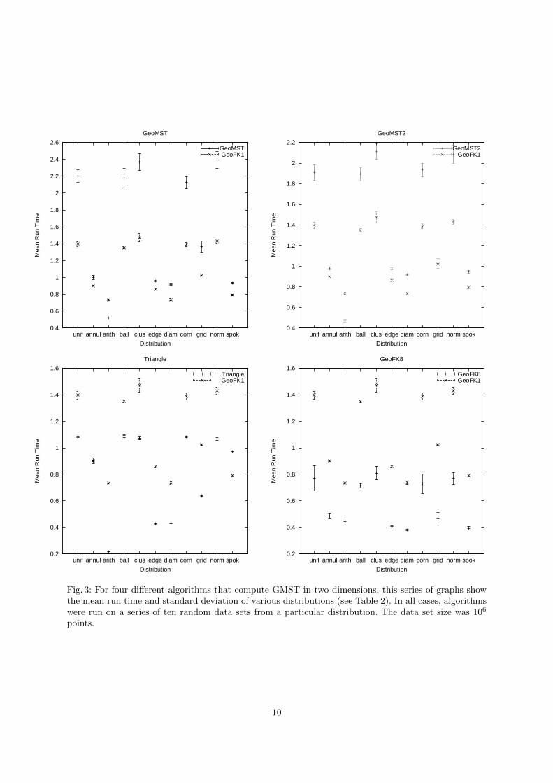
Figure 3 shows that in most cases, GeoFK1 performs better regardless of the distribution of theinput point set. Apart from the fact that Triangle maintains its superiority in two dimensions, GeoFK1performs better in all the distributions that we have considered, except when the points are drawn from

8

aritℎ distribution. In the data set from aritℎ, the ordering of the WSPs based on the minimum distanceis the same as based on the BCCP distance. Hence the second partitioning step in GeoFK1 acts as anoverhead. The results from Figure 3 are for two dimensional data. The same experiments for data setsof other dimensions did not give significantly different results, and so were not included.

0

20

40

60

80

100

120

140

160

180

200

10987654321

Tot

al R

un T

ime

Number of Points/106

2-d

GeoMSTGeoMST2GeoFK1GeoFK8Triangle

0

5

10

15

20

25

30

35

40

45

50

10987654321

Tot

al R

un T

ime

Number of Points/105

3-d

GeoMSTGeoMST2GeoFK1GeoFK8

0

50

100

150

200

250

10987654321

Tot

al R

un T

ime

Number of Points/105

4-d

GeoMSTGeoMST2GeoFK1GeoFK8

0

200

400

600

800

1000

1200

10987654321

Tot

al R

un T

ime

Number of Points/105

5-d

GeoMSTGeoMST2GeoFK1GeoFK8

Fig. 2: This series of graphs shows the total running time for each algorithm for varying sized data setsof uniformly random points, as the dimension increases. Data sets ranged from 106 to 107 points for2-d data, and 105 to 106 for other dimensions. For each data set size 5 tests were done and the resultsaveraged.

9

0.4

0.6

0.8

1

1.2

1.4

1.6

1.8

2

2.2

2.4

2.6

spoknormgridcorndiamedgeclusballarithannulunif

Mea

n R

un T

ime

Distribution

GeoMST

GeoMSTGeoFK1

0.4

0.6

0.8

1

1.2

1.4

1.6

1.8

2

2.2

spoknormgridcorndiamedgeclusballarithannulunif

Mea

n R

un T

ime

Distribution

GeoMST2

GeoMST2GeoFK1

0.2

0.4

0.6

0.8

1

1.2

1.4

1.6

spoknormgridcorndiamedgeclusballarithannulunif

Mea

n R

un T

ime

Distribution

Triangle

TriangleGeoFK1

0.2

0.4

0.6

0.8

1

1.2

1.4

1.6

spoknormgridcorndiamedgeclusballarithannulunif

Mea

n R

un T

ime

Distribution

GeoFK8

GeoFK8GeoFK1

Fig. 3: For four different algorithms that compute GMST in two dimensions, this series of graphs showthe mean run time and standard deviation of various distributions (see Table 2). In all cases, algorithmswere run on a series of ten random data sets from a particular distribution. The data set size was 106

points.

10

2

3

4

5

6

7

8

9

0 10 20 30 40 50 60 70

Tot

al R

un T

ime

Number of Threads

Multi-core scaling of GeoFK

AMDIntel

Fig. 4: This figure demonstrates the run time gains of the algorithm as more threads are used. We presentscaling for two architectures. The AMD line was computed on the machine described in Section 4. TheIntel line used a machine with four 2.66GHz Intel(R) Xeon(R) CPU X5355, 4096 KB of L1 cache, and8GB total memory. All cases were run on 20 data sets from uniform random distribution of size 106

points, final total run time is an average of the results.

6 Conclusions and Future Work

This paper strives to demonstrate a practical GMST algorithm, that is theoretically efficient on uniformlydistributed point sets, works well on most distributions and is multi-core friendly. To that effect weintroduced the GeoFilterKruskal algorithm, an efficient, parallelizable GMST algorithm that in boththeory and practice accomplished our goals. We proved a running time of O(n log2 n) with a strictdefinition of high probability, as well as showed extensive experimental results.

This work raises many interesting open problems. Since the main parallel portions of the algorithmrely on partitioning and sorting, the practical impact of other parallel sort and partition algorithmsshould be explored. In addition, since the particular well separated pair decomposition algorithm used isnot relevant to the correctness of our algorithm, the use of a tree that offers better clustering might makethe algorithm more efficient. Experiments were conducted only for L2 metric in this paper. As a part ofour future work, we plan to perform experiments on other metrics. We also plan to do more extensiveexperiments on the k-nearest neighbor approach in higher dimensions, for example d > 10.

References

1. Pankaj K. Agarwal, Herbert Edelsbrunner, Otfried Schwarzkopf, and Emo Welzl. Euclidean minimum span-ning trees and bichromatic closest pairs. Discrete Comput. Geom., 6(5):407–422, 1991.

2. Sanjeev Arora. Polynomial time approximation schemes for euclidean traveling salesman and other geometricproblems. J. ACM, 45(5):753–782, 1998.

3. Sunil Arya, David M. Mount, Nathan S. Netanyahu, Ruth Silverman, and Angela Y. Wu. An optimalalgorithm for approximate nearest neighbor searching fixed dimensions. J. ACM, 45(6):891–923, 1998.

4. J.D. Barrow, S.P. Bhavsar, and D.H. Sonoda. Min-imal spanning trees, filaments and galaxy clustering.MNRAS, 216:17–35, Sept 1985.

5. Jon Louis Bentley, Bruce W. Weide, and Andrew C. Yao. Optimal expected-time algorithms for closest pointproblems. ACM Trans. Math. Softw., 6(4):563–580, 1980.

11

6. S. P. Bhavsar and R. J. Splinter. The superiority of the minimal spanning tree in percolation analyses ofcosmological data sets. MNRAS, 282:1461–1466, Oct 1996.

7. J.J. Brennan. Minimal spanning trees and partial sorting. Operations Research Letters, 1(3):138–141, 1982.8. Paul B. Callahan. Dealing with higher dimensions: the well-separated pair decomposition and its applications.

PhD thesis, Johns Hopkins University, Baltimore, MD, USA, 1995.9. Timothy M. Chan. Manuscript: A minimalist’s implementation of an approximate nearest n eighbor algorithm

in fixed dimensions, 2006.10. Timothy M. Chan. Well-separated pair decomposition in linear time? Inf. Process. Lett., 107(5):138–141,

2008.11. Kenneth L. Clarkson. An algorithm for geometric minimum spanning trees requiring nearly linear expected

time. Algorithmica, 4:461–469, 1989. Included in PhD Thesis.12. Michael Connor and Piyush Kumar. Parallel construction of k-nearest neighbor graphs for point clouds. In

Proceedings of Volume and Point-Based Graphics., pages 25–32. IEEE VGTC, August 2008.13. Thomas H. Cormen, Charles E. Leiserson, Ronald L. Rivest, and Clifford Stein. Introduction to Algorithms.

MIT Press and McGraw-Hill, 2001.14. L. Dagum and R. Menon. Openmp: an industry standard api for shared-memory programming. IEEE

Computational Science and Engineering, 5(1):46–55, 1998.15. R. A. Dwyer. Higher-dimensional voronoi diagrams in linear expected time. In SCG ’89: Proceedings of the

fifth annual symposium on Computational geometry, pages 326–333, New York, NY, USA, 1989. ACM.16. Jeff Erickson. On the relative complexities of some geometric problems. In In Proc. 7th Canad. Conf.

Comput. Geom, pages 85–90, 1995.17. Harold N. Gabow, Jon Louis Bentley, and Robert E. Tarjan. Scaling and related techniques for geometry

problems. In STOC ’84: Proceedings of the sixteenth annual ACM symposium on Theory of computing, pages135–143, New York, NY, USA, 1984. ACM.

18. G.M.Morton. A computer oriented geodetic data base; and a new technique in file sequencing. Technicalreport, IBM Ltd., Ottawa, Canada, 1966.

19. David R. Karger, Philip N. Klein, and Robert E. Tarjan. A randomized linear-time algorithm to find minimumspanning trees. Journal of the ACM, 42:321–328, 1995.

20. Philip N. Klein and Robert E. Tarjan. A randomized linear-time algorithm for finding minimum spanningtrees. In STOC ’94: Proceedings of the twenty-sixth annual ACM symposium on Theory of computing, pages9–15, New York, NY, USA, 1994. ACM.

21. J.B. Kruskal. On the shortest spanning subtree of a graph and the traveling salesman problem. In Proc.American Math. Society, pages 7–48, 1956.

22. Drago Krznaric, Christos Levcopoulos, and Bengt J. Nilsson. Minimum spanning trees in d dimensions.Nordic J. of Computing, 6(4):446–461, 1999.

23. Elmar Langetepe and Gabriel Zachmann. Geometric Data Structures for Computer Graphics. A. K. Peters,Ltd., Natick, MA, USA, 2006.

24. W. March and A. Gray. Large-scale euclidean mst and hierarchical clustering. Workshop on Efficient MachineLearning, 2007.

25. Robert Mencl. A graph based approach to surface reconstruction. Computer Graphics Forum, 14:445 – 456,2008.

26. Michael Mitzenmacher and Eli Upfal. Probability and Computing: Randomized Algorithms and ProbabilisticAnalysis. Cambridge University Press, New York, NY, USA, 2005.

27. Giri Narasimhan and Martin Zachariasen. Geometric minimum spanning trees via well-separated pair de-compositions. J. Exp. Algorithmics, 6:6, 2001.

28. Vitaly Osipov, Peter Sanders, and Johannes Singler. The filter-kruskal minimum spanning tree algorithm.In Irene Finocchi and John Hershberger, editors, ALENEX, pages 52–61. SIAM, 2009.

29. Franco P. Preparata and Michael I. Shamos. Computational geometry: an introduction. Springer-Verlag NewYork, Inc., New York, NY, USA, 1985.

30. Felix Putze, Peter Sanders, and Johannes Singler. Mcstl: the multi-core standard template library. In PPoPP’07: Proceedings of the 12th ACM SIGPLAN symposium on Principles and practice of parallel programming,pages 144–145, New York, NY, USA, 2007. ACM.

31. Sanguthevar Rajasekaran. On the euclidean minimum spanning tree problem. Computing Letters, 1(1), 2004.32. Jonathan Richard Shewchuk. Triangle: Engineering a 2D Quality Mesh Generator and Delaunay Triangu-

lator. In Ming C. Lin and Dinesh Manocha, editors, Applied Computational Geometry: Towards GeometricEngineering, volume 1148 of Lecture Notes in Computer Science, pages 203–222. Springer-Verlag, May 1996.From the First ACM Workshop on Applied Computational Geometry.

33. Francis Suraweera and Prabir Bhattacharya. An o(log m) parallel algorithm for the minimum spanning treeproblem. Inf. Process. Lett., 45(3):159–163, 1993.

34. C.T. Zahn. Graph-theoretical methods for detecting and describing gestalt clusters. Transactions on Com-puters, C-20(1):68–86, 1971.

12