Computing Game-Theoretic Solutions

Vincent ConitzerDuke University

overview article: V. Conitzer. Computing Game-Theoretic Solutions and Applications to Security. Proc. AAAI’12.

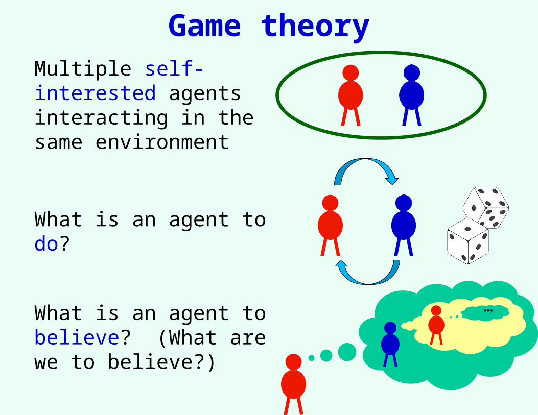
Game theoryMultiple self-interested agents interacting in the same environment

What is an agent to do?

What is an agent to believe? (What are we to believe?)

…

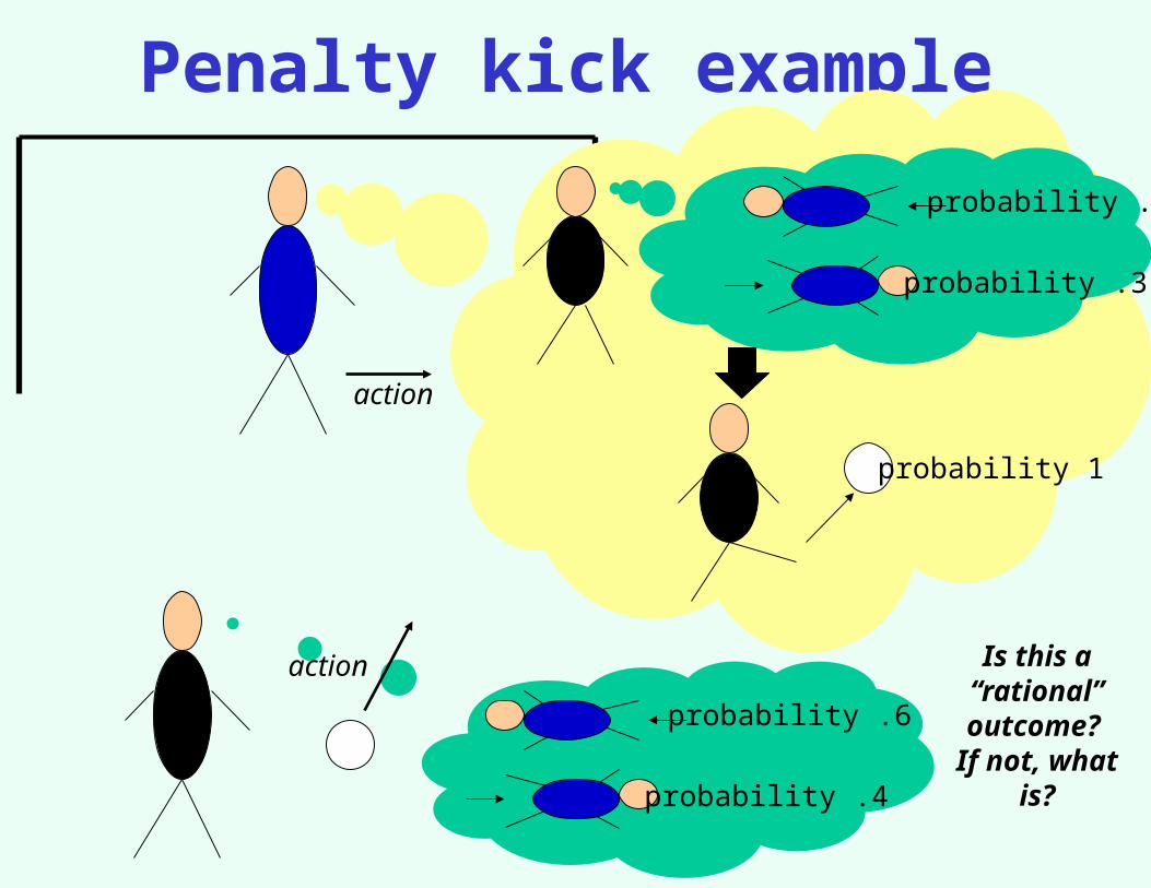
Penalty kick example

probability .7

probability .3

probability .6

probability .4

probability 1

Is this a “rational” outcome? If not, what

is?

action

action

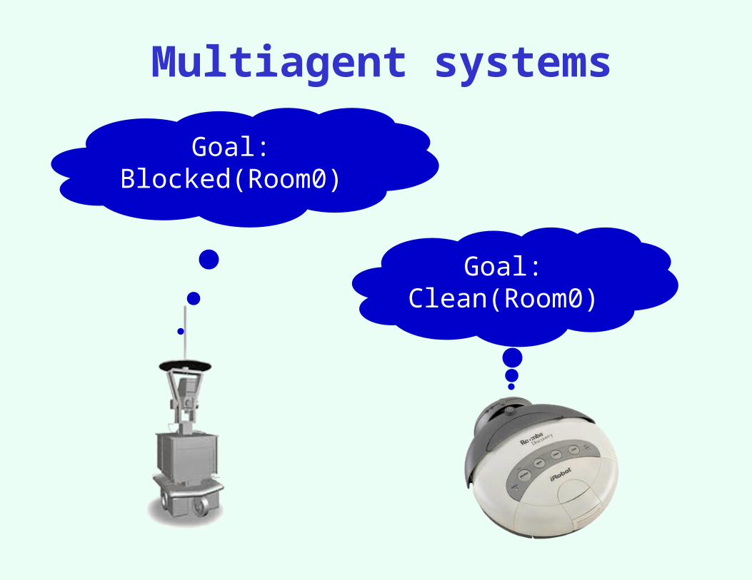
Multiagent systems

Goal: Blocked(Room0)

Goal: Clean(Room0)

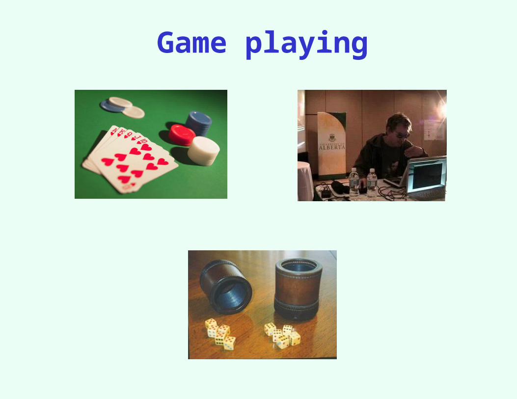
Game playing

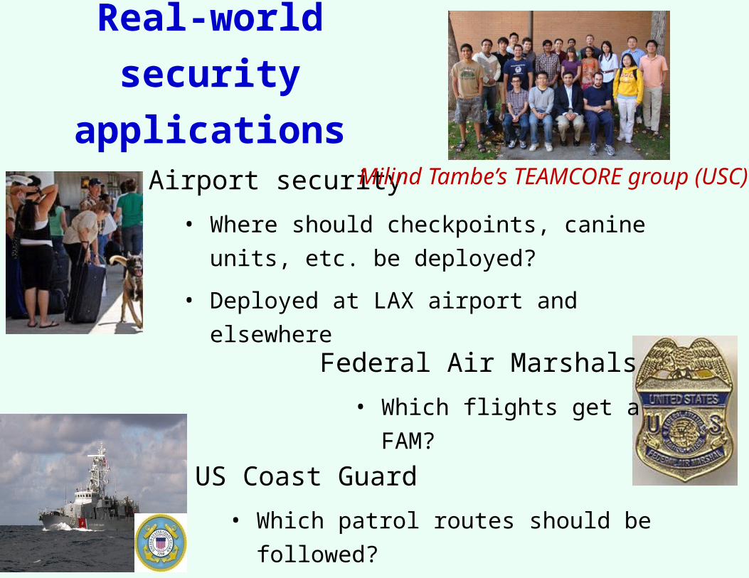
Real-world security

applications

Airport security

• Where should checkpoints, canine units,

etc. be deployed?

• Deployed at LAX airport and elsewhere

US Coast Guard

• Which patrol routes should be followed?

• Deployed in Boston, New York, Los Angeles

Federal Air Marshals

• Which flights get a FAM?

Milind Tambe’s TEAMCORE group (USC)

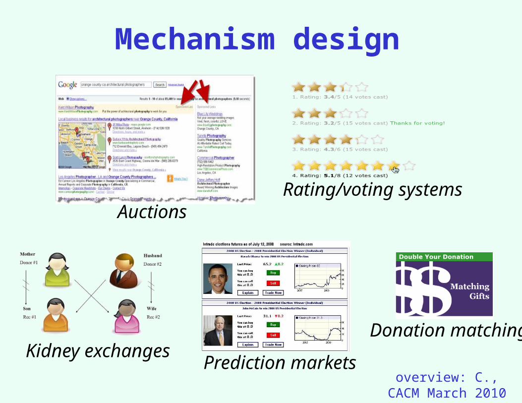
Mechanism design

Auctions

Kidney exchangesPrediction markets

Rating/voting systems

Donation matching

overview: C., CACM March 2010

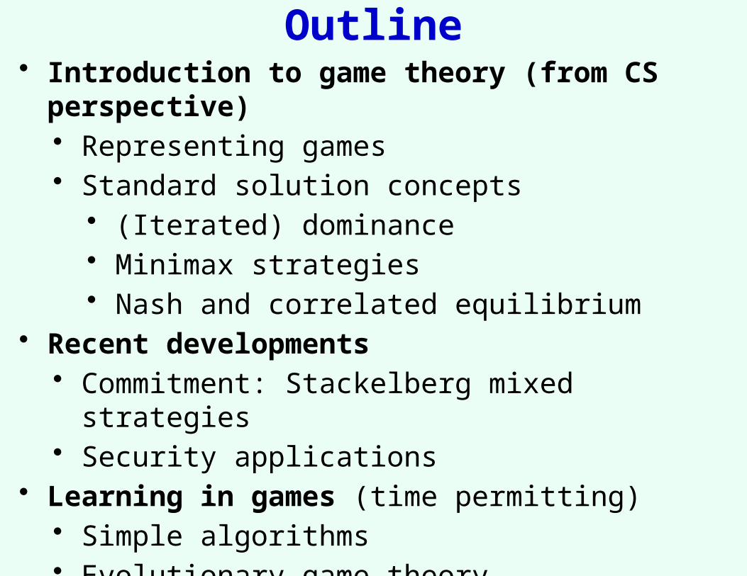
Outline• Introduction to game theory (from CS perspective)

• Representing games• Standard solution concepts

• (Iterated) dominance• Minimax strategies• Nash and correlated equilibrium

• Recent developments• Commitment: Stackelberg mixed strategies• Security applications

• Learning in games (time permitting)• Simple algorithms• Evolutionary game theory• Learning in Stackelberg games

Representing games

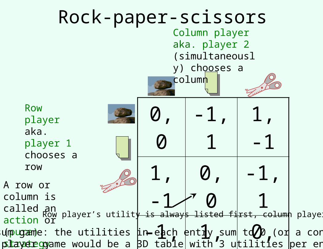
Rock-paper-scissors

0, 0 -1, 1 1, -1

1, -1 0, 0 -1, 1

-1, 1 1, -1 0, 0

Row player aka. player 1 chooses a row

Column player aka. player 2 (simultaneously) chooses a column

A row or column is called an action or (pure) strategy

Row player’s utility is always listed first, column player’s second

Zero-sum game: the utilities in each entry sum to 0 (or a constant)Three-player game would be a 3D table with 3 utilities per entry, etc.

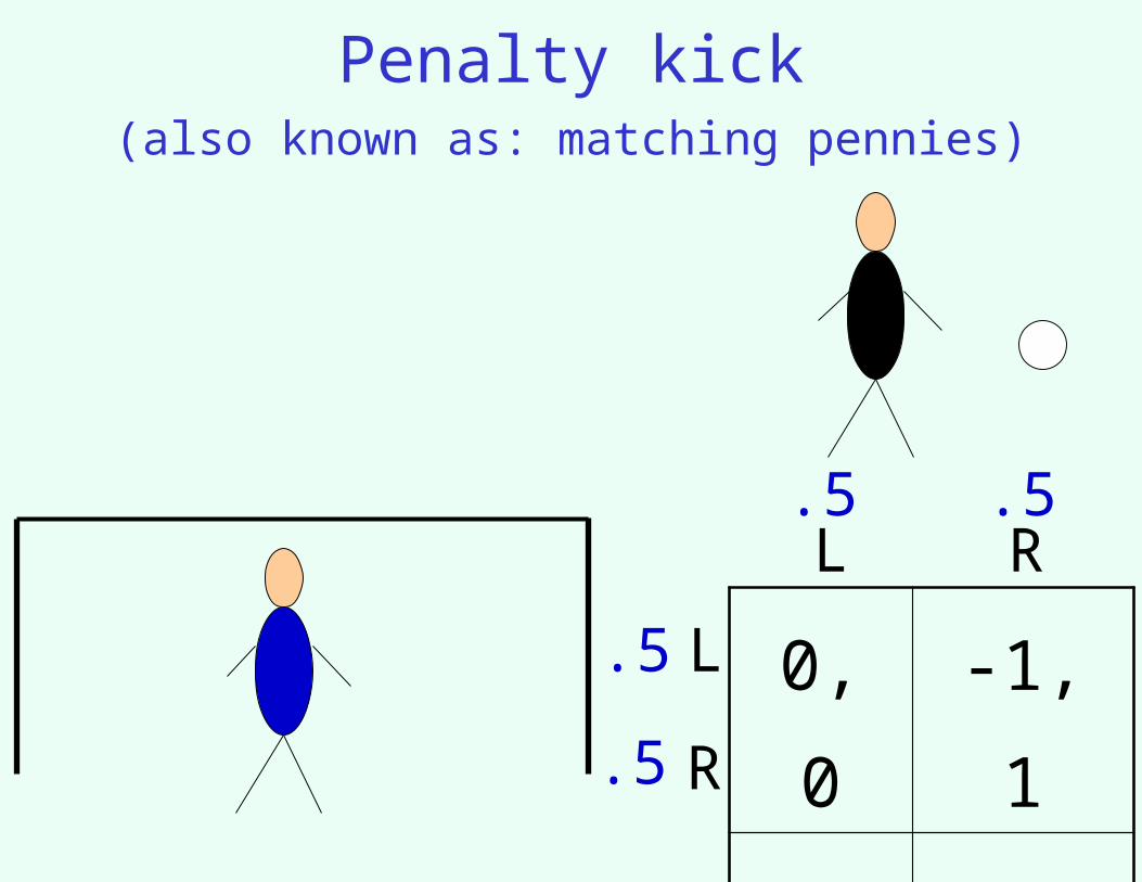
Penalty kick(also known as: matching pennies)

0, 0 -1, 1

-1, 1 0, 0

L

R

L R

.5

.5

.5 .5

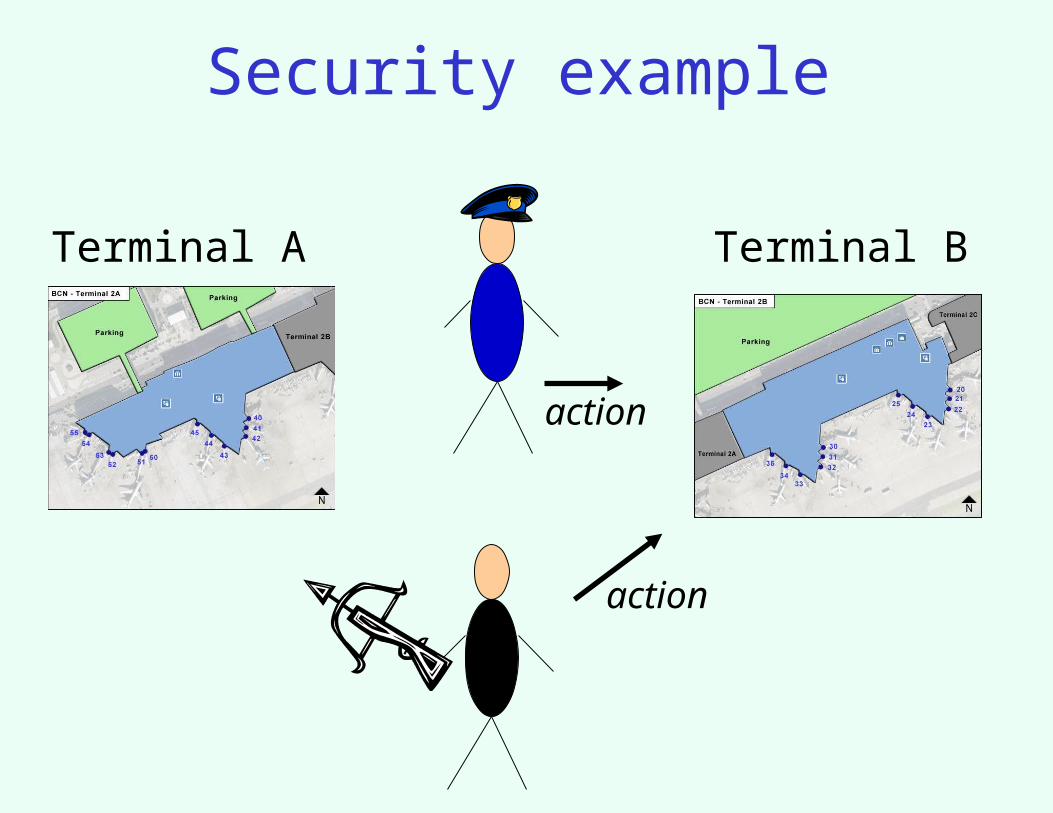
Security example

action

action

Terminal A Terminal B

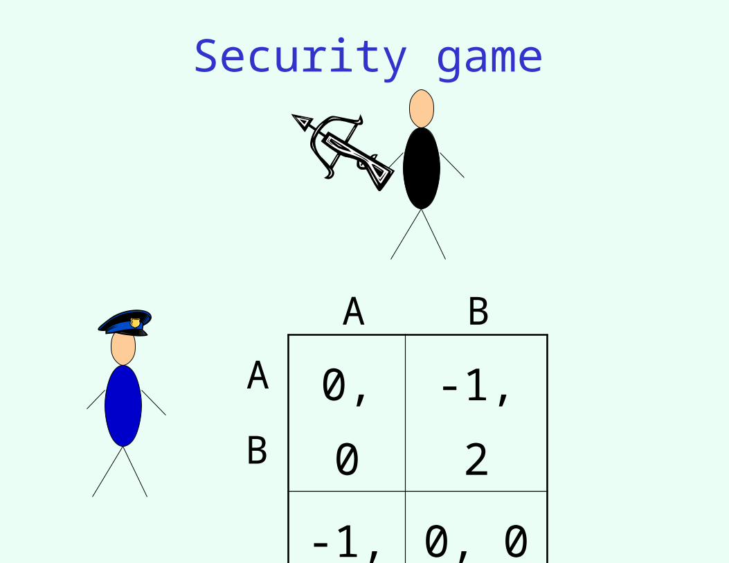
Security game

0, 0 -1, 2

-1, 1 0, 0

A

B

A B

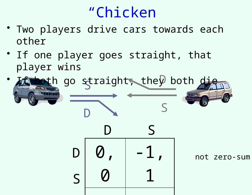
“Chicken”

0, 0 -1, 1

1, -1 -5, -5D

S

D S

S

D

D

S

• Two players drive cars towards each other• If one player goes straight, that player wins• If both go straight, they both die

not zero-sum

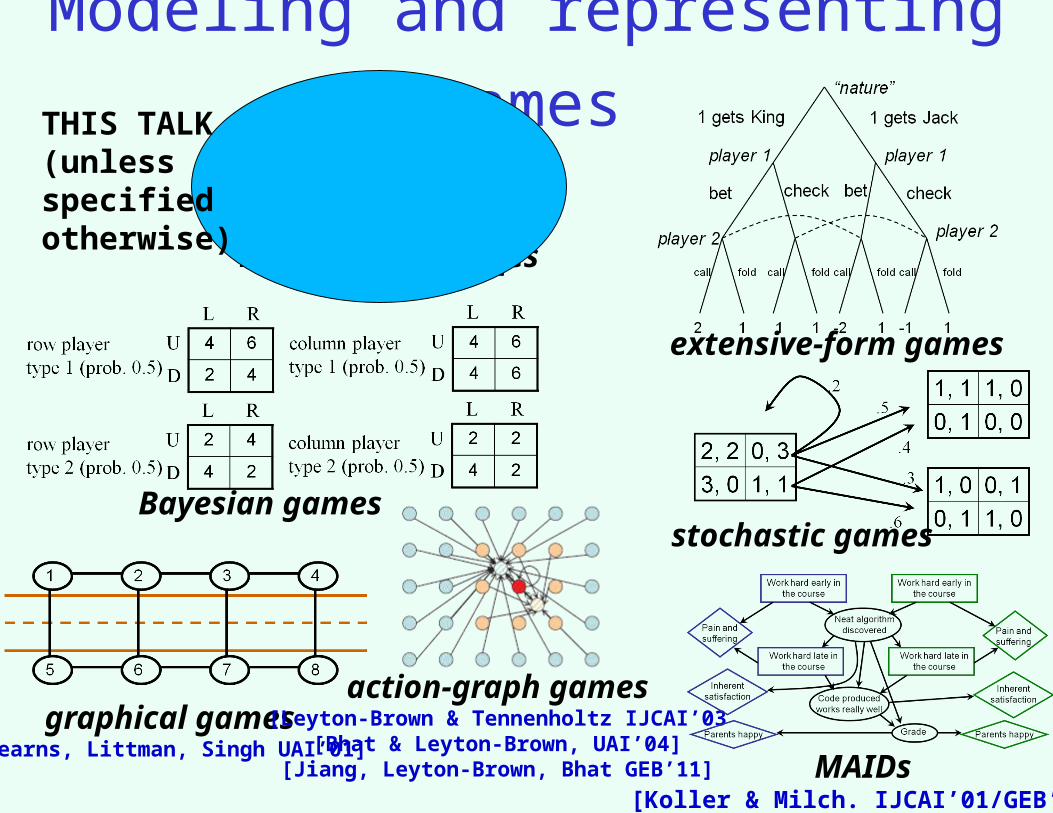
Modeling and representing games2, 2 -1, 0

-7, -8 0, 0

normal-form games

extensive-form games

Bayesian gamesstochastic games

graphical games[Kearns, Littman, Singh UAI’01]

action-graph games[Leyton-Brown & Tennenholtz IJCAI’03

[Bhat & Leyton-Brown, UAI’04][Jiang, Leyton-Brown, Bhat GEB’11] MAIDs

[Koller & Milch. IJCAI’01/GEB’03]

THIS TALK(unless specified otherwise)

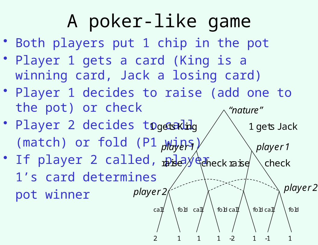
A poker-like game• Both players put 1 chip in the pot• Player 1 gets a card (King is a winning card, Jack a

losing card)• Player 1 decides to raise (add one to the pot) or

check• Player 2 decides to call

(match) or fold (P1 wins)• If player 2 called, player

1’s card determines

pot winner

1 gets King 1 gets Jack

raise raisecheck check

call fold call fold call fold call fold

“nature”

player 1player 1

player 2 player 2

2 1 1 1 -2 -11 1

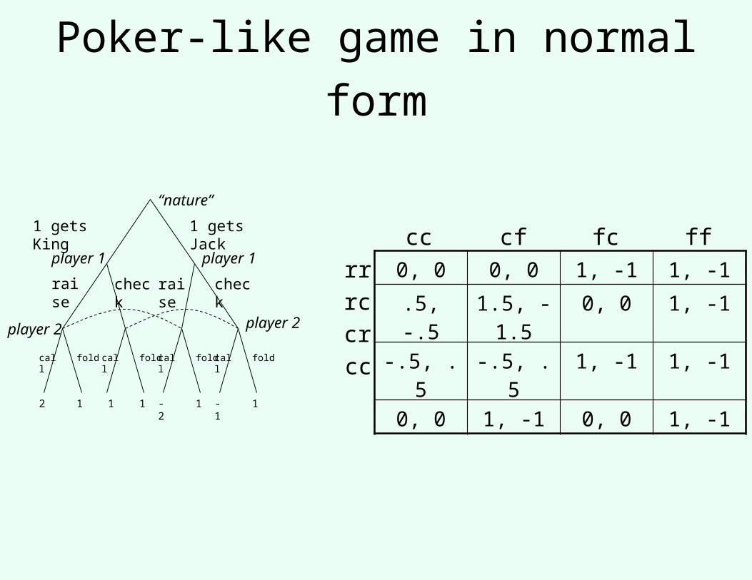
Poker-like game in normal form

1 gets King 1 gets Jack

raise raisecheck check

call fold call fold call fold call fold

“nature”

player 1player 1

player 2 player 2

2 1 1 1 -2 -11 1

0, 0 0, 0 1, -1 1, -1

.5, -.5 1.5, -1.5 0, 0 1, -1

-.5, .5 -.5, .5 1, -1 1, -1

0, 0 1, -1 0, 0 1, -1

cc cf fc ff

rr

cr

cc

rc

Our first solution concept: Dominance

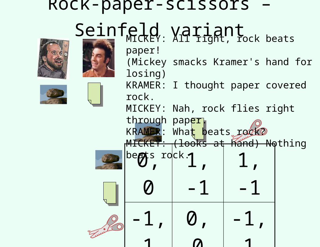
Rock-paper-scissors – Seinfeld variant

0, 0 1, -1 1, -1

-1, 1 0, 0 -1, 1

-1, 1 1, -1 0, 0

MICKEY: All right, rock beats paper!(Mickey smacks Kramer's hand for losing)KRAMER: I thought paper covered rock.MICKEY: Nah, rock flies right through paper.KRAMER: What beats rock?MICKEY: (looks at hand) Nothing beats rock.

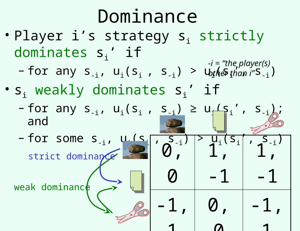
Dominance• Player i’s strategy si strictly dominates si’ if

– for any s-i, ui(si , s-i) > ui(si’, s-i)

• si weakly dominates si’ if – for any s-i, ui(si , s-i) ≥ ui(si’, s-i); and– for some s-i, ui(si , s-i) > ui(si’, s-i)

0, 0 1, -1 1, -1

-1, 1 0, 0 -1, 1

-1, 1 1, -1 0, 0

strict dominance

weak dominance

-i = “the player(s) other than i”

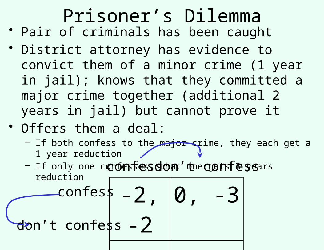
Prisoner’s Dilemma

-2, -2 0, -3

-3, 0 -1, -1

confess

• Pair of criminals has been caught• District attorney has evidence to convict them of a

minor crime (1 year in jail); knows that they committed a major crime together (additional 2 years in jail) but cannot prove it

• Offers them a deal:– If both confess to the major crime, they each get a 1 year reduction– If only one confesses, that one gets 3 years reduction

don’t confess

don’t confess

confess

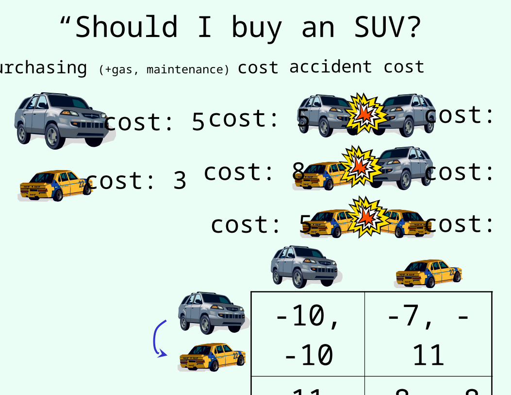
“Should I buy an SUV?”

-10, -10 -7, -11

-11, -7 -8, -8

cost: 5

cost: 3

cost: 5 cost: 5

cost: 5 cost: 5

cost: 8 cost: 2

purchasing (+gas, maintenance) cost accident cost

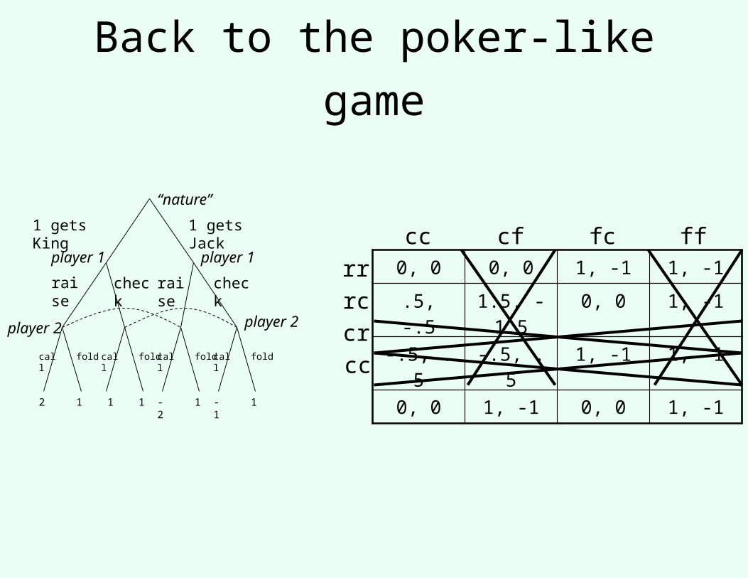
Back to the poker-like game

1 gets King 1 gets Jack

raise raisecheck check

call fold call fold call fold call fold

“nature”

player 1player 1

player 2 player 2

2 1 1 1 -2 -11 1

0, 0 0, 0 1, -1 1, -1

.5, -.5 1.5, -1.5 0, 0 1, -1

-.5, .5 -.5, .5 1, -1 1, -1

0, 0 1, -1 0, 0 1, -1

cc cf fc ff

rr

cr

cc

rc

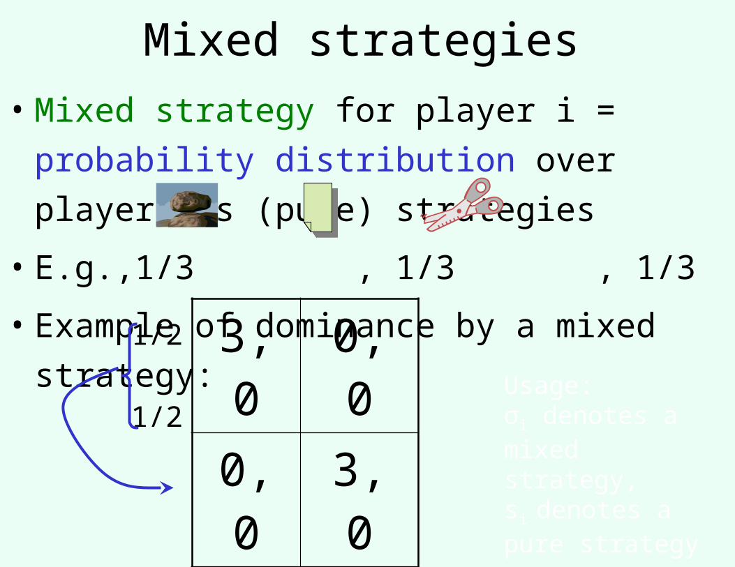
Mixed strategies

• Mixed strategy for player i = probability

distribution over player i’s (pure) strategies

• E.g.,1/3 , 1/3 , 1/3

• Example of dominance by a mixed strategy:

3, 0 0, 0

0, 0 3, 0

1, 0 1, 0

1/2

1/2Usage: σi denotes a mixed strategy, si denotes a pure strategy

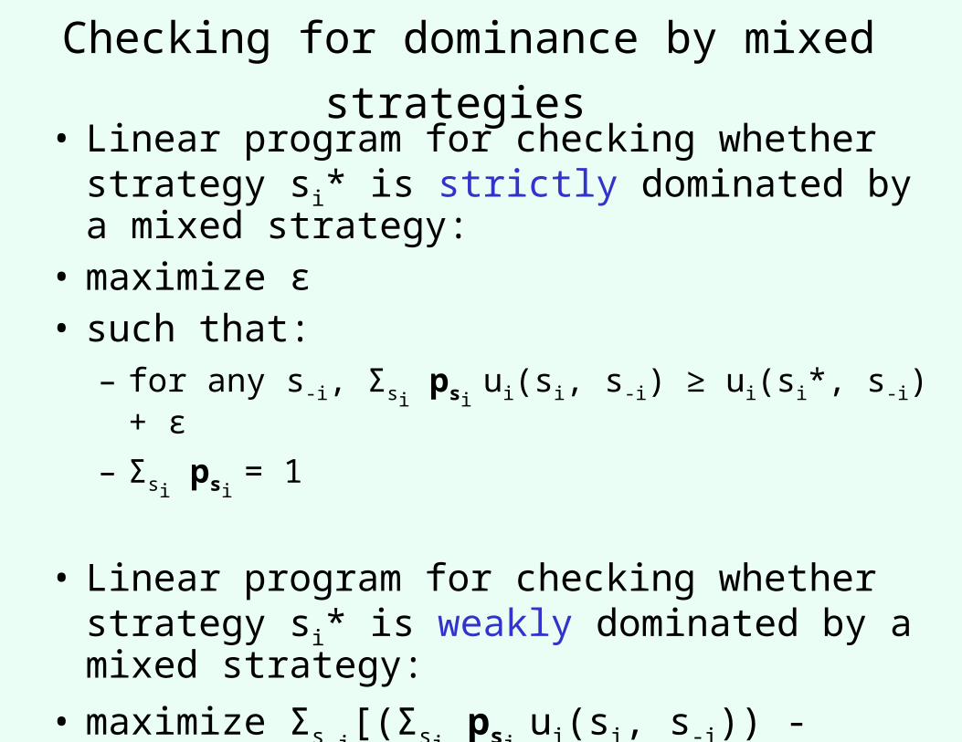
Checking for dominance by mixed strategies

• Linear program for checking whether strategy si* is strictly dominated by a mixed strategy:

• maximize ε• such that:

– for any s-i, Σsi psi

ui(si, s-i) ≥ ui(si*, s-i) + ε

– Σsi psi

= 1

• Linear program for checking whether strategy si* is weakly dominated by a mixed strategy:

• maximize Σs-i[(Σsi

psi ui(si, s-i)) - ui(si*, s-i)]

• such that: – for any s-i, Σsi

psi ui(si, s-i) ≥ ui(si*, s-i)

– Σsi psi

= 1

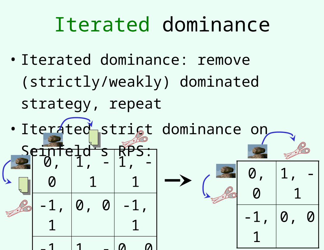
Iterated dominance

• Iterated dominance: remove (strictly/weakly)

dominated strategy, repeat

• Iterated strict dominance on Seinfeld’s RPS:

0, 0 1, -1 1, -1

-1, 1 0, 0 -1, 1

-1, 1 1, -1 0, 0

0, 0 1, -1

-1, 1 0, 0

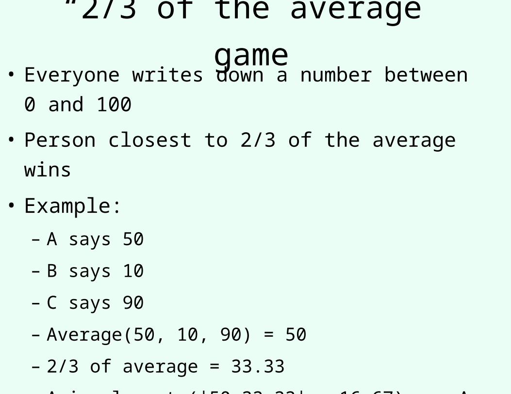
“2/3 of the average” game• Everyone writes down a number between 0 and 100

• Person closest to 2/3 of the average wins

• Example:

– A says 50

– B says 10

– C says 90

– Average(50, 10, 90) = 50

– 2/3 of average = 33.33

– A is closest (|50-33.33| = 16.67), so A wins

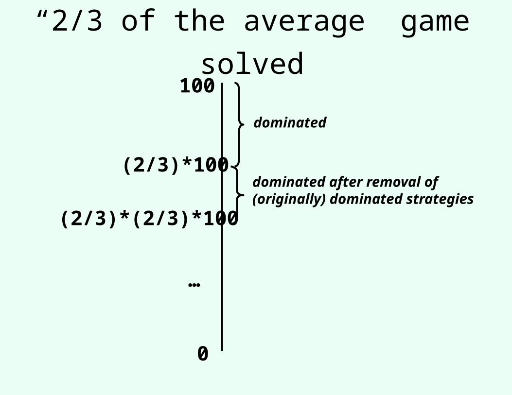
“2/3 of the average” game solved

0

100

(2/3)*100

(2/3)*(2/3)*100

…

dominated

dominated after removal of (originally) dominated strategies

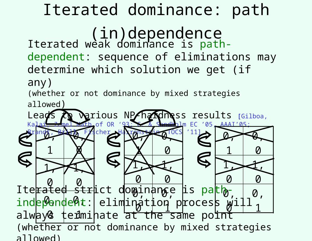
Iterated dominance: path (in)dependence

0, 1 0, 0

1, 0 1, 0

0, 0 0, 1

Iterated weak dominance is path-dependent: sequence of eliminations may determine which solution we get (if any)(whether or not dominance by mixed strategies allowed)Leads to various NP-hardness results [Gilboa, Kalai, Zemel Math of OR ‘93; C. & Sandholm EC ’05, AAAI’05; Brandt, Brill, Fischer, Harrenstein TOCS ’11]

0, 1 0, 0

1, 0 1, 0

0, 0 0, 1

0, 1 0, 0

1, 0 1, 0

0, 0 0, 1

Iterated strict dominance is path-independent: elimination process will always terminate at the same point(whether or not dominance by mixed strategies allowed)

Solving two-player zero-sum games

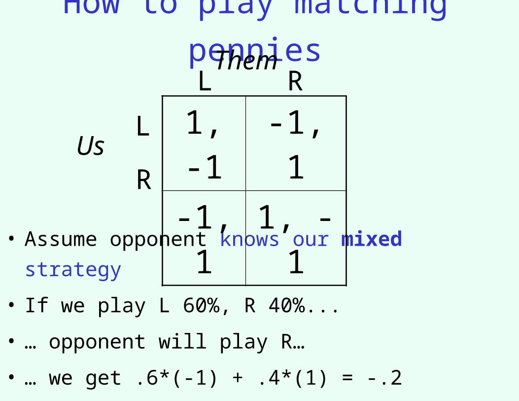
How to play matching pennies

• Assume opponent knows our mixed strategy

• If we play L 60%, R 40%...

• … opponent will play R…

• … we get .6*(-1) + .4*(1) = -.2

• What’s optimal for us? What about rock-paper-scissors?

1, -1 -1, 1

-1, 1 1, -1L

R

L R

Us

Them

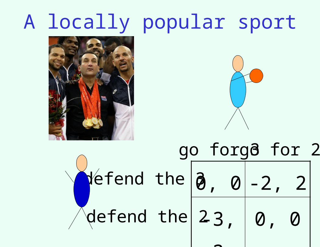
A locally popular sport

0, 0 -2, 2

-3, 3 0, 0

defend the 3

defend the 2

go for 3 go for 2

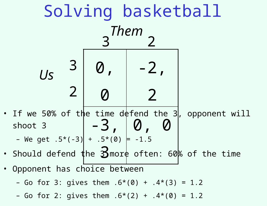
Solving basketball

• If we 50% of the time defend the 3, opponent will shoot 3

– We get .5*(-3) + .5*(0) = -1.5

• Should defend the 3 more often: 60% of the time

• Opponent has choice between

– Go for 3: gives them .6*(0) + .4*(3) = 1.2

– Go for 2: gives them .6*(2) + .4*(0) = 1.2

• We get -1.2 (the maximin value)

0, 0 -2, 2

-3, 3 0, 0

3

2

3 2

Us

Them

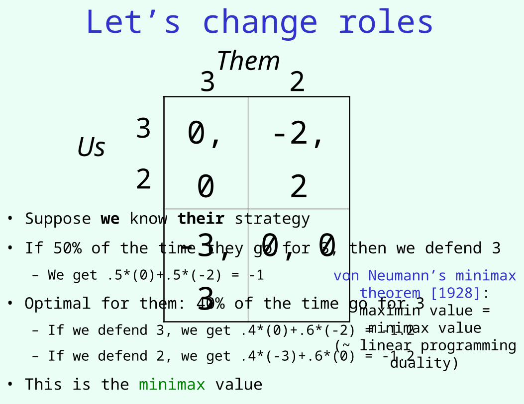
Let’s change roles

• Suppose we know their strategy

• If 50% of the time they go for 3, then we defend 3

– We get .5*(0)+.5*(-2) = -1

• Optimal for them: 40% of the time go for 3

– If we defend 3, we get .4*(0)+.6*(-2) = -1.2

– If we defend 2, we get .4*(-3)+.6*(0) = -1.2

• This is the minimax value

0, 0 -2, 2

-3, 3 0, 0

3

2

3 2

Us

Them

von Neumann’s minimax theorem [1928]: maximin value = minimax value

(~ linear programming duality)

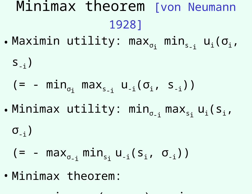
Minimax theorem [von Neumann 1928]

• Maximin utility: maxσi mins-i

ui(σi, s-i)

(= - minσi maxs-i

u-i(σi, s-i))

• Minimax utility: minσ-i maxsi

ui(si, σ-i)

(= - maxσ-i minsi

u-i(si, σ-i))

• Minimax theorem:

maxσi mins-i

ui(σi, s-i) = minσ-i maxsi

ui(si, σ-i)

• Minimax theorem does not hold with pure

strategies only (example?)

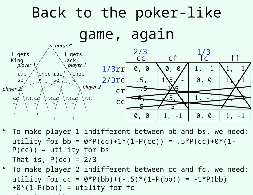
Back to the poker-like game, again

1 gets King 1 gets Jack

raise raisecheck check

call fold call fold call fold call fold

“nature”

player 1player 1

player 2 player 2

2 1 1 1 -2 -11 1

0, 0 0, 0 1, -1 1, -1

.5, -.5 1.5, -1.5 0, 0 1, -1

-.5, .5 -.5, .5 1, -1 1, -1

0, 0 1, -1 0, 0 1, -1

cc cf fc ff

rr

cr

cc

rc

2/3 1/3

1/3

2/3

• To make player 1 indifferent between bb and bs, we need:

utility for bb = 0*P(cc)+1*(1-P(cc)) = .5*P(cc)+0*(1-P(cc)) = utility for bs

That is, P(cc) = 2/3• To make player 2 indifferent between cc and fc, we need:

utility for cc = 0*P(bb)+(-.5)*(1-P(bb)) = -1*P(bb)+0*(1-P(bb)) = utility for fc

That is, P(bb) = 1/3

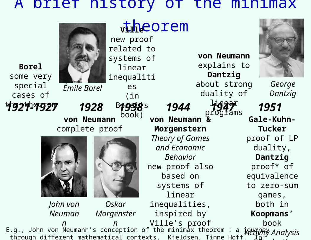
A brief history of the minimax theorem

Borelsome very

special cases of the theorem

1921-1927 1928von Neumanncomplete proof

1938

Villenew proof related to

systems of linear

inequalities(in Borel’s

book)

1944von Neumann &

MorgensternTheory of Games

and Economic Behavior

new proof also based on systems of linear inequalities, inspired

by Ville’s proof

von Neumannexplains to

Dantzig about strong duality of linear programs

1947Gale-Kuhn-

Tuckerproof of LP duality,

Dantzigproof* of

equivalence to zero-sum games,

both in Koopmans’ bookActivity Analysis

of Production and Allocation

1951

John von Neumann

Émile Borel

Oskar Morgenstern

George Dantzig

E.g., John von Neumann's conception of the minimax theorem : a journey through different mathematical contexts. Kjeldsen, Tinne Hoff. In: Archive for History of Exact Sciences, Vol. 56, 2001, p. 39-68.

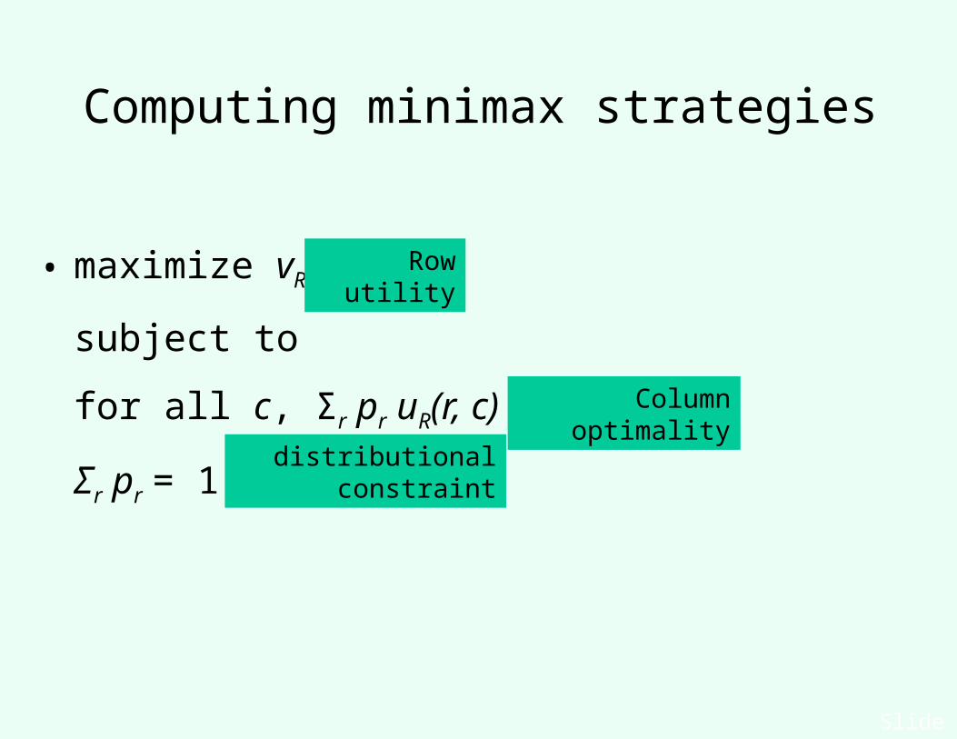
Computing minimax strategies

• maximize vR

subject to

for all c, Σr pr uR(r, c) ≥ vR

Σr pr = 1

Slide 7

Row utility

distributional constraint

Column optimality

Equilibrium notions for general-sum games

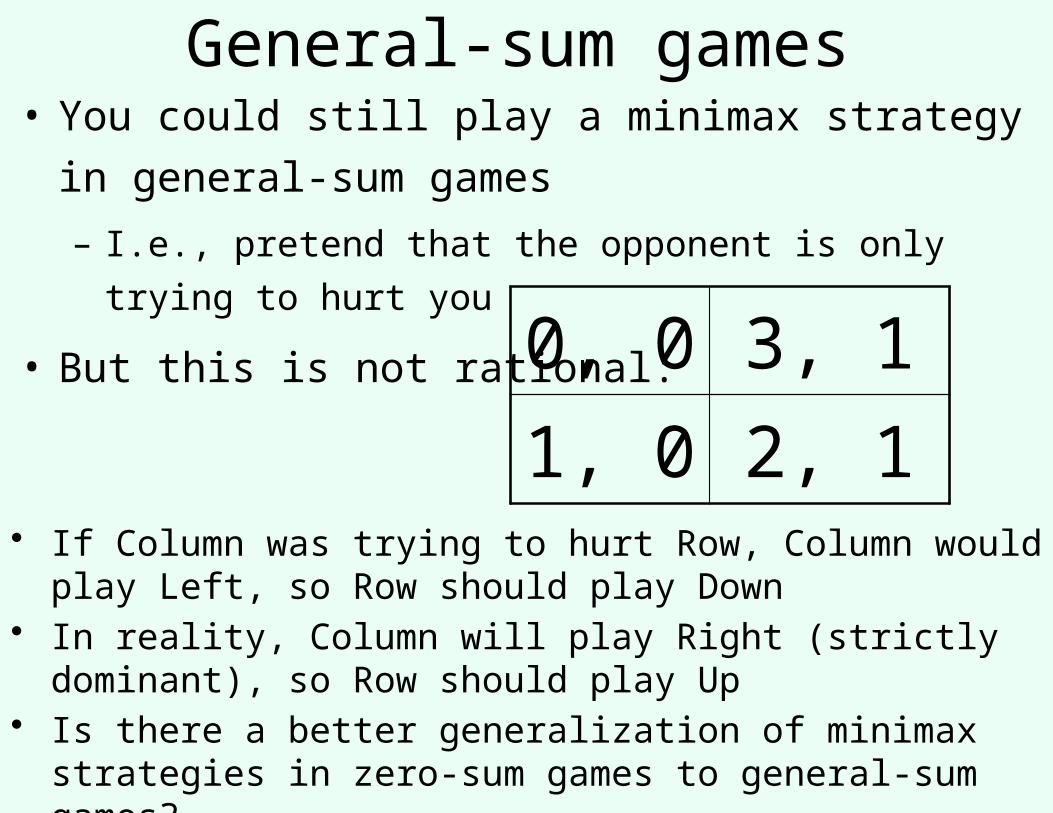
General-sum games• You could still play a minimax strategy in general-sum

games

– I.e., pretend that the opponent is only trying to hurt you

• But this is not rational: 0, 0 3, 11, 0 2, 1

• If Column was trying to hurt Row, Column would play Left, so Row should play Down

• In reality, Column will play Right (strictly dominant), so Row should play Up

• Is there a better generalization of minimax strategies in zero-sum games to general-sum games?

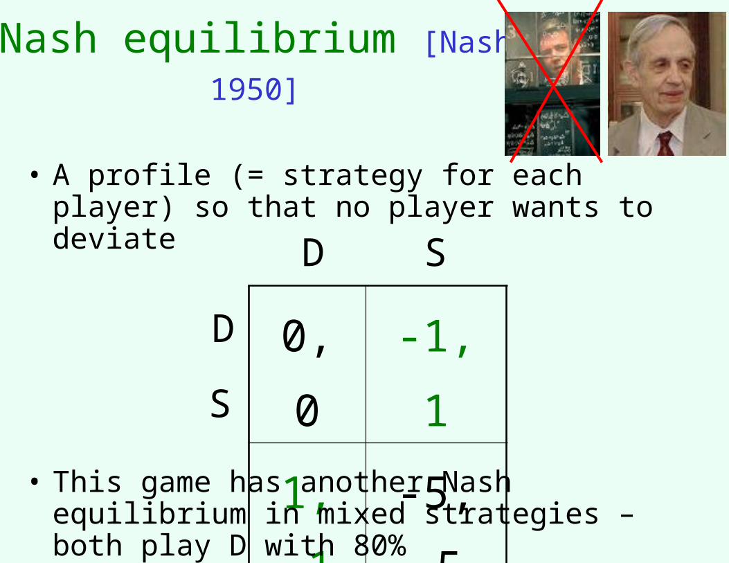
Nash equilibrium [Nash 1950]

• A profile (= strategy for each player) so that no player wants to deviate

0, 0 -1, 1

1, -1 -5, -5

D

S

D S

• This game has another Nash equilibrium in mixed strategies – both play D with 80%

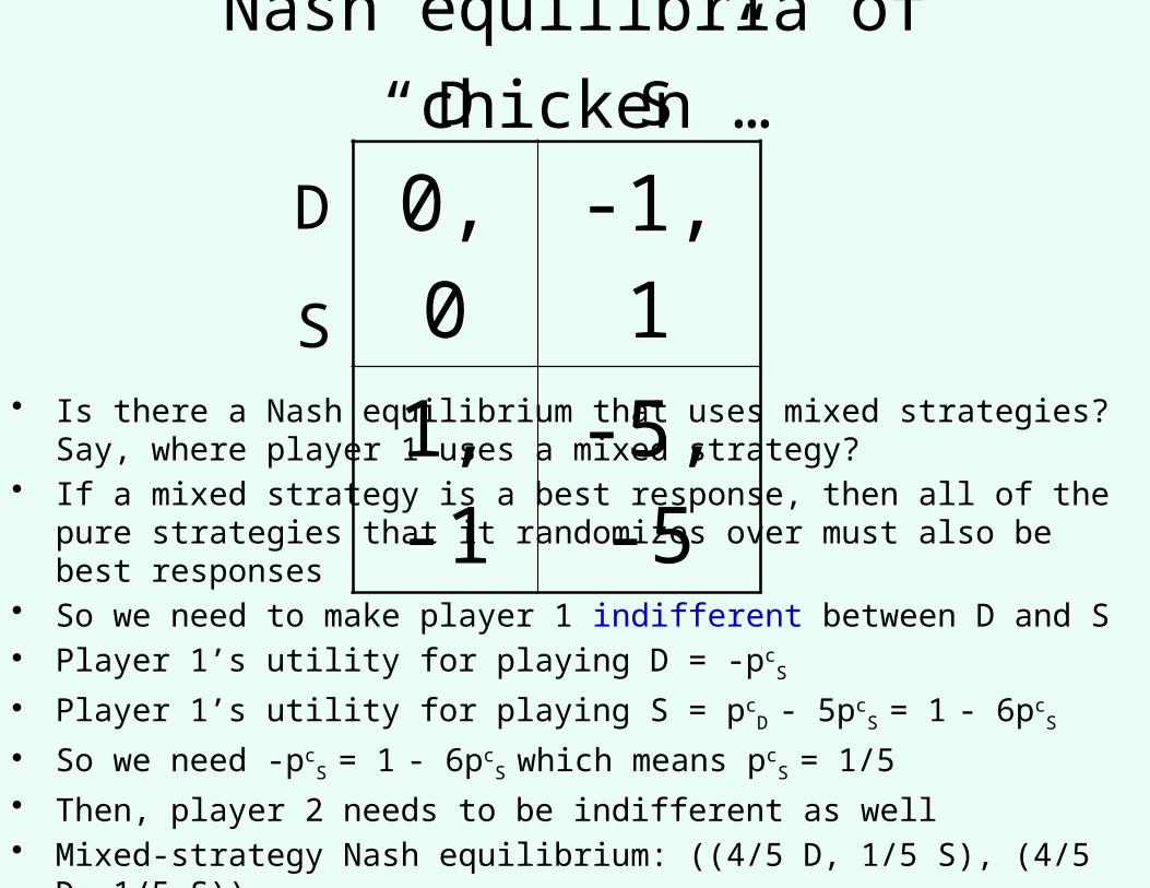
Nash equilibria of “chicken”…

0, 0 -1, 1

1, -1 -5, -5D

S

D S

• Is there a Nash equilibrium that uses mixed strategies? Say, where player 1 uses a mixed strategy?

• If a mixed strategy is a best response, then all of the pure strategies that it randomizes over must also be best responses

• So we need to make player 1 indifferent between D and S• Player 1’s utility for playing D = -pc

S

• Player 1’s utility for playing S = pcD - 5pc

S = 1 - 6pcS

• So we need -pcS = 1 - 6pc

S which means pcS = 1/5

• Then, player 2 needs to be indifferent as well• Mixed-strategy Nash equilibrium: ((4/5 D, 1/5 S), (4/5 D, 1/5 S))

– People may die! Expected utility -1/5 for each player

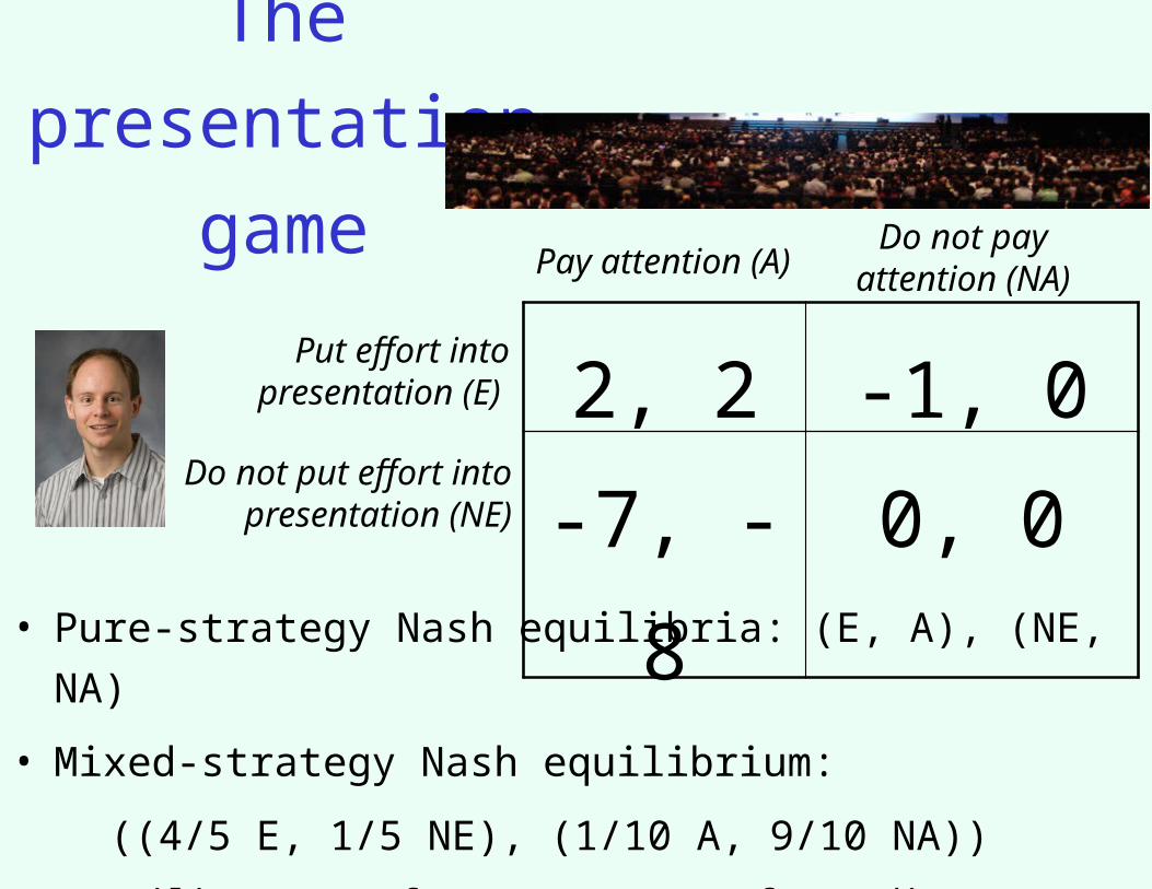
The presentation

gamePay attention (A)

Do not pay attention (NA)

Put effort into presentation (E)

Do not put effort into presentation (NE)

2, 2 -1, 0

-7, -8 0, 0

• Pure-strategy Nash equilibria: (E, A), (NE, NA)

• Mixed-strategy Nash equilibrium:

((4/5 E, 1/5 NE), (1/10 A, 9/10 NA))

– Utility -7/10 for presenter, 0 for audience

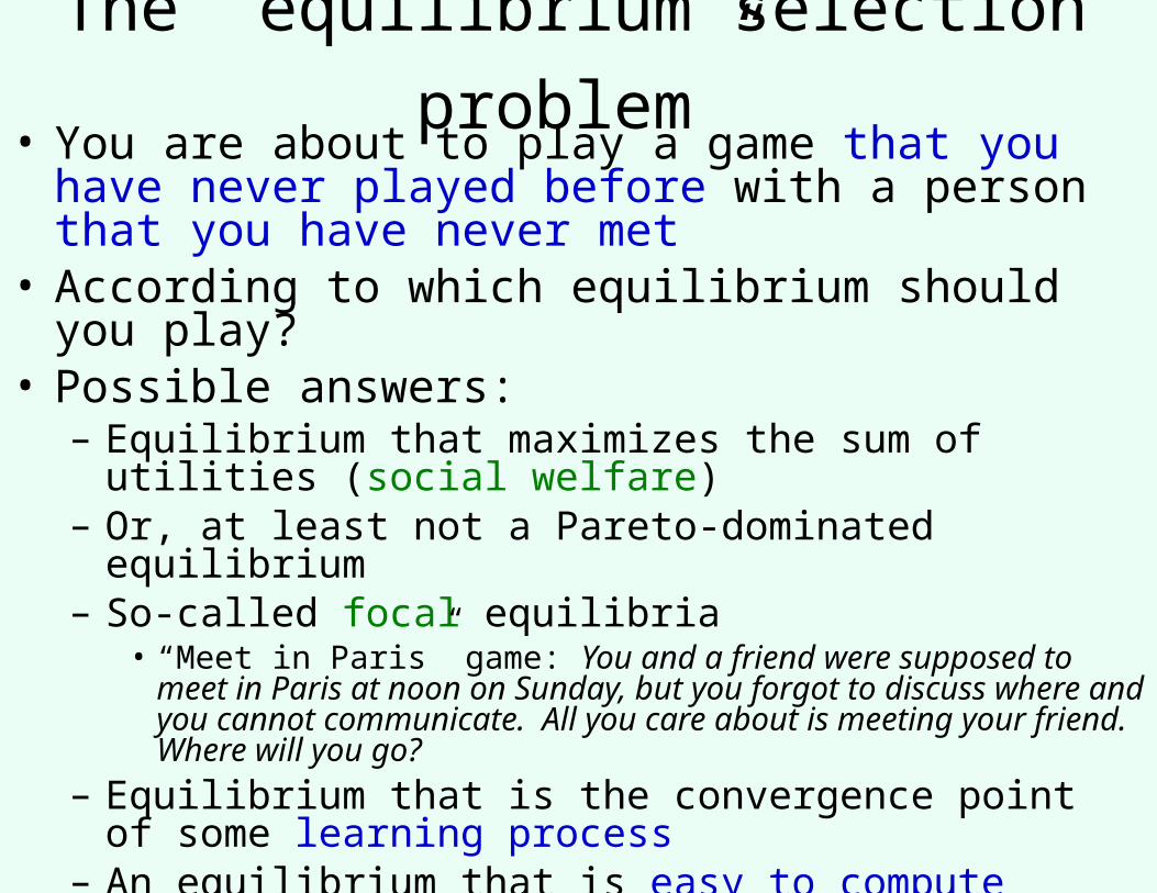
The “equilibrium selection problem”• You are about to play a game that you have never

played before with a person that you have never met• According to which equilibrium should you play?• Possible answers:

– Equilibrium that maximizes the sum of utilities (social welfare)

– Or, at least not a Pareto-dominated equilibrium– So-called focal equilibria

• “Meet in Paris” game: You and a friend were supposed to meet in Paris at noon on Sunday, but you forgot to discuss where and you cannot communicate. All you care about is meeting your friend. Where will you go?

– Equilibrium that is the convergence point of some learning process

– An equilibrium that is easy to compute– …

• Equilibrium selection is a difficult problem

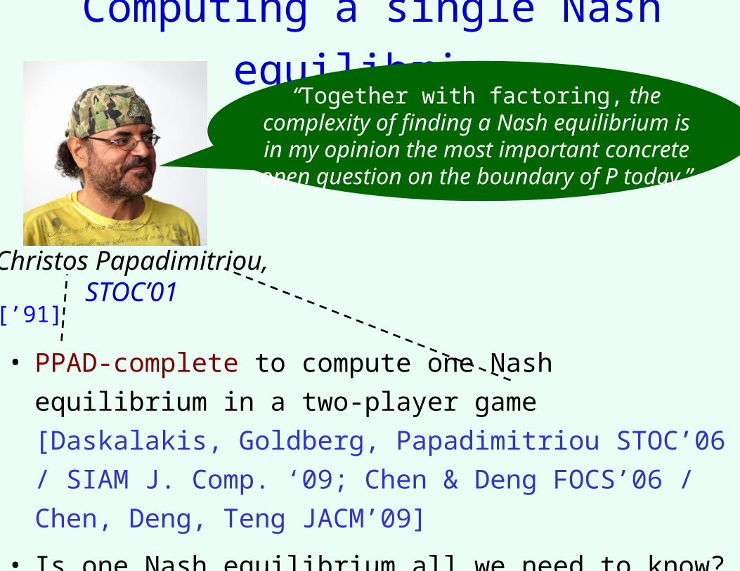
Computing a single Nash equilibrium

• PPAD-complete to compute one Nash equilibrium in a two-

player game [Daskalakis, Goldberg, Papadimitriou STOC’06

/ SIAM J. Comp. ‘09; Chen & Deng FOCS’06 / Chen, Deng,

Teng JACM’09]

• Is one Nash equilibrium all we need to know?

“Together with factoring, the complexity of finding a Nash equilibrium is in my opinion the most important concrete open question

on the boundary of P today.”

Christos Papadimitriou, STOC’01

[’91]

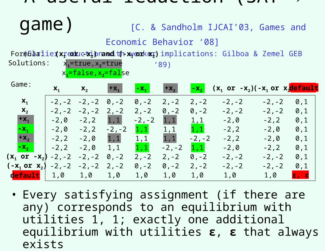
A useful reduction (SAT → game) [C. & Sandholm IJCAI’03, Games and Economic Behavior ‘08]

(Earlier reduction with weaker implications: Gilboa & Zemel GEB ‘89)Formula: (x1 or -x2) and (-x1 or x2)Solutions: x1=true,x2=true

x1=false,x2=false

Game: x1 x2 +x1 -x1 +x2 -x2 (x1 or -x2) (-x1 or x2) default

x1 -2,-2 -2,-2 0,-2 0,-2 2,-2 2,-2 -2,-2 -2,-2 0,1x2 -2,-2 -2,-2 2,-2 2,-2 0,-2 0,-2 -2,-2 -2,-2 0,1

+x1 -2,0 -2,2 1,1 -2,-2 1,1 1,1 -2,0 -2,2 0,1-x1 -2,0 -2,2 -2,-2 1,1 1,1 1,1 -2,2 -2,0 0,1+x2 -2,2 -2,0 1,1 1,1 1,1 -2,-2 -2,2 -2,0 0,1-x2 -2,2 -2,0 1,1 1,1 -2,-2 1,1 -2,0 -2,2 0,1

(x1 or -x2) -2,-2 -2,-2 0,-2 2,-2 2,-2 0,-2 -2,-2 -2,-2 0,1(-x1 or x2) -2,-2 -2,-2 2,-2 0,-2 0,-2 2,-2 -2,-2 -2,-2 0,1default 1,0 1,0 1,0 1,0 1,0 1,0 1,0 1,0 ε, ε

• Every satisfying assignment (if there are any) corresponds to an equilibrium with utilities 1, 1; exactly one additional equilibrium with utilities ε, ε that always exists

• Evolutionarily stable strategies Σ2P-complete [C. WINE 2013]

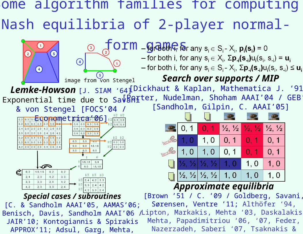
Some algorithm families for computing Nash

equilibria of 2-player normal-form games

Lemke-Howson [J. SIAM ‘64]Exponential time due to Savani & von Stengel [FOCS’04 / Econometrica’06]

Search over supports / MIP[Dickhaut & Kaplan, Mathematica J. ‘91]

[Porter, Nudelman, Shoham AAAI’04 / GEB’08][Sandholm, Gilpin, C. AAAI’05]

Special cases / subroutines[C. & Sandholm AAAI’05, AAMAS’06; Benisch,

Davis, Sandholm AAAI’06 / JAIR’10; Kontogiannis & Spirakis APPROX’11; Adsul,

Garg, Mehta, Sohoni STOC’11; …]

Approximate equilibria[Brown ’51 / C. ’09 / Goldberg, Savani, Sørensen,

Ventre ’11; Althöfer ‘94, Lipton, Markakis, Mehta ‘03, Daskalakis, Mehta, Papadimitriou ‘06, ‘07, Feder, Nazerzadeh, Saberi ‘07, Tsaknakis & Spirakis ‘07,

Spirakis ‘08, Bosse, Byrka, Markakis ‘07, …]

image from von Stengel

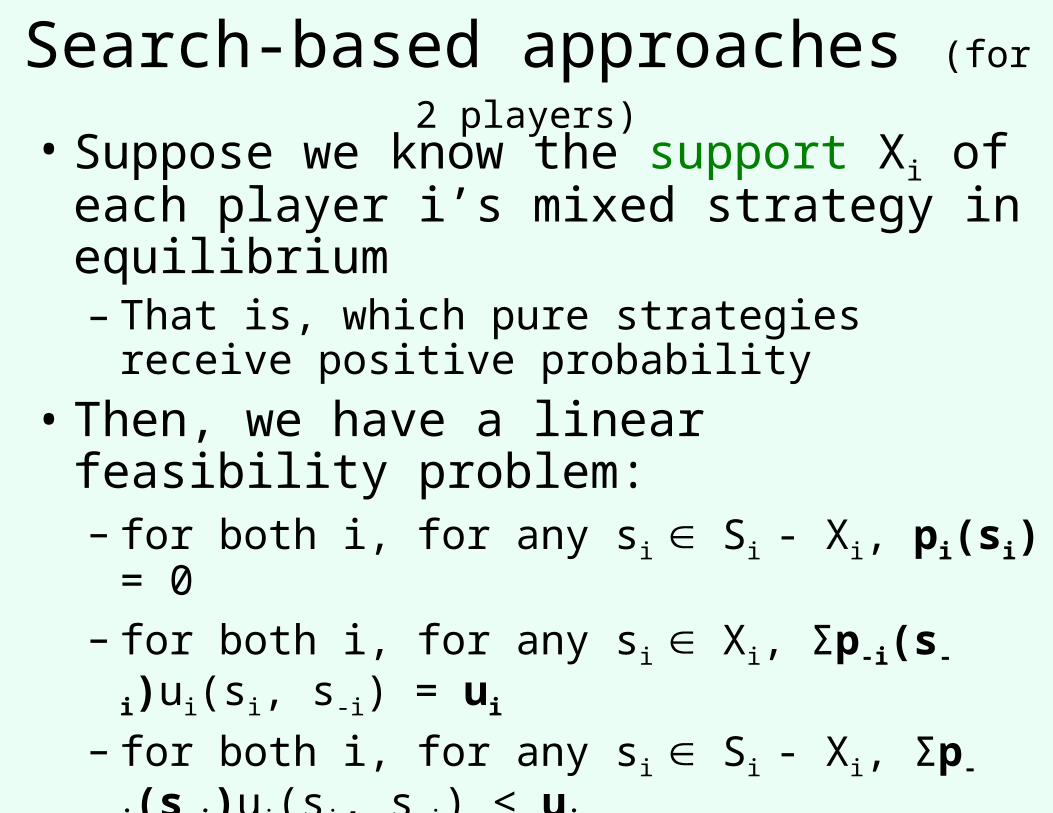
Search-based approaches (for 2 players)

• Suppose we know the support Xi of each player i’s mixed strategy in equilibrium– That is, which pure strategies receive positive

probability

• Then, we have a linear feasibility problem:– for both i, for any si Si - Xi, pi(si) = 0– for both i, for any si Xi, Σp-i(s-i)ui(si, s-i) = ui

– for both i, for any si Si - Xi, Σp-i(s-i)ui(si, s-i) ≤ ui

• Thus, we can search over possible supports– This is the basic idea underlying methods in

[Dickhaut & Kaplan 91; Porter, Nudelman, Shoham AAAI04/GEB08]

• Dominated strategies can be eliminated

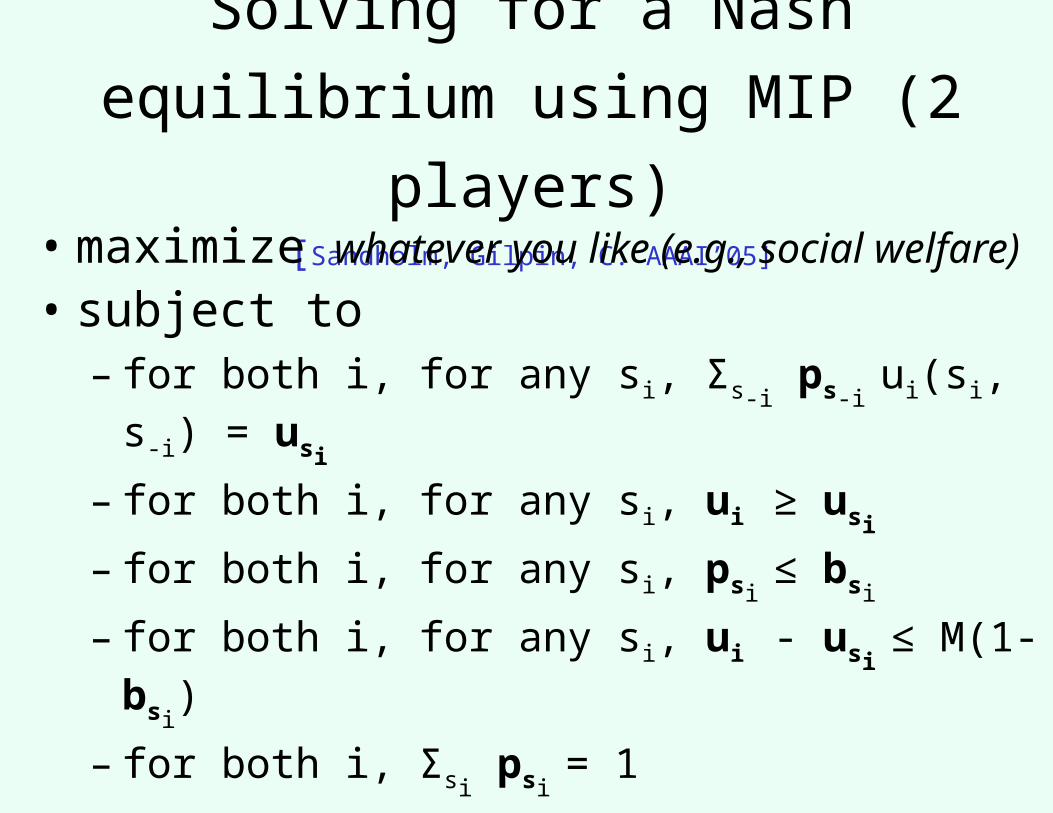
Solving for a Nash equilibrium

using MIP (2 players)[Sandholm, Gilpin, C. AAAI’05]

• maximize whatever you like (e.g., social welfare)

• subject to – for both i, for any si, Σs-i

ps-i ui(si, s-i) = usi

– for both i, for any si, ui ≥ usi

– for both i, for any si, psi ≤ bsi

– for both i, for any si, ui - usi

≤ M(1- bsi)

– for both i, Σsi psi

= 1

• bsi is a binary variable indicating whether si is

in the support, M is a large number

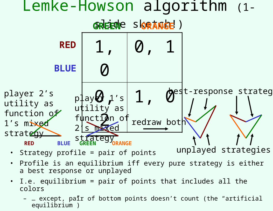
Lemke-Howson algorithm (1-slide sketch!)

• Strategy profile = pair of points

• Profile is an equilibrium iff every pure strategy is either a best response or unplayed

• I.e. equilibrium = pair of points that includes all the colors– … except, pair of bottom points doesn’t count (the “artificial equilibrium”)

• Walk in some direction from the artificial equilibrium; at each step, throw out the color used twice

1, 0 0, 10, 2 1, 0

RED

BLUE

GREEN ORANGE

player 2’s utility as function of 1’s mixed strategy

BLUERED GREEN ORANGE

player 1’s utility as function of 2’s mixed strategy redraw both

unplayed strategies

best-response strategies

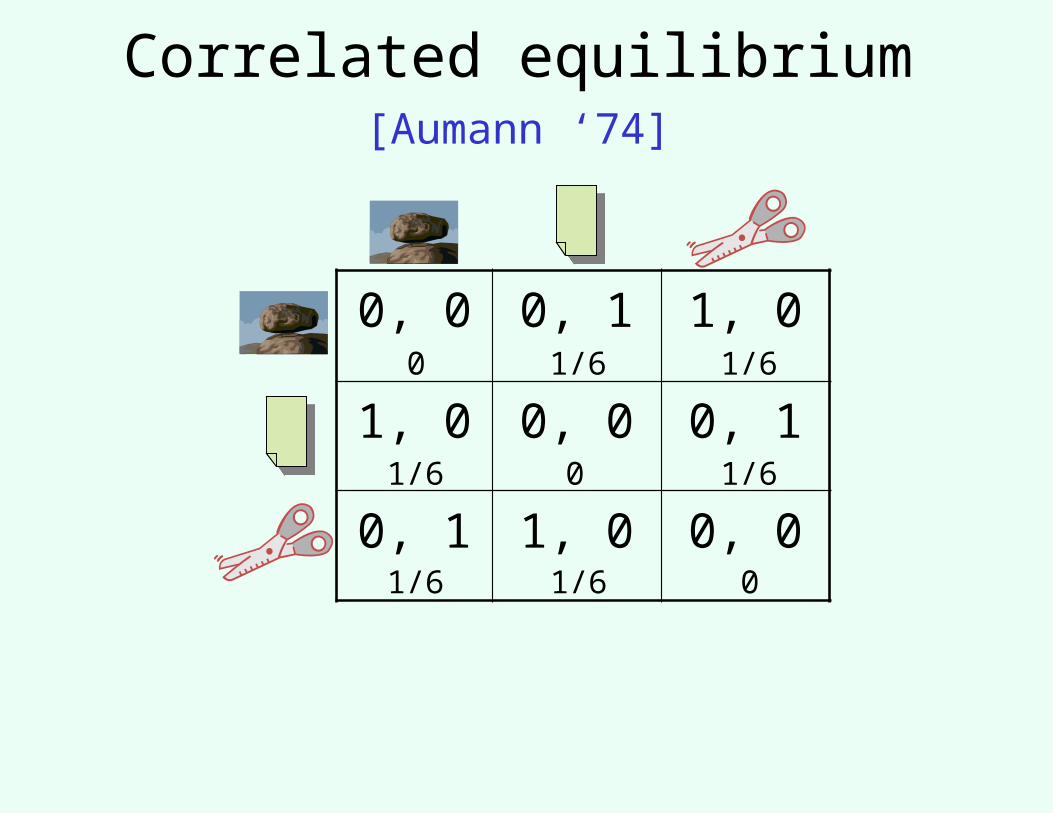
Correlated equilibrium [Aumann ‘74]

0, 0 0, 1 1, 0

1, 0 0, 0 0, 1

0, 1 1, 0 0, 0

1/6 1/6

1/6 1/6

1/61/6

0

0

0

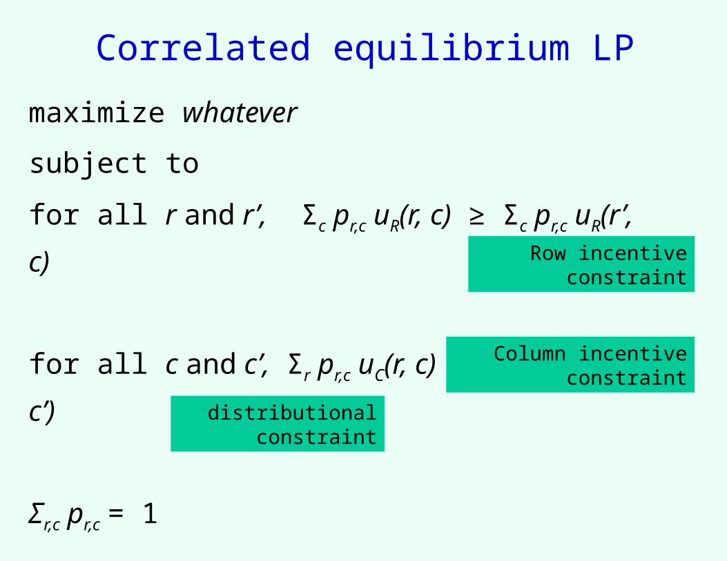
Correlated equilibrium LPmaximize whatever

subject to

for all r and r’, Σc pr,c uR(r, c) ≥ Σc pr,c uR(r’, c)

for all c and c’, Σr pr,c uC(r, c) ≥ Σr pr,c uC(r, c’)

Σr,c pr,c = 1distributional constraint

Row incentive constraint

Column incentive constraint

Recent developments

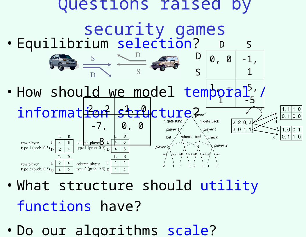
Questions raised by security games

• Equilibrium selection?

• How should we model temporal / information

structure?

• What structure should utility functions have?

• Do our algorithms scale?

0, 0 -1, 1

1, -1 -5, -5

D

S

D S

2, 2 -1, 0

-7, -8 0, 0

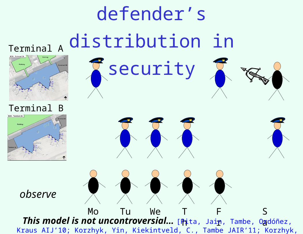
Observing the defender’s

distribution in securityTerminal A

Terminal B

Mo Tu We Th Fr Sa

observe

This model is not uncontroversial… [Pita, Jain, Tambe, Ordóñez, Kraus AIJ’10; Korzhyk, Yin, Kiekintveld, C., Tambe JAIR’11; Korzhyk, C., Parr AAMAS’11]

Commitment (Stackelberg strategies)

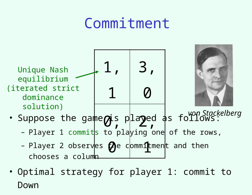
Commitment

1, 1 3, 0

0, 0 2, 1

• Suppose the game is played as follows:

– Player 1 commits to playing one of the rows,

– Player 2 observes the commitment and then chooses a column

• Optimal strategy for player 1: commit to Down

Unique Nash equilibrium (iterated

strict dominance solution)

von Stackelberg

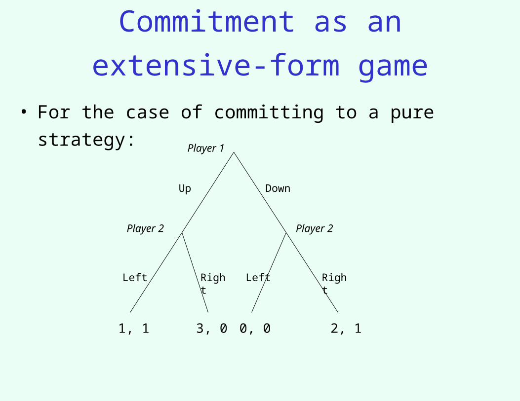
Commitment as an

extensive-form game

Player 1

Player 2 Player 2

1, 1 3, 0 0, 0 2, 1

• For the case of committing to a pure strategy:

Up Down

Left Left RightRight

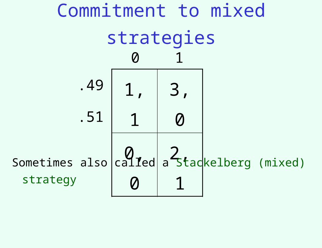
Commitment to mixed strategies

1, 1 3, 0

0, 0 2, 1

.49

.51

0 1

Sometimes also called a Stackelberg (mixed) strategy

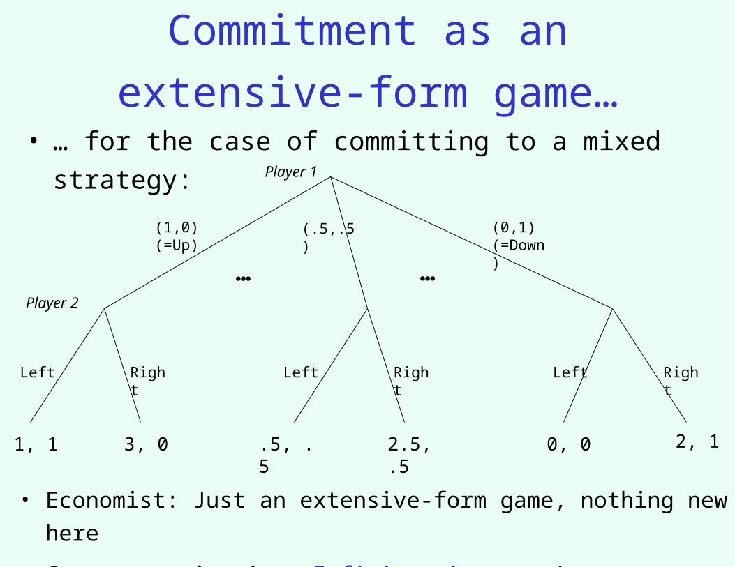
Commitment as an

extensive-form game…

Player 1

Player 2

1, 1 3, 0 0, 0 2, 1

• … for the case of committing to a mixed strategy:

(1,0) (=Up)

Left Left RightRight

.5, .5 2.5, .5

Left Right

(0,1) (=Down)

(.5,.5)

… …

• Economist: Just an extensive-form game, nothing new here

• Computer scientist: Infinite-size game! Representation matters

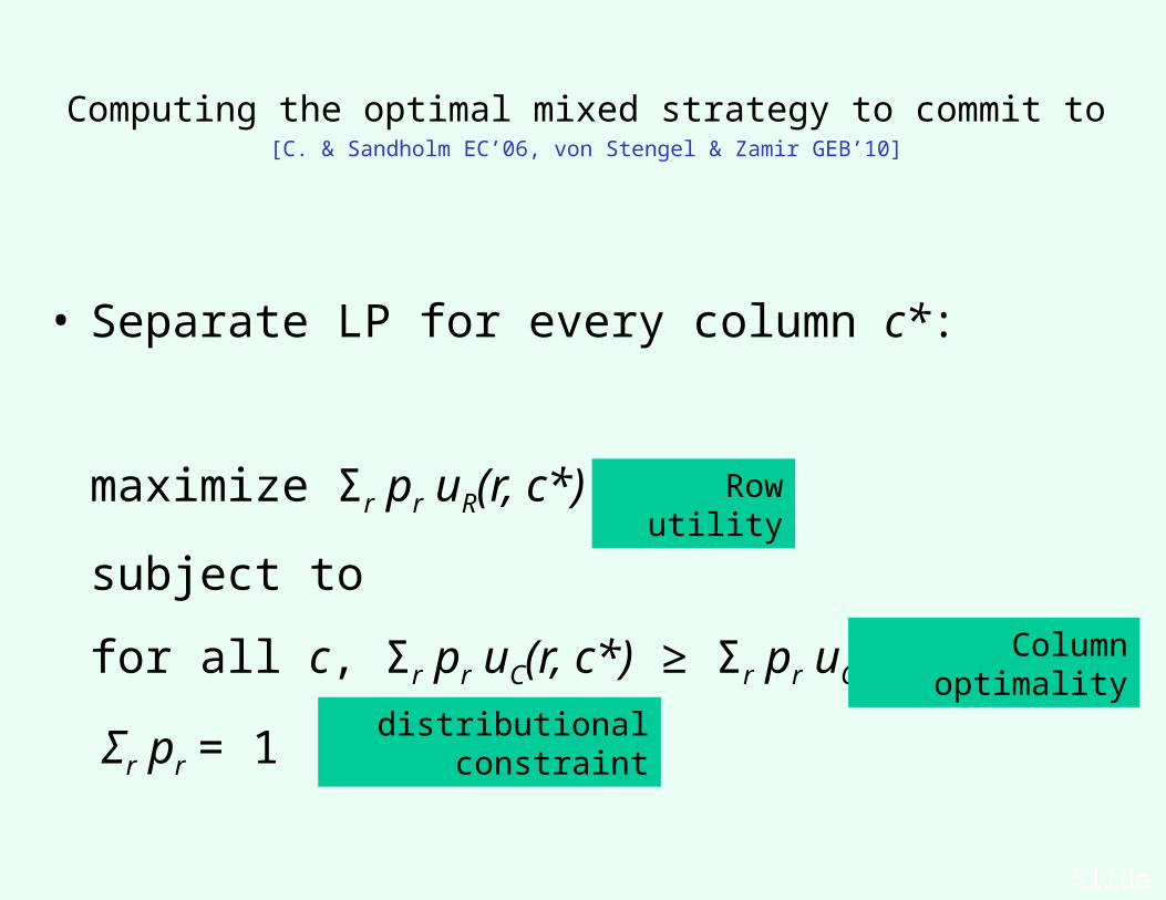
Computing the optimal mixed strategy to commit to[C. & Sandholm EC’06, von Stengel & Zamir GEB’10]

• Separate LP for every column c*:

maximize Σr pr uR(r, c*)

subject to

for all c, Σr pr uC(r, c*) ≥ Σr pr uC(r, c)

Σr pr = 1

Slide 7

Row utility

distributional constraint

Column optimality

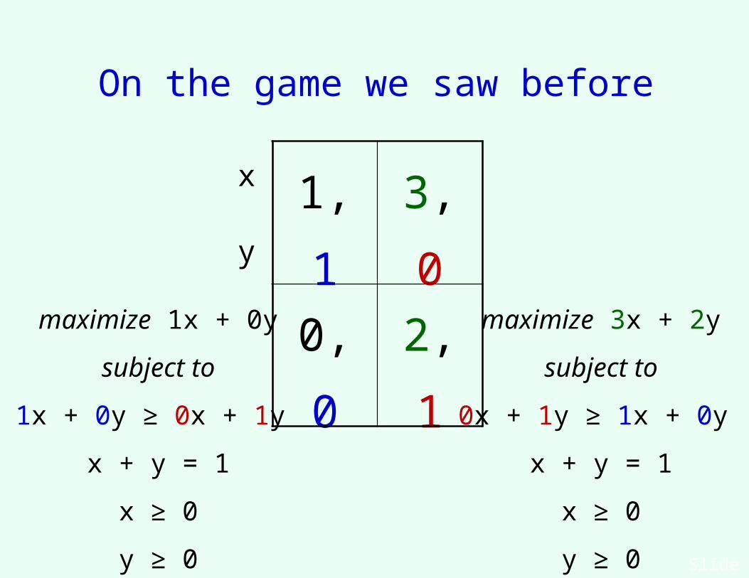
On the game we saw before

Slide 7

1, 1 3, 0

0, 0 2, 1maximize 1x + 0y

subject to

1x + 0y ≥ 0x + 1y

x + y = 1

x ≥ 0

y ≥ 0

maximize 3x + 2y

subject to

0x + 1y ≥ 1x + 0y

x + y = 1

x ≥ 0

y ≥ 0

x

y

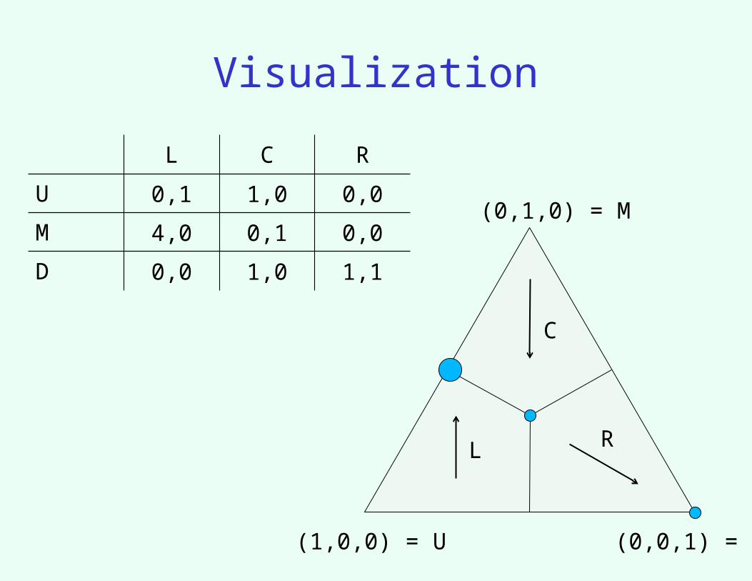
Visualization

L C R

U 0,1 1,0 0,0

M 4,0 0,1 0,0

D 0,0 1,0 1,1

(1,0,0) = U

(0,1,0) = M

(0,0,1) = D

L

C

R

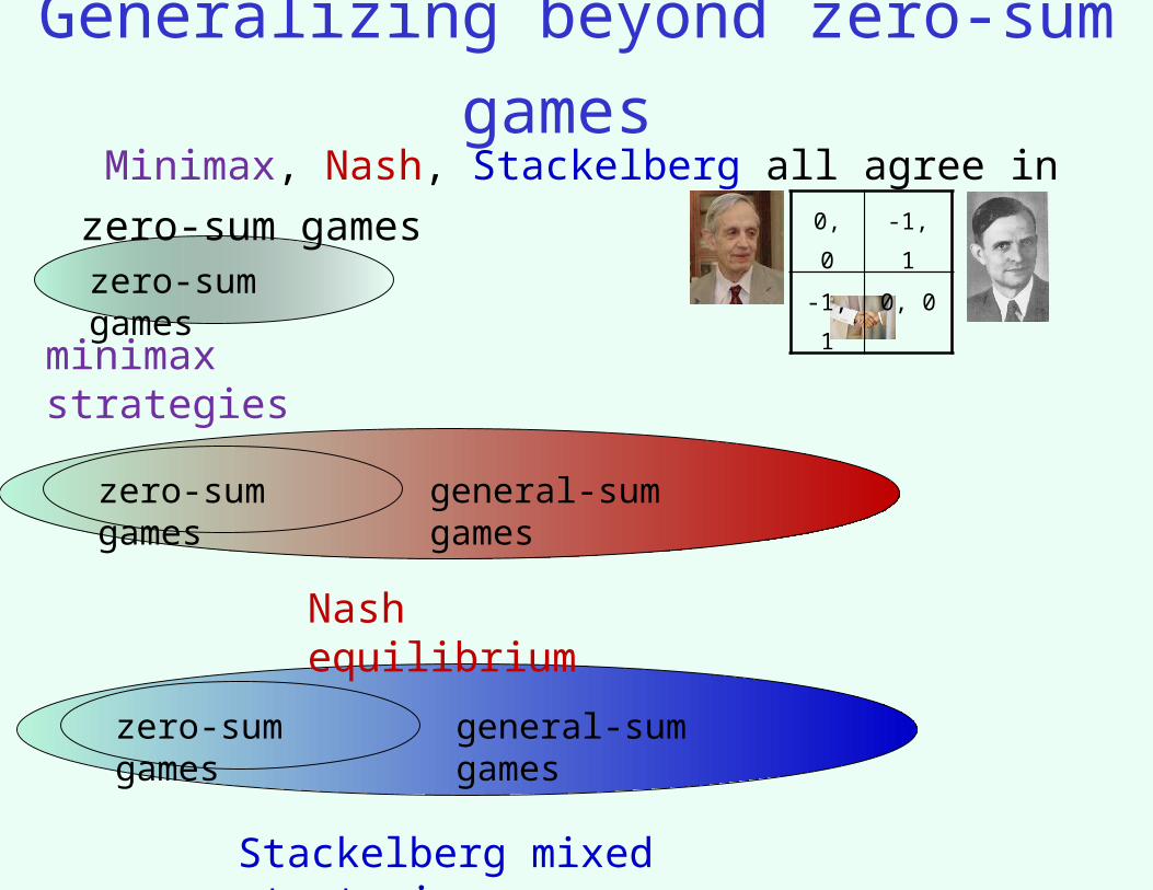
Generalizing beyond zero-sum games

general-sum games

zero-sum games

zero-sum games

general-sum games

Nash equilibrium

Stackelberg mixed strategies

zero-sum games

minimax strategies

Minimax, Nash, Stackelberg all agree in zero-sum games0, 0 -1, 1

-1, 1 0, 0

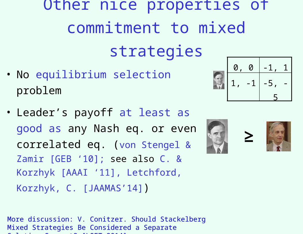
Other nice properties of

commitment to mixed strategies

• No equilibrium selection problem

• Leader’s payoff at least as good as

any Nash eq. or even correlated eq.

(von Stengel & Zamir [GEB ‘10]; see also C.

& Korzhyk [AAAI ‘11], Letchford, Korzhyk, C.

[JAAMAS’14])

≥

0, 0 -1, 1

1, -1 -5, -5

More discussion: V. Conitzer. Should Stackelberg Mixed Strategies Be Considered a Separate Solution Concept? [LOFT 2014]

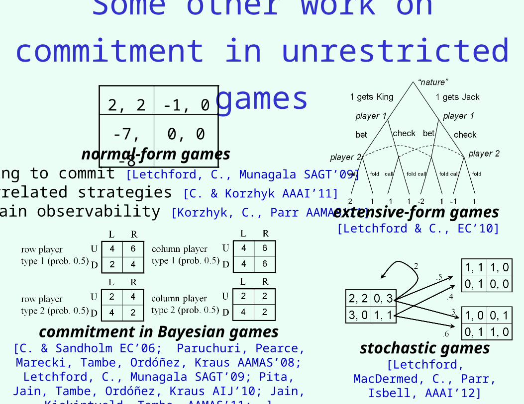
Some other work on commitment in

unrestricted games2, 2 -1, 0

-7, -8 0, 0

normal-form gameslearning to commit [Letchford, C., Munagala SAGT’09]

correlated strategies [C. & Korzhyk AAAI’11]

uncertain observability [Korzhyk, C., Parr AAMAS’11] extensive-form games [Letchford & C., EC’10]

commitment in Bayesian games[C. & Sandholm EC’06; Paruchuri, Pearce, Marecki, Tambe,

Ordóñez, Kraus AAMAS’08; Letchford, C., Munagala SAGT’09; Pita, Jain, Tambe, Ordóñez, Kraus AIJ’10; Jain,

Kiekintveld, Tambe AAMAS’11; …]

stochastic games[Letchford, MacDermed, C.,

Parr, Isbell, AAAI’12]

Security games

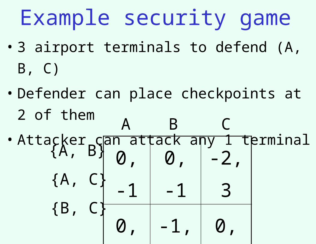
Example security game• 3 airport terminals to defend (A, B, C)

• Defender can place checkpoints at 2 of them

• Attacker can attack any 1 terminal

0, -1 0, -1 -2, 3

0, -1 -1, 1 0, 0

-1, 1 0, -1 0, 0

{A, B}

{A, C}

{B, C}

A B C

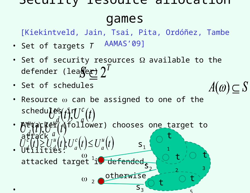
• Set of targets T

• Set of security resources W available to the defender (leader)

• Set of schedules

• Resource w can be assigned to one of the schedules in

• Attacker (follower) chooses one target to attack

• Utilities: if the attacked target is defended,

otherwise

•

Security resource allocation games[Kiekintveld, Jain, Tsai, Pita, Ordóñez, Tambe AAMAS’09]

w1

w2

s1

s2

s3

t5

t1

t2t3

t4

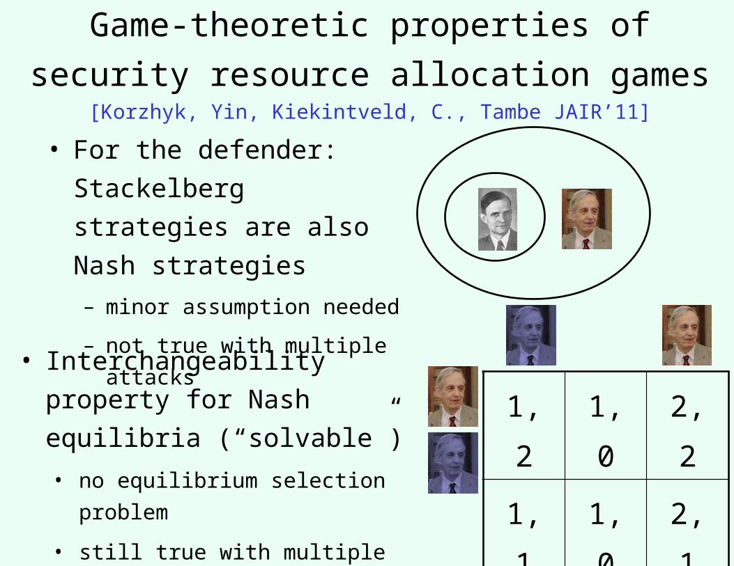
Game-theoretic properties of security resource

allocation games [Korzhyk, Yin, Kiekintveld, C., Tambe JAIR’11]

• For the defender:

Stackelberg strategies are

also Nash strategies

– minor assumption needed

– not true with multiple attacks

• Interchangeability property for

Nash equilibria (“solvable”)

• no equilibrium selection problem

• still true with multiple attacks [Korzhyk, C., Parr IJCAI’11]

1, 2 1, 0 2, 2

1, 1 1, 0 2, 1

0, 1 0, 0 0, 1

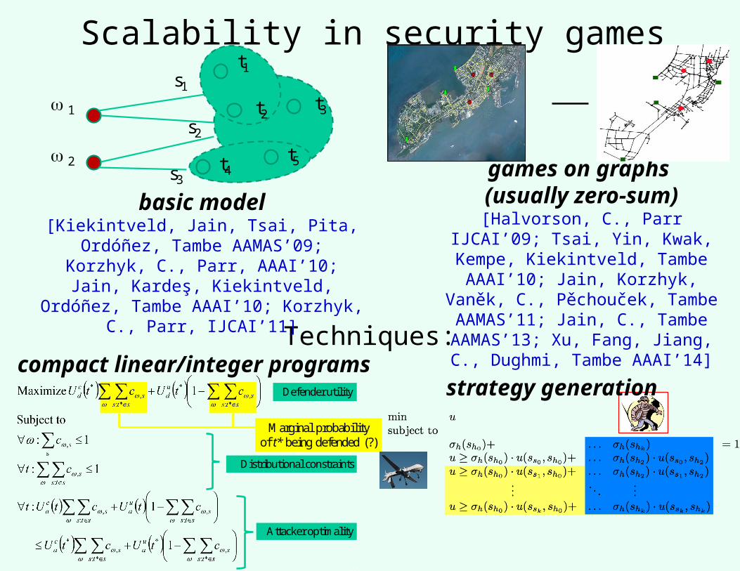
Scalability in security games

Techniques:

w 1

w 2

s1

s2

s3

t5

t1

t2t3

t4

basic model[Kiekintveld, Jain, Tsai, Pita, Ordóñez, Tambe

AAMAS’09; Korzhyk, C., Parr, AAAI’10; Jain, Kardeş, Kiekintveld, Ordóñez, Tambe

AAAI’10; Korzhyk, C., Parr, IJCAI’11]

games on graphs (usually zero-sum)

[Halvorson, C., Parr IJCAI’09; Tsai, Yin, Kwak, Kempe, Kiekintveld, Tambe AAAI’10; Jain, Korzhyk, Vaněk, C.,

Pěchouček, Tambe AAMAS’11; Jain, C., Tambe AAMAS’13; Xu, Fang, Jiang, C.,

Dughmi, Tambe AAAI’14]

Defender utility

Distributional constraints

Attacker optimality

Marginal probability of t* being defended (?)

Slide 11

compact linear/integer programsstrategy generation

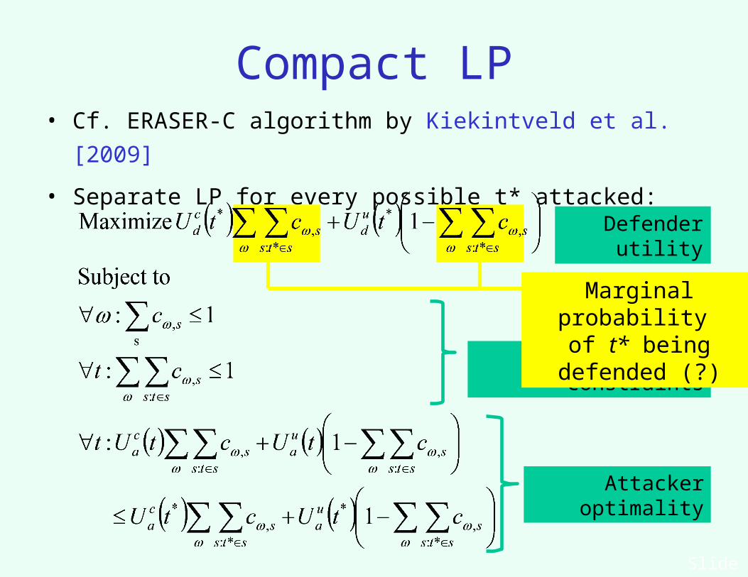
Compact LP• Cf. ERASER-C algorithm by Kiekintveld et al. [2009]

• Separate LP for every possible t* attacked:

Defender utility

Distributional constraints

Attacker optimality

Marginal probability of t* being defended (?)

Slide 11

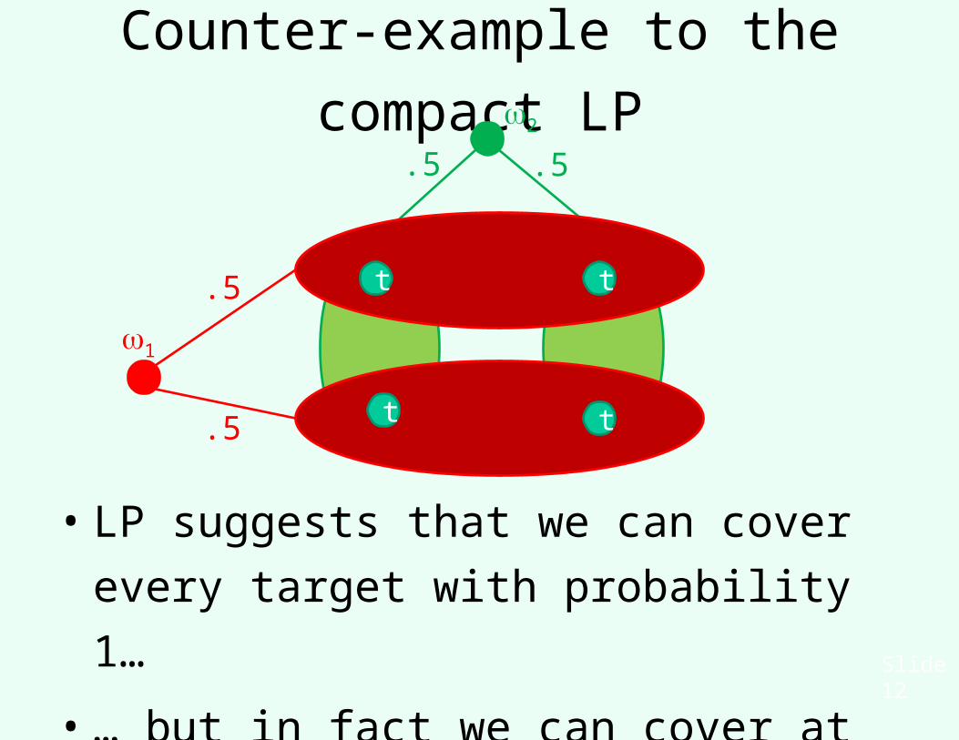
Counter-example to the compact LP

• LP suggests that we can cover every

target with probability 1…

• … but in fact we can cover at most 3

targets at a time

w1

w2

.5

.5

.5 .5

Slide 12

tt

t t

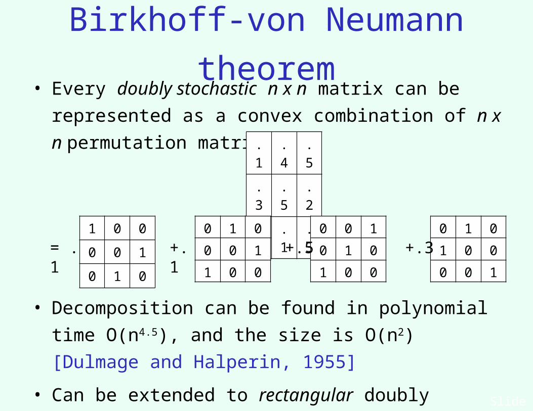
Birkhoff-von Neumann theorem• Every doubly stochastic n x n matrix can be

represented as a convex combination of n x n

permutation matrices

• Decomposition can be found in polynomial time O(n4.5),

and the size is O(n2) [Dulmage and Halperin, 1955]

• Can be extended to rectangular doubly substochastic

matrices

.1 .4 .5

.3 .5 .2

.6 .1 .3

1 0 0

0 0 1

0 1 0

= .10 1 0

0 0 1

1 0 0

+.10 0 1

0 1 0

1 0 0

+.50 1 0

1 0 0

0 0 1

+.3

Slide 14

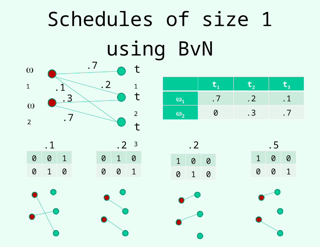
Schedules of size 1 using BvN

w1

w2

t1

t2

t3

.7

.1

.7

.3

.2 t1 t2 t3

w1 .7 .2 .1

w2 0 .3 .7

0 0 1

0 1 0

0 1 0

0 0 11 0 0

0 1 0

1 0 0

0 0 1

.1 .2.2 .5

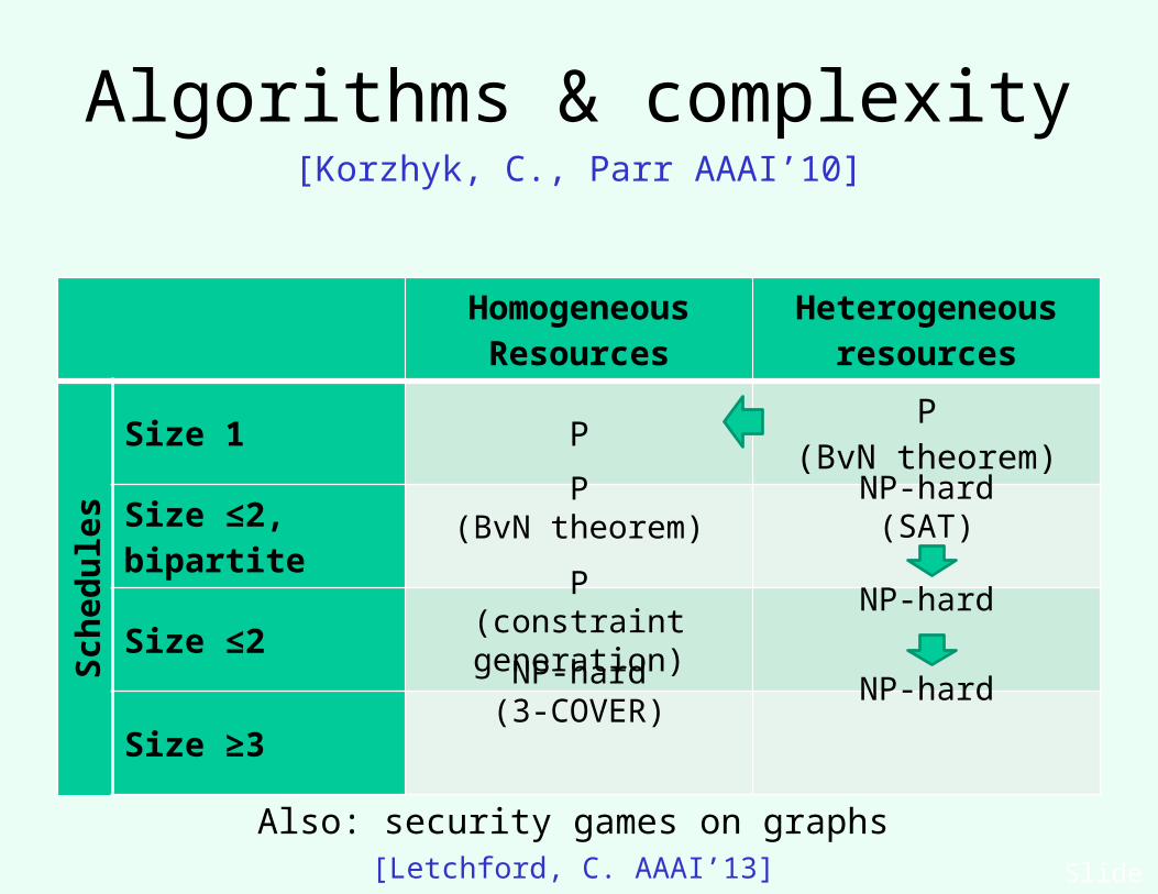
Algorithms & complexity[Korzhyk, C., Parr AAAI’10]

HomogeneousResources

Heterogeneousresources

Schedules

Size 1 PP

(BvN theorem)

Size ≤2, bipartite

Size ≤2

Size ≥3

P(BvN theorem)

P(constraint generation)

NP-hard(SAT)

NP-hard

NP-hardNP-hard(3-COVER)

Slide 16

Also: security games on graphs[Letchford, C. AAAI’13]

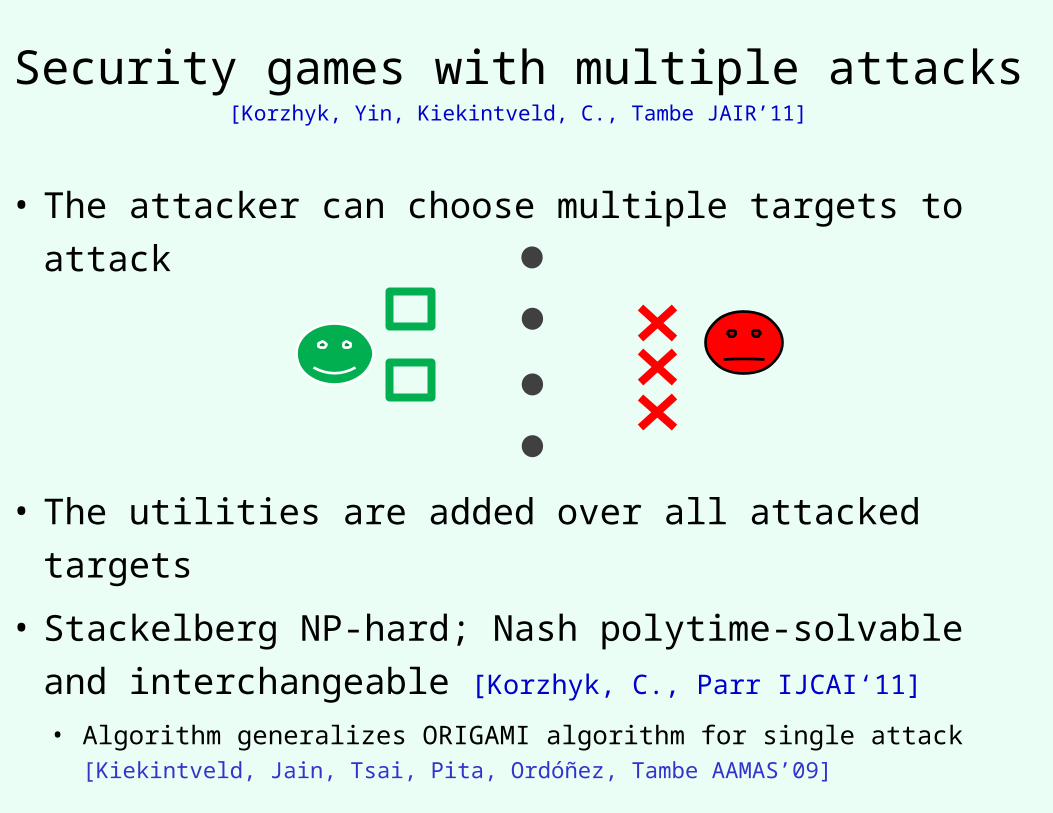
Security games with multiple attacks[Korzhyk, Yin, Kiekintveld, C., Tambe JAIR’11]

• The attacker can choose multiple targets to attack

• The utilities are added over all attacked targets

• Stackelberg NP-hard; Nash polytime-solvable and

interchangeable [Korzhyk, C., Parr IJCAI‘11]

• Algorithm generalizes ORIGAMI algorithm for single attack [Kiekintveld, Jain, Tsai, Pita, Ordóñez, Tambe AAMAS’09]

Day 1 Day 2 Day 3 Day 4 Day 5 Day 6 Day 7

Cou

nt

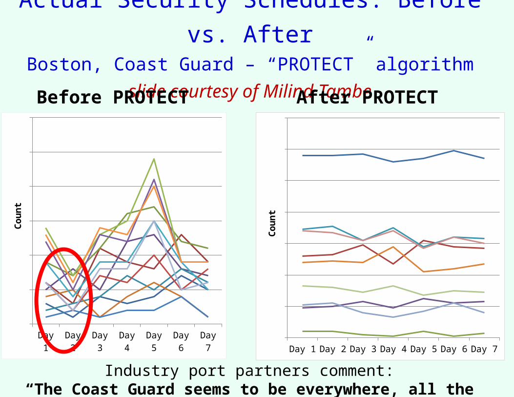
Actual Security Schedules: Before vs. AfterBoston, Coast Guard – “PROTECT” algorithm

slide courtesy of Milind TambeBefore PROTECT After PROTECT

Day 1 Day 2 Day 3 Day 4 Day 5 Day 6 Day 7

Cou

nt

Industry port partners comment:“The Coast Guard seems to be everywhere, all the time."

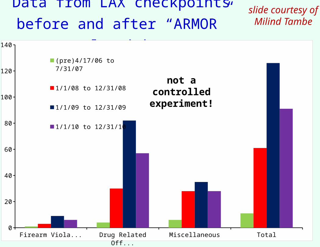
Data from LAX checkpoints

before and after “ARMOR” algorithm

slide

Firearm Violations Drug Related Offenses Miscellaneous Total0

20

40

60

80

100

120

140

(pre)4/17/06 to 7/31/07

1/1/08 to 12/31/08

1/1/09 to 12/31/09

1/1/10 to 12/31/10

slide courtesy of Milind Tambe

not a controlled experiment!

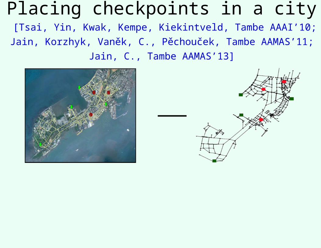
Placing checkpoints in a city [Tsai, Yin, Kwak, Kempe, Kiekintveld, Tambe AAAI’10; Jain, Korzhyk,

Vaněk, C., Pěchouček, Tambe AAMAS’11; Jain, C., Tambe AAMAS’13]

Learning in games

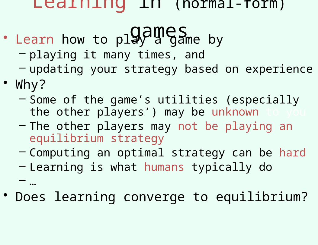
Learning in (normal-form) games• Learn how to play a game by

– playing it many times, and – updating your strategy based on experience

• Why?– Some of the game’s utilities (especially the other

players’) may be unknown to you– The other players may not be playing an equilibrium

strategy– Computing an optimal strategy can be hard– Learning is what humans typically do– …

• Does learning converge to equilibrium?

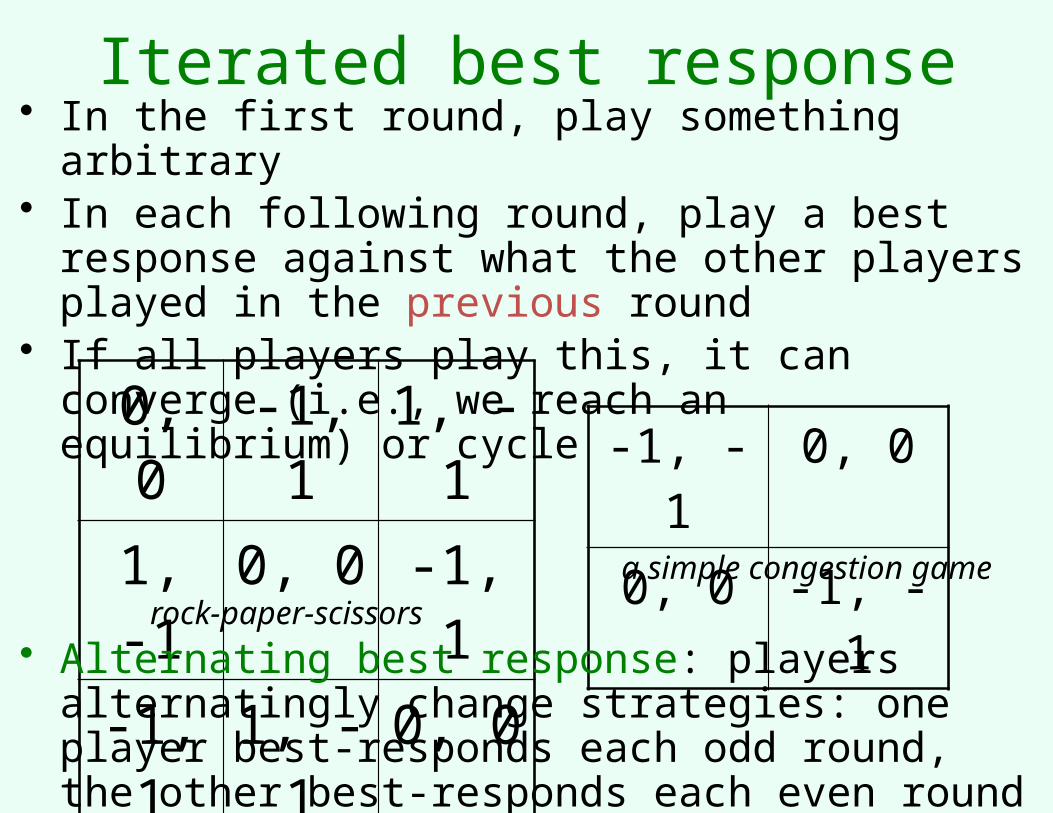
Iterated best response

0, 0 -1, 1 1, -11, -1 0, 0 -1, 1-1, 1 1, -1 0, 0

• In the first round, play something arbitrary• In each following round, play a best response against

what the other players played in the previous round• If all players play this, it can converge (i.e., we reach

an equilibrium) or cycle

-1, -1 0, 0

0, 0 -1, -1

• Alternating best response: players alternatingly change strategies: one player best-responds each odd round, the other best-responds each even round

rock-paper-scissors

a simple congestion game

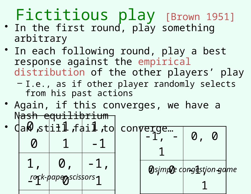
Fictitious play [Brown 1951]

0, 0 -1, 1 1, -1

1, -1 0, 0 -1, 1

-1, 1 1, -1 0, 0

• In the first round, play something arbitrary• In each following round, play a best response against

the empirical distribution of the other players’ play– I.e., as if other player randomly selects from his past

actions• Again, if this converges, we have a Nash equilibrium• Can still fail to converge…

-1, -1 0, 0

0, 0 -1, -1

rock-paper-scissorsa simple congestion game

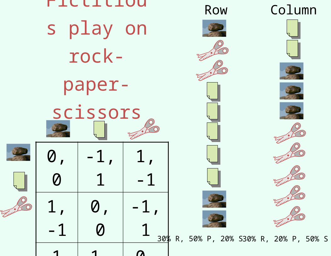
Fictitious

play on

rock-paper-

scissors

0, 0 -1, 1 1, -1

1, -1 0, 0 -1, 1

-1, 1 1, -1 0, 0

Row Column

30% R, 50% P, 20% S 30% R, 20% P, 50% S

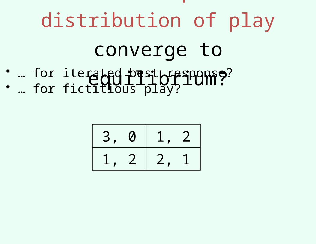
Does the empirical distribution

of play converge to equilibrium?• … for iterated best response?• … for fictitious play?

3, 0 1, 2

1, 2 2, 1

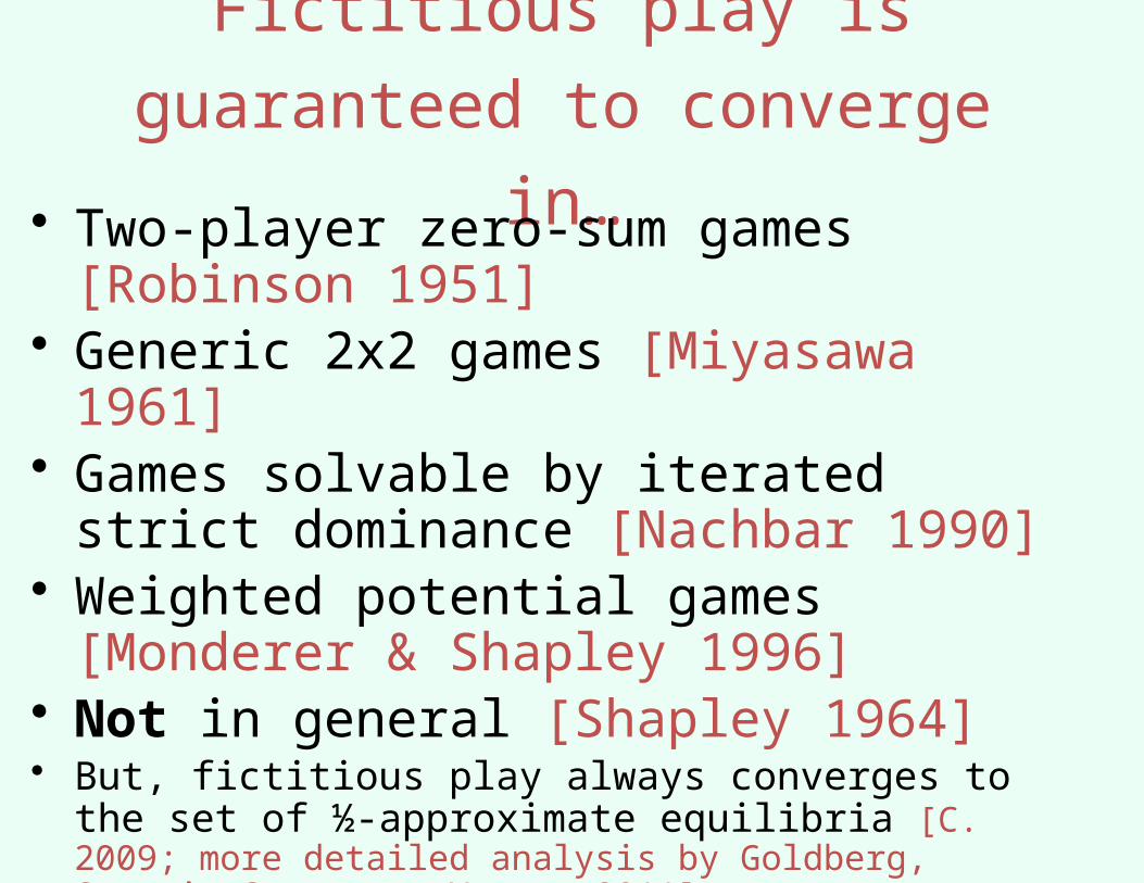
Fictitious play is guaranteed to

converge in…• Two-player zero-sum games [Robinson

1951]• Generic 2x2 games [Miyasawa 1961]• Games solvable by iterated strict

dominance [Nachbar 1990]• Weighted potential games [Monderer &

Shapley 1996]• Not in general [Shapley 1964]• But, fictitious play always converges to the set of ½-

approximate equilibria [C. 2009; more detailed analysis by Goldberg, Savani, Sørensen, Ventre 2011]

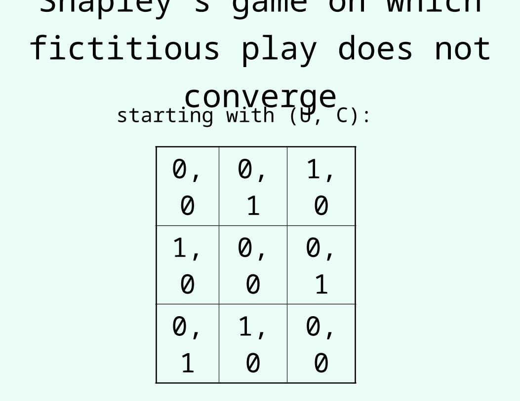
Shapley’s game on which fictitious

play does not convergestarting with (U, C):

0, 0 0, 1 1, 01, 0 0, 0 0, 10, 1 1, 0 0, 0

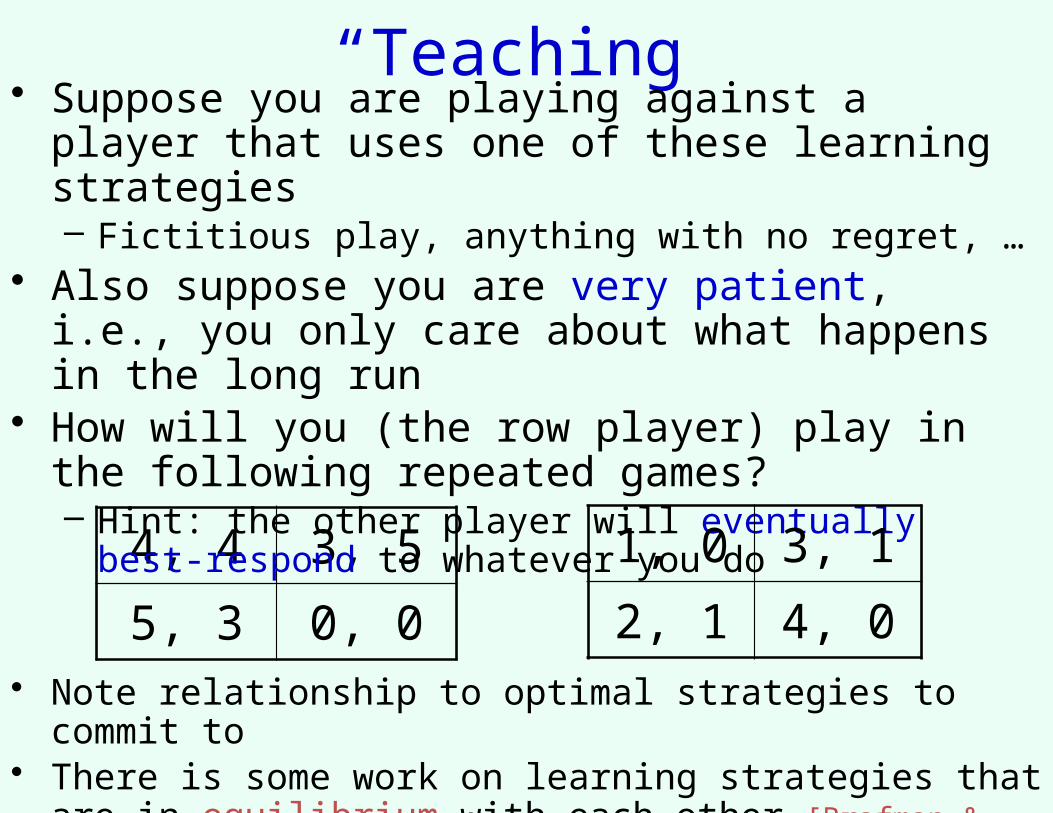
“Teaching”

4, 4 3, 5

5, 3 0, 0

• Suppose you are playing against a player that uses one of these learning strategies– Fictitious play, anything with no regret, …

• Also suppose you are very patient, i.e., you only care about what happens in the long run

• How will you (the row player) play in the following repeated games?– Hint: the other player will eventually best-respond to

whatever you do

1, 0 3, 1

2, 1 4, 0

• Note relationship to optimal strategies to commit to• There is some work on learning strategies that are in

equilibrium with each other [Brafman & Tennenholtz AIJ04]

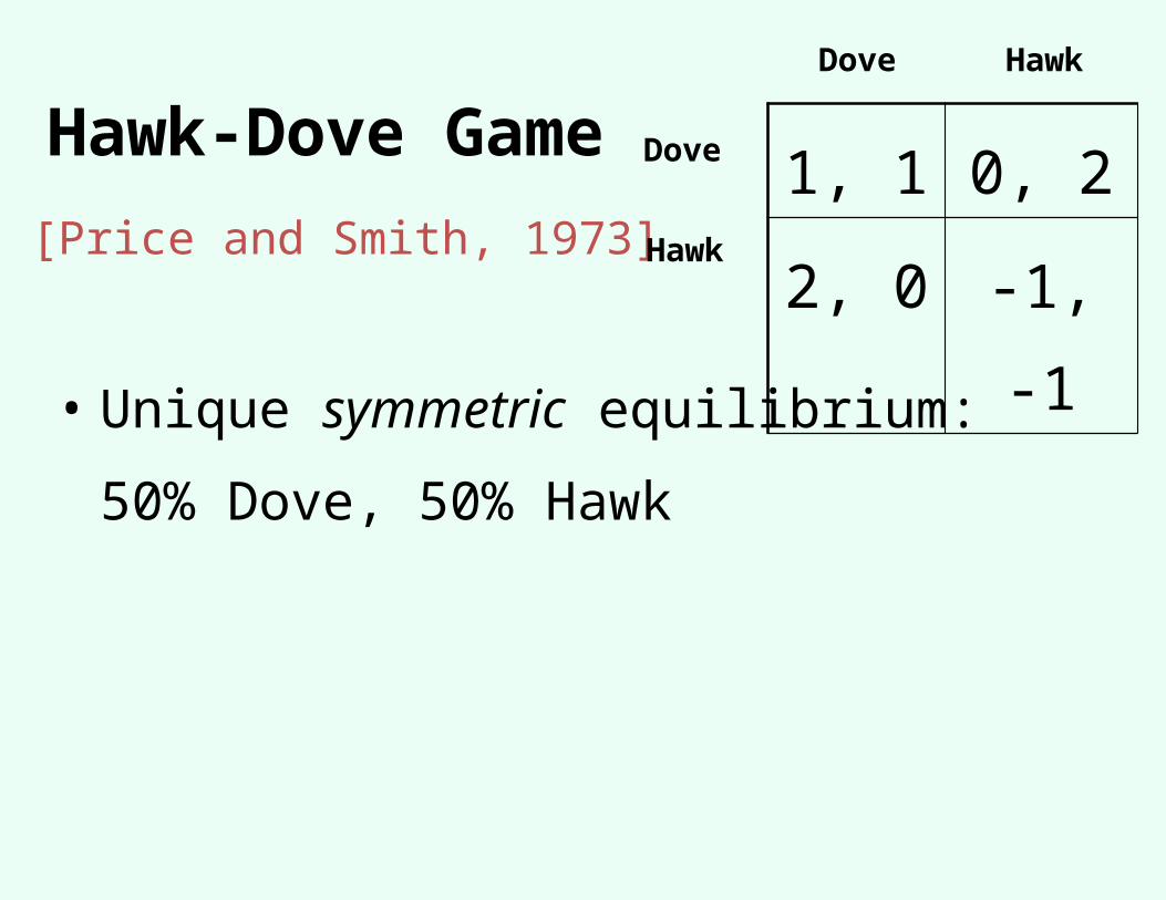
Hawk-Dove Game

[Price and Smith, 1973]

• Unique symmetric equilibrium:

50% Dove, 50% Hawk

1, 1 0, 2

2, 0 -1, -1

Dove

Dove

Hawk

Hawk

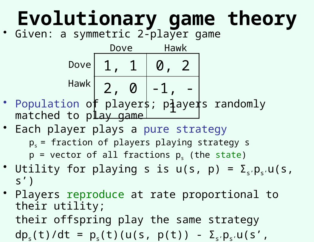
Evolutionary game theory• Given: a symmetric 2-player game

1, 1 0, 2

2, 0 -1, -1

Dove

Dove

Hawk

Hawk

• Population of players; players randomly matched to play game

• Each player plays a pure strategyps = fraction of players playing strategy s

p = vector of all fractions ps (the state)

• Utility for playing s is u(s, p) = Σs’ps’u(s, s’)• Players reproduce at rate proportional to their utility;

their offspring play the same strategy

dps(t)/dt = ps(t)(u(s, p(t)) - Σs’ps’u(s’, p(t)))– Replicator dynamic

• What are the steady states?

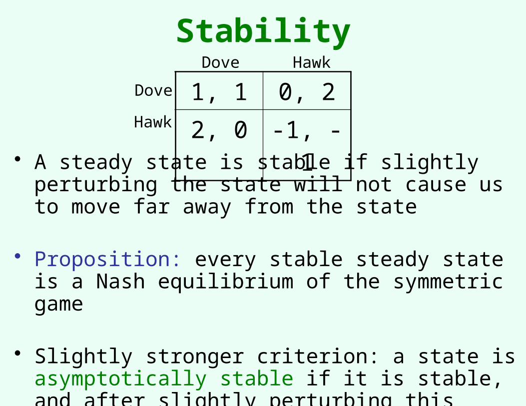
Stability

• A steady state is stable if slightly perturbing the state will not cause us to move far away from the state

• Proposition: every stable steady state is a Nash equilibrium of the symmetric game

• Slightly stronger criterion: a state is asymptotically stable if it is stable, and after slightly perturbing this state, we will (in the limit) return to this state

1, 1 0, 2

2, 0 -1, -1

Dove

Dove

Hawk

Hawk

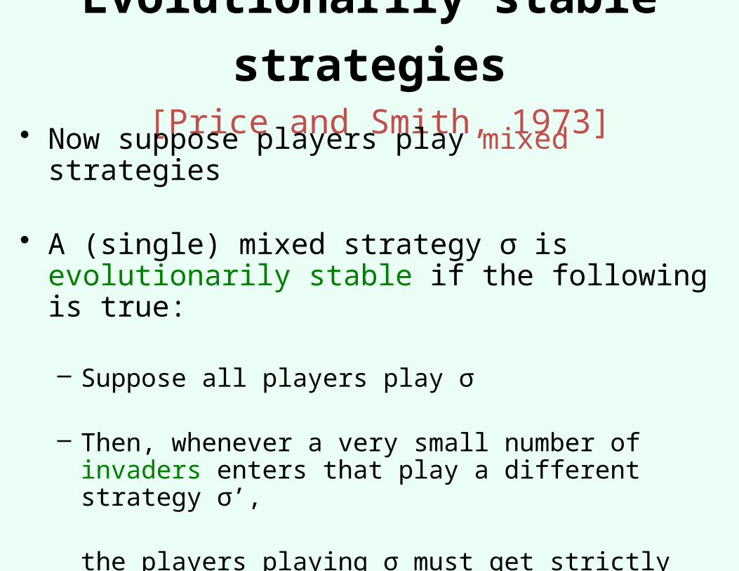
Evolutionarily stable strategies [Price and Smith, 1973]

• Now suppose players play mixed strategies

• A (single) mixed strategy σ is evolutionarily stable if the following is true:

– Suppose all players play σ

– Then, whenever a very small number of invaders enters that play a different strategy σ’,

the players playing σ must get strictly higher utility than those playing σ’ (i.e., σ must be able to repel invaders)

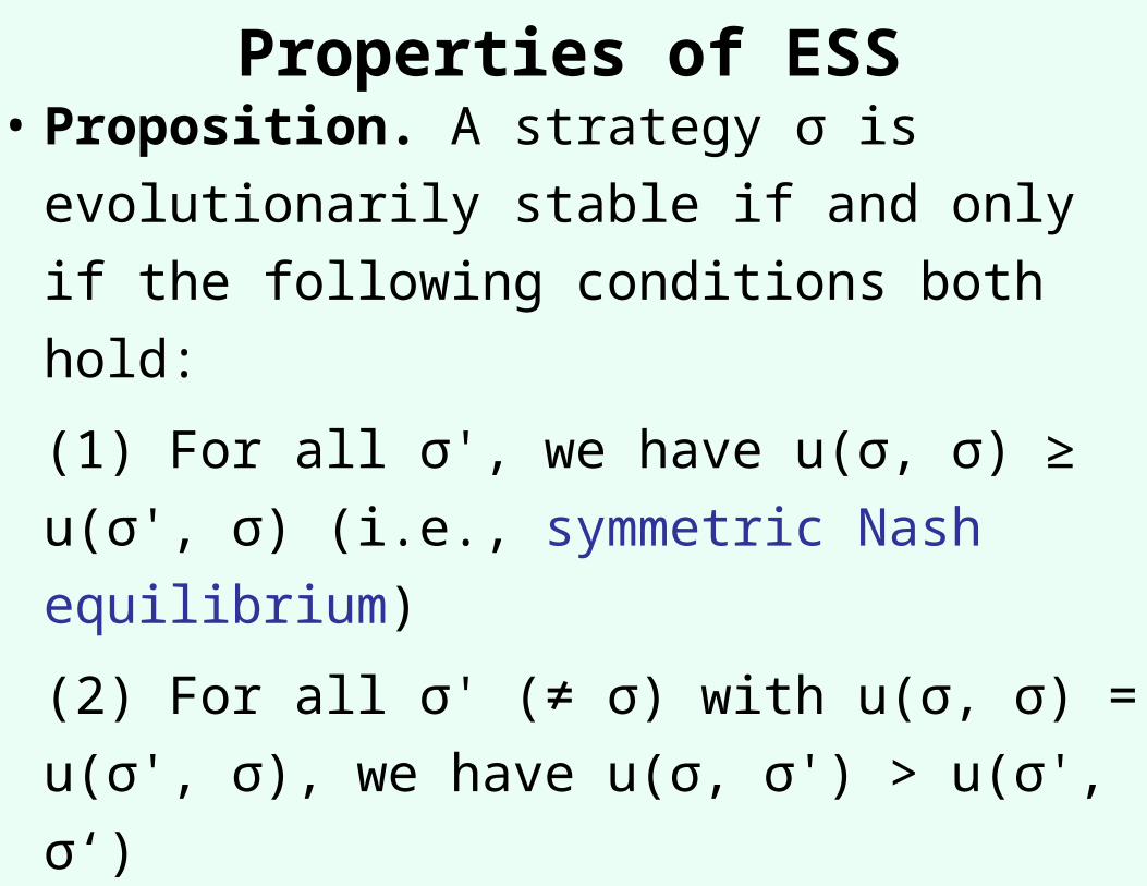
Properties of ESS• Proposition. A strategy σ is evolutionarily

stable if and only if the following conditions both

hold:

(1) For all σ', we have u(σ, σ) ≥ u(σ', σ) (i.e.,

symmetric Nash equilibrium)

(2) For all σ' (≠ σ) with u(σ, σ) = u(σ', σ), we

have u(σ, σ') > u(σ', σ‘)

• Theorem [Taylor and Jonker 1978, Hofbauer et al. 1979, Zeeman 1980].

Every ESS is asymptotically stable under the

replicator dynamic. (Converse does not hold [van Damme 1987].)

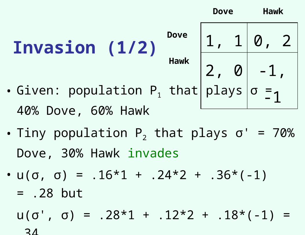
Invasion (1/2)

• Given: population P1 that plays σ = 40% Dove,

60% Hawk

• Tiny population P2 that plays σ' = 70% Dove, 30%

Hawk invades

• u(σ, σ) = .16*1 + .24*2 + .36*(-1) = .28 but

u(σ', σ) = .28*1 + .12*2 + .18*(-1) = .34

• σ‘ (initially) grows in the population; invasion is

successful

1, 1 0, 2

2, 0 -1, -1

Dove

Dove

Hawk

Hawk

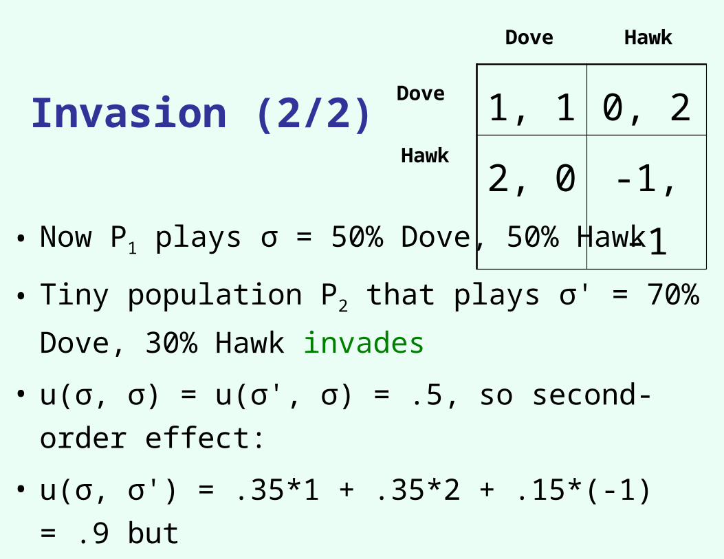
Invasion (2/2)

• Now P1 plays σ = 50% Dove, 50% Hawk

• Tiny population P2 that plays σ' = 70% Dove, 30%

Hawk invades

• u(σ, σ) = u(σ', σ) = .5, so second-order effect:

• u(σ, σ') = .35*1 + .35*2 + .15*(-1) = .9 but

u(σ', σ') = .49*1 + .21*2 + .09*(-1) = .82

• σ' shrinks in the population; invasion is repelled

1, 1 0, 2

2, 0 -1, -1

Dove

Dove

Hawk

Hawk

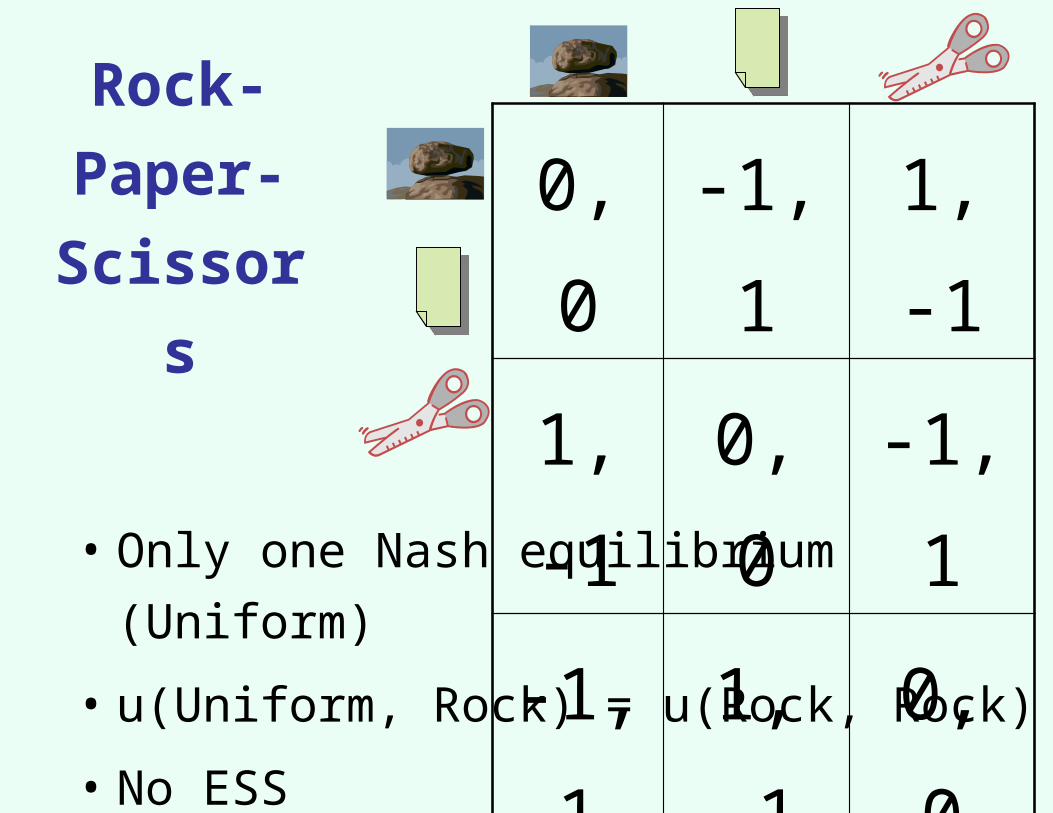
Rock-

Paper-

Scissors

• Only one Nash equilibrium (Uniform)

• u(Uniform, Rock) = u(Rock, Rock)

• No ESS

0, 0 -1, 1 1, -1

1, -1 0, 0 -1, 1

-1, 1 1, -1 0, 0

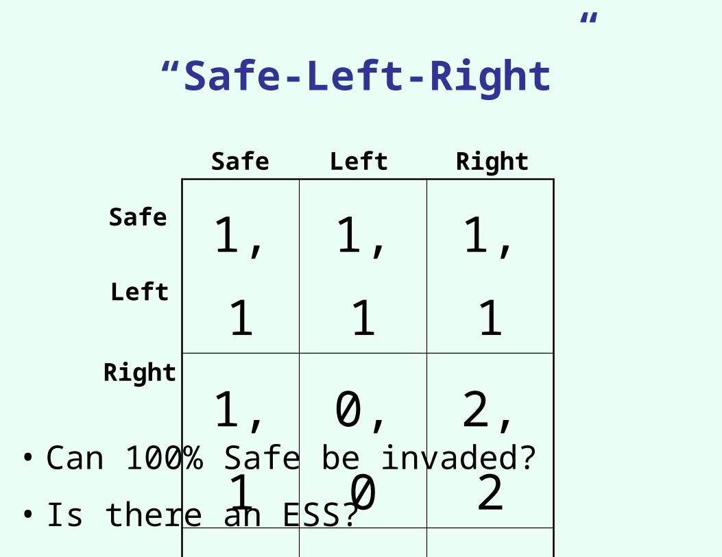
“Safe-Left-Right”

• Can 100% Safe be invaded?

• Is there an ESS?

1, 1 1, 1 1, 1

1, 1 0, 0 2, 2

1, 1 2, 2 0, 0

Safe

Safe Left Right

Right

Left

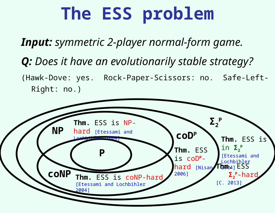
Input: symmetric 2-player normal-form game.

Q: Does it have an evolutionarily stable strategy?

(Hawk-Dove: yes. Rock-Paper-Scissors: no. Safe-Left-Right: no.)

P

NP

coNP

coDP

Σ2PThm. ESS is NP-hard

[Etessami and Lochbihler 2004].

Thm. ESS is coNP-hard [Etessami and Lochbihler 2004].

Thm. ESS is in Σ2

P [Etessami and

Lochbihler 2004].Thm. ESS is coDP-hard [Nisan 2006]. Thm. ESS is

Σ2P-hard [C.

2013].

The ESS problem

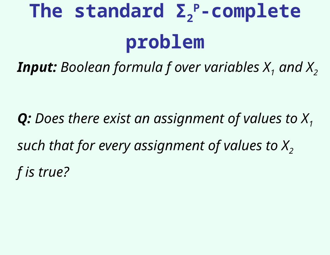
The standard Σ2P-complete problem

Input: Boolean formula f over variables X1 and X2

Q: Does there exist an assignment of values to X1

such that for every assignment of values to X2

f is true?

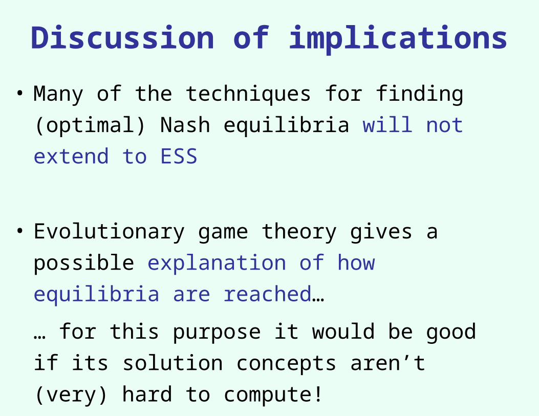
Discussion of implications

• Many of the techniques for finding (optimal) Nash

equilibria will not extend to ESS

• Evolutionary game theory gives a possible

explanation of how equilibria are reached…

… for this purpose it would be good if its solution

concepts aren’t (very) hard to compute!

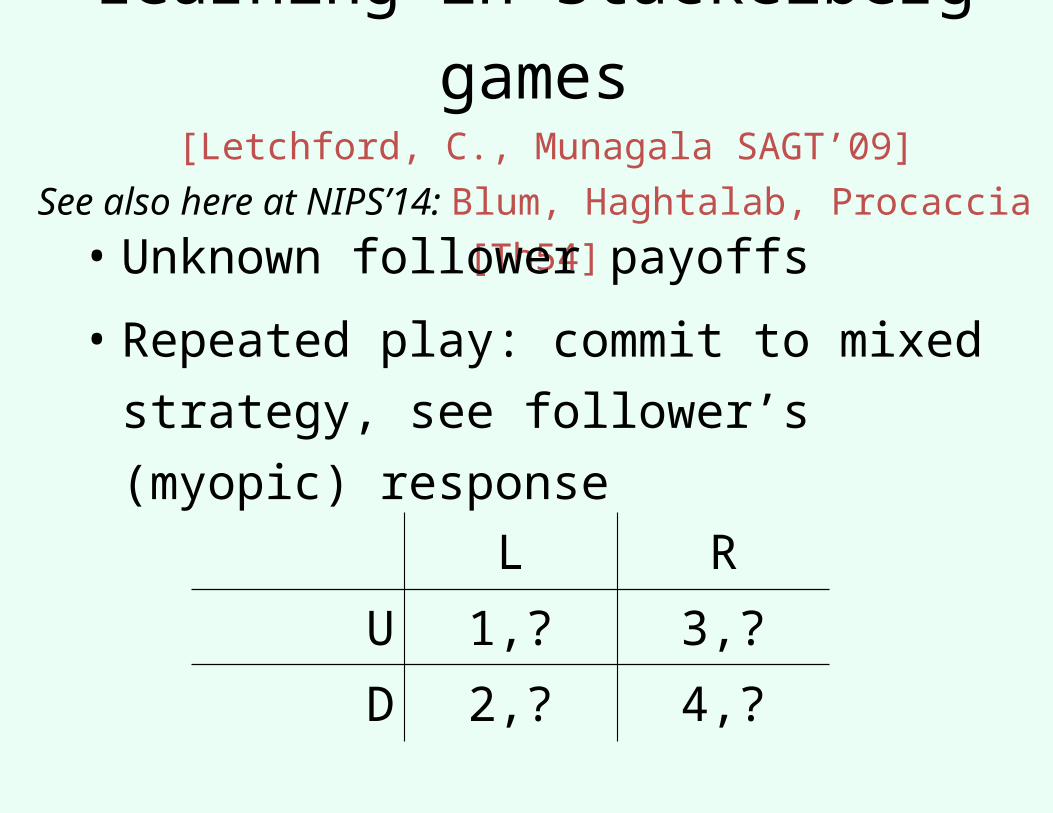
Learning in Stackelberg games [Letchford, C., Munagala SAGT’09]

See also here at NIPS’14: Blum, Haghtalab, Procaccia [Th54]

• Unknown follower payoffs

• Repeated play: commit to mixed strategy,

see follower’s (myopic) response

L R

U 1,? 3,?

D 2,? 4,?

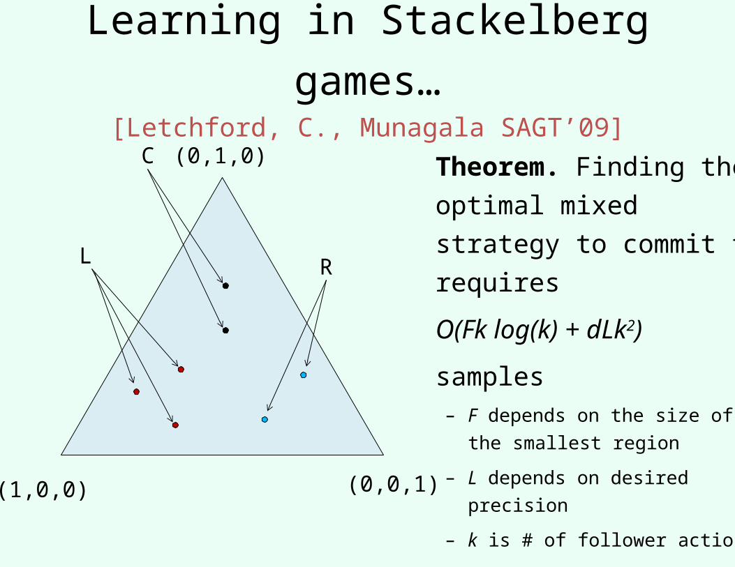
Learning in Stackelberg games…[Letchford, C., Munagala SAGT’09]

L R

C

(1,0,0) (0,0,1)

(0,1,0) Theorem. Finding the

optimal mixed strategy to

commit to requires

O(Fk log(k) + dLk2)

samples– F depends on the size of the

smallest region

– L depends on desired precision

– k is # of follower actions

– d is # of leader actions

Three main techniques in

the learning algorithm

• Find one point in each region (using

random sampling)

• Find a point on an unknown hyperplane

• Starting from a point on an unknown

hyperplane, determine the hyperplane

completely

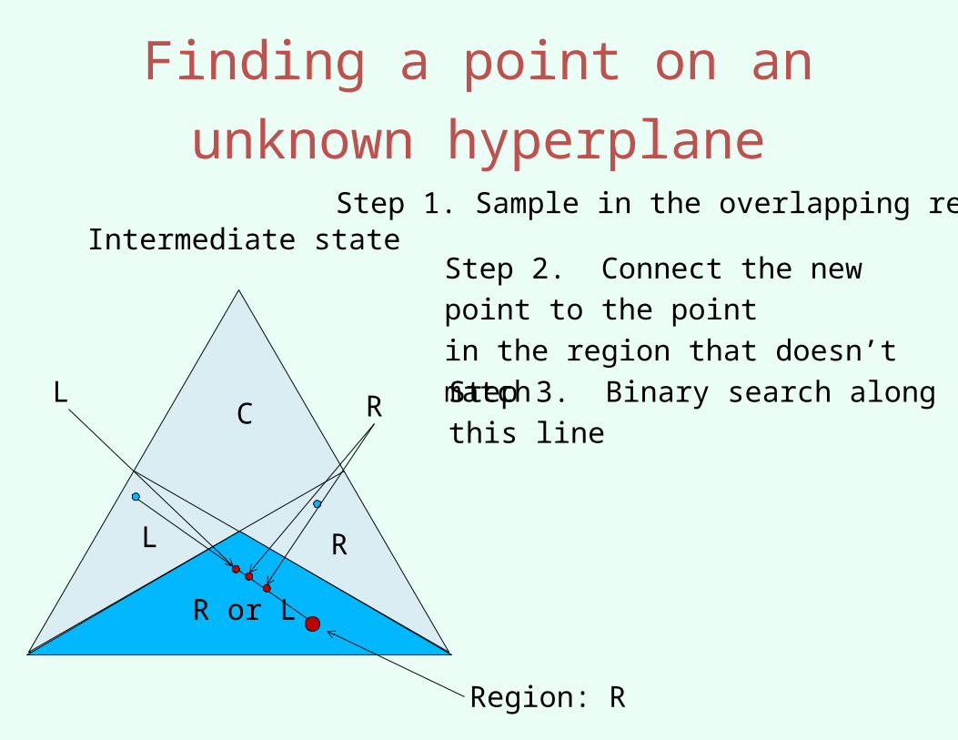
Finding a point on an unknown

hyperplane

L

C

R

R or L

Intermediate stateStep 1. Sample in the overlapping region

Region: R

Step 2. Connect the new point to the point

in the region that doesn’t match

Step 3. Binary search along this lineL R

Determining the hyperplane

L

C

R

R or L

Intermediate stateStep 1. Sample a regular d-simplex

centered at the point

Step 2. Connect d lines between points on

opposing sides

Step 3. Binary search along these lines

Step 4. Determine hyperplane (and update

the region estimates with this information)

L R

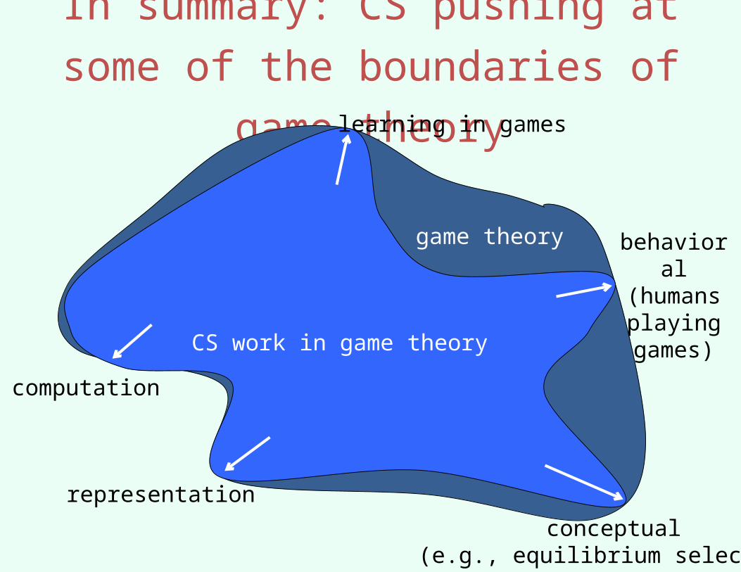
In summary: CS pushing at some of the

boundaries of game theory

conceptual(e.g., equilibrium selection)

computation

behavioral (humans playing games)

representation

learning in games

CS work in game theory

game theory