Digital Object Identifier (DOI) 10.1007/s00138-004-0160-7Machine Vision and Applications (2005) Machine Vision and

Applications

Computing depth maps from descent images

Yalin Xiong1, Clark F. Olson2, Larry H. Matthies3

1 KLA-Tencor, 160 Rio Robles St., San Jose, CA 95134, USA2 University of Washington, Computing and Software Systems, 18115 Campus Way NE, Box 358534, Bothell, WA 98011, USA3 Jet Propulsion Laboratory, California Institute of Technology, 4800 Oak Grove Drive, M/S 125-209, Pasadena, CA 91109, USA

Received: 7 November 2002 / Accepted: 13 September 2004Published online: 25 February 2005 – c© Springer-Verlag 2005

Abstract. In the exploration of the planets of our solar sys-tem, images taken during a lander’s descent to the surface ofa planet provide a critical link between orbital images andsurface images. The descent images not only allow us to lo-cate the landing site in a global coordinate frame, but theyalso provide progressively higher-resolution maps for missionplanning. This paper addresses the generation of depth mapsfrom the descent images. Our approach has two steps, motionrefinement and depth recovery. During motion refinement, weuse an initial motion estimate in order to avoid the intrinsic mo-tion ambiguity. The objective of the motion-refinement step isto adjust the motion parameters such that the reprojection er-ror is minimized. The depth-recovery step correlates adjacentframes to match pixels for triangulation. Due to the descend-ing motion, the conventional rectification process is replacedby a set of anti-aliasing image warpings corresponding to a setof virtual parallel planes. We demonstrate experimental resultson synthetic and real descent images.

Keywords: Planetary exploration – Structure from motion –Descent images – Motion estimation – Terrain mapping

1 Introduction

Future space missions that land on Mars (and other planetarybodies) may include a downward-looking camera mountedon the vehicle as it descends to the surface. Images taken bysuch a camera during the descent provide a critical link be-tween orbital images and lander/rover images on the surfaceof the planet. By matching the descent images against orbitalimages, the descent vehicle can localize itself in global co-ordinates and, therefore, achieve precision landing. Throughanalysis of the descent images, we can build a multiresolu-tion terrain map for safe landing, rover planning, navigation,and localization. This paper addresses the issue of generating

Correspondence to: Clark F. Olson(e-mail: cfolson@u.washington.edu,Tel.: +1-425-3525288, Fax: +1-425-3525216)

multiresolution terrain maps from a sequence of descent im-ages. We use motion-estimation and structure-from-motiontechniques to recover depth maps from the images. A newtechnique for computing depths is described that is based oncorrelating the images after performing anti-aliasing imagewarpings that correspond to a set of virtual planar surfaces.

It is well known that, when the viewed terrain is a planarsurface, the motion-recovery problem is ill-posed, since trans-lations parallel to the surface appear similar to rotations aboutaxes parallel to the surface. Motion recovery is, therefore, notgenerally reliable for this scenario. However, if we have an in-dependent means to measure the orientation of the camera, wecan obtain stable motion recovery. For planetary explorationmissions, such measurements can be provided by the inertialnavigation sensors on the landing spacecraft.

For space missions, it is likely that the motion will benearly perpendicular to the planetary surface. For the MarsPolar Lander mission, which was unable to return data dueto loss of the lander, it was planned that the camera wouldtake an image every time the distance to the ground halved.In other words, there would be roughly a scale factor of twobetween adjacent frames in the sequence. A similar scenario islikely in future missions. The large change of scale prohibitsus from tracking many features across several frames. Formost features, we limit our correlation and depth recovery toadjacent frames for this reason.

The descending motion also causes problems in correlat-ing the images. Since the epipoles are located near the centerof the images, it is not practical to rectify adjacent frames inthe same manner that traditional stereo techniques do. Instead,we perform a virtual rectification, resampling the images byconsidering a set of parallel planar surfaces through the terrain.Each surface corresponds to a projective warping between theadjacent images. The surface that yields the best correlation ateach pixel determines the depth estimate for that location. Thismethodology not only aligns images according to the epipo-lar lines but also equalizes the image scales using anti-aliasedwarpings.

Of course, many other approaches have been proposedfor recovering motion and depth from image sequences[2,4,6,8,11,14]. This work differs from most previous workin two ways. First, almost all of the motion is forward along

Yalin Xiong et al.: Computing depth maps from descent images

Terrain

I

I2

1

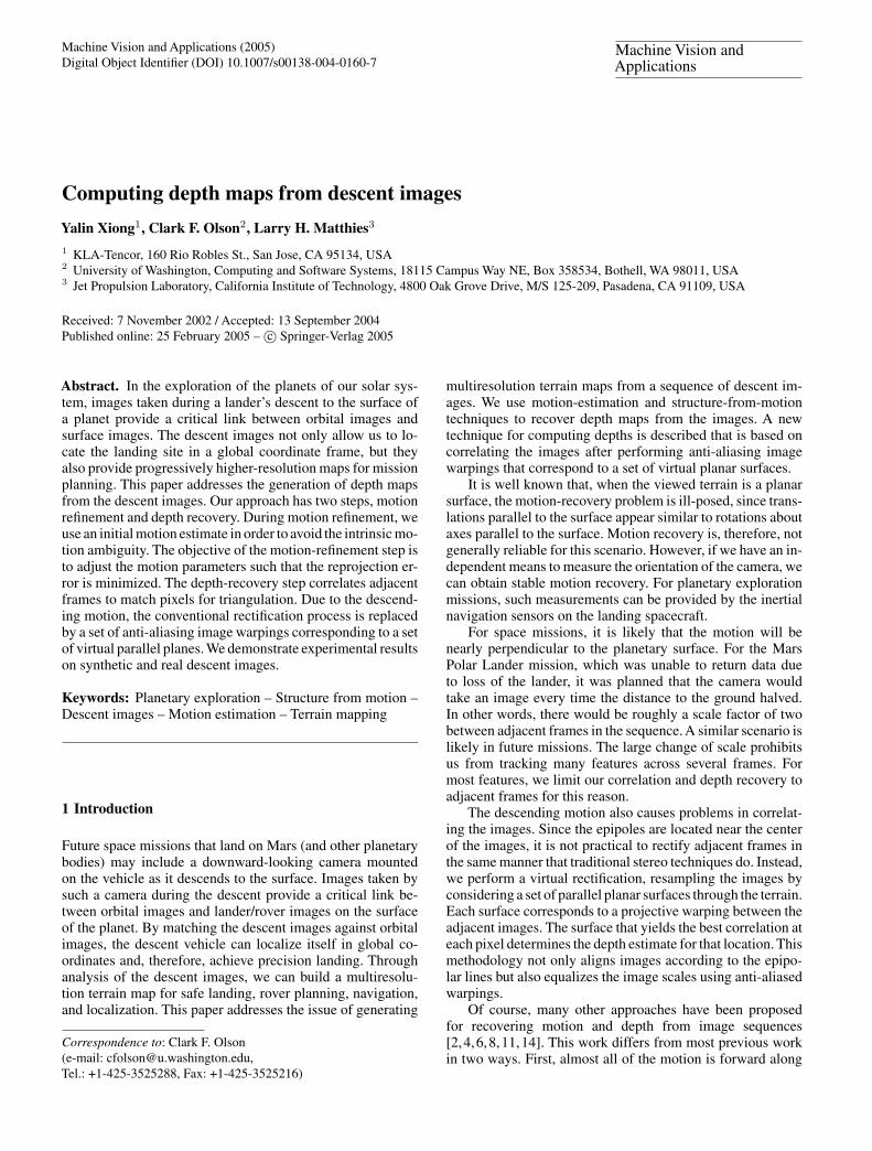
Fig. 1. Descent motion

the camera pointing direction. Second, large movements in thecamera position occur between frames, usually doubling theresolution of the images at each frame. This work is thus inpart, an application of previous work to the problem of map-ping spacecraft descent imagery and, in part, new techniquesfor dealing with the above problems. The technique producesdense maps of the terrain and operates under the full perspec-tive projection.

In the next two sections, we describe the motion-refinement and depth-recovery steps in detail. We then dis-cuss our experiments on synthetic and real descent images.The results demonstrate the various terrain features that canbe recovered. Near the landing site, small obstacles such asrocks and gullies can be identified for planning local rovernavigation. Further from the landing site, larger features suchas mountain slopes and cliffs are visible for use in long-rangeplanning.

2 Motion refinement

Recovering camera motion from two or more frames is oneof the classical problems in computer vision. Linear [7] andnonlinear [13] solutions have been proposed. Our scenario in-volves a downward motion towards a roughly planar surface(as in Fig. 1). Generic motion recovery from matched featuresis ill-posed owing to a numerical singularity (rotations andtranslations are difficult to distinguish.) Since the camera canbe rigidly attached to the lander, and the change in the landerorientation can be measured accurately by an inertial naviga-tion system onboard, we can eliminate the singularity prob-lem by adding a penalty term for deviating from the measuredorientation. The following two subsections briefly explain ourfeature correspondence and nonlinear optimization for motionrefinement.

2.1 Feature correspondence

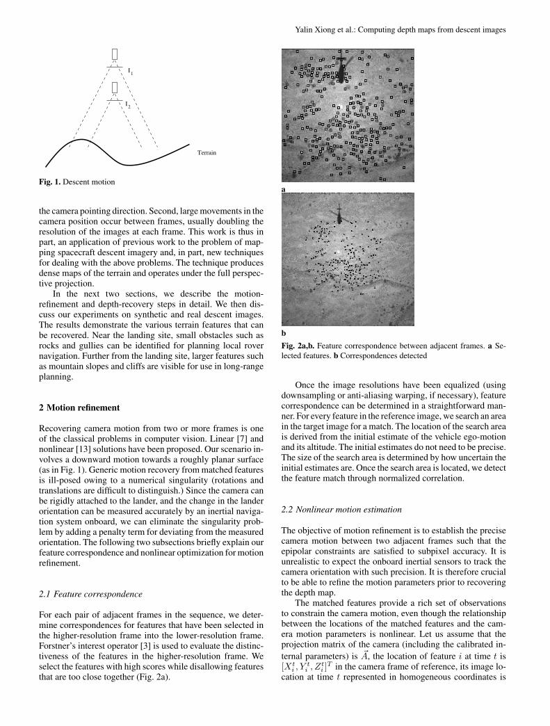
For each pair of adjacent frames in the sequence, we deter-mine correspondences for features that have been selected inthe higher-resolution frame into the lower-resolution frame.Forstner’s interest operator [3] is used to evaluate the distinc-tiveness of the features in the higher-resolution frame. Weselect the features with high scores while disallowing featuresthat are too close together (Fig. 2a).

a

b

Fig. 2a,b. Feature correspondence between adjacent frames. a Se-lected features. b Correspondences detected

Once the image resolutions have been equalized (usingdownsampling or anti-aliasing warping, if necessary), featurecorrespondence can be determined in a straightforward man-ner. For every feature in the reference image, we search an areain the target image for a match. The location of the search areais derived from the initial estimate of the vehicle ego-motionand its altitude. The initial estimates do not need to be precise.The size of the search area is determined by how uncertain theinitial estimates are. Once the search area is located, we detectthe feature match through normalized correlation.

2.2 Nonlinear motion estimation

The objective of motion refinement is to establish the precisecamera motion between two adjacent frames such that theepipolar constraints are satisfied to subpixel accuracy. It isunrealistic to expect the onboard inertial sensors to track thecamera orientation with such precision. It is therefore crucialto be able to refine the motion parameters prior to recoveringthe depth map.

The matched features provide a rich set of observationsto constrain the camera motion, even though the relationshipbetween the locations of the matched features and the cam-era motion parameters is nonlinear. Let us assume that theprojection matrix of the camera (including the calibrated in-ternal parameters) is �A, the location of feature i at time t is[Xt

i , Yti , Zt

i ]T in the camera frame of reference, its image lo-

cation at time t represented in homogeneous coordinates is

Yalin Xiong et al.: Computing depth maps from descent images

[xti, y

ti , z

ti ]

T , and the camera motion between time t and timet + 1 is composed of a translation �T and rotation �R (3×3matrix). The projection of the feature at time t is:

xt

iyt

izti

= �A

Xt

iY t

iZt

i

, (1)

and the projection at time (t + 1) is:xt+1

i

yt+1i

zt+1i

= �A

Xt+1

i

Y t+1i

Zt+1i

= �A

�R

Xt

iY t

iZt

i

+ �T

. (2)

Therefore, the feature motion in the image is:xt+1

i

yt+1i

zt+1i

= �A

�R �A−1

xt

iyt

izti

+ �T

= �U

xt

iyt

izti

+ �V , (3)

where �U = �A�R �A−1 is a 3×3 matrix and �V = �A�T is a 3-vector. Let [ct

i, rti ] = [xt

i/zti , y

ti/zt

i ] denote the actual columnand row location of feature i in image coordinates at time t.We then have the predicted feature locations at time t + 1 as:

ct+1i =

u00xti + u01y

ti + u02z

ti + v0

u20xti + u21yt

i + u22zti + v2

, (4)

rt+1i =

u10xti + u11y

ti + u12z

ti + v1

u20xti + u21yt

i + u22zti + v2

, (5)

where uij and vi are elements of �U and �V , respectively.There are two ways to optimize the camera motions in

the above equations. One is to reduce the two equations intoone by eliminating zt

i . We would then minimize the summeddeviation from the equation specifying a nonlinear relation be-tween [ct

i, rti ] and [ct+1

i , rt+1i ]. Though this method is concise

and simple, it poses a problem in the context of least-squaresminimization in that the objective function does not have aphysical meaning.

The other approach to refine the motion estimate is to aug-ment the parameters with depth estimates for each of the fea-tures. There are two advantages to this approach. First, the ob-jective function becomes the distance between the predictedand observed feature locations, which is a meaningful mea-sure for optimization. In addition, in the context of mappingdescent images, we have a good initial estimate of the depthvalue from the spacecraft altimeter. Incorporating this infor-mation will thus improve the optimization in general.

Let us say that the depth value of feature i at time t is dti and

the camera is pointing along the z-axis; the homogeneous co-ordinates of the feature are [xt

i, yti , z

ti ]

T = dti[c

ti, r

ti , 1]t. There-

fore, the overall objective function we are minimizing is:

N∑i=1

((ct+1i − ct+1

i

)2+

(rt+1i − rt+1

i

)2)

, (6)

where N is the number of features and ct+1i and rt+1

i arenonlinear functions of the camera motion and depth value dt

i

given by Eqs. 4 and 5. We perform nonlinear minimizationusing the Levenberg–Marquardt algorithm with the estimatedposition as the starting point. Robustness is improved throughthe use of robust statistics in the optimization.

The result of the optimization is a refined estimate of therotation R and translation T between the camera positions.In the optimization, we represent the rotation using a quater-nion. In order to resolve between translations and rotations,which appear similar, a penalty term is added to the objectivefunction Eq. 6 that prefers motions close to the initial motionestimate. This constrains the motion not to deviate far from theorientation estimated by navigation sensors while allowing forsome deviation in order to fit the observed data. An additionalpenalty term is added that forces the quaternion to have unitlength and, thus, correspond to a valid rotation matrix.

Equation 6 specifies the objective function for two adja-cent images. A long sequence of descending images requiresa common scale reference in order to build consistent mul-tiresolution depth maps. The key to achieving this is to trackfeatures over more than two images. From Eq. 3 the depthvalue of feature i at time t + 1 can be represented as

dt+1i

ct+1

i

rt+1i1

= �Udt

i

ct

irti1

+ �V . (7)

Thus, the overall objective is to minimize the sum of Eq. 6for all adjacent pairs while maintaining the consistent scalereference by imposing the constraint in Eq. 7 for all featurestracked over more than two frames.

3 Depth map recovery

The second step of our method generates depth maps by per-forming correlations between image pairs. In order to computethe image correlation efficiently, we could rectify the images ina manner similar to binocular stereo. Unfortunately, we cannotsimply rectify the images along scanlines because the epipolarlines intersect near the center of the images. If we resamplethe images along epipolar lines, we will oversample near theimage center and undersample near the image boundaries.

Alternative rectification methods have recently been pro-posed that improve handling of these issues [9,10]. However,these methods enlarge the images and resample unevenly. An-other alternative is to not resample the images at all. Matchescan be found along the epipolar lines even if they are not hor-izontal. This method, however, requires considerably morecomputation time.

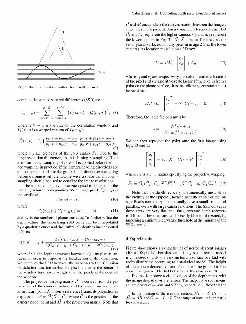
In order to avoid these problems and perform the correla-tion efficiently, we adopt a slicing algorithm. The main ideais to use a set of virtual planar surfaces slicing through theterrain as shown in Fig. 3. A similar concept was used byCollins [2] to perform matching between features extractedfrom the images. See also [12].

The virtual planar surfaces are similar in concept tohoropter surfaces [1] in stereo. For every planar surface k,if a terrain surface patch lies on the planar surface, then thereexists a projective warping �Pk between the two images for thispatch. If we designate the first image I1(x, y) and the secondimage I2(x, y), then for every virtual planar surface, we can

Yalin Xiong et al.: Computing depth maps from descent images

I

I2

1

Terrain

Fig. 3. The terrain is sliced with virtual parallel planes

compute the sum of squared differences (SSD) as:

Ck(x, y) =x+W∑

m=x−W

y+W∑n=y−W

(I1(m, n) − Ik

2 (m, n))2

, (8)

where 2W + 1 is the size of the correlation window andIk2 (x, y) is a warped version of I2(x, y):

Ik2 (x, y) = I2

(p00x + p01y + p02

p20x + p21y + p22,p10x + p11y + p12

p20x + p21y + p22

),

(9)where pij are elements of the 3×3 matrix �Pk. Due to thelarge resolution difference, an anti-aliasing resampling [5] ora uniform downsampling of I2(x, y) is applied before the im-age warping. In practice, if the camera heading directions arealmost perpendicular to the ground, a uniform downsamplingbefore warping is sufficient. Otherwise, a space-variant down-sampling should be used to equalize the image resolutions.

The estimated depth value at each pixel is the depth of theplane zk whose corresponding SSD image pixel Ck(x, y) isthe smallest:

z(x, y) = zk, (10)

whereCk(x, y) ≤ Cj(x, y), j = 1, . . . , M, (11)

and M is the number of planar surfaces. To further refine thedepth values, the underlying SSD curve can be interpolatedby a quadratic curve and the “subpixel” depth value computed[15] as:

z(x, y) = zk +δz(Ck+1(x, y) − Ck−1(x, y))

2(Ck+1(x, y) + Ck−1(x, y) − 2Ck(x, y)),

(12)where δz is the depth increment between adjacent planar sur-faces. In order to improve the localization of this operation,we compute the SSD between the windows with a Gaussianmodulation function so that the pixels closer to the center ofthe window have more weight than the pixels at the edge ofthe window.

The projective warping matrix �Pk is derived from the pa-rameters of the camera motion and the planar surfaces. Foran arbitrary point �X in some reference frame, its projection isexpressed as �x = �M( �X − �C), where �C is the position of thecamera nodal point and �M is the projection matrix. Note that

�C and �M encapsulate the camera motion between the images,since they are represented in a common reference frame. Let�C1 and �M1 represent the higher camera, �C2 and �M2 representthe lower camera in Fig. 3.1 �NT �X + zk = 0 represents theset of planar surfaces. For any pixel in image 2 (i.e., the lowercamera), its location must lie on a 3D ray:

�X = s �M−12

c2

r21

+ �C2, (13)

where c2 and r2 are, respectively, the column and row locationof the pixel and s is a positive scale factor. If the pixel is from apoint on the planar surface, then the following constraint mustbe satisfied:

s �NT �M−12

c2

r21

+ �NT �C2 + zk = 0. (14)

Therefore, the scale factor s must be

s = −�NT �C2 + zk

�NT �M−12 [c2, r2, 1]T

. (15)

We can then reproject the point onto the first image usingEqs. 13 and 15:

x1

y1z1

= �M1( �X − �C1) = �Pk

c2

r21

, (16)

where �Pk is a 3×3 matrix specifying the projective warping:

�Pk = �M1(�C2− �C1) �NT �M−12 −( �NT �C2+zk) �M1 �M−1

2 . (17)

Note that the depth recovery is numerically unstable inthe vicinity of the epipoles, located near the center of the im-age. Pixels near the epipoles usually have a small amount ofparallax, even with large camera motions. The SSD curves inthese areas are very flat, and, thus, accurate depth recoveryis difficult. These regions can be easily filtered, if desired, byimposing a minimum curvature threshold at the minima of theSSD curves.

4 Experiments

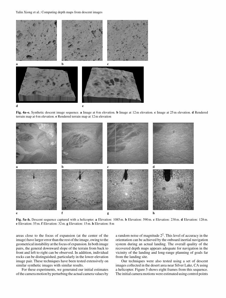
Figure 4a–c shows a synthetic set of nested descent images(400×400 pixels). For this set of images, the terrain modelis composed of a slowly varying terrain surface overlaid withrocks distributed according to a statistical model. The heightof the camera decreases from 25 m above the ground to 6 mabove the ground. The field of view of the camera is 70◦.

Figures 4d,e show a visualization of the depth maps, withthe image draped over the terrain. The maps have root-mean-square errors of 4.6 cm and 9.7 cm, respectively. Note that the

1 In the notation of the previous section, �M1 = �A, �C1 = 0,�M2 = �AR, and �C1 = −R−1T . The change of notation is primarily

for convenience.

Yalin Xiong et al.: Computing depth maps from descent images

a b c

d e

Fig. 4a–e. Synthetic descent image sequence. a Image at 6 m elevation. b Image at 12 m elevation. c Image at 25 m elevation. d Renderedterrain map at 6 m elevation. e Rendered terrain map at 12 m elevation

a b c d

e f g h

Fig. 5a–h. Descent sequence captured with a helicopter. a Elevation: 1085 m. b Elevation: 590 m. c Elevation: 238 m. d Elevation: 128 m.e Elevation: 55 m. f Elevation: 32 m. g Elevation: 15 m. h Elevation: 8 m

areas close to the focus of expansion (at the center of theimage) have larger error than the rest of the image, owing to thegeometrical instability at the focus of expansion. In both imagepairs, the general downward slope of the terrain from back tofront and left to right can be observed. In addition, individualrocks can be distinguished, particularly in the lower-elevationimage pair. These techniques have been tested extensively onsimilar synthetic images with similar results.

For these experiments, we generated our initial estimatesof the camera motion by perturbing the actual camera values by

a random noise of magnitude 2◦. This level of accuracy in theorientation can be achieved by the onboard inertial navigationsystem during an actual landing. The overall quality of therecovered depth maps appears adequate for navigation in thevicinity of the landing and long-range planning of goals farfrom the landing site.

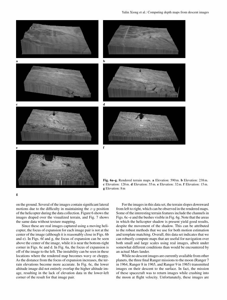
Our techniques were also tested using a set of descentimages collected in the desert area near Silver Lake, CA usinga helicopter. Figure 5 shows eight frames from this sequence.The initial camera motions were estimated using control points

Yalin Xiong et al.: Computing depth maps from descent images

a b

c d

e f

Fig. 6a–g. Rendered terrain maps. a Elevation: 590 m. b Elevation: 238 m.c Elevation: 128 m. d Elevation: 55 m. e Elevation: 32 m. f Elevation: 15 m.g Elevation: 8 m

g

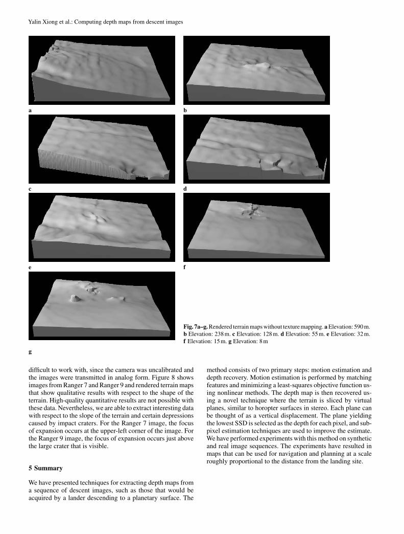
on the ground. Several of the images contain significant lateralmotions due to the difficulty in maintaining the x-y positionof the helicopter during the data collection. Figure 6 shows theimages draped over the visualized terrain, and Fig. 7 showsthe same data without texture mapping.

Since these are real images captured using a moving heli-copter, the focus of expansion for each image pair is not at thecenter of the image (although it is reasonably close in Figs. 6band e). In Figs. 6f and g, the focus of expansion can be seenabove the center of the image, while it is near the bottom-rightcorner in Figs. 6c and d. In Fig. 6a, the focus of expansion isoff of the image to the left. The instability can be seen in theselocations where the rendered map becomes wavy or choppy.As the distance from the focus of expansion increases, the ter-rain elevations become more accurate. In Fig. 6c, the loweraltitude image did not entirely overlap the higher altitude im-age, resulting in the lack of elevation data in the lower-leftcorner of the result for that image pair.

For the images in this data set, the terrain slopes downwardfrom left to right, which can be observed in the rendered maps.Some of the interesting terrain features include the channels inFigs. 6c–e and the bushes visible in Fig. 6g. Note that the areasin which the helicopter shadow is present yield good results,despite the movement of the shadow. This can be attributedto the robust methods that we use for both motion estimationand template matching. Overall, this data set indicates that wecan robustly compute maps that are useful for navigation overboth small and large scales using real images, albeit undersomewhat different conditions than would be encountered byan actual Mars lander.

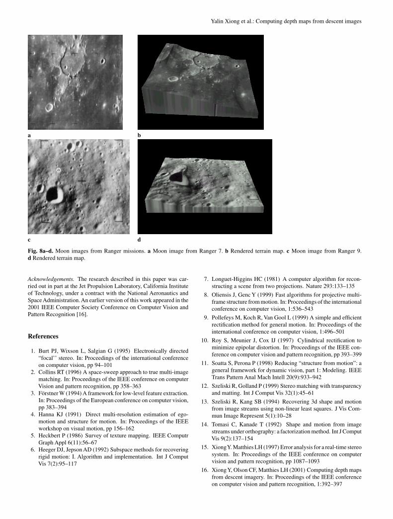
While no descent images are currently available from otherplanets, the three final Ranger missions to the moon (Ranger 7in 1964, Ranger 8 in 1965, and Ranger 9 in 1965) transmittedimages on their descent to the surface. In fact, the missionof these spacecraft was to return images while crashing intothe moon at flight velocity. Unfortunately, these images are

Yalin Xiong et al.: Computing depth maps from descent images

a b

c d

e f

Fig. 7a–g. Rendered terrain maps without texture mapping. a Elevation: 590 m.b Elevation: 238 m. c Elevation: 128 m. d Elevation: 55 m. e Elevation: 32 m.f Elevation: 15 m. g Elevation: 8 m

g

difficult to work with, since the camera was uncalibrated andthe images were transmitted in analog form. Figure 8 showsimages from Ranger 7 and Ranger 9 and rendered terrain mapsthat show qualitative results with respect to the shape of theterrain. High-quality quantitative results are not possible withthese data. Nevertheless, we are able to extract interesting datawith respect to the slope of the terrain and certain depressionscaused by impact craters. For the Ranger 7 image, the focusof expansion occurs at the upper-left corner of the image. Forthe Ranger 9 image, the focus of expansion occurs just abovethe large crater that is visible.

5 Summary

We have presented techniques for extracting depth maps froma sequence of descent images, such as those that would beacquired by a lander descending to a planetary surface. The

method consists of two primary steps: motion estimation anddepth recovery. Motion estimation is performed by matchingfeatures and minimizing a least-squares objective function us-ing nonlinear methods. The depth map is then recovered us-ing a novel technique where the terrain is sliced by virtualplanes, similar to horopter surfaces in stereo. Each plane canbe thought of as a vertical displacement. The plane yieldingthe lowest SSD is selected as the depth for each pixel, and sub-pixel estimation techniques are used to improve the estimate.We have performed experiments with this method on syntheticand real image sequences. The experiments have resulted inmaps that can be used for navigation and planning at a scaleroughly proportional to the distance from the landing site.

Yalin Xiong et al.: Computing depth maps from descent images

a b

c d

Fig. 8a–d. Moon images from Ranger missions. a Moon image from Ranger 7. b Rendered terrain map. c Moon image from Ranger 9.d Rendered terrain map.

Acknowledgements. The research described in this paper was car-ried out in part at the Jet Propulsion Laboratory, California Instituteof Technology, under a contract with the National Aeronautics andSpace Administration. An earlier version of this work appeared in the2001 IEEE Computer Society Conference on Computer Vision andPattern Recognition [16].

References

1. Burt PJ, Wixson L, Salgian G (1995) Electronically directed“focal’’ stereo. In: Proceedings of the international conferenceon computer vision, pp 94–101

2. Collins RT (1996) A space-sweep approach to true multi-imagematching. In: Proceedings of the IEEE conference on computerVision and pattern recognition, pp 358–363

3. Forstner W (1994) A framework for low-level feature extraction.In: Proceedings of the European conference on computer vision,pp 383–394

4. Hanna KJ (1991) Direct multi-resolution estimation of ego-motion and structure for motion. In: Proceedings of the IEEEworkshop on visual motion, pp 156–162

5. Heckbert P (1986) Survey of texture mapping. IEEE ComputrGraph Appl 6(11):56–67

6. Heeger DJ, Jepson AD (1992) Subspace methods for recoveringrigid motion: I. Algorithm and implementation. Int J ComputVis 7(2):95–117

7. Longuet-Higgins HC (1981) A computer algorithm for recon-structing a scene from two projections. Nature 293:133–135

8. Oliensis J, Genc Y (1999) Fast algorithms for projective multi-frame structure from motion. In: Proceedings of the internationalconference on computer vision, 1:536–543

9. Pollefeys M, Koch R, Van Gool L (1999) A simple and efficientrectification method for general motion. In: Proceedings of theinternational conference on computer vision, 1:496–501

10. Roy S, Meunier J, Cox IJ (1997) Cylindrical rectification tominimize epipolar distortion. In: Proceedings of the IEEE con-ference on computer vision and pattern recognition, pp 393–399

11. Soatta S, Perona P (1998) Reducing “structure from motion”: ageneral framework for dynamic vision, part 1: Modeling. IEEETrans Pattern Anal Mach Intell 20(9):933–942

12. Szeliski R, Golland P (1999) Stereo matching with transparencyand matting. Int J Comput Vis 32(1):45–61

13. Szeliski R, Kang SB (1994) Recovering 3d shape and motionfrom image streams using non-linear least squares. J Vis Com-mun Image Represent 5(1):10–28

14. Tomasi C, Kanade T (1992) Shape and motion from imagestreams under orthography: a factorization method. Int J ComputVis 9(2):137–154

15. XiongY. Matthies LH (1997) Error analysis for a real-time stereosystem. In: Proceedings of the IEEE conference on computervision and pattern recognition, pp 1087–1093

16. XiongY, Olson CF, Matthies LH (2001) Computing depth mapsfrom descent imagery. In: Proceedings of the IEEE conferenceon computer vision and pattern recognition, 1:392–397

Yalin Xiong et al.: Computing depth maps from descent images

Yalin Xiong is Director of Engineering in RAPID division of KLA-Tencor, specializing in image processing and computer vision al-gorithms for semiconductor inspection equipments. Prior to joiningKLA-Tencor, he was a senior staff in Jet Propulsion Lab, Caltechfrom 1998 to 2000, and senior engineer in Apple Computer from1996 to 1998. Dr. Yalin Xiong got Ph.D. from the Robotics Insti-tute of Carnegie Mellon University, and B.S. from the University ofScience and Technology of China.

Clark F. Olson received the B. S. degreein computer engineering in 1989 and theM.S. degree in electrical engineering in1990, both from the University of Wash-ington, Seattle. He received the Ph. D. de-gree in computer science in 1994 from theUniversity of California, Berkeley. Afterspending two years doing research at Cor-nell University, he moved to the Jet Propul-sion Laboratory, where he spent five yearsworking on computer vision techniquesfor Mars rovers and other applications. Dr.

Olson joined the faculty at the University of Washington, Bothell in2001. His research interestes include computer vision and mobilerobotics. He teaches classes on mathematical principles of comput-ing, database systems, and computer vision. He continues to workwith NASA/JPL on computer vision techniques for Mars exploration.

Larry H. Matthies PhD, computer sci-ence, Carnegie Mellon University, 1989;Supervisor, Machine Vision Group, JetPropulsion Laboratory (JPL). Dr. Matthieshas 21 years experience in developing per-ception systems for autonomous naviga-tion of robotic ground and air vehicles.He pioneered the development of real-timestereo vision algorithms for range imag-ing and accurate visual odometry in the1980’s and early 1990’s. These algorithmswill be used for obstacle detection onboard

the Mars Exploration Rovers (MER). The GESTALT system for ob-stacle avoidance for the MER rovers was developed in his group;this system is also currently the baseline for onboard obstacle de-tection for the 2009 Mars Science Laboratory (MSL) mission. Hisstereo vision-based range imaging algorithms were used for groundoperations by the Mars Pathfinder mission in 1997 to map terrainwith stereo imagery from the lander for planning daily operationsfor the Sojourner rover. He initiated the development at JPL of com-puter vision te s for autonomous safe landing and landing hazardavoidance for missions to Mars, asteroids, and comets. His groupdeveloped the Descent Image Motion Estimation System (DIMES)that will be used to estimate horizontal velocity of the MER landersduring terminal descent. Algorithms developed in his group for on-board crater recognition have been selected as the backup approachto regional hazard avoidance for the MSL mission. He also conductsresearch on terrain classification with a wide variety of sensors foroff-road navigation on Earth. He was awarded the NASA ExceptionalAchievement Medal in 2001 for his contributions to computer visionfor space missions. He is anAdjunctAssistant Professor of ComputerScience at the University of Southern California.