Computing Bifurcation Diagrams with

Deflation

�Casper Beentjes

St. Catherine’s College

University of Oxford

A thesis submitted for the degree of

M.Sc. in Mathematical Modelling and Scientific Computing

Trinity 2015

I would like to dedicate this thesis to all my friends and family who gaveme the space to grow up blissfully, but stay young in mind.

All grown-ups were once children. . .but only few of them remember it.

Antoine de Saint-Exupery (1900-1944)

Acknowledgements

This year has not been a solo-project and as a result I am indebted tomany people. However, after this intense year in Oxford and meetingnumerous fantastic people there is a risk of forgetting someone, know thatyour aid is acknowledged nonetheless!

First of all I would like to express my deepest gratitude to Dr. PatrickFarrell for his guidance in this thesis through good and bad times, hisenthusiasm in supervising and above all for being a great teacher. Aspecial thank you goes to Dr. Kathryn Gillow for her never-ending supportas our course-director. Furthermore I would like to thank Jack, Stephenand my MMSC-cohort for this amazing year. You all kept me sane, inand outside the Mathematical Institute, and made me feel at home. Inparticular, I would like to thank Markus, Matteo and Tori for their helpfuldiscussions over the past year and especially whilst writing this thesis.

Lastly, I am extremely grateful for the funding received from VSBfonds,Genootschap Noorthey and Stichting dr. Hendrik Muller’s VaderlandschFonds. Without their combined generous help this year in Oxford wouldnot have been possible.

If our small minds, for some convenience, divide this glass of wine, this

universe, into parts – physics, biology, geology, astronomy, psychology,

and so on – remember that nature does not know it!

So let us put it all back together, not forgetting ultimately what it is for.

Let it give us one more final pleasure: drink it and forget it all!

Richard Feynman (1918-1988)

Abstract

One of the main deficiencies of current methods in numerical bifurca-tion analysis is their inability to detect solution branches without firstlocating a bifurcation point. As a result these methods cannot computedisconnected bifurcation branches, or branches that connect outside ofthe parameter domain of study. Furthermore, the detection techniquesfor bifurcation points are not problem-scale invariant. As a result the costof computing bifurcation points in large-scale systems is often a prohibit-ing factor in the computation of bifurcation diagrams. In this thesis wepropose a method to overcome these two issues.

We study the use of deflation techniques combined with Newton’s methodto generate multiple solution branches starting from a single initial solu-tion. A theoretical framework for root-convergence and deflation of func-tions in Banach spaces is set up. In this framework we derive the firstsufficient conditions for convergence towards multiple solutions if New-ton’s method and deflation are combined.

Deflation can be made a scalable technique and as a result could be usedin tracing out bifurcation diagrams for large-scale systems. We comparearclength continuation augmented with deflation as a method to computebifurcation diagrams with AUTO-07P, one of the most used and reliablenumerical bifurcation software packages available. We find that for a rangeof illustrative problems AUTO-07P fails to compute complete bifurcationdiagrams, whereas deflation and continuation combined yield an accurateresult.

Note: this digital version contains modifications made to the paper versionthat has been submitted to the Examination Schools on 3 September 2015.

Contents

1 Introduction 11.1 Outline of work . . . . . . . . . . . . . . . . . . . . . . . . . . . . . . 4

2 Background on Newton’s method and deflation 62.1 Newton’s method . . . . . . . . . . . . . . . . . . . . . . . . . . . . . 62.2 Deflation techniques . . . . . . . . . . . . . . . . . . . . . . . . . . . 7

2.2.1 Wilkinson deflation of polynomials . . . . . . . . . . . . . . . 72.2.2 General deflation in Banach space setting . . . . . . . . . . . . 9

3 A review of local convergence theorems for Newton’s method 113.1 Classical theorems . . . . . . . . . . . . . . . . . . . . . . . . . . . . 113.2 Affine covariant theorems . . . . . . . . . . . . . . . . . . . . . . . . . 173.3 Convergence theorems for analytic functions . . . . . . . . . . . . . . 203.4 Summary of local convergence theorems . . . . . . . . . . . . . . . . 26

4 Local convergence of Newton’s method and deflation 274.1 Examples of local convergence to multiple solutions . . . . . . . . . . 274.2 Convergence criteria for deflated functions . . . . . . . . . . . . . . . 30

4.2.1 Deflation on analytic functions . . . . . . . . . . . . . . . . . . 304.2.2 Deflation on general functions . . . . . . . . . . . . . . . . . . 33

5 Bifurcation diagrams and deflation 365.1 Numerical bifurcation techniques . . . . . . . . . . . . . . . . . . . . 365.2 Deflation and continuation combined . . . . . . . . . . . . . . . . . . 395.3 Comparison with existing software . . . . . . . . . . . . . . . . . . . 40

5.3.1 Steady state continuation . . . . . . . . . . . . . . . . . . . . 41

6 Conclusions 48

A Proofs of auxiliary results 50A.1 Proof of Lemma 1 . . . . . . . . . . . . . . . . . . . . . . . . . . . . . 50A.2 Proof of Lemma 7 . . . . . . . . . . . . . . . . . . . . . . . . . . . . . 51

Bibliography 52

i

List of notation

N,R,R+,C Natural, real, positive real and complex numbers respectively.

<(x),=(x) Real and imaginary part of x.

X, Y, Z General Banach spaces.

B(x, ρ), B(x, ρ) Open, respectively closed, ball centred around x with radius ρ.

L(X, Y ) Set of bounded linear operators from X to Y .

GL(X, Y ) Set of invertible linear operators from X to Y .

I Identity operator (from X to X).

F ′(x) Frechet derivative of F (x).

Fx(x, y) Partial Frechet derivative of F (x, y) with respect to x.

ii

1. Introduction

As pointed out by the acclaimed physicist Eugene Wigner in his lecture “The unrea-sonable effectiveness of mathematics in the natural sciences” [47], mathematics turnsup in seemingly unexpected situations and is often remarkably capable of graspingcomplex structures hidden beneath our observations of nature. One might thereforeconsider mathematics as the lingua franca among scientists as it provides a universallanguage able to lift physical problems into the realm of mathematical abstraction.

For many physical problems the result of this abstraction is a mathematical modelwhich can be described by a set of equations. For this thesis we start with a verygeneral setting, where the equations are given by

F (u, λ) = 0. (1.1)

Without specifying the exact form of the equations F we do make a clear distinctionbetween the roles of u and λ. We let u denote the general set of variables and λthe set of problem parameters. This difference between the two can be hard to pindown, but for most purposes we think of the variables as the measurable outcome ofan experiment whereas the parameters, also called controls, govern the set-up of theexperiment. One could thus say that u and λ constitute the output and input of themodel respectively. Consider as a simple example the problem of the deformation ofa (slender) beam under a load, see Figure 1.1. The deflection of the beam is now avariable of the problem and the external load is part of the set of control parameters.

λ

(a) Undeformed beam

λu

(b) Deformed beam

Figure 1.1: Deformation of a horizontal placed beam due to a vertical load λ.

A natural question to ask is how the output of the model, the displacement,changes if we alter one of the parameters, in this case the load λ. The reader canexperimentally verify the rather uninteresting result that increasing the load increasesthe bending of the beam. There might be, however, a point at which the beam cannotsustain any additional small weight any longer, resulting in failure of the beam, thestraw that breaks the camel’s back. Here we see an example of a problem where agradual change in the parameter can lead to a drastic change in the behaviour of itsvariables.

A less dramatic result is observed when we place the beam vertically and put aload on top of the beam, see Figure 1.2. Initially slowly increasing the load will notresult in any bending of the beam; it will merely compress the beam in the verticaldirection. There is, however, a critical value of the parameter λc which induces alarge out of plane deformation of the beam, known as buckling.

These are examples where smoothly passing a parameter threshold value resultsin a qualitatively different solution, a phenomenon known as a bifurcation. A wide

1

λ

(a) Undeformed beam

λ

(b) Deformed beam with λ < λc

λ λ

(c) Deformed beam with λ > λc

Figure 1.2: Deformation of a vertically placed beam due to a vertical load λ. Theresulting deformation changes qualitatively around a critical value λc of the controlparameter.

variety of bifurcation types exist, such as the creation or annihilation of a solution, thesudden appearance of periodic cycles or the change in stability of a solution, i.e. theresponse of the solution to small perturbations. For a more (mathematically) completediscussion see [3]. As the concept of a bifurcation is very general it appears in awide range of applications ranging from continuum mechanics to ecological problems.Examples being pattern formation in chemical and biological systems, buckling ofbeams and structures, transitions in fluid flows such as the classical Taylor-Couetteexperiment, and (possibly) the Tacoma Narrows bridge collapse [43]. In engineeringscience bifurcations are widely studied as they potentially can induce catastrophicfailure of structures.

A common way to visualise bifurcations is by means of a bifurcation diagram, inwhich we plot J(u), a scalar measure of the outcome u, as a function of the parametersλ. This way we can depict the structure of the solution curves in parameter space,which are known as solution branches, and their interactions at bifurcation points.See Figure 1.3 for sketches of bifurcation diagrams.

The analysis of the solution behaviour of (1.1) as a function of the parameterset λ and the construction of an accompanying bifurcation diagram is, however, of-ten difficult as the systems of equations for which bifurcations occur are necessarilyof non-linear nature. One of the ways to nonetheless investigate the behaviour ofthese systems is by use of numerical methods, i.e. by numerically approximating theirsolutions.

In order to find a numerical solution to non-linear equations we typically useiterative methods. If we provide an initial guess of the root of (1.1) then thesemethods try on every iteration to find a better approximation to the root. One ofthe most popular methods in the class of iterative methods is Newton’s method,due to its fast convergence properties close to actual roots of the equation. Notethough that whereas starting close to a solution with Newton’s method (or any otheriterative method) can result in rapid convergence, starting just slightly too far away

2

λcλ

J(u

)

(a) Connected branches

λcλ

J(u

)

(b) Disconnected branches

Figure 1.3: Schematic bifurcation diagrams showing a scalar measure J(u) of theoutput u as a function of the parameter λ. Bifurcation points are denoted by • andare located at λc and λc respectively. Although the diagrams bear a resemblanceto each other the solution branch structure is fundamentally different in terms ofconnectedness.

could result in extremely fast divergence, especially in the case of highly non-linearproblems.

Iterative methods provide us with the most basic framework for the computationof bifurcation diagrams, numerical continuation. If we are given an initial point onour solution branch we can use this point as an initial guess to compute a solutionon the same solution branch for a different parameter value using iterative methodsand thus continue our solution along a branch. If we take small enough steps so thatthe iterative methods will converge on each step we can proceed iteratively alongbranches and thus trace out full solution branches.

To illustrate the working of numerical bifurcation algorithms let us look at thebifurcation diagrams in Figure 1.3. Suppose we start off in the left part of the bifurca-tion diagrams and trace out the diagrams in the positive λ-direction. Most numericalbifurcation algorithms are able to correctly trace out the black solution branch inFigure 1.3 by making use of continuation techniques. Having found this one solutionbranch the next question becomes: how can we detect and trace out the red branches?

In the case of Figure 1.3a we encounter a bifurcation point on this curve and wemight detect this using numerical bifurcation techniques, see for example [44]. Havingfound this special point we ideally want to be able to switch to the red branches inorder to fully trace out the diagram. In order to do so we recall that iterative methodsneed to be started with sufficiently good initial guesses in order to yield convergence.Various techniques, based on results in bifurcation theory, exist to construct initialguesses for the red branches close to the bifurcation point. These are implementedin contemporary numerical bifurcation software packages and allow users to switchbranches if the location of the bifurcation point is known, see for instance [28]. Currentbifurcation algorithms are therefore able to successfully trace out Figure 1.3a.

3

The case of disconnected branches as in Figure 1.3b on the other hand oftenposes a more severe problem. First of all if one does not know beforehand that adisconnected branch of solutions exists it is likely that it will remain hidden in thecourse of the construction of the bifurcation diagram as we do not find a bifurcationpoint on the branch, which was our indicator in Figure 1.3a for multiple solutions.Even if we do know that extra branches of solutions for fixed λ exist the questionstill remains; how can we construct an initial solution on this other branch whichwould allow us to follow this branch using continuation? Standard branch switchingtechniques cannot be applied now as we have not located a bifurcation point whichis needed for the standard methods to work. This leaves bifurcation diagrams likeFigure 1.3b uncomputable by current numerical bifurcation algorithms.

We are thus left in the situation where multiple solutions to (1.1) for fixed λ existbut we are not able to locate a bifurcation point which prevents us from calculat-ing the full bifurcation diagram. This gives rise to the question: can we devise anumerical technique that is able not only to find a solution, but also, if they exist,to find multiple solutions? One such technique has been known for some decades towork, but only for a special class of functions, namely scalar polynomials. Wilkinsonconsidered a technique, now known as deflation, to find multiple roots of polynomialsstarting from a single initial guess [48]. Based on work by Brown and Gearhart [8]this deflation technique was recently generalised by Farrell, Birkisson and Funke [18],to apply to a more general class of functions, which provides a possible solution to theproblem sketched in Figure 1.3b. In this thesis we will investigate the use of defla-tion in robustly tracing out bifurcation diagrams, especially those with disconnectedbranches. In particular, we combine deflation for fixed parameters to generate multi-ple solutions on distinct solution branches with standard continuation techniques totrace out branches, which allows us to find more complete bifurcation diagrams.

1.1 Outline of work

The work in this thesis can be roughly divided in two; a theoretical section and amore practical, numerical section, which are linked together by the main idea of thethesis, the deflation technique.

First in the the theoretical part we will try to answer the question of whether wecan derive sufficient conditions for the deflation method in combination with Newton’smethod to converge to multiple solutions if they exist. In order to achieve this wewill start with background material on Newton’s method and deflation techniques.To incorporate a wide range of applications we look at functions F : X → Y , where Xand Y are Banach spaces. This allows us to discuss a very general class of problemsthat are of interest to the scientific community, namely that of partial differentialequations (PDEs), ordinary differential equations (ODEs), integral equations andalgebraic problems. We will for sake of notation consider X = U × Λ, a product ofthe space of variables U and that of parameters Λ.

We first prove a new result on the convergence of Wilkinson deflation on scalarpolynomials with real roots, which shows that indeed sufficient conditions can be

4

found in this special case. In order to derive more general sufficient conditions forconvergence of deflation to multiple roots we review the (local) convergence theoryavailable for Newton’s method in Banach space setting. We bring together some welland lesser known convergence theorems and their proofs and look at their similaritiesand differences. No such review has been published before.

Next we prove the novel result that under certain restrictions on the type of defla-tion, some local Newton convergence theorems are still applicable after our functionhas been deflated. These results then allow us to start the derivation of sufficientconditions for convergence towards multiple solutions of the deflation technique inBanach spaces.

The final chapter looks at a practical numerical bifurcation algorithm built on thedeflation technique. In this chapter we will show that certain types of problems whichwere previously inaccessible by traditional implementations of numerical bifurcationtechniques, such as disconnected branches, can be tackled with the addition of de-flation. We will benchmark our implementation for some illustrative problems withone of the most robust and reliable numerical bifurcation software packages available,AUTO-07P [15]. We find that our algorithm succeeds in cases where the methods inAUTO-07P fail, demonstrating the power of the approach.

5

2. Background on Newton’s methodand deflation

For this thesis we will look atF (u, λ) = 0, (2.1)

in the general setting of Banach spaces so that its theory can be applied to a widevariety of problems, including ODEs and PDEs. In order to simplify notation, let theBanach spaces of the variables and parameters be denoted by U and Λ respectivelyand let X = U × Λ be their product space.

In order to study (2.1) we can therefore consider X and Y general Banach spacesand F : X → Y . Solving (2.1) now translates to finding the roots of F , i.e. x ∈ Xthat satisfy F (x) = 0, which can now be amongst other things scalar solutions toalgebraic problems or functions solving a differential equation.

First we will introduce a common technique, Newton’s method, to approximatea solution to F (x) = 0. This method is only concerned with finding a single rootto this equation. There are, however, functions F for which multiple roots do exist.Particularly of interest to us is the problem of detection of multiple branches in theconstruction of bifurcation diagrams. A natural question thus is whether there existmethods to find more than one root. To this end we will introduce one computationaltechnique, deflation, which can make, under certain conditions, Newton’s method findmultiple roots starting from just one initial guess.

2.1 Newton’s method

Exact solutions to the root-finding problem are often hard to acquire. One can,however, try to approximate the roots by means of various schemes. A popular classof approximation schemes uses an iterative method of the form,

xk+1 = xk + ∆xk, (2.2)

where the update ∆xk depends on the type of iterative method. Starting from an ini-tial point x0 one hopes to produce a sequence by the iterative method which convergestowards a root of F .

A specific and widely studied iterative method is Newton’s method, or the Newton-Raphson method. The classical version of Newton’s method defines the updates bythe equation

F ′(xk)∆xk = −F (xk), (2.3)

where F ′(x) denotes the Frechet derivative of F (x), which we have to assume to existin order for Newton’s method to be well-defined. One motivation for this specific formof the update can be found by looking at the local Taylor expansion of F around thecurrent iterate xk.

6

Affine transformation invariance

An important observation about Newton’s method is its behaviour under affine trans-formations of the domain or codomain of the function F . If A ∈ GL(Y ), then onecan see from (2.3) that the functions F (x) and AF (x) yield exactly the same New-ton sequence, i.e. Newton’s method is affine covariant. Furthermore we see that ifB ∈ GL(X), then the functions F (x) and G(y) = F (By) yield Newton sequences {xk}and {yk} that are simply related by a scaling xk = Byk. Newton’s method is thussaid to be affine contravariant as well. These properties have important implications,as we will see later on.

2.2 Deflation techniques

The aforementioned Newton’s method can compute approximate roots starting froman initial guess x0. If we are to find multiple solutions starting from x0 we will have toextend our method and one possible candidate to do so is deflation. To introduce thegeneral technique of deflation we first consider a specific type of deflation which canbe applied to find the roots of scalar polynomials, now known as Wilkinson deflation,which was the first deflation technique developed [48].

2.2.1 Wilkinson deflation of polynomials

Suppose we are given a scalar polynomial p with distinct roots r1, · · · , rN ∈ C so thatwe can write p(x) =

∏Ni=1(x− ri). If by some method we have acquired a set of roots

with indices i ∈ S then we can attempt to find the unknown roots by our originalmethod if we can hide the known roots from our root-finder. In the case of scalarpolynomials this can be achieved by considering a deflated polynomial

q(x) =p(x)∏

i∈S(x− ri), (2.4)

where we have now filtered the known roots from the original polynomial by polyno-mial division. Applying our root-finding technique of choice to this deflated polyno-mial will, if it converges, converge to a root which has not yet been found.

The practical implementation of this technique has to overcome several issues dueto the ill-conditioning of the root-finding problem of polynomials and finite arithmetic,see for example [36, 48], but we will not explore this matter further here. Instead wewill now look at the combination of Wilkinson deflation with Newton’s method andshow that this combination can provably yield multiple roots starting from a singleinitial guess, a result which has not been published before.

Convexity & global convergence

If we have a polynomial with distinct real roots, then we can prove that there existinfinitely many points which will converge to all the roots of the polynomial by makinguse of local convexity of the polynomial. The rate of convergence is, however, not

7

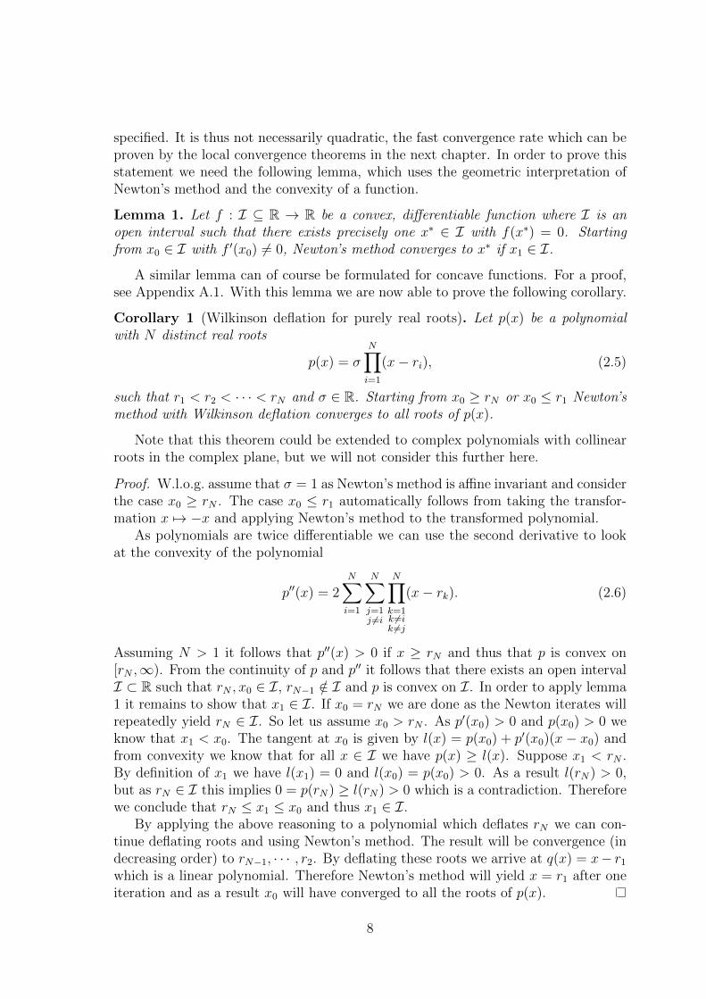
specified. It is thus not necessarily quadratic, the fast convergence rate which can beproven by the local convergence theorems in the next chapter. In order to prove thisstatement we need the following lemma, which uses the geometric interpretation ofNewton’s method and the convexity of a function.

Lemma 1. Let f : I ⊆ R → R be a convex, differentiable function where I is anopen interval such that there exists precisely one x∗ ∈ I with f(x∗) = 0. Startingfrom x0 ∈ I with f ′(x0) 6= 0, Newton’s method converges to x∗ if x1 ∈ I.

A similar lemma can of course be formulated for concave functions. For a proof,see Appendix A.1. With this lemma we are now able to prove the following corollary.

Corollary 1 (Wilkinson deflation for purely real roots). Let p(x) be a polynomialwith N distinct real roots

p(x) = σN∏i=1

(x− ri), (2.5)

such that r1 < r2 < · · · < rN and σ ∈ R. Starting from x0 ≥ rN or x0 ≤ r1 Newton’smethod with Wilkinson deflation converges to all roots of p(x).

Note that this theorem could be extended to complex polynomials with collinearroots in the complex plane, but we will not consider this further here.

Proof. W.l.o.g. assume that σ = 1 as Newton’s method is affine invariant and considerthe case x0 ≥ rN . The case x0 ≤ r1 automatically follows from taking the transfor-mation x 7→ −x and applying Newton’s method to the transformed polynomial.

As polynomials are twice differentiable we can use the second derivative to lookat the convexity of the polynomial

p′′(x) = 2N∑i=1

N∑j=1j 6=i

N∏k=1k 6=ik 6=j

(x− rk). (2.6)

Assuming N > 1 it follows that p′′(x) > 0 if x ≥ rN and thus that p is convex on[rN ,∞). From the continuity of p and p′′ it follows that there exists an open intervalI ⊂ R such that rN , x0 ∈ I, rN−1 /∈ I and p is convex on I. In order to apply lemma1 it remains to show that x1 ∈ I. If x0 = rN we are done as the Newton iterates willrepeatedly yield rN ∈ I. So let us assume x0 > rN . As p′(x0) > 0 and p(x0) > 0 weknow that x1 < x0. The tangent at x0 is given by l(x) = p(x0) + p′(x0)(x − x0) andfrom convexity we know that for all x ∈ I we have p(x) ≥ l(x). Suppose x1 < rN .By definition of x1 we have l(x1) = 0 and l(x0) = p(x0) > 0. As a result l(rN) > 0,but as rN ∈ I this implies 0 = p(rN) ≥ l(rN) > 0 which is a contradiction. Thereforewe conclude that rN ≤ x1 ≤ x0 and thus x1 ∈ I.

By applying the above reasoning to a polynomial which deflates rN we can con-tinue deflating roots and using Newton’s method. The result will be convergence (indecreasing order) to rN−1, · · · , r2. By deflating these roots we arrive at q(x) = x− r1

which is a linear polynomial. Therefore Newton’s method will yield x = r1 after oneiteration and as a result x0 will have converged to all the roots of p(x).

8

Note that this theorem implies that there are indeed functions which allow one tofind multiple roots starting from a fixed x0, but the class of functions is unfortunatelyrather limited and the theorem does not have a natural extension into the more generalBanach space setting. Therefore we will now look at a generalisation of Wilkinsondeflation which is applicable in Banach space setting.

2.2.2 General deflation in Banach space setting

Instead of considering a scalar polynomial we return to the problem of a general(non-linear) function F : X → Y , where X and Y are Banach spaces. Brown andGearhart [8] generalised the technique of Wilkinson deflation for the case where X andY are finite dimensional real or complex vector spaces, say Rn or Cn, by consideringdeflation matrices of the form

M(x; r) =A

‖x− r‖, (2.7)

where A is a non-singular matrix. This concept of deflation matrices has a naturalextension to our previous framework of general Banach spaces, as was set out byFarrell, Birkisson and Funke [18].

Definition 1 (Deflation operator on a Banach space [6]). Let X, Y and Z be Banachspaces, and D ⊆ X be an open subset. Let F : D ⊂ X → Y be a Frechet differentiableoperator with derivative F ′. For each r ∈ D, let M(·; r) :D\{r} → GL(Y, Z). Wesay that M is a deflation operator if for any F such that F (r) = 0 and F ′(r) isnonsingular, we have

lim infi→∞

||M(xi; r)F (xi)|| > 0 (2.8)

for any sequence {xi} converging to r, xi ∈ D \ {r}.

The most common and practical case is where the deflation operator is a linearoperator in GL(Y ). For this thesis we will use a generalisation of the deflationmatrices by Brown and Gearhart, namely the class of shifted deflation operators.

Definition 2 (Shifted deflation [18]). Shifted deflation specifies

Mp,α(x; r) =

(1

||x− r||p+ α

)I, (2.9)

where α ≥ 0 is the shift, p ≥ 1 and I is the identity operator on Y .

The shift and exponent parameter of the deflation operator can be chosen so as toimprove the convergence of the root-finding technique applied to the deflated function,see [18]. Note that any other A ∈ GL(Y ) can be chosen instead of I ∈ GL(Y ), butas Newton’s method is affine covariant this would not change the Newton sequences.

9

Convergence to multiple roots

The objective of our theoretical endeavour is to derive conditions which can guaranteeus to find multiple roots, starting from a single initial guess x0. Given an arbitraryinitial guess and function F then we are, however, not guaranteed to even find a singleapproximate root of F using Newton’s method. It is therefore of interest to see underwhat conditions we can establish guaranteed convergence of Newton’s method. Tothis end we present in the next chapter a review of various convergence theorems forthe classical version of Newton’s method as defined by (2.2,2.3).

These local convergence theorems will yield open neighbourhoods around roots ofthe function which form regions of guaranteed convergence. Given a region D ⊂ Xwith two roots x∗1 and x∗2 we can then sketch the general idea for a convergence resulttowards multiple roots. As deflation is changing the objective function we expectthese convergence regions to change and we therefore look for conditions in which theregions before and after deflation have a non-empty overlap for different roots, as inFigure 2.1, so that any point in this overlap will converge to at least two solutions.

x∗1

x∗2

x0ρ1

ρ2

D

(a) Convergence before deflation

x∗1

x∗2

x0

ρ′2

D

(b) Convergence after deflation

Figure 2.1: Illustration of local convergence regions around roots. The approach weare taking in deriving sufficient conditions for convergence of x0 towards multipleroots is sketched here. The initial guess x0 lies within a convergence region for x∗1initially. After deflation x0 will no longer converge to x∗1, but instead lies within anew region of convergence around x∗2, which has increased relative to the convergenceregion for the undeflated function.

10

3. A review of local convergence theoremsfor Newton’s method

Recall Newton’s method for finding approximate solutions to F (x) = 0

xk+1 = xk + ∆xk, (3.1a)

F ′(xk)∆xk = −F (xk), (3.1b)

which we need to initialise by an initial guess x0. We hope to get a Newton sequencewhich converges to a root of F , but as mentioned before Newton’s method is notguaranteed to succeed in doing so. Several sufficient conditions do exist which canguarantee convergence of a root if we start in a neighbourhood close to a root andwe present here a non-exhaustive review of various local convergence theorems forthe classical version of Newton’s method as defined by (3.1) in finding solutions toF (x) = 0.

Note that our general objective is finding sufficient conditions for convergence tomultiple solutions, an idea sketched in Figure 2.1, which we will keep in mind whilelooking at the different approaches of the theorems.

3.1 Classical theorems

As can be seen from (3.1) Newton’s method relies upon the solvability of a linear sys-tem involving the Frechet derivative of F at the current iterate. In order to guaranteea solution to the Newton update equation (3.1b) one often requires invertibility ofthis Frechet derivative. The following standard result from linear functional analysisgives sufficient conditions in order for a linear operator to be invertible.

Lemma 2 (Banach perturbation lemma). Let T : X → Y be a linear operator suchthat ‖T‖ < 1. Then I + T is invertible and

1

1 + ‖T‖≤ ‖(I + T )−1‖ ≤ 1

1− ‖T‖. (3.2)

For a proof, see, for example, [42, Theorem 4.40]. This will be a key result inthe following convergence theorems as it can be used to show that (3.1) has a well-defined solution. Another important result is the extension of the mean-value theoremto functions on Banach spaces.

Lemma 3 (Mean-value theorem). Let F : X → Y be a continuously Frechet differ-entiable operator on the open subset D ⊆ X. For any x, y ∈ D we have

F (x)− F (y) =

∫ 1

0

F ′(tx+ (1− t)y)(x− y) dt. (3.3)

11

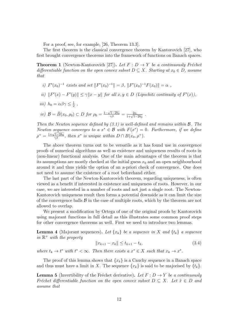
For a proof, see, for example, [26, Theorem 13.3].The first theorem is the classical convergence theorem by Kantorovich [27], who

first brought convergence theorems into the framework of functions on Banach spaces.

Theorem 1 (Newton-Kantorovich [27]). Let F : D → Y be a continuously Frechetdifferentiable function on the open convex subset D ⊆ X. Starting at x0 ∈ D, assumethat

i) F ′(x0)−1 exists and set ‖F ′(x0)−1‖ = β, ‖F ′(x0)−1F (x0)‖ = α ,

ii) ‖F ′(x)− F ′(y)‖ ≤ γ‖x− y‖ for all x, y ∈ D (Lipschitz continuity of F ′(x)),

iii) h0 = αβγ ≤ 12

,

iv) B = B(x0, ρ0) ⊂ D for ρ0 = 1−√

1−2h0γβ

= 2α1+√

1−2h0.

Then the Newton sequence defined by (3.1) is well-defined and remains within B. TheNewton sequence converges to a x∗ ∈ B with F (x∗) = 0. Furthermore, if we define

ρ+ = 1+√

1−2h0γβ

, then x∗ is unique within D ∩B(x0, ρ+).

The above theorem turns out to be versatile as it has found use in convergenceproofs of numerical algorithms as well as existence and uniqueness results of roots in(non-linear) functional analysis. One of the main advantages of the theorem is thatits assumptions are mostly checked at the initial guess x0 and an open neighbourhoodaround it and thus yields the option of an a-priori check of convergence. One doesnot need to assume the existence of a root beforehand either.

The last part of the Newton-Kantorovich theorem, regarding uniqueness, is oftenviewed as a benefit if interested in existence and uniqueness of roots. However, in ourcase, we are interested in a number of roots and not just a single root. The Newton-Kantorovich uniqueness result then forms a potential downside as it can limit the sizeof the convergence balls B in the case of multiple roots, which by the theorem are notallowed to overlap.

We present a modification by Ortega of one of the original proofs by Kantorovichusing majorant functions in full detail as this illustrates some common proof stepsfor other convergence theorems as well. First we need to introduce two lemmas.

Lemma 4 (Majorant sequences). Let {xk} be a sequence in X and {tk} a sequencein R+ with the property

‖xk+1 − xk‖ ≤ tk+1 − tk, (3.4)

where tk → t∗ with t∗ <∞. Then there exists a x∗ ∈ X such that xk → x∗.

The proof of this lemma shows that {xk} is a Cauchy sequence in a Banach spaceand thus must have a limit in X. The sequence {xk} is said to be majorised by {tk}.

Lemma 5 (Invertibility of the Frechet derivative). Let F : D → Y be a continuouslyFrechet differentiable function on the open convex subset D ⊆ X. Let x ∈ D andassume that

12

i) F ′(x)−1 exists and set ‖F ′(x)−1‖ = β,

ii) ‖F ′(x)− F ′(y)‖ ≤ γ‖x− y‖ for all x, y ∈ D (Lipschitz continuity of F ′(x)).

Then for all x ∈ B (x, 1/βγ) the Frechet derivative F ′(x) is invertible and its normis bounded by

‖F ′(x)−1‖ ≤ β

1− βγ‖x− x‖. (3.5)

Proof. If x ∈ B (x, 1/βγ) we find that G(x) = I − F ′(x)−1F ′(x) satisfies ‖G‖ < 1 byuse of the Lipschitz continuity of the Frechet derivative on D. By lemma 2 we thenknow that (I + G)−1 exists, i.e. (F ′(x)−1F ′(x))−1 is well-defined, which proves thatF ′(x)−1 exists. The bound on the norm follows from (3.2).

With these lemmas we can now give the proof by Ortega which constructs anexplicit majorant sequence to the Newton sequence to prove convergence.

Proof of Theorem 1 [34]. Observation 1 (Difference in Newton iterates)Given xk for k = 1, . . . , N and using lemma 5 we find that the difference between thenext iterates satisfies

‖xN+1 − xN‖ = ‖F ′(xN)−1F (xN)‖ (3.6)

≤ ‖F ′(xN)−1‖ ‖F (xN)‖ (3.7)

≤ β

1− βγ‖xN − x0‖‖F (xN)‖. (3.8)

To find an upper bound for the last term note that we can apply the mean-valuetheorem and then use convexity of D to apply the Lipschitz continuity

‖F (xN)‖ = ‖F (xN)− F (xN−1)− F ′(xN−1)(xN − xN−1)‖ (3.9)

= ‖∫ 1

0

[F ′(sxN + (1− s)xN−1)− F ′(xN−1)] ds (xN − xN−1)‖ (3.10)

≤∫ 1

0

‖F ′(sxN + (1− s)xN−1)− F ′(xN−1)‖ ds ‖xN − xN−1‖ (3.11)

≤ γ

2‖xN − xN−1‖2. (3.12)

Note that we have used (3.1) at step N − 1 in the first line.Observation 2 (Construction of an explicit majorant sequence)

Let φ(t) = βγ2t2 − t+ α. Note that this is a convex quadratic. By h0 ≤ 1/2 its roots,

given by ρ0 and ρ+, are real. Then applying Newton to this function will result in amonotonically converging sequence to the roots. If we start with t0 = 0 we will thuscreate a sequence {tk} such that tk ↑ ρ0 as ρ0 ≤ ρ+. This sequence is given by

tk+1 = tk −βγ2t2k − tk + α

βγtk − 1. (3.13)

13

Claim: {tk} is a majorising sequence for the Newton sequence started from x0. Notethat t1 = α and ‖x1 − x0‖ = ‖F ′(x0)−1F (x0)‖ = α. Now suppose that for allk = 0, 1, . . . N the Newton sequence is majorised, i.e. ‖xk − xk−1‖ ≤ tk − tk−1.

Then we find by observation 1 that the difference in Newton iterates is boundedby

‖xN+1 − xN‖ ≤βγ

2− 2βγ‖xN − x0‖‖xN − xN−1‖2 ≤ βγ/2

1− βγtN(tN − tN−1)2. (3.14)

Using the definition of the Newton sequence from φ(t) and

tk+1 =tk2

+tk2− α

βγtk − 1, (3.15)

we can deduce that the last term in (3.14) is equal to tN+1 − tN , which proves theclaim. Therefore there exists a x∗ ∈ D such that xk → x∗. Additionally we have that‖xN − x0‖ ≤

∑N−10 ‖xi+1 − xi‖ ≤ tN − t0 = tN ≤ ρ0 so that the Newton sequence

remains in B. Thus x∗ ∈ B, and from convergence of Newton’s method it follows thatF (x∗) = 0.If h0 < 1/2 we find that ρ0 < (βγ)−1 and thus from (3.14) that the convergence is infact quadratic by using that ‖xN − x0‖ ≤ ρ0.

Observation 3 (Uniqueness of solution)We define U = D∩B(x0, ρ

+) andH(x) = F ′(x0)−1F (x). Then H ′(x) = F ′(x0)−1F ′(x)and as a result H ′(x0) = I. Note that H is Lipschitz continuous on D as well withLipschitz constant βγ.

Suppose there exist a, b ∈ B(x0,1βγ

) such that F (a) = F (b) = 0, but a 6= b. Thenwe find

‖a− b‖ = ‖H(a)−H(b)− I(a− b)|| = ‖H(a)−H(b)−H ′(x0)(a− b)‖. (3.16)

By use of the mean value theorem we then find

‖a− b‖ ≤∫ 1

0

‖H ′(sa+ (1− s)b)−H ′(x0)‖ ds‖a− b‖ (3.17)

≤ sups∈[0,1]

‖H ′(sa+ (1− s)b)−H ′(x0)‖ ‖a− b‖ (3.18)

≤ βγ‖a− b‖ sups∈[0,1]

‖sa+ (1− s)b− x0‖ (3.19)

= βγ‖a− b‖ sups∈[0,1]

‖s(a− x0) + (1− s)(b− x0)‖ (3.20)

≤ βγ‖a− b‖max (‖a− x0‖, ‖b− x0‖) (3.21)

<βγ

βγ‖a− b‖ = ‖a− b‖. (3.22)

Which is a contradiction, so if there exists such a, b they must be unique (this in factalready proves uniqueness in B).

14

To prove uniqueness in U we show that in U \ B there exists no zero in the caseh0 < 1/2 (for the case h0 = 1/2, see [9]). Note that now

‖H(x)−H(x0) +H ′(x0)(x− x0)‖ ≤ βγ

2‖x− x0‖2, (3.23)

by use of Lipschitz continuity and the mean value theorem. From the reverse triangleinequality we then deduce that

‖H(x)‖ ≥ −βγ2‖x− x0‖2 − ‖H(x0)‖+ ‖x− x0‖ (3.24)

= −βγ2‖x− x0‖2 − α + ‖x− x0‖ (3.25)

= −φ(‖x− x0‖) > 0, (3.26)

since ρ0 < ‖x−x0‖ < ρ+ and thus φ is negative. As a result we cannot have F (x) = 0and thus there is no zero of F in U \ B, which proves uniqueness of x∗ in the ballB(x0, ρ

+).

Under slightly different assumptions, strengthening condition i) and weakeningcondition iii), we arrive at another classical theorem by Mysovskikh, a contemporaryof Kantorovich. A part of the original paper has been often omitted in literature [11,12, 21, 49], which states conditions for uniqueness, but we will include this here forcompleteness.

Theorem 2 (Newton-Mysovskikh [32]). Let F : D → Y be a continuously Frechetdifferentiable function on the convex subset D ⊆ X with invertible Frechet derivativeF ′(x) for all x ∈ D. Starting at x0 ∈ D let α = ‖F ′(x0)−1F (x0)‖ and assume that

i) ‖F ′(x)−1‖ ≤ β for all x ∈ D ,

ii) ‖F ′(x)− F ′(y)‖ ≤ γ‖x− y‖ for all x, y ∈ D (Lipschitz continuity of F ′(x)),

iii) h0 = αβγ < 2,

iv) B = B(x0, ρ0) ⊂ D for ρ0 = αH, where H =∑∞

k=0

(h02

)2k−1 ≤ 11−h0/2 .

Starting at x0 ∈ B, the Newton sequence defined by (3.1) is well-defined and remainswithin B. The Newton sequence converges to a x∗ ∈ B for which F (x∗) = 0.Furthermore, if h0 < h, where h ≈ 0.71 is the solution to H = 1/h0, then the solutionis unique within B.

The proof is based on the original proof by Mysovskikh (in Russian) and supple-mented by the often overlooked uniqueness result found in the original article.

Proof [32]. We use (3.7) and (3.12) from the previous proof with the boundedness ofthe Frechet derivative to derive

‖xN+1 − xN‖ ≤βγ

2‖xN − xN−1‖2. (3.27)

15

Because of the assumption for Newton-Mysovskikh we can now find an explicit upper-bound for ‖xN+1 − xN‖

‖xN+1 − xN‖ ≤(βγ

2

)2N−1

‖x1 − x0‖2N =

(βγ

2

)2N−1

α2N = α

(h0

2

)2N−1

. (3.28)

As the base case N = 0 is true a proof by induction can show that this must be truefor all the elements in the Newton sequence. This in turn can be used to deduce that

‖xN+1 − x0‖ ≤N∑i=0

‖xi+1 − xi‖ ≤ α

N∑i=0

(h0

2

)2i−1

≤ αH = ρ0, (3.29)

and thus xk ∈ B for all k. A slight modification of the above argument can showthat the Newton sequence is a Cauchy sequence and therefore must converge towardsan x∗ ∈ B. By the definition of the Newton iterates the point x∗ must then satisfyF (x∗) = 0.

Finally, let us assume the conditions for uniqueness, i.e. h0 < h, then we see that

ρ0 = αH < αh0

= 1βγ

. Now the uniqueness of x∗ in B = B (x0, ρ0) ⊂ B(x0,

1βγ

)follows

immediately from the result in the Newton-Kantorovich theorem.

The uniqueness result is often forgotten or omitted in literature which could giveone the impression that there is a fundamental difference with Newton-Kantorovich.We see, however, that Newton-Mysovskikh proves existence of a root and shares manyother characteristics with Newton-Kantorovich, such as α, γ. So naturally the ques-tion arises how they differ. Apart from stricter restriction on the Frechet derivativein the case of Newton-Mysovskikh the main difference is the constraint on h0 andthe resulting size of the convergence ball. Note that under the condition h0 ≤ 1/2,i.e. the case where condition iii) holds for both theorems, the size of the convergenceballs is larger for Newton-Kantorovich. Newton-Mysovskikh can, however, be usedto prove uniqueness for a wider range of h0.

The previous two classical theorems derive convergence balls centred at the initialguess x0 without assuming the existence of a root x∗. In the case that one is giventhat roots of the function F exist, a different approach can be taken, which usesevaluations at the roots. This approach might be more natural for our purposes aswe are considering the case where we assume that multiple solutions do exist and arethus not concerned with existence proofs of roots.

Theorem 3 (Rall-Rheinboldt [39, 40]). Let F : D → Y be a continuously Frechetdifferentiable function on the open convex subset D ⊆ X. Suppose that there existsan x∗ ∈ D such that F (x∗) = 0. Assume that

i) F ′(x∗)−1 exists and set β = ‖F ′(x∗)−1‖,

ii) ‖F ′(x)− F ′(y)‖ ≤ γ‖x− y‖ for all x, y ∈ D (Lipschitz continuity of F ′(x)).

Then any ρ∗ ≤ 2/(3γβ) such that B = B(x∗, ρ∗) ⊂ D has the property that startingat x0 ∈ B, the Newton sequence defined by (3.1) is well-defined and remains withinB. The Newton sequence converges to x∗ ∈ B. Furthermore, if we define ρ+ = 1

γβ,

then x∗ is unique within D ∩B(x∗, ρ+).

16

The proof is very similar to the proof of the Newton-Kantorovich theorem butuses x∗ instead of x0.

Proof [40]. If x, y ∈ B we find by lemma 5 a bounded Frechet derivative

‖F ′(x)−1‖ ≤ β

1− βγ‖x− x∗‖≤ 3β. (3.30)

Suppose that we have a Newton sequence {xk} for k = 1, . . . , N such that xk ∈ B.Similar to the Newton-Kantorovich proof we find that the next iterate satisfies

‖xN+1 − x∗‖ = ‖F ′(xN)−1 [F (x∗)− F (xN) + F ′(xN)(xN − x∗)] ‖ (3.31)

≤ 3β‖F (x∗)− F (xN) + F ′(xN)(xN − x∗)‖ (3.32)

≤ 3βγ

2‖xN − x∗‖2 (3.33)

≤ ‖xN − x∗‖2/ρ∗. (3.34)

As xN ∈ B we find ‖xN − x∗‖/ρ∗ < 1 and thus ‖xN+1 − x∗‖ < ‖xN − x∗‖, whichproves that the sequence remains in B as the base case k = 0 is satisfied trivially.Additionally we observe that xk → x∗, at at least a quadratic rate.

Uniqueness is proved by defining H(x) = F ′(x∗)−1F (x) and follows the same proofas before.

The Rall-Rheinboldt significantly differs from the previous two theorems and ap-pears not to be as widespread in literature, perhaps due to its lack of existence results.This might, however, work as an advantage in our case as we mentioned earlier. Theframework of the theorem, which is now centred around x∗, naturally yields so calledbasins of attraction for the roots x∗, regions in X which are guaranteed to convergeto x∗. There is still a uniqueness result, but as this is now centred around a rootinstead of an initial guess this does not form a disadvantage for our purposes as wassketched in Figure 2.1.

There is, however, a major problem with these classic results, as pointed out byDeuflhard [12]. The Newton sequences are invariant under affine transformationsas we saw in Section 2.1. As a result we have to use β(A) and γ(A), because theconstants depend on the linear transformation chosen. One can easily observe thatβ(A) ≤ β(I)‖A−1‖ and γ(A) ≤ γ(I)‖A‖ which therefore yields that β(A)γ(A) ≤β(I)γ(I)cond(A) where cond(A) is the condition number of A. As the Newton ballsall depend in one way or another on 1/βγ we can thus make these radii of the theoremsshrink to zero by a suitable choice of A, even though the Newton sequences stillconverge. The constants appearing in the classical theorems can therefore not befundamental constants and we need to set the theorems in a different framework.

3.2 Affine covariant theorems

When monitoring the error ‖xN − x∗‖ as a measure for convergence, the naturalframework to cope with convergence results is that of affine covariant theorems. To

17

do so we note that by combining assumptions in the preceding Newton theorems wecan cast these theorems in affine covariant form, so that multiplying by a A ∈ GL(Y )does not affect the statement of the theorem.

Theorem 4 (Affine covariant Newton-Kantorovich). Let F : D → Y be a continu-ously Frechet differentiable function on the open convex subset D ⊆ X. Starting atx0 ∈ D, assume that

i) F ′(x0)−1 exists and set α = ‖F ′(x0)−1F (x0)‖ ,

ii) ‖F ′(x0)−1 (F ′(x)− F ′(y)) ‖ ≤ ω0‖x− y‖ for all x, y ∈ D(affine covariant Lipschitz continuity of F ′(x)),

iii) h0 = αω0 ≤ 12

,

iv) B = B(x0, ρ0) ⊂ D for ρ0 = 1−√

1−2h0ω0

.

Then the Newton sequence defined by (3.1) is well-defined and remains within B. TheNewton sequence converges to an x∗ ∈ B with F (x∗) = 0. Furthermore, if we define

ρ+ = 1+√

1−2h0ω0

, then x∗ is unique within D ∩B(x0, ρ+).

The proofs of the affine covariant theorems follow the exact same lines as that ofthe classical theorems and we will therefore only highlight some small differences ifnecessary. In the above theorem the proof just follows from the classical version ifone lumps β, γ together in ω0.

Theorem 5 (Affine covariant Newton-Mysovskikh). Let F : D → Y be a continuouslyFrechet differentiable function on the convex subset D ⊆ X with invertible Frechetderivative F ′(x) for all x ∈ D. Starting at x0 ∈ D let α = ‖F ′(x0)−1F (x0)‖ andassume that

i) ‖F ′(z)−1 (F ′(x)− F ′(y)) ‖ ≤ ω‖x− y‖ for all collinear x, y, z ∈ D(affine covariant Lipschitz continuity of F ′(x)),

ii) h0 = αω < 2,

iii) B = B(x0, ρ0) ⊂ D for ρ0 = αH, where H =∑∞

k=0

(h02

)2k−1 ≤ 11−h0/2 .

Starting at x0 ∈ B, the Newton sequence defined by (3.1) is well-defined and remainswithin B. The Newton sequence converges to an x∗ ∈ B for which F (x∗) = 0.Furthermore, if h0 < h, where h ≈ 0.71 is the solution to H = 1/h0, then the solutionis unique within B.

Strictly speaking we could take the first assumption to be

‖F ′(x)−1 (F ′(y + s(y − x))− F ′(y)) ‖ ≤ sω‖y − x‖, (3.35)

and derive the same proof, which only differs from the classical version by replacingall occurrences of βγ by ω.

18

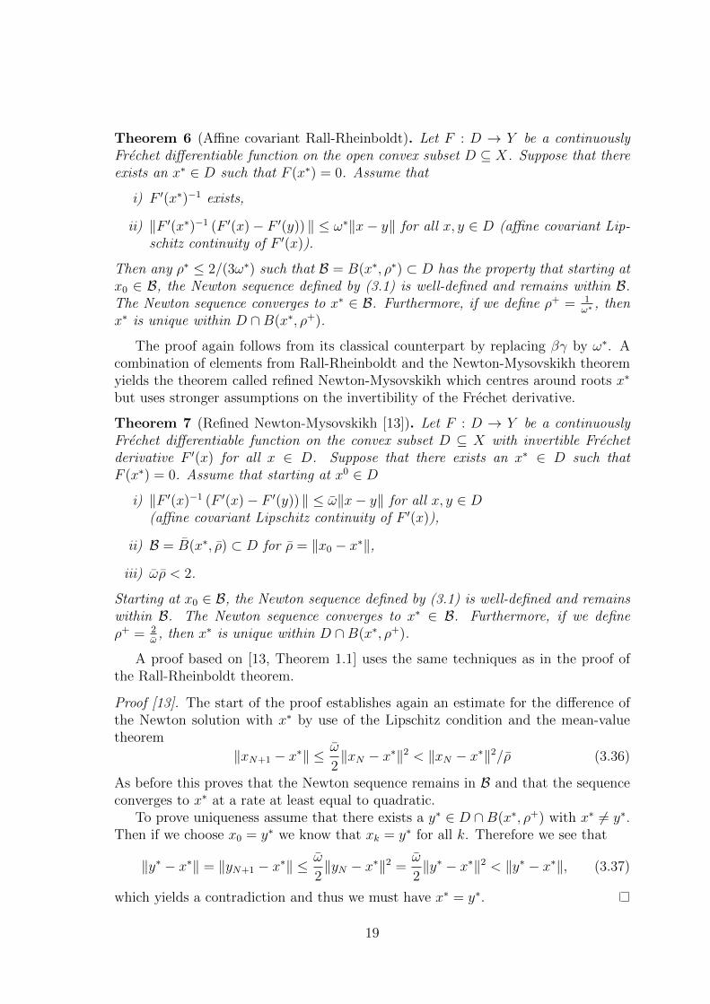
Theorem 6 (Affine covariant Rall-Rheinboldt). Let F : D → Y be a continuouslyFrechet differentiable function on the open convex subset D ⊆ X. Suppose that thereexists an x∗ ∈ D such that F (x∗) = 0. Assume that

i) F ′(x∗)−1 exists,

ii) ‖F ′(x∗)−1 (F ′(x)− F ′(y)) ‖ ≤ ω∗‖x− y‖ for all x, y ∈ D (affine covariant Lip-schitz continuity of F ′(x)).

Then any ρ∗ ≤ 2/(3ω∗) such that B = B(x∗, ρ∗) ⊂ D has the property that starting atx0 ∈ B, the Newton sequence defined by (3.1) is well-defined and remains within B.The Newton sequence converges to x∗ ∈ B. Furthermore, if we define ρ+ = 1

ω∗, then

x∗ is unique within D ∩B(x∗, ρ+).

The proof again follows from its classical counterpart by replacing βγ by ω∗. Acombination of elements from Rall-Rheinboldt and the Newton-Mysovskikh theoremyields the theorem called refined Newton-Mysovskikh which centres around roots x∗

but uses stronger assumptions on the invertibility of the Frechet derivative.

Theorem 7 (Refined Newton-Mysovskikh [13]). Let F : D → Y be a continuouslyFrechet differentiable function on the convex subset D ⊆ X with invertible Frechetderivative F ′(x) for all x ∈ D. Suppose that there exists an x∗ ∈ D such thatF (x∗) = 0. Assume that starting at x0 ∈ D

i) ‖F ′(x)−1 (F ′(x)− F ′(y)) ‖ ≤ ω‖x− y‖ for all x, y ∈ D(affine covariant Lipschitz continuity of F ′(x)),

ii) B = B(x∗, ρ) ⊂ D for ρ = ‖x0 − x∗‖,

iii) ωρ < 2.

Starting at x0 ∈ B, the Newton sequence defined by (3.1) is well-defined and remainswithin B. The Newton sequence converges to x∗ ∈ B. Furthermore, if we defineρ+ = 2

ω, then x∗ is unique within D ∩B(x∗, ρ+).

A proof based on [13, Theorem 1.1] uses the same techniques as in the proof ofthe Rall-Rheinboldt theorem.

Proof [13]. The start of the proof establishes again an estimate for the difference ofthe Newton solution with x∗ by use of the Lipschitz condition and the mean-valuetheorem

‖xN+1 − x∗‖ ≤ω

2‖xN − x∗‖2 < ‖xN − x∗‖2/ρ (3.36)

As before this proves that the Newton sequence remains in B and that the sequenceconverges to x∗ at a rate at least equal to quadratic.

To prove uniqueness assume that there exists a y∗ ∈ D ∩B(x∗, ρ+) with x∗ 6= y∗.Then if we choose x0 = y∗ we know that xk = y∗ for all k. Therefore we see that

‖y∗ − x∗‖ = ‖yN+1 − x∗‖ ≤ω

2‖yN − x∗‖2 =

ω

2‖y∗ − x∗‖2 < ‖y∗ − x∗‖, (3.37)

which yields a contradiction and thus we must have x∗ = y∗.

19

All the above theorems are stated in a general setting, with the only severe restric-tion being a local (affine covariant) Lipschitz continuity of the Frechet derivative ofthe function. Of course there are situations in which the function is in fact smootherthan demanded by the preceding theorems and this can lead to new convergencetheorems, which we will consider in the next section.

3.3 Convergence theorems for analytic functions

We step from continuously differentiable functions to the class of functions that areinfinitely differentiable, a concept known in finite dimensions as analyticity. In doingso we skip the classes of three, four, etc. times differentiable functions for which someliterature does exist, see for example [23]. The style and approach to those functionsin literature is, however, completely in line with the previous section and authorsmerely devise more complex majorant sequences.

Analytic functions are considered to be functions which can (at least locally) beexpanded in a convergent Taylor series, which is likely to be familiar for functions onR or C. To extend the ideas of analytic functions to general Banach spaces we firstneed to redefine a polynomial, which is a crucial concept in the definition of a powerseries.

Definition 3. A continuous m-homogeneous polynomial P is a function from X toY such that there exists a multi-linear map A of degree m with the property that forevery x ∈ X

P (x) = A(x, . . . , x) = A(xm) := Axm. (3.38)

A remark on notation, xm = (x, . . . , x) ∈ Xm is a m-tuple on which A acts. Normson multi-linear maps G : Xn → Y can be defined as induced norms by

‖G‖ = supx1 6=0,...xn 6=0

‖G(x1, . . . , xn)‖‖x1‖ . . . ‖xn‖

. (3.39)

Note that ‖P‖ ≤ ‖A‖ with equality if A is a symmetric multi-linear map. This nowallows us to define the concept of a power series.

Definition 4 ([33]). A power series from X to Y about x ∈ X is a series in x ∈ Xof the form

∞∑k=0

Pk(x− x), (3.40)

where Pk is a continuous k-homogeneous polynomial from X to Y .

A power series is said to be convergent around x if there exists some r > 0 suchthat for all x ∈ B(x, r) the power series converges uniformly in norm. Analyticfunctions are then defined by use of power series.

20

Definition 5. A function F : D → Y , with D ⊆ X an open subset is called analyticif for all x ∈ D there exists a r > 0 such that the function can be expanded in a

convergent power series, F (z) =∞∑k=0

1

k!F (k)(x)(z − x)k, for all z ∈ B(x, r) ⊂ D.

Here F (n)(x) is the n-th Frechet derivative at the point x and this is a symmetricmulti-linear map of degree n from Xn = X×· · ·×X to Y . The notation in Definition5 is thus equivalent to (F (n)(x))(z − x, . . . , z − x). The series expansion of F aroundx is called the Taylor series. One can now see that the power series in Definition 5is in fact a direct generalisation of the power series for functions of one variable. Infact, the Taylor series is the unique power series expansion of F at x just as is thecase for functions of one variable.

Before we proceed to the convergence theorems we need another auxiliary func-tional analysis result, the Cauchy-Hadamard theorem [33, Proposition 4.1], whichextends the idea of a radius of convergence for power series to a Banach space set-ting.

Theorem 8 (Cauchy-Hadamard [33]). Given a power series∑∞

k=0 Pk(x− x) from Xto Y about x ∈ X, The largest R such that the power series is uniformly convergenton every B(x, ρ) for 0 ≤ ρ < R is given by

1

R= lim sup

k→∞‖Pk‖1/k, (3.41)

and is called the radius of convergence of the power series.

Note that although F might be an entire function, i.e. analytic on X, this doesnot imply that its Taylor series around some x ∈ X converges on the whole of Xas this is only true for the finite dimensional case. See, for instance, [33, Remark7.1] for a counter example, signifying that there are in fact differences between thefinite dimensional case which we normally encounter and the formalism in (infinitedimensional) Banach spaces.

A related concept in complex analysis to analytic functions is that of a holomorphicfunction.

Definition 6. Let X and Y be complex Banach spaces. A function F : D → Y , withD ⊆ X an open subset, is called holomorphic if F is Frechet differentiable for allx ∈ D.

We thus see that all functions that we considered in the preceding section are infact holomorphic if X and Y are complex Banach spaces. Just as in finite dimensionalcomplex analysis the notion of holomorphic and analytic functions are equivalent ifwe have Banach spaces over C as pointed out by the following theorem.

Theorem 9 (Goursat [33]). Let X and Y be complex Banach spaces and F : D → Y ,with D ⊆ X an open subset, then the following statements are equivalent:

i) F is holomorphic,

21

ii) F is analytic.

Consequently, the results in this section will only consider a truly different classof functions F if we use real Banach spaces. In the case of complex Banach spacesthe assumptions in the previous section are actually more restrictive than we willsee in this section, because we previously considered Lipschitz continuous Frechetderivatives, whereas for the analytic functions in this section we just have continuousFrechet derivatives.

Now consider an F : X → Y analytic and the application of Newton’s method tofind its roots. A different class of convergence theorems can be derived in this case,based on initial work by Smale [45].

Smale convergence theorems

First we define an auxiliary quantity introduced by Smale

γ(x) = supk∈Nk≥2

∥∥∥∥F ′(x)−1F (k)(x)

k!

∥∥∥∥1/(k−1)

. (3.42)

This is a well-defined expression for analytic functions at points where the Frechetderivative is invertible. This follows from application of theorem 8 to the Taylor seriesof an analytic function F . Note furthermore that γ(x) is an affine covariant quantity.

We start with a convergence theorem similar in spirit to the Rall-Rheinboldttheorem which, instead of using an affine covariant Lipschitz condition on F ′, makesuse of evaluation of γ(x) at the root of F .

Theorem 10 (Smale’s γ-theorem [7]). Let F : D → Y with D ⊆ X an open subsetbe an analytic function. Suppose that there exists an x∗ ∈ D for which F (x∗) = 0 and

F ′(x∗)−1 exists. Let γ∗ = γ(x∗), then any ρ∗ ≤ 5−√

174γ∗

such that B = B(x∗, ρ∗) ⊆ D

has the property that starting at x0 ∈ B, the Newton sequence defined by (3.1) iswell-defined, remains within B. The Newton sequence converges to x∗ ∈ B, which isunique in B.

We note that this theorem does not seem to appear in literature as a result on itsown and is often merely used to proof another Smale theorem which we will presenthereafter. Nonetheless we state the theorem here as it is of interest for our purposes,because of the x∗-centred framework in which it is formulated. The theorem and proofare taken from [7, Theorem 8.1], but with some minor modifications to illustrate somesubtleties.

Proof [7]. Observation 1 (Invertibility of the Jacobian)Using the fact that F is analytic we expand its Frechet derivative in a Taylor series.

22

We find for some r > 0 and x ∈ B(x∗, r)

F ′(x∗)−1F ′(x) = F ′(x∗)−1

(F ′(x∗) +

∞∑m=1

F (m+1)(x∗)

m!(x− x∗)m

)(3.43)

= I +∞∑m=1

(1

m!F ′(x∗)−1F (m+1)(x∗)

)(x− x∗)m (3.44)

= I +G, (3.45)

which is now of the form I +G with G ∈ GL(Y ).Our objective is to prove that the Frechet derivative of F exists on B. In order

to do so we have to use that the Taylor series is defined on the whole of B, or simplysaid that the radius of convergence R of the Taylor series satisfies R ≥ ρ∗. This isa subtle point and has apparently been overlooked by many authors. The radius ofconvergence can be found by applying theorem 8 which yields

1

R= lim sup

n→∞n≥1

‖Pn‖1/n (3.46)

≤ lim supn→∞n≥1

∥∥∥∥ 1

n!F ′(x∗)−1F (n+1)(x∗)

∥∥∥∥1/n

(3.47)

≤ lim supn→∞n≥1

(n+ 1)1/n · lim supn→∞n≥1

∥∥∥∥ 1

(n+ 1)!F ′(x∗)−1F (n+1)(x∗)

∥∥∥∥1/n

(3.48)

= 1 · lim supm→∞m≥2

∥∥∥∥ 1

m!F ′(x∗)−1F (m)(x∗)

∥∥∥∥1/(m−1)

≤ γ∗. (3.49)

From this we can conclude that the radius of convergence satisfies R ≥ 1/γ∗ > ρ∗

and thus indeed we can use the Taylor series on B.Let u = ‖x−x∗‖γ∗. Under the assumption that u < 1−

√2/2, which is guaranteed

by x ∈ B, we find that using the power series

‖G‖ =

∥∥∥∥∥∞∑m=1

Pm(x− x∗)

∥∥∥∥∥ (3.50)

≤∞∑m=1

‖Pm(x− x∗)‖ (3.51)

≤∞∑m=1

‖Pm‖ ‖x− x∗‖m . (3.52)

23

Next we use the explicit form of the terms in the series expansion of G to find

‖G‖ ≤∞∑m=1

∥∥∥∥ 1

m!F ′(x∗)−1F (m+1)(x∗)

∥∥∥∥ ‖x− x∗‖m (3.53)

≤∞∑n=2

n

∥∥∥∥ 1

n!F ′(x∗)−1F (n)(x∗)

∥∥∥∥ ‖x− x∗‖n−1 (3.54)

≤∞∑n=2

n (γ∗ ‖x− x∗‖)n−1 (3.55)

=∞∑n=2

nun−1 ≤ 1

(1− u)2− 1 < 1. (3.56)

By using lemma 2 we then find that

‖F ′(x)−1F ′(x∗)‖ ≤ 1

1− ‖G‖≤ 1

1−(

1(1−u)2

− 1) =

(1− u)2

ψ(u), (3.57)

where ψ(u) = 1− 4u+ 2u2.Observation 2 (Evolution of Newton iterates)

We will use an induction argument to show that the Newton sequence remainsbounded within B and forms a converging sequence.

Suppose that we have a Newton sequence {xk} for k = 1, . . . , N such that xk ∈ B.If we use the Taylor series for F (xN) and F ′(xN) around x∗ we find that the nextiterate satisfies

‖xN+1 − x∗‖ =∥∥F ′(xN)−1F ′(x∗)

[−F ′(x∗)−1F (xN) + F ′(x∗)−1F ′(xN)(xN − x∗)

]∥∥(3.58)

=

∥∥∥∥∥F ′(xN)−1F ′(x∗)

[∞∑m=1

(m− 1)F ′(x∗)−1F (m)(x∗)

m!(xN − x∗)m

]∥∥∥∥∥(3.59)

Using the triangle inequality and the γ∗-condition we can derive

‖xN+1 − x∗‖ ≤(1− u)2

ψ(u)

∞∑m=1

∥∥∥∥(m− 1)F ′(x∗)−1F (m)(x∗)

m!(xN − x∗)m

∥∥∥∥ (3.60)

≤ (1− u)2

ψ(u)

∞∑m=1

(m− 1)

∥∥∥∥F ′(x∗)−1F (m)(x∗)

m!

∥∥∥∥ ‖xN − x∗‖m (3.61)

≤ (1− u)2

ψ(u)

∞∑m=1

(m− 1)(γ∗)m−1 ‖xN − x∗‖m (3.62)

= ‖xN − x∗‖(1− u)2

ψ(u)

∞∑m=1

(m− 1)um−1 (3.63)

= ‖xN − x∗‖(1− u)2

ψ(u)

u

(1− u)2= ‖xN − x∗‖

u

ψ(u). (3.64)

24

As xN ∈ B we find u < (5−√

17)/4 which implies u/ψ(u) < 1. Therefore we concludethat ‖xN+1 − x∗‖ < ‖xN − x∗‖. This proves that the sequence remains in B as thebase case k = 0 is satisfied trivially.

Using induction we can now show that ‖xN−x∗‖ < (u/ψ(u))N‖x0−x∗‖ and thus,we observe that xk → x∗.

The uniqueness proof follows that of the refined Newton-Mysovskikh theorem.

With this result Smale then derived his point estimate theorem which establisheslocal convergence of a point purely based on function evaluations at the starting pointand is more similar to Newton-Kantorovich and Newton-Mysovskikh in spirit.

Theorem 11 (Smale’s α-theorem [45]). Let F : D → Y with D ⊆ X an open subsetbe an analytic function. Assume that, starting at x0 ∈ X,

i) F ′(x0)−1 exists and let β0 = ‖F ′(x0)−1F (x0)‖,

ii) α(x0) = β0γ(x0) < α0, where α0 is a universal constant (α0 ≈ 0.1307),

iii) x0 ∈ B = B(x0, ρ0) ⊆ D, where ρ0 = 1−√

2/2γ(x0)

.

Then the Newton sequence started at x0 converges to a unique x∗ ∈ B(x0, 2β0) forwhich F (x∗) = 0 holds.

The universal constant α0 appears to be subject to debate as the optimal valuehas not been established as of yet and the best version we found in the literature isα0 = 3− 2

√2 [37].

25

3.4 Summary of local convergence theorems

In this chapter we have reviewed a collection of local convergence theorems for theclassical Newton’s method. Following an important observation by Deuflhard [12]we state all the final versions of the theorems in an affine covariant form. The the-orems share many general characteristics and mainly differ on just two points. Aclassification based on these differences is given in Table 3.1.

The first one is the reference frame of the theorem. With that we mean whetherthe theorems are centred around an initial guess x0 or around a root x∗. This willprove to be important in considering the deflation technique in the next chapter, wherewe will show that to incorporate deflation there is a clear preference for root-centredtheorems.

The other main difference between theorems is their restriction on the smooth-ness of the function. Here we make a distinction between real and complex Banachspaces. In the case of real Banach spaces, the minimal requirement seems to be aLipschitz continuous Frechet derivative on some open set D ⊆ X, which is equivalentto a bounded second Frechet derivative if a function is in fact twice differentiable. Byrequiring more smoothness in the form of analytic functions we can use a differentapproach and use Smale’s point estimation theories. In the case of a complex Ba-nach space the requirements for the theorems coincide, all theorems now require thefunction to be holomorphic. The Lipschitz continuity of the Frechet derivative is nowactually a more severe constraint than analyticity, which merely implies a continuousFrechet derivative.

Lipschitz continuous Frechet derivative Analytic function

x0

Newton-Kantorovich theorem 4Smale’s α-theorem 11

*Newton-Mysovskikh theorem 5

x∗Rall-Rheinboldt theorem 6

Smale’s γ-theorem 10*Refined Newton-Mysovskikh theorem 7

Table 3.1: Summary of local convergence theorems for Newton’s method. All theo-rems are understood to be in affine covariant form. The theorems are ordered by theircenter of convergence balls and requirements on the objective functions smoothness.*-Theorems assume invertibility of the Frechet derivative throughout the domain,whereas the others just assume invertibility at their respective centres of the conver-gence balls.

26

4. Local convergence of Newton’smethod and deflation

The local convergence theorems in the preceding chapter have been concerned withthe problem of finding a single solution to F (x) = 0. For our purposes, however wewant to be able to find multiple solutions. In this chapter we will therefore startderiving sufficient conditions that can guarantee the converge of Newton’s methodcombined with deflation to multiple solutions starting from a single initial guess x0.

4.1 Examples of local convergence to multiple so-

lutions

The theorems in chapter 3 can be used to prove quadratic convergence of an initialguess x0 to a root. We will first show by simple examples that it is possible toprove local quadratic convergence of a single initial point to multiple roots. Theseexamples also serve as an illustration for the differences in the convergence theoremsfor Newton’s method.

Example 1 (Quadratic polynomials). Let X = Y = C and f(x) = (x − 1)(x + 1).Note that due to the affine-covariant and affine-contravariant properties of Newton’smethod any quadratic polynomial with distinct roots can be brought into this form,so that the analysis of quadratic polynomials can be done purely on this specificexample.

It is sufficient to prove convergence to one of the roots of the quadratic polynomialsince after Wilkinson deflation the polynomial is linear which will result in Newton’smethod converging in one step. As the function is invariant under the transformationx 7→ −x we only consider the case <(x0) > 0.

Under the assumption x0 6= 0, the affine covariant Lipschitz constant for Newton-Kantorovich is given by ω0 = 1/|x0| and the initial Newton step by α = |x2

0−1|/2|x0|.To apply theorem 4 we need |1−1/x2

0| ≤ 1. As a result we find quadratic convergencetowards x = 1 for UNK = {x ∈ C : |1− 1/x2| ≤ 1}.

The affine covariant Lipschitz constant in the Rall-Rheinboldt (Theorem 6) isgiven by ω∗ = 1 and thus for all x ∈ URR = {x ∈ C : |1 − x| < 2/3} we findconvergence towards x = 1.

Note that for the refined Newton-Mysovskikh theorem we can choose the domainD for which we assume that f ′(x)−1 exists, and we take it to be equal to B(1, |x0−1|).Looking at the affine covariant Lipschitz constant we find ω = 1/(1 − |x0 − 1|) andwe find the exact same convergence region as for the Rall-Rheinboldt theorem.

In this simple case we can calculate Smale’s γ explicitly, which gives γ(±1) = 1/2and therefore ρ∗ = (5 −

√17)/2 ≈ 0.438. Convergence to x = 1 is thus guaranteed

for USγ = {x ∈ C : |1− x| < (5−√

17)/2} ⊂ URR.

27

Evaluation of Smale’s α(x0) can be done explicitly as well and yields α(x0) =|1−1/x2

0|/4. Convergence to x = 1 is thus guaranteed for USα = {x ∈ C : |1−1/x2| ≤4α0} ⊂ UNK.

The resulting convergence regions are sketched in Figure 4.1. A clear distinction inthe shape of the local convergence regions for the theorems which center convergenceballs around x0 versus those centred around x∗ can be seen.

−4 −3 −2 −1 0 1 2 3 4−4

−3

−2

−1

0

1

2

3

4

<(x)

=(x

)Newton-KantorovichRall-RheinboldtSmale-γSmale-α

Figure 4.1: Local convergence regions given by theorems in chapter 3 for the quadraticpolynomial f(x) = (x− 1)(x+ 1). The roots are indicated by •.

Example 2 (Cubic polynomials). Just as for the quadratic polynomials we use theinvariant properties of Newton’s method to construct a normal form for the cubicpolynomials with distinct roots, which can be chosen to be f(x) = (x+1)(x−a)(x−1)with a ∈ A = {x ∈ C : |x± 1| ≤ 2, x 6= ±1}. This can be achieved by using an affinetransformation which maps the roots with the greatest separation to ±1 respectively,the remaining root is closer to the roots and thus has to lie in A. The form is chosenso that deflation of this standard cubic we can arrive at the standard quadratic fromthe previous example. We construct a subset E ⊂ A such that if a ∈ E there exists apoint which converges quadratically to all the roots of the cubic polynomial.

Note that f ′(x) = 3x2 − 2ax − 1 so that f ′(a) = a2 − 1 6= 0. Given a convex setD ⊂ C we thus have

|f ′(a)−1 (f ′(x)− f ′(y)) | = 1

|1− a2||f ′(x)− f ′(y)| ≤ maxz∈D |f ′′(z)|

|1− a2||x− y|, (4.1)

using the mean value theorem 3. Now suppose the convex set D is an open ballB(a, q) ⊂ C. This allows us to find an affine covariant Lipschitz constant on D(possibly not the best one) as used in the theorem 6,

ω∗ =maxz∈D |6z − 2a|

|1− a2|=

4|a|+ 6q

|1− a2|,

28

where we have used that the affine transformation z 7→ 6z − 2a takes B(a, q) toB(4a, 6q). The element of this new ball furthest away from the origin then hasmodulus 4|a|+ 6q.

In order to use theorem 6 we need to have B (a, ρ∗) ⊂ D for ρ∗ ≤ 2/(3ω∗). Take

q = ρ∗ and then solving this inequality yields q ≤(√|a|2 + |1− a2| − |a|

)/3.

W.l.o.g. assume that <(a) ≥ 0 and let q =(√|a|2 + |1− a2| − |a|

)/3, so that

2/(3ω∗) = q. To gain quadratic convergence to all three roots it now suffices toshow that B (a, 2/(3ω∗)) ∩ B(1, 2/3) 6= ∅. The condition of intersecting balls from ageometrical point of view yields the condition q + 2/3 > |1 − a|. This now defines

the set E+ = {x ∈ A :(√|x|2 + |1− x2| − |x|

)+ 2− 3|1− x| > 0}. Consequently, if

a ∈ E the point 2a/3 + 1/3 is guaranteed to converge quadratically to firstly x = a,then x = 1 and finally to x = −1. Completely analogous we can define E− aroundx = −1 and their union creates the set E , depicted in Figure 4.2.

−1.5 −1 −0.5 0 0.5 1 1.5

−1.5

−1

−0.5

0

0.5

1

1.5

A

E

<(x)

=(x

)

Figure 4.2: Area within dotted lines depicts A and the shaded area shows E ⊂ A.If the root a of f(x) = (x + 1)(x − a)(x − 1) lies within E , there exists a pointwhich converges quadratically to all three roots of the cubic polynomial. The rootsat x = ±1 are indicated by •.

As we saw from the previous examples there are indeed functions for which thesituation sketch made in Figure 2.1 holds. The convergence balls using for examplethe Rall-Rheinboldt theorem grow after deflation which makes it possible for pointsto be contained in a convergence ball of a different root at every step of the deflation.This raises the question whether we can formalise sufficiency conditions for this tohappen in the case of deflation on general functions.

29

4.2 Convergence criteria for deflated functions

Having defined a general framework for deflation in Banach spaces we will now look atthe applicability of theorems in Chapter 3 in the case of deflation in its most generalform.

First we note that we can rule out the use of any theorem which is centred aroundthe initial guess x0 if we want to prove statements of convergence to multiple roots.This can be understood as follows. Suppose there exist x1 and x2 such that F (x1) =F (x2) = 0 and x1 6= x2. Now assume we consider an initial guess x0 that provablyconverges to x1 using a convergence theorem in the x0 framework. The result is a ρsuch that x1 ∈ B(x0, ρ) and x2 /∈ B(x0, ρ), see Figure 4.3a. Now after deflating Fwe have to consider M(x;x1)F (x). This deflated function in most cases will behavebadly at the deflated root. In the case of shifted norm-deflation (2.9) for examplethere will be a pole or discontinuity in the Frechet derivative at x = x1. In orderto prove convergence to x2 for the deflated function we would need to be able tofind a ρ′ > ρ such that x2 ∈ B(x0, ρ

′), but this would imply that x1 ∈ B(x0, ρ′), see

Figure 4.3b. Since the convergence theorems require the function to be well-behavedon these convergence balls and prove that the Frechet derivative is invertible, the illbehaviour at x1 poses a problem. As a result we will focus in the next section on thetheorems of the x∗-framework.

x∗1

x∗2

x0

D

ρ

(a) Convergence before deflation

x∗1

x∗2

x0

D

ρ′

(b) Convergence after deflation

Figure 4.3: Illustration of local convergence of the failure of convergence towardsmultiple roots in the x0-framework of the convergence theorems. In order to showconvergence to multiple solutions we need the convergence region to grow, i.e. ρ′ > ρ.This would however imply that the deflated root lies within the new convergenceregion, which poses regularity problems on the Frechet derivative of the deflatedfunction in the convergence region.

4.2.1 Deflation on analytic functions

In the case of an analytic function and under regularity conditions on the deflationoperator we can show that the deflated operator will remain well-behaved close tothe unknown roots.

30

Theorem 12. Let F : X → Y be an analytic function on an open subset D ⊆ X.Suppose that z ∈ D such that F (z) = 0 and the Frechet derivative F ′(z) is invertible.Furthermore assume that we have an x∗ ∈ X, x∗ 6= z, such that F (x∗) = 0. Givena deflation operator M(·;x∗) : D \ {x∗} → GL(Y, Z) which is analytic on an opensubset E ⊆ D \ {x∗} such that z ∈ E, then the following holds;

i) the Frechet derivative of the deflated operator M(x;x∗)F (x) is invertible at z,

ii) the deflated operator is analytic on the open subset E containing z.

Note that a shifted deflation operator, as defined by 2.9, satisfies these require-ments if the norm on X is (locally) analytic and we are close enough to the root x∗

in the sense that 0 < ‖x − x∗‖p < 2, because we want 1/‖x − x∗‖p to be analytic.In that case we can use the composition rule for analytic functions to show that thedeflation operator, which is now a composition of analytic operators, is indeed ana-lytic on some open set E ⊆ D \ {x∗}. The question whether a norm is analytic, orwhether a Banach space has an equivalent real analytic norm appears to be subjectof continuing study in functional analysis and we will not dive into detail here, butjust mention that analytic norms do in fact exist [24] and that for separable Hilbertspaces and Lp[0, 1] spaces with p an even integer we can approximate any equivalentnorm by real analytic norms [14].

In order to prove Theorem 12 we need a lemma generalising the Cauchy productformula for the product of two series in C to Banach space, which will allow us totake products and sums of power series.

Lemma 6 (Cauchy product formula [25]). Let X, Y, Z be Banach spaces and α :X×Y → Z a continuous bilinear map. Suppose that the series

∑∞n=0 xn and

∑∞n=0 yn

are absolutely convergent in X and Y and denote their sum by x ∈ X and y ∈ Yrespectively. Then

α(x, y) =∞∑n=0

n∑k=0

α(xk, yn−k). (4.2)

Proof of Theorem 12. By the product rule for differentiation we have

[M(x;x∗)F (x)]′ =M(x;x∗)F ′(x) +M′(x;x∗)F (x). (4.3)

Since z ∈ X is a root of the original functional F , the Frechet derivative of thedeflated functional at z becomesM(z;x∗)F ′(z). For any x ∈ D the deflation operatorM(x;x∗) ∈ GL(Y, Z) and thus it is invertible. The deflated functional evaluated z isthus invertible and (

[M(x;x∗)F (x)]′)−1∣∣∣z

= F ′(z)−1M(z;x∗)−1. (4.4)

As both F andM(·;x∗) are analytic on an open set around z we can expand them

31

in convergent Taylor series around z,

M(x;x∗) =∞∑k=0

1

k!M(k)(z;x∗)(x− z)k =

∞∑k=0

Qk(x− z), (4.5)

F (x) =∞∑k=0

1

k!F (k)(z)(x− z)k =

∞∑k=0

Pk(x− z), (4.6)

where Qk(x), Pk(x) are continuous k-homogeneous polynomials. Now we can applythe Cauchy product formula to the bilinear form α(x, y) = xy to find a power seriesexpansion of the deflated operator

M(x;x∗)F (x) =∞∑n=0

n∑k=0

Qk(x− z)Pn−k(x− z) =∞∑n=0

Rn(x− z), (4.7)

where Rn(x) is a n-homogeneous polynomial.The above argument can be repeated for any u ∈ E as both F and M(·;x∗)

are analytic and can be expanded in power series. There exists therefore an openneighbourhood U around all x ∈ E such that the deflated operator can be expandedinto a convergent power series. As the power series expansion of an operator isuniquely defined it follows from theorem 9 that the deflated operator is analytic onE.

A direct consequence of the above theorem is that Smale’s γ remains well-definedafter deflation.

Corollary 2. Under the assumptions in theorem 12, Smale’s gamma-function, givenby (3.42), is well-defined at z ∈ X for both the original function F (x) and the deflatedfunction M(x;x∗)F (x). In this case denote γ(x) as Smale’s gamma-function appliedto the deflated function M(x;x∗)F (x).

Although it is not clear from the above results what the relation is between γ(z)after deflation and γ(z) before deflation, we can conclude that after deflation withsuitable smooth operators that in principle at every stage of deflation there exist openneighbourhoods around the undiscovered roots for which quadratic convergence withNewton is guaranteed.

Note, though, that deflating a function can in fact result in γ(z) < γ(z) whichresults in larger convergence balls after deflation compared with the situation beforedeflation, as the following example shows.

Example 3 (Shrinking Smale’s gamma after deflation). We consider again the stan-dard cubic polynomial f(x) = (x+ 1)(x− a)(x− 1) with a ∈ A = {x ∈ C : |x± 1| ≤2, x 6= ±1} where x ∈ C. Explicitly calculating the Smale gamma-functions yields

γ(1) = max

{|3− a|2|1− a|

,1√

2|1− a|

}≥ 1

2,

γ(−1) = max

{|3 + a|2|1 + a|

,1√

2|1 + a|

}≥ 1

2,

32

where the inequality is derived from a ∈ A, which implies |1− a| ≤ 2 and |1 + a| ≤ 2,and the second term over which we take the maximum. Equality for both inequalitiesat the same time could only happen then if 2 = |1− a| = |1 + a|, i.e. a = ±i

√3, but

in that case γ(±1) =√

3/2 > 1/2. So at least one of the inequalities is strict.After deflation of the root a we can use Example 1 to find that γ(±1) = 1/2.

Therefore we see that at least one of the gamma functions shrinks after deflation.

Combining Theorem 12 with the idea of overlapping convergence balls as in Figure2.1 we get the first sufficient conditions for convergence to multiple roots from a singleinitial guess using deflation and Newton’s method.

Theorem 13 (Deflated Smale’s γ-theorem). Let F : X → Y be an analytic functionon an open subset D ⊆ X. Suppose that z1, z2 ∈ D such that F (z1) = F (z2) = 0 andthe Frechet derivatives F ′(z1) and F ′(z2) are invertible. Given a deflation operatorM(·; z1) : D \ {z1} → GL(Y, Z) which is analytic on an open subset E ⊂ D \ {z1}such that z2 ∈ E, then define

i) γ(x) as Smale’s gamma-function defined by (3.42) applied to M(x; z1)F (x),

ii) γ∗1 = γ(z1) and ρ∗1 = 5−√

174γ∗1

,

iii) γ∗2 = γ(z2) and ρ∗2 = 5−√

174γ∗2

.

If ‖z1 − z2‖ < ρ1 + ρ2 for some ρ1 ≤ ρ∗1 and ρ2 ≤ ρ∗2 such that B1 = B(z1, ρ1) ⊂ Dand B2 = B(z2, ρ2) ⊂ E, then there exists an x0 ∈ B1∩B2. Starting from this x0 withNewton’s method we first converge to z1 ∈ D and then after deflation using M(·; z1)we converge to z2 ∈ E.

Note that by Theorem 12 all definitions in Theorem 13 are well-defined. A proofapplies Theorem 12, Theorem 10 and an overlapping condition on convergence ballsbefore and after deflation as depicted in Figure 2.1.

As the above results are restricted to the case of analytic functions one could aska similar type of question for general functions, as treated in Section 3.2.

4.2.2 Deflation on general functions

We now consider functions which are not necessarily analytic, but for which we canprove local convergence of Newton’s method. As a crucial ingredient of the affinecovariant theorems in Section 3.2 is the affine covariant Lipschitz continuity of theFrechet derivative F ′, we first state a lemma on the product of Lipschitz continuousfunctions.

Lemma 7 (Product of Lipschitz continuous functions). Let X, Y, Z be Banach spacesand G : X → L(Y, Z) and F : X → Y be Lipschitz continuous functions on the opensubset D ⊆ X with Lipschitz constants ωF and ωG respectively. Assume furthermorethat F is bounded on D, i.e. there exist NF , NG ∈ R such that for all x ∈ D we have‖F (x)‖ < NF and ‖G(x)‖ < NG, as G is bounded by definition. Then the productGF : X → Z is bounded and Lipschitz continuous on D with Lipschitz constant(NFωG +NGωF ).

33

For a proof see Appendix A.2. Note that the given Lipschitz constant might notbe the best Lipschitz constant.

This now sets conditions for our deflation operator such that we can apply theRall-Rheinboldt convergence theorem to deflated functions.

Theorem 14. Let F : D → Y be a continuously Frechet differentiable function onthe open convex subset D ⊆ X. Suppose that z ∈ D such that F (z) = 0 and theFrechet derivative F ′(z) is invertible. Furthermore assume that we have an x∗ ∈D, x∗ 6= z, such that F (x∗) = 0. Suppose then that we have a deflation operatorM(·;x∗) : D \ {x∗} → GL(Y, Z) and an open bounded convex subset E ⊆ D \ {x∗}with z ∈ E such that the following conditions hold:

i) F satisfies the two Rall-Rheinboldt conditions around z ∈ D (see theorem 6),

ii) M(x;x∗) is continuously Frechet differentiable for all x ∈ E,

iii) ‖M′(x;x∗)−M′(y;x∗)‖ ≤ ωM′‖x− y‖ for all x, y ∈ E.

Then there exists a ρ > 0 such that if we start at x0 ∈ B = B(z, ρ) the Newton se-quence defined by (3.1) on the deflated functionM(x;x∗)F (x) is well-defined, remainsin B and converges to z ∈ B.

Note that a shifted deflation operator, as defined by 2.9, satisfies these require-ments under the condition that the norm on X is (locally) at least twice continuouslydifferentiable on E (this implies a Lipschitz continuous Frechet derivative as E isbounded). In that case we can use the composition rule for differentiable functions toshow that the deflation operator, which is now a composition of differentiable opera-tors, is indeed twice continuously differentiable E. The Lp spaces for 1 < p <∞ andSobolev spaces (W k,p for k ∈ N and 1 < p < ∞) are reflexive spaces and thereforeadmit a continuously differentiable norm on any open subset not containing zero,see for example [20]. The question whether a continuously twice differentiable normexists seems to be a more involved question in functional analysis. We point out thatfor 2 ≤ p <∞ the Lp standard norm is at least twice continuously differentiable [46,Theorem 8] and that Banach spaces that are isomorphic to a Hilbert space can beequipped with twice differentiable norms as well [29, 17].

This statement in essence states conditions for which the Rall-Rheinboldt theoremis not only applicable to the original function, but to the deflated function as well.

Proof. To start with we know by the same reasoning as in theorem 12 that the Frechetderivative of M(x;x∗)F (x) is invertible at z.

As F (x) andM(x;x∗) are continuously Frechet differentiable on E we know thatthey are Lipschitz continuous as well. Being Lipschitz continuous also implies thatthe operators are bounded on E and thus F (x), F ′(x),M(x;x∗) and M′(x;x∗) areall bounded on E.

As a result we know that the Frechet derivative of the deflated operator

(M(x;x∗)F (x))′ =M(x;x∗)F ′(x) +M′(x;x∗)F (x) (4.8)

34

is Lipschitz continuous by use of the triangle inequality and Lemma 7. Thereforethere exists some (affine covariant) ω > 0 such that∥∥∥([M(z;x∗)F (z)]′

)−1[(M(x;x∗)F (x))′ − (M(y;x∗)F (y))′]

∥∥∥ ≤ ω‖x− y‖, (4.9)

for all x, y ∈ E. This means that the affine covariant Rall-Rheinboldt theorem canbe applied to both F (x) and M(x;x∗)F (x), proving the claim in the theorem.

Now we can state sufficient conditions for a general function to convergence totwo solutions by using deflation and Newton’s method. The proof simply applies theprevious theorem and the Rall-Rheinboldt theorem 6.

Theorem 15 (Deflated Rall-Rheinboldt). Let F : D → Y be a continuously Frechetdifferentiable function on an open subset D ⊆ X. Suppose that z1, z2 ∈ D such thatF (z1) = F (z2) = 0. Let E1 be an open convex subset E1 such that E1 ⊂ D \ {z2}and z1 ∈ E1. Furthermore let E2 be an open bounded convex subset E2 such thatE2 ⊂ D \ {z1} and z2 ∈ E2. Additionally let M(·; z1) : D \ {z1} → GL(Y, Z) be adeflation operator such that the following conditions hold

i) F ′(z1)−1 and F ′(z2)−1 exist,

ii) ‖F ′(z1)−1 (F ′(x)− F ′(y)) ‖ ≤ ω∗1‖x− y‖ for all x, y ∈ E1,

iii) ‖F ′(z2)−1 (F ′(x)− F ′(y)) ‖ ≤ ω∗2‖x− y‖ for all x, y ∈ E2,

iv) M(x; z1) is continuously Frechet differentiable for all x ∈ E2,

v) ‖M′(x; z1)−M′(y; z1)‖ ≤ ωM′‖x− y‖ for all x, y ∈ E2.

Then there exists a ω2 > 0 such that for all x, y ∈ E2 there holds∥∥∥([M(z2; z1)F (z2)]′)−1

[(M(x; z1)F (x))′ − (M(y; z1)F (y))′]∥∥∥ ≤ ω2‖x− y‖. (4.10)

If ‖z1 − z2‖ < ρ1 + ρ2 for some ρ1 ≤ 2/(3ω∗1) and ρ2 ≤ 2/(3ω2) such that we haveB1 = B(z1, ρ1) ⊂ E1 and B2 = B(z2, ρ2) ⊂ E2, then there exists an x0 ∈ B1 ∩ B2.Starting from this x0 with Newton’s method we first converge to z1 ∈ E1 and thenafter deflation using M(·; z1) we converge to z2 ∈ E2.

Note that a crude upper bound for ω2 could be derived using Lemma 7, thetriangle inequality and bounds on the norms of F (x),M(x; z1) and their Frechetderivatives. The Lipschitz constant derived in this way is, however, likely to be agross overestimation of the optimal Lipschitz constant and therefore might not beuseful in practice.

We conclude with the observation that in order to derive sufficient conditions forconvergence we imposed the same regularity conditions on the deflation operator asthose imposed on the original function. This seems natural as we want their product,the deflated function, to satisfy similar regularity conditions in order to apply thelocal convergence theorems from Chapter 3.

35

5. Bifurcation diagrams and deflation

Now we turn our attention to an application of the method of deflation in findingmultiple solutions, namely the construction of bifurcation diagrams. We will firstgive a short introduction to the numerical computation of bifurcation diagrams usingso-called continuation techniques. Then we will highlight where deflation can com-plement the traditional numerical bifurcation toolbox. In practice we observe thatfor a range of illustrative problems with deflation and continuation combined we cantrace out bifurcation diagrams where continuation alone fails.

Part of the code used for this thesis is publicly available at https://bitbucket.org/CasperBeentjes/files-msc-dissertation.

5.1 Numerical bifurcation techniques

Branch continuation

We return to the original problem

F (u, λ) = 0, (5.1)

and suppose for the moment that we are initially given a root (u, λ). A naturalquestion now is whether we can solve 5.1 for u(λ), i.e. whether we can find a relationbetween the output of the model and the controls. Sufficient conditions for such acurve to exist are given by the implicit function theorem [26, Theorem 13.22]. Theymainly require an invertible partial Frechet derivative with respect to u, denoted Fu,at the given roots and result in an open neighbourhood around the given root forwhich u(λ) such that u(λ) = u is uniquely defined and a root to (5.1). As theseconditions are satisfied away from bifurcation points we can hope to trace out thesecurves by making small steps along the curve, an idea which was already known toPoincare [38], and is known under the name continuation.

In this classical setting of continuation the solution curve is parametrised by thenatural occurring parameter for the problem, namely λ. This parametrisation workswell in regions where Fu is non-singular so that we are guaranteed to have a uniqueparametrisation by the implicit function theorem. Note, however, that exactly atthe bifurcation points we see that Fu becomes singular and we lose uniqueness whichresults in a breakdown of our parametrisation. There are multiple ways to elude thisproblem and one of the most widespread options is to change the parametrisation ofthe solution branch such that at bifurcation points the partial Frechet derivative isnon-singular. A natural way to parametrise a curve is the arclength parametrisationwhich is depicted in Figure 5.1. If we denote the arclength parameter by s we nowlook for u(s) and λ(s) and have to add to (5.1) the arclength constraint to get a closed

36

system of equations. Doing so we arrive at

F (u(s), λ(s)) = 0, (5.2a)∥∥∥∥(du(s)

ds,dλ(s)

ds

)∥∥∥∥U×Λ

= 1. (5.2b)

With this added equation we are now able to continue branches through bifurcationpoints and we compute a bifurcation curve parametrised by s instead of λ.

λ0 λ1

u0

ucor

upred

∆s

predictor pathcorrector path

λ

u

Figure 5.1: Illustration of a predictor-corrector step for a scalar problem, where wehave used a tangent predictor to make an arclength step of length ∆s. The predictorstep is shown in blue and serves as an initialisation for the correction step, whosepath is shown by the dashed line.

We make use of a standard framework in numerical bifurcation analysis, predictor-corrector methods, which we sketch in Figure 5.1. One of the most used predictorsteps is based on the observation that along the curve, parametrised by λ, we have

0 = Fu(u, λ)uλ + Fλ(u, λ), (5.3)

known as the Davidenko equation. If given (u, λ) we can solve this for the tangentvector uλ. Note that in the natural parametrisation this equation breaks down atthe bifurcation due to the Jacobian Fu becoming singular. To overcome this problemwe again use the arclength parametrisation (5.2) and solve for a tangent vector,depending on s, in this augmented system, which is done by solving

Fudu(s)

ds+ Fλ

dλ(s)

ds= 0, (5.4a)∥∥∥∥(du(s)

ds,dλ(s)

ds

)∥∥∥∥U×Λ

= 1. (5.4b)

37

One constructs a predictor for a new solution in this tangent direction and uses thisas an initial guess for the computation of the corrected solution which should lie onour bifurcation curve again as depicted in Figure 5.1.

Therefore under the assumption of a starting point on the branch, or at least apoint sufficiently close for Newton to converge, we have a numerical procedure to traceout the solution branch. For a more detailed treatment of arclength continuation anddifferent continuation techniques see, for example, [44].

Branch detecting and branch switching

In addition to continuation techniques we need methods which can detect bifurcationpoints and a device that gives us the option to change solution branch at thesebifurcation points. The detection of a bifurcation is often done by looking at a testfunction, which is constructed such that it has a zero at bifurcation points. Thespecific form of the test function relies heavily on the type of bifurcation one wantsto detect. The type of bifurcation points is determined by the behaviour of theeigenvalues of the Jacobian Fu and in practice test functions therefore rely often oncalculation of either eigenvalues or determinants of the Jacobian, which is numericallyexpensive. This makes this approach not scalable to large-scale systems, such as thosearising in discretisations of PDEs, as the cost of the test-function becomes prohibitive.We will not discuss test functions in more detail here, but instead refer the reader to[28, 44].

Having detected a bifurcation point one now knows that multiple solutions haveto exist close to this point. Different techniques, dependent on the type of bifur-cation, have been devised to switch to different branches at bifurcation points andwe refer for details again to [28, 44]. Having switched branches we can, once more,use continuation techniques to trace out these branches fully. A sketch of how theaforementioned techniques are combined is given in Figure 5.2.

λ

J(u

)

(a) Detect bifurcation point

λ

J(u

)

(b) Switch to new branch

λ

J(u

)

(c) Continuation new branch

Figure 5.2: Illustration of standard numerical bifurcation algorithm. We start outby continuation of a branch as in Figure 5.2a. If we detect a bifurcation point wecan use specialised techniques to switch branch at the bifurcation point, depicted inFigure 5.2b. If we have a point on the new branch we can use standard continuationto trace out the new branch as in the rightmost figure.

38

5.2 Deflation and continuation combined

As mentioned in the introduction there is a flaw in the current numerical bifurcationalgorithms in the sense that they are not able to detect different branches in theabsence of a bifurcation point. A standard situation in which this might arise is inthe case of bifurcation branches which are disconnected from the initial branch suchas we saw in Figure 1.3. The numerical continuation techniques are capable of tracingout branches if and only if we can initialise them with a point which actually lies on thesolution branch. The problem of tracing out diagrams with disconnected branches,such as in Figure 5.3, now asks for a method to calculate multiple solution pointsfor a given parameter value. The deflation technique as discussed in the previouschapters can provide an answer to this problem and we will now shortly discuss twonovel applications of augmenting numerical bifurcation algorithms with deflation.

Detecting (disconnected) branches

As deflation is able to compute multiple solutions from one single initial guess, wepropose the augmentation of numerical bifurcation analysis with deflation in thefollowing way; we start with a given initial solution to trace out an initial branch.If the parameter λ reaches some pre-determined value λ we stop the continuationand we thus have some solution (u, λ) to (5.1). Instead of tracing a branch we nowlook for a solution to (5.1) at λ + ∆λ based on our knowledge of the solution atλ, i.e. we use u as an initial guess for the problem at parameter λ + ∆λ. If ∆λ issufficiently small, this will at least yield the continuation of the solution u on thesame branch. Having found this continuation we can then employ deflation, whichwill prevent the solver to converge to the same branch again. If we now retry with uas an initial guess we are guaranteed not to converge to the same branch again. Undersuitable conditions we can now find different solutions to (5.1) for the same parametervalue, which thus must lie on a different branch. In this way we can generate initialpoints on multiple branches and as we now have good initial points we can again usecontinuation techniques to fully trace out these branches. For a sketch of this methodsee Figure 5.3.

Note that this approach does not rely on either the presence or proximity of abifurcation point and can thus be applied to find disconnected branches.

Branch switching

The previous framework provides a method to find disconnected branches by usingdeflation at some specific parameter values, without any extra knowledge on thebifurcation structure of the problem. If we, however, do know more details about thespecific bifurcation structure in the form of the approximate location of a bifurcationpoint we can use this to our advantage. Close to a bifurcation point, the solutionswhich emanate from this point will be close to each other. This means that it islikely that an initial guess close to the bifurcation point will be able to yield multiplesolutions using deflation. Deflation can therefore be used to perform branch switching.

39

λ

J(u

)

(a) Initial continuation

λ

J(u

)

(b) Deflate to find multiplebranches

λ

J(u

)

(c) Continuation of branches

Figure 5.3: Illustration of the use of deflation in numerical bifurcation analysis. Westart out by continuation of a branch as in Figure 5.3a. Along our branch we stopand fix the parameter λ and attempt a deflation step to find multiple solutions forthis parameter value as in Figure 5.3b. If the deflation step is successful we have apoints on multiple branches and we can use standard continuation to trace out thesebranches as in the rightmost figure.

Although many different branch switching techniques do already exist, deflation isuseful in this context for two reasons.

First of all its generality, as branch switching with deflation is not dependenton the bifurcation type and can be used for a variety of bifurcations. The onlyrequirement that we need for deflation is that the problem can be formulated as asystem of equations of the form (5.1).

More importantly, branch switching with deflation can be made scalable. Theclassical branch switching techniques depend heavily on detection of the bifurcationpoint, which is computationally expensive. By contrast, if a good preconditioner isavailable for the underlying problem Farrell et al. [18] showed that the deflated systemscan be solved with the same computational efficiency as the underlying undeflatedsystem. Deflation for branch switching is thus the first scalable bifurcation technique.

5.3 Comparison with existing software

AUTO-07P

A large collection of software packages is available for numerical bifurcation analysisand an extensive list is described in [16]. One of the most widely used packages isAUTO-07P [15], which is written in Fortran 95 and partially equipped with a Pythonwrapper. The program is known for its reliability and offers both continuation andbranch switching algorithms for various types of bifurcations. AUTO-07P can applyits bifurcation analysis tools to two different classes of equations. First of all it cando a limited analysis on algebraic systems of the form

0 = F (u, λ), u ∈ Rn, λ ∈ Rm. (5.5)

40

This is for example useful in order to track bifurcations of steady state solutionsto a system of ODEs as this naturally results in a system of the form (5.5). Thesecond class of problems for which it can be used are one-dimensional boundary valueproblems (BVPs) of the form

u′(τ) = F (u(τ), λ), u(τ) ∈ Rn, λ ∈ Rm, τ ∈ [a, b], (5.6)

with boundary conditions and possibly integral constraints. Besides its use in lookingat bifurcation diagrams for BVPs this also allows one to investigate the stationarystates of certain parabolic PDEs describing reaction-diffusion equations of the form

uτ = Duxx + F (u, λ), u(x) ∈ Rn, λ ∈ Rm, x ∈ [a, b], (5.7)

where D is a diagonal Rn×n matrix containing the diffusion constants. The steadystates to this problem can be rewritten to (5.6).

Practical implementation deflation and continuation

We compare the bifurcation diagrams computed with AUTO-07P with our imple-mentation of deflation and continuation techniques. Our implementation was writ-ten in FEniCS [31], an automated programming environment for solving differentialequations using the finite element method (FEM), which we control using a Pythoninterface. We need to supply the equations in variational form, see [31], and the FEMdiscretisation to be used. FEniCS then assembles the discretised system of FEMequations which can be solved using numerical linear algebra software, in this casethe PETSc toolbox [4, 5, 10] in combination with the MUMPS package [1, 2].

To carry out the numerical bifurcation analysis we use an arclength continuationand deflation class written for FEniCS by P.E. Farrell [19] augmented by a branchswitching method purely based on deflation and a bifurcation detector based on thedeterminant test function. Our implementation of branch switching is thus purelybased on deflation in contrast to other software such as AUTO-07P. The algorithmgives the option to only switch branches at bifurcation points or to safeguard againstmissed branches by using deflation away from bifurcation points at points specifiedby the user.

5.3.1 Steady state continuation

We consider the problem of steady state continuation of ODEs, a BVP and a non-linear diffusion equation so that we can make use of AUTO-07P. We assume that weare initially given a steady state by either an explicit construction, a homotopy [44]or by integrating the time-dependent problem.

Algebraic problems

The first problem that we consider is the cusp, the second of the elementary catas-trophes in catastrophe theory, which can depend on two parameters λ and µ. TheODE that we consider is

u′ = u(λ− u2) + µ, (5.8)

41

where now u(t) and u′ means differentiation with respect to t. We are interested inthe steady states of this ODE as a function of the parameters, which can be achievedby setting u′ = 0 and solving the algebraic equation.

We start with the case µ = 0 and allow λ to vary. This is now the normal formof a pitchfork bifurcation in which two non-trivial (symmetrical) solutions emanatefrom a trivial branch in the bifurcation point. Since the bifurcation point connectsall branches, both AUTO-07P and our deflation implementation trace out the fullbifurcation diagram, see Figure 5.4a.

−2 −1.5 −1 −0.5 0 0.5 1 1.5 2−1.5

−1

−0.5

0

0.5

1

1.5

λ

u

DeflationAUTO-07P

(a) µ = 0

−2 −1.5 −1 −0.5 0 0.5 1 1.5 2−1.5

−1

−0.5

0

0.5

1

1.5

λ

u

DeflationAUTO-07P

(b) µ = 0.1

Figure 5.4: Bifurcation diagram for (5.8) as computed by AUTO-07P and the de-flation technique. For AUTO-07P we plot a data point every 2 steps. In the caseof µ = 0 there is a supercritical pitchfork bifurcation which connects all branches,whereas for µ = 0.1 we see that the symmetry of the pitchfork bifurcation has beenbroken and the branches are disconnected. In this case AUTO-07P can only find onebranch.

If we now set µ 6= 0 the reflection symmetry u 7→ −u gets broken and we arriveat the imperfect pitchfork bifurcation. This is an example of a bifurcation diagramwith disconnected branches. We have one trivial branch and two branches whicharise from a fold bifurcation and do not connect with the trivial branch. As a resultAUTO-07P is not able to compute the full bifurcation diagram if we start from thetrivial branch, see Figure 5.4b.

The next problem is inspired by Rosenblat and Davis [41] who studied bifurcationsat infinity as a possible explanation of observations in stability analysis of Hagen-Poiseuille flow and Couette flow. We start with the ODE

u′ = −λu+ u2 − u3, (5.9)

and again set u′ = 0. Now the bifurcation structure consists of a trivial branch andtwo solutions emanating from a subcritical fold bifurcation or saddle-node bifurcationat λ = 1/4. The non-trivial branches connect with the zero branch in a transcriticalbifurcation at λ = 0 and the bifurcation diagram is thus fully connected. Deflation

42

and AUTO-07P therefore correctly compute the full bifurcation diagram, see Figure5.5.

−2 −1.5 −1 −0.5 0 0.5 1−1

−0.5

0

0.5

1

1.5

2

λ

u

DeflationAUTO-07P

Figure 5.5: Bifurcation diagram for (5.9) as computed by AUTO-07P and the defla-tion technique. For AUTO-07P we plot a data point every 2 steps. There are twobifurcation points, a transcritical bifurcation at λ = 0 and a subcritical fold bifur-cation at λ = 1/4, which connect all the branches. Both AUTO-07P and deflationcompute the full bifurcation diagram.

If we now, however, make the transformation µ = 1/λ we drastically change thebifurcation diagram. We consider,

u′ = −uµ

+ u2 − u3, (5.10)

for µ > 0. We still have a trivial branch and two non-trivial branches originating ina supercritical fold bifurcation at µ = 4. However, we see now that the transcriticalbifurcation at λ = 0 becomes a bifurcation at µ = ∞ and as a result the branchesonly connect at infinity, which leaves them uncomputable to AUTO-07P, see Figure5.6.

The seemingly disconnected branches are important to the understanding of theproblem. A linear stability analysis would tell that the trivial branch is stable, butfor sufficiently large µ any positive perturbation would make the solution switch toone of the disconnected branches and this indicates that a linear stability analysiscan yield misleading results.

The previous examples show that deflation can trace out complete diagrams whereAUTO-07P fails in the case of algebraic problems. For the preceding examples thisresult could have been anticipated based on the results in Section 4.1 and the obser-vation that the considered problems were in fact all cubic polynomials. We will nowshow that in the case of more complicated problems deflation still gives better resultsthan AUTO-07P.

43

0 5 10 15 20 25 30 35 40

0

0.2

0.4

0.6

0.8

1

µ

u

DeflationAUTO-07P

Figure 5.6: Bifurcation diagram for (5.10) as computed by AUTO-07P and the de-flation technique. For AUTO-07P we plot a data point every 20 steps. There is onefinite bifurcation point, a supercritical fold bifurcation at µ = 4. The branches arehowever disconnected for all finite values of µ. One of the branches that emanatesfrom the fold bifurcation connects to the trivial branch at infinity. AUTO-07P doesnot detect a bifurcation point and thus only finds the trivial branch by continuation,whereas deflation traces out the full bifurcation diagram.

Boundary value problems

We now return to the problem sketched in the introduction of a slender beam undera loading, where we assume the loading to be in the longitudinal direction as inFigure 1.2. This problem has a long mathematical history tracing back to Galileo,the Bernoulli family and Euler [30]. It was the latter who showed that the deformationof the beam can be described in terms of the angle θ made relative to the verticalaxis as a function of the arclength s. If the beam is subject to a transversal force thesteady states of the beam are governed by Eulers elastica equation

θss + λ2 sin(θ) = µ, 0 ≤ s ≤ 1, (5.11a)

θ(0) = θ(1) = 0, (5.11b)

where λ is a non-dimensional load and µ depicts a non-dimensional transversal force.In the case µ = 0, i.e. in the absence of a transversal force, the initially straightsolution, θ ≡ 0, forms the trivial branch and is valid for all s. A series of pitchforkbifurcations at λ = mπ for m ∈ N result in the buckled modes emanating fromthe trivial branch. Both deflation and AUTO-07P therefore compute a completebifurcation diagram, see Figure 5.7a.

If we introduce a transversal force by taking µ 6= 0 we destroy a reflection sym-metry, just as we saw for the cusp bifurcation. The initial branch now disconnectsfrom all the other branches in a similar fashion as we observed before. The differencenow, however, is that there is an infinite number of branches which originally wereconnected to the initial branch and which now become disconnected. The result is

44

0 0.5 1 1.5 2 2.5 3 3.5 4−3

−2

−1

0

1

2

3

λ/π

σ‖u‖ L

2

DeflationAUTO-07P

(a) µ = 0

0 0.5 1 1.5 2 2.5 3 3.5 4−3

−2

−1

0

1

2

3

λ/π

σ‖u‖ L

2

DeflationAUTO-07P

(b) µ = 0.5

Figure 5.7: Bifurcation diagram for (5.11) as computed by AUTO-07P and the de-flation technique, where we take the scalar measure J(u) = σ‖u‖L2 , a signed norm.Here σ is given by σ = ux(0). For AUTO-07P we plot a data point every 8 steps. Inthe case of µ = 0 a series of supercritical pitchfork bifurcations at λ = mπ for m ∈ Nconnects all branches. For µ = 0.1 we see that the symmetry of the pitchfork bifur-cation has been broken and the branches are disconnected. In this case AUTO-07Pcan only find one branch.

that those branches are not found by continuation in AUTO-07P, yielding a very un-satisfactory representation of the bifurcation structure. Deflation on the other handis able to trace out disconnected branches as we see in Figure 5.7b.

Lastly we return to the work by Rosenblat and Davis [41] on bifurcations frominfinity. We consider the PDE

ut =uxxµ

+ u2 − u3, 0 ≤ x ≤ 1, µ > 0, (5.12a)

u(0, t) = u(1, t) = 0, (5.12b)

u(x, 0) = u0(x), (5.12c)

and look for its steady state solutions. As one can see, the trivial state is a solution forall µ. Analogous to (5.10) Rosenblat and Davis showed using singular perturbationtheory that there are two non-trivial solutions which emanate from a supercriticalfold bifurcation and one of these branches connects with the trivial branch at µ =∞.These two non-trivial branches can not be found by AUTO-07P using continuationand bifurcation tools, see Figure 5.8.

This PDE can be used to show that there exist systems in which an infinite numberof periodic solutions of small norm bifurcate from the trivial solution at infinity. Thishas implications for the use of standard analytic methods to compute bifurcationsolutions [41].

If we transform the system to a form similar to (5.9) by identifying λ = 1/µ,

ut = λuxx + u2 − u3, 0 ≤ x ≤ 1, (5.13)

45

0 20 40 60 80 100 120 140 160 180 200

0

0.2

0.4

0.6

0.8

1

µ

‖u‖ L

2

DeflationAUTO-07P

(a) Bifurcation diagram (5.12)

0 0.1 0.2 0.3 0.4 0.5 0.6 0.7 0.8 0.9 1

0

0.1

0.2

0.3

0.4

0.5

0.6

0.7

0.8

x

u

(b) Solutions (5.12) at µ ≈ 47.303

Figure 5.8: Bifurcation diagram for (5.12) as computed by AUTO-07P and the de-flation technique, where we take the scalar measure J(u) = ‖u‖L2 . Solutions at • aredepicted in Figure 5.8b.For AUTO-07P we plot a data point every 100 steps. There is one finite bifurcationpoint, a supercritical fold bifurcation at µ ≈ 41.157. One of the branches whichemanates from this fold bifurcation connects to the trivial branch at infinity. AUTO-07P does not detect a bifurcation point and thus only finds the trivial branch bycontinuation, whereas deflation traces out the full bifurcation diagram.

with the same boundary and initial conditions, one would expect to move the bifur-cation at infinity to λ = 0. However, we do not detect a bifurcation point on thetrivial branch using AUTO-07P, see Figure 5.9. A possible explanation would be thatthe point λ = 0 is at the same time a singular point for the equation and AUTO-07Pmight not be suited to solve such problems. Deflation with the bifurcation detectoris able to trace out the full diagram as shown in Figure 5.9.

46

−0.3 −0.25 −0.2 −0.15 −0.1 −0.05 0 0.05−1

−0.75

−0.5

−0.25

0

0.25

0.5

0.75

1

λ

σ‖u‖ L

2

DeflationAUTO-07P

(a) Bifurcation diagram (5.13)

0 0.1 0.2 0.3 0.4 0.5 0.6 0.7 0.8 0.9 1

0.05

0

−0.05

−0.1

−0.15

x

u

(b) Solutions (5.13) at λ = −0.01

0 0.1 0.2 0.3 0.4 0.5 0.6 0.7 0.8 0.9 10

0.2

0.4

0.6

0.8

1

x

u

(c) Solutions (5.13) at λ = 0.005

Figure 5.9: Bifurcation diagram for (5.13) as computed by AUTO-07P and the de-flation technique, where we take the scalar measure J(u) = σ‖u‖L2 , a signed norm.Here σ denotes the sign of the function, determined by u(0.5) in this case. Solutionsat • and • are depicted in Figure 5.9b and Figure 5.9c respectively.For AUTO-07P we plot a data point every 2 steps. There are two bifurcation points, atranscritical bifurcation at λ = 0 and a supercritical fold bifurcation at λ ≈ 0.024296.AUTO-07P does not detect a bifurcation point, possibly because the point is also asingular point of the equation, and thus only finds the trivial branch by continuation,whereas deflation traces out the full bifurcation diagram.

47

6. Conclusions

In this thesis we studied the application of deflation techniques to robustly tracingout bifurcation diagrams, even in cases where solution branches are disconnected inthe parameter domain of study.

The first part was concerned with deriving sufficient conditions which guaran-tee that an initial guess x0 will converge to multiple solutions using deflation andNewton’s method, a result which is not specific to the computation of bifurcationdiagrams.

In Chapter 2 an introduction to Newton’s method and deflation was given. Wederived a new result on the existence of infinitely many points which converge to allthe roots of a scalar polynomial with real roots using Wilkinson deflation.

In the quest for more general conditions on functions on Banach spaces we re-viewed local convergence theorems for Newton’s method in Chapter 3. As the ideafor sufficiency conditions is that an initial guess lies in different convergence regionsof different roots before and after deflation we made a direct comparison between thetheorems from this perspective. Such a review has not been published before and wefill in some details and gaps of the existing review literature. We found that in or-der to derive sufficiency conditions we need to employ Newton convergence theoremswhich center their convergence regions around the roots of the equation instead ofthe initial guess, thereby limiting the theorems that we can use.

In Chapter 4 we showed some example convergence regions for specific functionsillustrating that using convergence balls of local theorems we can in fact show con-vergence to multiple solutions in some cases. Two of the local convergence theorems,the affine covariant Rall-Rheinboldt and Smale’s γ-theorem, are then used to derivethe first known sufficiency conditions for convergence towards multiple roots usingdeflation in Banach spaces. These conditions extend the conditions that are assumedto hold for the original function by the original convergence theorems so that thesame conditions hold for the deflation operator as well. The deflated function, whichis a product of the deflation operator and the original function, can then be shownto satisfy similar conditions to the original function and therefore we can apply theconvergence theorems before and after deflation.

In the last part of this thesis we investigated the practical use of deflation in ro-bustly tracing out bifurcation diagrams. We tested an implementation of a deflationand continuation algorithm with one of the best available standard software packagesfor numerical bifurcation analysis, AUTO-07P. Results in Chapter 5 show that fora range of test problems, containing disconnected branches or bifurcations at infin-ity, AUTO-07P fails in tracing out the complete bifurcation diagrams, whereas thecombination of deflation and continuation succeeds in correctly computing the fullbifurcation diagram.

48

Further work

Both the theoretical and numerical results leave ample space for future research.Deflation as a technique to find multiple solutions has a wide range of possible ap-plications as pointed out in [18], however we will focus here on the computationof bifurcation diagrams using deflation. We will highlight some possible extensionswhich we believe would be fruitful:

1. The result on Wilkinson deflation on polynomials with real roots relies heavilyon the interplay between convexity of the function and properties of Newton’smethod. Some results on extending the concept of convex functions to finitedimensional real vector spaces have been made in [35, Chapter 13]. Can this beused to extend the scalar case result on Wilkinson deflation?

2. The local convergence theorems considered in this thesis do not make use of anyspecial structure that could be present in bifurcation problems. For example,deflation is expected to work particularly well in regions where the solutions areclose to the initial guess, such as is the case for bifurcation points. Does addinginformation from bifurcation theory yield extra insight?

3. The Banach space framework covers PDEs and integral equations as well and asshowed in [18] we can use deflation to trace out connected bifurcation diagramsfor some PDE examples. Can we find examples of disconnected branches (forexample in two-dimensional elastic beam buckling) or bifurcations at infinity inPDEs or integral equations and can we compute, using deflation, their completebifurcation diagrams?

4. Deflation can make the switching of solution branches scalable. However, wecan often not compute the location of bifurcation points using classical testfunctions for large scale systems, which would mean that regions of good per-formance of deflation can be missed and heuristic methods for the application ofdeflation have to be used. We can therefore ask whether we can devise scalableindicator methods which can hint at the proximity of a bifurcation point? Forexample, for medium-sized problems, where we can use a LU-decomposition ofthe Jacobian whilst solving the Newton iterations, the determinant test functioncan be calculated cheaply. A possible extension of such a technique to the caseof solving large-scale systems using preconditioned GMRES is given in [22].

49

A. Proofs of auxiliary results

A.1 Convergence Newton’s method for convex real functions

Lemma. Let f : I ⊆ R→ R be a convex, differentiable function where I is an openinterval such that there exist precisely one x∗ ∈ I with f(x∗) = 0. Starting fromx0 ∈ I with f ′(x0) 6= 0, Newton’s method converges to x∗ if x1 ∈ I.

Proof. Since f is convex and differentiable we know that for all x, y ∈ I we have

f(x) ≥ f(y) + f ′(y)(x− y), (A.1)

which states that the function must lie above its tangents. In addition one knowsthat f ′(x) is monotonically increasing on I.

First of all we note that by (A.1) and the construction of the Newton iterates thatf(x1) ≥ f(x0)− f(x0) = 0 regardless of the initial guess.

Now let us assume that f ′(x0) > 0. Suppose that f(x0) < 0, then by constructionof the Newton iterates we have x1 > x0. As f ′ is monotonically increasing on I thisimplies f ′(x1) > 0 as well. We thus have x1 ∈ I (by assumption of the lemma),f(x1) ≥ 0 and f ′(x1) > 0. If we assume that f(x0) = 0 we are done, as then wewould have x0 = x∗. If instead we assumed f(x0) > 0 we know that x∗ < x0.Since the function has to lie above its tangent at x0 we conclude that x∗ ≤ x1 < x0

and thus f ′(x1) ≥ 0 as f ′ is monotonically increasing and f ′(x∗) ≥ 0. Thereforewe know that under the assumptions of the theorem and f ′(x0) > 0 there holdsx1 ∈ I, f(x1) ≥ 0 and f ′(x1) ≥ 0. If f ′(x1) = 0 we conclude that by convexity wehave 0 = f(x∗) ≥ f(x1) ≥ 0 and thus f(x1) = 0 and x1 = x∗.

Assume that for all 1 ≤ n ≤ N that xn ∈ I, f(xn) ≥ 0 and f ′(xn) > 0. Then itfollows from the construction of the Newton sequence that xn+1 ≤ xn for all n ≤ N .Suppose that xN+1 /∈ I, then it follows from (A.1) that f(x) > 0 for all x ∈ I, butthen f cannot have a root in I, which contradicts our assumption. Therefore it mustbe that xN+1 ∈ I, from which we can immediately conclude that f(xN+1) ≥ 0.

It remains to prove that f ′(xN+1) > 0. If f ′(xN+1) = 0 we find by a similarargument as before that xN+1 = x∗ and we are done. Suppose thus, again by contra-diction, that f ′(xN+1) < 0. As the function f is strictly positive on [xN+1,∞)∩I andf ′ is negative on (−∞, xN+1]∩ I by monotonicity we know that f is strictly positiveon I and thus cannot have a root, which contradicts our assumptions. Thereforef ′(xN+1) > 0.

By induction it then follows that either xn = x∗ for all n ≥ M for some M ∈ Nor for all n ∈ N≥1 that xn ∈ I, f(xn) ≥ 0 and f ′(xn) > 0.

In the latter case we see that as the sequence {xn} is constructed by Newton’smethod it furthermore follows that xn ≤ xn+1 for all n ∈ N≥1, and thus it is adecreasing sequence. By the monotone convergence theorem it then follows that thesequence {xn} converges, i.e. limn→∞ xn = x. Suppose x /∈ I, then it must hold thatf is strictly positive on I, but this contradicts the assumption on x∗. Therefore x ∈ Iand by construction of the Newton sequence we must have that x = x∗.

50

The assumption f ′(x0) > 0 leads to a monotonic decreasing sequence to x∗ ∈ I.A similar argument with f ′(x0) < 0 results in a monotonic increasing sequence tox∗ ∈ I.

A.2 Product of Lipschitz continuous functions

Lemma. Let X, Y, Z be Banach spaces and G : X → L(Y, Z) and F : X → Y beLipschitz continuous functions on the open subset D ⊆ X with Lipschitz constantsωF and ωG respectively. Assume furthermore that F is bounded on D, i.e. there existNF , NG ∈ R such that for all x ∈ D we have ‖F (x)‖ ≤ NF and ‖G(x)‖ ≤ NG, asG is bounded by definition. Then the product GF : X → Z is bounded and Lipschitzcontinuous on D with Lipschitz constant (NFωG +NGωF ).

Proof. Let x, y ∈ D be arbitrary points. As both F and G are bounded on D theirproduct is bounded as well

‖G(x)F (x)‖ ≤ ‖G(x)‖‖F (x)‖ ≤ NGNF <∞.

From the assumptions we can furthermore derive that

‖G(x)F (x)−G(y)F (y)‖ = ‖G(x)F (x)−G(x)F (y) +G(x)F (y)−G(y)F (y‖≤ ‖G(x)F (x)−G(x)F (y)‖+ ‖G(x)F (y)−G(y)F (y)‖= ‖G(x)‖‖F (x)− F (y)‖+ ‖G(x)−G(y)‖‖F (y)‖≤ NG‖F (x)− F (y)‖+NF‖G(x)−G(y)‖≤ NGωF‖x− y‖+NFωG‖x− y‖= (NFωG +NGωF )‖x− y‖,

which proves the claim.

51

Bibliography

1. Amestoy, P. R., Duff, I. S., L’Excellent, J.-Y. & Koster, J. A Fully AsynchronousMultifrontal Solver Using Distributed Dynamic Scheduling. SIAM Journal onMatrix Analysis and Applications 23, 15–41 (2001).

2. Amestoy, P. R., Guermouche, A, L’Excellent, J.-Y. & Pralet, S. Hybrid schedul-ing for the parallel solution of linear systems. Parallel Computing 32, 136–156(2006).

3. Arnold, V. I., Afrajmovich, V. S., Ilyashenko, Y. S. & Shilnikov, L. P. BifurcationTheory and Catastrophe Theory, Encyclopaedia of Mathematical Sciences, Vol.5 (Springer-Verlag Berlin Heidelberg, 1994).

4. Balay, S., Gropp, W. D., McInnes, L. C. & Smith, B. F. Efficient Management ofParallelism in Object Oriented Numerical Software Libraries in Modern SoftwareTools in Scientific Computing (eds Arge, E, Bruaset, A. M. & Langtangen, H.P.) (Birkhauser Press, 1997), 163–202.

5. Balay, S. et al. PETSc Users Manual tech. rep. ANL-95/11 - Revision 3.6 (Ar-gonne National Laboratory, 2015).

6. Birkisson, A. Numerical Solution of Nonlinear Boundary Value Problems forOrdinary Differential Equations in the Continuous Framework PhD thesis (Uni-versity of Oxford, 2014).

7. Blum, S., Cucker, L., Shub, F. & Smale, S. Complexity and Real Computation(Springer-Verlag New York, 1997).

8. Brown, K. M. & Gearhart, W. B. Deflation Techniques for the Calculation ofFurther Solutions of a Nonlinear System. Numerische Mathematik 16, 334–342(1971).

9. Ciarlet, P. G. & Mardare, C. On the Newton-Kantorovich Theorem. Analysisand Applications 10, 249–269 (2012).

10. Dalcin, L. D., Paz, R. R., Kler, P. A. & Cosimo, A. Parallel distributed com-puting using Python. Advances in Water Resources 34, 1124–1139 (2011).

11. Deuflhard, P. & Heindl, G. Affine Invariant Convergence Theorems for New-tons Method and Extensions to Related Methods. SIAM Journal on NumericalAnalysis 16, 1–10 (1979).

12. Deuflhard, P. Newton Methods for Nonlinear Problems: Affine Invariance andAdaptive Algorithms (Springer-Verlag Berlin Heidelberg, 2011).

13. Deuflhard, P. & Potra, F. A. Asymptotic Mesh Independence of Newton-GalerkinMethods via a Refined Mysovskii Theorem. SIAM Journal on Numerical Anal-ysis 29, 1395–1412 (1992).

14. Deville, R., Fonf, V. & Hajek, P. Analytic and Cˆk approximations of norms inseparable Banach spaces. Studia Math 120, 61–74 (1996).

52

15. Doedel, E. et al. AUTO-07P: Continuation and Bifurcation Software for Ordi-nary Differential Equations (2008).

16. Dynamical Systems Web: Software <http://www.dynamicalsystems.org/sw/sw/> (visited on Aug. 24, 2015).

17. Fabian, M., Habala, P., Hajek, P., Montesinos, V. & Zizler, V. Banach SpaceTheory: The Basis for Linear and Nonlinear Analysis (Springer-Verlag NewYork, 2011).

18. Farrell, P. E., Birkisson, A. & Funke, S. W. Deflation Techniques for FindingDistinct Solutions of Nonlinear Partial Differential Equations. SIAM Journal onScientific Computing 37, A2026–A2045 (2015).

19. Farrell, P. E. Personal communication 2015.

20. Fry, R. & McManus, S. Smooth Bump Functions and the Geometry of BanachSpaces. Expositiones Mathematicae 20, 143–183 (2002).

21. Galantai, A. The theory of Newton’s method. Journal of Computational andApplied Mathematics 124, 25–44 (2000).

22. Garcıa-Archilla, B., Sanchez, J. & Simo, C. Krylov methods and determinants fordetecting bifurcations in one parameter dependent partial differential equations.BIT Numerical Mathematics 46, 731–757 (2006).

23. Gutierrez, J. A new semilocal convergence theorem for Newton’s method. Jour-nal of Computational and Applied Mathematics 79, 131–145 (1997).

24. Hajek, P. & Troyanski, S. Analytic norms in Orlicz spaces. Proceedings of theAmerican Mathematical Society 129, 713–717 (2001).

25. Hilgert, J. & Neeb, K.-H. Structure and Geometry of Lie Groups (Springer-Verlag New York, 2011).

26. Hunter, J. K. & Nachtergaele, B. Applied Analysis (World Scientific Pub Co Inc,2001).

27. Kantorovich, L. On Newtons Method for Functional Equations. Doklady AkademiiNauk SSSR 59, 1237–1249 (In Russian) (1948).

28. Keller, H. B. Lectures on Numerical Methods in Bifurcation Problems (Publishedfor the Tata Institute of Fundamental Research by Springer-Verlag, 1987).

29. Leonard, E. & Sundaresan, K. A note on smooth Banach spaces. Journal ofMathematical Analysis and Applications 43, 450–454 (1973).

30. Levien, R. The elastica: a mathematical history tech. rep. UCB/EECS-2008-103(EECS Department, University of California, Berkeley, 2008).

31. Automated Solution of Differential Equations by the Finite Element Method (edsLogg, A., Mardal, K.-A. & Wells, G.) (Springer-Verlag Berlin Heidelberg, 2012).

32. Mysovskikh, I. P. On the Convergence of Newton’s Method. Trudy Matematich-eskogo Instituta imeni V.A. Steklova 28, 145–147 (In Russian) (1949).

53

33. Nachbin, L. Topology on Spaces of Holomorphic Mappings (Springer-Verlag BerlinHeidelberg, 1969).

34. Ortega, J. M. The Newton-Kantorovich Theorem. The American MathematicalMonthly 75, 658–660 (1968).

35. Ortega, J. M. & Rheinboldt, W. Iterative Solution of Nonlinear Equations inSeveral Variables (Society for Industrial and Applied Mathematics, 2000).

36. Peters, G. & Wilkinson, J. H. Practical Problems Arising in the Solution ofPolynomial Equations. IMA Journal of Applied Mathematics 8, 16–35 (1971).

37. Point Estimation of Root Finding Methods (ed Petkovic, M.) (Springer-VerlagBerlin Heidelberg, 2008).

38. Poincare, H. Les Methodes Nouvelles de la Mechanique Celeste (Gauthier-Villars,Paris, 1892).

39. Rall, L. B. A Note on the Convergence of Newtons Method. SIAM Journal onNumerical Analysis 11, 34–36 (1974).

40. Rheinboldt, W. C. An adaptive continuation process for solving systems of non-linear equations in Mathematical Models and Numerical Methods 3 (BanachCenter Publications, 1978), 129–142.

41. Rosenblat, S. & Davis, S. H. Bifurcation from Infinity. SIAM Journal on AppliedMathematics 37, 1–19 (1979).

42. Rynne, B. & Youngson, M. Linear Functional Analysis (Springer-Verlag London,2008).

43. Scott, A. Encyclopedia of Nonlinear Science (Routledge, 2005).

44. Seydel, R. Practical Bifurcation and Stability Analysis (Springer-Verlag NewYork, 2010).

45. Smale, S. in The Merging of Disciplines: New Directions in Pure, Applied, andComputational Mathematics SE - 13 (eds Ewing, R., Gross, K. & Martin, C.)185–196 (Springer-Verlag New York, 1986).

46. Sundaresan, K. Smooth Banach spaces. Mathematische Annalen 173, 191–199(1967).

47. Wigner, E. P. The Unreasonable Effectiveness of Mathematics in the NaturalSciences. Richard Courant lecture in mathematical sciences delivered at NewYork University, May 11, 1959. Communications on Pure and Applied Mathe-matics 13, 1–14 (1960).

48. Wilkinson, J. H. Rounding Errors in Algebraic Processes (H.M.S.O. London,1963).

49. Yamamoto, T. Historical developments in convergence analysis for Newton’s andNewton-like methods. Journal of Computational and Applied Mathematics 124,1–23 (2000).

54