Computers and Fluids - c c
21
Computers and Fluids 134–135 (2016) 90–110 Contents lists available at ScienceDirect Computers and Fluids journal homepage: www.elsevier.com/locate/compfluid Solving two-phase shallow granular flow equations with a well-balanced NOC scheme on multiple GPUs Jian Zhai, Wei Liu, Li Yuan ∗ LSEC and NCMIS, Institute of Computational Mathematics, Academy of Mathematics and Systems Science, Chinese Academy of Sciences, Beijing 100190, China a r t i c l e i n f o Article history: Received 11 November 2015 Revised 8 April 2016 Accepted 28 April 2016 Available online 7 May 2016 Keywords: Two-phase Shallow granular flow NOC Well-balanced property Multi-GPU a b s t r a c t A two-phase shallow granular flow model consists of mass and momentum equations for the solid and fluid phases, coupled together by conservative and non-conservative momentum exchange terms. Devel- opment of classic Godunov methods based on Riemann problem solutions for such a model is difficult because of complexity in building appropriate wave structures. Non-oscillatory central (NOC) differencing schemes are attractive as they do not need to solve Riemann problems. In this paper, a staggered NOC scheme is amended for numerical solution of the two-phase shallow granular flow equations due to Pit- man and Le. Simple discretization schemes for the non-conservative and bed slope terms and a simple correction procedure for the updating of the depth variables are proposed to ensure the well-balanced property. The scheme is further corrected with a numerical relaxation term mimicking the interphase drag force so as to overcome the difficulty associated with complex eigenvalues in some flow conditions. The resultant NOC scheme is implemented on multiple graphics processing units (GPUs) in a server by using both OpenMP-CUDA and multistream-CUDA parallelization strategies. Numerical tests in several typical two-phase shallow granular flow problems show that the NOC scheme can model wet/dry fronts and vacuum appearance robustly, and can treat some flow conditions associated with complex eigenval- ues. Comparison of parallel efficiencies shows that the multistream-CUDA strategy can be slightly faster or slower than the OpenMP-CUDA strategy depending on the grid sizes. © 2016 Elsevier Ltd. All rights reserved. 1. Introduction Landslides, rock avalanches, and debris flows are dangerous ge- ological disasters that may cause great loss of properties and lives. Reliable prediction of geophysical mass movements is thus of fun- damental importance for planning strategies for hazard risk mitiga- tion. Nevertheless, the processes behind these phenomena are very complicated as they include continuous and discontinuous motion regimes and multiphase, polydisperse, multiscale, erosive and rhe- ologically complicated materials. They have drawn great attention from numerous researchers in various fields. It is recognized that the basic ingredients in real geological disasters are granular ma- terials composed of solid particles and interstice fluids, thus, study of the dynamics of granular materials can provide the scientific un- derpinnings for modeling diverse geological mass motions [1]. Savage and Hutter [2] first made their pioneering work to model dry granular avalanche flows by using depth-integrated Saint Venant like equations obeying Coulomb-type yield. Their ∗ Corresponding author. E-mail address: [email protected] (L. Yuan). model (now called the Savage–Hutter (SH) equations) was elab- orated on and generalized by many researchers [1,3–6]. Fluids are found to play an important role in the mobility of granular avalanche flows. To take into account effects of interstice fluids in granular materials, Iverson and Denlinger [7,8] came up with a mixture model. Later, Pitman and Le [9] proposed the original two-phase (two-fluid) shallow flow model from depth averaging of the two-phase Navier–Stokes equations for the mixture of Coulomb materials and Newtonian fluids. The Pitman–Le model was subse- quently reformulated and studied for its mathematical properties [10] and numerical solutions [11,12]. In this article we focus on efficient numerical solution for a popular variant of the original Pitman–Le two-phase shallow gran- ular flow model. In this variant [10,13], the fluid momentum equa- tions are recast into a semi-conservative form similar to the solid momentum equations. Compared with the single phase model, the major difficulties for the two-phase shallow granular flow model are the lack of explicit expressions for the eigenvalues of the quasilinear system, and hence the lack of knowledge of the exact or full-wave approximate Riemann solution, the presence of non- conservative terms, and the occurrence of complex roots in certain http://dx.doi.org/10.1016/j.compfluid.2016.04.032 0045-7930/© 2016 Elsevier Ltd. All rights reserved.
Transcript of Computers and Fluids - c c

Computers and Fluids 134–135 (2016) 90–110
Contents lists available at ScienceDirect
Computers and Fluids
journal homepage: www.elsevier.com/locate/compfluid
Solving two-phase shallow granular flow equations with a
well-balanced NOC scheme on multiple GPUs
Jian Zhai, Wei Liu, Li Yuan
∗
LSEC and NCMIS, Institute of Computational Mathematics, Academy of Mathematics and Systems Science, Chinese Academy of Sciences, Beijing 100190,
China
a r t i c l e i n f o
Article history:
Received 11 November 2015
Revised 8 April 2016
Accepted 28 April 2016
Available online 7 May 2016
Keywords:
Two-phase
Shallow granular flow
NOC
Well-balanced property
Multi-GPU
a b s t r a c t
A two-phase shallow granular flow model consists of mass and momentum equations for the solid and
fluid phases, coupled together by conservative and non-conservative momentum exchange terms. Devel-
opment of classic Godunov methods based on Riemann problem solutions for such a model is difficult
because of complexity in building appropriate wave structures. Non-oscillatory central (NOC) differencing
schemes are attractive as they do not need to solve Riemann problems. In this paper, a staggered NOC
scheme is amended for numerical solution of the two-phase shallow granular flow equations due to Pit-
man and Le. Simple discretization schemes for the non-conservative and bed slope terms and a simple
correction procedure for the updating of the depth variables are proposed to ensure the well-balanced
property. The scheme is further corrected with a numerical relaxation term mimicking the interphase
drag force so as to overcome the difficulty associated with complex eigenvalues in some flow conditions.
The resultant NOC scheme is implemented on multiple graphics processing units (GPUs) in a server by
using both OpenMP-CUDA and multistream-CUDA parallelization strategies. Numerical tests in several
typical two-phase shallow granular flow problems show that the NOC scheme can model wet/dry fronts
and vacuum appearance robustly, and can treat some flow conditions associated with complex eigenval-
ues. Comparison of parallel efficiencies shows that the multistream-CUDA strategy can be slightly faster
or slower than the OpenMP-CUDA strategy depending on the grid sizes.
© 2016 Elsevier Ltd. All rights reserved.
m
o
a
a
i
a
t
t
m
q
[
p
u
t
m
m
a
1. Introduction
Landslides, rock avalanches, and debris flows are dangerous ge-
ological disasters that may cause great loss of properties and lives.
Reliable prediction of geophysical mass movements is thus of fun-
damental importance for planning strategies for hazard risk mitiga-
tion. Nevertheless, the processes behind these phenomena are very
complicated as they include continuous and discontinuous motion
regimes and multiphase, polydisperse, multiscale, erosive and rhe-
ologically complicated materials. They have drawn great attention
from numerous researchers in various fields. It is recognized that
the basic ingredients in real geological disasters are granular ma-
terials composed of solid particles and interstice fluids, thus, study
of the dynamics of granular materials can provide the scientific un-
derpinnings for modeling diverse geological mass motions [1] .
Savage and Hutter [2] first made their pioneering work to
model dry granular avalanche flows by using depth-integrated
Saint Venant like equations obeying Coulomb-type yield. Their
∗ Corresponding author.
E-mail address: [email protected] (L. Yuan).
q
o
c
http://dx.doi.org/10.1016/j.compfluid.2016.04.032
0045-7930/© 2016 Elsevier Ltd. All rights reserved.
odel (now called the Savage–Hutter (SH) equations) was elab-
rated on and generalized by many researchers [1,3–6] . Fluids
re found to play an important role in the mobility of granular
valanche flows. To take into account effects of interstice fluids
n granular materials, Iverson and Denlinger [7,8] came up with
mixture model. Later, Pitman and Le [9] proposed the original
wo-phase (two-fluid) shallow flow model from depth averaging of
he two-phase Navier–Stokes equations for the mixture of Coulomb
aterials and Newtonian fluids. The Pitman–Le model was subse-
uently reformulated and studied for its mathematical properties
10] and numerical solutions [11,12] .
In this article we focus on efficient numerical solution for a
opular variant of the original Pitman–Le two-phase shallow gran-
lar flow model. In this variant [10,13] , the fluid momentum equa-
ions are recast into a semi-conservative form similar to the solid
omentum equations. Compared with the single phase model, the
ajor difficulties for the two-phase shallow granular flow model
re the lack of explicit expressions for the eigenvalues of the
uasilinear system, and hence the lack of knowledge of the exact
r full-wave approximate Riemann solution, the presence of non-
onservative terms, and the occurrence of complex roots in certain

J. Zhai et al. / Computers and Fluids 134–135 (2016) 90–110 91
fl
s
P
a
s
r
i
f
t
o
e
t
a
H
n
t
o
i
o
u
P
r
t
t
b
w
fi
m
s
n
o
c
o
3
s
h
t
c
s
b
t
H
t
h
p
a
t
t
u
r
g
t
a
a
G
f
g
t
c
e
t
c
t
m
d
c
c
t
g
d
t
s
n
t
t
c
c
l
a
b
o
s
i
fl
i
2
2
s
e
e
d
a
p
ρ
s
f
h
I
d
m
[⎧⎪⎪⎪⎪⎪⎨⎪⎪⎪⎪⎪⎩w
t
i
F
D
i
H
fl
c
h
h
ow conditions, all of which make some popular Riemann problem
olution-based Godunov methods hard to apply.
Several researchers have developed numerical methods for the
itman–Le two-phase flow model. Pelanti et al. [10,11] constructed
Roe approximate Riemann solver with a relaxation technique for
imulating two-phase shallow granular flow over variable topog-
aphy. While possessing high resolution and several other mer-
ts, this method is complicated. Dumbser et al. [14] developed a
amily of well-balanced path-conservative one-step ADER (Arbi-
rary DERivative in space and time) finite volume and discontinu-
us Galerkin finite element schemes for hyperbolic partial differ-
ntial equations with non-conservative products and stiff source
erms, but solution of an approximate Riemann problem is still
complicated thing. More recently, Ref. [15] developed a simpler
LLEM Riemann solver that works for general conservative and
on-conservative systems of hyperbolic equations, and applied to
he Pitman–Le two-phase flow model. Ref. [16] presented a class
f first order finite volume solvers called PVM (polynomial viscos-
ty matrix) and applied the solvers to 2D Pitman–Le model. Later
n, a second order numerical scheme which was constructed by
sing a suitable decomposition of a Roe matrix by means of the
VM was presented in [17] and proved to be well-balanced with
espect to the water-at-rest solution. Ref. [12] applied the space-
ime conservation element and solution element (CE/SE) method
o simulating single and two-phase shallow granular flows with
ottom topography, and shown higher resolution results compared
ith the kinetic flux-vector splitting method [18] .
Non-Oscillatory Central Differencing (NOC) schemes [19] were
rst introduced for one-dimensional case and later elaborated by
any others (e.g., [20,21] ). The original NOC scheme [19] is time-
pace staggered. Ref. [22] translated the staggered scheme into
on-staggered one for convenience of dealing with complex ge-
metries and boundary conditions. NOC schemes belong to the
lass of Riemann-problem-solver-free Godunov methods. In spite
f fewer applications in three dimensions due to complicated
D space-time staggered grids and many quadrature points, NOC
chemes are relatively simple and widely used for two-dimensional
yperbolic systems of conservation laws. The schemes do not need
o solve Riemann problems, and this makes them attractive for
omplicated systems like the Pitman–Le two-phase model. Both
taggered NOC [5,23] and non-staggered NOC schemes [24] have
een applied to single-phase shallow granular flow equations. Ex-
ension to 1D two-layer shallow water equations was made in [25] .
owever, there seems to be a lack of application of NOC schemes
o the Pitman–Le two-phase model up to now.
Over the last decade or so, graphics processing units (GPUs)
ave been increasingly used in high-performance computing. Com-
ared to CPU, GPU has many more lightweight compute cores,
nd enables execution of many similar arithmetic operations. Al-
hough GPU programming is still somewhat cumbersome and
ime-consuming, the research community utilizing GPUs is contin-
ously growing [26] , and GPU hardware and programming envi-
onment have been steadily improved. Nowadays popular GPU pro-
ramming languages are CUDA (Compute Unified Device Architec-
ure) and OpenCL. CUDA is based on extension to C/C++ languages,
nd has well established tools like debuggers and profilers. There
re a couple of papers on shallow water simulation using multiple
PUs in both single nodes [27] and clusters [28] .
In this article, we extend the staggered NOC scheme developed
or single phase SH model [5] to the Pitman–Le two-phase shallow
ranular flow model. In the extension, we have to specify a way
he nonconservative terms and the bed slope source terms are dis-
retized. This is very important for the numerical scheme to solve
xactly the stationary solutions corresponding to water at rest, i.e.,
he C-property or well-balanced property (e.g., [29,30] ). An obsta-
le to designing well-balanced staggered NOC scheme stems from
he additional quadrature terms due to the staggered grid arrange-
ent of the scheme. We have to design a special correction proce-
ure to achieve the well-balanced property.
Implementation of the NOC scheme on multiple graphics pro-
essing units (GPUs) is another concern of this article. Here we fo-
us on single node system with several GPUs connected through
he PCI Express bus to the motherboard. There are several strate-
ies to implement multi-GPU computing in a single node, and
ifferent strategies may have different efficiencies depending on
he specific device and optimization technique as well as grid
cale used. We compare two frequently used strategies for run-
ing multiple GPUs in a node, one is Open Multiprocessing in-
erface (OpenMP) which spawns several CPU threads with each
hread managing a GPU, another is CUDA’s multistream multi-GPU
apability. The comparison may be useful in gaining experience for
hoosing a better strategy for running multiple GPUs in a node.
The paper is organized as follows. In Section 2 , we give formu-
ation of the Pitman–Le two-phase model. In Section 3 , we derive
well-balanced NOC scheme for this model and analyze its well-
alanced and positive-preserving properties. In Section 4 , the detail
f implementing the NOC scheme with OpenMP and multistream
trategies is given. In Section 5 , some numerical examples, includ-
ng one- and two-dimensional two-phase flows for a wide range of
ow conditions, are presented, and concluding remarks are given
n Section 6 .
. Two-phase shallow granular flow equations
.1. One-dimensional equations
The Pitman–Le two-fluid shallow granular flow model we con-
idered here is the variant [10,13] in which the fluid momentum
quation is rewritten as a form similar to the solid momentum
quation and the basal friction is neglected, which describes the
ynamics of a shallow layer of mixture of solid granular material
nd fluid over a nearly horizontal surface. The solid and fluid com-
onents are assumed to be incompressible with densities ρs and
f , where ρ f < ρs . Let h denote the flow height and φ denote the
olid volume fraction. The solid and fluid heights can be defined as
ollows,
s = φh, h f = (1 − φ) h. (1)
n a Cartesian coordinate system with x being horizontal, the one-
imensional two-phase shallow flow model consisting of mass and
omentum equations for the two constituents can be written as
11,12]
∂ t h s + ∂ x (h s u s ) = 0 ,
∂ t (h s u s ) + ∂ x (h s u
2 s +
g 2
h
2 s +
g 2 (1 − γ ) h s h f
)+ γ gh s ∂ x h f
= −gh s ∂ x b + γ F D ,
∂ t h f + ∂ x (h f u f ) = 0 ,
∂ t h f u f + ∂ x (h f u
2 f +
g 2
h
2 f
)+ gh f ∂ x h s = −gh f ∂ x b − F D ,
(2)
here u s and u f are the solid and fluid velocities in the x direc-
ion, respectively, γ = ρ f /ρs is the fluid/solid density ratio and g
s the gravitational constant, b := b ( x ) is the basal topography, and
D is the inter-phase drag force which can be expressed as F D = (h s + h f )(u f − u s ) where D is the drag function. In this paper, the
nter-phase drag force is neglected in designing the NOC scheme.
owever, since the inter-phase drag is important for maintaining
ow conditions in the hyperbolic regime [11,31] , it will be ac-
ounted for as a numerical remedy to make the NOC scheme be-
ave normally when the loss of hyperbolicity of system (2) may
appen ( Section 3.5 ).
92 J. Zhai et al. / Computers and Fluids 134–135 (2016) 90–110
a
W
t
p
v
b
C
2
w⎧⎪⎪⎪⎪⎪⎪⎪⎪⎪⎪⎪⎪⎪⎪⎪⎪⎨⎪⎪⎪⎪⎪⎪⎪⎪⎪⎪⎪⎪⎪⎪⎪⎪⎩
w
r
a
w
U
G
H
R
w
2.2. Quiescent steady states
The quiescent steady state for Newtonian fluid has an impor-
tant feature that the free surface level is horizontal. This feature
should be maintained by a good numerical scheme (so called well-
balanced scheme in literature). For the two-fluid system (2) with-
out Coulomb friction, the quiescent steady states are solution of
lake at rest and constant ratio of volume fractions everywhere
[10] ,
u s = u f = 0 , h s + h f + b = Const , φ ≡ h s
h s + h f
= Const . (3)
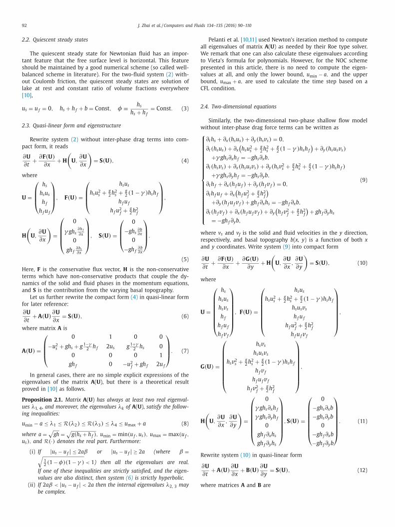
2.3. Quasi-linear form and eigenstructure
Rewrite system (2) without inter-phase drag terms into com-
pact form, it reads
∂U
∂t +
∂F (U )
∂x + H
(U ,
∂U
∂x
)= S (U ) , (4)
where
U =
⎛ ⎜ ⎜ ⎝
h s
h s u s
h f
h f u f
⎞ ⎟ ⎟ ⎠
, F (U ) =
⎛ ⎜ ⎜ ⎝
h s u s
h s u
2 s +
g 2
h
2 s +
g 2 (1 − γ ) h s h f
h f u f
h f u
2 f +
g 2
h
2 f
⎞ ⎟ ⎟ ⎠
,
H
(U ,
∂U
∂x
)=
⎛ ⎜ ⎜ ⎜ ⎝
0
γ gh s ∂h f ∂x
0
gh f ∂h s ∂x
⎞ ⎟ ⎟ ⎟ ⎠
, S (U ) =
⎛ ⎜ ⎜ ⎝
0
−gh s ∂b ∂x
0
−gh f ∂b ∂x
⎞ ⎟ ⎟ ⎠
.
(5)
Here, F is the conservative flux vector, H is the non-conservative
terms which have non-conservative products that couple the dy-
namics of the solid and fluid phases in the momentum equations,
and S is the contribution from the varying basal topography.
Let us further rewrite the compact form (4) in quasi-linear form
for later reference:
∂U
∂t + A (U )
∂U
∂x = S (U ) , (6)
where matrix A is
A (U ) =
⎛ ⎜ ⎜ ⎝
0 1 0 0
−u
2 s + gh s + g 1 −γ
2 h f 2 u s g 1+ γ
2 h s 0
0 0 0 1
gh f 0 −u
2 f + gh f 2 u f
⎞ ⎟ ⎟ ⎠
. (7)
In general cases, there are no simple explicit expressions of the
eigenvalues of the matrix A ( U ), but there is a theoretical result
proved in [10] as follows.
Proposition 2.1. Matrix A ( U ) has always at least two real eigenval-
ues λ1, 4 , and moreover, the eigenvalues λk of A ( U ), satisfy the follow-
ing inequalities:
u min − a ≤ λ1 ≤ R (λ2 ) ≤ R (λ3 ) ≤ λ4 ≤ u max + a (8)
where a =
√
gh =
√
g(h s + h f ) , u min = min (u f , u s ) , u max = max (u f ,
u s ) , and R (·) denotes the real part. Furthermore:
(i) If | u s − u f | ≤ 2 aβ or | u s − u f | ≥ 2 a (where β =√
1 2 (1 − φ)(1 − γ ) < 1 ) then all the eigenvalues are real.
If one of these inequalities are strictly satisfied, and the eigen-
values are also distinct, then system (6) is strictly hyperbolic.
(ii) If 2 aβ < | u s − u f | < 2 a then the internal eigenvalues λ2, 3 may
be complex.
Pelanti et al. [10,11] used Newton’s iteration method to compute
ll eigenvalues of matrix A ( U ) as needed by their Roe type solver.
e remark that one can also calculate these eigenvalues according
o Vieta’s formula for polynomials. However, for the NOC scheme
resented in this article, there is no need to compute the eigen-
alues at all, and only the lower bound, u min − a, and the upper
ound, u max + a, are used to calculate the time step based on a
FL condition.
.4. Two-dimensional equations
Similarly, the two-dimensional two-phase shallow flow model
ithout inter-phase drag force terms can be written as
∂ t h s + ∂ x (h s u s ) + ∂ y (h s v s ) = 0 ,
∂ t (h s u s ) + ∂ x (h s u
2 s +
g 2
h
2 s +
g 2 (1 − γ ) h s h f
)+ ∂ y ( h s u s v s )
+ γ gh s ∂ x h f = −gh s ∂ x b,
∂ t (h s v s ) + ∂ x (h s u s v s ) + ∂ y (h s v 2 s +
g 2
h
2 s +
g 2 (1 − γ ) h s h f )
+ γ gh s ∂ y h f = −gh s ∂ y b,
∂ t h f + ∂ x (h f u f ) + ∂ y (h f v f ) = 0 ,
∂ t h f u f + ∂ x (h f u
2 f +
g 2
h
2 f
)+ ∂ y (h f u f v f ) + gh f ∂ x h s = −gh f ∂ x b,
∂ t (h f v f ) + ∂ x (h f u f v f ) + ∂ y (h f v 2 f +
g 2
h
2 f
)+ gh f ∂ y h s
= −gh f ∂ y b,
(9)
here v s and v f is the solid and fluid velocities in the y direction,
espectively, and basal topography b ( x, y ) is a function of both x
nd y coordinates. Write system (9) into compact form
∂U
∂t +
∂F (U )
∂x +
∂G (U )
∂y + H
(U ,
∂U
∂x , ∂U
∂y
)= S (U ) , (10)
here
=
⎛ ⎜ ⎜ ⎜ ⎜ ⎜ ⎜ ⎝
h s
h s u s
h s v s h f
h f u f
h f v f
⎞ ⎟ ⎟ ⎟ ⎟ ⎟ ⎟ ⎠
, F (U ) =
⎛ ⎜ ⎜ ⎜ ⎜ ⎜ ⎜ ⎝
h s u s
h s u
2 s +
g 2
h
2 s +
g 2 (1 − γ ) h s h f
h s u s v s h f u f
h f u
2 f +
g 2
h
2 f
h f u f v f
⎞ ⎟ ⎟ ⎟ ⎟ ⎟ ⎟ ⎠
,
(U ) =
⎛ ⎜ ⎜ ⎜ ⎜ ⎜ ⎜ ⎜ ⎝
h s v s h s u s v s
h s v 2 s +
g 2
h
2 s +
g 2 (1 − γ ) h s h f
h f v f h f u f v f
h f v 2 f +
g 2
h
2 f
⎞ ⎟ ⎟ ⎟ ⎟ ⎟ ⎟ ⎟ ⎠
,
(U ,
∂U
∂x , ∂U
∂y
)=
⎛ ⎜ ⎜ ⎜ ⎜ ⎜ ⎜ ⎝
0
γ gh s ∂ x h f
γ gh s ∂ y h f
0
gh f ∂ x h s
gh f ∂ y h s
⎞ ⎟ ⎟ ⎟ ⎟ ⎟ ⎟ ⎠
, S (U ) =
⎛ ⎜ ⎜ ⎜ ⎜ ⎜ ⎜ ⎝
0
−gh s ∂ x b
−gh s ∂ y b
0
−gh f ∂ x b
−gh f ∂ y b
⎞ ⎟ ⎟ ⎟ ⎟ ⎟ ⎟ ⎠
. (11)
ewrite system (10) in quasi-linear form
∂U
∂t + A (U )
∂U
∂x + B (U )
∂U
∂y = S (U ) , (12)
here matrices A and B are

J. Zhai et al. / Computers and Fluids 134–135 (2016) 90–110 93
Fig. 1. Sketch of staggered grid for NOC scheme.
A
F
a
a
1
r
w
A
a
s
3
s
fl
p
e
p
n
h
fi
3
s
a
[
r
L
w
s
(∫
D
i
U
t
T
r
T
c
f
t
s
w
(
U
T
f
t
s
o
(U ) =
⎛ ⎜ ⎜ ⎜ ⎜ ⎜ ⎜ ⎜ ⎜ ⎝
0 1 0 0 0 0
−u 2 s + gh s +
g 2 (1 − γ ) h f 2 u s 0 g
2 (1 + γ ) h s 0 0
−u s v s v s u s 0 0 0
0 0 0 0 1 0
gh f 0 0 −u 2 f + gh f 2 u f 0
0 0 0 −u f v f v f u f
⎞ ⎟ ⎟ ⎟ ⎟ ⎟ ⎟ ⎟ ⎟ ⎠
,
B (U ) =
⎛ ⎜ ⎜ ⎜ ⎜ ⎜ ⎜ ⎝
0 0 1 0 0 0
−u s v s v s u s 0 0 0
−v 2 s + gh s +
g 2 (1 − γ ) h f 0 2 v s g
2 (1 + γ ) h s 0 0
0 0 0 0 0 1
0 0 0 −u f v f v f u f
gh f 0 0 −v 2 f + gh f 0 2 v f
⎞ ⎟ ⎟ ⎟ ⎟ ⎟ ⎟ ⎠
.
(13)
rom (13) , it is easy to verify that matrix A has two eigenvalues u s nd u f (see 3rd row and 3rd column, and 6th row and 6th column),
nd the remaining eigenvalues are exactly the same as those in the
d case. Similarly, matrix B has two eigenvalues v s and v f , and the
emaining eigenvalues are analogous to those of matrix A . Hence,
e can continue to make use of Proposition 2.1 for each matrix.
gain, only the lower and upper bounds of the eigenvalues, u min −, u max + a, v min − a, and v max + a, are utilized to calculate the time
tep in the present NOC scheme.
. Non-oscillatory Central Differencing scheme (NOC)
Tai et al. [23,32] and Wang et al. [5] applied the staggered NOC
cheme to numerical simulations of single-phase shallow granular
ows. In this work, we apply the staggered NOC scheme to two-
hase shallow granular flow equations. The well-balanced prop-
rty of the resulting NOC scheme is ensured with a modification
rocedure, and the scheme is proven to be positivity-preserving. A
umerical treatment [31] using the relaxation term to recover the
yperbolicity of the system is adopted to make the scheme work
ne for flow conditions in which the loss of hyperbolicity happens.
.1. One-dimensional NOC scheme
We first illustrate one-dimensional time-space staggered NOC
cheme. As a Godunov method, the solution variables U are the cell
verages on interval [ x i − 1
2 , x
i + 1 2
] at t = t n and on staggered interval
x i , x i +1 ] at t = t n +1 ( Fig. 1 ). With MUSCL reconstruction, one can
econstruct the piecewise linear distribution as
i (x, t n ) = U i (t n ) + ( x − x i ) σn
i , x i − 1 2
≤ x ≤ x i + 1 2 , (14)
�x
here cell average at time t n is defined as U i (t n ) =1
�x
∫ x i + 1 2
x i − 1
2
U (x, t n ) d x, and σn i / �x is the slope and σn
i could be
ome limiter for undivided differences of U i . Integrate system
4) over control volume [ x i , x i +1 ] × [ t n , t n +1 ] as shown in Fig. 2 ,
x i +1
x i
U (x, t n +1 ) d x −∫ x i +1
x i
U (x, t n ) d x
+
∫ t n +1
t n F (x i +1 , t) −
∫ t n +1
t n F (x i , t) d t
= −∫ t n +1
t n
∫ x i +1
x i
H d x d t +
∫ t n +1
t n
∫ x i +1
x i
S d x d t, (15)
ivide Eq. (15) by �x , and define cell average at time t n +1 which
s the unknown solution as
n +1
i + 1 2 =
1
�x
∫ x i +1
x i
U (x, t n +1 ) d x, (16)
hen
1
�x
∫ x i +1
x i
U (x, t n ) d x =
1
�x
[ ∫ x i + 1
2
x i
U (x, t n ) d x +
∫ x i +1
x i + 1
2
U (x, t n ) d x
]
=
1
�x
[ ∫ x i + 1
2
x i
L i (x, t n ) d x +
∫ x i +1
x i + 1
2
L i +1 (x, t n ) d x
]
=
1
2
(U
n
i + U
n
i +1
)+
1
8
(σn
i − σn i +1
). (17)
he time-integration of flux F can be approximated by midpoint
ule of integral ( ◦ points in the right frame of Fig. 2 ),
1
�x
∫ t n +1
t n F (x i +1 , t) d t ≈ �t
�x F
(U
n + 1 2
i +1
),
1
�x
∫ t n +1
t n F (x i , t) d t ≈ �t
�x F
(U
n + 1 2
i
). (18)
o proceed, we need to evaluate the integration of non-
onservative term H ( U, U x ) in Eq. (15) . Because the second and
ourth components of vector H are similar as seen from Eq. (5) , we
ake the fourth component as example. For clarity, we omit con-
tant g . If it is approximated with
1
�x
∫ t n +1
t n
∫ x i +1
x i
h f
∂h s
∂x d x d t ≈ 1
�x
∫ t n +1
t n
(̃ h f ̃
δh s
)i + 1 2
d t
≈ �t
�x
(̃ h f ̃
δh s
)n + 1 2
i + 1 2
=
�t
�x H
n + 1 2
i + 1 2
, (19)
here ( ̃ h f ) n +1 / 2 i +1 / 2
and ( ̃ δh s ) n +1 / 2 i +1 / 2
are suitable approximations to
(h f ) n +1 / 2 i +1 / 2
and (δh s ) n +1 / 2 i +1 / 2
, and if the last bed slope term in Eq.
15) is also discretized properly, then (15) becomes NOC scheme
n +1
i + 1 2 =
1
2
(U
n
i + U
n
i +1
)+
1
8
(σn
i − σn i +1
)− �t
�x
[ F
(U
n + 1 2
i +1
)− F
(U
n + 1 2
i
)] − �t
�x H
n + 1 2
i + 1 2
+
�t
�x S n +
1 2
i + 1 2
. (20)
he RHS of (20) consists of four parts: the quadrature terms
rom the reconstruction (first two terms), the flux terms (third
erm), the nonconservative terms (fourth term), and the bed slope
ource terms (fifth term). As will be shown later, suitable second-
rder discretization schemes for the nonconservative and bed slope
94 J. Zhai et al. / Computers and Fluids 134–135 (2016) 90–110
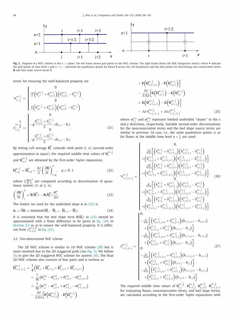
Fig. 2. Diagram of a NOC scheme in the x − t plane. The left frame shows grid points in the NOC scheme. The right frame shows the NOC integration stencil, where • indicate
the grid points at time level n and n + 1 , ◦ represent the quadrature points for fluxes F across the cell boundaries and the data points for discretizing non-conservative terms
H and bed slope source terms S .
w
a
f
s
f
H
S
T
f
a
terms for ensuring the well-balanced property are
H
n + 1 2
i + 1 2
=
⎧ ⎪ ⎪ ⎪ ⎪ ⎨ ⎪ ⎪ ⎪ ⎪ ⎩
0
γ g 2
(h
n + 1 2
s,i + h
n + 1 2
s,i +1
)(h
n + 1 2
f,i +1 − h
n + 1 2
f,i
)0
g 2
(h
n + 1 2
f,i + h
n + 1 2
f,i +1
)(h
n + 1 2
s,i +1 − h
n + 1 2
s,i
) ,
S n +
1
2
i + 1 2
=
⎧ ⎪ ⎪ ⎪ ⎪ ⎪ ⎪ ⎨ ⎪ ⎪ ⎪ ⎪ ⎪ ⎪ ⎩
0
−g h
n + 1 2
s,i +1 + h
n + 1 2
s,i
2
( b i +1 − b i )
0
−g h
n + 1 2
f,i +1 + h
n + 1 2
f,i
2
( b i +1 − b i )
. (21)
By letting cell average U
n
i coincide with point ( i, n ) (second-order
approximation in space), the required middle time values of U
n + 1 2
i
and U
n + 1 2
i +1 are obtained by the first-order Taylor expansions,
U
n + 1 2
i + q = U
n
i + q +
�t
2
(∂U
∂t
)n
i + q , q = 0 , 1 , (22)
where (
∂U ∂t
)n
i are computed according to discretization of quasi-
linear system (6) at ( i, n ), (∂U
∂t
)n
i
= S ( U
n
i ) − A ( U
n
i ) σn
i
�x . (23)
The limiter we used for the undivided slope σ in (23) is
σi = δ̄U i = minmod ( U i − U i −1 , U i +1 − U i ) . (24)
It is remarked that the bed slope term S ( U i ) in (23) should be
approximated with a finite difference to be given in Eq. (34) in
Section 3.3 so as to ensure the well-balanced property. It is differ-
ent from S n +1 / 2 i +1 / 2
in Eq. (21) .
3.2. Two-dimensional NOC scheme
The 2D NOC scheme is similar to 1D NOC scheme (20) but is
more involved due to the 2D staggered grids (see Fig. 3 ). We follow
[5] to give the 2D staggered NOC scheme for system (10) . The final
2D NOC scheme also consists of four parts and is written as
U
n +1
i + 1 2 , j+ 1 2 =
1
4
(U
n
i, j + U
n
i +1 , j + U
n
i, j+1 + U
n
i +1 , j+1
)+
1
16
(σx,n
i, j − σx,n
i +1 , j + σx,n
i, j+1 − σx,n
i +1 , j+1
)+
1
16
(σy,n
i, j − σy,n
i, j+1 + σy,n
i +1 , j − σy,n
i +1 , j+1
)− �t
2�x
[ F
(U
n + 1 2
i +1 , j
)− F
(U
n + 1 2
i, j
)
+ F
(U
n + 1 2
i +1 , j+1
)− F
(U
n + 1 2
i, j+1
)] − �t
2�y
[ G
(U
n + 1 2
i, j+1
)− G
(U
n + 1 2
i, j
)+ G
(U
n + 1 2
i +1 , j+1
)− G
(U
n + 1 2
i +1 , j
)] − �t H
n + 1 2
i + 1 2 , j+ 1 2
+ �t S n + 1 2
i + 1 2 , j+ 1 2
. (25)
here σx,n i, j
and σy,n i, j
represent limited undivided “slopes” in the x
nd y directions, respectively. Suitable second-order discretizations
or the nonconservative terms and the bed slope source terms are
imilar to previous 1d case, i.e., the same quadrature points � as
or fluxes at the middle time level n +
1 2 are used:
n + 1 2
i + 1 2 , j+ 1 2
=
⎧ ⎪ ⎪ ⎪ ⎪ ⎪ ⎪ ⎪ ⎪ ⎪ ⎪ ⎪ ⎪ ⎪ ⎪ ⎪ ⎪ ⎪ ⎪ ⎪ ⎪ ⎪ ⎪ ⎨ ⎪ ⎪ ⎪ ⎪ ⎪ ⎪ ⎪ ⎪ ⎪ ⎪ ⎪ ⎪ ⎪ ⎪ ⎪ ⎪ ⎪ ⎪ ⎪ ⎪ ⎪ ⎪ ⎩
0 ,
γ g 4�x
[ (h
n + 1 2
s,i, j + h
n + 1 2
s,i +1 , j
)(h
n + 1 2
f,i +1 , j − h
n + 1 2
f,i, j
)+
(h
n + 1 2
s,i, j+1 + h
n + 1 2
s,i +1 , j+1
)(h
n + 1 2
f,i +1 , j+1 − h
n + 1 2
f,i, j+1
)] ,
γ g 4�y
[ (h
n + 1 2
s,i, j + h
n + 1 2
s,i, j+1
)(h
n + 1 2
f,i, j+1 − h
n + 1 2
f,i, j
)+
(h
n + 1 2
s,i +1 , j + h
n + 1 2
s,i +1 , j+1
)(h
n + 1 2
f,i +1 , j+1 − h
n + 1 2
f,i +1 , j
)] ,
0 ,
g 4�x
[ (h
n + 1 2
f,i, j + h
n + 1 2
f,i +1 , j
)(h
n + 1 2
s,i +1 , j − h
n + 1 2
s,i, j
)+
(h
n + 1 2
f,i, j+1 + h
n + 1 2
f,i +1 , j+1
)(h
n + 1 2
s,i +1 , j+1 − h
n + 1 2
s,i, j+1
)] ,
g 4�y
[ (h
n + 1 2
f,i, j + h
n + 1 2
f,i, j+1
)(h
n + 1 2
s,i, j+1 − h
n + 1 2
s,i, j
)+
(h
n + 1 2
f,i +1 , j + h
n + 1 2
f,i +1 , j+1
)(h
n + 1 2
s,i +1 , j+1 − h
n + 1 2
s,i +1 , j
)] ,
(26)
n + 1 2
i + 1 2 , j+ 1 2
=
⎧ ⎪ ⎪ ⎪ ⎪ ⎪ ⎪ ⎪ ⎪ ⎪ ⎪ ⎪ ⎪ ⎪ ⎪ ⎪ ⎪ ⎪ ⎪ ⎪ ⎪ ⎪ ⎪ ⎨ ⎪ ⎪ ⎪ ⎪ ⎪ ⎪ ⎪ ⎪ ⎪ ⎪ ⎪ ⎪ ⎪ ⎪ ⎪ ⎪ ⎪ ⎪ ⎪ ⎪ ⎪ ⎪ ⎩
0 ,
− g 4�x
[ (h
n + 1 2
s,i +1 , j+1 + h
n + 1 2
s,i, j+1
)(b i +1 , j+1 − b i, j+1
)+
(h
n + 1 2
s,i +1 , j + h
n + 1 2
s,i, j
)(b i +1 , j − b i, j
)] ,
− g 4�y
[ (h
n + 1 2
s,i +1 , j+1 + h
n + 1 2
s,i +1 , j
)(b i +1 , j+1 − b i +1 , j
)+
(h
n + 1 2
s,i, j+1 + h
n + 1 2
s,i, j
)(b i, j+1 − b i, j
)] ,
0 ,
− g 4�x
[ (h
n + 1 2
f,i +1 , j+1 + h
n + 1 2
f,i, j+1
)(b i +1 , j+1 − b i, j+1
)+
(h
n + 1 2
f,i +1 , j + h
n + 1 2
f,i, j
)(b i +1 , j − b i, j
)] ,
− g 4�y
[ (h
n + 1 2
f,i +1 , j+1 + h
n + 1 2
f,i +1 , j
)(b i +1 , j+1 − b i +1 , j
)+
(h
n + 1 2
f,i, j+1 + h
n + 1 2
f,i, j+1
)(b i, j+1 − b i, j
)] ,
(27)
he required middle time values of U
n + 1 2
i, j , U
n + 1 2
i +1 , j , U
n + 1 2
i, j+1 , U
n + 1 2
i +1 , j+1
or evaluating fluxes, nonconservative terms, and bed slope terms,
re calculated according to the first-order Taylor expansions with
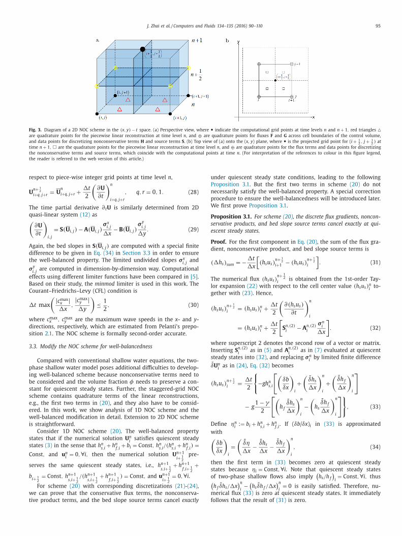
J. Zhai et al. / Computers and Fluids 134–135 (2016) 90–110 95
Fig. 3. Diagram of a 2D NOC scheme in the (x, y ) − t space. (a) Perspective view, where • indicate the computational grid points at time levels n and n + 1 , red triangles �
are quadrature points for the piecewise linear reconstruction at time level n , and � are quadrature points for fluxes F and G across cell boundaries of the control volume,
and data points for discretizing nonconservative terms H and source terms S . (b) Top view of (a) onto the ( x, y ) plane, where • is the projected grid point for ( i +
1 2 , j +
1 2 ) at
time n + 1 , � are the quadrature points for the piecewise linear reconstruction at time level n , and � are quadrature points for the flux terms and data points for discretizing
the nonconservative terms and source terms, which coincide with the computational points at time n . (For interpretation of the references to colour in this figure legend,
the reader is referred to the web version of this article.)
r
U
T
q(A
d
t
σ
e
B
C
�
w
d
s
3
p
i
b
s
s
e
e
w
i
s
s
C
s
b
w
t
u
P
n
p
W
P
s
e
P
d
T
l
g
w
I
s
δ
D
w(t
s
o (
m
f
espect to piece-wise integer grid points at time level n ,
n + 1 2
i + q, j+ r = U
n
i + q, j+ r +
�t
2
(∂U
∂t
)n
i + q, j+ r , q, r = 0 , 1 . (28)
he time partial derivative ∂ t U is similarly determined from 2D
uasi-linear system (12) as
∂U
∂t
)i, j
= S ( U i, j ) − A ( U i, j ) σx
i, j
�x − B ( U i, j )
σy i, j
�y . (29)
gain, the bed slopes in S ( U i, j ) are computed with a special finite
ifference to be given in Eq. (34) in Section 3.3 in order to ensure
he well-balanced property. The limited undivided slopes σx i, j
andy i, j
are computed in dimension-by-dimension way. Computational
ffects using different limiter functions have been compared in [5] .
ased on their study, the minmod limiter is used in this work. The
ourant–Friedrichs–Levy (CFL) condition is
t max
( | c max x | �x
, | c max
y | �y
)≤ 1
2
, (30)
here c max x , c max
y are the maximum wave speeds in the x - and y -
irections, respectively, which are estimated from Pelanti’s prepo-
ition 2.1 . The NOC scheme is formally second-order accurate.
.3. Modify the NOC scheme for well-balancedness
Compared with conventional shallow water equations, the two-
hase shallow water model poses additional difficulties to develop-
ng well-balanced scheme because nonconservative terms need to
e considered and the volume fraction φ needs to preserve a con-
tant for quiescent steady states. Further, the staggered-grid NOC
cheme contains quadrature terms of the linear reconstructions,
.g., the first two terms in (20) , and they also have to be consid-
red. In this work, we show analysis of 1D NOC scheme and the
ell-balanced modification in detail. Extension to 2D NOC scheme
s straightforward.
Consider 1D NOC scheme (20) . The well-balanced property
tates that if the numerical solution U
n i
satisfies quiescent steady
tates (3) in the sense that h n s,i
+ h n f,i
+ b i = Const , h n s,i
/ (h n s,i
+ h n f,i
) =onst , and u
n i
= 0 , ∀ i, then the numerical solution U
n +1
i + 1 2
pre-
erves the same quiescent steady states, i.e., h n +1
s,i + 1 2
+ h n +1
f,i + 1 2
+
i + 1 2
= Const , h n +1
s,i + 1 2
/ (h n +1
s,i + 1 2
+ h n +1
f,i + 1 2
) = Const , and u
n +1
i + 1 2
= 0 , ∀ i .
For scheme (20) with corresponding discretizations (21) - (24) ,
e can prove that the conservative flux terms, the nonconserva-
ive product terms, and the bed slope source terms cancel exactly
nder quiescent steady state conditions, leading to the following
roposition 3.1 . But the first two terms in scheme (20) do not
ecessarily satisfy the well-balanced property. A special correction
rocedure to ensure the well-balancedness will be introduced later.
e first prove Proposition 3.1 .
roposition 3.1. For scheme (20) , the discrete flux gradients, noncon-
ervative products, and bed slope source terms cancel exactly at qui-
scent steady states.
roof. For the first component in Eq. (20) , the sum of the flux gra-
ient, nonconservative product, and bed slope source terms is
( �h s ) sum
= − �t
�x
[ ( h s u s )
n + 1 2
i +1 − ( h s u s )
n + 1 2
i
] . (31)
he numerical flux ( h s u s ) n + 1
2 i
is obtained from the 1st-order Tay-
or expansion (22) with respect to the cell center value (h s u s ) n i to-
ether with (23) . Hence,
(h s u s ) n + 1 2
i = (h s u s )
n i +
�t
2
(∂(h s u s )
∂t
)n
i
= (h s u s ) n i +
�t
2
[S n, (2)
i − A
n, (2) i
σn i
�x
]. (32)
here superscript 2 denotes the second row of a vector or matrix.
nserting S n, (2) i
as in (5) and A
n, (2) i
as in (7) evaluated at quiescent
teady states into (32) , and replacing σn i
by limited finite difference
¯U
n i
as in (24) , Eq. (32) becomes
(h s u s ) n + 1 2
i =
�t
2
{
−gh
n s,i
[ (δb
δx
)i
+
(δ̄h s
�x
)n
i
+
(δ̄h f
�x
)n
i
]
− g 1 − γ
2
[ (h f
δ̄h s
�x
)n
i
−(
h s
δ̄h f
�x
)n
i
] }
, (33)
efine ηn i
:= b i + h n s,i
+ h n f,i
. If ( δb / δx ) i in (33) is approximated
ith
δb
δx
)i
=
(δ̄η
�x − δ̄h s
�x − δ̄h f
�x
)n
i
, (34)
hen the first term in (33) becomes zero at quiescent steady
tates because ηi = Const , ∀ i . Note that quiescent steady states
f two-phase shallow flows also imply (h s /h f
)i = Const , ∀ i, thus
h f δ̄h s / �x )n
i −
(h s ̄δh f / �x
)n
i = 0 is easily satisfied. Therefore, nu-
erical flux (33) is zero at quiescent steady states. It immediately
ollows that the result of (31) is zero.
96 J. Zhai et al. / Computers and Fluids 134–135 (2016) 90–110
c
t
e
t
c
f
t
s
g
(
t
n
a
h
W
i
t
g
h
S
i
c
fi
c
t
f
i
r
s
t
s
t
Consequently, the conclusion for the first component of scheme
(20) is proved. In a similar way, it is easy to prove the third com-
ponent of (20) .
Before we prove the more involved second and fourth compo-
nents of (20) , we note that for quiescent steady states, Taylor ex-
pansion (22) together with (23) gives
(h s ) n + 1 2
i = (h s )
n i +
1
2
�t
(∂h s
∂t
)n
i
= (h s ) n i +
1
2
�t
(− δ̄( hu s )
�x
)n
i
= (h s ) n i , (35)
and similarly, (h f ) n + 1
2 i
= (h f ) n i . As the fourth component is simpler
than the second component, we start from the fourth component.
Using quiescent steady states and discretization (21) , the sum of
the discrete flux gradient, nonconservative product, and bed slope
source terms for the fourth component is
�(h f u f ) sum
= −�t
⎧ ⎨ ⎩
(g 2
h
2 f
)n + 1 2
i +1 −
(g 2
h
2 f
)n + 1 2
i
�x + g
(h
n + 1 2
f,i +1 + h
n + 1 2
f,i
)h
n + 1 2
s,i +1 − h
n + 1 2
s,i
2�x
+ g
(h
n + 1 2
f,i +1 + h
n + 1 2
f,i
)b n + 1 2
s,i +1 − b
n + 1 2
s,i
2�x
}
. (36)
Notice that since h n + 1
2
s, f = h n
s, f , we omit sup-script n +
1 2 and extract
the factor g /2 �x out of the big bracket. Then the remaining part
becomes (h
2 f,i +1 − h
2 f,i
)+ (h f,i +1 + h f,i ) ( h s,i +1 − h s,i )
+(h f,i +1 + h f,i ) ( b i +1 − b i )
=
(h
2 f,i +1 − h
2 f,i
)+ (h f,i +1 + h f,i ) ( h s,i +1 − h s,i + b i +1 − b i )
=
(h
2 f,i +1 − h
2 f,i
)+ (h f,i +1 + h f,i )( const − h f,i +1 − const + h f,i )
= 0 . (37)
Similarly, for the second component in (20) , the sum can be writ-
ten as
�(h s u s ) sum
�t
= −(
g 2
h
2 s +
g 2 (1 − γ ) h s h f
)n + 1 2
i +1 −
(g 2
h
2 s +
g 2 (1 − γ ) h s h f
)n + 1 2
i
�x
−γ g(h
n + 1 2
s,i +1 + h
n + 1 2
s,i )
h
n + 1 2
f,i +1 − h
n + 1 2
f,i
2�x − g(h
n + 1 2
s,i +1 + h
n + 1 2
s,i )
b i +1 − b i 2�x
(38)
Again, omit superscript n +
1 2 and extract the factor −g/ 2�x, the
RHS of (38) reduces to (h
2 s,i +1 − h
2 s,i
)+ (1 − γ )
(h s,i +1 h f,i +1 − h s,i h f,i
)+ γ (h s,i +1 + h s,i )
(h f,i +1 − h f,i
)+ (h s,i + h s,i +1 ) ( b i +1 − b i )
=
(h
2 s,i +1 − h
2 s,i
)+ (1 − γ )
(h s,i +1 h f,i +1 − h s,i h f,i
)+(γ − 1)(h s,i +1 + h s,i )
(h f,i +1 − h f,i
)+(h s,i + h s,i +1 )
(h f,i +1 − h f,i + b i +1 − b i
)=
(h
2 s,i +1 − h
2 s,i
)+ (1 − γ )
(h s,i +1 h f,i − h s,i h f,i +1
)+(h s,i + h s,i +1 ) ( const − h s,i +1 − const + h s,i )
= (1 − γ ) (h s,i +1 h f,i − h s,i h f,i +1
)= 0 , (39)
where the last equality results from the condition (h s /h f ) i =onst , ∀ i .
In summary, the sum of discrete flux terms, nonconservative
erms and topography source terms in scheme (20) is zero at qui-
scent steady states. This ends the proof. �
Next, we consider how to make the results from the first two
erms in scheme (20) , i.e., the quadrature terms for the linear re-
onstructions, satisfy the well-balanced property. The second and
ourth components of the two terms at quiescent steady states give
he solid and fluid momentums,
( h s u s ) n +1
i + 1 2
=
1
2
[(h s u s )
n i + (h s u s )
n i +1
]+
1
8
(σn, (2)
i − σn, (2)
i +1
),
( h f u f ) n +1
i + 1 2
=
1
2
[(h f u f )
n i + (h f u f )
n i +1
]+
1
8
(σn, (4)
i − σn, (4)
i +1
). (40)
ince u
n i
= 0 , ∀ i, all terms in the RHS of (40) are equal to zero,
iving h u
n +1
i + 1 2
= 0 so that the first item of well-balanced condition
3) is satisfied. But the first and third components of the first two
erms in (20) need special treatment. The first and third compo-
ents of the two terms at quiescent steady states give the solid
nd fluid heights,
h
n +1
s,i + 1 2
=
1
2
(h
n s,i + h
n s,i +1
)+
1
8
(σn, (1)
i − σn, (1)
i +1
),
n +1
f,i + 1 2
=
1
2
(h
n f,i + h
n f,i +1
)+
1
8
(σn, (3)
i − σn, (3)
i +1
). (41)
ith
(h s /h f
)n
i = Const , it is easy to show the results from (41) sat-
sfy (h s /h f
)n +1
i + 1 2
= Const , thus the last item of well-balanced condi-
ion (3) is satisfied. However, the new free surface level at a stag-
ered gird point as calculated from (41) is
n +1
s,i + 1 2
+ h
n +1
f,i + 1 2
+ b i + 1 2
=
1
2
[(h
n s,i + h
n f,i + b i
)+
(h
n s,i +1 + h
n f,i +1 + b i +1
)]+
1
8
(σn, (1)
i + σn, (3)
i − σn, (1)
i +1 − σn, (3)
i +1
)+ b i + 1 2
− 1
2
( b i + b i +1 )
= Const +
1
8
(σn, (1)
i + σn, (3)
i − σn, (1)
i +1 − σn, (3)
i +1
)−1
2
( b i + b i +1 ) + b i + 1 2 . (42)
ince h n s,i
and h n f,i
may vary from point to point, the second term
n the second equality of (42) are not zero in general, and this may
ause h n +1
s,i + 1 2
+ h n +1
f,i + 1 2
+ b i + 1
2 = Const if b i , b i +1 and b
i + 1 2
are prede-
ned irrespective of the flow solution. We give a modification pro-
edure to cure this problem.
Modification procedure for well-balancedness . This modifica-
ion makes use of the fact that the total mass equation using the
ree surface level η = h s + h f + b as solution variable can automat-
cally ensure the solution of lake at rest [33] , where basal topog-
aphy b is assumed to be time-independent. It only modifies the
olid and fluid heights as computed from the first and third equa-
ions of scheme (20) .
To avoid confusion, the following variables are not quiescent
teady states. By adding the two mass equations in Eq. (2) , we ob-
ain the total mass equation
∂η
∂t +
∂ (h s u s + h f u f
)∂x
= 0 . (43)

J. Zhai et al. / Computers and Fluids 134–135 (2016) 90–110 97
B
p
η
w
t
z
q
f
h
h
h
e
s
b
a
n
t
s
h
3
d
P
(
p
�
w
U
P
t
N
h
w
T
(
h
B
w
o
n
W
s
t
a
�
T
3
(
e
m
a
s
p
P
w
m
I
r
T
u
u
y applying NOC scheme (20) to (43) , we additionally com-
ute the free surface level
n +1
i + 1 2
=
1
2
(ηn
i + ηn i +1
)+
1
8
(σn, (η)
i − σn, (η)
i +1
)− �t
�x
[ (h s u s + h f u f
)n + 1 2
i +1 −
(h s u s + h f u f
)n + 1 2
i
] , (44)
here σn, (η) i
is limited difference of ηn i
= h n s,i
+ h n f,i
+ b i . According
o previous analysis in Proposition 3.1 , the mass fluxes in (44) are
ero for quiescent steady states, thus (44) satisfies ηn +1
i + 1 2
= Const at
uiescent steady states. In general cases, variable ηn + 1
2
i + 1 2
computed
rom (44) is used to modify the solid and fluid heights h n +1
s,i + 1 2
and
n +1
f,i + 1 2
computed from scheme (20) in the following way:
if ( h n +1
s,i + 1 2
+ h n +1
f,i + 1 2
+ b i + 1
2 = ηn +1
i + 1 2
) then
n +1 , mod
s,i + 1 2
=
h
n +1
s,i + 1 2
h
n +1
s,i + 1 2
+ h
n +1
f,i + 1 2
×(ηn +1
i + 1 2
− b i + 1 2
),
n +1 , mod
f,i + 1 2
=
h
n +1
f,i + 1 2
h
n +1
s,i + 1 2
+ h
n +1
f,i + 1 2
×(ηn +1
i + 1 2
− b i + 1 2
), (45)
lse no modification is made to h n + 1
2
s,i + 1 2
and h n + 1
2
f,i + 1 2
as computed from
cheme (20) .
The topography b i + 1
2 in (45) can be defined as b
i + 1 2
=
1 2 (b i +
i +1 ) or z b (x i +1 / 2
)and never changes with time stepping. The solid
nd fluid heights after modification (45) are then used as the fi-
al solution for (n + 1) th time step. It is seen that (45) leads
o h n +1 , mod
s,i + 1 2
+ h n +1 , mod
f,i + 1 2
+ b i + 1
2 = ηn +1
i + 1 2
, which can keep the con-
tant at quiescent steady states. And the ratio h n +1 , mod
s,i + 1 2
/h n +1 , mod
f,i + 1 2
=
n +1
s,i + 1 2
/h n +1
f,i + 1 2
= Const is reserved.
.4. Positivity preserving
We can prove that NOC scheme (20) is positivity-preserving un-
er a suitable CFL condition.
roposition 3.2. Assume that system (2) is solved with NOC scheme
20) and that h n s,i
≥ 0 , h n f,i
≥ 0 , ∀ i. Then h n +1
s,i + 1 2
≥ 0 , h n +1
f,i + 1 2
≥ 0 , ∀ i,
rovided that
t ≤ �x min
(CFL
S , 1
4 U
)(46)
here
= max i
(max (| u
n s,i | , | u
n f,i | )
),
S = max i
(∣∣∣max (u
n s,i , u
n f,i ) +
√
g(h
n s,i
+ h
n f,i
)
∣∣∣, ∣∣∣min (u
n s,i , u
n f,i ) −
√
g(h
n s,i
+ h
n f,i
)
∣∣∣). (47)
roof. Since the mass equations of fluid and solid are similar, we
ake the fluid mass equation as example. The third component of
OC scheme (20) gives
n +1
f,i + 1 2
=
1
2
(h
n f,i +
1
4
δ̄h
n f,i + h
n f,i +1 −
1
4
δ̄h
n f,i +1
)− �t
�x
[ (h f u f )
n + 1 2
i +1 − (h f u f )
n + 1 2
i
] , (48)
here δ̄h n f,i
represents the limited difference. The numerical flux
(h f u f ) n +1 / 2 i
is computed according Taylor expansion (22) ,
(h f u f ) n + 1 2
i = (h f u f )
n i +
�t
2
∂(h f u f )
∂t
∣∣∣∣n
i
. (49)
he second term can be ignored as it is O(�t) higher. Hence,
48) can be rewritten as
n +1
f,i + 1 2
=
1
2
[h
n f,i +
1
4
δ̄h
n f,i +
2�t
�x
(h f u f
)n
i
]+
1
2
[h
n f,i +1 −
1
4
δ̄h
n f,i +1 −
2�t
�x
(h f u f
)n
i +1
]=
1
2
[1
2
(h
n f,i +
1
2
δ̄h
n f,i
)+ h
n f,i
(1
2
+
2�tu
n f,i
�x
)]+
1
2
[1
2
(h
n f,i +1 −
1
2
δ̄h
n f,i +1
)+ h
n f,i +1
(1
2
−2�tu
n f,i +1
�x
)](50)
ased on the monotonicity of the minmod-MUSCL interpolation,
e have h n f,i
+
1 2 δ̄h n
f,i ≥ 0 and h n
f,i +1 − 1
2 δ̄h n f,i +1
≥ 0 if h n f,i
≥ 0 , ∀ i . In
rder to make the second terms in the square brackets in (50) be
on-negative, time step �t must satisfy
�t| u
n f,i |
�x ≤ 1
4
, ∀ i. (51)
ith (51) holding, the result of (50) is non-negative. A similar time
tep constraint can also be obtained for the solid phase.
It is evident that (46) is the minimal time step constrained by
he positivity preserving condition (51) for fluid and solid phases
nd by the original CFL condition of NOC scheme,
t = CFL �x
S . (52)
herefore, if (46) is satisfied, then h n +1
s,i + 1 2
≥ 0 , h n +1
f,i + 1 2
≥ 0 , ∀ i . �
.5. Numerical treatment for the loss of hyperbolicity
Although NOC scheme (20) with well-balanced correction
45) is stable even if the matrices of the system have complex
igenvalues, strong unphysical oscillations may appear in the nu-
erical solutions when the modulus of the complex eigenvalues
re big enough. Therefore, we adopt a similar predictor/corrector
trategy [31] to recover the hyperbolic nature of the two-
hase shallow-water system once the necessary condition (ii) of
roposition 2.1 is present. The predictor step is scheme (20) with
ell-balanced correction (45) , which gives the first set of approxi-
ations at time t n +1 , U
n +1 , ∗ = [ h n +1 , ∗s,i
, h n +1 , ∗f,i
, (hu ) n +1 , ∗s,i
, (hu ) n +1 , ∗f,i
] T .
n the corrector step, the state U
n +1 is computed by a numerical
elaxation procedure
h
n +1 s,i
= h
n +1 , ∗s,i
,
h
n +1 f,i
= h
n +1 , ∗f,i
,
( hu ) n +1 s,i = ( hu )
n +1 , ∗s,i + γ�tD
n +1 i
(h
n +1 s,i
+ h
n +1 f,i
)(u
n +1 f,i
− u
n +1 s,i
),
( hu ) n +1 f,i = ( hu )
n +1 , ∗f,i − �tD
n +1 i
(h
n +1 s,i
+ h
n +1 f,i
)(u
n +1 f,i
− u
n +1 s,i
). (53)
he last two equations in (53) are rewritten as follows
n +1 s,i
= u
n +1 , ∗s,i
+
γ�tD
n +1 i
(h
n +1 s,i
+ h
n +1 f,i
)h
n +1 s,i
(u
n +1 f,i
− u
n +1 s,i
),
n +1 f,i
= u
n +1 , ∗f,i
−�tD
n +1 i
(h
n +1 s,i
+ h
n +1 f,i
)h
n +1 f,i
(u
n +1 f,i
− u
n +1 s,i
). (54)
98 J. Zhai et al. / Computers and Fluids 134–135 (2016) 90–110
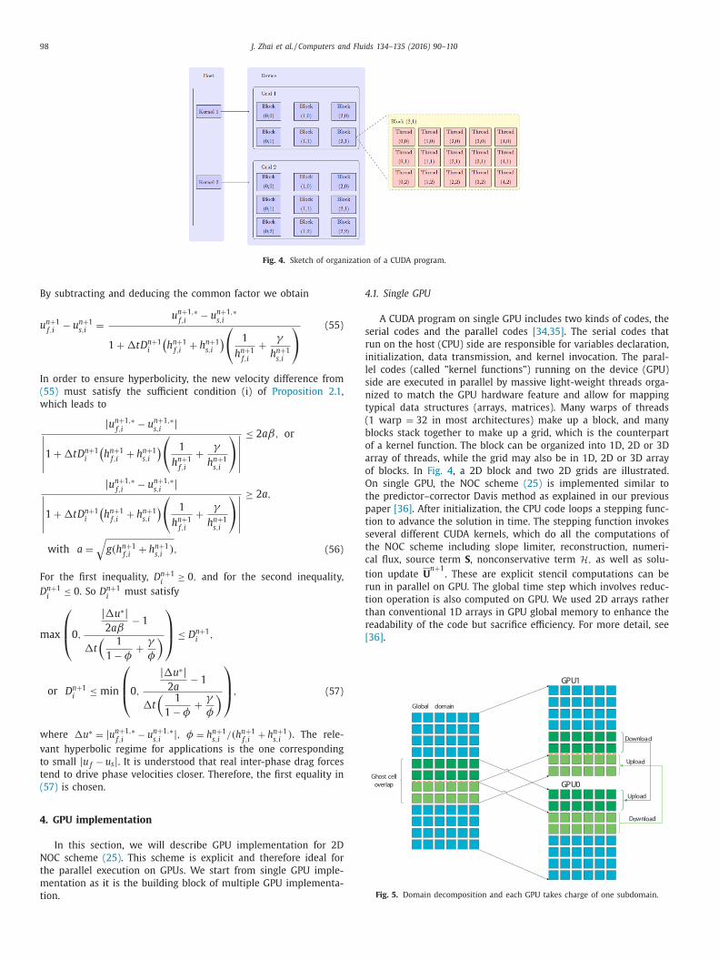
Fig. 4. Sketch of organization of a CUDA program.
4
s
r
i
l
s
n
t
(
b
o
a
o
O
t
p
t
s
t
c
t
r
t
t
r
[
Ghost celloverlap
Global domain
GPU1
GPU0
Dow nload
Upload
Download
Upload
Fig. 5. Domain decomposition and each GPU takes charge of one subdomain.
By subtracting and deducing the common factor we obtain
u
n +1 f,i
− u
n +1 s,i
=
u
n +1 , ∗f,i
− u
n +1 , ∗s,i
1 + �tD
n +1 i
(h
n +1 f,i
+ h
n +1 s,i
)(
1
h
n +1 f,i
+
γ
h
n +1 s,i
) (55)
In order to ensure hyperbolicity, the new velocity difference from
(55) must satisfy the sufficient condition (i) of Proposition 2.1 ,
which leads to
| u
n +1 , ∗f,i
− u
n +1 , ∗s,i
| ∣∣∣∣∣1 + �tD
n +1 i
(h
n +1 f,i
+ h
n +1 s,i
)(
1
h
n +1 f,i
+
γ
h
n +1 s,i
)
∣∣∣∣∣≤ 2 aβ, or
| u
n +1 , ∗f,i
− u
n +1 , ∗s,i
| ∣∣∣∣∣1 + �tD
n +1 i
(h
n +1 f,i
+ h
n +1 s,i
)(
1
h
n +1 f,i
+
γ
h
n +1 s,i
)
∣∣∣∣∣≥ 2 a,
with a =
√
g(h
n +1 f,i
+ h
n +1 s,i
) , (56)
For the first inequality, D
n +1 i
≥ 0 , and for the second inequality,
D
n +1 i
≤ 0 . So D
n +1 i
must satisfy
max
⎛ ⎜ ⎝
0 ,
| �u
∗| 2 aβ
− 1
�t
(1
1 − φ+
γ
φ
)⎞ ⎟ ⎠
≤ D
n +1 i
,
or D
n +1 i
≤ min
⎛ ⎜ ⎝
0 ,
| �u
∗| 2 a
− 1
�t
(1
1 − φ+
γ
φ
)⎞ ⎟ ⎠
, (57)
where �u ∗ = | u n +1 , ∗f,i
− u n +1 , ∗s,i
| , φ = h n +1 s,i
/ (h n +1 f,i
+ h n +1 s,i
) . The rele-
vant hyperbolic regime for applications is the one corresponding
to small | u f − u s | . It is understood that real inter-phase drag forces
tend to drive phase velocities closer. Therefore, the first equality in
(57) is chosen.
4. GPU implementation
In this section, we will describe GPU implementation for 2D
NOC scheme (25) . This scheme is explicit and therefore ideal for
the parallel execution on GPUs. We start from single GPU imple-
mentation as it is the building block of multiple GPU implementa-
tion.
.1. Single GPU
A CUDA program on single GPU includes two kinds of codes, the
erial codes and the parallel codes [34,35] . The serial codes that
un on the host (CPU) side are responsible for variables declaration,
nitialization, data transmission, and kernel invocation. The paral-
el codes (called ”kernel functions”) running on the device (GPU)
ide are executed in parallel by massive light-weight threads orga-
ized to match the GPU hardware feature and allow for mapping
ypical data structures (arrays, matrices). Many warps of threads
1 warp = 32 in most architectures) make up a block, and many
locks stack together to make up a grid, which is the counterpart
f a kernel function. The block can be organized into 1D, 2D or 3D
rray of threads, while the grid may also be in 1D, 2D or 3D array
f blocks. In Fig. 4 , a 2D block and two 2D grids are illustrated.
n single GPU, the NOC scheme (25) is implemented similar to
he predictor–corrector Davis method as explained in our previous
aper [36] . After initialization, the CPU code loops a stepping func-
ion to advance the solution in time. The stepping function invokes
everal different CUDA kernels, which do all the computations of
he NOC scheme including slope limiter, reconstruction, numeri-
al flux, source term S , nonconservative term H, as well as solu-
ion update U
n +1 . These are explicit stencil computations can be
un in parallel on GPU. The global time step which involves reduc-
ion operation is also computed on GPU. We used 2D arrays rather
han conventional 1D arrays in GPU global memory to enhance the
eadability of the code but sacrifice efficiency. For more detail, see
36] .

J. Zhai et al. / Computers and Fluids 134–135 (2016) 90–110 99
Table 1
Comparison of running times using OpenMP-CUDA and multistream-CUDA for 1–3
GPUs with meshes 200 × 200 and 800 × 800 respectively. Result using a CPU with
OpenMP is also shown.
Number of GPUs n x × n y OpenMP-CUDA Multistream-CUDA
1 200 × 200 2478 ms
800 × 800 115938 ms
2 200 × 200 2080 ms 2190 ms
800 × 800 68799 ms 68200 ms
3 200 × 200 2035 ms 2260 ms
800 × 800 51523 ms 49980 ms
10 cores CPU 200 × 200 7354 ms
800 × 800 492586 ms
4
c
v
m
m
i
m
c
i
m
m
e
i
p
i
i
g
a
s
t
c
l
T
d
e
c
P
1
2
3
4
5
6
7
8
9
1
1
M
1
2
3
4
F
r
.2. Multiple GPUs
For using multiple GPUs in a single node, there are several
hoices of strategies. One can use multistream technique pro-
ided by CUDA, or multiple threads with OpenMP (or Pthread), or
essage passing interface (MPI), with each stream/thread/process
anaging a GPU executing a partitioned task. The MPI approach
s mainly suited to GPU clusters, so in this work, we only imple-
ent the OpenMP-CUDA and the multistream-CUDA strategies and
ompare their performances. The computational domain is divided
nto multiple subdomains for multiple GPUs to handle. The subdo-
ains have an overlap of four ghost cells for the purpose of com-
unication, two from each of the neighboring subdomains, as ex-
mplified in Fig. 5 . In the OpenMP-CUDA strategy, as the code runs
n the OpenMP parallel region , the main program spawns multi-
le threads equal to the number of subdomains, and each thread
s attached to a GPU that initializes and computes a correspond-
ng subdomain. In the multistream-CUDA strategy, the main pro-
ram issues multiple streams in turn, and each stream attaches to
GPU. The OpenMP-CUDA strategy is shown in procedure 1. It is
een that there is no need to do initialization in CPU and copy data
o GPU. But device synchronization is performed after step 6 for
alculating a global time step and in step 8 for exchanging over-
apped cells between GPUs (“download” and “upload” in Fig. 5 ).
he multistream-CUDA strategy is shown in procedure 2. The only
ifference between the two strategies is that the starting of GPU
xecution is synchronous in the OpenMP strategy while it is asyn-
hronous in the multistream strategy.
rocedure 1. OpenMP-CUDA procedure:
: Set the number of OMP threads and the same number of GPU de-
vices.
: � pragma omp parallel shared ( �t, ghost variables...) { /* Start parallel region executed by OpenMP threads. Declare
ghost variables as shared variables in order to transfer data be-
tween GPUs. */
ig. 6. Simple Riemann problem. Results computed with 100 grid cells (symbols) are com
epresent the initial conditions.
: Each OpenMP thread binds with a GPU device, allocate the shared
variables, and initialize a subdomain, e.g. the current thread k =omp get thread num ( void ) will take charge of a subdomain with
index (b x , b y ) for the 2D decomposition of the computational
domain being
(b x , b y ) = (k % OMPthreadnumber x ,
k % OMPthreadnumber y )
: InitCon <<< BLOCKs, THREADs >>> (variable list including GPU id
k )
/* This kernel function computes initial conditions; run in parallel
on all GPUs. Need not copy data to GPU. */
: while (T < totaltime) do
: Execute getdeltat <<< BLOCKs, THREADs >>> (variable list including
GPU id k )
/* this kernel returns �t(k ) of each subdomain. Subsequently,
synchronize all threads and then apply Op enMP reduce op eration
to all threads’ �t(k ) to get a minimum �t of the whole domain.
*/
: Execute kernels for the NOC formula (25) to compute solution vari-
ables.
: Synchronize all threads, and then exchange the ghost variables be-
tweenGPUs. Can use the p eer-to-p eer function to exchange data
in new device like K40 GPU used in this work.
: enddo while
0: Copy data back to CPU and write the data file.
1: } // end of OMP parallel region
ultiStream-CUDA procedure:
: Set the number of streams and the same number of GPU devices.
: Use for loop to create stream, and define variables and allocate cor-
responding global memories on each GPU device corresponding
to each stream.
/* Streams are created serially but execute own contexts in par-
allel asynchronously */
: Each stream executes InitCon <<< BLOCKs, THREADs, 0,
stream[k] >>> (variable list)on kth GPU.
/* This is done in a for loop , but streams managing
corresponding GPUs run in parallel and asynchronously. */
: while T < totltime) do
pared with reference solution obtained with 10 0 0 cells (solid lines). Dashed lines
100 J. Zhai et al. / Computers and Fluids 134–135 (2016) 90–110
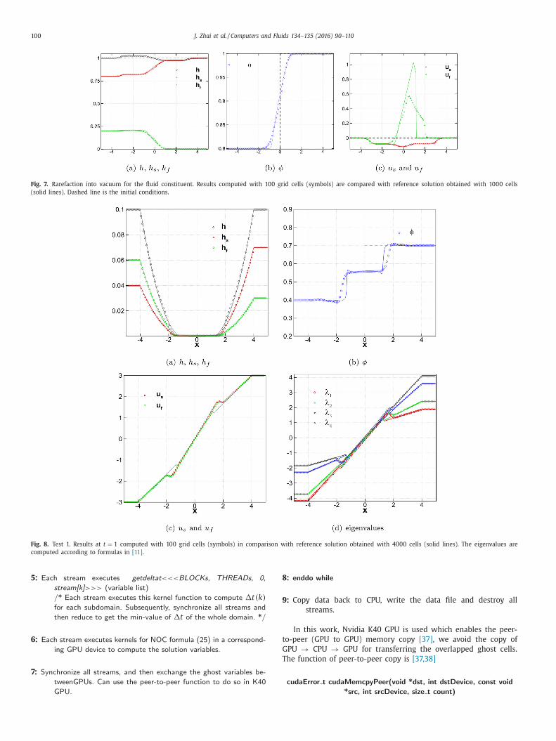
Fig. 7. Rarefaction into vacuum for the fluid constituent. Results computed with 100 grid cells (symbols) are compared with reference solution obtained with 10 0 0 cells
(solid lines). Dashed line is the initial conditions.
Fig. 8. Test 1. Results at t = 1 computed with 100 grid cells (symbols) in comparison with reference solution obtained with 40 0 0 cells (solid lines). The eigenvalues are
computed according to formulas in [11] .
8
9
t
G
T
5: Each stream executes getdeltat <<< BLOCKs, THREADs, 0,
stream[k] >>> (variable list)
/* Each stream executes this kernel function to compute �t(k )
for each subdomain. Subsequently, synchronize all streams and
then reduce to get the min-value of �t of the whole domain. */
6: Each stream executes kernels for NOC formula (25) in a correspond-
ing GPU device to compute the solution variables.
7: Synchronize all streams, and then exchange the ghost variables be-
tweenGPUs. Can use the p eer-to-p eer function to do so in K40
GPU.
: enddo while
: Copy data back to CPU, write the data file and destroy all
streams.
In this work, Nvidia K40 GPU is used which enables the peer-
o-peer (GPU to GPU) memory copy [37] , we avoid the copy of
PU → CPU → GPU for transferring the overlapped ghost cells.
he function of peer-to-peer copy is [37,38]
cudaError t cudaMemcpyPeer(void *dst, int dstDevice, const void
*src, int srcDevice, size t count)
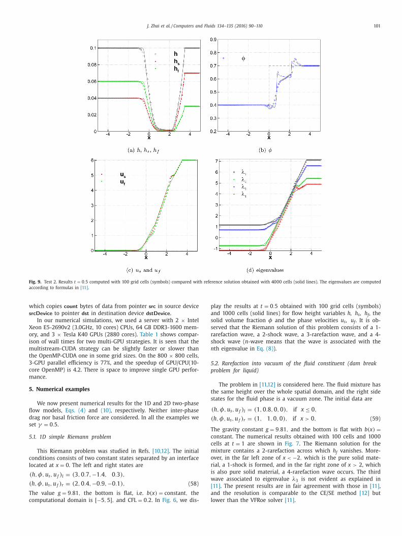
J. Zhai et al. / Computers and Fluids 134–135 (2016) 90–110 101
Fig. 9. Test 2. Results t = 0 . 5 computed with 100 grid cells (symbols) compared with reference solution obtained with 40 0 0 cells (solid lines). The eigenvalues are computed
according to formulas in [11] .
w
s
X
o
i
m
t
3
c
m
5
fl
d
s
5
c
l
T
c
p
a
s
s
r
s
n
5
p
t
s
T
c
c
m
o
r
i
w
[
a
l
hich copies count bytes of data from pointer src in source device
rcDevice to pointer dst in destination device dstDevice .
In our numerical simulations, we used a server with 2 × Intel
eon E5-2690v2 (3.0GHz, 10 cores) CPUs, 64 GB DDR3-1600 mem-
ry, and 3 × Tesla K40 GPUs (2880 cores). Table 1 shows compar-
son of wall times for two multi-GPU strategies. It is seen that the
ultistream-CUDA strategy can be slightly faster or slower than
he OpenMP-CUDA one in some grid sizes. On the 800 × 800 cells,
-GPU parallel efficiency is 77%, and the speedup of GPU/CPU(10-
ore OpenMP) is 4.2. There is space to improve single GPU perfor-
ance.
. Numerical examples
We now present numerical results for the 1D and 2D two-phase
ow models, Eqs. (4) and (10) , respectively. Neither inter-phase
rag nor basal friction force are considered. In all the examples we
et γ = 0 . 5 .
.1. 1D simple Riemann problem
This Riemann problem was studied in Refs. [10,12] . The initial
onditions consists of two constant states separated by an interface
ocated at x = 0 . The left and right states are
(h, φ, u s , u f ) l = (3 , 0 . 7 , −1 . 4 , 0 . 3) ,
(h, φ, u s , u f ) r = (2 , 0 . 4 , −0 . 9 , −0 . 1) , (58)
he value g = 9 . 81 , the bottom is flat, i.e. b(x ) = constant , the
omputational domain is [ −5 , 5] , and CFL = 0 . 2 . In Fig. 6 , we dis-
lay the results at t = 0 . 5 obtained with 100 grid cells (symbols)
nd 10 0 0 cells (solid lines) for flow height variables h, h s , h f , the
olid volume fraction φ and the phase velocities u s , u f . It is ob-
erved that the Riemann solution of this problem consists of a 1-
arefaction wave, a 2-shock wave, a 3-rarefaction wave, and a 4-
hock wave ( n - wave means that the wave is associated with the
th eigenvalue in Eq. (8) ).
.2. Rarefaction into vacuum of the fluid constituent (dam break
roblem for liquid)
The problem in [11,12] is considered here. The fluid mixture has
he same height over the whole spatial domain, and the right side
tates for the fluid phase is a vacuum zone. The initial data are
(h, φ, u s , u f ) l = (1 , 0 . 8 , 0 , 0) , if x ≤ 0 ,
(h, φ, u s , u f ) r = (1 , 1 , 0 , 0) , if x > 0 , (59)
he gravity constant g = 9 . 81 , and the bottom is flat with b(x ) =onstant . The numerical results obtained with 100 cells and 10 0 0
ells at t = 1 are shown in Fig. 7 . The Riemann solution for the
ixture contains a 2-rarefaction across which h f vanishes. More-
ver, in the far left zone of x < −2 , which is the pure solid mate-
ial, a 1-shock is formed, and in the far right zone of x > 2, which
s also pure solid material, a 4-rarefaction wave occurs. The third
ave associated to eigenvalue λ3 is not evident as explained in
11] . The present results are in fair agreement with those in [11] ,
nd the resolution is comparable to the CE/SE method [12] but
ower than the VFRoe solver [11] .

102 J. Zhai et al. / Computers and Fluids 134–135 (2016) 90–110
Fig. 10. Test 3. Results t = 0 . 5 computed with 100 grid cells (symbols) compared with reference solution obtained with 40 0 0 cells (solid lines). The eigenvalues are computed
according to formulas in [11] .
Table 2
Initial data for the test cases of dry bed formation.
Test ( h, φ, u s , u f ) l ( h, φ, u s , u f ) r
1 (0.1, 0.4, −3, −3) (0.1, 0.7, 3, 3)
2 (0.1, 0.4, 0, 0) (0.1, 0.7, 6, 6)
3 (0.2, 0.4, −3, −3) (0.1, 0.8, 3, 3)
Fig. 11. Initial conditions for the numerical test of perturbation of a steady state at
rest. Left: total flow height h + b, Right: solid volume fraction φ. (Here ̃ h and ˜ φ are
made much larger than the values used in the calculation in order to make it clear
for the readers.)
h
t
u
[
t
5.3. Dry bed generation
This problem in [11,12] is concerned with the formation of a
dry bed zone. Three test cases of the Riemann problems are con-
sidered. The solutions consist of two opposite moving rarefaction
fans between which a dry bed region is generated. The initial data
are given in Table 2 :
In all test cases, the initial interface is located at x = 0 and
the bottom is constant, i.e. b(x ) = constant . The computational do-
main is [ −5 , 5] , CFL = 0 . 5 , and g = 9 . 81 . Our model is the same as
[12] in that no inter-phase drag is used whereas [11] used infinitely
large drag force so that so that | u s − u f | is instantaneously driven
to zero. Figs. 8 –10 display results at t = 1 , t = 0 . 5 , t = 0 . 5 for the
three cases, respectively.
In Fig. 8 we display for test 1 the plots of the flow height h, h s ,
h f , solid volume fraction φ, velocities u s , u f , and the four eigen-
values λ1 , λ2 , λ3 , λ4 of matrix A in (7) , respectively. As the fluids
separate outward at x = 0 , a region of vacuum is generated. From
Fig. 8 (a) it is seen that both 40 0 0 grid cells (solid lines) and 100
grid cells (symbols) capture a vacuum region (defined as where
< 10 −5 ) . The distribution of the solid fraction and velocity inside
his vacuum region may be abnormal but we plot them in the vac-
um region for completeness rather than leaving them blank as in
11] . We can see that there are overshot and undershot in φ near
he edges of the vacuum region, but they diminish for 40 0 0 cells.

J. Zhai et al. / Computers and Fluids 134–135 (2016) 90–110 103
Fig. 12. Perturbation of a steady state at rest( ̃ h =
˜ φ = 10 −3 ). Circles: solution computed with 200 grid cells; solid line: reference solution computed with 30 0 0 grid cells. Red
bold lines over [0.4, 0.6] and [0.8, 1.0] : region where b ( x ) = 0.

104 J. Zhai et al. / Computers and Fluids 134–135 (2016) 90–110
Fig. 13. The same problem as Fig. 12 but without using the correction method (45) . Circles: solution computed with 200 grid cells; solid line: reference solution computed
with 30 0 0 grid cells. Red bold lines over [0.4, 0.6] and [0.8, 1.0]: region where b ( x ) = 0.
)
2
o
t
x
r
i
a
e
h
p
a
a
w
t
b
a
F
h
e
m
s
t
a
5
e
S
s
w
c
i
u
The eigenvalues of the solution states are real at this moment as
shown in Fig. 8 (d), and the solution evolves entirely in the hyper-
bolic regime.
Fig. 9 shows similar results for test 2, except that a right trans-
lation of initial velocities is observed, and the rarefaction in the
left is transonic. The vacuum region is not well resolved with 100
grid cells (symbols) while it is captured with 40 0 0 cells, and it is
smaller than that in test 1. There are also overshot and undershot
in the solid volume fraction. The eigenvalues are all real.
In Fig. 10 for test 3, initial discontinuity is present in the flow
height. The results are similar to test 1 and the vacuum on 40 0 0
cells is captured but is smaller than that in test 1. But overshot and
undershot are still present in the solid volume fraction even if the
eigenvalues are real this time.
5.4. Perturbation of a steady state at rest in 1D
To check the well-balanced property of the present NOC
scheme, we consider a test problem of variable bottom topogra-
phy. This test problem was presented in [10,12] , but we add a dis-
continuous rectangular topography in the right side to show the
capability of our well-balanced scheme.
In this problem we look at the behavior of a small perturbation
of steady state conditions at rest over a bottom topography defined
as
b(x ) =
⎧ ⎨ ⎩
0 . 25
(cos (10 π(x − 1
2 )) + 1
), if | x − 0 . 5 | < 0 . 1
0 . 25 , if | x − 0 . 9 | < 0 . 1
0 , otherwise
. (60)
Initially, we take a small perturbation of the flow depth h and of
the solid volume fraction φ:
h (x, 0) = h 0 + ̃
h and φ(x, 0) = φ0 − ˜ φ, for − 0 . 6 < x < −0 . 5 ,
(61
where h 0 + b(x ) = 1 , φ0 = 0 . 6 , and
˜ h =
˜ φ = 10 −3 . Fig. 11 shows
the initial data for the total flow height h + b and the solid volume
fraction φ. In order to make the initial conditions more clear,
we make ˜ h and
˜ φ much larger. The computational domain is
[ −0 . 9 , 1 . 1] , and free flowing boundary conditions are used. More-
over, we take g = 1 and γ = 0 . 5 . We compute the solution with
00 grid cells and compare it with a fine grid reference solution
btained with 30 0 0 grid cells.
In Fig. 12 , we display the results for h + b and φ at six different
imes. The red bold line over the two intervals of x ∈ [0.4, 0.6] and
∈ [0.8, 1.0] on the x -axis in the left frames for h + b marks the
egion where the topography b ( x ) = 0.
Fig. 12 (a,b) is almost the same as Fig. 9 (a) of [10] , in which the
nitial perturbation splits into four waves: two right-going waves
nd two left-going waves which leave the domain from the left
dge. Fig. 12 (c,d) shows at t = 1 . 25 the right-going external wave
as just passed over the obstacle at the bottom, and it has been
artially reflected. This wave has gone out of the right bound-
ry of the domain in Fig. 12 (e,f), and the reflected wave gener-
ted by it has passed through the incoming right-going internal
ave. In Fig. 12 (g,h) this right-going internal wave has moved pass
he hump and has produced its own reflected wave, which can
e clearly distinguished in Fig. 12 (g,h). Fig. 12 (i,j) shows the time
t which the second internal wave goes of the right boundary.
ig. 12 (k,l) shows the final situation in which all the disturbances
ave exited from the computational domain and the lake-at-rest
quilibrium is attained.
If the same example is computed without the correction
ethod (45) , the results will have nonphysical disturbances as
hown in Fig. 13 (a) and (c) for t = 0 . 25 and t = 20 . This indicates
hat our modification is effective in preserving the solution of lake
t rest.
.5. Perturbation of a steady state at rest in 1D with complex
igenvalues
This test [31] is to assess the predictor/corrector strategy in
ection 3.5 to enforce the hyperbolicity for the present two-phase
hallow granular flow model. The test has an initial condition
hich is far beyond the hyperbolicity regime. We consider a flat
hannel ( b(x ) = 0 ) whose axis is given by the interval [ −5 , 5] . The
nitial condition is
h s (x, 0) =
{0 . 4 , if − 0 . 5 ≤ x ≤ 0 . 5
0 . 5 , otherwise , h s (x, 0) = 1 − h f (x, 0) ,
s (x, 0) = 0 . 2 , u f (x, 0) = −0 . 3 . (62)

J. Zhai et al. / Computers and Fluids 134–135 (2016) 90–110 105
Fig. 14. Evolution of free surface level η, solid height h s , and fluid height h f . The left column is the result without the inter-phase drag force corrector step, while the right
column is that with the inter-phase drag force corrector step. (For interpretation of the references to colour in this figure legend, the reader is referred to the web version
of this article.)
F
0
|
β
t
P
t
h
N
s
w
s
(
5
s
r
ree boundary conditions are imposed. The CFL parameter is set to
.5 and �x = 0 . 01 , γ = 0 . 99 . Note that
u s − u f | = 0 . 5 , 2 a = 2
√
9 . 8 × 1 = 6 . 26 , φ = 0 . 5 or 0 . 6 ,
=
√
1
2
(1 − φ)(1 − 0 . 99) ≤ 0 . 05 , (63)
he necessary condition (ii), 2 aβ < | u s − u f | < 2 a, of
roposition 2.1 is satisfied at every point, therefore, the sys-
em may lose hyperbolicity initially.
Fig. 14 shows the free surface level η and partial heights h s and
f at t = 0 s, t = 0 . 5 s and t = 1 s obtained with the well-balanced
OC scheme without (left) or with (right) the corrector step de-
cribed in Section 3.5 . It is seen that the initial perturbation grows
ithout the corrector step while it not the case when the corrector
tep is performed. Similar results can be observed for the velocities
see Fig. 15 ).
.6. Perturbation of a steady state at rest in 2D
This example is modified from a classical example [39] to de-
cribe the perturbation of the stationary state of water. The topog-
aphy and the initial free surface level used are same as those in

106 J. Zhai et al. / Computers and Fluids 134–135 (2016) 90–110
Fig. 15. Evolution of solid and fluid velocities of u s and u f . The left column is the result without the inter-phase drag force corrector step, while the right column is the
result with the inter-phase drag force corrector step. (For interpretation of the references to colour in this figure legend, the reader is referred to the web version of this
article.)
w
o
0
m
s
a
u
o
v
l
[39] except that an initial steady solid fraction φ0 = 0 . 6 is used in
the present work.
The system is simulated in a rectangular domain [0, 2] × [0, 1].
The bottom topography is an isolated elliptical shaped hump:
b(x, y ) = 0 . 8 e −5(x −0 . 9) 2 −50(y −0 . 5) 2 . (64)
The surface is initially given by
h (x, y, 0) =
{1 − b(x, y ) + 0 . 01 if 0 . 05 ≤ x ≤ 0 . 15
1 − b(x, y ) otherwise ,
φ(x, y, 0) = 0 . 6 ,
hu (x, y, 0) = h v (x, y, 0) = 0 . (65)
Hence, the surface is almost flat except for 0.05 ≤ x ≤ 0.15,
here h is perturbed upward by 0.01. Fig. 16 displays contours
f the free surface b + h at six times ( t = 0 . 12 , 0.24, 0.36, 0.48,
.6 and 15) computed by using 2D scheme (25) with 600 × 300
esh cells. For t = 0 . 48 and 0.6 we compare our results with the
ingle-phase shallow water simulations in [40] , and for t = 0 . 36
nd 15 we also compare the results between with and without
sing well-balanced modification (45) . The results indicate that
ur scheme can resolve the complex small features of the flow
ery well. Fig. 16 (i) and (j) show that at t = 15 the free surface
evel η recovers static status with the modification but has much

J. Zhai et al. / Computers and Fluids 134–135 (2016) 90–110 107
Fig. 16. Perturbation of a steady state at rest( ̃ h = 10 −2 ). Solution of h + b computed with 600 × 300 mesh cells. Shallow water solutions at t = 0 . 48 and t = 0 . 6 from [40] are
also shown in (f) and (h). (For interpretation of the references to colour in this figure legend, the reader is referred to the web version of this article.)
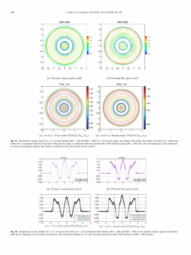
108 J. Zhai et al. / Computers and Fluids 134–135 (2016) 90–110
Fig. 17. The present counter lines of η = h + b with meshes 200 × 200 and 800 × 800 at t = 0 . 4 in the upper two frames. The lower two frames are from [16] , where the
lower left is computed with the first order PVM and the right is computed with the second-order PVM schemes using 200 × 200 cells. (For interpretation of the references
to colour in this figure legend, the reader is referred to the web version of this article.)
Fig. 18. Comparison of the profiles of η = h + b across the center at t = 0 . 4 computed with meshes 200 × 200 and 800 × 800 in the present results (upper two frames)
with those computed in [16] (lower two frames). The reference solution in [16] was obtained using first order PVM method on 800 × 800 meshes.
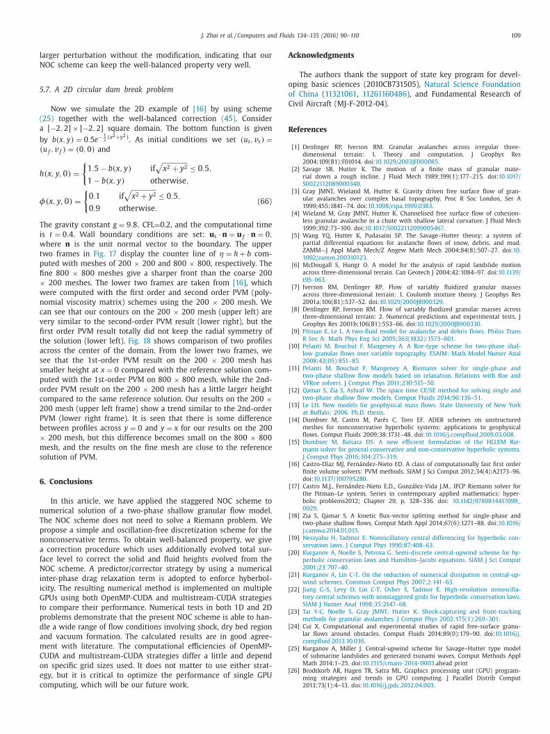
J. Zhai et al. / Computers and Fluids 134–135 (2016) 90–110 109
l
N
5
(
a
b
h
φ
T
i
w
t
p
fi
×
w
n
c
v
fi
t
a
s
s
p
o
c
2
P
b
×
m
s
6
n
T
p
n
a
f
N
i
i
G
t
p
d
a
m
C
o
e
c
A
o
o
C
R
[
[
[
[
[
[
arger perturbation without the modification, indicating that our
OC scheme can keep the well-balanced property very well.
.7. A 2D circular dam break problem
Now we simulate the 2D example of [16] by using scheme
25) together with the well-balanced correction (45) . Consider
[ −2 , 2] × [ −2 , 2] square domain. The bottom function is given
y b(x, y ) = 0 . 5 e −1 2 (x 2 + y 2 ) . As initial conditions we set (u s , v s ) =
(u f , v f ) = (0 , 0) and
(x, y, 0) =
{1 . 5 − b(x, y ) if
√
x 2 + y 2 ≤ 0 . 5 ,
1 − b(x, y ) otherwise ,
(x, y, 0) =
{0 . 1 if
√
x 2 + y 2 ≤ 0 . 5 ,
0 . 9 otherwise . (66)
he gravity constant g = 9 . 8 , CFL = 0.2, and the computational time
s t = 0 . 4 . Wall boundary conditions are set: u s · n = u f · n = 0 ,
here n is the unit normal vector to the boundary. The upper
wo frames in Fig. 17 display the counter line of η = h + b com-
uted with meshes of 200 × 200 and 800 × 800, respectively. The
ne 800 × 800 meshes give a sharper front than the coarse 200
200 meshes. The lower two frames are taken from [16] , which
ere computed with the first order and second order PVM (poly-
omial viscosity matrix) schemes using the 200 × 200 mesh. We
an see that our contours on the 200 × 200 mesh (upper left) are
ery similar to the second-order PVM result (lower right), but the
rst order PVM result totally did not keep the radial symmetry of
he solution (lower left). Fig. 18 shows comparison of two profiles
cross the center of the domain. From the lower two frames, we
ee that the 1st-order PVM result on the 200 × 200 mesh has
maller height at x = 0 compared with the reference solution com-
uted with the 1st-order PVM on 800 × 800 mesh, while the 2nd-
rder PVM result on the 200 × 200 mesh has a little larger height
ompared to the same reference solution. Our results on the 200 ×00 mesh (upper left frame) show a trend similar to the 2nd-order
VM (lower right frame). It is seen that there is some difference
etween profiles across y = 0 and y = x for our results on the 200
200 mesh, but this difference becomes small on the 800 × 800
esh, and the results on the fine mesh are close to the reference
olution of PVM.
. Conclusions
In this article, we have applied the staggered NOC scheme to
umerical solution of a two-phase shallow granular flow model.
he NOC scheme does not need to solve a Riemann problem. We
ropose a simple and oscillation-free discretization scheme for the
onconservative terms. To obtain well-balanced property, we give
correction procedure which uses additionally evolved total sur-
ace level to correct the solid and fluid heights evolved from the
OC scheme. A predictor/corrector strategy by using a numerical
nter-phase drag relaxation term is adopted to enforce hyberbol-
city. The resulting numerical method is implemented on multiple
PUs using both OpenMP-CUDA and multistream-CUDA strategies
o compare their performance. Numerical tests in both 1D and 2D
roblems demonstrate that the present NOC scheme is able to han-
le a wide range of flow conditions involving shock, dry bed region
nd vacuum formation. The calculated results are in good agree-
ent with literature. The computational efficiencies of OpenMP-
UDA and multistream-CUDA strategies differ a little and depend
n specific grid sizes used. It does not matter to use either strat-
gy, but it is critical to optimize the performance of single GPU
omputing, which will be our future work.
cknowledgments
The authors thank the support of state key program for devel-
ping basic sciences (2010CB731505), Natural Science Foundation
f China ( 11321061 , 11261160486 ), and Fundamental Research of
ivil Aircraft (MJ-F-2012-04).
eferences
[1] Denlinger RP, Iverson RM. Granular avalanches across irregular three-
dimensional terrain: 1. Theory and computation. J Geophys Res
2004;109(B1):F01014. doi: 10.1029/20 03JF0 0 0 085 . [2] Savage SB, Hutter K. The motion of a finite mass of granular mate-
rial down a rough incline. J Fluid Mech 1989;199(1):177–215. doi: 10.1017/S0 0221120890 0 0340 .
[3] Gray JMNT, Wieland M, Hutter K. Gravity driven free surface flow of gran-ular avalanches over complex basal topography. Proc R Soc London, Ser A
1999;455:1841–74. doi: 10.1098/rspa.1999.0383 .
[4] Wieland M, Gray JMNT, Hutter K. Channelised free surface flow of cohesion-less granular avalanche in a chute with shallow lateral curvature. J Fluid Mech
1999;392:73–100. doi: 10.1017/S0022112099005467 . [5] Wang YQ, Hutter K, Pudasaini SP. The Savage–Hutter theory: a system of
partial differential equations for avalanche flows of snow, debris, and mud.ZAMM—J Appl Math Mech/Z Angew Math Mech 2004;84(8):507–27. doi: 10.
10 02/zamm.20 0310123 .
[6] McDougall S, Hungr O. A model for the analysis of rapid landslide motionacross three-dimensional terrain. Can Geotech J 2004;42:1084–97. doi: 10.1139/
t95-063 . [7] Iverson RM, Denlinger RP. Flow of variably fluidized granular masses
across three-dimensional terrain: 1. Coulomb mixture theory. J Geophys Res2001a;106(B1):537–52. doi: 10.1029/2000JB900329 .
[8] Denlinger RP, Iverson RM. Flow of variably fluidized granular masses acrossthree-dimensional terrain: 2. Numerical predictions and experimental tests. J
Geophys Res 2001b;106(B1):553–66. doi: 10.1029/20 0 0JB90 0330 .
[9] Pitman E , Le L . A two-fluid model for avalanche and debris flows. Philos TransR Soc A: Math Phys Eng Sci 2005;363(1832):1573–601 .
[10] Pelanti M , Bouchut F , Mangeney A . A Roe-type scheme for two-phase shal-low granular flows over variable topography. ESAIM: Math Model Numer Anal
2008;42(05):851–85 . [11] Pelanti M , Bouchut F , Mangeney A . Riemann solver for single-phase and
two-phase shallow flow models based on relaxation. Relations with Roe and
VFRoe solvers. J Comput Phys 2011;230:515–50 . [12] Qamar S , Zia S , Ashraf W . The space time CE/SE method for solving single and
two-phase shallow flow models. Comput Fluids 2014;96:136–51 . [13] Le LH . New models for geophysical mass flows. State University of New York
at Buffalo; 2006. Ph.D. thesis . [14] Dumbser M, Castro M, Parés C, Toro EF. ADER schemes on unstructured
meshes for nonconservative hyperbolic systems: applications to geophysical
flows. Comput Fluids 2009;38:1731–48. doi: 10.1016/j.compfluid.20 09.03.0 08 . [15] Dumbser M , Balsara DS . A new efficient formulation of the HLLEM Rie-
mann solver for general conservative and non-conservative hyperbolic systems.J Comput Phys 2016;304:275–319 .
[16] Castro-Díaz MJ, Fernández-Nieto ED. A class of computationally fast first orderfinite volume solvers: PVM methods. SIAM J Sci Comput 2012;34(4):A2173–96.
doi: 10.1137/100795280 .
[17] Castro M.J., Fernández-Nieto E.D., González-Vida J.M.. IFCP Riemann solver forthe Pitman–Le system. Series in contemporary applied mathematics: hyper-
bolic problems2012; Chapter 29, p. 328–336. doi: 10.1142/9789814417099 _0029 .
[18] Zia S, Qamar S. A kinetic flux-vector splitting method for single-phase andtwo-phase shallow flows. Comput Math Appl 2014;67(6):1271–88. doi: 10.1016/
j.camwa.2014.01.015 .
[19] Nessyahu H , Tadmor E . Nonoscillatory central differencing for hyperbolic con-servation laws. J Comput Phys 1990;87:408–63 .
20] Kurganov A , Noelle S , Petrova G . Semi-discrete central-upwind scheme for hy-perbolic conservation laws and Hamilton–Jacobi equations. SIAM J Sci Comput
2001;23:707–40 . [21] Kurganov A , Lin C-T . On the reduction of numerical dissipation in central-up-
wind schemes. Commun Comput Phys 2007;2:141–63 .
22] Jiang G-S , Levy D , Lin C-T , Osher S , Tadmor E . High-resolution nonoscilla-tory central schemes with nonstaggered grids for hyperbolic conservation laws.
SIAM J Numer Anal 1998;35:2147–68 . 23] Tai Y-C , Noelle S , Gray JMNT , Hutter K . Shock-capturing and front-tracking
methods for granular avalanches. J Comput Phys 2002;175(1):269–301 . 24] Cui X. Computational and experimental studies of rapid free-surface granu-
lar flows around obstacles. Comput Fluids 2014;89(0):179–90. doi: 10.1016/j.compfluid.2013.10.036 .
25] Kurganov A, Miller J. Central-upwind scheme for Savage–Hutter type model
of submarine landslides and generated tsunami waves. Comput Methods ApplMath 2014:1–25. doi: 10.1515/cmam- 2014- 0 0 03 . ahead print
26] Brodtkorb AR, Hagen TR, Satra ML. Graphics processing unit (GPU) program-ming strategies and trends in GPU computing. J Parallel Distrib Comput
2013;73(1):4–13. doi: 10.1016/j.jpdc.2012.04.003 .

110 J. Zhai et al. / Computers and Fluids 134–135 (2016) 90–110
[
[27] Satra ML , Brodtkorb AR . Shallow water simulations on multiple GPUs. In:Jonasson K, editor. PARA 2010, Part II, LNCS 7134; 2012. p. 56–66 .
[28] Vinas M , Lobeiras J , Fraguela BB , Arenaz M , Amor M , Garcia JA , et al. A mul-ti-GPU shallow water simulation with transport of contaminants. Concurrency
Comput: Pract Exp 2013;25(8):1153–69 . [29] Bermúdez A , Vázquez-Cendóon ME . Upwind methods for hyperbolic conserva-
tion laws with source terms. Comput Fluids 1994;23:1049–71 . [30] Adusse E , Bochut F , Bristeau M , Klein R , Perthame B . A fast and stable well-bal-
anced scheme with hydrostatic reconstruction for shallow water flows. SIAM
J Sci Comput 2004;25:2050–65 . [31] Castro-Díaz MJ, Fernández-Nieto ED, Gonzáez-Vida JM, Parés-Madroñal C. Nu-
merical treatment of the loss of hyperbolicity of the two-layer shallow-watersystem. J Sci Comput 2011;48:16–40. doi: 10.1007/s10915-010- 9427- 5 .
[32] Tai Y-C . Dynamics of granular avalanches and their simulations with shock–capturing and front-tracking numerical schemes. Darmstadt University of Tech-
nology; 20 0 0. Ph.D. Thesis .
[33] Rogers B , Borthwick A , Taylor P . Mathematical balancing of flux gradient andsource terms prior to using Roe’s approximate Riemann solver. J Comput Phys
2003;192:422–51 .
[34] Zhang S , Chu YL . GPU high performance computing with CUDA. Chinese Hy-drology Publishing House; 2009 . [in Chinese]
[35] Sanders J , Kandrot E . CUDA by example: an introduction to general-purposeGPU programming. 1st. Addison-Wesley Professional; 2010 .
[36] Zhai J, Yuan L, Liu W, Zhang XT. Solving the Savage–Hutter equations for gran-ular avalanche flows with a second-order Godunov type method on GPU. Int J
Numer Methods Fluids 2015;77(7):381–99. doi: 10.1002/fld.3988 . [37] NVIDIA Corporation. NVIDIA CUDA C programming guide, version 6.0; 2014.
38] NVIDIA Corporation. CUDA API reference manual, version 4.2, 2012,
http://developer.download.nvidia.com/compute/DevZone/docs/html/C/doc/ CUDA _ Toolkit _ Reference _ Manual.pdf .
[39] LeVeque RJ . Balancing source terms and flux gradients in high-resolution Go-dunov methods: the quasi-steady wave-propagation algorithm. J Comput Phys
1998;146(1):346–65 . [40] Xing Y , Shu C-W . High order finite difference WENO schemes with the ex-
act conservation property for the shallow water equations. J Comput Phys
2005;208(1):206–27 .