'COMPUTERIZED SCHEDULE CONSTRUCTION FOR AN AIRLINE ...

'COMPUTERIZED SCHEDULECONSTRUCTION FOR AN AIRLINETRANSPORTATION SYSTEM

R. W. Simpson

FT- 66-3

ARCHIVES

MASSACHUSETTS INSTITUTE OF TECHNOLOGY

FLIGHT TRANSPORTATION LABORATORY

Technical Report FT-66-3

December 1966

Computerized Schedule Construction for an Airbus

Transportation System

R. W. Simpson

This work was performed under Contract C-136-66 for

the Office of High Speed Ground Transport, Department of

Commerce.

Computerized Schedule Construction for an

Airbus Transportation System

R. W. Simpson

December 1966

I.,

TABLE OF CONTENTS

Page

1 I. INTRODUCTION

7 II. DEMAND DATA GENERATION

15 III. PASSENGER FLOW PATTERNMethodology for Determination of F MatrixDescription of the Model for Passenger FlowInformation Available from the ModelThe Network Models for the VTOL Airbus SystemTypical Results

35 IV. DETERMINATION OF THE FREQUENCY PATTERN

41 V. TIMETABLE CONSTRUCTIONDetermining Suitable Departure TimesTimetable Construction Program

51 VI. OPTIMIZATION OF VEHICLE UTILIZATIONEnumerating Vehicles Required by a Given

TimetableA Logical Method for Reducing NF and WTA Statement of the Fleet Reduction AlgorithmResults of Application of the Algorithm to

Timetables

73 VII. RESULTING SCHEDULES AND DISCUSSION

89 Appendix A - An Extension of the Network Modelto Include Time of Day Demands

...... -' Wlffikiikll

I. INTRODUCTION

As part of a continuing study of the application of

V/STOL aircraft to the transportation problems of the

Northeast Corridor, the U.S. Department of Commerce has

requested that detailed data be developed on schedules,

travel times, and fares which might be expected for a

V/STOL system operating in the year 1980. This section

deals with the computer methods used to construct such

schedules.

A schedule (or more properly a schedule plan) is a

complete description of a transportation system. It de-

tails the services to be offered in the dimensions

of time and geography, gives the routings followed by

vehicles, and indicates the loadings to be placed upon

terminals. A complete statistical summary of the opera-

tion of the transportation system can be obtained once

the schedule is completed. The number of vehicles and

crews, their daily utilization, the expected load factors,

the required number of loading gates, the average length

of vehicle hop, etc. are all implicitly determined by the

schedule plan. Constructing and maintaining an efficient

schedule is the main problem of transportation system

-1-

.11

managements. It is both their production plan and their

product to be marketed, and the economic success of the

plan is gauged by the management's ability to produce a

low cost production which will be saleable to the travel-

ling public.

The use of computers in scheduling is not widespread

at this time, and if they are used, it is generally for

data processing as distinct from decision making or problem

solving. The reasons for this are clear. There has not

been in the past, sufficient capability either in the hard-

ware, or the software to handle problems of the size and

complexity associated with even such relatively small

transportation systems.as the airline systems. This situ-

ation has been changing in the last few years, to the point

where we can now begin to handle fairly large scale schedu-

ling problems, introducing optimization at several points,

and constructing fairly quickly and easily full systen

schedules and their statistical summaries. Parametric

investigations of the effects of restricting fleet size,

terminal size, etc. can be quickly carried out. Various

strategies or policy decisions are similarly easily inves-

tigated.

-2-

The construction of computer programs for the schedu-

ling process immediately points out the need for detailed

accurate data concerning demand. This is now becoming

available to the airlines through their reservation sys-

tems and the management information systems evolving from

them. We need to know, for example, detailed information

on the number of people travelling from A to B throughout

the day, by day of week and month of year, with an accuracy

much greater than our present estimates. We would like to

know the demand elasticity, e.g. the change in the number

of people travelling as services are changed in time or

quality for every service pair in the system. The charac-

ter of the available data (as distinct from opinion) deter-

mines the type of problem that operations research and the

computer will be able to successfully solve. Various large

scale econometric models are conceivable, if revenue and

cost data are available.

This section will describe the work which has been

carried out for a hypothetical Airbus short haul V/STOL

system in the Northeast Corridor. It is only a beginning

as valuable extensions are yet to come as more applications

-3-

come into the open literature. The main presentation

will describe the computerized processes developed to

construct a schedule plan assuming certain demand and

operating data. An interesting extension showing the

application of network flow theory to a more detailed

representation of the schedule is then described in

Appendix A.

A map of the corridor showing the terminals selected

for the Airbus system is shown in Figure 1. Table I shows

some typical distances, travel times, and projected fares

for the 1980 Airbus.

-4-

TABLE I

Typical Fares and Travel Times

VTOL Airbus System

TRIP

Washington downtown

- Dulles

- Baltimore downtown

- Philadelphia downtown

- New York downtown

- Norfolk

- Providence

Distance

(st. miles)

26

33

123

203

144

351

Time

(minutes)

6

7

22

34

25

58

Fare

(1966 dollars)

3.10

3.35

6.55

9.35

7.25

14.60

Boston downtown

- Worcester

- Providence

- Hartford

- Laguardia

- Philadelphia downtown

- New York downtown

From

to

From

to 40

46

89

181

266

190

8

9

16

31

44

32

3.60

3.80

5.35

8.60

11.60

8.90

-5-

0 30 60miles MANe

FITe

eWBA

AMEWI

ALL*

REA*

ISP-EQU

LGA

STUDY AREANORTHEAST CORRIDOR

TRANSPORTATION PROJECTUNITED STATES

DEPARTMENT OF COMMERCE

* MAJOR TERMINALS' SMALL TERMINALS

VTOL AIRBUS TRANSPORTATION SYSTEM

FIG. I

-6-

HARe,\

YRK. eLAN

14 /p

II. DEMAND DATA GENERATION

The methods of generating demand data have previously

been described in Reference 3. A brief description of

these methods will be given here along with some detailed

description of the data for a second demand assumption.

The computerized methods of timetable construction of

this report assume the availability of explicit , detailed

information about the passenger demand for services between

any two system points. Accordingly, a method of generating

such data was developed using a modified "gravity" model.

The model uses projected 1980 populations for each system

point (see Table 2), and the distance between points to cal-

culate the number of passengers per day between each pair of

points.

The model has the form:

dij = K -[ ' x l - e S ASIJ I

where K is a scaling constant; and the first bracket is the

gravity model with Sk = 0.4. The second bracket represents

a modification to represent the share of air travel in compe-

tition with the automobile, bus, and train, etc. The constant

-7-

lmolkilli,hl 4 IIIIIIIIi a rsl1-1m r -10 - 1 -1 ,m i

TABLE 2. NORTHEAST CORRIDOR AIRBUS TERMINALS,

POPULATIONS, AND OPERATIONS PER DAY

Terminal LocationsCodeDesig-nation

1980Population

PassengerOrignations

Per Day

AircraftOperations

Per Day

MAJOR TERMINALS

Boston, Mass.-LoganBoston, Mass.-in or

near downtownNew York, NY - John

F. Kennedy Internat'lNew York, NY - La-

Guardia AirportNew York,NY - Wall

Street HeliportNew York,NY - Pan

American Bldg.Newark, NJ - Newark

AirportPhiladelphia, Pa. -Philadelphia AirportPhiladelphia, Pa. -downtown on the riverBaltimore, MD - Friend-

ship AirportBaltimore, Md - in or

near downtownWashington, DC -Wash. Natnl AirportWashington, DC -

downtown

OTHER TERMINALS

Portland, Me. -Portland Airport

Manchester, NH -Gernier Airport

Lawrence-Haverill,Mass.Lawrence Airport

Fitchburg,Mass. -Fitchburg Airport

Pittsfield, Mass. -Pittsfield Airport

Worcester, Mass. -Worcester Airport

Brockton, Mass.-Brockton Airport

Providence, R.I. -Providence Airport

New Bedford, Mass.-New Bedford Airport

BOS

BOC

JFK

LGA

JRB

NYCEWR

PHL

PPABAL

BMR

DCA

WAS

1,478,500

1,508,800

2,818,800

3,801,600

1,097,000

1,701,7001,933,800

2,413,900

3,653,100757,700

1,850,900

1,162,00

1,801,956

3770

2830

4252

5641

1632

25322942

4537

67601458

3591

2211

3430

249

218

377

197

.203

734

445

1891

168

154

240

798

126

272204

298

646601

300

112

244

104

PWM

MAN

LAW

FIT

PIT

WOR

BTN

PVD

NBD

136,000

111,700

198,400

100,000

90,800

368,100

232,900

941,500

146,100 193

-8-

TABLE 2. CONTINUED

Terminal LocationsCodeDesig-nation

1980Population

PassengerOriginations

Per Day

AircraftOperations

Per Day

Reading, Pa. -Reading Airport

Harrisburg, Pa. -Harrisburg Airport

Lancaster, Pa. -Lancaster Airport

York, Pa. - York Air-

portTrenton, NJ - Trenton

AirportAtlantic City, NJ -

REA

HAR

LAN

YRK

TRE

Atlantic City Airport ACYWilmington, Del. -

Wilmington Airport WILWashington, DC - Dulles

Airport DULRichmond, Va. -

R. E. Byrd Flying Field RICNewport News - Hampton

VA - Civil Airport PHF

Norfolk, Va. - NorfolkAirport ORF

Springfield, Mass.-Springfield Airport

Hartford, Conn. -Rentschler Airport

Hartford-Springfield -Bradley Field

Waterbury, Conn. -Waterbury Airport

New London, Conn -New London Airport

New Haven, Conn. -New Haven Airport

Bridgeport, Conn. -Bridgeport Airport

Norwalk, Conn. - SW

of downtown near water

Stamford-Greenwich,Conn.-Between Stamford

& Greenwich near wat.

New York, NY - Teter-

boro AirportLong Island, NY -Mitchell AFB(abandoned)

Islip, Long Island,NY - MacArthur Field

East Quogue, Long Is.NY- Suffolk Cty AFB

East Hampton, Long Is.NY - Airport

Scranton, Pa.-ScrantonAirport

Wilkes-Barre, Pa. -Wilkes-Barre Airport

Allentown, Pa. - Allen-

town Airport

SPR

HFD

BDL

WBY

GON

HVN

BDR

NWK

SGC

TBO

MIT

ISP

EQU

EHM

AVP

WBA

ALL

667

1037

814

132

108

694

635

509

319,500

431,300

391,900

329,900

357,900

239,600

631,200

776,900

633,000

570,500

972,500

636,100

693,700

182,000

250,300

254,700

416,600

499,600

196,800

796,200

1,023,200

1,627,200

417,700

292,200

1337

1501

1246

1107

1868

168

140

1336

1431

380

506

535

804

908

331

1301

1555

2508

741

628

266

403

634

1259

216

126,100

194,200

271,900

621,700

-9-

nation

C is chosen such as to cause a specific peaking of the d

variation with distance (e.g. for 200 miles C = .007, for

100 miles, C = .015). The value of is taken as 2.0.

This data is not a prediction - it is a hypothetical

pattern of demand generated to examine in detail the problems

of producing a schedule or timetable by computer, and to

allow some idea of desirable vehicle sizes, terminal sizes,

number of operations, vehicle and terminal utilizations, etc.

to be obtained. Both the scale and the pattern of demand

can be changed in order to examine the sensitivity to such

changes of certain operational information arising from the

system schedule. It is expected that detailed projections

of Northeast Corridor demands from other Department of Com-

merce studies will become available at some future date. As

a result of the studies reported in Reference 3, a second

pattern of demand has been generated with the peak of the pat-

tern shifted from 200 to 100 miles. See Figure 2. Such a

shift assumes that the air system will have a larger share

of the total travel market, particularly for trips below 200

miles. Since the previous results indicated appreciable time

savings, and lower costs, this shift in demand was indicated

in generating a second demand pattern.

-10-

50

40

DEMND MODEL 2

30

L CL

F-J20 _ C0.007 DEMAND MODEL 1

10 - D -3xlO -7 x e- (Cd) 2

P P2 d 0.4

0 1 1 1 110 100 200 300 0

DISTANCE ,d, (Statute miles)

N.E. CORRIDOR DEMAND FUNCTION FOR AIRBUS TRAVELFIGURE 2 ASSUMED

The demand data is given in Table 3. It is a 50 x 50

matrix called the D2 matrix, with a subscript 2 to indicate

the second demand pattern. The data is 0 & D data (origina-

tion and destination) where the matrix entry dij gives the

number of trips per day from point i to point j. As is

generally true for passenger traffic (but not cargo or

freight), the matrix of Table 3 is symmetric, where di =

d . The diagonal consists of zeroes, and the sum of any

row represents the number of trips out of a given point, i.

Similarly the sum of any column represents the number of

trips ending at a point j. Table 2 gives the number of

passenger originations for each station for the D2 matrix.

The second demand generates 27.7 x 106 passengers per year

compared to 16.7 x 106 for the first demand matrix, D1.

Each entry, dijs represents a best estimate of the mean or

average of daily travel demands on the system over some period

such as a peak month or season. Daily demand varies from day

to day in recognized seasonal and weekly cyclic patterns,

and is a probabilistic or stochastic variable. In this study,

dig represents the mean of such variations over all days of a

peak month or season, and a system load factor is assumed

later to be 60% to ensure that daily demands above the average

-12-

TABLE 3 - DAILY TRIPS BETWEEN CITY PAIRS - SECOND DEMAND

J ci 02 00 < z j C 4 M j a 4 mj w Z m- X0>- 2 L F Co IL cc If 0 0 x uk u x 2a3U D 4 0 0 4 0 > - I 2 M 4 ._j < 0 a. - 0 t 0 2 3 a y 1 o I 0 2 < - t 2 - x. 4 w > n ; 0 x -c o co I ca > z a. 3 a I F r a r 3 0 a o , 0 - w m I 3 v x < I 3 3 1- 2 0 2 a a. 4 o 2 - ww a- - J

DCA 691ii i 5T T i 88 329 47 43 5o 8 T 6 34 64 9 1813331449 131235 54 44 26 26 11i 32 95- I9 22 203 131 1 e 497 78 38 2419{_C 56197 2934 221

5 *[16 30 13 1 21

DUt 32 o 92 712319160o69 i 9 34 L 85 42% 36 61 I7I 2i9 f1 47| 21 94H 37 92315" 13236 255 32 912 25 16 59 4 3 9 8 6 2

-AL 2 9 i 4 81 32 26 26 55 33431I 7 412 6 4 6, 31, 50 18 6 32 9 8 6 5 21 1 j 920 309 91 242 37 6344 17 48 213 0 7~ -1 30 1 140-_ _ - -1 F5121os7N 1 is 1 so if 6 89 29 4 46 ,603 17i 290 86 721 43; 40 3 1226 2 161 268,107 69 6 27'33 33. I 22 7

80C 9 1 191 35 52 44 52 962! 3 9j95 1 29 459 621 17 307 88 73, 44 40 111 3 27 2 i750" 513! 6442269 i1 2 1 22 23 6 7

MAN 24 3 7 5 0 3 ' 1 9 23710 6 53 12 ~~3MA2i aI f 31 1f-3 - 5-331 1 55170i1431722718- 2-WOR 4 I 18-3-, 62I3 16 01 1 1 21 16 9 8 1 9 5 5 72 27 18 132 1 6 7 3 8 2 5 6 101 55

N80 9 6 1 3 4 3I o33; S5 3 3 ii I i 9 24 7 127 1 6 l4e 12 1 s 5WVL 224 30 87 1 5 8 6 1 4 2 1 i 7 7_ v - 4 60 2221 35293 594 12 49IO 1 0 7 1 1 52 40! -7 148i1 2!95I 3 I0I I3i hiw 387tI4-22 s2 2' I6 i -5 I9 IWIL 7 IV I4i 4 3if529 6il 24 53 6 32 2 2

TR E7 7 4 4 6

REA T 1 7 4 7 900 8414 0 69 1 8 3 67 61 61 3 230 , 43 9 2 7LAN 24 2 I9 0 21 Sl 1 2 7L 1 2 4 7 2 ,2 48 30, 8 12 5 4 4 18 7

R 4 Idi s -- 2 i e1 8 4 s i_ 8

WBA 9 I I 6 ~5 4I I9 18 5 52 15 5 6 6 3256 6 4 5 0 7 1 6 fSPR I I i4 4i li

ti Ii ii 2 s 12e 29 6l [2i2- 0 e- 1 4 3

- - 12 1 1i 040 12 2 i 5 4 -

eDL ] Is'l ie 3 7 3 475 4 7

JFK: 6 So 8 9 2 1i-6 4c4 1 So 6 -4 - -

-4- 1 -- - 1 291 - 36_1- f _

JR0 23 6 15 38 30 2 9 414 923N I 2 60 61 2 9 80 1211 3 57013 278 81 5 2 6 324 11 28 46 910 2i 86i363 5 1

WBy 4 62 I 5332 1 e 6472 5 ' 4 7361N 91 of 3 5 4 9 12 7 1 6 216 8 1 5 1 6 3 4

HFD 32 2050 2 14 28 50 2 9 1 0,9 11'7 2,4 2 2:2 9 1 4 13 29 70 7 0 1 6 !

4 1 -f I j0 Ii ! 1f I-~ I i R 7-2 - 2T01 8 214

ACY5 6 41! 3 457 2 102? 3 1 1 T1 2 2BMR1 59 48 23 41 7 t 15 31 3 1211 9 1 8641 4017 3 49 5 9 3 34 4

wFs r08 ii 6 s0 as' h r 4

522R 1 52 5 134 7 1102146.273 62 4 71 li 3, 3241 72i 39

TBO 1 T 12 8 2 2231

-69N 02 f8 2 21 331 12 457' 195 19 84 5 6 5 476 4 9

R 3 [ 3 6 21 252 69 2 1 1 3 1 24 7 1541112EW i 7-_1 58 Ii 1- 3i- i l-il-7 11 65 10 5 41 71 22 1 1 I28 24'- 21 4- 3

WRY 2 4 9 2 4 2-1 5 41 3 24 1 41 2 9 13' 2 I 2 3 15I 7 6 1 1

PPA 5o 64 149 3 35626

- I I -ii tT 16 - 9 3i 7 I -i 4--

WY 44j s1 1 9 7 I3 40 45 1 3 0323 018 20 937.7301 129.94 8 4 0 5 9 3WAS 1 I4 35I 22759 32 22 15 4,,

18 19 Il 119 79Tl f l j 13---I-I W ~ 11 i 11 31281

MC 9 5 4 1 ,2 13 2

NW 24 5-2-

III I I23.2- 1 08 149 93 7,3 81 1 61 84 -7 78I49 29 8 2 3

NYC Iil2- 121: 71 12 56 -8 4 1 4 73 i4.-i.IiI C9R4,-i

NRYCI1 - 1948197 16244 88j 6313714 i 425, ii i3OR I I I Ii I4 10 357 I~ j~ 17 14' I

RIC 681 24 11 441 ' I 41141215 621 9 43 1359P M I 2 4PHI' I 20 1040 10 129 14 6 5 4 10 8

YRK -t 14 I iI- 84 9 99 49 3 580 665

SGC 1 10 22 9 ' '

NWK r 2 5 2 3 - 5 90 129 49

II I HtI I~ 1~ 3-4519F IT 2BTN T

LAWF J V 0 Z : I Z I I q _: In , , o- o w n <Q mLA - 1 11 1 1 0 I j4 . 0 v It 1, 1 > L a- X

> ' 01 f LJ 1I KL .9 1 J1In m ml X 2n 2 j 0 .o 4 LU m~ A -2 10 a In._

are accommodated. Variations of demand with time of day

are accounted for by choosing departure times in the time-

table construction.

The demand data assumed available here is similar to

that obtained by the CAB in its present method of sampling

ticket sales and recording the 0 & D flow by all airlines

between various points. If the airbus system were operating

with a computerized reservation system or more precisely a

management information system, such data could be continuously

gathered and made available for any time period. Future pro--

jections could then be based on this data in planning sche-

dules for future time periods.

Often, a more detailed description of demand can be

available for purposes of schedule planning. For example, the

weekly cycle of demand could be studied with the goal of

providing different daily timetables, or a semi-weekly schedule;

or, competitive factors between companies or between modes

could be available. No such complexities have been allowed

here. The abject has been to provide some idea of the geo-

graphic distribution of daily demands in order to determine

the frequency of service pattern for the assumed system. This

process will be described in the next two sections.

-14-

MMW M011111111

III. PASSENGER FLOW PATTERN

The demand matrix, D, gives the number of trips per

day from City A to City B. Unless the system is providing

direct non-stop service between all city pairs this will

not be the totality of passengers using the route A-B since

other "through" passengers will use the route in going

X - A - B - Y. For 50 cities there are 2450 possible

non-stop services, but not all of them will generate suf-

ficient demand to warrant non-stop service. This can be

seen by examining the D matrix. On most airline systems2

only about 15-20% of such possibilities are economically

attractive, so that there is a substantial percentage of

through passengers on most direct services.

It is necessary to have some method of determining the

passenger flow patterns for a given subset of non-stop

services. The total passenger flow (non-stop plus through

passengers) then determines the daily number of non-stop

seats required, or the frequency of daily non-stop service

required for a given vehicle seat size and load factor.

This process is sometimes called detennining the frequency

of service pattern for the system. Lesser routes are dropped

-15-

-- a I k I I I I, I I I I I I I , j .

to zero frequency in favor of higher frequencies else-

where.

This section will describe the techniques used to

produce a passenger flow pattern (the F matrix) given the

subset of routes to be serviced. We are interested in

matching available seats/day against passengers/day on

each route to be serviced in order to obtain the frequency

pattern (the N matrix)in the next section. In other words,

we are trying to determine on a system wide basis a balanced

allocation of available seats to the geographic patterns

of demand.

A multi-commodity network flow computation is used

to re-route the passengers from X to Y via the shortest

routing X - A - B - Y. Initially, an assumption has been

made that least distance can be used as a criterion for

determining the "shortest" routing. It is probably a good

representation of least time when the frequency of service

on all routes is fairly high, and the model can be exten-

ded (as shown in Appendix A ) to be precisely least time

when the time of day network and a discrete timetable are

used. It is assumed that a passenger will use the services

which have the earliest arrival at Y, and that the indirect

routings will not have an effect on the D matrix demands.

-16-

M11111111011MOMMIM110111111 III, 111 1111

Neither of these assumptions can be rigorously defended.

In the airbus system, it is planned that knowledge of the

earliest available arrival at his destination via indirect

routings will be available to the passenger through the

system's computer, and that intermediate stops will delay

the flight only a few minutes. Both of these factors will

tend to make the assumptions more applicable to airbus ser-

vice than to present airline service.

-17-

1.1

Methodology for Determination of F Matrix

The methods used to determine shortest paths and

the passenger F matrix are drawn from network flow

theory, and the theory of graphs. A fuller theoreti-

cal understanding of these concepts can be obtained

by reading Reference 4, and then Reference 5. A brief

explanation of the techniques will be given here.

The computer program .sed was a modification of

an IBM SHARE library coding by Dick Clasen at Rand

Corporation for the "Out of Kilter" OKF algorithm of

Ford and Fulkerson. This algorithm is applicable to

large transportation network problems where the num-

ber of arcs and nodes can be 4500, and 1500 respect-

ively. Solutions give integer values of xij and are

obtained within 10 minutes of computation on an IBM

7094.

Suppose we have a network or graph G which con-

sists of nodes (i,j,k...) and directed arcs (ij, jk,...)

such that closed paths or circuits exist in the graph.

With each arc ij, there are three associated scalar

quantities;lii = lower limit on arc flow

uij = upper limit of arc flow = capacity

cii = unit cost of flow from i to j

-18-

MIMTFI I

and the variable x.. which is called the flow of some com-1J

modity from node i to node j.

We wish to determine a flow X = x.., X. ,... such

that:

1) 1.. ( x. u.. Capacity constraints1J 1J 13J for all arcs.

2) (x.. - x ) =0 Conservation of flow

(i., jk) at nodes j.

3) x.. are integer values1J

and which will minimize the total flow cost,

Z =c.. .x..

arcs ij

This is recognizable as a special case of the general

linear program where a.. =0, + 1, and is called the transpor-1J

tation or assignment problem. It is widely applicable to a

variety of transportation or scheduling processes, particu-

larly since the size of the Out of Kilter algorithm and its

integer solutions allow practical problems to be solved. If

posed as a linear program, there would be 4500 variables with

9000arc equations for the upper and lower constraints and 1500

node equations.(i.e.a'matrix of 10500 rows and 4500 columns).

Since most of the a.. matrix entries are zeroes ( matrix den-1J

-19~

MINIM1111"u.111i NAH M111IM11 IN NEW ,

sities for this type of problem are typically 10 percent), the

labelling technique used by Ford and Fulkerson is far more

efficient than any variant of the Simplex technique. If l..1J

and u.. are integers, we are assured that any feasible solution1J

for X will also be integer.

-20-

lop 19 Il III I 1111IT11 101 1111111 IF jill 1191

Description of the Model for Passenger Flow

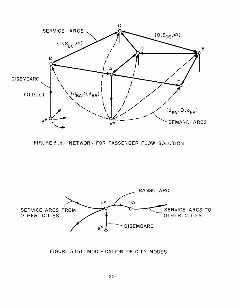
To use this technique, it is necessary to construct

a graph or network as a model or representation of the pas-

senger flow problem. Figure 3 shows a simplified network

representation of the model.

The subgraph of "city" nodes A, B, Ce.. and

"service" arcs [AB, BA, AD, DA, ... represents the geo-

graphic or service network of cities A, B, etc. and

non-stop services operated between cities AB, BA, etc.

If service between cities A and B is to be operated non-stop,

then a pair of directed "service arcs" AB and BA exist in

the service network. In Figure 3 this pair of arcs is repre-

sented as a solid line with both directions indicated by

arrows. Each arc has its cost (cij) value set to s, the

distance in miles between the city pair. Every service arc

has lii = 0, and u = 00 . Thus, there are no capacity con-

straints on the flow in service arcs, and the value of the

flow, xij, will represent the number of passengers/day wishing

to use this service.

The arcs LAA*, BB*, etc. are another subset of arcs

called "disembarcs". Nodes [A*, B*, C*,... are called

-21-

SERVICE ARCS

(0S Bc

B

( 0 ,SCE' O)

DISEMBARCN,

(0,D,co) (dBAOdBA)

tI (d 0O d)

~ DEMAND A

FIRURE3(a) NETWORK FOR PASSENGER FLOW SOLUTION

TRANSIT ARC

IA

SERVICE ARCS FROMOTHER CITIES

FIGURE 3 (b)

SERVICE ARCS TOOTHER CITIES

DISEMBARC

MODIFICATION OF CITY NODES

-22-

RCS

station nodes. There is one disembarc for each city. Their

values of lii and u are 0 and 00 respectively as for the

service arcs, and the cost for these arcs is D, the diameter

of the service network. A diameter is the longest track or

elementary path in a network, and this value is placed upon

these arcs to prevent flows from disembarking at an inter-

mediate station and travelling via demand arcs to their des-

tinations. The value of the flow in a disembarc represents

the number of people arriving at that station per day. It

will equal the sum of the associated column of the D matrix.

From every station node [A*, B*, C*, ... ] there isa subset of arcs called "demand" arcs. For example, from

node A*, a demand arc exists going to all city nodes [ B, C,

D, ... ] . The cost on these arcs is zero, and both lii and

uig are set to a value representing the daily demand in pas-

sengers/day between city B and all other cities. These demand

arcs ensure that a flow x.. equal to the demand d exists in

the demand arc, and necessitates a return flow via the shortest

path through the service network. For example, the demand

arc A*E in Figure 3 causes a flow in the service network back

to A and A* via either EDA or EFA whichever is shortest. The

node conservation constraints cause all flows in the complete

-23-

11011"

graph to be circulations, or flows in a circuit. For an

n-city problem, there will be n x n-1 demand arcs. If the

demand is symmetrical, some modifications can be made to

avoid repetition of demands. In this case, there are only

n x n-l demand arcs.2

At this point, the multi-commodity aspect of the problem

is encountered. Every x.. flow into a given city must be

considered as one commodity, xig, to prevent the flow x

along the shortest path in the service network from being

exactly cancelled by the symmetrical flow, xji, along the

identical path in reverse order. A modification of the

labelling technique in OKF was made to remove the reverse

labelling. In this way, an x.. value, once placed in the

network, could not be removed, and the return flow, x ,

uses the symmetrical forward path along the other member of

the service arc pair.

Since there are no capacity constraints on service arcs

in this problem, the multi-commodity aspect can be handled

efficiently within one run of the OKF code by solving for

each city sequentially. The "Alter" option of the coding was

used to impress new demands for the flow into the next city.

-24-

The complete solution for a 50 city case takes around 10

minutes on the MIT IBM 7094 while in CTSS operation. (Com-

patible Time Sharing System).

-25-

01%

Information Available from the Model

This modified algorithmic process will minimize the

total flow costs over the complete graph:

i.e. Minimize Z = c.. x s. x + x DJIJ 13 ij i ijiservice

arcs disembarcs

But, since D = constant, and for any given demand the xij in

the disembarcs is fixed equal to the column sums in the D

matrix, i.e., the total number of originating passengers per

day, P.

Min (Z) = Min s. x + P.D

service 3 i]arcs

= PM. + P.Dm.in

The constant RD is readily calculated and subtracted from

Z to get PM min. We are minimizing total passenger miles (PM)

in the network, and every individual passenger will be travel-

ling his shortest route since there are no arc capacity con-

straints.

The average passenger trip distance is then:

PM

p PV

-26-

I -

By a simple trick of splitting the nodes A,B,C...L

into two parts separated by a "transit" arc, as indicated

in Figure 3b, further information can be obtained. For

example, node A becomes two nodes: IA which receives all

service arcs from other cities, and OA which starts all

service arcs out of city A. The transit arc IA, OA}

has a flow which is the number of people passing through

the station on their trips to other destinations.

The number of passenger departures per day, PD, is

obtained by summing xi in the transit arcs and adding P.

PD = x + P

transitarcs

From this we can obtain the average hop or non-stop

distance for both passengers and vehicles:

-~ PMD = -H PD

-27-

As well, the frequency distribution of hops can be

obtained. If we categorize service arc distances, then

the sum of x.. for arcs in each category are an indica-1J

tor of frequency.

The average number of hops/passenger is

-- PD

P

The most detailed information available from each

solution is X itself. For the service network X = (x.

for all ij in network), is precisely the F matrix which

gives the number of passengers/day using each service.

It is possible to obtain the indirect routings and

the number of passengers per day on them. This has not

been carried out as yet. That information could be useful

in constructing flights consisting of a series of flight

segments by the same vehicle at a later stage in the

schedule construction process.

-28-

The Network Models for the VTOL Airbus System

For a system serving the 50 shopping points shown in

Figure 1, a model was constructed. There are 2450 possible

demand arcs which obtain d.. from the demand generation1J

program. There are 50 disembarcs, and 50 transit arcs,

and somewhere between 200-500 service arcs. The distance

costs, sig, are the great circle or airline distances used

in the demand program. The value of D was set at 1000 miles.

Several solutions were obtained for both D and D2

demand matrices, using different service networks. The

service networks were selected on two criteria. The first

was geographic where each station was connected to two of

its closest neighbors by "basic" arcs. These basic arcs

were members of every service network.

The second criterion was either demand, d.., or pas-1J

senger flow, Xi Table 4 describes the sequence of runs

for the second demand, and indicates how the various service

networks were selected. A strategy of including arcs of

lesser 0 and D demand dii was followed in the first four runs,

and the frequency of service pattern determined as explained

in the next section. Adding more and more non-stop services

dilutes the service to the point where a small number of

-29-

Mi,

TABL 4. COMUTE RUS FO SEONDDEN~flDATA

Description of ServiceNetwork

DH

Average Hopiailes

Total Pax-milesper dayv

No. ofService

Arcs ~

PDNo. of DailyPax. Depar-

tuires

Basic network - two

closest stations

2 Basic, + all arcs whered. > ..,300 pax./day

3 Basic, + all arcs whered > 200 pax./day

4 Basic, + all arcs wheredi j, 100 pax./day

5 Run 4, minus non-basicarcs whose xij 4 100

6 Run 5, minus non-basicwhose xij ( 150

7 Run 6, minus non-basicwhose xij ( 250

58.4

74.7

11.47 x 106

11.32 x 10

11.19 x 106

87 ,4

83.3

79.1

11. 22 x 10 6

11.25 x 10

11.28 x 10

Run

48.5 208

250 196, 371

332 151,414

534

410 128, 249

360 135,134

316 142, 454

TABLE 4.

n r d y Ar s

COMPUTER RUNS FOR SECOND DEMANDDATA

passengers per day were using various lesser services. The

strategy then became that of dropping service on these low

density routes and asking these passengers to proceed in-

directly via routes which enjoyed higher passenger flows.

Basic service arcs were always retained so that no station

could be isolated. Passenger flows on basic arcs is often

very low, and can be used to consider dropping the station

from the system.

-31-

TABLE 5 - THE PASSENGER FLOW MATRIX (F) AND THE FREQUENCY PATTERN MATRIX (N)

SECOND DEMAND, RUN 7

00W 01o e 2 2 a W

OCA 126

SALSOS 1087 LSOC 4 141 2 5MAN F1l 4WOR 5NBO 278

P t 3 ~PHI L 14TREREA

WA L 1SPR 6PITSDL -T

JFK 7 7 6 7LGA 8 12 24 9 16 9

E WR 15 9

HVN

WBYGON 6 11 6HFO - 7 6 21A C YIBMR 12 7

WAS 8 I ij

NYC 2

ORFRIC 7PPA 4 17 15 12 7 1PHF 1YRKAVP

ISPEQU

EHMPWMF IT1 4 8BTN 2 9LAW 14 L

F MATRIXx m w1 4 4 Wa. I- 4

56690

1703 159 288I899

63 I

10

1 63

7

24 5

8

14 1 -J 0 () .7 a 0 0J 4i 1*3Io :* 40 04 0 0>'i aa0a1w0 0 W z 3 2 ( I.l-

16

2

1-

8 7 5-,

6

t7

7

!a a-4 4 0 a) w. z

659766436

700 1135594 232 830 L

530 18601

62711533

968 1798 614538 219

.62?755

751 751 t638 684

66 585 1531463

6959 182 602

16 20 1796 1374 2012 86 878

7 9

4 1 970 - 12 851

9 7

12 14 7 16 27

6 _19 8_6 1 10110 14

3 32 4 1410

5

10 16 29 18 11

7

6

a i , J~ 4W 0m Z>

DAILY PASSENGERS- BOTH WAYS1 0 >- m (n 2- 0 0 IL >4 LWx a u . 0. I z0 IL 23 4 - W M- M r 0. X~ > 0 .> 0 an I ': 1: 1- 40 m 4W . W 1- 0 m a 0>1 4 0 z - d us mi IL 04

17991]752

1181 2801667583 j827j

183-587 78 1172

633

k I881570 522 9731

1012 1345 1886 983 1331617

646 715 960

572 15951-61

16641 509

6-.

6 6 6

8

-8 9 -5 14 15 17 1

4

<F

T Liisj

7-I---1-1

620 14

f1687.f 11144

2D64 lt607 f

8 9 9 37 3 f_ 7 2 5 -24

692

936

259 148415195172942 6 i120 340 7141307 102$

L

805401763 514 7451138C

733 503 1142

54 63

763

261

171-]I--

I -k-.1-.

2093 867 8242957

--70

1094 616

9 0 12 850 758 5751

9

2886 16727

2 LI I ii r44*o . W I

DAILY FREQUENCY - ONE WAY

65 1121399 49

75

854

39

18

m--

N MAT RIX

Typical Results

Results from the final run for the second demand are

given in detail in Table 5. Entries in the upper half of

the matrix are xi= passengers per day using service ij.

Other interesting results are given below

Total pax-miles/day = Z = 11.28 x 106

Total Passenger Trips/day = P = 76000

Total number of Passenger Departures = PD = 142,454

Average Passenger Trip Distance = Dp = 148.5 miles

Average Hop Distance = DH = 79.1 miles

Average No. of Hops/Passenger = 1.91

The distribution of hop distances is shown in Figure 4,

compared to the distribution of city pair distances for the

50 stopping points.

-33-

iflu

100-NORTHEAST CORRIDOR

50 100INTERCITY AIR

200 300 400DISTANCE -N. MILES

DISTRIBUTION OF INTERCITY DISTANCES (ALL CITY PAIRS)

50 100 200 300 400VEHICLE HOP DISTANCE - N. MILES

DISTRIBUTION OF VEHICLE FLIGHT HOPS

FIG. 4

-34-

80

60h-

40[-

VTOL AIR SYSTEM

T20

0

FIG. 4 (a)

a.0

z O00

QWa3-

zOL0

FIG.4 (b)

IV. DETERMINATION OF THE FREQUENCY PATTERN

Given the expected number of passengers/day using

a given route, an estimate of the desirable number of ser-

vices or direct flights/day can be obtained using vehicle

seat size and an average load factor established by plan-

ning policy. If we let N be the number of flights/day;

N. Xj=ij

< S . LF

where x = daily passengers from i to j - one way

S = vehicle seat size

LF = desired average load factor

< > signifies rounding off to next highestinteger.

At the present time, it has been assumed that there

is only one vehicle size (80 passengers), and that for planning

purposes an average system load factor which should be

achievable is 60%. Other combinations of vehicle size

should be studied since within the present models there

are indications that a smaller vehicle on the low density

routes should be used to increase daily frequencies of service.

The average load factor of 60% is chosen to allow for

monthly and weekly cycles of demand, and to account for the

-35-

fact that daily demand is a probabilistic variate from day

to day. When a fixed seating capacity is matched against

the average of a probabilistic quantity, a capacity margin

above the average load is required to ensure that the above

average loads can be carried.

The time of day cyclic variations can be accounted for

in two ways: allowing load factors to vary with time of

day, and by bunching departure times at the peak hours.

Both methods are discussed in the next section.

It is assumed that a daily schedule will be established

for the period of the demand estimate. If more detailed

information were available regarding weekly variations in

demand, considerations could be given to such things as a

semi-weekly schedule or special schedules for Saturday, etc.

Typical cycles of demand are shown in Figure 5. Similar in-

formation can be generated and estimated by the management

information system for the Airbus system.

It has also been assumed that there is no information

on competitive or marketing considerations which would dif-

ferentiate one route from another. Normal domestic airline

competition causes frequencies to be added by competing air-

lines to the point where marginal revenues tend to equal

marginal costs. As such, a variation in breakeven load

-36-

factors with length of haul arising from the differences

between fare and cost structures causes varying market

load factors in competitive markets. It has been assumed

here that fares are proportional to cost, causing equal

breakeven load factors on all routes, and allowing the

planned load factor to remain constant for all services.

In this manner, the allocation of seats/day to a given

service is directly proportional to the estimated number

of passengers. Given other situations such as the present

airline system, different assumptions and allocations of

seats/day would be made using suitable marketing informa-

tion. No such information exists for this study.

The frequency pattern, or N matrix, corresponding to

the F matrix is given in Table 5 below the diagonal. It

assumes an 80 passenger vehicle at 60% load factor, and

is symmetric. The entries are the number of one-way flights/

day for each service. It is interesting to note at this

point that the N matrix of Table 5 has 2996 flights/day

which is 2-3 times as big as the largest airline schedules

in existence today.

A frequency distribution of the number of one-way

non-stop services/day is given in Figure 6 for this N matrix.

The average value is 9.5 non-stop flights per day, and the

-37-

FREQUENCY PATTERN80 PAX. VEHICLE60% LOAD FACTOR

10II h l [1 .....

20

2-7

30FLIGHT FREQUENCY- (NUMBER OFONE -WAY FLIGHTS / DAY)

FIGURE 6 DISTRIBUTION OF FLIGHTFREQUENCY (NON-STOPS)

-38-

50 k-

4&F-

0

wm

z

30

20k-

l Ok-

IlLa,

,..a %-.V.. 4r.. 4% T -, . ,

distribution indicates that there are many routes below

this value. There are, however, a significant amount of

one-stop, two-stop, etc. indirect services on most routes

which should also be considered in determining the total

frequency of service.

The routes below 5 frequencies per day indicated in

the distribution are all "basic" services retained to

keep certain cities in the system. Also, examination of

the total system effect of dropping such cities can be

easily made.

The number of operations per day for each station

can be obtained by summing the row and column of a complete

N matrix. The row sum represents the number of departures,

and equals the column sum which is the number of arrivals.

Totals for run 7 are given in Table 2 for all cities. The

largest station for this pattern is Laguardia airport with

798 operations per day. This would indicate use of larger

aircraft in Laguardia Service, or the establishment of

another terminal in the New York area. Similar considerations

would apply to the downtown Philadelphia site which has 646

operations per day. With the computerized methods used in

this study, new sites would be chosen in such areas, and a

-39-

IN

new passenger flow pattern determined using a revised

estimate of demands between all stations and the new

sites. The N matrix or frequency pattern, and the new

number of operations/day per station are then quickly

tabulated.

-40-

V. TIMETABLE CONSTRUCTION

Having determined a frequency pattern for all non-

stop services, the next step in constructing a timetable

or schedule plan is to assign departure times for each

of the N.. services on every route ij. Given a departure1J

time for a flight from i to j, and knowledge of the trip

duration or block time, the arrival time at j is deter-

mined. The set of departure and arrival times, properly

ordered for every station, constitutes a timetable des-

cribing in explicit detail the transportation system.

A computer program has been written to construct an

initial timetable given as input at this point three sets

of data: 1) the N matrix, or frequency pattern giving

Nij; 2) the A T matrix describing block times of ij;

3) data describing the daily variation in demand, d. (t),fyJ

for every city pair.

-41-

Determining Suitable Departure Times

In the absence of detailed information about daily

variations in demand for the hypothetical 1980 Airbus

System, two demand variations were assumed. A flat dis-

tribution from 0600 to 2400 hours, and an extremely peaked

distribution descriptive of Eastern airlines shuttle de-

mand on a Friday. These were considered as extremes, and

that the daily variation would lie somewhere between them.

These daily patterns were chosen after examining a

variety of patterns from various sources. The daily traf-

fic patterns for Northeast airlines, for all days of the

week and various months of the year were available. Traf-

fic patterns reflect passenger demand modified by the airline

schedule, and the peaking was much less severe than the EAL

shuttle pattern used. There were wide variations in pat-

terns at different times, on different routes, and from

day tD day. The number of aircraft operations per hour

at various Northeast Corridor airports was examined for

various periods to see the daily pattern as reflected by

Airline schedules, etc. Again the patterns were less peaked.

-42-

MONTH OF YEAR

I | | | I @

J F M A M J J A S O N DMonth of Year - 1965 Total, US Domestic

DAY OF WEEK

1 .4i i i i i i

1.2

0.8

0.6

0.4

M T W Th F S SuDay of Week -NE Airlines,1964

HOUR OF DAY

2.0 - t-riday

1.6

1.2 -

0.8

0.4

0 20 2 4 6 8 10 12 14 16 18 20 22 24

Hour of Day - EAL Shuttle - Friday

TYPICAL AIRLINE DEMAND VARIATIONS

-43-

1.2

1.0 [ -

I I I

0.9

0.8

0.7

0.6

2.4

FIGURE 5

Finally, detailed passenger and aircraft information for

one day's operations at New York JFK Airport were examined

to see the hourly variations in passengers and number of

seats for domestic services. Load factors were substan-

tially higher during peak periods,, since the passenger

distribution was more peaked than the aircraft distribu-

tion.

It is not possible or desirable to present all the

information on daily variations examined. A sample of

typical airline traffic variations is shown in Figure5

The method of choosing departure times for N.. flights

in ij service is explained by Figure 7. The two distri-

butions of the arrival rate of passengers (or of the proba-

bility density of passenger demand) are shown in the upper

portion of Figure 7. Below them are the cumulative proba-

bilities of demand obtained by integrating the probability

density distributions or arrival rates. It goes from zero

to 100%, and represents the cumulative number of passengers

arriving during the day. The uniform arrival rate gives a

straight line cumulative from 0600 to 2400, while the

peaking shows much steeper slopes during the peak periods.

-44-

The rationale first used to select departure times

was to divide the daily load on a given route equally

amongst N.. departures by dividing the vertical axis

of the cumulative distribution into N.. equal segments.LJ

The departure times could then be found by reading the

corresponding time from the horizontal axis. However,

because of the optimization process described in the

next section, this was changed such that a range of

times was selected for each departure in a similar

manner. Thus, the vertical axis was divided into 2N. -l

parts so that N.. departure ranges could be selected.1J

The departure time was placed in the center of each range

to form an initial timetable.

This is shown in Figure 7 for both distributions

when N.. = 6. The vertical axis is divided into 13 seg-1J

ments, and the departure ranges are shown by the shaded

bands. For the uniform or flat distribution, the depar-

tures are equally spaced. For the peaked distribution,

the departure times tend to be bunched at the peak hours,

when their ranges are also much reduced. There is always

a gap between departure ranges such that two successive

-45-

III I IJ

PROBABILITY DENSITY OF PASSENGER DEMAND15-

%PAX/HOUR

10

5-

6

CUMULATIVE

100%

80

60

40

20

06

b) FLAT DISTRIBUTION

DEPARTURES TIME RANGE FORA GIVEN DEPARTURE

| | | |

6 8 10 12 14 16 1 18 20 22 24I O

I| TIME OF DAY- HOURS

8 10 12 14 16 18 20 22 24 6 8 10 12 14 16 18 20 22 24

FIGURE 7 METHOD OF DETERMINING DEPARTURE TIMES-EXAMPLE FOR 6 DEPARTURES/DAY

departures for the same destination will always be separa-

ted even when they are moved to the closest end points of

their ranges.

The initial departure times chosen by this method

are symmetrical in that flights leave both i and j for

j and i respectively at the same time. Furthermore, there

will be departures at precisely these same times for every

city pair with the same number of daily flights, since the

daily variation in demand is used for all city pairs. This

symmetry is partially destroyed during the optimization

process of the next section.

There has been no consideration of continuing, through

flights at this point. They would be constructed after

seeing the connectivity of the flight hops after the op-

timization process of the next section. Similarly, there

has been no consideration of interconnections between flights,

or between other modes of transportation. The possibility

of competition (a critical factor in choosing times for

airline schedules) has not been considered here. All these

considerations would be introduced at a later stage if per-

tinent information were available. Notice that the departure

times are chosen from the same daily variation for all routes,

-47-

h

representative of 0 and D demand, not indirect demand

through a station.

The two daily variations in demand, and the resulting

choices of times represent two extremes of the problem

of peaking. The choice of departure times from this

method also represents two philosophies of matching ser-

vice to these demand variations. It is possible, for

example, to choose times uniformly throughout the day,

and allow the load factor variation to handle the peaking.

An average load factor of 45% would give peak load factors

of 100% during the 5-6 pm peak for example. This approach

avoids bunching of departures in order to maximize utili-

zation, and accepts lower average load factors. However,

the low load factors on off peak flights causes proponents

of this approach to comment on sensitivity of loads to

timings, and to move flights towards peak times whenever

possible.

The second philosophy is to maintain load factors on

individual flights, and to bunch departures at peak times.

Load factors are higher at the expense of aircraft utili-

zation, and the lower utilizations cause movement of

flights away from optimum market times in order to make

connections which ensure better vehicle usage.

-48-

The results in either case begin to resemble each

other, and it is expected that the two results obtained

here will bracket a reasonable schedule.

-49-

Timetable Construction Program

A computer program was written to construct an initial

timetable for the 50 stopping points of the Airbus system.

It accepted information on the cumulative distribution of

passenger demand, the block times for a given vehicle on

each city pair, and the N matrix or frequency pattern, and

it gave as output an ordered list of events (arrivals and

departures) for each station, as well as punched output

suitable for the program of the next section. At every

station, the list of arrivals and departures indicated

the other city involved and gave the event time to the

nearest hundredth of an hour. The program constructed

the timetable of 2996 flights in about 4 minutes of run-

ning on a time-shared IBM 7094.

-50-

VI. OPTIMIZATION OF VEBICLE UTILIZATION

A range of departure times for each service was chosen

so that departure times could be varied to allow better

connections for vehicles and passengers. In this way im-

proved vehicle utilization could be obtained, which has a

strong effect on direct operating cost. Depreciation

costs for a typical 3-4 million dollar Airbus vehicle are

about 30% of the DOC. Maximizing utilization is equivalent

to either minimizing ground time, or the number of aircraft

in the fleet required for a given timetable. This may be

seen from the following:

For a given schedule, the total amount of block time

is fixed (assuming 1 aircraft type). Let this be called

BT, for the daily number of hours flown in the schedule;

Average Vehicle utilization, U, in terms of average hours/

day per vehicle, given that fleet size is NF is simply;

BTNF

Therefore, since BT is constant U is maximized when

NF is minimized

-51-

InimlillilliNifili'liukifild will Chi 0,111111 1 lill 1whillill'im will hill HIM 1.11911'.

max U z= min NF

However, if there are NF aircraft in the fleet, there

are 24)((NF) fleet - hours per day. Aircraft in the fleet

are either flying or on the ground. If we call the total

fleet ground time, GT, then

24. (NF) = BT + GT

Since BT is constant for a given schedule, the mini-

mization of NF is equivalent to minimizing GT. GT can be

further divided into two parts: the load-unload time

necessary for all flights, which is a constant ST; and a

ground waiting or waste time, WT, where aircraft are avail-

able for service, but are not being used. WT is the com-

ponent which can be minimized.

In this section, a heuristic algorithm will be

described which minimizes NF given a schedule and a des-

cription of allowable ranges for every departure time in

that schedule. It does not achieve a true optimum. It is

one of three developed at MIT in the last year which have

the simple capability of reducing NF with varying degrees of

success. Obtaining the true optimum for such sequencing

problems seems to be beyond the state of the art for opera-

-52-

tions research at the present time. The use of similar

methods, or simulations on "job-shop" problems is typical

of methods used on such sequencing problems.

A basic assumption implicit in the statement of

this problem is that services can be varied within some

range without any change in the amount of revenue or

traffic associated with the flight. In airline practice,

where competition may exist, this range can be very small.

However, in other cases, the airline marketing analysis

often associates a broad range of times with the service.

The ranges are chosen rather arbitrarily in this study

because of the lack of any detailed data. The algorithm

will accept any well defined range for every service.

Departure times can be fixed by having the upper and lower

limits of the range coincide. Some latitude in departure

times is necessary of course for the optimization to be

able to operate.

-53-

1111101111mill'.

Enumerating the Vehicles Required by a Given Timetable

If we add a minimum turnaround time to every arrival

time, we have a -"ready" time for every arrival. This has

been done by the timetable construction program, and the

examples shown in this report of various timetables

actually use "ready" times to describe arrivals. The

actual arrivals occur 6 minutes earlier and a slight

modification is required to count the true number of

aircraft at the station for any given time. The minimum

turnaround time was taken as 6 minutes based on the analy-

sis of turnaround times in the previous report, Reference 30

It consists of an average load-unload-refuel time of 5

minutes, plus 1 minute margin for reliability and des-

cribes a transit or through flight operation. Engines

are not necessarily stopped.

The timetable describes for every station a list of

time ordered events of two types: first, a "ready time"

event when an aircraft arriving from another station

becomes ready or available for service; secondly, a

departure event for services to other stations. Figure

8 shows such a typical event sequence, E. If we define

-54-

Figure 8 - METHOD OF COUNTING VEHICLES AT A STATION

D = Departure NA = Number of aircraft atstation after each event

R = Arrival ready

TIME

100

NA1

Put NAC =

99

98

97*

98

99

98

99

98

99

98

97*

98

97*

98

99

100

Number of aircraftovernight

Smallest number in NA

sequence

NAC = 100

= 97

-55-

NA2

Put NAC = 3

2

0

2

2

2

1

2

10

1

2

3

0715

0730

0800

0855

0930

1100

1215

1400

1705

1730

1920

2040

2100

2245

2305

2330

NAC = 3

= 0

WNNIWAWNIIN 0

NA to be the number of aircraft on the ground after each

event,- the NA sequence consists of numbers which differ

by unity. For a departure, one is subtracted from the

previous NA, and for an arrival "ready", one is added to

the present event's NA. We may start the NA sequence

with any large number, NAC, which represents the number

of vehicles which will "overnight" at the station. Figure

8 uses NAC = 100 in starting the sequence in the column

NA1 .

If we find the smallest member in the NA1 sequence,

and subtract it from every member of the sequence, we get

the NA2 sequence which will have a number of zeroes (at

least one) appearing somewhere in the sequence. This se-

quence represents the minimum number of vehicles required

to carry out the timetable at this station. The total mini-

mum fleet, NF, can be counted by adding NAC for every station;

i.e., the total number of aircraft overnighting at all

stations.

NF= NAC

This assumes that there is some period during the night at

which the total fleet is on the ground. This is usually pos-

sible for short haul passenger transport schedules.

-56-

The connections or "turns" which the vehicles on

the ground make between incoming and outgoing services

is not explicitly stated. If there is only one aircraft

on the ground before a departure, then it must be used on

the departure service. However, if there are two or more,

any one of them can be used since they are all ready for

service.

If we adopt a strategy for connections of "last in -

first out", then we can show that the NA2 sequence is

truly minimal. For if there is one (or more) aircraft

on the ground at all times, it is never used in any ser-

vice and is unnecessary (except perhaps as a spare or

"cover" aircraft for schedule reliability). To use the

last vehicle, a zero must appear after a departure at least

once in the minimal NA sequence. Of course, NA cannot

contain a negative number since it would represent a nega-

tive number of vehicles on the ground. This counting logic

is well known to schedulers, and even has been discovered by

more sophisticated methods of operations research' It will

not be proven here.

-57-

IMMM1111191111W115.,

A Logical Method for Reducing NF and WT

If we are given a timetable, and a corresponding

set of minimal NA sequences, we may be able to reduce

NAC for any station j by interchanging departure and

arrival events such as to increase the zero values in

the NA (j) sequence. If it is possible to increase all

the zeroes in the NA(j) sequence by unity, then we have

a new sequence of events, E*, whose NA*(j) sequence is

no longer minimal. The new minimal NA*(j) sequence is

obtained by subtracting unity from every member of the

sequence. The last member of the sequence is NAC*(j)

which is thereby reduced by one. Providing the inter-

change of events a station j did not increase NAC at the

previous stations (i) and downstream stations (k), then

the fleet size NF will have been decreased by unity.

An example of this logic can be given with the aid

of Figure 9. For the original sequence of events at station

j, a zero appears after the third departure. It is possible

to change this zero to unity in two ways: 1) Move the

corresponding departure after any of the following arrivals -

provided the departure remains within its defined range of times;

2) Move a later arrival ahead of the zero departure - pro-

vided the arrival remains within the range of times associated

-58-

Previous Station i

0

D

No changeD I

in NA(i)D

0

0

0

Initial Orderof Events at j

Revised 0of Events

i i

NA(j)

- -he

D

R

R

E* NA*(j) NA*(j)-1

i i Subtract unity

NAC ( i) = constant NAC(j) = 2

NF*=NF-1

FIGURE 9 EXAMPLE OF REDUCING NAC AND NF

-59-

rderat j

NAC )

V

. 1.,1 , , , '1111,1, 1 d

with its flight.

In the example, the next arrival has been moved

ahead of the zero departure, and there has been no

change in the NA(i) sequence, and therefore NAC(i)

remains constant. The revised NA*(j) sequence is no

longer minimal. Unity can be subtracted, giving a

new minimal NA*(j) sequence of 01010..., and reducing

NAC*(j) to unity. NF* is also reduced by unity.

The same sequence of events could have been obtained

by moving the zero departure after the next arrival pro-

vided the move is within the departure range, and that

any changes at the corresponding arrival station, k.did

not increase NAC(k). Although the sequence is the same,

the times associated with the departure and arrival are

different in the two alternatives.

An absolute minimal sequence consists of events RDRDR...

RD at a station with the corresponding NA sequence 1010...01010.

In this case every arrival is connected to the next depar-

ture, and NAC is zero. There is a complementary sequence,

DRDR...DR, with NA sequence 0101...0101, where NAC is unity,

and the overnight vehicle is used for the first eventin the

morning which is a departure. Notice that the law of

-60-

conservation of vehicles for any schedule plan states that

the number of arrivals equals the number of departures. A

corollary of this is that the number of events at every

station is an even number.

It may appear that WT, the ground waiting time,can be

reduced for any particular station j even when that station

has the absolute minimal sequence. Figure 10 shows such

a case where an arrival at 1230 pm at station j connects

to a departure at 1330. The ranges of flight times would

allow the flight to arrive and be ready as late as 1245,

and depart as early as 1300. This is an apparent reduction

in WT(j) from 60 minutes to 15 minutes at station j. How-

ever, there have been corresponding increases in WT(i) and

WT(k), and the sum of WT changes over all three stations

is zero. This assumes that these changes have not changed

the sequences at i or k in such a way as to enable a new

minimal sequence to be found reducing NAC(i) or NAC(k).

There is an important observation to be made at this

point. The quantity WT can only change in discrete incre-

ments of 24 hours, and corresponds to a NF reduction of 1

vehicle. This makes the problem non-linear, and explains

its intractability to linear optimization methods. This

-61-

Station i

0

IncreasedWT by

15 minutes

Range offor flight

1150

1230

1245

timesii

Station j

Events NA(j)

01400

Station k

0

ApparentWT by 45

1300

1330 '

Range offor flight

reduction inminutes

Increased WTby 30 minutes

timesjk

OLD FLIGHT CONNECTION --

NEW FLIGHT CONNECTION

FIGURE 10 EXAMPLE OF APPARENT GROUND TIME REDUCTION

-62-

fact can be shown using the previous relations between

fleet time, block time, and ground time.

i.e. 24.(NF) = BT + ST + WT

where ST = total minimal stopping times necessary for

load-unload for all services

BT = block time total for a given set of services

Both of these quantities are constant for a fixed schedule.

. 24.NF = K + WT

From this relationship, we see that if NF remains

constant, WT must be fixed. But NF must be an integer

number, and can be reduced in steps of unity. Each unit

step wi:1 reduce total fleet time by 24 hours, and since

BT + ST = K a constant, the reduction must come in WT.

Therefore, total WT for any schedule can only be reduced

in increments of 24 hours, and corresponds directly to the

elimination of one aircraft from the required fleet. It is

passible therefore, to concentrate on the elimination of

aircraft in order to optimize fleet ut.ilization.

-63-

1M11011%'''d i IN,

One further observation is that any change made

to reduce NAC(j) will connect two flight segments into

a continuing flight. The input of services in this study

has been individual services consisting of one flight seg-

ment, and the segments are only definitely connected when

such a change is made. If the input were to be flights

of more than one segment, then the connections could be

restricted between the segments, and the turns made only

at the flight termination; i.e., a flight ABCD can be

treated as a flight AD with appropriate times, and the

optimization process is similar.

-64-

A Statement of the Fleet Reduction Algorithm

1. Examine a station, j, to locate zeroes in the minimal

NA(j) sequence.

2. For each zero located, attempt to increase its value

to unity by a) moving a later arrival forward in thesequence.

b) moving the zero departure later in thesequence.

3. (a) Scan the E sequence after the zero departure to

locate the next arrival event. Determine time change

required to place this arrival 1 minute ahead of zero

departure. Check for move within range of times as-

sociated with this service, and that any change of

sequence at the origin station i does not create a

need for more aircraft at that station. If it checks,

make the appropriate changes at station j and i which

eliminate the zero. If not, continue scanning to

locate the next arrival event, and try again.

(b) If the second arrival is not successful, turn to

method 2b, and attempt to move the zero departure to be

1 minute later than either of the two arrivals. (Note

that the scanning has been limited to the zero departure

-65-

MWIP

and the next two arrival events. It is possible

that the scope of this scan for a feasible change

should be extended). Check each departure move to

ensure that it is within the departure range, and that

it does not create a need for more aircraft at the

destination station, k. If it checks, make the

changes of sequence which eliminate the zero. If

not, leave station j, and start from step 1 with

station j + 1.

4. If the zero is eliminated, continue examining the

NA(j) sequence until either; a) the end of the NA(j)

sequence is reached; b) a zero cannot be eliminated.

5. If 4(a) occurs, unity can be subtracted from every

member of NA(j). If NAC(j) is greater than 5, the

present algorithm returns to step 1 with station j

and repeat 1 through 5. If NAC(j) is less or equal

to 5, the next station j + 1 is examined starting

from step 1.

6. If 4(b) occurs, the next station j + 1 is examined

starting from step 1.

-66-

7. When j is the last station to be examined, the process

can be terminated, or iterated until NF does not de-

crease during any complete pass.

-67-

01.

SUMMARY OF VEHICLE UTILIZATION FROM TIMETABLE

Peaked ScheduleInitial Final

Flat ScheduleInitial Final

Fleet size, NF

Utilization - hrs/yr

Utilization - hrs/day

No. of Vehicle Trips/day(E = 15 minutes)

251

1190

3.26

13

238

1249

3.42

164

1820

5.00

20

121

2460

6.75

-68-

TABLE 6.

Results of Application of Algorithm to Timetables

There are two distinct timetables associated with a

peaking of services to match demand, and a flat distribu-

tion of services when load factors are allowed to vary.

Table 6 summarizes the pertinent quantities for both time-

tables before and after the optimization of the schedule.

The improvement is quite marked (utilizations are roughly

doubled) because the initial choice of times for services

did not take into account the connectivity between flights.

It shows the sensitivity of the utilization to such consi-

derations, and indicates that dynamic scheduling where

passenger demand alone determines service will have poor

vehicle utilization. A similar algorithm applied to a

real airline schedule assuming ± hour departure ranges

gave only a 10% improvement, and typically times had to be

changed for seven different flights over four stations to

get rid of just one airplane. An airline scheduler would

have tightened the schedule by making good "turns" except

at those places where slack was intentionally introduced

for schedule reliability, etc.

The effect of peaking is quite marked, especially

when utilization has been optimized. Daily utilization of

-69-

Wilik. ."

6000 -/ -

18 x 365/ Upotential = Reference 3

5000ts 6 minutes

/ wT 0

4000

1960 ATA Formula

AVERAGE SCHEDULE

o 3000 RESULTS -

W_ ts= 6 minutes

T4 AMERICAN AIRLINES FORMULAMODIFIED FOR ROTARY WING

- 18x365

2000 1+ + + 7I1 t 3 tB13

tG = 6+0.2tBtm = t8ts = 6 minutes

10001-

0 15 30 45 60 75 90 105 120 135 150 165AVERAGE BLOCK TIME tB - MINUTES

FIGURE 11 VARIATION OF AIRCRAFT UTILIZATION WITH AVERAGE BLOCK TIME

-70-

6.75 hours/day drops to 5.00 hours/day for the case where

schedules are bunched following the EAL shuttle demand

distribution. When the utilization is low, there are

apparently sufficient slack airplanes in the schedule

to dampen the effect of peak service requirements.

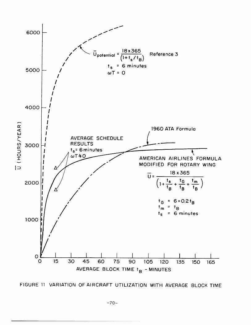
The utilizations achieved are short of the 3000 hours/

year value assumed for costing purposes in the initial

report, Reference 3. Figure 11 shows some typical esti-

mates for variation of utilization with average block time.

The actual results bracket a formula from American Airlines,

which corrects the formula used in Reference 3 by adding

maintenance check time, and a guard time for variability

in operations. The potential utilization would be achieved

when a flight could be started immediately after the end

of the stopping time. The actual utilization shows the

effect of time spent on the ground awaiting a suitable de-

parture time. For example, the average vehicle spends 6.75

hours/day in block time, for the flat demand schedule. It

makes about 27 trips/day and has an assumed total stop time

for load-unload of about 2.7 hours/day. The remainder of an

18 hour useful airline day, or 8.55 hours/day gives 8.55/27 =

19 minutes as the average time spent waiting for a suitable

-71-

departure time. Utilization can be increased at the expense

of load factor by departing early at less suitable times.

The tradeoff is normally not acceptable economically. A

detailed econometric model of the airline market and

schedule is required to ascertain the marginal revenues

and costs involved in such a tradeoff.

There are various ideas which should be investigated

to see their effect on achieving higher utilizations:

1) Change nature of peaking throughout the day.

2) Use smaller vehicles, and average passenger loads.

3) Allow variable load factors throughout the day,

and in low density markets.

4) Split fleet into two vehicle fleets and use

smaller on low density services.

5) Experiment with the optimization algorithm to

improve its effectiveness.

-72-

VII. RESULTING SCHEDULES AND DISCUSSION

The schedules which have been constructed and opti-

mized are too large to be completely shown in this report.

Instead various selected portions are presented to give

some indication of the size and detail of these schedules.

Figures 12 through 15 give the daily schedule for arri-

vals and departures for some of the smaller stations in

the system; Providence, Philadelphia airport, Hartford,

and downtown Boston. Times are given in hundredths of

an hour and NA represents the number of aircraft on the

ground after each time. The schedule construction that

was used for these samples was the peaking distribution

where flights are bunched at 9 and 5 o'clock.

The station schedules give arrivals and departures

for direct flights or services only. They are useful to

give an idea of station loadings to determine personnel

and ground facilities requirements, and the peaking in

passenger flows. Note that NA is not quite correct in

that it describes the time when an incoming arrival could

be ready for departure. The actual arrival occurred 0.10

hours (or 6 minutes) earlier, and the number of gates re-

-73-

quired can be determined using this correction.

However, the listing of arrivals and departures does

not give a complete description of the service to any station,

in the sense that the flights may be continuing flights.

An arrival will represent service from a series of pre-

vious cities. To show complete service is a difficult

task. As an example, Figure 16 shows the service from

the Washington area (two terminals), and includes non-

stop and one-stop flights only. There are 86 services

per day which is slightly less than the present airline

service offered by seven competitors.

Figure 17 shows the schedule for Washington

National airport for the peaking and flat schedules, and

both before and after the optimization for vehicle utili-

zation. They are shown in graphical form with a vertical

time scale so that the peaking effects can be seen, and

both the number of changes of flights, and the extent of

the time changes can be seen. As can be seen, a relatively

few flights are affected, and the time changes involved are

of the order of 6 or 7 minutes. The largest change of time

is 13.2 minutes.

-74-

REFERENCES AND BIBLIOGRAPHY

1. Belmont, Daniel M., "A Pattern of Interstation Air

Travel", Transactions, ASCE, 1957.

2. Lundberg, Bo K. 0., Is Supersonic Aviation Compatible

with the Sound Development of Civil Aviation?, The

Aeronautical Institute of Sweden, Memorandum PE-12,

Stockholm, 1962.

3. M.I.T. Flight Transportation Laboratory, A Systems

Analysis of Short Haul Air Transportation, Cambridge,

Mass., August 1965.

4. Berge, Claude, The Theory of Graphs, Methuen 1962.

5. Ford, L.K. and Fulkerson, D. K., Network Flow Theory,

Princeton, 1962.

6. Moreland, J. A., "Scheduling of Airline Flight Crews",

M.S. Thesis, September 1966, MIT.

7. Levin, A., Crew Scheduling on a Transportation Network,

M. S. Thesis, June 1966, MIT.

-75-

Definitions

Route - a path between a city pair followed by vehicles

in the system, e.g. A B C P Q. A route segment

is a direct link between two cities along a route,

e.g. C P in above example. However, C P itself

is also a route, or direct route for the cities

C and P, so that the terms route and route segment

may be used interchangeably.

Service - the offering of transportation between a city

pair. A specific service is a flight or combina-

tion of flights going between the city pair by any

route. The number of such services per day is called

the Frequency of Service for the city pair, and the

matrix describing frequency of service for all city

pairs is called the Frequency Pattern. In this

report, the frequency of service and frequency pat-

tern shall include only non-stop services. Other

services can be constructed by combining non-stop

services.

-76-

1111111 1 111 IRINJIMIR11ir R111lillIII l" I'll

Flight - a flight is a specific set of services offered

by a vehicle following a given route. A Flight

segment is a direct hop between cities along the

route, and may itself be called a flight or

direct flight. For example, Flight N at 9:00 am

follows route A B C P Q. It provides the fol-

lowing set of services:

Nonstop services A B, B C, C P, P Q

One stop services A C, B P, C Q

Two stop services A P, B Q

Three stop services A Q

Flight segments are A B, B C, C P and P Q. Another

flight Flight M may consist of only one flight

segment, A Q, i.e., a direct flight A to Q.

-77-

Fig. 12 OPERATIONS AT PROVIDENCE

ARRIVALSNA

2

2

2

2

2

2

2

2321

2

1

2

1

2

3

2

21

2

12

1

3

1

2

32

31

2

3

2

1

2

323

2

3

2

1

2

New London

LaGuardia

LaGuardia

Mitchell

LaGuardia

JFK Airport

Mitchell

Boston downtown

New London

LaGuardia

Mitchell

LaGuardia

New BedfordJFK Airport

LaGuardia

TIME073407510752075307540755079307940804080508420865090609070916095509580973100310041016

1026104410451068

DEPARTURESLaGuardiaMitchell

JFK Airport

New Bedford

Boston downtown

New London

LaGuardia

Mitchell

LaGuardiaHartford

JFK Airport

Mitchell

LaGuardia

1069 Boston downtown,New London

10931096113611481187

1196123912521284

12851303

13431366

13781379

1403141715111551155916021674169417131745177617931821

LaGuardiaMitchell

LaGuardiaJFK Airport

Mitchell

LaGuardia

Boston downtownNew London

MitchellLaGuardia

New Bedford

JFK Airport

LaGuardiaMitchell

JFK AirportHartford

LaGuardia

New Bedford

Mitchell

LaGuardia

Boston downtown,New London

JFK Airport

Mitchell

LaGuardia

TIME182218331834184818491871187519001901190619381946195219541958197019941995200120022019

DEPARTURES

New London

Boston downtown

LaGuardia

Mitchell

JFK AirportLaGuardia

Mitchell

LaGuardia

Boston downtown

New London

LaGuardia

LaGuardia

Mitchell

Boston downtown

New London

JFK Airport

New Bedford

LaGuardia

Mitchell

LaGuardia

Hartford

JFK Airport

Boston downtown,Mitchell

20712076207821132122

2124214321512161

2202

2217

22342241

22842285

230523322356

LaGuardia

Mitchell

New Bedford

LaGuardia

Boston Downtown,New LondonJFK Airport

Mitchell

LaGuardia

-78-

NA ARRIVALS1

2 Mitchell

12 Boston downtown12 New London

12 LaGuardia

1

01 Mitchell

01 JFK Airport01 LaGuardia01 Mitchell0

1 LaGuardia

02 Boston downtown,

New London10

1 LaGuardia0

1 Mitchell

2022 Mitchell2025 JFK Airport20612062 Hartford

2070

IIIIIII II 11111 Iml IIIIIIIIIII FIJI 1.11111111, 1 ' IF,11,111 11 1 , 11 1 1 111 iiiiN i III III IW III

Fig. 13 OPERATIONS AT PHILADELPHIA AIRPORT

NA ARRIVALS

5

5 Philadelphiadowntown

432

1

3 Wilmington,LaGuardia

2 Baltimore

13 Washington, DC

Mitchell1

2 JFK Airport12 New York

3 N.Y. TeterboroAirport

2

3 Stamford,Greenwich

4 Newark6 Lancaster, Phila-

delphia downtown5

TIME DEPARTURES


0728 LaGuardia

0731 Baltimore0738 Washington,DC0741 Mitchell0742 Wilmington

0751

0752 JFK Airport,Newark

0766

07700778

New York

NA ARRIVALS

New York

Washington, DC

Philadelphiadowntown

Wilmington

N.Y. Teterboro

AirportMitchell

3 Stamford Greenwich

4 LaGuardia

0779 NY Teterboro

Airport, Stamford,Greenwich

080108050$060817

Lancaster


0823

0826

0833

0851 LaGuardia

Newark

Baltimore

TIME DEPARTURES

09971002100510061012

Wilmington

Philadelphia

1013 LaGuardia

10211022

1025

10261028

1031

1051

105710621063

Newark

Baltimore

Lancaster

1064 Philadelphia

downtown1065 Washington, i

1072 Mitchell


1078

1083 JFK Airport1091 LaGuardia

1102 Wilmington

2 LaGuardia

3 Baltimore

23 Philadelphia

downtown4 Wilmington5 Washington, DC6 Mitchell5432

12 Philadelphia

downtown1

2 LaGuardia

3 JFK Airport3 Baltimore

085808740884

0888

0889

0893

08950902

0914091709230935093909460949

09610963

09720973

097709810987

BaltimoreWashington, DCMitchell

Philadelphia

Washington, DC

JFK Airport

2 Mitchell

Wilmington

LaGuardiaJFK AirportBaltimorePhiladelphiadowntownNew York

Washington, DC

Stamford,Greenwich 1Mitchell, N.Y. 3Teterboro Airport 4

3

2 LaGuardia3 Wilmington


5 Baltimore6 New York

1


Washington, DC

LaGuardia, N.Y.Stamford, Greenwich

1108111211211122

1123

Baltimore

New York

1124 Philadelphia

downtown11291134

1138

114711581164 Washington, DC

1175 LaGuardia, NYTeterboro Airport,Stamford, Green-wich


1198

11991203

1204121312191232

Mitchell

Baltimore

Wilmington

-79-

Fig. 13 OPERATIONS AT PHILADELPHA AIRPORT (cont'd)

NA ARRIVALS TIME

4 Mitchell5 Baltimore4

33 Wilmington

23 Philadelphia

downtown23 JFK Airport4 Newark

5 LaGuardia434 Washington, DC3

2

3 Baltimore4 New York


45 Mitchell4

34 Lancaster5 Wilmington6 LaGuardia53

2

1


3 Washington, DC4 NY Teterboro

Airport3

4 Stamford,Greenwich

5 Baltimore6 JFK Airport5

123812391244

DEPARTURES

JFK Airport

1252 Newark1260 Philadelphia

downtown1272 LaGuardia1274

128112821287

13101313132113241334

NA ARRIVALS TIME DEPARTURES

41

2 Wilmington4 Newark, Baltimore

5 New York

6 Washington, DC

Washington, DC


BaltimoreNew York

Mitchell


1348135'11358

136313731392

1406140714251430

Lancaster

LaGuardia

Wilmington

1435 Washington,DC1441 N.Y. Teterboro



1458 Baltimore

1463

14781479

1482 JFK Airport

1485

149315201533 Mitchell

1565 LaGuardia

Mitchell

5 LaGuardia6 Philadelphia

downtown5

15721594

16031608


1658 Newark

LaGuardia

0

1 Mitchell1 Philadelphia

2 JFK Airport12 Baltimore

12 Wilmington12 N.Y. Teterboro

Airport1

2 Stamford, Green-wich

Washington, DC

2 Lancaster

2 Philadelphia down-town

3 LaGuardia212 Mitchell

New York

3 Philadelphiadowntown, Baltimore

1674 Wilmington1694 Baltimore, Wash-

ington, DC, N.Y.17131729

1730

1737


1770 LaGuardia

1784 Mitchell1797 Baltimore1805 JFK Airport

18081811 NY Teterboro

Airport1816 Lancaster


18211822

182318241835

1836184018411849

Stamford, Green-wich

Washington, DC

Wilmington

LaGuardia

1850 Mitchell

1860


18671871

1873

18741875

187918881891189318941896

New York

Baltimore

Washington, DCLaGuardia

Newark


1905

-80-

Fig. 13 OPERATIONS AT PHILADELPHIA AIRPORT (cont'd)

NA ARRIVALS

2 LaGuardia1

0

2 Wilmington,Washington,DC

JFK Airport

2 Newark, Phila-delphia downtown

Baltimore

Mitchell


1

2 LaGuardia

1

2 Stamford, Green-wich

0

1 Philadelphia dntn

1 Washington, DC

1 Wilmington

New York

Baltimore

TIME DEPARTURES

1906 Wilmington,JFK Airport

19141915 Baltimore


1925

1926 Mitchell1932

1933 NY TeterboroAirport

1936 Washington, DC

19371958

19591963

LaGuardia

Stamford, Greenwich


1965 New York

1968

19691970

Wilmington

1971 Baltimore, JFK

Airport

1976

1982 Mitchell

1983 LaGuardia

198619871991

19981999


1 LaGuardia

2 Lancaster2 JFK Airport

Mitchell

1 Washington, DC

02 Wilmington, Phila-

delphia downtown

0

1 Baltimore

Washington, DCPhiladelphiadowntown

NA ARRIVALS

1 Newark

LaGuardia

1 NY TeterboroAirport

1 Mitchell01 Philadelphia

downtown

01 Stamford, Green-

wich

2 Washington, DC3 New York

4 Baltimore

5 JFK Airport

4

5 LaGuardia4

33 Wilmington


3

2

3 Mitchell4 Washington, DC

5 Baltimore2

5 LaGuardia6 Philadelphia

downtown

Lancaster

Lancaster

2013

2021 Baltimore

20232025

203120342036

2037204120452048

Newark

LaGuardia

PhiladelphiadowntownWilmington

Mitchell

2049 N.Y. Teterboro


2056

2 Newark


2

3 Stamford, Green-

wich

4 New York323 JFK Airport

3 Wilmington,

21

2 Mitchell

4 Baltimore, Wash-

ington, DC


6 LaGuardia

TIME DEFPAR'PTURES

2060 Washington, DC

2069 New York2074 Philadelphia

downtown2079

2080 Baltimore

208420852088

20892093

JFK Airport

LaGuardia

21032105211521232124 Wilmington

2127


2134 Mitchell

2143 Washington, DC

2144

215921662173218621942200

22042214

2217222222452247

2258

226822692285

22902291

22942296230123062309

23132331

23352344

2345

2351

BaltimoreLaGuardia


Lancaster

Newark

N.Y. TeterboroAirport, Stamford,GreenwichNew York

JFK Airport

Wilmington

MitchellWashington, DC

Baltimore

LaGuardiaPhiladelphiadowntown

-81-


Fig. 14 OPERATIONS AT HARTFORD

NA ARRIVAL.S TIME DEPARTURES NA ARRIVALS

0710 New Haven

TIME DEPARTURES

1252 Boston Logan,New York

2 New Haven

3 Hartford, Brad-field

2

3 LaGuardia21

2 Scranton3 Boston Logan


5 Newark

6 Boston downtown

54

5 New Haven

434 LaGuardia

5 Hartford

432

3 New Haven

1

2 Providence

Scranton


LaGuardia

07340741074907570767

Hartford Bradfield,4

LaGuardia 3

Newark 4

56

New Haven

Boston LoganNewarkHartford


077907830791082608290831

0832084108590884

08880890089509220923

Boston downtown

Boston Logan

New Haven

LaGuardia

HartfordScranton

0941 Waterbury

0958 New Haven0961 Philadelphia

downtown

0981

0987 Providence,LaGuardia

10021003

1008

Boston Logan

1009 Hartford, Brad-field

1021

10221025

LaGuardiaScranton


New HavenBoston downtown

Hartford Brad-field

LaGuardiaNew Haven

Boston Logan

NewarkScranton


4

34 New Haven

5 Hartford,Brad--field

6 LaGuardia

Newark

1032 Boston downtown

Hartford Bradfield

Boston Logan

NewarkNew Haven

Boston downtown

LaGuardia1131

Waterbury 1135

1136

New Haven 1159

Hartford Bradfield 1164

Scranton 1178Philadelphia down- 1183town

LaGuardia

119912371239

1042104510601063106810881105

New Haven

LaGuardia

1122 Philadelphiadowntown, Scran-ton

1126Hartford Brad-

New Haven

LaGuardia

New Haven

New Haven

Boston downtown

LaGuardia

Hartford Brad-field

12621278129012931311

Hartford

1321 Philadelphiadowntown, Scranton

1334 LaGuardia

1366 New Haven1372

1377

1379 Boston downtown1382

138914151494 Hartford,Bradfield

1527

1533 LaGuardia

1551 New Haven

157115741694 Boston Logan, Newark,

Philadelphia down-

town, Scranton1732

17351750

1755

1776 Hartford, Brad-field, New Haven

1784 LaGuardia1799

1809

1822

1828 Boston downtown

1852 New Haven1865 Hartford Bradfield,

LaGuardia1868 Philadelphia

downtown

1870187118771878189418951898

Scranton

Boston Logan

Newark

1907 New Haven

Scranton

New Haven


Newark

Boston Logan

LaGuardia

1924192519301932

1934194219451955

195819641965

-82-

LaGuardia

Hartford Bradfield

Waterbury

New Haven

Philadelphiadowntown, Scranton

NA ARRIVALS TIME DFPARTURES

Fig. 14 OPERATIONS AT HARTFORD (cont'd)


2 Hartford Bradfield 19673 New Haven 19812 1984 LaGuardia

1 1995 Boston downtown2 Scranton 19961 1997 Boston Logan2 LaGuardia 20091 2010 New HavenU 2022 Hartford Bradfield1 Philadelphia 2024

downtown0 2025 Newark1 Boston downtown 20312 New Haven 20330 2049 Providence, LaGuardia1 Hartford Bradfield 20552 Newark 20663 Waterbury 20681 2069 Philadelphia downtown,

Scranton0 2071 New Haven1 Boston Logan 20742 Providence 20913 LaGuardia 20924 New Haven 20943 2096 Hartford Bradfield4 Scranton 21255 Hartford Bradfield 21296 Philadelphia down- 2130

town5 2134 LaGuardia4 2151 New Haven5 LaGuardia 21726 New Haven 21745 2217 Boston downtown4 2226 Newark3 2234 Boston Logan4 Boston downtown 22532 2258 Philadelphia down-

town, Scranton1 2267 Hartford, Bradfield2 Boston Logan 22723 Newark 22752 2296 LaGuardia3 Hartford Bradfield 23002 2305 New Haven3 Scranton 23144 Philadelphia down- 2319

town5 New Haven 23286 LaGuardia 2334

-83-

Fig. 15 OPERATIONS AT BOC - BOSTON ON THE CHARLES

k ARRIVALS

Boston Logan

LaGuardia

Mitchell,Newark

ProvidenceHartford

WorchesterJFK AirportPhiladelphiaLaGuardia

TIME0614065606690670

0675069107040805

0818081908200847086608740880

DEPARTURESLaGuardiaBoston LoganProvidenceNewark,MitchellField

Philadelphia

JFK Airport,Hartford

LaGuardiaWorchester

0888 LaGuardia

0922 Boston Logan

Boston LoganLaGuardia

LaGuardiaMitchell

Newark

Boston Logan

LaGuardiaHartford

ProvidencePhiladelphiaLaGuardia

JFK Airport

WorchesterMitchellBoston LoganLaGuardiaNewark

Boston Logan

LaGuardia

LaGuardiaPhiladelphia

093609490957096110061010101910221025103410441063106410671068

1069

108810931105112111221123112411641180118411851186118812041249

1252126013211335

LaGuardiaNewarkMitchellLaGuardia

Philadelphia

Boston LoganProvidence

LaGuardia

JFK Airport,fordWorchester

Hart- 2

Newark, Mitchell

LaGuardia

LaGuardia

PhiladelphiaLaGuardiaNewark,Mitchell

1344 Logan1354 Providence

NewarkPhiladelphia

LaGuardia

Boston Logan

Providence

LaGuardia

Hartford

JFK Airport

LaGuardia

Mitchell

NewarkBoston Logan

LaGuardia

WorchesterPhiladelphia

LaGuardiaProvidence

7ogan, Mitchell

TIME1368136913781379

1403140514151440

1449151015941636165516701693

DEPARTURES

Boston Logan

JFK Airport,Hartford

NP ARRIVALS2 Boston Logan1

3 Newark,Mitchell1

2 Providence3 LaGuardia4 Hartford5 JFK Airport

45 LaGuardia4

3

4 LaGuardia3

5 Boston Logan,Worchester

1

2 Fitchburg Air-port

3 Mitchell

1694 Boston Logan,Newark, Mitchell,Philadelphia

1751

175217561758177718151817182018241841185018511858185918601861

1864

186518891900190119141915192919311935194419551958196019621963

1964199219941995

20052006

LaGuardia

LaGuardia

JFK AirportProvidenceHartford

Boston Logan

LaGuardia

Newark

MitchellLaGuardia

Philadelphia

Boston Logan

LaGuardia

Worchester

Newark

JFK Airport,MitchellLaGuardia

Providence,Hartford

Boston Logan,

LaGuardia

-84-

LaGuardia

LaGuardiaFitchburg Airport

Worchester

Fig. 15 OPERATIONS AT BOC - BOSTON ON THE CHARLES (cont'd)


1 LaGuardia 2025 Philadelphia1 Newark 20292 Hartford 20311 2036 LaGuardia2 JFK Airport 20563 LaGuardia 20601 2069 Newark,Mitchell

0 2078 LaGuardia1 LaGuardia 20970 2100 Boston Logan1 Philadelphia 21082 Boston Logan 21143 Mitchell 21272 2130 LaGuardia

3 Newark 21334 LaGuardia 21393 2172 JFK Airport

4 LaGuardia 21913 2193 Worchester

2 2200 LaGuardia

0 2217 Providence,Hartford

1 Worchester 2218

0 2234 Philadelphia

1 Providence 2241

2 Hartford 2253

0 2258 Newark,Mitchell

1 LaGuardia 2261

0 2277 Boston Logan

1 JFK Airport 2278

2 Boston Logan 2291

3 Mitchell 2316

4 Philadelphia 2317

5 Newark 2322

4 2331 LaGuardia

5 LaGuardia 2392

-85-

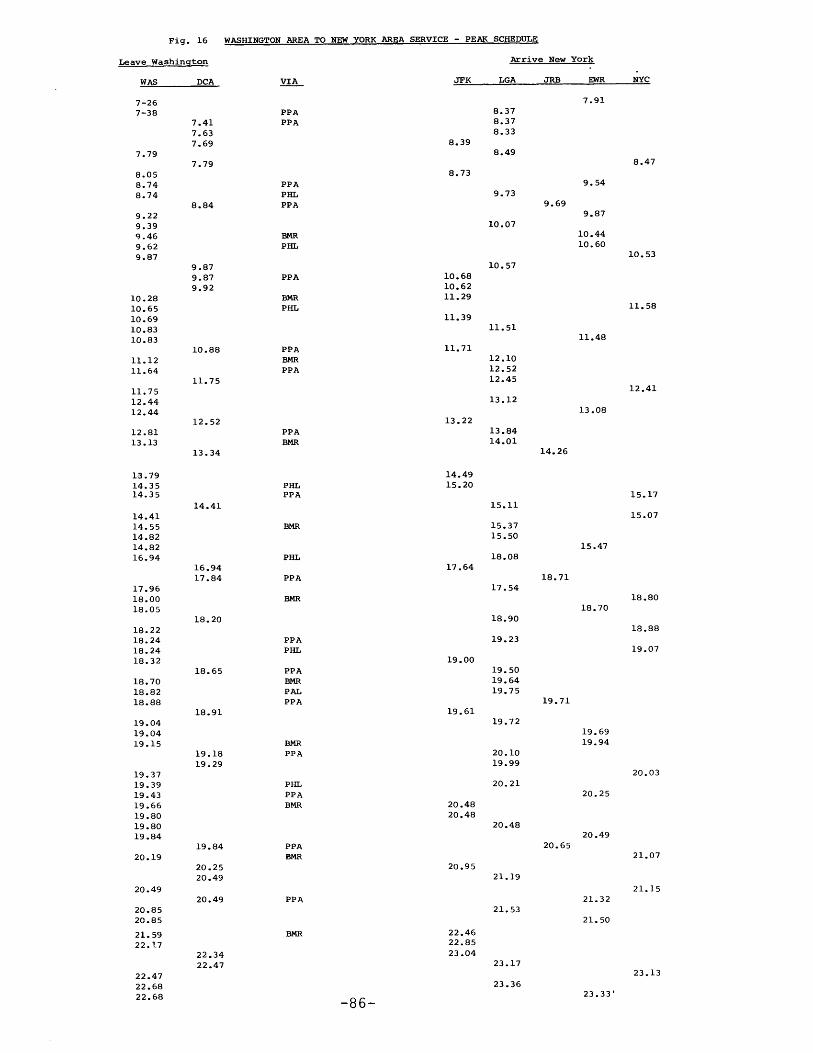
TO NEW YORK AREA SERVICE - PEAK SCHEDULE

Leave Washington

WAS DCA

7-267-38

7.79

8.058.748.74

9.229.399.469.629.87

10.2810.6510.6910.8310.83

11.1211.64

11.7512.4412.44

12.8113.13

13.7914.3514.35

14.4114.5514.8214.8216.94

17.9618.0018.05

18.2218.2418.2418.32

18.7018.8218.88

19.0419.0419.15

19.3719.3919.4319.6619.8019.8019.84

20.19

20.49

20.8520.85

21.5922.17

22.4722.6822.68

7.417.637.69

7.79

8.84

9.879.879.92

10.88

11.75

12.52

13.34

14.41

16.9417.84

18.20

18.65

18.91

19.1819.29

19.84

20.2520.49

20.49

VIA

PPAPPA

Arrive New York

JFK LGA JRB EWR NYC

7.918.378.378.33

8.398.49

8.73

9.73PPAPHLPPA

BMRPHL

PPA

BMRPHL

PPABMRPPA

10.6810.6211.29

11.39

11.71

13.22

14.4915.20PHL

PPA

PHL

PPA

BMR

PPAPHL

PPABMRPALPPA

BMRPPA

PHLPPABMR

PPABMR

PPA

17.64

19.00

19.61

20.4820.48

20.95

22.4622.8523.0422.34

22.47

10.07

10.57

11.51

12.1012.5212.45

13.12

13.8414.01

15.11

15.3715.50

18.08

17.54

18.90

19.23

19.5019.6419.75

19.72

20.1019.99

20.21

20.48

21.19

21.53

23.17

23.36

-86-

8.47

9.69

9.54

9.87

10.4410.60

10.53

11.58

11.48

12.41

13.08

14.26

15.17

15.07

15.47

18.71

18.7018.80

18.88

19.07

19.71

20.65

19.6919.94

20.25

20.49

21.32

21.50

20.03

21.07

21.15

23.13

23.33

Fig. 16 WASHINGTON AREA

FIG. 17 TYPICAL STATION SCHEDULES - WASHINGTON NATIONAL

112 OPERATIONS PER DAY - TO AND FROM NEW YORK JFK,NEW YORK LGA, WASHINGTON DOWNTOWN, RICHMOND, PHILADELPHIA DOWNTOWN

FLAT DEMAND

Revisions inFinal Schedule

NAC TIME

4

NAC

5

WAS -

PPA

RIC

LGAJFKWAS

PPA

WAS

DUL

PPA

LGARIC

JFK

WAS

PPA

WAS

LGAPPA

WASRIC

JFK

WASPPA

LAWASPPA

R IC

WASJFK

PPA

WAS

LGA

PPA

WAS

R IC

J FK

WASPPA

LGA

WAS

PPA

WASRIC

DULJFK

PPA

LGAWAS

PPAWAS

R ICWASJFKLGAPPA

5

PPA

LGA --

WASPPA

. WASPPA

LGAJ JFK, RIC

WAS

PPA

WAS

DUL, LGA, PPA

WASJFK,RIC

PPAWAS

LGA, WAS

PPA

JFK, RIC

WAS

PPA

WAS

LGA

PPAWAS

JFK, RIC

WAS

PPA

LGA

WAS

-+PPA

- WAS

JFK, RIC

PPA

LG A, WAS

p ~S

JFK,RICWAS

DUL, LAG, PPA

- WAS

- PPA

- WAS

JFK, RICLIDA

PPAWAS

R IC --.-

WAS E.W

RIC

WAS

LGA

LGADUL

-. RIC

==* JFK

WAS

WAS

WAS

LGA

RIC

WAS

LGA

DULLGA

PPA

WAS

DUL

WASPPALGARIC

JFK

PPA

WAS

PPA ,LA

WASRIC

JFK

PPA

WAS

LGA

PPA, WAS

RIC

JFK

WAS

PPA

WAS

LGAWASPPARICWAS

PFA, JFK

WASLEAPPA

WAS

AOL

JFK, PPAWASLEA

PPA, WAS

RICLA

PEAKED DEMAND

Original Revisions inSchedule Final Schedule

WAS

PPA

LGAJFK,RIC

WAS

PPA

WAS

DUL, LGA,PPAWASJFK, RIC WAS ___;

PPAWAS

DUL RIC

4

TIME

0600

0630

0700

0730

0800

0830

-0930

'0[00

I030

1100

1130

1200

1230

1300

1330

1400

1430

1500

1530

1600

1630

1700

1730

1800

1830

1900

j930

2000

2030

2100

2130

2200

2230

2300

2330

2400

JFK

JFK

WAS

DUL

-87-

OriginalSchedule

WASRICJFK

APPENDIX A

An Extension of the Network Models to Include Time of Day

A more useful class of network models dealing with trans-

portation problems is defined by extending the geometry of

the network into a time dimension. In the geographic model

used to describe passenger flow, a node represented a point

in geographic dimensions (latitude and longitude, for ex-

ample). The flow in the network, X, was posed as passengers

per day. In this appendix, an extension of this problem is

shown where each node now represents a point in both space

and time. The passengers are now travelling least time

paths along specified individual flights, and making flight

connections as appropriate. There are many other uses for

such space-time models in flight scheduling. References 6

and 7 describe some applications in the area of flight

crew scheduling.

Figure 19 shows a simple model of the Time of Day network

model. Stations A, B, C etc. are listed across the page,

with a vertical line beneath each station representing the

time dimension. Nodes along the station line represent a

point in time; e.g. A0600, A0900, etc. These station time

nodes are joined by station transit arcs of unlimited capacity

-89-

whose cost is a time proportional to the time difference

of its nodes. The flow in these arcs represents passen-

gers waiting for a suitable departure, and they incur

transit ground time costs in waiting.

The service network now consists of every individual

flight hop as specified by the schedule construction pro-

cess. The service arcs are a given flight (e.g. A0900 to

C1000) with unlimited capacity, and a time cost equal to

flight time plus unloading time. The service network is

now a routing diagram commonly used by graphical schedu-

ling methods.

At each flight arrival node, a disembarc goes to the

station node (e.g., arrivals at C are connected to C*).

The disembarcs have unlimited capacity, and a penalty cost

of the order of 24 hours. The flow on the set of disem-

barcs represents people leaving the station throughout

the day.

The demand arcs (e.g. D* A0600, D* A0900) distribute

the demand between stations throughout the day. The capa-

cities are set to the estimated demand values, and the

demand arcs costs are zero. The daily variations in demand

are represented by the discrete inputs of demand at any time

interval desired (e.g. hourly). The demand arc creates a

need for a flow through the service network along the path

-90-

0600

0900

I iI gI I| II II |I I

I I

I ~ 24(

I T

StationTransitArcs

Flight Arcs

Disemborcs

0600

2400

ine of Day Demand Arcs

FIGURE 19 A TIME OF DAY TRANSPORTATION NETWORK

)00

which gives least overall trip time.

With the model formulated above, the computer methods

used in the geographic model are applicable. The flow

solution, X, would describe the number of passengers on

board each flight and the number of people on the ground

in each station awaiting a departure. A review of pas-

senger load sizes would indicate desirable vehicle size

and allow computation of load factor distributions. Any

individual flight can be changed in time, and the effect

on passenger load noted.

This model has not been exercised on the Northeast

Corrider Airbus example. It would be a very large network

with some 55000 arcs, and would require reprogramming to

handle input of the demand information. It is presented

as an example of the use of more detailed network models

in schedule planning or schedule control. It can be con-

ceived as a technique to be used in a modal competition

problem. For time sensitive passengers, a model having

the service networks for each mode, suitably interconnected

by transfer arcs for one mode to another at a given city

can be constructed, and the passenger flows on each mode

obtained. Similar flow solutions can be obtained for cost

-92-

sensitive passengers, etc. Each mode can then revise

its service network to operate more efficiently, or to

capture passengers away from other modes. Such a model

can also be applicable to study the competition between

carriers in a given mode of transportation.

No capacity constraints have been applied to flight

service arcs. Such a flow problem is known as the capa-

citated multi-commodity flow problem for which suitable

integer methods of solution do not exist as yet.

-93-

'COMPUTERIZED SCHEDULE CONSTRUCTION FOR AN AIRLINE ...

Documents

Transcript of 'COMPUTERIZED SCHEDULE CONSTRUCTION FOR AN AIRLINE ...