
Computer Vision Projective Geometry and · PDF fileto the 6 extrinsic parameters needed for...
83
10/17/09 CS 461, Copyright G.D. Hager Computer Vision Projective Geometry and Calibration Professor Hager http://www.cs.jhu.edu/~hager Jason Corso http://www.cs.jhu.edu/~jcorso .
Transcript of Computer Vision Projective Geometry and · PDF fileto the 6 extrinsic parameters needed for...

10/17/09 CS 461, Copyright G.D. Hager
Computer Vision Projective Geometry
and Calibration Professor Hager
http://www.cs.jhu.edu/~hager
Jason Corso http://www.cs.jhu.edu/~jcorso
.

Topics
• Camera projection models
• Spatial transformations
• Projective coordinates
• Camera calibration
10/17/09 CS 461, Copyright G.D. Hager

10/17/09 CS 461, Copyright G.D. Hager
Pinhole cameras
• Abstract camera model - box with a small hole in it
• Pinhole cameras work in practice

10/17/09 CS 461, Copyright G.D. Hager
Real Pinhole Cameras
Pinhole too big - many directions are averaged, blurring the image
Pinhole too small- diffraction effects blur the image
Generally, pinhole cameras are dark, because a very small set of rays from a particular point hits the screen.

10/17/09 CS 461, Copyright G.D. Hager
The reason for lenses
Lenses gather and focus light, allowing for brighter images.

10/17/09 CS 461, Copyright G.D. Hager
The thin lens
1z'−1z=1f
Thin Lens Properties: 1. A ray entering parallel to optical axis
goes through the focal point. 2. A ray emerging from focal point is parallel
to optical axis 3. A ray through the optical center is unaltered

10/17/09 CS 461, Copyright G.D. Hager
The thin lens
1z'−1z=1f
Note that, if the image plane is very small and/or z >> z’, then z’ is approximately equal to f
10/17/09 CS 461, Copyright G.D. Hager
Field of View
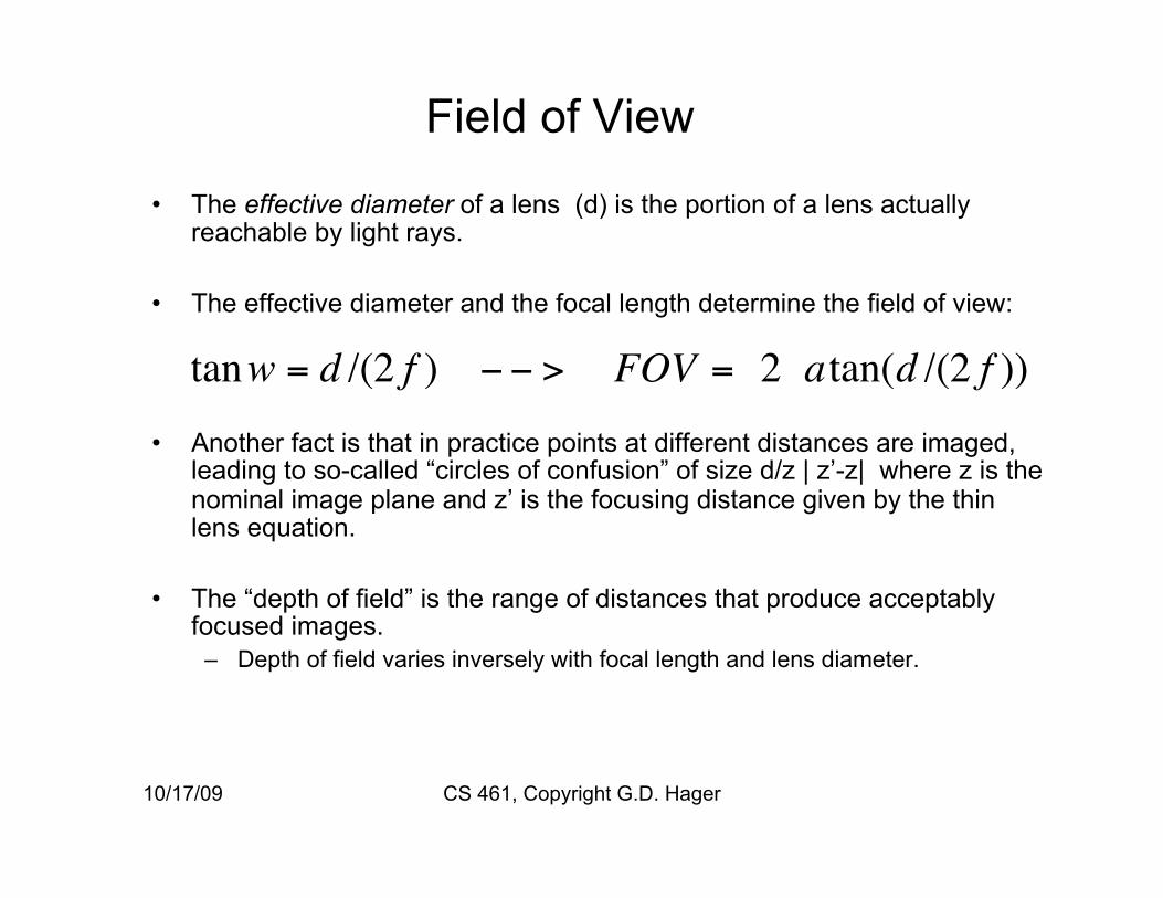
• The effective diameter of a lens (d) is the portion of a lens actually reachable by light rays.
• The effective diameter and the focal length determine the field of view:
• Another fact is that in practice points at different distances are imaged, leading to so-called “circles of confusion” of size d/z | z’-z| where z is the nominal image plane and z’ is the focusing distance given by the thin lens equation.
• The “depth of field” is the range of distances that produce acceptably focused images.
– Depth of field varies inversely with focal length and lens diameter.
€
tanw = d /(2 f ) −− > FOV = 2 atan(d /(2 f ))

10/17/09 CS 461, Copyright G.D. Hager
Lens Realities Real lenses have a finite depth of field, and usually
suffer from a variety of defects
vignetting
Spherical Aberration

10/17/09 CS 461, Copyright G.D. Hager
Perspective Projection
• Equating z’ and f – We have, by similar triangles,
that (x, y, z) -> (-f x/z, -f y/z, -f) – Ignore the third coordinate, and
flip the image around to get:
(x, y, z)→ ( f xz, f yz)

10/17/09 CS 461, Copyright G.D. Hager
Distant objects are smaller

10/17/09 CS 461, Copyright G.D. Hager
Parallel Lines Meet at a Point
common to draw film plane in front of the focal point
A Good Exercise: Show this is the case!

The Projection “Chain”
10/17/09 CS 461, Copyright G.D. Hager
Transform to camera
coordinates
Projection Conversion to Pixel Grid
Points in the world
Points in the image

10/17/09 CS 461, Copyright G.D. Hager
Intrinsic Parameters
Intrinsic Parameters describe the conversion from unit focal length metric to pixel coordinates (and the reverse)
umm = f x/z vmm = f y/z
umm = (upix – ox) su --> 1/su umm + ou = upix vmm = (vpix – oy) sv --> 1/sv vmm + ov = vpix
It is common to combine scale and focal length together as the are both scaling factors; note projection is unitless in this case!

The Projection “Chain”
10/17/09 CS 461, Copyright G.D. Hager
Transform to camera
coordinates
Projection Conversion to Pixel Grid
Points in the world
Points in the image

10/17/09 CS 461, Copyright G.D. Hager
Projection Geometry: Standard Camera Coordinates
• By convention, we place the image in front of the optical center – typically we approximate by saying it lies one focal distance from the center – in reality this can’t be true for a finite size chip!
• Optical axis is z axis pointing outward
• X axis is parallel to the scanlines (rows) pointing to the right!
• By the right hand rule, the Y axis must point downward
• Note this corresponds with indexing an image from the upper left to the lower right, where the X coordinate is the column index and the Y coordinate is the row index.

10/17/09 CS 461, Copyright G.D. Hager
An Aside: Geometric Transforms
In general, a point in n-D space transforms rigidly by
newpoint = rotate(point) + translate(point)
In 2-D space, this can be written as a matrix equation:
+
−=
tytx
yx
CosSinSinCos
yx
)()()()(
''
θθ
θθ
In 3-D space (or n-D), this can generalized as a matrix equation:
p’ = R p + T or p = Rt (p’ – T) Transforming the observer frame Transforming the world frame

10/17/09 CS 461, Copyright G.D. Hager
Properties of Rotations
• In general, a rotation matrix satisfies two properties: – Rt R = R Rt = I – det(R) = 1
• What does this make the inverse of a rotation?
• Note that this defines some properties of the component vectors of the matrix.
• A 3D rotation can be expressed in many ways: – as a composition of individual rotations R3d(θ1, θ2, θ3) = R2d(θ1) R2d(θ2) R2d(θ3) – as an angle-axis n, θ
R = I cos(θ) + (1-cos(θ)) (n nt) + sin(θ) sk(n)

10/17/09 CS 461, Copyright G.D. Hager
Homogeneous Transforms
Now, using the idea of homogeneous transforms, we can write:
p ' =R T
0 0 0 1
p
R and T both require 3 parameters. These correspond to the 6 extrinsic parameters needed for camera calibration
Often, we want to compose transformations, but using separate translations and rotations makes that clumsy.
Instead, we embed points in a higher-dimensional space by appending a 1 to the end (now a 4d vector)

How Do We Combine Projection and Transformation?
• Step 0: Points are expressed in some coordinate system that is not the cameras (e.g. a model or a robot): – p = (x, y, z ,1)
• Step 1: Transform the points into camera coordinates – q= (x’, y’, z’, 1) = T p
• Step 2: Project the points – u = f x’/z’ ; v = f y’/z’
• A linear step followed by a nonlinear step …
10/17/09 CS 461, Copyright G.D. Hager

10/17/09 CS 461, Copyright G.D. Hager
Basic Projective Concepts
• We have seen homogeneous coordinates already; projective geometry makes use of these types of coordinates, but generalizes them
• The vector p = (x,y,z,w)’ is equivalent to the vector k p for nonzero k – note the vector p = 0 is disallowed from this representation
• The vector v = (x,y,z,0)’ is termed a “point at infinity”; it corresponds to a direction
• We can embed real points into projective space, and always recover the “real” point by normalizing by the third coordinate provided it is not a point at infinity.
• A good model for P(n) embedded in R(n+1) is the set of all lines passing through the origin – each line corresponds to a point

10/17/09 CS 461, Copyright G.D. Hager
The Camera Matrix
• Homogenous coordinates for 3D – four coordinates for 3D point – equivalence relation (X,Y,Z,T) is the same as (k X, k Y, k Z,k T)
• Turn previous expression into HC’s – HC’s for 3D point are (X,Y,Z,T) – HC’s for point in image are (U,V,W)
UVW
=
1 0 0 00 1 0 00 0 1
f 0
XYZT
),(),(),,( vuWV
WUWVU =→

10/17/09 CS 461, Copyright G.D. Hager
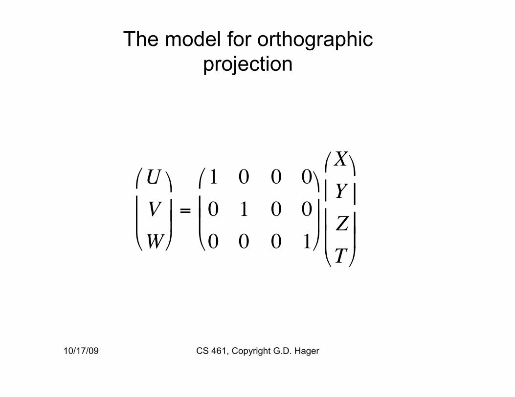
Orthographic projection
yvxu
=
=Suppose I let f go to infinity; then
10/17/09 CS 461, Copyright G.D. Hager
The model for orthographic projection
UVW
=
1 0 0 00 1 0 00 0 0 1
XYZT

10/17/09 CS 461, Copyright G.D. Hager
Scaled Orthography (Weak Perspective)
• Issue – perspective effects, but not over
the scale of individual objects – collect points into a group at
about the same depth, then divide each point by the depth of its group
– Adv: easy – Disadv: wrong
*/ Zfssyvsxu
=
=
=

10/17/09 CS 461, Copyright G.D. Hager
The Model for Scaled Orthography
=
TZYX
fZWVU
/*00000100001

Affine Projection
10/17/09 CS 461, Copyright G.D. Hager
Pick an arbitrary point p0 = (x0,y0,z0)t
Recall u = f x/z and v = f y /z
Linearize about p u = f/z0 (x-x0) – f x0/z02 (z-z0)
u = [f/z0 0 f x0/z02 f x0/z0 – f x0/z0]
€
UVW
=
1 0 x0 /z0 00 1 y0 /z0 00 0 0 z0 / f
XYZT

10/17/09 CS 461, Copyright G.D. Hager
Intrinsic Parameters
Intrinsic Parameters describe the conversion from unit focal length metric to pixel coordinates (and the reverse)
xmm = - (xpix – ox) sx --> -1/sx xmm + ox = xpix ymm = - (ypix – oy) sy --> -1/sy ymm + oy = ypix
pKwyx
osos
wyx
mm
yy
xx
pix
int
100/100/1
=
−
−
=
or
It is common to combine scale and focal length together as the are both scaling factors; note projection is unitless in this case!

10/17/09 CS 461, Copyright G.D. Hager
Putting it All Together Now, using the idea of homogeneous transforms, we can write:
p ' =R T
0 0 0 1
p
R and T both require 3 parameters. These correspond to the 6 extrinsic parameters needed for camera calibration
Then we can write
q = Π p’ for some projection model Π
Finally, we can write
u = K q for intrinsic parameters K

10/17/09 CS 461, Copyright G.D. Hager
Camera parameters • Summary:
– points expressed in external frame – points are converted to canonical camera coordinates – points are projected – points are converted to pixel units
=
TZYX
WVU
parameters extrinsicngrepresenti
tionTransforma
model projectionngrepresenti
tionTransforma
parameters intrinsic ngrepresenti
tionTransforma
point in cam. coords.
point in metric image coords.
point in pixel coords.
point in world coords.

Some Things to Point Out
10/17/09 CS 461, Copyright G.D. Hager
General projection model: q = λ K Π H p = λ Mp
If M is perspective, 3x4 values-> how many independent parameters?
If M is affine, how many independent parameters?
If M is orthographic, how many independent parameters?

What Is Preserved?
• We are used to rigid body transformations (homogeneous transforms) which preserve: – Distance – Angle – Area
• With Affine, we lose distance and length; what is preserved is – Ratios of distances/lengths – Area
• With Projective, we also loose preservation of area; what is preserved is: – Ratios of ratios of distances (the so-call cross-ratio) – Intersection/coincidence of lines/points
10/17/09 CS 461, Copyright G.D. Hager

10/17/09 CS 461, Copyright G.D. Hager
Model Stratification Euclidean Similarity Affine Projective
Transforms rotation x x x x translation x x x x uniform scaling x x x nonuniform scaling x x shear x x perspective x composition of proj. x Invariants length x angle x x ratios x x parallelism x x x incidence/cross rat. x x x x

10/17/09 CS 461, Copyright G.D. Hager
Projection and Planar Homographies
• First Fundamental Theorem of Projective Geometry: – There exists a unique homography that performs a change of basis
between two projective spaces of the same dimension.
– Projection Becomes
– Notice that the homography H is defined up to scale (s).

10/17/09 CS 461, Copyright G.D. Hager
Estimating A Homography
• Here is what looks like a reasonable recipe for computing homographies: – Planar pts (x1;y1;1, x2; y2; 1, .... xn;yn;1) = X – Corresponding pts (u1;v1;1,u2;v2;1,...un;vn;1) = U – U = H X – U X’ (X X’)-1 = H
• This will not work: the problem is really λi Ui = H Xi
• So we’ll have to work a little harder ... – hint: work out algebraically eliminating λi

10/17/09 CS 461, Copyright G.D. Hager
Properties of SVD • SVD: A = U D Vt
– U and V are unitary (unit columns mutually orthogonal, but not rotations!) – D is diagonal – In general if A = m x n, U is mxm, D is m x n, V is n x n – If m > n, there will be many zeros in D; can make U mxn and D nxn – Eigenvalues are squares of elements of D; eigenvectors are columns of V
• Recall the singular values of a matrix are related to its rank.
• Recall that Ax = 0 can have a nonzero x as solution only if A is singular – We can show eigenvectors with null eigenvalue are the only nontrivial solution here
• Finally, note that the matrix V of the SVD is an orthogonal basis for the domain of A; in particular the zero singular values are the basis vectors for the null space.
• Putting all this together, we see that A must have rank n-1 (in this particular case) and thus x must be a vector in this subspace.
• Clearly, x is defined only up to scale.
10/17/09 CS 461, Copyright G.D. Hager
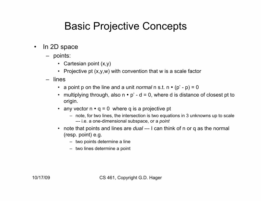
Basic Projective Concepts
• In 2D space – points:
• Cartesian point (x,y) • Projective pt (x,y,w) with convention that w is a scale factor
– lines • a point p on the line and a unit normal n s.t. n (p’ - p) = 0 • multiplying through, also n p’ - d = 0, where d is distance of closest pt to
origin. • any vector n q = 0 where q is a projective pt
– note, for two lines, the intersection is two equations in 3 unknowns up to scale --- i.e. a one-dimensional subspace, or a point
• note that points and lines are dual --- I can think of n or q as the normal (resp. point) e.g.
– two points determine a line – two lines determine a point

10/17/09 CS 461, Copyright G.D. Hager
Basic Projective Concepts
• In 3D space – points:
• Cartesian point (x,y,z) • Projective pt (x,y,z,w) with convention that w is a scale factor
– lines: • a point p on the line and unit vector v for direction
– for minimal parameterization, p is closest point to origin • Alternative, a line is the intersection of two planes (see below)
– planes • a point p on the plane and a unit normal n s.t. n (p’ - p) = 0 • multiplying through, also n p’ - d = 0, where d is distance of closest pt to
origin. • any vector n q = 0 where q is a projective pt
– note, for two planes, the intersection is two equations in 4 unknowns up to scale --- i.e. a one-dimensional subspace, or a line
• Note that planes and points are dual --- in the above, I can equally think of n or q as the normal (resp. point).

10/17/09 CS 461, Copyright G.D. Hager
Properties of SVD • Recall the Singular Value Decomposition of a matrix M (m by n) is
M = U D Vt where – U is m by n and has unit orthogonal columns (unitary) – D is n by n and has the singular values on the diagonal – V is n by n and has unit orthogonal columns (unitary)
• Interpretation: – V is the “input space” – D provides a “gain” for each input direction – U is a projection into the “output space”
• As a result: – The null space of M corresponds to the zero singular values in D – In most cases (e.g. Matlab) the singular values are sorted largest to smallest,
so the null space is the right-most columns of V – Matlab functions are
• [u,d,v] = SVD(m) • [u,d,v] = SVD(m,0) (“economy svd”)
– if m > n, only the first n singular values are computed and D is n by n – useful when solving overconstrained systems of equations

10/17/09 CS 461, Copyright G.D. Hager
Some Projective Concepts
• The vector p = (x,y,z,w)’ is equivalent to the vector k p for nonzero k – note the vector p = 0 is disallowed from this representation
• The vector v = (x,y,z,0)’ is termed a “point at infinity”; it corresponds to a direction
• In P2, – given two points p1 and p2, l = p1 x p2 is the line containing them – given two lines, l1, and l2, p = l1 x l2 is point of intersection – A point p lies on a line l if p l = 0 (note this is a consequence of the triple
product rule) – l = (0,0,1) is the “line at infinity” – it follows that, for any point p at infinity, l p = 0, which implies that points at
infinity lie on the line at infinity.

10/17/09 CS 461, Copyright G.D. Hager
Some Projective Concepts
• The vector p = (x,y,z,w)’ is equivalent to the vector k p for nonzero k – note the vector p = 0 is disallowed from this representation
• The vector v = (x,y,z,0)’ is termed a “point at infinity”; it corresponds to a direction
• In P3, – A point p lies on a plane l if p l = 0 (note this is a consequence of the triple
product rule; there is an equivalent expression in determinants) – l = (0,0,0,1) is the “plane at infinity” – it follows that, for any point p at infinity, l p = 0, which implies that points at
infinity lie on the line at infinity.

10/17/09 CS 461, Copyright G.D. Hager
Parallel lines meet
• First, show how lines project to images.
• Second, consider lines that have the same direction (are parallel) but are not parallel to the imaging plane
• Third, consider the degenerate case of lines parallel to the image plane – (by convention, the vanishing point is at infinity!)
A Good Exercise: Show this is the case!

10/17/09 CS 461, Copyright G.D. Hager
�������Compute the camera intrinsic (4 or more) and extrinsic parameters (6) using only observed
camera data.
Camera Calibration: Problem Statement

10/17/09 CS 461, Copyright G.D. Hager
Camera Calibration
• General strategy: – view calibration object – identify image points – obtain camera matrix by
minimizing error – obtain intrinsic parameters from
camera matrix
• Most modern systems employ the multi-plane method
– avoids knowing absolute coordinates of calibration poitns
• Error minimization: – Linear least squares
• easy problem numerically • solution can be rather bad
– Minimize image distance • more difficult numerical problem • solution usually rather good, but
can be hard to find – start with linear least squares
– Numerical scaling is an issue
Calibration = the computation of the camera intrinsic and extrinsic parameters

10/17/09 CS 461, Copyright G.D. Hager
A Quick Aside: Least Squares • Total least squares: a xi + b yi = zi
– Leads to mina,b ∑i (a xi + b yi - zi)2 – Equivalent to mind ∑i || dt ui - zi ||2 – Equivalent to minU || U d - z ||2 – Solution is given by taking derivatives yielding Ut U d = Ut z
• This implies that Ut U must be full rank!
• Suppose I have f(p, xi) = zi – minp ∑i || f(p, xi) - zi ||2 – Many solutions, however notice if we Taylor series expand f, we get – minΔp ∑i || f(p0, xi) + Jf(p0,xi) Δp - zi ||2 – Define “innovation” bi = f(p0,xi) - zi – Define J = [Jf(p0,x1); Jf(p0,x2) ...; Jf(p0,xn)] – Solve minM p || J Δp - b ||2
• This is now the same as the previous problem
• Finally, suppose we have A ui = bi and we are looking for A – minA ∑i || A ui - bi ||2 – Equivalent to minA || A U - B ||2F – Equivalent to solving A U = B in the least squares sense – Solution is to write A U Ut = B Ut ==> A = (U Ut)-1 B

Homogeneous systems
• Suppose I have ai u = 0 – minA || A u ||2
with A = [a1;a2; … an]
– Clearly u = 0 is a minimum, so add constraint ||u|| = 1 – Langrangian: minA,l || A u ||2 + l ||u -1||2 – Take gradient w.r.t u: AtA u + l u = 0 – Result --- u is eigenvector e of AtA – A e is eigenvalue; plugging into original optimization, choose
eigenvector with minimum eigenvalue – Done efficiently using SVD
10/17/09 CS 461, Copyright G.D. Hager

10/17/09 CS 461, Copyright G.D. Hager
Calibration: A Warmup
• Suppose we want to calibrate the affine camera and we know ui = A pi + d for many pairs i
• m is mean of u’s and q is mean of p’s; note m = A q + d
• U = [u1 - m,u2 - m, ... un-m] and P = [p1 - q,p2 -q, ... pn - q]
• U = A P U P’ (P P’)-1 = A
• d is now mean of ui – A pi

10/17/09 CS 461, Copyright G.D. Hager
Types of Calibration
• Photogrammetric Calibration • Self Calibration • Multi-Plane Calibration

10/17/09 CS 461, Copyright G.D. Hager
Photogrammetric Calibration
• Calibration is performed through imaging a pattern whose geometry in 3d is known with high precision.
• PRO: Calibration can be performed very efficiently • CON: Expensive set-up apparatus is required; multiple
orthogonal planes.
• Approach 1: Direct Parameter Calibration • Approach 2: Projection Matrix Estimation

10/17/09 CS 461, Copyright G.D. Hager
The General Case
• Affine is “easy” because it is linear and unconstrained (note orthographic is harder because of constraints)
• Perspective case is also harder because it is both nonlinear and constrained
• Observation: optical center can be computed from the orthocenter of vanishing points of orthogonal sets of lines.

Basic Equations
10/17/09 CS 461, Copyright G.D. Hager
€
u = (upix − cu) = sxu
v = (vpix − cv ) = syu
Known values

10/17/09 CS 461, Copyright G.D. Hager
Basic Equations
one of these for each point

10/17/09 CS 461, Copyright G.D. Hager
Basic Equations

10/17/09 CS 461, Copyright G.D. Hager
Basic Equations
We now know Rx and Ry up to a sign and γ. Rz = Rx x Ry
We will probably use another SVD to orthogonalize this system (R = U D V’; set D to I and multiply).

10/17/09 CS 461, Copyright G.D. Hager
Last Details
• We still need to compute the correct sign. – note that the denominator of the original equations must be positive
(points must be in front of the cameras) – Thus, the numerator and the projection must disagree in sign. – We know everything in numerator and we know the projection, hence
we can determine the sign.
• We still need to compute Tz and fx – we can formulate this as a least squares problem on those two
values using the first equation.

10/17/09 CS 461, Copyright G.D. Hager
Direct Calibration: The Algorithm
1. Compute image center from orthocenter 2. Compute the A matrix 3. Compute solution with SVD 4. Compute gamma and alpha 5. Compute R (and normalize) 6. Compute fx and and Tz
7. If necessary, solve a nonlinear regression to get distortion parameters

10/17/09 CS 461, Copyright G.D. Hager
Indirect Calibration: The Basic Idea
• We know that we can also just write – uh = M ph – x = (u/w) and y = (v/w), uh = (u,v,1)’ – As before, we can multiply through (after plugging in for u,v, and w)
• Once again, we can write – A m = 0
• Once again, we use an SVD to compute m up to a scale factor.
• We can again use algebra to recover the actual camera parameters from the matrix.

10/17/09 CS 461, Copyright G.D. Hager
Multi-Plane Calibration
• Hybrid method: Photogrammetric and Self-Calibration. • Uses a planar pattern imaged multiple times (inexpensive). • Used widely in practice and there are many implementations. • Based on a group of projective transformations called
homographies.
• Paper: Z. Zhang. – A flexible new technique for camera calibration. IEEE Transactions
on Pattern Analysis and Machine Intelligence, 22(11):1330-1334, 2000.
• Matlab implementation: – http://www.vision.caltech.edu/bouguetj/calib_doc/index.html

10/17/09 CS 461, Copyright G.D. Hager
Multi-Plane Calibration
• Hybrid method: Photogrammetric and Self-Calibration. • Uses a planar pattern imaged multiple times (inexpensive). • Used widely in practice and there are many implementations. • Based on a group of projective transformations called
homographies.
• m be a 2d point [u v 1]’ and M be a 3d point [x y z 1]’.
• Projection is

10/17/09 CS 461, Copyright G.D. Hager
Review: Projection Model
UVW
=
1 0 0 00 1 0 00 0 1
f 0
XYZT
UVW
pix
=
su 0 ou
0 sv ov
0 0 1
UVW
mm
= Ap
UVW
=
f 0 0 00 f 0 00 0 1 0
XYZT
UVW
pix
=
fsu 0 ou
0 fsv ov
0 0 1
UVW
mm
=
α γ u0
0 β v0
0 0 1
UVW
Ap

10/17/09 CS 461, Copyright G.D. Hager
Result
• Recall A = [r1 r2 t]
• Given matching point pairs, we can compute an homography H
• We know that
• From one homography, how many constraints on the intrinsic parameters can we obtain? – Extrinsics have 6 degrees of freedom. – The homography supplies 8 values. – Thus, we should be able to obtain 2 constraints per homography.
• Use the constraints on the rotation matrix columns…

10/17/09 CS 461, Copyright G.D. Hager
Computing Intrinsics
• Rotation Matrix is orthogonal….
• Write the homography in terms of its columns…

10/17/09 CS 461, Copyright G.D. Hager
Computing Intrinsics
• Derive the two constraints:

10/17/09 CS 461, Copyright G.D. Hager
Closed-Form Solution
• Notice B is symmetric, 6 parameters can be written as a vector b. • From the two constraints, we have h1
T B h2 = v12 b
• Stack up n of these for n images and build a 2n*6 system. • Solve with SVD. • Intrinsic parameters “fall-out” of the result easily using algebra

10/17/09 CS 461, Copyright G.D. Hager
Computing Extrinsics
First, compute H’ = A-1 H Note that first two columns of H’ should be rotation
use this to determine scaling factor Orthogonalize using SVD to get rotation Pull out translation as scaled last column

10/17/09 CS 461, Copyright G.D. Hager
Non-linear Refinement
• Closed-form solution minimized algebraic distance. • Since full-perspective is a non-linear model
– Can include distortion parameters (radial, tangential) – Use maximum likelihood inference for our estimated parameters.

10/17/09 CS 461, Copyright G.D. Hager
Multi-Plane Approach In Action
• …if we can get matlab to work…

10/17/09 CS 461, Copyright G.D. Hager
Camera parameters • Summary:
– points expressed in external frame – points are converted to canonical camera coordinates – points are projected – points are converted to pixel units
=
TZYX
WVU
parameters extrinsicngrepresenti
tionTransforma
model projectionngrepresenti
tionTransforma
parameters intrinsic ngrepresenti
tionTransforma
point in cam. coords.
point in metric image coords.
point in pixel coords. point in
world coords.

10/17/09 CS 461, Copyright G.D. Hager
Calibration Summary
• Two groups of parameters: – internal (intrinsic) and external (extrinsic)
• Many methods – direct and indirect, flexible/robust
• The form of the equations that arise here and the way they are solved is common in vision: – bilinear forms – Ax = 0 – Orthogonality constraints in rotations
• Most modern systems use the method of multiple planes (matlab demo) – more difficult optimization over a large # of parameters – more convenient for the user

10/17/09 CS 461, Copyright G.D. Hager
Lens Distortion
• In general, lens introduce minor irregularities into images, typically radial distortions:
x = xd(1 + k1r2 + k2r4) y = yd(1 + k1r2 + k2r4) r2 = xd
2 + yd2
• The values k1 and k2 are additional parameters that must be estimated in order to have a model for the camera system.
– The complete model is then: q = distort(k1,k2, K(sx, sy, ox, oy) * (Π(p; R, t)))

The Final Iterations
• Recall scalar linear least squares: – minx sumi (y – a x)2
• To go to multiple dimensions
– minx sumi ||y – A x||2
• What if we have a nonlinear problem?
• minx sumi ||y – F(x)||2
10/17/09 CS 461, Copyright G.D. Hager

Multi-Camera Calibration
• Note that I might observe a target simultaneously in two or more cameras – For any given pair, I can solve for the transformation between them – For multiple pairs, I can optimize the relative location
• This is the natural lead-in to computational stereo …
10/17/09 CS 461, Copyright G.D. Hager

10/17/09 CS 461, Copyright G.D. Hager
Resampling Using Homographies
• Pick a rotation matrix R from old to new image
• Consider all points in the image you want to compute; then – construct pixel coordinates x = (u,v,1) – K maps unit focal length metric coordinates to pixel (normalized
camera) – x’ = K Rt K-1 x x’ = H x
• Sample a point x’ in the original image for each point x in the new.
pixel coordinates pixel coordinates
pixel to euclidean coords euclidean to pixel coords
rotation

10/17/09 CS 461, Copyright G.D. Hager
Rectification
• The goal of rectification is to turn a verged camera system into a non-verged system. – Let us assume we know pr = rRl pl + T
• how would we get this out of camera calibration?
• Observation: – consider a coordinate system where the stereo baseline defines the
x axis, z is any axis orthogonal to it, and y is z cross x. • x = T/||T|| • y = ([0,0,1] £ x )/|| [0,0,1] £ x || • z = x cross y
– Note that both the left and right camera can now be rotated to be parallel to this frame
• lRu = [x y z] is the rotation from unverged to verged frame for left camera • rRu = rRl
lRu

10/17/09 CS 461, Copyright G.D. Hager
Bilinear Interpolation
• A minor detail --- new value x’ = (u’,v’,1) may not be integer
• let u’ = i + fu and v’ = j+fv
• New image value b = (1-fu)((1-fv)I(j,i) + fv I(j+1,i)) + fu((1-fv)I(j,i+1) + fv I(j+1,i+1))

Estimating Changes of Coordinates
• Affine Model: y = A x + d
• How do we solve this given matching pairs of y’s and x’s?
• How many points do we need for a unique solution?
• Note this can be written sum_i || y – Ax –d ||2 – It can also be written using the Frobenius norm
• Answer:
10/17/09 CS 461, Copyright G.D. Hager

Estimating Changes of Coordinates
• Consider a 2D Euclidean model – y = R x + t
• How many points to solve for this transformation?
• Consider a 3D Euclidean model – y= R x + t
• How many points to solve for this transformation?
• Here, SVD will come to the rescue! – Compute barycentric y’ and x’ – Compute M = Y’ X’T
– M = U D VT – R = V UT
10/17/09 CS 461, Copyright G.D. Hager

10/17/09 CS 461, Copyright G.D. Hager
An Approximation: The Affine Camera
• Choose a nominal point x0, y0, z0 and describe projection relative to that point
• u = f [x0/z0 + (x-x0)/z0 - x0/z20 (z – z0) ] = f (a1 x + a2 z + d1)
• v = f [y0/z0 + (y – y0)/z0 – y0/z20 (z – z0) = f (a3 y + a4 z + d2)
• gathering up
• A = [a1 0 a2; 0 a3 a4] • d = [d1; d2]
• u = A P + d
• add external transform
• u = A (RP + T) + d --> u = A* Q where A* is 2x4 rank 2 Matrix and Q is homogeneous version of P
=
TZYX
fdaadaa
WVU
/10000
0
243
121
alternatively:
alternatively:

10/17/09 CS 461, Copyright G.D. Hager
Summary: Other Models
• The orthographic and scaled orthographic cameras (also called weak perspective)
– simply ignore z – differ in the scaling from x/y to u/v coordinates – preserve Euclidean structure to a great degree
• The affine camera is a generalization of orthographic models. – u = A p + d – A is 2 x 3 and d is 2x1 – This can be derived from scaled orthography or by linearizing perspective
about a point not on the optical axis
• The projective camera is a generalization of the perspective camera. – u’ = M p – M is 3x4 nonsingular defined up to a scale factor – This just a generalization (by one parameter) from “real” model
• Both have the advantage of being linear models on real and projective spaces, respectively.

10/17/09 CS 461, Copyright G.D. Hager
Model Stratification Euclidean Similarity Affine Projective
Transforms rotation x x x x translation x x x x uniform scaling x x x nonuniform scaling x x shear x x perspective x composition of proj. x Invariants length x angle x x ratios x x parallelism x x x incidence/cross rat. x x x x

10/17/09 CS 461, Copyright G.D. Hager
Why Projective (or Affine or ...) • Recall in Euclidean space, we can define a change of coordinates by choosing a new origin
and three orthogonal unit vectors that are the new coordinate axes – The class of all such transformation is SE(3) which forms a group – One rendering is the class of all homogeneous transformations – This does not model what happens when things are imaged (why?)
• If we allow a change in scale, we arrive at similarity transforms, also a group – This sometimes can model what happens in imaging (when?)
• If we allow the 3x3 rotation to be an arbitrary member of GL(3) we arrive at affine transformations (yet another group!)
– This also sometimes is a good model of imaging – The basis is now defined by three arbitrary, non-parallel vectors
• The process of perspective projection does not form a group – that is, a picture of a picture cannot in general be described as a perspective projection
• Projective systems include perspectivities as a special case and do form a group – We now require 4 basis vectors (three axes plus an additional independent vector) – A model for linear transformations (also called collineations or homographies) on Pn is GL(n+1) which
is, of course, a group

10/17/09 CS 461, Copyright G.D. Hager
Basic Equations

10/17/09 CS 461, Copyright G.D. Hager
A Quick Aside: Least Squares • Familiar territory is yi = a xi + b ==> mina,b ∑i (a xi + b - yi)
• Total least squares: a xi + b yi = zi – Leads to mina,b ∑i (a xi + b yi - zi)2 – Equivalent to mind ∑i || dt ui - zi ||2 – Equivalent to minU || U d - z ||2 – Solution is given by taking derivatives yielding Ut U d = Ut z
• This implies that Ut U must be full rank!
• Another way to think of this: – let d = (a, b, 1) – Let wi = (xi,yi,zi), W the matrix with rows wi – Then we can write
• mind || Wd ||2F with ||d|| = 1 or Wt W d = 0 with ||d|| = 1 • Another way to state this is solve W d = 0 in least squares sense with ||d|| = 1 • How do we solve this?