Computer vision

CC1002 - Computer Vision

using HPC

Dr. C. Saravanan

NIT Durgapur

[email protected]

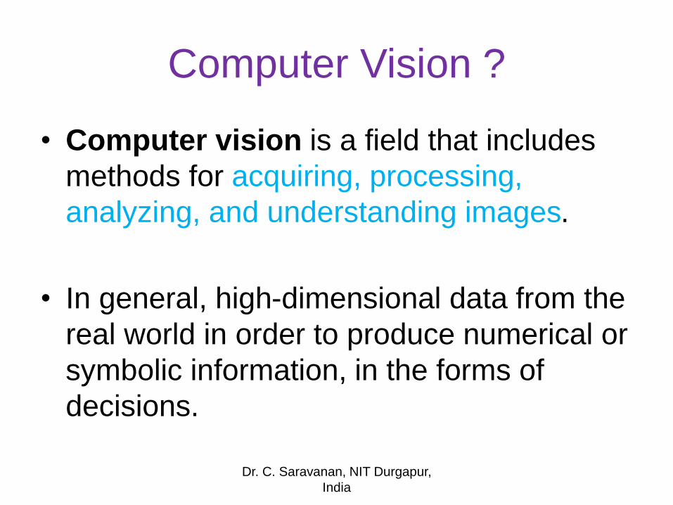
Computer Vision ?

• Computer vision is a field that includes

methods for acquiring, processing,

analyzing, and understanding images.

• In general, high-dimensional data from the

real world in order to produce numerical or

symbolic information, in the forms of

decisions.

Dr. C. Saravanan, NIT Durgapur,

India

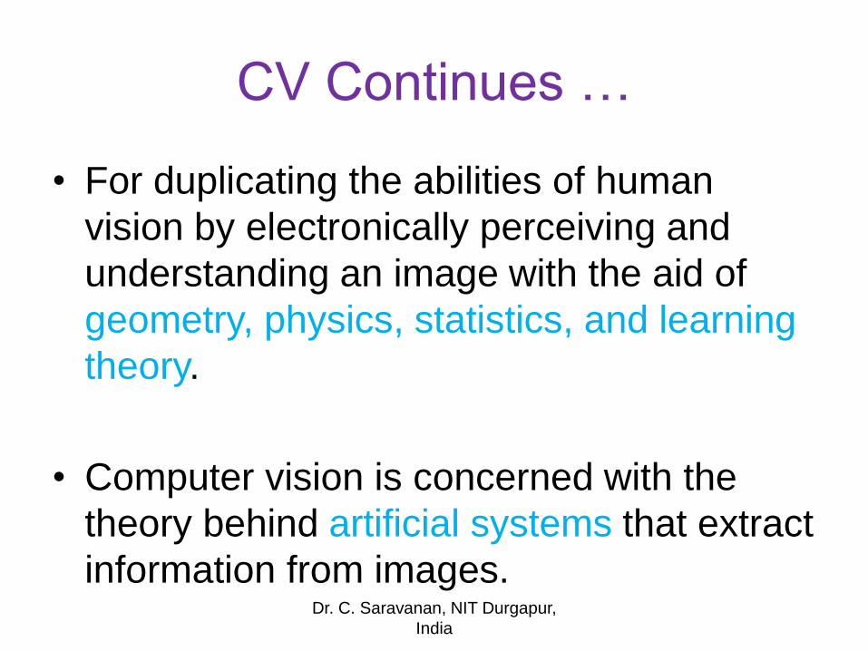
CV Continues …

• For duplicating the abilities of human

vision by electronically perceiving and

understanding an image with the aid of

geometry, physics, statistics, and learning

theory.

• Computer vision is concerned with the

theory behind artificial systems that extract

information from images. Dr. C. Saravanan, NIT Durgapur,

India

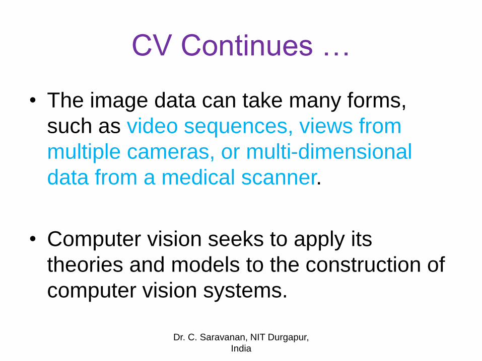
CV Continues …

• The image data can take many forms,

such as video sequences, views from

multiple cameras, or multi-dimensional

data from a medical scanner.

• Computer vision seeks to apply its

theories and models to the construction of

computer vision systems.


India

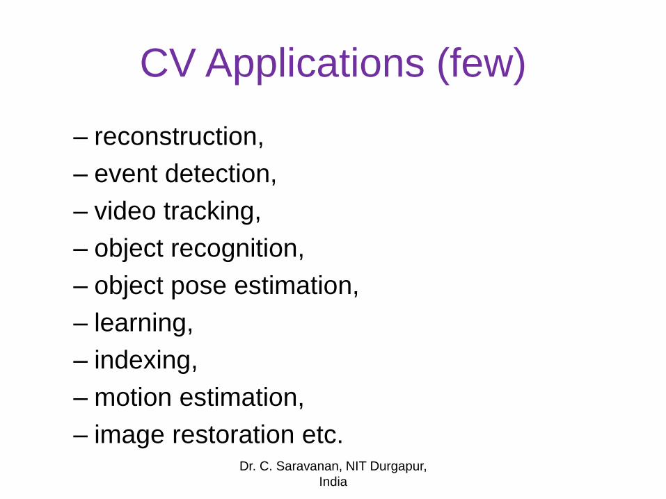
CV Applications (few)

– reconstruction,

– event detection,

– video tracking,

– object recognition,

– object pose estimation,

– learning,

– indexing,

– motion estimation,

– image restoration etc.Dr. C. Saravanan, NIT Durgapur,

India

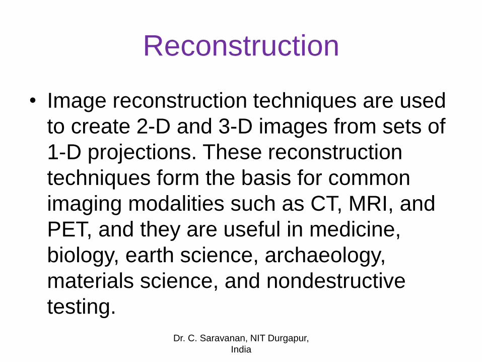
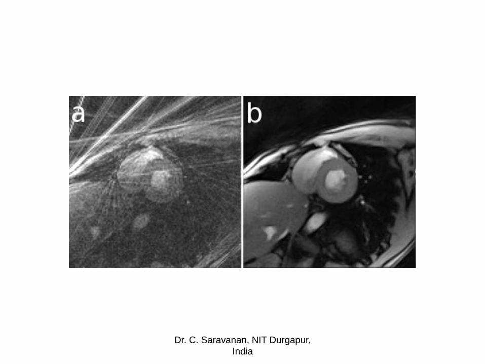
Reconstruction

• Image reconstruction techniques are used

to create 2-D and 3-D images from sets of

1-D projections. These reconstruction

techniques form the basis for common

imaging modalities such as CT, MRI, and

PET, and they are useful in medicine,

biology, earth science, archaeology,

materials science, and nondestructive

testing.


India


India

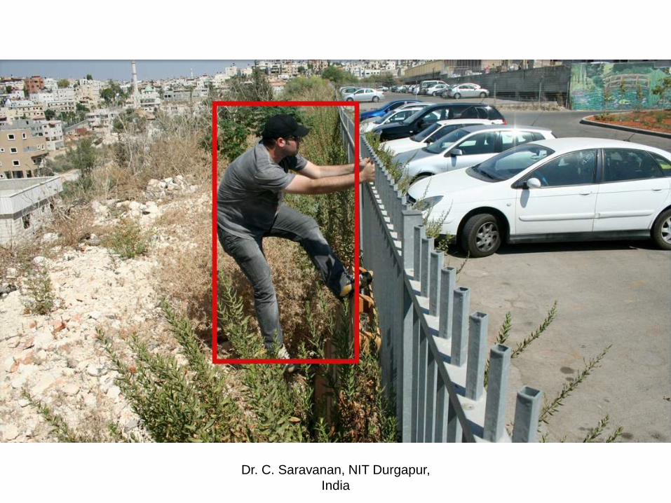
Event Detection

• An interesting event may be defined as

something that is “not normal”.

• For this purpose, we need to model the

normal situation and device means to

discover deviations from this model.


India


India

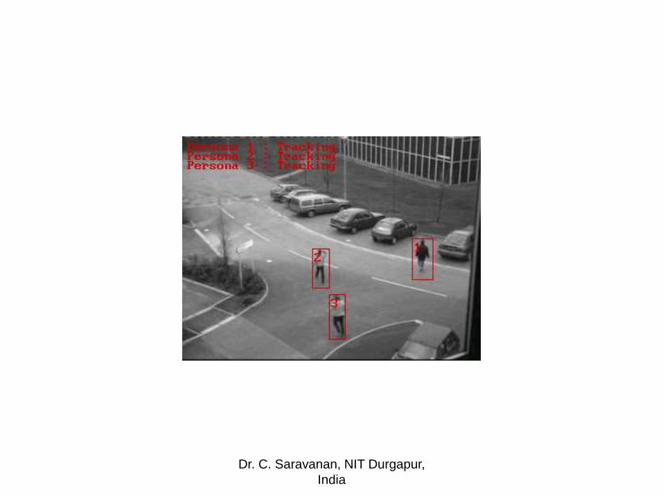
Video Tracking

• Video tracking is the process of locating

a moving object (or multiple objects) over

time using a camera. It has a variety of

uses, some of which are: human-computer

interaction, security and surveillance,

video communication and compression,

augmented reality, traffic control, medical

imaging and video editing.


India

https://en.wikipedia.org/wiki/Motion_(physics)

https://en.wikipedia.org/wiki/Video_compression

Video Tracking

• Video tracking can be a time consuming

process due to the amount of data that is

contained in video. Adding further to the

complexity is the possible need to

use object recognition techniques for

tracking, a challenging problem in its own

right.


India

https://en.wikipedia.org/wiki/Object_recognition


India

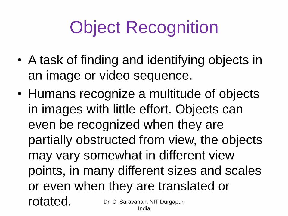
Object Recognition

• A task of finding and identifying objects in

an image or video sequence.

• Humans recognize a multitude of objects

in images with little effort. Objects can

even be recognized when they are

partially obstructed from view, the objects

may vary somewhat in different view

points, in many different sizes and scales

or even when they are translated or

rotated. Dr. C. Saravanan, NIT Durgapur,

India


India

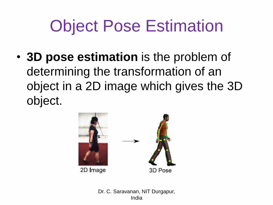
Object Pose Estimation

• 3D pose estimation is the problem of

determining the transformation of an

object in a 2D image which gives the 3D

object.


India


India

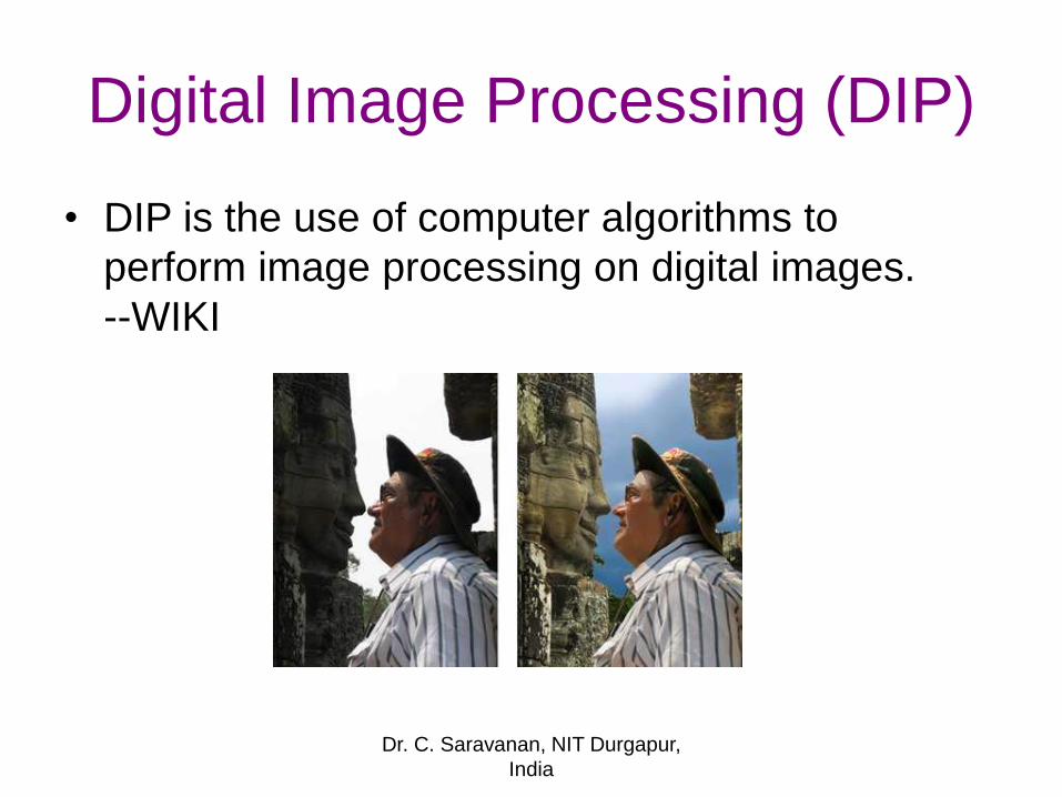
Digital Image Processing (DIP)

• DIP is the use of computer algorithms to

perform image processing on digital images.

--WIKI


India

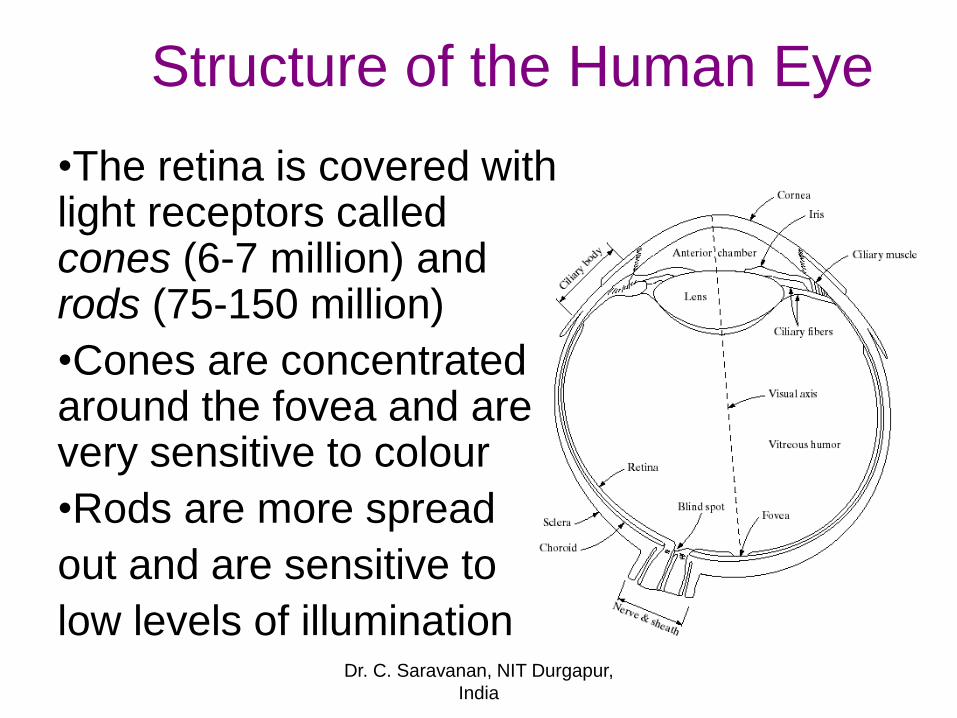
Structure of the Human Eye

•The retina is covered with light receptors called cones (6-7 million) androds (75-150 million)

•Cones are concentrated around the fovea and are very sensitive to colour

•Rods are more spread

out and are sensitive to

low levels of illuminationDr. C. Saravanan, NIT Durgapur,

India

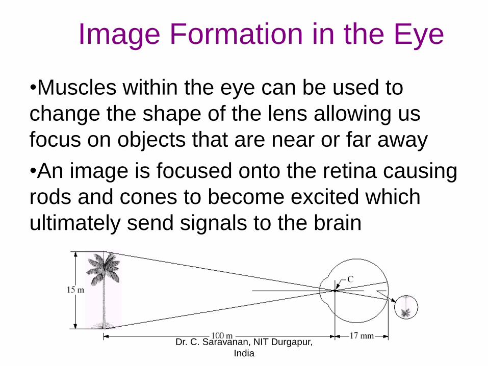
Image Formation in the Eye

•Muscles within the eye can be used to

change the shape of the lens allowing us

focus on objects that are near or far away

•An image is focused onto the retina causing

rods and cones to become excited which

ultimately send signals to the brain


India

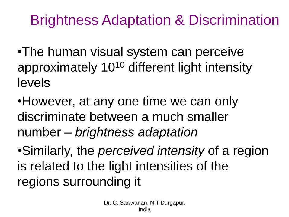
Brightness Adaptation & Discrimination

•The human visual system can perceive

approximately 1010 different light intensity

levels

•However, at any one time we can only

discriminate between a much smaller

number – brightness adaptation

•Similarly, the perceived intensity of a region

is related to the light intensities of the

regions surrounding it


India

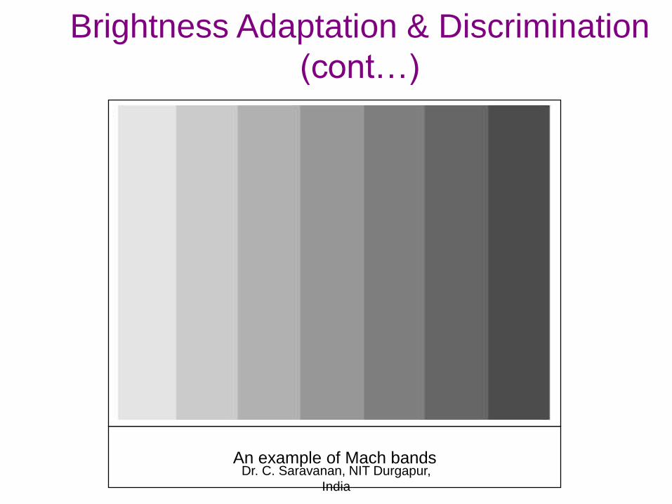
Brightness Adaptation & Discrimination

(cont…)

An example of Mach bandsDr. C. Saravanan, NIT Durgapur,

India

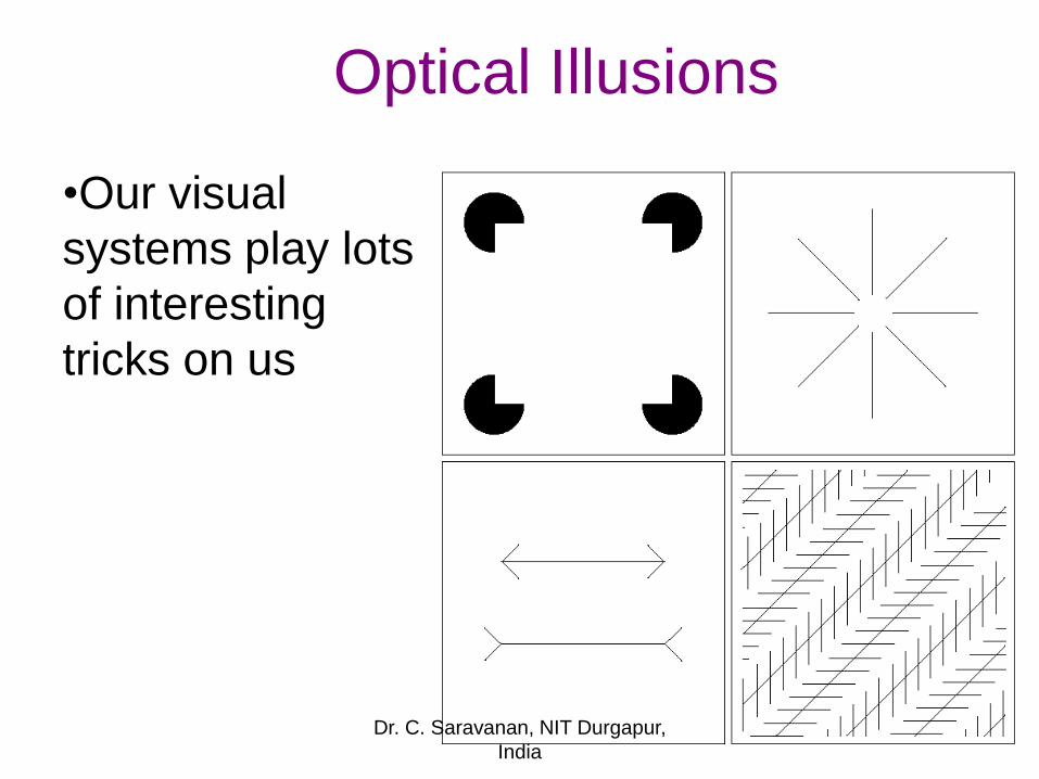
Optical Illusions

•Our visual

systems play lots

of interesting

tricks on us


India

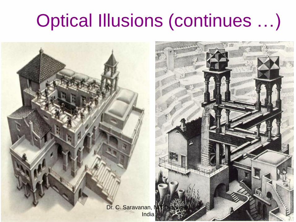
Optical Illusions (continues …)


India

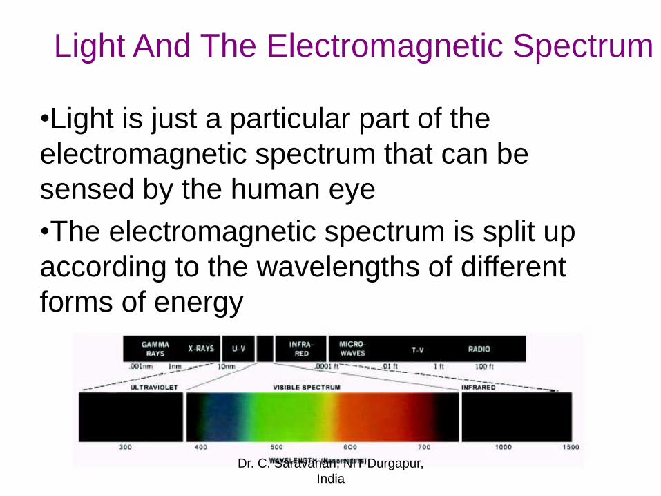
Light And The Electromagnetic Spectrum

•Light is just a particular part of the

electromagnetic spectrum that can be

sensed by the human eye

•The electromagnetic spectrum is split up

according to the wavelengths of different

forms of energy


India

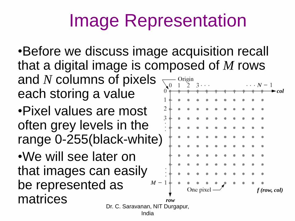
Image Representation

col

row

f (row, col)

•Before we discuss image acquisition recall that a digital image is composed of M rows and N columns of pixels each storing a value

•Pixel values are most often grey levels in the range 0-255(black-white)

•We will see later on that images can easily be represented as matrices


India

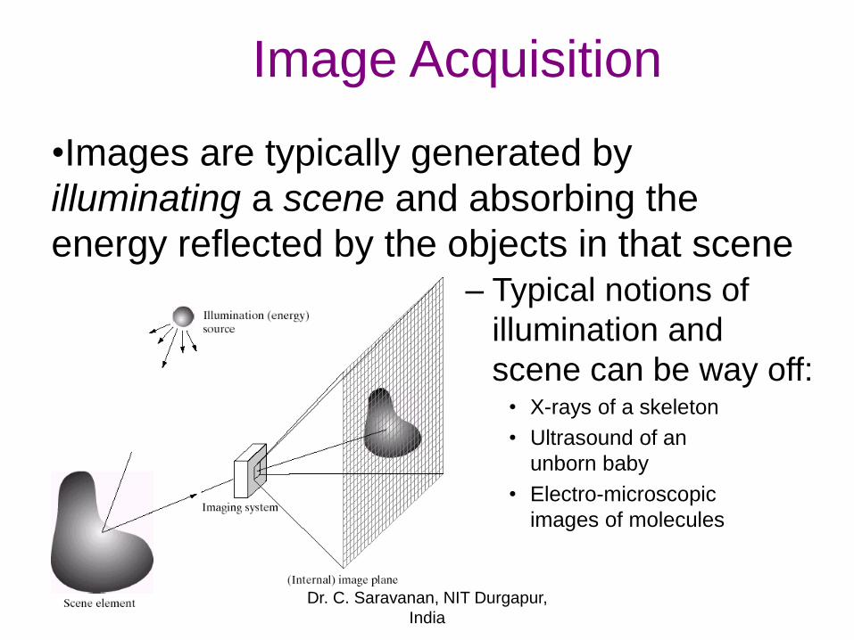
Image Acquisition

•Images are typically generated by

illuminating a scene and absorbing the

energy reflected by the objects in that scene– Typical notions of

illumination and

scene can be way off:• X-rays of a skeleton

• Ultrasound of an

unborn baby

• Electro-microscopic

images of molecules


India

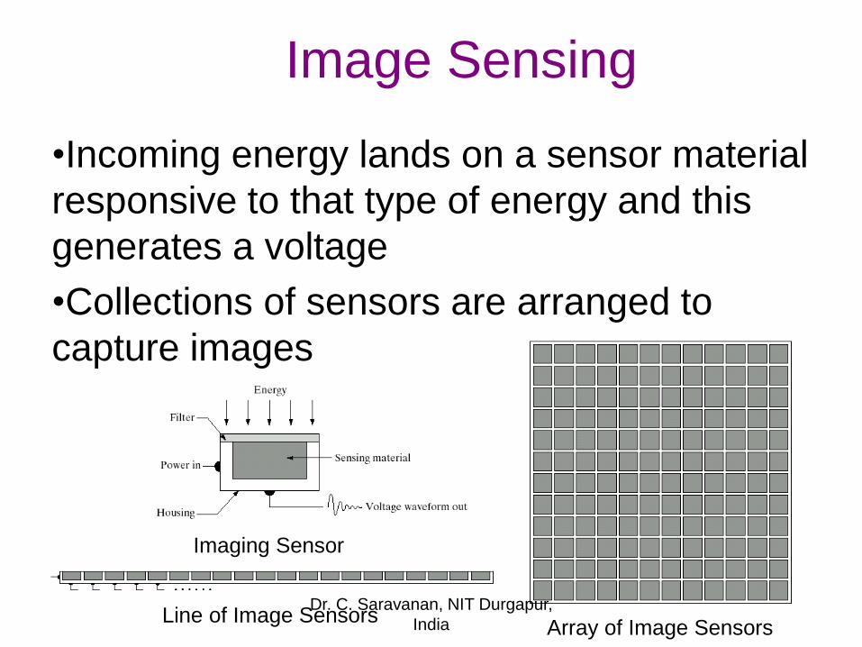
Image Sensing

•Incoming energy lands on a sensor material

responsive to that type of energy and this

generates a voltage

•Collections of sensors are arranged to

capture images

Imaging Sensor

Line of Image SensorsArray of Image Sensors


India

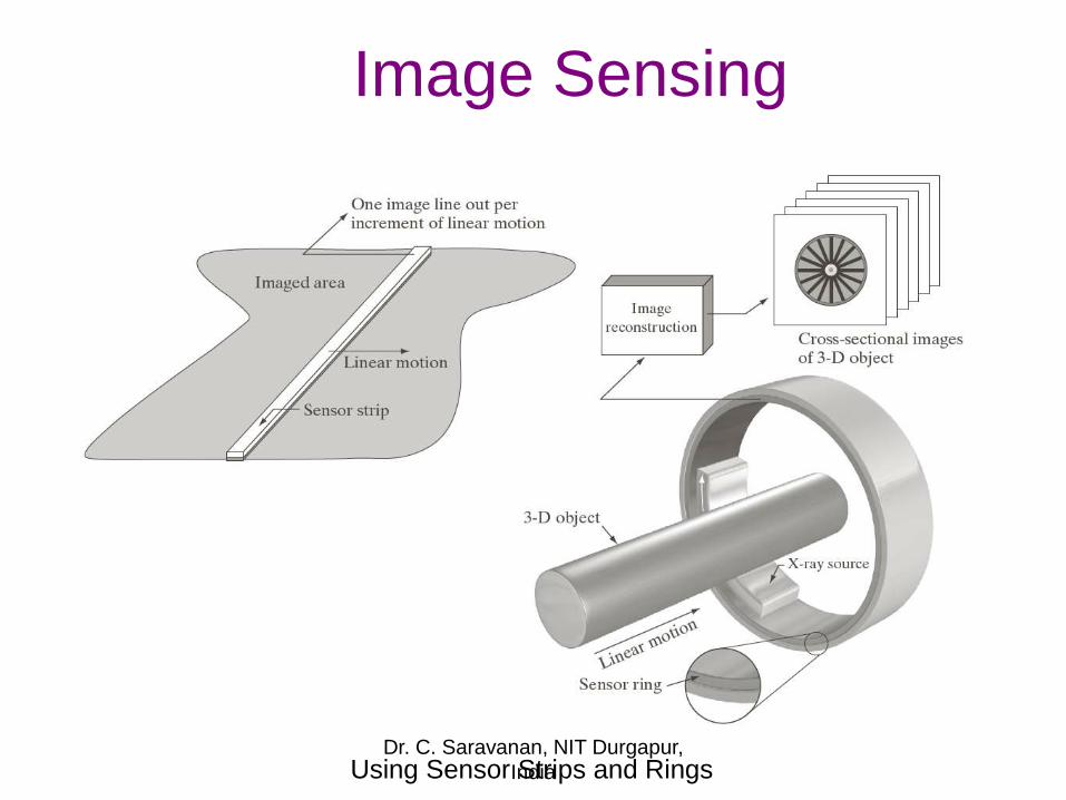
Image Sensing

Using Sensor Strips and RingsDr. C. Saravanan, NIT Durgapur,

India

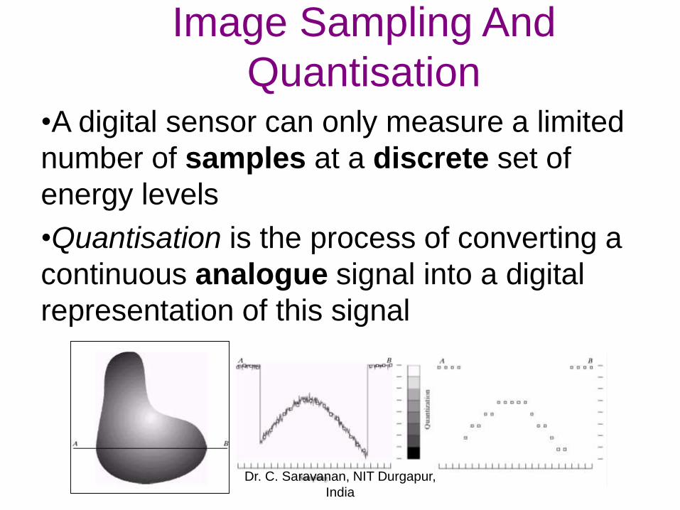
Image Sampling And

Quantisation•A digital sensor can only measure a limited

number of samples at a discrete set of

energy levels

•Quantisation is the process of converting a

continuous analogue signal into a digital

representation of this signal


India

Image Sampling And Quantisation

(continues …)

•Remember that a digital image is always

only an approximation of a real world

scene


India

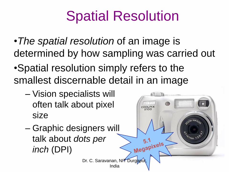
Spatial Resolution

•The spatial resolution of an image is

determined by how sampling was carried out

•Spatial resolution simply refers to the

smallest discernable detail in an image

– Vision specialists will

often talk about pixel

size

– Graphic designers will

talk about dots per

inch (DPI)Dr. C. Saravanan, NIT Durgapur,

India

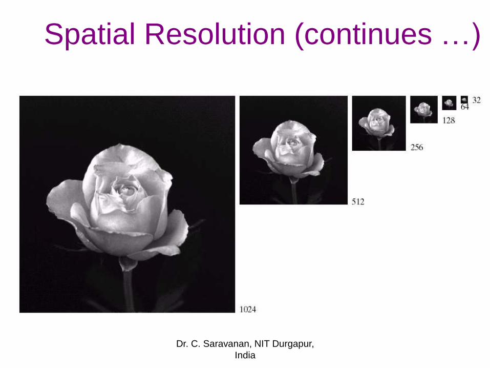
Spatial Resolution (continues …)


India

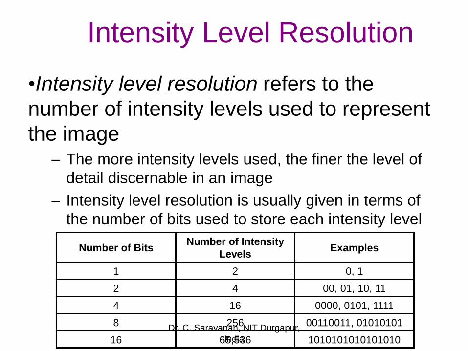
Intensity Level Resolution

•Intensity level resolution refers to the

number of intensity levels used to represent

the image– The more intensity levels used, the finer the level of

detail discernable in an image

– Intensity level resolution is usually given in terms of

the number of bits used to store each intensity level

Number of BitsNumber of Intensity

LevelsExamples

1 2 0, 1

2 4 00, 01, 10, 11

4 16 0000, 0101, 1111

8 256 00110011, 01010101

16 65,536 1010101010101010


India

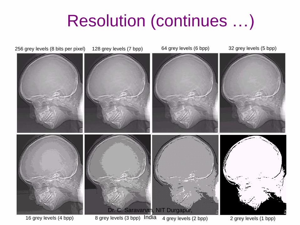
Resolution (continues …)

128 grey levels (7 bpp) 64 grey levels (6 bpp) 32 grey levels (5 bpp)

16 grey levels (4 bpp) 8 grey levels (3 bpp) 4 grey levels (2 bpp) 2 grey levels (1 bpp)

256 grey levels (8 bits per pixel)


India

Resolution: How Much Is

Enough?•The big question with resolution is always

how much is enough?

– This all depends on what is in the image and

what you would like to do with it

– Key questions include

• Does the image look aesthetically pleasing?

• Can you see what you need to see within the

image?


India

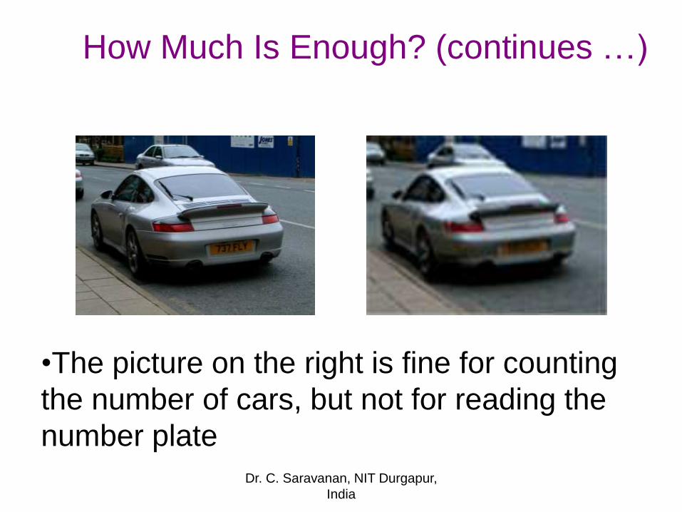
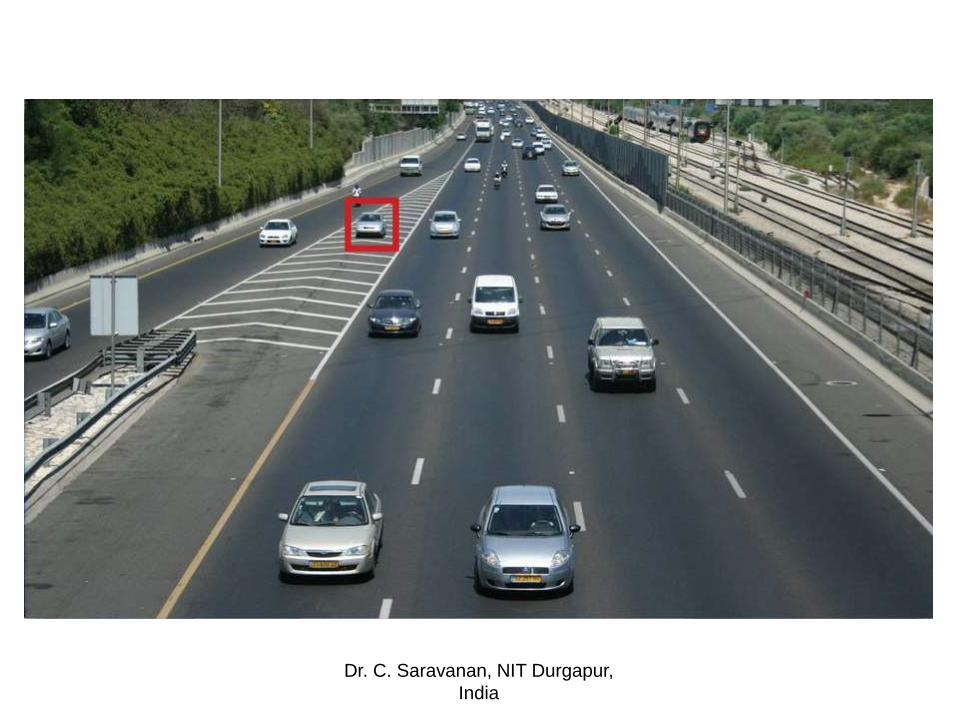
How Much Is Enough? (continues …)

•The picture on the right is fine for counting

the number of cars, but not for reading the

number plate


India

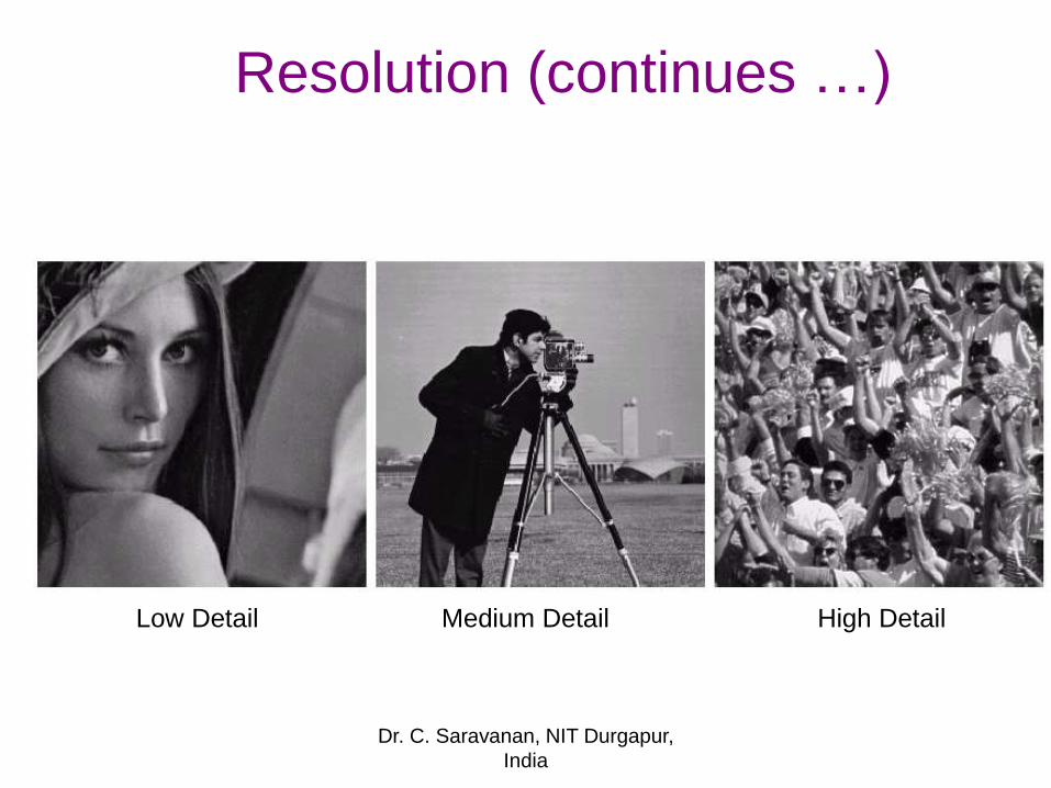
Resolution (continues …)

Low Detail Medium Detail High Detail


India

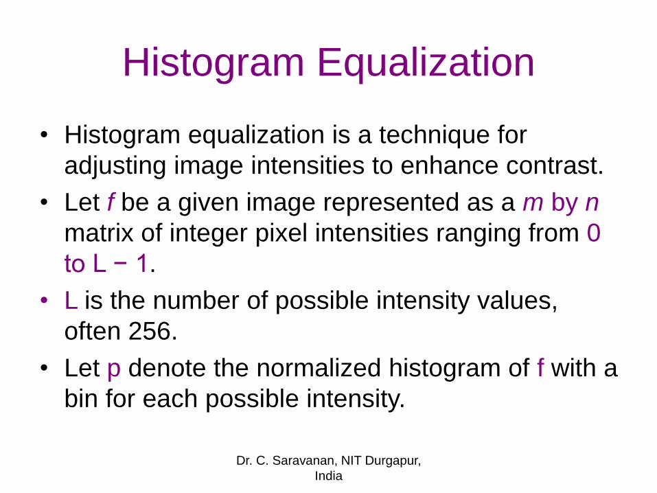
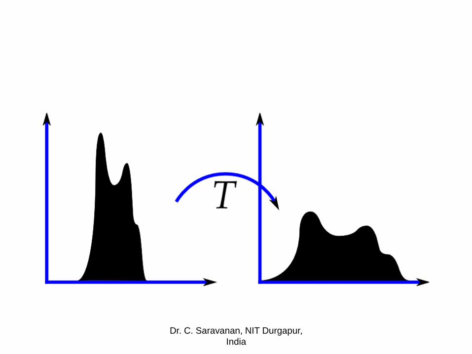
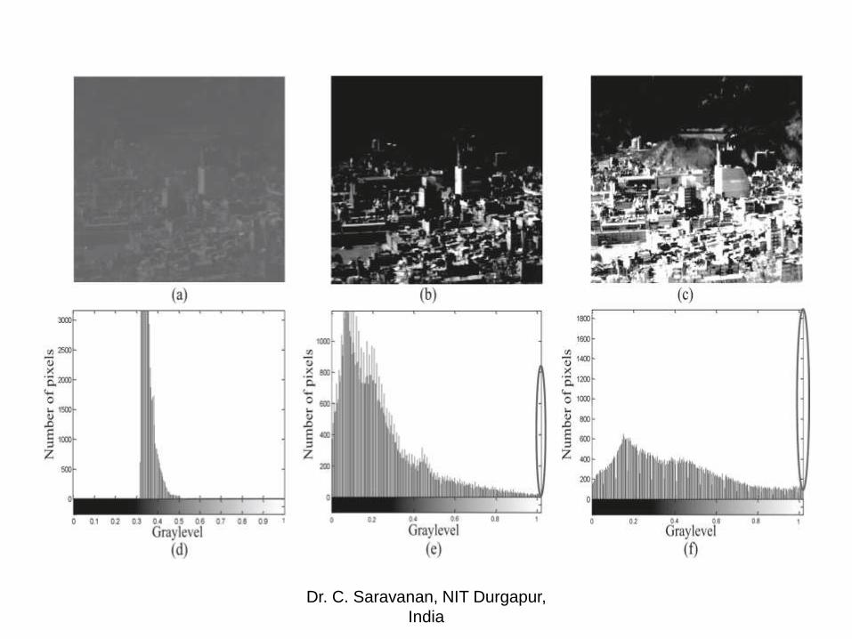
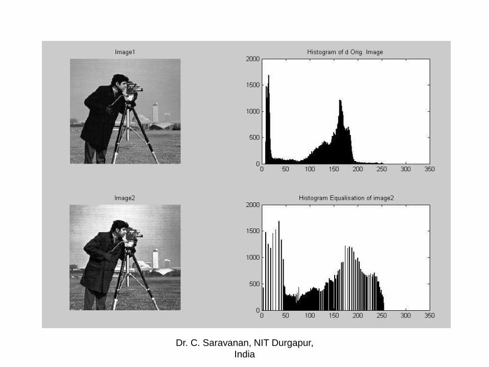
Histogram Equalization

• Histogram equalization is a technique for

adjusting image intensities to enhance contrast.

• Let f be a given image represented as a m by n

matrix of integer pixel intensities ranging from 0

to L − 1.

• L is the number of possible intensity values,

often 256.

• Let p denote the normalized histogram of f with a

bin for each possible intensity.


India

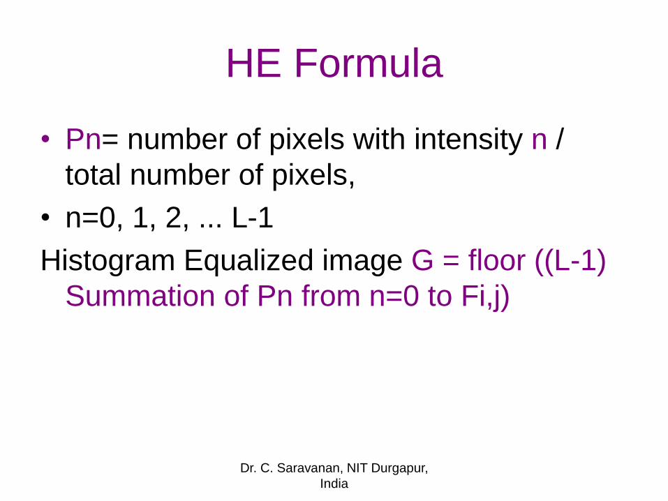
HE Formula

• Pn= number of pixels with intensity n /

total number of pixels,

• n=0, 1, 2, ... L-1

Histogram Equalized image G = floor ((L-1)

Summation of Pn from n=0 to Fi,j)


India


India

Correlation and Convolution

• Correlation and Convolution are basic operations that we will perform to extract information from images.

• They are shift-invariant, and they are linear.

• Shift-invariant means that we perform the same operation at every point in the image.

• Linear means that we replace every pixel with a linear combination of its neighbors.


India

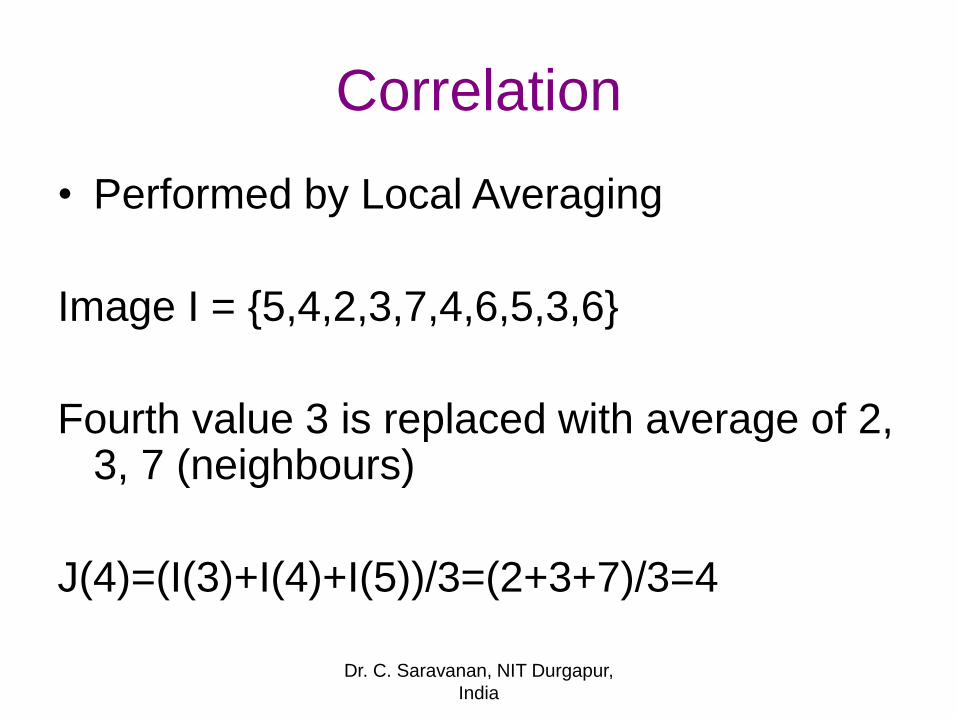
Correlation

• Performed by Local Averaging

Image I = {5,4,2,3,7,4,6,5,3,6}

Fourth value 3 is replaced with average of 2, 3, 7 (neighbours)

J(4)=(I(3)+I(4)+I(5))/3=(2+3+7)/3=4


India

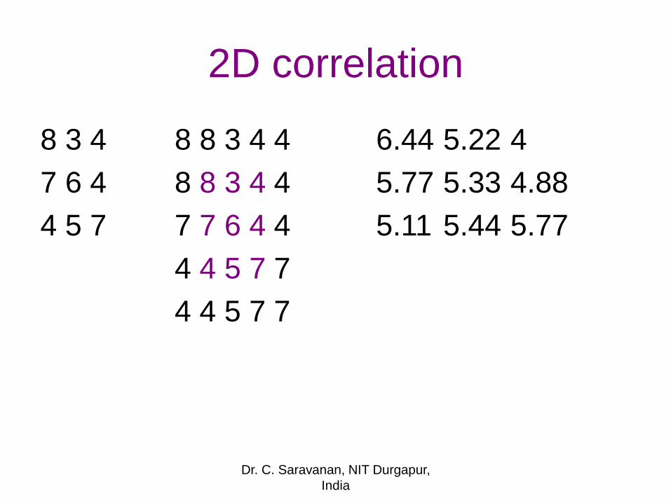
2D correlation

8 3 4 8 8 3 4 4 6.44 5.22 4

7 6 4 8 8 3 4 4 5.77 5.33 4.88

4 5 7 7 7 6 4 4 5.11 5.44 5.77

4 4 5 7 7

4 4 5 7 7


India

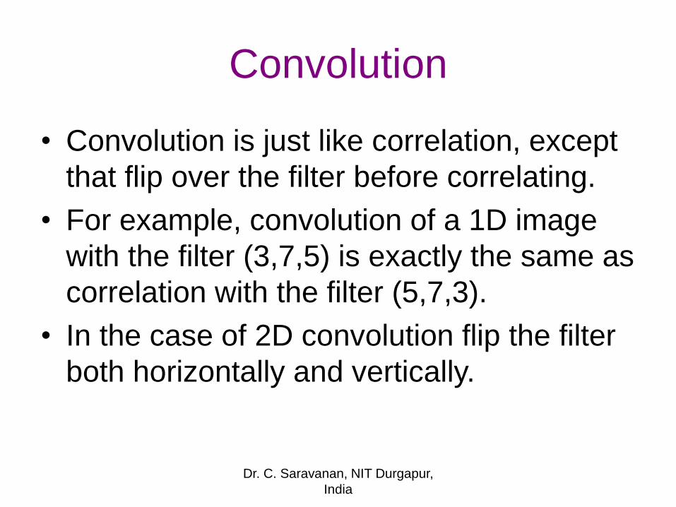
Convolution

• Convolution is just like correlation, except

that flip over the filter before correlating.

• For example, convolution of a 1D image

with the filter (3,7,5) is exactly the same as

correlation with the filter (5,7,3).

• In the case of 2D convolution flip the filter

both horizontally and vertically.


India

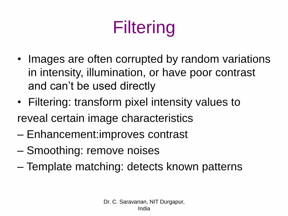
Filtering

• Images are often corrupted by random variations

in intensity, illumination, or have poor contrast

and can’t be used directly

• Filtering: transform pixel intensity values to

reveal certain image characteristics

– Enhancement:improves contrast

– Smoothing: remove noises

– Template matching: detects known patterns


India

Smoothing Filters

• Additive smoothing / Laplace / Lidstone

• Butterworth filter

• Digital filter

• Kalman filter

• Kernel smoother

• Laplacian smoothing

• Stretched grid method

• Low-pass filter

• Savitzky–Golay smoothing filter based on the least-squares fitting of polynomials

• Local regression also known as "loess" or "lowess"

• Smoothing spline

• Ramer–Douglas–Peucker algorithm

• Moving average

• Exponential smoothing

• Kolmogorov–Zurbenko filter


India

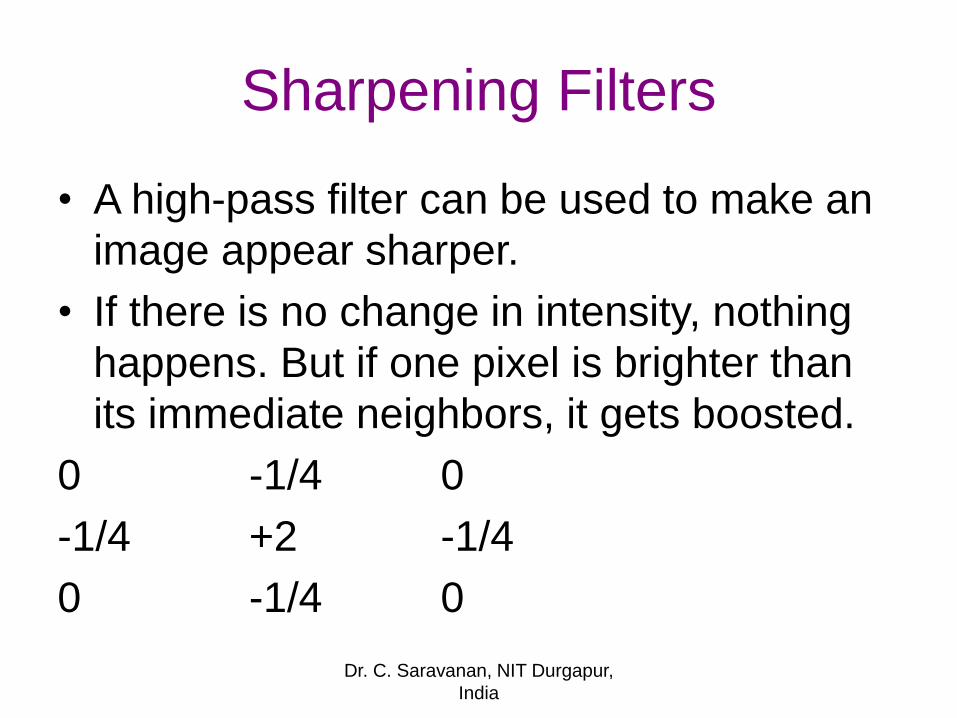
Sharpening Filters

• A high-pass filter can be used to make an

image appear sharper.

• If there is no change in intensity, nothing

happens. But if one pixel is brighter than

its immediate neighbors, it gets boosted.

0 -1/4 0

-1/4 +2 -1/4

0 -1/4 0


India

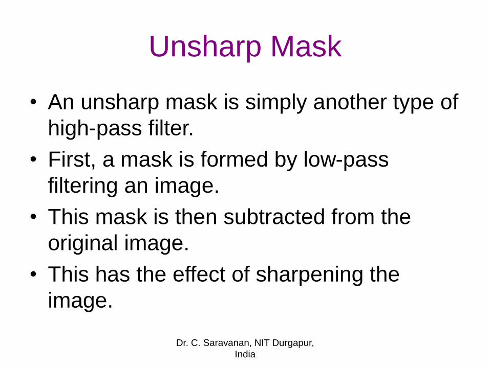
Unsharp Mask

• An unsharp mask is simply another type of

high-pass filter.

• First, a mask is formed by low-pass

filtering an image.

• This mask is then subtracted from the

original image.

• This has the effect of sharpening the

image.


India

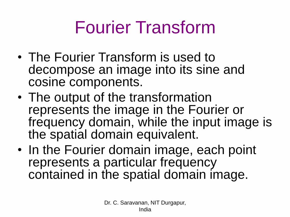
Fourier Transform

• The Fourier Transform is used to decompose an image into its sine and cosine components.

• The output of the transformation represents the image in the Fourier or frequency domain, while the input image is the spatial domain equivalent.

• In the Fourier domain image, each point represents a particular frequency contained in the spatial domain image.


India

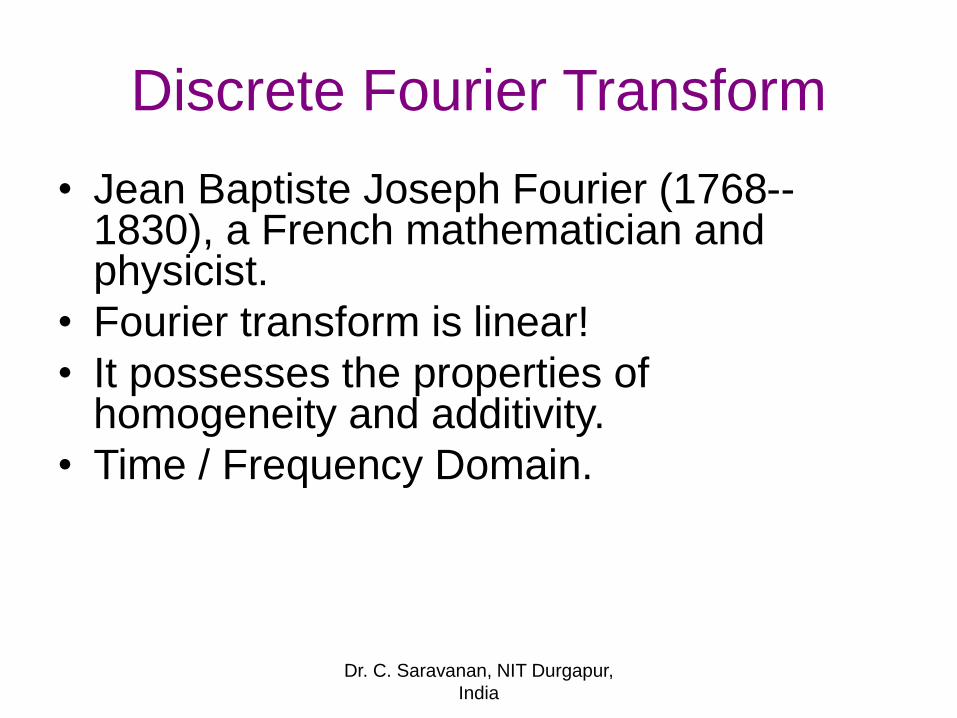
Discrete Fourier Transform

• Jean Baptiste Joseph Fourier (1768--1830), a French mathematician and physicist.

• Fourier transform is linear!

• It possesses the properties ofhomogeneity and additivity.

• Time / Frequency Domain.


India

DFT

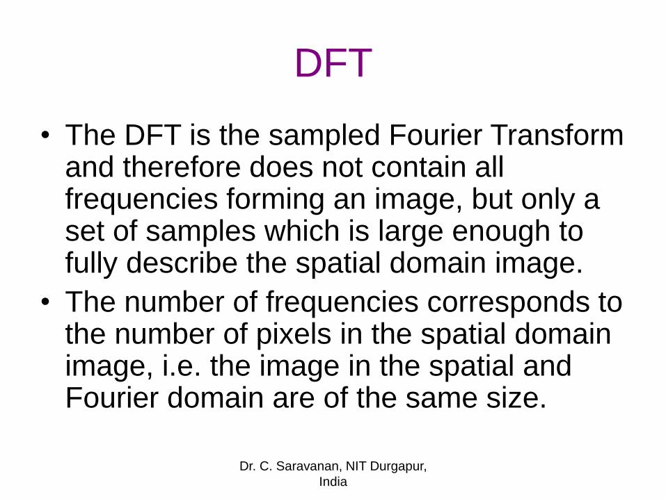
• The DFT is the sampled Fourier Transform and therefore does not contain all frequencies forming an image, but only a set of samples which is large enough to fully describe the spatial domain image.

• The number of frequencies corresponds to the number of pixels in the spatial domain image, i.e. the image in the spatial and Fourier domain are of the same size.


India

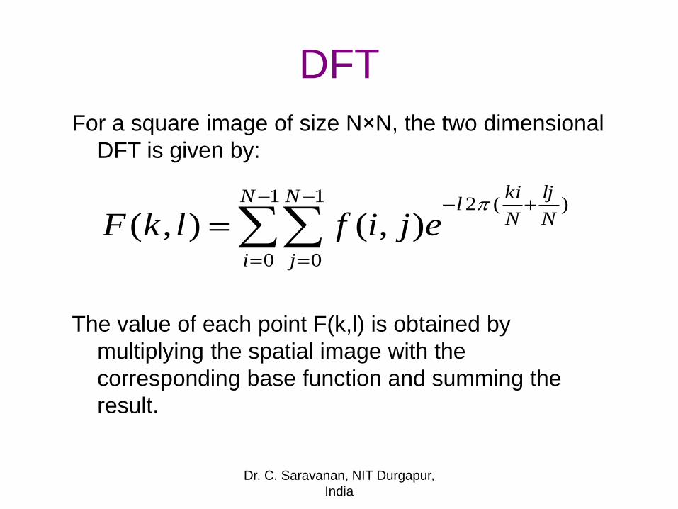
DFT

For a square image of size N×N, the two dimensional

DFT is given by:

1

0

1

0

)(2

),(),(N

i

N

j

N

lj

N

kil

ejiflkF

The value of each point F(k,l) is obtained by

multiplying the spatial image with the

corresponding base function and summing the

result.


India

Inverse DFT

1

0

1

0

)(2

2),(

1),(

N

k

N

l

N

lb

N

kal

elkFN

baF

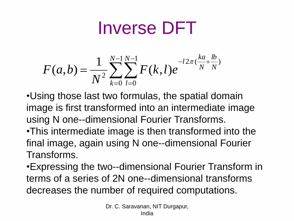
•Using those last two formulas, the spatial domain

image is first transformed into an intermediate image

using N one--dimensional Fourier Transforms.

•This intermediate image is then transformed into the

final image, again using N one--dimensional Fourier

Transforms.

•Expressing the two--dimensional Fourier Transform in

terms of a series of 2N one--dimensional transforms

decreases the number of required computations.


India

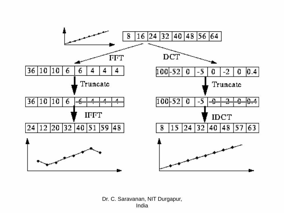
Discrete Cosine Transform (DCT)

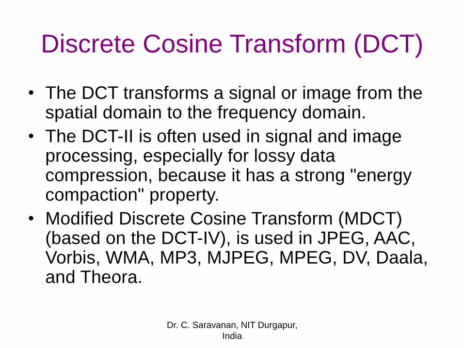
• The DCT transforms a signal or image from the spatial domain to the frequency domain.

• The DCT-II is often used in signal and image processing, especially for lossy data compression, because it has a strong "energy compaction" property.

• Modified Discrete Cosine Transform (MDCT) (based on the DCT-IV), is used in JPEG, AAC, Vorbis, WMA, MP3, MJPEG, MPEG, DV, Daala, and Theora.


India

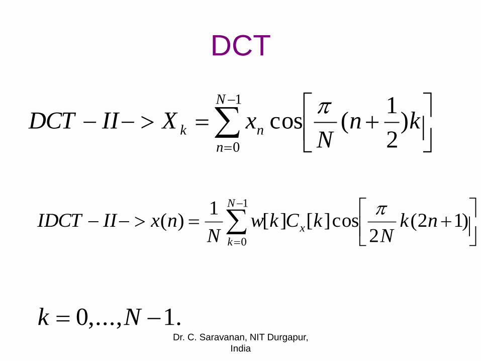
DCT

1

0

)2

1(cos

N

n

nk knN

xXIIDCT

.1,...,0 Nk

1

0

)12(2

cos][][1

)(N

k

x nkN

kCkwN

nxIIIDCT


India

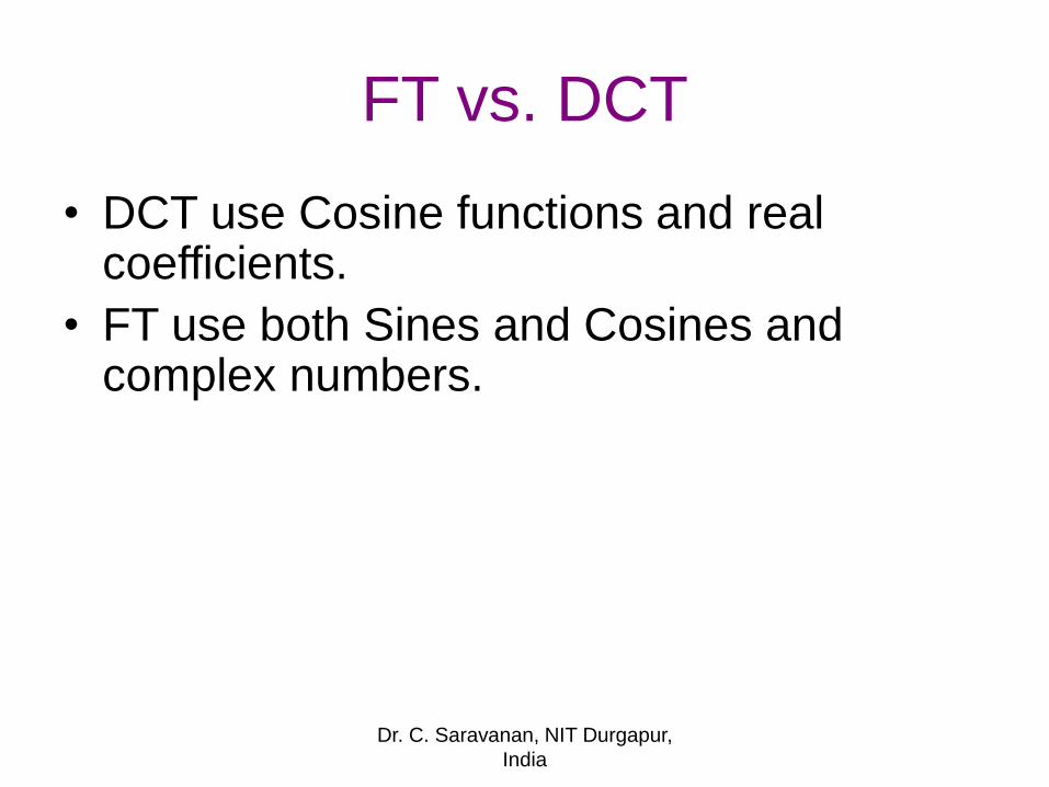
FT vs. DCT

• DCT use Cosine functions and real coefficients.

• FT use both Sines and Cosines and complex numbers.


India


India

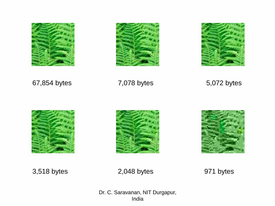
67,854 bytes 7,078 bytes 5,072 bytes

3,518 bytes 2,048 bytes 971 bytes


India

Discrete Wavelet Transform

• In mathematics, a wavelet series is a

representation of a square-integrable (real- or

complex-valued) function by a certain

orthonormal series generated by a wavelet.

• Wavelet-transformation contains information

similar to the short-time-Fourier-transformation,

but with additional properties of the wavelets,

which show up at the resolution in time at higher

analysis frequencies of the basis function.


India

DWT

• The discrete wavelet transform (DWT) is a linear transformation that operates on a data vector whose length is an integer power of two,transforming it into a numerically different vector of the same length.

• It is a tool that separates data into different frequency components, and then studies each component with resolution matched to its scale.


India

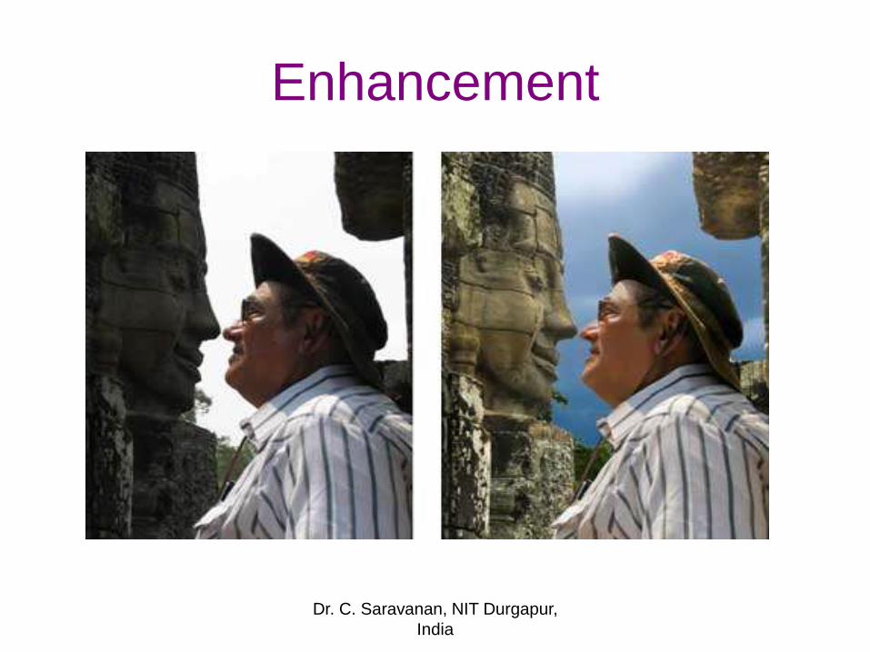
Enhancement


India

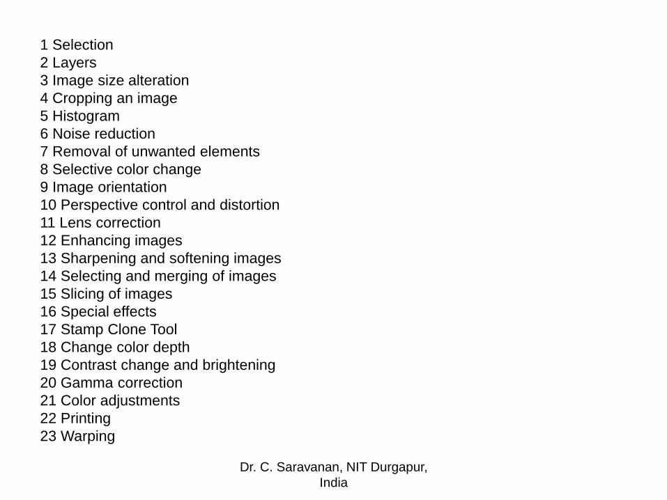
1 Selection

2 Layers

3 Image size alteration

4 Cropping an image

5 Histogram

6 Noise reduction

7 Removal of unwanted elements

8 Selective color change

9 Image orientation

10 Perspective control and distortion

11 Lens correction

12 Enhancing images

13 Sharpening and softening images

14 Selecting and merging of images

15 Slicing of images

16 Special effects

17 Stamp Clone Tool

18 Change color depth

19 Contrast change and brightening

20 Gamma correction

21 Color adjustments

22 Printing

23 Warping


India

Noise reduction

• Salt and pepper noise

• Gaussian noise

• Shot noise

• Quantization noise (uniform noise)

• Film grain

• Anisotropic noise


India

Image Compression

• Lossy and lossless compression

• Data compression refers to the process of reducing the amount of data required to represent given quantity of information.

• Data redundancy is the central concept in image compression and can be mathematically defined.

• IMAGE = INFORMATION + REDUNDANT DATA


India

Compression Ratio

• CR=n1 / n2

• CR - Compression Ratio

• n1 -Source image

• n2 - Compressed image


India

Types of Redundancy

• Coding redundancy

• Interpixel redundancy

• Psychovisual redundancy

• Coding Redundancy : A code is a system of symbols (i.e. bytes, bits) that represents information.

• Interpixel correlations

• Certain information has relatively less importance for the quality of image perception. This information is said to be psychovisually redundant.


India

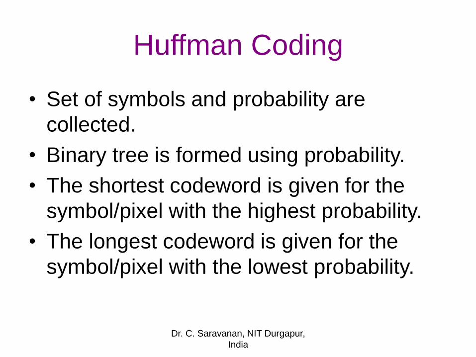
Huffman Coding

• Set of symbols and probability are

collected.

• Binary tree is formed using probability.

• The shortest codeword is given for the

symbol/pixel with the highest probability.

• The longest codeword is given for the

symbol/pixel with the lowest probability.


India

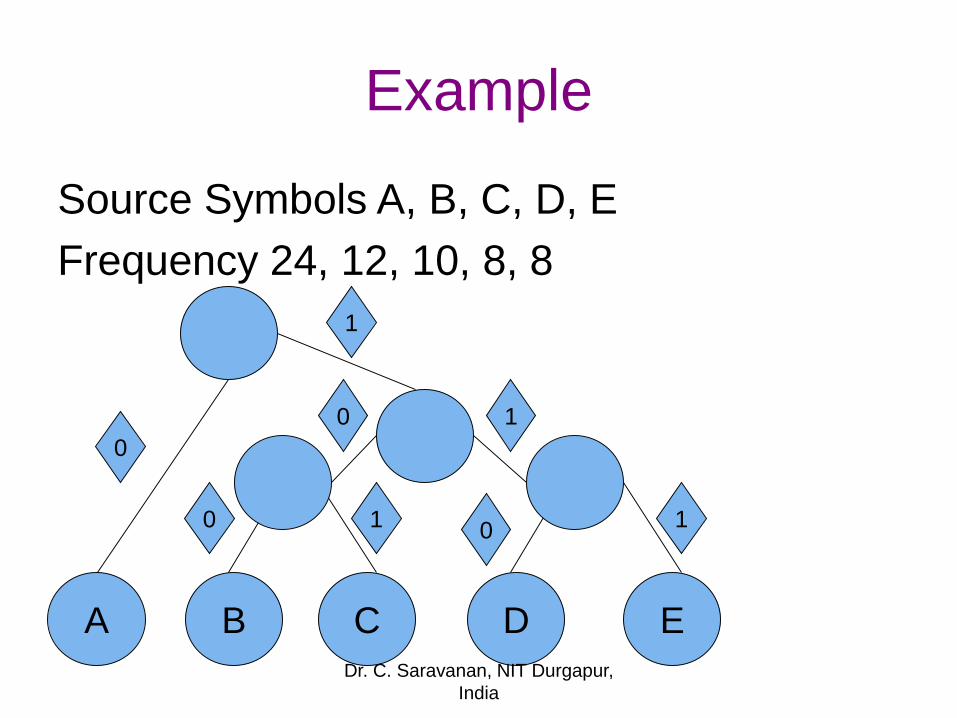
Example

Source Symbols A, B, C, D, E

Frequency 24, 12, 10, 8, 8

A B C D E

0

0 0

0

1

1 1

1


India

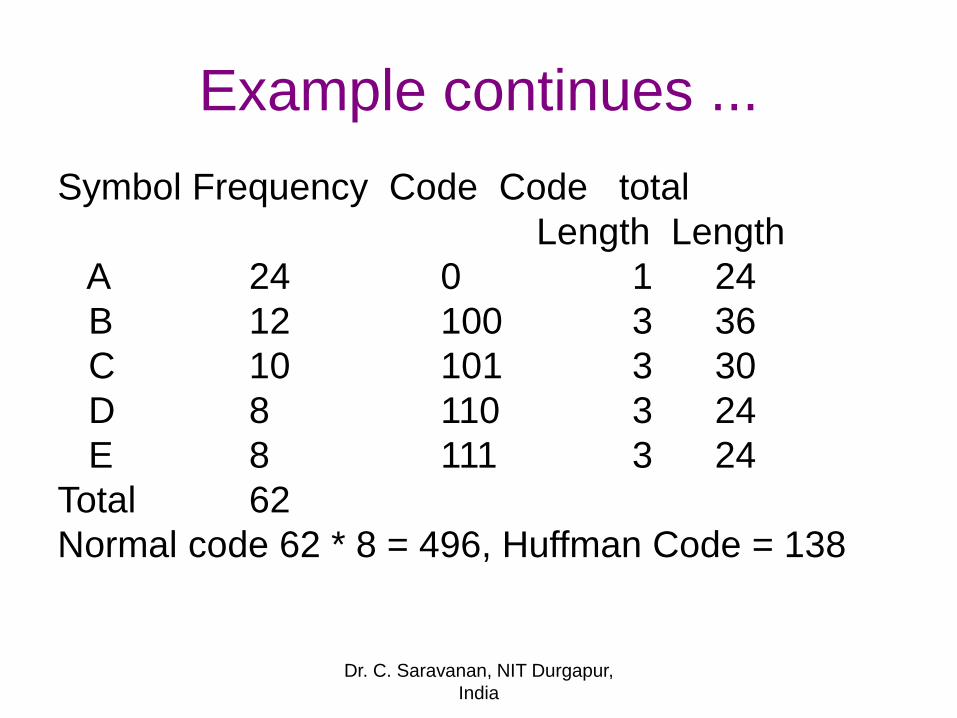
Example continues ...

Symbol Frequency Code Code total

Length Length

A 24 0 1 24

B 12 100 3 36

C 10 101 3 30

D 8 110 3 24

E 8 111 3 24

Total 62

Normal code 62 * 8 = 496, Huffman Code = 138


India

Arithmetic Coding

• A form of entropy encoding used in lossless data compression.

• Normally, a string of characters such as the words "hello there" is represented using a fixed number of bits per character, as in the ASCII code.

• Arithmetic coding encodes the entire message into a single number, a fraction nwhere (0.0 ≤ n < 1.0).


India

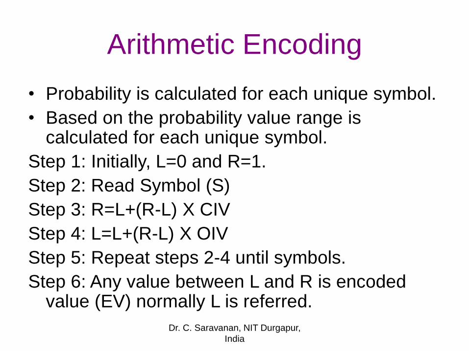
Arithmetic Encoding

• Probability is calculated for each unique symbol.

• Based on the probability value range is calculated for each unique symbol.

Step 1: Initially, L=0 and R=1.

Step 2: Read Symbol (S)

Step 3: R=L+(R-L) X CIV

Step 4: L=L+(R-L) X OIV

Step 5: Repeat steps 2-4 until symbols.

Step 6: Any value between L and R is encoded value (EV) normally L is referred.


India

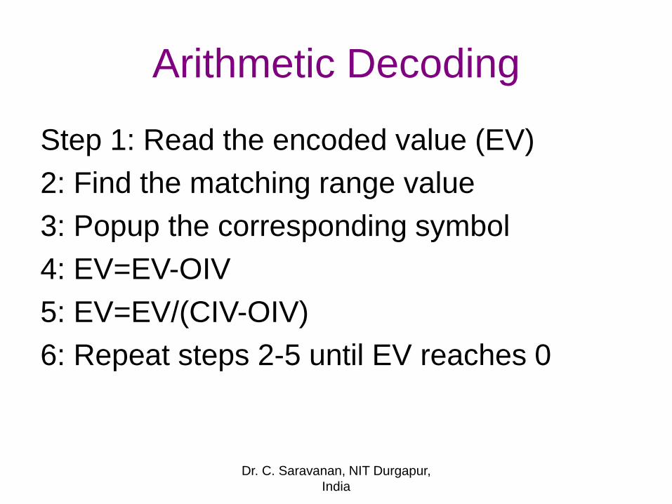
Arithmetic Decoding

Step 1: Read the encoded value (EV)

2: Find the matching range value

3: Popup the corresponding symbol

4: EV=EV-OIV

5: EV=EV/(CIV-OIV)

6: Repeat steps 2-5 until EV reaches 0


India

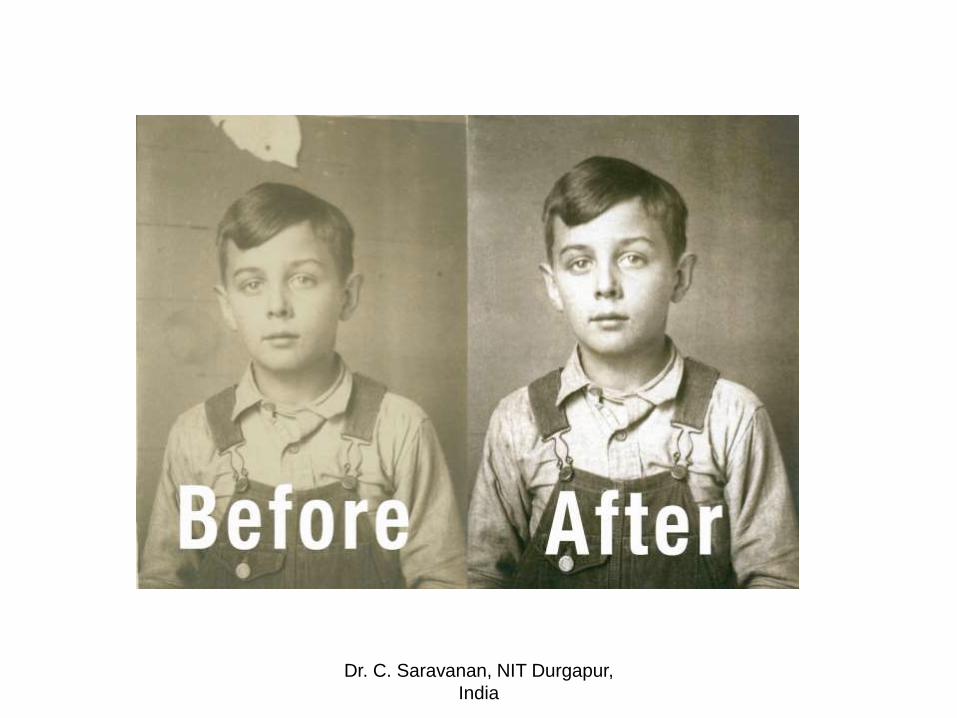
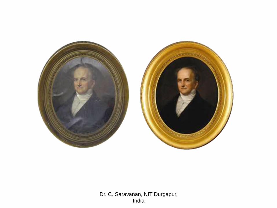
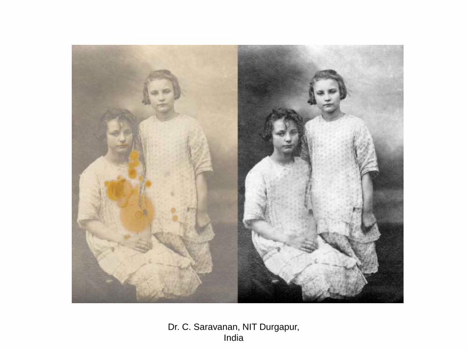
Image Restoration

• A photograph blurred by a defocused camera is analyzed to determine the nature of the blur.

• Degradation comes in many forms such as motion blur, noise, and camera misfocus.

• It is possible to come up with an very good estimate of the actual blurring function and "undo" the blur to restore the original image


India


India

Application Domains

• Scientific explorations

• Legal investigations

• Film making and archival

• Image and video (de-)coding

....

• Consumer photography


India

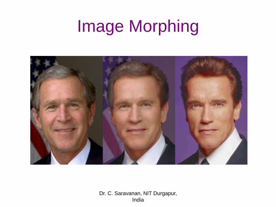
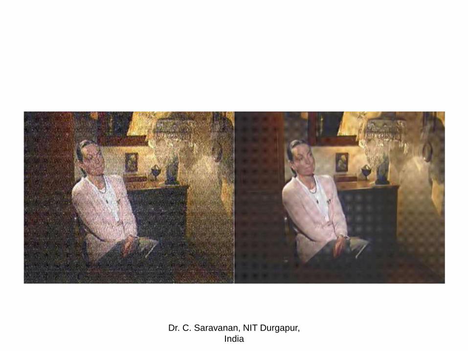
Image Morphing


India

• Depict one person turning into another

• Morphing is a special effect in motion

pictures and animations that changes (or

morphs) one image or shape into another

through a seamless transition.

• Achieved through cross-fading techniques


India

• Morphing is an image processing

technique used for the metamorphosis

from one image to another.

• Cross-dissolve between them

• The color of each pixel is interpolated over

time from the first image value to the

corresponding second image value.


India

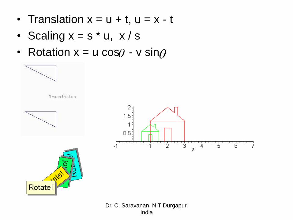
• Translation x = u + t, u = x - t

• Scaling x = s * u, x / s

• Rotation x = u cos - v sin


India

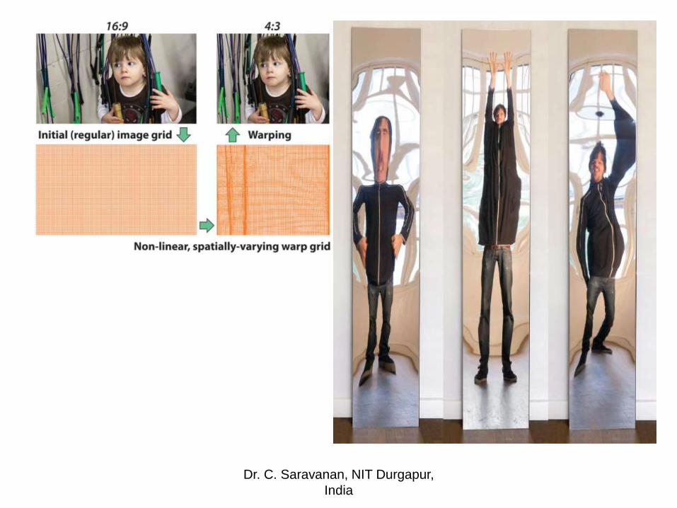
Image Warping

• Warping may be used for correcting image

distortion and for creative purposes.

• Points are mapped to points without

changing the colors.

• Applications - Cartoon Pictures and

Movies.


India


India

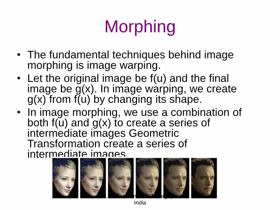
Morphing

• The fundamental techniques behind image morphing is image warping.

• Let the original image be f(u) and the final image be g(x). In image warping, we create g(x) from f(u) by changing its shape.

• In image morphing, we use a combination of both f(u) and g(x) to create a series of intermediate images Geometric Transformation create a series of intermediate images.


India

Image Restoration

• To remove or reduce the degradations.

• The degradations may be due to

– sensor noise

– blur due to camera misfocus

– relative object-camera motion

– random atmospheric turbulence

– others


India

Restoration Methods

• Deterministic– work with sample by sample processing

• Stochastic– work with the statistics of the image

• Non-blind– The degradation process is known

• Blind– The degradation process is unknown

• Direct, Iterative, and Recursive (implementation)


India

Restoration Domain

• Restoration techniques are best in the

spatial domain - scanned old images - not

occured at the time of image acquiring.

• Spatial processing is applicable if the

degradation is additive noise.

• Frequency domain filters too used.


India

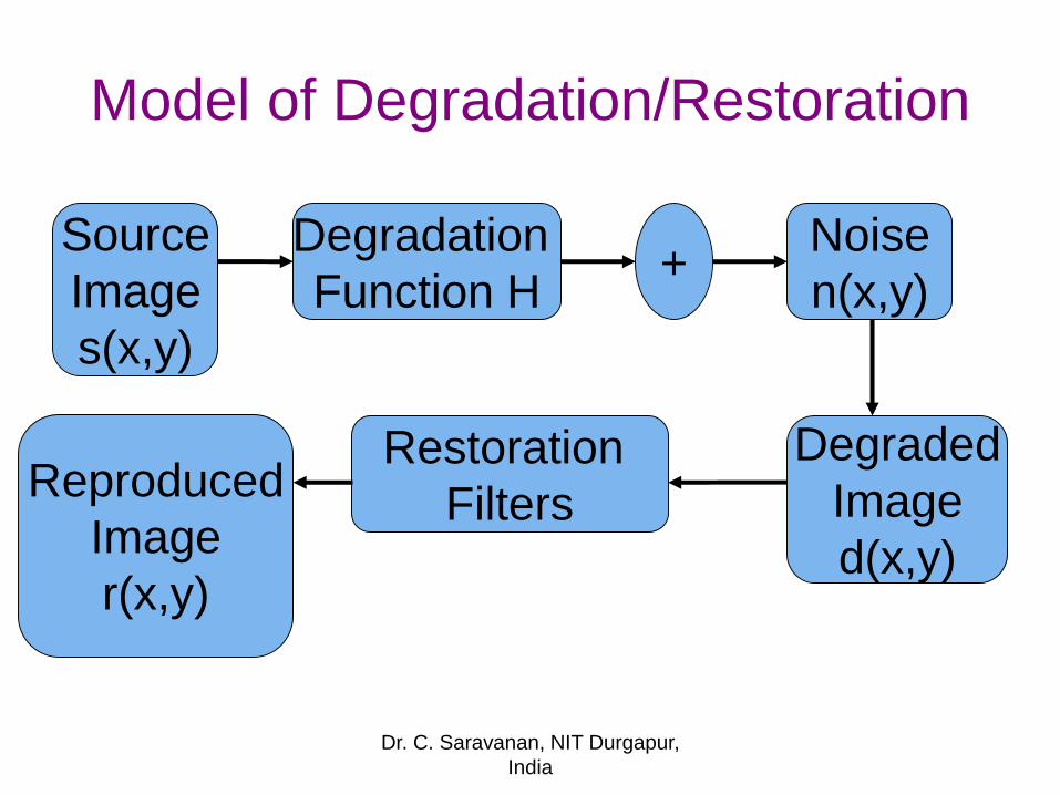
Model of Degradation/Restoration

Source

Image

s(x,y)

Degradation

Function H

Noise

n(x,y)+

Degraded

Image

d(x,y)

Restoration

FiltersReproduced

Image

r(x,y)


India

Estimation of Restoration

• Objective of restoration is to estimate

r(x,y) using

– Degraded image d(x,y)

– Knowledge of degraded function H

– Knowledge of additive noise n(x,y)

• The estimate should be as close as

possible to the source image s(x,y).


India

Enhancement Vs. Restoration

• Reconstruction techniques are oriented toward modeling the degradation.

• Applying the inverse process for recovering the original image.

• Restoration - Deblurring - removal of blur.

• Enhancement - Contrast Stretching -improves the visual quality of the image.

• Enhancement is Subjective and Restoration is Objective.


India

Noise

• Digital image has several different noise sources, some of them fixed, some temporal, some are temperature dependent.

• The noise characteristics of the camera are analyzed by shooting numerous frames both in complete darkness (for dark signal and noise properties) with several exposure times and on different exposure levels with flat field target.


India

Noise

• Principal source of noise - image acquisition (digitisation) - transmission.

• Performance of imaging sensors are affected by environmental conditions and quality of sensing elements.

• Light levels and sensor temperature -major factors.

• Transmission - Wireless - Atmospheric disturbance - Lightning.


India

• Based on these measurements, several parameters describing camera’s noise characteristics and sensitivity are calculated.

• These parameters include for example camera gain constant (electrons/output digital number), dark signal nonuniformity, photoresponse nonuniformity and STDs of temporal noise and fixed pattern noise.

Characterisation of Noise


India

Types of Noise

• Noise components divided into three groups: signal dependent, temperature dependent and time dependent.

• Signal dependent noise components are photon shot noise, photoresponse nonuniformity (PRNU) and amplifier gain non-uniformity.


India

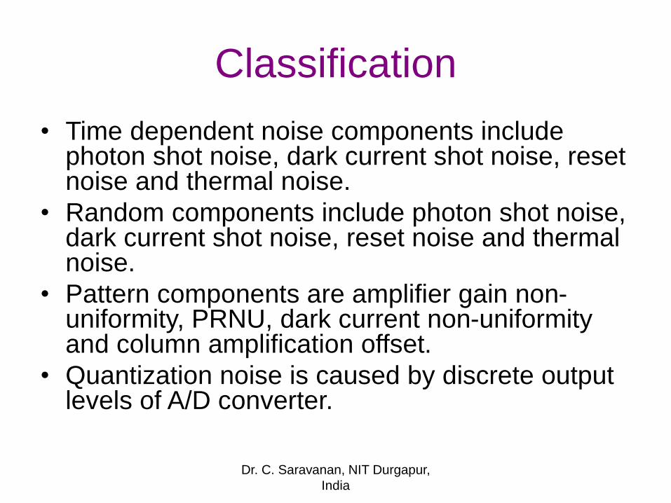
Classification

• Time dependent noise components include photon shot noise, dark current shot noise, reset noise and thermal noise.

• Random components include photon shot noise, dark current shot noise, reset noise and thermal noise.

• Pattern components are amplifier gain non-uniformity, PRNU, dark current non-uniformity and column amplification offset.

• Quantization noise is caused by discrete output levels of A/D converter.


India

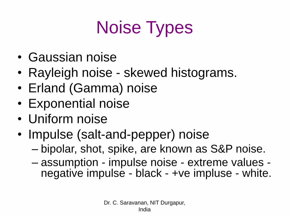
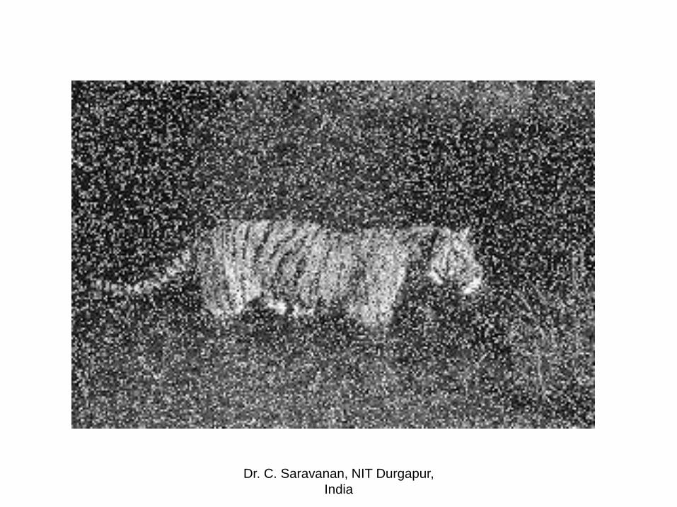
Noise Types

• Gaussian noise

• Rayleigh noise - skewed histograms.

• Erland (Gamma) noise

• Exponential noise

• Uniform noise

• Impulse (salt-and-pepper) noise– bipolar, shot, spike, are known as S&P noise.

– assumption - impulse noise - extreme values -negative impulse - black - +ve impluse - white.


India

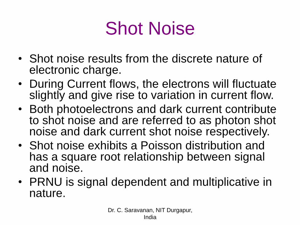
Shot Noise

• Shot noise results from the discrete nature of electronic charge.

• During Current flows, the electrons will fluctuate slightly and give rise to variation in current flow.

• Both photoelectrons and dark current contribute to shot noise and are referred to as photon shot noise and dark current shot noise respectively.

• Shot noise exhibits a Poisson distribution and has a square root relationship between signal and noise.

• PRNU is signal dependent and multiplicative in nature.


India

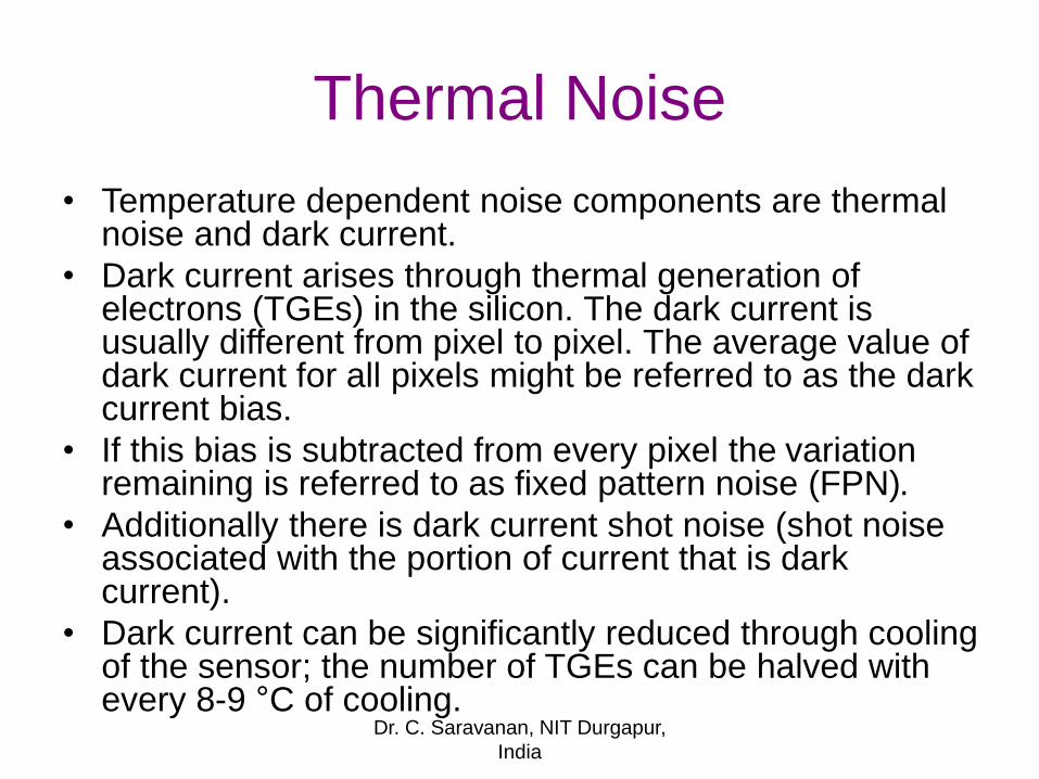
Thermal Noise

• Temperature dependent noise components are thermal noise and dark current.

• Dark current arises through thermal generation of electrons (TGEs) in the silicon. The dark current is usually different from pixel to pixel. The average value of dark current for all pixels might be referred to as the dark current bias.

• If this bias is subtracted from every pixel the variation remaining is referred to as fixed pattern noise (FPN).

• Additionally there is dark current shot noise (shot noise associated with the portion of current that is dark current).

• Dark current can be significantly reduced through cooling of the sensor; the number of TGEs can be halved with every 8-9 °C of cooling.


India

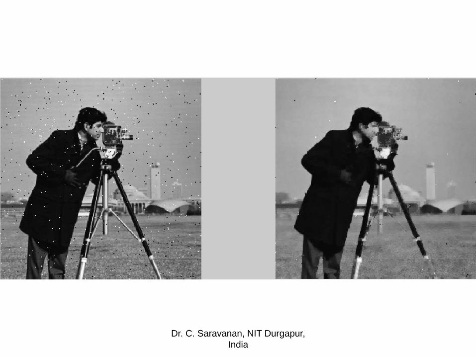
Salt and Pepper Noise

• Also known as Impulse Noise.

• Cause by sharp & sudden disturbance in

the image signal.

• Sparsely occurring white and black pixels.

• Certain amount of the pixels in the image

are either black or white.

• Median Filter

• Morphological Filter


India

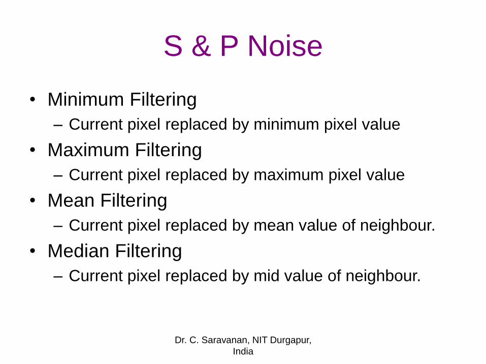
S & P Noise

• Minimum Filtering

– Current pixel replaced by minimum pixel value

• Maximum Filtering

– Current pixel replaced by maximum pixel value

• Mean Filtering

– Current pixel replaced by mean value of neighbour.

• Median Filtering

– Current pixel replaced by mid value of neighbour.


India

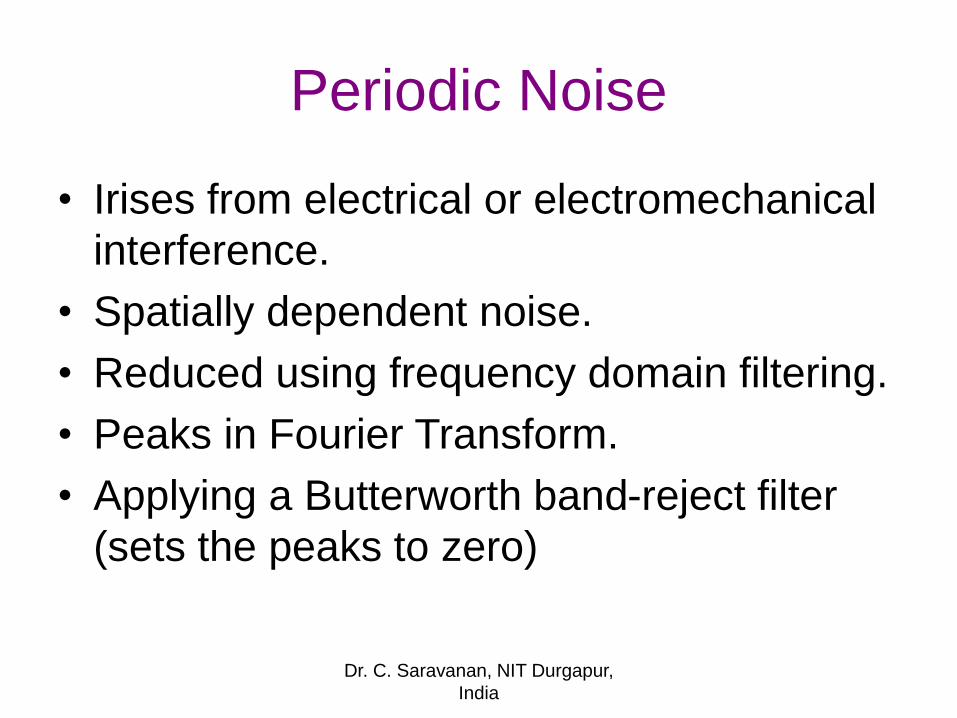
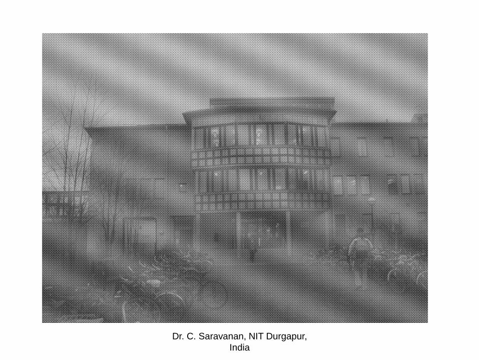
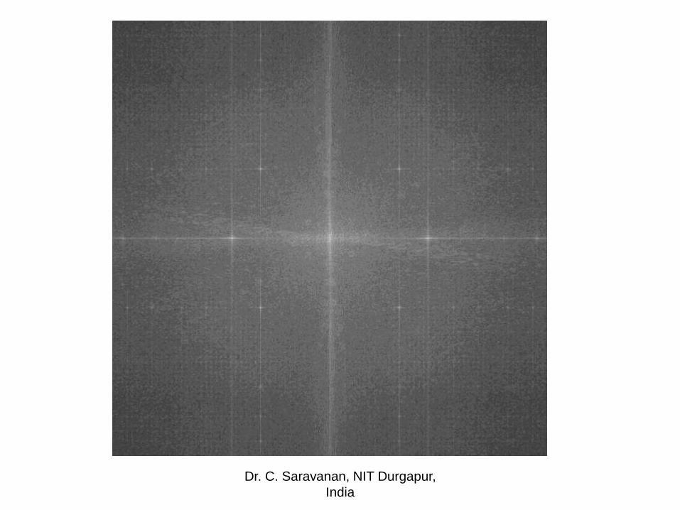
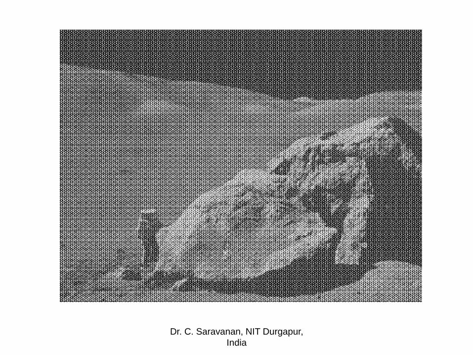
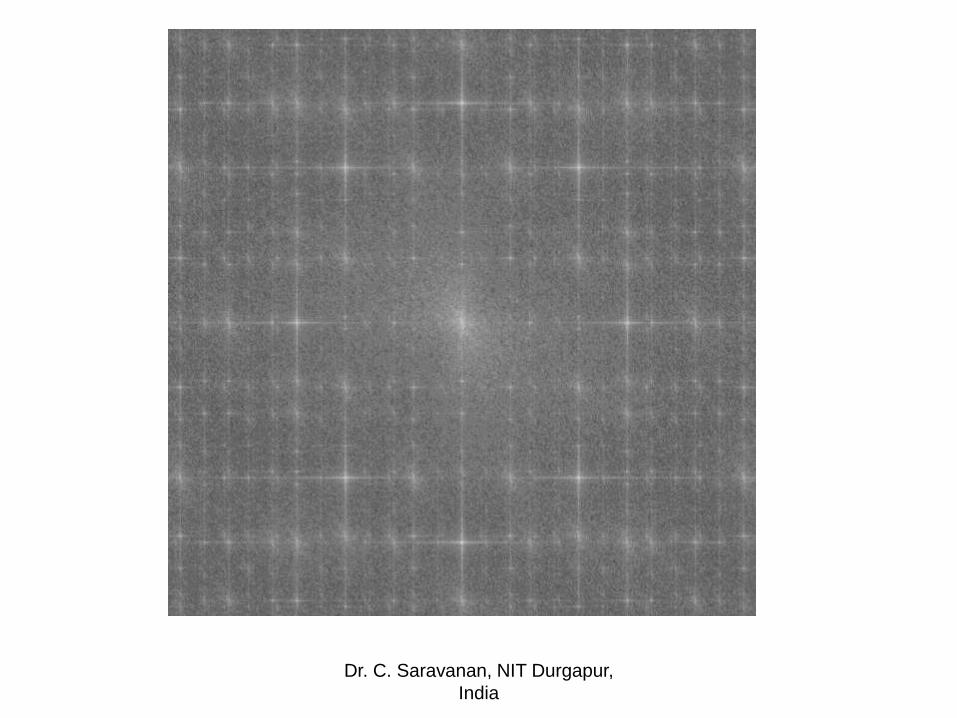
Periodic Noise

• Irises from electrical or electromechanical

interference.

• Spatially dependent noise.

• Reduced using frequency domain filtering.

• Peaks in Fourier Transform.

• Applying a Butterworth band-reject filter

(sets the peaks to zero)


India


India

Gaussian Noise

• Karl Friedrich Gauss, an 18th century German physicist

• Is caused by Random fluctuations

• Also called statistical noise

• Gaussian noise in digital images arise during acquisition.

• Sensor noise caused by poor illumination and/or high temperature, and/or transmission e.g. electronic circuit noise


India


India

Estimating Noise Parameters

• Choose an Optical sensor

• Preoare a solid gray board

• Set up an uniform illumination

• Capture set of images

• Resulting images are indicators of system

noise.


India

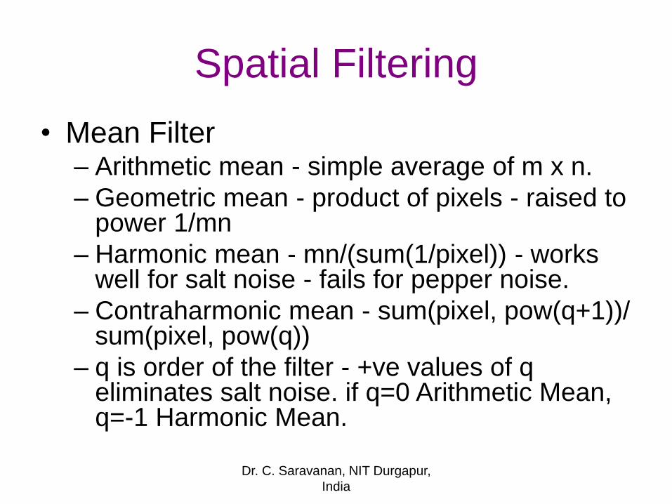
Spatial Filtering

• Mean Filter– Arithmetic mean - simple average of m x n.

– Geometric mean - product of pixels - raised to power 1/mn

– Harmonic mean - mn/(sum(1/pixel)) - works well for salt noise - fails for pepper noise.

– Contraharmonic mean - sum(pixel, pow(q+1))/ sum(pixel, pow(q))

– q is order of the filter - +ve values of q eliminates salt noise. if q=0 Arithmetic Mean, q=-1 Harmonic Mean.


India

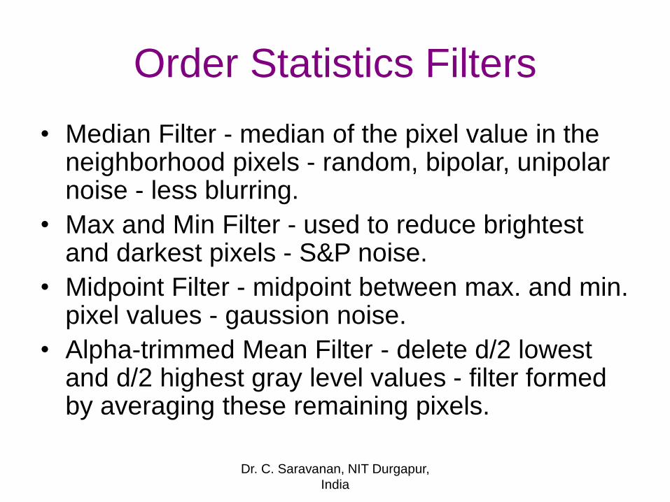
Order Statistics Filters

• Median Filter - median of the pixel value in the neighborhood pixels - random, bipolar, unipolar noise - less blurring.

• Max and Min Filter - used to reduce brightest and darkest pixels - S&P noise.

• Midpoint Filter - midpoint between max. and min. pixel values - gaussion noise.

• Alpha-trimmed Mean Filter - delete d/2 lowest and d/2 highest gray level values - filter formed by averaging these remaining pixels.


India

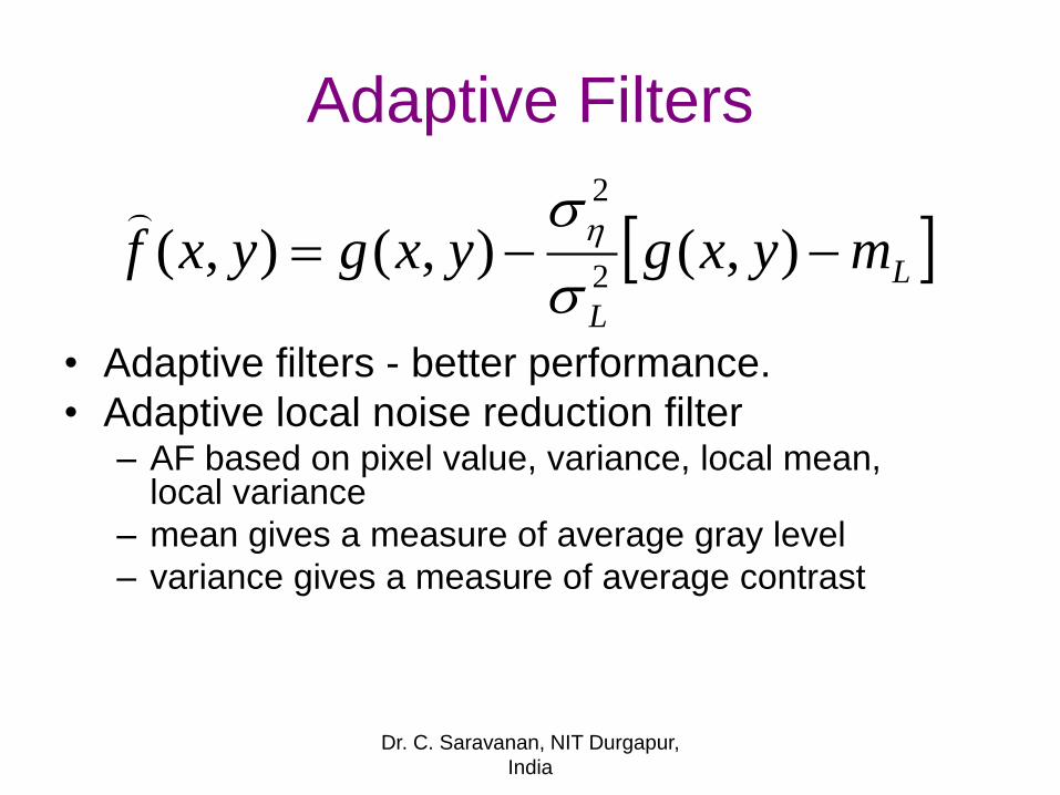
Adaptive Filters

• Adaptive filters - better performance.

• Adaptive local noise reduction filter– AF based on pixel value, variance, local mean,

local variance

– mean gives a measure of average gray level

– variance gives a measure of average contrast

L

L

myxgyxgyxf ),(),(),(2

2


India

Adaptive Median Filter

• AMF can handle impulse noise with larger probabilities compared to median filter -preserves details while smoothing.

• sxy is rectangular working area

• zmin = minimum gray level in sxy

• zmax = maximum gray level in sxy

• zmed = median of gray level in sxy

• zxy = gray level at coordinates (x,y)

• smax = maximum allowed size of sxy.


India

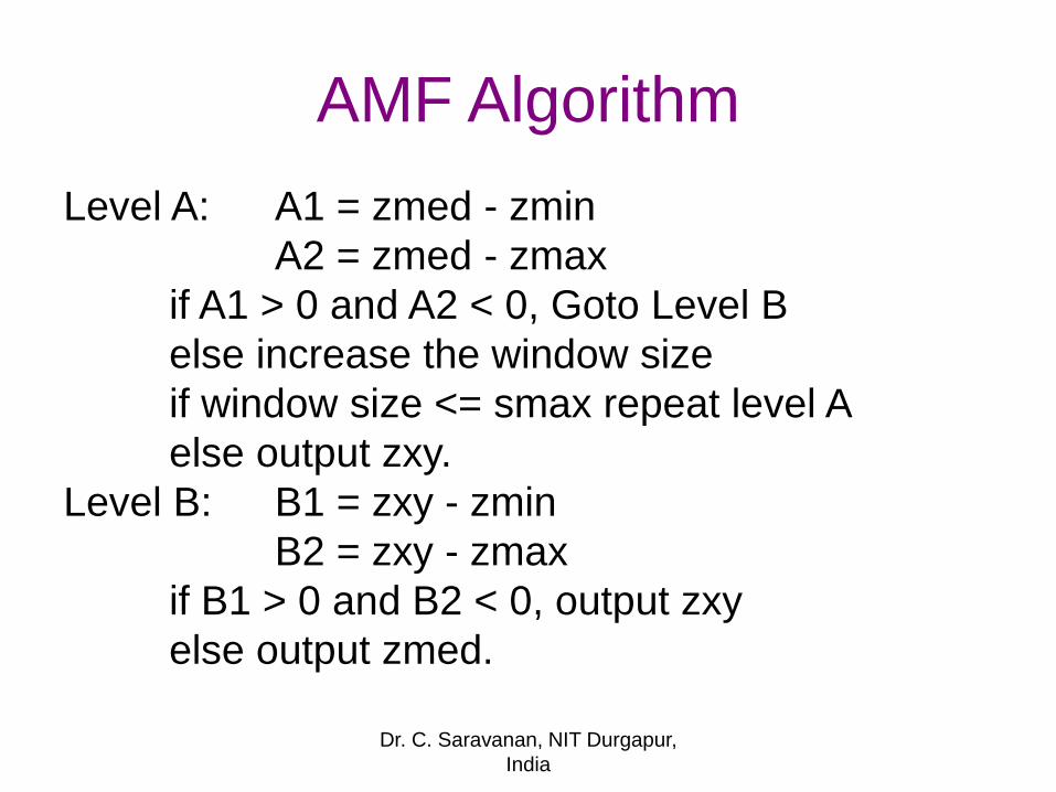
AMF Algorithm

Level A: A1 = zmed - zmin

A2 = zmed - zmax

if A1 > 0 and A2 < 0, Goto Level B

else increase the window size

if window size <= smax repeat level A

else output zxy.

Level B: B1 = zxy - zmin

B2 = zxy - zmax

if B1 > 0 and B2 < 0, output zxy

else output zmed.


India

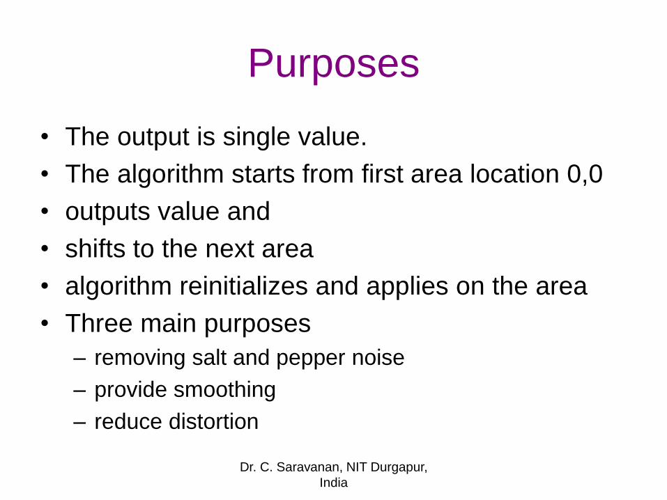
Purposes

• The output is single value.

• The algorithm starts from first area location 0,0

• outputs value and

• shifts to the next area

• algorithm reinitializes and applies on the area

• Three main purposes

– removing salt and pepper noise

– provide smoothing

– reduce distortion


India

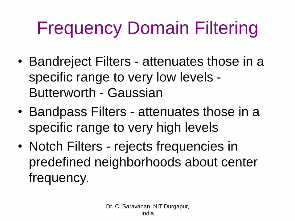
Frequency Domain Filtering

• Bandreject Filters - attenuates those in a

specific range to very low levels -

Butterworth - Gaussian

• Bandpass Filters - attenuates those in a

specific range to very high levels

• Notch Filters - rejects frequencies in

predefined neighborhoods about center

frequency.


India

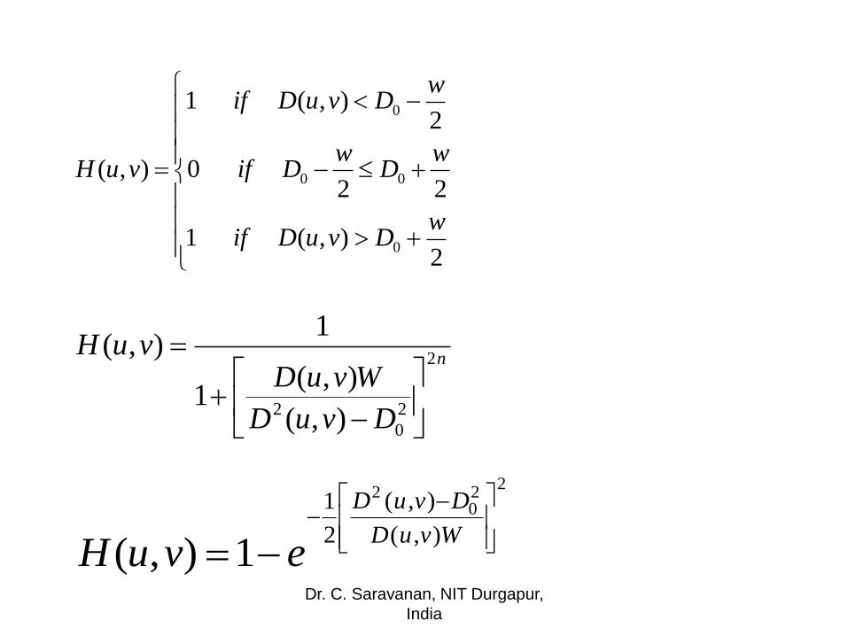
2),(1

220

2),(1

),(

0

00

0

wDvuDif

wD

wDif

wDvuDif

vuH

n

DvuD

WvuDvuH

2

2

0

2 ),(

),(1

1),(

220

2

),(

),(

2

1

1),(

WvuD

DvuD

evuHDr. C. Saravanan, NIT Durgapur,

India

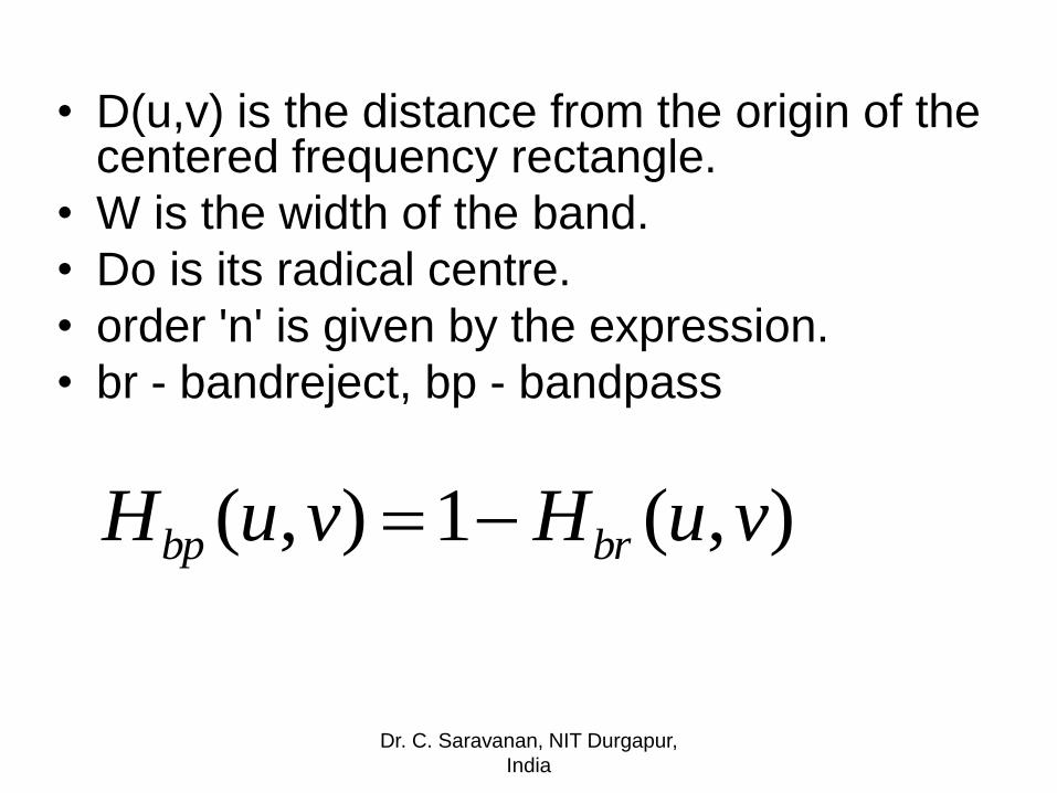
• D(u,v) is the distance from the origin of the centered frequency rectangle.

• W is the width of the band.

• Do is its radical centre.

• order 'n' is given by the expression.

• br - bandreject, bp - bandpass

),(1),( vuHvuH brbp


India

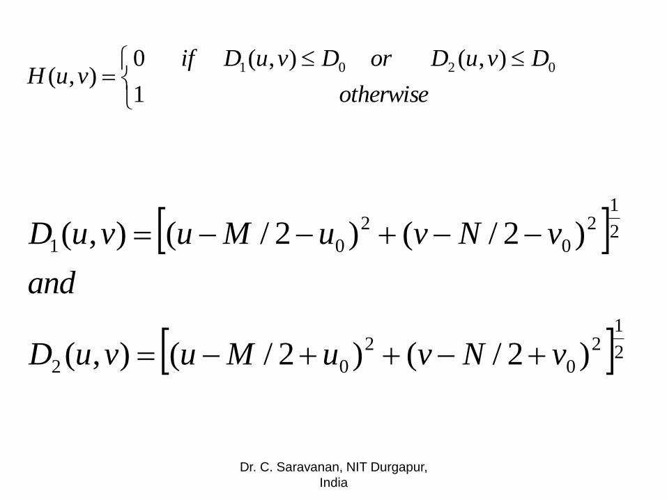
otherwise

DvuDorDvuDifvuH

0201 ),(),(

1

0),(

21

2

0

2

02

2

12

0

2

01

)2/()2/(),(

)2/()2/(),(

vNvuMuvuD

and

vNvuMuvuD


India

Estimating the Degrading Function

• Observation - degraded image - no knowledge - gather information from the image itself - uniform background regions -strong signal content - estimate the power spectrum or the probability density function - studying the mechanism that caused the degradation.

• Experimentation - equivalent equipment

• Mathematical Modeling


India

Inverse Filtering

• If we know of or can create a good model of the blurring function that corrupted an image, the quickest and easiest way to restore that is by inverse filtering.

• The inverse filter is a form of high pass filter.

• Noise tends to be high frequency.

• Thresholding and an Iterative method.


India

Weiner Filtering

• also called Minimum Mean Square Error

Filter or Least Square Error Filter

• its a statistical approach.

• incorporates both the degradation function

and statistical characteristics of noise.

• noise and image are uncorrelated.


India

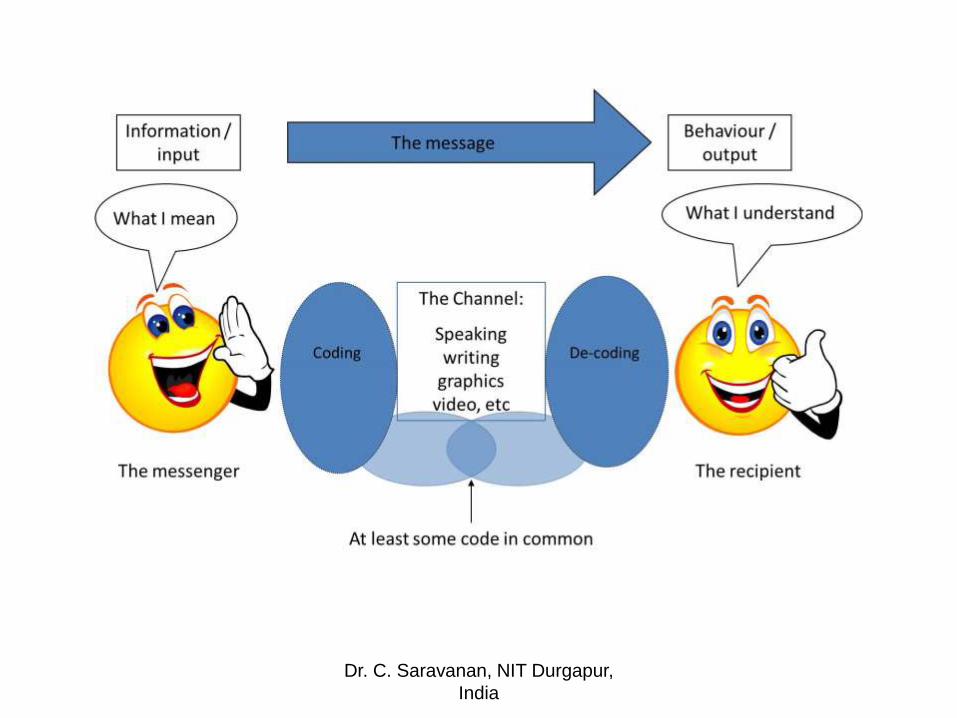
Encoder and Decoder Model

• The Encoding/decoding model of

communication was first developed by

cultural studies scholar Stuart Hall in 1973,

titled 'Encoding and Decoding in the

Television Discourse,'

• Hall's essay offers a theoretical approach

of how media messages are produced,

disseminated, and interpreted.


India

http://en.wikipedia.org/wiki/Stuart_Hall_(cultural_theorist)


India

Three different positions

• For example, advertisements can have

multiple layers of meaning, they can be

decoded in various ways and can mean

something different to different people.

• Decoding subject can assume three

different positions: Dominant/hegemonic

position, negotiated position, and

oppositional position.


India

Four-stage model

• Production – This is where the encoding of a

message takes place.

• Circulation – How individuals perceive things:

visual vs. written.

• Use (distribution or consumption) – This is the

decoding/interpreting of a message which

requires active recipients.

• Reproduction – This is the stage after audience

members have interpreted the message in their

own way based on their experiences and beliefs.Dr. C. Saravanan, NIT Durgapur,

India

Dominant/hegemonic position

• This position is one where the consumer takes

the actual meaning directly, and decodes it

exactly the way it was encoded.

• The consumer is located within the dominant

point of view, and is fully sharing the texts codes

and accepts and reproduces the intended

meaning.

• Here, there is barely any misunderstanding

because both the sender and receiver have the

same cultural biases.


India

Negotiated position

• This position is a mixture of accepting and

rejecting elements.

• Readers are acknowledging the dominant

message, but are not willing to completely

accept it the way the encoder has

intended.

• The reader to a certain extent shares the

texts code and generally accepts the

preferred meaningDr. C. Saravanan, NIT Durgapur,

India

Oppositional position

• In this position a consumer understands

the literal meaning, but due to different

backgrounds each individual has their own

way of decoding messages, while forming

their own interpretations.

• The readers' social situation has placed

them in a directly oppositional relation to

the dominant code.


India

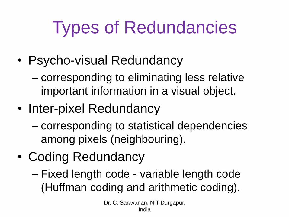
Types of Redundancies

• Psycho-visual Redundancy

– corresponding to eliminating less relative

important information in a visual object.

• Inter-pixel Redundancy

– corresponding to statistical dependencies

among pixels (neighbouring).

• Coding Redundancy

– Fixed length code - variable length code

(Huffman coding and arithmetic coding).


India

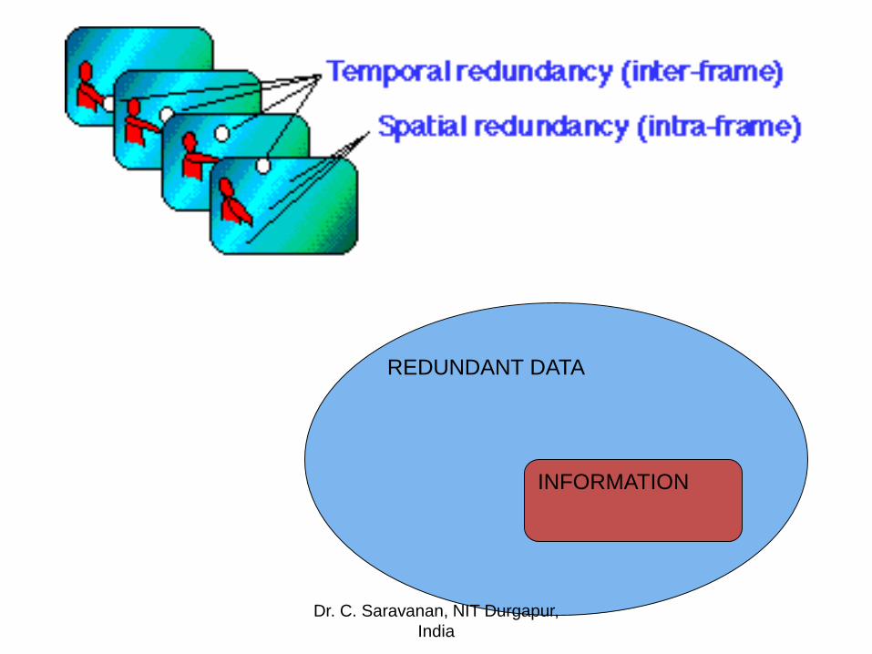
REDUNDANT DATA

INFORMATION


India

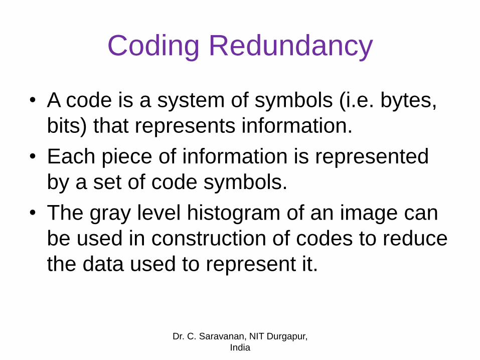
Coding Redundancy

• A code is a system of symbols (i.e. bytes,

bits) that represents information.

• Each piece of information is represented

by a set of code symbols.

• The gray level histogram of an image can

be used in construction of codes to reduce

the data used to represent it.


India

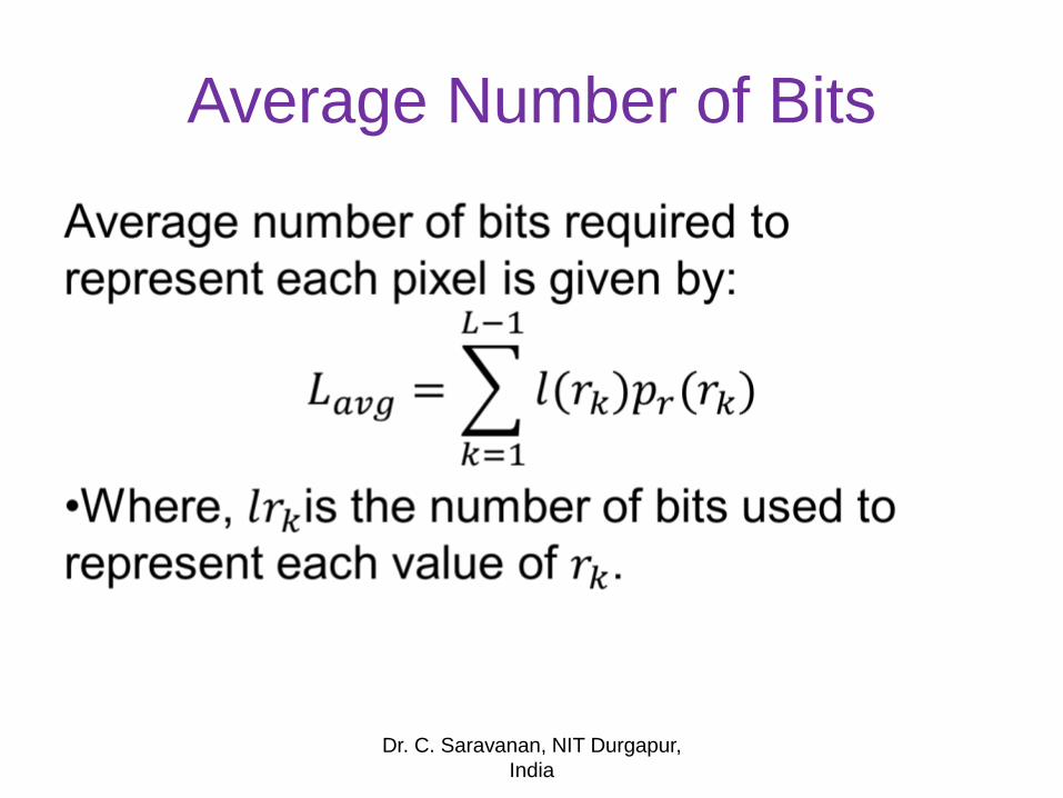
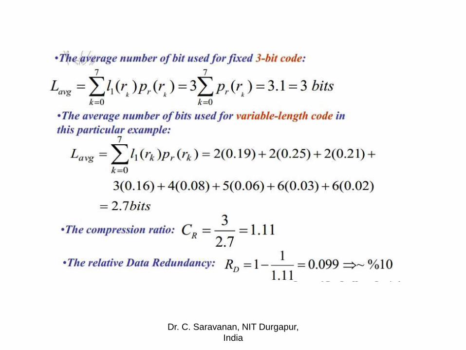
Average Number of Bits


India


India

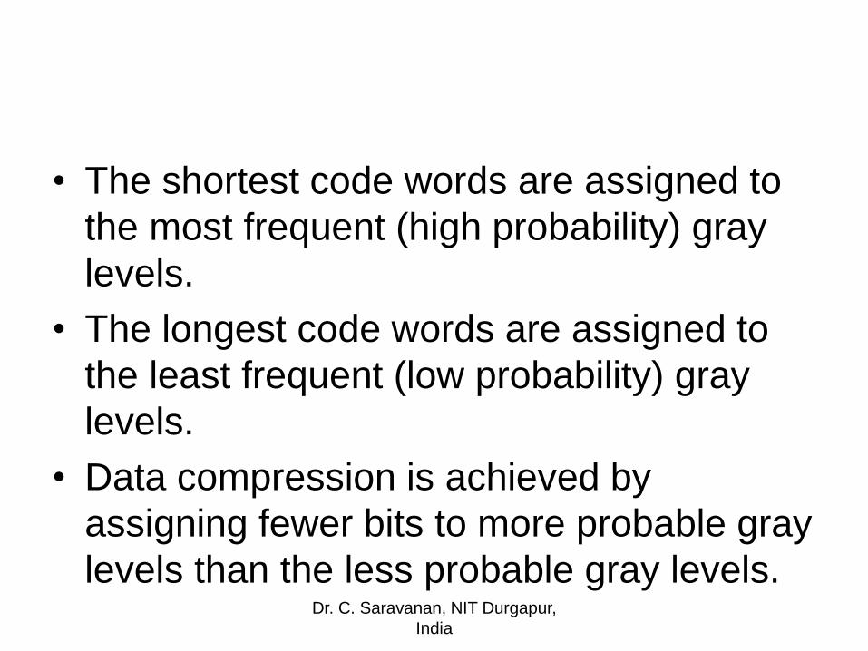
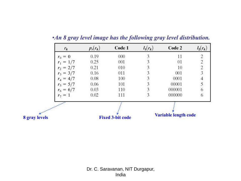
• The shortest code words are assigned to

the most frequent (high probability) gray

levels.

• The longest code words are assigned to

the least frequent (low probability) gray

levels.

• Data compression is achieved by

assigning fewer bits to more probable gray

levels than the less probable gray levels.Dr. C. Saravanan, NIT Durgapur,

India

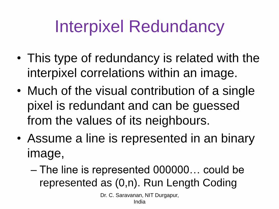
Interpixel Redundancy

• This type of redundancy is related with the

interpixel correlations within an image.

• Much of the visual contribution of a single

pixel is redundant and can be guessed

from the values of its neighbours.

• Assume a line is represented in an binary

image,

– The line is represented 000000… could be

represented as (0,n). Run Length CodingDr. C. Saravanan, NIT Durgapur,

India

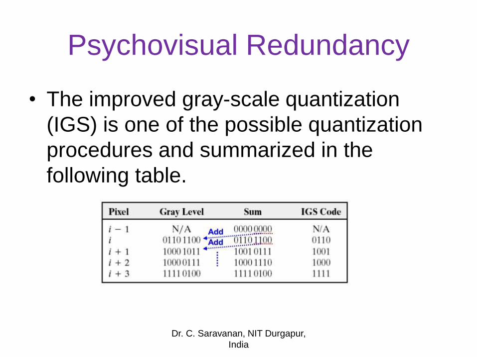
Psychovisual Redundancy

• The improved gray-scale quantization

(IGS) is one of the possible quantization

procedures and summarized in the

following table.


India

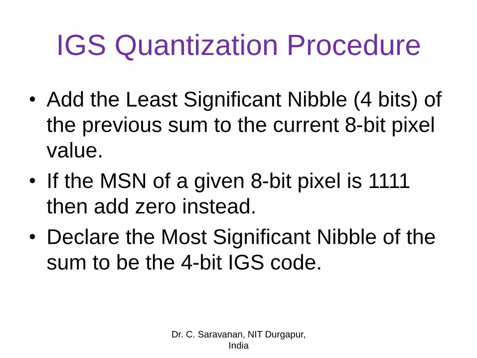
IGS Quantization Procedure

• Add the Least Significant Nibble (4 bits) of

the previous sum to the current 8-bit pixel

value.

• If the MSN of a given 8-bit pixel is 1111

then add zero instead.

• Declare the Most Significant Nibble of the

sum to be the 4-bit IGS code.


India

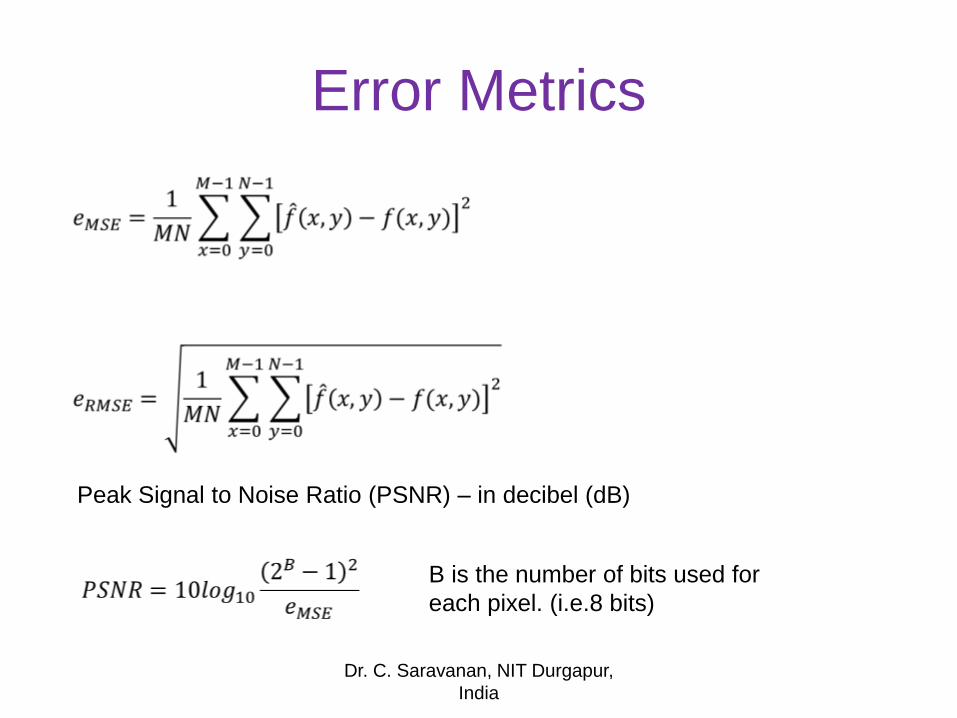
Error Metrics

B is the number of bits used for

each pixel. (i.e.8 bits)

Peak Signal to Noise Ratio (PSNR) – in decibel (dB)


India

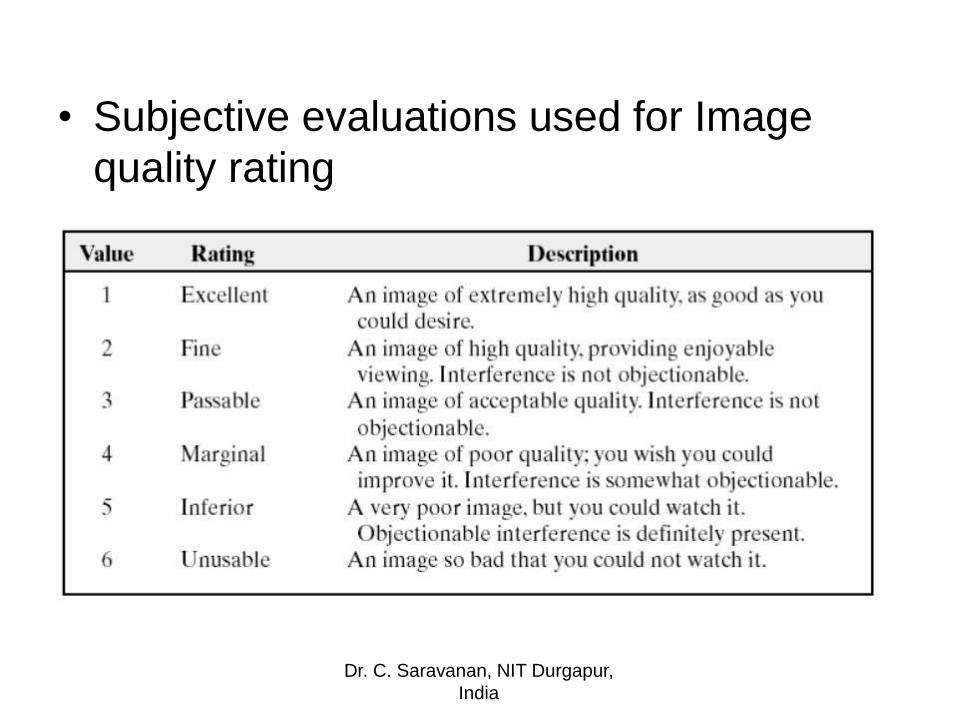
• Subjective evaluations used for Image

quality rating


India

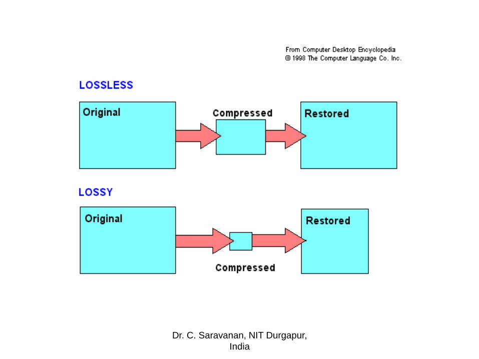
Lossy Compression

• "Lossy" compression is the class of data encoding methods that uses inexact approximations (or partial data discarding) for representing the content that has been encoded.

• Lossy compression technologies attempt to eliminate redundant or unnecessary information.

• Most video and audio compression technologies use a lossy technique.

• Compromise in the accuracy of the reconstructed image - distortion to a level of acceptance


India


India

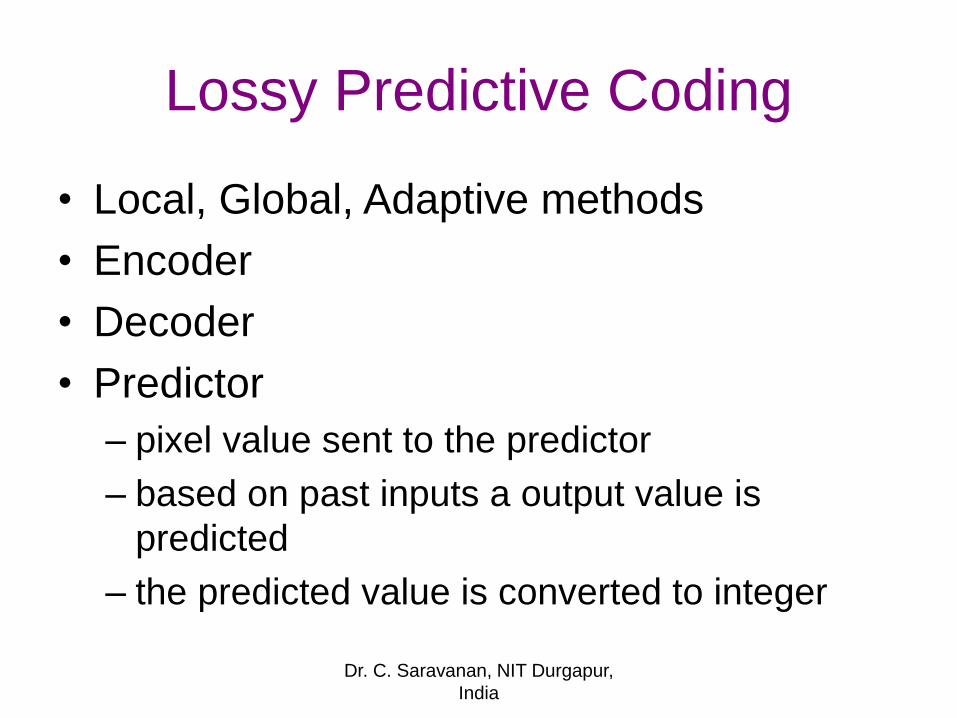
Lossy Predictive Coding

• Local, Global, Adaptive methods

• Encoder

• Decoder

• Predictor

– pixel value sent to the predictor

– based on past inputs a output value is

predicted

– the predicted value is converted to integer


India

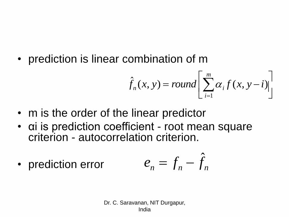
nnn ffe ˆ

m

i

in iyxfroundyxf1

),(),(ˆ

• prediction is linear combination of m

• m is the order of the linear predictor

• αi is prediction coefficient - root mean square criterion - autocorrelation criterion.

• prediction error


India

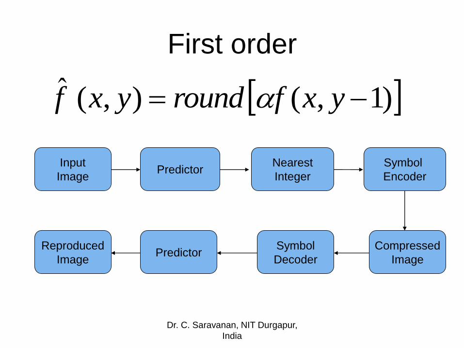
First order

)1,(),(ˆ yxfroundyxf

Input

ImagePredictor

Nearest

Integer

Symbol

Encoder

Compressed

Image

Symbol

DecoderPredictor

Reproduced

Image


India

Transform Coding

• Reversible, Linear transform such as Fourier Transform is used.

• Transform coding is used to convert spatial image pixel values to transform coefficient values.

• Since this is a linear process and no information is lost, the number of coefficients produced is equal to the number of pixels transformed.


India

• The desired effect is that most of the

energy in the image will be contained in a

few large transform coefficients.

• If it is generally the same few coefficients

that contain most of the energy in most

pictures, then the coefficients may be

further coded by lossless entropy coding.


India

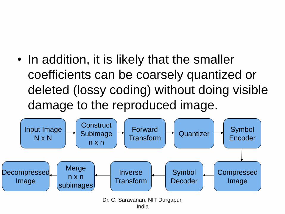
• In addition, it is likely that the smaller

coefficients can be coarsely quantized or

deleted (lossy coding) without doing visible

damage to the reproduced image.

Input Image

N x N

Forward

TransformQuantizer

Symbol

Encoder

Construct

Subimage

n x n

Compressed

Image

Inverse

Transform

Symbol

Decoder

Merge

n x n

subimages

Decompressed

Image


India

• Fourier Transform

• Karhonen-Loeve Transform (KLT)

• Walsh-Hadamard Transform

• Lapped orthogonal Transform

• Discrete Cosine Transform (DCT)

• Wavelets Transform


India

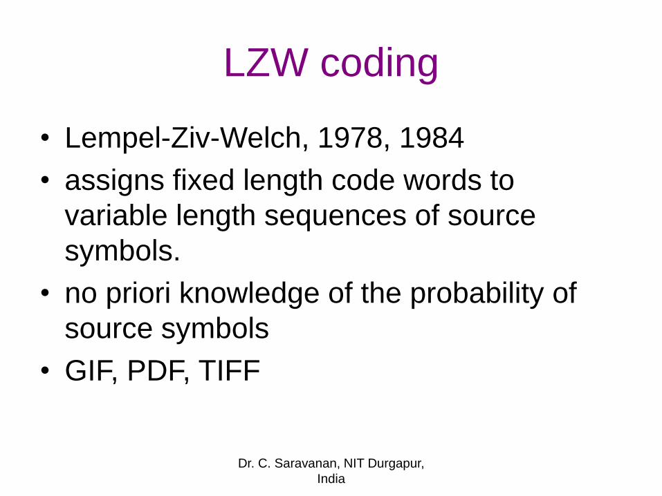
LZW coding

• Lempel-Ziv-Welch, 1978, 1984

• assigns fixed length code words to

variable length sequences of source

symbols.

• no priori knowledge of the probability of

source symbols

• GIF, PDF, TIFF


India

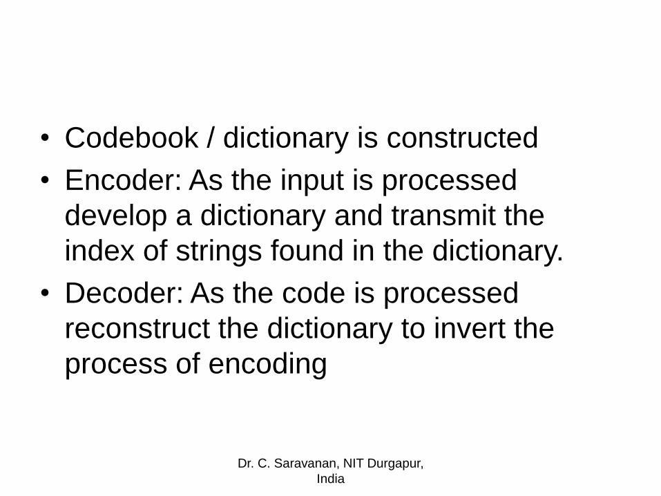
• Codebook / dictionary is constructed

• Encoder: As the input is processed

develop a dictionary and transmit the

index of strings found in the dictionary.

• Decoder: As the code is processed

reconstruct the dictionary to invert the

process of encoding


India

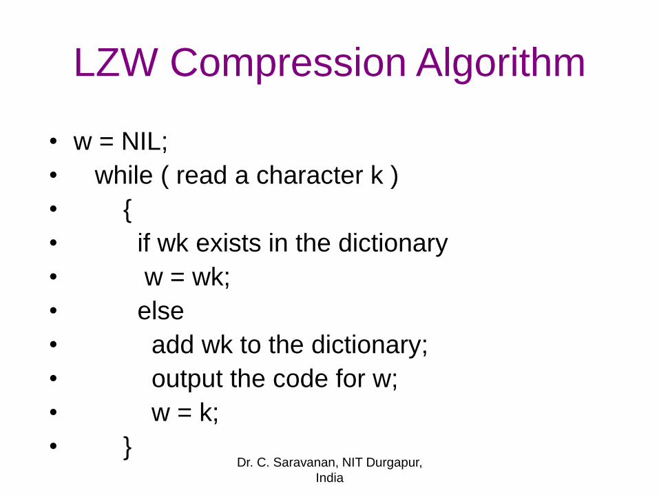
LZW Compression Algorithm

• w = NIL;

• while ( read a character k )

• {

• if wk exists in the dictionary

• w = wk;

• else

• add wk to the dictionary;

• output the code for w;

• w = k;

• }Dr. C. Saravanan, NIT Durgapur,

India

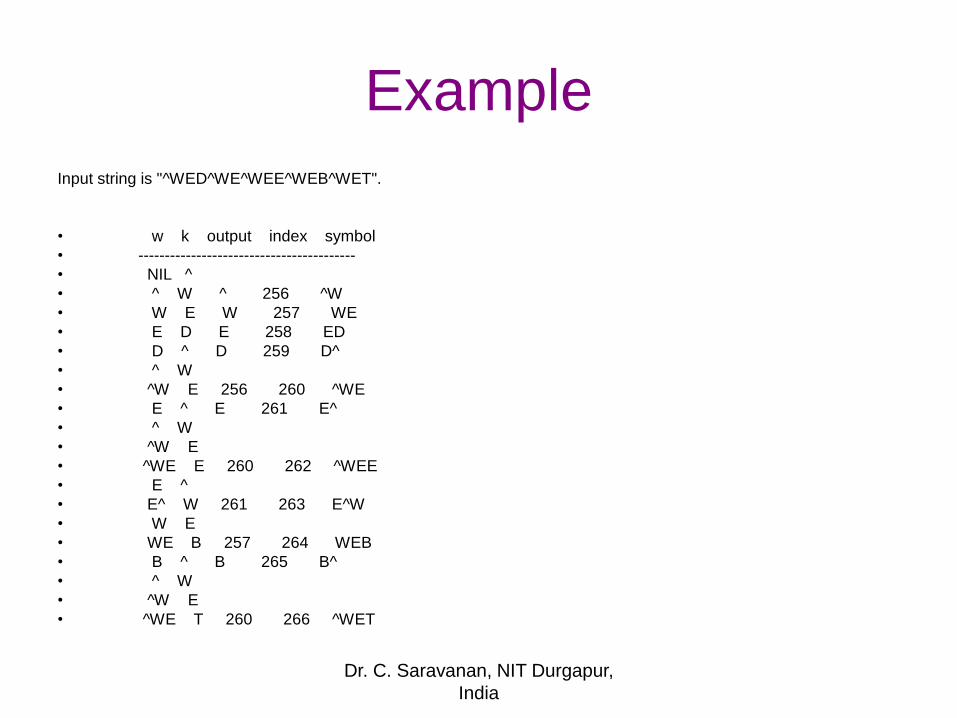
Example

Input string is "^WED^WE^WEE^WEB^WET".

• w k output index symbol

• -----------------------------------------

• NIL ^

• ^ W ^ 256 ^W

• W E W 257 WE

• E D E 258 ED

• D ^ D 259 D^

• ^ W

• ^W E 256 260 ^WE

• E ^ E 261 E^

• ^ W

• ^W E

• ^WE E 260 262 ^WEE

• E ^

• E^ W 261 263 E^W

• W E

• WE B 257 264 WEB

• B ^ B 265 B^

• ^ W

• ^W E

• ^WE T 260 266 ^WET


India

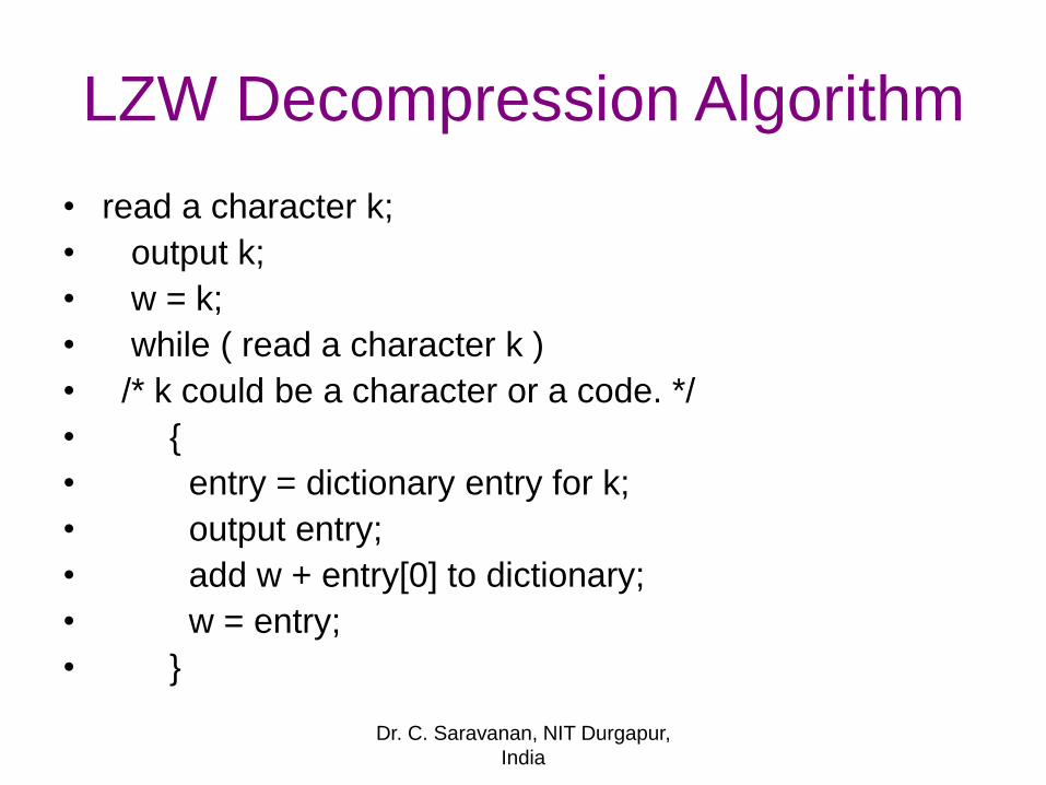
LZW Decompression Algorithm

• read a character k;

• output k;

• w = k;

• while ( read a character k )

• /* k could be a character or a code. */

• {

• entry = dictionary entry for k;

• output entry;

• add w + entry[0] to dictionary;

• w = entry;

• }


India

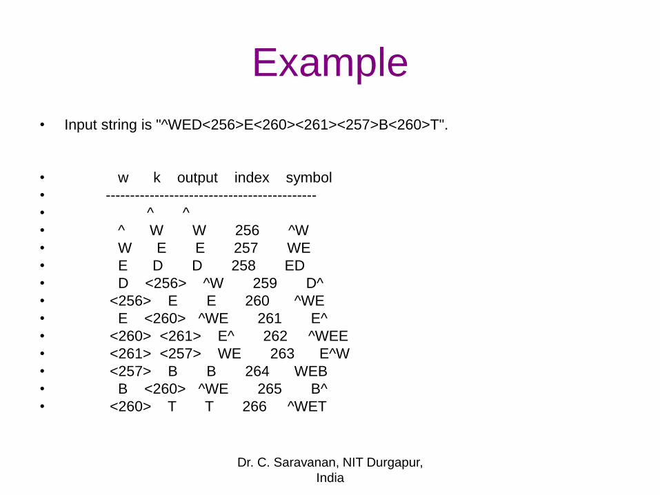
Example

• Input string is "^WED<256>E<260><261><257>B<260>T".

• w k output index symbol

• -------------------------------------------

• ^ ^

• ^ W W 256 ^W

• W E E 257 WE

• E D D 258 ED

• D <256> ^W 259 D^

• <256> E E 260 ^WE

• E <260> ^WE 261 E^

• <260> <261> E^ 262 ^WEE

• <261> <257> WE 263 E^W

• <257> B B 264 WEB

• B <260> ^WE 265 B^

• <260> T T 266 ^WET


India

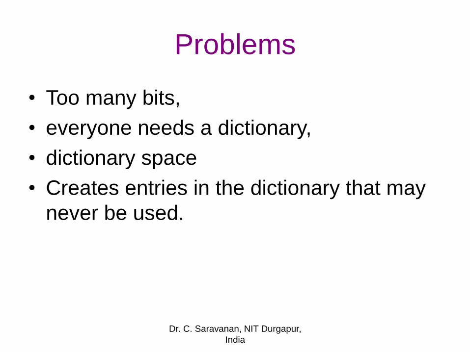
Problems

• Too many bits,

• everyone needs a dictionary,

• dictionary space

• Creates entries in the dictionary that may

never be used.


India

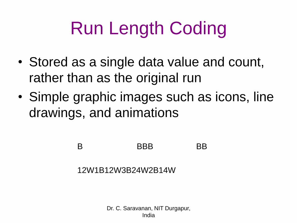
Run Length Coding

• Stored as a single data value and count,

rather than as the original run

• Simple graphic images such as icons, line

drawings, and animations

B BBB BB

12W1B12W3B24W2B14W


India

Example

• consider a screen containing plain

black text on a solid white

background

• There will be many long runs of white

pixels in the blank space, and many

short runs of black pixels within the

text.


India

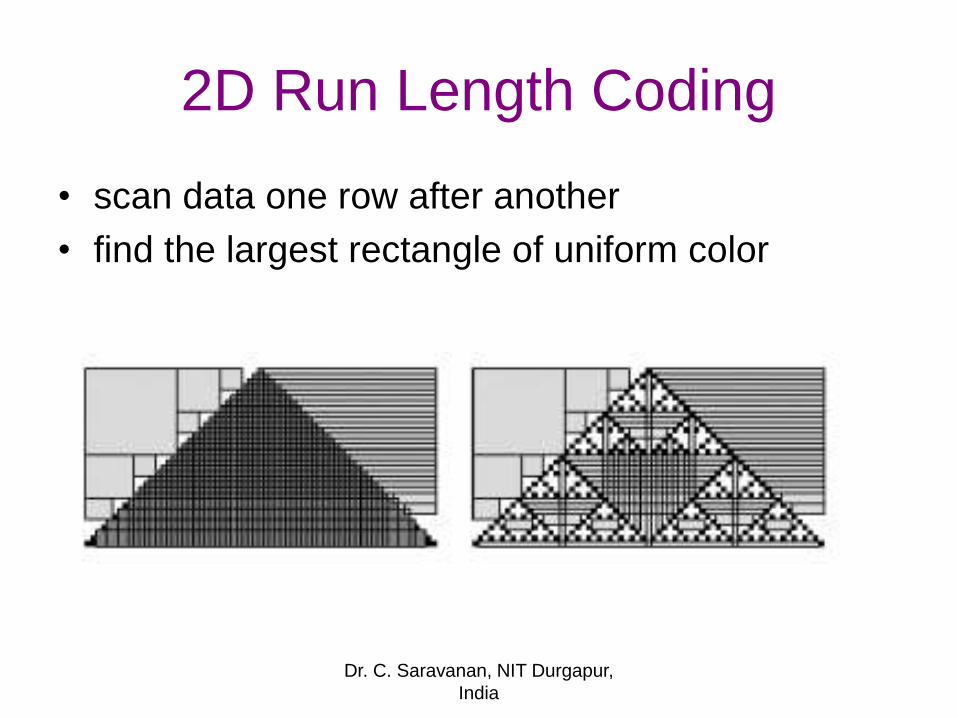
2D Run Length Coding

• scan data one row after another

• find the largest rectangle of uniform color


India

Procedure

• Make a duplicate image matrix

• quantize the colour levels

– reduce the colour levels

– from 256 to 128 / 64 / 32 / 16

– depends on the application reduction level is maintained

– uniform colour level regions are identified

– different colour level regions are labeled and mapped


India

Applications

• Texture Analysis

• Compression

• Segmentation

• Medical Image Analysis

• Layout Analysis

• Text finding, word / line spacings


India

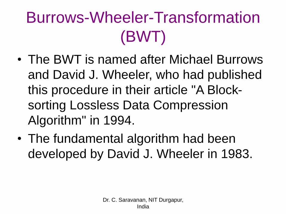
Burrows-Wheeler-Transformation

(BWT)

• The BWT is named after Michael Burrows

and David J. Wheeler, who had published

this procedure in their article "A Block-

sorting Lossless Data Compression

Algorithm" in 1994.

• The fundamental algorithm had been

developed by David J. Wheeler in 1983.


India

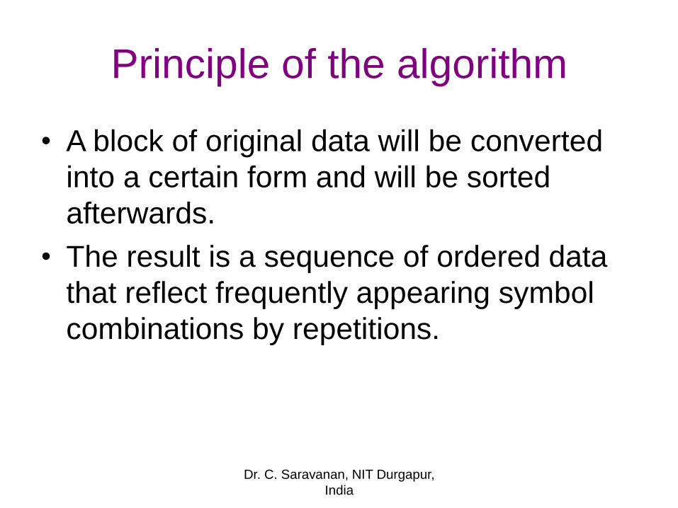
Principle of the algorithm

• A block of original data will be converted

into a certain form and will be sorted

afterwards.

• The result is a sequence of ordered data

that reflect frequently appearing symbol

combinations by repetitions.


India

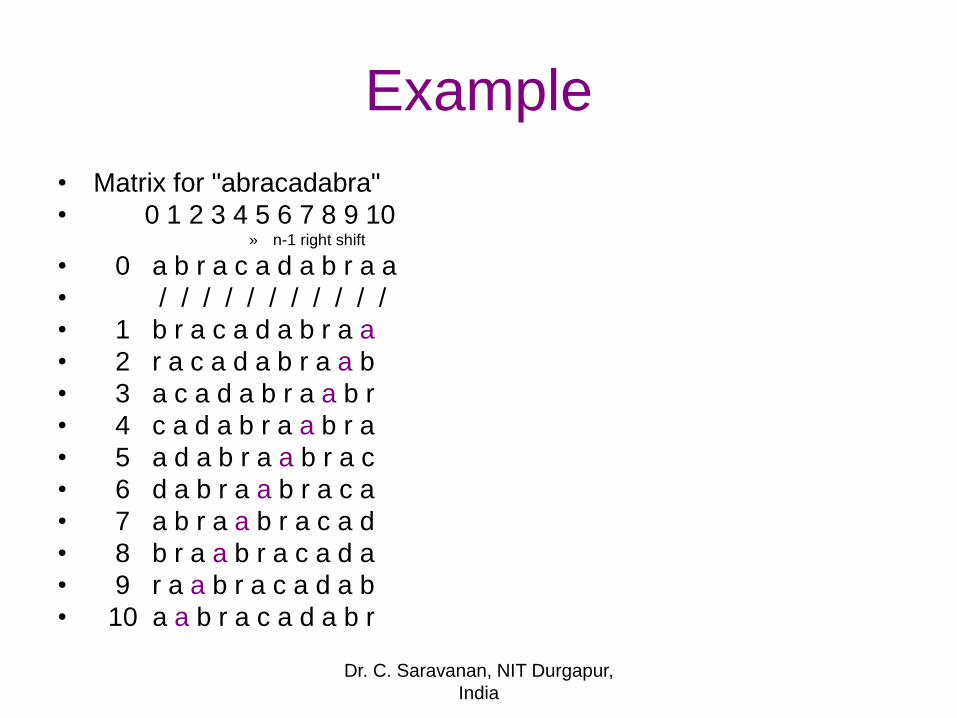
Example

• Matrix for "abracadabra"

• 0 1 2 3 4 5 6 7 8 9 10» n-1 right shift

• 0 a b r a c a d a b r a a

• / / / / / / / / / / /

• 1 b r a c a d a b r a a

• 2 r a c a d a b r a a b

• 3 a c a d a b r a a b r

• 4 c a d a b r a a b r a

• 5 a d a b r a a b r a c

• 6 d a b r a a b r a c a

• 7 a b r a a b r a c a d

• 8 b r a a b r a c a d a

• 9 r a a b r a c a d a b

• 10 a a b r a c a d a b r


India

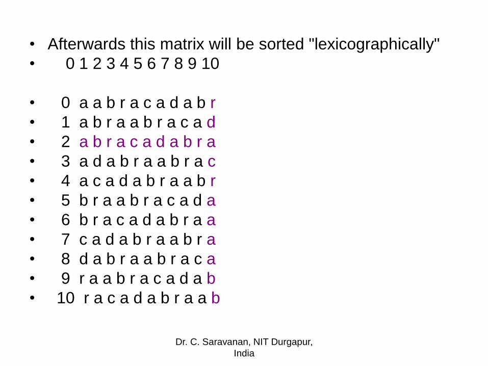
• Afterwards this matrix will be sorted "lexicographically"

• 0 1 2 3 4 5 6 7 8 9 10

• 0 a a b r a c a d a b r

• 1 a b r a a b r a c a d

• 2 a b r a c a d a b r a

• 3 a d a b r a a b r a c

• 4 a c a d a b r a a b r

• 5 b r a a b r a c a d a

• 6 b r a c a d a b r a a

• 7 c a d a b r a a b r a

• 8 d a b r a a b r a c a

• 9 r a a b r a c a d a b

• 10 r a c a d a b r a a b


India

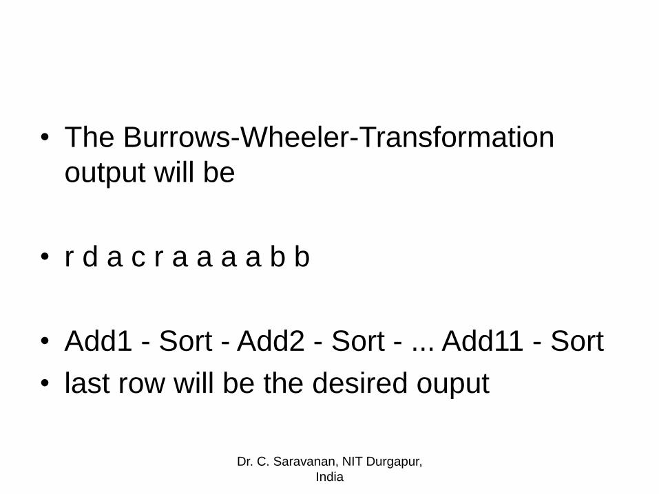
• The Burrows-Wheeler-Transformation

output will be

• r d a c r a a a a b b

• Add1 - Sort - Add2 - Sort - ... Add11 - Sort

• last row will be the desired ouput


India

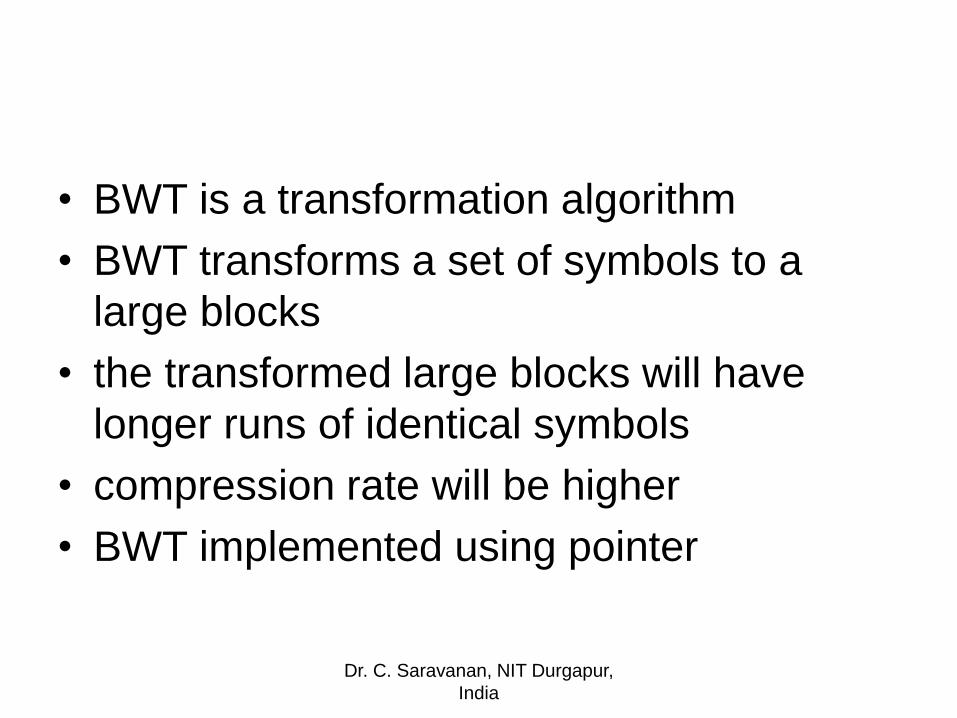
• BWT is a transformation algorithm

• BWT transforms a set of symbols to a

large blocks

• the transformed large blocks will have

longer runs of identical symbols

• compression rate will be higher

• BWT implemented using pointer


India

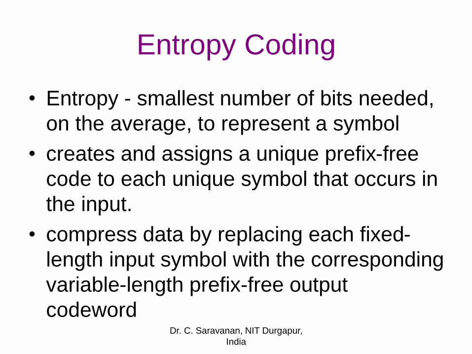
Entropy Coding

• Entropy - smallest number of bits needed,

on the average, to represent a symbol

• creates and assigns a unique prefix-free

code to each unique symbol that occurs in

the input.

• compress data by replacing each fixed-

length input symbol with the corresponding

variable-length prefix-free output

codewordDr. C. Saravanan, NIT Durgapur,

India

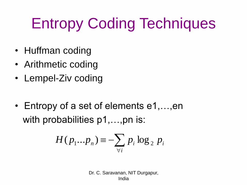
Entropy Coding Techniques

i

iin ppppH 21 log)...(

• Huffman coding

• Arithmetic coding

• Lempel-Ziv coding

• Entropy of a set of elements e1,…,en

with probabilities p1,…,pn is:


India

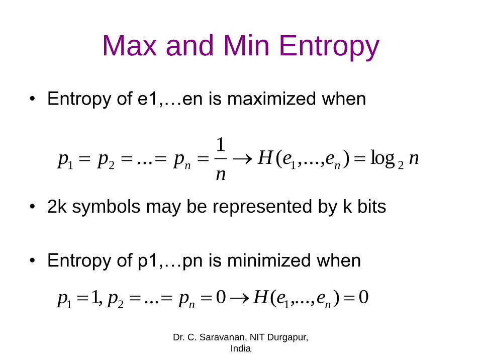
• Entropy of e1,…en is maximized when

• 2k symbols may be represented by k bits

• Entropy of p1,…pn is minimized when

0),...,(0...,1 121 nn eeHppp

Max and Min Entropy

neeHn

ppp nn 2121 log),...,(1

...


India

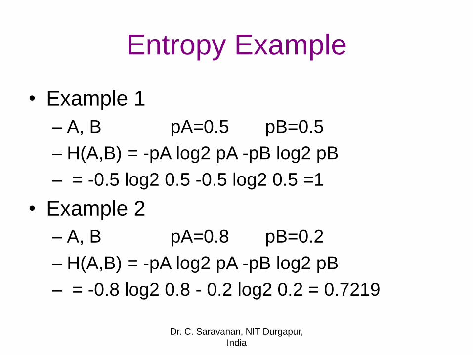
Entropy Example

• Example 1

– A, B pA=0.5 pB=0.5

– H(A,B) = -pA log2 pA -pB log2 pB

– = -0.5 log2 0.5 -0.5 log2 0.5 =1

• Example 2

– A, B pA=0.8 pB=0.2

– H(A,B) = -pA log2 pA -pB log2 pB

– = -0.8 log2 0.8 - 0.2 log2 0.2 = 0.7219


India

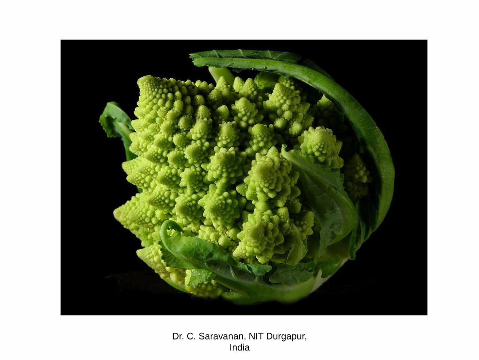
Fractal Compression

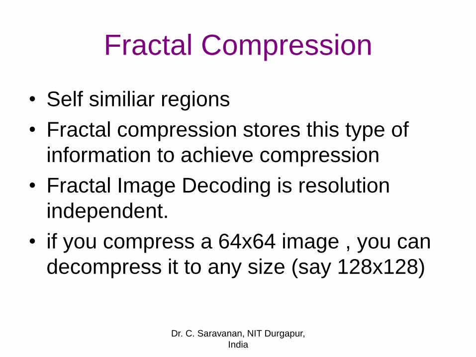
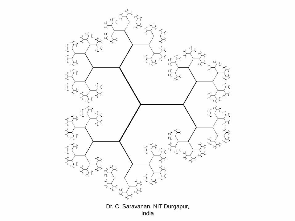
• Self similiar regions

• Fractal compression stores this type of

information to achieve compression

• Fractal Image Decoding is resolution

independent.

• if you compress a 64x64 image , you can

decompress it to any size (say 128x128)


India


India

• Research on fractal image compression evolved in the years 1978-85 using iterated function system (IFS)

• subdivide the image into a partition fixed size square blocks

• then find a matching image portion for each part

• this is known as Partitioned Iterated Function System (PIFS).


India

Challenges

• how should the image be segmented,

• where should one search for matching

image portions,

• how should the intensity transformation

bedesigned


India

Four views of fractal image

compression

1. Iterated function systems (IFS)

– operators in metric spaces (metric space is a set for which

distances between all members of the set are defined)

2. Self vector quantization

– 4 x 4 blocks - code book

3. Self-quantized wavelet subtrees

– organize the (Haar) wavelet coefficients in a tree and to

approximate subtrees by scaled copies of other subtrees closer

to the root of the wavelet tree

4. Convolution transform coding

– convolution operation used for finding matching regions


India


India

Digital Watermarking

• "digital watermark" was first coined in

1992 by Andrew Tirkel and Charles

Osborne.

• First watermarks appeared in Italy during

the 13th century

• Watermarks are hiding identification marks

produced during the paper making

process


India

• process of hiding digital information in a image / audio / video.

• identify ownership / copyright of image / audio / video.– copy right infringements

– banknote authentication

– pirated movie - source tracking

– broadcast monitoring


India

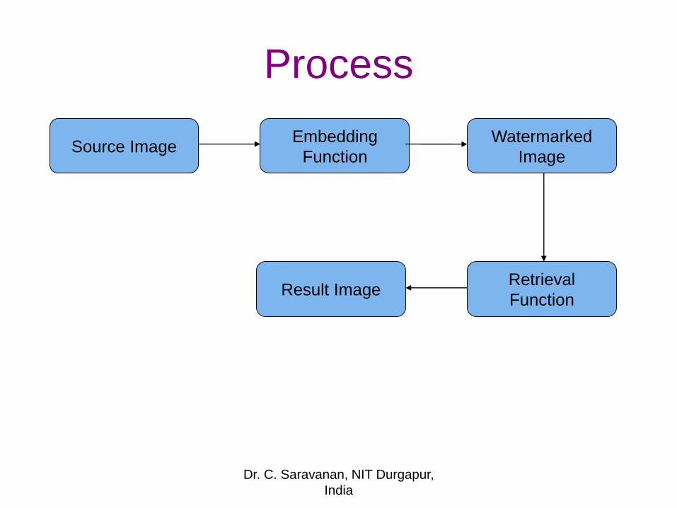
Process

Source ImageEmbedding

Function

Watermarked

Image

Retrieval

FunctionResult Image


India

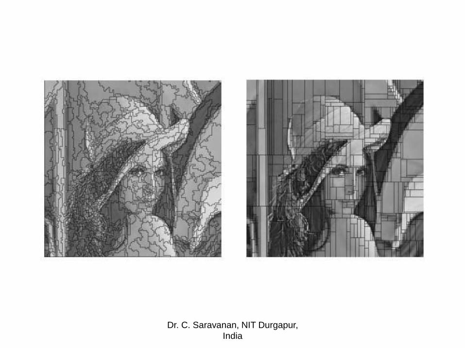
Visible Watermark


India

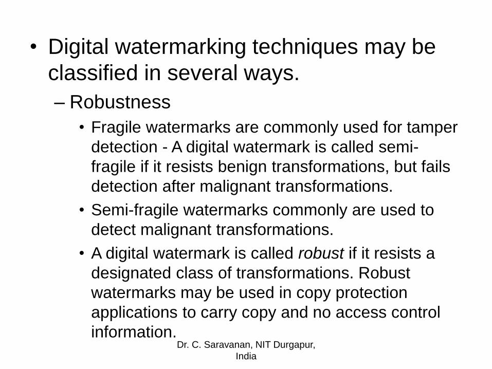
• Digital watermarking techniques may be

classified in several ways.

– Robustness

• Fragile watermarks are commonly used for tamper

detection - A digital watermark is called semi-

fragile if it resists benign transformations, but fails

detection after malignant transformations.

• Semi-fragile watermarks commonly are used to

detect malignant transformations.

• A digital watermark is called robust if it resists a

designated class of transformations. Robust

watermarks may be used in copy protection

applications to carry copy and no access control

information.Dr. C. Saravanan, NIT Durgapur,

India

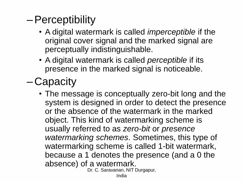
– Perceptibility• A digital watermark is called imperceptible if the

original cover signal and the marked signal are perceptually indistinguishable.

• A digital watermark is called perceptible if its presence in the marked signal is noticeable.

– Capacity• The message is conceptually zero-bit long and the

system is designed in order to detect the presence or the absence of the watermark in the marked object. This kind of watermarking scheme is usually referred to as zero-bit or presence watermarking schemes. Sometimes, this type of watermarking scheme is called 1-bit watermark, because a 1 denotes the presence (and a 0 the absence) of a watermark.


India

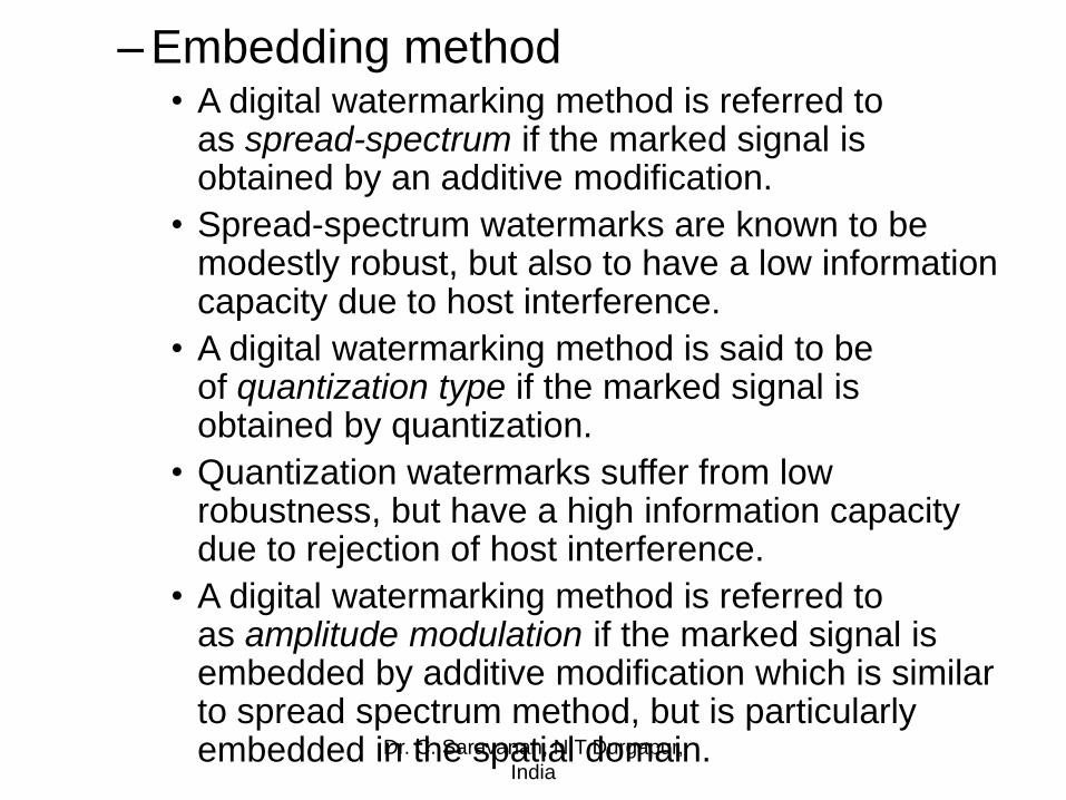
– Embedding method• A digital watermarking method is referred to

as spread-spectrum if the marked signal is obtained by an additive modification.

• Spread-spectrum watermarks are known to be modestly robust, but also to have a low information capacity due to host interference.

• A digital watermarking method is said to be of quantization type if the marked signal is obtained by quantization.

• Quantization watermarks suffer from low robustness, but have a high information capacity due to rejection of host interference.

• A digital watermarking method is referred to as amplitude modulation if the marked signal is embedded by additive modification which is similar to spread spectrum method, but is particularly embedded in the spatial domain.Dr. C. Saravanan, NIT Durgapur,

India

Models

• Communication based models

– The sender would encode a message using

some kind of encoding key to prevent

eavesdroppers to decode the message. Then

the message would be transmitted on a

communications channel. At the other end of

the transmission by the receiver, try to decode

it using a decoding key, to get the original

message back.


India

• Geometric models

– watermarked and unwatermarked, can be

viewed as high-dimensional vectors

– Geometric Watermarking process consists of

several regions.

– The embedding region, which is the region

that contains all the possible images resulting

from the embedding of a message inside an

unwatermarked image using some watermark

embedding algorithm.Dr. C. Saravanan, NIT Durgapur,

India

– Another very important region is the detection

region, which is the region containing all the

possible images from which a watermark can

be successfully extracted using a watermark

detection algorithm.


India

• http://hal.inria.fr/docs/00/08/42/68/PDF/ch

apter7.pdf

• https://www.cl.cam.ac.uk/teaching/0910/R

08/work/essay-ma485-watermarking.pdf


India

http://hal.inria.fr/docs/00/08/42/68/PDF/chapter7.pdf

https://www.cl.cam.ac.uk/teaching/0910/R08/work/essay-ma485-watermarking.pdf

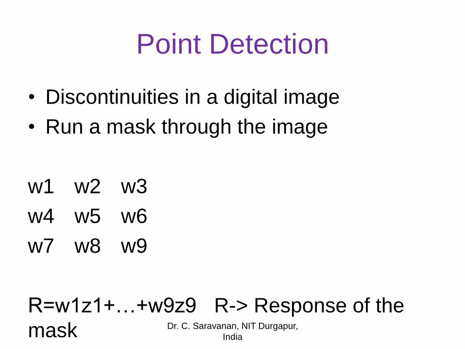
Point Detection

• Discontinuities in a digital image

• Run a mask through the image

w1 w2 w3

w4 w5 w6

w7 w8 w9

R=w1z1+…+w9z9 R-> Response of the

mask Dr. C. Saravanan, NIT Durgapur,

India

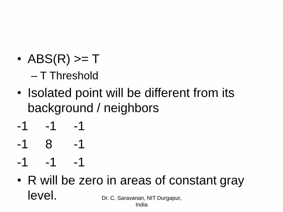
• ABS(R) >= T

– T Threshold

• Isolated point will be different from its

background / neighbors

-1 -1 -1

-1 8 -1

-1 -1 -1

• R will be zero in areas of constant gray

level. Dr. C. Saravanan, NIT Durgapur,

India

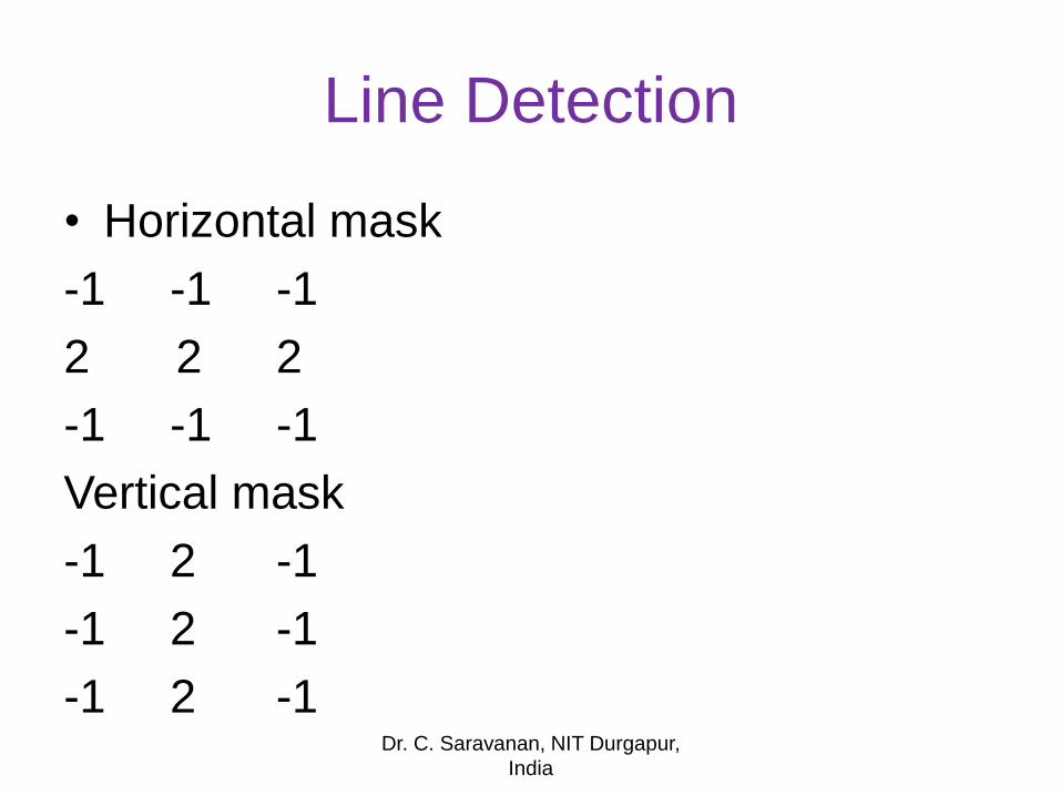
Line Detection

• Horizontal mask

-1 -1 -1

2 2 2

-1 -1 -1

Vertical mask

-1 2 -1

-1 2 -1

-1 2 -1Dr. C. Saravanan, NIT Durgapur,

India

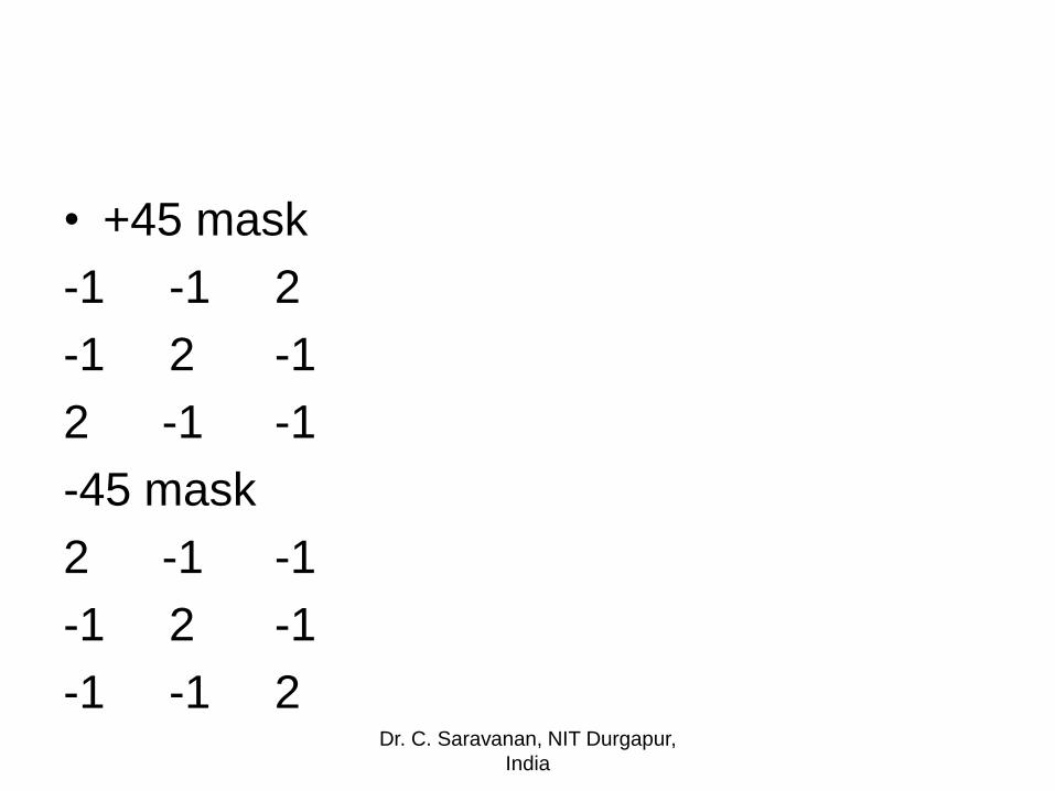
• +45 mask

-1 -1 2

-1 2 -1

2 -1 -1

-45 mask

2 -1 -1

-1 2 -1

-1 -1 2Dr. C. Saravanan, NIT Durgapur,

India

• Four masks run individually through an

image,

• At an certain point Abs(Ri) > Abs(Rj) for all

j not equal i,

• That point is said to be more likely

associated with a line in the direction of

the mask i.


India

Edge Detection

• Meaningful discontinuities

• First and second order digital derivative

approaches are used

• Edge is a set of connected pixels that lie

on the boundary between two regions


India

Segmentation

• Classified into

– Edge based

– Region based

– Data clustering


India

Any Questions ?


India

References

Computer Vision: A Modern Approach by David Forsyth and Jean Ponce

Computer Vision: Algorithms and Applications by Richard Szeliski's

Computer Vision: Detection, Recognition and Reconstruction

En.wikipedia.org

in.mathworks.com

imagej.net


India

Computer vision

Education

Transcript of Computer vision