Computer Science & Information Technology 24 › csit › csit424.pdf · 2016-11-25 · Lokesh Kr....
77
Computer Science & Information Technology 24
Transcript of Computer Science & Information Technology 24 › csit › csit424.pdf · 2016-11-25 · Lokesh Kr....

Computer Science &
Information Technology 24


Natarajan Meghanathan
Jan Zizka (Eds)
Computer Science &
Information Technology
Third International conference on Advanced Computer Science and
Information Technology (ICAIT 2014)
Sydney, Australia, July 12 ~ 13 - 2014
AIRCC
Volume Editors
Natarajan Meghanathan,
Jackson State University, USA
E-mail: [email protected]
Jan Zizka,
Mendel University in Brno, Czech Republic
E-mail: [email protected]
ISSN : 2231 - 5403
ISBN : 978-1-921987-20-5
DOI : 10.5121/csit.2014.4701 - 10.5121/csit.2014.4707
This work is subject to copyright. All rights are reserved, whether whole or part of the material is
concerned, specifically the rights of translation, reprinting, re-use of illustrations, recitation,
broadcasting, reproduction on microfilms or in any other way, and storage in data banks.
Duplication of this publication or parts thereof is permitted only under the provisions of the
International Copyright Law and permission for use must always be obtained from Academy &
Industry Research Collaboration Center. Violations are liable to prosecution under the
International Copyright Law.
Typesetting: Camera-ready by author, data conversion by NnN Net Solutions Private Ltd.,
Chennai, India

Preface
Third International conference on Advanced Computer Science and Information Technology (ICAIT
2014) was held in Sydney, Australia, during July 12~13, 2014. Third International Conference on
Digital Image Processing and Vision (ICDIPV 2014), Third International Conference on Information
Technology Convergence and Services (ITCSE 2014), Second International Conference of Networks
and Communications (NC 2014) were collocated with the ICAIT-2014. The conferences attracted
many local and international delegates, presenting a balanced mixture of intellect from the East and
from the West.
The goal of this conference series is to bring together researchers and practitioners from academia and
industry to focus on understanding computer science and information technology and to establish new
collaborations in these areas. Authors are invited to contribute to the conference by submitting articles
that illustrate research results, projects, survey work and industrial experiences describing significant
advances in all areas of computer science and information technology.
The ICAIT-2014, ICDIPV-2014, ITCSE-2014, NC-2014 Committees rigorously invited submissions
for many months from researchers, scientists, engineers, students and practitioners related to the
relevant themes and tracks of the workshop. This effort guaranteed submissions from an unparalleled
number of internationally recognized top-level researchers. All the submissions underwent a strenuous
peer review process which comprised expert reviewers. These reviewers were selected from a talented
pool of Technical Committee members and external reviewers on the basis of their expertise. The
papers were then reviewed based on their contributions, technical content, originality and clarity. The
entire process, which includes the submission, review and acceptance processes, was done
electronically. All these efforts undertaken by the Organizing and Technical Committees led to an
exciting, rich and a high quality technical conference program, which featured high-impact
presentations for all attendees to enjoy, appreciate and expand their expertise in the latest
developments in computer network and communications research.
In closing, ICAIT-2014, ICDIPV-2014, ITCSE-2014, NC-2014 brought together researchers,
scientists, engineers, students and practitioners to exchange and share their experiences, new ideas and
research results in all aspects of the main workshop themes and tracks, and to discuss the practical
challenges encountered and the solutions adopted. The book is organized as a collection of papers
from the ICAIT-2014, ICDIPV-2014, ITCSE-2014, NC-2014.
We would like to thank the General and Program Chairs, organization staff, the members of the
Technical Program Committees and external reviewers for their excellent and tireless work. We
sincerely wish that all attendees benefited scientifically from the conference and wish them every
success in their research. It is the humble wish of the conference organizers that the professional
dialogue among the researchers, scientists, engineers, students and educators continues beyond the
event and that the friendships and collaborations forged will linger and prosper for many years to
come.
Natarajan Meghanathan
Jan Zizka

Organization
Program Committee Members
Abd El-Aziz Ahmed Anna's University, Egypt
Abdellah Idrissi Computer Science Laboratory (LRI), Rabat
Abdurrahman Celebi Beder University, Albania
Abhijit Das RCC Institute of Information Technology, India
Aiden B Lee Qualcomm Inc, USA
Akanksha Joshi CDAC, India
Alaa Y. Taqa University of Mosul, Iraq
Ali Elkateeb University of Michigan-Dearborn, USA
Alireza Pourebrahimi I.A.U., E-campus, Iran
Amine Achouri University of Tunis, Tunisia
Amir Salarpour Bu-Ali Sina University, Iran.
Ammar Odeh University of Bridgeport, USA
Anamika Ahirwar Rajiv Gandhi Technical University, India
Anuradha S SVPCET, India
Arash Habibi Lashkari University Technology of Malaysia, Malaysia
Asadollah Shahbahrami University of Guilan, Iran
Asha K. Krupanidhi School of Management, India
Ayad Ghany Ismaeel Hawler Polytechnic University, Iraq
Ben Ahmed M. Abdelmalek Essaasi University, Morocco
Berlin Hency V. Madras Institute of Technology, India
Bhadeshiya Jaykumar R Gujarat Technological University, India
Bhaskar Biswas Banaras Hindu University,India
Brijender Kahanwal Galaxy Global Group of Institutions, India
Chanabasayya Vastrad Mangalore University, India
Chandan Kapoor Chitkara University, India
Chandramohan B Anna University, India
Chenna Reddy P JNTUA College of Engineering, India
Chithik Raja M. Salalah College of Technology, Oman
Dac-Nhuong Le Haiphong University, Vietnam
Daniel K. M.M.M University of Technology, India
Derya Birant Dokuz Eylul University, Turkey
Dhinaharan Nagamalai Wireilla Net Solutions, Australia
Dongchen Li Peking University, P.R.China
Durgesh Samadhiya Chung Hua University, Taiwan
Ekata Mehul Semiconductor Services, India
Ekram Khan Aligarh Muslim University, India
El Miloud Ar reyouchi Abdelmalek Essaadi university, Morroco
Elboukhari Mohamed Unviersity Mohamed First, Morocco
El-Mashad Wageningen University, Netherland
Farhad Soleimanian Gharehchopogh Hacettepe University, Turkey
Farzad Kiani İstanbul S.Zaim University, Turkey
Fasil Fenta University of Gondar, Ethiopia

Fatemeh Alidusti Islamic Azad University, Iran
Florin Balasa The American University, Cairo
Francisca N. Ogwueleka Federal University Wukari, Nigeria
Ganga Rama Koteswara Rao V.R Siddhartha Engineering College, India
Garje Goraksh V PVG's College of Engg. & Tech, India
Geetha Ramani Anna University, India
Geetha S BIT Campus, India
Girija Chetty University of Canberra, Australia
Gomathy C SRM University, India
Govinda K. VIT University, India
Gulista Khan Teerthanker Mahaveer University, India
Hamdi Yalin Yalic Hacettepe University, Turkey
Hashem Rahimi Zand Institute, Iran
Hossein Jadidoleslamy MUT University, Iran
Inderveer Chana Thapar University, India
Ingole, Piyush K. Raisoni Group of Institutions,India
Isa Maleki Islamic Azad University, Iran
Jagadeesha M Dilla University, Ethiopia
Jan Zizka Mendel University in Brno, Czech Republic
Janani Rajaraman SCSVMV University, India
Jitendra Maan Tata Consultancy Services, India
Jobin Christ M.C Adhiyamaan College of Engineering, India
John Tengviel Sunyani Polytechnic, Ghana
Kamal Ghoumid PR Mohamed Premier University, Morroco
Kanaka Rao P.V. Dilla University, Ethiopia
Kanti Prasad University of Massachusetts Lowell, USA
Karthikeyan S. Sathyabama University,India
Khalifa A. Zaied Mansoura University, Egypt
Koushik Majumder West Bengal University of Technology, India
Krishna Prasad P.E.S.N, Prasad V. Potluri Siddhartha Institute of
Technology, India
Kulkarni P J Walchand College of Engineering, India
Lokesh Kr. Bansal I.T.S. Engineering College, India
Mahesh P.K Don Bosco Institute of Technology, India
Mahesha P S J College of Engineering, India
Manal King Abdulaziz University KAU, Saudi Arabia
Maninder Singh Thapar University,India
Manish T I MET's School of Engineering, India
Manjunath T.C HKBK College of Engineering, India
Manoranjini J Tagore Engineering College, India
Mansaf Alam Jamia Millia Islamia, India
Mantosh Biswas National Institute of Technology, India
Marish Kumar GNIT, India
Martínez-Zarzuela Mario University of Valladolid, Spain
Md Firoj Ali Aligarh Muslim University, India
Meenakshi A.V Periyar Maniammai University, India
Meyyappan Alagappa University, India
Minu R.I. Jerusalem College of Engineering, India

Mohammad Zunnun Khan Integral University, India
Mohammed Ali Hussain KL University, India
Mohd Umar Farooq Osmania University, India
Mrinal Kanti Debbarma NIT - Agartala, India
Muhammad Asif Manzoor Umm Al-Qura University, Saudi Arabia
Muhammad Naufal Mansor University Malaysia Perlis, Malaysia
Nag SV RMK Engineering College, India
Narayanan Sundararajan Alagappa University, India
Naresh Sharma SRM University, India
Natarajan Meghanathan Jackson State University, USA
Neetesh Saxena IIT Indore, India
Nilesh Ranpura Semiconductor Services, India
Nilima Salankar Sir Padampat Singhania University, India
Niloofar Khanghahi Islamic Azad University, Iran
Osama Hourani Tarbiat Modares University, Iran
Padmaja M VR Siddhartha Engg College, India
Padmavathi S Amrita School of Engineering, India
Palaniswami M The University of Melbourne, Australia
Palson Kennedy R Anna University, India
Parveen Sharma Himachal Stated & Listed of UGC., India
Philomina Simon University of Kerala, India
Prabhu P Alagappa University, India
Pradeepa.N SNS College of Technology, India
Pradnya Kulkarni Federation University, Australia
Prasad T. V Visvodaya Technical Academy, Kavali, India
Pushpendra Pateriya Lovely Professional University, India
Radha V Avinashilingam University, India
Rafah M. Almuttairi University of Babylon, Iraq
Raj Mohan R IFET College of Engineering, India
Rajan Vohra Guru Nanak Dev University, India
Rajani Kanth T V SNIST, India
Rajib Kumar Jha Indian Institute of Technology Patna, India
Ramasubramanian Syed Ammal Engineering College, India
Ramesh Babu K VIT University, India
Ramgopal Kashyap Sagar Institute of Science and Technology, India
Ramkumar Prabhu M Anna University, India
Ranjeet Vasant Bidwe PICT, India
Rasmiprava singh MATS University, India
Ravendra Singh MJP Rohilkhand University, India
Ravi sahankar Yadav Centre for AI & Robotics, India
Ravilla Dilli Manipal University, India
Ripal Patel BVM Engineering College, India
Ritu Chauhan Amity University,India
Sachidananda Biju Patnaik University of Technology, India
Sachin Kumar IIT Roorkee, India
SaeidMasoumi Malek-Ashtar University of Technology, Iran
Saikumar T CMR Technical Campus, India
Sameer S M NIT, India

Samitha Khaiyum Dayananda Sagar College of Engineering, India
Sandhya Tarar School of ICT, India
Sangita Zope-Chaudhari A. C. Patil College of Engineering, India
Sangram Ray Indian School of Mines, India
Sanjay Singh Manipal Institute of Technology, India
Sanjeev Puri SRMGPC, India
Sanjiban Sekhar Roy VIT University, India
Sanjoy Das Galgotias University, India
Sankara Malliga G Dhanalakshmi College of Engineering, India
Santosh Naik Jain University, India
Sasirekha N Rathinam College of Arts and Science, India
Satria Mandala Universiti Teknologi Malaysia, Malaysia
Satyaki Roy St. Xavier's College, India
Seyed Ziaeddin Alborzi Nanyang Technologcal University, Singapore
Seyyed Reza Khaze Islamic Azad University, Iran
Shankar D. Nawale Sinhgad Institute of Technology, India
Shanthi Selvaraj Anna University, India
Sharma M.K Uttarakhand Technical University, India
Sharvani.G.S R V College of Engineering, Bangalore, India
Shivaprakasha K S Bahubali College of Engineering, India
Shrikant Tiwari Shri Shankaracharya Technical Campus, India
Sonam Mahajan Thapar University, India
Sornam M University of Madras, India
Soumen Kanrar Vehere Interactive (P) Ltd, India
Sridevi S Sethu Institute of Technology, India
Srinath N. K R.V. College of Engineering, India
Suma.S Bhartiyar university, India
Sumit Chaudhary Shri Ram Group of Colleges, India
Sumithra devi R.V.College of engineering, India
Sundarapandian Vaidyanathan Vel Tech University, India
Suprativ Saha Adamas Institute of Technology, India
Supriya Chakraborty JIS College of Engineering, India
Surekha Mariam Varghese M.A.College of Engineering, India
Suresh Kumar Manav Rachna International University, India
Sutirtha K Guha Seacom Engineering College, India
Syed Abdul Sattar Royal Institute of Technology & Science, India
TTaruna S Banasthali University, Iindia
Thaier Hayajneh The Hashemite University, Jordan
Thomas Yeboah Christian Service University, Ghana
Trisiladevi C. Nagavi S J College of Engineering, India
Tunisha Shome Samsung India, India
Uma Rani R Sri Sarada College for Women, India
Urmila Shrawankar GHRCE ,India
Usha Jayadevappa R.V. College of Engineering, India
Vadivel M Sethu Institute of Technology, India
Valliammal N Avinashilingam University for Women, India
Varadala Sridhar Vidya Jyothi Institute of Technology, India
Veena Gulhane G.H.Raisoni College of Engg ,India

Venkata Narasimha Inukollu Texas Tech University, USA
Vidya Devi V M.S. Engineering college, India
Vijayakumar P Anna University, India
William R Simpson The Institute for Defense Analyses, USA
Xavier Arputha Rathina B.S.Abdur Rahman University, India
Xinilang Zheng Frostburg State University, USA
Yassine Ben Ayed Sfax University, Tunisia
Yazdan Jamshidi Islamic Azad University, Iran
Yousef El Mourabit IBN ZOHR University, Morocco
Zahraa Al Zirjawi Isra University, Jordan
Zeinab Abbasi Khalifehlou Islamic Azad University, Iran
Zhang Xiantao Peking University, P.R.China
Zuhal Tanrikulu Bogazici University, Turkey
Technically Sponsored by
Computer Science & Information Technology Community (CSITC)
Networks & Communications Community (NCC)
Digital Signal & Image Processing Community (DSIPC)
Organized By
ACADEMY & INDUSTRY RESEARCH COLLABORATION CENTER (AIRCC)

TABLE OF CONTENTS
Third International conference on Advanced Computer Science and
Information Technology (ICAIT 2014)
Hardware Complexity of Microprocessor Design According to Moore's Law.. 01 - 07
Haissam El-Aawar
Using Grid Puzzle to Solve Constraint-Based Scheduling Problem………...… 09 - 18
Noppon Choosri
A Theoretical Framework of the Influence of Mobility in Continued
Usage Intention of Smart Mobile Device……………………...……..………...… 19 - 26
Vincent Cho and Eric Ngai
Third International Conference on Digital Image Processing and Vision
(ICDIPV 2014 )
Wavelet-Based Warping Technique for Mobile Devices…………...………...… 27 - 34
Ekta Walia and Vishal Verma
Adaptive Trilateral Filter for In-Loop Filtering………..…………..………...… 35 - 41
Akitha Kesireddy and Mohamed El-Sharkawy
Third International Conference on Information Technology
Convergence and Services (ITCSE 2014)
A Cloud Service Selection Model Based on User-Specified Quality of
Service Level…………………………………………………………..………...… 43 - 54
Chang-Ling Hsu
Second International Conference of Networks and Communications
(NC 2014 )
Performance Evaluation of a Layered WSN Using AODV and MCF
Protocols in NS-2…………………………………….………………..………...… 55 - 65
Apoorva Dasari and Mohamed El-Sharkawy
Natarajan Meghanathan et al. (Eds) : ICAIT, ICDIPV, ITCSE, NC - 2014
pp. 01–07, 2014. © CS & IT-CSCP 2014 DOI : 10.5121/csit.2014.4701
HARDWARE COMPLEXITY OF
MICROPROCESSOR DESIGN ACCORDING
TO MOORE’S LAW
Haissam El-Aawar
Associate Professor, Computer Science/Information Technology Departments
Lebanese International University – LIU, Bekaa – Lebanon [email protected], [email protected]
ABSTRACT
The increasing of the number of transistors on a chip, which plays the main role in improvement
in the performance and increasing the speed of a microprocessor, causes rapidly increasing of
microprocessor design complexity. Based on Moore’s Law the number of transistors should be
doubled every 24 months. The doubling of transistor count affects increasing of microprocessor
design complexity, power dissipation, and cost of design effort.
This article presents a proposal to discuss the matter of scaling hardware complexity of a
microprocessor design related to Moore’s Law. Based on the discussion a hardware complexity
measure is presented.
KEYWORDS
Hardware Complexity, Microprocessor Design, Transistor Count, Die Size, Density.
1. INTRODUCTION
Algorithms’ Complexity is regarded as one of the significant measurement, which is appearing
along the recent past. Although, there is a rapid development in the algorithmic devices, which
involve a computer system as one of their examples; complexity is still occupying a major role in
computer design, if it is thought to be oriented towards the hardware or software view [1, 2].
The development of IC technology and design has been characterized by Moore’s Law during the
past fifty years. Moore’s Law states that the transistor count on a chip would double every two
years [3, 4]; applying Moore’s law in the design of the microprocessors makes it more
complicated and more expensive. To fit more transistors on a chip, the size of the chip must be
increasing and/or the size of the transistors must be decreasing. As the feature size on the chip
goes down, the number of transistors rises and the design complexity also rises.
Microprocessor design has been developed by taking into consideration the following
characteristics: performance, speed, design time, design complexity, feature size, die area and
others. These characteristics are generally interdependent. Increasing the number of transistors
raises the die size, the speed and the performance of a microprocessor; more transistors, more
clock cycles. Decreasing the feature size increases the transistor count, the design complexity and
the power dissipation [5, 6].
2 Computer Science & Information Technology (CS & IT)
2. HARDWARE COMPLEXITY MEASUREMENT Hardware complexity measurement is used to scale the number of elements, which are
compounded, along any selected level of hardware processing. Any selected level, includes all the
involved structures of hardware appearing beyond a specific apparatus. The hardware complexity
measurement id defined as:
A = | E | (1)
where, E is the multitude of the elements emerging in a hierarchal structural diagram.
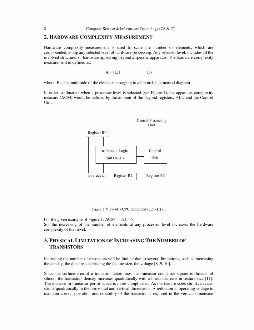
In order to illustrate when a processor level is selected (see Figure.1), the apparatus complexity measure (ACM) would be defined by the amount of the beyond registers, ALU and the Control
Unit.
Figure.1.View of a CPU complexity Level, [7].
For the given example of Figure.1: ACM = | E | = 6.
So, the increasing of the number of elements at any processor level increases the hardware
complexity of that level.
3. PHYSICAL LIMITATION OF INCREASING THE NUMBER OF
TRANSISTORS
Increasing the number of transistors will be limited due to several limitations, such as increasing
the density, the die size, decreasing the feature size, the voltage [8, 9, 10].
Since the surface area of a transistor determines the transistor count per square millimeter of
silicon, the transistors density increases quadratically with a linear decrease in feature size [11].
The increase in transistor performance is more complicated. As the feature sizes shrink, devices
shrink quadratically in the horizontal and vertical dimensions. A reduction in operating voltage to
maintain correct operation and reliability of the transistor is required in the vertical dimension
Register R1 Register R2 Register R3
Arithmetic-Logic
Unit (ALU)
Control
Unit
Central Processing
Unit
Register R0

Computer Science & Information Technology (CS & IT) 3
shrink. This combination of scaling factors leads to a complex interrelationship between the
transistor performance and the process feature size.
Due to the shrinking of the pixel size and the increasing of the density, the hardware complexity
raises. If the pixel size shrinks double and the density increases double every two years according
to Moore’s Law, the physical limitation will definitely appear in few years, which means that it
will be very difficult to apply Moore’s Law in the future. Some studies have shown that physical
limitations could be reached by 2018 [12] or 2020-2022[13, 14, 15, 16].
Applying Moore’s Law by doubling the number of transistors every two years increases the speed
and performance of the processor and causes increasing the processor’s hardware complexity (see
Table 1), which will be limited after a few years [17, 18, 19, 20].
Table 1. Complexity Of microchip And Moore’s Law
Year Microchip Complexly Transistors
Moore’s Law:
Complexity: Transistors
1959 1 20 = 1
1964 32 25 = 32
1965 64 26 = 64
1975 64,000 216 = 64,000
Table 2 shows the apparatus complexity measurement of different microprocessors from 1971 till 2012.
Table 2. Evolution of Microprocessors And Apparatus Complexity Measurement: 1971 to 2012
Manufacturer Processor Date of introduction
Number of transistors (Apparatus Complexity)
Area [mm
2]
Intel
Intel4004 1971 2,300 12
Intel8008 1972 3,500 14
Intel8080 1974 4,400 20
Intel8085 1976 6,500 20
Intel8086 1978 29,000 33
Intel80286 1982 134,000 44
Intel80386 1985 275,000 104
Intel80486 1989 1,180,235 173
Pentium 1993 3,100,000 294
Pentium Pro 1995 5,500,000 307
Pentium II 1997 7,500,000 195
Pentium III 1999 9,500,000 128
Pentium 4 2000 42,000,000 217
Itanium 2 McKinely
2002 220,000,000 421

4 Computer Science & Information Technology (CS & IT)
Core 2 Duo 2006 291,000,000 143
Core i7 (Quad) 2008 731,000,000 263
Six-Core Core i7
2010 1,170,000,000 240
Six-Core Core i7/8-Core Xeon E5
2011 2,270,000,000 434
8-Core Itanium Poulson
2012 3,100,000,000 544
MIPS
R2000 1986 110,000 80
R3000 1988 150,000 56
R4000 1991 1,200,000 213
R10000 1994 2,600,000 299
R10000 1996 6,800,000 299
R12000 1998 7,1500,000 229
IBM
POWER3 1998 15,000,000 270
POWER4 2001 174,000,000 412
POWER4+ 2002 184,000,000 267
POWER5 2004 276,000,000 389
POWER5+ 2005 276,000,000 243
POWER6+ 2009 790,000,000 341
POWER7 2010 1,200,000,000 567
POWER7+ 2012 2,100,000,000 567
4. INCREASING THE DIE SIZE
This article suggests, as a solution for avoiding the physical limitations mentioned above, a new
approach of constructing a chip with die size that contains free spaces for allowing to apply the
Moore’s Law for a few years by doubling the number of transistors on a chip without touching
the voltage, the feature size and the density, in this case only the hardware complexity will be
raised.
Let us assume a microprocessor (let’s say X) has the following specifications: date of introduction
– 2015, one-layer crystal square of transistors, transistor count (number of transistors) – 3 billion,
pixel size (feature size) – 0.038 micron, die size (area) – 2400 mm2: for transistors – 600 mm2
and free space – 1800 mm2 (see Figure. 2).

Computer Science & Information Technology (CS & IT) 5
Figure 2. Crystal Square of Transistors
In this case the number of transistors will be doubled after two year (2017) without touching the
feature size, die size, voltage and density. In 2017 year a new microprocessor (let’s say X1) will
have the following specifications: date of introduction – 2017, one-layer crystal square of
transistors, transistor count (number of transistors) – 6 billion, pixel size (feature size) – 0.038
micron, die size (area) – 2400 mm2: for transistors – 1200 mm2 and free space – 1200 mm2 and so
on. When the number of transistors would occupied all the free space, the architects can decrease
the feature size and increase the density without touching the die size (see Table 3).
Table 3. Assuming Evolution Of Microprocessors: 2015 to 2021
Microprocessor Date of introduction
Number of transistors (billion)
Feature size (nm)
Area [mm2]
For Transistors
Free space
X 2015 3 38 2400
600 1800
X1 2017 6 38 1200
1200 1200
X2 2019 12 38 2400
2400
X3 2021 24 28 2400
As shown in the table above, several measures of microprocessors technology, such as hardware
complexity can be changed (increased) during few years, while the others can be fixed.
5. CONCLUSION
The problem of applying Moore’s law in microprocessor technology as much as possible is still
topical research field although it has been studied by the research community for many decades.
The main objective of this article is to find a suitable solution for avoiding physical limitation in
manufacturing of microprocessors technology and applying Moore’s Law for a long time.
As mentioned above, the physical limitations could be reached by 2018 or 2022. Applying the
new approach in microprocessor technology will delay the physical limitation for few more years,
because it doubles the transistor count every two years based on Moore’s Law, with increasing
the die size and the hardware complexity, without decreasing of the feature size and increasing of
the density.
6 Computer Science & Information Technology (CS & IT)
ACKNOWLEDGMENT
The author would like to thank the president of Lebanese International University HE Abdel Rahim Mourad and the LIU Bekaa campus administration for their continuous encouragement of
research activities at the university.
REFERENCES
[1] Cherkaskyy M. V. and Haissam El-Aawar, "Optimization of Complexity of Software/Hardware of
Microprocessor Level", Proceedings of CAD essentials, implementation and Applications
Symposium", Vol: 2, p: 200-201, 1997, Ukraine.
[2] Haissam El-Aawar; “Theory of Complexity of Algorithmic Devices”, Proceedings of the 14th
International Conference on Computer Theory and Applications ICCTA’ 2004. Alexandria, Egypt,
2004.
[3] Gorden E. Moore, “cramming more Components onto Integrated Circuits”, Electronics, Vol. 38, No.
8, April 19, 1965.
[4] Jane Laudon, Kenneth Laudon, “Essentials of Management Information Systems”, Chapter 4: IT
Infrastructure: Hardware and Software, 10th ed., 2012.
[5] Steve Gilheany, “Evolution of Intel Microprocessors: 1971 to 2007”. http:// www.iro.umontreal.ca /
~aboulham/F2880/EvolutionMicroprocessor1971a2007.
[6] Wolfgang Arden, “Future roadblocks and solutions in silicon technology as outlined by the ITRS
roadmap” in Mterials Science in Semiconductor Processing, vol. 5 issue 4-5 August – October, 2002,
pp. 313-319.
[7] John P. Hayes, " Digital System Design and Microprocessors", McGraw-Hill press. 1987, USA.
[8] Hasan S., Humaria, Asghar M., “Limitation of Silicon Based Computation abd Future Prospects” in
Proceedings of Second International Conference on Communication Software and Networks, 2010.
ICCSN’10, pp. 599-561.
[9] Robert W. Keyes, “Physical limits of silicon transistors and circuits”, September 2005.
[10] F. Morals, L. Torres, M. Robert, D. Auvergne, “Estimation of layout densities for CMOS digital
circuits”, Proceeding International Workshop on Power and Timing Modeling Optimization
Simulation (PATMOS’98), pp. 61-70, November 1998, Lyngby, Danemark.
[11] John L. Hennessy and David A. Patterson, “Computer Architecture, A Quantitative Approach”, 5th
ed., pp. 17-26, 2011.
[12] Jan M. Rabaey, “Design at the end of Silicon Roadmap”, Keynotes Address III, University of
California, Berkelev, IEEE, ASP-DAC 2005.
[13] Ahmad, Khaled; Schuegraf, Klaus, “Transistor Wars: Rival architecture face off in a bid to keep
Moore’s Law alive”, IEEE Spectrum: 50, November 2011.
[14] Brooke Crothers, “End of Moore’s Law: it’s not just about physics”, August 28, 2013.
[15] Robert Colwell, “The Chip Design Game at the End of Moore’s Law”, Hot Chips, August 2013.
http://news.cnet.com/8301-1001_3-57600373-92/end-of-moores-law-its-not-just-about-physics/
[16] Joel Hruska, “Intel’s former chief architect: Moore’s law will be dead within a decade”, August 30,
2013. http://www.extremetech.com/computing/165331-intels-former-chief-architect-moores-law-will-
be-dead-within-a-decade.
[17] Mike Stojcev, Teufic Tokic and Ivan Milentijevic, “The Limits of Semiconductor Technology and
Oncoming Challenges in computer Microarchitectures and Architectures”, Ser.: Elec.Energ. vol. 17,
December 2004, pp. 285-312.
[18] Suleiman Abu Kharmeh, Kerstin Eder, and David May. Complexity of Hardware Design and Model-
Checking: An Asymptotic Analysis of State-Machine Metrics. Technical report, University of Bristol,
March 2012.
[19] Cyrus Bazeghi, Francisco J. Mesa-martinez, Brian Greskamp , Josep Torrellas, Jose Renau,
“µComplexity: Estimating Processor Design Effort”, International Symposium on Microarchitecture,
2005.
[20] Pradip Bose David H. Albonesi Diana Marculescu, “Complexity-Effective Design”, Proceeding
International Workshop on Complexity-Effective Design, Madison, Wisconsin, June 5, 2005.

Computer Science & Information Technology (CS & IT) 7
AUTHOR
Haissam El-Aawar is an Associate Professor in the Department of Computer Science
and Information Technology at the Lebanese International University where he has
been a faculty member since 2009. Haissam completed his Ph.D. and M.Sc. degrees at
the State University "Lviv Polytechnic" in Ukraine. His research interests lie in the area
of Artificial Intelligence, theory of complexity, microprocessors evaluation, CISC- and
RISC-architectures, robotics control, mobility control and wireless communication.

8 Computer Science & Information Technology (CS & IT)
INTENTIONAL BLANK
Natarajan Meghanathan et al. (Eds) : ICAIT, ICDIPV, ITCSE, NC - 2014
pp. 09–18, 2014. © CS & IT-CSCP 2014 DOI : 10.5121/csit.2014.4702
USING GRID PUZZLE TO SOLVE
CONSTRAINT-BASED SCHEDULING
PROBLEM
Noppon Choosri
SMART Research Centre, College of Arts Media and Technology,
Chiang Mai University, Chiang Mai, Thailand [email protected]
ABSTRACT Constraint programming (CP) is one of the most effective techniques for solving practical
operational problems. The outstanding feature of the method is a set of constraints affecting a
solution of a problem can be imposed without a need to explicitly defining a linear relation
among variables, i.e. an equation. Nevertheless, the challenge of paramount importance in
using this technique is how to present the operational problem in a solvable Constraint
Satisfaction Problem (CSP) model. The problem modelling is problem independent and could be
an exhaustive task at the beginning stage of problem solving, particularly when the problem is a
real-world practical problem. This paper investigates the application of a simple grid puzzle
game when a player attempts to solve a practical scheduling problem. The examination
scheduling is presented as an operational game. The game‘s rules are set up based on the
operational practice. CP is then applied to solve the defined puzzle and the results show the
success of the proposed method. The benefit of using a grid puzzle as the model is that the
method can amplify the simplicity of CP in solving practical problems.
KEYWORDS Constraint Programming; Constraint Satisfaction Problem; Examination scheduling; Grid
puzzle
1. INTRODUCTION
Constraint Programming (CP) is a programming paradigm used for modelling and solving
problems with a discrete set of solutions [1]. The idea of the CP is to solve problems by stating a
set of constraints (i.e. conditions, properties or requirements) of the problems and finding a
solution satisfying all the constraints using a constraint solver [2, 3]. The main advantage of the
CP approach is the declarative ability of the constraints which makes it suitable for solving
complicated real-life problems. In order to solve the problem using CP, a model is required and it
is typical to define the problem as Constraint Satisfaction Problem (CSP). CSP is defined by a
sequence of variables. A finite sequence of variables Y := y1, . . ., yk where k > 0, with respective
domains D1, . . .,Dk . A finite set C of constraints are used to limit the domain for each variable
[4].There is another problem called Constraint Satisfaction Optimisation Problem (CSOP) which
can be seen as an ‘upgrade’ of CSP in the sense that solutions are not only feasible but also
achieve optimality of an integrated cost function [5]. Formalism of CSP is defined in [6].
Typically, to solve practical operational problems using CP, ones are only required to model the
10 Computer Science & Information Technology (CS & IT)
problems and using CP solvers to solve the problems. There are several available CP solvers for
both CSP and CSOP including: Choco, Ilog, ECLiPSe®, Gecode, Comet, CHIP, and Jsolve.
Problem modelling is one of the key steps of using CP to solve problems successfully. This paper
will focus on a grid puzzle-game as inspiration to model and solve the problem. The rest of the
paper is organised as follows; Section 2 discusses the current CP applications, Section 3 provides
a background of typical grid puzzle game, Section 4 demonstrates the using of grid puzzle to
model a scheduling problem, Section 5 discusses the CP implementation, Section 6 discussed the
result of the paper and, Section 7 is the conclusion.
2. CP APPLICATIONS
CP has been applied to solve several applications successfully. In healthcare, CP is used to assign
shifts to medical staffs. Several rules can be imposed to solve the problem and create the realistic
schedule including; assignments meet the demand for every shift, staff availability status, and the
fairness of the generated schedule for every assigned staff [7]. Further requirements to schedule
working time for medical residents are addressed in [8]. The requirements that make this
scheduling different from the typical medical staff come from the fact that a resident is not only
the medical staff, he or she is also a student in training i.e. the schedule have to provide a good
balance between education and medical service activities. CP is also used for scheduling facilities
in healthcare such as an operation theatre[9]. At airports, [10] investigates the use of CP to
schedule aircraft departure to avoid traffic congestion, while [11] focuses the study on generating
a contingency plan to handle unexpected failures affecting a regular traffic schedules. At
academic institutes, manual timetabling can be a very time-consuming task, [12] presents CP
based school timetabling to minimise idle hours between the daily teaching responsibilities of all
teachers. [13] develops an examination timetabling to tackle important constrains such as
schedule clashing, room capacity, and avoiding an allocation of two difficult subjects in
consecutive time slot.
3. GRID PUZZLES
Grid Puzzles are board games contained within an NxM lattice where players are usually required
to locate symbols or number to meet the objective of the game. There have been several studies
using CP to solve grid puzzle games. Akari, Kakuro, Nurikabe have been studied [14]. Akuro is a
game that provides clues for a number of tokens, which the game called ‘lights’, for certain grid,
players are asked to locate tokens such that all conditions are satisfied. Kakuro requires players
to fill a numbers to grids to generate sums to meet vertical and horizontal clues. Another classical
puzzle game problem that is usually mentioned in CP literature is the N-queen problem. In this
problem, one is asked to place N queens on the N× N chess board, where N ≥ 3, so that they do
not attack each other. Better known puzzle games are Crosswords and Sudoku, and MineSweeper.
Crosswords are games in which one is required to fill pre-defined vocabulary into the NxN grids
in a way that none of the words are used more than once. Sudoku is usually played on 9 x 9 grids
with some grids having pre-defined values. The game‘s rule involves giving a value assignment
so that all rows and column as well as sub-regions 3 x3 grid are pairwise different. Finally,
Minesweeper is one of the most popular ‘time-killer’ computer games which has the objective to
determine the ‘mine’ on a grid where the game might provide hints for a number of mines in the
grids. The example of the Grid puzzle games are shown as Figure 1.

Computer Science & Information Technology (CS & IT) 11
Figure 1. Typical grid puzzle games and their solutions [14-17]
4. CP APPLICATIONS
The mechanism of tackling CSP using CP typically relies on the domain reduction process. To
solve a problem, a set of constraints related to the problem needs to be identified and later on
applied to a problem. Some of the constraints are associated with each other to formulate a
constraint network. Each constraint applied to the model is usually associated with finite domain
variables. Solving the problem is a process of reducing the domain of each variable until there are
no conflicted domains remaining. So, constraint programmers will need to understand the
variables, domain and constrains of the problem. Particularly they need to have a comprehensive
understanding of the relationship among associated constraints and variables. This can be
exhaustive task when solving complicated practical problems. Figure 2 visualises an abstraction
of a constraint network and variable network of CP as describe above.
Figure 2. CP problem solving
Grid puzzles representations, i.e. using 2 Dimension (2D), NxM , lattice to represent
finite values/states of variables,which can be applied to model many practical problems. With
that, the relationship between variables can be visualised. Rules of the games can be set up to

12 Computer Science & Information Technology (CS & IT)
reflect businesses rules, and typical constraints can be applied to the model just as what shown in
solving general puzzle games. This paper demonstrates the use of grid puzzles for solving an
examination scheduling problem which is outlined as follows:
Problem definition: The problem is an examination scheduling problem. It is mainly concerned
with assignment of subjects for exam into given time slot during examination period. The
generated result shall be able to indicate the day of the week the exam is allocated together with
the room assigned. The assumption of this problem is that this schedule is for a package
registration system in which student in the same year will study the same subjects. The problem is
concerned with practical constraints such as certain subjects requiring larger room and every
student cannot take exams in more than 2 subjects in a day. Solving this problem manually, i.e.
using human decision making, is highly time-consuming and prone to mistakes such as schedule
conflicted issues. This research will apply the grid puzzle, shown in Figure 3, to tackle the
described problem.
0
Figure 3. Grid puzzle for examination scheduling problem
From Figure 3, it can be seen that the columns represent rooms or venue of the exam. There are 2
types of rooms in this problem: 1) regular-sized rooms indicated by the white-grids and 2) larger
sized rooms indicated by the shaded-grids. Rows of the puzzle represent time slots of the exam.
Assuming there are 3 timeslots per day, the thick horizontal lines are used to separate days during
the exam period. Thus, Figure 3 is shown that there are 6 rooms available for the exam with 2
large rooms and the exam period lasts 3 days. The objective of the defining game is to assign subject ID to the puzzle such that operational constraints are satisfied. The rules of the game are
setup to match the businesses rules of the problem as detailed in Table 1.
Table 1 Business‘s and game‘s rules of the problem
Business ‘s rules Game ‘s rules
A. All subjects have to be assigned to the
schedule and each subject takes only 1
exam
A. All the numbers indicating subject IDs, can be
used only once
B. Students should not take more than 2
exams in a same day
B. In a day sub-region, the number of assigned
subjects for each year cannot be over 2
C. Some subjects require large rooms C The subjects that requires large rooms should be
assigned to the given area only
Day1
Day2
Day3

Computer Science & Information Technology (CS & IT) 13
5. IMPLEMENTATION The problems is implemented by using Choco, a Java based CP library. The constraints declared
in Section 4 as the rules of this game can be solved by CP as follows:
5.1 “All the numbers indicating subject IDs, can be used only once”
Global constraint is a category of constraints that are defined for solving practical problems where
association between variables are not limited to ‘local’ consideration [18]. Global constraints are
well documented to define 423 constraints in [19]. Global cardinality is a global constraints used
to tackle this requirement. The constraint enable limiting the lower bound and upper bound
together with the number of times that those values can be used. Imposing the Global cardinality
constraint to satisfy this rule in Choco is as the following simplified statement.
The representation for this constraint is depicted in Figure 4. In this application, each variable
Subject ID (S) = 1, 2, 3, 4…20) represents a sequence of continuous subject ID. A dummy
value 0 is required to indicate that there is no assignment given to that timeslot. Therefore, the
domain of this variable, i.e. for 20 subjects, is ranged from [0, 20). The global cardinality is
enforced every S, except 0, appearing only once
Figure 4. Problem modelling to tackle constraint 5.1
5.2 “In a day sub-region, the number of assigned subjects for each year cannot be over 2”
The model of the year of subject is similar the Subject ID as shown in Figure 5. There are four
year of students from 1 to 4. However, similar to the previous constraint, a dummy value (0) is
required to indicate a ‘no-assignment’. The domain for this variable is therefore ranged from [0,
4].
Impose globalCardinality(S,[0,20],all the number in the range except 0 is only assigned 1 time)

14 Computer Science & Information Technology (CS & IT)
Figure 5. Problem modelling to tackle constraint 5.2
Due to the fact that rows in the puzzle indicate time slot of the exam, Globalcardinality is used to
control the number of the domain 1-4 appearing at most twice in each day region. The algorithm
for tackling this rules of the defined puzzle is shown in Figure 6.
FOR Each day
Impose GlobalCardinality(Year, [0,4],all the number in the range except 0 is only
assigned 2 time)
ENDFOR
Figure 6. Algorithm for tackling the constraint 5.2
5.3 “The subjects that requires large-rooms should be assigned to the defined areas only”
Two larger rooms are defined for the first two columns as shown in Figure 7. Assignment to this
area are limited to the subject that required. The subject that require larger room have to be
defined in a problem statement, and this value will never be assigned outside that area.
Figure 7 Problem modelling to tackle constraint 5.3
To implement this constraint in Choco, the constraint ‘among’ is applied to limit a subject ID
assignment bounded in a predefined list of large rooms. This constraint is only applied to the
shaded area of the puzzle. So a constraint is defined within a nested loop. The algorithm is
depicted as Figure 7a.

Computer Science & Information Technology (CS & IT) 15
FOR i = 0 To LastRow
For j = To LastColumnLargeRoom
Impose among (S[i][j], LargeroomList)
ENDFOR
ENDFOR
Figure 7a. Problem modelling to tackle constraint 5.3
5.4 ” Associating IDs to other attributes”
Being that a grid puzzle is 2D, the limitation in problem modelling is an unknown variable that
can be solved one at a time. In practice, there are multiple variables to consider in one problem.
For example, the example problem involved with Subject ID and year of the subject. Modelling
the problem using a grid puzzle requires to solve the problem separately. The internal constraint
beside the explicit constraints of the problem is required to associate with other solving variables.
This can be done by imposing constraints to associate variables. In CP, a compatibility between
variable can be enforced by declaring a feasible pair i.e. between subject ID and the year variable.
This will enable interpretation of which subject is belong to. The algorithm for binding 2
variables is indicated as Figure 8.
FOR i = 0 To LastRow
For j = To LastColumnLargeRoom
Impose feasiblepair (S[i][j],Yr[i][j],DefinedPair)
ENDFOR
ENDFOR
Figure 8. Algorithm for associating Subject ID with its year
6. RESULTS AND DISCUSSION This Section demonstrates the use of the grid puzzle defined to solve the exam scheduling
problem. The sample question is given in Table 2, and brief clarification on the problem is as
follows:

16 Computer Science & Information Technology (CS & IT)
Table 2. Requirements of the problem
Subject
ID
Year Large section (yes or no)
1 1 Yes
2 1 No
3 1 No
4 1 No
5 1 No
6 2 No
7 2 Yes
8 2 No
9 2 No
10 2 No
11 3 No
12 3 Yes
13 3 No
14 3 No
15 3 No
16 4 No
17 4 No
18 4 No
19 4 Yes
20 4 No
From Table 2., there are 5 subjects for each year i.e. subject 1-5 for the first year, 6-10 for the
second year, 11-15 for the third year, and 16-20 for the fourth year. 5 subjects require larger
room: 1, 3, 7, 12, and, 19. Solving this grid puzzle using our proposed method can result in the
following scheduling as depicted in Figure 7.
Figure 7. Scheduling result
The result indicates that 3 defined major constrains are satisfied; 1) all subjects are allocated to
the schedule 2) there are no more than 2 exams for every year subject and 3) the subject that has
larger class-sizes are allocated to the larger room.

Computer Science & Information Technology (CS & IT) 17
In this paper schedule result is generated under CSP focus. Figure 7 show only one possible
solution, actually several more possible solutions can be generated. CSP solving does not specify
which solution is better than the other, when an optimal solution is required, the problem can be
simply expanded to the “Constraint Satisfaction Optimisation Problem (CSOP)” by applying
objective function to the model e.g. minimise spanning time.
7. CONCLUSION
This paper aims at tackling the problem formulation issue of using CP solving CSP. Applying
grid puzzles to represent the problem is an alternative solution to get started solving practical
problem. The paper shows the success of using the grid puzzle to solve simple examination
scheduling problem. Three operational constraints are addressed; 1) all the subjects are scheduled
the exam 2) students can take at most 2 subjects per a days and 3) the schedule allocates the
rooms to meet capacity requirement. The future work of this research is to impose more constraint
to this problem also applying the model to similar scheduling problems. This work has led to the
new research question is the proposed method simple enough for non-computing user? The
planned field evaluation is to conduct to evaluation of the proposed method by university
administration staff. Subject to success of the proposed method, anyone not limited to computing
users who understand the problem can contribute in the problem solving process using CP. In
practice, operational workers might be able to formulate a CSP model to cooperate with a
Constraint Programmer to shorten problem solving time, or they can even solve the problem by
themselves.
REFERENCES [1] Lozano, R.C., Constraint Programming For Random Testing Of A Trading System, In School Of
Information And Communication Technolog. 2010, Royal Institute Of Technology: Stockholm,
Sweden.
[2] Bartak, R. Constraint Programming: What Is Behind? In Workshop On Constraint Programming For
Decision And Control (Cpdc'99). 1999. Gliwice, Poland.
[3] Rossi, F., P.V. Beek, And T. Walsh, Introduction, In Handbook Of Constraint Programming, F. Rossi,
P.V. Beek, And T. Walsh, Editors. 2006, Elsevier: London.
[4] Apt, K.R., Principles Of Constraint Programming. 2003, Cambridge ; New York: Cambridge
University Press.
[5] Freuder , E.C. And A.K. Mackworth, Constraint Satisfaction: An Emerging Paradigm, In Handbook
Of Constraint Programming, F. Rossi, P.V. Beek, And T. Walsh, Editors. 2006, Elsevier: Oxford.
[6] Tsang, E., Foundations Of Constraint Satisfaction. 1993, London: Academic.
[7] Bourdais, S., P. Galinier, And G. Pesant, Hibiscus: A Constraint Programming Application To Staff
Scheduling In Health Care. Principles And Practice Of Constraint Programming - Cp 2003,
Proceedings, 2003. 2833: P. 153-167.
[8] Topaloglu, S. And I. Ozkarahan, A Constraint Programming-Based Solution Approach For Medical
Resident Scheduling Problems. Computers & Operations Research, 2011. 38(1): P. 246-255.
[9] Hanset, A., N. Meskens, And D. Duvivier. Using Constraint Programming To Schedule An Operating
Theatre. In Health Care Management (Whcm), 2010 Ieee Workshop On. 2010.
[10] Van Leeuwen, P., H. Hesselink, And J. Rohling, Scheduling Aircraft Using Constraint Satisfaction.
Electronic Notes In Theoretical Computer Science, 2002. 76(0): P. 252-268.
[11] Blomdahl, K.S., P. Flener, And J. Pearson, Contingency Plans For Air Traffic Flow And Capacity
Management. 2010
[12] Valouxis, C. And E. Housos, Constraint Programming Approach For School Timetabling. Computers
& Operations Research, 2003. 30(10): P. 1555-1572.
[13] Abdennadher, S., M. Aly, And M. Edward, Constraint-Based Timetabling System For The German
University In Cairo, In Applications Of Declarative Programming And Knowledge Management.
2009, Springer. P. 69-81.
[14] Celik, M., Et Al., Comparing Asp And Cp On Four Grid Puzzles. 2009.

18 Computer Science & Information Technology (CS & IT)
[15] Sudoku. [Cited 2014 07 Feb]; Available From: Http://En.Wikipedia.Org/Wiki/Sudoku.
[16] Crossword. [Cited 2014 05 Feb]; Available From: Http://En.Wikipedia.Org/Wiki/Crossword.
[17] Eight Queens Puzzle. Available From: Http://En.Wikipedia.Org/Wiki/Eight_Queens_Puzzle.
[18] Bulatov, A.A. And D. Marx, Constraint Satisfaction Problems And Global Cardinality Constraints.
Communications Of The Acm, 2010. 53(9): P. 99.
[19] Beldiceanu, N., M. Carlsson, And J.-X. Rampon, Global Constraint Catalog, (Revision A). 2012.
AUTHOR Noppon Choosri: is a director of the Software, Management and Animation by Radical
Technologies (SMART) Research centre, College of Arts, Media and Technologies,
Chiang Mai University, Thailand. He is also a lecturer at Software Engineering
Department. He received his B.Sc. in Computer Science and M.Sc. in Information
Management on Environment and Resources from Mahidol University, Thailand and
PhD in Computing Science from Staffordshire University, U.K. His research interest
involves applying information technologies to solve practical operational problem in
various areas including logistics, knowledge management, tourism, medical science,
and environmental studies
Natarajan Meghanathan et al. (Eds) : ICAIT, ICDIPV, ITCSE, NC - 2014
pp. 19–26, 2014. © CS & IT-CSCP 2014 DOI : 10.5121/csit.2014.4703
A THEORETICAL FRAMEWORK OF THE
INFLUENCE OF MOBILITY IN
CONTINUED USAGE INTENTION OF
SMART MOBILE DEVICE
Vincent Cho and Eric Ngai
Department of Management and Marketing,
The Hong Kong Polytechnic University, Hong Kong [email protected]
ABSTRACT
In the face of fierce competition in the mobile device market, the only way for smart mobile
device producers to maintain and expand their market share is to design and develop products
that meet users’ expectations. With the increasing importance of smart mobile devices in
people’s lives, mobility is likely to be a key feature that addresses the needs of mobile phone
users. Therefore, this survey investigates mobility in four essential aspects: spatiality,
temporality, contextuality, and social fluidity with the purpose of finding mobile device
functions that users value highly. Special attention is paid to how these constructs affect
continued usage intention (CUI) through two intermediates: user confirmation and user
satisfaction.
KEYWORDS
Mobility, continued usage
1. INTRODUCTION
With the current boom in information and communication technology (ICT), mobile devices are
an indispensable part of people’s working and social lives. Mobile devices attend to users’ daily
routines and assist them in handling contextual tasks and staying current with their social needs.
Kakihara and Sorensen (2004) noted that ubiquitous and pervasive mobile technologies
manifested themselves at the turn of the millennium. Since then, mobile communication has
proven to be desirable to all types of users (Haney, 2005).
Mobility is a key requirement for addressing the needs of mobile phone users. That is to say,
users tend to adopt to devices that facilitate mobility as integral parts of their lives. Thus, it would
be worthwhile to advance our understanding of how mobility affects continued usage intention of
smart phones, which are enabled with either 3G or 4G technology.
Mobility traditionally refers to the movement of objects from one location to another, as well as
their transformation in terms of state, condition, or structure (Kakihara and Sorensen, 2004).
Mobility creates choices and new freedoms for users (Keen and Mackintosh, 2001) and allows
users to deal with the environment dynamically. Mobility is a central and primary factor affecting

20 Computer Science & Information Technology (CS & IT)
continued usage intention of mobile devices (Lee, Kang, & Kim, 2007). Based on the expectation
confirmation theory, once a user experiences using a mobile device and his or her expectations
are confirmed, he or she will continue using the device. In this study, we investigate mobility in
four essential aspects: spatiality, temporality, contextuality, and social fluidity. We also
investigate how these four dimensions affect the CUI of mobile devices.
2. THEORETICAL FRAMEWORK
Continued usage of technology is defined as the long-term usage of an innovation or information
technology (Bhattacherjee, 2001; Premkumar and Bhattacherjee, 2008). Conceptually, this
continuous usage would occur on a regular or ad hoc basis (Meister & Compeau, 2002). For
example, users who habitually book hotels through online reservation web sites, but do not visit
these sites regularly, are still considered continuous users. This phenomenon can be regarded as
the post-acceptance stage in the innovation diffusion model, wherein users accept a technology,
continue using it, and possibly even consider this usage as normal activity (Rogers, 1995; Cooper
and Zmud, 1990).
The concept of continued usage has been examined in such contexts as implementation (Zmud,
1983), system survival (Cooper, 1991), incorporation (Kwon & Zmud, 1987), routinization
(Cooper and Zmud, 1990), and infusion (Meister & Compeau, 2002; Bell, 2004) in the
information technology (IT) and information systems (IS) implementation literature. These
studies acknowledge the existence of a post-acceptance stage where using an IS technology or
service transcends conscious behavior and becomes part of the user’s routine activity.
The main stream of research on the continued usage of technology relies on the cognitive
dissonance theory, which states that if a person’s attitude and behavior are at odds (in a state of
dissonance), then that person may change his or her attitude to reduce dissonance (Festinger,
1957). This theory is concerned with the degree to which relevant cognitive elements, such as
knowledge, attitudes, and beliefs about the self and the environment, are compatible. In time, the
cognitive dissonance theory evolved into the expectation-disconfirmation-satisfaction paradigm,
which in turn gave rise to the expectation disconfirmation theory (EDT) (Oliver, 1980;
Bhattacherjee, 2001). EDT was specifically designed to explain post-adoption behavior following
one’s first-hand experience with the target system. It is a process model that utilizes users’
backward-looking perspectives or retrospective perceptions to explain their intentions and
behaviors based on their initial expectations and their actual usage experience, which includes
confirmation and satisfaction. Confirmation refers to a customer’s evaluation or judgment of the
performance of a service or technology as compared to a pre-purchase comparison standard.
Moreover, user satisfaction is a pleasurable, positive emotional state resulting from a specific
experience (Locke, 1976; Wixom and Todd, 2005). In this context, satisfaction is an affective
state representing an emotional reaction to the usage of a technology (Oliver, 1992; Spreng et al.,
1996).
EDT predicts that, in theory, continued usage intention depends on the degree of satisfaction and
confirmation (Bhattacherjee, 2001; Lin et al., 2005). First, users form initial expectations of a
specific service or technology prior to adoption, after which they compare their perceptions of its
performance with their prior expectations and determine the extent to which their expectations
were confirmed. They thus form a feeling of satisfaction or dissatisfaction based on the degree of
their confirmation or disconfirmation. Finally, satisfied users form intentions to reuse the service
or technology in the future (Anderson et al., 1994; Bearden et al., 1983; Churchill et al., 1982;
Fornell et al., 1984; Oliver, 1980; Oliver et al., 1981; Yi, 1990).

Computer Science & Information Technology (CS & IT) 21
Thus, EDT suggests that users’ continuance intention is determined by satisfaction. Igbaria, and
Tan (1997) similarly found that satisfaction is a major determinant of continued usage. Bokhari
(2005) performed a meta-analysis and empirically validated a positive relationship between
satisfaction and system usage. Satisfaction may thus be a determining factor in the user’s
intention to continue using a technology, due to the positive reinforcement of his or her attitude
toward the technology. Therefore, we propose the following hypotheses:
H1. Confirmation has a positive influence on user satisfaction.
H2. Confirmation has a positive influence on CUI.
H3. User satisfaction has a positive influence on CUI.
As suggested by Ling & Yttri (2002), user satisfaction with a smart mobile device is influenced
by the device’s quality, which in turn, depends on its response time, ease of use (Swanson, 1974),
accuracy, reliability, completeness, and flexibility (Hamilton and Chervany, 1981). Seddon
(1997) employed the IS Success Model (DeLone and McLean, 1992) and found that system
quality is positively related to satisfaction (Dourish, 2001). The IS Literature (VanDyke et al.,
1997) shows that system quality promotes user satisfaction in the marketing field (Collier and
Bienstock, 2006). Thus, we have the following hypotheses:
H4. The system quality of a smart mobile device has a positive influence on the satisfaction of its
user.
H5. The system quality of a smart mobile device has a positive influence on its user’s CUI.
Kakihara and Sorensen (2002), Green (2002), Sorensen and Taitoon (2008), Boase and
Kobayashi (2008), Chatterjee et al., (2009), and LaRue et al., (2010) investigated mobility along
four dimensions: spatial, temporal, contextual, and social fluidity. the current study investigates
the perceived performance of smart mobile devices in terms of these four dimensions and how
their performance affects users’ confirmation and satisfaction of using a mobile device.
Spatial mobility denotes physical movement, which is the most immediate aspect of mobility
(Ling and Yttri, 2002). Spatial mobility refers not only to the extensive geographical movement
of people, but also signifies the global flux of objects, symbols, and space itself, and as such
evokes complex patterns of human interaction (Kakihara and Sørensen 2002). The rapid diffusion
of ICT in general and mobile communication technologies—particularly smart mobile phones—
has further energized human geographical movement, or nomadicity, in urban life, work
environments, and many other societal milieus (Dahlbom, 2000; Chatterjee et al., 2009).
Furthermore, devices that combine a GPS sensor, Internet access via a 3G or 4G network, and a
digital camera enable users to integrate spatiality into their daily lives (Egenhofer, 1998).
Location-aware applications, such as google maps, help users position where they are and identify
nearby resources e.g. banks and restaurants. Thus, smart mobile devices are more likely to be
used in situations where users experience a high degree of spatial mobility, and are likely to
increase the satisfaction of these users. Therefore, we hypothesize that:
H6a: Spatial mobility has a positive influence on confirmation after usage of a smart mobile
device.
H7a: Spatial mobility has a positive influence on user satisfaction after usage of a smart mobile
device.
Temporal mobility denotes the flexibility of task scheduling and coordination under different
situations (Ling and Yttri, 2002). Some studies (for example, Barley, 1988) suggest that changes
in work orders are enabled by information and communication technologies. Barley (1988)
characterizes temporal mobility using the dichotomy of monochronicity and polychronicity.
Monochronicity refers to situations in which people seek to structure their activities and plan for
events by allocating specific slots of time to each event’s occurrence, whereas polychronicity

22 Computer Science & Information Technology (CS & IT)
refers to situations in which people place less value on the divergence of structural and
interpretive attributes of the temporal order.
Short message system (SMS), google calendar and other mobile applications on scheduling, using
push technology found in most smart mobile devices, remind users of the latest appointments on
their online calendars, allowing them to deal with multiple tasks simultaneously. ICTs allow
information and ideas to be instantaneously transmitted and simultaneously accessed across the
globe (Urry, 2000). Thus, it can be argued that such “instantaneity” of time in contemporary
society and cyberspace further increases the polychronicity of human activities, which can no
longer be restricted by a linear “clock-time” perspective. Human interactions are now highly
mobilized into multiple temporal modes depending on users’ perspectives and their interpretation
of time. This situation leads to a complex social environment where the polychronicity of
interaction among humans is intertwined (Kakihara and Sørensen, 2002) and performing multiple
tasks simultaneously becomes possible (Datamonitor, 2000; May, 2001).
Temporal mobility implies that people can deliver or receive time-sensitive information at their
mobile devices (Tsalgatidou and Pitoura, 2001). Time-critical situations where immediacy is
essential, or at least desirable, typically arise from external events. Hence, the always-on
connectivity of smart mobile devices is important for resolving these situations. On-demand push-
technological solutions (alerts and reminders) allow users to handle time-critical events. Thus, we
hypothesize that:
H6b: Temporal mobility has a positive influence on confirmation after usage of a smart mobile
device.
H7b: Temporal mobility has a positive influence on user satisfaction after usage of a smart mobile
device.
People’s behaviors are inherently situated in a particular context that frames, and is recursively
reframed by, their interactions with the environment (Kakihara and Sørensen, 2002). Contextual
mobility, which refers to the ability to capture information of a situation dynamically and react
accordingly, is critical for humans responding to different interactional aspects such as “in what
way,” “in what particular circumstance,” and “toward which actor(s)”. Context-aware
applications, such as weather apps, inform users of current temperature and weather conditions in
the district where he or she is situated. This contextual feature of mobile devices is highly
valuable and tremendously increases usability (Baldauf, 2007).
Mobile devices such as Blackberrys are developed to increase users’ productivity by providing
contextual information (Peters, 2002). People constantly look for more efficient and dynamic
ways of carrying out business activities (Kalakota and Robinson, 2001). The chief benefit of
portable computing devices lies in increasing workers’ productivity, as businesspeople who can
check their schedules and access corporate information as needed are more efficient than their
competitors who have to call their offices continually (Delichte, 2001; Maginnis et al., 2000). The
contextuality of smart mobile devices helps improve users’ efficiency, and therefore enhances
their confirmation of, and satisfaction with, their mobile phones. In sum of the above arguments,
we have the following hypotheses:
H6c: Contextual mobility has a positive influence on confirmation after usage of a smart mobile
device.
H7c: Contextual mobility has a positive influence on user satisfaction after usage of a smart
mobile device.
Social mobility signifies the dynamic interaction among users (Dourish, 2001). Nowadays, most
smart mobile devices like the iPhone 5 or the Samsung Galaxy Note II have incorporated

Computer Science & Information Technology (CS & IT) 23
common means of communication, such as email, Skype, instant messaging, Facebook, Twitter,
and SMS to facilitate connectivity among users. Due to their portability and “person-to-person”
connectivity capability, mobile phones have facilitated a cultural shift from maintaining strong
ties to maintaining weak ones. The mobility of mobile phones frees people from physical confines
(Adam, 1995; Cairncross, 1997). It also facilitates interactions with diverse social ties,
accelerating the rise of networked individualism (Haythornthwaite and Wellman, 2002; Wellman,
2001; Wellman, 2002). A study by Kopomaa (2000) shows that mobile phones affect urban
society because family members coordinate their lives using mobile phones (Ling, 1999a, b; Ling
and Yttri, 2002). Based on these benefits, we hypothesize that:
H6d: Social mobility has a positive influence on confirmation after usage of a smart mobile
device.
H7d: Social mobility has a positive influence on user satisfaction after usage of a smart mobile
device.
2.1 Control Variables
The backgrounds of users may influence CUI (Chiasson and Lovato, 2001). Prior experience, for
example, may be proportionate to confirmation (Rosson, Carroll and Rodi, 2004). The education
of users sometimes increases with their understanding of mobile devices. Different levels of
understanding result in different presumptions, influencing user confirmation. Therefore, it was
necessary to control the possible effects of gender, age, prior experience, and education on CUI.
2.2. Data Collection
Given the research objectives, we adopted a survey approach as the research method. We
developed a survey instrument to collect quantitative data for model and hypothesis testing.
Recommendations from five IS experts and two management information system (MIS)
professors were incorporated to improve the instrument. A pilot study was conducted to further
evaluate the instrument. The population of this survey included individuals with experience in
using pocket PC mobile phones. Appendix A lists the measurement items. The questionnaire
consisted of 26 items to assess the seven constructs of our proposed theoretical model: spatial
mobility (Spt), temporal mobility (Tmp), contextual mobility (Cnt), social fluid mobility (SFl),
system quality (SQ), user satisfaction (USat), confirmation (Conf), and CUI. The first four
constructs—Spt, Tmp, Cnt, and SFl, consisting of 14 items—were mainly operationalized from
studies by Kakihara and Sørensen (2002) and Chatterjee et al., (2009). USat was measured using
four items adopted from studies by Oliver (1980) and Spreng and Chiou (2002). CUI, which
consisted of four items, was measured by using the scale recommended by Agarwal and Prasad
(1997). All the constructs were measured on a seven-point Likert scale, ranging from (1)
“strongly agree” to (7) “strongly disagree.” Some demographic data regarding age, gender, and
level of education were collected at the end of the questionnaire.
3. CONCLUSIONS
There are various limitations in this study. This study viewed continued usage as an extension of
acceptance behaviors (that is, they employed the same set of pre-acceptance variables to explain
both acceptance and continued usage), and implicitly assumed that continued usage goes together
with technology acceptance (for example, Davis et al., 1989; Karahanna et al., 1999). We were
therefore unable to explain why some users discontinue IT/IS use after initially accepting it (that
is, the acceptance-discontinuance anomaly).

24 Computer Science & Information Technology (CS & IT)
User-based research and development strategy suggests that vendor services and products have to
meet users’ expectations. In this regard, field surveys are an important means for mobile device
manufacturers to address the principal focus of the users. Different users may demonstrate similar
preferences for the same mobile application.
Figure 1: The theoretical model
REFERENCES
[1] Adam, B. (1995). Timewatch. Cambridge: Polity Press.
[2] Anderson, E.W., Fornell, C., and Lehmann, D. (1994). Customer Satisfaction, Market Share, and
Profitability: Findings from Sweden. Journal of Marketing, 58, 53-66.
[3] Baldauf, M. (2007). A survey on context-aware systems. Int. J. Ad Hoc and D Ubiquitous Computing,
2 (4), 263-277.
[4] Barley, S.R. (1988). On Technology, Time, and Social Order: Technically Induced Change in the
Temporal Organization of Radiological Work, in F.A. Dubinskas ed. Making Time: Ethnographies of
High-Technology Organizations, Philadelphia, PA: Temple University Press.
[5] Bearden, W.O., and Teel, J.E. (1983). Selected Determinants of Consumer Satisfaction and Complaint
Reports, Journal of Marketing Research, 20, 21-28.
[6] Bhattacherjee, A. (2001). Understanding Information Systems Continuance: An Expectation-
Confirmation Model, MIS Quarterly, 25(3), 351-370.
[7] Cairncross, F. (1997). The Death of Distance: How the Communications Revolution Will Change Our
Lives. Boston: Harvard University Business School Press.
[8] Chatterjee S., Chakraborty S., Sarker S., Sarker S., and Lau F., (2009). Examining the success factors
for mobile work in healthcare: a deductive study. Decision Support Systems, 46, 620 – 633.
[9] Chiasson, M. W. and Lovato, C. Y. (2001). Factors Influencing the Formation of a User's Perceptions
and Use of a DSS Software Innovation. The DATA BASE for Advances in Information Systems, 32
(3), 16-35.
[10] Churchill, G.A., and Surprenant, C. (1982). An Investigation into the Determinants of Customer
Satisfaction. Journal of marketing Research, 24, 305-314.

Computer Science & Information Technology (CS & IT) 25
[11] Cooper, R. B., and Zmud, R. W. (1990). Information Technology Implementation Research: A
Technological Diffusion Approach. Management Science 36 (2), 123-139.
[12] Dahlbom, B. (2000). Networking: From Infrastructure to Networking. in K. Braa, C. Sorensen, and B.
Dahlbom eds., Planet Internet, Lund: Studentlitteratur, 2000, pp.217-238
[13] Davis, F. D. (1989). Perceived usefulness, perceived ease of use, and user acceptance of information
technology. MIS Quarterly, 13(3), 319-340.
[14] Dourish, P. (2001). Seeking a foundation for context-aware computing. Hum-Comput Interact, 1, 229-
241
[15] Egenhofer, M. J. (1998). Spatial Information Appliances: A Next Generation of Geographic
Information Systems. National Center for Geographic Information and Anlaysis.
[16] Egenhofer, M. J. (2000). Spatial Information Appliances: A Next Generation of Geographic
Information Systems. National Science Foundation.
[17] Fornell, C., and Westbrook, R.A. (1984). The Vicious Circle of Consumer Complaints. Journal of
Marketing, 56, 6-21.
[18] Haney, L. (2005). Contextual and Cultural Challenges for User Mobility Research. Communications
of the ACM, 48 (7). 7 – 41.
[19] Haythornthwaite, C. and Wellman. B. (2002). The Internet and Everyday Life: An Introduction. In
The Internet and Everyday Life. Edited by B. Wellman and C. Haythornthwaite. Blackwell
Publishing.
[20] Kakihara, M. and Sorensen, C. (2002). Mobility: An Extended Perspective. Proceedings of the 35th
Hawaii International Conference on System Sciences, 1756 – 1766.
[21] Kakikara, M. and Sorensen, C.. (2004). Practising mobile professional work: tales of locational,
operational, and interactional mobility. Journal of policy, regulation and strategy for
telecommunications, information and media, 6 (3), 180-187.
[22] Kopomaa, T. (2000) The city in your pocket: Birth of the mobile information society. Gaudeamus:
Tampere, Finland.
[23] Kwon, T. H. and Zmud, R. W. (1987). Unifying the Fragmented Models of Information Systems
Implementation.Critical. Information Systems Research, R. J. Boland and R. A. Hirschheim (eds.),
John Wiley and Sons, New York, 227-251.
[24] Lee, K. C. Kang, I. and Kim, J. S. (2007). Exploring the user interface of negotiation support systems
from the user acceptance perspective. Computers in Human Behavior, 23, 220-239.
[25] Ling, R. and Yttri, B. (2002). Nobody sits at home and waits for the telephone to ring: Micro and
hyper-coordination through the use of the mobile telephone. In J. Katz and M. Aakhus (eds) Perpetual
contact: Mobile communication, private talk, public performance, Cambridge University Press,
Cambridge.
[26] Ling, R. (1999a) We release them little by little: maturation and gender identity as seen in the use of
mobile telephony. Telenor RandD Report 5/99, Kjeller, Norway.
[27] Locke, E. A. (1976). The Nature and Causes of Job Satisfaction. Handbook of Industrial and
Organizational Psychology, Holt, Reinhart and Winston, New York, 1297-1349.
[29] Oliver, R. L. (1981). Measurement and Evaluation of Satisfaction Processes in Retail Settings. Journal
of Retailing, 57(3), 25-48.
[30] Oliver, R.L. (1980). A Cognitive Model of the Antecedents and Consequences of Satisfaction
Decisions. Journal of marketing Research, 17, 460-469.
[31] Oliver, R.L., and Linder, G. (1981). Effect of Satisfaction and its Antecedents on Consumer
Preference and Intention. Advances in Consumer Research, 8, 88-93.
[32] Premkumar, G. and Bhattacherjee, A. (2008). Explaining Information Systems Usage: A Test of
Competing Models. Omega – The International Journal of Management Science, 36(1), 64-75.
[33] Rogers, E. M. (1995). Diffusion of Innovations (4th ed.), Free Press, New York.
[34] Rosson, M. B. Carroll, J. M. and Rodi, C. M. (2004). Case Studies for Teaching Usability
Engineering. ACM.
[35] Hamilton, S. and Chervany, N.L. (1981). Evaluating information system effectiveness. I. Comparing
evaluation approaches, MIS Quarterly 5 (3), 1981, pp. 55-69.
[36] Swanson E.B. (1974). Management information systems: appreciation and involvement, Management
Science 21 (2), 178-188.
[37] Urry, J. (2000). Sociology beyond Societies: Mobilities for the Twenty-First Century, London:
Routledge.
[38] Wixom B.H., Todd P.A. (2005). A Theoretical Integration of User Satisfaction and Technology
Acceptance, 16(1) 85-102.

26 Computer Science & Information Technology (CS & IT)
[39] Zmud, R. W. (1982). Diffusion of Modern Software Practices: Influence of Centralization and
Formalization. Management Science, 25 (10), 966-979.
AUTHORS
Vincent Cho
Vincent Cho is an associate Professor in the Department of Management and Marketing,
The Hong Kong Polytechnic University. He obtained his PhD from the Hong Kong
University of Science an d Technology. His teaching interests are MIS, e-commerce and
IT strategies. His research interests lie with social media influence, technology adoption,
and data mining.
Eric WT Ngai Eric W. T. Ngai, PhD, is a Professor in the Department of Management at The Hong Kong
Polytechnic University. His current interests include electronic commerce, Web/EDI-based
supply chain m anagement systems, decision support systems and expert systems.
Natarajan Meghanathan et al. (Eds) : ICAIT, ICDIPV, ITCSE, NC - 2014
pp. 27–34, 2014. © CS & IT-CSCP 2014 DOI : 10.5121/csit.2014.4704
WAVELET-BASED WARPING TECHNIQUE
FOR MOBILE DEVICES
Ekta Walia1 and Vishal Verma
2
1Department of Computer Science, South Asian University, New Delhi, INDIA
[email protected] 2Department of Computer Science, M. L. N. College, Yamuna Nagar, INDIA
ABSTRACT
The role of digital images is increasing rapidly in mobile devices. They are used in many
applications including virtual tours, virtual reality, e-commerce etc. Such applications
synthesize realistic looking novel views of the reference images on mobile devices using the
techniques like image-based rendering (IBR). However, with this increasing role of digital
images comes the serious issue of processing large images which requires considerable time.
Hence, methods to compress these large images are very important. Wavelets are excellent data
compression tools that can be used with IBR algorithms to generate the novel views of
compressed image data. This paper proposes a framework that uses wavelet-based warping
technique to render novel views of compressed images on mobile/ handheld devices. The
experiments are performed using Android Development Tools (ADT) which shows the proposed
framework gives better results for large images in terms of rendering time.
KEYWORDS
Image-based rendering, 3D image warping, Wavelet image compression, Novel view generation
of compressed images on android-based mobile devices.
1. INTRODUCTION
For mobile devices with limited screen size, processing of large images takes considerable
amount of time. This is where compression techniques come into act. Various compression
techniques have been available, but in the past few years, wavelets have shown to be more
efficient than many other methods [1]. The power of wavelets is Multi-Resolution Analysis
(MRA) which allows representing different levels of detail of images. The Haar wavelet [2] is one
of the simplest wavelet transforms which can be used to transform large images into considerably
smaller representations that then can be processed on mobile/ handheld devices at higher speeds.
This paper proposes a framework to render novel views of compressed images using Haar
wavelet based 3D warping technique on mobile devices. Such a framework is particularly useful
in visualization of large images on mobile/ handheld devices at interactive rates. The paper is
organized as follows: Section 2 gives an overview of Haar wavelet transformation for lossy image
compression; Section 3 explores the image-based 3D image warping technique; Section 4
describes the implementation of the proposed framework for mobile devices using Android
Development Tools (ADT); Section 5 provides the experimental results and performance
comparison; and Section 6 presents the conclusion.

28 Computer Science & Information Technology (CS & IT)
2. HAAR WAVELET TRANSFORM FOR IMAGE COMPRESSION
Although wavelets have their roots in approximation theory and signal processing, they have
recently been applied to many problems in computer graphics like image editing, image
compression, animation, global illumination etc [3]. Over the past few years, various wavelet-
based image compression schemes like Discrete Cosine Transform (DCT) [4], Haar transform [2],
Daubechies transform [5] [6] etc. are available, each having their own representation and
optimization procedures. Among these techniques, the Haar transform is one that has been mainly
used due to its low computing requirements.
An image is a matrix of pixel (or intensity) values; therefore, it can be thought of as two
dimensional signals, which change horizontally and vertically. Thus, 2D haar wavelet analysis is
performed on images using the concepts of filters. Filters of different cut-off frequencies analyze
the image at different scales. Resolution is changed by filtering, the scale is changed by up-
sampling and down-sampling. First horizontal filtering decomposes the image into two parts, an
approximation part (low frequency) and a detail part (high frequency). Then vertical filtering
divides the image information into approximation sub-image, which shows the general trend of
pixel values; and three detail sub-images, which show the horizontal, vertical and diagonal details
or changes in the image. At each level, four sub-images are obtained. Fig. 1 shows haar wavelet
transform that divides N x N image into 4 sub-images. Each piece has dimension (N/2) x (N/2)
and is called Approximation (represented by LL), Horizontal details (represented by HL), Vertical
details (represented by LH) and Diagonal details (represented by HH) respectively. To get the
next level of decomposition, haar wavelet transform is applied to the approximation sub-image.
Figure 1. Haar wavelet transform of an image
To get a better idea about the implementation of this wavelet in image compression, consider a
512 x 512 pixels grayscale image of the woman (elaine_512.gif) as shown in Fig. 2. By applying
the Haar wavelet transform we can represent this image in terms of a low-resolution image and a
set of detail coefficients (Fig. 2). The detail coefficients can be used for the reconstruction of the
original image.
Figure 2. Haar wavelet transform on grayscale image
Level 2 Level 1
Haar wavelet
Transform NxN image
LL HL
LH HH
HL
LH HH

Computer Science & Information Technology (CS & IT) 29
In computer graphics, we can use the averaging and differencing technique as the application of
Haar wavelet to compress the image. The low-pass (average) filter and high-pass (difference)
filter are defined as:
( ) / 2 ( ) / 2A a b and D a b= + = − (1)
where a and b are pixel values of the image. Taking one row at a time, first apply averaging and
differencing technique for each pair of pixel values. After treating all rows, apply the same
procedure for each column of the image matrix. This produces a matrix containing approximation
part (storing the general trend of the image) and detail part (containing most values close to zero).
For example, consider the upper left 8 x 8 section of grayscale image in Fig. 2. Fig. 3 shows the
resultant matrix by applying averaging and differencing procedure on this matrix.
190 190 190 190 190 192 192 192
190 190 190 190 190 192 192 192
190 190 190 190 190 192 192 192
190 190 190 190 190 192 192 192
190 190 190 190 190 192 192 192
190 190 190 190 190 192 192 192
190 190 190 190 190 192 192 192
190 190 190 190 190 192 192 192
190 190 191 192 | 0 0 1 0
190 190 191 192 | 0 0 1 0
190 190 191 192 | 0 0 1 0
190 190 191 192 | 0 0 1 0
|
0 0 0 0 | 0 0 0 0
0 0 0 0 | 0 0 0 0
0 0 0 0 | 0 0 0 0
0 0 0 0 | 0 0 0 0
−
− −
− − − − − − − − −
Figure 3. Haar wavelet transform on image matrix
In images, low frequency (changing slowly over the image) information is usually a lot more than
high frequency (quickly changing) information. Due to this, most of the values resulting from the
high-pass filter are close to 0. The more of these values which are close to 0, the more affectively
the image can be compressed.
Grayscale image consists of a single matrix, but for RGB images, there are 3 matrices of same
size to represent three colors: red, blue and green. Therefore, we apply Haar wavelet transform on
3 different matrices separately. Fig. 4 shows the approximation part of 512 x512 pixels RGB
image (Lena.bmp) after applying one level Haar wavelet transform which is close to original
image.
Original Image (512 x 512) Compressed Image (256 x 256)
Figure 4. Haar wavelet transform to compress RGB image
2D Haar Wavelet
Transform
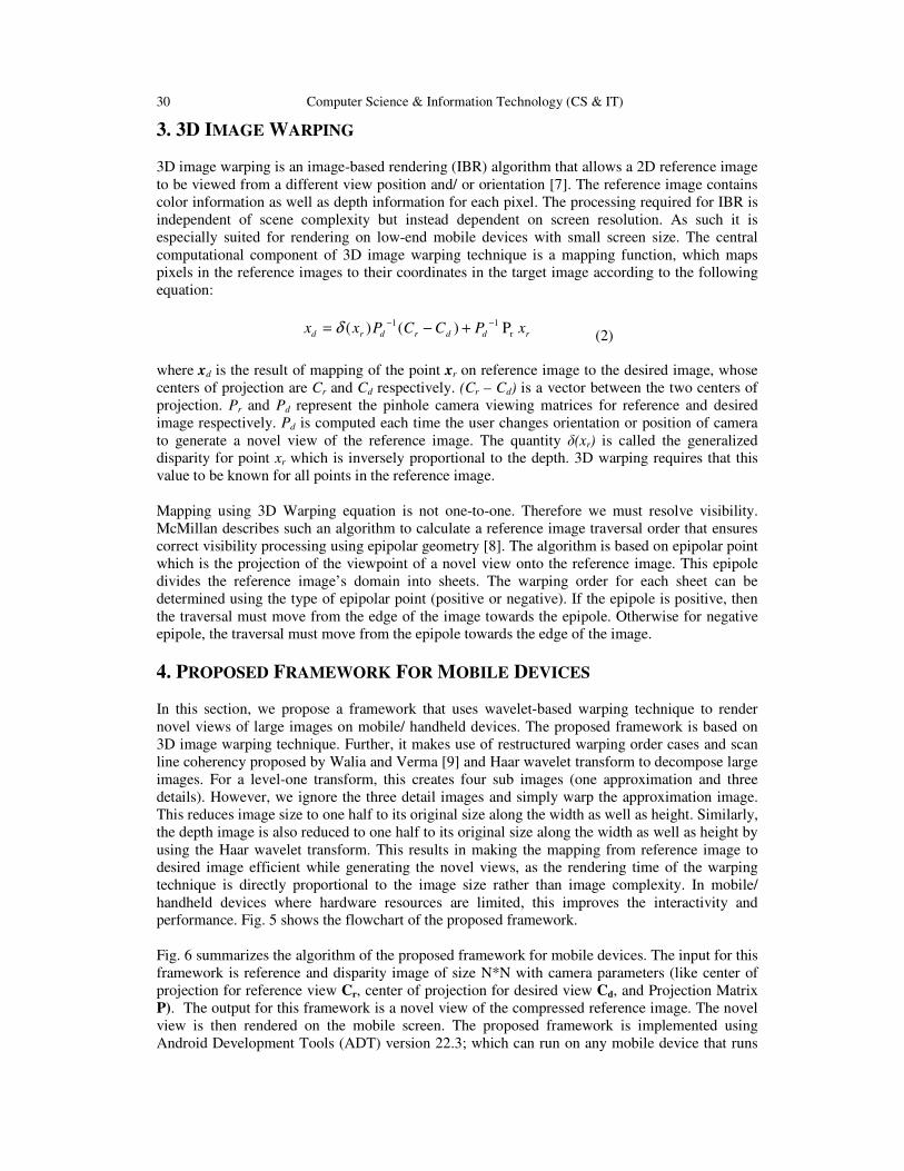
30 Computer Science & Information Technology (CS & IT)
3. 3D IMAGE WARPING
3D image warping is an image-based rendering (IBR) algorithm that allows a 2D reference image
to be viewed from a different view position and/ or orientation [7]. The reference image contains
color information as well as depth information for each pixel. The processing required for IBR is
independent of scene complexity but instead dependent on screen resolution. As such it is
especially suited for rendering on low-end mobile devices with small screen size. The central
computational component of 3D image warping technique is a mapping function, which maps
pixels in the reference images to their coordinates in the target image according to the following
equation:
1 1
r( ) ( ) Pd r d r d d rx x P C C P xδ− −
= − + (2)
where xd is the result of mapping of the point xr on reference image to the desired image, whose
centers of projection are Cr and Cd respectively. (Cr – Cd) is a vector between the two centers of
projection. Pr and Pd represent the pinhole camera viewing matrices for reference and desired
image respectively. Pd is computed each time the user changes orientation or position of camera
to generate a novel view of the reference image. The quantity δ(xr) is called the generalized
disparity for point xr which is inversely proportional to the depth. 3D warping requires that this
value to be known for all points in the reference image.
Mapping using 3D Warping equation is not one-to-one. Therefore we must resolve visibility.
McMillan describes such an algorithm to calculate a reference image traversal order that ensures
correct visibility processing using epipolar geometry [8]. The algorithm is based on epipolar point
which is the projection of the viewpoint of a novel view onto the reference image. This epipole
divides the reference image’s domain into sheets. The warping order for each sheet can be
determined using the type of epipolar point (positive or negative). If the epipole is positive, then
the traversal must move from the edge of the image towards the epipole. Otherwise for negative
epipole, the traversal must move from the epipole towards the edge of the image.
4. PROPOSED FRAMEWORK FOR MOBILE DEVICES
In this section, we propose a framework that uses wavelet-based warping technique to render
novel views of large images on mobile/ handheld devices. The proposed framework is based on
3D image warping technique. Further, it makes use of restructured warping order cases and scan
line coherency proposed by Walia and Verma [9] and Haar wavelet transform to decompose large
images. For a level-one transform, this creates four sub images (one approximation and three
details). However, we ignore the three detail images and simply warp the approximation image.
This reduces image size to one half to its original size along the width as well as height. Similarly,
the depth image is also reduced to one half to its original size along the width as well as height by
using the Haar wavelet transform. This results in making the mapping from reference image to
desired image efficient while generating the novel views, as the rendering time of the warping
technique is directly proportional to the image size rather than image complexity. In mobile/
handheld devices where hardware resources are limited, this improves the interactivity and
performance. Fig. 5 shows the flowchart of the proposed framework.
Fig. 6 summarizes the algorithm of the proposed framework for mobile devices. The input for this
framework is reference and disparity image of size N*N with camera parameters (like center of
projection for reference view Cr, center of projection for desired view Cd, and Projection Matrix
P). The output for this framework is a novel view of the compressed reference image. The novel
view is then rendered on the mobile screen. The proposed framework is implemented using
Android Development Tools (ADT) version 22.3; which can run on any mobile device that runs
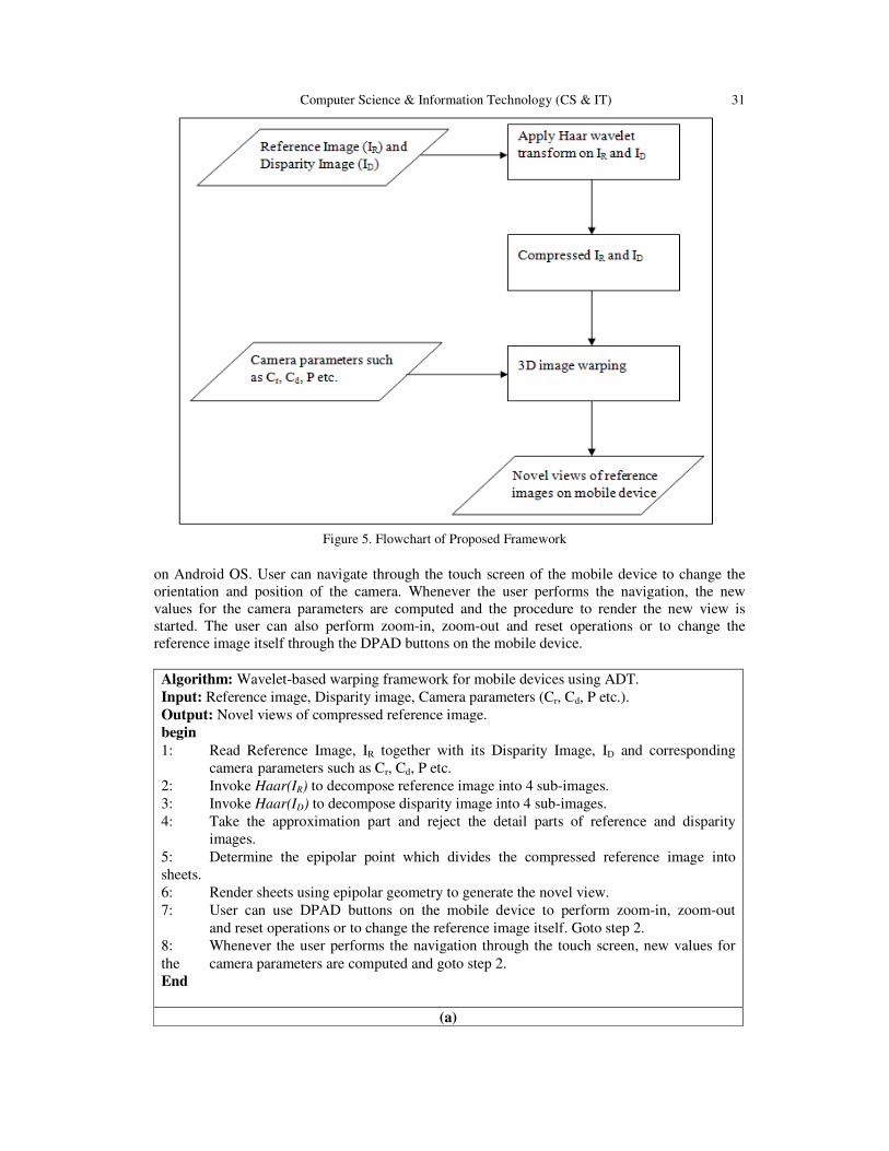
Computer Science & Information Technology (CS & IT) 31
on Android OS. User can navigate through the touch screen of the mobile device to change the
orientation and position of the camera. Whenever the user performs the navigation, the new
values for the camera parameters are computed and the procedure to render the new view is
started. The user can also perform zoom-in, zoom-out and reset operations or to change the
reference image itself through the DPAD buttons on the mobile device.
Algorithm: Wavelet-based warping framework for mobile devices using ADT.
Input: Reference image, Disparity image, Camera parameters (Cr, Cd, P etc.).
Output: Novel views of compressed reference image.
begin
1: Read Reference Image, IR together with its Disparity Image, ID and corresponding
camera parameters such as Cr, Cd, P etc.
2: Invoke Haar(IR) to decompose reference image into 4 sub-images.
3: Invoke Haar(ID) to decompose disparity image into 4 sub-images.
4: Take the approximation part and reject the detail parts of reference and disparity
images.
5: Determine the epipolar point which divides the compressed reference image into
sheets.
6: Render sheets using epipolar geometry to generate the novel view.
7: User can use DPAD buttons on the mobile device to perform zoom-in, zoom-out
and reset operations or to change the reference image itself. Goto step 2.
8: Whenever the user performs the navigation through the touch screen, new values for
the camera parameters are computed and goto step 2.
End
(a)
Figure 5. Flowchart of Proposed Framework

32 Computer Science & Information Technology (CS & IT)
Procedure: Haar(Image I)
begin
1: Separate RGB components of the image
2: Invoke HWT(R) to perform Haar Wavelet Transform on RED
image.
3: Invoke HWT(G) to perform Haar Wavelet Transform on GREEN component of the
image.
4: Invoke HWT(B) to perform Haar Wavelet Transform on BLUE component of the
image.
5: Combine RGB components of the image.
end
Procedure: HWT(Image Component Matrix
begin
1: For each row in the image matrix:
a) Find the average of each pair of values.
b) Find the difference of each pair of values.
c) Fill the first half with averages.
d) Fill the second half with differences.
e) Select the first half and repeat the process until it has one
2: For each column in the image matrix:
a) Find the average of each pair of values.
b) Find the difference of each pair of values.
c) Fill the first half with averages.
d) Fill the second half with differences.
e) Select the first half and repeat the process unt
3: This produces the updated image matrix containing approximation and detail parts.
end
Figure 6. Proposed Framework (a) Complete algorithm (b) P
5. EXPERIMENTAL RESULTS
The proposed framework has been implemented using
(update 21) and Android Development Tools (
conducted using Android Virtual Device (AVD)
Core(TM) i5 CPU and 4.0 GB RAM.
been used in our experiments. Fig. 7
(having depth information).
Image1 (512 x 512 pixels)
Figure 7
Computer Science & Information Technology (CS & IT)
Separate RGB components of the image I.
to perform Haar Wavelet Transform on RED component of the
to perform Haar Wavelet Transform on GREEN component of the
to perform Haar Wavelet Transform on BLUE component of the
Combine RGB components of the image.
(b)
Image Component Matrix)
each row in the image matrix:
Find the average of each pair of values.
Find the difference of each pair of values.
Fill the first half with averages.
Fill the second half with differences.
Select the first half and repeat the process until it has one element.
For each column in the image matrix:
Find the average of each pair of values.
Find the difference of each pair of values.
Fill the first half with averages.
Fill the second half with differences.
Select the first half and repeat the process until it has one element.
This produces the updated image matrix containing approximation and detail parts.
(c)
ramework (a) Complete algorithm (b) Procedure Haar (c) Procedure HWT
ESULTS AND DISCUSSION
The proposed framework has been implemented using Java Platform Standard Edition 1.6
(update 21) and Android Development Tools (ADT) version 22.3. The experiments have been
Android Virtual Device (AVD) emulator on a machine having 2.5 GHz Intel(R)
Core(TM) i5 CPU and 4.0 GB RAM. A set of images taken from a dataset of images
used in our experiments. Fig. 7 shows a subset of images along with their gray scale images
Image2 (512 x 512 pixels) Image3 (512 x 512
Figure 7. Images (with their depth information)
component of the
to perform Haar Wavelet Transform on GREEN component of the
to perform Haar Wavelet Transform on BLUE component of the
element.
il it has one element.
This produces the updated image matrix containing approximation and detail parts.
rocedure HWT
tandard Edition 1.6
xperiments have been
on a machine having 2.5 GHz Intel(R)
A set of images taken from a dataset of images [10] has
of images along with their gray scale images
512 pixels)

Computer Science & Information Technology (CS & IT) 33
In the setup discussed above, experiments have been conducted to evaluate the performance of
proposed framework in Android environment on a set of images shown in Fig. 7. The ADT can
be used to define AVD (Android Virtual Device) emulators that enable us to simulate the mobile
environment on a PC. Fig. 8 shows the output of the proposed rendering framework in the AVD
emulator having screen size 3.2” with 512 MB RAM.
Figure 8. Rendering using proposed framework in AVD emulator
Table 1 gives the rendering times (in milliseconds) of the different images using the proposed
framework and its comparison with the warping framework proposed by [9] using ADT. The
experimental results show that the proposed framework gives better results for compressed
images in terms of rendering time. Further as shown in Fig. 8, the compressed rebuilt image is
close to the original image.
Table 1. Rendering time comparison of images shown in Fig. 6
Images Rendering time using warping
framework [9] (in ms)
Rendering time using wavelet-
based warping framework (in ms)
Image1 3490 2278
Image2 3454 2293
Image3 3462 2232
6. CONCLUSION In this paper we propose a wavelet-based warping framework to render novel views of a reference
image on mobile devices. By applying the Haar wavelet transform we represent the reference and
disparity images in terms of low-resolution images and a set of detail coefficients. By ignoring the
detail coefficients and simply warping the approximation image we get the novel view of the
reference image. As the rendering time of the warping technique is directly proportional to the
image size rather than image complexity, this improves the rendering time. The framework is
implemented with Android Development Tools (ADT) and its performance is evaluated. The
experimental results show the proposed framework gives better results for compressed images in
terms of rendering time. Further, the compressed rebuilt image is close to the original image.
34 Computer Science & Information Technology (CS & IT)
REFERENCES
[1] M. Vetterli and J. Kovacevic, “Wavelet and Subband Coding”, Prentice Hall PTR, Englewood Cliffs,
NJ, 2007.
[2] R. S. Stankovic and B. J. Falkowski, “The Haar wavelet transform: its status and achievements”,
Computers and Electrical Engineering, Vol.29, No.1, January 2003, pp. 25-44.
[3] Eric J. Stollnitz, Tony D. DeRose and David H. Salesin, “Wavelets for Computer Graphics: A Primer
Part 1”, IEEE Computer Graphics and Applications, May 1995.
[4] N. Ahmed, T. Natarajan, and K. R. Rao, “Discrete Cosine Transform”, IEEE Trans. Computers, vol.
C-23, Jan. 1974.
[5] A. Cohen, I. Daubechies and J. C. Feauveau, "Biorthogonal bases of compactly supported wavelets",
Communications on Pure and Applied Mathematics, Vol. 45, No. 5, 1992, pp. 485–560.
[6] I. Daubechies, “Ten lectures on wavelets”, Vol. 61 of CBMS-NSF Regional Conference Series in
Applied Mathematics. Philadelphia, PA: Society for Industrial and Applied Mathematics (SIAM),
1992.
[7] L. McMillan, “An Image-Based Approach to Three-Dimensional Computer Graphics”, Ph.D. Thesis,
Department of Computer Science, University of North Carolina at Chapel Hill, 1997.
[8] L. McMillan. “Computing Visibility Without Depth”. Computer Science Technical Report TR95-047,
University of North Carolina, Chapel Hill, 1995.
[9] E. Walia and V. Verma, “A Computationally Efficient Framework for 3D Warping Technique”,
International Journal of Computer Graphics, Vol. 3, No. 1, May 2012, pp.1-10.
[10] Middlebury Stereo Datasets. http://vision.middlebury.edu/stereo/data/ scenes2006.
AUTHORS
Ekta Walia received her Bachelors degree in Computer Science from Kurukshetra
University, India and Masters in Computer Applications as well as Ph.D. (Computer
Science) from Punjabi University, Patiala, India respectively. After starting her
professional career as a software consultant with DCM DataSystems, New Delhi, India,
in 1998, she served as faculty member in the National Institute of Technical Teachers
Training and Research (NITTTR), Chandigarh, India for 07 years. From 2007 to 2011,
she served in various academic institutes. In July 2011, she joined the Department of
Computer Science in South Asian University, New Delhi, where she has been serving as
Associate Professor & Chairperson. Her research interests include 3D Rendering, Digital Image
Watermarking, Content Based Image Retrieval and Face Recognition. She has a number of international
journal and conference publications in these areas. She has been on the reviewing board of many reputed
image processing journals and conferences. She has also chaired sessions in International Conferences of
repute.
Vishal Verma is an Assistant Professor at Department of Computer Science, M. L. N.
College, Yamuna Nagar, Haryana (INDIA). He is having Masters in Computer
Applications from Kurukshetra University, Kurukshetra (INDIA) and M. Phil. (Computer
Science) from Madurai Kamaraj University, Madurai (INDIA). His total teaching
experience is more than 12 years and is presently pursuing Ph.D. (Computer Science) at
Maharishi Markandeshwar University, Mullana, Ambala (INDIA). His current research
focus is on Rendering Techniques and Image Processing. He has a number of
International journal and conference papers to his credit.
Natarajan Meghanathan et al. (Eds) : ICAIT, ICDIPV, ITCSE, NC - 2014
pp. 35–41, 2014. © CS & IT-CSCP 2014 DOI : 10.5121/csit.2014.4705
ADAPTIVE TRILATERAL FILTER
FOR IN-LOOP FILTERING
Akitha Kesireddy and Mohamed El-Sharkawy
Purdue School of Engineering and Technology
ABSTRACT
High Efficiency Video Coding (HEVC) has achieved significant coding efficiency improvement
beyond existing video coding standard by employing several new coding tools. Deblocking
Filter, Sample Adaptive Offset (SAO) and Adaptive Loop Filter (ALF) for in-loop filtering are
currently introduced for the HEVC standard. However, these filters are implemented in spatial
domain despite the fact of temporal correlation within video sequences. To reduce the artifacts
and better align object boundaries in video, a proposed algorithm in in-loop filtering is
proposed. The proposed algorithm is implemented in HM-11.0 software. This proposed
algorithm allows an average bitrate reduction of about 0.7% and improves the PSNR of the
decoded frame by 0.05%, 0.30% and 0.35% in luminance and chroma.
KEYWORDS
HEVC, Trilateral Filter and In-Loop Filter.
1. INTRODUCTION
HEVC is the new video coding standard developed by the joint collaboration of the ITU-T Video
Coding Experts Group (VCEG) and the ISO/IEC Moving Picture Experts Group (MPEG). The
main aim of the HEVC is improving the compression efficiency of the H.264/AVC standard by
almost 50% and maintaining the same computational complexity. Many coding tools are included
to reduce the distortion between the original frames and decoded frames produced by the lossy
coding.
The name loop filtering reflects that the filtering is done by removing the blocking artifacts
[1].H.264/AVC includes an in-loop Deblocking filter. HEVC employs a Deblocking filter similar
to the one used in H.264/AVC but expands an in-loop processing by introducing two new tools:
SAO and ALF. These techniques are implemented to reduce the distortion introduced by the
encoding process(prediction, transform, and quantization). By including these filtering
techniques, the pictures will serve as better references for motion- compensated prediction since
they have less encoding distortion.
Over the past several years many algorithms have been proposed for reducing the blocking
artifacts and the bit rate [2] – [5]. These algorithms can be categories into three types: first type is
a post processing algorithm for removing blocking artifacts for highly compressed images in the
DCT domain [2], second one reduces the blocking artifacts carried out at encoding schemes and
third one reduces the temporal redundancy of ALF parameters by reusing the prior transmitted
filter parameters [3]. In [4],a strong filter is selectively applied to blocks having small artifacts to

36 Computer Science & Information Technology (CS & IT)
avoid harmful side effect of filtering. A weak filter is applied to the other blocks to slightly
correct them. In [5],an adaptive in-loop bilateral filter selecting the optimal filter parameters,
based on the image characteristics, is proposed to minimise the Lagrangian Rate-Distortion.
In this paper, we propose an algorithm to reduce the bit rate and improve the video quality by
combining a trilateral filter and adaptive filter together, evaluate the effect of proposed algorithm
on the quality of the output and compare their results to the evaluated results of the original
algorithm of HEVC for various quantization parameters.
The rest of the paperis organized as follows: Section II describes the adaptive loop filtering.
Section III describes the trilateral filter. Section IV describes the proposed algorithm. Finally, the
experimental results and conclusion are shown in sections V and VI.
2. HEVC ADAPTIVE LOOP FILTERING
This section describes ALF core techniques employed in the final ALF version in HM-11.0. The
filter includes Wiener filter, filter shapes, and coefficient coding. The Wiener filter minimizes the
mean square error between the desired samples and the filtered samples. The desired samples are
the original picture. The to-be-filtered samples are the output picture of SAO. The filtered
samples are the output picture of ALF.
In [1], an ALF is applied to the reconstructed signal after the de-blocking filter and SAO. The
filter is adaptive in the sense that the coefficients are signalled in the bit stream and can therefore
be designed based on image content and distortion of the reconstructed picture. The filter is used
to restore the reconstructed picture such that the mean-squared error between the source picture
and the reconstructed picture is minimized.
Test Model HM-3.0 uses a single filter shape which is a cross overlaid on a 3 x 3 square with nine
coefficients, to be encoded in the bit stream. The number of taps in the filter is greater than nine
due to symmetry; however, every picture may not need all the nine taps as in HM-7.0 [6]. This
test model has different filter square shapes 5X5, 7X7 and 9X9, where these shapes can be
selected for different pictures. In HM-6.0 and HM-7.0, number of coefficients is reduced to half
by changing the ALF from square to diamond shape. The combination of 9X7-tap cross shape
and 3X3-tap rectangular shape generates the filter shape of ALF in HM-7.0.The Filter coefficients
are derived by solving Wiener-Hopf equation [6].ALF in HM7.0 reduces the number of
coefficient by half which in turn reduces the number of multiplications by half, which
significantly reduces the chip area for ALF.
Figure 1: Filter shape of ALF in HM-6.0 and HM-7.0.

Computer Science & Information Technology (CS & IT) 37
Figure 2: Locations of ALF parameters in the bit stream.
Syntax Design
There are two types of coded information for ALF: filter coefficient parameters and filter on/off
control flags. As shown in Fig. 2, the filter coefficient parameters are located in a picture-level
header called APS, and the filter on/off control flags are interleaved in slice data with CTUs. The
filter coefficient parameters include picture-level on/off control flags for three color components,
number of luma filters (i.e., class/region merging syntax elements for BA/RA), and corresponding
filter coefficients. Up to 16 luma filters, one Cb filter, and one Cr filter per picture can be
signalled. Filter on/off control flags are used to provide better local adaptation. In addition to the
picture-level filter on/off control flags in APS, there are also slice-level and CTU-level filter
on/off control flags. In slice header, similarly, filter on/off control flags for three color
components are coded. The signalling of slice-level filter on/off control flags can solve a slice
parsing problem when the referenced APS of the slice is lost [7]. If the slice-level on/off control
flag indicates ALF-on, CTU-level filter on/off control flags are interleaved in slice data and coded
with CTUs; otherwise, no additional CTU-level filter on/off control flags are coded and all CTUs
of the slice are inferred as ALF-off.
APS was removed from HEVC standard after HM-8.0.
As APS is removed the related syntax elements of filter parameters in slice header ALF is
implemented.
Trilateral Filter
An image is defined by f(x) ∈ (n = dimensionality), where x ∈ Ω is the pixel position in
image domain Ω. Generally speaking, an n-D (n-dimensional) pixel-discrete image has an image
domain defined as,∅ ⊂ Ω ⊆ ⊂ (Xn is our maximum discrete index set of the image domain
in dimension n). A smoothing operator will reduce an image to a smoothed version of itself,
specifically S(f) = s, where s is in the same image domain as f. To introduce the trilateral filter, we
must first define the bilateral [8] case; we will then go on to define the traditional trilateral filter
using this notation.
The trilateral filter is a “gradient-preserving” filter [8]. It aims at applying a bilateral filter on the
current plane of the image signal. The trilateral case only requires the specification of one
parameter . At first, a bilateral filter is applied on the derivatives of (i.e., the gradients):
= 1∇ ∇ + ⋅ ⋅ ‖∇ + − ∇ ‖Ω
∇ = ⋅ ‖∇ + − ∇ ‖Ω
To approximate∇ , forward differences are used, and more advanced techniques (e.g., Sobel
gradients, 5-point stencil) are left for future studies. For the subsequent second bilateral filter,
suggested the use of the smoothed gradient [instead of ∇ for estimating an
approximating plane

38 Computer Science & Information Technology (CS & IT)
, = + ⋅
Let ∇, = + − , . Furthermore, a neighbour-hood function
+ = "1 # $ + − $ < &0 ()ℎ+,#-+. is used for the second weighting. Parameter c specifies the adaptive region and is discussed
further below. Finally,
- = + 1∇ ∇ , ⋅ ⋅ ∇ , ⋅ N, Ω
∇ = ⋅ ∇ , ⋅ N, Ω
The smoothed function s equals 012 .
Again, and are assumed to be Gaussian functions, with standard deviations
and, respectively. The method requires specification of parameter only, which is at first used
to be the diameter of circular neighbour-hoods at x in ; let 333be the mean gradient of in
such a neighbourhood. The parameter for is defined as follows: = 4 ∙ 6max:∈Ω 333 − min:∈Ω 3336 (4 =0:15 was chosen). Finally,& = .
3. PROPOSED ALGORITHM
There are three in-loop filtering techniques in HEVC; namely, the de-blocking filtering, the
Sample Adaptive Offset (SAO) and the Adaptive Loop Filter (ALF). After the details of these
filters in the previous sections, we design the proposed filter in in-loop filtering process.
Boundary Block Detection Trilateral filter works in the context of block-based processing. The trilateral filter might
introduce other blocking artifacts if it is applied to all the blocks in a frame, so it is only applied
to blocks in object boundaries. This is called region-based filtering. The standard deviation of the
block is used to detect where the boundary block. Non-boundary blocks usually consist of
homogeneous pixel values and have a smaller variance. When the standard deviation of a block
exceeds a pre-defined value, the trilateral filtering is performed and the standard deviation for an
NXN block is:
STD = Sqrt C 1N × N E E.FIi, j − MeanKLM].OPQRST
PQUST
. Where N is the block size, I(i,j) is the pixel intensity, and Mean is the mean of the block.
In-Loop Filtering
After the details of ALF and trilateral filter in SECTION II, it is now essential to define how to
combine these filters in the HEVC in-loop filtering process. As described in the introduction. The
trilateral filter is “gradient-preserving” filter suited to remove the blocking artifacts whereas the
Adaptive loop filter is more targeted to reduce the bit-rate. Therefore, it is appropriate to combine
these two filters by selecting, for each image block in the reconstructed frame. This is the main
idea behind the proposed algorithm whose processing considered each block along with the de-
blocking filter. The filtering reduces the bit-rate and improves the PSNR values and is not

Computer Science & Information Technology (CS & IT) 39
complicated when compared with other algorithms. Now the procedure is detailed in steps by
supposing a input frame F into the in-loop filter. The performed steps are:
1. Partition F into block size of B
2. Using the standard deviation of a block detect the object boundaries
3. Over the object boundary perform TLF to obtain FWXY
4. Perform DBF over the remaining blocks of the frame to obtain FZ[Y
5. Finally the combined frame FWZ[Y is obtained
6. Over the whole frame FWZ[Y perform ALF to obtainFWZ\XY.
In this algorithm by considering the region characteristics of the block only the block boundaries
are filtered by trilateral filter. Therefore, we adopt the quad-tree structure of LCU in HEVC. For
every CUs in LCU, we check whether its standard deviation is above a certain threshold. If the
condition is met, we perform the trilateral filtering in this block. Later ALF is performed over the
whole frame. The overall flow chart of the proposed in-loop filter for HEVC is shown in Figure 3
Figure 3: Flow chart of the proposed algorithm.
4. EXPERIMENTAL RESULTS
In this paper, the proposed method is implemented on HM-11.0 and the results are obtained for
both the modified HM11.0 and the original one. For each video sequence, the quantization
parameters are 32, 38 and 42. Five frames in the test sequence are encoded. Figures 4 and 5 show
the PSNR for different bit rates. Figure 6 compares the subjective video quality (better quality
can be shown on a screen).

40 Computer Science & Information Technology (CS & IT)
Figure 6: (a) input picture (b) reconstructed picture using (c) reconstructed picture using
original software proposed software
Figure 4:PSNR for different bit rates using Foreman.
Figure 5: PSNR for different bit rates using Flower.

Computer Science & Information Technology (CS & IT) 41
Table 1: Flower YUV.
QP Bitrate
changes %
Y-
PSNR
U-
PSNR
V-
PSNR
32 0.69 0.03 0.10 0.18
38 0.66 0.05 0.21 0.27
42 0.65 0.07 0.34 0.35
Table 1: Bit-rate and PSNR changes for test sequence
Table 2:Bit-rate and PSNR changes for test sequence
Tables 1 and 2 show that the proposed algorithm reduces the bit rate by 0.7% and improves the
PSNR values by 0.05%, 0.30 % and 0.35 %in luminance and chroma. Improvement is more
significant on low resolution than the high resolution video sequences.
5. CONCLUSION
In this paper, the main aim of proposing a new adaptive trilateral filter for in-loop filtering is to
reduce the bit-rate and improve the PSNR values. The simulation results show that the proposed
algorithm improves rate distortion performance and reduces the ringing artifacts introduced by the
use of large transform block sizes and, therefore, it also improves the perceived video quality.
Moreover, proposed algorithm allows an average bitrate reduction of about 0.7% and improves
the PSNR of the decoded frame by 0.05%, 0.30% and 0.35% in luminance and chroma.
REFERENCES
[1]. M. T. Pourazad, C. Doutre, M. Azimi, and P. Nasiopoulos“ HEVC: The New Gold Standard for Video
Compression,” IEEE consumer electronics magazine, July 2012.
[2]. R. Palaparthi, V. K. Srivastava “A Simple Deblocking Method for Reduction of Blocking Artifacts,”
IEEE Students’ Conference on Electrical, Electronics and Computer Science,2012.
[3]. X. Zhang, C. R. Xiong and S. Ma, “Adaptive Loop Filter with Temporal Prediction,” 2012 Picture
Coding Symposium, May 7 - 9, 2012, Kraków, Poland.
[4]. K. Q. Dinh and H. Shim“DEBLOCKING FILTER FOR ARTIFACT REDUCTION IN
DISTRIBUTED COMPRESSIVE VIDEO SENSING”VCIP,page 1-5 ,IEEE(2012)
[5]. M. Naccari and F. Pereira, Instituto de Telecomunicações “Adaptive Bilateral Filter for Improved In-
Loop Filtering in the Emerging High Efficiency Video Coding Standard,” 2012 Picture Coding
Symposium May 7-9, 2012, Kraków, Poland.
[6]. C. Y. Tsai, Member, IEEE, C. Y. Chen, T. Yamakage“Adaptive loop filter for video coding.”IEEE
Journal of selected topics in signal processing Vol.7 N0. 6 ,December 2013.
[7]. S. Esenlik, M. Narroschke, and T.Wedi, “Syntax refinements for SAO and ALF,” , Joint Collaborative
Team on Video Coding (JCT-VC) of ISO/IEC MPEG and ITU-T VCEG, JCTVC-G566, Nov. 2011..
[8]. http://www.researchgate.net/publication/37988010_Fast_Trilateral_Filtering/file/d912f50d172f2
a9ecf.pdf
[9]. http://www.apsipa.org/proceedings_2012/papers/102.pdf.
Table 2: Foreman YUV.
QP Bitrate
changes %
Y-
PSNR
U-
PSNR
V-PSNR
32 0.67 0.05 0.245 0.291
38 0.65 0.039 0.338 0.349
42 0.63 0.035 0.157 0.156

42 Computer Science & Information Technology (CS & IT)
INTENTIONAL BLANK

Natarajan Meghanathan et al. (Eds) : ICAIT, ICDIPV, ITCSE, NC - 2014
pp. 43–54, 2014. © CS & IT-CSCP 2014 DOI : 10.5121/csit.2014.4706
A CLOUD SERVICE SELECTION MODEL BASED
ON USER-SPECIFIED QUALITY OF SERVICE
LEVEL
Chang-Ling Hsu
Department of Information Management, Ming Chuan University,
Taoyuan, Taiwan [email protected]
ABSTRACT Recently, it emerges lots of cloud services in the cloud service market. After many candidate
services are initially chosen by satisfying both the behavior and functional criteria of a target
cloud service. Service consumers need a selection model to further evaluate nonfunctional QOS
properties of the candidate services. Some prior works have focused on objective and
quantitative benchmark-testing of QOS by some tools or trusted third-party brokers, as well as
reputation from customers. Service levels have been offered and designated by cloud service
providers in their Service Level Agreement (SLA). Conversely, in order to meet user
requirement, it is important for users to discover their own optimal parameter portfolio for
service level. However, some prior works focus only on specific kinds of cloud services, or
require users to involve in some evaluating process. In general, the prior works cannot evaluate
the nonfunctional properties and select the optimal service which satisfies both user-specified
service level and goals most either. Therefore, the aim of this study is to propose a cloud service
selection model, CloudEval, to evaluate the nonfunctional properties and select the optimal
service which satisfies both user-specified service level and goals most. CloudEval applies a
well-known multi-attribute decision making technique, Grey Relational Analysis, to the
selection process. Finally, we conduct some experiments. The experimental results show that
CloudEval is effective, especially while the quantity of the candidate cloud services is much
larger than human raters can handle.
KEYWORDS Cloud Service, Cloud Service Selection, Multi-attribute Decision Model, Quality of Service,
Cloud Computing
1. INTRODUCTION
Emerging cloud computing and its application emphasize on lower Total Cost of Ownership
(TCO), that pay as you go for the cloud services. It makes a user through the application of cloud
services to reduce TCO and energy consumption. A cloud interactive model over Internet is
composed of two parts: a cloud client and a cloud service. Common applications of a cloud client
are such as web pages and mobile applications. As for categories of cloud services, NIST has
defined three cloud service models: Software as a Service (SaaS), Platform as a Service (PaaS)
and Infrastructure as a Service (IaaS) [1].
44 Computer Science & Information Technology (CS & IT)
Recently, it emerges lots of cloud services in the cloud service market. Enterprises need to select
suitable cloud services effectively to meet the requirements of an enterprise information systems
and their integration. If a suitable cloud service could be integrated into an enterprise information
system, the quality of the information system would be better than one with an un-suitable cloud
service. Khezrian et al. [2] deem that two significant tasks in the process of a selection model are
selection and ranking in which every solution for them is affected directly on description of
services. During describing a service, three properties have to be considered: behavior, functional,
and nonfunctional. The candidate services are initially chosen by satisfying both the behavior and
functional criteria of a target cloud service. As there are often many cloud services that meet the
functional and behavior requirements, the cloud service selection uses some criteria to select the
optimal service. However, in real world practice, there are too large a number of possible
candidate cloud services to select manually. Thus, service consumers need a selection model to
further evaluate nonfunctional properties of the candidate services, such as Quality of Service
(QOS), price and reputation.
Besides, service levels have been offered and designated by many cloud service providers in their
Service Level Agreement (SLA). Conversely, in order to meet user requirement, it is important
for users to discover their own optimal parameter portfolio for service level. It also depends on
selection criteria of cloud services. And, the criteria of cloud service have dynamic, invisible,
variant, subjective and vague characteristics. Therefore, it is a multi-attribute decision-making
problem about discovering the optimal parameter portfolio. Still, cloud providers and third-party
brokers have not had the selection and recommendation mechanisms. The criteria in previous
researches focus on benchmarks by a trusted third-party broker, such as CloudHarmony [3], based
on objective and quantitative testing of QOS, as well as reputation from customers. The criteria in
previous researches focus on benchmarks by some tools (i.e. CloudCmp [4] and vCenter Hyperic
[5]), or third-party brokers (i.e. CloudHarmony) based on objective and quantitative testing of
QOS, as well as reputation from customers.
However, some prior works [6, 7] focus only on specific kinds of cloud services, or require users
to involve in some evaluating process [7, 8]. In general, the prior works cannot evaluate the
nonfunctional properties and select the optimal service which satisfies both user-specified service
level and goals most either. Therefore, based on user-specified QOS requirement for service level,
and the objective and quantitative benchmarks, the aim of this study is to propose a new cloud
service selection model, CloudEval (Cloud Evaluator), to evaluate the nonfunctional properties
and select the optimal service which satisfies both user-specified service level and goals most.
CloudEval applies a well-known multi-attribute decision making technique, i.e. Grey Relational
Analysis, to the selection process.
The remainder of this paper is organized as follows. Section 2 reviews the related research work.
Section 3 describes CloudEval. Section 4 presents the experiments and an analysis of the results.
Finally, Section 5 draws conclusions.
2. RELATED WORK
2.1. Selection Models
In view of the limits of the prior works that we have mentioned above, now we explained about
why they cannot evaluate the nonfunctional properties and select the optimal service which
satisfies both user-specified service level and goals most. First, some prior works [6, 7] focus only
on specific kinds of cloud services (such as SaaS, web server service, or cloud storage service)
neglect wider scope benchmarks from the broker, and financial or service credit in SLA from
providers need to be further quantified and integrated during the selection. Secondly, some prior
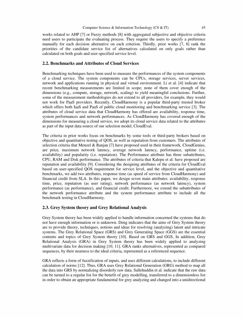
Computer Science & Information Technology (CS & IT) 45
works related to AHP [7] or Fuzzy methods [8] with aggregated subjective and objective criteria
need users to participate the evaluating process. They require the users to specify a preference
manually for each decision alternative on each criterion. Thirdly, prior works [7, 8] rank the
priorities of the candidate service list of alternatives calculated on only goals rather than
calculated on both goals and user-specified service level.
2.2. Benchmarks and Attributes of Cloud Services
Benchmarking techniques have been used to measure the performances of the system components
of a cloud service. The system components can be CPUs, storage services, server services,
network and applications running in physical and virtual environment. Li et al. [4] indicate that
recent benchmarking measurements are limited in scope; none of them cover enough of the
dimensions (e.g., compute, storage, network, scaling) to yield meaningful conclusions. Further,
some of the measurement methodologies do not extend to all providers, for example, they would
not work for PaaS providers. Recently, CloudHarmony is a popular third-party trusted broker
which offers both IaaS and PaaS of public cloud monitoring and benchmarking service [3]. The
attributes of cloud service data that CloudHarmony has offered are availability, response time,
system performances and network performances. As CloudHarmony has covered enough of the
dimensions for measuring a cloud service, we adopt its cloud service data related to the attributes
as part of the input data source of our selection model, CloudEval.
The criteria in prior works focus on benchmarks by some tools or third-party brokers based on
objective and quantitative testing of QOS, as well as reputation from customers. The attributes of
selection criteria that Menzel & Ranjan [7] have proposed used in their framework, CloudGenius,
are price, maximum network latency, average network latency, performance, uptime (i.e.
availability) and popularity (i.e. reputation). The Performance attribute has three subattributes,
CPU, RAM and Disk performance. The attributes of criteria that Kalepu et al. have proposed are
reputation and availability [9]. Considering the designing attributes of the criteria for CloudEval
based on user-specified QOS requirement for service level, and the objective and quantitative
benchmarks, we add two attributes, response time (as speed of service from CloudHarmony) and
financial credit from SLA. In this paper, we design seven main attributes: availability, response
time, price, reputation (as user rating), network performance (as network latency), system
performance (as performance), and financial credit. Furthermore, we extend the subattributes of
the network performance attribute and the system performance attribute to include all the
benchmark testing in CloudHarmony.
2.3. Grey System theory and Grey Relational Analysis
Grey System theory has been widely applied to handle information concerned the systems that do
not have enough information or is unknown. Deng indicates that the aims of Grey System theory
are to provide theory, techniques, notions and ideas for resolving (analyzing) latent and intricate
systems. The Grey Relational Space (GRS) and Grey Generating Space (GGS) are the essential
contents and topics of Grey System theory [10]. Based on GRS and GGS, In addition, Grey
Relational Analysis (GRA) in Grey System theory has been widely applied to analyzing
multivariate data for decision making [10, 11]. GRA ranks alternatives, represented as compared
sequences, by their nearness to the ideal criteria, represented as a referenced sequence.
GRA reflects a form of fuzzification of inputs, and uses different calculations, to include different
calculation of norms [12]. Thus, GRA uses Grey Relational Generation (GRG) method to map all
the data into GRS by normalizing disorderly raw data. Sallehuddin et al. indicate that the raw data
can be turned to a regular list for the benefit of grey modelling, transferred to a dimensionless list
in order to obtain an appropriate fundamental for grey analyzing and changed into a unidirectional

46 Computer Science & Information Technology (CS & IT)
series for decision making [11]. GRA calculates a Grey Relational Coefficient (GRC) for each
dimension (i.e. attribute), and then it calculates a grey relational grade by averaging all GRCs of
each dimension for each compared sequence of the dimensionless list. Above all, GRA is simple,
practical, and demands less precise information than other methods. Therefore, we adopt GRA
method to select the optimal service which satisfies user-specified service level most.
3. THE CLOUD SERVICE SELECTION MODEL
The stakeholders of CloudEval are users, third-party brokers of cloud service and cloud service
providers. The design of data sources for CloudEval is SLAs from providers and any trusted
third-party brokers, such as CloudHarmony, which offers reputation of providers, some objective
and quantitative benchmark-testing data. CloudEval consists of two components: selection
process and data structure. We describe both components respectively as follows.
3.1. Selection Process
We apply the well-known multi-attribute decision making technique, Grey Relational Analysis, to
our selection process. The service selection process is as follows.
1st step. Setting user selection criteria, goals and their weights: a user sets one’s selection criteria
of cloud service, acting as a referenced sequence in GRA, and sets weight and goal for each
attribute. The goals are represented with preference for value of an attribute of the selection
criteria.
2nd step. Normalizing the candidate list: we normalize each cloud service acting as a compared
sequence of the candidate list in GRG method.
3rd step. Calculating Grey Relational Coefficient (GRC) of the attributes of each service: we use
Deng’s method [13] to calculate all GRCs of the attributes of each cloud service based on the
comparison between each compared sequence and the referenced sequence.
4th step. Calculating grey relational grade for each service: we calculate a grey relational grade
for each cloud service by averaging all the grey relational coefficient of each attribute. As for the
way of averaging all the grey relational coefficient, we use both Deng’s equal-weighted average
method [13] and weighted average method.
5th step. Ranking the list: we rank the candidate list by ordering grey relational grade of each
service. Finally, we choose the largest grey relational grade in the ranked list as the optimal
service which satisfies user-specified service level most.
3.2. Data structure
Each cloud service of provider j is a compared sequence, X[j] = (x1, x2, …, xm) ∈ Domain(A1)
×…× Domain(Ai) × …× Domain(Am), where j = 1..n. X[0] is a referenced sequence in GRA.
Both X[0] and X[j] have a fixed-length vector with attribute-value pairs of a data instance, Ai is
an attribute of X, i =1..m. As mentioned in Section 2.2, we have designed the seven main
attributes of selection criteria. The attributes availability, response time, network performance,
system performance and financial credit are QOS-related and the attribute user rating and price
are not QOS-related. As for the goals for each attribute of the selection criteria, the bigger the
better are the attributes availability, user rating, network performance, system performance and
financial credit; the less the better are the attributes response time and price. We design the
attributes in detail as follows.

Computer Science & Information Technology (CS & IT) 47
3.2.1. Availability
It is also known as the uptime status, the percentage of available connectivity time during a time
period from a service provider. When a remote cloud service is usable as a user connects the
service online, we call the time connectivity time; When a remote cloud service is unusable, it
might be offline, under maintenance, shutdown, breakdown or instable as a user connects the
service online. We call the time connectivity downtime. We define availability as:
availability = (1)
3.2.2. Response Time
It is also called as round trip time or speed to represent the time duration between sending out a
request and receiving a response to a service user. Its measured unit maybe second or millisecond.
3.2.3. User Rating
Some customers have rated each cloud service according to their usage experiences of the service
on some broker websites. It is often rated from 0 to 5. A user refers to the rating as a social
reputation.
3.2.4. Price
Due to budget limit, a user will consider the announced pricing published by a provider. The
pricing is on a per-use basis, which maybe per minute, hour, day, or month, under different
system environment configurations of instance type of a cloud service. The environment
configurations could contains number of CPU cores, size of RAM and storage, network
throughput, etc.
3.2.5. Network Performance
Suppose each benchmark item of network performance of a cloud service collected from a broker,
n[i, j], where i is the i-th benchmark item, and j is the j-th provider. The measured unit of each
benchmark item is MBS (Mega-Bits per Second) for throughput. Due to metric of each
benchmark item has different value range, we set the scale of the network performance from 0 to
1. Thus, we normalize each benchmark item as:
net[i, j] = (2)
where max_thput[i]: the maximum average summary network performance among all the i-th
benchmark items of each provider, min_thput[i]: the minimum average summary network
performance among all the i-th benchmark items of each provider. Then, we calculate the average
summary network performance for the j-th provider by weighted average scoring as:
avg_net_scores[j] = (3)
where w[i]: the user-specified weight of the i-th benchmark item.
3.2.6. System Performance
Suppose each benchmark item of system performance of a cloud service for a provider from a
broker, s[i, j], where i is the i-th benchmark item and j is the j-th provider. Due to metric of each

48 Computer Science & Information Technology (CS & IT)
benchmark item has different measured unit and value range, for instance, it is IOPS
(Input/Output Operations Per Second) for disk IO; there are ECUs (EC2 Compute Unit) [3] or
CCUs (CloudHarmony Compute Unit) [3] for CPU performances. We set the scale of all the
system performances from 0 to 1. Thus, we normalize each benchmark item as:
sys[i, j] = (4)
where max_val[i]: the maximum average summary system performance in all the i-th benchmark
items of each provider, min_val[i]: the minimum average summary system performance in all the
i-th benchmark item of each provider.
Then, we calculate the average summary system performance for the j-th provider by weighted
average scoring as:
avg_sys_scores[j] = (5)
where w[i]: the user-specified weight of the i-th benchmark item.
3.2.7. Financial Credit
It means that percentage of monthly bill (i.e. credit rate) for covered a cloud service or service
credit which does not meet the availability level in SLA from a provider that will be credited to
future monthly bills of customer [14, 15]. Each credit rate is counted on an availability interval.
As each interval of provider may be different from a similar user-specified interval, for example,
the availability intervals, [99.00%, 99.95%) vs. [98.00%, 99.96%) are shown in Table 2(a) and
Table 1 respectively. For comparability of both the credit rates in different availability intervals,
we design an algorithm, adjust-interval-credit as shown in Figure 1, to adjust each pair of the
original credit of a provider: ([99.00%, 99.95%), 10%) as shown in Table 2(a) into pair of the
adjusted credit: ([98.00%, 99.96%), 17.65%) as shown in Table 2(b).
In the algorithm, suppose each interval of financial credit or service credit of a cloud service in
SLA from a provider, cred[k, j], where k is the k-th availability interval and j is the j-th provider.
The measured unit of each interval is credit rate for a user-specified interval of monthly
availability percentage. The scale of the credit is from 0 to 1. The descriptions of some important
symbols of cred[k, j] are specified as: (1) length: the length of an interval; (2) upperBound: the
upper bound of an interval; (3) lowerBound: the lower bound of an interval; (4)
newUpperBound: the adjusted upper bound of an interval; (5) newlowerBound: the adjusted
lower bound of an interval; (6) upperBound.∆: a new interval between upperBound and
newUpperBound; (7) lowerBound.∆: a new interval between lowerBound and newLowerBound;
(8) upperBound.∆.rate: the rate of upperBound.∆; (9) upperBound.∆.length: the length of
upperBound.∆; (10) newLength: the new length of an adjusted interval; (11) middle.length: the
adjusted interval between lowerBound.∆ and upperBound.∆.
Table 1. A user-specified financial credit list.
Interval No. Availability Interval
(Monthly) Credit Rate
1 [98.00%, 99.96%) 10%
2 [94.00%, 98.00%) 25%
3 [0, 94.00%) 50%

Computer Science & Information Technology (CS & IT) 49
Table 2. The adjusted credit based on the original credit.
Original Credit List
(a) Adjusted Credit List
(b)
Interval No.
Availability Interval
Credit Rate
Availability Interval
Credit Rate
1 [99.00%,
99.95%) 10%
[98.00%,
99.96%) 17.65%
2 [95.00%,
99.00%) 25%
[94.00%,
98.00%) 31.25%
3 [0, 95.00%) 50% [0, 94.00%) 50.00%
Algorithm adjust-interval-credit(j, n, user-credit-list, provider-credit-list)
Input: j: the j-th provider; n: the number of user-specified availability intervals; user-credit-list: a list of each
user-specified pair, (interval k, credit rate c); provider-credit-list: a list of each pair of a service, (interval k,
credit rate c).
Output: an adjusted list of pair of a service, (interval k, credit rate c).
(1) initialize all the required variables;
(2) cred[1, j].length = cred[1, j].upperBound - cred[1, j].lowerBound;
(3) For each interval of provider-credit-list and user-credit-list, k = 1 to n do loop
(4) cred[k+1, j].length = cred[k+1, j].upperBound - cred[k+1, j].lowerBound;
(5) cred[k, j].newUpperBound = user[k].upperBound;
(6) If (cred[k, j].upperBound < user[k].upperBound) Then
cred[k,j].upperBound.∆.rate = cred[k, j].rate;
cred[k, j].upperBound.∆.length = user[k].upperBound - cred[k, j].upperBound;
cred[k, j].newLength = cred[k, j].length + cred[k, j].upperBound.∆.length;
(7) cred[k, j].newLowerBound = user[k].lowerBound;
(8) If (cred[k, j].lowerBound > user[k].lowerBound) Then
cred[k, j].lowerBound.∆.rate = cred[k+1, j].rate;
cred[k, j].lowerBound.∆.length = cred[k, j].lowerBound - user[k].lowerBound;
cred[k, j].newLength = cred[k, j].newLength + cred[k, j].lowerBound.∆.length;
(9) If (cred[k, j].upperBound.∆.length < 0 and cred[k, j].lowerBound.∆.length ≧ 0) Then
cred[k, j].middle.length = cred[k, j].length + cred[k, j].upperBound.∆.length;
cred[k, j].newRate = (cred[k, j].middle.length / cred[k, j].newLength) * cred[k, j].rate +
(cred[k, j].lowerBound.∆.length / cred[k, j].newLength) * cred[k, j].lowerBound.∆.rate;
(10) If (cred[k, j].upperBound.∆.length < 0 and cred[k,j].lowerBound.rate.∆.length < 0) Then
cred[k, j].middle.length = cred[k, j].length + cred[k, j].upperBound.rate.∆.length +
cred[k,j].lowerBound.rate.∆.length;
cred[k, j].newRate = cred[k, j].rate;
(11) If (cred[k, j].upperBound.∆.length ≧≧≧≧ 0 and cred[k, j].lowerBound.rate.∆.length < 0) Then
cred[k, j].middle.length = cred[k, j].length + cred[k, j].lowerBound.rate.∆.length;
cred[k, j].newRate = (cred[k, j].upperBound.∆.length / cred[k, j].newLength) *
cred[k, j].upperBound.∆.rate + (cred[k, j]. middle.length /cred[k, j].newLength) * cred[k, j].rate;
(12) If (cred[k, j].upperBound.∆.length ≧≧≧≧ 0 and cred[k, j].lowerBound.rate.∆.length ≧≧≧≧ 0) Then
cred[k, j].newRate = (cred[k, j].upperBound.∆.length / cred[k, j].newLength) *
cred[k,j].upperBound.∆.rate + (cred[k, j].length / cred[k, j].newLength) * cred[k, j].rate +
(cred[k, j].lowerBound.∆.length / cred[k, j].newLength) * cred[k, j].lowerBound.∆.rate;
(13) End For Loop
(14) return the list of each (newLowerBound, newUpperBound, newRate) of cred[k, j] of the service;
Figure 1. The adjust-interval-credit algorithm

50 Computer Science & Information Technology (CS & IT)
After adjusting the intervals and credits of a service, we calculate the average credit rate for the j-
th provider by weighted average method as:
avg_credit_scores[j] = (6)
, where w[k]: the user-specified weight of the k-th availability interval.
4. EXPERIMENTS
4.1. Design of experiments
We have conducted two groups of experiments. One group is for the comparison between
CloudEval with adopting weighted attribute and human raters with adopting weighted attribute.
The other group is for the comparison between CloudEval without adopting weighted attribute
and human raters with adopting weighted attribute. The experimental steps have been conducted
according to the process of CloudEval mentioned in Section 3.1. Besides, we have invited six
raters to select by ranking the sample services manually. CloudEval used two toolboxes of GRG
and GRC, mentioned in Section 2.3 and 3.1, written in MATLAB by [16]. Both the toolboxes
were processed in MATLAB 7.0.1 for each experiment.
According to Table 3, we first generated a synthetic data set as shown in Table 4 with the seven
attributes. All experiments use the dataset, in which were simulated as data from the broker,
CloudHarmony, and SLA. The dataset is used as the input sample data for CloudEval and the
raters in each experiment. The sample size of the data set is 30, numbered from X0 to X30.
Service, X0, is the referenced sequence, whose values are the selection criteria of a cloud service;
and all the services from X1 to X30 are the compared sequences, searched by CloudEval and the
raters.
For evaluating the effectiveness of the experimental results, this study adopts the commonly used
indicators, i.e. Pearson correlation coefficient (represented as ρ) and Spearman’s rank correlation
coefficient (represented as γs) to evaluate and compare the correlation between the rank lists of
cloud services selected by the raters and by CloudEval. And, all the correlation coefficients were
processed in PASW Statistics 18 (formerly SPSS Statistics) for each experiment.
Table 3. The attributes of experimental dataset.
Attributes Value Attributes Value
Id
(A0)
The identifier of the cloud
services
Price
(A4)
Randomly sampling data,
normally distributed
N(700, 350) from 1 cents
to1,500 cents
Availability
(A1)
Randomly sampling
data, uniformly
distributed from 0.9 to 1
network performance
(A5)
Randomly sampling data,
normally distributed N(3,
1.5) from 0 to 5
response time
(A2)
Randomly sampling data,
normally distributed N(15,
6) from 1 to 30 seconds
system performance
(A6)
Randomly sampling
normally distributed
N(3.2, 0.8) from 0 to 5
user rating
(A3)
Randomly sampling data,
normally distributed N(3,
1) from 0 to 5, increased
by 0.5.
financial credit
(A7)
Randomly sampling data,
normally distributed
N(2.5, 1) from 0 to 5

Computer Science & Information Technology (CS & IT) 51
Table 4. The experimental dataset.
Main Attributes
Cloud
Service
Id
A1 A2 A3 A4 A5 A6 A7
X0 0.9500 15.0000 3 700 4.0000 4.0000 3.0000
X1 0.9806 13.5264 2.5 1000 2.8124 4.1928 3.1019
X2 0.9253 15.8717 2 900 3.2980 3.6547 3.5741
X3 0.9250 18.4351 2 600 2.8198 3.6701 4.3903
X4 0.9458 13.6599 4 1400 2.4443 4.2056 1.8874
X5 0.9081 9.7423 0 600 4.8067 3.0971 2.4509
…
…
…
…
…
…
…
…
X29 0.9109 18.2752 0.5 1000 4.0468 4.7359 2.9475
X30 0.9279 7.0281 5 300 1.9785 1.9483 2.5362
4.2. Experimental Results
The experimental results in Table 5 show that comparison of both the groups’ correlation
coefficients between the rank lists of cloud services selected by the raters and by CloudEval. As
the sample size is 30, large enough, the values of both the correlation coefficients ρ and γs are the
same values. Thus, we only illustrate Spearman’s rank correlation coefficient, γs. At the
significance level of α = 0.01, all the experiments of γs in Table 5 illustrate that all the Bivariate
Correlation tests are significantly different from zero in ρ between the rank-lists of user and
CloudEval. It indicates that both groups of CloudEval are considerably correlative to the
experimental results of the raters. As the average γs are increased from 0.6796 into 0.6952, it
shows that CloudEval adopting weighted attribute can really improve both Pearson correlation
coefficients and Spearman’s rank correlation coefficients of CloudEval without adopting
weighted attribute.
The experimental results in Table 6 show that each optimal service id, selected by user with
adopting weighted attribute, by CloudEval without adopting weighted attribute, or by CloudEval
with adopting weighted attribute. Both the groups of CloudEval have selected X9 as the optimal
service. As for comparing with user’s selection, three of the six raters have selected the same
optimal service X9 as CloudEval have done; three of them have selected X26 or X27 as the
optimal service. As the majority of the raters select the optimal services same as CloudEval, it
shows that they are considerably correlative.
After all the discussion of the results above, therefore, we can say that CloudEval is effective,
especially while the quantity of the candidate cloud services is much larger than human raters can
handle.

52 Computer Science & Information Technology (CS & IT)
Table 5. Comparison of both the groups’ correlation coefficients.
Cloud Service Selection Model
without weighted attribute with weighted attribute
User ID Spearman’s ρ coefficient Spearman’s ρ coefficient
U1 0.7557**
0.7557**
U2 0.5205**
0.5272**
U3 0.6684** 0.6858**
U4 0.8700**
0.8752**
U5 0.6533**
0.6958**
U6 0.6093** 0.6315**
Average 0.6796 0.6952
**: p-value < 0.01.
Table 6. The optimal service ids selected by the experiments.
The Optimal Service Id
User ID by user with weighted
attribute
by CloudEval without
weighted attribute
by CloudEval with
weighted attribute
U1 X9 X9 X9
U2 X27 X9 X9
U3 X9 X9 X9
U4 X9 X9 X9
U5 X26 X9 X9
U6 X26 X9 X9
5. CONCLUSIONS
For solving the problem of discovering a user’s optimal parameter portfolio for service level and
evaluating the nonfunctional properties of any kind of candidate cloud services, we have proposed
the cloud service selection model, CloudEval, to evaluate the nonfunctional properties and select
the optimal service which satisfies both user-specified service level and goals most. And,
CloudEval adopting weighted attribute can improve the correlation with a rater’s selection of
CloudEval without adopting weighted attribute.
The design of data sources for CloudEval is SLAs from providers and any trusted third-party
broker, such as CloudHarmony, which offers user rating, some objective and quantitative
benchmark-testing data. We recommend CloudEval which will easily offering applications for
industrial users to select any cloud services through real data from a trusted third-party broker, as
well as price and SLA data from cloud service providers. For future work, as users feel more
comfortable to use fuzzy concept to weight among attributes, we will combine fuzzy technique
with grey relational analyzing technique for the weighting. In additions, we also plan to adapt
CloudEval more automatically for users to apply it over the Internet.

Computer Science & Information Technology (CS & IT) 53
ACKNOWLEDGEMENTS
This work was supported in part by the Taiwan Ministry of Science and Technology under Grant
No. NSC-102-2218-E-130-001.
REFERENCES
[1] Mell, P. and Grance, T., The NIST Definition of Cloud Computing, Special Publication 800-145.
National Institute of Standards and Technology (NIST), U.S.: Department of Commerce, Sept. 2011,
pp. 2-3.
[2] Khezrian, M., Kadir, W. M. N. W., Ibrahim, S., Mohebbi, Munusamy, K., K., and Tabatabaei, S. G.
H., “An evaluation of state-of-the-art approaches for web service selection,” in Proc. Int. Conf. on
Information Integration and Web-based Applications & Services (iiWAS’10), Paris, France, pp. 885-
889, November 2010.
[3] CloudHarmony, The CloudHarmony website, CloudHarmony Inc., December 2013. [Online].
Available: https://cloudharmony.com
[4] Yang, A. Li, Kandula, X., S., and Zhang, M., “CloudCmp: comparing public cloud providers,” in
Proc. Int. Conf. on Internet Measurement Conference (IMC’10), Melbourne, Australia, pp. 1–14,
November 2010.
[5] Vmware, VMware vCenter Hyperic, Vmware Inc., April 2014. [Online]. Available:
http://www.vmware.com/products/vcenter-hyperic/
[6] Godse, M. and Mulik, S., “An approach for selecting Software-as-a-Service (SaaS) product,” in Proc.
IEEE Int. Conf. on Cloud Computing (CLOUD’09), Bangalore, India, pp. 155-158, September 2009.
[7] Menzel, M. and Ranjan, R., “CloudGenius: decision support for web server cloud migration,” in Proc.
Int. Conf. on World Wide Web (WWW’12), Lyon, France, pp. 979-988, April 2012.
[8] Qu, L., Wang, Y., and Orgun, M. A., “Cloud Service Selection Based on the Aggregation of User
Feedback and Quantitative Performance Assessment,” in Proc. IEEE Int. Conf. on Services
Computing (SCC’13), Santa Clara Marriott, CA, USA, pp.152-159, June 28-July 3 2013.
[9] S. Kalepu, S. Krishnaswamy, and S. Loke, “Verity: a QOS metric for selecting web services and
providers,” in Proc. Int. Conf. on Web Information Systems Engineering Workshops (WISE’03),
Rome, Italy, pp.131-139, December 2003.
[10] Deng, J., “Introduction to Grey System Theory,” The Grey System Journal, vol. 1, pp. 1-24, 1989.
[11] Sallehuddin, R., Shamsuddin, S. M. H., Hashim, S. Z. M., “Application of grey relational analysis for
multivariate time series,” in Proc. Int. Conf. on Intelligent Systems Design and Applications
(ISDA’08), vol. 2, Kaohsiung, Taiwan, pp. 432-437, November 2008.
[12] Muley, A. and Bajaj, V. H., “Applications of fuzzy multiple attribute decision making method solving
by interval numbers,” Advances in Computational Research, vol. 2, no. 1, pp. 1-5, 2010.
[13] Deng, J., “Control problems of Grey Systems,” Systems and Control Letters, vol. 5, pp. 288-294,
1982.
[14] Google, Google Cloud Platform, Google Inc., March 2014. [Online]. Available:
https://cloud.google.com/products/
[15] Microsoft, Windows Azure Cloud Services, Virtual Machines, and Virtual Network, Service Level
Agreement (SLA). U.S.: Microsoft, March 2014, pp. 1-6. [Online]. Available:
http://www.microsoft.com/en-us/download/details.aspx?id=38427
[16] Wnag, C.-W., Yeh, C- K., Wen, K.-L., and Jwo, W.-S., “The development of completed grey
relational grade toolbox via Matlab,” in Proc. IEEE Int. Conf. on Cybernetics & Intelligent Systems
(CIS’06), Bangkok, Thailand, pp. 428-433, June 2006.

54 Computer Science & Information Technology (CS & IT)
AUTHOR
Chang-Ling Hsu received the B.B.A. degree in Computer Science from Soochow University,
Taiwan in 1989, the M.E. degree in Information and Electronic Engineering from National
Central University, Taiwan in 1991, and the Ph.D. degree in Information Management from
National Central University, Taiwan in 2004. He is currently an assistant professor at
Department of Information Management in Ming Chuan University, Taiwan. His research
interests include data mining, information retrieval and information system architecture.

Natarajan Meghanathan et al. (Eds) : ICAIT, ICDIPV, ITCSE, NC - 2014 pp. 55–65, 2014. © CS & IT-CSCP 2014 DOI : 10.5121/csit.2014.4707
PERFORMANCE EVALUATION OF A
LAYERED WSN USING AODV AND MCF
PROTOCOLS IN NS-2
Apoorva Dasari and Mohamed El-Sharkawy
Purdue School of Engineering and Technology [email protected]
ABSTRACT
In layered networks, reliability is a major concern as link failures at lower layer will have a
great impact on network reliability. Failure at a lower layer may lead to multiple failures at the
upper layers which deteriorate the network performance. In this paper, the scenario of such a
layered wireless sensor network is considered for Ad hoc On-Demand Distance Vector (AODV)
and Multi Commodity Flow (MCF) routing protocols. MCF is developed using polynomial time
approximation algorithms for the failure polynomial. Both protocols are compared in terms of
different network parameters such as throughput, packet loss and end to end delay. It was
shown that the network reliability is better when MCF protocol is used. It was also shown that
maximizing the min cut of the layered network maximizes reliability in the terms of successful
packet transmission of network. Thetwo routing protocolsare implemented in the scenario of
discrete network event simulator NS-2.
KEYWORDS
AODV, MCF and NS-2.
1. INTRODUCTION
The advancements in wireless communication technologies enabled large scale wireless sensor networks (WSNs) deployment. As there is no fixed infrastructure between wireless sensor networks for communication, routing becomes an issue in large number of sensor nodes deployed along with other challenges of manufacturing, design and reliability of these networks [5-8].
Figure 1: Wireless Sensor Network.

56 Computer Science & Information Technology (CS & IT)
The main issue of concern in this paper is Reliability. WSN network architecture is often layered. Reliability issues in layered networks may be often due to two reasons:
Link failures: A link failure occurs when the connection between two devices (on specific interfaces) is down.
• Device failures: A device failure occurs when the device is not functioning for routing/forwarding traffic.
Lower layers generally experience random link failures. Each link failure at lower level may lead to multiple failures at the upper layers.There are many proposed concepts which tend to improve the reliability of any network. Modern communication networks are designed with one or more electronic layers (e.g.,IP, ATM, SONET) built on top of an optical fiber network. The survivability of such networks under fiber failures largely depends on how the logical electronic topology is embedded onto the physical fiber topology using lightpathrouting.However, assessing reliability performance achieved by a lightpath routing can be rather challenging because seemingly independent logical links can share the same physical link, which can lead to correlated failures. To avoid these kinds of failures, there are various routing protocols that have been proposed for routing data in wireless sensor networks. The mechanisms of routing consider the architecture and application requirements along with the characteristics of sensor nodes. One of the widely used protocols for data transmission in WSN is the following AODV routing protocol.
1.1 AODV Protocol
There are two types of routing protocols which are reactive and proactive. In reactive routing protocols, the routes are created only when source wants to send data to destination, whereas proactive routing protocols are table driven. Being a reactive routing protocol, AODV uses traditional routing tables, one entry per destination and sequence numbers are used to determine whether routing information is up-to-date and to prevent routing loops. The maintenance of time-based states is an important feature of AODV which means that a routing entry which is not recently used is expired. The neighbors are notified in case of route breakage. The discovery of the route from source to destination is based on query and reply cycles and intermediate nodes store the route information in the form of route table entries along the route. Control messages used for the discovery and breakage of route are Route Request Message (RREQ), Route Reply Message (RREP), Route Error Message (RERR) and HELLO Messages.
When a source node does not have routing information about destination, the process of the discovery of the route starts for a node with which source wants to communicate. The process is initiated by broadcasting of RREQ. On receiving RREP message, the route is established. If multiple RREP messages with different routes are received then routing information is updated with RREP message of greater sequence number.

Computer Science & Information Technology (CS & IT) 57
a) Setup of Reverse Path: The reverse path to the node is noted by each node during the transmission of RREQ messages. The RREP message travels along this path after the destination node is found. The addresses of the neighbors from which the RREQ packets are received are recorded by each node. b) Setup of Forward Path: The reverse path is used to send RREP message back to the source but a forward path is setup during transmission of RREP message. This forward path can be called as reverse to the reverse path. The data transmission is started as soon as this forward path is setup. The locally buffered data packets waiting for transmission are transmitted in FIFO-queue. The following example shows how data transmission takes place using AODV protocol:
Node 1 sends RREQ to 2, 3, 4: "Any one has a route to 15 fresher than 3. This is my broadcast #10"
Nodes 2, 3, 4 send RREQ to 5, 6, 7 Node 3 has 3-5-8-9-10 Sequence #1 Node 4 has 4-6-8-10 Sequence #4 Node 4 responds. Node 3 does not respond.
Figure 2: AODV Protocol
1.2 MCF protocol
The MCFlightpath routing algorithm MCFMinCut can be formulated as an integer linear program (ILP): MCFMinCut : Minimize ρ, subject to:ρ ≥X(s,t)∈EL w(s, t)fstij∀(i, j) ∈EPfstij∈ 0, 1(i, j) : fstij= 1 forms an (s, t)-path in GP , ∀(s, t) ∈EL,where w(s, t) is the weight assigned to logical link (s, t). The optimal lightpath routing under this algorithm is determined by the weights w(s, t). For example, if w(s, t) is set to 1 for all logical links, the above formulation will minimize the number of logical links that traverse the same fiber. In other words, this uniform weight function treats each logical link equally, and seeks to minimize the impact of a single physical link failure on the number of disconnected logical links. However, the connectivity is not well captured under this function since the logical network may remain connected even when a large number of logical links fail. In order to better account for the connectivity, the weight function w(s, t) = 1 /MinCutL(s,t) is used, where MinCutL(s, t) is the size of the min-cut between nodes s and t in the logical topology. Intuitively, this weight function attempts to minimize the impactof a single fiber failure to the logical connectivity, where impact

58 Computer Science & Information Technology (CS & IT)
is defined to be the total sum of weight of the logical links that traverse the fiber. Since the weight is defined to be 1/MinCutL(s,t) , a logical link that belongs to a small cut will contribute more weight than a logical link in a large cut.
2. PROPOSED IMPLEMENTATION
The above two protocols are implemented on a WSN network and the characteristics of the network in both cases, in terms of different network parameters, are compared. There are some network simulators that require commands or scripts while other simulators are GUI driven. In network simulation, the behavior of network models is extracted from information provided by network entities (packets, data links, and routers) by using some calculations. In order to assess the behavior of a network under different conditions different parameters of the simulator (environment) are modified. Network Simulator (NS) is an object-oriented, discrete event driven network simulator that simulates a variety of IP networks, written in C++ and OTcl. It is primarily useful for simulating local and wide area networks. It implements network protocols such as TCP and UDP, traffic behavior such as FTP, Telnet, Web, CBR and VBR, router queue management mechanism such as Drop Tail, RED and CBR, routing algorithms such as Dijkstra, and more. NS also implements multicasting and some of the MAC layer protocols for LAN simulations. NS develops tools for simulation results display, analysis and converters that convert network topologies to NS formats.
Figure 3: NS Simulator.
The generic script structure in NS-2 has the following steps: Create Simulator object, Turn on tracing, Create topology, Setup packet loss, link dynamics, Create routing agents, Create application and/or traffic sources, Post-processing procedures (i.e. nam), and Start simulation. For designing any protocol in NS-2, the major steps to follow is define the following in Tcl scripts: Hello Packets, Timers used for Broadcast, Interval, Hello and Functions: a) General for Packet Handling b) Routing Table Management c) Broadcast ID Management d) Packet Transmission Management e) Packet Reception Management The flow of protocol in NS-2 is as follows. Let us consider AODV protocol for example.

Computer Science & Information Technology (CS & IT) 59
1.In the TCL script, when the user configures AODV as a routing protocol by using the command, $ns node-config –adhocRouting AODV The pointer moves to the “start” and this “start” moves the pointer to the Command function of AODV protocol. 2. In the Command function, the user can find two timers in the “start” * btimer.handle((Event*) 0); * htimer.handle((Event*) 0); 3. Let’s consider the case of htimer, the flow points to HelloTimer::handle(Event*) function and the user can see the following lines:
agent ->sendHello(); double interval = MinHelloInterval + ((MaxHelloInterval - Min-
HelloInterval) * Random::uniform()); assert(interval ->= 0);
Scheduler::instance().schedule(this, &intr,interval);
These lines are calling the sendHello() function by setting the appropriate interval of Hello Packets.
4. Now, the pointer is in AODV::sendHello() function and the user can see Scheduler::instance().schedule(target , p, 0.0) which will schedule the packets.
5. In the destination node AODV::recv(Packet*p, Handler*) is called, but actually this is done after the node is receiving a packet.
6. AODV::recv(Packet*p, Handler*) function then calls the recvAODV(p) function. 7. Hence, the flow goes to the AODV::recvAODV(Packet *p) function, which will check different packets types and call the respective function. 8. In this example, flow can go to case AODVTYPE HELLO: recvHello(p); break;
9. Finally, in the recvHello() function, the packet is received. The general trace format is shown in Figure 4 Every protocol generally uses some weight function for each link to traverse through the network. As we have seen above, AODV protocol uses sequence number to decide on the route which it should traverse. So, sequence number acts as weight in the protocol. In the same way, shortest path algorithm considers minimum number of hops as the weight. As we see by definition on MCF algorithm, it considers 1/MinCutL(s,t) as the weight function where MinCutL(s, t) is the size of the min-cut between nodes s and t in the logical topology.
According to the network topology, Mincut is the number nodes in a route which satisfies both the conditions of minimum number of hops and minimum weight of the route. Here, weight of the route is sum of weights of all the links in the route.

60 Computer Science & Information Technology (CS & IT)
MCF algorithm greedily takes the path condition of minimum number of hops. AODV is taken adding the conditions for MCF algorithm.
3. SIMULATION RESULTS
Software Requirements:
Programming Language: TCL, Simulator: NS2 2.35 User Interface: NAM Operating System Environment: Ubuntu 11.0 Hardware Requirement:
RAM: Min 1GB (Configuration)Installation: 2GB RAM requiredHard Disk: 40GB Processor: Minimum Configured with 2.0GHZ speed Network Parameters:
Network : WSN Number of Nodes : 80 Routing Protocol : AODV/Lightpath Agent : TCP Application : CBR Communication range 250 unit MAC 802.11 Traffic CBR, 8 Kbps per flow # of Flows 50 Pause Time 5 second Max Speed 10 unit / s
Computer Science & Information Technology (CS & IT)
Figure 4: General Trace Format.
MCF algorithm greedily takes the path which has minimum weight and then checks for the mber of hops. AODV is taken as the program and it is
MCF algorithm.
ESULTS
Programming Language: TCL, C++, OTCL
Operating System Environment: Ubuntu 11.0
RAM: Min 1GB (Configuration) Installation: 2GB RAM required
Processor: Minimum Configured with 2.0GHZ speed
Routing Protocol : AODV/Lightpath : TCP : CBR
Communication range 250 unit
Traffic CBR, 8 Kbps per flow
which has minimum weight and then checks for the it is modified by
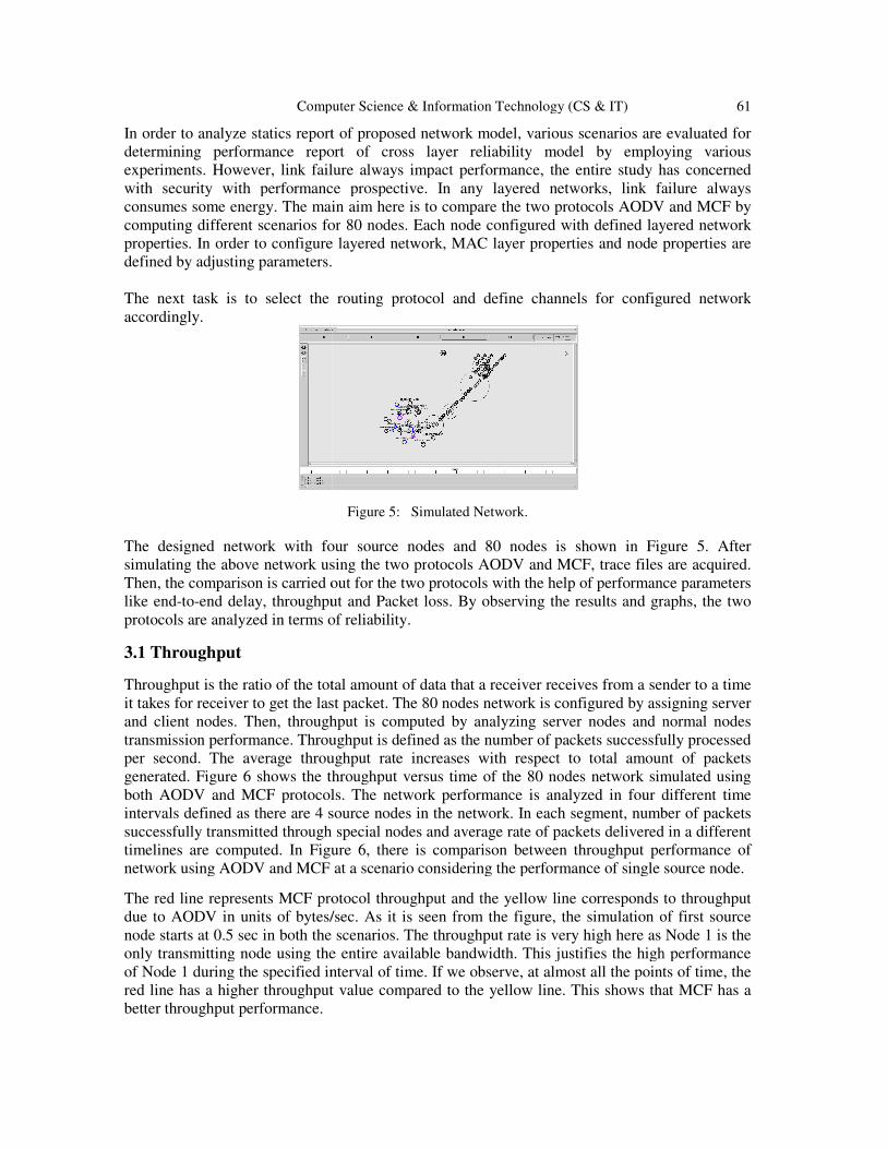
Computer Science & Information Technology (CS & IT)
In order to analyze statics report of proposed determining performance report of cross layer reliability model by employing various experiments. However, link failure always impact with security with performance prospective. In any layered networksconsumes some energy. The main aim computing different scenarios forproperties. In order to configure layered network, defined by adjusting parameters. The next task is to select the routing protocol and define channels for configured networkaccordingly.
The designed network with four source nodes and 80 nodes simulating the above network using the two prThen, the comparison is carried out for like end-to-end delay, throughput and Packet loss. By protocols are analyzed in terms of reliability.
3.1 Throughput
Throughput is the ratio of the total amount of data that a receiver receives from a sender to a time it takes for receiver to get the last packet.and client nodes. Then, throughput transmission performance. Throughput is defined as the number per second. The average throughput rate increases with respect to total amount of packets generated. Figure 6 shows the throughput versusboth AODV and MCF protocols. intervals defined as there are 4 source nodes in the networksuccessfully transmitted through special nodestimelines are computed. In Figure 6network using AODV and MCF at a scenario considering the performance of single source node.
The red line represents MCF protocol throughput and the yellow line corresponds to throughput due to AODV in units of bytes/sec. As it is seen from the figure, the simulation of first source node starts at 0.5 sec in both the scenarios. The throughput rateonly transmitting node using the entire available bandwidth. This justifies the high performance of Node 1 during the specified interval of time. If we observe, at almost all the points of time, the red line has a higher throughput value compared to the yellow line. This shows that MCF has a better throughput performance.
Computer Science & Information Technology (CS & IT)
order to analyze statics report of proposed network model, various scenarios are evaluated determining performance report of cross layer reliability model by employing various
, link failure always impact performance, the entire study has concerned with security with performance prospective. In any layered networks, link failure always
he main aim here is to compare the two protocols AODV and MCF for 80 nodes. Each node configured with defined layered network
configure layered network, MAC layer properties and node properties parameters.
next task is to select the routing protocol and define channels for configured network
Figure 5: Simulated Network.
The designed network with four source nodes and 80 nodes is shown in Figure 5simulating the above network using the two protocols AODV and MCF, trace files
is carried out for the two protocols with the help of performance parameters end delay, throughput and Packet loss. By observing the results and graphs,
in terms of reliability.
ratio of the total amount of data that a receiver receives from a sender to a time it takes for receiver to get the last packet. The 80 nodes network is configured by assigning server
hroughput is computed by analyzing server nodes and normal nodes Throughput is defined as the number of packets successfully processed
The average throughput rate increases with respect to total amount of packets throughput versus time of the 80 nodes network simulated using
both AODV and MCF protocols. The network performance is analyzed in four different time intervals defined as there are 4 source nodes in the network. In each segment, number of packets
gh special nodes and average rate of packets delivered in a different are computed. In Figure 6, there is comparison between throughput performance of
network using AODV and MCF at a scenario considering the performance of single source node.
The red line represents MCF protocol throughput and the yellow line corresponds to throughput due to AODV in units of bytes/sec. As it is seen from the figure, the simulation of first source node starts at 0.5 sec in both the scenarios. The throughput rate is very high here as only transmitting node using the entire available bandwidth. This justifies the high performance of Node 1 during the specified interval of time. If we observe, at almost all the points of time, the
throughput value compared to the yellow line. This shows that MCF has a
61
are evaluated for determining performance report of cross layer reliability model by employing various
study has concerned link failure always
two protocols AODV and MCF by gured with defined layered network
MAC layer properties and node properties are
next task is to select the routing protocol and define channels for configured network
is shown in Figure 5. After trace files are acquired. performance parameters
results and graphs, the two
ratio of the total amount of data that a receiver receives from a sender to a time by assigning server and normal nodes
ckets successfully processed The average throughput rate increases with respect to total amount of packets
network simulated using different time
number of packets and average rate of packets delivered in a different
, there is comparison between throughput performance of network using AODV and MCF at a scenario considering the performance of single source node.
The red line represents MCF protocol throughput and the yellow line corresponds to throughput due to AODV in units of bytes/sec. As it is seen from the figure, the simulation of first source
is very high here as Node 1 is the only transmitting node using the entire available bandwidth. This justifies the high performance of Node 1 during the specified interval of time. If we observe, at almost all the points of time, the
throughput value compared to the yellow line. This shows that MCF has a

62 Computer Science & Information Technology (CS & IT)
Figure 6: Throughput Comparison.
3.2 Packet Loss
At the physical layer of each wireless node, there is a receiving threshold. When a packet is received, if its signal power is below the receiving threshold, it is marked as error and dropped by the MAC layer.Packets Loss is defined as the total number of packets dropped during the simulation. Lower the value of packet loss, better the performance of the protocol. In Figure 7, the red line represents AODV protocol and the blue line corresponds to MCF. The performance graph of a third source node which starts at 30 sec in both scenarios is considered. It is clear that packet loss with AODV protocol is higher than that of MCF protocol. At some points of time, packet loss due to AODV protocol is reaching very high peaks around 140 packets lost. The highest loss is around 100 packets in the case of MCF.
3.3 End to End Delay
The End to End delay is the average time taken by a data packet to arrive at the destination. It also includes the delay caused by route discovery process and the queue in data packet transmission. Only the data packets that successfully delivered to destinations are counted. Average delay = ∑ (arrive time – send time)/∑ Number of connections. The lower value of end to end delay means the better performance of the protocol. The end-to-end delay over a path is the summation of delays experienced by all the hops along the path. In order to compute this metric over a wireless channel, each node needs to monitor the number of packets buffered at the network layer waiting for MAC layer service, as well as measuring the transmission failure probability at the MAC layer. The transmission failure probabilityis the probability that a MAC-layer transmission fails due to either collisions or bad channel quality. Figure 8 shows the end to end delay performance for the 80 nodes network. The red line represents AODV protocol and the blue line corresponds to MCF. As shown from the figure, the performance graph of a third source node which starts at 30 sec is considered for both scenarios. It is clear that end to end delay of packets in the network with AODV protocol is higher than that of MCF. When AODV protocol is used, the peak delay of a packet reaches 700 µ sec where as it is around 550 µ sec in MCF.
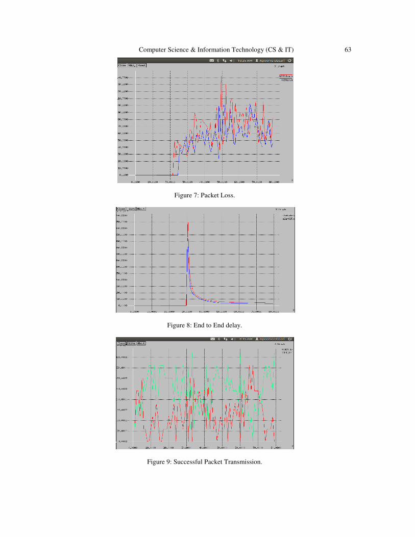
Computer Science & Information Technology (CS & IT) 63
Figure 7: Packet Loss.
Figure 8: End to End delay.
Figure 9: Successful Packet Transmission.

64 Computer Science & Information Technology (CS & IT)
3.4 Successful Packet Transmission:
The trend of successful packet transmission is observed in both the protocols. Figure 9 shows the number of successfully transmitted packets during the simulation time. The green line represents packet transmission in MCF and red line in AODV protocols. At almost all points, MCF has higher successful transmission rate compared to AODV protocol.
4. CONCLUSION
In this paper, Wireless Sensor Network is implemented with AODV and MCF protocols. MCF uses mincut as weight function. Comparison of the performance of both the protocols in terms of different network parameters such throughput, packet loss and end to end delay is carried out. It is observed that in terms of all the network parameters, MCF protocol shows better performance compared to AODV protocol. The comparison in terms of successful packet transmission rate is also observed which showed that MCF protocol has better reliability compared to AODV. Therefore, a more reliable network with better performance can be designed using MCF protocol.
REFERENCES
[1] V. Srivastava and M. Motani, “Cross-layer design: a survey and the road ahead,” Communications
Magazine, IEEE, vol. 43, no. 12, pp. 112–119, 2005. [2] K. Lee, H.-W. Lee, and E. Modiano, “Reliability in layered networks with random link failures,”
MIT, Tech. Rep., 2009. [3] K. Lee and E. Modiano, “Cross-layer survivability in WDM-based networks,” in IEEE INFOCOM,
Rio de Janeiro, Brazil, Apr. 2009. [4] D. Karger, “A randomized fully polynomial time approximation scheme for the all terminal reliability
problem,” SIAM Review, vol. 43, no. 3, pp. 499–522, 2001. [5] W. Su and T. L. Lim, “Cross-layer design and optimization for wireless sensor networks,” in SNPD-
SAWN ’06: Proceedings of the Seventh ACIS International Conference on Software Engineering, Artificial Intelligence, Networking, and Parallel/Distributed Computing, Washington, DC, USA: IEEE Computer Society, 2006, pp. 278–284.
[6] A. Aggarwal, A. Bar-Noy, D.Coppersmith, R. Ramaswami, B. Schieber, and M. Sudan., “Efficient routing in optical networks,”Journal of the ACM, 43(6), November 1996.
[7] Y. Kim, I. Moon and S .Cho, “A comparison of Improved AODV Routing Protocol based on IEEE 802.11 AND IEEE 802.15.4,” Department Of Information Media Engineering, School Of Engineering, Taylor’s University, Vol: 4, No.2(2009), 132-141.
[8] J. S. Provan and M. Ball, “The complexity of counting cuts and of computing the probability that a graph is connected,” SIAM J. Comput., vol. 12, no. 4, pp. 777–788, Nov. 1983.
[9] http://www.ece.ubc.ca/~teerawat/NS2.htm [10] L. Breslau et al., “Advances in network simulation,” IEEE Computer, 33(5):59-67, May 2000. [11] NS-2 tutorials on Youtube. [12] Google forums on NS-2.

Computer Science & Information Technology (CS & IT) 65
AUTHORS Apoora Dasari was born in India in 1991. She received the B. A. Technology Electronics and Communication Engineering degree from Jawaharlal Nehru Technology University, India, in 2012 and M.S degree in Electrical and Computer Engineering from Purdue University, Indianapolis, Indiana in 2014. Her main areas of research interests are networking and wireless communication.
Mohamed A. El-Sharkawy: received the Ph.D. degree in electrical engineering from Southern Methodist University, Dallas, TX, in 1985. He is a Professor of Electrical and Computer Engineering at Purdue School of Engineering and Technology. He is the author of four textbooks using Freescale’s and Motorola’s Digital Signal Processors. He has published over two hundred papers in the areas of digital signal processing and communications. He is a member of Tau Beta Pi and Sigma Xi. He received several million dollars of industrial research grants, supervised large number of graduate theses and consulted for a large number of companies. He received the Outstanding Graduate Student Award from Southern Methodist University. He received the Abraham M. Max Distinguished Professor Award from Purdue University. He received the US Fulbright Scholar Award in 2008. He received the Prestigious External Award Recognition Award from Purdue School of Engineering and Technology, 2009. He is a reviewer for the National Science Foundation and Fulbright.

AUTHOR INDEX
Akitha Kesireddy 35
Apoorva Dasari 55
Chang-Ling Hsu 43
Ekta Walia 27
Eric Ngai 19
Haissam El-Aawar 01
Mohamed El-Sharkawy 35
Mohamed El-Sharkawy 55
Noppon Choosri 09
Vincent Cho 19
Vishal Verma 27