Computer Networks III - Uppsala University
19
http://www.it.uu.se/edu/course/homepage/datakom3/vt11 Partly adapted from www.jochenschiller.de Computer Networks III Wireless Transmission http://www.it.uu.se/edu/course/homepage/datakom3/vt11 Partly adapted from www.jochenschiller.de Radio Spectrum • VLF = Very Low Frequency UHF = Ultra HighFrequency • LF = Low Frequency SHF = Super High Frequency • MF = Medium Frequency EHF = Extra High Frequen • HF = High Frequency UV = Ultraviolet Light • VHF = Very High Frequency 1 Mm 300 Hz 10 km 30 kHz 100 m 3 MHz 1 m 300 MHz 10 mm 30 GHz 100 μm 3 THz 1 μm 300 THz visible light VLF LF MF HF VHF UHF SHF EHF infrared UV optical transmission coax cable twisted pair Frequency and wave length: ! = c/f wave length !, speed of light c " 3x10 8 m/s, frequency f
Transcript of Computer Networks III - Uppsala University
http://www.it.uu.se/edu/course/homepage/datakom3/vt11 Partly adapted from www.jochenschiller.de
Computer Networks III
Wireless Transmission
http://www.it.uu.se/edu/course/homepage/datakom3/vt11 Partly adapted from www.jochenschiller.de
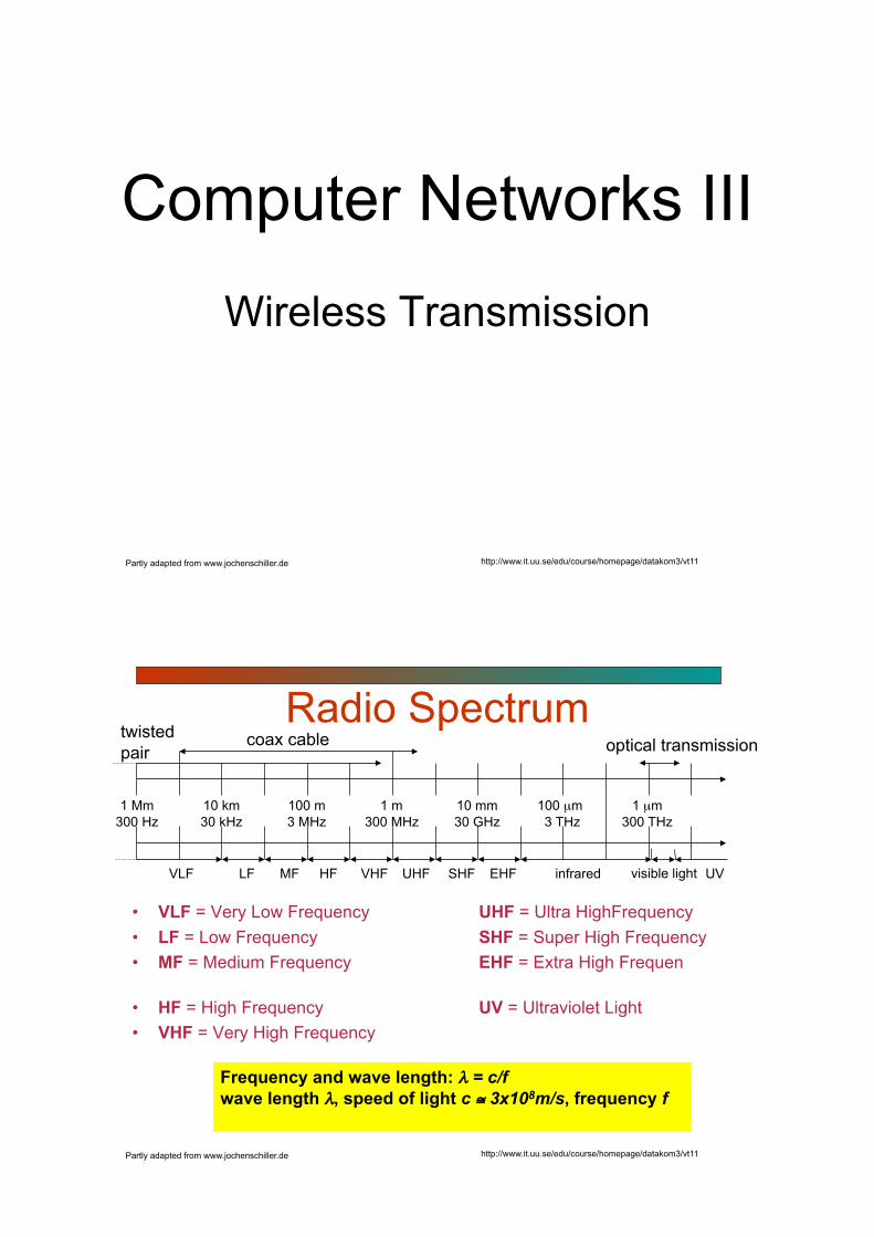
Radio Spectrum
• VLF = Very Low Frequency UHF = Ultra HighFrequency • LF = Low Frequency SHF = Super High Frequency • MF = Medium Frequency EHF = Extra High Frequen
• HF = High Frequency UV = Ultraviolet Light • VHF = Very High Frequency
1 Mm 300 Hz
10 km 30 kHz
100 m 3 MHz
1 m 300 MHz
10 mm 30 GHz
100 µm 3 THz
1 µm 300 THz
visible light VLF LF MF HF VHF UHF SHF EHF infrared UV
optical transmission coax cable twisted pair
Frequency and wave length: ! = c/f wave length !, speed of light c " 3x10⁸m/s, frequency f

http://www.it.uu.se/edu/course/homepage/datakom3/vt11 Partly adapted from www.jochenschiller.de
http://www.it.uu.se/edu/course/homepage/datakom3/vt11 Partly adapted from www.jochenschiller.de
Frequencies(MHz) and regulations Europe USA Japan
Cellular Phones
GSM 450-457, 479-486/460-467,489-496, 890-915/935-960, 1710-1785/1805-1880 UMTS (FDD) 1920-1980, 2110-2190 UMTS (TDD) 1900-1920, 2020-2025
AMPS, TDMA, CDMA 824-849, 869-894 TDMA, CDMA, GSM 1850-1910, 1930-1990
PDC 810-826, 940-956, 1429-1465, 1477-1513
Cordless Phones
CT1+ 885-887, 930-932 CT2 864-868 DECT 1880-1900
PACS 1850-1910, 1930-1990 PACS-UB 1910-1930
PHS 1895-1918 JCT 254-380
Wireless LANs
IEEE 802.11 2400-2483 HIPERLAN 2 5150-5350, 5470-5725
902-928 IEEE 802.11 2400-2483 5150-5350, 5725-5825
IEEE 802.11 2471-2497 5150-5250
Others RF-Control 27, 128, 418, 433, 868
RF-Control 315, 915
RF-Control 426, 868
http://www.it.uu.se/edu/course/homepage/datakom3/vt11 Partly adapted from www.jochenschiller.de
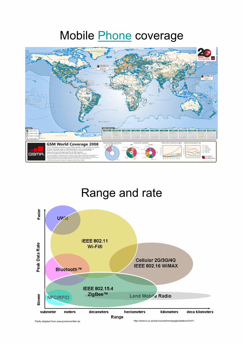
Mobile Phone coverage
http://www.it.uu.se/edu/course/homepage/datakom3/vt11 Partly adapted from www.jochenschiller.de
Range and rate

http://www.it.uu.se/edu/course/homepage/datakom3/vt11 Partly adapted from www.jochenschiller.de
Future Standards
http://www.it.uu.se/edu/course/homepage/datakom3/vt11 Partly adapted from www.jochenschiller.de
• Equal radiation in all directions (three dimensional) – (only a theoretical reference antenna)
• Received power: Pf=Kf1/d2, d=distance, Kf = frequency dependent constant
Antennas: (Ideal) Isotropic radiator z y
x
z
y x

http://www.it.uu.se/edu/course/homepage/datakom3/vt11 Partly adapted from www.jochenschiller.de
Antennas: simple dipoles
Radiation pattern of a simple Hertzian dipole Gain: maximum power in the direction of the
main lobe
side view (xy-plane)
x
y
side view (yz-plane)
z
y
top view (xz-plane)
x
z
simple dipole
!/4 !/2
http://www.it.uu.se/edu/course/homepage/datakom3/vt11 Partly adapted from www.jochenschiller.de
Antennas: directed and sectorized
top view, 3 sector
x
z
top view, 6 sector
x
z
side view (xy-plane)
x
y
side view (yz-plane)
z
y
top view (xz-plane)
x
z
Directed antenna, e.g in a valley
Sectorized antenna, e.g. Mobile phone base station

http://www.it.uu.se/edu/course/homepage/datakom3/vt11 Partly adapted from www.jochenschiller.de
Radio signals • Parameters of periodic signals:
– Period T, – Frequency f=1/T, – Amplitude A, – Phase shift #
s(t) = At sin(2 $ ft t + #t)
• Function of time, location and phase
http://www.it.uu.se/edu/course/homepage/datakom3/vt11 Partly adapted from www.jochenschiller.de
Sine Wave A
s(t) = At sin(2$ ft t + #t)
"
t

http://www.it.uu.se/edu/course/homepage/datakom3/vt11 Partly adapted from www.jochenschiller.de
• Different representations of radio signals – Amplitude (amplitude domain) – frequency spectrum (frequency domain) – phase state diagram (amplitude M and phase " in polar coordinates)
Signals II
f [Hz]
A [V]
"
I= M cos "
Q = M sin "
"
A [V]
t[s]
http://www.it.uu.se/edu/course/homepage/datakom3/vt11 Partly adapted from www.jochenschiller.de
Fourier representation of periodic signals
)2cos()2sin(21)(
11
nftbnftactgn
nn
n !! ""#
=
#
=
++=
1
0
1
0 t t
ideal periodic signal real composition (based on harmonics)
Digital signals need infinite frequencies for perfect transmission => modulation with a carrier frequency for transmission

http://www.it.uu.se/edu/course/homepage/datakom3/vt11 Partly adapted from www.jochenschiller.de
Modulation and demodulation
synchronization decision
digital data analog
demodulation
radio carrier
analog baseband signal
101101001 radio receiver
digital modulation
digital data analog
modulation
radio carrier
analog baseband signal
101101001 radio transmitter
http://www.it.uu.se/edu/course/homepage/datakom3/vt11 Partly adapted from www.jochenschiller.de
Modulation • Digital modulation
– digital data is translated into an analog signal (baseband) – Choice of coding: differences in spectral efficiency, power
efficiency, robustness • Analog modulation
– shifts center frequency of baseband signal up to the radio carrier
• Motivation – Smaller antennas (e.g., !/4) – Frequency Division Multiplexing – allocate different bands – medium propagation characteristics – better at higher
frequencies.

http://www.it.uu.se/edu/course/homepage/datakom3/vt11 Partly adapted from www.jochenschiller.de
Digital modulation
• Amplitude Shift Keying (ASK): – very simple – low bandwidth requirements – very susceptible to interference
• Frequency Shift Keying (FSK): – needs larger bandwidth
• Phase Shift Keying (PSK): – more complex – more robust against interference
1 0 1
t
1 0 1
t
1 0 1
t
http://www.it.uu.se/edu/course/homepage/datakom3/vt11 Partly adapted from www.jochenschiller.de
Advanced Phase Shift Keying • BPSK (Binary Phase Shift Keying):
– bit value 0: sine wave, bit value 1: inverted sine wave
– very simple PSK low spectral efficiency – robust, used e.g. in satellite systems
• QPSK (Quadrature Phase Shift Keying): – 2 bits coded as one symbol – symbol determines shift of sine wave – needs less bandwidth compared to
BPSK – more complex
Q
I 0 1
Q
I
11
01
10
00
11 10 00 01
A
t

http://www.it.uu.se/edu/course/homepage/datakom3/vt11 Partly adapted from www.jochenschiller.de
Quadrature Amplitude Modulation • Quadrature Amplitude
Modulation (QAM): – combines amplitude and
phase modulation – possible to code n bits
using one symbol • 2n discrete levels, n=2 • BUT - bit error rate increases
with n – Signal To Noise Ratio, SNR,
determines n.
0000
0001
0011
1000
Q
I
0010
! a
Example: 16-QAM (4 bits = 1 symbol)
! used in standard 9600 bit/s modems
http://www.it.uu.se/edu/course/homepage/datakom3/vt11 Partly adapted from www.jochenschiller.de
Signal propagation ranges
distance
sender
transmission
detection
interference
• Transmission range – communication possible – low error rate
• Detection range – detection of the signal
possible – no communication
possible (too high error rate)
• Interference range – signal may not be
detected – signal adds to the
background noise
http://www.it.uu.se/edu/course/homepage/datakom3/vt11 Partly adapted from www.jochenschiller.de
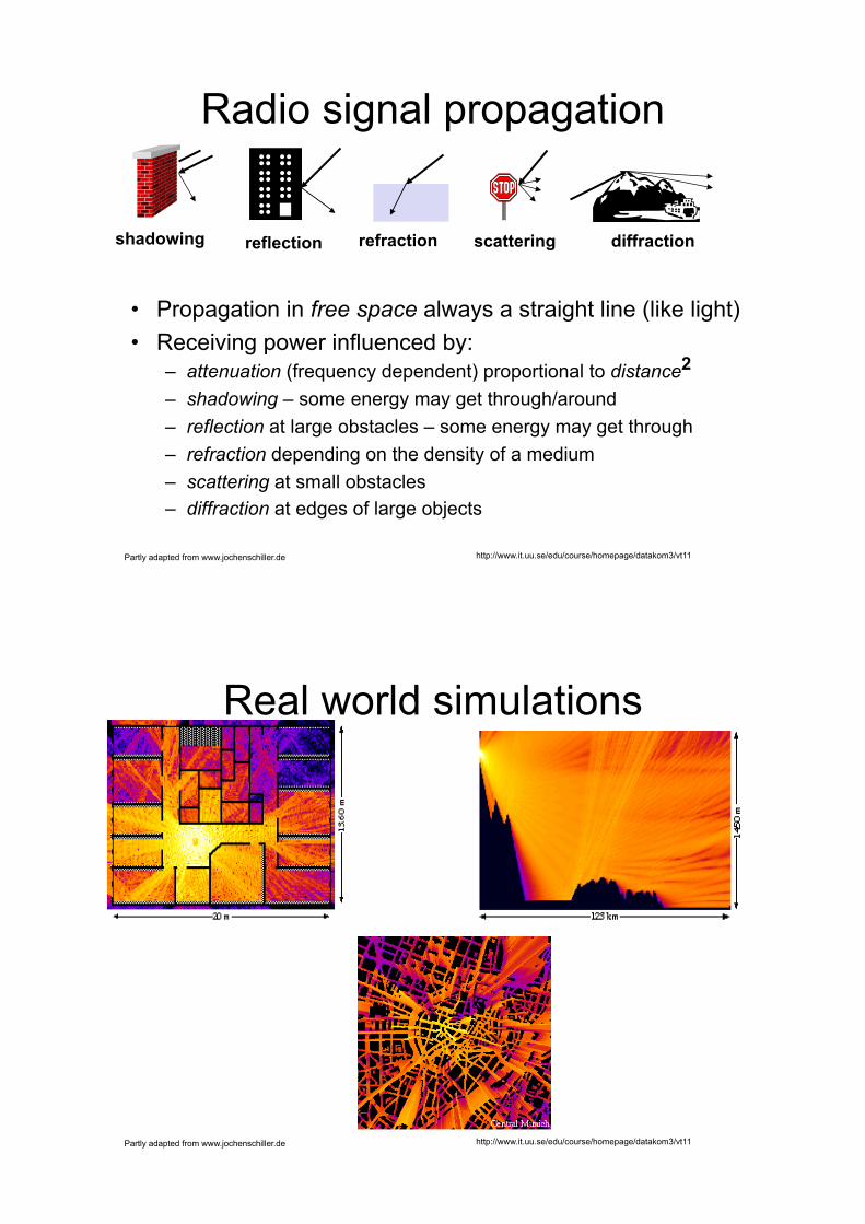
Radio signal propagation
• Propagation in free space always a straight line (like light) • Receiving power influenced by:
– attenuation (frequency dependent) proportional to distance2
– shadowing – some energy may get through/around – reflection at large obstacles – some energy may get through – refraction depending on the density of a medium – scattering at small obstacles – diffraction at edges of large objects
reflection scattering diffraction shadowing refraction
http://www.it.uu.se/edu/course/homepage/datakom3/vt11 Partly adapted from www.jochenschiller.de
Real world simulations

http://www.it.uu.se/edu/course/homepage/datakom3/vt11 Partly adapted from www.jochenschiller.de
• Signal can take many different paths between sender and receiver due to reflection, scattering and diffraction
! interference with “neighbor” symbols, i.e. Inter Symbol Interference (ISI)
Multipath propagation
signal at sender signal at receiver
Line Of Sight pulses
multipath pulses
http://www.it.uu.se/edu/course/homepage/datakom3/vt11 Partly adapted from www.jochenschiller.de
Effects of a moving terminal • Short term, (small scale)
fading – signal paths change – different delay variations of
different signal parts – different phases of signal
parts
• ! quick changes in the power received
• Long term fading – distance to sender – obstacles further away
• ! slow changes in the average power received
short term fading
long term fading
t
power

http://www.it.uu.se/edu/course/homepage/datakom3/vt11 Partly adapted from www.jochenschiller.de
Fading in Ångström corridor
2,4GHZ, IEEE802.15.4
http://www.it.uu.se/edu/course/homepage/datakom3/vt11 Partly adapted from www.jochenschiller.de
High resolution of fading
http://www.it.uu.se/edu/course/homepage/datakom3/vt11 Partly adapted from www.jochenschiller.de
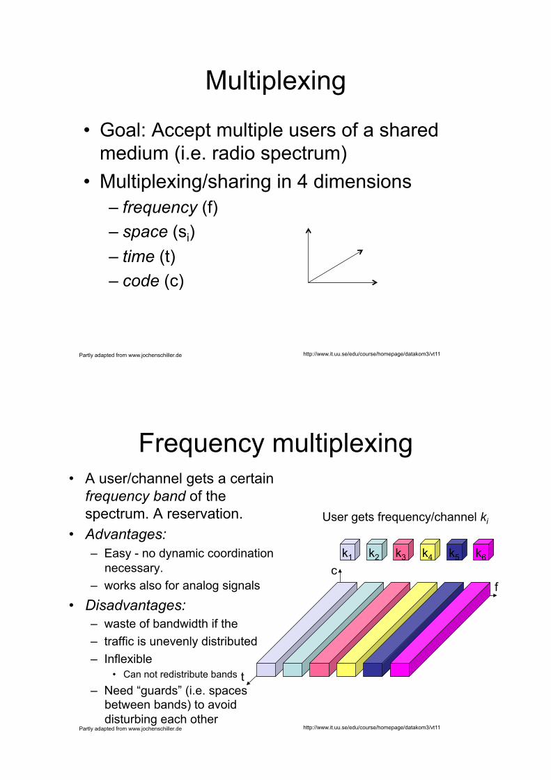
• Goal: Accept multiple users of a shared medium (i.e. radio spectrum)
• Multiplexing/sharing in 4 dimensions – frequency (f) – space (si) – time (t) – code (c)
Multiplexing
http://www.it.uu.se/edu/course/homepage/datakom3/vt11 Partly adapted from www.jochenschiller.de
Frequency multiplexing • A user/channel gets a certain
frequency band of the spectrum. A reservation.
• Advantages: – Easy - no dynamic coordination
necessary. – works also for analog signals
• Disadvantages: – waste of bandwidth if the – traffic is unevenly distributed – Inflexible
• Can not redistribute bands
– Need “guards” (i.e. spaces between bands) to avoid disturbing each other
k2 k3 k4 k5 k6 k1
f
t
c
User gets frequency/channel ki

http://www.it.uu.se/edu/course/homepage/datakom3/vt11 Partly adapted from www.jochenschiller.de
Space Division Multiplexing
s2
s3
s1 f
t c
k2 k3 k4 k5 k6 k1
f
t c
f
t c
Spatial Guard f4 f5
f1 f3
f2
f6
f7
f3 f2
f4 f5
f1
Allocate frequencies in a regular pattern to avoid overlap with same frequency in same geographical area.
User gets frequency/channel ki Transmission ranges of base stations
http://www.it.uu.se/edu/course/homepage/datakom3/vt11 Partly adapted from www.jochenschiller.de
Frequency planning • Frequency reuse only
within a certain distance between the base stations
• Standard model uses 7 frequencies. Distance=3.
• Fixed frequency assignment – Also allow dynamic
frequency planning
f4
f5
f1
f3
f2
f6
f7
f3
f2
f4
f5
f1

http://www.it.uu.se/edu/course/homepage/datakom3/vt11 Partly adapted from www.jochenschiller.de
Space Division Cell structure Mobile stations communicate only via the base station • Advantages of cell structures:
– to get higher capacity, decrease cell sizes and increase density • Cell sizes: City > 100m radius. Country side < 35km radius.
– adaptive transmission power – only needs to reach to the base station.
– Robust against misbehaving clients - centralized control • base station deals with interference, transmission area, etc
• Consequences of cell structures: – fixed network needed for interconnecting base stations – handover (changing from one cell to another, one frequency to
another) is necessary – interference with and between other cells. Requires careful planning.
http://www.it.uu.se/edu/course/homepage/datakom3/vt11 Partly adapted from www.jochenschiller.de
f
t
c
k2 k3 k4 k5 k6 k1
Time multiplexing • A user/channel gets the whole
allocated band for an agreed time-slot t, repeated every nt.
• Advantages: – only one user/channel/carrier in
the medium at any time – utilization high also
for many users • Consequences:
– precise synchronization between distributed nodes necessary
User gets a time-slot ki

http://www.it.uu.se/edu/course/homepage/datakom3/vt11 Partly adapted from www.jochenschiller.de
Combination of time and frequency multiplexing
• A user gets a certain frequency band for a certain amount of time
• Advantages: – protection against frequency
interference – better protection against
eaves listening • Consequence:
– Precise co-ordination required
f
t
c
k2 k3 k4 k5 k6 k1
User gets a time-slot ki (at varying frequencies each time)
http://www.it.uu.se/edu/course/homepage/datakom3/vt11 Partly adapted from www.jochenschiller.de
Code multiplexing
• Each user transmits according to their own unique code on the whole frequency band. – All channels use the same band at the same
time but with different underlying codes.
• Advantages: – no coordination and synchronization necessary – good protection against interference and eaves
tapping (code is protected) – bandwidth efficient – degrades gracefully
• Consequences: – lower user data rates – more complex signal generation
k2 k3 k4 k5 k6 k1
f
t
c
User gets a code ki

http://www.it.uu.se/edu/course/homepage/datakom3/vt11 Partly adapted from www.jochenschiller.de
Spreading and frequency wrt selective fading
frequency
channel quality
1 2 3
4 5 6
narrow band signal
guard space
2 2
2 2
2
frequency
channel quality
1
spread spectrum
narrowband channels
spread spectrum channels
http://www.it.uu.se/edu/course/homepage/datakom3/vt11 Partly adapted from www.jochenschiller.de
Effects of spreading and interference
dP/df
f i)
dP/df
f ii)
sender
dP/df
f iii)
dP/df
f iv)
receiver
f v)
user signal broadband interference narrowband interference
dP/df
dP/df=dPower/dfrequency
spread signal
Narrow band frequency noise
Demodulation spreads noise
Noise impact reduced
receiver
original signal
http://www.it.uu.se/edu/course/homepage/datakom3/vt11 Partly adapted from www.jochenschiller.de
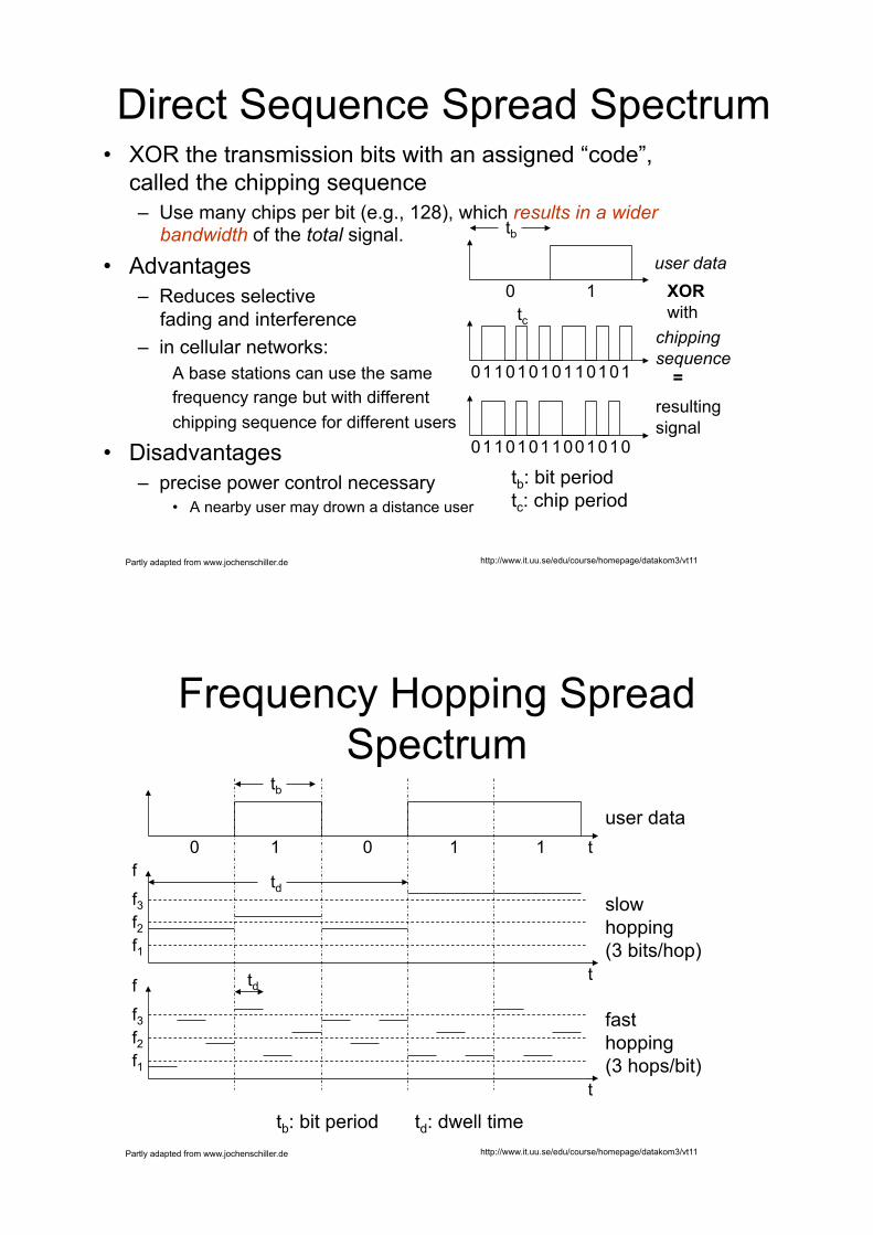
Direct Sequence Spread Spectrum • XOR the transmission bits with an assigned “code”,
called the chipping sequence – Use many chips per bit (e.g., 128), which results in a wider
bandwidth of the total signal.
• Advantages – Reduces selective
fading and interference – in cellular networks:
A base stations can use the same frequency range but with different chipping sequence for different users
• Disadvantages – precise power control necessary
• A nearby user may drown a distance user
user data
chipping sequence
resulting signal
0 1
0 1 1 0 1 0 1 0 1 0 0 1 1 1
XOR with
0 1 1 0 0 1 0 1 1 0 1 0 0 1
=
tb
tc
tb: bit period tc: chip period
http://www.it.uu.se/edu/course/homepage/datakom3/vt11 Partly adapted from www.jochenschiller.de
Frequency Hopping Spread Spectrum
user data
slow hopping (3 bits/hop)
fast hopping (3 hops/bit)
0 1
tb
0 1 1 t f
f1 f2 f3
t
td
f
f1 f2 f3
t
td
tb: bit period td: dwell time