COMPUTER MODEL OF ONE-DIMENSIONAL EQUILIBRIUM CONTROLLED SORPTION

COMPUTER MODEL OF ONE-DIMENSIONAL

EQUILIBRIUM CONTROLLED SORPTION PROCESSES

By David B. Grove and Kenneth G. Stollenwerk

U.S. GEOLOGICAL SURVEY

Water Resources Investigations Report 84-4059

Denver, Colorado

1984

UNITED STATES DEPARTMENT OF THE INTERIOR

WILIAM P. CLARK, Secretary

GEOLOGICAL SURVEY

Dallas L. Peck, Director

For additional informtion write to:

David B. GroveU.S. Geological Survey, MS 413 Box 25046, Federal Center Lakewood, CO 80225

For sale by:

Open-File Services Section Western Distribution Branch U.S. Geological Survey, MS 306 Box 25425, Federal Center Denver, CO 80225

Telephone: (303) 234-5888

CONTENTS

Page

Abstract ............................... 7Introduction ............................. 8Theory ................................ 8

Physical processes ........................ 9Chemical processes ........................ 10

Langmuir adsorption ..................... 16Freundlich adsorption .................... 16Mass-action equilibrium ................... 17

Monovalent-monovalent-exchange ............. 18Divalent-divalent exchange ............... 19Monovalent-divalent exchange .............. 19Divalent-monovalent exchange .............. 20

General linear equation. ..................... 21Numerical-solution techniques ..................... 22Computer program. ........................... 23

General program features ..................... 23Main routine. ........................ 23Subroutines ......................... 24

Evaluation of model results. ................... 25Linear reaction terms .................... 25Non-linear reaction terms .................. 30

References cited ........................... 37Supplemental Data ........................... 38Attachment I. Definition of selected program variables ........ 39Attachment II. Data-input format ................... 42Attachment III. Input data for selected figures. ........... 44Attachment IV. Example of computer output. .............. 46Attachment V. FORTRAN 77 program listing ............... 48

ILLUSTRATIONS

Page

Figure 1. Diagram showing typical isotherms for favorable*linear, and unfavorable sorption. ............ 12

2. Concentration profile of a pulse, at two different times, within a column that has favorable sorption characteristics. ..................... 13

3. Concentration profile of a pulse exiting from a columnwith favorable sorption characteristics. ......... 13

4. Concentration profile of a pulse, at two different times, within a column that has a linear-sorption isotherm ......................... 14

5. Concentration profile of a pulse exiting from a columnthat has a linear-sorption isotherm. ........... 14

6. Concentration profile of a pulse, at two different times, within a column that has an unfavorable- sorption isotherm. .................... 15

7. Concentration profile of a pulse exiting from a columnthat has an unfavorable-sorption isotherm. ........ 15

8. Graph showing comparisons of model and analytical solutions to the convective-diffusion equation for Brenner numbers of 2 and 20 for a step input ....... 26

9. Graph showing comparisons of model and analytical solutions to the convective-diffusion equation for Brenner numbers of 2 and 20 for a pulse input. ...... 27

10. Graph showing a comparison of model and analytical solutions for linear sorption and first-order irreversible-rate reactions. ............... 29

11. Graph showing a comparison of model and analyticalsolution for column throughput with Langmuir sorptionfor various values of input concentration. ........ 32

12. Graph showing a comparison of model and analyticalsolutions for column throughput with Freundlich sorptionfor various values of the Freundlich exponent. ...... 33

13. Graph showing a comparison of model and analytical solutions for column throughput with sorption represented by mono-monovalent ion exchange for various values of input concentration. .......... 34

14. Graph showing a comparison of model and analytical solutions for column throughput with sorption represented by mono-divalent ion exchange for various values of input concentration. .......... 35

15. Graph showing a comparison of model and analytical solutions for column throughput with sorption represented by di-monovalent ion exchange for various values of input concentration. .......... 36

TABLES

Page

Table 1. Physical properties used in sorptive model tests ...... 282. Chemical parameters used for column runs .......... 30

COMPUTER MODEL OF ONE-DIMENSIONAL

EQUILIBRIUM-CONTROLLED SORPTION PROCESSES

By

David B. Grove and Kenneth G. Stollenwerk

ABSTRACT

A numerical solution to the one-dimensional solute-transport equation with equilibrium-controlled sorption and a first-order irreversible-rate reaction is presented. The computer code is written in FORTRAN 77 language, with a variety of options for input and output for user ease. Sorption reactions include Langmuir, Freundlich, and ion-exchange, with or without equal valence. General equations describing transport and reaction processes are solved by finite-difference methods, with non- linearities accounted for by iteration. Complete documentation of the code, with examples, is included.

INTRODUCTION

The solution of one-dimensional solute transport and reaction equations for flow through porous media has been used to analyze and predict results from laboratory columns and from field experiments. In many cases, equations describing the process are so complex that numerical methods are the most effective means of solution. Even when analytical solutions are available, numerical methods may present the required output in the most reasonable manner; therefore, a general numerical solution to these equations has been developed and is presented herein.

The solute-transport and reactions equation is solved by using a finite-difference method. A variety of input conditions can be simulated, including both pulse and step input, with either flux continuity or constant-concentration boundary conditions. Chemical reactions can be homogeneous, heterogeneous, or both. The homogeneous reaction is a first- order irreversible kinetic expression, such as radioactive decay, with or without the presence of sorption, (a term used for both adsorptive and ion- exchange reactions). The heterogenous reaction represents sorption processes and can be simulated by using the mass-action ion-exchange equation or the Langmuir or Freundlich adsorption equations. All sorption processes are assumed to be equilibrium-controlled during their reaction step.

THEORY

When solute transport is simplified to one dimension, computation becomes easier. The differential equation that describes this transport has only two independent variables: time and distance. The dependent variables in this equation include concentration of the solute in the liquid phase, and, in the case of sorption, concentration of the solute on the solid (the sorbed phase). To solve this equation, additional equations need to be available to define the relationship between dissolved and sorbed phases.

The one-dimensional defining differential equation can be taken from Grove and Rubin (1977) as:

8 dc + 8y dc _ eD d_c = CREW, (1) dt dx A J2

where

e is the effective porosity;c is the concentration of the solute (mass of solute/volume of

liquid), ML"3 ; t is the time variable, T;V is the interstitial fluid velocity, LT"1 ; x is the distance variable, L; and D is the coefficient of hydrodynamic dispersion, LrT"1 ;

when CHEM equals - p^ ^£ for equilibrium-controlled adsorption andexchange reactions, and

-k(ec + PI,C) for first order irreversible-rate reactionswith equilibrium controlled ion exchange or adsorption, and

_a where p^ is the bulk density of the porous medium, ML ;

c is the concentration of the species adsorbed on the solid, MM'1 ;and

k is the rate constant for the kinetic reaction,

The initial conditions in the column are given as

c(x,t = 0) = C

The input boundary conditions may be either described by flux continuity

D 4s- = - V(c - C,) for x = 0 at t, A-* idx

or a constant concentration

c = C i for x = 0 at t

The output boundary condition is given as

c = 0 for x = L at t dx

_3 where C^ is the input concentration of the solute, ML ,

G£ is the initial concentration of the solute in the column, ML ;and

L is the length of the column, L.

A discussion of these boundary conditions is given in detail by Dankwerts (1953).

The above solute-transport equation (equation 1) contains physical and chemical terms that will now be discussed in more detail. The most notable are the terms defining the chemical reactions, both equilibrium- controlled and kinetically controlled and the dispersion term. Physical processes that include dispersive and convective fluxes will be discussed first.

Physical processes

The second term on the left-hand side of equation 1 describes the convective flux and the third term on the left-hand side of equation 1

describes the dispersive flux. The convective flux is described by the product of the velocity and concentration. Velocity can be determined in a number of ways: (1) It can be determined independently knowing the volumetric-flow rate and the column's physical characteristics (length, diameter, and porosity), or (2) it also can be determined by introducing a conservative (non-reacting) solute and matching a solution of equation 1 for various values of velocity and dispersivity, until a best fit between experimental results and theoretical prediction is obtained.

The dispersive flux is computed as the product of a dispersion coefficient D and the concentration gradient. This flux is assumed to consist of two components; mechanical dispersion and molecular diffusion. In the accompanying computer program it is described as:

D = aV + D, (2)

where a is the characteristic dispersive length, L; andD is the product of the molecular diffusion coefficient and the

tortuosity, LT"1 .

For most field situations mechanical dispersivity overshadows molecular diffusion to the extent that the latter can be neglected (see as examples Bear, 1972, p. 358 and Freeze and Cherry, 1979, p. 390). The dispersion coefficient usually is determined by introducing a conservative tracer into the column and matching a solution to equation 1 with experimental results. Small values of the dispersion constant, or approximations of larger values, can be calculated as described in Levenspiel (1972, p. 280).

Chemical processes

One of the most common and frequently modeled type of chemical reaction occurring during the movement of solutes through porous media is sorption of the solute onto the solid surface through a physical attraction or an exchange process. When movement of the solute is slow, compared to the adsorption or exchange reaction rate, it is assumed to be equilibrium- controlled, greatly simplifying analysis. This can be illustrated as follows:

dc _ dc dca . T~~ TT*dt dc dt

where is simply the slope of the sorption isotherm of c versus c. dc

The sorption isotherm is defined as a plot of the sorbed phase versus the dissolved phase. Plots are sometimes in terms of relative concentrations, mass fractions, mole fractions, and so forth. The important thing to keep in mind is that the units need to be consistent, and care needs to be taken when transferring data from sorption-isotherm plots to be used with

10

transport-equation calculations. These sorption isotherms can have a variety of shapes; see for example, Vermeulen (1973, chap. 16, p. 14). However, they usually are defined in terms of favorable or unfavorable isotherms. A favorable isotherm is convex-upward and an unfavorable isotherm is concave-upward. Examples of each case are shown in figure 1. If the sorption process is taking place throughout the full range of concentration, it is evident that the slope of the isotherm is changing, and it can be expressed as a function of dissolved concentration. Favorable isotherms have an increasing slope with decreasing concentrations^ and unfavorable isotherms have a decreasing slope with increasing cooncentrations. This explains the shape of pulses passing through chromatographic columns. Sharp breakthrough fronts are obtained from favorable isotherms; diffuse breakthrough fronts are obtained from unfavorable isotherms. When the slope of the isotherm is constant, a pulse of solute travelling through a column should be unchanged in shape, except for a flattening from the effect of dispersion. Note that the terms favorable and unfavorable refer to the sorption of the solute. Elution from the column has the opposite effect and an isotherm that is favorable for sorption is unfavorable for elution. Examples of pulses within a column and exiting from a column for sorption isotherms that are favorable, linear, and unfavorable are shown in figures 2-7. One should note that dispersion in the columns not only causes the pulse to flatten; but, as shown for the case of the linear isotherm, the pulse only stays symmetric within the column. The dispersion process causes a tail to occur in the breakthrough curve that should not be mistaken for adsorption with a favorable isotherm. When sorption processes do occur, the breakthrough curve usually is displaced several pore volumes, when compared to a non- reacting solute.

Now one merely needs a quantitative relation between c and c to evaluate the slope of the isotherm. There are a variety of ways to describe this isotherm or equation, that relate the concentration on the solid in equilibrium with the concentration in solution. Three of the most common expressions used are the Langmuir and the Freundlich adsorption equations, and the mass-action equilibrium relationship for ion exchange. These three equations and a quantitative description of their use in the mass-transport equation will be given in the next section.

A second common chemical process is that of an irreversible first- order rate reaction, such as radioactive decay. In this code, it is assumed that this reaction occurs for both sorbed and dissolved chemical species, it is written:

CHEM = - k(ec + Pb c). (4)

Radioactive decay is well known to be a first-order irreversible-rate reaction. The rate constant k is, by convention, given the symbol, X, and through its definition is shown to be:

In2 X = (5)

11

Zl

TjH-

OQ

RELATIVE SORBED CONCENTRATION

fl> OQ

* a

& v> » >-T<

O 9

mi- >H

m g0) 0)O

m oo Oz o mz

H

OZ

z o

LJLJ OZO OLJU

LJU QC

RELATIVE COLUMN LENGTH

Figure 2. Concentration profile of a pulse, at two different times, within a column that has favorable sorption characteristics.

PORE VOLUMES

Figure 3. Concentration profile of a pulse exiting from a column with favorable sorption characteristics.

13

fl M-

OQ

RE

LA

TIV

E

CO

NC

EN

TR

AT

ION

o

-*

(3*

O

P

0

rt

O O|3

* »

»

rt

W

H S»

P>

rt M-

H»

O

H

O\

M,

(A

M>

O

K*

H

O*d r+

O

H.

M,

O

»-*

r+

M

(3*

O

O H

<6

9

M OQ

O 33 m < O i-

c

s m 0)

OQ 0

H

RE

LA

TIV

E

CO

NC

EN

TR

AT

ION

C»

M.

Oo

B

»rf

«

O(3

* OT

fl)

rt

rt13

* H

.M

. O

tl

3

B> fcr*

05 fl)

rtP»

4

H

O

rt

<6H

. H

O

fl>

3) m m o

O i-

c

S

z I-

m

z

o

-I

I

z tu o z o otu

tu

= Tf

FLOW T = T

RELATIVE COLUMN LENGTH

Figure 6. Concentration profile of a pulse, at two different times, within a column that has an unfavorable sorption isotherm.

PORE VOLUMES

Figure 7. Concentration profile of a pulse exiting from a column that has an unfavorable-sorption isotherm.

15

where

X is the rate constant k, T~* ;In 2 is the natural logarithm of 2; and

* s *ke radioactive half-life of the element, T.

Langmuir adsorption

The equation that describes Langmuir adsorption is given as;

c = (6) 1 + Kjc

where Ki is the adsorption equilibrium constant, and Q is the maximum number of adsorption sites.

The terms Kj and Q can be evaluated from plots of experimental data of 1/c versus 1/c. If Langmuir adsorption applies, this should result in a straight line with slope l/(KjQ) and intercept 1/Q. The slope of the Langmuir isotherm is given as:

-- __ dc 2

For small concentrations, slope is given by the constant, KQ.

Freundlich isotherm

The equation that describes the Freundlich isotherm is given by

c = Kfcn (8)

where Kf is the Freundlich adsorption equilibrium constant,and n is the Freundlich exponent.

The terms K^ and n can be evaluated from plots of experimental data of In c versus In c. If a Freundlich isotherm applies, this should result in a straight line with a slope of n and an intercept of In K.

16

The slope of the isotherm is given as:

=nKfCn-. (9) dc r

When the exponent n is equal to one, the slope is linear (constant), independent of the concentration and equal to Kf.

Mass-action equilibrium

Four types of ion-exchange processes will be considered, depending on the values of m and n for the equation:

n _ >- _ mme + nc < me + nc (10)12 12

where n is the valence for ion 1, and, m is the valence for ion 2.

The ion-exchange selectivity coefficient for equation 10 is defined as:

-m _n c l C2

when the total-solution concentration and ion-exchange capacity are constant, and only two ions are involved, we can write:

nc. mc2 = CQ , and (12)

\ + mc2 = Q. (13)nc

Typical units of concentration for dissolved and sorbed species would be, moles per liter for c^ and c 2 > an<* millimoles per gram c^ and c~2> Units for the total concentration, CQ , would then be equivalents per liter and units for the cation-exchange capacity, Q, would be millequivalents per gram. Equations 12 and 13 will be substituted into equation 11 in order to eliminate component 2 from the equation. The slope of the ion-exchange isotherm can then be computed.

17

Monovalent mpnovalent exchange

In this example both ions have a valence of one (n = m = 1). A typical example might be the exchange of sodium and potassium,

Na+ + KX NaX + K+ (14)

using equations 11, 12, and 13, the equilibrium concentration of adsorbed sodium would be:

c = - . (15) ) + C0

Both concentrations shown are of sodium as the potassium concentrations have been eliminnated through the use of equations 12 and 13. Equation 15 can be used to construct the ion-exchange isotherm for sodium, for this particular system. Dissolved and adsorbed equilibrium concentrations of potassium can be calculated using equations 12 and 13.


^ = ^-. (16) dc

When IL. = 1, or for small values of c, the slope becomes:

^ = . (17) dc C0

When the slope of the isotherm, whether exchange or adsorption, is linear, either because of the value of the equation coefficients or because of relatively small concentrations of the solute of interest, it has been termed the distribution coefficient, and sometimes given the value KJ. One should note that, in this case, the distribution coefficient is affected significantly by the total-solution concentration. As the total-solution concentration increases, the distribution coefficient decreases, as a result of computation of the counter ion for the exchange sites. Some authors (Helfferich, 1962, p. 154) define the distribution coefficient as the ratio of the adsorbed to the dissolved ions. This would be equal to the slope of the isotherm only for linear isotherms.

18

Divalent-divalent exchange

In this example both ions have a valence of two (m = n = 2). A typical example might be the exchange of calcium and strontium.

Ca++ + SrX ^ CaX + Sr++ (18)

The equilibrium concentration of adsorbed calcium would be:

c = . (19) 2c(Km-l) + C0


^ = -. (20,dc rirfir -i) + r 1 LZCVISn ' co

K m = 1 or for small values of c the limiting value for the slope is the same as for the mono-monovalent exchange, that is equation 17.

Monovalent-divalent exchange

In this example ion 1 has a valence of one and ion 2 has a valence of two (n = 1, m = 2). An example would be the exchange of sodium and calcium

2 Na+ + CaX « 2 NaX + Ca^. (21)

19

The equation that could be used to calculate the equilibrium concentration of adsorbed sodium is:

c 2 (C -c ) + c (K^c 2 ) - K Oc 2 = 0, (22)

which can be solved for c by the solution procedure for a quadratic equation. The isotherm slope is given by:

dc = c2 - oloK, + 2cKmQ

dc 2c(C0-c) + c2^

where the value for c can be obtained from equation 22 in terms of c. For small concentrat slope reduces to:small concentrations of ion 1, such that c « Q, and c «C0 , the isotherm

(24)

Pivalent-monovalent exchange

In this example ion 1 has a valence of two and ion 2 has a valence of one (n = 2, m = 1). While this may seem a trivial extension of the previous monovalent-divalent case, a separate solution is included for user ease. An example similar to equation 21 for calcium sodium exchange would be:

Ca++ + 2 NaX ^2 Na+ + CaX (25)

The equation that could be used to calculate the equilibrium concentration of adsorbed calcium is:

c 2 (4Kmc) + c(-4KmQc - (CQ-2c) 2 ) + K^c = 0, (26)

20

which can be solved for c by the solution procedure for a quadratic equation. The slope of the isotherm is given by:

- 4c(Cn-2c) -(27)

« ) ~ (c0~2c > 2

where the value of c can be obtained from equation 27 in terms of c. For small concentrat slope reduces to:small concentrations of ion 1, such that c^ « Q and c^ « CQ, the isotherm

(28) dc 2

General linear equation

The previously discussed chemical-reaction terms can be incorporated into equation (1) in the following manner: Assume that during its transport, a chemical species is disappearing by some first-order irreversible reaction, and that it is being exchanged reversibly by an equilibrium-controlled process in which the exchange isotherm is linear, and its slope can be represented by the distribution coefficient (described previously). Equation (1) can now be written:

= eD i - eV

K p - ekc(l + -^-b-). (29)

A retardation factor R^, which usually is used in equilibrium-controlled, trace-exchange reactions, can be defined as:

Rf = 1 + Kdpb /e. (30)

21

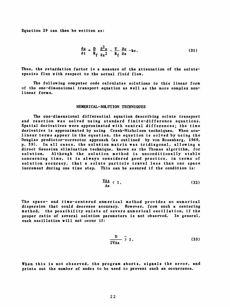
Equation 29 can then be written as:

-kc - < 31 >at R* - ' ~ '

Thus, the retardation factor is a measure of the attenuation of the solute- species flux with respect to the actual fluid flow.

The following computer code calculates solutions to this linear form of the one-dimensional transport equation as well as the more complex non linear forms.

NUMERICAL- SOLUTION TECHNIQUES

The one-dimensional differential equation describing solute transport and reaction was solved using standard finite-difference equations. Spatial derivatives were approximated with central differences; the time derivative is approximated by using Crank-Nicholson techniques. When non linear terms appear in the equation, the equation is solved by using the Douglas predictor-corrector approach (as outlined by von Rosenberg, 1969, p. 59). In all cases, the solution matrix was tridiagonal, allowing a direct Gaussian elimination technique, known as the Thomas algorithm, for solution. Although the solution method is unconditionally stable concerning time, it is always considered good practice, in terms of solution accuracy, that a solute particle travel less than one space increment during one time step. This can be assured if the condition is:

< 1. (32) Ax

The space- and time-centered numerical method provides no numerical dispersion that could decrease accuracy. However, from such a centering method, the possibility exists of severe numerical oscillation, if the proper ratio of several solution parameters is not observed. In general, such oscillation will not occur if:

(33)

When this is not observed, the program aborts, signals the error, and prints out the number of nodes to be used to prevent such an occurrence.

22

A number of alternative-solution techniques can lessen the impact of the above restrictions; the most notable technique is the use of finite elements, using the Galerkin method (Grove, 1977). The author has found that, for one-dimensional problems, enough nodes can be used with finite- difference methods to overcome any oscillation problems without taxing computer storage and time requirements. The use of integration techniques, such as finite elements, thus, is not necessary for most one-dimensional cases. When continuous derivatives are necessary at node locations and boundaries, some investigators have found it necessary to use finite elements with higher-order (cubic) basis functions.

COMPUTER PROGRAM

General program features

The computer program is written in FORTRAN 77 and is operational on the USGS PRIME minicomputer. As this program is not expected to place much of a demand on most computers for core storage, no great attempt has been made to optimize the size of the program. If storage does present a problem, as it might in the case of a small microcomputer, the user simply has to redimension the arrays to the minimum value necessary for program operation. All arrays are presently dimensioned to 101, which allows the user to use as many as 101 nodes in a problem. The program is modular in concept ; it consists of a main program, eight subroutines, and a function program; all variables are passed as arguments. A description of the program follows.

Main routine

The main routine of the program provides the instructions for reading the input data, selects the type of computation and printout requested, and calls the various subroutines that compute the new concentration at the new time step. The input is assumed to be on disk; and is written in free- field format. File input and output names are requested at the console during program execution. This input is separated into three groups. The first group defines the number of nodes, time increment, input boundary conditions, and the kind of output that will be printed. The number of nodes dictates the node spacing. The time increment and velocity defines the distance that a solute will travel in one time step (iteration). The user can fix this parameter or can define a dimensionless group (CDELT) that is the fractional distance between nodes that a solute particle with or without reaction will travel per time step. A new time increment based on this fraction is then computed and used in the program. A value of 0.2 has been determined to be satisfactory for CDELT. Input boundary conditions of constant concentration or constant flux can be specified. Some analytical solutions to the solute transport and reaction equation assume constant-concentration boundary conditions. They also may assume columns of infinite length. When matching computed solutions to analytical solutions of this type, a longer-than-normal column can be used, with output printed out at an interior node. The code automatically corrects for column length, for such printouts as pore volumes are based on a column of the length at the location of the interior node. For matching actual

23

column experimental data, the flux-boundary condition is applicable. The user has the option to print the concentration at any one selected node in the column as a function of pore volume throughput at that node or at preselected nodes within the column as a function of column distance where the pore volume is a function of total column length. Printout of selected data to a disk unit is available for possible graphing purposes. Both of the above printouts occur at user-selected, incremental, pore-volume-output intervals and computation ceases at a specified number of pore-volume output.

The second group of data inputs the fixed physical characteristics of the column, the porous media and the solute. This includes the duration of input pulse, length of column, interstitial velocity of fluid, molecular-diffusion coefficient, mechanical dispersive-characteristic length, bulk density of porous media and effective porosity.

The third group of input data contains information about the possible chemical reactions. This group includes:

1. The type of adsorption or ion exchange that may occur,2. The input solute concentration,3. The use of and value for a linear isotherm (distribution

coefficient),4. The sorptive capacity of the porous media,5. The total solution concentration (for ion exchange),6. The first order irreversible-rate constant,7. Equilibrium coefficients and exponents for Langmuir and Freundlich

adsorption isotherms, and equilibrium ion-exchange isotherms.

The mass-balance calculation computes and outputs the following: total input, total output, loss through chemical reaction, quantity in pores, quantity sorbed, and a fractional error for the cumulative run. Although a small fractional error does not guarantee an accurate solution, a large one certainly indicates a problem.

Subroutines

Besides supplying input, output and mass-balance calculations MAIN directs the computations to the various subroutines. Eight subroutines and one function routine are included in the code. The subroutines FREUN, LANG, EXC, EXCM, and EXCD calculate the coefficients specific to each of the sorption processes mentioned earlier.

The subroutine REACT uses the previously calculated coefficients to compute the concentration at the new time step. Options are available to skip nonlinear computations, when only linear reactions are occurring. When non-linearities have to be taken into account, non-linear coefficients are calculated at TIME + DELT/2, using values at the old time step. Computations at the required TIME + DELT then use this precomputed value. Only one iteration is used, and smaller time steps are neded if greater accuracy is required. The set of linear-algebraic equations that results is solved by the subroutine TRIMAT. A function-subroutine QUADX also is used for solution of the quadratic equation that results from the unequal

24

valence equilibrium reaction, when solution for the concentration in the solid phase is necessary. Selected example problems are illustrated. The program has been written so that output is presented in a format that is no more than 80 columns wide, suitable for most terminal uses.

Evaluation of model results

Evaluation of model results could be done on a firm basis for only a few cases. The use of analytical expressions to test the model is the most common verification procedure, however, these analytical solutions only are available for linear systems. This means that equations that contain certain chemical reactions, such as linear sorption isotherms and first- order reactions can be solved analytically, but the more complicated systems cannot. In cases like the latter, solutions where the isotherms approach linearity, and the mass balances of the solute species can be checked. However, the user needs to be skeptical of the results when theoretical output seems to contradict expected results.

Because the analytical solution used for comparison purposes was developed for a semi-infinite column, and the finite-difference computer solution was developed for a fixed-length column, some means was necessary to compare one with the other. This was accomplished by selecting a point within the column that should not be affected by the concentration leaving the column at that particular time. The pore volume throughout, concentration profile, and so forth, were then based on this interior point. A position halfway up the column normally was used.

Linear reaction terms

The analytical solution to equation 1 with flux boundary conditions and no chemical reactions is presented by Brenner (1962). In this paper, Brenner gives dimensionless concentration as a function of dimensionless time (pore volume) for various values of the Brenner number (VL/4D). Results for Brenner numbers of 2 and 20 illustrating examples with relatively large and relatively small dispersive mixing during transport are shown in figure 8. Theoretical values of Brenner are shown by the solid lines,and results from this computer code are shown by the open circles. An excellent agreement is shown. These first values and the analytical solution were for the flux-boundary condition. The solid circles represent the same runs with constant concentrations. Note that, for this case of significant dispersion, this boundary condition does not give a good result. When moderate values of dispersion are present, the use of a flux-boundary condition is needed. In fact, the use of any other boundary condition only is appropriate when checking the code with analytical solutions using that particular boundary condition. A similar comparison of Brenner numbers of 2 and 20 is shown in figure 9, except that a pulse of one pore volume is input, rather than the step input as illustrated in figure 8. The analytical solution for a pulse is obtained by subtracting one step input from another, after a time corresponding to a pulse input.

25

RELATIVE CONCENTRATION

O

fopCD

O 00

H- OQ

00

W w OH O H0) t > p» d<i> H-H O

tJ

0

fro 0 o> toS ?e

o o0 o I

O V

M§ H. fa n v>H O O

§-n:S10 "1

O H>H H»

*d

w, O H

I I I I I I

o Om

O

2 m


H O H O I p

O H- HOW

p! B or4 o

OCFQ

O o0 « B ** o *

o pN> O H

« H'P 9 w

B *" pM rt p"2 H- H-£ O V!

l-t> OO P

OJ)m< rol-OI- c

m̂

When linear sorptibn and a first-order irreversible-rate reaction are both present, equation 31 results, and the solution is given by Bear (1972, p. 630) as follows:

'2 '1/2C(x,t) = 1/2 Co exp(Vx/2D)[exp(-xp)erfc x - (V z+4kD ) t

2(D't) 1/2(35)

exp(xp)erfc * +2(D't) 1/2

wherefj

P2 = -V- + ^7 , V = V/Rf and D' = D/Rf . 4D2 D

Agreement with the analytical solution and the computer solution for values of k of 0 and 0.01, and isotherm slopes of 0 and 0.3, is shown in figure 10 to be excellent in all cases. Physical properties used in these tests are given in table 1. Using these values, an isotherm slope of 0.3 results in a retardation coefficient of 2.29.

Table 1. Physical properties used in sorptive-model tests

Number of nodes in column (NI)

Column length (XL)

Fluid velocity (V)

Molecular diffusion coefficient (D)

Characteristic length (ALPHA)

Bulk density (RHOB)

Porosity (POR)

Duration of fluid pulse (DPUL)

51

8 centimeters

0.1 centimeters per second

0

1.0 centimeter

1.587 grams per cubic centimeter

0.37

160 seconds

28

Tl

I T

1 I

' '

' '

I '

' '

-

AN

AL

YT

ICA

L S

OLU

TIO

N

NU

ME

RIC

AL

S

OLU

TIO

N

K

RA

TE

C

ON

ST

AN

T

RF

R

ET

AR

DA

TIO

N

FA

CT

OR

K =

0.0

R

F =

2.2

9

PO

RE

V

OLU

ME

Fig

ure

1

0.

Gra

ph

sh

ow

ing

a co

mpar

ison

of

mo

del

an

d an

aly

tical

solu

tions

for

lin

ear

sorp

tion

and fi

rst-

ord

er

irre

vers

ible

-rate

re

acti

ons.

Non-linear reaction terms

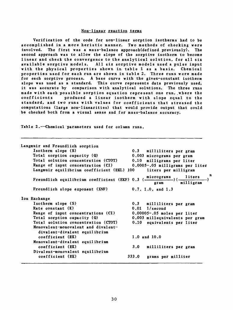
Verification of the code for non-linear sorption isotherms had to be accomplished in a more heristic manner. Two methods of checking were involved. The first was a mass-balance approach(defined previously). The second approach was to allow the slope of the sorptive isotherm to become linear and check the convergence to the analytical solution, for all six available sorptive models. All six sorptive models used a pulse input with the physical properties shown in table 1 as a basis. Chemical properties used for each run are shown in table 2. Three runs were made for each sorptive process. A base curve with the given-constant isotherm slope was used as a standard. This curve represents data previously used, it was accurate by comparison with analytical solutions. The three runs made with each possible sorption equation represent one run, .where the coefficients produced a linear isotherm with slope equal to the standard, and two runs with values for coefficients that stressed the computations (large non-linearities) that would provide output that could be checked both from a visual sense and for mass-balance accuracy.

Table 2. Chemical parameters used for column runs.

Langmuir and Freundlich sorption Isotherm slope (S) Total sorption capacity (Q) Total solution concentration (CTOT) Range of input concentration (CD

0 0 0 0

Langmuir equilibrium coefficient (EEL) 100

.3 milliliters per gram

.003 micrograms per gram

.10 milligrams per liter

.0005-.05 milligrams per liter liters per milligram

.3 (micrograms

Freundlich equilibrium coefficient (EKF) 0

Freundlich slope exponent (XNF) 0.7, 1.0, and 1.3

gramliters

milligram

Ion ExchangeIsotherm slope (S) Rate constant (E)Range of input concentrations (CD Total sorption capacity (Q) Total solution concentration (CTOT) Monovalent-monovalent and divalent-

divalent-divalent equilibrium coefficient (EE)

Monovalent-divalent equilibriumcoefficient (EE)

Divalent-monovalent equilibrium coefficient (EE)

0.3 milliliters per gram 0.01 I/second 0.00005-.05 moles per liter 0.003 millequivalents per gram 0.10 equivalents per liter

1.0 and 10.0

3.0 milliliters per gram

333.0 grams per milliter

30

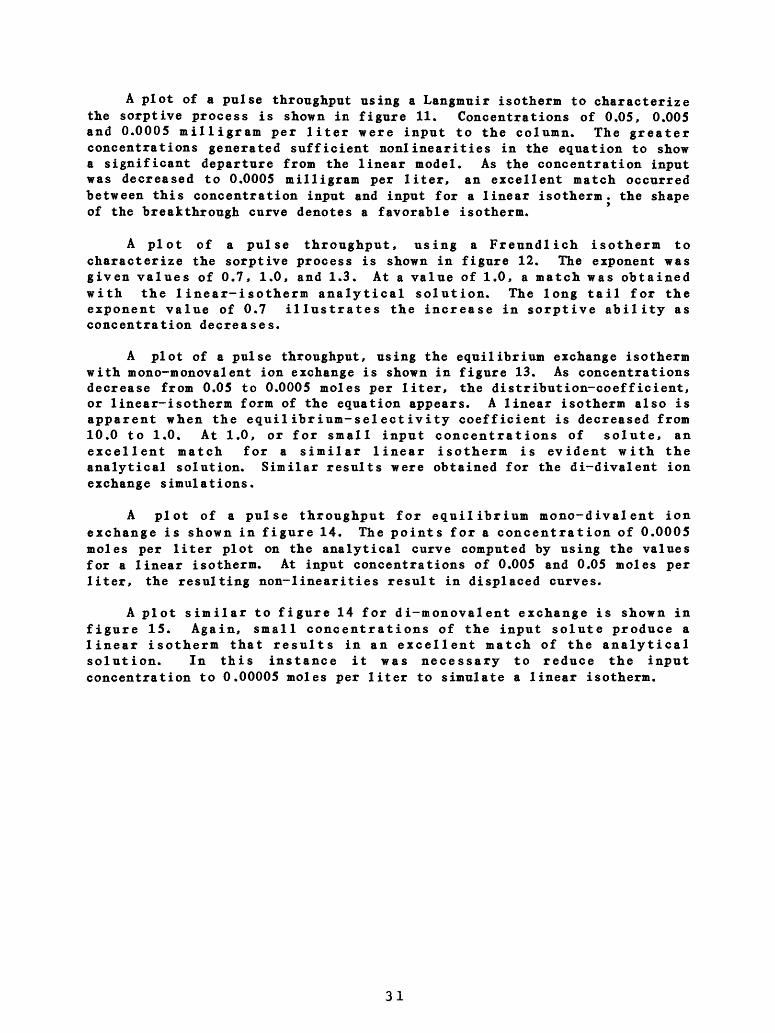
A plot of a pulse throughput using a Langmuir isotherm to characterize the sorptive process is shown in figure 11. Concentrations of 0.05, 0.005 and 0.0005 milligram per liter were input to the column. The greater concentrations generated sufficient nonlinearities in the equation to show a significant departure from the linear model. As the concentration input was decreased to 0.0005 milligram per liter, an excellent match occurred between this concentration input and input for a linear isotherm, the shape of the breakthrough curve denotes a favorable isotherm.

A plot of a pulse throughput, using a Freundlich isotherm to characterize the sorptive process is shown in figure 12. The exponent was given values of 0.7, 1.0, and 1.3. At a value of 1.0, a match was obtained with the linear-isotherm analytical solution. The long tail for the exponent value of 0.7 illustrates the increase in sorptive ability as concentration decreases.

A plot of a pulse throughput, using the equilibrium exchange isotherm with mono-monovalent ion exchange is shown in figure 13. As concentrations decrease from 0.05 to 0.0005 moles per liter, the distribution-coefficient, or linear-isotherm form of the equation appears. A linear isotherm also is apparent when the equilibrium-selectivity coefficient is decreased from 10.0 to 1.0. At 1.0, or for small input concentrations of solute, an excellent match for a similar linear isotherm is evident with the analytical solution. Similar results were obtained for the di-divalent ion exchange simulations.

A plot of a pulse throughput for equilibrium mono-divalent ion exchange is shown in figure 14. The points for a concentration of 0.0005 moles per liter plot on the analytical curve computed by using the values for a linear isotherm. At input concentrations of 0.005 and 0.05 moles per liter, the resulting non-linearities result in displaced curves.

A plot similar to figure 14 for di-monovalent exchange is shown in figure 15. Again, small concentrations of the input solute produce a linear isotherm that results in an excellent match of the analytical solution. In this instance it was necessary to reduce the input concentration to 0.00005 moles per liter to simulate a linear isotherm.

31


OQ0n

o o HH I-* »

pi »d^ rt- &*PS H-HOWH- p ts* o oPS H> ^ W O H*

H fJS g"

"

">

Hp, f 89* S 8. H> P O>o w»P B 88. pj p

H- po

££


Tj H«

000 H

H> CA QO O H H I-* p

p H.H OH. po "pi tA H>

O OQej O« I- P

w S9 oo P oM> g <+

flOQ CA

8?S ^

H- H* 3O rt- o

M H

I p H. t»OP

CA rt-O H.H O

00

CD

CO

X

n > z33 Z Cm > 2!< S3?2 o

m c/)0)o

3E § 35 i

i

i

i

/f 1

H -^

1 1 1 1 1 1 1 1


00aH

< H V)P <D oH *C$ H1 M- H js O 2 rt-

H- O

51

<D

S* O<D V> ^

O 00 H

SB

as s o t» H- OH. o a sP i S *o*3 3 p to

8- § 2.« S ?S OM "^ O

** W MP |-t Q P

O <D ::<D M 3 O

H58 ^**

£§

OQ

m

?c^ m


flH- 000H

2 2 2 ® POOn

H. H d >S

(n O O IA

d o pM VJ *»

o tto B o *^ § d* ° H. o 8 §

» H «'

8 «§ i p a " « 2. f ^ ^T ^^ -kCD T3 O

O M t»-» O

o p H> p pO h->H «1

9


H-

ere

H V) Qffi O H

>d H- Se

ffi S fw H* tn<6 O M

<* f C«to H Ol-« O S*<D S3 _P OQ Of+ >3*

O £ * £, M f)

SB Cfl ^» O

OQ H 2(fc ^^ M

rt- H-H» H- V-j

O O rt-H t> H«

O58

13oJ) m<Oi csm

REFERENCES CITED

Bear, J., 1972, Dynamics of fluids in porous media: New York, American Elsevier, 764 p.

Brenner, H., 1962, The diffusion model of longitudinal mixing in beds of finite length, numerical values: Chemical Engineering Science, v. 17, p. 229-243.

Dankwerts, P. V., 1953, Continuous flow systems: Chemical Engineering Science, v. 2, no. 1, p. 1-13.

Freeze, R. A., and Cherry, J. A., 1979, Groundwater: Englewood Cliffs, N.J., Prentice-Hall, 604 p.

Grove, D. B., 1977, The use of Galerkin finite-element methods to solve mass-transport equations: U.S. Geological Survey Water-Resources Investigations 77-49, 55 p.

Grove, D. B., and Rubin, J., 1977, Transport and reaction of contaminants in ground-water systems: Proceedings of National Conference on Disposal of Residues on Land, St. Louis, Mo., Sept. 13-15, 1976, p. 174-178.

Helfferich, F., 1960, Ion exchange: New York, McGraw-Hill, 624 p.

Levenspiel, 0., 1972, Chemical reaction engineering: New York, John Wiley & Sons, 578 p.

Vermeulen, T., 1973, Adsorption and ion exchange in Chemical Engineers Handbook-Fifth Edition, chapter 16: New York, McGraw Hill, 1944 p.

Von Rosenberg, D. V., 1969, Methods for the numerical solution of partial differential equations: New York, American Elsevier, 128 p.

37

SUPPLEMENTAL DATA

38

Attachment I.

Definition of Selected Program Variables

A(I) Solution-matrix coefficient.

ACC Solute accumulated in column

ALPHA Hydraulic-dispersion characteristic length.

B(I) Solution-matrix coefficient.

C(I) Solution-matrix coefficient.

CDELT Fraction of cell distance that ion moves.

CDIM Dimensionless concentration.

CEC Cation-exchange capacity.

CI Initial concentration entering reactor.

COEF(I) Array that stores (1+RHOB*SLOPE/POR).

CON(I) Solute concentration at node I.

CTOT Total-solution concentration.

D(I) Solution- matrix coefficient (known values).

DELT Time increment.

DIP Molecular-diffusion coefficient times torosity.

DIM Dimensionless concentration (CON/CI).

DIS Dispersion coefficient.

DPUL Time of pulse input.

DT DELT/COEF.

DX Distance increment.

EK Ion-exchange equilibrium constant.

EKF Freundlich-isotherm constant.

EEL Langmuir-isotherm constant.

FCTF Variable for Freundlich isotherm.

FCTL Variable for Langmuir isotherm.

39

FCTM Variable for exchange isotherm.

FRAC Fraction of input-exiting column.

HEAD Heading to be printed out.

1C GT 0 for constant concentration boundary condition,

INPUT Name of data input file.

K Chemical-reaction rate constant.

N Number of time steps.

NEXC Sets type of sorption process (0-6).

NI Number of nodes in column.

NJ Node number of printout.

NK Number of nodes for parameter calculations.

NLIN 1 for linear isotherm.

NNI Suggested number of nodes to prevent oscillation.

NP1 GT 0 to print last node only.

NP2 Increment of node printout.

NP3 Set equal to 7 for plotting output.

OUTPUT Name of output file.

PE Dimensionless-dispersion variable (VAXL/DIS)

PFILE Name of plot file.

PIPV Pore-volume increment between printouts.

PON(I) Intermediate values of concentration at DELT/2.

FOR Effective porosity.

PPV Incremental pore-volume output.

PSTOP Number of pore volumes in run.

RCOE(I) Array that stores (1+RHOB*SLOPE/FOR).

RHOB Soil-bulk density.

RX(I) Array that stores rate variable (K*CON*RCOE/2).

40

CBAR(I) Concentration on the solid phase.

SCC Solute sorbed in column.

STA Oscillation coefficient.

TIME Total time of column run.

TKOUT Solute output by chemical reaction.

TTIME Incremental time between printouts.

V Interstitial-fluid velocity.

XDIM Dimensionless-column length.

XDIM(I) Dimensionless distance.

XIN Solute input to the column.

XE Dimensionless rate variable (K*XL/V)

XL Column length.

XMB Fractional mass balance error.

XNF Slope of Freundlich isotherm.

XODT Solute output from the column.

41

Attachment II.

Data-Input Formats

Line

1

Data number Variable

1 HEAD

1 NEXC

3

4

5

8

9

10

11

12

1C

NI

DELT

PSTOP

PIPV

NP1

NP2

NP3

NJ

CDELT

NK

Definition

Description of problem (as many as 70 characters).

Type of sorption; 0 = none, 1 = Freundlich, 2 = Langmuir,3 = mono-monovalent,4 =di-divalent5 = mono-divalent,6 = Di-monovalent.

Greater than 0 for constant - concentration boundary condition

Number of nodes.

Time increment.

Number of pore volumes in simulation

Pore-volume increment between printout.

Greater than 0 to print concentration at node number NJ.

Increment of node printout.

Set equal to 7 to write output to disk for plotting.

Node number for data printout.

Fraction of cell distance a solute will move, if greater than 0, computes a new DELT.

Number of nodes for parameter calculation.

42

3

3

3

3

3

3

3

4

4

4

4

4

4

4

4

1

2

3

4

5

6

7

1

2

3

4

5

6

7

8

DPUL

XL

V

DIP

ALPHA

RHOB

FOR

SLOPE

CI

CEC

CTOT

K

EKF

XNF

EK

EEL

Time of pulse input.

Column length.

Fluid velocity.

Molecular-diffusion constant.

Hydraulic-dispersion charac teristic length.

Soil-bulk density.

Effective porosity.

Linear-isotherm slope.

Input-solute concentration.

Total sorption capacity of soil.

Total solution concentration.

First-order rate constant.

Freundlich-isotherm constant.

Slope of Freundlich isotherm,

Exchange-equilibrium coefficient.

Langmuir isotherm constant.

43

Attachment III.

Input Data for Selected Figures

Record Line Free Field Data Input

1 PULSE WITH NO CHEMICAL REACTIONS - FIGURE 9

2 0, 1, 101, .2, 3, .1, 1, 1, 7, 51, .2, 51

3 80, 16, .1, 0, 1, 1.587, .37

4 0, .05, 0, 0, 0, 0, 0, 0, 0

Comments

Output from the column is at node 51 for all parameters such as pore volume, Brenner number, and so forth. This is to allow a comparison with an analytical solution that has the assumption of an infinite column. Pore volume and relative concentration data was printed out for a computer plot.

1. LINEAR SORPTION AND KINETICS - FIGURE 10 -

2. 0, 1, 101, .2, 6, .2, 1, 1, 7, 51, .2, 51

3. 160, 16, .1, 0, 1, 1.587, .37

4. .3, .05, 0, 0, .01, 0, 0, 0, 0

Comments

As in the previous example, a value of 0.2 for CDELT results in the input value of DELT being overridden. A new value of DELT is then computed by the subprogram NEWDT to be 0.73.

1. NON-LINEAR LANGMUIR SORPTION - FIGURE 11

2. 2, 1, 101, .2, 6, .2, 1, 1, 7, 51, 0, 51

3. 160, 16, .1, 0, 1, 1.587, .37

4. 0, .05, .003, 0, 0, 0, 0, 0, 100

Comments

A Langmuir isotherm is assumed with most of the other values the same. The value of DELT of 0.2 was not overridden this time. Values for CEC of 0.003 and EEL of 100. were chosen for comparison with the linear isotherm slopes of 0.3.

44

1. NON-LINEAR FREUNDLICH SORPTION - FIGURE 12

2. 1, 1, 101, .2, 6, .2, 1, 1, 7, 51, .2, 51

3. 160, 16, .1, 0, 1, 1.587, .37

4. 0, .05, 0, 0, 0, .3, .7, 0, 0

Comments

A Freundlich isotherm is assumed with an exponent of 0.7. As shown in figure 12, a sharp peak with a long tail results.

1. DI-DIVALENT ION EXCHANGE

2. 4, 1, 101, .5, 6, .4, 1, 1, 7, 51, .2, 51

3. 160, 16, .1, 0, 1, 1.587, .37

4. 0, .05, .003, .1, 0, 0, 0, 10, 0

Comments

Di-divalent ion exchange is assumed. Output for this example is shown as attachment IV.

45

Attachment IV.

Example of computer output

* ** DI-DIVALENT ION EXCHANGE ** *

0 USER DEFINED OPTIONS AND PARAMETERS

0 TIME INCREMENT(DELT)............................. 0.5000PORE VOLUME INCREMENT BETWEEN PRINTOUTS(PIPV).... 0.4000NUMBER OF NODES(NI).............................. 101TOTAL PORE VOLUME OF RUN(PSTOP).................. 6.0000PRINT NODE NJ ONLY(NP1)..........................YESNODE FOR PRINTOUT(NJ)............................ 51NUMBER OF NODES FOR PARAMETER CALCULATION(NK).... 51INCREMENT OF NODE PRINTOUT(NP2).................. 1NAME OF PLOT DATA FILE(PFILE)....................RPT14.PLTFLUX INPUT BOUNDRY CONDITION(1C).................NOFRACTION OF CELL THAT ION MOVES(CDELT)...........0.20CODE FOR POSSIBLE SORPTION(NEXC).................EXCHANGE(4)

PHYSICAL CHARACTERISTICS OF COLUMN,SOIL, AND SOLUTE

TIME DURATION"OF PULSE(DPUL)..................... 0.160E+03COLUMN LENGTH(XL)................................ 16.000INTERSTITIAL FLUID VELOCITY(V)................... 0.100E+00MOLECULAR DIFFUSION COEF(DIF).................... 0.OOOE+00DISPERSION CHARACTERISTIC LENGTH(ALPHA).......... 1.000MEDIUM BULK DENSITY(RHOB)........................ 1.587MEDIUM POROSITY(POR)............................. 0. 370

CHEMICAL CHARACTERISTICS OF POROUS MEDIUM AND SOLUTE

SLOPE OF LINEAR ISOTHERM(SLOPE).................. O.OOOE+00SOLUTE INPUT CONCENTRATIONCI)................... 0.500E-01SORPTION OR CATION EXCHANGE CAPACITY(CEC)........ 0.003TOTAL SOLUTION CONCENTRATIONCTOT)............... 0.100E+00KINETIC RATE CONSTANT(K)......................... O.OOOE+00FREUNDLICH ISOTHERM CONSTANT(EKF)................ O.OOOE+00EXPONENT OF FREUNDLICH ISOTHERM(XNF)............. 0.000ION EXCHANGE CONSTANT(EK)........................ 0.100E+02LANGMUIR SORPTION CONSTANT(EKL).................. O.OOOE+00

46

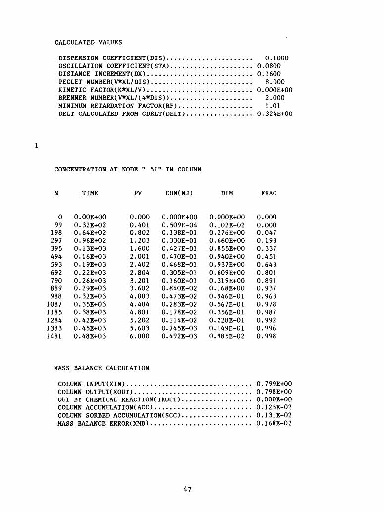
CALCULATED VALUES

DISPERSION COEFFICIENT(DIS).....OSCILLATION COEFFICIENTSTA)....DISTANCE INCREMENT(DX)..........PECLET NUMBER(V*XL/DIS).........KINETIC FACTOR(K*XL/V)..........BRENNER NUMBER(V*XL/(4*DIS))....MINIMUM RETARDATION FACTOR(RF).. DELT CALCULATED FROM CDELT(DELT)

0.1000 0.0800 0.1600

8.000 O.OOOE-l-00

2.0001.01

0.324E+00

CONCENTRATION AT NODE " 51" IN COLUMN

N TIME PV CON(NJ) DIM FRAC

099

198297395494593692790889988

10871185128413831481

O.OOE-i-00 0.32E+02 0.64E+02 0.96E-I-02 0.13E+03 0.16E+03 0.19E+03 0.22E+03 0.26E+03 0.29E+03 0.32E+03 0.35E+03 0.38E+03 0.42E+03 0.45E+03 0.48E+03

0.0000.4010.8021.2031.6002.0012.4022.8043.2013.6024.0034.4044.8015.2025.6036.000

O.OOOE+000.509E-040.138E-010.330E-010.427E-010.470E-010.468E-010.305E-010.160E-010.840E-020.473E-020.283E-020.178E-020.114E-020.745E-030.492E-03

O.OOOE+000.102E-020.276E+000.660E+000.855E-I-000.940E+000.937E+000.609E+000.319E+000.168E+000.946E-010.567E-010.356E-010.228E-010.149E-010.985E-02

0.0000.0000.0470.1930.3370.4510.6430.8010.8910.9370.9630.9780.9870.9920.9960.998

MASS BALANCE CALCULATION

COLUMN INPUT(XIN)..............COLUMN OUTPUT(XOUT)............OUT BY CHEMICAL REACTION(TKOUT) COLUMN ACCUMULATION(ACC).......COLUMN SORBED ACCUMULATION. SCC) MASS BALANCE ERROR(XMB)........

0.799E+00 0.798E+00 O.OOOE+00 0.125E-02 0.131E-02 0.168E-02

47

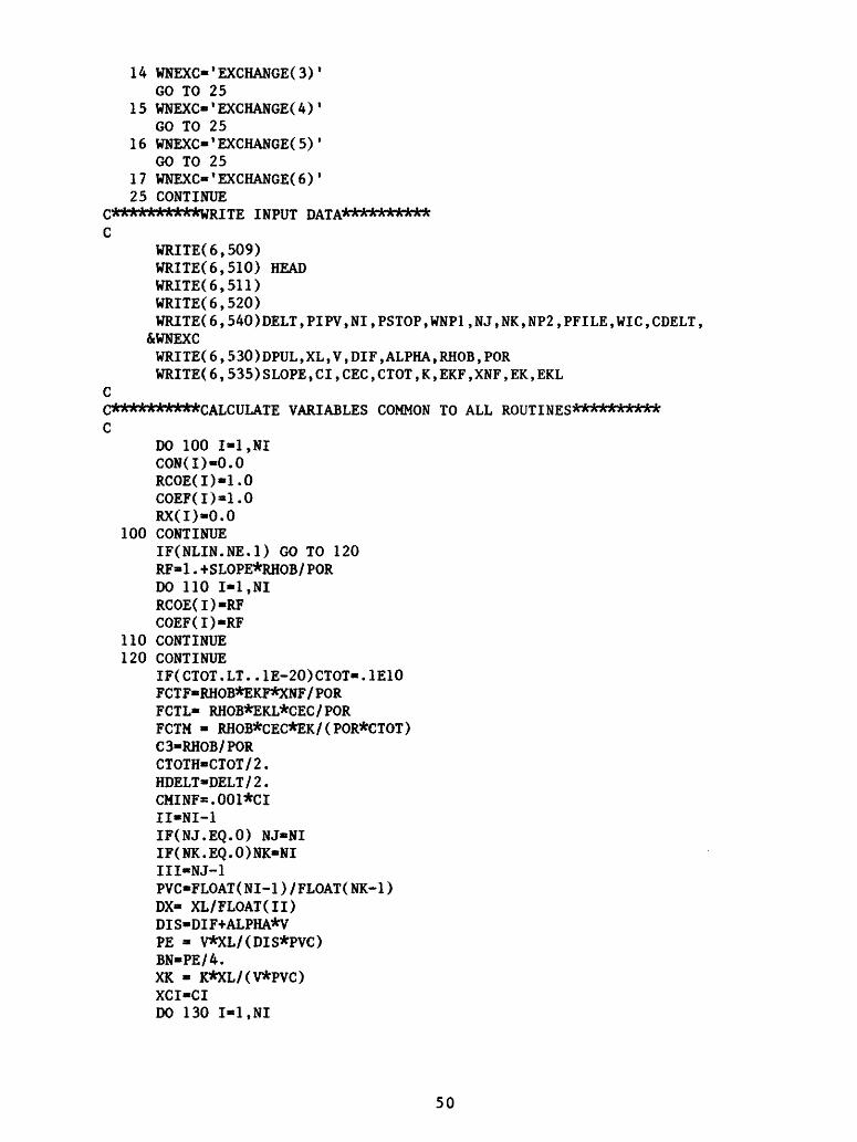
Attachment V.

FORTRAN 77 program listing *^**»***j|^C**^bbM-ifrJtt-A^^ C^ffHriblf***^^C THIS PROGRAM CALCULATES THE CONCENTRATION PROFILE EXITING FROMC OR WITHIN A SOIL COLUMN AS A FUNCTION OF TIME.C THE PROGRAM UTILIZES A CRANK-NICOLSON FINITE DIFFERENCEC APPROXIMATION TO THE DEFINING DIFFERENTIAL EQUATION AND THEC DOUGLAS PREDICTOR-CORRECTOR METHOD TO ACCOUNT FOR THEC POSSIBLE NON-LINEAR SORPTION TERM.C EQUILIBRIUM CONTROLLED SORPTION IS ACCOUNTED FOR BYC EITHER THE MASS ACTION LAW, THE LANGMIUR, OR -FREUNDLICH ISOTHERMC A FIRST ORDER IRREVERSIBLE RATE REACTION IS INCLUDED.C PROGRAM WRITTEN BY D. GROVE,U.S.GEOLOGICAL SURVEYC WATER RESOURCES DIVISION, DENVER COLORADO, NATIONALC RESEARCH PROGRAM ON 6/83.C***abHMbM^C^Hf**^frA-ArfrA^^C ALPHA - HYDRAULIC DISPERSION CHARACTERISTIC LENGTHC CDELT - FRACTION CELL DISTANCE A SOLUTE WILL MOVE IN DELTC CEC - CATION EXCHANGE CAPACITYC CI - INITIAL CONCENTRATION ENTERING REACTORC CTOT » TOTAL SOLUTION CONCENTRATIONC DELT * TIME INCREMENTC DIF - MOLECULAR DIFFUSION COEFFICIENTC DPUL * TIME OF PULSE INPUTC EK » ION EXCHANGE EQUILIBRIUM CONSTANTC EKF - FREUNDLICH ISOTHERM CONSTANTC EKL * LANGMIUR ISOTHERM CONSTANTC 1C * GT 0 FOR CONSTANT CONCENTRATION BOUNDRY CONDITIONC K * CHEMICAL REACTION RATE CONSTANTC NEXC * 0 FOR NO ADSORPTIONC - 1 FOR FREUNDLICH ISOTHERMC - 2 FOR LANGMUIR ISOTHERMC - 3 FOR MONO-MONO EXCHANGEC * 4 FOR DI-DIVALENT EXCHANGEC - 5 FOR MASS ACTION EXCHANGE WITH 2M+«2MXC - 6 FOR MASS ACTION EXCHANGE WITH M-H MX2C NI - NUMBER OF NODES IN COLUMNC NK - NUMBER OF NODES FOR PARAMETER CALCULATIONC NJ * NODE NUMBER OF DATA PRINTOUTC NP1 - GT 0 TO PRINT NODE NJ ONLYC NP2 - INCREMENT OF NODE PRINTOUTC NP3 - 7 FOR DISK OUTPUT FOR PLOT ROUTINESC PIPV - PORE VOLUME INCREMENT BETWEEN PRINTOUTSC POR - EFFECTIVE POROSITYC PSTOP - NUMBER OF PORE VOLUMES AT NJ IN REACTOR RUNC RHOB - SOIL BULK DENSITYC SLOPE - LINEAR SLOPE OF SORPTION ISOTHERMC V - INTERSTITIAL FLUID VELOCITYC XL - COLUMN LENGTH AT NIC XNF - SLOPE OF FREUNDLICH ISOTHERMC*IMMblMMb(^^

48

DIMENSION A(201),B(201),C(201),D(201),CON(201),CE(201),X(201), &PON(201),RX(201),S(201),COEF(201),RCOE(201)REAL KCHARACTER HEAD*80 , INPUT*10 , OUTPUT*10 , PFILE*! 2 , Fl*10 , 1WNP1*3,WNP3*3,WIC*3,WNEXC*12

CC**********INITIALIZE VARIABLES********** C

TKOUT-0.0WNPl-'NO 1PFILE- 'NO PLOT FILE 1WIC-'NO'F1*'(A)'

ACC«0.0RF-1.0N6«0N «0FRAC-0.0TIME-0.0NLIN -0XIN » 0.0XOUT-0.0PPV«0 . 0PV«0.0

INPUT DATA********'***************

WRITE (*,F1)'TYPE IN NAME OF INPUT FILE' READ (*,F1) INPUTWRITE (*,F1)'TYPE IN NAME OF OUTPUT FILE' READ (*,F1) OUTPUT OPEN(5,FILE«INPUT) OPEN( 6, FILE-OUTPUT) READ (5,F1) HEADREAD(5,*)NEXC,IC,NI,DELT,PSTOP,PIPV,NP1,NP2,NP3,NJ,CDELT,NK READ(5,*)DPUL,XL,V,DIF,ALPHA,RHOB,POR READ( 5 , * ) SLOPE , CI , CEC , CTOT , K , EKF , XNF , EK , EKL IF(NPl.GT.O) WNPl-'YES' IF(IC.EQ.O) WIC«'YES' IF(ABS( SLOPE). GT..1E-20)NLIN*1 IF(NP3.NE.7) GO TO 50WRITE (*,F1)'TYPE IN NAME OF PLOT FILE' READ(*,F1) PFILE OPEN(7,FILE«PFILE)

50 CONTINUE

NGO-NEXC+1GO TO(11,12,13,H,15,16,17),NGO

11 WNEXC«'NONE* GO TO 25

12 WNEXC-'FREUNDLICH* GO TO 25

13 WNEXC«'LANGMUIR' GO TO 25

49

14 WNEXO'EXCHANGEO) 1 GO TO 25

15 WNEXO 1 EXCHANGE(4)' GO TO 25

16 WNEXO'EXCHANGE(5)' GO TO 25

17 WNEXO 1 EXCHANGE(6)' 25 CONTINUE

C**********WRIXE INPUT DATA********** C

WRITE(6,509)WRITE(6,510) HEADWRITE(6,511)WRITE(6,520)WRITE(6,540)DELT,PIPV,NI,PSTOP,WNP1,NJ,NK,NP2,PFILE,WIC,CDELT,

&WNEXCWRITE(6,530)DPUL,XL,V,DIF,ALPHA,RHOB,PORWRITE(6,535)SLOPE,CI,CEC,CTOT,K,EKF,XNF,EK,EKL

CC**********CALCULATE VARIABLES COMMON TO ALL ROUTINES********** C

DO 100 1*1,NICON(I)«0.0RCOE(I)«1.0COEP(I)«1.0RX(I)*0.0

100 CONTINUEIF(NLIN.NE.l) GO TO 120RF-1.+SLOPE*RHOB/PORDO 110 I-l.NIRCOE(I)-RFCOEF(I)«RF

110 CONTINUE 120 CONTINUE

IF(CTOT.LT..1E-20)CTOT«.1E10FCTF«RHOB*EKF*XNF/PORFCTL« RHOB*EKL*CEC/PORFCTM « RHOB*CEC*EK/(POR*CTOT)C3«RHOB/PORCTOTH-CTOT/2.HDELT-DELT/2.CMINF*.001*CIII-NI-1IF(NJ.EQ.O) NJ«NI IF(NK.EQ.O)NK«NIIII-NJ-1PVC«FLOAT(NI-1)/FLOAT(NK-1)DX« XL/FLOAT(II)DIS-DIF-I-ALPHA*VPE » V*XL/(DIS*PVC)BN-PE/4.XK « K*XL/(V*PVC)XCI-CIDO 130 1*1,NI

50

130 X(I)»DX*(FLOAT(I)-1.)IF(CDELT.LT.. IE-20) GO TO 140CALL NEWDT( NLIN , CDELT , DX , V , NGO , FCTF , FCTL , FCTM , XNF , CI , EKL , CTOT , EK ,

&CEC , RHOB , POR , RF , DELT ) 140 CONTINUE

D2*DIS/(DX*DX)D4» V/(4.*DX) + DIS/(2.*DX*DX)D6 - -V/(4.*DX) + DIS/(2.*DX*DX)D7 » DIS/(DX*DX)I«lA(I)»0.0C(I)« -DIS/(DX*DX)IF(IC.GT.O) C(l)«0.0DO 150 I«2,II

-V/(4.*DX) - DIS/(2.*DX*DX) V/(4.*DX) - DIS/(2.*DX*DX)

150 CONTINUE

-DIS/(DX*DX)C(I)«0.0

CC*****THE VARIABLE STA MUST BE EQUAL TO OR LESS THAN ONE TO PREVENT C*****UNDAMPED OSCILLATION FROM OCCURING DURING SOLUTION. C

STA * V*DX/(2.*DIS)IF(STA.LT.l.O) GO TO 160WRITE(6,560) STANNI- XL*V/(2.*DIS)+2.WRITE(6,470) NNISTOP

160 CONTINUE CC**********WRIXE CALCULATED DATA********** C

WRITE(6,536) DIS, STA, DX,PE,XK,BN,RF, DELT 170 CONTINUE

IF(PV.LT.(PPV-.0001» GO TO 220PPV * PPV + PIPVIF(NPl.LT.l) GO TO 200IF(N6.GT.O) GO TO 180WRITE(6,460) NJN6«l

180 CONTINUEIF(XIN.LT.0.1E-20)GO TO 190FRAC«XOUT/XIN

190 CONTINUECDIM-CON(NJ)/XCIWRITE(6,450) N, TIME, PV, CON( NJ) , CDIM, FRACIF(NP3.EQ.7)WRITE(NP3,440)PV,CDIMGO TO 220

200 CONTINUEWRITE(6,580) TIME,N,PVDO 210 I«1,NJ,NP2CDIM»CON(I)/XCI

51

XDIM-X(I)/XLWRITE(6,570) I,X(I),XDIM,CON(I),CDIMIF(NP3.EQ.7)WRITE(7,440) XDIM,CDIM


IF(PV.GT.PSTOP) GO TO 420IF(NLIN.EQ.l) GO TO 280GO T0(280,230,240,250,255,260,270),NGO

CC********^CALCULATE THE ISOTHERM COEFFICENTS********** C

230 CALL FREUN(CON,CMINF,RCOE,FCTF,XNF,COEF,NI)GO TO 280

240 CALL LANG(NI,RCOE,FCTL,EKL,CON,COEF)GO TO 280

250 CALL EXC(NI,RCOE,FCTM,CTOT,CON,EK,COEF)GO TO 280

255 CALL EXC(NI,RCOE,FCTM,CTOTH,CON,EK,COEF)GO TO 280

260 CALL EXCM(NI,CON,CMINF,CTOT,EK,CEC,RCOE,COEF,C3)GO TO 280

270 CALL EXCD(NI,EK,CEC,CTOT,CON,CMINF,C3,RCOE,COEF) 280 CONTINUE

IF(K.LT..IE-20) GO TO 300DO 290 1*1,NIRX(I)«K/2.*RCOE(I)


IF(NEXC.EQ.O.OR.NLIN.EQ.l) GO TO 380 CC*teHr******CALCULATE CONCENTRATION AT TIME DELT/2********** C

CALL REACT(HDELT,COEF,DIS,DX,V,RX,CON,D1,D2,IC,CI,II,NI,D4,D5,D6, &D7,A,B,C,D,PON)

CC**********cALCULATE ISOTHERM COEFFICIENTS AT TIME+DELT/2**** C

GO 10(360,310,320,330,335,340,350),NGO 310 CALL FREUN(PON,CMINF,RCOE,FCTF,XNF,COEF,NI)

GO TO 360 320 CALL LANG(NI,RCOE,FCTL,EKL,PON,COEF)

GO TO 360 330 CALL EXC(NI,RCOE,FCTM,CTOT,PON,EK,COEF)

GO TO 360 335 CALL EXC(NI,RCOE,FCTM,CTOTH,PON,EK,COEF)

GO TO 360 340 CALL EXCM(NI,PON,CMINF,CTOT,EK,CEC,RCOE,COEF,C3)

GO TO 360350 CALL EXCD(NI,EK,CEC,CTOT,PON,CMINF,C3,RCOE,COEF) 360 CONTINUE

IF(K.LT..IE-20) GO TO 380DO 370 I-l.NIRX(I)-K/2.*RCOE(I)

370 CONTINUE

52

380 CONTINUE CC**********CALCULATE CONCENTRATION AT TIME + DT********** C

CALL REACT(DELT,COEF,DIS,DX,V,RX,CON,D1,D2,IC,CI,II,NI,D4,D5,D6, &D7,A,B,C,D,CON)

390 CONTINUETIME * TIME + DELT IF(DPUL.LT..IE-20) GO TO 400IF(TIME.GT.DPUL)CI»0.0

400 CONTINUEIF(K.LT..IE-20) GO TO 407 XKOUT*CON(1)*RCOE(1)/2. DO 405 I»2,III

405 XKOUT«XKOUT+CON(I)*RCOE(I)XKOUT»XKOUT+CON(NJ)*RCOE(NJ)/2. XKOUT«XKOUT*K*DELT*DX TKOUT-TKOUT+XKOUT

407 CONTINUEPV*PVC*V*TIME/XL XIN»CI*V*DELT+XIN XOUT*XOUT+CON( NJ)*V*DELT N»N+1 GO TO 170


CC**********CALCULATE MASS BALANCE********** C

SCC«CON(1)*(RCOE(1)-l.)/2. DO 430 I«2,III SCC-SCC4-CON( I) *( RCOE( I) -1.)

430 ACC»ACC+CON(I)ACC*ACC*DX+(CON(1)+CON(NI))*DX/2. SCC»(SCC+CON(NJ)*(RCOE(NJ)-1.)/2.)*DX XMB*(ACC+SCC+XOUT+TKOUT-XIN)/XIN WRITE(6,600) XIN,XOUT,TKOUT,ACC,SCC,XMB

CC*^*r*******FORMAT STATEMENTS********** C

440 FORMAT(F11.3,E12.3)450 FORMAT(1H ,IX,15,Ell.2.F11.3,2E12.3,F8.3,E12.3)460 FORMAT(1HI,///,5X, f CONCENTRATION AT NODE " f ,I3,' lf IN COLUMN 1 ,///

&,5X,'N '5X,'TIME 1 ,9X,'PV',6X,'CON(NJ)',7X,'DIM 1 , &7X, f FRAC f //)

470 FORMAT(1HO, 'OSCILLATION CAN BE ELIMINATED BY INCREASING THE 1 ,/ &'NUMBER OF NODES (NI) TO f ,I5)

509 FORMAT(1H , **HMlRlttlf**JM^^ « 9 &»*jlrilriHlf^"A^^^ ' / IX, '*' ,T78, '*')

510 FORMATdH ,'*', 3X,A,T78,'*')511 FORMAT(1H ,'*',T78, t *'/lX,' »ATlttlrilrilrA"A^^^ ' ,

&' ilnlMlr»JMMMinln^^ ' / / ) 520 FORMATUHO,' USER DEFINED OPTIONS AND PARAMETERS',//) 540 FORMATUHO,

53

&5X,'TIME INCREMENT(DELT)............................. f ,F7.4/&6X,'PORE VOLUME INCREMENT BETWEEN PRINTOUTS(PIPV)....',F9.4/&6X,'NUMBER OF NODES(NI).............................. f ,I3/&6X,'TOTAL PORE VOLUME OF RUN(PSTOP).................. l ,F9.4/&6X,'PRINT NODE NJ ONLY(NP1)..........................',A/&6X,'NODE FOR PRINTOUT(NJ)..........................., l ,I3/&6X,'NUMBER OF NODES FOR PARAMETER CALCULATION(NK)....',I3/&6X,'INCREMENT OF NODE PRINTOUT(NP2)..................',I3/&6X,'NAME OF PLOT DATA FILE(PFILE)....................',A/&6X,'FLUX INPUT BOUNDRY CONDITION(IC).................',A/&6X,'FRACTION OF CELL THAT ION MOVES(CDELT)...........',F4.2/&6X,'CODE FOR POSSIBLE SORPTION(NEXC)................, l ,A)

530 FORMAT(1H ,///,5X,'PHYSICAL CHARACTERISTICS OF COLUMN,SOIL,' &' AND SOLUTE 1 ,//, &6X,'TIME DURATION OF PULSE(DPUL).....................',E10.3/&6X,'COLUMN LENGTH(XL)................................ l ,F8.3/&6X,'INTERSTITIAL FLUID VELOCITY(V)................... f ,E10.3/&6X,'MOLECULAR DIFFUSION COEF(DIF)....................',E10.3/&6X,'DISPERSION CHARACTERISTIC LENGTH(ALPHA)..........',F9.3/&6X,'MEDIUM BULK DENSITY(RHOB)........................',F8.3/&6X,'MEDIUM POROSITY(POR)............................. f ,F8. 3)

535 FORMAT(1H ,///,5X,'CHEMICAL CHARACTERISTICS OF POROUS', &' MEDIUM AND SOLUTE',//, &6X,'SLOPE OF LINEAR ISOTHERM(SLOPE)..................',E10.3/&6X,'SOLUTE INPUT CONCENTRATIONCI)...................',E10.3/&6X,'SORPTION OR CATION EXCHANGE CAPACITY(CEC)........',F9.3/&6X,'TOTAL SOLUTION CONCENTRATION(CTOT)...............',E10.3/&6X,'KINETIC RATE CONSTANT(K).........................',E10.3/&6X,'FREUNDLICH ISOTHERM CONSTANT(EKF)................',E10.3/&6X,'EXPONENT OF FREUNDLICH ISOTHERM(XNF).............',F8.3/&6X,'ION EXCHANGE CONSTANT(EK)........................',E10.3/&6X,'LANGMUIR SORPTION CONSTANT(EKL)..................*,E10.3)

560 FORMAT(1H ,'PROGRAM CANCLED BECAUSE STA *',E14.7,',IS', &' GREATER THAN THE MINIMUM VALUE OF ONE')

536 FORMAT(1H ,///,5X,'CALCULATED VALUES',//&6X,'DISPERSION COEFFICIENT(DIS)......................',F9.4/&6X,'OSCILLATION COEFFICIENTSTA)..................... f ,F7.4/&6X,'DISTANCE INCREMENT(DX)...........................',F7.4/&6X,'PECLET NUMBER(V*XL/DIS)..........................',F8.3/&6X,'KINETIC FACTOR(K*XL/V)...........................*,E10.3/&6X,'BRENNER NUMBER(V*XL/(4*DIS)).....................',F8.3/&6X,'MINIMUM RETARDATION FACTOR(RF)...................',F7.2/&6X,'DELT CALCULATED FROM CDELT(DELT).................',E10.3///)

570 FORMAT(1H , 5X,H4,5(3X,E10. 3))580 FORMATdHl, //6X,'CONCENTRATION WITHIN THE COLUMN',//,6X,

&6HTIME «,E9.3,/6X,22HNUMBER OF ITERATIONS *,I7/6X, 24HNUMBER OF PO &RE VOLUMES *,F9.4,//6X,4HNODE,5X, 8HDISTANCE,3X,'DIM DISTANCE', & 4X,'CONC',7X,'DIM CONC')

600 FORMAT(1H ,///5X,'MASS BALANCE CALCULATION 1 ,//&6X,'COLUMN INPUT(XIN)................................',E10.3/&6X,'COLUMN OUTPUT(XOUT)..............................',E10.3/&6X,'OUT BY CHEMICAL REACTION(TKOUT)..................',E10.3/&6X,'COLUMN ACCUMULATIONACC).........................',E10.3/&6X,'COLUMN SORBED ACCUMULATIONSCC)..................',E10.3/&6X,'MASS BALANCE ERROR(XMB)..........................',E10.3)

54

590 FORMAT(E14.7)STOPEND

C CC******n«r***THIS ROUTINE IS THE THOMAS ALGOTHRIUM USED******* C**********TO SOLVE THE TRI -DIAGONAL MATRIX******** C

SUBROUTINE TRIMAT(A,B,C,D,H,II ,NI)DIMENSION A(NI),B(NI),C(NI),D(NI),H(NI),BETA(201),GAMMA(201)I«lBETA(1)»B(1) GAMMA(1)«D(1)/B(1) DO 100 I«2,NIBETA(I)»B(I)-A(I)*C(I-1)/BETA(I-1) GAMMA(I)« (D(I)-A(I)*GAMMA(I-1))/BETA(I)

100 CONTINUEH(NI)« GAMMA(NI) DO 110 J-1,11

H(I)«GAMMA(I)-C(I)*H(I+1)/BETA(I) 110 CONTINUE

RETURNEND

C CC:Hnfc*******THIS SUBROUTINE SOLVES THE QUADRATIC EQUATION**** C

FUNCTION QUADX(A,B,C,D)QUADX»(-B+D*SQRT(B*B-4.*A*C))/<2.*A)RETURNEND

C CC**********THIS SUBROUTINE CALCULATES THE NEW DELT NECESSARY***** C****^nfe****TO MOVE A SORBING SOLUTE CDELT FRACTION OF A CELL DISTANCE** C

SUBROUTINE NEWDT (NLIN, CDELT, DX, V, NGO, FCTF, FCTL, FCTM, XNF, CI ,EKL, &CTOT , EK , CEC , RHOB , FOR , RF , DELT )

CC55-CDELT*DX/VIF(NLIN.EQ.l) GO TO 160GO 10(100,110,120, 130, 135, 140, 150), NGO

100 DELT-C55GO TO 170

110 RF«1.+FCTF*CI**(XNF-1.)DELT«C55*RFGO TO 170

120 RF-1.+FCTL/(1.+EKL*CI)**2DELT-C55*RFGO TO 170

1 30 RF«1 .+FCTM/(CI/CTOT*(EK-1 . )+l . )**2DELT«C55*RFGO TO 170

55

135 RF«1.+FCTM/(2.*CI/CTOT*(EK-1.)+l.)**2DELT « C55*RFGO TO 170

140 C3«RHOB/PORC2«CI*CIAA«CTOT-CIBB»C2*EKCC EK*CEC*C2CBAR-QUADX(AA,BB,CC,1.)DCBAR*(CBAR*CBAR-CBAR*2.*CI*EK+2.*CI*EK*CEC)

&/((CTOT-CI)*2.*CBAR+C2*EK)RF*1.+C3*DCBARDELT*C55*RFGO TO 170

150 C4-EK*CECC3-RHOB/PORC5«C4*CECC6»CTOT*CTOTC2»CI*CIAA»EK*CI*4.BB*-4.*C4*CI-C6+4.*CI*CTOT-4.*C2CC»C5*CICBAR«QUADX(AA,BB,CC,-1.)DCBAR»(-4.*CBAR*CBAR*EK-CBAR*(-4.*C4+4.*CTOT-8,*CI)

&-C5)/(4.*EK*CI*(2.*CBAR-CEC)-C6+4.*CI*CTOT-C2*4.)RF»1.+C3*DCBARDELT-C55*RFGO TO 170

160 DELT»C55*RF 170 CONTINUE

RETURNEND

C CC**********THIS SUBROUTINE COMPUTES THE COEFFICIENTS******** C**********FOR THE LANGMUIR SORPTION****************^^^ C

SUBROUTINE LANG(NI,RCOE,FCTL,EKL,CON,COEF)DIMENSION RCOE(NI),CON(NI),COEF(NI)DO 100 I-l.NIRCOE(I)»1.+FCTL/(1.+EKL*CON(I))

100 COEF(I)«1.+FCTL/((1.+EKL*CON(I))**2)RETURNEND

C CC**nMr******THIS SUBROUTINE COMPUTES THE COEFFICIENTS****1***1**' C**********FQR EQUAL VALENCE ION EXCHMGE**"*1**"********* C

SUBROUTINE EXC(NI,RCOE,FCTM,CTOT,CON,EK,COEF)DIMENSION RCOE(NI),CON(NI),COEF(NI)DO 100 I-l.NIRCOE(I)»1.+FCTM*CTOT/((CTOT-CON(I))+EK*CON(I))

100 COEF(I) « l.+FCTM/((CON(I)/CTOT*(EK-l.)+l.)**2)RETURNEND

56

c cC**********THIS SUBROUTINE COMPUTES THE COEFFICIENTS*******C**********FOR MONO-VALENT DIVALENT*****"*****"*"**^^C

SUBROUTINE EXCM(NI ,CON,CMINF,CTOT,EK,CEC,RCOE,COEF,C3)DIMENSION RCOE( NI ) , CON( NI ) , COEF( NI )DO 110 1*1, NIIF(CON(I).LT.CMINF) GO TO 100C2*CON(I)*CON(I)AA*CTOT-CON(I)BB*C2*EKCC*-EK*CEC*C2CBAR*QUADX( AA , BB , CC , 1 . )RCOE(I)*1.+C3*CBAR/CON(I)DCBAR* ( CBAR*CBAR-CBAR*2 . *CON ( I ) *EK+ 2 . *CON ( I ) *EK*CEC )

&/ ( ( CTOT-CON( I ) )*2 . *CBAR+C2*EK)COEF( I ) * 1 . +C 3*DCBARGO TO 110

1 00 RCOE( I ) - 1 . +C 3*SQRT ( EK*CEC / CTOT )COEF(I)*RCOE(I)

110 CONTINUERETURNEND

C CC**********THIS SUBROUTINE COMPUTES THE COEFFICIENTS****** C**********FOR

SUBROUTINE EXCD(NI,EK,CEC,CTOT,CON,CMINF,C3,RCOE,COEF)DIMENSION RCOE(NI) ,CON(NI) ,COEF(NI)C4-EK*CECC5*C4*CECC6*CTOT*CTOTDO 110 I-l.NIIF(CON(I).LT.CMINF) GO TO 100C2«CON(I)*CON(I)AA«4.*EK*CON(I)BB*-4 .*C4*CON( I ) -C6+4 .*CON( I )*CTOT-C2*4 .CC*C5*CON(I)CBAR«QUADX( AA , BB , CC , - 1 . )RCOE(I)*1 ,+C3*CBAR/CON(l)A*( -4 . *CBAR*CBAR*EK-CBAR*( -4 . *C4+4 . *CTOT-8 . *CON( I ) ) -C5)B-(4.*EK*CON(I)*(2.*CBAR-CEC)-C6+4.*CON(I)*CTOT-4.*C2)DCBAR-A/BCOEF( I ) * 1 . +C 3*DCBARGO TO 110

100 RCOE(I)*1 .+C3*EK*CEC*CEC/(CTOT*CTOT)COEF(I)*RCOE(I)


C C

57

THIS SUBROUTINE COMPUTES THE COEFFICIENTS*********** FOR FREUNDLICH SORPTION**^*"*'^^^

CSUBROUTINE FREUN(CON,CMINF,RCOE,FCTF,XNF,COEF,NI)DIMENSION RCOE(NI),CON(NI),COEF(NI)XXNF-XNF-1DO 110 1*1,NIIF(CON(I).LT.CMINF) GO TO 100RCOE(I)*l.4FCTF/XNF*CON(I)**XXNFCOEF(I)* l.+FCTF*CON(I)**XXNFGO TO 110

100 RCOE(I)*1.4FCTF/XNFCOEF<I)»1.+FCTF*CMINF**XXNF


C CC**********THIS SUBROUTINE COMPUTES THE CONCENTRATION AT******* C**********THE NEW TIME STEP***************^ C

SUBROUTINE REACT(DELT,COEF,DIS,DX,V,RX,CON,Dl,D2,IC,CI, &II,NI,D4,D5,D6,D7,A,B,C,D,PON)DIMENSION COEF(NI),RX(NI),CON(NI),A(NI),B(NI),C(NI),

&D(NI),PON(NI)1*1DT * DELT/COEF(I)B(I)* l./DT 4 DIS/(DX*DX) 4V*V/(2.*DIS) 4 V/DX-»-RX(l)Dl* l./DT - DIS/(DX*DX) -V*V/(2.*DIS) -V/DX-RX(I)D( I) »CON( I )*D1 -»-CON( 141 )*D24V*V*CI /DlS-f 2. *V*CI /DXIF(IC.GT.O) B(l)*l.IF(IC.GT.O) D(1)*CIDO 100 1*2,11DT * DELT/COEFCl)B(I) * l./DT + DIS/(DX*DX) + RX(I)D5 - l./DT - DIS/(DX*DX) - RX(I)

100 D(I)-CON(I-1)*D4 4 CON(I)*D5 4 CON(H-1)*D6I*NIDT * DELT/COEF(I)B(I) » l./DT 4 DIS/( DX*DX) 4 RX(I)D8 * l./DT - DIS/(DX*DX)-RX(I)D(I)- CON(I-1)*D7 4 CON(I)*D8CALL TRIMAT(A,B,C,D,PON,II,NI)RETURNEND

ArU.5. GOVERNMENT PRINTING OFFICE: 1984-779-838/9371

58

COMPUTER MODEL OF ONE-DIMENSIONAL EQUILIBRIUM CONTROLLED SORPTION

Documents

Transcript of COMPUTER MODEL OF ONE-DIMENSIONAL EQUILIBRIUM CONTROLLED SORPTION