Computer Graphics...Computer Graphics - Introduction to Ray Tracing - Rendering Algorithms •...
61
Philipp Slusallek Computer Graphics - Introduction to Ray Tracing -
Transcript of Computer Graphics...Computer Graphics - Introduction to Ray Tracing - Rendering Algorithms •...
Philipp Slusallek
Computer Graphics
- Introduction to Ray Tracing -
Rendering Algorithms• Rendering
– Definition: Given a 3D scene description as input and a camera, generate a 2D image as a view from the camera of the 3D scene
• Algorithms– Ray Tracing
• Declarative scene description
• Physically-based simulation of light transport
– Rasterization
• Traditional procedural/imperative drawing of a scene content
• See later in the course!
Scene• Surface Geometry
– 3D geometry of objects in a scene– Geometric primitives – triangles, polygons, spheres, …
• Surface Appearance– Color, texture, absorption, reflection, refraction, subsurface
scattering– Diffuse, glossy, mirror, glass, …
• Illumination– Position and emission characteristics of light sources
– Note: Light is also reflected off of surfaces!• Secondary/indirect/global illumination
– Assumption: air/empty space is totally transparent
• Simplification that excludes scattering effects in participating media volumes
• Later in course: Volume objects, e.g. smoke, solid object (CT scan), …
• Camera– View point, viewing direction, field of view, resolution, …
OVERVIEW OF RAY-TRACING

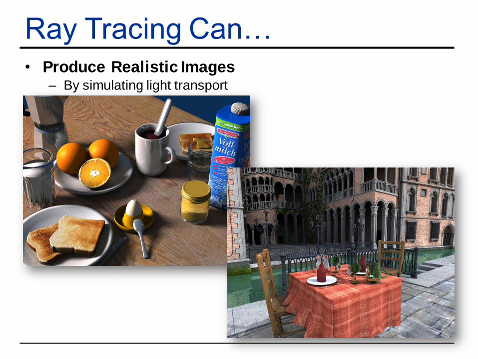
Ray Tracing Can…• Produce Realistic Images
– By simulating light transport
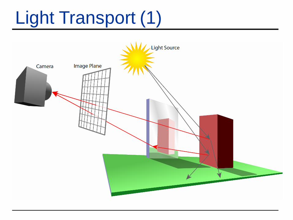
Light Transport (1)
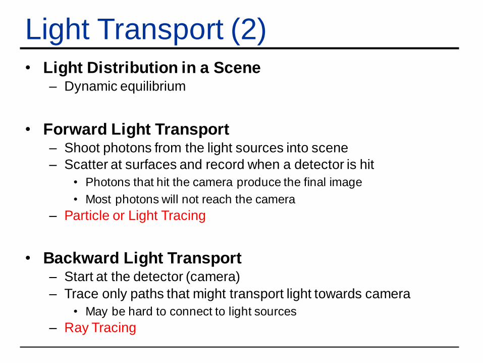
Light Transport (2)• Light Distribution in a Scene
– Dynamic equilibrium
• Forward Light Transport – Shoot photons from the light sources into scene
– Scatter at surfaces and record when a detector is hit
• Photons that hit the camera produce the final image
• Most photons will not reach the camera
– Particle or Light Tracing
• Backward Light Transport– Start at the detector (camera)
– Trace only paths that might transport light towards camera
• May be hard to connect to light sources
– Ray Tracing
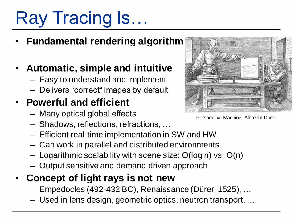
Ray Tracing Is…• Fundamental rendering algorithm
• Automatic, simple and intuitive– Easy to understand and implement
– Delivers “correct“ images by default
• Powerful and efficient– Many optical global effects
– Shadows, reflections, refractions, …
– Efficient real-time implementation in SW and HW
– Can work in parallel and distributed environments
– Logarithmic scalability with scene size: O(log n) vs. O(n)
– Output sensitive and demand driven approach
• Concept of light rays is not new– Empedocles (492-432 BC), Renaissance (Dürer, 1525), …
– Used in lens design, geometric optics, neutron transport, …
Perspective Machine, Albrecht Dürer
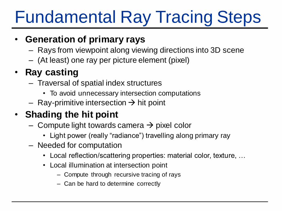
Fundamental Ray Tracing Steps• Generation of primary rays
– Rays from viewpoint along viewing directions into 3D scene
– (At least) one ray per picture element (pixel)
• Ray casting– Traversal of spatial index structures
• To avoid unnecessary intersection computations
– Ray-primitive intersection → hit point
• Shading the hit point– Compute light towards camera → pixel color
• Light power (really “radiance”) travelling along primary ray
– Needed for computation
• Local reflection/scattering properties: material color, texture, …
• Local illumination at intersection point
– Compute through recursive tracing of rays
– Can be hard to determine correctly
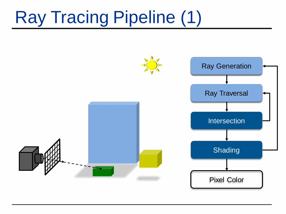
Ray Tracing Pipeline (1)
Ray Generation
Ray Traversal
Intersection
Shading
Pixel Color
Ray Generation
Ray Traversal
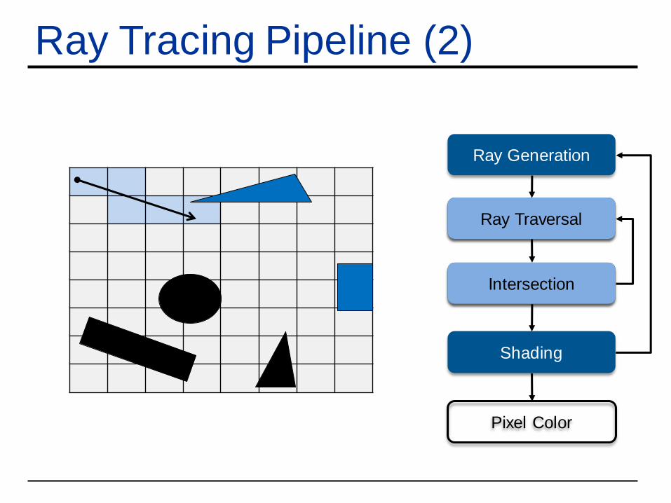
Ray Tracing Pipeline (2)
Ray Generation
Ray Traversal
Intersection
Shading
Pixel Color
Ray Traversal
Intersection
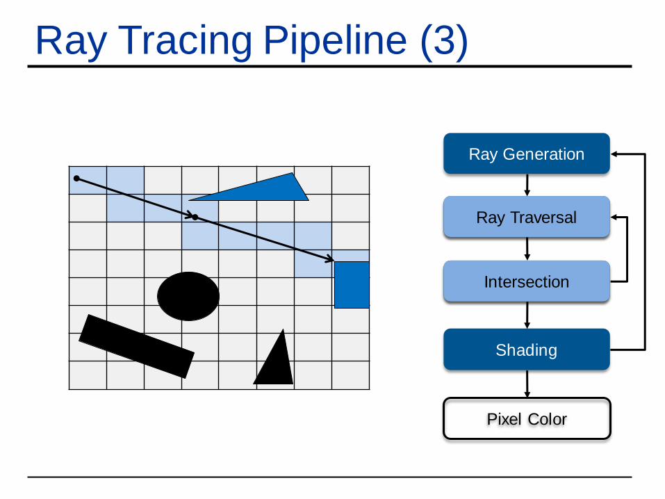
Ray Tracing Pipeline (3)
Ray Generation
Ray Traversal
Intersection
Shading
Pixel Color
Ray Traversal
Intersection
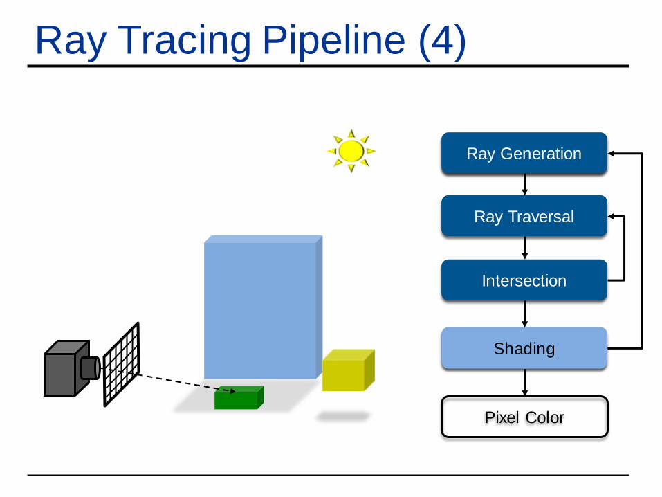
Ray Tracing Pipeline (4)
Ray Generation
Ray Traversal
Intersection
Shading
Pixel Color
Ray Generation
Shading
Ray Traversal
Intersection
Ray Generation
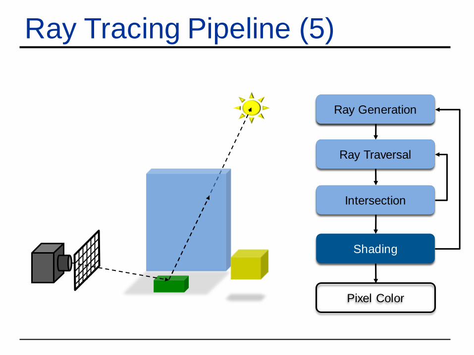
Ray Tracing Pipeline (5)
Ray Generation
Ray Traversal
Intersection
Shading
Pixel Color
Ray Generation
Shading
Ray Traversal
Intersection
Ray Generation

Ray Tracing Pipeline (6)
Ray Generation
Ray Traversal
Intersection
Shading
Pixel Color
Ray Generation
Shading
Ray Traversal
Intersection
Ray Generation
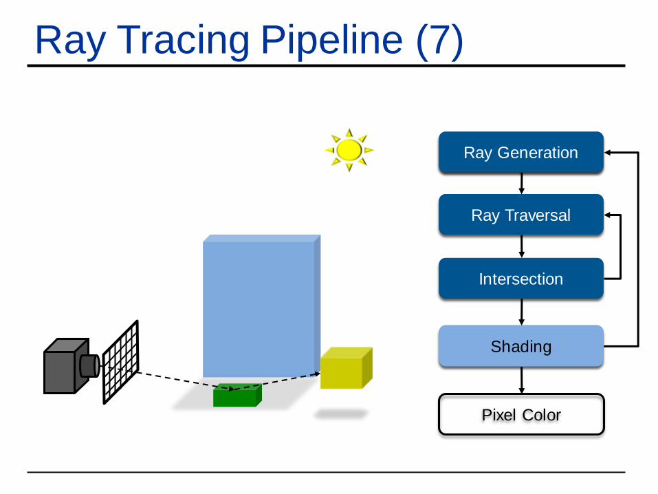
Ray Tracing Pipeline (7)
Ray Generation
Ray Traversal
Intersection
Shading
Pixel Color
Ray Generation
Shading
Ray Traversal
Intersection
Ray Generation

Ray Tracing Pipeline (8)
Ray Generation
Ray Traversal
Intersection
Shading
Pixel Color
Ray Generation
Shading
Ray Traversal
Intersection
Ray Generation
Pixel Color
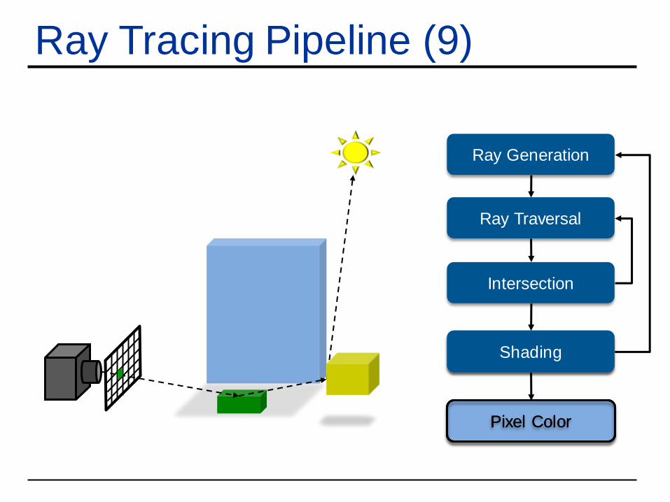
Ray Tracing Pipeline (9)
Ray Generation
Ray Traversal
Intersection
Shading
Pixel Color
Shading
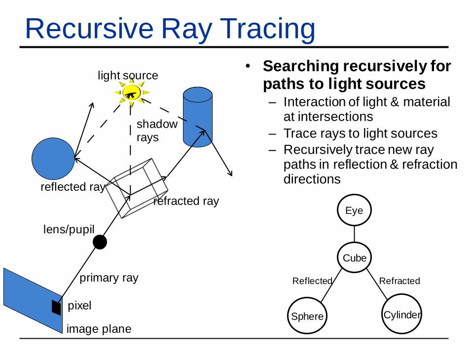
Recursive Ray Tracing• Searching recursively for
paths to light sources– Interaction of light & material
at intersections
– Trace rays to light sources
– Recursively trace new ray paths in reflection & refractiondirections
image plane
pixel
lens/pupil
refracted ray
reflected ray
primary ray
shadowrays
light source
Sphere Cylinder
Cube
Reflected
Eye
Refracted
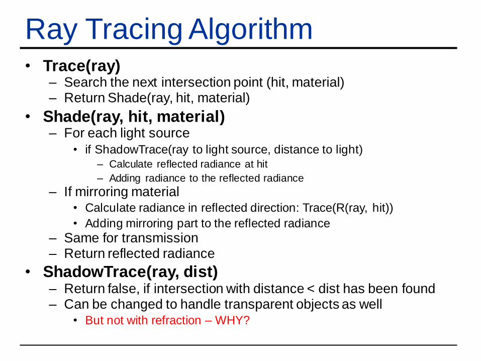
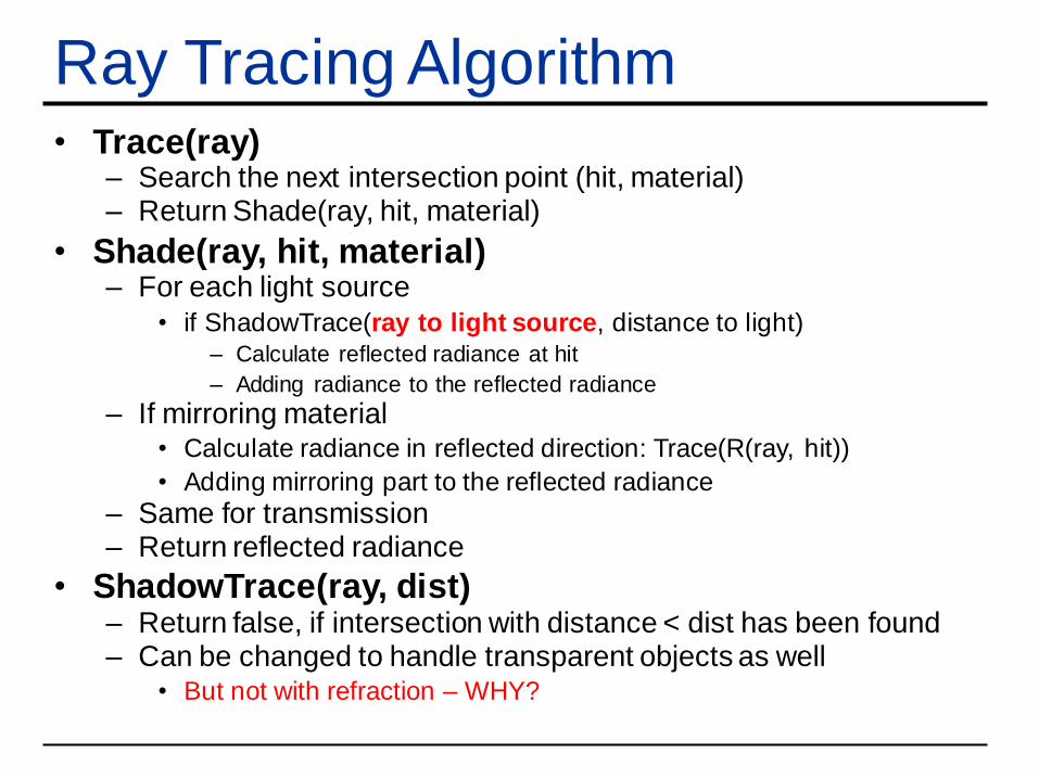
Ray Tracing Algorithm• Trace(ray)
– Search the next intersection point (hit, material)– Return Shade(ray, hit, material)
• Shade(ray, hit, material)– For each light source
• if ShadowTrace(ray to light source, distance to light)– Calculate reflected radiance at hit
– Adding radiance to the reflected radiance
– If mirroring material• Calculate radiance in reflected direction: Trace(R(ray, hit))
• Adding mirroring part to the reflected radiance
– Same for transmission– Return reflected radiance
• ShadowTrace(ray, dist)– Return false, if intersection with distance < dist has been found– Can be changed to handle transparent objects as well
• But not with refraction – WHY?
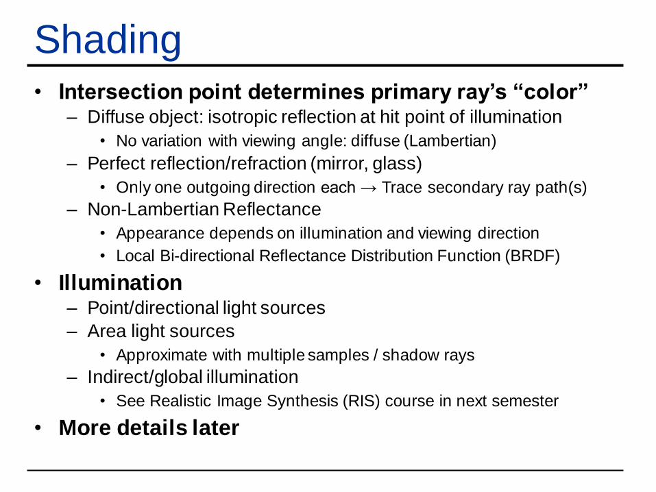
Shading• Intersection point determines primary ray’s “color”
– Diffuse object: isotropic reflection at hit point of illumination
• No variation with viewing angle: diffuse (Lambertian)
– Perfect reflection/refraction (mirror, glass)
• Only one outgoing direction each → Trace secondary ray path(s)
– Non-Lambertian Reflectance
• Appearance depends on illumination and viewing direction
• Local Bi-directional Reflectance Distribution Function (BRDF)
• Illumination– Point/directional light sources
– Area light sources
• Approximate with multiple samples / shadow rays
– Indirect/global illumination
• See Realistic Image Synthesis (RIS) course in next semester
• More details later
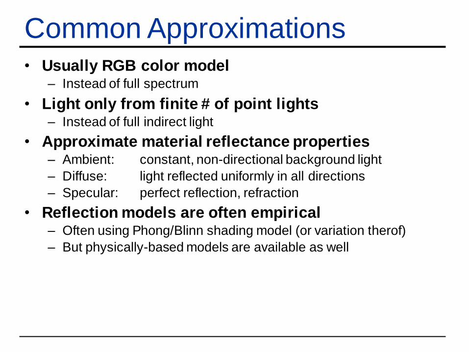
Common Approximations• Usually RGB color model
– Instead of full spectrum
• Light only from finite # of point lights – Instead of full indirect light
• Approximate material reflectance properties– Ambient: constant, non-directional background light
– Diffuse: light reflected uniformly in all directions
– Specular: perfect reflection, refraction
• Reflection models are often empirical– Often using Phong/Blinn shading model (or variation therof)
– But physically-based models are available as well
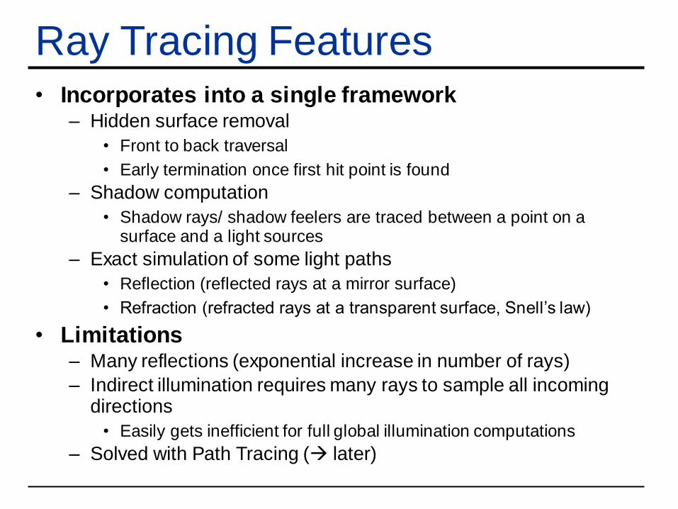
Ray Tracing Features• Incorporates into a single framework
– Hidden surface removal
• Front to back traversal
• Early termination once first hit point is found
– Shadow computation
• Shadow rays/ shadow feelers are traced between a point on a surface and a light sources
– Exact simulation of some light paths
• Reflection (reflected rays at a mirror surface)
• Refraction (refracted rays at a transparent surface, Snell’s law)
• Limitations– Many reflections (exponential increase in number of rays)
– Indirect illumination requires many rays to sample all incoming directions
• Easily gets inefficient for full global illumination computations
– Solved with Path Tracing (→ later)
Ray Tracing Can…• Produce Realistic Images
– By simulating light transport
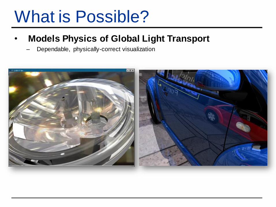
What is Possible?• Models Physics of Global Light Transport
– Dependable, physically-correct visualization
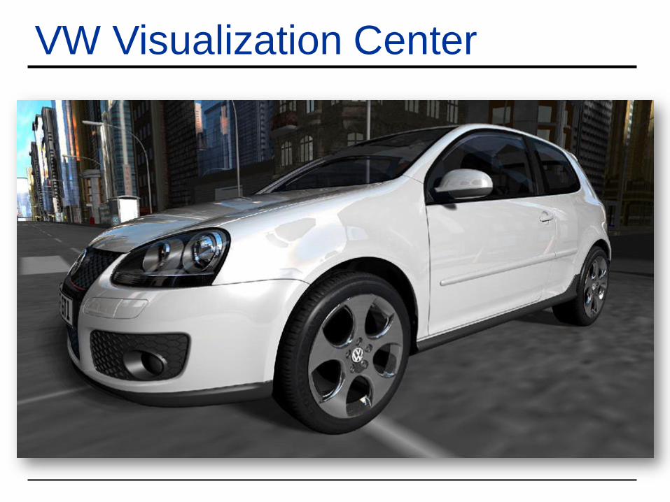
VW Visualization Center
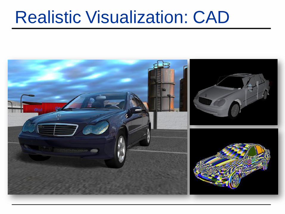
Realistic Visualization: CAD
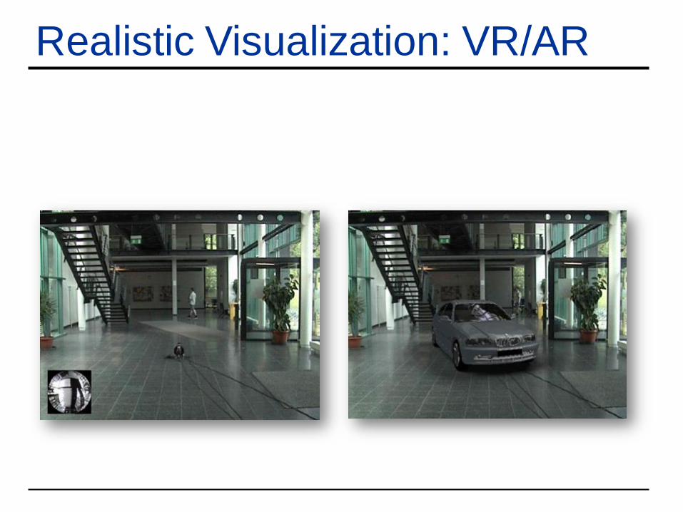
Realistic Visualization: VR/AR
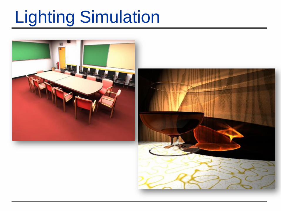
Lighting Simulation
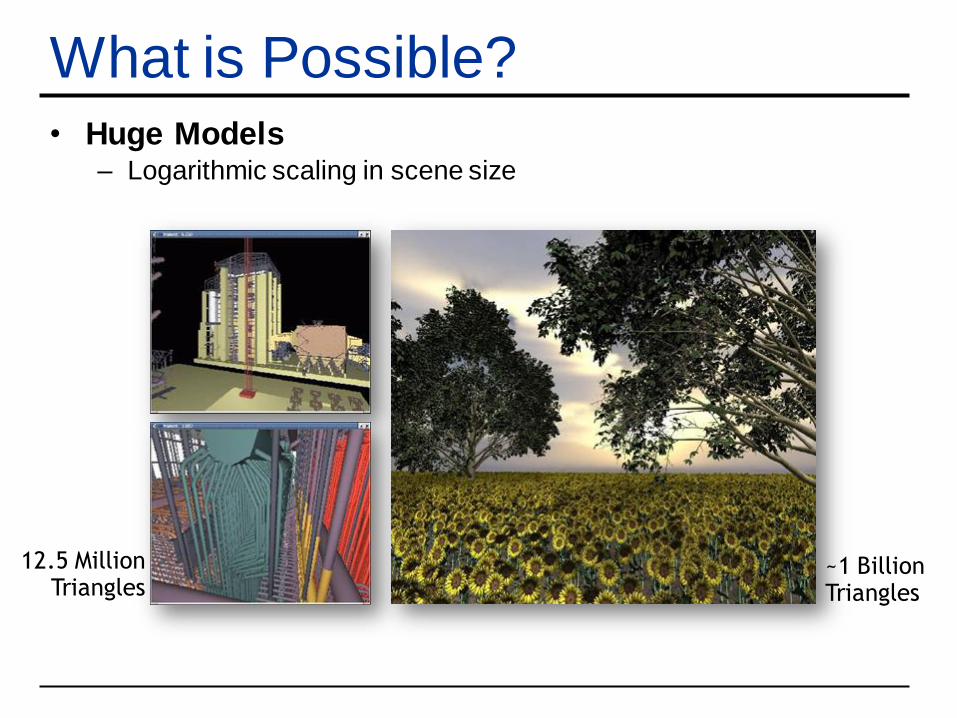
What is Possible?• Huge Models
– Logarithmic scaling in scene size
12.5 MillionTriangles
~1 BillionTriangles
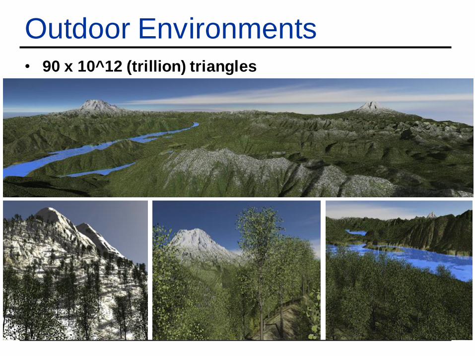
Outdoor Environments• 90 x 10^12 (trillion) triangles
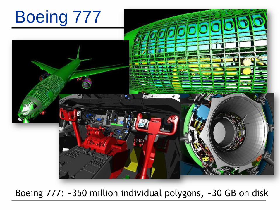
Boeing 777
Boeing 777: ~350 million individual polygons, ~30 GB on disk
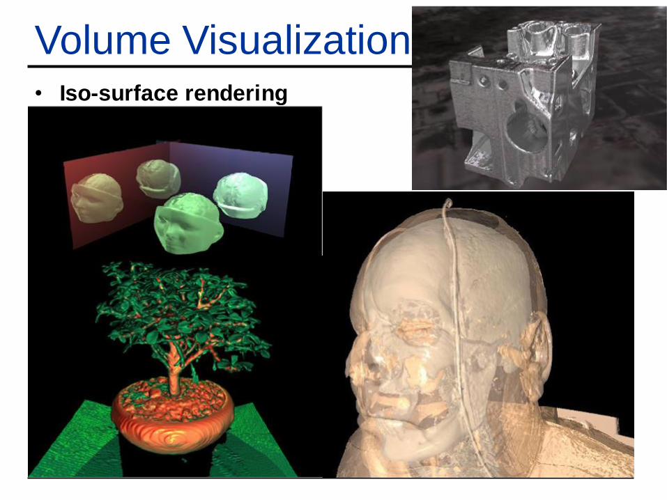
Volume Visualization• Iso-surface rendering
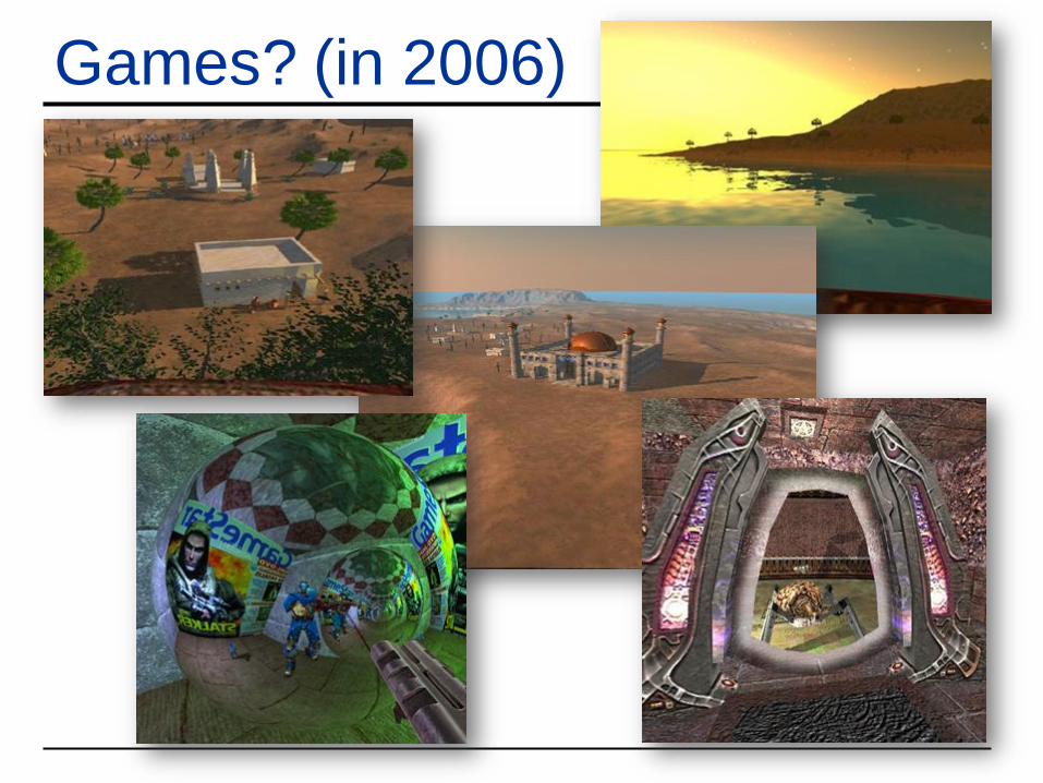
Games? (in 2006)
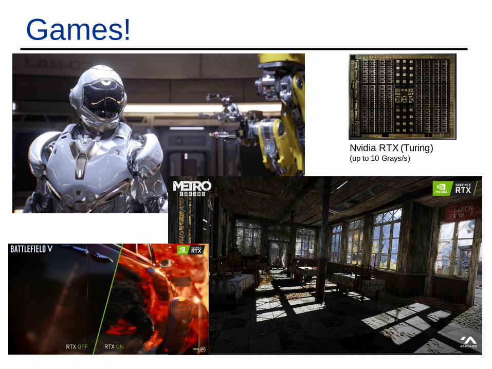
Games!
Nvidia RTX (Turing)(up to 10 Grays/s)
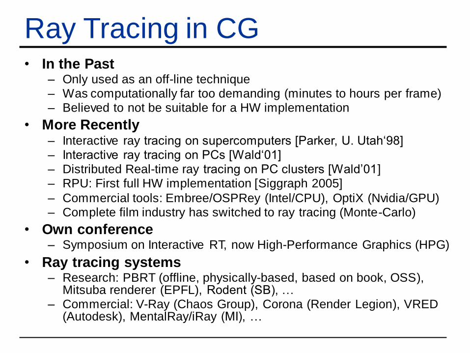
Ray Tracing in CG• In the Past
– Only used as an off-line technique– Was computationally far too demanding (minutes to hours per frame)– Believed to not be suitable for a HW implementation
• More Recently– Interactive ray tracing on supercomputers [Parker, U. Utah‘98]– Interactive ray tracing on PCs [Wald‘01]– Distributed Real-time ray tracing on PC clusters [Wald’01]– RPU: First full HW implementation [Siggraph 2005]
– Commercial tools: Embree/OSPRey (Intel/CPU), OptiX (Nvidia/GPU)– Complete film industry has switched to ray tracing (Monte-Carlo)
• Own conference– Symposium on Interactive RT, now High-Performance Graphics (HPG)
• Ray tracing systems– Research: PBRT (offline, physically-based, based on book, OSS),
Mitsuba renderer (EPFL), Rodent (SB), …– Commercial: V-Ray (Chaos Group), Corona (Render Legion), VRED
(Autodesk), MentalRay/iRay (MI), …
Ray Casting Outside CG• Tracing/Casting a ray
– Special type of query
• “Is there a primitive along a ray”
• “How far is the closest primitive”
• Other uses than rendering– Volume computation
– Sound waves tracing
– Collision detection
– …
RAY-PRIMITIVE
INTERSECTIONS
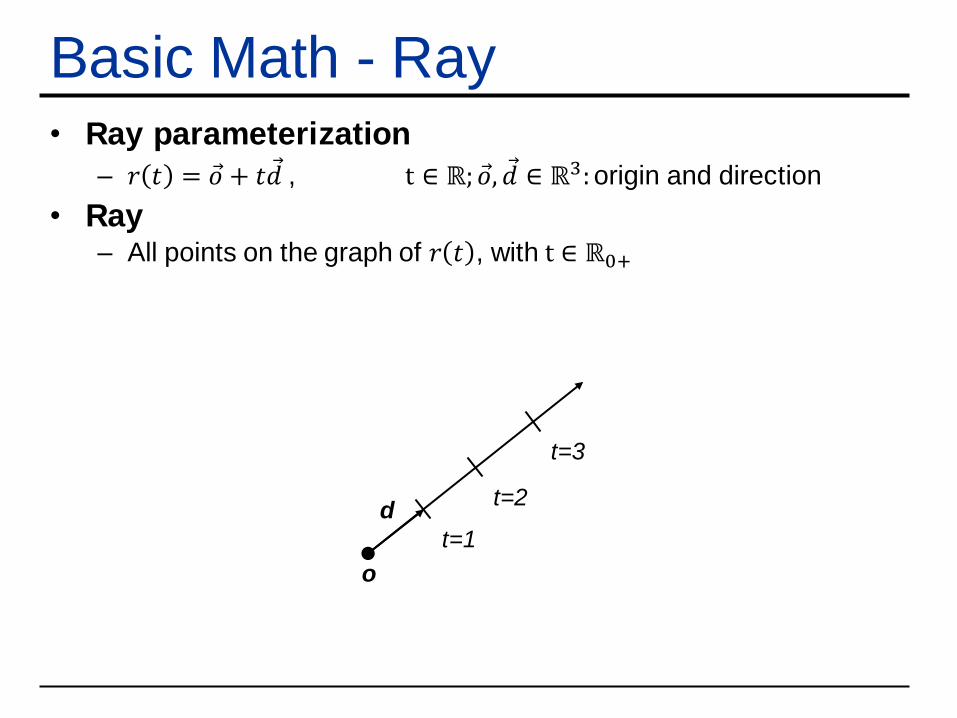
Basic Math - Ray• Ray parameterization
– 𝑟 𝑡 = Ԧ𝑜 + 𝑡 Ԧ𝑑 , t ∈ ℝ; Ԧ𝑜, Ԧ𝑑 ∈ ℝ3:origin and direction
• Ray– All points on the graph of 𝑟 𝑡 , with t ∈ ℝ0+
o
d
t=1
t=3
t=2
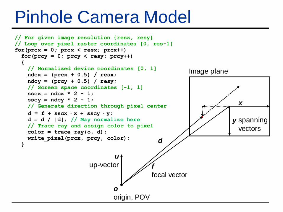
Pinhole Camera Model// For given image resolution {resx, resy}
// Loop over pixel raster coordinates [0, res-1]
for(prcx = 0; prcx < resx; prcx++)
for(prcy = 0; prcy < resy; prcy++)
{
// Normalized device coordinates [0, 1]
ndcx = (prcx + 0.5) / resx;
ndcy = (prcy + 0.5) / resy;
// Screen space coordinates [-1, 1]
sscx = ndcx * 2 - 1;
sscy = ndcy * 2 - 1;
// Generate direction through pixel center
d = f + sscx x + sscy y;d = d / |d|; // May normalize here
// Trace ray and assign color to pixel
color = trace_ray(o, d);
write_pixel(prcx, prcy, color);
}
x
spanning
vectorsy
o
origin, POV
u
up-vector f
focal vector
d
Image plane
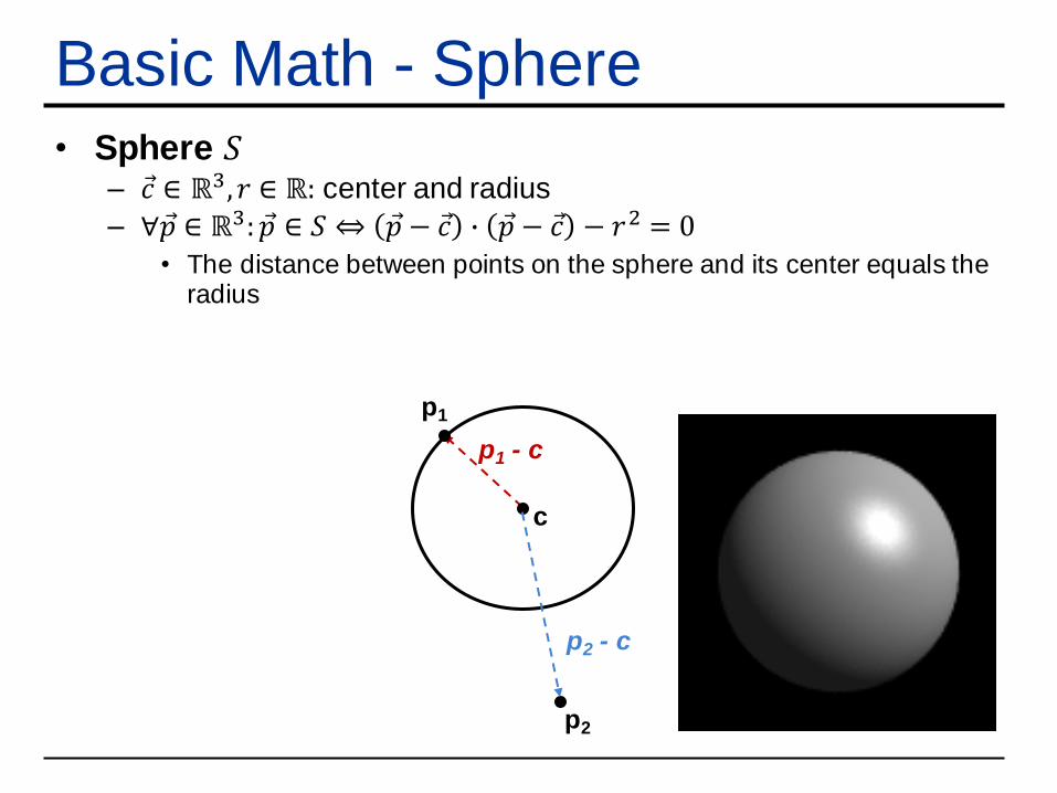
Basic Math - Sphere• Sphere 𝑆
– Ԧ𝑐 ∈ ℝ3, 𝑟 ∈ ℝ: center and radius
– ∀ Ԧ𝑝 ∈ ℝ3: Ԧ𝑝 ∈ 𝑆 ⇔ Ԧ𝑝 − Ԧ𝑐 ∙ Ԧ𝑝 − Ԧ𝑐 − 𝑟2 = 0
• The distance between points on the sphere and its center equals the radius
c
p1
p1 - c
p2 - c
p2
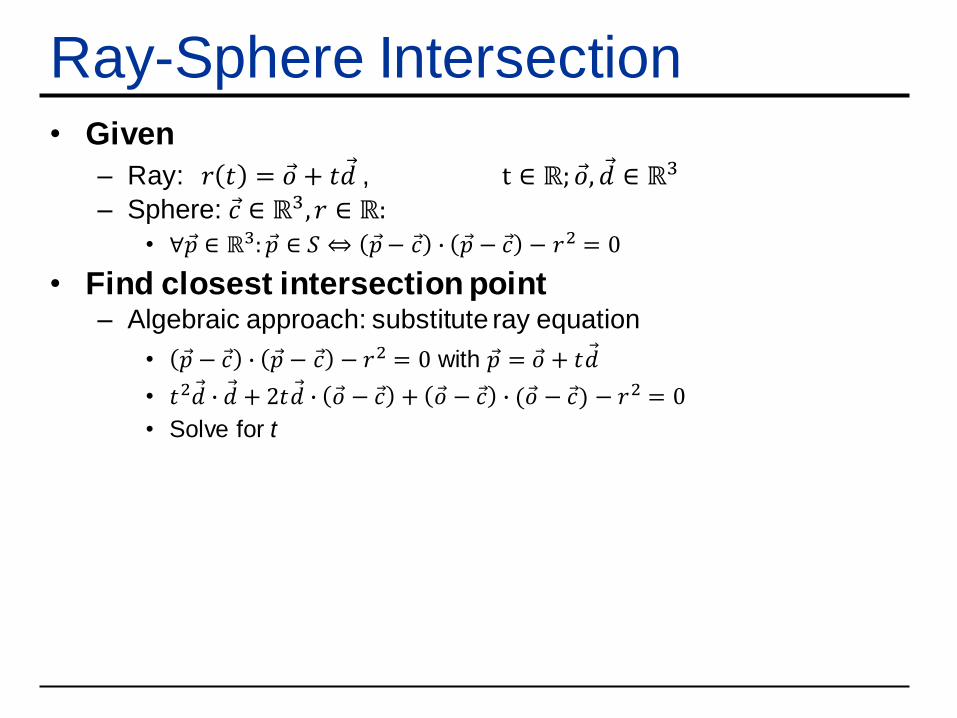
Ray-Sphere Intersection• Given
– Ray: 𝑟 𝑡 = Ԧ𝑜 + 𝑡 Ԧ𝑑 , t ∈ ℝ; Ԧ𝑜, Ԧ𝑑 ∈ ℝ3
– Sphere: Ԧ𝑐 ∈ ℝ3, 𝑟 ∈ ℝ:
• ∀ Ԧ𝑝 ∈ ℝ3: Ԧ𝑝 ∈ 𝑆 ⇔ Ԧ𝑝− Ԧ𝑐 ∙ Ԧ𝑝 − Ԧ𝑐 − 𝑟2 = 0
• Find closest intersection point– Algebraic approach: substitute ray equation
• Ԧ𝑝 − Ԧ𝑐 ∙ Ԧ𝑝 − Ԧ𝑐 − 𝑟2 = 0 with Ԧ𝑝 = Ԧ𝑜 + 𝑡 Ԧ𝑑
• 𝑡2 Ԧ𝑑 ∙ Ԧ𝑑 + 2𝑡 Ԧ𝑑 ∙ Ԧ𝑜 − Ԧ𝑐 + Ԧ𝑜 − Ԧ𝑐 ∙ ( Ԧ𝑜 − Ԧ𝑐) − 𝑟2 = 0
• Solve for t
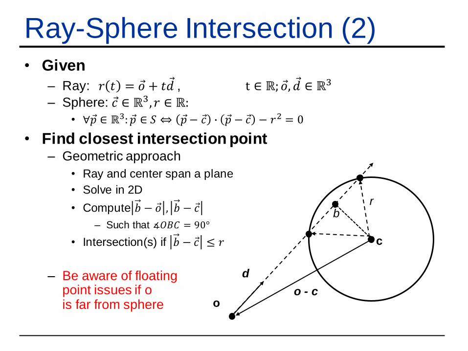
Ray-Sphere Intersection (2)• Given
– Ray: 𝑟 𝑡 = Ԧ𝑜 + 𝑡 Ԧ𝑑 , t ∈ ℝ; Ԧ𝑜, Ԧ𝑑 ∈ ℝ3
– Sphere: Ԧ𝑐 ∈ ℝ3, 𝑟 ∈ ℝ:
• ∀ Ԧ𝑝 ∈ ℝ3: Ԧ𝑝 ∈ 𝑆 ⇔ Ԧ𝑝− Ԧ𝑐 ∙ Ԧ𝑝 − Ԧ𝑐 − 𝑟2 = 0
• Find closest intersection point– Geometric approach
• Ray and center span a plane
• Solve in 2D
• Compute 𝑏 − Ԧ𝑜 , 𝑏 − Ԧ𝑐
– Such that ∡𝑂𝐵𝐶 = 90°
• Intersection(s) if 𝑏 − Ԧ𝑐 ≤ 𝑟
– Be aware of floatingpoint issues if ois far from sphere
c
r
d
oo - c
b
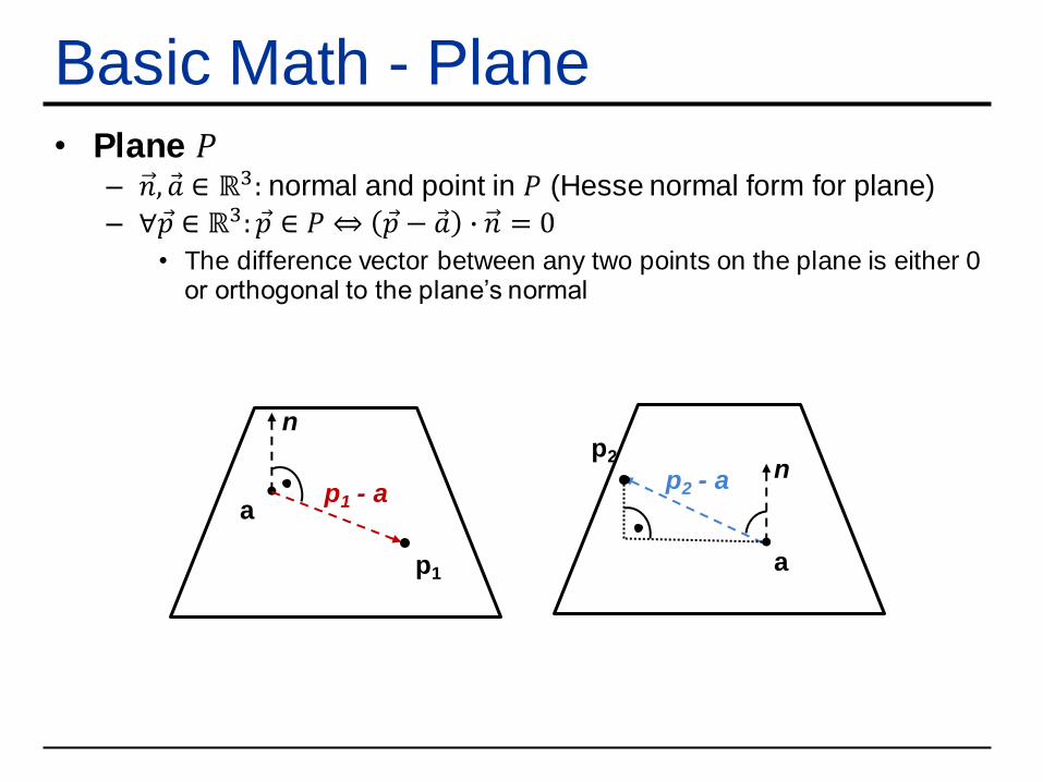
Basic Math - Plane• Plane 𝑃
– 𝑛, Ԧ𝑎 ∈ ℝ3: normal and point in 𝑃 (Hesse normal form for plane)
– ∀ Ԧ𝑝 ∈ ℝ3: Ԧ𝑝 ∈ 𝑃 ⇔ Ԧ𝑝 − Ԧ𝑎 ∙ 𝑛 = 0
• The difference vector between any two points on the plane is either 0 or orthogonal to the plane’s normal
n
a
p1
p1 - an
a
p2
p2 - a
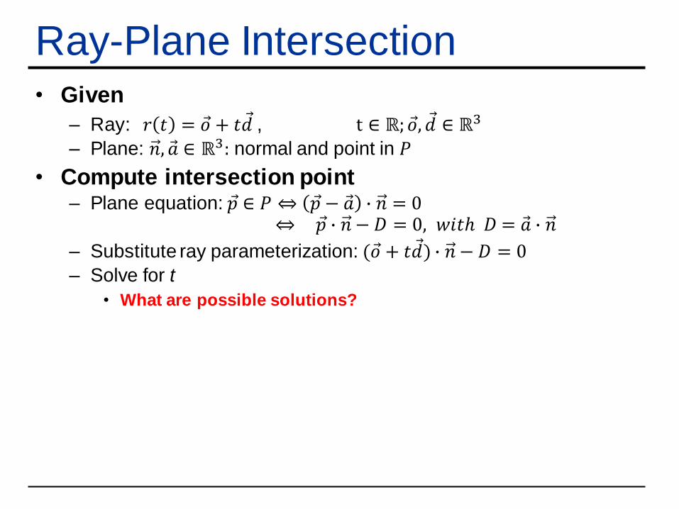
Ray-Plane Intersection• Given
– Ray: 𝑟 𝑡 = Ԧ𝑜 + 𝑡 Ԧ𝑑 , t ∈ ℝ; Ԧ𝑜, Ԧ𝑑 ∈ ℝ3
– Plane: 𝑛, Ԧ𝑎 ∈ ℝ3: normal and point in 𝑃
• Compute intersection point– Plane equation: Ԧ𝑝 ∈ 𝑃 ⇔ Ԧ𝑝 − Ԧ𝑎 ∙ 𝑛 = 0
⇔ Ԧ𝑝 ∙ 𝑛 − 𝐷 = 0, 𝑤𝑖𝑡ℎ 𝐷 = Ԧ𝑎 ∙ 𝑛
– Substitute ray parameterization: ( Ԧ𝑜 + 𝑡 Ԧ𝑑) ∙ 𝑛 − 𝐷 = 0
– Solve for t
• What are possible solutions?
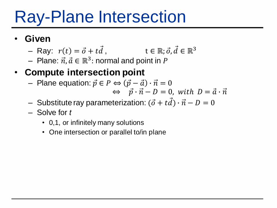
Ray-Plane Intersection• Given
– Ray: 𝑟 𝑡 = Ԧ𝑜 + 𝑡 Ԧ𝑑 , t ∈ ℝ; Ԧ𝑜, Ԧ𝑑 ∈ ℝ3
– Plane: 𝑛, Ԧ𝑎 ∈ ℝ3: normal and point in 𝑃
• Compute intersection point– Plane equation: Ԧ𝑝 ∈ 𝑃 ⇔ Ԧ𝑝 − Ԧ𝑎 ∙ 𝑛 = 0
⇔ Ԧ𝑝 ∙ 𝑛 − 𝐷 = 0, 𝑤𝑖𝑡ℎ 𝐷 = Ԧ𝑎 ∙ 𝑛
– Substitute ray parameterization: ( Ԧ𝑜 + 𝑡 Ԧ𝑑) ∙ 𝑛 − 𝐷 = 0
– Solve for t
• 0,1, or infinitely many solutions
• One intersection or parallel to/in plane
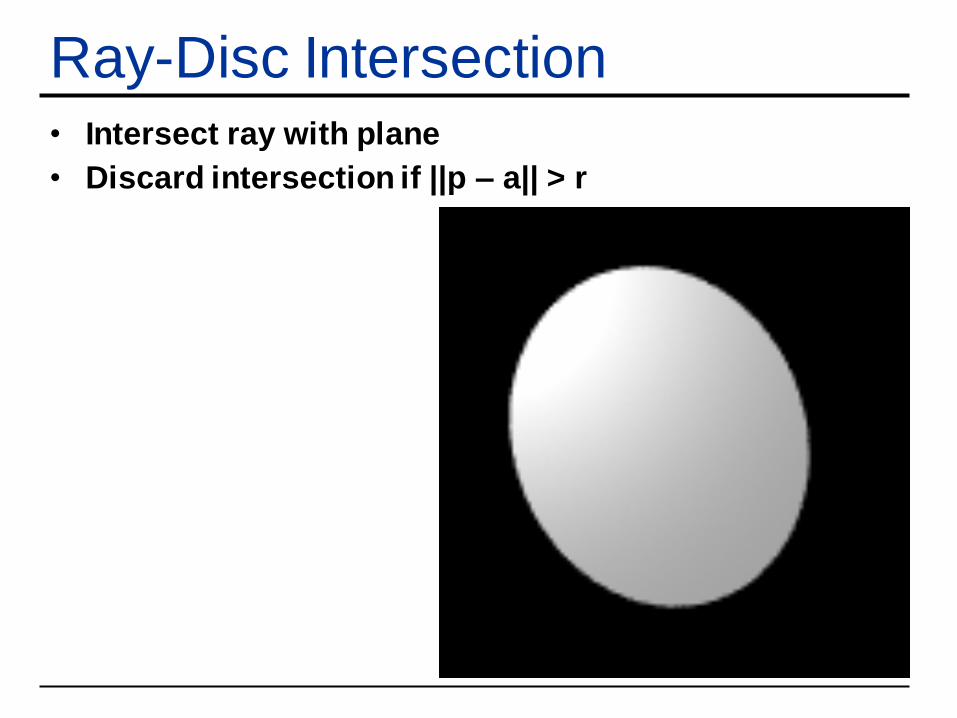
Ray-Disc Intersection• Intersect ray with plane
• Discard intersection if ||p – a|| > r
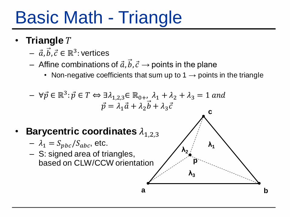
Basic Math - Triangle• Triangle 𝑇
– Ԧ𝑎,𝑏, Ԧ𝑐 ∈ ℝ3: vertices
– Affine combinations of Ԧ𝑎,𝑏, Ԧ𝑐 → points in the plane
• Non-negative coefficients that sum up to 1 → points in the triangle
– ∀ Ԧ𝑝 ∈ ℝ3: Ԧ𝑝 ∈ 𝑇 ⇔ ∃𝜆1,2,3∈ ℝ0+, 𝜆1 +𝜆2 + 𝜆3 = 1 𝑎𝑛𝑑
Ԧ𝑝 = 𝜆1 Ԧ𝑎 + 𝜆2𝑏 + 𝜆3 Ԧ𝑐
• Barycentric coordinates 𝜆1,2,3– 𝜆1 = 𝑆𝑝𝑏𝑐/𝑆𝑎𝑏𝑐, etc.
– S: signed area of triangles,based on CLW/CCW orientation
c
a b
p
λ1
λ3
λ2
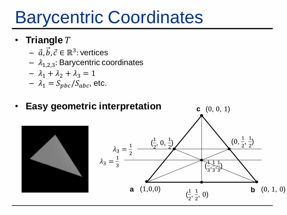
Barycentric Coordinates• Triangle 𝑇
– Ԧ𝑎,𝑏, Ԧ𝑐 ∈ ℝ3: vertices
– 𝜆1,2,3: Barycentric coordinates
– 𝜆1 + 𝜆2 + 𝜆3 = 1– 𝜆1 = 𝑆𝑝𝑏𝑐/𝑆𝑎𝑏𝑐, etc.
• Easy geometric interpretation
(1,0,0) (0, 1, 0)
(0, 0, 1)
𝜆3 =1
2
(0, 1
2, 1
2)
(1
2, 1
2, 0)
(1
2, 0,
1
2)
(1
3,1
3,1
3)
𝜆3 =1
3
c
a b
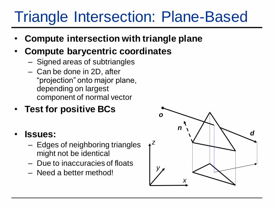
Triangle Intersection: Plane-Based
• Compute intersection with triangle plane
• Compute barycentric coordinates– Signed areas of subtriangles
– Can be done in 2D, after “projection” onto major plane,depending on largestcomponent of normal vector
• Test for positive BCs
• Issues:– Edges of neighboring triangles
might not be identical
– Due to inaccuracies of floats
– Need a better method!
n
o
d
x
y
z
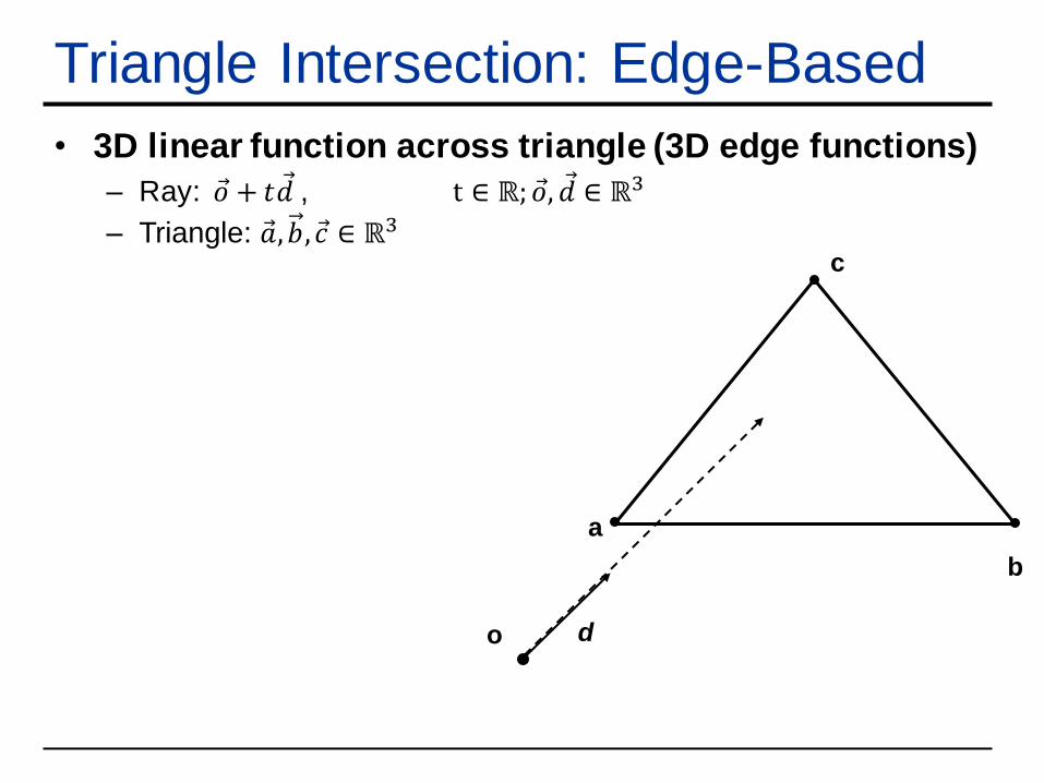
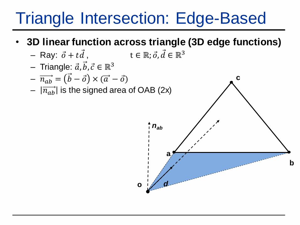
Triangle Intersection: Edge-Based
• 3D linear function across triangle (3D edge functions)
– Ray: Ԧ𝑜 + 𝑡 Ԧ𝑑 , t ∈ ℝ; Ԧ𝑜, Ԧ𝑑 ∈ ℝ3
– Triangle: Ԧ𝑎,𝑏, Ԧ𝑐 ∈ ℝ3
b
do
c
a
• 3D linear function across triangle (3D edge functions)
– Ray: Ԧ𝑜 + 𝑡 Ԧ𝑑 , t ∈ ℝ; Ԧ𝑜, Ԧ𝑑 ∈ ℝ3
– Triangle: Ԧ𝑎,𝑏, Ԧ𝑐 ∈ ℝ3
– 𝑛𝑎𝑏 = 𝑏 − Ԧ𝑜 × (𝑎 − Ԧ𝑜)
– 𝑛𝑎𝑏 is the signed area of OAB (2x)
b
do
c
a
nab
Triangle Intersection: Edge-Based
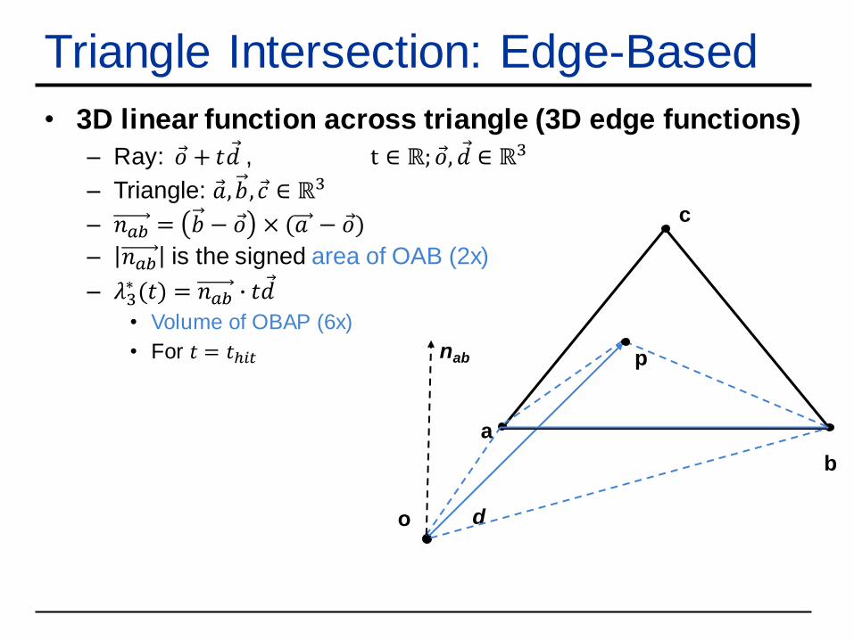
Triangle Intersection: Edge-Based
• 3D linear function across triangle (3D edge functions)
– Ray: Ԧ𝑜 + 𝑡 Ԧ𝑑 , t ∈ ℝ; Ԧ𝑜, Ԧ𝑑 ∈ ℝ3
– Triangle: Ԧ𝑎,𝑏, Ԧ𝑐 ∈ ℝ3
– 𝑛𝑎𝑏 = 𝑏 − Ԧ𝑜 × (𝑎 − Ԧ𝑜)
– 𝑛𝑎𝑏 is the signed area of OAB (2x)
– 𝜆3∗ (𝑡) = 𝑛𝑎𝑏 ∙ 𝑡 Ԧ𝑑
• Volume of OBAP (6x)
• For 𝑡 = 𝑡ℎ𝑖𝑡
b
do
c
a
nab p
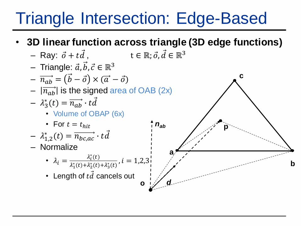
Triangle Intersection: Edge-Based
• 3D linear function across triangle (3D edge functions)
– Ray: Ԧ𝑜 + 𝑡 Ԧ𝑑 , t ∈ ℝ; Ԧ𝑜, Ԧ𝑑 ∈ ℝ3
– Triangle: Ԧ𝑎,𝑏, Ԧ𝑐 ∈ ℝ3
– 𝑛𝑎𝑏 = 𝑏 − Ԧ𝑜 × (𝑎 − Ԧ𝑜)
– 𝑛𝑎𝑏 is the signed area of OAB (2x)
– 𝜆3∗ (𝑡) = 𝑛𝑎𝑏 ∙ 𝑡 Ԧ𝑑
• Volume of OBAP (6x)
• For 𝑡 = 𝑡ℎ𝑖𝑡
– 𝜆1,2∗ (𝑡) = 𝑛𝑏𝑐,𝑎𝑐 ∙ 𝑡 Ԧ𝑑
– Normalize
• 𝜆𝑖 =𝜆𝑖∗(𝑡)
𝜆1∗(𝑡)+𝜆2
∗(𝑡)+𝜆3∗(𝑡)
, 𝑖 = 1,2,3
• Length of 𝑡 Ԧ𝑑 cancels out
b
do
c
a
nab p
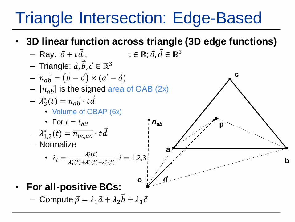
Triangle Intersection: Edge-Based
• 3D linear function across triangle (3D edge functions)
– Ray: Ԧ𝑜 + 𝑡 Ԧ𝑑 , t ∈ ℝ; Ԧ𝑜, Ԧ𝑑 ∈ ℝ3
– Triangle: Ԧ𝑎,𝑏, Ԧ𝑐 ∈ ℝ3
– 𝑛𝑎𝑏 = 𝑏 − Ԧ𝑜 × (𝑎 − Ԧ𝑜)
– 𝑛𝑎𝑏 is the signed area of OAB (2x)
– 𝜆3∗ (𝑡) = 𝑛𝑎𝑏 ∙ 𝑡 Ԧ𝑑
• Volume of OBAP (6x)
• For 𝑡 = 𝑡ℎ𝑖𝑡
– 𝜆1,2∗ (𝑡) = 𝑛𝑏𝑐,𝑎𝑐 ∙ 𝑡 Ԧ𝑑
– Normalize
• 𝜆𝑖 =𝜆𝑖∗(𝑡)
𝜆1∗(𝑡)+𝜆2
∗(𝑡)+𝜆3∗(𝑡)
, 𝑖 = 1,2,3
• For all-positive BCs:
– Compute Ԧ𝑝 = 𝜆1 Ԧ𝑎 + 𝜆2𝑏 + 𝜆3 Ԧ𝑐
b
do
c
a
pnab
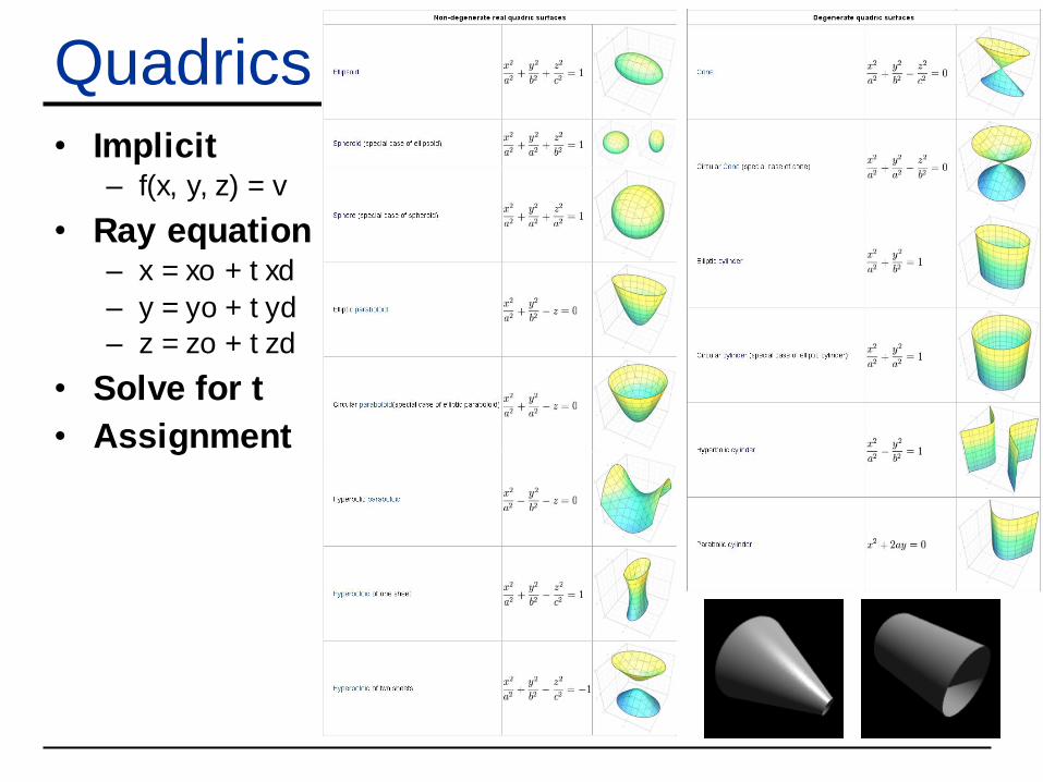
Quadrics• Implicit
– f(x, y, z) = v
• Ray equation– x = xo + t xd
– y = yo + t yd
– z = zo + t zd
• Solve for t
• Assignment
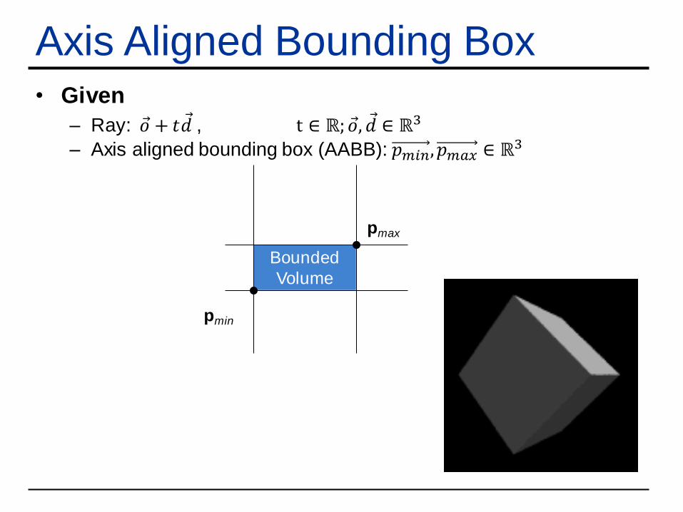
Axis Aligned Bounding Box• Given
– Ray: Ԧ𝑜 + 𝑡 Ԧ𝑑 , t ∈ ℝ; Ԧ𝑜, Ԧ𝑑 ∈ ℝ3
– Axis aligned bounding box (AABB): 𝑝𝑚𝑖𝑛, 𝑝𝑚𝑎𝑥 ∈ ℝ3
Bounded
Volume
pmin
pmax
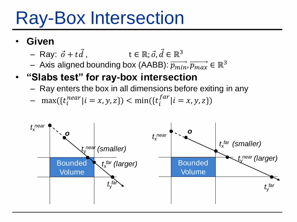
Ray-Box Intersection• Given
– Ray: Ԧ𝑜 + 𝑡 Ԧ𝑑 , t ∈ ℝ; Ԧ𝑜, Ԧ𝑑 ∈ ℝ3
– Axis aligned bounding box (AABB): 𝑝𝑚𝑖𝑛, 𝑝𝑚𝑎𝑥 ∈ ℝ3
• “Slabs test” for ray-box intersection– Ray enters the box in all dimensions before exiting in any
– max({𝑡𝑖𝑛𝑒𝑎𝑟|𝑖 = 𝑥, 𝑦, 𝑧}) < min({𝑡𝑖
𝑓𝑎𝑟|𝑖 = 𝑥, 𝑦, 𝑧})
Bounded
Volume
txnear
tynear (smaller)
tyfar
o
txfar (larger) Bounded
Volume
txnear
txfar (smaller)
tyfar
o
tynear (larger)
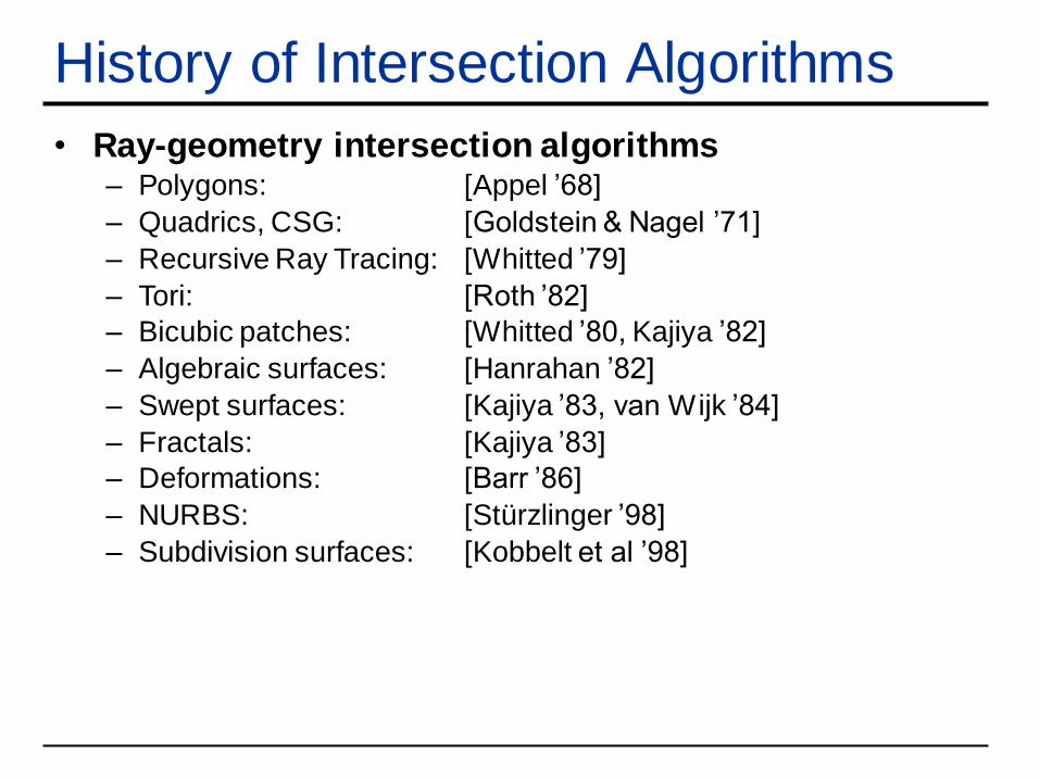
History of Intersection Algorithms
• Ray-geometry intersection algorithms– Polygons: [Appel ’68]
– Quadrics, CSG: [Goldstein & Nagel ’71]
– Recursive Ray Tracing: [Whitted ’79]
– Tori: [Roth ’82]
– Bicubic patches: [Whitted ’80, Kajiya ’82]
– Algebraic surfaces: [Hanrahan ’82]
– Swept surfaces: [Kajiya ’83, van Wijk ’84]
– Fractals: [Kajiya ’83]
– Deformations: [Barr ’86]
– NURBS: [Stürzlinger ’98]
– Subdivision surfaces: [Kobbelt et al ’98]
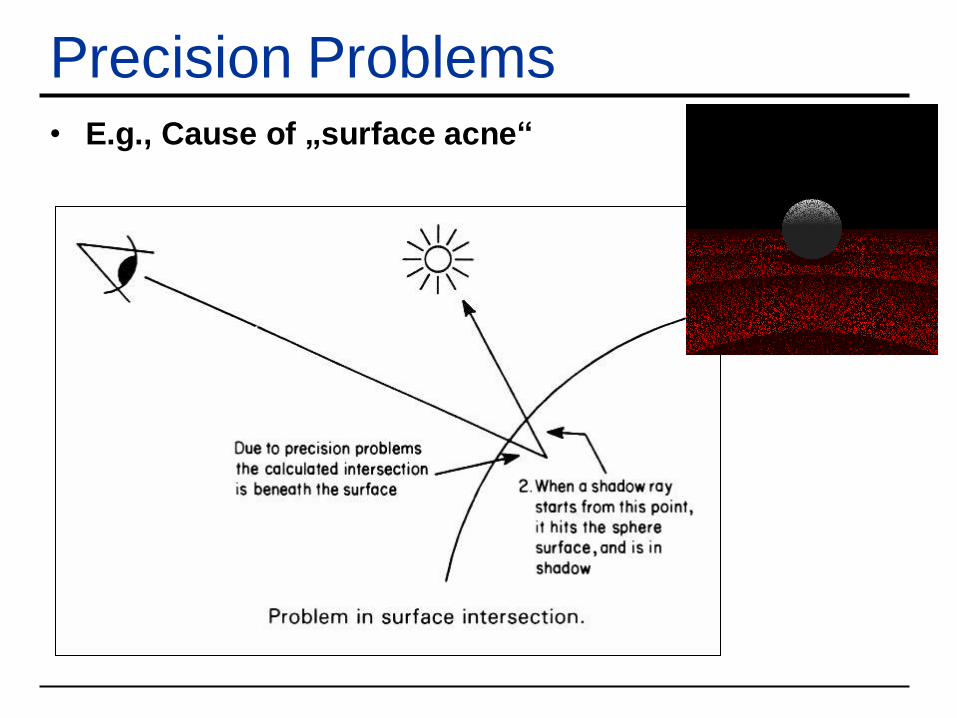
Precision Problems• E.g., Cause of „surface acne“