Computer Algebra and Algebraic. Geometry--Achievements … · 254 G.-M. Greuel a standard part of...

doi:10.1006/jsco.2000.0362Available online at http://www.idealibrary.com on

J. Symbolic Computation (2000) 30, 253–289

Computer Algebra and Algebraic.Geometry—Achievements and Perspectives†

GERT-MARTIN GREUEL‡

Fachbereich Mathematik, Universitat Kaiserslautern, Erwin-Schrodinger-Straße,D – 67663 Kaiserslautern

De computer is niet de steenmaar de slijpsteen der wijzen.(The computer is not the philosopher’s stonebut the philosopher’s whetstone.)Hugo Battus, Rekenen op taal (1989)

1. Preface

In this survey I should like to introduce some concepts of algebraic geometry and try todemonstrate the fruitful interaction between algebraic geometry and computer algebraand, more generally, between mathematics and computer science. One of the aims ofthis paper is to show, by means of examples, the usefulness of computer algebra tomathematical research.

Computer algebra itself is a highly diversified discipline with applications to variousareas of mathematics; many of these may be found in numerous research papers, proceed-ings or textbooks (cf. Buchberger and Winkler, 1998; Cohen et al., 1999; Matzat et al.,1998; ISSAC, 1988–1998). Here, I concentrate mainly on Grobner bases and leave asidemany other topics of computer algebra (cf. Davenport et al., 1988; Von zur Gathen andGerhard, 1999; Grabmeier et al., 2000). In particular, I do not mention (multivariate)polynomial factorization, another major and important tool in computational algebraicgeometry. Grobner bases were introduced originally by Buchberger as a computationaltool for testing solvability of a system of polynomial equations, to count the number ofsolutions (with multiplicities) if this number is finite and, more algebraically, to com-pute in the quotient ring modulo the given polynomials. Since then, Grobner bases havebecome the major computational tool, not only in algebraic geometry.

The importance of Grobner bases for mathematical research in algebraic geometryis obvious and nowadays their use needs hardly any justification. Indeed, chapters onGrobner bases and Buchberger’s algorithm (Buchberger, 1965) have been incorporatedin many new textbooks on algebraic geometry such as the books of Cox et al. (1992, 1998)or the recent books of Eisenbud (1995) and Vasconcelos (1998), not to mention textbookswhich are devoted exclusively to Grobner bases, such as Adams and Loustaunou (1994),Becker and Weispfennig (1993) and Froberg (1997).

Computational methods become increasingly important in pure mathematics and theabove-mentioned books have the effect that Grobner bases and their applications become

†This paper is an extended version of an invited talk, delivered at the ISSAC’98 conference at Rostock,13–15 August, 1998.

‡E-mail: [email protected]

0747–7171/00/030253 + 37 $35.00/0 c© 2000 Academic Press

254 G.-M. Greuel

a standard part of university courses on algebraic geometry and commutative algebra.One of the reasons is that these methods, together with very efficient computers, allowthe treatment of non-trivial examples and, moreover, are applicable to non-mathematical,industrial, technical or economical problems. Another reason is that there is a belief thatalgorithms can contribute to a deeper understanding of a problem. The human ideaof “understanding” is clearly part of the historical, cultural and technical status of thesociety and nowadays understanding in mathematics requires more and more algorithmictreatment and computational mastering.

On the other hand, it is also obvious that many of the recent deepest achievements inalgebraic and arithmetic geometry, such as string theory and mirror symmetry (comingfrom physics) or Wiles’ proof of Fermat’s last theorem, just to mention a few, were neitherinspired by nor used computer algebra at all. I just mention this in order to stress that nocomputer algebra system can ever replace, in any significant way, mathematical thinking.

Generally speaking, algorithmic treatment and computational mastering marks not thebeginning but the end of a development and already requires an advanced theoreticalunderstanding. In many cases an algorithm is, however, much more than just a carefulanalysis of known results, it is really a new level of understanding, and an efficientimplementation is, in addition, usually a highly non-trivial task. Furthermore, having acomputer algebra system which has such algorithms implemented and which is easy touse, then becomes a powerful tool for the working mathematician, like a calculator forthe engineer.

In this connection I should like to stress that having Buchberger’s algorithm for com-puting Grobner bases of an ideal is, although indispensable, not much more than having+, −, *, / on a calculator. Nowadays, there exist efficient implementations of very in-volved and sophisticated algorithms (most of them use Grobner bases in an essentialway) allowing the computation of such things as:

• Hilbert polynomials of graded ideals and modules,• free resolutions of finitely generated modules,• Ext, Tor and cohomology groups,• infinitesimal deformations and obstructions of varieties and singularities,• versal deformations of varieties and singularities,• primary decomposition of ideals,• normalization of affine rings,• invariant rings of finite and reductive groups,• Puiseux expansion of plane curve singularities,

not to mention the standard operations like ideal and radical membership, ideal inter-section, ideal quotient and elimination of variables. All the above-mentioned algorithmsare implemented in SINGULAR (Greuel et al., 1990–1998), some of them also in CoCoA(Capani et al., 1995) and Macaulay, resp. Macaulay2 (Bayer and Stillman, 1982–1990resp. Grayson and Stillmann, 1996), to mention computer algebra systems which aredesigned for use in algebraic geometry and commutative algebra. Even general purposeand commercial systems such as Mathematica, Maple, MuPad etc. offer Grobner basesand, based on this, libraries treating special problems in algebra and geometry.

It is well-acknowledged that Grobner bases and Buchberger’s algorithm are responsiblefor the possibility to compute the above objects in affine resp. projective geometry, thatis, for non-graded resp. graded ideals and modules over polynomial rings. It is, however,

Computer Algebra and Algebraic 255

much less known that standard bases (“Grobner bases” for not necessarily well-orderings)can compute the above objects over the localization of polynomial rings. This is basi-cally due to Mora’s modification of Buchberger’s algorithm (Mora, 1982) which has beenmodified and extended to arbitrary (mixed) monomial orderings in SINGULAR since1990 and was published in Grassmann et al. (1994) and in Greuel and Pfister (1996). Weinclude a brief description in Section 5.

I shall explain how non-well-orderings are intrinsically associated with a ring whichmay be, for example, a local ring or a tensor product of a local and a polynomial ring.These “mixed rings” are by no means exotic but are necessary for certain algorithmswhich use tag-variables which have to be eliminated later. The extension of Buchberger’salgorithm to non-well-orderings has important applications to problems in local algebraicgeometry and singularity theory, such as the computation of:• local multiplicities,• Milnor and Tjurina numbers,• syzygies and Hilbert–Samuel functions for local rings,

and also to more advanced algorithms such as:

• classification of singularities,• semi-universal deformation of singularities,• computation of moduli spaces,• monodromy of the Gauss-Manin connection.

Moreover, I demonstrate, by means of examples, how some of the above algorithmswere used to support mathematical research in a non-trivial manner. These examplesbelong to the main methods of applying computer algebra successfully:

• producing counter examples or giving support to conjectures,• providing evidence and prompting proofs for new theorems,• constructing interesting explicit examples.

The mathematical problems I present were, to a large extent, responsible for the de-velopment of SINGULAR, its functionality and speed.

Finally, I point out some open problems in mathematics and non-mathematical appli-cations which are a challenge to computer algebra and where either the knowledge of analgorithm or an efficient implementation is highly desirable.

2. Introduction by Pictures

The basic problem of algebraic geometry is to understand the set of points x =(x1, . . . , xn) ∈ Kn satisfying a system of equations

f1(x1, . . . , xn) = 0,...

fk(x1, . . . , xn) = 0,

whereK is a field and f1, . . . , fk are elements of the polynomial ringK[x] = K[x1, . . . , xn].

256 G.-M. Greuel

The solution set of f1 = 0, . . . , fk = 0 is called the algebraic set, or algebraic varietyof f1, . . . , fk and is denoted by

V = V (f1, . . . , fk).

It is easy to see, and important to know, that V depends only on the ideal

I = 〈f1, . . . , fk〉 =

f ∈ K[x] | f =

k∑i=1

aifi, ai ∈ K[x]

generated by f1, . . . , fk in K[x], that is V = V (I) = x ∈ Kn | f(x) = 0 ∀ f ∈ I.

Of course, if for some polynomial f ∈ K[x], fd|V = 0, then f |V = 0 and hence,V = V (I) depends only on the radical of I,

√I = f ∈ K[x] | fd ∈ I, for some d.

The biggest ideal determined by V is

I(V ) = f ∈ K[x] | f(x) = 0 ∀ x ∈ V ,and we have I ⊂

√I ⊂ I(V ) and V

(I(V )

)= V (

√I) = V (I) = V .

The important Hilbert Nullstellensatz states that, for K an algebraically closed field,we have for any variety V ⊂ Kn and any ideal J ⊂ K[x],

V = V (J)⇒ I(V ) =√J

(the converse implication being trivial). That is, we can recover the ideal J , up to radical,just from its zero set and, therefore, for fields like C (but, unfortunately, not for R)geometry and algebra are “almost equal”. But almost equal is not equal and we shallhave occasion to see that the difference between I and

√I has very visible geometric

consequences.Many of the problems in algebra, in particular computer algebra, have a geometric ori-

gin. Therefore, I choose an introduction by means of some pictures of algebraic varieties,some of them being used to illustrate subsequent problems.

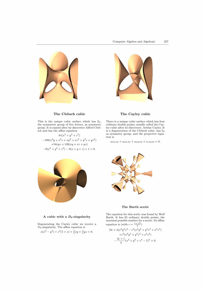
The pictures below were not only chosen to illustrate the beauty of algebraic geomet-ric objects but also because these varieties have had some prominent influence on thedevelopment of algebraic geometry and singularity theory.

The Clebsch cubic itself has been the object of numerous investigations in globalalgebraic geometry, the Cayley and the D4-cubic also, but, moreover, since the D4-cubicdeforms, via the Cayley cubic, to the Clebsch cubic, these first three pictures illustratedeformation theory, an important branch of (computational) algebraic geometry.

The ordinary node, also called A1-singularity (shown as a surface singularity) is themost simple singularity in any dimension. The Barth sextic illustrates a basic, but verydifficult, and still (in general) unsolved problem: to determine the maximum possiblenumber of singularities on a projective variety of given degree. In Section 7.3 we reporton recent progress on this question for plane curves.

Whitney’s umbrella was, at the beginning of stratification theory, an important exam-ple for the two Whitney conditions. We use the umbrella in Section 4.2 to illustrate thatthe algebraic concept of normalization may even lead to a parametrization of a singularvariety, an ultimate goal in many contexts, especially for graphical representations. Ingeneral, however, such a parametrization is not possible, even not locally, if the varietyhas dimension bigger than one. For curve singularities, on the other hand, the normal-ization is always a parametrization. Indeed, computing the normalization of the ideal


The Clebsch cubic

This is the unique cubic surface which has S5,the symmetric group of five letters, as symmetrygroup. It is named after its discoverer Alfred Cleb-sch and has the affine equation

81(x3 + y3 + z3)

−189(x2y + x2z + xy2 + xz2 + y2z + yz2)

+54xyz + 126(xy + xz + yz)

−9(x2 + y2 + z2)− 9(x+ y + z) + 1 = 0.

The Cayley cubic

There is a unique cubic surface which has fourordinary double points, usually called the Cay-ley cubic after its discoverer, Arthur Cayley. Itis a degeneration of the Clebsch cubic, has S4

as symmetry group, and the projective equa-tion is

z0z1z2 + z0z1z3 + z0z2z3 + z1z2z3 = 0.

A cubic with a D4-singularity

Degenerating the Cayley cubic we receive aD4-singularity. The affine equation is

x(x2 − y2) + z2(1 + z) + 25xy + 2

5yz = 0.

The Barth sextic

The equation for this sextic was found by WolfBarth. It has 65 ordinary double points, themaximal possible number for a sextic. Its affine

equation is (with c = 1+√

52

)

(8c+ 4)x2y2z2 − c4(x4y2 + y4z2 + x2z4)

+c2(x2y4 + y2z4 + x4z2)

−2c+ 1

4(x2 + y2 + z2 − 1)2 = 0.

258 G.-M. Greuel

An ordinary node

An ordinary node is the most simple sin-gularity. It has the local equation

x2 + y2 − z2 = 0.

Whitney’s umbrella

Whitney’s umbrella is named after HasslerWhitney who studied it in connection withthe stratification of analytic spaces. It hasthe local equation

y2 − zx2 = 0.

A 5-nodal plane curve of degree 11with equation

−16x2 + 1 048 576y11 − 720 896y9

+180 224y7 − 19712y5 + 880y3 − 11y + 12,

a deformation of A10 : y11 − x2 = 0.

This space curve is given parametricallyby x = t4, y = t3, z = t2, or implicitly by

x− z2 = y2 − z3 = 0.

given by the implicit equations for the space curve in the last picture, we obtain thegiven parametrization. Conversely, the equations are derived from the parametrizationby eliminating t, where elimination of variables is perhaps the most important basicapplication of Grobner bases.

Finally, the 5-nodal plane curve illustrates the global existence problem described inSection 7.2. Moreover, these kind of deformations with the maximal number of nodes


also play a prominent role in the local theory of singularities. For instance, from thisreal picture we can read off the intersection form and, hence, the monodromy of thesingularity A10 by a beautiful theory of A’Campo and Gusein-Zade. We shall present acompletely different, algebraic algorithm to compute the monodromy in Section 6.3.

For more than a hundred years, the connection between algebra and geometry hasturned out to be very fruitful and both merged to one of the leading areas in mathematics:algebraic geometry. The relationship between both disciplines can be characterized bysaying that algebra provides rigour while geometry provides intuition.

In this connection, I place computer algebra on top of rigour, but I should like to stressits limited value if it is used without intuition.

3. Some Problems in Algebraic Geometry

In this section I shall formulate some of the basic questions and problems arising inalgebraic geometry and provide ingredients for certain algorithms. I shall restrict myselfto those algorithms where I am somehow familiar with their implementations and whichhave turned out to be useful in practical applications.

Let me first recall the most basic but also most important applications of Grobnerbases to algebraic constructions (called “Grobner basics” by Sturmfels). Since these canbe found in more or less any textbook dealing with Grobner bases, I just mention them:

• ideal (resp. module) membership problem,• intersection with subrings (elimination of variables),• intersection of ideals (resp. submodules),• Zariski closure of the image of a map,• solvability of polynomial equations,• solving polynomial equations,• radical membership,• quotient of ideals,• saturation of ideals,• kernel of a module homomorphism,• kernel of a ring homomorphism,• algebraic relations between polynomials,• Hilbert polynomial of graded ideals and modules.

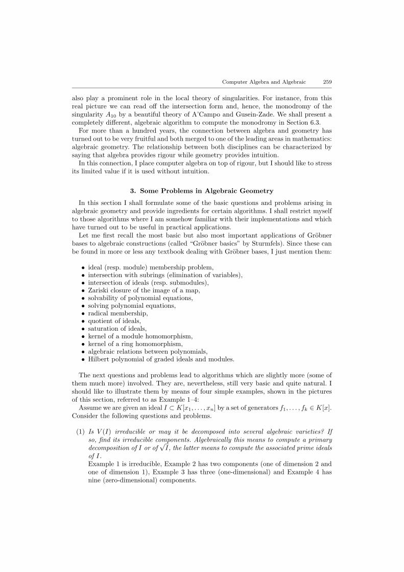
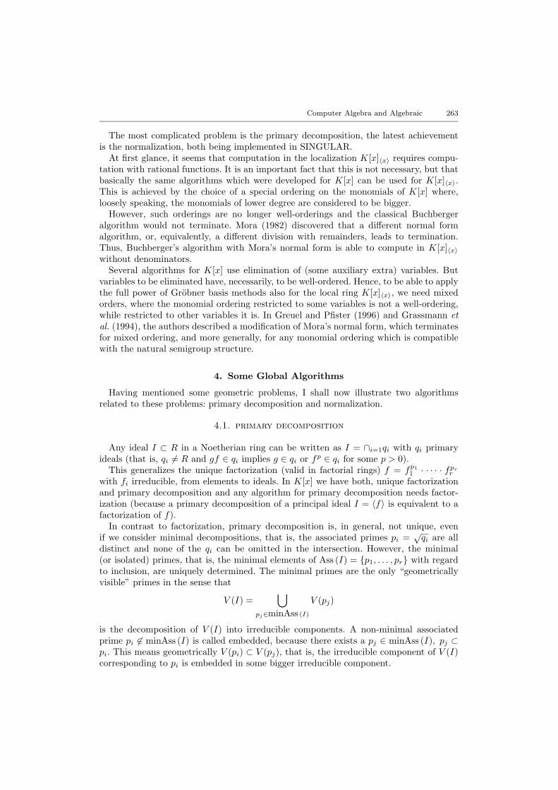
The next questions and problems lead to algorithms which are slightly more (some ofthem much more) involved. They are, nevertheless, still very basic and quite natural. Ishould like to illustrate them by means of four simple examples, shown in the picturesof this section, referred to as Example 1–4:

Assume we are given an ideal I ⊂ K[x1, . . . , xn] by a set of generators f1, . . . , fk ∈ K[x].Consider the following questions and problems.

(1) Is V (I) irreducible or may it be decomposed into several algebraic varieties? Ifso, find its irreducible components. Algebraically this means to compute a primarydecomposition of I or of

√I, the latter means to compute the associated prime ideals

of I.Example 1 is irreducible, Example 2 has two components (one of dimension 2 andone of dimension 1), Example 3 has three (one-dimensional) and Example 4 hasnine (zero-dimensional) components.

260 G.-M. Greuel

(2) Is I a radical ideal (that is, I =√I)? If not, compute its radical

√I.

In Examples 1–3 I is radical while in Example 4√I = 〈y3−y, x3−x〉, which is much

simpler than I. In this example the central point corresponds to V (〈x, y〉2) whichis a fat point, that is, it is a solution of I of multiplicity (= dimK K[x, y]/〈x, y〉2)bigger than 1 (equal to 3). All other points have multiplicity 1, hence the totalnumber of solutions (counted with multiplicity) is 11. This is a typical example ofthe kind Buchberger (resp. Grobner) had in mind at the time of writing his thesis.

(3) A natural question to ask is “how independent are the generators f1, . . . , fk of I?”,that is, we ask for all relations

(r1, . . . , rk) ∈ K[x]k, such that∑

rifi = 0.

These relations form a submodule of K[x]k, which is called the syzygy module off1, . . . , fk and is denoted by syz (I). It is the kernel of the K[x]–linear map

K[x]k −→ K[x]; (r1, . . . , rk) 7−→∑

rifi.

(4) More generally, we may ask for generators of the kernel of a K[x]–linear mapK[x]r −→ K[x]s or, in other words, for solutions of a system of linear equationsover K[x].A direct geometric interpretation of syzygies is not so clear, but there are instanceswhere properties of syzygies have important geometric consequences cf. Schreyer(1986).In Example 1 we have syz (I) = 0, in Example 2, syz (I) = 〈(−y, x)〉 ⊂ K[x]2, inExample 3, syz (I) = 〈(−z, y, 0), (−z, 0, x)〉 ⊂ K[x]3 and in Example 4, syz (I) ⊂K[x]4 is generated by (x,−y, 0, 0), (0, 0, x,−y), (0, x2 − 1,−y2 + 1, 0).

(5) A more geometric question is the following. Let V (I ′) ⊂ V (I) be a subvariety. Howcan we describe V (I)rV (I ′)? Algebraically, this amounts to finding generators forthe ideal quotient

I : I ′ = f ∈ K[x] | fI ′ ⊂ I.

(The same definition applies if I, I ′ are submodules of K[x]k.)Geometrically, V (I : I ′) is the smallest variety containing V (I) r V (I ′) which isthe (Zariski) closure of V (I)r V (I ′).In Example 2 we have 〈xz, yz〉 : 〈x, y〉 = z and in Example 3 〈xy, xz, yz〉 : 〈x, y〉 =〈z, xy〉, which gives, in both cases, equations for the complement of the z-axisx = y = 0. In Example 4 we get I : 〈x, y〉2 = 〈y(y2− 1), x(x2− 1), (x2− 1)(y2− 1)〉which is the zero set of the eight points V (I) with the centre removed.

(6) Geometrically important is the projection of a variety V (I) ⊂ Kn into a linearsubspace Kn−r. Given generators f1, . . . , fk of I, we want to find generators for the(closure of the) image of V (I) in Kn−r = x|x1 = · · · = xr = 0. The image isdefined by the ideal I ∩K[xr+1, . . . , xn] and finding generators for this intersectionis known as eliminating x1, . . . , xr from f1, . . . , fk.Projecting the varieties of Examples 1–3 to the (x, y)-plane is, in the first two cases,surjective and in the third case it gives the two coordinate axes in the (x, y)-plane.This corresponds to the fact that the intersection with K[x, y] of the first two idealsis 0, while the third one is xy.Projecting the nine points of Example 4 to the x–axis we get, by eliminating y,the polynomial x2(x − 1)(x + 1), describing the three image points. From a set


Four examples

Example 1 the hypersurfaceV (x2 + y3 − t2y2)

Example 2 the varietyV (xz, yz)

Example 3 the space curveV (xy, xz, yz)

Example 4 the set of pointsV (y4 − y2, xy3 − xy, x3y − xy, x4 − x2)

theoretical point of view this is nice, however it is not satisfactory if we wish tocount multiplicities. For example, the two border points are the image of threepoints each, hence they should appear with multiplicity three. That this is not thecase can be explained by the fact that elimination computes the annihilator idealof K[x, y]/I considered as K[x]-module (and not the Fitting ideal). This is relatedto the well-known fact that elimination is not compatible with base change.

(7) Another problem is related to the Riemann singularity removable theorem, whichstates that a function on a complex manifold, which is holomorphic and boundedoutside a sub-variety of codimension 1, is actually holomorphic everywhere. This iswell-known for open subsets of C, but in higher dimensions there exists a secondsingularity removable theorem, which states that a function, which is holomorphicoutside a sub-variety of codimension 2 (no assumption on boundedness), is holo-morphic everywhere.For singular complex varieties this is not true in general, but those for which thetwo removable theorems hold are called normal. Moreover, each reduced variety hasa normalization and there is a morphism with finite fibres from the normalizationto the variety, which is an isomorphism outside the singular locus.

262 G.-M. Greuel

The problem is, given a variety V (I) ⊂ Kn, find a normal variety V (J) ⊂ Km anda polynomial map Km −→ Kn inducing the normalization map V (J) −→ V (I).The problem can be reduced to irreducible varieties (but need not be, as we shall see)and then the equivalent algebraic problem is to find the normalization of K[x1, . . . ,xn]/I, that is the integral closure of K[x]/I in the quotient field of K[x]/I andpresent this ring as an affine ring K[y1, . . . , ym]/J for some m and J .For Examples 1–4 it can be shown that the normalization of the first three varietiesis smooth, the last two are the disjoint union of the (smooth) components. Thecorresponding rings are K[x1, x2], K[x1, x2]⊕K[x3], K[x1]⊕K[x2]⊕K[x3]. Thefourth example has no normalization as it is not reduced.A related problem is to find, for a non-normal variety V , an ideal H such thatV (H) is the non-normal locus of V . The normalization algorithm described belowalso solves this problem.In the examples, the non-normal locus is equal to the singular locus.

(8) The significance of singularities appears not only in the normalization problem.The study of singularities is also called local algebraic geometry and belongs to thebasic tasks of algebraic geometry. Nowadays, singularity theory is a whole subjecton its own.A singularity of a variety is a point which has no neighbourhood in which theJacobian matrix of the generators has constant rank.In Example 1 the whole t-axis is singular, in the three other examples only theorigin.One task is to compute generators for the ideal of the singular locus, which is itselfa variety. This is just done by computing sub-determinants of the Jacobian matrix,if there are no components of different dimensions. In general, however, we alsoneed to compute either the equidimensional part and ideal quotients or a primarydecomposition.In Examples 1–4, the singular locus is given by 〈x, y〉, 〈x, y, z〉, 〈x, y, z〉, 〈x, y〉2,respectively.

(9) Studying a variety V (I), I = (f1, . . . , fk), locally at a singular point, say the originof Kn, means studying the ideal IK[x]〈x〉 generated by I in the local ring

K[x]〈x〉 =f

g| f, g ∈ K[x], g 6∈ 〈x1, . . . , xn〉

.

In this local ring the polynomials g with g(0) 6= 0 are units and K[x] is a subringof K[x]〈x〉.Now all the problems we considered above can be formulated for ideals in K[x]〈x〉and modules over K[x]〈x〉 instead of K[x].The geometric problems should be interpreted as properties of the variety in aneighbourhood of the origin, or more generally, the given point.

It should not be surprising that all the above problems have algorithmic and computa-tional solutions, which use, at some place, Grobner basis methods. Moreover, algorithmsfor most of these have been implemented quite efficiently in several computer algebrasystems, such as CoCoA, cf. Capani et al. (1995), Macaulay2, cf. Grayson and Stillmann(1996) and SINGULAR, cf. Greuel et al. (1990–1998), the latter also being able to handle,in addition, local questions systematically.


The most complicated problem is the primary decomposition, the latest achievementis the normalization, both being implemented in SINGULAR.

At first glance, it seems that computation in the localization K[x]〈x〉 requires compu-tation with rational functions. It is an important fact that this is not necessary, but thatbasically the same algorithms which were developed for K[x] can be used for K[x]〈x〉.This is achieved by the choice of a special ordering on the monomials of K[x] where,loosely speaking, the monomials of lower degree are considered to be bigger.

However, such orderings are no longer well-orderings and the classical Buchbergeralgorithm would not terminate. Mora (1982) discovered that a different normal formalgorithm, or, equivalently, a different division with remainders, leads to termination.Thus, Buchberger’s algorithm with Mora’s normal form is able to compute in K[x]〈x〉without denominators.

Several algorithms for K[x] use elimination of (some auxiliary extra) variables. Butvariables to be eliminated have, necessarily, to be well-ordered. Hence, to be able to applythe full power of Grobner basis methods also for the local ring K[x]〈x〉, we need mixedorders, where the monomial ordering restricted to some variables is not a well-ordering,while restricted to other variables it is. In Greuel and Pfister (1996) and Grassmann etal. (1994), the authors described a modification of Mora’s normal form, which terminatesfor mixed ordering, and more generally, for any monomial ordering which is compatiblewith the natural semigroup structure.

4. Some Global Algorithms

Having mentioned some geometric problems, I shall now illustrate two algorithmsrelated to these problems: primary decomposition and normalization.

4.1. primary decomposition

Any ideal I ⊂ R in a Noetherian ring can be written as I = ∩i=1qi with qi primaryideals (that is, qi 6= R and gf ∈ qi implies g ∈ qi or fp ∈ qi for some p > 0).

This generalizes the unique factorization (valid in factorial rings) f = fp11 · · · · · fprr

with fi irreducible, from elements to ideals. In K[x] we have both, unique factorizationand primary decomposition and any algorithm for primary decomposition needs factor-ization (because a primary decomposition of a principal ideal I = 〈f〉 is equivalent to afactorization of f).

In contrast to factorization, primary decomposition is, in general, not unique, evenif we consider minimal decompositions, that is, the associated primes pi =

√qi are all

distinct and none of the qi can be omitted in the intersection. However, the minimal(or isolated) primes, that is, the minimal elements of Ass (I) = p1, . . . , pr with regardto inclusion, are uniquely determined. The minimal primes are the only “geometricallyvisible” primes in the sense that

V (I) =⋃

pj∈minAss (I)

V (pj)

is the decomposition of V (I) into irreducible components. A non-minimal associatedprime pi 6∈ minAss (I) is called embedded, because there exists a pj ∈ minAss (I), pj ⊂pi. This means geometrically V (pi) ⊂ V (pj), that is, the irreducible component of V (I)corresponding to pi is embedded in some bigger irreducible component.

264 G.-M. Greuel

As an example we compute the primary decomposition of the ideal I = 〈x2y3 −x3yz, y2z − xz2〉 in SINGULAR, the output being slightly changed in order to savespace.LIB "primdec.lib"; //calling library for primary decompositionring R = 0,(x,y,z),dp;ideal I = x2y3-x3yz,y2z-xz2;primdecGTZ(I);==> [1]: [1]: [2]: [1]: [3]: [1]:

_[1]=-y2+xz _[1]=z2 _[1]=z[2]: _[2]=y _[2]=x2

_[1]=-y2+xz [2]: [2]:_[1]=z _[1]=z_[2]=y _[2]=x

The result is a list of three pairs of ideals (for each pair, the first ideal is the primarycomponent, the second ideal the corresponding prime component). The second primecomponent [2] : [2] is embedded in the first [1] : [2]. The first primary component [1] : [1]is already prime, the other two are not.

Hence, I = (y2 − xz) ∩ (y, z2) ∩ (x2, z) and we obtain:

V (I) = y2 − xz = 0 ∪ y = z2 = 0(embedded component)

∪ x2 = z = 0

=∪ ∪

Primary decomposition

All known algorithms for primary decompositions in K[x] are quite involved and usemany different sub-algorithms from various parts of computer algebra, in particularGrobner bases, resp. characteristic sets, and multivariate polynomial factorization oversome (algebraic or transcendental) extension of the field K. For an efficient implemen-tation which can treat examples of interest in algebraic geometry, a lot of extra smalladditional algorithms have to be used. In particular one should use “easy” splitting assoon and as often as possible, see Decker et al. (1998).

In SINGULAR the algorithms of Gianni et al. (1988) (which was the first practicaland general primary decomposition algorithm), the recent algorithm of Shimoyama andYokoyama (1996) and some of the homological algebra algorithms for primary decomposi-tion of Eisenbud et al. (1992) have been implemented. For detailed and improved versionsof these algorithms, together with extensive comparisons, see Decker et al. (1998).


Here are some major ingredients for primary decomposition.

(1) Reduction to zero–dimensional primary decomposition (GTZ):maximal independent sets,ideal quotient, saturation, intersection.

(2) Zero-dimensional primary decomposition (GTZ):lexicographical Grobner basis,factorization of multivariate polynomials,generic change of variables,primitive element computation.

Here are some related algorithms.

(1) Computation of the radical:square–free part of univariate polynomials,find (random) regular sequences (EHV).

(2) Computation of the equidimensional part (EHV):Ext–annihilators,ideal quotients, saturation and intersection.

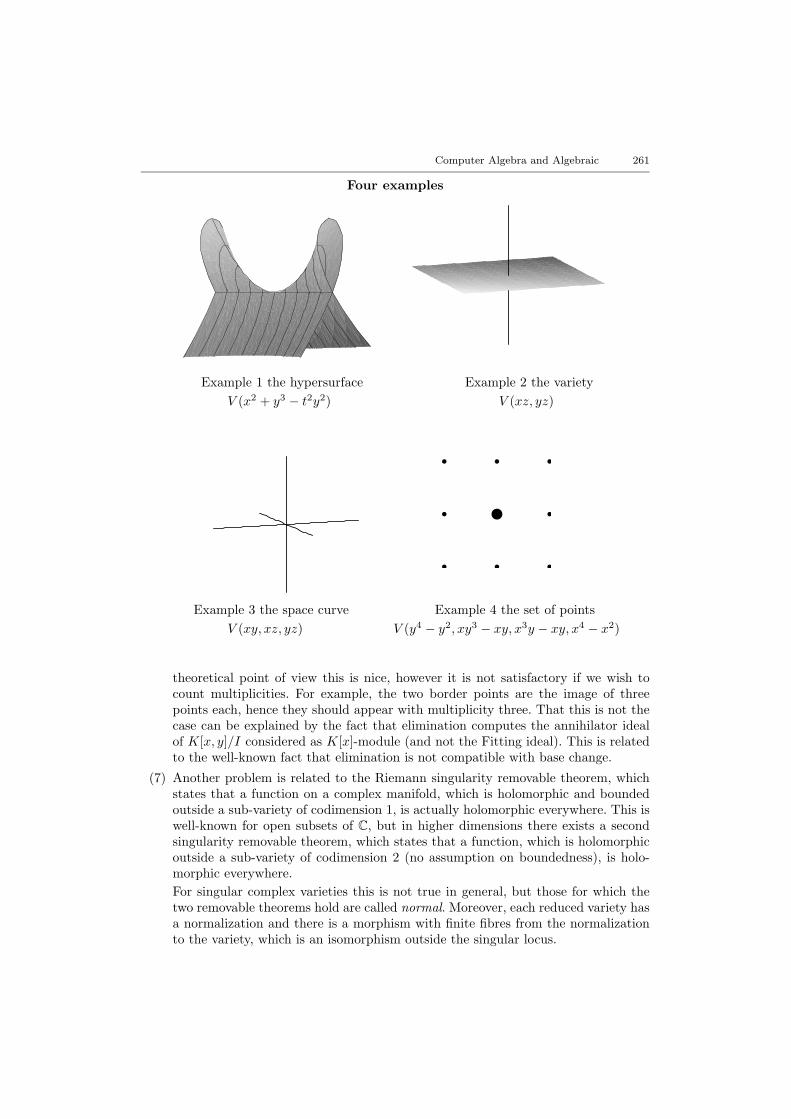
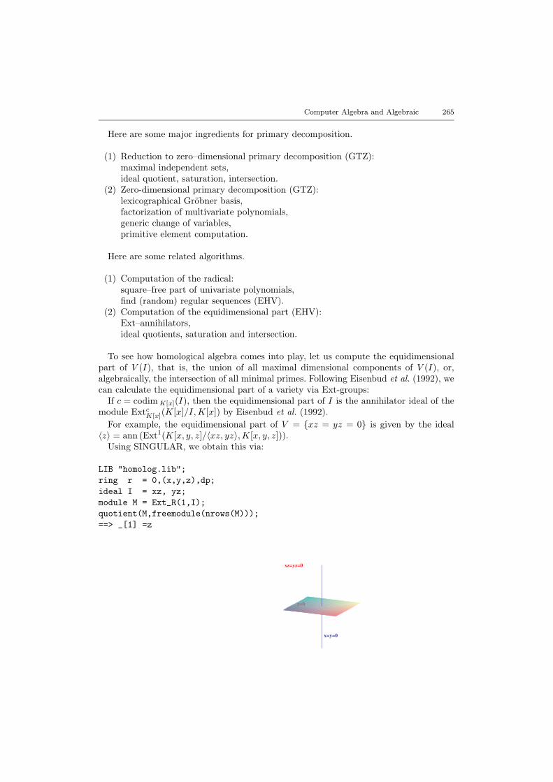
To see how homological algebra comes into play, let us compute the equidimensionalpart of V (I), that is, the union of all maximal dimensional components of V (I), or,algebraically, the intersection of all minimal primes. Following Eisenbud et al. (1992), wecan calculate the equidimensional part of a variety via Ext-groups:

If c = codimK[x](I), then the equidimensional part of I is the annihilator ideal of themodule ExtcK[x](K[x]/I,K[x]) by Eisenbud et al. (1992).

For example, the equidimensional part of V = xz = yz = 0 is given by the ideal〈z〉 = ann (Ext1(K[x, y, z]/〈xz, yz〉,K[x, y, z])).

Using SINGULAR, we obtain this via:

LIB "homolog.lib";ring r = 0,(x,y,z),dp;ideal I = xz, yz;module M = Ext_R(1,I);quotient(M,freemodule(nrows(M)));==> _[1] =z

x=y=0

z=0

xz=yz=0

266 G.-M. Greuel

Note that module M = Ext_R(i,I) computes a presentation matrix of Exti(R/I,R).Hence, identifying a matrix with its column space in the free module of rank equal tothe number of rows, Ext1(R/I,R) = Rn/M with Rn = freemodule(nrows(M)) and,therefore, Ann

(Ext1(R/I,R)

)= M : Rn = quotient(M,freemodule(nrows(M))).

Above, we used the procedure Ext_R(-,-) from homolog.lib. Below we show that theExt-groups can easily be computed directly in a system which offers free resolutions, resp.syzygies, transposition of matrices and presentations of sub-quotients of a free module(modulo in SINGULAR). Indeed, the Ext-annihilator can be computed more directly(and faster) without computing the Ext-group itself:Take a free resolution of R/I :

0←− R/I ←− R←− Rn1 ←− · · · .

Then consider the dual sequence:

0 −→ Hom(R,R) d0

−→ Hom(Rn1 , R) d1

−→ · · · .

This leads to:

Exti(R/I,R) = Ker (di)/Im (di−1) and Ann(Exti(R/I,R)

)= Im (di−1) : Ker (di).

The corresponding SINGULAR commands are:

int i = 1;resolution L = res(I,i+1);module Im = transpose(L[i]);module Ker = syz(transpose(L[i+1]));module ext = modulo(Ker,Im); //the Ext-groupideal ann = quotient(Im,Ker); //the Ext-annihilator

Since the resolution can be computed by iterated syzygy computation, this is a beautifulexample of geometric use of syzygies. However, the algorithm is not at all obvious, butbased on the non-trivial theorem of Eisenbud et al. (1992).

4.2. normalization

Another important algorithm is the normalization of K[x]/I where I is a radical ideal.It can be used as a step in the primary decomposition, as proposed in Eisenbud etal. (1992), but is also of independent interest. Several algorithms have been proposed,especially by Seidenberg (1975), Stolzenberg (1968), Gianni and Trager (1997) and Vas-concelos (1991). It had escaped the computer algebra community, however, that Grauertand Remmert (1971) had given a constructive proof for the ideal of the non-normal lo-cus of a complex space. Within this proof they provide a normality criterion which isessentially an algorithm for computing the normalization, cf. De Jong (1998). Again, tomake the algorithm efficient needed some extra work which is described in Decker et al.(1998). The Grauert–Remmert algorithm is implemented in SINGULAR and seems tobe the only full implementation of the normalization.

Criterion. (Grauert and Remmert, 1971) Let R = K[x]/I with I a radical ideal.Let J be a radical ideal containing a non-zero divisor of R such that V (J) contains thenon-normal locus of V (I). Then R is normal if and only if R = HomR(J, J).


For J we may take any ideal so that V (J) contains the singularities of V (I). Sincenormalization commutes with localization, we obtain

Corollary. Ann(HomR(J, J)/R) is an ideal describing the non-normal locus of V (I).

Now HomR(J, J) is a ring containing R and if R $ HomR(J, J) = R1 we can continuewith R1 instead of R and obtain an increasing sequence of rings R ⊂ R1 ⊂ R2 ⊂ . . . .

After finitely many steps the sequence becomes stationary (because the normalizationof R = K[x]/I is finite over R) and we reach the normalization of R by the criterion ofGrauert and Remmert.

Ingredients for the normalization (which is a highly recursive algorithm):

(1) computation of the ideal J of the singular locus of the ideal I,(2) computation of a non-zero divisor for J ,(3) ring structure on Hom(J, J),(4) syzygies, normal forms, ideal quotient.

SINGULAR commands for computation of the normalization:LIB "normal.lib";ring S = 0,(x,y,z),dp;ideal I = y2-x2z;list nor = normal(I);def R = nor[1];setring R;normap;==> normap[1]=T(1)==> normap[2]=T(1)*T(2)==> normap[3]=T(2)^2

(s, t) 7→ (s, st, t2)

In the preceding picture, R, the normalization of S, is just the polynomial ring in twovariables T (1) and T (2). (The “handle” of Whitney’s umbrella is invisible in the para-metric picture since it requires an imaginary parameter t.)

In several cases the normalization of a variety is smooth (for example, the normalizationof the discriminant of a versal deformation of an isolated hypersurface singularity) some-times even an affine space. In this case, the normalization map provides a parametrizationof the variety. This is the case for Whitney’s umbrella: V = y2 − zx2 = 0.

5. Singularities and Standard Bases

A (complex) singularity is, by definition, nothing but a complex analytic germ (V, 0)together with its analytic local ring R = Cx/I, where Cx is the convergent powerseries ring in x = x1, . . . , xn. For an arbitrary field K let R = K[[x]]/I for some ideal Iin the formal power series ring K[[x]]. We call (V, 0) = (SpecR,m) or just R a singularity(m denotes the maximal ideal of the local ring R) and write K〈x〉 for the convergent andfor the formal power series ring if the statements hold for both.

If I ⊂ K[x] is an ideal with I ⊂ 〈x〉 = 〈x1, . . . , xn〉 then the singularity of V (I) at0 ∈ Kn is, using the above notation, K〈x〉/I ·K〈x〉. However, we may also consider thelocal ring K[x]〈x〉/I ·K[x]〈x〉 with K[x]〈x〉 the localization of K[x] at 〈x〉, as the singularity

268 G.-M. Greuel

of V (I) at 0. Geometrically, for K = C, the difference is the following: Cx/ICxdescribes the variety V (I) in an arbitrary small neighbourhood of 0 in the Euclideantopology while C[x]〈x〉/IC[x]〈x〉 describes V (I) in an arbitrary small neighbourhood of 0in the (much coarser) Zariski topology.

At the moment, we can compute efficiently only in K[x]〈x〉 as we shall explain below.In many cases of interest, we are happy since invariants of V (I) at 0 can be computedin K[x]〈x〉 as well as in K〈x〉. There are, however, others (such as factorization), whichare completely different in both rings.

Isolated singularities

Non–isolated singularities

A1 : x2 − y2 + z2 = 0 D4 : z3 − zx2 + y2 = 0

A∞ : x2 − y2 = 0 D∞ : y2 − zx2 = 0

(V, 0) is called non-singular or regular or smooth if K〈x〉/I is isomorphic (as local ring)to a power series ring K〈y1, . . . , yd〉, or if K[x]〈x〉/I is a regular local ring.

By the implicit function theorem, or by the Jacobian criterion, this is equivalent tothe fact that I has a system of generators g1, . . . , gn−d such that the Jacobian matrix ofg1, . . . , gn−d has rank n − d in some neighbourhood of 0. (V, 0) is called an isolatedsingularity if there is a neighbourhood W of 0 such that W ∩ (V r 0) is regulareverywhere.

In order to compute with singularities, we need the notion of standard basis which isa generalization of the notion of the Grobner basis, cf. Greuel and Pfister (1996, 1998).

A monomial ordering is a total order on the set of monomials xα|α ∈ Nn satisfying

xα > xβ ⇒ xα+γ > xβ+γ for all α, β, γ ∈ Nn.


We call a monomial ordering > global (resp. local, resp. mixed) if xi > 1 for all i (resp.xi < 1 for all i, resp. if there exist i, j so that xi < 1 and xj > 1). This notion is justifiedby the associated ring to be defined below. Note that > is global if and only if > is awell-ordering (which is usually assumed).

Any f ∈ K[x] r 0 can be written uniquely as f = cxα + f ′, with c ∈ K r 0 andα > α′ for any non-zero term c′xα

′of f ′. We set lm(f) = xα, the leading monomial of f

and lc (f) = c, the leading coefficient of f .For a subset G ⊂ K[x] we define the leading ideal of G as

L(G) = 〈 lm(g) | g ∈ Gr 0〉K[x],

the ideal generated by the leading monomials in Gr 0.So far, the general case is not different to the case of a well-ordering. However, the

following definition provides something new for non-global orderings:For a monomial ordering > define the multiplicatively closed set

S> := u ∈ K[x]r 0 | lm (u) = 1and the K–algebra

R := LocK[x] := S−1> K[x] =

f

u| f ∈ K[x], u ∈ S>

,

the localization (ring of fractions) of K[x] with respect to S>. We call LocK[x] also thering associated to K[x] and >.

Note that K[x] ⊂ LocK[x] ⊂ K[x]〈x〉 and LocK[x] = K[x] if and only if > is globaland LocK[x] = K[x]〈x〉 if and only if > is local (which justifies the names).

Let > be a fixed monomial ordering. In order to have a short notation, I write

R := LocK[x] = S−1> K[x]

to denote the localization of K[x] with respect to >.Let I ⊂ R be an ideal. A finite set G ⊂ I is called a standard basis of I if and only if

L(G) = L(I), that is, for any f ∈ I r 0 there exists a g ∈ G satisfying lm (g)|lm (f).If the ordering is a well-ordering, then a standard basis G is called a Grobner basis. In

this case R = K[x] and, hence, G ⊂ I ⊂ K[x].Standard bases can be computed in the same way as Grobner bases except that we

need a different normal form. This was first noticed by Mora (1982) for local orderings(called tangent cone orderings by Mora) and, in general, by Greuel and Pfister (1996)and Grassmann et al. (1994).

Let G denote the set of all finite and ordered subsets G ⊂ R. A map

NF : R× G → R, (f,G) 7→ NF (f |G),

is called a normal form on R if, for all f and G,

(i) NF (f |G) 6= 0⇒ lm(NF (f |G)

)6∈ L(G),

(ii) f −NF (f |G) ∈ 〈G〉R, the ideal in R generated by G.

NF is called a weak normal form if, instead of (ii), only the following condition (ii′)holds:

(ii′) for each f ∈ R and each G ∈ G there exists a unit u ∈ R, so that uf −NF (f |G) ∈〈G〉R.

270 G.-M. Greuel

Moreover, we need (in particular for computing syzygies) (weak) normal forms withstandard representation: if G = g1, . . . , gk, we can write

f −NF (f |G) =k∑i=1

aigi, ai ∈ R,

such that lm(f−NF (f |G)

)≥ lm (aigi) for all i, that is, no cancellation of bigger leading

terms occurs among the aigi.Indeed, if f and G consist of polynomials, we can compute, in finitely many steps, weak

normal forms with standard representation such that u and NF (f |G) are polynomialsand, hence, compute polynomial standard bases which enjoy most of the properties ofGrobner bases.

Once we have a weak normal form with standard representation, the general standardbasis algorithm may be formalized as follows:

Standardbasis(G,NF) [arbitrary monomial ordering]Input: G a finite and ordered set of polynomials, NF a weak normal form with standardrepresentation.Output: S a finite set of polynomials which is a standard basis of 〈G〉R.– S = G;– P = (f, g) | f, g ∈ S;– while (P 6= ∅)

choose (f, g) ∈ P ;P = P r (f, g);h = NF (spoly(f, g) | S);if (h 6= 0)

P = P ∪ (h, f) | f ∈ S;S = S ∪ h;

– return S;Here spoly(f, g) = xγ−αf − lc(f)

lc(g)xγ−βg denotes the s-polynomial of f and g where

xα = lm (f), xβ = lm (g), γ = lcm(α, β).The algorithm terminates by Dickson’s lemma or by the noetherian property of the

polynomial ring (and since NF terminates). It is correct by Buchberger’s criterion, whichgeneralizes to non-well-orderings.

If we use Buchberger’s normal form below, in the case of a well-ordering, Standard-

basis is just Buchberger’s algorithm:

NFBuchberger(f,G) [ well-ordering ]Input: G a finite ordered set of polynomials, f a polynomial.Output: h a normal form of f with respect to G with standard representation.– h = f ;– while (h 6= 0 and exist g ∈ G so that lm (g) | lm (h))

choose any such g;h = spoly(h, g);

– return h;For an algorithm to compute a weak normal form in the case of an arbitrary ordering,

we refer to Greuel and Pfister (1996).To illustrate the difference between local and global orderings, we compute the dimen-

sion of a variety at a point and the (global) dimension of the variety.


The dimension of the singularity (V, 0), or the dimension of V at 0, is, by definition, theKrull dimension of the analytic local ring OV,0 = K〈x〉/I, which is the same as the Krulldimension of the algebraic local ring K[x]〈x〉/I in case I = 〈f1, . . . , fk〉 is generated bypolynomials, which follows easily from the theory of dimensions by the Hilbert–Samuelseries.

Using this fact, we can compute dim(V, 0) by computing a standard basis of the ideal〈f1, . . . , fk〉 generated in LocK[x] with respect to any local monomial ordering on K[x].The dimension is equal to the dimension of the corresponding monomial ideal (which isa combinatorial problem).

For example, the dimension of the affine variety V = V (yx − y, zx − z) is 2 but thedimension of the singularity (V, 0) (that is, the dimension of V at the point 0) is 1:

0

V : y(x− 1) = z(x− 1) = 0,dim(V, 0) = 1, dimV = 2

Using SINGULAR we compute first the global dimension with the degree reverselexicographical ordering denoted by dp and then the local dimension at 0 using thenegative degree reverse lexicographical ordering denoted by ds. Note that in the localring K[x, y]〈x,y〉 (represented by the ordering ds) x− 1 is a unit.

ring R = 0,(x,y,z),dp; //global ringideal i = yx-y,zx-z;ideal si = groebner(i);si;==> si[1]=xz-z, //leading ideal of i is <xz,xy>==> si[2]=xy-ydim(si);==> 2 //global dimension = dim R/<xz,xy>

ring r = 0,(x,y,z),ds; //local ringideal i = yx-y,zx-z;ideal si = groebner(i);si;==> si[1]=y //leading ideal of i is <y,z>==> si[2]=zdim(si);==> 1 //local dimension = dim r/<y,z>

272 G.-M. Greuel

6. Some Local Algorithms

I describe here three algorithms which use, in an essential way, standard bases for localrings: classification of singularities, deformations and the monodromy.

6.1. classification of singularities

In the late sixties, V. I. Arnold started a tremendous work–the classification of hy-persurface singularities up to right equivalence. Here f and g ∈ K〈x1, . . . , xn〉 are calledright equivalent if they coincide up to analytic coordinate transformation, that is, ifthere exists a local K–algebra automorphism ϕ of K〈x〉 such that f = ϕ(g). His workculminated in impressive lists of normal forms of singularities and, moreover, in a deter-minator for singularities which allows the determination of the normal form for a givenpower series ([AGV, II.16]). This work of Arnold has found numerous applications invarious areas of mathematics, including singularity theory, algebraic geometry, differen-tial geometry, differential equations, Lie group theory and theoretical physics. The workof Arnold was continued by C. T. C. Wall and others, cf. Wall (1983) and Greuel andKroning (1990).

Most prominent is the list of ADE or simple or Kleinian singularities, which have ap-peared in surprisingly different areas of mathematics, and still today, new connectionsof these singularities to other areas are being discovered (for a survey see Greuel, 1992).Here is the list of ADE singularities (the names come from their relation to the simpleLie groups of type A, D and E).

Ak : xk+11 + x2

2 + x23 + · · ·+ x2

n, k ≥ 1Dk : x1(xk−2

1 + x22) + x2

3 + · · ·+ x2n, k ≥ 4

E6 : x41 + x3

2 + x23 + · · ·+ x2

n,

E7 : x2(x31 + x2

2) + x23 + · · ·+ x2

n,

E8 : x51 + x3

2 + x23 + · · ·+ x2

n.

A3-singularity D6-singularity E7-singularity

Arnold introduced the concept of “modality”, related to Riemann’s idea of moduli, intosingularity theory and classified all singularities of modality ≤ 2 (and also of Milnor


number≤ 16). The ADE singularities are just the singularities of modality 0. Singularitiesof modality 1 are the three parabolic singularities:

E6 = P8 = T333 : x3 + y3 + z3 + axyz, a3 + 27 6= 0,E7 = Xg = T244 : x4 + y4 + ax2y2, a2 6= 4,

E8 = J10 = T236 : x3 + y5 + ax2y2, 4a3 + 27 6= 0,

the three-indexed series of hyperbolic singularities

Tpqr : xp + yq + zr + axyz, a 6= 0,1p

+1q

+1r< 1

and 14 exceptional families, cf. Arnold et al. (1985).The proof of Arnold for his determinator is, to a great part constructive, and has been

partly implemented in SINGULAR, cf. Kruger (1997). Although the whole theory andthe proofs deal with power series, everything can be reduced to polynomial computationsince we deal with isolated singularities, which are finitely determined. That is, for anisolated singularity f , there exists an integer k such that f and g are right equivalent iftheir Taylor expansion coincides up to order k. Therefore, knowing the determinacy k off , we can replace f by its Taylor polynomial up to order k.

The determinacy can be estimated as the minimal k such that

mk+1 ⊂ m2 jacob(f)

where m ⊂ K〈x1, . . . , xn〉 is the maximal ideal and jacob(f) = 〈∂f/∂x1, . . . , ∂f/∂xn〉.Hence, this k can be computed by computing a standard basis of m2 jacob(f) and normalforms of mi with respect to this standard basis for increasing i, using a local monomialordering. However, there is a much faster way to compute the determinacy directly froma standard basis of m2 jacob(f), which is basically the “highest corner” described inGreuel and Pfister (1996).

An important initial step in Arnold’s classification is the generalized Morse lemma,or splitting lemma, which says that f ϕ(x1, . . . , xn) = x2

1 + · · · + x2r + g(xr+1, . . . , xn)

for some analytic coordinate change ϕ and some power series g ∈ m3 if the rank of theHessian matrix of f at 0 is r.

The determinacy allows the computation of ϕ up to sufficiently high order and apolynomial g as in the theorem. This has been implemented in SINGULAR and is acornerstone in classifying hypersurface singularities.

In the following example we use SINGULAR to get the singularity T5,7,11 from adatabase A−L (“Arnold’s list”), make some coordinate change and determine then thenormal form of the complicated polynomial after coordinate change.

LIB "classify.lib";ring r = 0,(x,y,z),ds;poly f = A_L("T[5,7,11]");f;==> xyz+x5+y7+z11map phi = r, x+z,y-y2,z-x;poly g = phi(f);g;==> -x2y+yz2+x2y2-y2z2+x5+5x4z+10x3z2+10x2z3+5xz4+z5+y7-7y8+21y9-35y10==> -x11+35y11+11x10z-55x9z2+165x8z3-330x7z4+462x6z5-462x5z6+330x4z7

274 G.-M. Greuel

==> -165x3z8+55x2z9-11xz10+z11-21y12+7y13-y14classify(g);==> The singularity ... is R-equivalent to T[p,q,r]=T[5,7,11]

Ingredients for the classification of singularities:

(1) standard bases for local and global orderings,(2) computation of invariants (Milnor number, determinacy, . . . ),(3) generalized Morse lemma,(4) syzygies for local orderings.

Beyond classification by normal forms, the construction of moduli spaces for singu-larities, for varieties or for vector bundles is a pretentious goal, theoretically as well ascomputational. First steps towards this goal for singularities have been undertaken inBayer (2000) and Fruhbis-Kruger (2000).

6.2. deformations

Consider a singularity (V, 0) given by the power series f1, . . . , fk ∈ K〈x1, . . . , xn〉. Theidea of deformation theory is to perturb the defining functions, that is to consider thepower series F1(t, x), . . . , Fk(t, x) with Fi(0, x) = fi(x), where t ∈ S may be consideredas a small parameter of a parameter space S (containing 0).

For t ∈ S the power series fi,t(x) = Fi(t, x) define a singularity Vt, which is a pertur-bation of V = V0 for t 6= 0 close to 0. It may be hoped that Vt is simpler than V0 butstill contains enough information about V0. For this hope to be fulfilled, it is, however,necessary to restrict the possible perturbations of the equations to flat perturbations,which are called deformations.

Grothendieck’s criterion of flatness states that the perturbation given by the Fi is flatif and only if any relation between the fi, say∑

ri(x)fi(x) = 0,

lifts to a relation ∑Ri(t, x)Fi(t, x) = 0,

with Ri(x, 0) = ri(x). Equivalently, for any generator (r1, . . . , rk) of syz (f1, . . . , fk) thereexists an element (R1, . . . , Rk) ∈ syz (F1, . . . , Fk) satisfying Ri(0, x) = ri(x). Hence,syzygies with respect to local orderings come into play.

There exists the notion of a semi-universal deformation of (V, 0) which contains essen-tially all information about all deformations of (V, 0).

For an isolated hypersurface singularity f(x1, . . . , xn) the semi-universal deformationis given by

F (t, x) = f(x) +τ∑j=1

tjgj(x),

where 1 =: g1, g2, . . . , gτ represent a K–basis of the Tjurina algebra

K〈x〉/〈f, ∂f/∂x1, . . . , ∂f/∂xn〉,


τ = dimK K〈x〉/〈f, ∂f/∂x1, . . . , ∂f/∂xn〉 being the Tjurina number.To compute g1, . . . , gτ we only need to compute a standard basis of the ideal 〈f, ∂f∂x1

, . . . ,∂f∂xn〉 with respect to a local ordering and then compute a basis of K[x] modulo the leading

monomials of the standard basis. For complete intersections we have similar formulas.

Deformation of E7 in 4A1

For non-hypersurface singularities, the semi-universal deformation is much more com-plicated and up to now no finite algorithm is known in general. However, there exists analgorithm to compute this deformation up to arbitrary high order cf. Laudal (1979) andMartin (1998), which is implemented in SINGULAR.

As an example we calculate the base space of the semi-universal deformation of thenormal surface singularity, being the cone over the rational normal curve C of degree 4,parametrized by t 7→ (t, t2, t3, t4).

Homogeneous equations for the cone over C are given by the 2×2-minors of the matrix:

m =(x y z u

y z u v

)∈ Mat 2×4(K[x, y, z, u, v]).

SINGULAR commands for computing the semi-universal deformation:

LIB "deform.lib";ring r = 0,(x,y,z,u,v),ds;matrix m[2][4] = x,y,z,u,y,z,u,v;ideal f = minor(m,2);versal(f);setring Px;Fs;==> Fs[1,1]=-u2+zv+Bu+Dv==> Fs[1,2]=-zu+yv-Au+Du==> Fs[1,3]=-yu+xv+Cu+Dz==> Fs[1,4]=z2-yu+Az+By==> Fs[1,5]=yz-xu+Bx-Cz

276 G.-M. Greuel

==> Fs[1,6]=-y2+xz+Ax+CyJs;==> Js[1,1]=BD==> Js[1,2]=AD-D2==> Js[1,3]=-CD

D=0

A-D=0

B=C=0

The ideal Js = 〈BD,AD − D2,−CD〉 ⊂ K[A,B,C,D] defines the required basespace which consists of a three-dimensional component (D = 0) and a transversal one-dimensional component (B = C = A − D = 0). This was the first example, found byPinkham, of a base space of a normal surface having several components of differentdimensions.

The full versal deformation is given by the map (Fs and Js as above)

K[[A,B,C,D]]/Js −→ K[[A,B,C,D, x, y, z, u, v]]/Js + Fs.

Although, in general, the equations for the versal deformation are the formal powerseries, in many cases of interest (as in the example above) the algorithm terminates andthe resulting ideals are polynomial.

Ingredients for the semi-universal deformation algorithm:

(1) Computation of standard bases, normal forms and resolutions for local orderings,(2) computation of Ext-groups (cf. 4.1) for computing infinitesimal deformations and

obstructions,(3) computation of Massey products for determining obstructions to lift, recursively,

infinitesimal deformations of a given order to higher order,(4) one of the main difficulties in point 3 is the necessity to compute a completely

reduced normal form with respect to a local ordering. In general, such a normalform exists only as a formal power series. In the present situation, however, thereduction has to be carried out only for a subset of the variables in a fixed degreeand, hence, the complete reduction is finite.


6.3. the monodromy

Let f ∈ Cx1, . . . , xn be a convergent power series (in practice a polynomial) withisolated singularity at 0 and µ = dimC Cx/〈fx1 , . . . , fxn〉 the Milnor number of f .

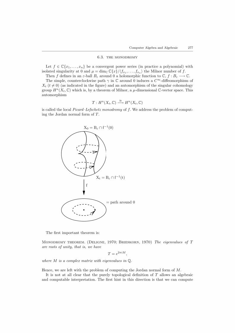
Then f defines in an ε-ball Bε around 0 a holomorphic function to C, f : Bε −→ C.The simple, counterclockwise path γ in C around 0 induces a C∞-diffeomorphism of

Xt (t 6= 0) (as indicated in the figure) and an automorphism of the singular cohomologygroup Hn(Xt,C) which is, by a theorem of Milnor, a µ-dimensional C-vector space. Thisautomorphism

T : Hn(Xt,C)∼=−→ Hn(Xt,C)

is called the local Picard–Lefschetz monodromy of f . We address the problem of comput-ing the Jordan normal form of T .

X0 = Bε ∩ f−1(0)

Xt = Bε ∩ f−1(t)

f

= path around 0

The first important theorem is:

Monodromy theorem. (Deligne, 1970; Brieskorn, 1970) The eigenvalues of Tare roots of unity, that is, we have

T = e2πiM ,

where M is a complex matrix with eigenvalues in Q.

Hence, we are left with the problem of computing the Jordan normal form of M .It is not at all clear that the purely topological definition of T allows an algebraic

and computable interpretation. The first hint in this direction is that we can compute

278 G.-M. Greuel

dimCHn(Xt,C), according to Milnor’s theorem, algebraically by the formula for µ givenabove.

Since Xt is a complex Stein manifold, its complex cohomology can be computed, viathe holomorphic de Rham theorem, with holomorphic differential forms, which is thestarting point for computing the monodromy.

To cut a long story short, we just mention, cf. Brieskorn (1970) and Greuel (1975) that

H ′ = Ωn/df ∧ Ωn−1 + dΩn−1,

H ′′ = Ωn+1/df ∧ dΩn−1

are free Ct–modules (via f∗ : Ct −→ Cf ⊂ Cx) of rank equal to µ. Here (Ω•, d)denotes the complex of holomorphic differential forms in (Cn, 0). H ′ and H ′′ are calledBrieskorn lattices.

We define the local Gauss–Manin connection of f as

5 : df ∧H ′ = df ∧ Ωn/df ∧ dΩn−1 −→ H ′′,

5[df ∧ ω] = [dω].

Note that 5(df ∧H ′) 6⊂ df ∧H ′, that is, 5 has a pole at 0. Tensoring with C (t), thequotient field of Ct, we can extend 5 to a meromorphic connection

5 : H ′′ ⊗Ct

C(t) −→ H ′′ ⊗Ct

C(t)

(since df ∧H ′ ⊗ C(t) = H ′′ ⊗ C(t)) using the Leibnitz rule 5(ωy) = 5(ω)y + ωdy/dt.With respect to a basis ω1, . . . , ωµ of H ′′ we have 5(ωi) =

∑j

ajiωj and, for any

ω =∑i

ωiyi, 5(ω) =∑i,j

ajiyi +∑i

ωidyi/dt. Hence, the kernel of 5, together with a

basis of H ′′, is the same as the solutions of the system of rank µ of ordinary differentialequations

dy

dt= −Ay, A = (aij) ∈ Mat

(µ× µ,C(t)

)in a neighbourhood of 0 in C. The connection matrix, A =

∑i≥−p

Aiti, Ai ∈ Mat (µ×µ,C),

has a pole at t = 0 and is holomorphic for t 6= 0. If φt = (φ1, . . . , φµ) is a fundamentalsystem of solutions at a point t 6= 0, then the analytic continuation of φt along the pathγ transforms φt into another fundamental system φ′t which satisfies φ′t = T5φt for somematrix T5 ∈ GL(µ,C).

Fundamental fact. (Brieskorn, 1970) The Picard–Lefschetz monodromy T coin-cides with the monodromy T5 of the Gauss–Manin connection.

Brieskorn (1970) used this fact to describe the essential steps for an algorithm tocompute the characteristic polynomial of T . Results of Gerard and Levelt allowed theextension of this algorithm to compute the Jordan normal form of T , cf. (1973). An earlyimplementation by Nacken in Maple was not very efficient. Recently, Schulze (1999)implemented an improved version in SINGULAR which is able to compute interestingexamples.

The algorithm uses another basic theorem, the


Regularity theorem. (Brieskorn, 1970) The Gauss–Manin connection has a reg-ular singular point at 0, that is, there exists a basis of some lattice in H ′′ ⊗ C(t) suchthat the connection matrix A has pole of order 1.

Basically, if A = A−1t−1 + A0 + A1t + · · · has a simple pole, then T = e2πiA−1 is the

monodromy (this holds if the eigenvalues of A−1 do not differ by integers which can beachieved algorithmically).SINGULAR example:

LIB "mondromy.lib";ring R = 0,(x,y),ds;poly f = x2y2+x6+y6; //example of A’Campo (monodromy is not

diagonalisable)matrix M = monodromy(f);print(jordanform(M));==> 1/2,1, 0, 0, 0, 0, 0,0,0,0, 0, 0, 0,==> 0, 1/2,0, 0, 0, 0, 0,0,0,0, 0, 0, 0,==> 0, 0, 2/3,0, 0, 0, 0,0,0,0, 0, 0, 0,==> 0, 0, 0, 2/3,0, 0, 0,0,0,0, 0, 0, 0,==> 0, 0, 0, 0, 5/6,0, 0,0,0,0, 0, 0, 0,==> 0, 0, 0, 0, 0, 5/6,0,0,0,0, 0, 0, 0,==> 0, 0, 0, 0, 0, 0, 1,0,0,0, 0, 0, 0,==> 0, 0, 0, 0, 0, 0, 0,1,0,0, 0, 0, 0,==> 0, 0, 0, 0, 0, 0, 0,0,1,0, 0, 0, 0,==> 0, 0, 0, 0, 0, 0, 0,0,0,7/6,0, 0, 0,==> 0, 0, 0, 0, 0, 0, 0,0,0,0, 7/6,0, 0,==> 0, 0, 0, 0, 0, 0, 0,0,0,0, 0, 4/3,0,==> 0, 0, 0, 0, 0, 0, 0,0,0,0, 0, 0, 4/3

Ingredients for the monodromy algorithm:

(1) computation of standard bases and normal forms for local orderings,

(2) computation of Milnor number,

(3) Taylor expansion of units in K[x]〈x〉 up to sufficiently high order,

(4) computation of the connection matrix on increasing lattices in H ′′ ⊗ C(t) up tosufficiently high order (until saturation) by linear algebra over Q,

(5) computation of the transformation matrix to a simple pole by linear algebra over Q,

(6) factorization of univariate polynomials (for Jordan normal form).

The most expensive parts are certain normal form computations for a local orderingand the linear algebra part because here one has to deal iteratively with matrices withseveral thousand rows and columns. It turned out that the SINGULAR implementation ofmodules (considered as sparse matrices) and the Buchberger inter-reduction is sufficientlyefficient (though not the best possible) for such tasks.

280 G.-M. Greuel

7. Computer Algebra Solutions to Singularity Problems

We present three examples which demonstrate, in a somewhat typical way, the use ofcomputer algebra as stated in the preface:

(1) producing counter examples,(2) providing evidence and prompting proofs for new theorems,(3) constructing interesting explicit examples.

7.1. exactness of the Poincaree complex

The first application is a counterexample to a conjectured generalization of a theoremof Saito (1971) which says that, for an isolated hypersurface singularity, the exactnessof the Poincare complex implies that the defining polynomial is, after some analyticcoordinate change, weighted homogeneous.

Theorem. (Saito, 1971) If f : Cn+1 −→ C has an isolated singularity at 0, then thefollowing are equivalent:

(1) X = f−1(0) is weighted homogeneous for a suitable choice of coordinates.(2) µ = τ where µ = dimC Cx/

(∂f∂xi

)is the Milnor number and

τ = dimC Cx/(f, ∂f∂xi

)the Tjurina number.

(3) The holomorphic Poincare complex

0 −→ C −→ OXd−→ Ω1

Xd−→ Ω2

X −→ · · · −→ ΩnX −→ 0

is exact.

A natural problem is whether the theorem holds also for complete intersections X =f−1(0) with f = (f1, . . . , fk) : Cn+k −→ C

k. Again we have a Milnor number µ and aTjurina number τ ,

µ =k∑i=1

(−1)i−1 dimC Cx

/(f1, . . . , fi−1,

∣∣∣∣∣ ∂(f1, . . . , fi)∂(xj1 , . . . , xji)

∣∣∣∣∣)

τ = dimCCxk/(f1, . . . , fk)Cxk +Df(Cxn+k).

Theoretical reduction. (Greuel et al., 1985) If X is a complete intersection ofdimension 1, then (1) ⇔ (2) ⇒ (3).If k = 2, then (3) ⇒ (2) if µ = dimC Ω2

X − dimC Ω3X and if f1, f2 are weighted homoge-

neous.

Pfister and Schonemann (1989) showed that (3) ⇒ (2) does not hold in general:

f1 = xy + z`−1, f2 = xz + yk−1 + yz2 (4 ≤ ` ≤ k, k ≥ 5)

is a counterexample.The proof uses an implementation of the standard basis algorithm in a forerunner of

SINGULAR and goes as follows:


(1) compute µ,dimC Ω2X ,dimCΩ3

X to show that Ω•X is exact,(2) compute τ .

One obtains µ = τ + 1, that is, X is not weighted homogeneous.

To do this we must be able to compute standard bases of modules over local rings.The counterexample was found through a computer search in a list of singularities

classified by Wall (1983).

7.2. Zariski’s multiplicity conjecture

The attempt to find a counterexample to Zariski’s multiplicity conjecture—which saysthat the multiplicity (lowest degree) of a power series is an invariant of the embed-ded topological type—after many experiments and computations, finally led to a partialproof of this conjecture. For this, an extremely fast standard basis computation for zero-dimensional ideals in a local ring was necessary.

The following question was posed by Zariski (1971) in his retiring address to the AMSin 1971.

Let f =∑cαx

α ∈ Cx1, . . . , xn, f(0) = 0, be a hypersurface singularity, and letmult (f) := min

|α|∣∣ cα 6= 0

be the multiplicity.

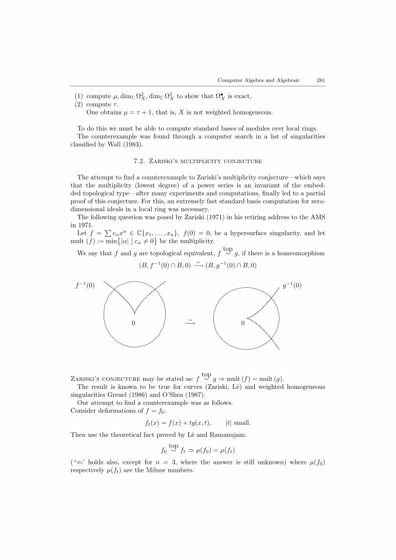
We say that f and g are topological equivalent, ftop∼ g, if there is a homeomorphism

(B, f−1(0) ∩B, 0) ∼−→ (B, g−1(0) ∩B, 0)

f−1(0)

0 ∼−→ 0

g−1(0)

Zariski’s conjecture may be stated as: ftop∼ g ⇒ mult (f) = mult (g).

The result is known to be true for curves (Zariski, Le) and weighted homogeneoussingularities Greuel (1986) and O’Shea (1987).

Our attempt to find a counterexample was as follows.Consider deformations of f = f0:

ft(x) = f(x) + tg(x, t), |t| small.

Then use the theoretical fact proved by Le and Ramanujam:

f0top∼ ft ⇒ µ(f0) = µ(ft)

(“⇐’ holds also, except for n = 3, where the answer is still unknown) where µ(f0)respectively µ(ft) are the Milnor numbers.

282 G.-M. Greuel

We tried to construct a deformation ft of f0 where the multiplicity mult (ft) drops butthe Milnor number µ(ft) is constant.

Our candidates (a, b, c ∈ N) came from a heuristical investigation of the Newton dia-gram, one being the following series:

ft = xa + yb + z3c + xc+2yc−1 + xc−1yc−1z3 + xc−2yc(y2 + tx)2, a, b, c ∈ N.

Obviously, the multiplicity drops. Computing µ with SINGULAR, we obtain for (a, b, c) =(37, 27, 6): µ(f0) = 4840, µ(ft) = 4834, thus f0 and ft are (unfortunately) not topologi-cally equivalent.

Since the Milnor numbers of possible counter examples have to be very big, we needan extremely efficient implementation of standard bases. For this, the “highest corner”method of Greuel and Pfister (1996) was essential.

Trying many other classes of examples, we did not succeed in finding a counter example.However, an analysis of the examples led to the following.

Partial proof of Zariski’s conjecture. (Greuel and Pfister, 1996) Zariski’sconjectureis true for deformations of the form

ft = gt(x, y) + z2ht(x, y), mult(gt) < mult(f0).

There is also an invariant characterization of the deformations of the above kind. Thegeneral conjecture is, up to today, still open.

7.3. curves with a maximal number of singularities

Let C ⊂ P2C

be an irreducible projective curve of degree d and f(x, y) = 0 a localequation for the germ (C, z). Let µ(C, z) = dimCCx, y/(fx, fy) be the Milnor numberof C at z.

Since the genus of C, g(C) = (d−1)(d−2)2 − δ(C) is non-negative (where δ(C) =∑

z∈Cδ(C, z), δ(C, z) = dimC R/R, R = Cx, y/〈f〉 and R the normalization of R), C

can have, at most, (d− 1)(d− 2)/2 singularities.It is a classical and interesting problem, which is still in the centre of theoretical

research, to study the variety V = Vd(S1, . . . , Sr) of (irreducible) curves C ⊂ P2C

of degreed having exactly r singularities of prescribed (topological or analytical) type S1, . . . , Sr.Among the most important questions are:

• Is V 6= ∅ (existence problem)?• Is V irreducible (irreducibility problem)?• Is V smooth of expected dimension (T–smoothness problem)?

A complete answer is only known for nodal curves, that is, for Vd(r) = Vd(S1, . . . , Sr)with Si ordinary nodes (A1–singularities):

• Severi (1921): Vd(r) 6= ∅ and T–smooth ⇔ r ≤ (d−1)(d−2)2 .

• Harris (1985): Vd(r) is irreducible (if 6= ∅).

Even for cuspidal curves a sufficient and necessary answer to any of the above questionsis unknown.


A 4-nodal plane curve of degree 5, withequation x5− 5

4x3+ 5

16x−14y

3+ 316y = 0,

which is a deformation of E8 : x5 −y3 = 0.

A plane curve of degree 5 with fivecusps, the maximal possible number.It has the equation 129

8 x4y − 858 x

2y3 +5732y

5− 20x4− 214 x

2y2 + 338 y

4− 12x2y+738 y

3 + 32x2 = 0.

Concerning arbitrary (topological types of) singularities, we have the following exis-tence theorem, which is, with respect to the exponent of d, asymptotically optimal.

Theorem. (Greuel et al., 1998; Lossen, 1999)

Vd(S1, . . . , Sr) 6= ∅ ifr∑i=1

µ(Si) ≤(d+ 2)2

46

and two additional conditions for the five “worst” singularities.In case of only one singularity we have the slightly better sufficient condition for exis-

tence,

µ(S1) ≤ (d− 5)2

29.

The theorem is just an existence statement, the proof gives no hint how to produce anyequation. Having a method for constructing curves of low degree with many singularities,Lossen (1999) was able to produce explicit equations. In order to check his constructionand improve the results, he made extensive use of SINGULAR to compute standard basesfor global as well as for local orderings. One of his examples is the following.

Example. (Lossen, 1999) The irreducible curve with affine equation f(x, y) = 0,

f(x, y) = y2 − 2y(x10 +

12x9y2 − 1

8x8y4 +

116x7y6 − 5

128x6y8 +

7256

x5y10

− 211024

x4y12 +33

2048x3y14 − 429

32768x2y16 +

71565536

xy18

− 2431262144

y20

)+ x20 + x19y2

has degree 21 and an A228–singularity (x2 − y229 = 0) as its only singularity.

In order to verify this, one may proceed, using SINGULAR, as follows:

ring s = 0,(x,y),ds;

284 G.-M. Greuel

poly f = y2-2x10y-x9y3+1/4x8y5-1/8x7y7+5/64x6y9-7/128x5y11+21/512x4y13-33/1024x3y15+429/16384x2y17+x20-715/32768xy19+x19y2+2431/131072y21;

matrix Hess = jacob(jacob(f)); //the Hessian matrix of fprint(subst(subst(Hess,x,0),y,0)); //the Hessian matrix for x=y=0==> 0,0,==> 0,2vdim(std(jacob(f))); //the Milnor number of f==> 228

Since the rank of the Hessian at 0 is 1, f has an Ak singularity at 0; it is an A228

singularity since the Milnor number is 228. To show that the projective curve C definedby f has no other singularities, we have to show that C has no further singularities in theaffine part and no singularity at infinity. The second assertion is easy, the first followsfrom

dimC(K[x, y]〈x,y〉/〈jacob(f), f〉 = dimC(K[x, y]/〈jacob(f), f〉,

confirmed by SINGULAR:

vdim(std(jacob(f)+f));==> 228 //multiplicity of Sing(C) at 0 (local ordering)ring r = 0,(x,y),dp;poly f = fetch(s,f);vdim(std(jacob(f)+f));==> 228 //multiplicity of Sing(C) (global ordering)

8. What Else is Needed

In this survey I could only touch on a few topics where computer algebra has con-tributed to mathematical research. Many others have not been mentioned, althoughthere exist powerful algorithms and efficient implementations. In the first place, the com-putation of invariant rings for group actions of finite (Sturmfels, 1993; Kemper, 1996;Decker and De Jong, 1998), reductive (Derksen, 1997) or some unipotent (Greuel et al.,1990–1998) groups belong here. In this connection so called SAGBI bases are of rele-vance, cf. Kapur and Madlener (1989) and Robbiano and Sweedler (1990). Computationof invariants have important applications for explicit construction of moduli spaces, forexample, for vector bundles or for singularities (Fruhbis-Kruger, 2000; Bayer, 2000) butalso for dynamical systems with symmetries (Gatermann, 1999). Libraries for computinginvariants are available in SINGULAR. Also available is the Puiseux expansion (evenbetter, the Hamburger–Noether expansion, cf. Lamm (1999) for description of an im-plementation) of plane curve singularities. The latter is one of the few examples of analgorithm in algebraic geometry where Grobner bases are not needed.

The applications of computer algebra and, in particular, of Grobner bases in projectivealgebraic geometry are so numerous that I can only refer to the textbooks of Cox etal. (1998) Eisenbud (1995) and Vasconcelos (1991) and the literature cited there. The


applications include classification of varieties and vector bundles, cohomology, modulispaces and fascinating problems in enumerative geometry.

However, there are also some important problems for which an algorithm is either notknown or not yet implemented (for further open problems see also Eisenbud (1993)).

(1) Resolution of singularities.This is one of the most important tools for treating singular varieties. At least threeapproaches seem to be possible. For surfaces we have Zariski’s method of successivenormalization and blowing-up points and the Hirzebruch–Jung method of resolvingthe discriminant curve of a projection. For arbitrary varieties, new methods ofBierstone, Milman and Villamajor provide a constructive approach to resolution inthe spirit of Hironaka. First attempts in this direction have been made by Schicho.

(2) Computation in power-series rings.This is a little vague since I do not mean to actually compute with infinite powerseries, the input should be polynomials. However, it would be highly desirable tomake effective use of the Weierstrass preparation theorem. This is related to theproblem of elimination in power-series rings. Moreover, no algorithm seems to beknown to compute an algebraic representative of the semi-universal deformation ofan isolated singularity (which is known to exist). Also, I do not know any algorithmfor Hensel’s lemma.

(3) Dependence of parameters.In this category falls, at least principally, the study of Grobner bases over rings. Thishas, of course, been studied, cf. Adams and Loustaunou (1994) and Kalkbrenner(1998), but I still consider the dependence of Grobner bases on parameters as anunsolved problem (in the sense of an intrinsic or predictable description, if it exists).In many cases, one is interested in finding equations for parameters describingprecisely the locus where certain invariants jump. This is related to the aboveproblem since Grobner bases usually only give a sufficient but not necessary answer.The comprehensive Grobner bases of Weispfenning (1992) are just a starting point.Mainly in practical applications of Grobner bases to “symbolic solving”, parametersare real or complex numbers. It would then be important to know, for which rangeof the parameters the symbolic solution holds.

(4) Symbolic-numeric algorithms.The big success of numerical computations in real-life problems seems to show thatsymbolic computation is of little use for such problems. However, as is wellknown,symbolic preprocessing of a system of polynomial (even ordinary and partial differ-ential) equations may not only lead to much better conditions for the system to besolved numerically but even make numerical solving possible. There is continuousprogress in this direction, cf. Stetter (1996, 1997) Cox et al. (1998), Moller (1998),and Verschelde (1999), not only by Grobner basis methods. A completely differ-ent approach via multivariate resultants (cf. Canny and Emiris, 1997) has becomefavourable to several people due to the new sparse resultants by Gelfand et al.(1994). However, an implementation in SINGULAR (cf. Wenk, 1999; Hillebrand,1999) does not show superiority of resultant methods, at least for many variablesagainst triangular set methods of either Lazard or Moller. Nevertheless, much morehas to be done. The main disadvantage of symbolic methods in practical, real-lifeapplications is its complexity. Even if a system is able to return a symbolic an-swer in a short time, this answer is often not humanly interpretable. Therefore, a

286 G.-M. Greuel

symbolic simplification is necessary, either before, during, or after generation. Ofcourse, the result must still be approximately correct. This leads to the problemof validity of “simplified” symbolic computation. A completely open subproblemis the validity resp. error estimation of Grobner bases computations with floating-point coefficients. The simplification problem means providing simple and humanlyunderstandable symbolic solutions which are approximately correct for numericalvalues in a region which can be specified. This problem belongs, in my opinion,perhaps to the most important ones in connection with applications of Grobnerbases to industrial and economical problems.

(5) Non-commutative algorithms.Before Grobner bases were introduced by Buchberger, the so-called Ritt–Wumethod, cf. Ritt (1950), was developed for symbolic computation in non-commuta-tive rings of differential operators. However, nowadays, commutative Grobner basesare implemented in almost every major computer algebra system, whilst onlyfew systems provide non-commutative algorithms. Standard bases for some non-commutative structures have been considered by Kardri-Rody and Weispfenning(1990) and are implemented in the system FELIX (Apel and Klaus, 1991) as wellas in an experimental version in SINGULAR; the system Bergman and an extensioncalled Anick can compute Grobner bases and higher syzygies in the non-commuta-tive case. Highly desirable are effective implementations for non-commutativeGrobner bases in the Weyl algebra, the Grassmannian, for D-modules or the en-veloping algebra of a finite dimensional Lie algebra (the general theory being basi-cally understood, cf. Mora (1989), Ufnarovski (1998), and Apel (1998)). The recenttextbook of Saito et al. (1999) shows a wide variety of algorithms for modules overthe Weyl algebra and D-modules for which an efficient implementation is missing.But even classical algebraic geometry, as was shown, for example, by Kontsevich andManin (1994), has a natural embedding into non-commutative algebraic geometry.A special case is known as quantization, a kind of non-commutative deformationof a commutative algebra. Providing algorithms and implementations for the useof computer algebra in non-commutative algebraic geometry could become a taskand challenge for a new generation of computer algebra systems.

Acknowledgements

The author was partially supported by the DFG Schwerpunkt “Effiziente Algorithmenfur diskrete Probleme”. Devlopment of the system SINGULAR was supported by theDFG and by the Stiftung Rheinland–Pfatz fur Innovation, which we kindly acknowledge.Special thanks to C. Lossen and, in particular, to T. Keilen for preparing the pictures.Finally, I should like to thank the referees for useful comments.

References

Adams, W. W., Loustaunou, P. (1994). An introduction to Grobner bases. In AMS Graduate Studies inMathematics 3, Providence, R.I.

Apel, J. (1998). Computational ideal theory in finitely generated extension rings. Preprint, Leipzig.Apel, J., Klaus, U. (1991). FELIX — an assistant for algebrists. In Proceedings of ISSAC’91, pp. 382–389.Arnold, V. I., Gusein-Zade, S. M., Varchenko, A. N. (1995). Singularities of Differential Maps, volume I,

Birkhauser.Bayer, D. (1982). The division algorithm and the hilbert-scheme, Thesis. Harvard University.


Bayer, D., Stillman, M. (1982–1990). Macaulay: A system for computation in algebraic geometry andcommutative algebra. Available via ftp from zariski.harvard.edu.

Bayer, T. (2000). Computation of Moduli Spaces for Semiquasihomogeneous Singularities and an Im-plementation in SINGULAR. Kaiserslautern, Diplomarbeit.

Becker, E., Wormann, T. (1996). Radical computations of zero-dimensional ideals and real root counting.Mathematics and Computers in Simulation, 42, 561–569.

Becker, T., Weispfennig, V. (1993). Grobner Bases, a Computational Approach to Commutative Algebra,Graduate Texts in Mathematics 141, Springer.

Brieskorn, E. (1970). Die Monodromie der Isolierten Singularitaten von Hyperflachen. ManuscriptaMath., 2, 103–161.

Buchberger, B. (1965). Ein Algorithmus zum Auffinden der basiselemente des Restklassenringes nacheinem nulldimensionalen Polynomideal. Ph.D. Thesis. University of Innsbruck, Austria.

Buchberger, B. (1970). Ein algorithmisches Kriterium fur die Losbarkeit eines algebraischen gle-

ichungssystems. Aqu. Math., 4, 374–383.Buchberger, B. (1985). Grobner bases: An algorithmic method in polynomial ideal theory. In Bose, N.

B. ed., Recent Trends in Multidimensional System Theory. Reidel.(1998). In Buchberger, B., Winkler, F. eds, Grobner Bases and Applications, LNS 251, pp. 109–143,

CUP.Canny, J. F., Emiris, I. Z. (1997). A subdivision-based algorithm for the sparse resultant. Preprint,

Berkeley.In Cohen, A. M., Cuypers, H., Sterk, H. eds, (1999). Some Tapas of Computer Algebra, Springer-Verlag.Cox, D., Little, J., O’Shea, D. (1992). Ideals, Varieties and Algorithms. Springer-Verlag.Cox, D., Little, J., O’Shea, D. (1998). Using Algebraic Geometry. Springer-Verlag.Capani, A., Niesi, G., Robbiano, L., CoCoA, (1995). Available via http:// lancelot.dima.unige.it.Davenport, J. H., Siret, Y., Tournier, E. (1988). Computer algebra. In Systems and Algorithms for

Algebraic Computations, 2nd edn, Academic Press.Decker, W., De Jong, T. (1998). Grobner bases and invariant theory. In Buchberger, B., Winkler, F.

eds, Grobner Bases and Applications, LNS 251, pp. 61–89, CUP.Decker, W., Greuel, G.-M., Pfister, G. (1998). Primary decomposition: algorithms and comparisons. In

Greuel, G.-M., Matzat, H. B., Hiss, G. eds, Algorithmic Algebra and Number Theory, pp. 187–220.Heidelberg, Springer-Verlag.

Decker, W., Ein, L., Schreyer, F.-O. (1993). Construction of surfaces in P4. J. Algebraic Geometry, 2,185–237.

Decker, W., Greuel, G.-M., De Jong, T., Pfister, G. (1998). The normalisation: a new algorithm, im-plementation and comparisons. In Proc. Computational Methods for Representations of Groups andAlgebras, pp. 177–185. Birkhauser.

Deligne, P. (1970). Equations Differentielles a Points Singuliers Reguliers, LNM 163. Springer.Derksen, H. (1997). Constructive invariant theory and the linearization problem, Thesis. Basel.Eisenbud, D. (1993). Open problems in computational algebraic geometry and commutative algebra.

In Eisenbud, D., Robbiano, L. eds, Computational Algebraic Geometry and Commutative Algebra,Cortona 1991, pp. 49–71. Cambridge, England, Cambridge University Press.

Eisenbud, D. (1995). Commutative Algebra with a View Toward Algebraic Geometry. Springer Verlag.Eisenbud, D., Sturmfels, B. (1996). Binomial ideals. Duke Math. J., 84, 1–45.Eisenbud, D., Diaconis, P., Sturmfels, B. (1996). Lattice walks and primary decomposition. Rotafest

Proceedings, to appear.Eisenbud, D., Huneke, C., Vasconcelos, W. (1992). Direct methods for primary decomposition. Invent.

Math., 110, 207–235.Eisenbud, D., Peeva, I., Sturmfels, B. Noncommutative Grobner bases for commutative ideals. Proc.

Am. Math. Soc., to appear.Froberg, R. (1997). An Introduction to Grobner Bases. John Wiley & Sons.Fruhbis-Kruger, A. (2000). Construction of moduli spaces for space curve singularities of multiplicity 3.

Preprint, Kaiserslautern.Gatermann, K. (1999). Computer algebra methods for equivariant dynamical systems. Preprint SC,

Berlin, 99–26.Von zur Gathen, J., Gerhard, J. (1999). Modern Computer Algebra. Cambridge University Press.Gelfand, I., Kapranov, M., Zelevinski, A. (1994). Discriminants, Resultants and Multidimensional De-

terminants. Birkhauser Verlag.Gerard, R., Levelt, A. H. M. (1973). Invariants mesurant l’irregularite en un point singulier des systemes

de’equations differentielles lineares. Ann. Inst. Fourier Grenoble, 23, 157–195.Gianni, P., Trager, B. (1997). Integral closure of noetherian rings. In Proceedings ISSAC 97.Gianni, P., Trager, B., Zacharias, G. (1988). Grobner bases and primary decomposition of polynomial

ideals. J. Symb. Comp., 6, 149–167.

288 G.-M. Greuel

Grabmeier, J., Kaltofen, E., Weispfennig, V. (2000). Handbook of Computer Algebra, Foundations, Ap-plications, Systems, Springer-Verlag, to appear.

Grabe, H.-G. (1995). Algorithms in local algebra. J. Symb. Comp., 19, 545–557.Grassmann, H., Greuel, G.-M., Martin, B., Neumann, W., Pfister, G., Pohl, W., Schonemann, H., Siebert,

T. (1994). Standard bases, syzygies and their implementation in SINGULAR. In Beitrage zur Ange-wandten Analysis und Informatik, pp. 69–96. Aachen, Shaker.

Grauert, H., Remmert, R. (1971). Analytische Stellenalgebren. Springer-Verlag.Grayson, D., Stillmann, M. (1996). Macaulay2, a computer software system designed to support research

in commutative algebra and algebraic geometry. Available from http:// math.uiuc.edu/Macaulay2.Greuel, G.-M. (1975). Der Gauss-Manin zusammenhang isolierter singularitaten von vollstandigen durch-

schnitten. Math. Ann., 214, 235–266.Greuel, G.-M. (1992). Deformation und Klassifikation von Singularitaten und Moduln. Jahres-

ber. Deutsch. Math.-Verein. Jubilaumstagung 1990, 177–238.Greuel, G.-M. (1986). Constant Milnor number implies constant multiplicity for quasihomogeneous sin-

gularities. Manuscripta Math., 56, 159–166.Greuel, G.-M., Kroning, H. (1990). Simple singularities in positive characteristic. Math. Z., 203, 339–354.Greuel, G.-M., Pfister, G. (1996). Advances and improvements in the theory of standard bases and

syzygies. Arch. Math., 66, 163–1796.Greuel, G.-M., Pfister, G. (1998). Grobner bases and algebraic geometry. In Buchberger, B., Winkler,

F. eds, Grobner Bases and Applications, LNS 251, pp. 109–143, CUP.Greuel, G.-M., Lossen, C., Shustin, E. (1998). Plane curves of minimal degree with prescribed singular-

ities. Invent. Math., 133, 539–580.Greuel, G.-M., Martin, B., Pfister, G. (1985). Numerische Charakterisierung quasihomogener Gorenstein-

Kurvensingularitaten. Math. Nachr., 124, 123–131.Greuel, G.-M., Pfister, G., Schonemann, H. (1990–1998). Singular, A system for polyno-

mial computations, version 1.2 User Manual. In: Reports On Computer Algebra, number21. Centre for Computer Algebra, University of Kaiserslautern, June 1998. Available viahttp://www.mathematik.uni-kl.de/zca/Singular.

Hillebrand, D. (1999). Triangulierung Nulldimensionaler Ideale — Implementierung und VergleichZweier Algorithmen, Dortmund, Diplomarbeit.

Hironaka, H. (1964). Resolution of singularities of an algebraic variety over a field of characteristic zero.Ann. Math., 79, 109–326.

ISSAC (1988–1998). In International Symposium on Symbolic and Algebraic Computation, Proceedings.De Jong, T. (1998). An algorithm for computing the integral closure. J. Symb. Comp., 26, 273–277.Kalkbrenner, M. (1994). Prime decomposition of radicals in polynomial rings. J. Symb. Comp., 18,

365–372.Kalkbrenner, M. (1998). Algorithmic properties of polynomial rings. J. Symb. Comp., 26, 525–581.Kandri-Rody, A., Weispfenning, V. (1990). Non-cummutative Grobner bases in algebras of solvable type.

J. Symb. Comput., 9, 1–26.Kapur, D., Madlener, K. (1989). A completion procedure for computing a canonical basis for a k-

subalgebra. In Kaltofen, E., Watt, S. M. eds, Computer and Mathematics, pp. 1–11. Springer.Kemper, G. (1996). Calculating invariant rings of finite groups over arbitrary fields. J. Symb. Comp.,

21, 351–366.Kontsevich, M., Manin, Y. (1994). Gromov-Witten classes, quantum cohomology, and enumerative Ge-

ometry. Comm. Math. Phys., 164, 525–562.Krick, T., Logar, A. (1991). An algorithm for the computation of the radical of an ideal in the ring of

polynomials. In AAECC9, LNCS 539, pp. 195–205. Springer.Kruger, K. (1997). Klassifikation von Hyperflachensingularitaten. Kaiserslautern, Diplomarbeit.Lamm, M. (1999). Hamburger-Noether-Entwicklung von Kurvensingularitaten. Kaiserslautern, Diplo-

marbeit.Lossen, C. (1999). New asymptotics for the existence of plane curves with prescribed singularities. Comm.

Alg., 27, 3263–3282.Laudal, A. (1979). Formal moduli of algebraic structures. SLN 754, Springer-Verlag.Martin, B. (1996). Computing Massey products using SINGULAR. Preprint M-02, Cottbus.Martin, B. (1998). Computing versal deformations with SINGULAR. In Matzat, B. H., Greuel, G.-M.,

Hiss, G. eds, Algorithmic Algebra and Number Theory, pp. 283–294. Heidelberg, Springer-Verlag.Martin, B., Pfister, G. (1989). The kernel of the Kodaira–Spencer map of the versal µ-constant defor-

mation of an irreducible plane curve singularity with C∗-action. J. Symb. Comp., 7, 527–539.Matzat, B. H., Greuel, G.-M., Hiss, G., eds, (1998). Algorithmic Algebra and Number Theory, Heidelberg,

Springer-Verlag.Mishra, B. (1993). Algorithmic Algebra, Texts and Monographs in Computer Science. Springer.Moller, H. M. (1998). Grobner bases and numerical analysis. In Buchberger, B., Winkler, F. eds, Grobner

Bases and Applications, LNS 251, pp. 159–178, CUP.Mora, T. (1982). An algorithm to compute the equations of tangent cones. In Proc. EUROCAM 82,

Lecture Notes in Computer Science.


Mora, T. (1989). In Grobner Bases in Non-Commutative Algebras, LNCS 358, pp. 150–161. Springer-Verlag.

Mora, T., Pfister, G., Traverso, C. (1992). An introduction to the tangent cone algorithm. Advances incomputing research. In Robotics and Non-Linear Geometry, 6, 199–270.

O’Shea, D. (1987). Topologically trivial deformations of isolated quasihomogeneous hypersurface singu-larities are equimultiple. In Proc. AMS 101, pp. 260–262.

Pfister, G. (1991). The tangent cone algorithm and some applications to algebraic geometry. In Proceed-ings of the MEGA Conference 1990. Birkhauser.

Pfister, G., Schonemann, H. (1989). Singularities with exact Poincare complex but not quasihomoge-neous. Revista Mathematica Madrid (2) 2y3, 161–171.

Ritt, J. F. (1950). Differential algebra. In Colloquium Publications, volume 33, New York, AMS.Robbiano, L., Sweedler, M. (1990). In Bruns, W., Simis, A. eds, Subalgebra Bases, Springer LNM, 1430,

pp. 61–87.Saito, K. Quasihomogene isolierte singularitaten von hyperflachen. Invent. Math., 14, 123–142.Saito, M., Sturmfels, B., Takayama, N. (1999). Grobner Deformations of Hypergeometric Differential

Equations. Springer-Verlag.Schreyer, F.-O. (1980). Die Berechnung von Syzygien mit dem Verallgemeinerten Weierstrass’schen

Divisionssatz. Hamburg, Diplomarbeit.Schreyer, F.-O. (1991). A standard basis approach to syzygies of canonical curves. J. Reine

Angew. Math., 421, 83–123.Schreyer, F.-O. (1986). Syzygies of canonical curves and special linear series. Math. Ann., 275.Schulze, M. (1999). Computation of the Monodromy of an Isolated Hypersurface Singularity, Diploma

Thesis. Kaiserslautern.Seidenberg, A. (1975). Construction of the integral closure of a finite integral domain II.

Proc. Amer. Math. Soc., 52, 368–372.Shimoyama, T., Yokoyama, K. (1996). Localization and primary decomposition of polynomial ideals.

J. Symb. Comp., 22, 247–277.Stetter, H. (1996). Matrix eigenproblems are at the heart of polynomial systems solving. Sigsam Bull.,

30, 22–25.Stetter, H. (1997). Stablization of polynomial systems solving with Groebner bases. In ISSAC 97 Pro-

ceedings, pp. 117–124.Stolzenberg, G. (1968). Constructive normalization of an algebraic variety. Bull. Amer. Math. Soc., 74,

595–599.Sturmfels, B. (1993). Algorithms in Invariant Theory. Springer-Verlag.Ufnarovski, V. (1998). Introduction to noncommutative Grobner bases theory. In Buchberger, B., Win-

kler, F. eds, Grobner Bases and Applications, LNS 251, pp. 259–280,, CUP.Vasconcelos, V. W. (1991). Computing the integral closure of an affine domain. Proc. AMS, 113 (3),

633–638.Vasconcelos, V. W. (1998). Computational Methods in Commutative Algebra and Algebraic Geometry.

Springer-Verlag.Verschelde, J. (1999). Polynomial homotopies for dense, sparse and determinantal systems. Preprint

Math.NA/9907060.Wall, C. T. C. (1983). Classification of unimodal isolated singularities of complete intersections. In:

Singularities, Arcata 1981 (Ed. Orlik, P.). Proc. Sympos. Pure Math., 40 (2), 625–640.Wang, D. (1992). Irreducible decomposition of algebraic varieties via characteristic sets and Grobner

bases. Computer Aided Geometric Design, 9, 471–484.Weispfenning, V. (1992). Comprehensive Grobner bases. J. Symb. Comput., 14, 1–29.Wenk, M. (1999). Resultantenmethoden zur Losung Algebraischer Gleichungssysteme Implementiert in

SINGULAR. Kaiserslautern, Diplomarbeit.Zariski, O. (1971). Some open questions in the theory of singularities. Bull. AMS, 481–491.

Originally Received 26 October 1999Accepted 18 February 2000

Computer Algebra and Algebraic. Geometry--Achievements … · 254 G.-M. Greuel a standard part of...

Documents

Transcript of Computer Algebra and Algebraic. Geometry--Achievements … · 254 G.-M. Greuel a standard part of...