Computer Aided Geometric Design (talk at Jai Hind College, Mumbai, 15 th December, 2004) Milind...
40
Computer Aided Geometric Design (talk at Jai Hind College, Mumbai, 15 th December, 2004) Milind Sohoni Department of Computer Science and Engg. IIT Powai Email:[email protected] Sources: www.cse.iitb.ac.in/sohoni www.cse.iitb.ac.in/sohoni/gsslcourse
-
Upload
joy-powers -
Category
Documents
-
view
220 -
download
0
Transcript of Computer Aided Geometric Design (talk at Jai Hind College, Mumbai, 15 th December, 2004) Milind...

Computer Aided Geometric Design(talk at Jai Hind College, Mumbai, 15th December, 2004)
Milind Sohoni Department of Computer Science and Engg.
IIT Powai
Email:[email protected]
Sources: www.cse.iitb.ac.in/sohoni
www.cse.iitb.ac.in/sohoni/gsslcourse

• Ahmedabad-Visual Design Office
• Kolhapur-Mechanical Design Office
• Saki Naka – Die Manufacturer
• Lucknow- Soap manufacturer
A Solid Modeling Fable

Ahmedabad-Visual Design
• Input: A dream soap tablet
• Output:• Sketches/Drawings• Weights• Packaging needs

Soaps

More Soaps
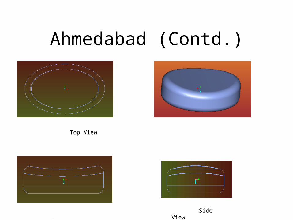
Ahmedabad (Contd.)
Top View
Front View Side View

Kolhapur-ME Design Office
• Called an expert CARPENTER
• Produce a model (check volume etc.)
• Sample the model
and produce a data-
set

Kolhapur(contd.)
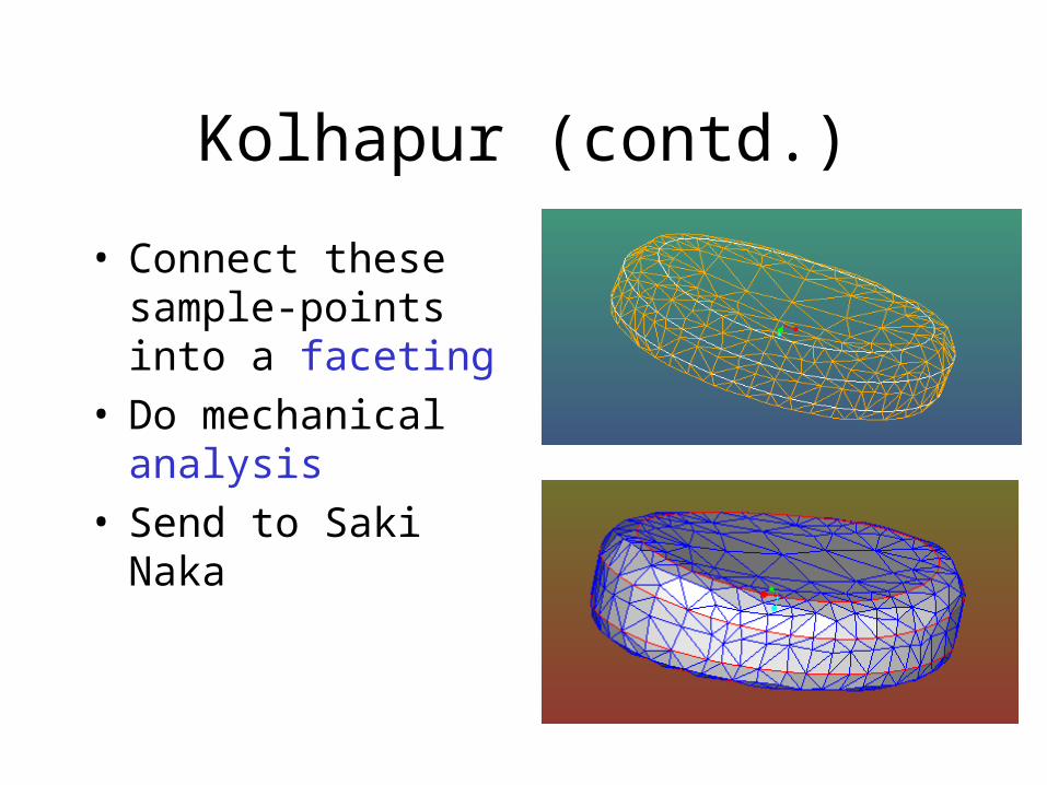
Kolhapur (contd.)
• Connect these sample-points into a faceting
• Do mechanical analysis
• Send to Saki Naka

Saki Naka-Die Manufacturer
• Take the input faceted solid.
• Produce Tool Paths • Produce Die

The Mechanics of it…..

Lucknow-Soaps
• Use the die to manufacture soaps
• Package and transport to points of sale
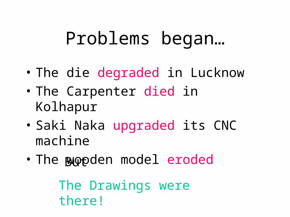
Problems began…
• The die degraded in Lucknow
• The Carpenter died in Kolhapur
• Saki Naka upgraded its CNC machine
• The wooden model eroded
But
The Drawings were there!
So Then….
• The same process was repeated but…
The shape was different!
The customer was suspicious and sales dropped!!!

The Soap Alive !

What was lacking was…A Reproducible Solid-
Model.• Surfaces defn• Tactile/point
sampling• Volume
computation• Analysis

The Solid-Modeller
Modeller
OperationsRepresentations

The mechanical solid-modeller
Operations• Volume
Unions/Intersections• Extrude holes/bosses• Ribs, fillets, blends
etc.
Representation• Surfaces-x,y,z as
functions in 2 parameters
• Edges –x,y,z as functions in 1 parameter

Examples of Solid Models
Torus Lock

Even more examples
Slanted Torus Bearing

Other Modellers-Surface Modelling

Chemical plants.

Chemical Plants (contd.)
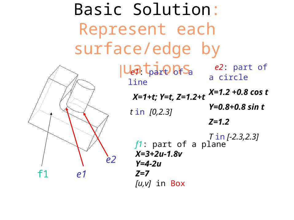
Basic Solution: Represent each surface/edge by equations
e1
e2
e1: part of a line
X=1+t; Y=t, Z=1.2+t
t in [0,2.3]
e2: part of a circle
X=1.2 +0.8 cos t
Y=0.8+0.8 sin t
Z=1.2
T in [-2.3,2.3]
f1
f1: part of a planeX=3+2u-1.8vY=4-2uZ=7[u,v] in Box

A Basic Problem
Construction of defining equations
• Given data points
arrive at a curve approximating
this point-set.• Obtain the
equation of this curve
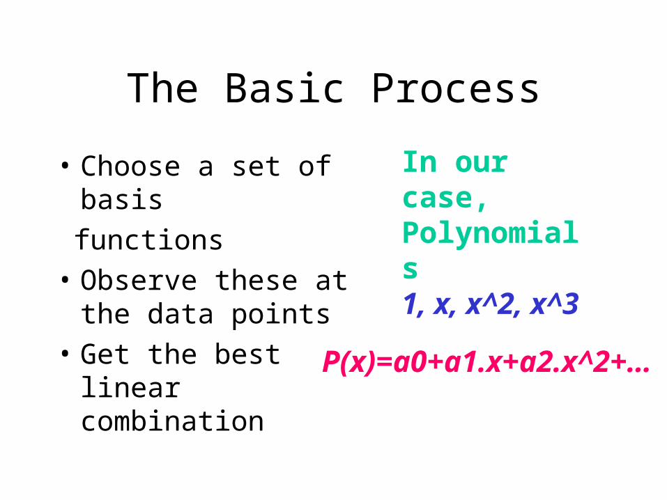
The Basic Process
• Choose a set of basis
functions
• Observe these at the data points
• Get the best linear combination
In our case, Polynomials 1, x, x^2, x^3
P(x)=a0+a1.x+a2.x^2+…

The Observations Process
1 1 1
x 1.2 3.1
x^2 1.44 9.61
=B
v 6.1 2

The Matrix SettingWe have• The basis observations Matrix B which is 5-by-100• The desired observations Matrix v which is 1-by-100We want:• a which is 1-by-5 so that aB is close to v

The minimization
• Minimize least-square error (i.e. distance squared).(6.1-a0.1-a1.1.2-a2.1.44)^2+…+(2-1.a0 - 3.1a1 - 9.61 a2)^2 +…
Thus, this is a quadratic function in the variables
a0,a1,a2,…
And is easily minimized.
1 1 1
x 1.2 3.1
x^2 1.44 9.61
v 6.1 2
a0
a1
a2

A Picture
Essentially, projection of v onto the space spanned by the basis vectors

The calculation
• How does one minimize
1.1 a0^2 +3.7 a0 a1 +6.9 a1^2 ?
• Differentiate!
2.2 a0 + 3.7 a1 =0
3.7 a0 +13.8 a1=0
• Now Solve to get a0,a1

We did this and….
• So we did this for surfaces (very similar) and here are the pictures…

And the surface..
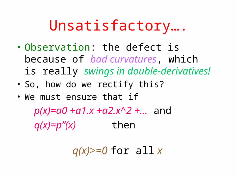
Unsatisfactory….
• Observation: the defect is because of bad curvatures, which is really swings in double-derivatives!
• So, how do we rectify this?• We must ensure that if
p(x)=a0 +a1.x +a2.x^2 +… and
q(x)=p’’(x) then
q(x)>=0 for all x

What does this mean?
q(x)=2.a2+6.a3.x+12.a4.x^2 +…
Thus q(1)>=0, q(2)>=0 means
2.a2 +6.a3 +12.a4 >=0
2.a2 +12.a3+48.a4 >=0
• Whence, we need to pose some linear inequalities on the variables a0,a1,a2,…
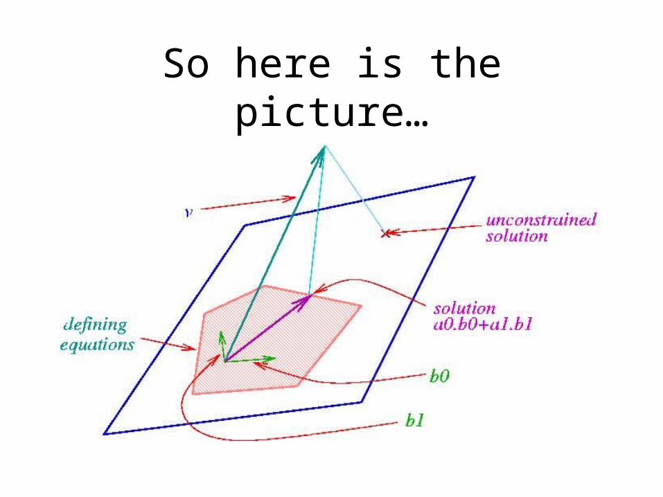
So here is the picture…
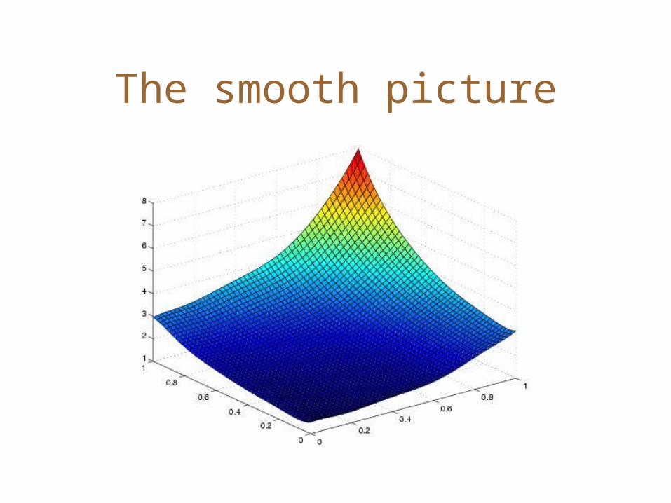
The smooth picture

Another example
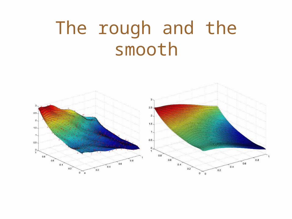
The rough and the smooth

In conclusion
• A brief introduction to CAGD• Curves and Surfaces as equations• Optimization-Least square• Quadratic Programing Linear Constraints Quadratic CostsSee www.cse.iitb.ac.in/sohoni/gsslcourse THANKS


![Maharastra Ground Water Data Analysis - IIT BombayMaharastra Ground Water Data Analysis By Ravi Sagar[10305037] Guided by Prof. Milind Sohoni ... Awale Dug Well 0.760082 7.35 · 2013-2-27](https://static.fdocuments.us/doc/165x107/5adfbd8e7f8b9ad66b8d3e2e/maharastra-ground-water-data-analysis-iit-bombaymaharastra-ground-water-data-analysis.jpg)