Computations of the Expected Euler Characteristic forthe Largest Eigenvalue of a Real non-central Wishart

Matrix

Nobuki Takayama ∗, Lin Jiu †, Satoshi Kuriki ‡, Yi Zhang §

March 27, 2020

Abstract

We give an approximate formula of the distribution of the largest eigenvalue ofreal Wishart matrices by the expected Euler characteristic method for the generaldimension. The formula is expressed in terms of a definite integral with parameters.We derive a differential equation satisfied by the integral for the 2× 2 matrix case andperform a numerical analysis of it.

1 Introduction

For i = 1, . . . , n, let ξi ∈ Rm×1 be independently distributed as the m-dimensional (real)Gaussian distribution Nm(µi,Σ), where µi and Σ are the mean vector and the covariancematrix of ξi, respectively. The (real) Wishart distribution Wm(n,Σ; Ω) is the probabilitymeasure on the cone of m×m positive semi-definite matrices induced by the random matrix

W = ΞΞ>, Ξ = (ξ1, . . . , ξn) ∈ Rm×n.

Here, Ω = Σ−1∑n

i=1 µiµ>i is a parameter matrix. Unless Ω vanishes, the corresponding

distribution is referred to be the non-central (real) Wishart distribution.The largest eigenvalue λ1(W ) of W is used as a test statistic for testing Σ = Im and/or

Ω 6= 0 under the assumption that Σ − Im is positive semi-definite. This test statistic isexpected to have a good power when the matrices Σ− Im and Ω are of low rank.

In the setting of testing hypotheses, the distribution of λ1(W ) is of particular interest; Itcorresponds to the power of the test. When Ω = 0, the celebrated works by A. T. James and

∗Department of Mathematics, Kobe University, Japan. Email: takayama@math.kobe-u.ac.jp†Department of Mathematics and Statistics, Dalhousie University, Canada. Supported by the Austrian

Science Fund (FWF): P29467-N32. Email: lin.jiu@dal.ca‡The Institute of Statistical Mathematics (ISM), Research Organization of Information and Systems

(ROIS), Japan. Supported by JSPS KAKENHI Grant Number 16H02792. Email: kuriki@ism.ac.jp§Corresponding author, Department of Mathematical Sciences, The University of Texas at Dallas (UTD),

USA. Supported by the Austrian Science Fund (FWF): P29467-N32 and the UT Dallas Program: P-1-03246.Email: zhangy@amss.ac.cn

1

other authors show (see e.g., the book by Muirhead [26]) that the cumulative distributionfunction of λ1(W ) can be written as a hypergeometric function of matrix arguments:

Pr(λ1(W ) < x) = cm,ndet

(1

2nxΣ−1

)n/21F1

(1

n;1

2(n+m+ 1);−1

2nxΣ−1

),

where cm,n is a known constant [26, Corollary 9.7.2]. It is well-known that the hypergeometricfunction 1F1 has a series expression in the zonal polynomial Cκ with index κ, which isa partition of an integer. However, in view of numerical calculation, this is less usefulbecause the explicit form of Cκ(X) is not known unless the rank of matrix X is 1 or 2.On account of this difficulty, Hashiguchi et al. [9] recently proposed a holonomic gradientmethod (HGM) for numerical evaluation, which utilizes a holonomic system of differentialequations for computation. However, when Ω 6= 0, the situation is getting worse. Thecumulative distribution function Pr(λ1(W ) < x) can not be expressed as a simple series ofthe zonal polynomials. Hayakawa [10, Corollary 10] provides a formula for the cumulativedistribution function as a series expansion in the Hermite polynomial Hκ with symmetricmatrix argument defined by the Laplace transform of Cκ:

etr(−TT>

)Hκ(T ) =

(−1)|κ|

πmn/2

∫etr(−2iTU>

)etr(−UU>

)Cκ(UU>

)dU, T, U ∈ Rm×n.

The Hermite polynomial Hκ can be written as a linear combination of the zonal polynomialCκ, but the coefficients are not given explicitly [4]. Another approach is the use of invariantpolynomials proposed by Davis [6, 7]. Using the probability density function of the noncentralWishart distribution derived by James [14], the cumulative distribution function of λ1(W )is shown to be proportional to∫

0<W<xIm

|W |(n−m+1)/2−1etr(−1

2(Σ−1W + Ω)

)0F1(n/2; ΩΣ−1W/4) dW.

Dıaz-Garı and Gutierrez-Jaimez [8] show that this has a series expansion in terms of invariantpolynomials. Here, the invariant polynomial is a polynomial in two matrices indexed by twopartitions. Although, in principle, the invariant polynomial can expressed in terms of zonalpolynomials in two matrices, it is hard to utilize this expression for numerical calculation.

In this paper, instead of the direct calculation approach, we will approximate the distri-bution function by means of the expected Euler characteristic heuristic or the Euler char-acteristic method proposed in 2000’s by Adler and Tayler [1] or by Kuriki and Takemura[21]. This is a methodology to approximate the tail upper probability of a random field. Inour problem, since the square root of the largest eigenvalue λ1(W )1/2 is the maximum of aGaussian field

u>Ξv | ‖u‖Rm = ‖v‖Rn = 1,

this method actually works for our purpose ([19], [20]). One can show that the Euler-characteristics method evaluates the quantity

Pr(λ1(W ) ≥ x)− Pr(λ2(W ) ≥ x) + · · ·+ (−1)m−1 Pr(λm(W ) ≥ x),

rather than Pr(λ1(W ) ≥ x). Nevertheless, this formula approximates Pr(λ1(W ) ≥ x) wellwhen x is large because Pr(λi(W ) ≥ x) (i ≥ 2) are negligible when x is large. This is

2

practically sufficient for our purpose since only the upper tail probability is required intesting hypothesis.

In this paper, we deal with the non-central real Wishart matrix. In the multiple-inputmultiple-output (MIMO) problem, the non-central complex Wishart matrix also plays animportant role. The largest eigenvalue of the non-central complex Wishart is much easier tohandle in that case because the explicit formula for the cumulative distribution is given byKang and Alouini [16]. The HGM based on Kang and Alouini’s formula has been proposedin [5].

The organization of the paper is as follows. In Section 2, we give an integral representationformula of the expectation of the Euler characteristic for random matrices of a generalsize. In Section 3, we restrict to the case of 2 × 2 random matrices and study the integralrepresentation derived in Section 2 with the polar coordinate system and investigate it fromnumerical point of view. By virtue of the theory of holonomic systems (e.g., [11]), theintegral representation given in Section 2 satisfies a holonomic system of linear differentialequations. However, its explicit form is not known in general. In Section 4, we come backto the case of 2 × 2 random matrices. We derive a differential equation satisfied by theintegral representation of the expectation of the Euler characteristic with a help of computeralgebra algorithms, systems and perform a numerical analysis of the differential equation.This gives a new efficient method to numerically evaluate the Euler expectation when thenumerical integration is hard to perform. Last but not least, in the appendix, we give a closedformula of the expectation of the Euler characteristic for random matrices of a general sizefor the central and scalar covariance case. The formula is expressed in terms of the Laguerrepolynomial.

2 Expectation of an Euler characteristic number

Let A = (aij) be a real m × n matrix valued random variable (random matrix) with thedensity

p(A)dA, dA =∏

daij.

We assume that p(A) is smooth and n ≥ m ≥ 2. Define a manifold

M = hgT | g ∈ Sm−1, h ∈ Sn−1 ' Sm−1 × Sn−1/ ∼,

where (h, g) ∼ (−h,−g), h and g are column vectors, and hgT is a rank 1 m×n matrix. Set

f(U) = tr(UA) = gTAh, U ∈M,

andMx = hgT ∈M | f(U) = gTAh ≥ x.

Proposition 1. Let A be a random matrix as above. Then the following claims are equiva-lent.

1. The function f(U) has a critical point at U = hgT ;

2. The vectors gT , h are left and right eigenvectors of A, respectively. In other words,there exists a constant c such that gTA = chT , Ah = cg.

3

Moreover, the function f takes the value c at the critical point (g, h).

Proof . We assume that g ∈ Sn−1 and h ∈ Sm−1 are expressed by local coordinates ui andva, respectively, where 1 ≤ i ≤ m− 1 and 1 ≤ a ≤ n− 1. We denote ∂/∂ui by ∂i and ∂/∂vaby ∂a. Since gTg = 1, we have gTi g = 0, where gi = ∂i • g. We will omit •, which means theaction, as long as no confusion arises. Analogously, we have hTa ha = 0, where ha = ∂ah.

Assume that A is a m × n (random real) matrix. Let us consider the function f(U)expressed by the local coordinate (g(u), h(v))

f(g, h) = gTAh, g ∈ Sn−1, h ∈ Sm−1. (1)

At the critical point of f , we have

∂if = giAh = 0, ∂af = gAha = 0.

Since the above equality holds for each i and u is a local coordinate of Sn−1, it implies thatgi’s are linearly independent. Therefore, there exists a constant c such that Ah = cg at thecritical point. Analogously, we can see that there exists a constant d such that ATg = dh.Let us show c = d. We have

(gTA)h = (dhT )h = d(hTh) = d

andgT (Ah) = gT (cg) = c(gTg) = c.

Therefore, we have d = c = f(g, h) at the critical point.Conversely, Ah = cg and ATg = dh at a point (u, v) imply that (g(u), h(v)) is a critical

point of f(g(u), h(v)). //

We take a continuous family of elements of SO(m) parametrized by the first column vec-tor g. In other words, we take a continuous family of orthogonal frames of Rm parametrizedby g ∈ Sm−1. The element of SO(m) is denoted by (g,G) ∈ O(m), where G is an m×(m−1)matrix. Analogously, we take a family (h,H) ∈ SO(n) parametrized by h ∈ Sn−1 , where His an n× (n− 1) matrix parametrized by h. Set

σ = gTAh, B = GT (g)AH(h). (2)

Then the matrix A can be expressed as

A = σghT +G(g)BH(h)T , (3)

which is, intuitively speaking, a partial singular value decomposition. We denote the set ofthe (m− 1)× (n− 1) matrices by M(m− 1, n− 1).

This decomposition above gives coordinate systems for the space of random matrices A’s.Let us introduce them in details. Without loss of generality, we assume that m ≤ n. Wesort the singular values of B by descending order. We denote by λj(B) the j-th singularvalue of the matrix B. For a real number σ, we define

B(i, σ) = B ∈M(m− 1, n− 1) | all the singular values of B are different and non-zero.

λj(B) > σ for all j < i, λj(B) ≤ σ for all j ≥ i.

4

Set

A = A ∈M(m,n) | all the singular values of A are different and non-zero,

andAi = (σ, g, h,B) |σ ∈ R>0, (g, h) ∈ Sm−1 × Sn−1/ ∼, B ∈ B(i, σ).

For a matrix A in A ⊂M(m,n), we sort the singular values of A by descending order

σ(1) > σ(2) > · · · > σ(m) > 0.

Let g(i) and h(i) be the left and right eigenvectors of A for σ(i), respectively. Since g(i) and h(i)

are eigenvectors of AAT and ATA for the eigenvalue σ(i), respectively, it implies that g(i)

and h(i) are uniquely determined modulo the multiplication by ±1. Define a map ϕi from Ato Ai by

ϕi(A) = (σ(i), g(i), h(i), G(g(i))AHT (h(i))). (4)

Note that the matrix G(g(i))AHT (h(i)) lies in B(i, σ(i)) because the singular values of B(i)

agree with those of A excluding σ(i).

Lemma 1. The map ϕi is smooth and isomorphic.

Proof . Define a map ψ from Ai to A by

ψ(σ, g, h,B) = gσhT +G(g)BH(h)T .

By calculation, we see that ϕi ψ and ψ ϕi are identity maps. Then the map ϕi is one-to-one and surjective. Next, we show that the map ψ is smooth. Since we assume that allthe singular values are different, the maps of taking i-th singular value of a given A and aneigenvector for the singular value are smooth on an open connected neighborhood W ⊂ Aof A (by checking the Jacobian does not vanish). Then the inverse map is locally smooth.Hence, ϕi is smooth and isomorphism. //

We are interested in the Euler characteristic number of Mx.

Theorem 1. Suppose that x > 0 and f(U) is a Morse function for almost all A’s. Wefurther assume that if a set is measure zero set with respect to the Lebesgue measure, then itis also a measure zero set with respect to the measure p(A)dA. Then the expectation of theEuler characteristic number E[χ(Mx)] is equal to

1

2

∫ ∞x

σn−mdσ

∫R(m−1)(n−1)

dB

∫Sm−1

GTdg

∫Sn−1

HTdh det(σ2Im−1 −BBT )p(A). (5)

Here, we set GTdg = ∧m−1i=1 GTi dg, HTdh = ∧n−1i=1H

Ti dh, where Gi and Hi are the i-th column

vectors of G and H, respectively, dg = (dg1, . . . , dgm)T and dh = (dh1, . . . , dhn)T .

Note that GTdg and HTdh are O(m) and O(n) invariant measures on Sm−1 and Sn−1,respectively.

5

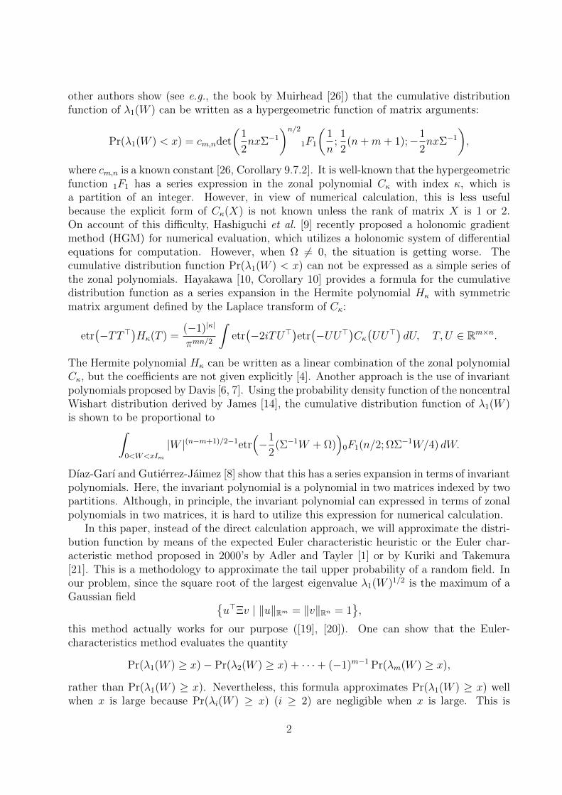
Proof . Without loss of generality, we assume that m ≤ n. According to the Morse theory,if f(U) is a Morse function, which is a smooth function without a degenerated critical point,then we have

χ(Mx) =∑

critical point

1(f(U) ≥ x) sgn det

(−∂i∂jf −∂i∂af−∂a∂if −∂a∂bf

)(6)

=∑

eigenvectors

1(σ ≥ x) sgn det

(σIm −GBHT

−HBTGT σIn

)(7)

=m∑i=1

1(σ(i) ≥ x) sgnσ(i)n−mσ(i)2det(σ(i)2Im−1 −B(i)B(i)T

), (8)

where σ(i) is the i-th singular value of A, g(i) and h(i) are left and right eigenvectors, andB(i) = GT (g(i))AH(h(i)). The equality (6) is the Morse theorem for manifolds with bound-aries. The equalities (6) and (7) can be shown as follows.

Firstly, we have the relation gTi g = 0. By differentiating it with respect to uj, we havegTijg+ gTi gj = 0. Let us evaluate ∂i∂jf . By the expression A = σghT +GBHT , it is equal to

∂i∂jf

= gTijAh

= gTijσghTh+ gTijGBH

Th

= −σgTi gj by HTh = 0.

Next, we evaluate ∂i∂af .

∂i∂af

= gTi Aha

= gTi gσhTha + gTi GBH

Tha

= gTi GBHTha by gTi g = hTha = 0.

Thirdly, we evaluate ∂a∂bf .

∂a∂bf

= gTAhab

= gTgσhThab + gTGBHThab

= −σhTa hb by gTG = 0.

Summarizing these calculation, we have that the Hessian is equal to(−∂i∂jf −∂i∂af−∂i∂af −∂a∂b

)=

(σgTi gj −gTi GBHTha

−hTaHBTGTgi σhTa hb

)=

(g1 · · · gn−1 0

0 h1 · · ·hm−1

)T (σIm −GBHT

−HBTGT σIn

)(g1 · · · gn−1 0

0 h1 · · ·hm−1

).

6

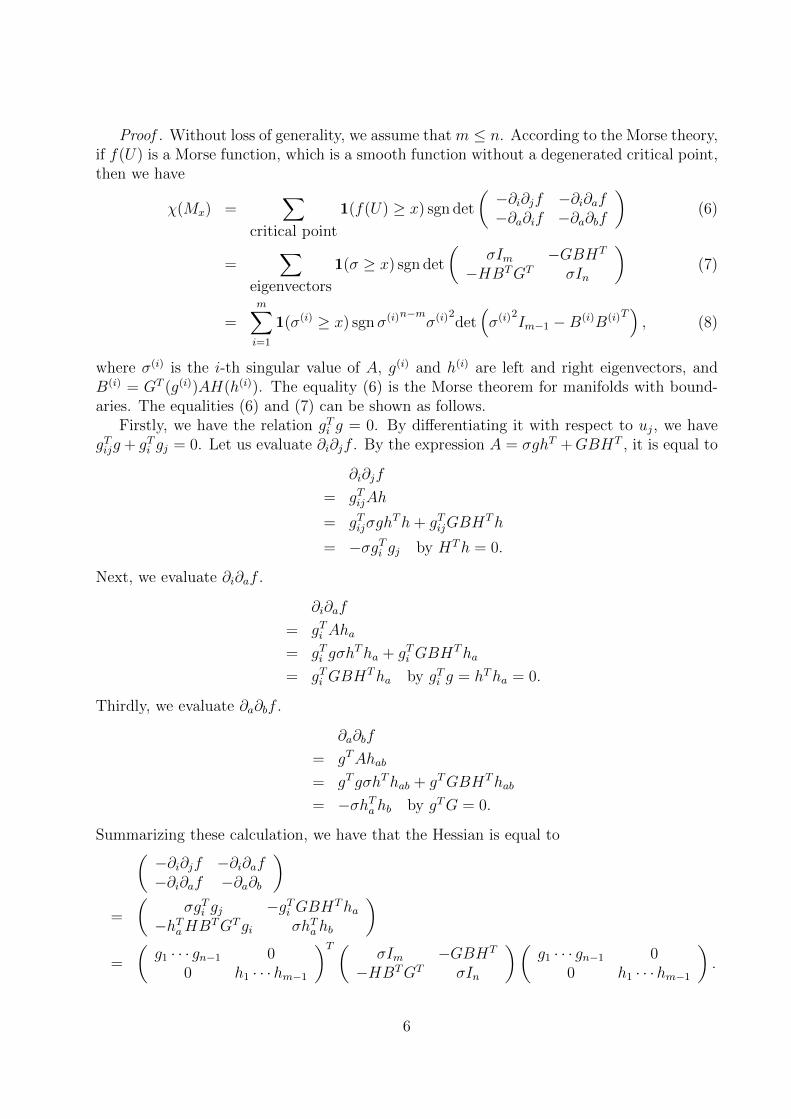
Since det(PP T ) = det(P )2, the sign of the determinant of the Hessian is equal to that of themiddle of the above 3 matrices.

Let us show the equalities (7) and (8). We fix i and omit the superscript (i) in thefollowing discussion. We consider the product of the following two matrices.(

σIm −GBHT

−HBTGT σIn

) (σIm 0

HBTGT σ−1In

).

It is equal to (σ2Im −GBBTGT −σ−1GBHT

−σHBTGT + σHBTGT In

).

Since the left-bottom block is 0, the determinant of this matrix is det(σ2Im−GBBTG). PutC = BBT and G = (g|G). We have

σ2Im −GCGT = σ2Im − G(

0 00 C

)GT .

Since GGT = E, the determinant of the matrix above is equal to σ2 det(σ2Im−1 − C). Insummary, we obtain equalities of (7) and (8).

Let us take the expectation of the Euler characteristic number. Exchanging the sum andthe integral, we have

E[χ(Mx)]

=m∑i=1

∫dAp(A)1(σ(i) ≥ x) sgnσ(i)n−mσ(i)2det

(σ(i)2Im−1 −B(i)B(i)T

).

To evaluate the expectation of the Euler characteristic number, we needs the Jacobianof (3). According to standard arguments in multivariate analysis (see, e.g., [28, (3.19)]), wehave

dA = |det(σ2Im−1 −BBT )| dσGTdgHTdhdB. (9)

Then we have

E[χ(Mx)] (10)

=1

2

m∑i=1

∫ ∞x

σn−mdσ

∫B∈B(i,σ(i))

dB

∫Sm−1

GTdg

∫Sn−1

HTdh det(σ2Im−1 −BBT )p(A).

Note that the factor 1/2 comes from the fact that the multiplicity (g, h) 7→ ghT is 2. PutB(i) = B(i, σ(i)). For i 6= j, since B(i)∩B(j) and R(m−1)(n−1) \

∑mi=1 B(i) are measure zero sets,

we may sum up integral domains for B into one domain as

m∑i=1

∫B∈B(i,σ(i))

det(σ2Im−1 −BBT )p(A)

=

∫B∈M(m−1,n−1)

det(σ2Im−1 −BBT )p(A).

Thus, we derive the conclusion. //

7

Note that the integral (5) does not depend on a choice of G(g) nor H(h). The reason isas follows. The column vectors of the matrix G = G(g) have the length 1 and are orthogonalto the vector g. Let G be a matrix which has the same property. In other words, we assume(g, G) ∈ SO(m). Then there exists an (m − 1) × (m − 1) orthogonal matrix P such thatG = GP and |P | = 1 hold. Taking the exterior product of elements of GTdg = PGTdg, wehave

∧mi=1gTi dg = |P | ∧mi=1 g

Ti dg = ∧mi=1g

Ti dg.

The case for H can be shown analogously.One of the most important examples is that A is distributed as a Gaussian distribution

Nm×n(M,Σ⊗ In). In this case, we have

p(A)dA =1

(2π)mn/2det(Σ)n/2exp−1

2tr(A−M)TΣ−1(A−M)

dA. (11)

Then the largest singular value of A is the square root of the largest eigenvalue of a non-central Wishart matrix Wm(n,Σ,Σ−1MMT ). Substituting (3) and (11) into (5), we have

E[χ(Mx)] =1

2

∫ ∞x

σn−mdσ

∫R(m−1)×(n−1)

dB

∫Sm−1

GTdg

∫Sn−1

HTdhdet(σ2Im−1 −BBT

)× 1

(2π)nm/2det(Σ)n/2exp−1

2tr(σhgT +HBTGT −MT )Σ−1(σghT +GBHT −M)

. (12)

In this expression, number of parameters is m(m+ 1)/2 +mn, so it is over-parametrized.Note that

A = Σ1/2V +M, V = (vij)m×n, vij ∼ N(0, 1) i.i.d.

Let Σ1/2 = P TDP be a spectral decomposition, where D = diag(di). Then we have

PA = DPV + PM.

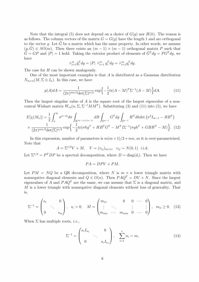
Let PM = NQ be a QR decomposition, where N is m × n lower triangle matrix withnonnegative diagonal elements and Q ∈ O(n). Then PAQT = DV + N . Since the largesteigenvalues of A and PAQT are the same, we can assume that Σ is a diagonal matrix, andM is a lower triangle with nonnegative diagonal elements without loss of generality. Thatis,

Σ−1 =

s1 0. . .

0 sm

, si > 0, M =

m11 0 0 · · · 0...

. . ....

...mmn · · · mmm 0 · · · 0

, mii ≥ 0. (13)

When Σ has multiple roots, i.e.,

Σ−1 =

s1In1 0. . .

0 srInr

,r∑i=1

ni = m, (14)

8

by multiplying diag(P1, . . . , Pr) ∈ O(n1)× · · · ×O(nr) and its transpose from left and right,we can assume

M =

m1In1 0 · · · 0M21 m2In2 0 · · · 0

.... . .

......

Mr−1,1 Mr−1,2 mr−1Inr−1 0 · · · 0Mr1 Mr2 · · · Mr,r−1 mrInr 0 · · · 0

, mi ≥ 0, Mij ∈ Rnj×ni .

(15)Therefore, our problem is formalized as follow: To evaluate (12) with parameters (13) (or(14) and (15)).

In the following sections, we will evaluate the integral representation of the expectationof the Euler characteristic number given in Theorem 1 for some interesting special cases.We can obtain approximate values of the probability of the largest eigenvalue of randommatrices by virtue of them. The Euler characteristic heuristic is

P

(max

g∈Sm−1, h∈Sn−1gTAh ≥ x

)= P

(maxU∈M

f(U) ≥ x)≈ E

[χ(Mx)

].

The condition that f(U) is a Morse function with probability one holds if A has distinct andnon-zero m singular values with probability one.

3 The case of m = n = 2

We derive Theorem 1 in the special case of m = n = 2 by taking explicit coordinates. Thisderivation motivates the proof for the general case discussed in the previous section. Thecase m = n = 2 will be studied numerically in the last section with the holonomic gradientmethod (HGM).

Fix two unit vectors

g = (cos θ, sin θ)T , h = (cosφ, sinφ)T ∈ S1

for 0 ≤ θ, φ < 2π. Define

G =(

cos(θ +

π

2

), sin

(θ +

π

2

))T= (− sin θ, cos θ)T ,

which satisfies

(g,G) =

(cos θ − sin θsin θ cos θ

)∈ SO (2) .

Similarly, we define H =(cos(φ+ π

2

), sin

(φ+ π

2

))T= (− sinφ, cosφ)T . Here, both θ + π

2

and φ+ π2

should be treated as mod 2π, in case the sum is greater than 2π. Now, any 2× 2matrix, say A, can be recovered by

A = σghT + bGHT

with 4 variables (σ, θ, φ, b). We may further assume that σ ∈ R≥0, b ∈ R and φ, θ ∈ [0, 2π).

9

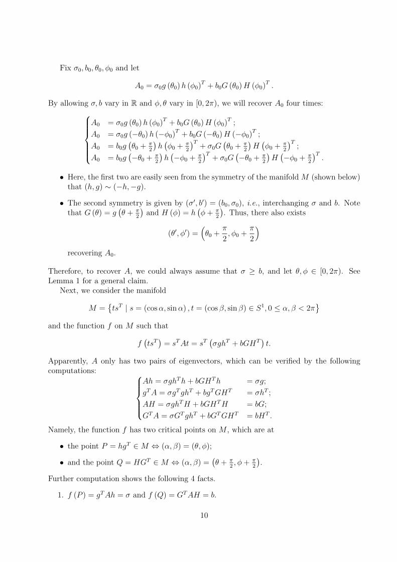
Fix σ0, b0, θ0, φ0 and let

A0 = σ0g (θ0)h (φ0)T + b0G (θ0)H (φ0)

T .

By allowing σ, b vary in R and φ, θ vary in [0, 2π), we will recover A0 four times:A0 = σ0g (θ0)h (φ0)

T + b0G (θ0)H (φ0)T ;

A0 = σ0g (−θ0)h (−φ0)T + b0G (−θ0)H (−φ0)

T ;

A0 = b0g(θ0 + π

2

)h(φ0 + π

2

)T+ σ0G

(θ0 + π

2

)H(φ0 + π

2

)T;

A0 = b0g(−θ0 + π

2

)h(−φ0 + π

2

)T+ σ0G

(−θ0 + π

2

)H(−φ0 + π

2

)T.

• Here, the first two are easily seen from the symmetry of the manifold M (shown below)that (h, g) ∼ (−h,−g).

• The second symmetry is given by (σ′, b′) = (b0, σ0), i.e., interchanging σ and b. Notethat G (θ) = g

(θ + π

2

)and H (φ) = h

(φ+ π

2

). Thus, there also exists

(θ′, φ′) =(θ0 +

π

2, φ0 +

π

2

)recovering A0.

Therefore, to recover A, we could always assume that σ ≥ b, and let θ, φ ∈ [0, 2π). SeeLemma 1 for a general claim.

Next, we consider the manifold

M =tsT | s = (cosα, sinα) , t = (cos β, sin β) ∈ S1, 0 ≤ α, β < 2π

and the function f on M such that

f(tsT)

= sTAt = sT(σghT + bGHT

)t.

Apparently, A only has two pairs of eigenvectors, which can be verified by the followingcomputations:

Ah = σghTh+ bGHTh = σg;

gTA = σgTghT + bgTGHT = σhT ;

AH = σghTH + bGHTH = bG;

GTA = σGTghT + bGTGHT = bHT .

Namely, the function f has two critical points on M , which are at

• the point P = hgT ∈M ⇔ (α, β) = (θ, φ);

• and the point Q = HGT ∈M ⇔ (α, β) =(θ + π

2, φ+ π

2

).

Further computation shows the following 4 facts.

1. f (P ) = gTAh = σ and f (Q) = GTAH = b.

10

2. From

Hessf =

(∂2

∂α2f∂2

∂α∂βf

∂2

∂β∂αf ∂2

∂β2f

)

=

(b−σ) cos(α+β−θ−φ)−(b+σ) cos(α−β−θ+φ)2

(b−σ) cos(α+β−θ−φ)+(b+σ) cos(α−β−θ+φ)2

(b−σ) cos(α+β−θ−φ)+(b+σ) cos(α−β−θ+φ)2

(b−σ) cos(α+β−θ−φ)−(b+σ) cos(α−β−θ+φ)2

,

it follows that det (HessPf) = σ2 − b2 and det (HessQf) = b2 − σ2. Therefore, we see

(a) if x > σ ≥ b, then Mx does not contain any critical points, so χ (Mx) = 0;

(b) if x < b ≤ σ, then Mx contains both critical points, and thus

χ (Mx) = sgn(σ2 − b2

)+ sgn

(b2 − σ2

)= 0;

(c) the only nontrivial case is σ ≥ x ≥ b, then

χ (Mx) = 1 (σ ≥ x ≥ b) sgn(σ2 − b2

).

3. Since

A = σghT + bGHT =

(b sin θ sinφ+ σ cos θ cosφ σ cos θ sinφ− b sin θ cosφσ sin θ cosφ− b cos θ sinφ b cos θ cosφ+ σ sin θ sinφ

),

we have

(dA) = db sin θ sinφ+ σ cos θ cosφ ∧ d (σ cos θ sinφ− b sin θ cosφ)

∧ d (σ sin θ cosφ− b cos θ sinφ) ∧ d (b cos θ cosφ+ σ sin θ sinφ)

=(b2 − σ2

)dσdbdθdφ.

4. Let M =

(m11 0m21 m22

)and Σ =

(1/s1 0

0 1/s2

)such that

A =√

ΣV +M, where V = (vij) , vij ∼ N (0, 1) i. i. d.

Thenp (A) =

s1s2

(2π)2e−

R2 ,

where

R =s1 (b sin θ sinφ+ σ cos θ cosφ−m11)2 + s2 (σ sin θ cosφ− b cos θ sinφ−m21)

2

+ s1 (σ cos θ sinφ− b sin θ cosφ)2 + s2 (b cos θ cosφ+ σ sin θ sinφ−m22)2 .

11

Hence, we have

E (χ (Mx)) =1

2

∫ ∞−∞

dσ

∫ ∞−∞

db

∫ 2π

0

dθ

∫ 2π

0

dφ

(1 (σ ≥ x ≥ b)

︷ ︸︸ ︷sgn

(σ2 − b2

)) ︷ ︸︸ ︷∣∣(b2 − σ2)∣∣

× s1s2

(2π)2e−

R2

=1

2

∫ ∞x

dσ

∫ x

−∞db

∫ 2π

0

dθ

∫ 2π

0

dφ︷ ︸︸ ︷(σ2 − b2

) s1s2(2π)2

e−R2 .

Note that we have∫∞−∞ db · · · =

∫ x−∞ db · · · by an anti-symmetry of σ and b in this case. In

other words, integrals over σ > x > 0, b > x, σ > b and σ > x > 0, b > x, σ < b are canceled.Thus, we have

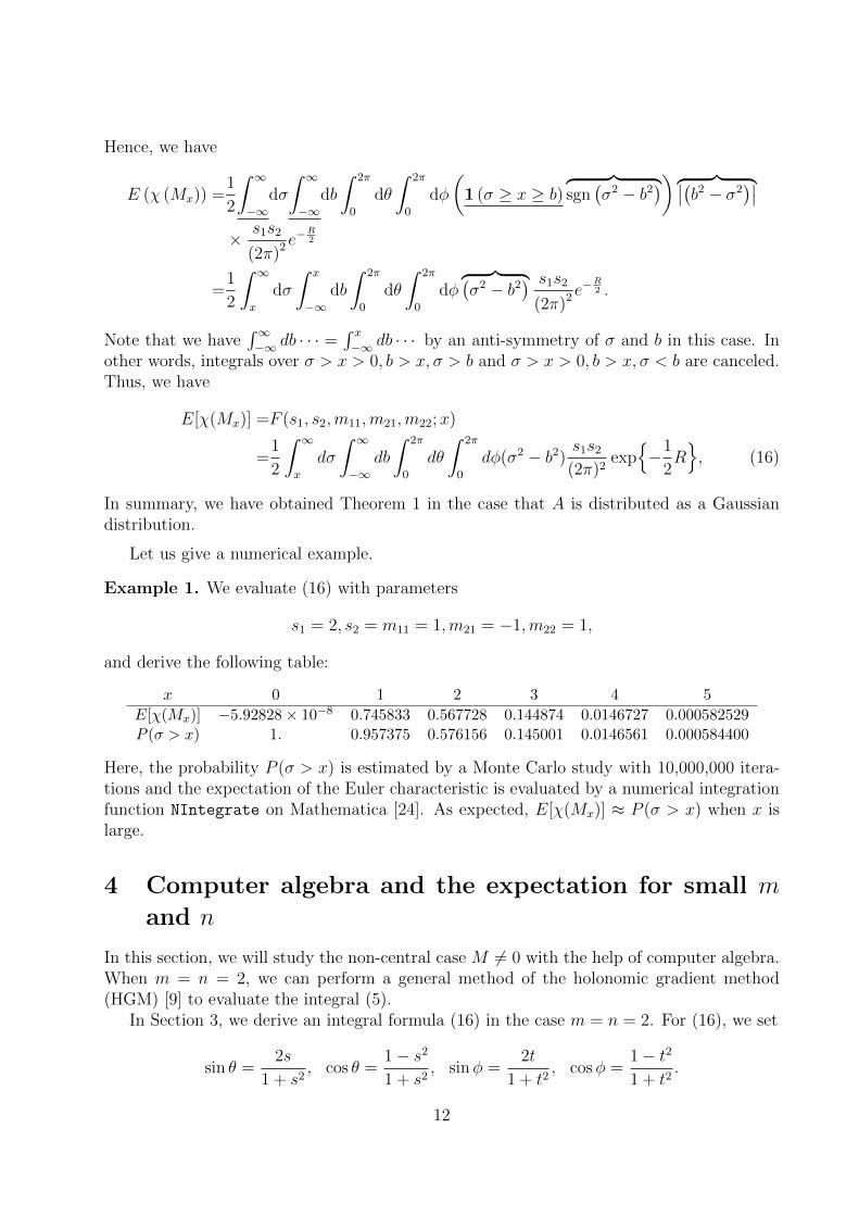
E[χ(Mx)] =F (s1, s2,m11,m21,m22;x)

=1

2

∫ ∞x

dσ

∫ ∞−∞

db

∫ 2π

0

dθ

∫ 2π

0

dφ(σ2 − b2) s1s2(2π)2

exp−1

2R, (16)

In summary, we have obtained Theorem 1 in the case that A is distributed as a Gaussiandistribution.

Let us give a numerical example.

Example 1. We evaluate (16) with parameters

s1 = 2, s2 = m11 = 1,m21 = −1,m22 = 1,

and derive the following table:

x 0 1 2 3 4 5

E[χ(Mx)] −5.92828× 10−8 0.745833 0.567728 0.144874 0.0146727 0.000582529P (σ > x) 1. 0.957375 0.576156 0.145001 0.0146561 0.000584400

Here, the probability P (σ > x) is estimated by a Monte Carlo study with 10,000,000 itera-tions and the expectation of the Euler characteristic is evaluated by a numerical integrationfunction NIntegrate on Mathematica [24]. As expected, E[χ(Mx)] ≈ P (σ > x) when x islarge.

4 Computer algebra and the expectation for small m

and n

In this section, we will study the non-central case M 6= 0 with the help of computer algebra.When m = n = 2, we can perform a general method of the holonomic gradient method(HGM) [9] to evaluate the integral (5).

In Section 3, we derive an integral formula (16) in the case m = n = 2. For (16), we set

sin θ =2s

1 + s2, cos θ =

1− s2

1 + s2, sinφ =

2t

1 + t2, cosφ =

1− t2

1 + t2.

12

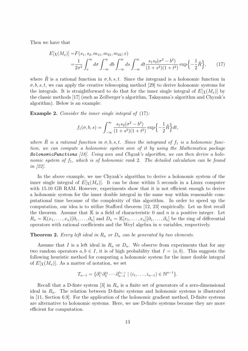
Then we have that

E[χ(Mx)] =F (s1, s2,m11,m21,m22;x)

=1

2π2

∫ ∞x

dσ

∫ ∞−∞

db

∫ ∞−∞

ds

∫ ∞−∞

dts1s2(σ

2 − b2)(1 + s2)(1 + t2)

exp−1

2R, (17)

where R is a rational function in σ, b, s, t. Since the integrand is a holonomic function inσ, b, s, t, we can apply the creative telescoping method [29] to derive holonomic systems forthe integrals. It is straightforward to do that for the inner single integral of E[χ(Mx)] bythe classic methods [17] (such as Zeilberger’s algorithm, Takayama’s algorithm and Chyzak’salgorithm). Below is an example:

Example 2. Consider the inner single integral of (17):

f1(σ, b, s) =

∫ ∞−∞

s1s2(σ2 − b2)

(1 + s2)(1 + t2)exp−1

2Rdt,

where R is a rational function in σ, b, s, t. Since the integrand of f1 is a holonomic func-tion, we can compute a holonomic system ann of it by using the Mathematica packageHolonomicFunctions [18]. Using ann and Chyzak’s algorithm, we can then derive a holo-nomic system of f1, which is of holonomic rank 2. The detailed calculation can be foundin [22].

In the above example, we use Chyzak’s algorithm to derive a holonomic system of theinner single integral of E[χ(Mx)]. It can be done within 5 seconds in a Linux computerwith 15.10 GB RAM. However, experiments show that it is not efficient enough to derivea holonomic system for the inner double integral in the same way within reasonable com-putational time because of the complexity of this algorithm. In order to speed up thecomputation, our idea is to utilize Stafford theorem [12, 23] empirically. Let us first recallthe theorem. Assume that K is a field of characteristic 0 and n is a positive integer. LetRn = K(x1, . . . , xn)[∂1, . . . , ∂n] and Dn = K[x1, . . . , xn][∂1, . . . , ∂n] be the ring of differentialoperators with rational coefficients and the Weyl algebra in n variables, respectively.

Theorem 2. Every left ideal in Rn or Dn can be generated by two elements.

Assume that I is a left ideal in Rn or Dn. We observe from experiments that for anytwo random operators a, b ∈ I, it is of high probability that I = 〈a, b〉. This suggests thefollowing heuristic method for computing a holonomic system for the inner double integralof E[χ(Mx)]. As a matter of notation, we set

Tn−1 = ∂i11 ∂i22 · · · ∂in−1

n−1 | (i1, . . . , in−1) ∈ Nn−1.

Recall that a D-finte system [3] in Rn is a finite set of generators of a zero-dimensionalideal in Rn. The relation between D-finite systems and holonomic systems is illustratedin [11, Section 6.9]. For the application of the holonomic gradient method, D-finite systemsare alternative to holonomic systems. Here, we use D-finite systems because they are moreefficient for computation.

13

Heuristic 1. Given a D-finite system G in Rn, compute another D-finite system G1 in Rn−1such that G1 ⊂ (Rn ·G+ ∂nRn) ∩Rn−1.

1. Choose two finite support set S1, S2 ∈ Tn−1.

2. Using the polynomial ansatz method [17, Section 3.4], check whether there exist tele-scopers P1, P2 ∈ Rn−1 of G with support sets S1, S2 or not. If P1 and P2 exist, then goto next step. Otherwise, go to step 1.

3. Compute the Grobner basis G1 of P1, P2 with respect to a term order in Tn−1. If G1

is D-finite, then output G1. Otherwise, go to step 1.

In the above heuristic method, we need to find two finite support set S1, S2 ∈ Tn−1through trial and error so that it will terminate and finish in a reasonable computationaltime. Next, we show how to use it to derive a D-finite system for the inner double integralof E[χ(Mx)].

Example 3. Consider the inner double integral of (17):

f2(σ, b) =

∫ ∞−∞

f1(σ, b, s)ds (18)

where f1(σ, b, s) is defined in Example 2.Let G be a D-finite system of f1, which is derived from Example 2. Using G and the

polynomial ansatz method, we find two nonzero annihilators P1 and P2 for f2 with supportsets S1 and S2, respectively, where

S1 = 1, ∂b, ∂σ, ∂2b , ∂b∂σ, ∂2σ, ∂3σ,S2 = S1 ∪ ∂2b∂σ, ∂b∂2σ, ∂3b.

Then we compute the Grobner basis G1 of P1, P2 in Q(b, σ)[∂b, ∂σ] with respect to atotal degree lexicographic order. We find that G1 is a D-finite system of holonomic rank 6.The details of the calculation can be found in [22].

In the above example, we specify the parameters in the integrand as that in Exam-ple 1. Using Heuristic 1, we can further compute a holonomic system for the inner doubleintegral of E[χ(Mx)] without specifying those parameters (pars). It is much more efficientthan Chyzak’s algorithm. Below is a table for the comparison between Chyzak’s algorithm(chyzak) and Heuristic 1 (heuristic) for the computational time (seconds).

# pars 0 1 2 3 4 5chyzak 976 9.8323× 104 - - - -

heuristic 43.49 394.4 8527 4.3957× 105 - 1.5519× 106

Next, we use Heuristic 1 to derive a D-finite system of the inner triple integral of E[χ(Mx)]and then numerically solve the corresponding ordinary differential equation. Finally, we usenumerical integration to evaluate E[χ(Mx)].

14

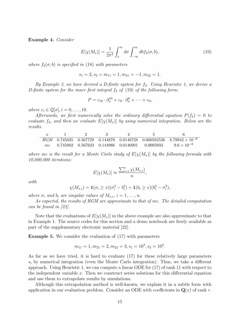
Example 4. Consider

E[χ(Mx)] =1

2π2

∫ ∞x

dσ

∫ ∞−∞

dbf2(σ, b), (19)

where f2(σ, b) is specified in (18) with parameters

s1 = 2, s2 = m11 = 1,m21 = −1,m22 = 1.

By Example 3, we have derived a D-finite system for f2. Using Heuristic 1, we derive aD-finite system for the inner first integral f3 of (19) of the following form:

P = c10 · ∂10σ + c9 · ∂9σ + · · ·+ c0,

where ci ∈ Q[σ], i = 0, . . . , 10.Afterwards, we first numerically solve the ordinary differential equation P (f3) = 0 to

evaluate f3, and then we evaluate E[χ(Mx)] by using numerical integration. Below are theresults.

x 1 2 3 4 5 6

HGM 0.745835 0.567729 0.144879 0.0146728 0.000582526 8.79942× 10−6

mc 0.745802 0.567623 0.144986 0.0146901 0.0005933 9.6× 10−6

where mc is the result for a Monte Carlo study of E[χ(Mx)] by the following formula with10,000,000 iterations:

E[χ(Mx)] ≈∑n

i=1 χ(Mx,i)

n,

withχ(Mx,i) = 1(σi ≥ x)(σ2

i − b2i ) + 1(bi ≥ x)(b2i − σ2i ),

where σi and bi are singular values of Mx,i, i = 1, . . . , n.As expected, the results of HGM are approximate to that of mc. The detailed computation

can be found in [22].

Note that the evaluations of E[χ(Mx)] in the above example are also approximate to thatin Example 1. The source codes for this section and a demo notebook are freely available aspart of the supplementary electronic material [22].

Example 5. We consider the evaluation of (17) with parameters

m11 = 1,m21 = 2,m22 = 3, s1 = 103, s2 = 102.

As far as we have tried, it is hard to evaluate (17) for these relatively large parameterssi by numerical integration (even the Monte Carlo integration). Thus, we take a differentapproach. Using Heuristic 1, we can compute a linear ODE for (17) of rank 11 with respect tothe independent variable x. Then we construct series solutions for this differential equationand use them to extrapolate results by simulations.

Although this extrapolation method is well-known, we explain it in a subtle form withapplication in our evaluation problem. Consider an ODE with coefficients in Q(x) of rank r.

15

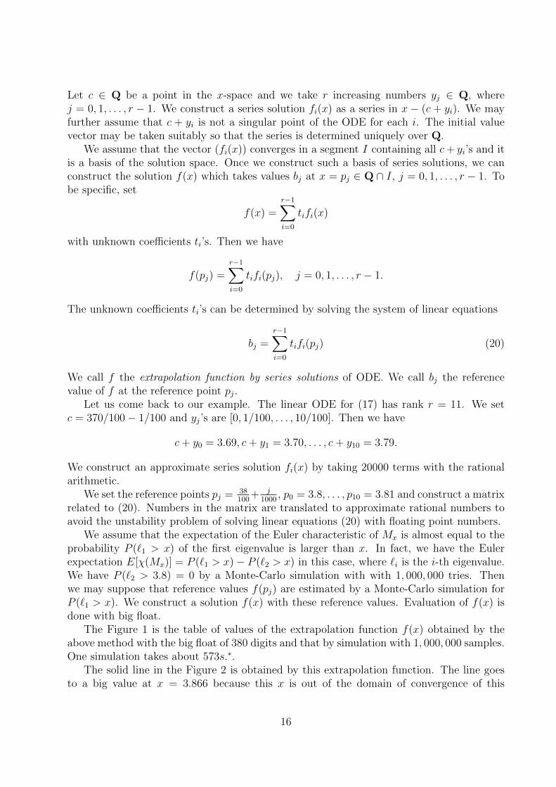
Let c ∈ Q be a point in the x-space and we take r increasing numbers yj ∈ Q, wherej = 0, 1, . . . , r − 1. We construct a series solution fi(x) as a series in x − (c + yi). We mayfurther assume that c + yi is not a singular point of the ODE for each i. The initial valuevector may be taken suitably so that the series is determined uniquely over Q.

We assume that the vector (fi(x)) converges in a segment I containing all c+ yi’s and itis a basis of the solution space. Once we construct such a basis of series solutions, we canconstruct the solution f(x) which takes values bj at x = pj ∈ Q ∩ I, j = 0, 1, . . . , r − 1. Tobe specific, set

f(x) =r−1∑i=0

tifi(x)

with unknown coefficients ti’s. Then we have

f(pj) =r−1∑i=0

tifi(pj), j = 0, 1, . . . , r − 1.

The unknown coefficients ti’s can be determined by solving the system of linear equations

bj =r−1∑i=0

tifi(pj) (20)

We call f the extrapolation function by series solutions of ODE. We call bj the referencevalue of f at the reference point pj.

Let us come back to our example. The linear ODE for (17) has rank r = 11. We setc = 370/100− 1/100 and yj’s are [0, 1/100, . . . , 10/100]. Then we have

c+ y0 = 3.69, c+ y1 = 3.70, . . . , c+ y10 = 3.79.

We construct an approximate series solution fi(x) by taking 20000 terms with the rationalarithmetic.

We set the reference points pj = 38100

+ j1000

, p0 = 3.8, . . . , p10 = 3.81 and construct a matrixrelated to (20). Numbers in the matrix are translated to approximate rational numbers toavoid the unstability problem of solving linear equations (20) with floating point numbers.

We assume that the expectation of the Euler characteristic of Mx is almost equal to theprobability P (`1 > x) of the first eigenvalue is larger than x. In fact, we have the Eulerexpectation E[χ(Mx)] = P (`1 > x)− P (`2 > x) in this case, where `i is the i-th eigenvalue.We have P (`2 > 3.8) = 0 by a Monte-Carlo simulation with with 1, 000, 000 tries. Thenwe may suppose that reference values f(pj) are estimated by a Monte-Carlo simulation forP (`1 > x). We construct a solution f(x) with these reference values. Evaluation of f(x) isdone with big float.

The Figure 1 is the table of values of the extrapolation function f(x) obtained by theabove method with the big float of 380 digits and that by simulation with 1, 000, 000 samples.One simulation takes about 573s.∗.

The solid line in the Figure 2 is obtained by this extrapolation function. The line goesto a big value at x = 3.866 because this x is out of the domain of convergence of this

16

x f(x) simulation3.8133 0.051146 0.0511763.8166 0.047517 0.0476953.82 0.044120 0.044515

Figure 1: Numerical evaluation by extrapolation series

3.6 3.7 3.8 3.9 4.0

0.0

0.1

0.2

0.3

0.4

0.5

0.6

0.7

3.6 3.7 3.8 3.9 4.0

0.0

0.1

0.2

0.3

0.4

0.5

0.6

0.7

3.6 3.7 3.8 3.9 4.0

0.0

0.1

0.2

0.3

0.4

0.5

0.6

0.7

x

E[c

hi(M

x)]

Figure 2: The extrapolation function with 20000 terms. Solid line is the extrapolationfunction, which diverges when x > 3.8633. Dots are values by simulations.

approximate series. Dots are values obtained by simulation and that on the thick solid lineare values used as reference values to obtain the extrapolation function.

The time to obtain the series fi with 20, 000 terms is 5661s†. The time to evaluate theextrapolation function at 61 points is 14.03s. On the other hand, if we want to obtainsimulation values at 61 points, we need about 573 × 61 = 34953s. Thus, our extrapolationmethod has advantages when we want to evaluate the function E[χ(Mx)] for many x.

∗R and the package mnormt on a machine with Intel Xeon CPU(2.70GHz) and 256G memory.†Risa/Asir on a machine with Intel Xeon CPU(2.70GHz) and 256G memory.

17

Appendix: The central case with a scalar covariance:

Selberg type integral and Laguerre polynomials

In this appendix, we assume that M = 0 (central) and Σ in (13) is a scalar matrix , and studythis case by special functions. Under these assumptions, we will show that the expectationof the Euler characteristic can be expressed in terms of a Selberg type integral, which isequal to a Laguerre polynomial in view of the works by K.Aomoto [2] and J.Kaneko [15]

Theorem 3. SetMx = hgT | gTAh ≥ x, h, g ∈ Sm−1.

Assume that the distribution of m×m random matrices A is the Gaussian distribution withaverage 0 and the covariance Im/s. In other words, we have

p(A) ∼ exp

(−1

2tr (sATA)

).

Then we have

E[χ(Mx(s))] =5∏i=1

ci

∫ +∞

x

exp(−s

2σ2)

1F1(−(m− 1), 1; sσ2)dσ, (21)

where c1, c2, c3, c4, c5 are given by (22), (23), (26), (29), (34), respectively.

Proof . For g, h ∈ Sm−1, set

G =(g G

)∈ O(m), g is a column vector,

H =(h H

)∈ O(n), h is a column vector.

Then the m×m matrix A can be written as

A = G

(σ 00 B

)HT .

We denote by B the middle matrix in the above expression.Set etr(X) = exp(tr(X)) and S = Σ−1. We consider the central case M = 0 in (12).

Since tr(PQ) = tr(QP ) and HT H = E, we have

etr(−1

2ATSA)

= etr(−1

2HBT GTSGBHT )

= etr(−1

2SGBHT HBT GT )

= etr(−1

2SG(BBT )GT ).

18

It follows from Theorem 1 with p(A) being the normal distribution that

E[χ(Mx)] = c1(S)

∫ ∞x

σn−mdσ

∫R(m−1)(n−1)

dB

∫Sm−1

GTdg

∫Sn−1

HTdh

det(σ2Im−1 −BBT )etr(−1

2SG(BBT )GT ),

where

c1(S) =1

2· 1

(2π)nm/2det(S−1)n/2. (22)

We denote by Gi the i-th column vector of G and by dg the column vector of the differentialforms dgi. Define

GTdg = ∧m−1i=1 GTi · dg.

It is an invariant measure for the rotations on Sm−1 [13, Theorem 4.2]. We may define HTdhanalogously.

Moreover, since S = sIm, we have

etr(−1

2SG(BBT )GT ) = etr(−s

2BBT ).

Since there is no G,H involved in the right side of the above identity, we can separate thefollowing integral

c2(m) =

∫Sm−1

GTdg

∫Sm−1

HTdh =

(2πm/2

Γ(m/2)

)2

. (23)

Therefore, we only need to evaluate the integral∫R(m−1)2

dB det(σ2Im−1 −BBT )etr(−s

2BBT

). (24)

We denote the integral above by q(s;σ). In terms of q(s;σ), we have

E[χ(Mx)] = c1(S)c2(m)

∫ ∞x

q(s;σ)dσ.

We make the singular value decomposition of the matrix B as B = PLQT , where thematrices P,Q ∈ O(m− 1), L = diag(`1, . . . , `m−1) (see, e.g., [13] and [28, (3.1)]). It followsfrom [28, (3.1)] that

dB =∏

1≤i<j≤m−1

(`2i − `2j)

(m−1∏i=1

d`i

)∧ ω,

ω = ∧1≤i≤m−1,i<j≤m−1P Tj dPi ∧1≤i≤m−1,i<j≤m−1 QT

j dQi,

when `1 ≥ `2 ≥ · · · ≥ `m−1. Here, Pi and Qi are i-th column vectors, respectively. Since

det(σ2Im−1 − PLQTQLTP T ) = det(P (σ2Im−1 − LLT )P T ) = det(σ2Im−1 − LLT ),

19

and

etr(−s

2BBT

)= exp

(−s

2σ2)

etr(−s

2BBT

)= exp

(−s

2σ2)

etr(−s

2PLQTQLTP T

)= exp

(−s

2σ2)

exp(−s

2LLT

),

we have

q(s;σ) = c3(m,σ)

∫L∈Rm−1

∏1≤i<j≤m−1

|`2i − `2j |m−1∏i=1

(σ2 − `2i ) exp(−s

2

∑`2i

)m−1∏i=1

d`i, (25)

where

c3(m;σ) =1

(m− 1)!2m−12m−1exp

(−s

2σ2)∫

O(m−1)

∫O(m−1)

ω (26)

=1

(m− 1)!2m−1exp

(−s

2σ2)(

2m−2m−1∏k=2

πk/2

Γ(k/2)

)2

.

In (26), there is a constant (m − 1)!2m−12m−1 involved in the denominator because in thiscase (m − 1)!2m−1 copies of the domain `1 ≥ `2 ≥ . . . ≥ `m−1 ≥ 0 cover Rm−1, and thecorrespondence between the coordinates of B and that of its singular value decompositionis 1/2m−1. Moreover, note that the volume of O(m− 1) is two times of that of SO(m− 1).

In (25), we make a change of variables by `′i = `2i . Then we have d`′i = 2`id`i, and

d`i =1

2√`′id`′i.

Furthermore, we have

q(s;σ) = c3(m;σ)

∫L′∈Rm−1

≥0

∏`′i−1/2 ∏

1≤i<j≤m−1

|`′i − `′j|m−1∏i=1

(σ2 − `′i)

× exp(−s

2

∑`′i

)m−1∏i=1

d`′i. (27)

Put `′i = 2s`′′i and factor out s > 0. Then it follows from d`′i = 2

sd`′′i that

q(s;σ) = c3(m;σ)c4(m, s)q(s;σ),

where

q(s;σ) =

∫L′′∈Rm−1

≥0

∏`′′i−1/2 ∏

1≤i<j≤m−1

|`′′i − `′′j |m−1∏i=1

(σ2s

2− `′′i ) exp

(−∑

`′′i

)m−1∏i=1

d`′′i , (28)

20

and

c4(m, s) = (s/2)(m−1)/2(s/2)−12(m−1)(m−2)(s/2)−(m−1)(s/2)−(m−1) = (s/2)−

12(m2−1). (29)

This integral (28) can be expressed as a polynomial in σ. Let us derive differential equationsfor this integral and express it in terms of a special polynomial. We utilize the result byAomoto [2] and its generalization [15] by Kaneko. In [15], a system of differential equations,special values, and an expansion in terms of Jack polynomials are given for the integral∫

[0,1]m−1

∏1≤i≤m−1,1≤k≤r

(`i − σk)µD(`1, . . . , `m−1)d`1 · · · d`m−1, (30)

D =m−1∏i=1

`λ1i (1− `i)λ2∏

1≤i<j≤m−1

|`i − `j|λ,

when µ = 1 or µ = −λ/2. Let us make the coordinate change `i = yi/N , λ2 = N , σi = τi/N .Then we have d`i = dyi/N , (1− `i)λ = (1− yi/N)N ,

(1− yi/N)N → exp(−yi), N →∞.

The integral (30) becomes

cN

∫[0,N ]m−1

∏1≤i≤m−1,1≤k≤r

(yi − τk)µD(y1, . . . , ym−1)dy1 · · · dym−1,

D =m−1∏i=1

yλ1i (1− yi/N)N∏

1≤i<j≤m−1

|yi − yj|λ, cN = N−r(m−1)−(m−1)−λ1(m−1)−λ(m−1)(m−2)/2.

When N →∞, this above integral divided by cN converges to∫Rm−1≥0

∏1≤i≤m−1,1≤k≤r

(yi − τk)µD(y1, . . . , ym−1)dy1 · · · dym−1, (31)

D =m−1∏i=1

yλ1i exp(−m−1∑i=1

yi)∏

1≤i<j≤m−1

|yi − yj|λ.

Let us apply this limiting procedure to derive a differential equation for the above integral.When r = µ = 1, the differential equation for the integral (30) is

σ(1− σ)∂2σ + (c− (a+ b+ 1)σ)∂σ − ab, (32)

where a = −(m − 1), b = 2λ(λ1 + λ2 + 2) + (m − 1) + 1, c = 2

λ(λ1 + 1). This is the Gauss

hypergeometric equation. Set λ2 = N , σ = zN

. Then we can find the limit of this equationwhen N → ∞. In fact, it can be performed as follows. Set θz = z∂z. Note that (32) isinvariant by the scalar multiplication of z. Then the limit of

θz(θz +2

λ(λ1 + 1)− 1)− z

N(θz − (m− 1))(θz +

2

λ(N + λ1 + 2) + (m− 1) + 1)

21

when N →∞ is

θz(θz +2

λ(λ1 + 1)− 1)− 2

λz(θz − (m− 1)).

In particular, when λ = 1 and λ1 = −1/2, it is

θ2z − 2z(θz − (m− 1)).

A polynomial solution of the above equation can be written as

c5(m) · 1F1(−(m− 1), 1; 2z)

with a constant c5(m). Therefore, it follows from (28), (31) and the above argument that

q(s;σ) = c3(m;σ)c4(m, s)c5(m) · 1F1(−(m− 1), 1;σ2s) (33)

= c3(m;σ)c4(m, s)c5(m)(1 +−(m− 1)

1(σ2s) +

(m− 1)(m− 2)

(2!)2(σ2s)2

+−(m− 1)(m− 2)(m− 3)

(3!)2(σ2s)3 + · · ·+ (−1)m−1(m− 1)!

((m− 1)!)2(σ2s)m−1

),

where

c5(m) = (the expression (28))|σ=0=

m−1∏i=1

Γ(1 + i

2

)Γ(32

+ i−12

)Γ(32

) (34)

by taking a limit of the Selberg integral formula [27]. //

Let us make a numerical evaluation by utilizing Theorem 3 when m = 3. When m = 3,we have

c1c2c3c4c5 = 2√

2/π√s exp(−σ2s/2).

Since

u(s, k, x) =

∫ +∞

x

exp(−σ2s/2)σ2kdσ

= Γ(k + 1/2)

(2

s

)k+1/21

2

∫ +∞

x2

yk+1/2−1 exp(−y/(2/s))dyΓ(k + 2)(2/s)k+1/2

,

where the integral of the second line is equal to the upper tail probability of the Gammadistribution with the scale 2/s and the shape k + 1/2. It follows from Theorem 3 that theexpectation E[χ(Mx)] is equal to

2√

2/π√s

(u(s, 0, x)− 2su(s, 1, x) +

s2

2u(s, 2, x)

). (35)

An R code for evaluating E[χ(Mx)] in this case is as follows.

ug2<-function(s,k,x)

return(pgamma(x^2, scale=2/s, shape=k+1/2, lower = FALSE)*

gamma(k+1/2)*(2/s)^(k+1/2)/2);

22

ec3<-function(x,s)

cc<- 2*(2/pi)^(1/2)*s^(1/2);

c5<-1;

return(cc*c5*

(ug2(s,0,x)-2*s*ug2(s,1,x)+(1/2)*s^2*ug2(s,2,x)));

## Draw a graph

curve(ec3(x,1),from=1,to=10)

When s = 1, some values are as follows:

x E[χ(Mx)] simulation (with 100000 tries)3 0.215428520 0.2170724 0.016122970 0.0161955 0.000357368 0.000386

Acknowledgement

We deeply thank Christoph Koutschan, who is the author of the package HolonomicFunctionsused in this paper, for his helps and encouragements. We also acknowledge the AustrianScience Fund (FWF): P29467-N32 since the second author and the corresponding author aresupported by it.

References

[1] R. J. Adler, J. E. Taylor, Random fields and geometry, Springer, 2007.

[2] K. Aomoto, Jacobi Polynomials associated with Selberg Integrals, SIAM Journal onMathematical Analysis 18 (1987), 545–549.

[3] S. Chen, M. Kauers, Z. Li, and Y. Zhang, Apparent singularities of D-finite systems,Journal of Symbolic Computation, in press, (2019).

[4] Y. Chikuse, Properties of Hermite and Laguerre polynomials in matrix argument andtheir applications, Linear Algebra and its Applications 176 (1992), 237–260.

[5] F. H. Danufane, C. Siriteanu, K. Ohara, N. Takayama, Holonomic gradient method-based CDF evaluation for the largest eigenvalue of a complex noncentral Wishart matrix,arxiv:1707.02564.

[6] A. W. Davis, Invariant polynomials with two matrix arguments extending the zonalpolynomials: Applications to multivariate distribution theory, Annals of the Instituteof Statistical Mathematics, A31 (1979) 465–485.

[7] A. W. Davis, Invariant polynomials with two matrix arguments: extending the zonalpolynomials, in: P. R. Krishnaiah (Ed.), Multivariate Analysis V, North-Holland Pub-lishing Company, 1980, pp. 287–299.

23

[8] J. A. Dıaz-Garcıa and R. Gutierrez-Jaimez, On Wishart distribution: Some extensions,Linear Algebra and its Applications, 435 (6) (2011), 1296–1310.

[9] H. Hashiguchi, Y. Numata, N. Takayama, A. Takemura, Holonomic gradient method forthe distribution function of the largest root of a Wishart matrix, Journal of MultivariateAnalysis, 117 (2013), 296–312.

[10] T. Hayakawa, On the distribution of the latent roots of a positive definite randomsymmetric matrix I, Annals of the Institute of Statistical Mathematics 21 (1969), 1–21.

[11] T. Hibi et al., Grobner Bases: Statistics and Software Systems, Springer, (2013).

[12] A. Hillebrand, W. Schmale, Towards a effective version of a theorem of Stafford, Journalof Symbolic Computation 32 (2001), 699–716.

[13] A. T. James, Normal Multivariate Analysis and the Orthogonal Group, The Annals ofMathematical Statistics (1954), 40–75.

[14] A. T. James, The Non-Central Wishart Distribution, Proceedings of the Royal Societyof London, Series A, Mathematical and Physical Sciences, 229 (1955), 364–366.

[15] J. Kaneko, Selberg Integrals and Hypergeometric Functions associated with Jack Poly-nomials, SIAM Journal on Mathematical Analysis 24 (1993), 1086–1110.

[16] M. Kang, M. S. Alouini, Largest eigenvalue of complex Wishart matrices and perfor-mance analysis of MIMO MRC systems, IEEE Journal on Selected Areas in Communi-cations 21 (2003), 418–426.

[17] C. Koutschan, Advanced applications of the holonomic systems approach, PhD thesis,Johannes Kepler University Linz, (2009).

[18] C. Koutschan, HolonomicFunctions user’s guide, Technical Report 10-01, RISC ReportSeries, Johannes Kepler University Linz, Austria, (2010).http://www.risc.jku.at/publications/download/risc 3934/hf.pdf

[19] S. Kuriki, A. Takemura, Tail probabilities of the maxima of multilinear forms and theirapplications, The Annals of Statistics 29 (2001), 328–371.

[20] S. Kuriki, A. Takemura, Euler characteristic heuristic for approximating the distribu-tion of the largest eigenvalue of an orthogonally invariant random matrix, Journal ofStatistical Planning and Inference 138 (2008), 3357–3378.

[21] S. Kuriki, A. Takemura, Volume of tubes and the distribution of the maximum of aGaussian random field, Selected Papers on Probability and Statistics, American Math-ematical Society Translations Series 2, 227 (2009), 25–48.

[22] N. Takayama, L. Jiu, S. Kuriki, N. Takayama, Y. Zhang, Supplementary electronicmaterial to the article Euler Characteristic Method for the Largest Eigenvalue of aRandom Matrix. https://yzhang1616.github.io/ec1/ec1.html

24

[23] A. Leykin, Algorithmic proofs of two theorems of Stafford. Journal of Symbolic Com-putation 38 (2004), 1535–1550.

[24] Mathematica, Version 11.0, Wolfram Research, Inc., Champaign, IL, 2016.

[25] M. Morse, S. S. Cairns, Critical point theory in global analysis and differential topology:an introduction, Academic Press, 1969

[26] R. J. Muirhead, Aspects of multivariate statistical theory, Wiley, 2005.

[27] A. Selberg, Remarks on a multiple integral, Norsk Matematisk Tidsskrift 26 (1944),71–78.

[28] A. Takemura, S. Kuriki, Shrinkage to smooth non-convex cone: principal componentanalysis as Stein estimation, Communications in Statistics: Theory and Methods 28(1999), 651–669.

[29] D. Zeilberger, The method of creative telescoping, Journal of Symbolic Computation11 (1991), 195–204.

25