LUND UNIVERSITY

PO Box 117221 00 Lund+46 46-222 00 00

Computationally Efficient Robust Adaptive Beamforming for Passive Sonar

Somasundaram, Samuel; Pilkington, Adrian; Hart, Leslie; Butt, Naveed; Jakobsson, Andreas

2015

Link to publication

Citation for published version (APA):Somasundaram, S., Pilkington, A., Hart, L., Butt, N., & Jakobsson, A. (2015). Computationally Efficient RobustAdaptive Beamforming for Passive Sonar. Paper presented at Underwater Defence Technology (UDT 2015),Rotterdam, Netherlands.

General rightsCopyright and moral rights for the publications made accessible in the public portal are retained by the authorsand/or other copyright owners and it is a condition of accessing publications that users recognise and abide by thelegal requirements associated with these rights.

• Users may download and print one copy of any publication from the public portal for the purpose of private studyor research. • You may not further distribute the material or use it for any profit-making activity or commercial gain • You may freely distribute the URL identifying the publication in the public portalTake down policyIf you believe that this document breaches copyright please contact us providing details, and we will removeaccess to the work immediately and investigate your claim.

COMPUTATIONALLY EFFICIENT ROBUST ADAPTIVEBEAMFORMING FOR PASSIVE SONAR

S. D. Somasundaram∗, N. R. Butt†,A. Jakobsson†, A. Pilkington∗, and L. Hart∗

∗Thales U.K., Maritime Missions Systems, Stockport, U.K.†Dept. of Mathematical Statistics, Lund University, Sweden

ABSTRACT

Recent work has highlighted the benefits of exploiting ro-bust Capon beamformer (RCB) techniques in passive sonar.Unfortunately, the computational requirements for comput-ing the standard RCB weights are cubic in the number ofadaptive degrees of freedom, which may be computationallyprohibitive in practical situations. Here, we examine recentcomputationally efficient techniques for computing the RCBweights and evaluate their performances for passive sonar.We also discuss the implementation of these efficient algo-rithms on parallel architectures, such as graphics processingunits (GPUs), illustrating that further significant speed-upsare possible over a central processing unit (CPU) based im-plementation.

Index Terms— Passive sonar, computationally efficientrobust adaptive beamforming.

1. INTRODUCTION

In many passive sonar systems, beamforming is used to formreceive beams on hydrophone arrays for the purposes ofsource localisation, power estimation (acoustic imaging)andfor increasing the signal-to-noise ratio (SNR). Conventionaldelay-and-sum (DAS) beamforming, which applies delays tothe hydrophone outputs so that a source signal received inthe specified beam direction will appear aligned in the de-layed hydrophone outputs, is most often used. Summing thedelayed outputs leads to coherent summation of the sourcesignal, but not of noise that is uncorrelated between hy-drophone outputs, leading to an increase in SNR. In fact, it iswell-known that the DAS beamformer is optimal for a singlesource in uncorrelated (spatially white) noise [1]. However,in practice, there are typically multiple sources of noise thathave significant correlations between hydrophone outputs,including contacts (e.g., shipping) not in the steer direction,platform noise (such as machine induced vibration), flow andflow-induced vibration, ambient noise and biological noise.Shading can be used with DAS beamformers to trade in-creased mainlobe width (leading to reduced resolution) for

This work was supported in part by Thales U.K. self-funded research anddevelopment, the Swedish Research Council, and Carl Trygger’s foundation.

lower sidelobe levels, though the desired sidelobe levels areoften not met due to imperfect sensor calibration and/or faultysensors. Alternatively, adaptive beamformers based on Caponor minimum variance distortionless response (MVDR) tech-niques design data-dependent weights that minimise the arrayoutput power subject to a look direction constraint, which,in theory, optimise the array output SNR, even for correlatednoise environments. These beamformers are able to adapttheir beampatterns to null out correlated noise sources as andwhen required. The Capon/MVDR weights are a function ofthe signal-of-interest (SOI) array steering vector (ASV),i.e.,the spatial signature due to a SOI in the beam steer direction,and the array covariance matrix. In practice, a model for theSOI ASV, here termed the assumed ASV, and an estimateof the array covariance are used. Unfortunately, errors inthese lead to a significant degradation in output SNRs for thestandard MVDR/Capon beamformers. SOI ASV errors ariseas a result of angle-of-arrival or pointing errors, sensor cal-ibration errors, source wavefront distortions (e.g., due to in-homogeneities in the ocean) and scattering, all of which leadto SOI cancellation. Thus, a wealth of robust adaptive tech-niques have been proposed to deal with errors in the SOI ASVand covariance matrix estimates (see, e.g., [2, 3] and the ref-erences therein). In [4–7], robust Capon beamformer (RCB)techniques [8, 9], exploiting ellipsoidal (including spherical)ASV uncertainty sets, have been shown to systematically al-low for mismatch in passive sonar applications, without theneed for the ad hoc parameter choices that are often neededwith other robust adaptive beamforming methods. Further-more, they are significantly more robust than Capon/MVDRbeamformers to errors in the sample covariance matrix es-timate. However, like the Capon/MVDR beamformers, thecomplexity required to compute the RCB weights is cubicin the number of adaptive degrees of freedom, which canbe prohibitive in practice. Further, RCB weight computa-tion requires eigenvalue decomposition (EVD) and New-ton search, neither of which are amenable to implementa-tion on parallel hardware such as graphical processing units(GPUs). The purpose of this work is to examine various re-cent low complexity approximative implementations for com-puting RCB weights, which require a complexity that is onlyquadratic in the number of adaptive degrees of freedom and

are amenable to implementation, e.g., on GPUs. In [9], it wasshown that the RCB weights coincide (within a scale factor)with the worst-case robust adaptive beamformer WC-RABweights [10, 11] and we will therefore also consider efficientimplementations of the WC-RAB. Specifically, we examinethe (second-order) constrained Kalman filter implementationof the WC-RAB [12], the gradient-based iterative implemen-tation of the WC-RAB [13], a recursive version of the RCBexploiting variable diagonal loading [14], and a steepest-descent based RCB exploiting scaled projections [15].

2. DATA MODEL, RCB AND WC-RAB

Here, we implement the beamformers in the frequency-domain (see, e.g., [7] for more details) and model thekthfrequency-domain snapshot, from frequency bin with centrefrequencyf , from anM element array as

xk△=

[

x1,k . . . xM,k

]T= a0s0,k + nk, (1)

where xm,k, a0, s0,k, and nk denote thekth frequency-domain output of themth sensor, the SOI ASV, the SOIcomplex amplitude, and the noise-plus-interference vector,defined similarly toxk, respectively. Assuming that the noiseand interference are uncorrelated with the SOI and that bothare zero mean, the array covariance is given by

R△= E

{

xkxHk

}

= σ20a0a

H0 +Q, (2)

whereσ20 = E

{

|s0,k|2}

is the desired signal power andQ =

E{

nknHk

}

is the noise-plus-interference covariance. In prac-tice, R is replaced by the sample covariance matrix (SCM)estimate

R =1

K

K∑

k=1

xkxHk . (3)

The ASV model for the SOI at frequencyf , impinging on thearray from locationθ, is written as

a(f,θ)△=

[

e−i2πfτ1(θ) . . . e−i2πfτM (θ)]T

, (4)

whereτm(θ) denotes the propagation delay to themth sen-sor, relative to some reference point, for the desired signalimpinging from a location described byθ.

2.1. The Robust Capon Beamforming Weights

For a spherical uncertainty set with radius√ǫ, the RCB esti-

mates the SOI ASV by solving [8,9]

mina

aHR−1a s.t. ‖a− a‖22 = ǫ, (5)

wherea is the assumed ASV and is usually formed from (4),with θ set as the beam direction. The Lagrangian functionassociated with (5) is given by

L(λ,a) = aHR−1a+ λ(

‖a− a‖22 − ǫ)

, (6)

whereλ denotes a real-valued Lagrange multiplier. Minimiz-ing (6) with respect toa yields

∂L(λ,a)

∂aH= R−1a+ λ(a− a), (7)

which can be re-arranged to yield

a =

(

R−1

λ+ I

)−1

a = a− (I+ λR)−1

a. (8)

The Lagrange multiplierλ is found from

g(λ) =∥

∥

∥(I+ λR)

−1a

∥

∥

∥

2

2= ǫ, (9)

which can be solved via the EVD ofR and a Newton search.Substituting theλ that solves (9) into (8) yields the estimatedASV, a. The RCB weight vector is then given by

wRCB =R−1a

aHR−1a. (10)

Using the re-scaled estimated ASVa =√M a/ ‖a‖2 instead

of a in (10) leads to more accurate power estimation, but asit amounts to a re-scaling of the weights, it has no effect onthe signal-to-interference-plus-noise ratio (SINR). Dueto therequired EVD, solving the RCB requiresO(M3) operations.

2.2. The WC Robust Adaptive Beamforming

The worst-case robust adaptive beamformer (WC-RAB)problem, under spherical uncertainty, is formulated as [10]

minw

wHRw s.t.∣

∣wHa∣

∣ ≥ 1

∀a ∈ ‖a− a‖2 ≤ ǫ (11)

where the constraints ensure that the distortionless constraintis maintained for the worst-case steering vector containedinthe set, i.e., for the steering vectora such that

∣

∣wHa∣

∣ hasthe smallest value. The optimization (11), which contains aninfinite number of non-convex constraints, can be beneficiallyre-written using a convex constraint as [10]

minw

wHRw s.t.wH a = 1 +√ǫ ‖w‖2 (12)

providing that∣

∣wH a∣

∣ >√ǫ ‖w‖2 . (13)

The weights that solve (12), here termed the WC-RABweights, have been shown to be equivalent to the RCBweights in (10) [9]. Thus, in the following sections, weexamine efficient approximative implementations of both theRCB and the WC-RAB.

3. KALMAN BASED WC-RAB

The Kalman filter based implementation of the WC-RAB,proposed in [12], starts from the worst-case formulation in(12). The mean square error (MSE) between a desired signalof 0 and the beamformer output is given by

MSE= E{

∣

∣0−wHx∣

∣

2}

= wHRw. (14)

Therefore, minimizing the MSE in (14) is equivalent to min-imizing the beamformer output power, which is the objectivefunction in (12). The constraint function in (12) may be ex-pressed as

∣

∣1−wH a∣

∣

2=

∣

∣−√ǫ ‖w‖2

∣

∣

2, (15)

or, equivalently,

h2(w)△= ǫ ‖w‖22 −wH aaHw +wH a+ aHw = 1, (16)

allowing the WC-RAB problem (12) to be written as

minw

MSE s.t.h2(w) = 1. (17)

Since the Kalman filter is a minimum MSE (MMSE) filter, itcan be used to solve (17). We refer the reader to [12] for fur-ther details, terming the algorithm the WC-KF beamformer.In this paper, we set the user parametersγ = 1, σ2

s = 0,σ21 = M−2aHRa, andσ2

2 = 10−12.

4. GRADIENT MINIMIZATION BASED WC-RAB

We proceed to discuss the gradient minimization basedWC-RAB implementation proposed in [13]. It was therenoted that the Lagrange function for the WC-RAB problem(12) may be written as

J(w, λ) = wHRw − λ(

wH a− 1−√ǫ ‖w‖2

)

, (18)

whereλ denotes the Lagrange multiplier. One approach isto set the derivatives of (18) with respect towH andλ tozero and solve forw andλ; however, this requires anO(M3)complexity. Instead, the approach proposed in [13] uses aniterative gradient minimization scheme to update the weightvector as

wk+1 = wk − µkδk, (19)

where, for thekth snapshot,µk andδk denote the step-sizeparameter and the gradient vector of the cost function (18),respectively. Thus, the weight vector is updated in the direc-tion of steepest descent. The gradient is given by

δk = Rwk − λ

(

a−√ǫ

wk

‖wk‖2

)

. (20)

We refer the reader to [13] for the derivation of the algorithm,which we here term the WC-IG beamformer. After initializ-ing with R0 = I, w0 = a, andα = 1, the WC-IG algorithmiterates the steps given in Algorithm 1.

Algorithm 1 The WC-IG algorithm1: Update the sample covariance matrixRk.

2: Computeµk = αw

H

kR

2

kwk

wH

kR3

kwk

.

3: Update the unconstrained MV weight vectorwk+1 =wk − µkRkwk.

4: if Re{

wHk+1a

}

− 1 <√ǫ ‖wk+1‖2 then

5: Computeλ = −b±√b2−4ac2a , where

a = µ2k

[

(

Re{

pHk a

})2 − ǫ ‖pk‖22]

b = 2µk

[

XRe{

pHk a

}

− ǫRe{

wHk+1pk

}

]

c = X 2 − ǫ ‖wk+1‖22

with X = Re{

wHk+1a

}

− 1 andpk = a −√ǫ wk

‖wk‖2

.Then, update weights aswk+1 = wk+1 + µkλpk

6: else7: Setwk+1 = wk+1.8: end if

5. THE RCB-VDL-SD ALGORITHM

The steepest-descent based RCB with variable diagonal load-ing (RCB-VDL-SD), introduced in [14], minimises the RCBLagrange function (6) using gradient minimisation tech-niques, updating the SOI ASV recursively using

ak = ak−1 − µSD,kgk, (21)

where the gradientgk is obtained via (7) as

gk = R−1k ak−1 + λ(ak−1 − a), (22)

and the optimal step size is given by

µSD,k =αVDL ‖gk‖22

gHk R−1

k gk + δ. (23)

The inverse covariance matrixR−1k is also updated recur-

sively. We refer the reader to [14] for further details, not-ing that the algorithm is initialized withR−1

0 = I, a0 = a,λ0 = 0, g0 = a, andαVDL = 0.01. The updated SOI ASVakand inverse covarianceR−1

k are inserted in the weight equa-tion (10).

6. THE RCB-SP-SD ALGORITHM

In the steepest-descent based scaled projection RCB (RCB-SP-SD), introduced in [15], the RCB Lagrange function (6) isminimised iteratively using gradient minimisation, wheretheSOI ASV is updated recursively using

ak = ak−1 − µSD,kgk, (24)

65 70 75 80 85 90 95 100 105−10

0

10

20

30

40

50

Azimuth angle

Pow

er (

dB)

99 100 1010

20

40

MVDRDASRCB−EVDWC−IGWC−KFRCB−VDL−SDRCB−SP−SD

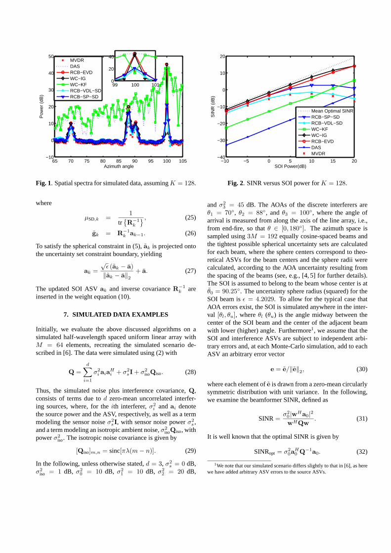
Fig. 1. Spatial spectra for simulated data, assumingK = 128.

where

µSD,k =1

tr{

R−1k

} , (25)

gk = R−1k ak−1. (26)

To satisfy the spherical constraint in (5),ak is projected ontothe uncertainty set constraint boundary, yielding

ak =

√ǫ (ak − a)

‖ak − a‖2+ a. (27)

The updated SOI ASVak and inverse covarianceR−1k are

inserted in the weight equation (10).

7. SIMULATED DATA EXAMPLES

Initially, we evaluate the above discussed algorithms on asimulated half-wavelength spaced uniform linear array withM = 64 elements, recreating the simulated scenario de-scribed in [6]. The data were simulated using (2) with

Q =d

∑

i=1

σ2i aia

Hi + σ2

sI+ σ2isoQiso. (28)

Thus, the simulated noise plus interference covariance,Q,consists of terms due tod zero-mean uncorrelated interfer-ing sources, where, for theith interferer,σ2

i andai denotethe source power and the ASV, respectively, as well as a termmodeling the sensor noiseσ2

sI, with sensor noise powerσ2s ,

and a term modeling an isotropic ambient noise,σ2isoQiso, with

powerσ2iso. The isotropic noise covariance is given by

[Qiso]m,n = sinc[πλ(m− n)]. (29)

In the following, unless otherwise stated,d = 3, σ2s = 0 dB,

σ2iso = 1 dB, σ2

0 = 10 dB, σ21 = 10 dB, σ2

2 = 20 dB,

−10 −5 0 5 10 15 20−40

−30

−20

−10

0

10

20

SOI Power(dB)

SIN

R (

dB)

Mean Optimal SINRRCB−SP−SDRCB−VDL−SDWC−KFWC−IGRCB−EVDDASMVDR

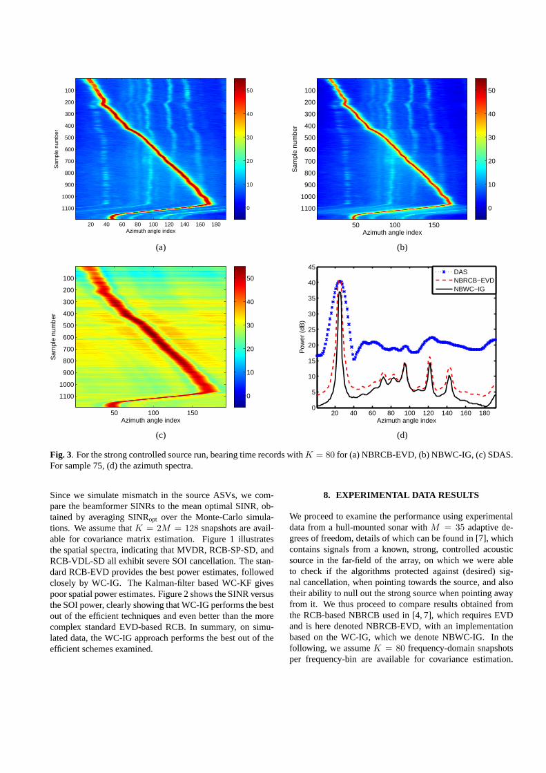
Fig. 2. SINR versus SOI power forK = 128.

andσ23 = 45 dB. The AOAs of the discrete interferers are

θ1 = 70◦, θ2 = 88◦, andθ3 = 100◦, where the angle ofarrival is measured from along the axis of the line array, i.e.,from end-fire, so thatθ ∈ [0, 180◦]. The azimuth space issampled using3M = 192 equally cosine-spaced beams andthe tightest possible spherical uncertainty sets are calculatedfor each beam, where the sphere centers correspond to theo-retical ASVs for the beam centers and the sphere radii werecalculated, according to the AOA uncertainty resulting fromthe spacing of the beams (see, e.g., [4, 5] for further details).The SOI is assumed to belong to the beam whose center is atθ0 = 90.25◦. The uncertainty sphere radius (squared) for theSOI beam isǫ = 4.2029. To allow for the typical case thatAOA errors exist, the SOI is simulated anywhere in the inter-val [θl, θu], whereθl (θu) is the angle midway between thecenter of the SOI beam and the center of the adjacent beamwith lower (higher) angle. Furthermore1, we assume that theSOI and interference ASVs are subject to independent arbi-trary errors and, at each Monte-Carlo simulation, add to eachASV an arbitrary error vector

e = e/‖e‖2, (30)

where each element ofe is drawn from a zero-mean circularlysymmetric distribution with unit variance. In the following,we examine the beamformer SINR, defined as

SINR=σ20 |wHa0|2wHQw

. (31)

It is well known that the optimal SINR is given by

SINRopt = σ20a

H0 Q−1a0. (32)

1We note that our simulated scenario differs slightly to that in [6], as herewe have added arbitrary ASV errors to the source ASVs.

Azimuth angle index

Sam

ple

num

ber

20 40 60 80 100 120 140 160 180

100

200

300

400

500

600

700

800

900

1000

1100 0

10

20

30

40

50

Azimuth angle index

Sam

ple

num

ber

50 100 150

100

200

300

400

500

600

700

800

900

1000

1100 0

10

20

30

40

50

(a) (b)

Azimuth angle index

Sam

ple

num

ber

50 100 150

100

200

300

400

500

600

700

800

900

1000

1100 0

10

20

30

40

50

20 40 60 80 100 120 140 160 1800

5

10

15

20

25

30

35

40

45

Azimuth angle index

Pow

er (

dB)

DASNBRCB−EVDNBWC−IG

(c) (d)

Fig. 3. For the strong controlled source run, bearing time recordswith K = 80 for (a) NBRCB-EVD, (b) NBWC-IG, (c) SDAS.For sample 75, (d) the azimuth spectra.

Since we simulate mismatch in the source ASVs, we com-pare the beamformer SINRs to the mean optimal SINR, ob-tained by averaging SINRopt over the Monte-Carlo simula-tions. We assume thatK = 2M = 128 snapshots are avail-able for covariance matrix estimation. Figure 1 illustratesthe spatial spectra, indicating that MVDR, RCB-SP-SD, andRCB-VDL-SD all exhibit severe SOI cancellation. The stan-dard RCB-EVD provides the best power estimates, followedclosely by WC-IG. The Kalman-filter based WC-KF givespoor spatial power estimates. Figure 2 shows the SINR versusthe SOI power, clearly showing that WC-IG performs the bestout of the efficient techniques and even better than the morecomplex standard EVD-based RCB. In summary, on simu-lated data, the WC-IG approach performs the best out of theefficient schemes examined.

8. EXPERIMENTAL DATA RESULTS

We proceed to examine the performance using experimentaldata from a hull-mounted sonar withM = 35 adaptive de-grees of freedom, details of which can be found in [7], whichcontains signals from a known, strong, controlled acousticsource in the far-field of the array, on which we were ableto check if the algorithms protected against (desired) sig-nal cancellation, when pointing towards the source, and alsotheir ability to null out the strong source when pointing awayfrom it. We thus proceed to compare results obtained fromthe RCB-based NBRCB used in [4, 7], which requires EVDand is here denoted NBRCB-EVD, with an implementationbased on the WC-IG, which we denote NBWC-IG. In thefollowing, we assumeK = 80 frequency-domain snapshotsper frequency-bin are available for covariance estimation.

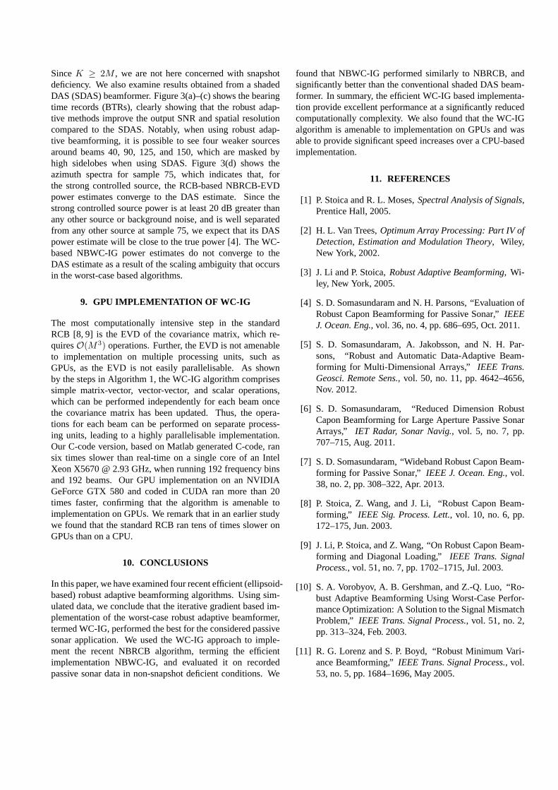
SinceK ≥ 2M , we are not here concerned with snapshotdeficiency. We also examine results obtained from a shadedDAS (SDAS) beamformer. Figure 3(a)–(c) shows the bearingtime records (BTRs), clearly showing that the robust adap-tive methods improve the output SNR and spatial resolutioncompared to the SDAS. Notably, when using robust adap-tive beamforming, it is possible to see four weaker sourcesaround beams 40, 90, 125, and 150, which are masked byhigh sidelobes when using SDAS. Figure 3(d) shows theazimuth spectra for sample 75, which indicates that, forthe strong controlled source, the RCB-based NBRCB-EVDpower estimates converge to the DAS estimate. Since thestrong controlled source power is at least 20 dB greater thanany other source or background noise, and is well separatedfrom any other source at sample 75, we expect that its DASpower estimate will be close to the true power [4]. The WC-based NBWC-IG power estimates do not converge to theDAS estimate as a result of the scaling ambiguity that occursin the worst-case based algorithms.

9. GPU IMPLEMENTATION OF WC-IG

The most computationally intensive step in the standardRCB [8, 9] is the EVD of the covariance matrix, which re-quiresO(M3) operations. Further, the EVD is not amenableto implementation on multiple processing units, such asGPUs, as the EVD is not easily parallelisable. As shownby the steps in Algorithm 1, the WC-IG algorithm comprisessimple matrix-vector, vector-vector, and scalar operations,which can be performed independently for each beam oncethe covariance matrix has been updated. Thus, the opera-tions for each beam can be performed on separate process-ing units, leading to a highly parallelisable implementation.Our C-code version, based on Matlab generated C-code, ransix times slower than real-time on a single core of an IntelXeon X5670 @ 2.93 GHz, when running 192 frequency binsand 192 beams. Our GPU implementation on an NVIDIAGeForce GTX 580 and coded in CUDA ran more than 20times faster, confirming that the algorithm is amenable toimplementation on GPUs. We remark that in an earlier studywe found that the standard RCB ran tens of times slower onGPUs than on a CPU.

10. CONCLUSIONS

In this paper, we have examined four recent efficient (ellipsoid-based) robust adaptive beamforming algorithms. Using sim-ulated data, we conclude that the iterative gradient based im-plementation of the worst-case robust adaptive beamformer,termed WC-IG, performed the best for the considered passivesonar application. We used the WC-IG approach to imple-ment the recent NBRCB algorithm, terming the efficientimplementation NBWC-IG, and evaluated it on recordedpassive sonar data in non-snapshot deficient conditions. We

found that NBWC-IG performed similarly to NBRCB, andsignificantly better than the conventional shaded DAS beam-former. In summary, the efficient WC-IG based implementa-tion provide excellent performance at a significantly reducedcomputationally complexity. We also found that the WC-IGalgorithm is amenable to implementation on GPUs and wasable to provide significant speed increases over a CPU-basedimplementation.

11. REFERENCES

[1] P. Stoica and R. L. Moses,Spectral Analysis of Signals,Prentice Hall, 2005.

[2] H. L. Van Trees,Optimum Array Processing: Part IV ofDetection, Estimation and Modulation Theory, Wiley,New York, 2002.

[3] J. Li and P. Stoica,Robust Adaptive Beamforming, Wi-ley, New York, 2005.

[4] S. D. Somasundaram and N. H. Parsons, “Evaluation ofRobust Capon Beamforming for Passive Sonar,”IEEEJ. Ocean. Eng., vol. 36, no. 4, pp. 686–695, Oct. 2011.

[5] S. D. Somasundaram, A. Jakobsson, and N. H. Par-sons, “Robust and Automatic Data-Adaptive Beam-forming for Multi-Dimensional Arrays,” IEEE Trans.Geosci. Remote Sens., vol. 50, no. 11, pp. 4642–4656,Nov. 2012.

[6] S. D. Somasundaram, “Reduced Dimension RobustCapon Beamforming for Large Aperture Passive SonarArrays,” IET Radar, Sonar Navig., vol. 5, no. 7, pp.707–715, Aug. 2011.

[7] S. D. Somasundaram, “Wideband Robust Capon Beam-forming for Passive Sonar,”IEEE J. Ocean. Eng., vol.38, no. 2, pp. 308–322, Apr. 2013.

[8] P. Stoica, Z. Wang, and J. Li, “Robust Capon Beam-forming,” IEEE Sig. Process. Lett., vol. 10, no. 6, pp.172–175, Jun. 2003.

[9] J. Li, P. Stoica, and Z. Wang, “On Robust Capon Beam-forming and Diagonal Loading,”IEEE Trans. SignalProcess., vol. 51, no. 7, pp. 1702–1715, Jul. 2003.

[10] S. A. Vorobyov, A. B. Gershman, and Z.-Q. Luo, “Ro-bust Adaptive Beamforming Using Worst-Case Perfor-mance Optimization: A Solution to the Signal MismatchProblem,” IEEE Trans. Signal Process., vol. 51, no. 2,pp. 313–324, Feb. 2003.

[11] R. G. Lorenz and S. P. Boyd, “Robust Minimum Vari-ance Beamforming,”IEEE Trans. Signal Process., vol.53, no. 5, pp. 1684–1696, May 2005.

[12] A. E.-Keyi, T. Kirubarajan, and A. B. Gershman, “Ro-bust Adaptive Beamforming Based on the Kalman Fil-ter,” IEEE Trans. Signal Process., vol. 53, no. 8, pp.3032–3041, Aug. 2005.

[13] A. Elnashar, “Efficient Implementation of Robust Adap-tive Beamforming Based on Worst-Case PerformanceOptimization,” IEEE Trans. Signal Process., vol. 2, no.4, pp. 381–393, Dec. 2008.

[14] A. Elnashar, S. M. Elnoubi, and H. A. El-Mikati, “Fur-ther Study on Robust Adaptive Beamforming with Op-timum Diagonal Loading,” IEEE Trans. AntennasPropag., vol. 54, no. 12, pp. 3647–3658, Dec. 2006.

[15] W. Zhang and S. Wu, “Low-Complexity Online Imple-mentation of a Robust Capon Beamformer,” inProc.Sensor Signal Processing for Defence, London, U.K.,Sep. 25-27 2012.