Computational Voting Theory - Computer Sciencexial/Files/dissertation_Lirong.pdf · Computational...
316
Computational Voting Theory: Game-Theoretic and Combinatorial Aspects by Lirong Xia Department of Computer Science Duke University Date: Approved: Vincent Conitzer, Supervisor J´ erˆomeLang Kamesh Munagala Ronald Parr Aleksandar Sasa Pekec Curtis R. Taylor Dissertation submitted in partial fulfillment of the requirements for the degree of Doctor of Philosophy in the Department of Computer Science in the Graduate School of Duke University 2011
Transcript of Computational Voting Theory - Computer Sciencexial/Files/dissertation_Lirong.pdf · Computational...
Computational Voting Theory:
Game-Theoretic and Combinatorial Aspects
by
Lirong Xia
Department of Computer ScienceDuke University
Date:
Approved:
Vincent Conitzer, Supervisor
Jerome Lang
Kamesh Munagala
Ronald Parr
Aleksandar Sasa Pekec
Curtis R. Taylor
Dissertation submitted in partial fulfillment of the requirements for the degree ofDoctor of Philosophy in the Department of Computer Science
in the Graduate School of Duke University2011

Abstract(Computer Science)
Computational Voting Theory:
Game-Theoretic and Combinatorial Aspects
by
Lirong Xia
Department of Computer ScienceDuke University
Date:
Approved:
Vincent Conitzer, Supervisor
Jerome Lang
Kamesh Munagala
Ronald Parr
Aleksandar Sasa Pekec
Curtis R. Taylor
An abstract of a dissertation submitted in partial fulfillment of the requirements forthe degree of Doctor of Philosophy in the Department of Computer Science
in the Graduate School of Duke University2011

Copyright c© 2011 by Lirong XiaAll rights reserved

Abstract
For at least two thousand years, voting has been used as one of the most effective
ways to aggregate people’s ordinal preferences. In the last 50 years, the rapid devel-
opment of Computer Science has revolutionize every aspect of the world, including
voting. This motivates us to study (1) conceptually, how computational think-
ing changes the traditional theory of voting, and (2) methodologically, how
to better use voting for preference/information aggregation with the help
of Computer Science.
My Ph.D. work seeks to investigate and foster the interplay between Computer
Science and Voting Theory. In this thesis, I will discuss two specific research di-
rections pursued in my Ph.D. work, one for each question asked above. The first
focuses on investigating how computational thinking affects the game-theoretic as-
pects of voting. More precisely, I will discuss the rationale and possibility of using
computational complexity to protect voting from a type of strategic behavior of the
voters, called manipulation. The second studies a voting setting called Combinatorial
Voting, where the set of alternatives is exponentially large and has a combinatorial
structure. I will focus on the design and analysis of novel voting rules for combina-
torial voting that balance computational efficiency and the expressivity of the voting
language, in light of some recent developments in Artificial Intelligence.
iv
To my dearest wife Jing. The past four years have been a very hard time for
both of us. Thank you for loving me, supporting me, encouraging me, and smiling
and crying for me since the very beginning. I will never forget the 61 days we spent
together in 2008, 108 days in 2009, 45 days in 2010, and 58 days by Aug. 11 in 2011.
v
Contents
Abstract iv
List of Tables xi
List of Figures xii
List of Abbreviations and Symbols xiv
Acknowledgements xvi
1 Introduction 1
1.1 Structure of This Dissertation . . . . . . . . . . . . . . . . . . . . . . 4
1.2 Computational Voting Theory . . . . . . . . . . . . . . . . . . . . . . 5
1.3 Node 2: Game-theoretic Aspects . . . . . . . . . . . . . . . . . . . . . 6
1.3.1 First Direction: Computational Complexity of Manipulation . 8
1.3.2 Second Direction: Equilibrium Outcomes in Voting Games . . 10
1.4 Node 3: Combinatorial Voting . . . . . . . . . . . . . . . . . . . . . . 11
1.4.1 Designing New Rules for Combinatorial Voting . . . . . . . . . 13
1.5 Node 4: Game-Theoretical Aspects of Combinatorial Voting . . . . . 16
1.6 Node 5: Work Excluded from My Dissertation . . . . . . . . . . . . . 18
1.6.1 My Other Work in Computational Voting Theory . . . . . . . 18
1.6.2 Combinatorial Prediction Markets . . . . . . . . . . . . . . . . 20
1.7 Summary . . . . . . . . . . . . . . . . . . . . . . . . . . . . . . . . . 21
vi
2 Preliminaries 22
2.1 Common Voting Rules . . . . . . . . . . . . . . . . . . . . . . . . . . 23
2.2 Axiomatic Properties for Voting Rules . . . . . . . . . . . . . . . . . 25
2.3 A Brief Overview of Computational Social Choice . . . . . . . . . . . 29
2.3.1 Major Topics in Computational Voting Theory . . . . . . . . . 29
2.3.2 Other Major Topics in Computational Social Choice . . . . . . 32
2.4 Summary . . . . . . . . . . . . . . . . . . . . . . . . . . . . . . . . . 35
3 Introduction to Game-theoretic Aspects of Voting 36
3.1 Coalitional Manipulation Problems . . . . . . . . . . . . . . . . . . . 36
3.2 Game Theory and Voting . . . . . . . . . . . . . . . . . . . . . . . . 42
3.3 Summary . . . . . . . . . . . . . . . . . . . . . . . . . . . . . . . . . 47
4 Computational Complexity of Unweighted Coalitional Manipula-tion 48
4.1 Manipulation for Maximin is NP-complete . . . . . . . . . . . . . . . 48
4.2 Manipulation for Ranked Pairs is NP-complete . . . . . . . . . . . . . 53
4.3 A Polynomial-time Algorithm for Manipulation for Bucklin . . . . . . 58
4.4 Summary . . . . . . . . . . . . . . . . . . . . . . . . . . . . . . . . . 60
5 Computing Manipulations is “Usually” Easy 62
5.1 Generalized Scoring Rules . . . . . . . . . . . . . . . . . . . . . . . . 63
5.2 Frequency of Manipulability for Generalized Scoring Rules . . . . . . 69
5.2.1 Conditions under Which Coalitional Manipulability is Rare . . 70
5.2.2 Conditions under which Coalitions of Manipulators are All-Powerful . . . . . . . . . . . . . . . . . . . . . . . . . . . . . . 73
5.2.3 All-Powerful Manipulators in Common Rules . . . . . . . . . . 79
5.3 An Axiomatic Characterization for Generalized Scoring Rules . . . . 83
5.3.1 Finite Local Consistency . . . . . . . . . . . . . . . . . . . . . 85
vii

5.3.2 Finite local consistency characterizes generalized scoring rules 86
5.4 A Scheduling Approach for Positional Scoring Rules . . . . . . . . . . 91
5.4.1 Algorithms for WCMd and COd . . . . . . . . . . . . . . . . . 95
5.4.2 Algorithm for WCM . . . . . . . . . . . . . . . . . . . . . . . 99
5.5 Algorithms for UCM and UCO . . . . . . . . . . . . . . . . . . . . . 103
5.5.1 On The Tightness of The Results . . . . . . . . . . . . . . . . 105
5.6 Summary . . . . . . . . . . . . . . . . . . . . . . . . . . . . . . . . . 107
6 Preventing Manipulation by Restricting Information 110
6.1 Framework for Manipulation with Partial Information . . . . . . . . . 113
6.2 Manipulation with Complete/No Information . . . . . . . . . . . . . 114
6.3 Manipulation with Partial Orders . . . . . . . . . . . . . . . . . . . . 118
6.4 Summary . . . . . . . . . . . . . . . . . . . . . . . . . . . . . . . . . 131
7 Stackelberg Voting Games 132
7.1 Stackelberg Voting Game . . . . . . . . . . . . . . . . . . . . . . . . . 135
7.2 Paradoxes . . . . . . . . . . . . . . . . . . . . . . . . . . . . . . . . . 136
7.3 Computing the Backward-Induction Outcome . . . . . . . . . . . . . 141
7.4 Experimental Results . . . . . . . . . . . . . . . . . . . . . . . . . . . 145
7.5 Summary . . . . . . . . . . . . . . . . . . . . . . . . . . . . . . . . . 148
8 Introduction to Combinatorial Voting 149
8.1 Multiple-Election Paradoxes . . . . . . . . . . . . . . . . . . . . . . . 153
8.2 CP-nets . . . . . . . . . . . . . . . . . . . . . . . . . . . . . . . . . . 155
8.3 Sequential Voting . . . . . . . . . . . . . . . . . . . . . . . . . . . . . 159
8.4 Summary . . . . . . . . . . . . . . . . . . . . . . . . . . . . . . . . . 165
9 A Framework for Aggregating CP-nets 166
9.1 Acyclic CP-nets Are Restrictive . . . . . . . . . . . . . . . . . . . . . 167
viii
9.2 H-Composition of Local Voting Rules . . . . . . . . . . . . . . . . . . 169
9.3 Local vs. Global Properties . . . . . . . . . . . . . . . . . . . . . . . . 173
9.4 Computing H-Schwartz Winners . . . . . . . . . . . . . . . . . . . . . 175
9.5 Summary . . . . . . . . . . . . . . . . . . . . . . . . . . . . . . . . . 180
10 A Maximum-Likelihood Approach 182
10.1 Maximum-Likelihood Approach to Voting in Unstructured Domains . 184
10.2 Multi-Issue Domain Noise Models . . . . . . . . . . . . . . . . . . . . 185
10.3 Characterizations of MLE correspondences . . . . . . . . . . . . . . . 188
10.4 Distance-Based Models . . . . . . . . . . . . . . . . . . . . . . . . . . 201
10.5 Summary . . . . . . . . . . . . . . . . . . . . . . . . . . . . . . . . . 211
11 Strategic Sequential Voting 213
11.1 Strategic Sequential Voting . . . . . . . . . . . . . . . . . . . . . . . . 219
11.1.1 Formal Definition . . . . . . . . . . . . . . . . . . . . . . . . . 219
11.1.2 Strategic Sequential Voting vs. Truthful Sequential Voting . . 223
11.1.3 A Second Interpretation of SSP . . . . . . . . . . . . . . . . . 224
11.1.4 The Winner is Sensitive to The Order over The Issues . . . . . 226
11.2 Minimax Satisfaction Index . . . . . . . . . . . . . . . . . . . . . . . 231
11.3 Multiple-Election Paradoxes for Strategic Sequential Voting . . . . . 232
11.4 Multiple-Election Paradoxes for SSP with Restrictions on Preferences 240
11.5 Summary . . . . . . . . . . . . . . . . . . . . . . . . . . . . . . . . . 251
12 Strategy-Proof Voting Rules over Restricted Domains 253
12.1 Conditional Rule Nets (CR-Nets) . . . . . . . . . . . . . . . . . . . . 255
12.2 Restricting Voters’ Preferences . . . . . . . . . . . . . . . . . . . . . . 257
12.3 Strategy-Proof Voting Rules in Lexicographic Preference Domains . . 260
12.4 Summary . . . . . . . . . . . . . . . . . . . . . . . . . . . . . . . . . 267
ix

13 Conclusion and Future Directions 269
13.1 Summary of Chapters . . . . . . . . . . . . . . . . . . . . . . . . . . 270
13.2 Future Directions . . . . . . . . . . . . . . . . . . . . . . . . . . . . . 273
13.2.1 Game-Theoretic Aspects . . . . . . . . . . . . . . . . . . . . . 274
13.2.2 Combinatorial Aspects . . . . . . . . . . . . . . . . . . . . . . 278
Bibliography 282
Biography 299
x

List of Tables
2.1 Some common voting rules and their axiomatic properties. . . . . . . 27
2.2 The doctrinal paradox. . . . . . . . . . . . . . . . . . . . . . . . . . . 34
3.1 Computational complexity of UCM for common voting rules. . . . . . 39
3.2 The prisoner’s dilemma. . . . . . . . . . . . . . . . . . . . . . . . . . 43
6.1 Computational complexity of the dominating manipulation problemswith partial orders, for common voting rules. . . . . . . . . . . . . . . 113
8.1 Comparing voting rules and languages for combinatorial voting. . . . 162
8.2 Local vs. global for sequential rules (Lang and Xia, 2009). . . . . . . 163
9.1 Local vs. global for H-compositions. . . . . . . . . . . . . . . . . . . . 175
11.1 The SSP winners for P 1 w.r.t. different orders over the issues. . . . . 227
11.2 From Pl to Pl1. . . . . . . . . . . . . . . . . . . . . . . . . . . . . . . 249
xi

List of Figures
1.1 Structure of my dissertation. . . . . . . . . . . . . . . . . . . . . . . . 4
1.2 Two directions in game-theoretic aspects of voting. . . . . . . . . . . 8
1.3 Two directions in combinatorial voting. . . . . . . . . . . . . . . . . . 13
1.4 Topics excluded from my dissertation. . . . . . . . . . . . . . . . . . . 18
2.1 The weighted majority graph of the profile define in Example 1.2.1. . 28
3.1 An extensive-form game. . . . . . . . . . . . . . . . . . . . . . . . . . 46
4.1 DP NM for Q1 x1 _ x2 _ x3. . . . . . . . . . . . . . . . . . . . . . . 54
5.1 An example schedule. The machines are idle in shaded areas. . . . . . 97
5.2 Conversion of an optimal schedule to a solution for WCMd. . . . . . . 98
6.1 F ~etc1,c2u. . . . . . . . . . . . . . . . . . . . . . . . . . . . . . . . . . . . 129
7.1 Simulation results for plurality and veto . . . . . . . . . . . . . . . . 147
8.1 A CP-net N and its induced partial order. . . . . . . . . . . . . . . . 157
8.2 The hypercube representation of the CP-net in Example 8.2.3. . . . . 158
9.1 Two votes and their induced graph. . . . . . . . . . . . . . . . . . . . 170
10.1 The noise model. . . . . . . . . . . . . . . . . . . . . . . . . . . . . . 185
10.2 The distance-based model πpq0,q1,q2q when the correct winner is 000. . 204
10.3 Distance-based threshold models. The weight of the bold edges isq ¡ 1
2; the weight of all other edges is 1
2. . . . . . . . . . . . . . . . . 204
11.1 A voting tree that is equivalent to the strategic sequential voting pro-cedure (p 3). 000 is the abbreviation for 010203, etc. . . . . . . . . . 223
xii

11.2 The majority graphs for p 2 and p 3. . . . . . . . . . . . . . . . . 227
xiii

List of Abbreviations and Symbols
Symbols
C tc1, . . . , cmu The set of alternatives (candidates).
P pV1, . . . , Vnq An n-profile.
m Number of alternatives.
n Number of voters.
n1 Number of manipulators.
r A voting rule.
rc A voting correspondence.
Additional Symbols for Combinatorial Voting
p Number of issues (characteristics).
Xi The ith issue.
Di The ith local domains.
X D1 Dp A multi-issue domain composed of p issues.
ri A local rule over Di.
SeqOpr1, . . . , rpq The sequential composition of local rules r1, . . . , rp.
L Admissible conditional preference set (Definition 12.2.1).
CPnetspLq The set of all CP-nets consistent with L (Definition 12.2.2).
PrefpLq The set of all linear orders that are consistent with L (Defini-tion 12.2.2).
LDpLq The lexicographic preference domain (Definition 12.2.2).
xiv

Abbreviations
WCM Weighted coalitional manipulation.
UCM Unweighted coalitional manipulation.
UCO Unweighted coalitional optimization.
COd Coalitional optimization with divisible votes.
GSR Generalized scoring rules.
NE Nash equilibrium.
SPNE Subgame-perfect Nash equilibrium.
xv

Acknowledgements
I am deeply indebted to my supervisor Vincent Conitzer. Needless to say, everyone
who knows him knows how great he is. He is a wonderful researcher to work with,
a great friend to chat with, and of course, a superb supervisor who always gives
me very helpful advises and suggestions. He has always been extremely supportive,
patient, and, mostly amazingly, always available WHENEVER I need help. From
him I learned a lot: how to do high-quality research, how to manage time as a junior
faculty member, and even how to speak English, etc. He makes me firmly believe
that coming to Duke is the best choice for my Ph.D. study.
I am also deeply grateful to Jerome Lang, who is effectively my secondary su-
pervisor. Jerome has been a frequent collaborator of me and has been helping me
so much in research, job search, and many other things ever since before I came to
Duke. Besides Vince and Jerome, I am very fortunate and proud to have Ron Parr,
Kamesh Munagala, Sasa Pekec, and Curt Taylor in my Ph.D. committee. Thank
you for your advises, feedback, and support in my research as well as job search.
Also I should thank Toby Walsh for very insightful and quick feedback on my dis-
sertation. Special thanks to my supervisor Mingsheng Ying when I was in China,
who introduced me to the field of Computational Social Choice, and has been very
considerate and supportive. In addition to Vince and Jerome, I am also extremely
thankful to Lane Hemaspaandra, Dave Pennock and Toby Walsh for their support
in my job search, especially for writing and submitting recommendation letters so
xvi
timely. Many thanks to all other friends who have given me very useful feedback on
my research statements and helped me in my job search, including Atila Abdulka-
diroglu, Itai Ashlagi, Yiling Chen, Edith Elkind, Maria Gini, Mingyu Guo, Edith
Hemaspaandra, Shaili Jain, Dima Korzhyk, Nicolas Lambert, Michel Le Breton,
Christopher Painter-Wakefield, David Parkes, and Tuomas Sandholm.
I had a very pleasant and rewarding summer intern experience at Yahoo! Research
New York in 2010. It was my great pleasure to work with and learn from many
excellent researchers in the Microeconomics group there, including Dave Pennock,
Dan Reeves, Sebastien Lahaie, and Giro Cavallo. During my Ph.D. study, I have
been very fortunate to work and publish with many fantastic researchers, including
Sayan Bhattacharya, Yann Chevaleyre, Vincent Conitzer, Tao Jiang, Jerome Lang,
Lan Liu, Nicolas Maudet, Jerome Monnot, Kamesh Munagala, Nina Narodytska,
Dave Pennock, Ariel Procaccia, Matthew Rognlie, Jeff Rosenschein, Toby Walsh,
Jing Xiao, and Michael Zuckerman. I also thank a James B. Duke Fellowship and
my supervisor Vince Conitzer’s NSF CAREER 0953756 and IIS- 0812113, and an
Alfred P. Sloan fellowship for support.
Last but of course not least I want to thank my parents, to whom I owe the most
for their selfless love and support.
xvii
1
Introduction
People hold different opinions and preferences over almost everything. Yet in many
situations a common decision must be made. For example, sometimes people need
to select a leader, or decide whether or not to provide a public good such as national
defense. The best-known way to achieve these goals is by voting, which has been a
critical component of democracy since ancient time. As early as around 350 B.C.,
Plato (424/423 B.C.–348/347 B.C.), in spite of being famous for his objection against
democracy, proposed several multi-stage voting processes to elect the “guardians” of
the law and officeholders, etc., in his unfinished book “The Law”. Obviously Plato
was not the first person who thought about voting. In fact, Socrates (469 B.C.–
399 B.C.), Plato’s teacher, was sentenced to death by a majority voting. Plato
thus had good reasons to object to democracy. After Plato, the first well-known
voting system that is not based on majority voting was proposed by Ramon Llull
(1232–1315). Then, the systematic study of the theory of voting prospered with the
French Revolution in the 18th century. During that time, two of the most famous
philosophers who made significant contributions to the theory of voting are Marie
Jean Antoine Nicolas de Caritat, marquis de Condorcet (1743–1794, also known as
1

Nicolas de Condorcet, who proposed the Condorcet criterion), and Jean-Charles,
chevalier de Borda (1733–1799, who proposed the Borda voting rule). More recently,
Kenneth Arrow (a co-recipient of the Nobel Memorial Prize in Economics in 1972)
showed that it is impossible to design a voting rule that satisfies some very natural
properties (Arrow, 1950). This seminal work is thus named Arrow’s impossibility
theorem, and is broadly regarded as the beginning of modern Social Choice Theory,
which is an active research direction in Economics.
In recent years, rapid developments in computers and networks have brought big
changes to human society. Computers not only have helped us solve problems faster,
but also have brought revolutions to the ideology of the human society. For exam-
ple, the ultimate goal of Artificial Intelligence (AI) is to build computers that are as
“intelligent” as, if not more intelligent than, human beings. These changes have led
to many new interdisciplinary areas. In particular, the interdisciplinary area lying
in the intersection of Computer Science and Economics has attracted huge atten-
tion, partly due to the emerging electronic commerce of the Internet era. One place
where Computer Science meets Economics is the new subarea of AI called Multi-
Agent Systems, which studies interactions and collaborations in systems that consist
of multiple intelligent agents (Wooldridge, 2009). Similar as for human beings, vot-
ing could help intelligent agents to make a joint decision in many situations. For
example, in the system developed by Ephrati and Rosenschein (1991), agents use
voting to decide the next step in their joint plan. There are also many applications
of voting in electronic commerce, for example, Ghosh et al. (1999) proposed to use
voting to help build recommendation systems; Pennock et al. (2000) adopted the
core method in traditional Voting Theory—the axiomatic approach—to analyze col-
laborative filtering algorithms in recommendation systems; and Dwork et al. (2001)
proposed to treat web-search engines as agents, and use voting to decide the best
matching website.
2
In many new applications of voting, we encounter an extremely large number
of alternatives or an overwhelming amount of information, which leads to signifi-
cant computational challenges. To handle these situations, we need to design faster
algorithms or build faster computers. On the other hand, higher computational ca-
pability makes it easier for voters to figure out beneficial strategic behavior, which
might lead to undesirable outcomes. In order to reap the benefits of these potential
applications and overcome the emerging problems, we need to develop new algo-
rithms and methodologies. A burgeoning area—Computational Social Choice—aims
to address problems in computational aspects of information/preference representa-
tion and aggregation in multi-agent scenarios (Chevaleyre et al., 2007).
A first question that should be asked is: why it is voting that people or intel-
ligent agents should want to use to aggregate their preferences? Certainly in some
situations people use other mechanisms. For example, sometimes auctions are used
to determine an allocation of resources or tasks. A key feature in the situations
where people or agents use voting is that they only have, or are limited to express,
ordinal preferences, in contrast to cardinal preferences measured by real numbers
that represent utilities and allow for monetary transfers. In this dissertation, I put
aside the discussion of many important topics, including the comparison between
voting and other mechanisms, cardinal vs. ordinal preferences, rationale behind the
utility theory, etc. An interested reader may refer to Conitzer (2010) for discus-
sions on such topics. Instead, I will focus on the situations where voting is used.
It should be kept in mind that voting is a good option for preference/information
aggregation in many, but not all situations. My research seeks to investigate and
foster the interplay between Computer Science and Voting Theory. In particular, my
research focuses the conceptual and methodological aspects of the interplay: (1) how
computational thinking (Wing, 2006) changes the traditional voting theory
conceptually, and (2) methodologically how can we better use voting for
3
preference/information aggregation with the help of Computer Science.
1.1 Structure of This Dissertation
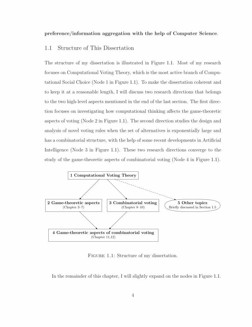
The structure of my dissertation is illustrated in Figure 1.1. Most of my research
focuses on Computational Voting Theory, which is the most active branch of Compu-
tational Social Choice (Node 1 in Figure 1.1). To make the dissertation coherent and
to keep it at a reasonable length, I will discuss two research directions that belongs
to the two high-level aspects mentioned in the end of the last section. The first direc-
tion focuses on investigating how computational thinking affects the game-theoretic
aspects of voting (Node 2 in Figure 1.1). The second direction studies the design and
analysis of novel voting rules when the set of alternatives is exponentially large and
has a combinatorial structure, with the help of some recent developments in Artificial
Intelligence (Node 3 in Figure 1.1). These two research directions converge to the
study of the game-theoretic aspects of combinatorial voting (Node 4 in Figure 1.1).
1 Computational Voting Theory
2 Game-theoretic aspects(Chapter 3–7)
3 Combinatorial voting(Chapter 8–10)
4 Game-theoretic aspects of combinatorial voting(Chapter 11,12)
5 Other topicsBriefly discussed in Section 1.5
Figure 1.1: Structure of my dissertation.
In the remainder of this chapter, I will slightly expand on the nodes in Figure 1.1.
4

1.2 Computational Voting Theory
Computational Voting Theory, which studies computational issues in voting, is the
most active branch of Computational Social choice. Throughout the dissertation, a
vote is a linear order1 over the set of alternatives (candidates), we ask each voter
(agents) to cast one vote. These votes constitute a profile. Then, we apply a voting
rule to the profile to determine the winning alternative (the winner).
Example 1.2.1. Suppose three candidates Clinton, Obama, McCain are competing
for a presidential position. We use the plurality rule to select the winner. That is, the
candidate who is ranked at the top the most time in the votes wins, and suppose ties
are broken alphabetically. Suppose there are five voters whose votes are as follows:
Voter 1 : Clinton¡Obama¡McCainVoter 2,3: Obama¡McCain¡ClintonVoter 4,5: McCain¡Clinton¡Obama
Then, the winner is McCain, because he is ranked in the top position for two times
(tied with Obama), and the tie is broken in favor of McCain.
The formal definition of voting systems and some popular voting rules can be
found in Chapter 2. In Computational Voting Theory, researchers have extensively
investigated at least the following questions.
• How can we compute the winner or ranking more efficiently?
• How can we communicate and elicit voters’ preferences more efficiently?
• How can we use computational complexity to protect elections from bribery
and control?
1 However, see Pini et al. (2007), for a discussion of voting where preferences over the candidatesare represented by a partial order.
5
• How can we prevent voters from misreporting their preferences?
• How can we analyze voters’ incentive and strategic behavior?
• How can we design novel voting rules when the set of alternatives has a com-
binatorial structure, and is exponentially large?
Nodes 2–4 correspond to the last three questions. More detailed discussions as well
as references can be found in Chapter 2.
1.3 Node 2: Game-theoretic Aspects
An important yet always implicit assumption when most popular voting rules were
designed is that all voters report their preferences truthfully. However, in many
real world voting systems, a voter may well lie to make herself better off. This
phenomenon is call a manipulation. For example, let us recall Example 1.2.1, and
suppose that the votes described in the example are the voters’ true preferences. We
have already seen that if all five voters report truthfully, then McCain is the win-
ner. However, if the first voter reports that her vote is Obama¡Clinton¡McCain,
while the other voters all report truthfully, then Obama is the winner. Note that
the first voter prefers Obama to MaCain, which means that she has an incentive
to misreport her preferences to make herself better off. This kind of strategic be-
havior makes the outcome of the voting process unpredictable, and can sometimes
hurt the voters, including the manipulators themselves, when there is more than one
manipulator. Therefore, it is important to investigate the strategic behavior of the
voters. This falls under Game Theory (Fudenberg and Tirole, 1991). First of all, it
would be great if we can use a voting rule for which there is never any opportunity
for manipulation, i.e., a strategy-proof voting rule. This objective might seem to
be too ambitious at first glance, but in fact, there are many strategy-proof mecha-
nisms in other settings where voters are allowed to express their cardinal preferences,
6

their preferences are quasi-linear, and monetary transfers are allowed. For example,
the well-known VCG mechanisms are strategy-proof (Vickrey, 1961; Clarke, 1971;
Groves, 1973). Unfortunately, in voting settings where no monetary transfers are
allowed, due to the celebrated Gibbard-Satterthwaite theorem (Gibbard, 1973; Sat-
terthwaite, 1975), when there are three or more alternatives, no strategy-proof voting
rule satisfies the following two desired properties: (1) non-imposition (i.e., each al-
ternative wins for some profile) and (2) non-dictatorship (i.e., there is no dictator, a
voter whose first-ranked alternative is always the winner). To circumvent this very
negative result, economists have proposed to restrict the domain of preferences to
obtain strategy-proofness. That is, we assume that voters’ preferences always lie in a
restricted set of linear orders. One example of such a class is the set of single-peaked
preferences (Black, 1948). For single-peaked preferences, desirable strategy-proof
rules exist, such as the median rule (Moulin, 1980). More details can be found in
Chapter 12, where I will discuss our own results along this line as well.
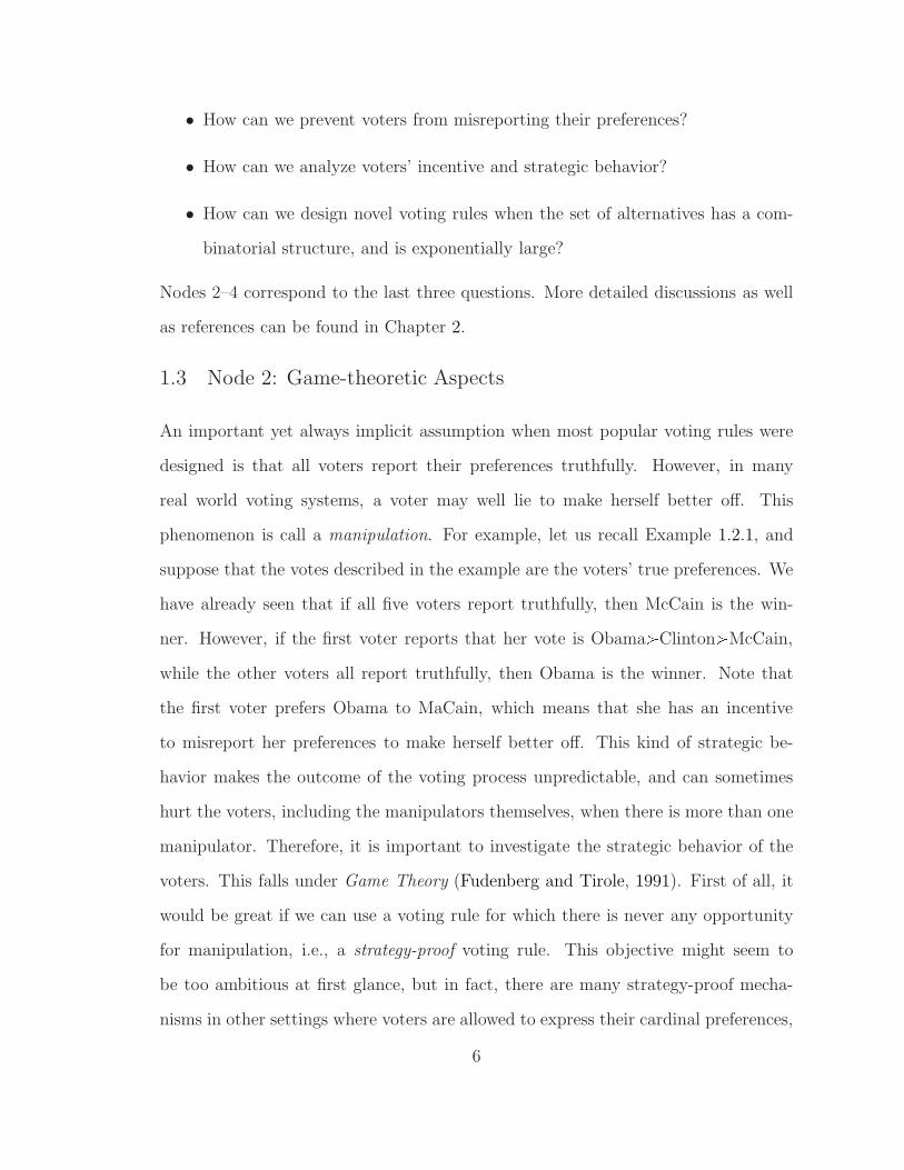
Besides this, my research on the game-theoretic aspects of Voting Theory di-
verges into two directions, illustrated in Figure 1.1. The first direction (the left
branch) focuses on exploring the idea of using computational complexity to prevent
manipulation. The second direction (the right branch) focuses on analyzing the
equilibrium outcome in a type of voting games.
7
Manipulation is inevitable(Gibbard-Satterthwaite Theorem)
Yes(Chapter 4)
No(Chapter 5)
Information constraints (Chapter 6)Domain restrictions (Chapter 12)
May lead to very undesirableoutcomes (Chapter 7,11)
Seems not very often(experiments in Chapter 7)
2 Game-theoretic aspects
Can we use computational complexityas a barrier against manipulation?
Is it a strong barrier?
Other barriers?
Why prevent manipulations?
How often?
Figure 1.2: Two directions in game-theoretic aspects of voting.
1.3.1 First Direction: Computational Complexity of Manipulation
Even though a manipulation is guaranteed to exist, if we can prove that finding a
manipulation is computationally hard for some common voting rules, then a ma-
nipulation might not occur simply because the manipulator(s) cannot find it in a
reasonable amount of time, or it is computationally too costly to do so. This idea
was first explored by Bartholdi et al. (1989a), which, together with Bartholdi et al.
(1989b, 1992), have been broadly considered the starting point of Computational
Social Choice. After that, a number of results have been obtained on the computa-
tional complexity of manipulation in various settings. See Faliszewski et al. (2010b);
Faliszewski and Procaccia (2010) for recent surveys. More details will also be given
in Chapter 4.
8
Chapter 4 focuses on the most natural setting where voters are equally weighted,
and there are multiple manipulators who want to cast their votes collaboratively to
make a favored alternative win. I will show that for some common voting rules,
finding a manipulation is NP-hard, while for some other voting rules, there exist
polynomial-time algorithms to find a manipulation. Therefore, at least for some
common voting rules, the answer to the question “Can we use computational com-
plexity as a barrier against manipulation?” is “Yes”. This answer is quite positive,
because it implies that at least for these voting rules, even if the potential manipula-
tors use the fastest computer in the world, they are unlikely to find an algorithm that
can always tell them the answer quickly even for large instances (assuming P NP).
Consequently, these potential manipulators might have less incentive to misreport
their preferences.
Proving the NP-hardness of finding a manipulation is only a first step. Even
though it is NP-hard to find a manipulation, the manipulators may still not always
report their true preferences. For example, they can certainly run a heuristic algo-
rithm for a certain amount of time, say one minute, and if the algorithm returns
a successful manipulation, then they will cast the votes returned by the algorithm;
otherwise, if the algorithm fails to compute an answer in one minute, they may
then report their true preferences. Technically, this problem is due to the fact that
NP-hardness is a worst-case concept. Therefore, it is natural to ask, informally,
whether manipulations are computationally hard to find in “most” cases. Some pre-
vious work gave partial answers to this question. Again, more details and discussion
can be found in Faliszewski et al. (2010b); Faliszewski and Procaccia (2010) and/or
Chapter 4. We will see in Chapter 5 that, for a very general class of voting rules
called generalized scoring rules, which include many common voting rules, the cases
where manipulations are hard to find are exceptions rather than the rule. There-
fore, computational complexity does not seem to be a very strong barrier against
9

strategic behavior, so that we need to seek other barriers. For example, we may
try to limit the manipulators’ information about the preferences of the other voters
(Chapter 6), or only allow the voters to pick a vote from a restricted set of linear
orders (Chapter 12).2
1.3.2 Second Direction: Equilibrium Outcomes in Voting Games
In fact, the very first question that should be asked is, is it ever desirable to prevent
the voters’ strategic behavior? After all, the ultimate objective of voting is to select
a “good” alternative. So if somehow the strategic behavior of the voters leads to the
same, or an even better, outcome, then there is no reason to even try to prevent the
voters from being strategic. Moreover, in such cases, maybe the strategic behavior
should actually be encouraged! Surprisingly, this question was not answered before.
To analyze the outcome when voters are strategic, the most natural way is to use
Game Theory to model the voting process as a game, and then focus on the winner in
the outcome of the game in terms of some solution concept, e.g., Nash equilibrium.3
However, in general a voting game has too many (Nash) equilibria. This makes it
very hard to draw any useful conclusions on the impact of strategic behavior on the
outcome of voting.
In Chapter 7, we study a type of voting games where voters cast their votes one
after another sequentially. We call such games Stackelberg voting games. We will fo-
cus on a finer solution concept called subgame-perfect Nash equilibrium. Fortunately,
in any Stackelberg voting game, the outcome is unique in all subgame-perfect Nash
equilibria. One might expect that the strategic behavior would sometimes harm the
voters, but there are two main difficulties in drawing such a conclusion, which come
2 As mentioned earlier, this idea has been approached mainly by economists. I will further exploreit in the setting of combinatorial voting.
3 In general simultaneous-move voting games, a Nash equilibrium is a profile where no voter canbenefit from casting a different vote. The formal definition of voting games, Nash equilibrium, andits refinement subgame-perfect Nash equilibrium can be found in Chapter 7.
10
from the following two natural questions.
1. To what extent can the strategic behavior harm the voters? The main difficulty
here is that voting aims at aggregating voters’ ordinal preferences, which means
that generally it is nontrivial to measure how good/bad an alternative is.4
2. How often does the strategic behavior harm the voters?
Chapter 7 answers the above two questions. The first question is answered by show-
ing some paradoxes, which state that sometimes the (unique) equilibrium winner is
ranked in extremely low positions in almost all voters’ true preferences. Without
doubt this is an extremely undesirable outcome. Therefore, these paradoxes illus-
trate the cost of strategic behavior of the voters, and suggest that at least in some
cases, strategic behavior should be prevented. The second question is partly an-
swered by simulations. Surprisingly, for most common voting rules, the winner in
the equilibrium outcome is slightly “better” for the voters on average, compared to
the winner when they vote truthfully.
1.4 Node 3: Combinatorial Voting
So far we have been discussing voting over unstructured sets of alternatives. In many
real-life situations, there are multiple issues (attributes, or characteristics), and each
alternative can be uniquely characterized by a vector of the values these issues take.
Such settings are called combinatorial voting (or voting in combinatorial domain).
For instance, when agents vote to select a president and a treasurer, each position
corresponds to an issue whose value corresponds to the person selected to hold the
4 This is in sharp contrast to the settings where there is a well-defined social welfare function,especially in the settings where the agents have quasilinear utility functions, and are allowed toexpress their cardinal preferences, for example in auctions. In those situations, the cost of strategicbehavior can be measured by the price of anarchy (Koutsoupias and Papadimitriou, 1999), that is,the ratio of the optimal social welfare over the worst social welfare in equilibrium outcomes.
11

position. In combinatorial voting, selecting a winner amounts to making a public
choice for each of the issues. The main difficulty resides in the exponentially large
number of alternatives. Therefore, it is computationally impractical to directly apply
a common voting rule designed for unstructured sets of alternatives in the setting of
combinatorial voting.5 For combinatorial voting, we need to design new voting rules
that are computationally tractable.
In the literature, researchers in Economics and Political Science have extensively
studied voting processes where the agents vote over issues separately in parallel. This
method works well when agents’ preferences over one issue do not depend on any
other issues. However, in general agents’ preferences over one issue may depend on
the value of other issues. For example, if a Democrat is selected to be the president,
then a voter may prefer selecting a Republican to be the treasurer; but if a Republican
is selected to be the president, then the voter may prefer selecting a Democrat to be
the treasurer. There are two main challenges for combinatorial voting: Language-
wise we need a more natural way for the agents to truthfully report their preferences.
Methodology-wise we also need a more general theory of computational tractable
combinatorial voting.
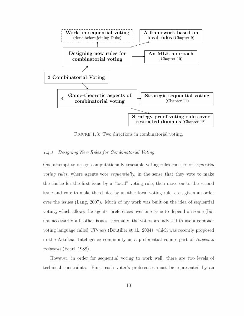
My research in combinatorial voting can be roughly categorized into two direc-
tions, illustrated in Figure 1.3. The first direction focuses on designing computation-
ally tractable voting rules for combinatorial voting. The second direction (Node 4 in
Figure 1.1) focuses on game-theoretic aspects of combinatorial voting, where we aim
at analyzing and preventing voters’ strategic behavior in combinatorial voting.
5 Some voting rules that only use a very small portion of the voters preferences to select thewinner, for example the plurality rule, do not have significant computational issues when they areused in combinatorial voting. However, in general these rules will not select a “good” outcome incombinatorial voting. More discussions will be given in Chapter 8.
12
3 Combinatorial Voting
Designing new rules forcombinatorial voting
A framework based onlocal rules (Chapter 9)
An MLE approach(Chapter 10)
Strategy-proof voting rules overrestricted domains (Chapter 12)
4Game-theoretic aspects of
combinatorial votingStrategic sequential voting
(Chapter 11)
Work on sequential voting(done before joining Duke)
Figure 1.3: Two directions in combinatorial voting.
1.4.1 Designing New Rules for Combinatorial Voting
One attempt to design computationally tractable voting rules consists of sequential
voting rules, where agents vote sequentially, in the sense that they vote to make
the choice for the first issue by a “local” voting rule, then move on to the second
issue and vote to make the choice by another local voting rule, etc., given an order
over the issues (Lang, 2007). Much of my work was built on the idea of sequential
voting, which allows the agents’ preferences over one issue to depend on some (but
not necessarily all) other issues. Formally, the voters are advised to use a compact
voting language called CP-nets (Boutilier et al., 2004), which was recently proposed
in the Artificial Intelligence community as a preferential counterpart of Bayesian
networks (Pearl, 1988).
However, in order for sequential voting to work well, there are two levels of
technical constraints. First, each voter’s preferences must be represented by an
13

acyclic CP-net. In other words, for each voter, there exists at least one linear ordering
over the issues, such that the voter’s preferences over later issues in this order only
depend on the values of all previous issues. That is, the voter’s preferences are
compatible with that ordering over issues. The second is that all voters’ preferences
must be compatible with a common (linear) ordering over the issues. For example,
consider a combinatorial voting setting where there are two issues: an issue for
“main dish”, which can be either fish or beef, and another issue for “wine”, which
can be either red wine or white wine. The two constraints state that there exists
an ordering over the two issues, w.l.o.g. main dish¡wine, with which all voters’
preferences are compatible. That is, each voter’ preferences over wine depends on the
value of main dish. From a high-level point of view, these two constraints imply that
sequential voting rules have high computational efficiency, but the voting language
(i.e., acyclic CP-nets that are compatible with a common ordering over issues) is
too restrictive. On the other hand, common voting rules designed for unstructured
sets of alternatives have low computational efficiency in the setting of combinatorial
voting, but the voters have more flexibility in expressing their preferences.
Designing a good voting rule with high computational efficiency and a fully ex-
pressive language seems to be a mission impossible. Therefore, my work in com-
binatorial voting aims to design voting rules that tradeoff computational efficiency
and expressiveness of the voting language. We will start designing such voting rules
by assuming all voters vote truthfully (Chapter 9, 10). Complications caused by
the strategic behavior of the voters will be examined later (Chapter 11, 12). In
Chapter 9, we will see a framework that first considers a directed graph over all
alternatives by applying local voting rules, then uses a choice set function to select
the winner from this graph. This framework allows a voter to use any CP-net (even
an acyclic one) to represent her preferences. We will also see that whether or not
the voting rule defined by this framework satisfies some desired properties for voting
14
rules, e.g., anonymity, neutrality, etc., depends on both the choice set function and
whether the local voting rules satisfy these properties. In general, computing the
winners in this framework is hard. However, we will see an algorithm that could save
significant amounts of time when the (possibly cyclic) CP-nets that represent voters’
preferences share some common structure.
Chapter 10 takes a different approach towards defining new rules for combina-
torial voting. Suppose there is a “correct” winner and the voters’ preferences are
noisy perceptions of it. If we have a probabilistic model that generates voters’ pref-
erences given the “correct” winner, and a probability distribution for an alternative
to be the “correct” winner, then having seen the voters vote, we can compute the
posterior probability for each alternative to be the “correct” winner via standard
Bayesian reasoning. In other words, the voting rule defined by this process can be
viewed as the maximum likelihood estimator (MLE) of the probabilistic model. This
idea was actually introduced two hundred years ago by Condorcet (1785) to design
a voting rule for unstructured sets of alternatives. The main question is, how should
we define the probabilistic model? In Chapter 10, we will see a natural probabilistic
model for sets of alternatives composed of binary issues, called distance-based noise
models, where the conditional probability given the “correct” winner is decomposed
into local distributions, one for each issue i. More precisely, the local distribution
over any issue i under some setting of the other issues depends only on the Hamming
distance from this setting to the restriction of the “correct” winner to the issues other
than i. Some results on the computational complexity of winner computation will
be presented, followed by discussions about the relation between the MLE approach
and sequential voting rules.
15

1.5 Node 4: Game-Theoretical Aspects of Combinatorial Voting
The formulation of a voting game largely depends on the voting rule used in the
voting process. As I argued in the last section, in combinatorial voting it is generally
computationally costly to use common voting rules designed for unstructured sets
of alternatives. Therefore, the arguments and results in Section 1.3, which were
made for common voting rules designed for unstructured sets of alternatives, do
not directly apply to combinatorial voting. Since sequential voting is one of the
most natural approaches in combinatorial voting, this suggests to study a voting
game where voters cast votes strategically on one issue after another, following some
ordering over the issues. Indeed, strategic voting is arguably more likely in such a
sequential game than in “one shot” voting. We call this type of voting games strategic
sequential voting, which is the main topic of Chapter 11.6 Compared to (truthful)
sequential voting mentioned in the previous subsection, for strategic sequential voting
the focus is on different aspects. In truthful sequential voting, a major concern is
how expressive the voting language is. In strategic sequential voting, however, the
expressivity of the voting language is not the most important issue. Instead, what
really matters is how a strategic voter’s preferences and knowledge about the other
voters’ preferences determine her behavior in the voting game, and thus influence the
outcome of the game. Therefore, in the game-theoretic part on combinatorial voting,
we are interested in the following two questions. The first question is exactly the
same as question 1 asked in Section 1.3.2, but here it is asked for strategic sequential
voting.
1. To what extent can the strategic behavior harm the voters in strategic sequen-
6 We note that strategic sequential voting is different from the Stackelberg voting games mentionedin Section 1.3.2. In Stackelberg voting games voters cast their votes one after another, while instrategic sequential voting, voters cast votes simultaneously on individual issues, one issue afteranother.
16
tial voting?
2. If the strategic behavior of the voters can harm the voters badly, how can we
prevent it?
The first question is answered by three types of multiple-election paradoxes: there
exists a profile for which (1) the winner under strategic sequential voting is ranked
nearly at the bottom in all voters’ true preferences, (2) the winner is Pareto-dominated
by almost every other alternative, and as a consequence, (3) the winner is an almost
Condorcet loser.7 Even worse, changing the ordering over the issues on which the
voters vote cannot completely prevent these paradoxes. Hence, the outcome of strate-
gic sequential voting can be extremely undesirable to all voters. Similar paradoxes
have been shown for other models of behavior in combinatorial voting in the liter-
ature (Scarsini, 1998; Brams et al., 1998), but as far as we know, we were the first
to discover these paradoxes in a strategic environment, to illustrate the cost of the
strategic behavior of the voters. See Chapter 11 for more references and discussion.
One approach to addressing the concern raised by the second question is restrict-
ing the voters’ preferences. We will see in Chapter 11 that by restricting the voters’
preferences to be separable or lexicographic, all three types of multiple-election para-
doxes mentioned earlier disappear. In fact, by putting more constraints on the voters’
preferences, we can obtain strategy-proof sequential voting rules for combinatorial
voting. We can further show that if the domain restriction satisfies some mild condi-
tions, then a voting rule is strategy-proof if and only if it is a sequential voting rule,
where each local rule is strategy-proof over its respective local domain. This will be
discussed in Chapter 12.
7 The definitions for Pareto-domination and Condorcet loser will be found in Chapter 11.
17

1.6 Node 5: Work Excluded from My Dissertation
During my Ph.D. studies, I also have worked on some other important topics in
preference/information representation and aggregation. These works will not be
discussed in detail in the dissertation due to considerations of length and coherence
of the dissertation. In this section, I will briefly describe these works, illustrated in
Figure 1.4. An interested reader may also refer to Xia (2010).
5 Other work excluded from the thesis
Possible/Necessary winners(Xia and Conitzer, 2008, 2011a;
Chevaleyre et al., 2010b; Xia et al., 2011)
MLE approach(Conitzer et al., 2009;
Xia and Conitzer 2011b)
Compilation complexity(Xia and Conitzer, 2010)
An efficient pricing algorithm(Xia and Pennock, 2011)
Pricing with Bayesian Networks(Pennock and Xia, 2011)
Combinatorial prediction markets
Computational voting theory
Figure 1.4: Topics excluded from my dissertation.
1.6.1 My Other Work in Computational Voting Theory
In addition to the topics discussed in Section 1.3, 1.4, and 1.5, I have also worked on
the following three topics.
• Computing possible/necessary winners. In practice, we may not need to
know the voters’ full preferences to compute the winner. That is, information
elicited at an early stage might suffice to conclude who the winner is. For this
purpose, it is important to know the answers to the following two computa-
tional questions when only part of the voters’ preferences are elicited: (1) Is it
18

still possible for a given alternative to win? (2) Has the winner already been
determined, so that we may terminate the elicitation process and announce the
winner? These two problems are known as the possible/necessary winner prob-
lems, respectively (Conitzer and Sandholm, 2002; Konczak and Lang, 2005). I
investigated the computational complexity of these possible/necessary winner
problems for many common voting rules (Xia and Conitzer, 2008a, 2011a), as
well as in the special case where the alternatives do not arrive at the same
time (Chevaleyre et al., 2010b,a; Xia et al., 2011).
• Compilation complexity. One closely related topic to possible/neccessary
winner determination is the compilation complexity of common voting rules.
Here the agents do not arrive at the same time, and we are asked in the mid-
dle of the election, what is the lowest number of bits required to store enough
information about the votes cast so far to determine the winer (Chevaleyre
et al., 2009). In recent work (Xia and Conitzer, 2010a), we proved asymp-
totically matching upper and lower bounds on the compilation complexity for
many common voting rules. We also devised polynomial-time algorithms to
“compress” and store the votes in the middle of an election. These algorithms
can significantly speedup the algorithm used to compute the subgame-perfect
Nash equilibrium in Stackelberg voting games (Chapter 7).
• A maximum-likelihood estimator approach towards general voting.
As I discussed in Section 1.4.1, one principled way to design a reasonable vot-
ing rule is by setting up a probabilistic model, and then define the voting rule
to be the maximum-likelihood estimator of this model. Of course this idea
is not limited to multi-issue domains, as the idea of using it for unstructured
sets of alternatives dates back to Condorcet (1785). In recent work (Conitzer
et al., 2009b), we showed that the MLE approach gives us a group of ag-
19
gregation functions called ranking scoring rules, which are used to output an
aggregated linear order over all alternatives. The MLE approach can also be
used to systematically extend common voting rules that aggregate linear orders
to aggregate partial orders (Xia and Conitzer, 2011b).
In addition to the above three topics, I also did some work on sequential voting in
combinatorial domains before starting my Ph.D. studies at Duke. This work will be
mentioned in Chapter 8 as a part of the literature in combinatorial voting.
1.6.2 Combinatorial Prediction Markets
Prediction markets are financial markets that aggregate agents’ probabilistic beliefs
about the outcome of a random event. The Iowa Electronic Markets and Intrade
are two examples of real prediction markets with a long history of tested results.
See Chen and Pennock (2010) for a recent survey of prediction mechanisms. Un-
fortunately, if the space has a combinatorial structure, then the central problem of
computing the prices for securities is #P-hard (Chen et al., 2008a). For example, in
the NCAA mens basketball tournament, there are 64 teams and therefore 63 matches
in total to predict, where each match can be seen as a binary variable. Such settings
are known as combinatorial prediction markets.
Recently, I revealed two natural relationships: the first (Xia and Pennock, 2011)
bridges combinatorial prediction markets and the weighted model counting problem, a
central problem in AI; and the second (Pennock and Xia, 2011) bridges combinatorial
prediction markets and probabilistic belief aggregation, a well-studied problem in both
Statistics and AI. Inspired by the first relationship, I designed an efficient novel
Monte Carlo sampling technique based on importance sampling that has a good
theoretical guarantee, for combinatorial prediction markets for tournaments (Xia
and Pennock, 2011). The second relationship helped us further explore the idea of
using a compact representation scheme (formally, a Bayesian network) to represent
20
the prices of securities (Chen et al., 2008b), and completely characterize all structure-
preserving securities (meaning that these securities can be computationally efficiently
priced) (Pennock and Xia, 2011).
1.7 Summary
In this chapter, I categorized some of my Ph.D. work in Computational Voting
Theory into two lines of research directions: the game-theoretic aspects and combi-
natorial voting. I briefly discussed the motivating questions in both lines of research
and their intersection, and the results that will be presented in later chapters. To
make the dissertation coherent and to keep it at a reasonable length, some of my
work that are not included in this dissertation. Some of them were briefly discussed
in Section 1.6.
21

2
Preliminaries
In this chapter, I first give definitions of voting, some common voting rules, and some
desired properties. In the end of this chapter, I will give a brief introduction to some
other major topics in Computational Social Choice not covered in this dissertation.
Let C tc1, . . . , cmu denote the set of alternatives (or candidates). Each voter
uses a linear order on C to represent his/her preferences. A linear order is a transitive,
antisymmetric, and total relation on C. The set of all linear orders on C is denoted
by LpCq. For any natural number n, an n-voter profile P on C is a vector consisting
of n linear orders on C, one from each voter. That is, P pV1, . . . , Vnq, where for
every j ¤ n, Vj P LpCq. The set of all n-profiles is denoted by Fn. Throughout the
dissertation, we let n denote the number of voters, and let m denote the number of
alternatives.
For any linear order V P LpCq and any i ¤ m, we let AltpV, iq denote the al-
ternative that is ranked in the ith position in V . A voting rule r is a function
that maps any profile on C to a unique winning alternative (the winner), that is,
r : F1 YF2 Y . . .Ñ C. A voting correspondence rc can select more than one winner,
that is, rc : F1YF2Y . . .Ñ 2CztHu. Mathematically, a voting rule is a special voting
22

correspondence that always selects a unique winner.
2.1 Common Voting Rules
In this section we give definitions of some common voting rules. In fact, most of them
are defined to be the maximizer/minimizer of some type of “scores”.1 Therefore,
these voting rules are actually defined to be voting correspondences plus some tie-
breaking mechanisms. In this paper, if not mentioned specifically, ties are broken in
the fixed order c1 ¡ c2 ¡ ¡ cm.2 Below is a list of common voting rules that will
be studied in this thesis. (Positional) scoring rules: Given a scoring vector ~sm p~smp1q, . . . , ~smpmqqof m integers, for any vote V P LpCq and any c P C, let ~smpV, cq ~smpjq, where j is
the rank of c in V . For any profile P pV1, . . . , Vnq, let ~smpP, cq °n
j1 ~smpVj, cq.The rule will select c P C so that ~smpP, cq is maximized. We assume scores are
integers and nonincreasing. Some examples of positional scoring rules are Borda,
for which the scoring vector is pm 1, m 2, . . . , 0q; plurality, for which the scoring
vector is p1, 0, . . . , 0q; and veto, for which the scoring vector is p1, . . . , 1, 0q. When
there are only two alternatives, Borda, plurality, and veto (as well as all other voting
rules introduced below) are called majority.
The definition of positional scoring rules naturally extends to the case in which
voters are weighted; the weights are represented by a vector ~w pw1, . . . , wnq P Rn,
where for any i ¤ n, wi is the weight of voter i. In particular, we let
~smpP, ~w, c1q n
i1
wi ~smpVi, c1q,
and again, the rule will select c P C so that ~smpP, cq is maximized.
1 This idea will be generalized to define a class of voting rules called generalized scoring rules. SeeSection 5.1.
2 Tie-breaking can have important impact on the properties of voting rules, e.g, the computationalcomplexity of manipulation (Obraztsova et al., 2011; Obraztsova and Elkind, 2011).
23

Copelandα (0 ¤ α ¤ 1): For any two alternatives ci and cj , we can simulate
a pairwise election between them, by seeing how many votes prefer ci to cj , and how
many prefer cj to ci; the winner of the pairwise election is the one preferred more
often. Then, an alternative receives one point for each win in a pairwise election, α
points for each tie, and zero point for each loss. The winner is an alternative that
maximizes the score. Maximin: Let DP pci, cjq denote the number of votes that rank ci ahead of cj
minus the number of votes that rank cj ahead of ci in the profile P . The winner is
the alternative c that maximizes mintDP pc, c1q : c1 P C, c1 cu. Ranked pairs: This rule first creates an entire ranking of all the alternatives.
In each step, we will consider a pair of alternatives ci, cj that we have not previously
considered; specifically, we choose the remaining pair with the highest DP pci, cjq.We then fix the order ci ¡ cj , unless this contradicts previous orders that we fixed
(that is, it violates transitivity). We continue until we have considered all pairs of
alternatives (hence we have a full ranking). The alternative at the top of the ranking
wins.3 Voting trees: A voting tree is a binary tree with m leaves, where each leaf is
associated with an alternative. In each round, there is a pairwise election between
an alternative ci and its sibling cj; if the majority of voters prefer ci to cj, then cj is
eliminated, and ci is associated with the parent of these two nodes. The alternative
that is associated with the root of the tree (i.e., wins all its rounds) is the winner. Bucklin: The Bucklin score of an alternative c, denoted by BP pcq, is the
smallest number t such that more than half of the votes rank c somewhere in the top
3 We note that at any stage there could be two or more edges whose weights are the highest. Inthis dissertation, we first use parallel-universe tie-breaking (Conitzer et al., 2009b) to select multiplewinners, that is, an alternative is a winner if there exists a way to break ties among the edges suchthat the alternative is ranked in the top position in the ranking created by ranked pairs. Afterobtaining all “parallel-universe” winners, we use a fixed-order tie-breaking mechanism to select aunique winner from them.
24
t positions. A Bucklin winner minimizes the lowest Bucklin score, and ties are broken
by the number of times that the alternative is ranked within top BP pcq positions. Plurality with runoff: The rule has two steps. In the first step, all alternatives
except the two that are ranked in the top position the most often are eliminated; in
the second round, the plurality rule (a.k.a. majority rule in case of two alternatives)
is used to select the winner. Single transferable vote (STV), a.k.a. instant-runoff or alternative
vote: The election has m rounds. In each round, the alternative that gets the lowest
plurality score (the number of times that the alternative is ranked in the top position)
drops out, and is removed from all of the votes (so that votes for this alternative
transfer to another alternative in the next round). The last-remaining alternative is
the winner.4 Baldwin’s rule: This is a multi-round voting rule similar to STV. The election
has m rounds. In each round, the alternative that gets the lowest Borda score drops
out. The last-remaining alternative is the winner. Nanson’s rule: This is another multi-round voting rule similar to STV. The
election has multiple rounds. In each round, all alternatives with less than the
average Borda score are eliminated. This process then repeated with the reduced set
of alternatives until there is a single alternative left. Nanson’s rule and Baldwin’s
rule are closely related, and indeed are sometimes confused (Niou, 1987).
2.2 Axiomatic Properties for Voting Rules
As we discussed in the introduction, since in the voting setting the voters’ preferences
are ordinal, it is hard to measure how “good” an alternative is to all voters. Therefore,
it does not seem to be obvious how can we argue that a voting rule is “good” or
4 In this dissertation we use fixed-order tie-breaking at all stages. Conitzer et al. (2009b) investi-gated the STV rule using parallel-universe tie-breaking.
25

not. To overcome this difficulty, economists have proposed some desired properties
(or, axioms) that a good voting rule should satisfy, and have investigated how to
characterize voting rules by which properties they satisfy. Below, we include a list
of such properties. We say a voting rule r satisfies:
• anonymity, if the output of the rule is insensitive to the names of the voters;
• neutrality, if the output of the rule is insensitive to the names of the alterna-
tives;
• homogeneity, if for any profile P and any n P N, n ¡ 0, rpP q rpnP q, where
nP is the profile composed of n copies of P ;
• non-imposition, if any alternative is the winner under some profile. That is,
for any alternative c and any n P N, there exists an n-profile P such that that
rpP q c;
• unanimity, if AltpV, 1q c for all V P P implies rpP q c; (strong) monotonicity, if for any profile P pV1, . . . , Vnq and another profile
P 1 pV 11 , . . . , V
1nq such that each V 1
i is obtained from Vi by raising only rpP q,we have rpP 1q rpP q; consistency, if, whenever we have two disjoint profiles P1, P2 with rpP1q rpP2q, we must have rpP1 Y P2q rpP1q rpP2q; participation, if for any profile P and any vote V , rpP Y tV uq ©V rpP q; Pareto efficiency, if for any profile P , there is no alternative c that is preferred
to rpP q by all the voters;
26

the Condorcet criterion, if, whenever there exists a Condorcet winner in
a voting profile P , we must have that rpP q is the Condorcet winner. Here a
Condorcet winner is the alternative that wins each pairwise elections; the majority criterion, if, whenever the majority of voters rank an alterna-
tive in the top position, that alternative must be the winner under r.
Table 2.1 summarizes whether some common voting rules mentioned above satisfy
these axiomatic properties. The Wikipidea entry for “voting system”
(http://en.wikipedia.org/wiki/Voting_system) is a good place for the defini-
tions of more voting rules and axiomatic properties.
Table 2.1: Some common voting rules and their axiomatic properties.
Pos. scoring Copeland Maximin Ranked pairs STV BucklinPluralityw runoff
AnonymityNeutrality
HomogeneityPareto efficiency
Y Y Y Y Y Y Y
Monotonicity Y Y Y Y N Y NConsistency
ParticipationY N N N N N N
Condorcet N Y Y Y Y N NMajority N Y Y Y Y Y Y
Each of these axiomatic properties evaluates voting rules from a specific view-
point. For example, anonymity measures how “fair” a voting rule is to the voters,
while neutrality measures how “fair” a voting rule is to the alternatives. We next
consider some other important concepts in voting.
Definition 2.2.1. For any profile P , we let WMGpP q denote the weighted majority
graph of P , defined as follows. WMGpP q is a directed graph whose vertices are the
alternatives. For i j, if DP pci, cjq ¥ 0, then there is an edge pci, cjq with weight
wij DP pci, cjq.27

Example 2.2.2. Let P denote the profile defined in Example 1.2.1. The weighted
majority graph of P is illustrated in Figure 2.1.
Clinton
McCain Obama
3 1
1
Figure 2.1: The weighted majority graph of the profile define in Example 1.2.1.
We say that a voting rule r is based on the weighted majority graph (WMG), if
the winner for r only depends on the weighted majority graph of the input profile.
More precisely, for any pair of profiles P1, P2 such that WMGpP1q WMGpP2q, we
have rpP1q rpP2q.The following lemma will be frequently used in this dissertation. Informally, the
lemma states that for any weighted directed graph G where the weights have the same
parity, there exists a polynomially large profile whose WMG is G. This lemma allows
us to focus on constructing a WMG that satisfies some desired properties, rather than
constructing the profile directly. The lemma was first proved by McGarvey (1953),
and there is also some subsequent work studying how to use as few votes as possible
to obtain the desired WMG (Erdos and Moser, 1964). In this dissertation, we only
need the polynomiality guaranteed by McGarvey’s original result.
Lemma 2.2.3. (McGarvey, 1953) Given a function F : C C Ñ Z such that
1. for all c1, c2 P C, c1 c2, F pc1, c2q F pc2, c1q, and
2. either for all pairs of candidates c1, c2 P C (with c1 c2), F pc1, c2q is even, or
for all pairs of candidates c1, c2 P C (with c1 c2), F pc1, c2q is odd,
28

there exists a profile P such that for all c1, c2 P C, c1 c2, DP pc1, c2q F pc1, c2q and|P | ¤ 1
2
¸c1,c2: c1c2
|F pc1, c2q F pc2, c1q| .
2.3 A Brief Overview of Computational Social Choice
In this section, I will give a more detailed overview of some major topics in Com-
putational Social Choice, which is an emerging interdisciplinary area at the inter-
section of Computer Science and Economics. Despite being young, Computational
Social Choice has already found its place as a major topic in a number of Ph.D. dis-
sertations since 2006, for example, Conitzer (2006a), Estivie (2007), Pini (2007),
Altman (2007), Bouveret (2007), LeGrand (2008), Procaccia (2008), Faliszewski
(2008), Aziz (2009), Uckelman (2009), Guo (2010), and Betzler (2010). An ever-
increasing list of Ph.D. dissertations related to Computational Social Choice can
be found at http://www.illc.uva.nl/COMSOC/theses.html. The Computational
Social Choice workshop (COMSOC) has been held every other year since 2006. Com-
putational Voting Theory is by far the most active research direction in Computa-
tional Social Choice. Below I will describe some major research topics in Compu-
tational Voting Theory, followed by some other research topics in Computational
Social Choice.
2.3.1 Major Topics in Computational Voting Theory
Researchers in Computational Voting Theory have extensively studied the following
topics. How can we compute the winner or ranking more efficiently? In
traditional Social Choice Theory, voting rules are designed for aggregating voters’
preferences over a generally small set of alternatives, where determining the winner
is not a significant computational issue. In fact, computing the winner for many
29
common voting rules can be done in polynomial time. However, for some voting
rules that have a long history, it has been shown that computing the winner is hard.
For example, computing the winner for Kemeny’s rule was shown to be NP-hard
by Bartholdi et al. (1989b) and was later shown to be complete for parallel access
to NP (Hemaspaandra et al., 2005); similar results have been obtained for Dodg-
son’s rule—computing the winner for Dodgson’s rule is NP-hard (Bartholdi et al.,
1989b) and is also complete for parallel access to NP (Hemaspaandra et al., 1997).
A third example is Slater’s rule, for which computing the winner is NP-hard (Ailon
et al., 2005; Alon, 2006; Conitzer, 2006b). For these voting rules, efficient approxi-
mation/heuristic algorithms have been proposed (Ailon et al., 2005; Conitzer, 2006b;
Conitzer et al., 2006; Charon and Hudry, 2000; Hudry, 2006; Betzler et al., 2009a;
Caragiannis et al., 2009, 2010). However, if the voters’ preferences are restricted to be
single-peaked, then a Condorcet winner always exists, which means that computing
winners for both Kemeny’s and Dodgson’s rules are in P (Brandt et al., 2010a).
Kemeny’s, Dodgson’s, and Slater’s rules are all defined by first computing the
(weighted) majority graph, then applying a tournament solution (also called choice
set function in Chapter 9) to the graph to select the winner. The computational
complexity of computing some important tournament solutions has been investi-
gated (Brandt et al., 2009, 2010b, 2011). How can we communicate the voters’ preferences more efficiently?
When the number of alternatives is extremely large, it is computationally inefficient
for the agents to communicate their full preferences to the center. Preference elic-
itation studies how to query the agents iteratively to elicit enough information for
computing the winner (Conitzer and Sandholm, 2002). The lowest number of bits of
communication required to compute the winner, called communication complexity,
was investigated for some common voting rules (Conitzer and Sandholm, 2005b).
Eliciting single-peaked preferences were studied in Conitzer (2009) and Farfel and
30

Conitzer (2011)
Communication complexity provides a worst-case guarantee about the informa-
tion that must be transmitted in order to compute the winner. However, it is quite
likely that in practice, the elicitation process can usually end earlier. As I mentioned
in Section 1.6, in these situations one important problem is how to compute the
possible/necessary winners (Konczak and Lang, 2005). Besides the works discussed
in Section 1.6 (i.e., Chevaleyre et al. (2010b), Chevaleyre et al. (2010a), Xia and
Conitzer (2011a), and Xia et al. (2011)), there are a number of other works studying
computing possible/necessary winners in different settings (Pini et al., 2007; Walsh,
2007; Betzler et al., 2009b; Betzler and Dorn, 2010; Baumeister and Rothe, 2010;
Bachrach et al., 2010; Baumeister and Rothe, 2010; Baumeister et al., 2011). How can we prevent voters from misreporting their preferences? In
this line of research, we investigate the possibility of using computational complexity
to prevent manipulation. Therefore, we need computational problem (for a manip-
ulator to compute a manipulation) to be as hard as possible. This topic will be
discussed in Section 3.1. How can we use computational complexity to protect elections from
bribery and control? Bribery and control are two ways for someone (not nec-
essarily a voter) to influence the outcome of the election. In general, bribery is
the behavior where the briber makes her favored alternative win by paying money
to some voters to change their votes. Control in voting is more complicated than
bribery in some sense—there are many different types of control, for example, intro-
ducing new voters/alternatives, removing existing voters/alternatives, or partition
the voters/alternatives. Bartholdi et al. (1992) first studied several types of control
in voting systems. Recently, more computational complexity results for bribery and
control problems have been obtained. In the bribery problem setting of Faliszewski
et al. (2009a), every voter has a cost, and we are asked whether there is a way to
31
bribe some voters to make a given candidate win, subject to a total budget con-
straint. Elkind et al. (2009b) considered an even finer setting called swap-bribery,
where the voters are paid to “swap” adjacent alternatives in their votes. Faliszewski
et al. (2009b) showed that the Copeland rules (for different α parameters) broadly
resist known types of bribery and control. We (Conitzer et al., 2009a) studied the
computational complexity of agenda control in sequential voting systems. A special
type of control that introduces clones of alternatives was studied by Elkind et al.
(2010a). The setting where the briber can use multiple types of bribery/control
simultaneously was studied by Faliszewski et al. (2011a). On the negative side, Fal-
iszewski et al. (2011b) showed that if the voters’ preferences are single-peaked, then
for many common voting rules the manipulation and control problems are in P. How can we analyze voters’ incentives and strategic behavior? This
topic will be discussed in Section 3.2. How can we design novel voting rules when the set of alternatives
has a combinatorial structure, and is exponentially large? This topic will
be discussed in Chapter 8.
2.3.2 Other Major Topics in Computational Social Choice
Besides Computational Voting Theory, researchers in Computational Social Choice
have also studied the following topics. Fair division, a.k.a. cake cutting (Steinhaus, 1948), aims at providing a good
allocation of resources that satisfies some desired properties. The most desired prop-
erty is envy-freeness, which states that in the allocation, no agent would prefer the
resources allocated to any other agent. Fair division is closely related to Multiagent
Resource Allocation (Chevaleyre et al., 2006). For indivisible goods, Lipton et al.
(2004) obtained approximability and inapproximability results for envy-free alloca-
tions. For one heterogeneous divisible good, Procaccia (2009) proved a lower bound
32
on the number of steps that must be used in any envy-free cake-cutting algorithm.
Chen et al. (2010), and Mossel and Tamuz (2010) introduced truthfulness in cake-
cutting, and proposed several cake-cutting algorithms that are truthful, envy-free,
and also satisfy some other desired properties. Caragiannis et al. (2011) studied the
cake-cutting setting where agents’ valuation functions are piecewise uniform with
minimum length. In such settings envy-freeness does not imply proportionality, and
Caragiannis et al. proposed allocation algorithms that approximate the proportional-
ity. Cohler et al. (2011) proposed an algorithm that computes the “optimal” envy-free
allocation, that is, an envy-free allocation that has the highest social welfare among
all envy-free allocations. Judgement aggregation. In judgement aggregation, a group of agents (judges)
need to aggregate their opinions over several interrelated binary propositions. Re-
cently, judgement aggregation has attracted much attention in Economics and Polit-
ical Science (List and Puppe, 2009). It differs from combinatorial voting in the sense
that in judgement aggregation, the aggregated values of the propositions must be con-
sistent, while in combinatorial voting there is no such requirement. The best-known
motivating example for the study of judgement aggregation is called the “doctrinal
paradox” (Chapman, 1998), which is illustrated in the following example.
Example 2.3.1. Suppose there are three judges who want to decide whether a de-
fendant is liable. They use the majority rule to aggregate their opinions over three
binary propositions: (1) P, which is true if and only if the defendant did the action
X, (2) Q, which is true if and only if the defendant intended to do X, and finally (3)
R, which is true if and only if the judge thinks that the defendant is liable. Suppose
all judges agree that the defendant is liable if and only if he did X and intended to
do X (that is, R Ø pP ^Qq). Consider the following three judges’ judgments and
the majority aggregation for each proposition.
33

Table 2.2: The doctrinal paradox.
P Q RØ pP ^Qq RJudge 1 T T T TJudge 2 T F T FJudge 3 F T T FMajority T T T F
All judges’ valuation over these propositions are consistent. However, the proposition-
wise aggregations of the judges are not consistent (P T, Q T, and RØ P ^Q T
imply that R T). The message behind the example is that: under the majority rule,
the judges come to the conclusion that the defendant did X and intended to do X,
but they also agree that he is not liable, which contradicts the rule “anyone who did
X and intended to do X is liable”.
One of the first papers that considers computational aspects of judgement aggre-
gation is Endriss et al. (2010a). They investigated the computational complexity of
checking whether the set of propositions (called the agenda) satisfies some axioms,
and showed that if these axioms are satisfied, then any judgement aggregation rule
that satisfies some desired properties will never produce an inconsistent outcome.
Later, Endriss et al. (2010b) investigated the computational complexity of comput-
ing the collective judgement as well as deciding whether an agent can influence the
outcome by misreporting her valuation of the propositions. The latest work in this
line of research is by Grandi and Endriss (2011), who proposed a general framework
for aggregating binary variables under constraints, and obtained a general definition
of paradoxes in this framework. This framework includes combinatorial voting and
judgement aggregation as special cases.
34

2.4 Summary
In this Chapter we recalled the voting setting, notation that is used throughout this
dissertation, and definitions of some common voting rules and axiomatic properties.
We also gave a very brief introduction to some other major research directions in
Computational Social Choice.
35

3
Introduction to Game-theoretic Aspects of Voting
In this dissertation I will discuss two directions for the game-theoretic aspects of
voting. The first direction (Section 1.3.1, the left branch in Figure 1.2) aims at
investigating possibilities of using computational complexity as a barrier against
manipulation. The second direction (Section 1.3.2, the right branch in Figure 1.2)
aims at analyzing voting games and their equilibrium outcomes. The following two
sections are devoted to these two directions, respectively.
3.1 Coalitional Manipulation Problems
How to use computational complexity to escape from the Gibbard-Satterthwaite
theorem (Gibbard, 1973; Satterthwaite, 1975) has attracted a lot of attention from
researchers in both the Artificial Intelligence and Theoretical Computer Science com-
munities. We recall that the main idea is, even though a manipulation ubiquitously
exists, it might be computationally costly for a potential manipulator to find it.
Hence, if we can prove that finding a manipulation is hard, then a potential manip-
ulator might have less incentive to even try to look for the manipulation, and even
if she does, she may not find it. In the agenda of using computational complexity as
36

a barrier against manipulation, the main questions are the following.
1. For which voting rules can computational complexity serve as a barrier?
2. Is computational complexity a strong barrier?
To answer the first question, early work (Bartholdi et al., 1989a; Bartholdi and Orlin,
1991) has shown that when the number of candidates is not bounded, the second-
order Copeland and STV rules are NP-hard to manipulate, even by a single voter.
More recent research has studied how to modify other existing rules to make them
hard to manipulate by a single voter (Conitzer and Sandholm, 2003; Elkind and
Lipmaa, 2005).
A more general manipulation setting is that of weighted coalitional manipulation
(WCM). In this setting, multiple manipulators have formed a coalition, with the goal
of making an agreed-upon alternative win the election. Furthermore, the voters in
this setting are weighted, that is, a voter with weight k is equivalent to k unweighted
voters that cast identical ballots. Weights are common, e.g., in corporate elections,
where voters are weighted according to the amount of stock they hold, or Electoral
College. All common voting rules studied in this paper can be easily extended to the
setting where voters are weighted. (We have already seen the definition for positional
scoring rules in Section 2.1.)
Definition 3.1.1. The Weighted Coalitional Manipulation (WCM) problem is de-
fined as follows. An instance is a tuple pr, P NM , ~wNM , c, k, ~wMq, where r is a voting
rule, P NM is the non-manipulators’ profile, ~wNM represents the weights of P NM ,
c is the alternative preferred by the manipulators, k is the number of manipula-
tors, and ~wM pw1, . . . , wkq represents the weights of the manipulators. We are
asked whether there exists a profile P M of votes for the manipulators such that
rppP NM , P Mq, p~wNM , ~wMqq c.
37

Conitzer et al. (2007) showed that the WCM problem is computationally hard for
a variety of prominent voting rules, even when the number of alternatives is constant.
Subsequent work by Hemaspaandra and Hemaspaandra (2007) dealt with positional
scoring rules. They established a dichotomy theorem for the weighted coalitional
manipulation problem in scoring rules: it is either NP-complete or in P, which can
be easily told from the score vector ~sm (see Section 2.1 for the definition of positional
scoring rules). Coleman and Teague (2007) showed that WCM for the Baldwin rule
is NP-hard.
A special case of weighted coalitional manipulation is its unweighted version—
unweighted coalitional manipulation (UCM), which is perhaps more natural in most
settings (e.g., political elections). Chapter 4 studies the computational complexity
of UCM for some common voting rules.
Definition 3.1.2. The Unweighted Coalitional Manipulation (UCM) problem is de-
fined as follows. An instance is a tuple pr, PNM, c, n1q, where r is a voting rule, PNM
is the non-manipulators’ profile, c is the candidate preferred by the manipulators,
and n1 is the number of manipulators. We are asked whether there exists a profile
P M for the manipulators such that |P M | n1 and rpP NM Y P Mq c.
Progress on the UCM problem has been significantly slower than on other varia-
tions, but many of the questions have recently been resolved. The exact complexity of
the problem has been investigated for some common voting rules (Faliszewski et al.,
2008; Zuckerman et al., 2009; Faliszewski et al., 2010a; Narodytska et al., 2011). We
will see in Chapter 4 that UCM is an NP-complete problem for some other common
voting rules, i.e., maximin and ranked pairs, but is in P for Bucklin.1 In (Xia et al.,
2010), we showed that UCM is an NP-complete problem for a class of positional
1 These results were published in Xia et al. (2009).
38

scoring rules (not including Borda).2 Subsequent work (Davies et al., 2011; Betzler
et al., 2011) proved that UCM is also NP-complete for Borda. Obraztsova et al.
(2011); Obraztsova and Elkind (2011) investigated the computational complexity of
UCM with one manipulator, for common voting rules with randomized tie-breaking.
Table 3.1: Computational complexity of UCM for common voting rules.
Voting rule One manipulator At least two manipulators
Copeland P Bartholdi et al. (1989a) NP-CFaliszewski et al. (2008)Faliszewski et al. (2010a)
STV NP-C Bartholdi and Orlin (1991) NP-C Bartholdi and Orlin (1991)Veto P Bartholdi et al. (1989a) P Zuckerman et al. (2009)
Plurality w Runoff P Zuckerman et al. (2009) P Zuckerman et al. (2009)Cup P Conitzer et al. (2007) P Conitzer et al. (2007)
Maximin P Bartholdi et al. (1989a) NP-C Section 4.1Ranked pairs NP-C Section 4.2 NP-C Section 4.2
Bucklin P Section 4.3 P Section 4.3
Borda P Bartholdi et al. (1989a) NP-CDavies et al. (2011)Betzler et al. (2011)
Nanson’s rule NP-C Narodytska et al. (2011) NP-CSame technique as inNarodytska et al. (2011)
Baldwin’s rule NP-C Narodytska et al. (2011) NP-CSame technique as inNarodytska et al. (2011)
However, all of these hardness results are worst-case results. That is, they sug-
gest that any algorithm will require superpolynomial time to solve some instances.
Therefore, it is natural to ask the second question: is computational complexity a
strong barrier in “typical” elections? Unfortunately, several recent results seem to
suggest that indeed, in various senses, hard instances of the manipulation problem
are the exception rather than the rule. One type of evidence consists of “quantita-
tive” versions of the Gibbard-Satterthwaite theorem (Friedgut et al., 2008; Dobzinski
and Procaccia, 2008; Xia and Conitzer, 2008c; Isaksson et al., 2010), which state that
(informally) for many voting rules, the proportion of the profiles that are manipu-
lable is non-negligible. These results imply that there the trivial algorithm that
first chooses a profile uniformly at random and then chooses a manipulator and her
2 This result will not be further discussed in this dissertation.
39

false vote uniformly at random will find a manipulation instance with non-negligible
probability.
Procaccia and Rosenschein (2007b) took a different perspective. They showed
that for positional scoring rules, manipulation is always easy to find w.r.t. a spe-
cific junta distribution over the profile, which means that for many other plausible
distributions, manipulation are always easy to find. Conitzer and Sandholm (2006)
showed that it is impossible to design a voting rule for which manipulation is usually
hard to find, if the voting rule satisfies some natural properties.
Peleg (1979), Baharad and Neeman (2002), Slinko (2002), and Slinko (2004) stud-
ied the asymptotic value of the frequency of manipulability, that is, the probability
that a coalition of manipulators can succeed. They showed that for positional scor-
ing rules and WMG-based voting rules, when the votes are drawn i.i.d. uniformly
at random from the set of all linear orders, then the probability that a coalition of
op?nq manipulators, where n is the number of voters, can change the outcome of the
election goes to 0 as n goes to infinity. More recently, Procaccia and Rosenschein
(2007a) showed that for positional scoring rules, when the non-manipulators’ votes
are drawn i.i.d. according to some distribution that satisfies some conditions, if the
number of manipulators is op?nq, then the probability that the manipulators can
succeed goes to 0 as n goes to infinity; if the number of manipulator is ωp?nq, then
the probability that the manipulators can succeed goes to 1.
The “dichotomy” theorem proved by Procaccia and Rosenschein (2007a) will be
significantly generalized in Chapter 5. We will introduce a notion called generalized
scoring rules, which is a type of voting rules that include almost all common vot-
ing rules.3 In Section 5.3 we give a concise axiomatization of generalized scoring
rules to show how general this class is.4 We will show that the “dichotomy” theo-
3 Published in Xia and Conitzer (2008b).
4 Published in Xia and Conitzer (2009).
40
rem proved by Procaccia and Rosenschein (2007a) actually holds for all generalized
scoring rules. Therefore, it leaves only a knife-edge case open—the case where the
number of manipulators is Θp?nq. For these cases, Walsh (2009) conducted simula-
tion studies for the veto rule with weighted voters, and showed an interesting smooth
phase-transition phenomenon. The manipulability of STV has been also studied by
simulations (Walsh, 2010).
Viewing the question from yet another angle, Zuckerman et al. (2009) observed
that the unweighted coalitional manipulation setting admits an optimization problem
which they called unweighted coalitional optimization (UCO). The goal is to find
the minimum number of manipulators required to make a given candidate win the
election.
Definition 3.1.3. The Unweighted Coalitional Optimization (UCO) problem is de-
fined as follows. An instance is a tuple pr, P NM , cq, where r is a voting rule, P NM is
the non-manipulators’ profile, and c is the candidate preferred by the manipulators.
We must find the minimum k such that there exists a set of manipulators M with|M | k, and a profile P M , that satisfies rpP NM Y P Mq tcu.Zuckerman et al. (2009) gave a 2-approximation algorithm for this problem under
maximin (even though this problem was not previously known to be NP-hard), and
an algorithm for Borda that finds an optimal solution up to an additive term of one.
More recently, Zuckerman et al. (2011) proposed an approximation algorithm for
UCO for maximin.
In Chapter 5, we will present an approximation algorithm for UCO for all po-
sitional scoring rules, with an additive error bounded by m (the number of alter-
natives).5 The algorithm exploits a novel connection between UCO and a specific
scheduling problem. We first convert the UCO instance to a scheduling instance, then
5 Published in Xia et al. (2010).
41

apply an algorithm for scheduling problems, and finally use a rounding technique to
obtain a solution to the UCO instance.
All of this suggests that computational complexity may not be a very strong
barrier against manipulation. Therefore, the next step is to investigate other ap-
proaches to prevent manipulation. In this dissertation I will discuss two promising
ideas. In Chapter 6, we show that restricting the manipulators’ information about
the other voters can make a natural type of manipulation (which we call dominating
manipulation) computationally hard, or even make such manipulations impossible.6
In Chapter 12 we aim at obtaining and characterizing strategy-proof voting rules for
combinatorial voting, by restricting the voters’ preferences, which, as we discussed
in the introduction, is a method that has traditionally been pursued by economists.7
3.2 Game Theory and Voting
Game Theory is a useful tool to model strategic situations (for an overview, see (Fu-
denberg and Tirole, 1991)). Game Theory has been extensively used in many disci-
plines, including Economics, Political Science, Computer Science, Statistics, and even
Biology. In particular, Game Theory is often used in Multi-Agent Systems (Shoham
and Leyton-Brown, 2009). The most basic type of games, called a normal-form game,
consists of the following parts.
1. There is a finite set of n players (agents).
2. For each agent i, there is a finite set of actions Ai. A vector in A1 An
is called an action profile.
3. For each agent i, there is a real-valued utility function ui that maps each action
profile to a real number. This utility function models the agent’s preferences
6 Published in Conitzer et al. (2011a).
7 Published in Xia and Conitzer (2010c).
42
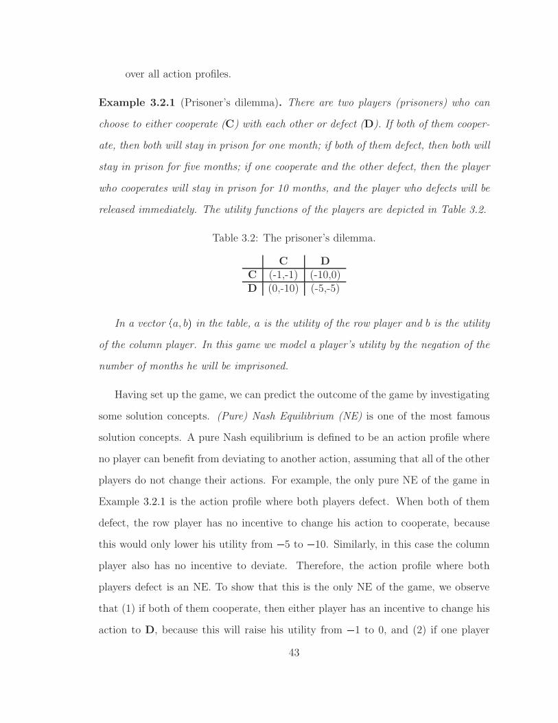
over all action profiles.
Example 3.2.1 (Prisoner’s dilemma). There are two players (prisoners) who can
choose to either cooperate (C) with each other or defect (D). If both of them cooper-
ate, then both will stay in prison for one month; if both of them defect, then both will
stay in prison for five months; if one cooperate and the other defect, then the player
who cooperates will stay in prison for 10 months, and the player who defects will be
released immediately. The utility functions of the players are depicted in Table 3.2.
Table 3.2: The prisoner’s dilemma.
C DC (-1,-1) (-10,0)D (0,-10) (-5,-5)
In a vector pa, bq in the table, a is the utility of the row player and b is the utility
of the column player. In this game we model a player’s utility by the negation of the
number of months he will be imprisoned.
Having set up the game, we can predict the outcome of the game by investigating
some solution concepts. (Pure) Nash Equilibrium (NE) is one of the most famous
solution concepts. A pure Nash equilibrium is defined to be an action profile where
no player can benefit from deviating to another action, assuming that all of the other
players do not change their actions. For example, the only pure NE of the game in
Example 3.2.1 is the action profile where both players defect. When both of them
defect, the row player has no incentive to change his action to cooperate, because
this would only lower his utility from 5 to 10. Similarly, in this case the column
player also has no incentive to deviate. Therefore, the action profile where both
players defect is an NE. To show that this is the only NE of the game, we observe
that (1) if both of them cooperate, then either player has an incentive to change his
action to D, because this will raise his utility from 1 to 0, and (2) if one player
43

cooperates and the other player defects, then the former has an incentive to change
his action to D, because this will raise his utility from 10 to 5. Hence, there is
no other NE except the action profile where both players defect.
In a game, if for a player the following two conditions hold: (1) choosing an action
a never gives her a lower utility than choosing another action b, no matter what the
other players’ action are, and (2) sometimes choosing a gives her a strictly higher
utility than choosing b, then we say that a (weakly) dominates b for that player. Here
b is said to be (weakly) dominated. If choosing a always gives the player a strictly
higher utility than choosing b, then we say that a strictly dominates b. For example,
in the prisoner’s dilemma (Example 3.2.1), C is strictly dominated by D. A strictly
dominated action will never be played in an NE.
In a voting setting we use linear orders over alternatives to model voters prefer-
ences, instead of utility functions. Hence, the simultaneous-move voting games are
defined as follows.
Definition 3.2.2. A simultaneous-move voting game consists of the following com-
ponents.
• There is a set of m alternatives C and a set of n voters (players).
• For each voter, the set of actions is LpCq, which is the set of all linear orders
over C.
• There is a voting rule r that selects a unique winner for each profile.
• For each voter, there is a linear order over C that represents her true prefer-
ences.
The concept of pure NE naturally carries over to simultaneous-move voting games.
In such games, a pure NE is a profile where no single voter can improve the winner
44

by casting a different vote, assuming that the other voters do not change their votes.
Unlike in the prisoner’s dilemma, where there is only one NE, for almost all common
voting rules there are many trivial NE. In fact, for all common voting rules, if the
number of voters is large enough, then there are many profiles where no single voter
can even change the winner by voting differently. For example, suppose there are
three voters whose true preferences are Obama¡Clinton¡McCain, and the plurality
rule with lexicographic tie-breaking is used to select the winner. In the profile where
all three voters vote for McCain¡Clinton¡Obama, no single voter can change the
winner by voting differently. Therefore, this profile is an NE, in which the winner is
the least preferred alternative in all voters’ true preferences. It is easy to see that,
generally, any alternative is the winner in some NE of simultaneous-move voting
games. This observation suggests that pure Nash equilibrium, as a solution concept,
is too coarse for analyzing voting games. One refinement was proposed by Farquhar-
son (1969), who proposed to focus on Nash equilibria in a reduced voting game, where
all iteratively dominated votes are eliminated. However, after iteratively removing
all dominated votes, in general there still too many Nash equilibria.
A solution concept that will play an important role in this dissertation is subgame-
perfect Nash Equilibrium (SPNE). SPNE are defined for extensive-form games, which
consist of multiple stages. For simplicity, here we only define extensive-form games
with perfect information.
Definition 3.2.3. An extensive-form game with perfect information is represented
by a tree and the following components.
• Each (decision) vertex of the tree is labeled by a player, who chooses an action
at the vertex. Each action corresponds to an edge going deeper towards the
leaves.
• Each leaf node is associated with an outcome vector that assigns a real value to
45

each player.
Example 3.2.4. Consider the two prisoners in Example 3.2.1. Now suppose that
in the first stage the row player (player 1) chooses to cooperate or defect. Then in
the second stage, the column player (player 2) chooses his action. Furthermore, we
suppose that player 2 can observe player 1’s action (that is, he has perfect information
about player 1’s move). This situation can be modeled by the extensive-form game
depicted in Figure 3.1.
1
2 2
(-1,-1) (-10,0) (0,-10) (-5,-5)
C D
C D C D
Figure 3.1: An extensive-form game.
In extensive-form games, a player must choose an action for each of her decision
vertices. All these actions together constitute a strategy of the player. A strategy pro-
file constitutes a strategy for each player. A (pure) subgame-perfect Nash equilibrium
is not only a Nash equilibrium, but is also a Nash equilibrium of the extensive-form
game represented by any sub-tree of the original extensive-form game. For example,
the only SPNE of the game in Example 3.2.4 is the strategy profile where player
1 chooses to defect, and player 2 chooses to defect at both of his decision vertices.
SPNE can be computed by a technique called backward induction, which starts with
the bottom decision vertices, and computes the optimal actions for the players at
these decision vertices. Then, we move up to the layer above it. Since we can predict
the outcome at each decision vertex in the lower layer, we can then compute the
optimal actions for the players at the decision vertices in the current layer. And
46

after this, we move up to the next layer above, etc., until the optimal action for the
root vertex has been computed.
It is straightforward to define an extensive-form game for voting. In Chapter 7,
we will study an extensive-form voting game where voters vote one after another.
We call such games Stackelberg voting games. One nice property about Stackelberg
voting games is that, for each Stackelberg voting game, the winner is the same in all
SPNE. This allows us to focus on analyzing the quality of the winner, rather than
analyzing which NE should be the outcome (this problem is known as the equilibrium
selection problem). In Chapter 11, we will see another extensive-form game defined
specifically for combinatorial voting, where the voters vote simultaneously, but they
vote over one issue after another. We call such games strategic sequential voting
processes (SSP). For SSP we will focus on a solution concept that is similar to
SPNE. Under this solution concept, the winner in any such SSP is unique, and can
be computed by a technique that is similar to backward induction.
3.3 Summary
In this chapter, we reviewed some literature on game-theoretic aspects of voting. In
Section 3.1, I gave a brief overview of previous work on using computational com-
plexity as a barrier against manipulation. In Section 3.2, we recalled basic definitions
of normal-form and extensive-form games, and solution concepts such as (pure) Nash
equilibrium and (pure) subgame-perfect Nash equilibrium. We also pointed out that
the biggest challenge in analyzing simultaneous-move voting games is the equilibrium
selection problem, which, as we will see, is alleviated in extensive-form voting games.
47

4
Computational Complexity of Unweighted
Coalitional Manipulation
In this chapter, we will study the computational complexity of manipuation for three
common voting rules. We will prove that the unweighted coalitional manipulation
problem (Definition 3.1.2) is NP-complete for maximin (Section 4.1) and ranked pairs
(Section 4.2), and we will give a polynomial-time algorithm for UCM for Bucklin
(Section 4.3).
4.1 Manipulation for Maximin is NP-complete
In this section, we prove that the UCM problem for maximin is NP-complete. The
proof uses a reduction from the two vertex disjoint paths in directed an-
tisymmetric graph problem, which is known to be NP-complete (Fortune et al.,
1980).
Definition 4.1.1. The two vertex disjoint paths in directed graph problem
is defined as follows. We are given a directed graph G and two disjoint pairs of
vertices pu, u1q and pv, v1q, where u, u1, v, v1 are all different from each other. We
48

are asked whether there exist two directed paths u Ñ u1 Ñ . . . Ñ uk1Ñ u1 and
v Ñ v1 Ñ . . . Ñ vk2Ñ v1 such that u, u1, u1, . . . , uk1
, v, v1, v1, . . . , vk2are all different
from each other.
Theorem 4.1.2. The UCM problem for maximin is NP-complete, for any fixed
number of manipulators n1 ¥ 2.
Proof. It is easy to verify that the UCM problem for maximin is in NP. We now show
that UCM is NP-hard, by giving a reduction from two vertex disjoint paths
in directed graph.
Let the instance of two vertex disjoint paths in directed graph be
denoted by G pV, Eq, pu, u1q and pv, v1q where V tu, u1, v, v1, c1, . . . , cm5u.Without loss of generality, we assume that every vertex is reachable from u or v
(otherwise, we can remove the vertex from the instance). We also assume thatpu, v1q R E and pv, u1q R E (since such edges cannot be used in a solution). Let
G1 pV, E Y tpv1, uq, pu1, vquq, that is, G1 is the graph obtained from G by addingpv1, uq and pu1, vq.We construct a UCM instance as follows.
Set of alternatives: C tc, u, u1, v, v1, c1, . . . , cm5u.Alternative preferred by the manipulators: c.
Number of unweighted manipulators: any fixed number n1 ¥ 2.
Non-manipulators’ profile: P NM satisfying the following conditions:
1. For any c1 c, DP NM pc, c1q 4n1.2. DP NM pu, v1q DP NM pv, u1q 4n1.3. For any ps, tq P E such that DP NM pt, sq is not defined above, we let DP NM pt, sq 2n1 2.
49
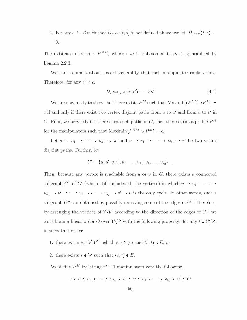
4. For any s, t P C such that DP NM pt, sq is not defined above, we let |DP NM pt, sq| 0.
The existence of such a P NM , whose size is polynomial in m, is guaranteed by
Lemma 2.2.3.
We can assume without loss of generality that each manipulator ranks c first.
Therefore, for any c1 c,
DP NMYP M pc, c1q 3n1 (4.1)
We are now ready to show that there exists P M such that MaximinpP NMYP Mq c if and only if there exist two vertex disjoint paths from u to u1 and from v to v1 in
G. First, we prove that if there exist such paths in G, then there exists a profile P M
for the manipulators such that MaximinpP NM Y P Mq c.
Let u Ñ u1 Ñ Ñ uk1Ñ u1 and v Ñ v1 Ñ Ñ vk2
Ñ v1 be two vertex
disjoint paths. Further, let
V 1 tu, u1, v, v1, u1, . . . , uk1, v1, . . . , vk2
u .
Then, because any vertex is reachable from u or v in G, there exists a connected
subgraph G of G1 (which still includes all the vertices) in which u Ñ u1 Ñ Ñuk1
Ñ u1 Ñ v Ñ v1 Ñ Ñ vk2Ñ v1 Ñ u is the only cycle. In other words, such a
subgraph G can obtained by possibly removing some of the edges of G1. Therefore,
by arranging the vertices of VzV 1 according to the direction of the edges of G, we
can obtain a linear order O over VzV 1 with the following property: for any t P VzV 1,it holds that either
1. there exists s P VzV 1 such that s ¡O t and ps, tq P E, or
2. there exists s P V 1 such that ps, tq P E.
We define P M by letting n1 1 manipulators vote the following.
c ¡ u ¡ u1 ¡ ¡ uk1¡ u1 ¡ v ¡ v1 ¡ . . . ¡ vk2
¡ v1 ¡ O
50

We also let the remaining manipulator vote the following.
c ¡ v ¡ v1 ¡ ¡ vk2¡ v1 ¡ u ¡ u1 ¡ . . . ¡ uk1
¡ u1 ¡ O
Then, we have the following calculations:
DP NMYP M pu, v1q 4n1 pn1 1q 1 3n1 2 3n1 ,
and DP NMYP M pv, u1q 4n1 1 pn1 1q 5n1 2 3n1 .
Moreover, for any t P Cztc, u, vu, there exists s P Cztcu such that ps, tq P E and
DP M pt, sq n1, which means that
DP NMYP M pt, sq 2n1 2 n1 3n1 2 3n1It now follows from Equation (4.1) thatMaximinpP NM Y P Mq c.
Next, we prove that if there exists a profile P M for the manipulators such that
MaximinpP NM Y P Mq c, then there exist two vertex disjoint paths from u to u1and from v to v1.
We define a function f : V Ñ V such that DP NMYP M pt, fptqq 3n1. Indeed,
such a function exists since MaximinpP NM Y P Mq c. Hence, for any t c there
must exist s such that
DP NMYP M pt, sq 3n1Moreover, s must be a parent of t in G1. If there exists more than one such s, define
fptq to be any one of them.
It follows that if pt, fptqq is neither pu, v1q or pv, u1q, then pfptq, tq P E and
DP M pt, fptqq n1, which means that fptq ¡ t in each vote of P M ; otherwise,
if pt, fptqq is pu, v1q or pv, u1q, then DP M pt, fptqq ¤ n1 2, which means that fptq ¡ t
in at least one vote of P M .
51

Now, since |V| m 1 is finite, there must exist l1 l2 ¤ m such that f l1puq f l2puq. That is,
f l1puq Ñ f l11puq Ñ Ñ f l21puq Ñ f l2puqis a cycle in G1. We assume that for any l1 ¤ l11 l12 l2, f l1
1puq f l12puq. Now we
claim that pv1, uq and pu1, vq must be both in the cycle, because
1. if neither of them is in the cycle, then in each vote of P M , we must have
f l2puq ¡ f l21puq ¡ f l1puq f l2puq ,
which contradicts the assumption that each vote is a linear order;
2. if exactly one of them is in the cycle—without loss of generality, f l1puq v, f l11puq u1—then in at least one of the votes of P M , we must have
f l2puq ¡ f l21puq ¡ . . . ¡ f l1puq f l2puq ,
which contradicts the assumption that each vote is a linear order.
Without loss of generality, let us assume that f l1puq u, f l11puq v1, f l3puq v, f l31puq u1, where l3 ¤ l2 2. We immediately obtain two vertex disjoint paths:
u f l1puq f l2puq Ñ f l21puq Ñ . . .Ñ f l31puq u1 ,
and v f l3puq Ñ f l31puq Ñ . . . Ñ f l11puq v1. Therefore, UCM for maximin is
NP-complete.
Notice that the NP-completeness of UCM implies the NP-hardness of UCO for
maximin.
52

4.2 Manipulation for Ranked Pairs is NP-complete
In this section, we prove that UCM for ranked pairs is NP-complete (even for a single
manipulator) by giving a reduction from 3SAT.
Definition 4.2.1. The 3SAT problem is defined as follows: Given a set of variables
X tx1, . . . , xqu and a formula Q Q1 ^ . . .^Qt such that
1. for all 1 ¤ i ¤ t, Qi li,1 _ li,2 _ li,3, and
2. for all 1 ¤ i ¤ t and 1 ¤ j ¤ 3, li,j is either a variable x P X, or the negation
of a variable (i.e., x where x P X),
we are asked whether the variables can be set to true or false so that Q is true.
Theorem 4.2.2. The UCM problem for ranked pairs is NP-complete, even when
there is only one manipulator.
Proof. It is easy to verify that UCM for ranked pairs are in NP. We first prove that
UCM is NP-complete. Given an instance of 3SAT, we construct a UCM instance
as follows. Without loss of generality, we assume that for any variable x, x and x
appears in at least one clause, and none of the clauses contain both x and x.
Set of alternatives: C tc, Q1, . . . , Qt, Q11, . . . , Q
1tutx1, . . . , xq, x1, . . . , xqutQl1,1
, Ql1,2, Ql1,3
, . . . , Qlt,1 , Qlt,2, Qlt,3utQ l1,1, Q l1,2
, Q l1,3, . . . , Q lt,1, Q lt,2, Q lt,3u.
Alternative preferred by the manipulator: c.
Number of unweighted manipulators: n1 1.
Tie-breaking mechanism: We recall that in ranked pairs, we first use the parallel-
universe tie-breaking to select multiple winners, then use a fixed-order tie-breaking
mechanism the select the unique winner. In the fixed-order tie-breaking, c is ranked
in the bottom position.
Non-manipulators’ profile: P NM satisfying the following conditions.
53

1. For any i ¤ t, DP NM pc, Qiq 30,DP NM pQ1i, cq 20; for any x P CztQi, Q1i : 1 ¤
i ¤ tu, DP NM pc, xq 10.
2. For any j ¤ q, DP NM pxj , xjq 20.
3. For any i ¤ t, j ¤ 3,
– if li,j xk for some k ¤ q, then DP NM pQi, Qixkq 30, DP NM pQi
xk, xkq
30, DP NM p xk, Qi xkq 30, DP NM pQi xk
, Q1iq 30;
– if li,j xk for some k ¤ q, then DP NM pQi, Qi xkq 30, DP NM pQi
xk, xkq
30, DP NM p xk, Qi xkq 30, DP NM pQi
xk, Q1iq 30, DP NM pQi xk
, Qixkq
20.
4. For any x, y P C, if DP NM px, yq is not defined in the above steps, then DP NM px, yq 0.
For example, when Q1 x1 _ x2 _ x3, DP NM is illustrated in Figure 4.1.
x1
¬x1
Q1
x1
Q1
¬x1
x2
¬x2
Q1
x2
Q1
¬x2
x3
¬x3
Q1
x3
Q1
¬x3
c
Q1
Q′
1
Figure 4.1: DP NM for Q1 x1 _ x2 _ x3.
In Figure 4.1, for any vertices v1, v2, if there is a solid edge from v1 to v2, then
DP NM pv1, v2q 30; if there is a dashed edge from v1 to v2, then DP NM pv1, v2q 20;
54

if there is no edge between v1 and v2 and v1 c, v2 c, then DP NM pv1, v2q 0; for
any x such that there is no edge between c and x, DP NM pc, xq 10.
The existence of such a P NM is guaranteed by Lemma 2.2.3, and the size of P NM
is in polynomial in t and q.
First, we prove that if there exists an assignment v of truth values to X so that
Q is satisfied, then there exists a vote RM for the manipulator such that RPpP NM YtRMuq c. We construct RM as follows.
• Let c be on the top of RM .
• For any k ¤ q, if vpxkq J (that is, xk is true), then xk ¡RM xk, and for any
i ¤ t, j ¤ 3 such that li,j xk, let Qixk¡RM
Qi xk.
• For any k ¤ q, if vpxkq K (that is, xk is false), then xk ¡RMxk, and for
any i ¤ t, j ¤ 3 such that li,j xk, let Qi xk¡RM
Qixk
.
• The remaining pairs of alternatives are ranked arbitrarily.
If xk J, then DP NMYtRM upxk, xkq 21, and for any i ¤ t, j ¤ 3 such that
li,j xk, DP NMYtRM upQi xk, Qi
xkq 19. It follows that no matter how ties are
broken when applying ranked pairs to P NM Y tRMu, if xk J, then xk ¡ xk in
the final ranking. This is because for any li,j xk, DP NMYtRM upQi xk, Qi
xkq 19
21 DP NMYtRM upxk, xkq, which means that before trying to fix xk ¡ xk, there is
no directed path from xk to xk.
Similarly if xk K, then DP NMYtRM upxk, xkq 19, and for any i ¤ t, j ¤ 3
such that li,j xk, DP NMYtRMupQi xk, Qi
xkq 21. It follows that if xk K, then xk ¡ xk, and for any i ¤ t, j ¤ 3 such that li,j xk, Qi xk
¡ Qixk
in the final
ranking. This is because Qi xk¡ Qi
xkwill be fixed before xk ¡ xk.
Because Q is satisfied under v, for each clause Qi, at least one of its three literals
is true under v. Without loss of generality, we assume vpli,1q J. If li,1 xk, then
55

before trying to add Q1i ¡ c, the directed path c Ñ Qi Ñ QxkÑ xk Ñ xk Ñ
Q xkÑ Q1i has already been fixed. Therefore, c ¡ Q1i in the final ranking, which
means that for any alternatives x in Cztc, Q1, . . . , Qt, Q11, . . . , Q
1tu, c ¡ x in the final
ranking because DP NMYtRM upc, xq ¡ 0. Hence, c is the unique winner of P NMYtRMuunder ranked pairs.
Next, we prove that if there exists a vote RM for the manipulator such that
RPpP NM Y tRMuq c, then there exists an assignment v of truth values to X
such that Q is satisfied. We construct the assignment v so that vpxkq J if and
only if xk ¡RM xk, and vpxkq K if and only if xk ¡RM
xk. We claim that
vpQq J. If, on the contrary, vpQq K, then there exists a clause (Q1, without
loss of generality) such that vpQ1q K. We now construct a way to fix the pairwise
rankings such that c is not the winner for ranked pairs, as follows. For any j ¤ 3,
if there exists k ¤ q such that li,j xk, then xk ¡RM xk because vp xkq K.
Therefore, DP NMYRMpxk, xkq 21. Then, after trying to add all pairs x ¡ x1
such that DP NMYRMpx, x1q ¡ 21 (that is, all solid directed edges in Figure 4.1),
it follows that xk ¡ xk can be added to the final ranking. We choose to add
xk ¡ xk first, which means that Q1xk
¡ Q1 xkin the final ranking (otherwise, we
have Q1 xk¡ Q1
xk¡ xk ¡ xk ¡ Q1 xk
, which is a contradiction).
For any j ¤ 3, if there exists k ¤ q such that li,j xk, then xk ¡RMxk because
vpxkq K. Therefore, DP NMYRMpxk, xkq 19. We note that after trying to add
all pairs x ¡ x1 such that DP NMYRMpx, x1q ¡ 19, Q1
xk£ Q1 xk
. We recall that for
any j ¤ 3, if there exists k ¤ q such that li,j xk, then Q1 xk£ Q1
xk. Hence,
it follows that Q11 ¡ c is consistent with all pairwise rankings added so far. Then,
since DP NMYRMpQ11, cq ¥ 19, if Q11 ¡ c has not been added, we choose to add it
first of all pairwise rankings of alternatives x ¡ x1 such that DP NMYRMpx, x1q 19,
which means that Q11 ¡ c in the final ranking—in other words, c is not at the top
in the final ranking. Therefore, c is not the unique winner, which contradicts the
56
assumption that RPpP NM Y tRMuq c.
Similarly, we can prove that when k is a constant greater than one, UCM for
ranked pairs remain NP-complete.
Theorem 4.2.3. The UCM problem for ranked pairs is NP-complete, for any fixed
number of manipulators n1 ¥ 2.
Proof. The proof is similar to that of Theorem 4.2.2. We let P NM satisfy the follow-
ing conditions.
1. For any i ¤ t, DP NM pc, Qiq 30n1,DP NM pQ1i, cq 22n1 2; for any x PCztQi, Q
1i : 1 ¤ i ¤ tu, DP NM pc, xq 10n1.
2. For any j ¤ q, DP NM pxj , xjq 22n1 2.
3. For any i ¤ t, j ¤ 3, if li,j x, then DP NM pQi, Qixq 30n1, DP NM pQi
x, xq 30n1, DP NM p x, Qi xq 30n1, DP NM pQi x, Q
1iq 30n1; if li,j x, then
DP NM pQi, Qi xq 30n1, DP NM pQi
x, xq 30n1, DP NM p x, Qi xq 30n1,DP NM pQi
x, Q1iq 30n1, DP NM pQi x, Q
ixq 20n1.
4. For any y, y1 P C, if DP NM py, y1q is not defined in the above steps, then
DP NM py, y1q 0.
First, if there exists an assignment v of truth values to X so that Q is satisfied, then
we let RM be defined as in the proof for Theorem 4.2.2. It follows that RPpP NM Ytn1RMuq c (all the manipulators can vote RM).
Next, if there exists a profile P M for the manipulators such that RPpP NMYP Mq c, then we construct the assignment v so that vpxq J if x ¡V x for all V P P M ,
and vpxq K if x ¡V x for all V P P M ; the values of all the other variables are
assigned arbitrarily. Then by similar reasoning as in the proof for Theorem 4.2.2, we
know that Q is satisfied under v.
57
4.3 A Polynomial-time Algorithm for Manipulation for Bucklin
In this section, we present a polynomial-time algorithm for the UCM problem for
Bucklin.
For any alternative x P C, any natural number d P N, and any profile P , let
Bpx, d, P q denote the number of times that x is ranked among the top d alternatives
in P . The idea behind the algorithm is as follows. Let dmin denote the Bucklin score
of x in P , that is, dmin is the minimal depth so that the favorite alternative c is
ranked among the top dmin alternatives in more than half of the votes (when all of
the manipulators rank c first). Then, we simply check if there is a way to assign
the manipulators’ votes so that none of the other alternatives is ranked among the
top dmin alternatives in more than half of the votes. In other words, the order of
the alternatives is not crucial, only their membership in the set of dmin top-ranked
alternatives is relevant.
Algorithm 1.
Input. A UCM instance pBucklin, P NM , c, n1q, where C tc, c1, . . . , cm1u.1Stage 0.
0.1 Calculate the Bucklin score dmin such that
Bpc, dmin, PNMq n1 ¡ 1
2p|P NM | n1q
0.2 If there exists c1 P C, c1 c such that
Bpc1, dmin, PNMq ¡ 1
2p|P NM | n1q , (4.2)
then output that there is no successful manipulation.
1 This algorithm works for the fixed-order tie-breaking mechanism where c is ranked in the bottomposition. Similar algorithms can be designed for other fixed-order tie-breaking mechanisms.
58

Aside. Notice that dmin is defined under the assumption that all the manipulators
rank c first. Consider an alternative c1 c that satisfies the condition in Equa-
tion (4.2). Such an alternative is ranked in the top dmin positions of half the votes
P NM Y P M , regardless of P M . Hence, c cannot be a unique winner.
Stage 1.
1.1 For every c1 P Cztcu, let
dc1 Z1
2p|P NM | n1q^Bpc1, dmin, P
NMq ,
and let kc1 mintdc1, n1u.1.2 If
c1c
kc1 pdmin 1qn1 , (4.3)
then output that there is no successful manipulation.
Aside. kc1 is the number of times that we can place c1 in the first dmin positions of
the votes of P M , without compromising the victory of c. In particular, kc1 cannot be
greater than n1.Notice that there are exactly pdmin 1qn1 problematic positions to fill, since c
is ranked first by all the manipulators. Now, if the condition in Equation (4.3) is
satisfied, for any P M there must be an alternative c1 that appears too many times
in the first dmin positions, that is, kc1 Bpc1, dmin, PMq. Since Bpc1, dmin, P
Mq ¤ n1,we have in particular that kc1 n1, hence it must hold that kc1 dc1. It follows that
Bpc1, dmin, PNM Y P MqBpc1, dmin, PNMq Bpc1, dmin, P
Mq¡Bpc1, dmin, PNMq dc1 Z1
2p|P NM | n1q
59

Therefore, c cannot be a unique winner.
Stage 2. Construct P M by assigning the alternatives to the first dmin positions of
the votes in a way that for every t 1, . . . , m 1,
Bpct, dmin, PMq ¤ kct (4.4)
Complete the rest of the votes arbitrarily. Return P M as a successful manipulation.
Aside. Given that (4.3) does not hold, it is clearly possible to construct P M such
that (4.4) holds for every c1 c. Moreover, this can be done in polynomial time, e.g.,
by enumerating the alternatives and placing each alternative in the next position in
kc1 of the votes of the manipulators, until the crucial positions are filled.
Now, for every t 1, . . . , m 1 it holds that
Bpct, dmin, PNM Y P Mq ¤ Bpct, dmin, P
NMq kct¤ 1
2p|NM | n1q ,
which implies that BucklinpP NM Y P Mq c.
We have obtained the following result.
Theorem 4.3.1. Algorithm 1 correctly decides the UCM problem in polynomial time.
It is easy to see that the tractability of UCM for Bucklin implies that UCO can
be solved in polynomial time as well.
4.4 Summary
In this chapter, we investigated the computational complexity of the UCM and UCO
problems for the maximin, ranked pairs, and Bucklin rules. The UCM problem is NP-
complete under the maximin rule for any fixed number (at least two) of manipulators.
The UCM problem is also NP-complete under the ranked pairs rule; in this case, the
60

hardness holds even if there is only a single manipulator, similarly to second-order
Copeland (Bartholdi et al., 1989a) and STV (Bartholdi and Orlin, 1991). Finally,
we gave a polynomial-time algorithm for the UCM problem under the Bucklin rule.
It should be noted that all of our NP-hardness results, as well as the ones men-
tioned in the introduction, are worst-case results. Hence, there may still be an
efficient algorithm that can find a beneficial manipulation for most instances. In-
deed, nearly a dozen recent papers suggest that finding manipulations is easy with
respect to some typical distributions on preference profiles. We will see some of them
in the next chapter.
61
5
Computing Manipulations is “Usually” Easy
We have seen in the last chapter that computing a manipulation is NP-complete
for maximin and ranked pairs. In particular, the coalitional manipulation problem
is NP-complete for ranked pairs even for one manipulator. This property was only
shown previously for STV and second-order Copeland. In Table 3.1 we observe that
computational complexity can serve as a barrier for many common voting rules when
there are two or more manipulators. In this chapter, we will prove that computa-
tional complexity is not a strong barrier against manipulation for almost all common
voting rules. This argument will be supported by two approaches. In Section 5.2 we
pursue the “frequency of manipulability” approach, that is, the votes are randomly
generated i.i.d. according to some distribution over all linear orders. We will show
that with a high probability the UCM problem (Definition 3.1.2) is computationally
trivial. In Section 5.4 we pursue an approximation approach. More precisely, we fo-
cus on approximating the UCO problem (Definition 3.1.3), and propose an algorithm
that approximates UCO with an additive error that only depends on the number of
alternatives (but not on the number of voters) for all positional scoring rules.
Instead of proving the results one by one for common voting rules, we take unified
62
approaches. In Section 5.1 we introduce a general framework called generalized scor-
ing rules, and then characterize the frequency of manipulability for any generalized
scoring rule in Section 5.2. To show how general this class of voting rules is, we
give a concise axiomatic axiomatization in Section 5.3. In Section 5.4 we will design
an approximation algorithm that works for any positional scoring rule, in light of a
novel relationship between UCO and a scheduling problem.
5.1 Generalized Scoring Rules
A generalized scoring rule (GSR) associates a vector of k real numbers with every
vote, for some k that depends on (but is not necessarily equal to) m. The decision
that the rule makes is based only on the sum of these vectors. Even more specifically,
the decision is based only on comparisons among the components in this sum. That
is, if we know, for every i, j P t1, . . . , ku, whether the ith component in the sum is
larger than the jth component, the jth is larger than the ith, or they are the same,
then we know enough to determine the winner. Sometimes, the components can be
partitioned so that the decision only depends on comparisons within elements of the
partition, which will be helpful.
Let k P N, and let K tK1, . . . , Kqu be a partition of K t1, . . . , ku. That is,
for any i ¤ q, Ki K, K q
l1 Kl, and for any i, j ¤ q, i j, Ki XKj H. We
say that two vectors of length k are equivalent with respect to a partition if, within
each element of the partition, they agree on which components are larger.
Definition 5.1.1. Let K be a partition of K. For any a, b P Rk, we say that a and b
are equivalent with respect to K , denoted by a K b, if for any l ¤ q, any i, j P Kl,
ai ¥ aj bi ¥ bj (where ai denotes the ith component of the vector a, etc.).
For two partitions K tK1, . . . , Kqu and K 1 tK 11, . . . , K
1pu, K 1 is a refine-
ment of K if for any l ¤ q, any l1 ¤ p, K 1l1 X Kl is either K 1
l1 or H. That is, K 163

is obtained from K by partitioning the sets in K . In this case, we say that K is
coarser than K 1, and K 1 is finer than K .
Proposition 5.1.2. For any partitions K , K 1 such that K 1 is a refinement of K ,
and any a, b P Rk, if a K b, then a K 1 b.
We note that tKu (the partition that only contains K itself) is the coarsest
partition.
Definition 5.1.3. Let K be a partition of K. A function g : Rk Ñ C is compatible
with K if for any a, b P Rk, a K b ñ gpaq gpbq.That is, for any mapping g that is compatible with K , gpaq is determined (only)
by comparisons within each Kl, l ¤ q. Namely, we do not need to compare compo-
nents across different elements of the partition.
Now we are ready to define generalized scoring rules.
Definition 5.1.4. Let k P N, f : LpCq Ñ Rk and g : Rk Ñ C, where g is compatible
with K . f and g determine the generalized scoring rule GSpf, gq as follows. For
any profile of votes V1, . . . , Vn P LpCq, GSpf, gqpV1, . . . , Vnq gp°n
i1 fpViqq. We say
that GSpf, gq is of order k, and compatible with K .
From Proposition 5.1.2 we know that for any partitions K , K 1 such that K 1 is
a refinement of K , GSpf, gq is compatible with K 1, then GSpf, gq is also compat-
ible with K . Given a profile P of votes, we use fpP q as shorthand for°
V PP fpV q.We will call fpP q the total generalized score vector. By definition, any unweighted
generalized scoring rule satisfies anonymity (that is, every voter is treated equally)
and homogeneity (that is, if we add any number of copies of the profile to the pro-
file, the winner does not change). Any generalized scoring rule is compatible with
the partition tKu. Nevertheless, being compatible with tKu is not vacuous: if we
64
modified the definition so that g is not required to be compatible with any partition,
then any anonymous voting rule would belong to the resulting class of rules. If a
generalized scoring rule is compatible with a partition, this effectively means that,
within each element of the partition, the scores are of the same “type,” so that we
can compare them.
We now illustrate how general the class of generalized voting rules is by showing
how some standard rules belong to the class. Many other rules can also be shown to
belong to the class.
Proposition 5.1.5. All positional scoring rules, Copeland, STV, maximin, ranked
pairs, and Bucklin are generalized scoring rules.
Proof of Proposition 5.1.5: We explicitly give k, f, g, K for each of these rules.
In the remainder of the proof, the number of alternatives is fixed to be m. Let
V P LpCq be a vote, and let P be a profile of votes. To simplify the construction,
we will not specify how ties are broken when we describe these rules as generalized
scoring rules. It is easy to incorporate the tie-breaking mechanism to define the g
function for all these voting rules.
Positional scoring rules: Suppose the scoring vector for the rule is
~sm psmp1q, . . . , smpmqq. The total generalized score vector will simply consist of
the total scores of the individual alternatives. Let
• k~sm m.
• f~smpV q p~smpV, c1q, . . . , ~smpV, cmqq.• g~smpf~vpP qq arg maxipf~vpP qqi.• K~sm tKu.
Copeland: For Copeland, the total generalized score vector will consist of the scores
in the pairwise elections. Let
65

• kCopeland mpm 1q; the components are indexed by pairs pi, jq such that
i, j ¤ m, i j.
• pfCopelandpV qqpi,jq " 1 if ci ¡V cj
0 otherwise
• gCopeland selects the winner based on fCopelandpP q as follows. For each pair i j,
if pfCopelandpP qqpi,jq ¡ pfCopelandpP qqpj,iq, then add 1 point to i’s Copeland score;
if pfCopelandpP qqpj,iq ¡ pfCopelandpP qqpi,jq, then add 1 point to j’s Copeland score;
if tied, then add 0.5 to both i’s and j’s Copeland scores. The winner is the
alternative that gets the highest Copeland score.
• qCopeland mpm1q2
(we recall that q is the number of elements in the partition).
The elements of the partition are indexed by pi, jq, i j. For any l pi, jq,i j, let Kl tpi, jq, pj, iqu. Let KCopeland tKl : l pi, jq, i ju.
STV: For STV, we will use a total generalized score vector with many components.
For every proper subset S of alternatives, for every alternative c outside of S, there
is a component in the vector that contains the number of times that c is ranked first
if all of the alternatives in S are removed. Let
• kSTV °m1i0
m
i
pm iq; the components are indexed by pS, jq, where S is a
proper subset of C and j ¤ m, cj R S.
• pfSTV pV qqpS,jq 1, if after removing S from V , cj is at the top; otherwise, letpfSTV pV qqpS,jq 0.
• gSTV selects the winner based on fSTV pP q as follows. In the first round,
find j1 arg minjppfSTV pP qqpH,jqq. Let S1 tcj1u. Then, for any 2 ¤i ¤ m 1, define Si recursively as follows: Si Si1 Y tjiu, where ji arg minjpfSTV pP qpSi1,jqq; finally, the winner is the unique alternative in C Sm1.
66

• qSTV 2m 1. The elements of the partition are indexed by the S C. For
any S C, let KS tpS, jq : cj R Su. Let KSTV tKS : S Cu.Maximin: For maximin, we use the same total generalized score vector as for
Copeland, that is, the vector of all scores in pairwise elections. Let
• kmaximin mpm 1q; the components are indexed by pairs pi, jq such that
i, j ¤ m, i j.
• pfmaximinpV qqpi,jq " 1 if ci ¡V cj
0 otherwise
• gmaximinpfmaximinpP qq is the ci such that for any i1 ¤ m, i1 i, there exists
j1 m, j1 i1 such that for any j ¤ m, j i, we have fmaximinpP qpi,jq ¡pfmaximinpP qqpi1,j1q.• Kmaximin tKu.
Ranked pairs: We use the same total generalized score vector as for Copeland and
maximin, that is, the vector of all scores in pairwise elections. Let
• krp mpm 1q; the components are indexed by pairs pi, jq such that i, j ¤ m,
i j.
• pfrppV qqpi,jq " 1 if ci ¡V cj
0 otherwise
• grp selects the winner based on frppP q as follows. In each step, we consider a
pair of alternatives ci, cj that we have not previously considered; specifically, we
choose the remaining pair with the highest pfrppP qqpi,jq. We then fix the order
ci ¡ cj , unless this contradicts previous orders that we fixed (that is, it violates
transitivity). We continue until we have considered all pairs of alternatives.
The alternative at the top of the ranking wins.
67
• Krp tKu.Bucklin: For Bucklin, the total generalized score vector will have one component
for every combination of an alternative and a position; this component contains the
number of times that that alternative is ranked either in that position or in a higher
position. We only need to consider positions from 1 through m 1. Let
• kBucklin 2mpm 1q; the components are indexed by pi, jq1 and pi, jq2, i ¤m 1, j ¤ m.
• fBucklinpV qpi,jq1 1 and fBucklinpV qpi,jq2 0 if cj is ranked among the top i
alternatives in V ; otherwise fBucklinpV qpi,jq1 0 and fBucklinpV qpi,jq2 1.
• gBucklinpfBucklinpP qq is the cj such that there exists i ¤ m, pi, jq1 ¡ pi, jq2, and
for any j1 j, pi, j1q2 ¥ pi, jq1.• qBucklin m 1. For any l ¤ m 1, let Kl tpl, jq1, pl, jq2 : j ¤ mu. Let
KBucklin tKl : l ¤ mu. lWe have shown that STV is a generalized scoring rule in the proof. In fact, we can
generalize this and show that any multiround run-off process where in each round,
alternatives are eliminated according to a generalized scoring rule (to be precise, a
correspondence) must itself be a generalized scoring rule. For example, for STV,
the voting rule that only eliminates one alternative (the alternative that has the
lowest plurality score among all remaining alternatives) is used in every round. As
another example, for Baldwin’s rule, a reverse version of Borda that only eliminates
one alternative (the alternative that has the lowest Borda score among all remaining
alternatives) is used in every round. The proof can be found in the appendix of Xia
and Conitzer (2008b), and is omitted here.
68

5.2 Frequency of Manipulability for Generalized Scoring Rules
Let π be a probability distribution over LpCq that is positive everywhere. For any
n P N, let φπ,n be the distribution over profiles of n voters in which each vote is
drawn i.i.d. according to π. Given a manipulation instance pr, P NM , c, n1q, if there
is only one possible winner, then we say that this manipulation instance is closed;
otherwise we say this manipulation instance is open (Procaccia and Rosenschein,
2007a).
Definition 5.2.1. A manipulation instance pr, P NM , c, n1q is closed if for any profiles
P M1 , P M
2 for the manipulators, rpP NM YP M1 q rpP NM YP M
2 q. An instance is open
if it is not closed.
We note that in the above definition, whether a UCM instance is open or closed
does not depend on the choice of c. That is, for any c, c1 P C, pr, P NM , c, n1q is
open (respectively, closed) if and only if pr, P NM , c1, n1q is open (respectively, closed).
Procaccia and Rosenschein (2007a) have shown that, suppose the following four
conditions are satisfied.
1. The rule is a positional scoring rule,
2. the number of manipulators |M | is op?nq,3. the votes are drawn independently, and
4. there exists d ¡ 0 such that for each vote’s distribution, the variance of the
difference in scores for any pair of alternatives is at least d.
Then, when n Ñ 8, the probability that a weighted manipulation instance is
open is 0. In this section, we generalize this result to generalized scoring rules; in
addition, we characterize the rate of convergence to 0. However, unlike Procaccia and
69

Rosenschein, we do assume that votes are drawn i.i.d.; this is needed to obtain the
convergence rate. Hence, strictly speaking, our result is not a generalization of their
result. We can also obtain a strict generalization of Procaccia and Rosenschein’s
results to generalized scoring rules, but without proving a convergence rate; we will
not do so in this paper.
5.2.1 Conditions under Which Coalitional Manipulability is Rare
In this section, we study the probability that a manipulation instance is open when
there are Opnαq (0 ¤ α 12) manipulators, and the nonmanipulator votes are drawn
i.i.d. Let n |P NM | denote the number of nonmanipulators. Then, n is the total
number of voters, n n1 (nonmanipulators and manipulators). We will prove that
for any generalized scoring rule, this probability is Op 1?nq. Let T pr, m, n, π, n1q denote
this probability. That is, let c be an arbitrary alternative,
T pr, m, n, π, n1q PrP NMφπ,n tpr, P NM , c, n1q is openuLemma 5.2.2. Let N P N. Let Y1, . . . , YN be i.i.d. random variables with EpY1q 8,
EppY1EpY1qq2q ¡ 0, and Ep|Y1EpY1q|3q 8. Let Y °N
ζ1 Yζ. For any constant
0 ¤ p 12
that does not depend on N , and any function fpNq that is Ωp1q, we have
that Prp|Y | ¤ fpNqq is OpfpNq?Nq.
Proof of Lemma 5.2.2: Let Φpxq be the cumulative distribution function of the
standard normal distribution Np0, 1q. Let σ2 EppY1 EpY1qq2q, ρ Ep|Y1 EpY1q|3q. Then we have:
Prp|Y | fpNqqPrpEpY1qNσ?
N fpNq
σ?
N Y EpY1qN
σ?
N EpY1qN
σ?
N fpNq
σ?
Nq
70

Then by the Berry-Esseen theorem (Durrett, 1991),
Prp|Y | fpNqq ΦpEpY1qNσ?
N fpNq
σ?
Nq ΦpEpY1qN
σ?
N fpNq
σ?
Nq Cρ
σ3?
N » EpY1qNσ?
N fpNq
σ?
NEpY1qNσ?
N fpNq
σ?
N
Np0, 1qpxqdx Cρ
σ3?
N 2fpNqσ?
N 1?
2π Cρ
σ3?
N
which is OpfpNq?Nq, because C is a constant that does not depend on N and fpNq
Ωp1q. lTheorem 5.2.3. Let r GSpf, gq be a generalized scoring rule of order k. For any
m P N, any constant 0 ¤ α 12, and any constant h (where both m and h do not
depend on n), there exists a constant tm,α,h ¡ 0 (that does not depend on n) such
that if n1 ¤ hnα, then
T pr, m, n, π, n1q ¤ tm,α,hnα 1
2
Proof of Theorem 5.2.3: We recall that each vote is drawn i.i.d. according to π.
For any pair i1, i2 ¤ k, i1 j2, and any t ¡ 0, let
Rpi1, i2, t, π, n1q Prt|pfpP NMqqi1 pfpP NMqqi2| ¤ tuWe recall that pfpP NMqqi is the ith component of fpP NMq. In other words,
Rpi1, i2, t, π, n1q is the probability of profiles of nonmanipulators’ votes P NM such
that the difference between the i1th component and the i2th component of fpP NMqis no more than t, when each vote is drawn i.i.d. according to π. We also recall
that n |P NM |. Let Yi1,i21 , . . . , Y
i1,i2n be n i.i.d. random variables, where the
distribution for each Yi1,i2ζ is the same as the distribution for pfpV qqi1 pfpV qqi2 ,
71

where V is drawn according to π. That is, for any V P LpCq, with probability πpV q,Y
i1,i21 takes value pfpV qqi1 pfpV qqi2. Let Y i1,i2 °n
ζ1 Yζ.
Let vmax maxi¤k,V PLpCqpfpV qqi. That is, vmax is the maximum component of all score
vectors corresponding to a single vote. We note that vmax is a constant that does not
depend on n. We also note that since n1 is Opnαq and α 12, it must be that n is
Ωpnq, so that n is Opnq, vmaxhnα is Oppnqαq. Therefore, by Lemma 5.2.2 (in which
we let N n), we know that Prp|Y i1,i2| ¤ vmaxhnαq is Opvmaxhnα?n q Oppnqα 1
2 q,so it is Opnα 1
2 q. Hence, there exists a constant ti1,i2 such that
Prp|Y i1,i2| ¤ vmaxhnαq ti1,i2nα 1
2
We let tmax maxi,j¤k,ij ti,j. If a manipulation instance is open, then there exists a
profile P M for the manipulators such that GSpf, gqpP M Y P NMq GSpf, gqpP NMq,which means that fpP M YP NMq fpP NMq. In this case there must exist i, j, i j,
such that Prp|pfpP NMqqi pfpP NMqqj| ¤ vmaxnq ¤ vmaxhnα. Therefore,
T pGSpf, gq, m, n, π, n1q ¤ ¸1¤i j¤m
Rpi, j, vmaxhnα, π, n1qWe note that Rpi, j, vmaxhnα, π, n1q Prp|Y i,j| ¤ vmaxhnαq. Therefore, we have
T pGSpf, gq, m, n, π, n1q ¤ij
Rpi, j, vmaxhnα, π, n1q¤ij
ti,jnα1 ¤ kpk 1q
2tmaxn
α 1
2
Let tm,α,h kpk1q2
tmax. We know that tm,α,h is a constant that does not depend on
n.
(End of the proof for Theorem 5.2.3.) lFrom Proposition 5.1.5 and Theorem 5.2.3, we obtain the following corollary.
72
Corollary 5.2.4. Let r be any positional scoring rule, Copeland, STV, maximin,
ranked pairs, or Bucklin. For any m P N, any constant 0 ¤ α 12, and any constant
h (where m, α, and h do not depend on n), there exists a constant tm,α,h ¡ 0 (that
does not depend on n) such that if n1 ¤ hnα, then
T pr, m, n, π, n1q ¤ tm,α,hnα 1
2
A profile is said to be tied if a single additional voter can change the outcome. By
letting α 0 and h 1 in Theorem 5.2.3, we have that for any generalized scoring
rule and any fixed m, the number of tied profiles is Op 1?nq.
5.2.2 Conditions under which Coalitions of Manipulators are All-Powerful
Let us consider a positional scoring rule and a distribution over nonmanipulator
votes. Furthermore, let us consider each alternative’s expected score; let Cmax be
the set of alternatives with the highest expected score. Procaccia and Rosenschein
(2007a) have shown that, suppose the following conditions hold.
1. The number of manipulators is in both ωp?nq and opnq, and
2. votes are drawn i.i.d.
Then, the probability that the manipulators can make any alternative in Cmax
win converges to 1 as n Ñ 8. Hence, assuming |Cmax| ¡ 1, the probability that the
instance is open converges to 1 (however, if |Cmax| 1, it converges to 0).
In this section, we prove a similar result for generalized scoring rules; in addition,
we characterize the rate of convergence to 0. (In fact, in this case, Procaccia and
Rosenschein also characterize this rate—for positional scoring rules.)
Specifically, in this section, we study the case where the number of manipulators
is Ωpnαq (12 α 1) and opnq, the votes are drawn i.i.d. according to π, and a
generalized scoring rule is used. We provide a sufficient condition under which the
73
manipulators can make any alternative in a particular set of alternatives win with
probability 1OpeΩpn2α1qq. (We need the opnq assumption for a technical reason.
If n1 Θpnq, then obviously the probability that the manipulators are all-powerful
is higher.)
Definition 5.2.5. π is compatible with K w.r.t. f , if, for V π, for any l ¤ q,
any i, j P Kl (i j), EppfpV qqiq EppfpV qqjq.That is, π is compatible with K w.r.t. f if within each element of the partition
K , the expectation of the components of fpV q are the same (where V is drawn
according to π).
Given GSpf, gq, it will be useful to have a profile P such that for some partition
K that GSpf, gq is compatible with, the components of fpP q within each Kl (l ¤ q)
are all different. The next definition makes this precise.
Definition 5.2.6. For any GSpf, gq compatible with K , a profile P is said to be
distinctive w.r.t. GSpf, gq and K if for each l ¤ q and each pair i, j P Kl, i j,pfpP qqi pfpP qqj.The next definition concerns the set of alternatives that can be made to win using
a distinctive profile.
Definition 5.2.7. For any GSpf, gq compatible with K , let WK pf, gq be a subset of
the alternatives defined as follows.
WK pf, gq tGSpf, gqpP q : P is distinctive w.r.t. GSpf, gq and K uFor any profile P M of manipulators and any alternative c, we define T pm, n, π, c, P Mq
PrpGSpf, gqpP MYP NMq cq. That is, given a profile of votes P M of the manipula-
tors, T pm, n, π, c, P Mq is the probability that the winner of the profile P M YP NM is
74
c, when the number of alternatives is m, the number of voters is n, and the nonma-
nipulators’ votes P NM are drawn i.i.d. according to π. Now we are ready to present
the theorem.
Theorem 5.2.8. Let GSpf, gq be a generalized scoring rule that is compatible with
K . Let πK be a distribution over LpCq such that πK is compatible with K w.r.t. f .
For any m ¡ 0, there exist constants tm ¡ 0 and um ¡ 0 (neither of which depend on
n) such that for any constant h ¡ 0 (that does not depend on n) and any alternative
c P WK pf, gq, if the number of manipulators is at least hnα (1
2 α 1) (as well as
opnq), then there exists a coalitional manipulation P M such that
T pm, n, πK , c, P Mq ¡ 1 tmeumn2α1
Theorem 5.2.8 states that when the number of alternatives is held fixed, if the
number of manipulators is large (Ωpnαq for α ¡ 12, as well as opnq) then for any
alternative c P WK pf, gq, there exists a manipulation P M such that when the non-
manipulators’ votes are drawn i.i.d. according to πK , then c is the winner with a
probability of 1OpeΩpn2α1qq.Proof of Theorem 5.2.8: Let n1 ¥ hnα. If WK pf, gq H, then Theorem 5.2.8
vacuously holds. So we assume that WK pf, gq H. For each c P WK pf, gq, we
associate c with a distinctive profile (w.r.t. f and K ), denoted by P c , such that
c GSpf, gqpP c q. We recall that P c is distinctive if and only if for each l ¤ q and
each pair i, j P Kl, i j, pfpP c qqi pfpP c qqj . Let
dmin minl¤q,i,jPKl,ij,cPWK pf,gqp|pfpP c qqi pfpP c qqj|q
That is, dmin is the minimal difference between any two components within the
same element of K of fpP c q, taken over all c P WK pf, gq. Since |WK pf, gq| m
(which does not depend on n), and P c is distinctive, we know that dmin ¡ 0 and
75

does not depend on n. Let pmax maxcPC |P c |. That is, for all c P WK pf, gq, the
number of votes in P c is no more than pmax. We note that pmax does not depend on
n.
For any c P C, define a profile of the manipulator votes P Mc as follows. P M
c
consists of two parts:
1. t n1|P c |uP c , and
2. an arbitrary profile for the remaining n1 t n1|P c |u|P c | votes.
That is, P Mc consists mostly of t n1|P c |u copies of P c ; the remaining votes (at most|P c |) are chosen arbitrarily. We note that |P c | is a constant that does not depend
on n, so that the second part becomes negligible when n Ñ8.
The next claim provides a lower bound on the difference between any two com-
ponents of fpP Mc q.
Claim 5.2.1. There exists a constant dc that does not depend on n such that the
minimum difference between components of fpP Mc q is at least dcn
α.
Proof of Claim 5.2.1: Since the minimal difference between any two components
of P c is at least dmin, the minimal difference between any two components of fpP Mc q
is at least t n1|P c |udmin. We note that the number of arbitrarily assigned votes in P Mc
is no more than |P c |, and the difference between any two components in a vote is no
more than vmax. Therefore the minimal difference between any two components of
fpP Mq is at leastt n1|P c |udmin vmax|P c | ¥ p n1pmax
1qdmin vmaxpmax
76

Note that this number is Ωpnαq because pmax, dmin, and vmax are constants that
do not depend on n, and n1 is Ωpnαq. Therefore, there exists a dc that does not depend
on n such that the minimal difference between any two components of fpP Mc q is at
least dcnα.
(End of the proof for Claim 5.2.1.) lThe next lemma is known as Chernoff’s inequality (Chernoff, 1952).
Lemma 5.2.9 (Chernoff’s inequality). Let N P N. Let Y1, . . . , YN be N i.i.d. random
variables with variance σ2. Let Y °N
ζ1 Yζ. For any 0 ¤ l ¤ 2?
Nσ, Prp|Y EpY q| ¥ l
?Nσq ¤ 2el24.
For any profile P NM for the nonmanipulators, any i1, i2 ¤ k, i1 i2, let
DpP NM , i1, i2q |pfpP NMqqi1 pfpP NMqqi2|. The next claim states that if each
vote of P NM is drawn i.i.d. according to πK , then for any different i1, i2 within the
same element Kl of the partition K , the probability that the difference between the
i1th and the i2th component of fpP NMq is larger than dcnα is OpeΩpn2α1qq.
Claim 5.2.2. For any l ¤ q and any i1, i2 P Kl (i1 i2), there exists a constant
dc,i1,i2 ¡ 0 that does not depend on n such that
PrpDpP NM , i1, i2q ¡ dcnαq ¤ 2edc,i1,i2
n2α1
Proof of Claim 5.2.2: Let Yi1,i21 , . . . , Y
i1,i2n be n i.i.d. random variables such that
the distribution for each Yi1,i2ζ is the same as the distribution for pfpV qqi1pfpV qqi2 ,
where V is drawn according to π. That is, for any V P LpCq, with probabil-
ity πpV q, Yi1,i21 takes value pfpV qqi1 pfpV qqi2 . Let Y i1,i2 °|NM |
ζ1 Yi1,i2ζ . Then,
PrpDpP NM , i1, i2q ¡ dcnαq PrpY i1,i2 ¡ dcn
αq.Since πK is compatible with K , for any l ¤ q, i1, i2 P Kl, we know that
EppfpV qqi1q EppfpV qqi2q, where V is drawn according to π. Therefore, EpY i1,i21 q
77

0. Let σ2i1,i2
be the variance of Yi1,i21 . We note that σi1,i2 does not depend on n. If
σ2i1,i2
0, then for any V P LpCq, pfpV qqi1 pfpV qqi2 (because for any V P LpCq,πK pV q ¡ 0), which means that WK pf, gq H. This contradicts the assumption
that WK pf, gq H. Hence σ2i1,i2
¡ 0. Since n1 opnq, n Ωpnq, and for suffi-
ciently large n we have dcnα
σi1,i2
?n ¤ 2σi1,i2
?n. Therefore, we can use Lemma 5.2.9
(in which we let N n) to bound PrpDpP NM , i1, i2q ¡ dcnαq above as follows.
PrpDpP NM , i1, i2q ¡ dcnαqPrp|Y i1,i2| ¡ dcn
αqPrp|Y i1,i2| ¡ dcnα 1
2
σi1,i2
?n σi1,i2
?nq¤2e
p dcnα1
2
σi1,i2
?n q24 (Lemma 5.2.9)¤2e
d2c
4σ2i1,i2
n2α1 pn ¤ nqWe note that d2
c
4σ2i1,i2
is a constant that does not depend on n. Therefore, there
exists uc,i1,i2 ¡ 0 such that PrpDpP NM , i1, i2q ¡ dcnαq ¤ 2euc,i1,i2
n2α1
.
(End of the proof for Claim 5.2.2.) lLet uc min
l¤q,i,jPKl,ijuc,i,j. Then uc ¡ 0 and is a constant (that does not depend
on n). We note that for any P NM , if pP NM Y P Mc q K P M
c , then there exists l ¤ q,
i, j P Kl, i j, such that |pfpP NMqqipfpP NMqqj| ¡ |pfpP Mc qqipfpP M
c qqj| ¡ dcnα.
78

Therefore, we can bound the probability of pP NM Y P Mc q K P M
c below as follows.
PrppP NM Y P Mc q K P M
c q1 PrppP NM Y P Mc q K P M
c q¥1 PrppDl ¤ qqpDi, j P KlqDpP NM , i, jq ¡ dcnαq¥1
l¤q
¸i,jPKl,ij
PrpDpP NM , i, jq ¡ dcnαq¥1
l¤q
¸i,jPKl,ij
2euc,i,jn2α1¥1l¤q
¸i,jPKl,ij
2eucn2α1 ¥ 1 mpm 1q2
2eucn2α1
When n is sufficiently large, P Mc K P c . Therefore, we know that there exists a
constant tc ¡ 0 (that does not depend on n) such that PrppP NM Y P Mc q K P c q ¥
1 tceucn2α1
. Hence
T pm, n, πK , c, P Mq¥PrppP NM Y P Mc q K P c q¥1 tce
ucn2α1
(End of the proof for Theorem 5.2.8.) l5.2.3 All-Powerful Manipulators in Common Rules
We already showed how Theorem 5.2.3, which states a condition under which manip-
ulability is rare, can be applied to common voting rules in Corollary 5.2.4. We have
not yet done so for Theorem 5.2.8, and we will do so in this section.1 Specifically,
we prove that if the number of alternatives is fixed, then for any positional scoring
rule, Copeland, STV, ranked pairs, and maximin, if the number of manipulators is
1 Except for Bucklin.
79

Ωpnαq (α ¡ 12) and opnq, and the nonmanipulators’ votes are drawn i.i.d. accord-
ing to the uniform distribution, then for any alternative c, there exists a coalitional
manipulation that will make c win with a probability of 1OpeΩpn2α1qq.The next theorem provides a necessary and sufficient condition for WK pf, gq to
be nonempty.
Theorem 5.2.10. Let Gpf, gq be compatible with K . WK pf, gq H if and only
if for any l ¤ q, any i, j P Kl, i j, there exists a vote V P LpCq such thatpfpV qqi pfpV qqjProof of Theorem 5.2.10: First we prove the “if” part. Suppose that for any
l ¤ q, any i, j P Kl, i j, there exists a vote V P LpCq such that pfpV qqi pfpV qqj .For any l ¤ q, let
hl,max maxi,jPKl,V PLpCqt|pfpV qqi pfpV qqj|u,
hl,min mini,jPKl,V PLpCqt|pfpV qqi pfpV qqj| : |pfpV qqi pfpV qqj| ¡ 0u
That is, hl,max is the maximum difference between any two components within Kl,
for any fpV q; hl,min is the minimum positive difference between any two components
within Kl, for any fpV q. Then, for any l ¤ q, hl,max ¥ hl,min ¡ 0. Let h be a natural
number such that for any l ¤ q, h ¡ hl,max
hl,min 1. Suppose LpX q tL1, . . . , Lm!u.
Then, let P °m!s1 hm!sLs. We now show that P is distinctive w.r.t. GSpf, gq and
K .
For any l ¤ q, any i, j P Kl, let t be the minimum natural number such that
80
pfpLtqqi pfpLtqqj . W.l.o.g. let pfpLtqqi ¡ pfpLtqqj . ThenpfpP qqi pfpP qqj m!
s1
hm!sppfpLsqqi pfpLsqqjqhm!tppfpLtqqi pfpLtqqjq m!
st1
hsppfpLsqqi pfpLsqqjq¥hm!thl,min m!
st1
hm!shl,maxhm!tphl,min 1
h
1 1hm!t
1 1h
hl,maxq¡hm!tphl,min 1
h 1hl,maxq¡0
The last inequality holds because h ¡ hl,max
hl,min 1. Therefore, we know that for any
l ¤ q, any i, j P Kl, i j, pfpP qqi pfpP qqj. Hence, P is distinctive w.r.t. GSpf, gqand K , completing the proof of the “if” part.
Now we prove the “only if” part. Suppose there exist l ¤ q, i, j P Kl such that for
any V P LpCq, pfpV qqi pfpV qqj . Then, for any profile P , pfpP qqi pfpP qqj, which
means that P is not distinctive w.r.t. GSpf, gq and K . Therefore WK pf, gq H,
completing the proof of the “only if” part.
(End of the proof for Theorem 5.2.10.) lNow we show how the conditions in Theorem 5.2.8 are satisfied for any positional
scoring rule, STV, Copeland, maximin, and ranked pairs, when the nonmanipulator
votes are drawn from the uniform distribution.
Proposition 5.2.11. Let πu be the uniform distribution. For any rule r that is a
positional scoring rule, Copeland, STV, maximin, or ranked pairs, let kr, GSpfr, grq81

and Kr be defined as in Proposition 5.1.5. Then, πu is compatible with Kr, and
for any l ¤ qr and any i, j ¤ Kl (i j), there exists a vote V P LpCq such thatpfrpV qqi pfrpV qqj.Proof of Proposition 5.2.11: We verify the condition in Theorem 5.2.10 for the
common voting rules mentioned in the proposition by simple calculation, w.r.t. the
GSR-formulation mentioned in the proof of Proposition 5.1.5.
positional scoring rule with scoring vector ~v: for any i ¤ m,
EVπuppf~vpV qqiq °m
j1 vpjqm
Copeland, maximin, or ranked pairs: for any i ¤ m, j ¤ m, i j,
EVπuppfrpV qqpi,jqq 1
2
STV: for any pS, jq such that S C, |S| i, cj R S,
EVπuppfSTV pV qqpS,jqq 1
m i
It left us to show, for each of these voting rules, and for any two given components
(that lie within the same element of the partition), the vote that makes these two
components different.
positional scoring rule with scoring vector ~v: for any i, j ¤ m, i j, let V be the
vote that ranks ci at the top and cj at the bottom; then, pf~vpV qqi vp1q vpmq pf~vpV qqj .Copeland, maximin, or ranked pairs: for any i1, i2 ¤ m, j1, j2 ¤ m, i1 j1,
i2 j2, and pi1, j1q pi2, j2q, let V be any vote in which ci1 ¡V cj1 and cj2 ¡V ci2 .
Because pi1, j1q pi2, j2q, such a V exists. Then,pfrpV qqpi1,j1q 1 0 pfrpV qqpi2,j2q82

STV: for any S C, j1 j2 such that cj1 R S, cj2 R S, let V be the vote in which
cj1 is at the top. Then pfSTV pV qqpS,j1q 1 0 pfSTV pV qqpS,j2q.(End of the proof for Proposition 5.2.11.) lBy combining Proposition 5.2.11 and Theorem 5.2.10, we know that for any of
the rules in Proposition 5.2.11, there exists a distinctive profile; hence, WKrpf, gq is
nonempty (some alternative will win under the distinctive profile, without any tie).
Also, all of these rules are neutral (they treat every alternative in the same way)
when restricted to profiles that do not cause a tie, so if WKrpf, gq is nonempty, it
must be that WKrpf, gq C.
Corollary 5.2.12. Let πu be the uniform distribution over LpCq. For any rule r that
is a positional scoring rule, Copeland, STV, maximin, or ranked pairs, if the number
of manipulators is Ωpnαq (1
2 α ¤ 1) as well as opnq, then for any c P C, there
exists a coalitional manipulation P M such that the probability that rpP MYP NMq c
is 1OpeΩpn2α1qq.5.3 An Axiomatic Characterization for Generalized Scoring Rules
We have explicitly shown in the proof of Proposition 5.1.5 that a variety of common
rules fall into the category of GSRs. However, we did not give any formal result about
the generality of this class of rules. The apparent wide applicability of GSRs makes
this class potentially interesting from the perspective of other problems in compu-
tational social choice. Indeed, some such uses are quite obvious. GSRs map every
vote to a vector of scores (which are not necessarily associated with alternatives),
and the outcome of the rule is based strictly on the sum of these vectors. As a result,
the votes of a subset of the electorate can be summarized completely by the sum of
their score vectors.2 In fact, the definition of GSRs is even more restrictive: the final
2 The problem of summarizing the votes of a subelectorate was introduced and studied (Chevaleyreet al., 2009; Xia and Conitzer, 2010a).
83

outcome only depends on direct comparisons among the components of the summed
score vector. For example, the outcome may depend on a comparison between the
first component and the third component of the summed vector; then, it does not
matter (for this comparison) whether these components are 42 and 50, respectively,
or 101 and 967, because in both cases component 1 is smaller. Because of this, the
GSR framework is also useful for preference elicitation, specifically, for determining
whether enough information has been elicited from the voters to declare the winner.
In particular, if it becomes clear that the remaining (not yet elicited) information
about the voters’ preferences can no longer change any of the comparisons in scores,
then we can terminate elicitation.
In Social Choice, axiomatic characterizations of voting rules are important be-
cause they give us deeper insight into rules, and can often be used to prove im-
portant results about rules. For GSRs, having an axiomatic characterization is
especially important in order to know how the frequency-of-manipulability result
for large number of manipulators (Theorem 5.2.8), which are negative results for
the agenda of making manipulation computationally hard, might be circumvented.
Axiomatic characterization of voting rules is a common topic in the social choice
literature. For two alternatives, the majority rule has been characterized in May
(1952). Young (1975) characterized positional scoring correspondences (that is, the
voting correspondences that select all alternatives that have the highest total scores)
by consistency, neutrality, and anonymity. Here we say that a voting correspondence
rc satisfies consistency, if for any pair of profiles P1, P2, if rcpP1q X rcpP2q H, then
rcpP1 Y P2q rcpP1q X rcpP2q. When r1 is a voting rule, that is, it always select a
unique winner, this consistency coincides with the consistency defined in Section 2.2.
In this section we will only consider voting rules.
In this section, we introduce a new axiomatic property for voting rules, which we
call finite local consistency. A voting rule satisfies finite local consistency if the set
84
of all profiles can be partitioned into finitely many parts, such that the voting rule is
consistent within each part. The minimum number of parts for a rule is the degree
of consistency for the rule. For example, a consistent rule has degree of consistency
1. We then characterize generalized scoring rules by anonymity, homogeneity, and
finite local consistency, and show that the order of a GSR (that is, the dimension of
the score vector) is related to the degree of consistency of the rule. It follows that
Dodgson’s rule is not a GSR, because it does not satisfy homogeneity (Brandt, 2009).
5.3.1 Finite Local Consistency
In this subsection, we formally define finite local consistency.
Definition 5.3.1. Let S be a set of profiles. r is locally consistent on S if for any
P1, P2 P S with rpP1q rpP2q, we have P1Y P2 P S and rpP1Y P2q rpP1q rpP2q.Definition 5.3.2. For any natural number t, a voting rule r is t-consistent if there
exists a partition tS1, . . . , Stu of all profiles such that for all i ¤ t, r is locally con-
sistent within Si. A voting rule r is finitely locally consistent if it is t-consistent for
some natural number t.
We emphasize that in this definition, a rule is defined for a fixed number m of
alternatives, but for profiles of arbitrarily many voters. Later, we will show that
some common rules are finitely locally consistent for every m P N; however, in those
cases, t depends on m, which is allowed, as long as t is finite. We note that this
finiteness condition is important: for any voting rule, there exists a partition that
has infinitely many elements such that the voting rule is locally consistent, simply
by letting each profile be an element by itself.
The degree of consistency of a voting rule r (for a particular m) is the smallest
number of elements in a locally consistent partition of profiles. That is, the degree of
consistency of r is t if r is t-consistent, and for any t1 t, r is not t1-consistent. (We
85
note that the partition corresponding to this lowest t is not necessarily unique.) The
degree of consistency can be seen as an approximation to consistency: the lower the
degree of consistency of a voting rule, the more “consistent” it is, and 1-consistency
is equivalent to the standard definition of consistency. We will be interested in the
exact degree of consistency (rather than just whether it is finite or not), because,
as we will show, this degree is related to the order of a GSR equivalent to the rule,
which in turn is important for the summarization and elicitation problems that we
mentioned in the introduction.
5.3.2 Finite local consistency characterizes generalized scoring rules
We now present our main result of this section. Let Ppkq be the number of total
preorders over k elements, that is, the total number of ways to rank k elements,
allowing for ties.
Theorem 5.3.3. r is a generalized scoring rule if and only if r is anonymous, ho-
mogenous, and finitely locally consistent. Moreover, for any t-consistent voting rule
r, there exists a GSR of order p tpt1qmpm1q4
qm!1 that is equivalent to r; conversely,
for any GSR GSpf, gq of order k, there exists a Ppkq-consistent voting rule r that is
equivalent to GSpf, gq.3Proof of Theorem 5.3.3: We prove the “if” part by a geometrical representation
of a voting rule that is anonymous and homogenous, similarly to Young (1975). Let
LpCq tl1, . . . , lm!u be the set of all linear orders over C. Let r be an anonymous and
homogenous voting rule, so that profiles can be represented as multisets of votes.
Hence, there is a one-to-one correspondence between the set of all profiles and the
set of all points in Nm!: any profile P °m!x1 wxlx, wx P N is associated with the
point ~p pw1, . . . , wm!q, that is, ~p P Nm!, and for any j ¤ m!, the jth component
3 The Ppkq bound can be improved if more information about the structure of the GSR is takeninto account. For the sake of simplicity, we omit further discussions of it.
86

of ~p is exactly the number of voters whose preferences are lj in P . Therefore, r
can also be seen as a mapping from Nm! to C, defined as follows: for any ~p P Nm!,
rp~pq rpP q, where P is the profile that ~p corresponds to. In the remainder of the
proof, we will not distinguish between the point ~p and the profile P . Also, because
r is homogenous, the domain of r can be extended to Q¥0m! (vectors of nonnegative
rationales) in the following way. For any ~p P Q¥0m!, let h P N be such that h~p P Nm!;
then, let rp~pq rph~pq. (This is well defined because by homogeneity, the choice of h
does not matter.)
Because r is t-consistent, there exists a partition pS1, . . . , Stq of Nm! such that r
is locally consistent within each Si. We note that ~p P Si implies h~p P Si for each
h P N, because each Si must be closed under the union of vectors that produce the
same result, and we can take the union of h vectors ~p. Now, for any i ¤ t, we define
SQi tq~p : q P Q¥0, ~p P Siu. It follows that Q¥0
m! t
i1 SQi , and for any i1 i2,
SQi1X SQ
i2 t0u. For any i ¤ t, any j ¤ m, we define S
ji SQ
i X r1pcjq. That is, Sji
is the set of points (equivalently, profiles) in SQi whose winner is cj. It follows that
for any ~p1, ~p2 P Sji XNm!, we have ~p1 ~p2 P S
ji ; for any ~p P S
ji , any q P Q¥0, we must
have q~p P Sji . For any S R¥0
m!, we say that S is Q-convex if for any λ P QXr0, 1s,any ~p1, ~p2 P S, we have λ~p1 p1 λq~p2 P S. We say a Q-convex set S is a Q-convex
cone, if for any q P Q¥0, any ~p P S, we have q~p P S.
Claim 5.3.1. For any i ¤ t, any j ¤ m, Sji is a Q-convex cone.
Proof. For any q1, q2 P Q¥0, any ~p1, ~p2 P Sji , there exists T P N such that Tq1~p1, T q2~p2 P
Nm!. We note that Tq1~p1, T q2~p2 P Sji , which implies that Tq1~p1Tq2~p2 is also in S
ji .
It follows that q1~p1 q2~p2 1
TpTq1~p1 Tq2~p2q P S
ji . l
For any S R¥0m!, we let convpSq be the convex hull of S in R¥0
m!. That is,
convpSq t°h
i1 αi~pi : h 1, 2, . . . ,°h
i1 αi 1, pi ¤ hq αi ¡ 0, αi P R, ~pi P Su.87

Lemma 5.3.4 (proved in Young (1975)). S Qm! is Q-convex if and only if S convpSq XQm!.
Let d P N, S1, S2 Rd, and for any x P R, let δpxq 1 if x ¡ 0, δpxq 1
if x 0, and δp0q 0. We say that S1 and S2 are separated by a finite set of
vectors I t~p1, . . . , ~pou, in which ~pi P Rl for all i ¤ o, if there exist two sets
O1, O2 t1, 0, 1uI such that O1 X O2 t0u, and for any ~p P S1 (~p 0), we
have δp~p, Iq pδp~p ~p1q, . . . , δp~p ~poqq P O1; for any ~p P S2 (~p 0), we havepδp~p ~p1q, . . . , δp~p ~poqq P O2. In this case we also say that I separates S1 from S2 via
O1, O2.
S Rd is called an affine space if for any ~p1, ~p2 P S, any q1, q2 P R, we have
q1~p1 q2~p2 P S. For any S 1 Rd, we let affpS 1q denote the affine extension of S 1 as
follows: affpS 1q t°h
i1 αi~pi : h 1, 2, . . . , pi ¤ hq αi P R, ~pi P S 1u. That is, affpS 1qis the smallest affine space in Rd that contains S 1. We let relintpconvpSqq denote
the relative interior of convpSq, defined as follows. relintpconvpSqq is the set of all
vectors ~p P Rd such that there exists ǫ ¡ 0 such that Bp~p, ǫq X affpSq convpSq,where Bp~p, ǫq is the ball centered on ~p with radius ǫ.
Lemma 5.3.5. Let S Rm! be an affine space, and let S1, S2 S X Q¥0m! be two
Q-convex cones such that S1 S2, S1XS2 t0u. There exists a finite set of vectors
I Rm! that separates S1 from S2, and |I| ¤ dimpSq.Proof. We prove the claim by induction on dimpSq. When dimpSq 1, it must be
the case that one of S1 and S2 is t0u, and the other has an element ~p1 0. Without
loss of generality, we let S1 t0u, S2 t0u. In this case, we let I t~p1u, O1 t0u,and O2 t0, 1u.
Suppose Lemma 5.3.5 holds for dimpSq ¤ d. Without loss of generality, we
assume dimpaffpS1qq ¥ dimpaffpS2qq. When dimpSq d 1, there are two cases.
88

Case 1: dimpaffpS1qq dimpaffpS2qq d 1. In this case S affpS1q affpS2q.First we prove that relintpconvpS1qq X relintpconvpS2qq H. If not, suppose ~p PrelintpconvpS1qq X relintpconvpS2qq. Let ~p °h
j1 αj~pj , where°h
j1 αj 1, for all
j ¤ h, ~pj P S1 and αj ¥ 0, and Bp~p, ǫqXS convpS1q, Bp~p, ǫqXS convpS2q. There
exist βj P Q¥0 (j ¤ h) such that ~p °h
j1 βj~pj 0, and the distance between ~pand ~p is less than ǫ (by setting the βj sufficiently close to the αj). We note that
S1 is Q-convex, which means that ~p P S1. It follows that ~p P convpS2q, because
~p P Bp~p, ǫqXS. From Lemma 5.3.4 we have that S2 convpS2qXQ¥0m!. Therefore,
~p P convpS2q XQ¥0m! S2. This contradicts the assumption that S1 X S2 t0u.
Because relintpconvpS1qqX relintpconvpS2qq H, we apply the separating hyper-
plane theorem: there exists a hyperplane H~p characterized by ~p P Rm!, such that
for any ~p1 P S1, ~p1 ~p ¤ 0; for any ~p2 P S2, ~p2 ~p ¥ 0; and at least one of S1 and
S2 is not contained in H~p. We let S 1 S XH~p, and S 11 S1 X S 1, S 12 S2 X S 1.H~p does not contain S, so it follows that dimpS 1q dimpSq d 1. Applying
Lemma 5.3.5 on S 1, S 11, S 12 (using the induction assumption), there exists a set of
vectors I 1 that separates S 11 from S 12 via O11, O
12, |I 1| ¤ d. Let I t~pu Y I 1 and
O1 t~a P t1, 0, 1uI : ~a|t~pu 1 _ p~a|t~pu 0 ^ ~a|I 1 P O11qu (here, for J I, let
~a|J be the components of ~a corresponding to the vectors in J). This works because
for any ~p P S1, either ~p is in the open halfspace t~p1 : ~p1 ~p 0u, or ~p is in S1 XH~p.Similarly, let O2 t~a P t1, 0, 1uI : ~a|tpu 1 _ p~a|tpu 0 ^ ~a|I 1 P O1
2qu. It follows
that I separates S1 from S2 via O1, O2, and |I| |I 1| 1 ¤ d 1.
Case 2: dimpaffpS2qq d 1. If affpS1q affpS2q, then let S 1 affpS1q, |S 1| d 1. Applying Lemma 5.3.5 on S 1, S1, S2 (by the induction assumption), we can
conclude that there exists I 1 Q¥0m! that separates S1 from S2, and |I 1| ¤ d d1.
If affpS1q affpS2q, then there exists a hyperplane H~p (orthogonal to ~p) such that
0 P H~p, S2 H~p, and S1 H~p (because the intersection of all hyperplanes that
89

contains S2 is S2). Let S 1 affpS2q, and S 11 S1 X S 1. S 1 is an affine space whose
dimension is dimpaffpS2qq d 1. For any ~p1, ~p2 P S 11, any λ P Q¥0, we have that
λ~p1 p1 λq~p2 P S1 (because S1 is Q-convex), and λ~p1 p1 λq~p2 P S 1 (because S 1is an affine space); hence, λ~p1 p1 λq~p2 P S 11. Therefore, S 11 is a Q-convex cone.
By applying Lemma 5.3.5 on S 1, S 11, S2 (using the induction assumption), there
exists I 1 Q¥0m! (|I 1| ¤ d) that separates S 11 from S2 via O1
1, O12. We let I
I 1 Y t~pu; O1 t~a P t1, 0, 1uI : ~a|t~pu 0 _ p~a|t~pu 0 ^ ~a|I 1 P O11qu. This
works because for any ~p P S1, either ~p ~p 0 (meaning that ~p is not in S 1), or
~p ~p 0, and δp~p, I 1q P O11 (meaning that ~p is in S1 X S 1). Similarly we define
O2 t~a P t1, 0, 1uI : ~a|t~pu 0^ a|I 1 P O12u. It follows that I separates S1 from S2,
and |I| |I 1| 1 ¤ d 1. This completes the proof of Lemma 5.3.5. lFor any i1, i2 ¤ t, j1, j2 ¤ m, where either i1 i2 or j1 j2, S
j1i1XS
j2i2 t0u. (We
recall that Sji is the set of points in SQ
i whose winner is cj .) From Lemma 5.3.5, there
exists a finite set Ii1j1,i2j2 of vectors that separates Sj1i1
from Sj2i2
via O1i1j1,i2j2
, O2i1j1,i2j2
,
where |Ii1j1,i2j2| ¤ m!. Now we can define a corresponding generalized scoring rule,
as follows. k |pi1,j1qpi2,j2q Ii1j1,i2j2|1, and the components are indexed by vectors in some
Ii1j1,i2j2, and a 0 component (which is always 0). Because |Ii1j1,i2j2| ¤ m!, we have
k ¤ p tpt1qmpm1q4
qm! 1. For any pi1, j1q pi2, j2q, any ~p pp1, . . . , pm!q P Ii1j1,i2j2, any b ¤ m!, the ~p
component of the generalized score vector given vote (ranking) lb is fplbq pb. We
note that for any profile ~p pw1, . . . , wm!q, any ~p pp1 , . . . , pm!q P Ii1j1,i2j2, the ~pcomponent of fp~pq is
°m!x1 wxp
x ~p ~p. For any ~a P Q¥0
k with ~a 0, gp~aq cj if and only if there exists i ¤ t such
that for any i1 ¤ t, j1 ¤ m, there exists o P O1ij,i1j1 such that for any ~p P Iij,i1j1, the
following three conditions hold: (1) ~a|~p is strictly larger than 0 (the value of the 0
90

component), if and only if o|~p 1; (2) ~a|~p is equal to 0, if and only if o|~p 0; and
(3) ~a|~p is strictly smaller than 0, if and only if o|~p 1. That is, gp~aq cj if and
only if there exists i ¤ t such that for any i1, j1, we always have ~a R Sj1i1 by using the
set of separation vectors Iij,i1j1. (That g is well defined will follow from the following
argument.)
Next, we prove that GSpf, gq r. For any profile ~p P Q¥0m!, suppose ~p P S
ji .
For any pi, jq pi1, j1q, since ~p P Sji , by using the separation vectors Iij,i1j1 and
O1ij,i1j1, O2
ij,i1j1, ~p should be classified as “not in Sj1i1 ”. That is, there exists o P O1
ij,i1j1such that for any ~p P Iij,i1j1, o|~p δp~p ~pq; and for any o1 P O2
ij,i1j1, there exists
~p P Iij,i1j1 such that o1|~p δp~p ~pq. It follows that GSpf, gqp~pq cj .
The “only if” part is straightforward. For any total preorder O over t1, . . . , ku, we
let SO t~p P Q¥0m! : fp~pq Ou. For any ~p1, ~p2 P SO, fp~p1~p2q fp~p1qfp~p2q O,
so that GSpf, gqp~p1q GSpf, gqp~p2q GSpf, gqp~p1 ~p2q. Hence, GSpf, gq is locally
consistent within SO. It follows that tSOu is a finitely locally consistent partition for
the rule, of size Ppkq. lWe are not aware of any closed-form formula for Ppkq, though there exist recursive
formulas. We now give a simple upper bound on Ppkq. Any total preorder V can be
represented by a strict order pci1 ¡ ci2 ¡ . . . ¡ cimq and a string ~s ps1, . . . , sm1q Pt0, 1um1, as follows: if sl 0 then cil ¡V cil1, and if sl 1 then cil V cil1
. This
implies Ppkq ¤ k!2k1.
5.4 A Scheduling Approach for Positional Scoring Rules
So far in this chapter we have been focusing on characterizing the frequency of ma-
nipulability for common voting rules, in order to show that computational complexity
is not a strong barrier against manipulation. In this section, we argue that compu-
tational complexity is not a strong barrier against manipulation from the viewpoint
91

of approximation. The optimization problem we will look at in this section asks for
the smallest total number (weight) of the manipulators that can make a given alter-
native win. This optimization problem severs as our basis for approximation, and
has two dimensions: the first dimension concerns whether the votes are weighted or
unweighted, and the second dimension concerns whether the manipulators’ votes are
divisible (that is, each manipulator can cast a convex combination of linear orders as
her vote) or not. For example, when the voters are unweighted and are not allowed
cast divisible votes, the problem is the UCO problem (Definition 3.1.3).
Our main contribution is the exploration of a surprising and fruitful connection
between coalitional manipulation for positional scoring rules and scheduling. We
demonstrate that some of work on the latter problem can be leveraged to obtain
nontrivial algorithmic results for the former problem.
The intuition behind the reduction is as follows. The scheduling problem to which
we reduce is that of scheduling on parallel machines where the goal is to minimize
makespan. In the coalitional manipulation problem for a positional scoring rule
with scoring vector ~sm, each manipulator j always ranks the coalition’s preferred
alternative c first, but must award ~smpiq wj points to the alternative it ranks ith,
where wj is the manipulator’s weight. For any i ¥ 2, we define a machine for ~smpiq;the larger ~smpiq is in relation to ~smp1q, the slower the machine is. Furthermore, each
alternative besides c is a job; the larger the gap between the score of this alternative
and the score of c, the larger the job is. When a manipulator with weight wj ranks
an alternative in the ith position, it decreases the gap between c and this alternative
by p~smp1q ~smpiqqwj points, which, under the detailed reduction, is equivalent to
processing the corresponding job on the pi 1qth slowest machine for wj time units.
In addition to WCM (Definition 3.1.1), UCM (Definition 3.1.2), and UCO (Def-
inition 3.1.3). In this section we also study the following problem for positional
scoring rules.
92
Definition 5.4.1. The Coalitional Optimization for divisible votes (COd) problem
is defined as follows. An instance is a tuple pr, P NM , ~wNM , cq, where r is a voting
rule, P NM is the non-manipulators’ profile, ~wNM represents the weights of P NM , and
c is the alternative preferred by the manipulators. We are asked to find the minimum
W M such that there exist a divisible vote V M for one manipulator with weight W M ,
such that
rppP NM , tV Muq, p~wNM , W Mqq c
In the remainder of this section, we assume that c is ranked in the top position in
the fixed-order tie-breaking mechanism. We let WCMd, UCMd, UCOd denote the
variants of WCM, UCM, UCO, respectively, in which votes are divisible.4 We note
that it is irrelevant whether the votes of the non-manipulators are divisible or not;
what matters is whether the manipulators’ votes are divisible.
In Section 5.4.1, we consider WCMd, which may be interesting in its own right,
but mainly serves to prepare the ground for our results regarding WCM. We give
a polynomial-time algorithm for WCMd under any positional scoring rule by re-
ducing it to the well-studied scheduling problem known as Q|pmtn|Cmax (in which
preemptions are allowed). This algorithm also solves COd.
In Section 5.4.2 we deal with the indivisible case (WCM), and augment the
WCMd algorithm with a rounding technique. Based on existing results from the
scheduling literature, we can assume that the scheduling solutions use relatively few
preemptive break points. We then show that in the coalitional manipulation prob-
lem, we need at most one additional voter per preemptive break point. We obtain
the following theorem, which is a somewhat weaker but far more generally applicable
version of the main result of Zuckerman et al. regarding Borda (Zuckerman et al.,
4 We do not need to define similar variant for COd, because it is not hard to see that any solutionto a COd instance where the votes are divisible can be converted in polynomial time to a solutionto the same instance where the votes are indivisible.
93

2009, Theorem 3.4).
Theorem 5.4.10. Algorithm 2 runs in polynomial time and
1. if the algorithm returns false, then there is no successful manipulation (even
for the WCMd version of the instance);
2. otherwise, the algorithm returns a successful manipulation for a modified set of
manipulators, consisting of the original manipulators plus at most m 2 addi-
tional manipulators, each with weight at most W 2, where W is the maximum
weight of the manipulators.
Crucially, in most settings of interest (e.g., political elections), the number of
alternatives m is small compared to the number of voters, or even the number of
manipulators. Moreover, WCM is NP-complete under scoring rules such as Borda and
Veto, even when there are only three alternatives (Conitzer et al., 2007). Therefore,
in many important scenarios, m 2 additional manipulators constitute a very small
fraction of the total number of manipulators, that is, the algorithm gives a good
“approximation” to WCM.
A direct implication of Theorem 5.4.10 is that in the unweighted case (UCM)
our approximation algorithm always finds a manipulation with at most m 2 addi-
tional manipulators, if there exists one for the given instance. Put another way, the
algorithm approximates UCO to an additive term of m 2.
In Section 5.5, we establish an “integrality gap,” in the following sense: the opti-
mal solution to UCO can require m2 more manipulators than the optimal solution
to UCOd (Theorem 5.5.3). Moreover, we show that there is a family of instances
of UCO such that any algorithm that is based on rounding an optimal solution for
COd requires m 2 more votes than the optimal UCO solution (Theorem 5.5.4).
These results suggest that the analysis of the guarantees provided by our technique
is tight.
94

5.4.1 Algorithms for WCMd and COd
In this section we present algorithms for WCMd and COd. We devise a polynomial-
time algorithm that solves WCMd by reducing it to the scheduling problem known
as Q|pmtn|Cmax. This algorithm also solves COd exactly. In the next subsection
(Section 5.4.2), we augment the algorithm for WCMd with a rounding technique,
and obtain an approximation algorithm for WCM as a result. While our solution for
WCMd may be interesting in its own right, its main purpose is to provide intuitions
and techniques that are subsequently leveraged for approximating WCM.
We will show how to reduce WCMd/COd to the scheduling problem of paral-
lel uniform machines with preemption, categorized as Q|pmtn|Cmax (see, for exam-
ple, Brucker (2007) for the meaning of the notation). In an instance of Q|pmtn|Cmax,
we are given n jobs J tJ1, . . . Jnu and m machines M tM1, . . . , Mmu; each job
Ji has a workload pi P R, and the processing speed of machine Mi is si P R, that is,
it will finish si amount of work in one unit of time. A preemption is an interruption
of the job that is being processed on one machine (the job may be resumed later, not
necessarily on the same machine). Preemptions are allowed in Q|pmtn|Cmax. We
are asked for the minimum makespan, i.e., the minimum time to complete all jobs,
and an optimal schedule.
We first draw a natural connection between WCMd/COd under positional scor-
ing rules and Q|pmtn|Cmax. After counting the non-manipulators’ votes only, each
alternative will have a total non-manipulator score. For any i ¤ m 1, we let pi
denote the gap between the non-manipulator score of ci and the non-manipulator
score of c (which is positive if the former is larger; the case where the gap is negative
is trivial). In particular, the pi’s can be seen as the workload of m 1 jobs. We
note that, without loss of generality, the manipulators will always rank c in the top
position. Therefore, a manipulator vote (of weight 1) in which cj is ranked in the
95
ith position decreases the gap between cj and c by ~smp1q ~smpiq points.
We consider a set of m 1 machines M1, . . . , Mm1 whose speeds are ~smp1q ~smp2q, . . . , ~smp1q ~smpmq, respectively. A ranking (a vote) is equivalent to an al-
location of the m 1 jobs to machines: an alternative ranked i positions below c
corresponds to a job allocated to the ith slowest machine. We can now see that the
minimum makespan of the scheduling problem is the minimum total weight of the
manipulators required to make c a winner, that is, the optimal solution to COd.
For WCMd, the goal is to compute the votes for°k
i1 wi “amount” of manipulators
(since the votes are divisible, a problem instance with k manipulators with weights
~w is equivalent to a problem instance with a single manipulator whose weight is°k
i1 wi), such that the final total score of c is at least the final total score of any
other alternative. This is equivalent to computing a schedule that completes all jobs
within time at most°k
i1 wi.
Formally, for a WCMd instance p~sm p~smp1q, . . . , ~smpmqq, P NM , wNM ,
c, k, pw1, . . . , wkqq, we construct an instance of Q|pmtn|Cmax with m 1 jobs and
m 1 machines (that is, m n m 1) as follows. For any i ¤ m 1, we let
si ~smp1q ~smpi 1q, pi maxt~smpP NM , wNM , ciq ~smpP NM , wNM , cq, 0u. We do
not distinguish between alternative ci and job Ji. This reduction is illustrated in the
following example.
Example 5.4.2. Let m 4, C tc, c1, c2, c3u. The positional scoring rule is Borda
(which corresponds to the scoring vector p3, 2, 1, 0q). The non-manipulators are un-
weighted (that is, their weights are 1), and their profile is
P NM pV NM1 , V NM
2 , V NM3 , V NM
4 q, defined as follows.
V NM1 rc1 ¡ c ¡ c2 ¡ c3s, V NM
2 rc2 ¡ c1 ¡ c ¡ c3sV NM
3 rc3 ¡ c2 ¡ c1 ¡ cs, V NM4 rc1 ¡ c2 ¡ c3 ¡ cs
We have that spP NM , cq 3, spP NM , c1q 9, spP NM , c2q 8, spP NM , c3q 4.
96
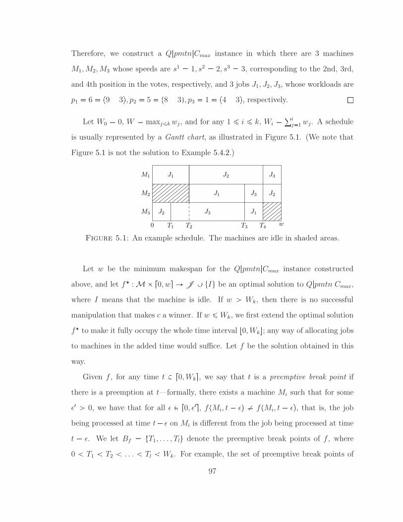
Therefore, we construct a Q|pmtn|Cmax instance in which there are 3 machines
M1, M2, M3 whose speeds are s1 1, s2 2, s3 3, corresponding to the 2nd, 3rd,
and 4th position in the votes, respectively, and 3 jobs J1, J2, J3, whose workloads are
p1 6 p9 3q, p2 5 p8 3q, p3 1 p4 3q, respectively. lLet W0 0, W maxj¤k wj, and for any 1 ¤ i ¤ k, Wi °i
j1 wj. A schedule
is usually represented by a Gantt chart, as illustrated in Figure 5.1. (We note that
Figure 5.1 is not the solution to Example 5.4.2.)
J1 J2 J3
J1 J3 J2
J2 J3 J1
M1
M2
M3
0 T1 T2 T3 T4w
Figure 5.1: An example schedule. The machines are idle in shaded areas.
Let w be the minimum makespan for the Q|pmtn|Cmax instance constructed
above, and let f : M r0, ws ÑJ Y tIu be an optimal solution to Q|pmtn|Cmax,
where I means that the machine is idle. If w ¡ Wk, then there is no successful
manipulation that makes c a winner. If w ¤Wk, we first extend the optimal solution
f to make it fully occupy the whole time interval r0, Wks; any way of allocating jobs
to machines in the added time would suffice. Let f be the solution obtained in this
way.
Given f , for any time t P r0, Wks, we say that t is a preemptive break point if
there is a preemption at t—formally, there exists a machine Mi such that for some
ǫ1 ¡ 0, we have that for all ǫ P r0, ǫ1s, fpMi, t ǫq fpMi, t ǫq, that is, the job
being processed at time t ǫ on Mi is different from the job being processed at time
t ǫ. We let Bf tT1, . . . , Tlu denote the preemptive break points of f , where
0 T1 T2 . . . Tl Wk. For example, the set of preemptive break points of
97
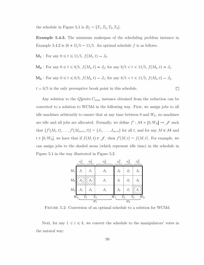
the schedule in Figure 5.1 is Bf tT1, T2, T3, T4u.Example 5.4.3. The minimum makespan of the scheduling problem instance in
Example 5.4.2 is p6 5q5 115. An optimal schedule f is as follows.
M1 : For any 0 ¤ t ¤ 115, fpM1, tq J3.
M2 : For any 0 ¤ t ¤ 85, fpM2, tq J2; for any 85 t ¤ 115, fpM2, tq J1.
M3 : For any 0 ¤ t ¤ 85, fpM3, tq J1; for any 85 t ¤ 115, fpM3, tq J2.
t 85 is the only preemptive break point in this schedule. lAny solution to the Q|pmtn|Cmax instance obtained from the reduction can be
converted to a solution to WCMd in the following way. First, we assign jobs to all
idle machines arbitrarily to ensure that at any time between 0 and Wk, no machines
are idle and all jobs are allocated. Formally, we define f 1 : M r0, Wks Ñ J such
that tf 1pM1, tq, . . . , f 1pMm1, tqu tJ1, . . . , Jm1u for all t, and for any M PM and
t P r0, Wks, we have that if fpM, tq P J , then f 1pM, tq fpM, tq. For example, we
can assign jobs to the shaded areas (which represent idle time) in the schedule in
Figure 5.1 in the way illustrated in Figure 5.2.
J1 J1 J2 J3
J1 J3 J2
J2 J3 J1J3 J3
J2 J2
J1
M1
M2
M3
J3 J2
J1
W0 T1 T2 T3 T4 W2W1
α1
1α1
2α1
3α2
1α2
2α2
3
w1 w2
Figure 5.2: Conversion of an optimal schedule to a solution for WCMd.
Next, for any 1 ¤ i ¤ k, we convert the schedule to the manipulators’ votes in
the natural way:
98
• If there are no preemption break points in pWi1, Wiq, we let manipulator i
vote for c ¡ f 1pM1, Wi1 ǫq ¡ f 1pM2, Wi1 ǫq ¡ . . . ¡ f 1pMm1, Wi1 ǫq,where ǫ ¡ 0 is sufficiently small.
• If there are preemptive break points in pWi1, Wiq, denoted by Ta, Ta1, . . . , Tab1,
then we let V i1 , . . . , V i
b1 denote the orders that correspond to the schedule
at times Wi1 ǫ, Ta ǫ, . . . , Tab1 ǫ, respectively. Let αi1 Ta Wi1,
αi2 Ta1 Ta, . . . , α
ib1 Wi Tab1. We let manipulator i vote for°b1
j1rαijpWi Wi1qs V i
j .
Example 5.4.4. Suppose there are two manipulators whose weights w1 and w2 are
illustrated in Figure 5.2. Manipulator 1 votes rp14qpc ¡ c1 ¡ c3 ¡ c2q p14qpc ¡c1 ¡ c2 ¡ c3q p12qpc ¡ c2 ¡ c1 ¡ c3qs; manipulator 2 votes rp13qpc ¡ c2 ¡ c1 ¡c3q p13qpc ¡ c2 ¡ c3 ¡ c1q p13qpc ¡ c3 ¡ c2 ¡ c1qs. l
On the basis of the exposition above we now refer the reader to Algorithm 1.
The algorithm solves WCMd in three steps: 1. convert the WCMd instance to a
Q|pmtn|Cmax instance; 2. apply a polynomial-time algorithm that solves Q|pmtn|Cmax
(for example, the algorithm in Gonzalez and Sahni (1978)); 3. convert the solution
to the scheduling instance to a solution to the WCMd instance. Algorithm 1 also
solves COd, because the makespan w computed in Line 3 is the optimal solution to
COd. It is easy to verify that the algorithm runs in polynomial time. To conclude,
we have the following result.
Theorem 5.4.5. Algorithm 1 solves WCMd and COd (exactly) in polynomial time.
5.4.2 Algorithm for WCM
We now move on to the more difficult indivisible case. We first note that Algorithm 1
cannot be directly applied to WCM, because the manipulators’ votes constructed in
99

Algorithm 1: compWCMdi ¤ m 1, si ~smp1q si11 i ¤ m 1, pi maxtspP NM , wNM , ciq spP NM , wNM , cq, 0u2
Solve the Q|pmtn|Cmax instance (e.g., by the algorithm in Gonzalez and Sahni3
(1978)). Let w and f denote the minimum makespan and an extendedoptimal schedule; let T1, . . . , Tl denote the preemptive break points.if w ¡ Wk then
4
return false.5
end6
Let f 1 : M r0, Wks ÑJ be such that7 tf 1pM1, tq, . . . , f 1pMm1, tqu tJ1, . . . , Jm1u, and for any M PM, any
t P r0, Wks, we have that if fpM, tq P J , then f 1pM, tq fpM, tq.for i 1 to k do
8
Let V i1 rc ¡ f 1pM1, Wi1 ǫq ¡ . . . ¡ f 1pMm1, Wi1 ǫqs
9
j 210
for each preemptive break point T P pWi1, Wiq (in order) do11
Let V ij rc ¡ f 1pM1, T ǫq ¡ . . . ¡ f 1pMm1, T ǫqs
12
j j 113
end14
For any j, let αij be the length of the jth interval in rWi1, Wis induced by
15
the preemptive break points.Let manipulator i vote
°jrαi
jpWi Wi1qs V ij , and add this vote to P M
16
end17
return P M18
Line 16 can be divisible. For any positional scoring rule, if there is a successful
manipulation (in which all manipulators rank c in the top position), and we increase
the weights of the manipulators, then c still wins the election. This property is
known as monotonicity in weights (see Zuckerman et al. (2009) for a formal definition
and the proof). Therefore, instead of having manipulator i cast the divisible vote°jrαi
jpWi Wi1qs V ij , we let her cast the indivisible vote V i
j, which is one of
the V ij with the highest weight among all the V i
j ’s constructed for manipulator i.
In addition, for any j j, we add one extra manipulator whose weight is αij , and
let the new manipulator vote V ij . It turns out that if we use a particular algorithm
for the scheduling problem, then the solution will not require too many additional
100
manipulators. This gives us Algorithm 2 for WCM.
Algorithm 2: compWCM
This algorithm is the same as Algorithm 1, except for the following two lines:3 Use the algorithm in Gonzalez and Sahni (1978) to solve the schedulingproblem
16 Let manipulator i vote for V ij, where for any j j, αi
j ¥ αij ; and for any
j j, we add a new manipulator whose weight is αij , and let her vote V i
j
Example 5.4.6. Let the coalitional manipulation problem instance be the same as
in Example 5.4.2. Suppose we have two manipulators whose weights are both 1;
then, because the minimum makespan is 115 ¡ 2 (as observed in Example 5.4.3),
there is no solution to the WCMd and WCM problem instances. The solution to the
COd problem instance is 115.
Now suppose we have two manipulators, whose weights are w1 1 and w2 65,
respectively. Let f be the optimal schedule defined in Example 5.4.3. A solution to
the WCMd problem instance is obtained as follows. Manipulator 1 votes rc ¡ c3 ¡c2 ¡ c1s, and manipulator 2 votes rp12qpc ¡ c3 ¡ c2 ¡ c1qp12qpc ¡ c3 ¡ c1 ¡ c2qs.For WCM, the vote of manipulator 1 is the same, the vote of manipulator 2 isrc ¡ c3 ¡ c2 ¡ c1s, and there is one additional manipulator, whose weight is 35 and
whose vote is rc ¡ c3 ¡ c1 ¡ c2s. lExample 5.4.7. Suppose there are two manipulators whose weights are illustrated
in Figure 5.2. The vote of manipulator 1 is c ¡ c2 ¡ c1 ¡ c3, and we introduce
two new manipulators with weight w14 whose votes are c ¡ c1 ¡ c3 ¡ c2 and
c ¡ c1 ¡ c2 ¡ c3. The vote of manipulator 2 is c ¡ c2 ¡ c1 ¡ c3, and we introduce
two new manipulators with weight w23 whose votes are c ¡ c2 ¡ c3 ¡ c1 and
c ¡ c3 ¡ c2 ¡ c1. Since |Bf | (the number of preemptive break points) is 4, there are
in total four additional manipulators. lFor any j j, we must have αi
j ¤ pWi Wi1q2 ¤ W 2 (recall that W 101
maxj¤k wj). Moreover, for any preemptive break point we introduce at most one
extra manipulator. Therefore, we immediately have the following lemma that relates
the number of the new manipulators to the number of preemptive break points.
Lemma 5.4.8. If w ¥ Wk, then there is no successful manipulation for WCMd
(nor for WCM); otherwise, Algorithm 2 returns a manipulation with at most |Bf |additional manipulators, each with weight at most W 2.
Therefore, the smaller |Bf | is, the fewer new manipulators are introduced by
Algorithm 2. |Bf | depends on which algorithm we use to solve Q|pmtn|Cmax in Line 3.
In fact, there are many efficient algorithms that solve Q|pmtn|Cmax. For example,
Q|pmtn|Cmax can be solved in time Opn2mq by a greedy algorithm (Brucker, 2007).
At each time point t, the algorithm (called the level algorithm) assigns jobs to the
machines in a way such that the greater the remaining workload of a job, the faster
the machine it is assigned to.5 However, this algorithm in some cases generates a
schedule that has as many as mpm1q2 preemptive break points. Therefore, we turn
to the algorithm by Gonzalez and Sahni (1978), which runs in time Opn m log nqusing at most 2pm 1q preemptions. Gonzalez and Sahni also showed that this
bound is tight. We note that one preemptive break point corresponds to at least two
preemptions, and in the instances that were used to show that the 2pm1q bound is
tight, m 1 preemptive break points are required. Therefore, we immediately have
the following lemma.
Lemma 5.4.9. The number of preemptive break points in the solution obtained by
the algorithm of Gonzalez and Sahni (1978) is at most m 1. Furthermore, this
bound is tight.
We note that m m 1. Hence, combining Lemma 5.4.8 and Lemma 5.4.9, we
5 The greedy algorithm of Zuckerman et al. (2009) is effectively a discrete-time version of the levelalgorithm.
102

have the following theorem, which is our main result.
Theorem 5.4.10. Algorithm 2 runs in polynomial time and
1. if the algorithm returns false, then there is no successful manipulation (even
for the WCMd version of the instance);
2. otherwise, the algorithm returns a successful manipulation for a modified set
of manipulators, consisting of the original manipulators plus at most m 2
additional manipulators, each with weight at most W 2.5.5 Algorithms for UCM and UCO
We now consider the case where votes are unweighted. UCMd and UCOd can be
solved using Algorithm 1. As for UCM/UCO, every manipulator’s weight is one (so
that W 1), and we are only allowed to add new manipulators whose weight is also
1. We recall that increasing the weights of the manipulators never prevents c from
winning. Therefore, in the context of UCM/UCO we use a slight modification of
Algorithm 2, by adding one unweighted manipulator whenever Algorithm 2 proposes
adding a weighted manipulator (whose weight can be at most 12).
Algorithm 3: compWCM
This algorithm is the same as Algorithm 1, except for the following two lines:3 Use the algorithm in Gonzalez and Sahni (1978) to solve the schedulingproblem.
16 Let manipulator i vote for V i1 ; for any j ¡ 1, we add a new manipulator who
votes for V ij .
The following corollary immediately follows from Theorem 5.4.10.
Corollary 5.5.1. For UCM, if Algorithm 3 returns false, then there is no successful
manipulation; otherwise, Algorithm 3 returns a successful manipulation with at most
m 2 additional manipulators.
103

Recall that Lines 1-3 of Algorithm 3 compute the minimum makespan w (the
solution to COd) of the scheduling problem that is obtained from the UCM instance.
It is easy to see that if votes are divisible then rws is the minimum number of
unweighted manipulators required to make c win the election, that is, rws is the
optimal solution to UCOd. Therefore, Algorithm 1 can easily be modified to yield an
algorithm that solves UCOd. We further note that Algorithm 3 is an approximation
algorithm for UCO, as the number of manipulators returned by Algorithm 3 is no
more than rwsm2. Put another way, Algorithm 3 returns a solution to UCO (with
indivisible votes) that approximates the optimal solution to UCOd (with divisible
votes) to an additive term of m 2.
Generally, if there exists a successful manipulation, then Algorithm 3 returns a
manipulation with additional manipulators. However, there are some special po-
sitional scoring voting rules under which UCM can always be solved exactly by
Algorithm 1. Given l P t1, . . . , m 1u, the l-approval rule is the scoring rule where
~smp1q . . . ~smplq 1 and ~smpl 1q . . . ~smpmq 0. For example, Plu-
rality (with scoring vector p1, 0, . . . , 0q) and Veto (with scoring vector p1, . . . , 1, 0q)are 1-approval and pm 1q-approval, respectively. We note that UCM under any
l-approval rule reduces to the scheduling problem in which all machines have the
same speed. This corresponds exactly to the scheduling problem P |pmtn|Cmax in
discrete time (that is, the preemptions are allowed only at integer time points),
which has a polynomial-time algorithm: Longest Remaining Processing Time first
(LRPT) Pinedo (2008). Therefore, if we modify Algorithm 3 by solving the reduced
scheduling instance with LRPT, then we can solve UCM under any k-approval voting
rule in polynomial time.6 To summarize:
Corollary 5.5.2. Let l P t1, . . . , m 1u. UCM/UCO for l-approval is in P.
6 The simple observation that UCM is in P for approval voting rules was also recently made byAndrew Lin (via personal communication), who employed a completely different (greedy) approach.
104

5.5.1 On The Tightness of The Results
We presently wish to argue that we have made the most of our technique. The next
theorem states that the m 2 bound is tight in terms of the difference between the
optimal solution to UCO and the optimal solution to UCOd under the same input.
It also implies that Algorithm 3 is optimal in the sense that for any q m 2, there
is no approximation algorithm for UCO that always outputs a manipulation with at
most q manipulators more than the optimal solution to UCOd. This result can be
seen as a new type of integrality gap, which applies to our special flavor of rounding.
Theorem 5.5.3. For any m ¥ 3, there exists a UCO instance such that the (additive)
gap between the optimal solution to UCOd and the optimal solution to UCO is m2.
Proof. For any m ¥ 3, we let the scoring vector be pmpm1qpm2q1, . . . , mpm1qpm 2q 1, mpm 1qpm 2q 2, 0q. Let V rc1 ¡ . . . ¡ cm1 ¡ cs, and let
π be the cyclic permutation on Cztcu, that is, π : c1 Ñ . . . Ñ cm1 Ñ c1. For
any i ¤ m 1, let Vi be the linear order over C in which c is ranked in positionpm 1q, and πipc1q ¡Viπipc2q ¡Vi
. . . ¡Viπipcm1q. Let P pV, V1, . . . , Vm1q,
P NM P Y πpP q Y . . .Y πm2pP q. It follows that for any i ¤ m 1, spP NM , ciq spP NM , cq pm 1q2 1. Let V 1 rc ¡ c1 . . . ¡ cm1s; it can be verified that the
divisible vote
1
m 1pV 1, πpV 1q, π2pV 1q, . . . , πm2pV 1qq
is sufficient to make c win, hence the optimal solution to UCOd is 1.
We next prove that the solution to UCO is m 1. Clearly the following profile
is a successful manipulation.pV 1, πpV 1q, π2pV 1q, . . . , πm1pV 1qqHence, it remains to show that the solution is at least m 1. For the sake of
contradiction we assume that the solution is m 2, and P M is the corresponding
105

successful manipulation. Therefore, there must exist i ¤ m 1 such that ci is not
ranked at the bottom of any of the votes of P M . Therefore,
spP M , cq spP M , ciq ¤ m 2 pm 1q2 1,
which means that spP NM Y P M , cq spP NM Y P M , ciq 0. This contradicts the
assumption that P M is a successful manipulation.
We next ask the following natural question: is it possible to improve the rounding
technique so that the algorithm achieves a better bound, relative to the optimal
solution for the indivisible case? This is not ruled out by Theorem 5.5.3, since
that theorem compares to the optimal UCOd solution rather than the optimal UCO
solution. Nevertheless, the answer is negative, as long as all linear orders in an
optimal solution to the COd problem appear in the output of the algorithm. We
say that an approximation algorithm I for UCO is based on COd if for any UCO
instance, there exists an optimal solution to COd such that every linear order that
appears in that solution also appears in the output of I (as a fraction of the vote of
a manipulator).
Theorem 5.5.4. Let I be an approximation algorithm based on COd. For any
m ¥ 3, there exists a UCO instance such that the gap between the optimal solution
to UCO and the output of I is m 2.
Proof. For any m ¥ 3, we construct an instance such that the solution to the UCO
problem is 1, but at least m 1 linear orders appear in any optimal solution to the
COd problem (so the gap is m 2).
We let the scoring vector be pm 2, 1, 0, . . . , 0q. Let
V rc ¡ c1 ¡ . . . ¡ cm1s,and
V 1 rcm1 ¡ c1 ¡ c ¡ c2 ¡ . . . ¡ cm2s.106
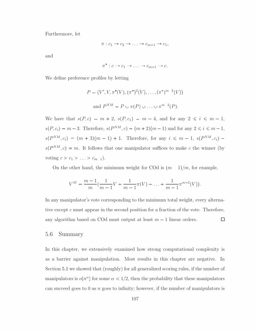
Furthermore, let
π : c1 Ñ c2 Ñ . . .Ñ cm1 Ñ c1,
and
π : c Ñ c1 Ñ . . . Ñ cm1 Ñ c.
We define preference profiles by letting
P pV 1, V, πpV q, pπq2pV q, . . . , pπqm2pV qqand P NM P Y πpP q Y . . .Y πm2pP q.
We have that spP, cq m 2, spP, c1q m 4, and for any 2 ¤ i ¤ m 1,
spP, ciq m 3. Therefore, spP NM , cq pm 2qpm 1q and for any 2 ¤ i ¤ m 1,
spP NM , ciq pm 3qpm 1q 1. Therefore, for any i ¤ m 1, spP NM , ciq spP NM , cq m. It follows that one manipulator suffices to make c the winner (by
voting c ¡ c1 ¡ . . . ¡ cm1).
On the other hand, the minimum weight for COd is pm 1qm, for example,
V M m 1
mp 1
m 1V 1
m 1πpV q . . . 1
m 1πm2pV qq.
In any manipulator’s vote corresponding to the minimum total weight, every alterna-
tive except c must appear in the second position for a fraction of the vote. Therefore,
any algorithm based on COd must output at least m 1 linear orders.
5.6 Summary
In this chapter, we extensively examined how strong computational complexity is
as a barrier against manipulation. Most results in this chapter are negative. In
Section 5.1 we showed that (roughly) for all generalized scoring rules, if the number of
manipulators is opnαq for some α 12, then the probability that these manipulators
can succeed goes to 0 as n goes to infinity; however, if the number of manipulators is
107
ωpnαq for some α ¡ 12, then the probability that these manipulators are all-powerful
goes to 1 as n goes to infinity (except they cannot make alternatives against which
the nonmanipulators are systematically biased win). We note that as n goes to
infinity,?
nn goes to zero.
This “dichotomy” result implies that when the total number of voters is large,
even if the number of manipulators is very small compared to the number of nonma-
nipulators, the manipulators can still manipulate the winner with a high probability.
We further gave an axiomatization in Section 5.3, which tells us how general the class
of GSRs is—it is the class of all voting rules that satisfies anonymity, homogeneity,
and finite local consistency.
Section 5.4 aimed at directly designing (approximation) algorithms for a number
of coalitional manipulation problems for positional scoring rules. Built on top of a
novel connection between coalitional manipulation problems and scheduling prob-
lems, we proposed polynomial-time algorithms that solve WCMd and COd. We also
used these algorithms plus a rounding technique to obtain approximation algorithms
for WCM, UCM, and UCO, with an additive error bound of m 2, which is tight in
a sense.
Therefore, it seems that computational complexity is not a very strong barrier
against manipulation. An obvious next step is to look for other ways to prevent
manipulation. Note that one assumption made in all previous manipulation settings
is that the manipulators have full information about the votes of the nonmanipu-
lators. Therefore, a natural question to ask is: What if the manipulators do not
have full information about the other voters’ votes? The work in the next chapter is
motivated by this question. We will study the case of one manipulator with limited
information about other voters’ votes. We will prove that restricting the information
of the manipulator can effectively make a certain type of manipulation, which we
call dominating manipulation, NP-hard. At one extreme, if the manipulator knows
108

nothing, many voting rules are immune to dominating manipulations. These results
seem very natural at a high level, but to obtain them, we need a formal model to
analyze voters’ strategic behavior.
109
6
Preventing Manipulation by Restricting
Information
It was shown in the last chapter that computational complexity does not seem to be
a very strong barrier against manipulation. Consequently, we need to look for new
barriers. In this chapter we examine some preliminary ideas to prevent manipula-
tion for the cases where there is one manipulator, by restricting the manipulator’s
information about the other voters’ votes. We recall that in all previously studied
manipulation problems, it is normally assumed that the manipulator has full infor-
mation about the votes of the non-manipulators. The argument often given is that
if it is NP-hard with full information, then it only can be at least as computationally
difficult with partial information. However, when there is only one manipulator,
computing a manipulation is in P for most common voting rules, including all posi-
tional scoring rules, Copeland, maximin, and voting trees (see Table 3.1). The only
known exceptions are STV (Bartholdi and Orlin, 1991), ranked pairs (Xia et al.,
2009), and Nanson’s and Baldwin’s rules (Narodytska et al., 2011). It is not clear
whether it is computationally easy for a single manipulator to find a manipulation
when she only has partial information for other rules.
110

In this chapter, we first model how one manipulator computes a manipulation
based on partial information about the other votes. For example, the manipulator
may know that some voters prefer one alternative to another, but might not be able
to know all pairwise comparisons for all voters. We suppose the knowledge of the
manipulator is described by an information set E. This is some subset of possible
profiles of the non-manipulators which is known to contain the true profile. Given an
information set and a pair of votes U and V , if for every profile in E, the manipulator
is not worse off voting U than voting V , and there exists a profile in E such that
the manipulator is strictly better off voting U , then we say that U dominates V . If
there exists a vote U that dominates the true preferences of the manipulator then
the manipulator has an incentive to vote untruthfully. We call this a dominating
manipulation. If there is no such vote, then a cautious manipulator might have little
incentive to vote strategically.
We are interested in whether a voting rule r is immune to dominating manipula-
tions, meaning that a voter’s true preferences are never dominated by another vote.
If r is not immune to dominating manipulations, we are interested in whether r is
resistant, meaning that computing whether a voter’s true preferences are dominated
by another vote U is NP-hard, or vulnerable, meaning that this problem is in P. These
properties depend on both the voting rule and the form of the partial information.
Interestingly, it is not hard to see that most voting rules are immune to manipu-
lation when the partial information is just the current winner. For instance, with
any majority consistent rule (for example, plurality), a risk averse manipulator will
still want to vote for her most preferred alternative. This means that the chairman
does not need to keep the current winner secret to prevent such manipulations. On
the other hand, if the chairman lets slip more information, many rules stop being
immune. With most scoring rules, if the manipulator knows the current scores, then
the rule is no longer immune to such manipulation. For instance, when her most
111

preferred alternative is too far behind to win, the manipulator might vote instead
for a less preferred candidate who can win.
In this chapter, we focus on the case where the partial information is represented
by a profile Ppo of partial orders, and the information set E consists of all linear
orders that extend Ppo. The dominating manipulation problem is related to the pos-
sible/necessary winner problems, which I have briefly talked about in Section 1.6 and
Section 2.3. We recall that in possible/necessary winner problems, we are given an
alternative c and a profile of partial orders Ppo that represents the partial information
of the voters’ preferences. We are asked whether c is the winner for some extension of
Ppo (that is, c is a possible winner), or whether c is the winner for every extension of
Ppo (that is, c is a necessary winner). We note that in the possible/necessary winner
problems, there is no manipulator and Ppo represents the chair’s partial information
about the votes. In dominating manipulation problems, Ppo represents the partial
information of the manipulator about the non-manipulators.
In the following sections, we start with the special case where the manipulator
has complete information. In this setting the dominating manipulation problem
reduces to the standard manipulation problem, and many common voting rules are
vulnerable to dominating manipulation (from known results). When the manipulator
has no information, we show that a wide range of common voting rules are immune to
dominating manipulation. When the manipulator’s partial information is represented
by partial orders, our results are summarized in Table 6.1.
Our results are encouraging. For most voting rules r we study in this paper
(except plurality and veto), hiding even a little information makes r resistant to
dominating manipulation. If we hide all information, then r is immune to dominat-
ing manipulation. Therefore, limiting the information available to the manipulator
1 All hardness results hold even when the number of undetermined pairs in each partial order isno more than a constant.
112
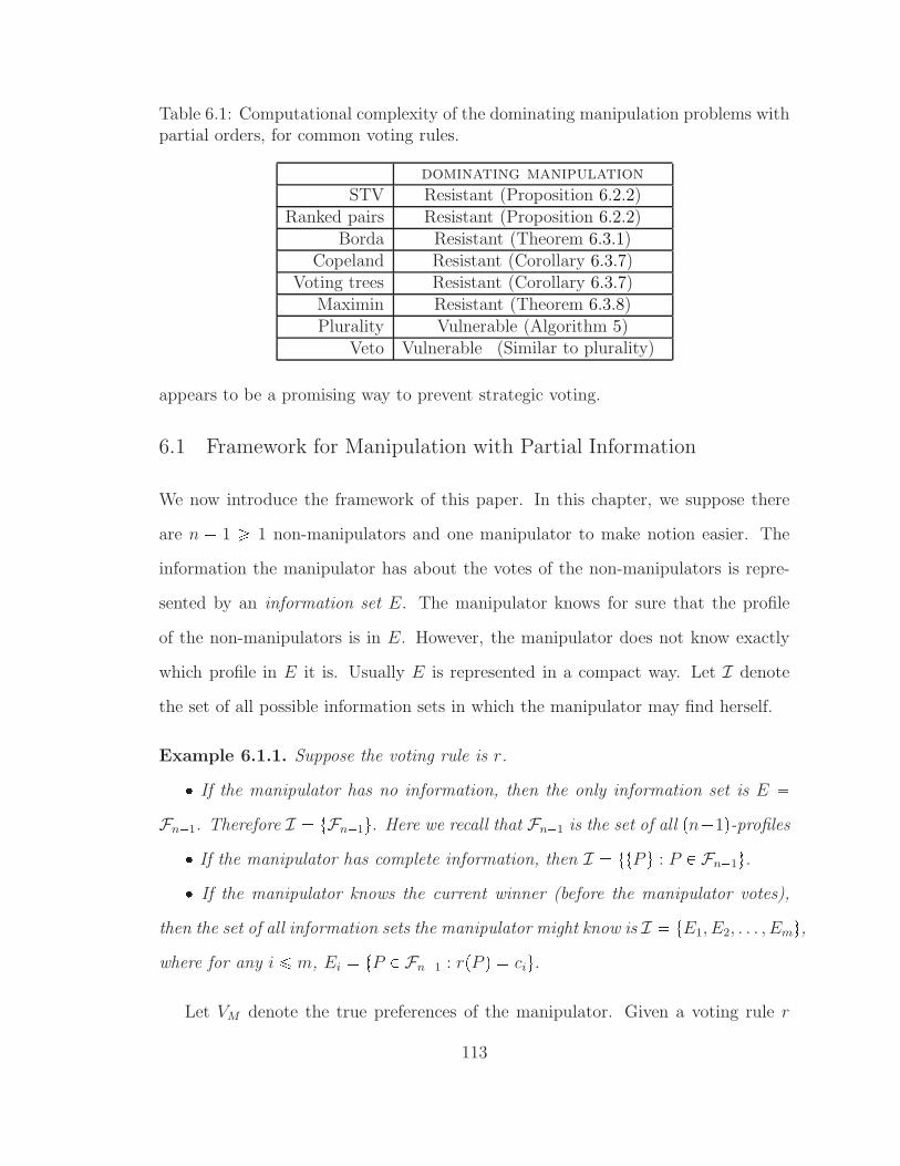
Table 6.1: Computational complexity of the dominating manipulation problems withpartial orders, for common voting rules.
dominating manipulationSTV Resistant (Proposition 6.2.2)
Ranked pairs Resistant (Proposition 6.2.2)Borda Resistant (Theorem 6.3.1)
Copeland Resistant (Corollary 6.3.7)Voting trees Resistant (Corollary 6.3.7)
Maximin Resistant (Theorem 6.3.8)Plurality Vulnerable (Algorithm 5)
Veto Vulnerable (Similar to plurality)
appears to be a promising way to prevent strategic voting.
6.1 Framework for Manipulation with Partial Information
We now introduce the framework of this paper. In this chapter, we suppose there
are n 1 ¥ 1 non-manipulators and one manipulator to make notion easier. The
information the manipulator has about the votes of the non-manipulators is repre-
sented by an information set E. The manipulator knows for sure that the profile
of the non-manipulators is in E. However, the manipulator does not know exactly
which profile in E it is. Usually E is represented in a compact way. Let I denote
the set of all possible information sets in which the manipulator may find herself.
Example 6.1.1. Suppose the voting rule is r. If the manipulator has no information, then the only information set is E Fn1. Therefore I tFn1u. Here we recall that Fn1 is the set of all pn1q-profiles If the manipulator has complete information, then I ttP u : P P Fn1u. If the manipulator knows the current winner (before the manipulator votes),
then the set of all information sets the manipulator might know is I tE1, E2, . . . , Emu,where for any i ¤ m, Ei tP P Fn1 : rpP q ciu.
Let VM denote the true preferences of the manipulator. Given a voting rule r
113

and an information set E, we say that a vote U dominates another vote V , if for
every profile P P E, we have rpP Y tUuq ©VMrpP Y tV uq, and there exists P 1 P E
such that rpP 1Y tUuq ¡VMrpP 1Y tV uq. In other words, when the manipulator only
knows the voting rule r and the fact that the profile of the non-manipulators is in
E (and no other information), voting U is a strategy that dominates voting V . We
define the following two decision problems.
Definition 6.1.2. Given a voting rule r, an information set E, the true preferences
VM of the manipulator, and two votes V and U , we are asked the following two ques-
tions. Does U dominate V ? This is the domination problem. Does there exist a vote V 1 that dominates VM? This is the dominating manipu-
lation problem.
We stress that usually E is represented in a compact way, otherwise the input
size would already be exponentially large, which would trivialize the computational
problems. Given a set I of information sets, we say a voting rule r is immune to
dominating manipulation, if for every E P I and every VM that represents the ma-
nipulator’s preferences, VM is not dominated; r is resistant to dominating manipula-
tion, if dominating manipulation is NP-hard (which means that r is not immune
to dominating manipulation, assuming PNP); and r is vulnerable to dominating
manipulation, if r is not immune to dominating manipulation, and dominating
manipulation is in P.
6.2 Manipulation with Complete/No Information
In this section we focus on the following two special cases: (1) the manipulator has
complete information, and (2) the manipulator has no information. It is not hard to
see that when the manipulator has complete information, dominating manipula-
114
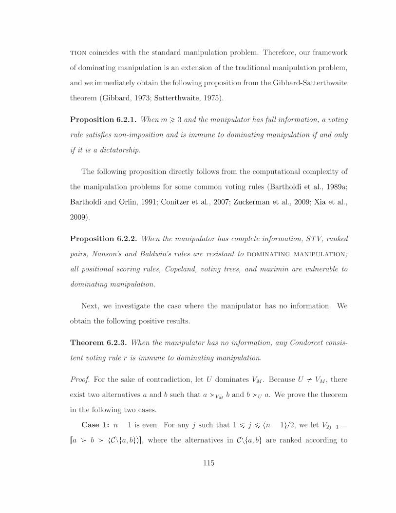
tion coincides with the standard manipulation problem. Therefore, our framework
of dominating manipulation is an extension of the traditional manipulation problem,
and we immediately obtain the following proposition from the Gibbard-Satterthwaite
theorem (Gibbard, 1973; Satterthwaite, 1975).
Proposition 6.2.1. When m ¥ 3 and the manipulator has full information, a voting
rule satisfies non-imposition and is immune to dominating manipulation if and only
if it is a dictatorship.
The following proposition directly follows from the computational complexity of
the manipulation problems for some common voting rules (Bartholdi et al., 1989a;
Bartholdi and Orlin, 1991; Conitzer et al., 2007; Zuckerman et al., 2009; Xia et al.,
2009).
Proposition 6.2.2. When the manipulator has complete information, STV, ranked
pairs, Nanson’s and Baldwin’s rules are resistant to dominating manipulation;
all positional scoring rules, Copeland, voting trees, and maximin are vulnerable to
dominating manipulation.
Next, we investigate the case where the manipulator has no information. We
obtain the following positive results.
Theorem 6.2.3. When the manipulator has no information, any Condorcet consis-
tent voting rule r is immune to dominating manipulation.
Proof. For the sake of contradiction, let U dominates VM . Because U VM , there
exist two alternatives a and b such that a ¡VMb and b ¡U a. We prove the theorem
in the following two cases.
Case 1: n 1 is even. For any j such that 1 ¤ j ¤ pn 1q2, we let V2j1 ra ¡ b ¡ pCzta, buqs, where the alternatives in Czta, bu are ranked according to
115

the ascending order of their subscripts; let V2j rb ¡ a ¡ RevpCzta, buqs. Here
RevpCzta, buq is the reverse of Czta, bu. Let P pV1, . . . , Vn1xq. It follows that a
is the Condorcet winner for P Y tVMu and b is the Condorcet winner for P Y tUu.Because a ¡VM
b, VM is not dominated by U , which contradicts the assumption.
Case 2: n 1 is odd. For any j such that 1 ¤ j ¤ pn 2q2, we let V2j1 ra ¡b ¡ pCzta, buqs and V2j rb ¡ a ¡ RevpCzta, buqs. Suppose a ci1 and b ci2 . Let
Vn1 " V1 if i1 ¡ i2V2 if i1 i2
. Let P pV1, . . . , Vn1q. It follows that a is the Condorcet
winner for P Y tVMu and b is the Condorcet winner for P Y tUu, which contradicts
the assumption.
Theorem 6.2.4. When the manipulator has no information, Borda is immune to
dominating manipulation.
Proof. For the sake of contradiction, let U dominates VM . Because U VM , there
exists i ¤ m such that AltpVM , iq AltpU, iq and for every i i, AltpVM , iq AltpU, iq. That is, i is the first position from the top where the alternatives in VM
and U are different. Let ci1 AltpVM , iq and ci2 AltpUM , iq. We prove the
theorem in the following three cases.
Case 1: n 1 is even. For any i i1 ¤ m, let Vri,i1sM denote the sub-linear-order
of VM that starts at the ith position of VM and ends at the i1th position of VM .
For any j such that 1 ¤ j ¤ pn 1q2, we let V2j1 rV ri,msM ¡ RevpV r1,i1sq
M sand V2j rRevpV ri,ms
M q ¡ RevpV r1,i1sqM s. Let P pV1, . . . , Vn1q. It follows that
BordapP Y tVMuq ci1 and BordapP Y tUuq ci2. We note that ci1 ¡VMci2 , which
contradicts the assumption.
Case 2: n 1 is odd and c1 is ranked within top i positions in VM . For
any j such that 1 ¤ j ¤ pn 2q2, we let V2j1 rc1 ¡ c2 ¡ ¡ cms and
V2j rcm ¡ cm1 ¡ ¡ c1s. Let Vn1 RevpV q and P pV1, . . . , Vn1q. It
116

follows that BordapP Y tV uq c1 and BordapP Y tUuq c1, which contradicts the
assumption.
Case 3: n 1 is odd and c1 is not ranked within top i positions in VM . Let
V1, . . . , Vn2 be defined the same as in Case 2. Let V 1 rV ri,msM ¡ RevpV r1,i1s
M qs.Let U 1 rU ri,ms ¡ RevpU r1,i1sqs. It follows that BordapV 1, VMq ci1 . Let
a BordapV 1, Uq. If a ci1 , then ci1 ¡VMa. This is because the alternatives
ranked within top i 1 positions in VM gets exactly the average score in tV 1, Uu,which means that in order for any of them to win, the scores of all alternative
in tV 1, Uu must be the same. However, due to the tie-breaking mechanism, the
winner is c1, which contradicts the assumption that c1 is not ranked within top ipositions in VM . Let P 1 pV1, . . . , Vn2, V
1q, we have that BordapP 1 Y tVMuq ci1 ¡VM
a BordapP 1 Y tUuq, which contradicts the assumption. If a ci1, then
BordapU 1, VMq BordapV 1, Uq a ci1 . Let P pV1, . . . , Vn2, U1q. We have
BordapP Y tVMuq ci1 ¡VMci2 BordapP Y tUuq, which is a contradiction.
Therefore, the theorem is proved.
Theorem 6.2.5. When the manipulator has no information and n ¥ 6pm 2q 1,
any positional scoring rule is immune to dominating manipulation.
Proof. For the sake of contradiction, let U dominates VM . Let c arg maxct~smpVM , cq :
~smpVM , cq ¡ ~smpU, cqu. It follows that there exists an alternative c1 such that
~smpVM , c1q ~smpVM , cq and ~smpU, c1q ~smpVM , cq. It follows that smpVM , cq ¡~smpVM , c1q and ~smpU, c1q ~smpVM , cq ¡ ~smpU, cq.
We prove the theorem for the case where c c1 and c1 c2. The other cases
can be proved similarly. Let Mm2 denote the cyclic permutation such that c3 Ñc4 Ñ Ñ cm Ñ c3. For any k P N and any c P Cztc1, c2u, we let M0
m2pcq c and
Mkm2pcq MpMk1
m2pcqq. Let W rc1 ¡ c2 ¡ c3 ¡ ¡ cms and W 1 rc2 ¡ c1 ¡c3 ¡ ¡ cms. Let P1 denote the 6pm 2q-profile that is composed of three copies
117
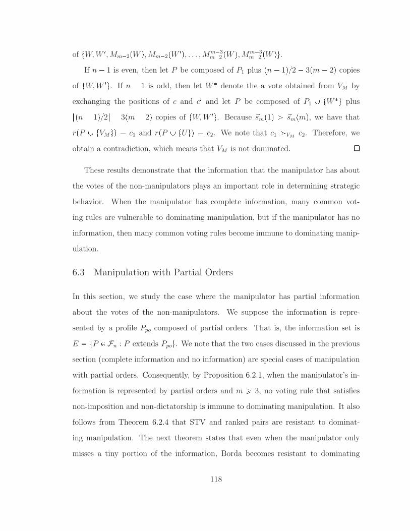
of tW, W 1, Mm2pW q, Mm2pW 1q, . . . , Mm3m2 pW q, Mm3
m2 pW qu.If n 1 is even, then let P be composed of P1 plus pn 1q2 3pm 2q copies
of tW, W 1u. If n 1 is odd, then let W denote the a vote obtained from VM by
exchanging the positions of c and c1 and let P be composed of P1 Y tW u plustpn 1q2u 3pm 2q copies of tW, W 1u. Because ~smp1q ¡ ~smpmq, we have that
rpP Y tVMuq c1 and rpP Y tUuq c2. We note that c1 ¡VMc2. Therefore, we
obtain a contradiction, which means that VM is not dominated.
These results demonstrate that the information that the manipulator has about
the votes of the non-manipulators plays an important role in determining strategic
behavior. When the manipulator has complete information, many common vot-
ing rules are vulnerable to dominating manipulation, but if the manipulator has no
information, then many common voting rules become immune to dominating manip-
ulation.
6.3 Manipulation with Partial Orders
In this section, we study the case where the manipulator has partial information
about the votes of the non-manipulators. We suppose the information is repre-
sented by a profile Ppo composed of partial orders. That is, the information set is
E tP P Fn : P extends Ppou. We note that the two cases discussed in the previous
section (complete information and no information) are special cases of manipulation
with partial orders. Consequently, by Proposition 6.2.1, when the manipulator’s in-
formation is represented by partial orders and m ¥ 3, no voting rule that satisfies
non-imposition and non-dictatorship is immune to dominating manipulation. It also
follows from Theorem 6.2.4 that STV and ranked pairs are resistant to dominat-
ing manipulation. The next theorem states that even when the manipulator only
misses a tiny portion of the information, Borda becomes resistant to dominating
118

manipulation.
Theorem 6.3.1. domination and dominating manipulation with partial orders
are NP-hard for Borda, even when the number of unknown pairs in each vote is no
more than 4.
Proof. We only prove that domination is NP-hard, via a reduction from Exact
Cover by 3-Sets (x3c). The proof for dominating manipulation is similar
to the proof of the NP-hardness of the possible winner problems under positional
scoring rules in Xia and Conitzer (2011a).
In an x3c instance, we are given two sets V tv1, . . . , vqu, S tS1, . . . , Stu,where for any j ¤ t, Sj V and |Sj| 3. We are asked whether there exists a
subset S 1 of S such that each element in V is in exactly one of the 3-sets in S 1. We
construct a domination instance as follows.
Alternatives: C tc, w, du Y V, where d is an auxiliary alternative. Therefore,
m |C| q 3. Ties are broken in the following order: c ¡ w ¡ V ¡ d.
Manipulator’s preferences and possible manipulation: VM rw ¡ c ¡ d ¡Vs. We are asked whether V VM is dominated by U rw ¡ d ¡ c ¡ Vs.The profile of partial orders: Let Ppo P1 Y P2, defined as follows.
First part (P1) of the profile: For each j ¤ t, We define a partial order Oj as
follows.
Oj rw ¡ Sj ¡ d ¡ Othersszrtwu pSj Y tduqsThat is, Oj is a partial order that agrees with w ¡ Sj ¡ d ¡ Others, except that
the pairwise relations between pw, Sjq and pw, dq are not determined (and these are
the only 4 unknown relations). Let P1 tO1, . . . , Otu.Second part (P2) of the profile: We first give the properties that we need P2
to satisfy, then show how to construct P2 in polynomial time. All votes in P2 are
linear orders that are used to adjust the score differences between alternatives. Let
119

P 11 tw ¡ Si ¡ d ¡ Others : i ¤ tu. That is, P 11 (|P 11| t) is an extension of P1 (in
fact, P 11 is the set of linear orders that we started with to obtain P1, before removing
some of the pairwise relations). Let ~sm pm 1, . . . , 0q. P2 is a set of linear orders
such that the following holds for Q P 11 Y P2 Y tV u:(1) For any i ¤ q, ~smpQ, cq ~smpQ, viq 1, ~smpQ, wq ~smpQ, cq 4q3.
(2) For any i ¤ q, the scores of vi and w, c are higher than the score of d in any
extension of P1 Y P2 Y tV u and in any extension of P1 Y P2 Y tUu.(3) The size of P2 is polynomial in t q.
We now show how to construct P2 in polynomial time. For any alternative a d,
we define the following two votes: Wa tra ¡ d ¡ Otherss, rRevpOthersq ¡ a ¡ dsu,where RevpOthersq is the reversed order of the alternatives in Czta, du. We note that
for any alternative a1 P Czta, du, ~smpW, aq~smpW, a1q 1 and ~smpW, a1q~smpW, dq 1. Let Q1 P 11 Y tV u. P2 is composed of the following parts:
(1) tm ~smpQ1, cq copies of Wc.
(2) tm 4q3 ~smpQ1, wq copies of Ww.
(2) For each i ¤ q, there are tm 1 ~smpQ1, viq copies of Wvi.
We next prove that V is dominated by U if and only if c is the winner in at least
one extension of Ppo Y tV u. We note that for any v P V Y twu, the score of v in V
is the same as the score of v in U . The score of c in U is lower than the score of
c in V . Therefore, for any extension P of Ppo, if rpP Y tV uq P ptwu Y Vq, then
rpP Y tV uq rpP Y tUuq (because d cannot win). Hence, for any extension P of
Ppo, voting U can result in a different outcome than voting V only if rpP Y V q c.
If there exists an extension P of Ppo such that rpP Y tV uq c, then we claim
that the manipulator is strictly better off voting U than voting V . Let P 1 denote
the extension of P1 in P . Then, because the total score of w is no more than the
total score of c, w is ranked lower than d at least q
3times in P 1 . Meanwhile, for each
i ¤ q, vi is not ranked higher than w more than one time in P 1 , because otherwise
120
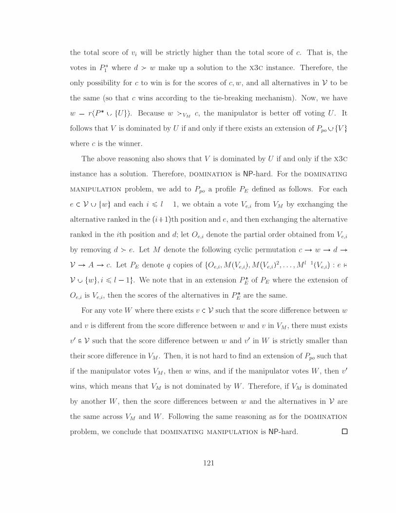
the total score of vi will be strictly higher than the total score of c. That is, the
votes in P 1 where d ¡ w make up a solution to the x3c instance. Therefore, the
only possibility for c to win is for the scores of c, w, and all alternatives in V to be
the same (so that c wins according to the tie-breaking mechanism). Now, we have
w rpP Y tUuq. Because w ¡VMc, the manipulator is better off voting U . It
follows that V is dominated by U if and only if there exists an extension of PpoYtV uwhere c is the winner.
The above reasoning also shows that V is dominated by U if and only if the x3c
instance has a solution. Therefore, domination is NP-hard. For the dominating
manipulation problem, we add to Ppo a profile PE defined as follows. For each
e P V Y twu and each i ¤ l 1, we obtain a vote Ve,i from VM by exchanging the
alternative ranked in the pi1qth position and e, and then exchanging the alternative
ranked in the ith position and d; let Oe,i denote the partial order obtained from Ve,i
by removing d ¡ e. Let M denote the following cyclic permutation c Ñ w Ñ d ÑV Ñ A Ñ c. Let PE denote q copies of tOe,i, MpVe,iq, MpVe,iq2, . . . , M l1pVe,iq : e PV Y twu, i ¤ l 1u. We note that in an extension P E of PE where the extension of
Oe,i is Ve,i, then the scores of the alternatives in P E are the same.
For any vote W where there exists v P V such that the score difference between w
and v is different from the score difference between w and v in VM , there must exists
v1 P V such that the score difference between w and v1 in W is strictly smaller than
their score difference in VM . Then, it is not hard to find an extension of Ppo such that
if the manipulator votes VM , then w wins, and if the manipulator votes W , then v1wins, which means that VM is not dominated by W . Therefore, if VM is dominated
by another W , then the score differences between w and the alternatives in V are
the same across VM and W . Following the same reasoning as for the domination
problem, we conclude that dominating manipulation is NP-hard.
121
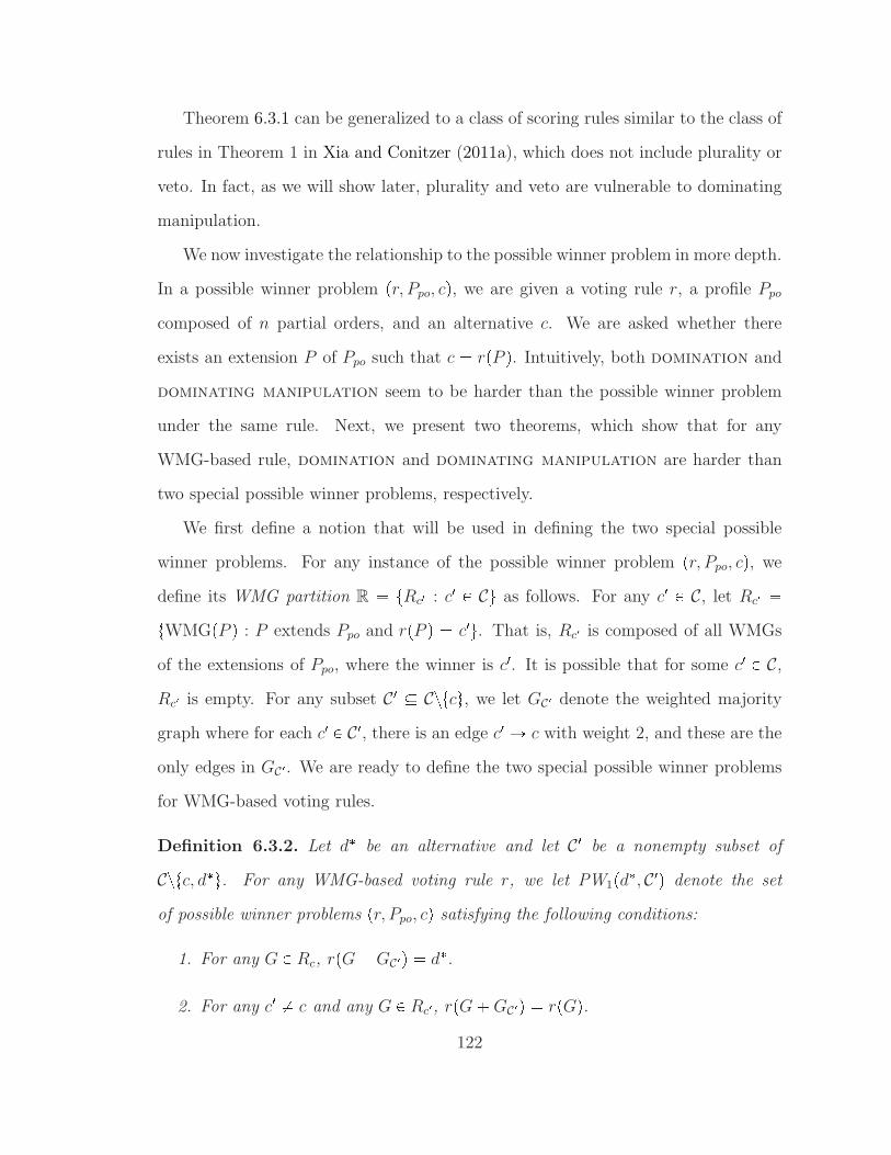
Theorem 6.3.1 can be generalized to a class of scoring rules similar to the class of
rules in Theorem 1 in Xia and Conitzer (2011a), which does not include plurality or
veto. In fact, as we will show later, plurality and veto are vulnerable to dominating
manipulation.
We now investigate the relationship to the possible winner problem in more depth.
In a possible winner problem pr, Ppo, cq, we are given a voting rule r, a profile Ppo
composed of n partial orders, and an alternative c. We are asked whether there
exists an extension P of Ppo such that c rpP q. Intuitively, both domination and
dominating manipulation seem to be harder than the possible winner problem
under the same rule. Next, we present two theorems, which show that for any
WMG-based rule, domination and dominating manipulation are harder than
two special possible winner problems, respectively.
We first define a notion that will be used in defining the two special possible
winner problems. For any instance of the possible winner problem pr, Ppo, cq, we
define its WMG partition R tRc1 : c1 P Cu as follows. For any c1 P C, let Rc1 tWMGpP q : P extends Ppo and rpP q c1u. That is, Rc1 is composed of all WMGs
of the extensions of Ppo, where the winner is c1. It is possible that for some c1 P C,
Rc1 is empty. For any subset C1 Cztcu, we let GC1 denote the weighted majority
graph where for each c1 P C1, there is an edge c1 Ñ c with weight 2, and these are the
only edges in GC1 . We are ready to define the two special possible winner problems
for WMG-based voting rules.
Definition 6.3.2. Let d be an alternative and let C1 be a nonempty subset of
Cztc, du. For any WMG-based voting rule r, we let PW1pd, C1q denote the set
of possible winner problems pr, Ppo, cq satisfying the following conditions:
1. For any G P Rc, rpGGC1q d.2. For any c1 c and any G P Rc1, rpGGC1q rpGq.
122
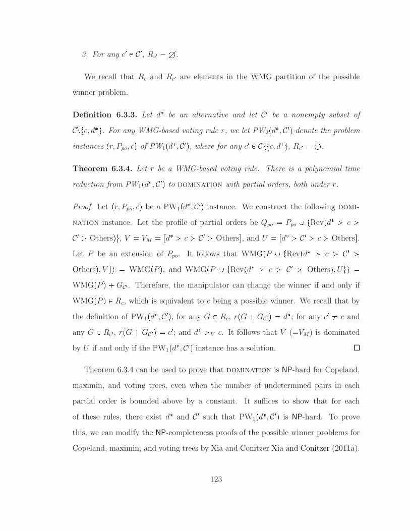
3. For any c1 P C1, Rc1 H.
We recall that Rc and Rc1 are elements in the WMG partition of the possible
winner problem.
Definition 6.3.3. Let d be an alternative and let C1 be a nonempty subset of
Cztc, du. For any WMG-based voting rule r, we let PW2pd, C1q denote the problem
instances pr, Ppo, cq of PW1pd, C1q, where for any c1 P Cztc, du, Rc1 H.
Theorem 6.3.4. Let r be a WMG-based voting rule. There is a polynomial time
reduction from PW1pd, C1q to domination with partial orders, both under r.
Proof. Let pr, Ppo, cq be a PW1pd, C1q instance. We construct the following domi-
nation instance. Let the profile of partial orders be Qpo Ppo Y tRevpd ¡ c ¡C1 ¡ Othersqu, V VM rd ¡ c ¡ C1 ¡ Otherss, and U rd ¡ C1 ¡ c ¡ Otherss.Let P be an extension of Ppo. It follows that WMGpP Y tRevpd ¡ c ¡ C1 ¡Othersq, V uq WMGpP q, and WMGpP Y tRevpd ¡ c ¡ C1 ¡ Othersq, Uuq WMGpP q GC1. Therefore, the manipulator can change the winner if and only if
WMGpP q P Rc, which is equivalent to c being a possible winner. We recall that by
the definition of PW1pd, C1q, for any G P Rc, rpG GC1q d; for any c1 c and
any G P Rc1, rpG GC1q c1; and d ¡V c. It follows that V (=VM) is dominated
by U if and only if the PW1pd, C1q instance has a solution.
Theorem 6.3.4 can be used to prove that domination is NP-hard for Copeland,
maximin, and voting trees, even when the number of undetermined pairs in each
partial order is bounded above by a constant. It suffices to show that for each
of these rules, there exist d and C1 such that PW1pd, C1q is NP-hard. To prove
this, we can modify the NP-completeness proofs of the possible winner problems for
Copeland, maximin, and voting trees by Xia and Conitzer Xia and Conitzer (2011a).
123

Corollary 6.3.5. domination with partial orders is NP-hard for Copeland, max-
imin, and voting trees, even when the number of unknown pairs in each vote is
bounded above by a constant.
Proof. Copeland: We tweak the reduction in the NP-completeness proof of PW
w.r.t. Copeland (Xia and Conitzer, 2011a, Theorem 3) by letting Dpc, vq 1 for any
alternative v P V and use the tie-breaking mechanism where w ¡ c ¡ Others. Let
d w, C1 B, V U rw ¡ c ¡ C1 ¡ Otherss and W rw ¡ C1 ¡ c ¡ Otherss.It follows that the alternatives in B never wins the elections, and if c wins the election
in an extension P of Ppo, then the Copeland score of c is 8t 1 and the Copeland
score of w 8t. However, in the weighted majority graph WMGpP q GC1, c loses
to all alternatives in C1 in their pairwise elections, which means that the Copeland
score of c is t 1. Consequently w is the winner. On the other hand, for any
extension P where c is not the winner, w is the winner, and w is also the winner
in the weighted majority graph WMGpP q GC1. Therefore, the PW instance is a
PW1pd, C1q instance.
Maximin: We tweak the reduction in the NP-completeness proof of PW w.r.t. max-
imin (Xia and Conitzer, 2011a, Theorem 5) by letting Dpw1, wq t. Let d w,
C1 tw1u, V U rw ¡ c ¡ w1 ¡ Vs and W rw ¡ w1 ¡ c ¡ Vs. We adopt the
tie-breaking mechanism where w ¡ c ¡ V ¡ w1. It is easy to check that w1 never
wins the elections. If c wins the election in an extension P of Ppo, then the minimum
pairwise score of c is t2, and the minimum pairwise score of w and the alternatives
in V are t. We note that in the majority graph WMGpP qGC1, the minimum pair-
wise score of c is t (against w1), which means that rpWMGpP qGC1q w. For any
extension P of Ppo such that rpP q c, it easy to check that the winner is in twuYV,
and the minimum pairwise scores of them are the same as in the weighted majority
graph WMGpP q GC1. Therefore, the PW instance is a PW1pd, C1q instance.
124

Voting trees: We tweak the reduction in the NP-completeness proof of PW
w.r.t. voting trees (Xia and Conitzer, 2011a, Theorem 7) by letting Dpc, dq 1. Let
d w, C1 tdu, V U rw ¡ c ¡ d ¡ Otherss and W rw ¡ d ¡ c ¡ Otherss.For any extension P of Ppo where c wins, the winner for the weighted majority
graph WMGpP q GC1 is w, because c loses to d in the first round, and w beats any
other alternatives (except c) in their pairwise elections. For any extension P of Ppo
where c does not win, the winner is w. Therefore, the PW instance is a PW1pd, C1qinstance.
Theorem 6.3.6. Let r be a WMG-based voting rule. There is a polynomial-time
reduction from PW2pd, C1q to dominating manipulation with partial orders, both
under r.
Proof. The proof is similar to the proof for Theorem 6.3.4. We note that d is the
manipulator’s top-ranked alternative. Therefore, if c is not a possible winner, then
V ( VM) is not dominated by any other vote; if c is a possible winner, then V is
dominated by U rw ¡ C1 ¡ c ¡ Otherss.Similarly, we have the following corollary.
Corollary 6.3.7. dominating manipulation with partial orders is NP-hard for
Copeland and voting trees, even when the number of unknown pairs in each vote is
bounded above by a constant.
It is an open question if PW2pd, C1q with partial orders is NP-hard for maximin.
However, we can directly prove that dominating manipulation is NP-hard for
maximin by a reduction from x3c.
Theorem 6.3.8. dominating manipulation with partial orders is NP-hard for
maximin, even when the number of unknown pairs in each vote is no more than 4.
125

Proof. We prove the hardness result by a reduction from x3c. Given an x3c instance
V tv1, . . . , vqu, S tS1, . . . , Stu, where q t ¡ 3, we construct a dominating
manipulation instance as follows.
Alternatives: V Y tc, w, w1u. Ties are broken in the order w ¡ V ¡ c ¡ w1.First part P1 of the profile: for each i ¤ t, we start with the linear order Vi rw ¡ Si ¡ c ¡ pVzSiq ¡ w1s, and subsequently obtain a partial order Oi by removing
the relations in twupSiYtcuq. For each i ¤ t, we let O1i be a partial order obtained
from V 1i rw ¡ vi ¡ Otherss by removing w ¡ vi. We let O1 be a partial order
obtained from V 1 rw1 ¡ w ¡ Otherss by removing w1 ¡ w. Let P1 be the profile
composed of tO1, . . . , Otu, 2 copies of tO11, . . . , O
1tu, and 3 copies of O1. Let P 11 denote
the extension of P1 that consists of V1, . . . , Vt, 2 copies of tV 11 , . . . , V
1t u, and 3 copies
of V 1.Second part P2 of the profile: P2 is defined to be a a set of linear orders such
that the pairwise score differences of P 11 Y P2 Y tV u satisfy:
(1) Dpw, cq 2t 2q
3, Dpw1, wq 2t 6, Dpw1, cq 2t, and for all i ¤ q,
Dpw, viq 2t 4 and Dpvi, w1q 4pt qq.
(2) Dpl, rq ¤ 1 for all other pairwise scores not defined in (1).
Manipulator’s preferences: VM rw ¡ V ¡ c ¡ w1s.We note that in any extension of P1YP2, after the manipulator changes her vote
from VM to rw ¡ V ¡ w1 ¡ cs, the only change made to the weighted majority graph
is that the weight on w Ñ c increases by 2. Since w1 never wins in any extension, if
c does not win when the manipulator votes for VM , then the winner does not change
after the manipulator changes her vote to rw ¡ V ¡ w1 ¡ cs. It follows from the proof
of Theorem 6.3.4, Corollary 6.3.5, and Theorem 5 in Xia and Conitzer (2011a) that
if the x3c instance has a solution, then VM is dominated by U rw ¡ V ¡ w1 ¡ cs.126
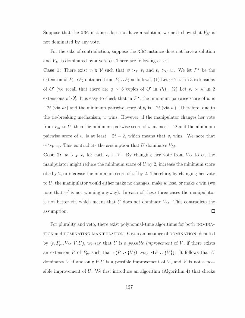
Suppose that the x3c instance does not have a solution, we next show that VM is
not dominated by any vote.
For the sake of contradiction, suppose the x3c instance does not have a solution
and VM is dominated by a vote U . There are following cases.
Case 1: There exist vi P V such that w ¡V vi and vi ¡U w. We let P be the
extension of P1YP2 obtained from P 11YP2 as follows. (1) Let w ¡ w1 in 3 extensions
of O1 (we recall that there are q ¡ 3 copies of O1 in P1). (2) Let vi ¡ w in 2
extensions of O1i. It is easy to check that in P , the minimum pairwise score of w is2t (via w1) and the minimum pairwise score of vi is 2t (via w). Therefore, due to
the tie-breaking mechanism, w wins. However, if the manipulator changes her vote
from VM to U , then the minimum pairwise score of w at most 2t and the minimum
pairwise score of vi is at least 2t 2, which means that vi wins. We note that
w ¡V vi. This contradicts the assumption that U dominates VM .
Case 2: w ¡W vi for each vi P V. By changing her vote from VM to U , the
manipulator might reduce the minimum score of U by 2, increase the minimum score
of c by 2, or increase the minimum score of w1 by 2. Therefore, by changing her vote
to U , the manipulator would either make no changes, make w lose, or make c win (we
note that w1 is not winning anyway). In each of these three cases the manipulator
is not better off, which means that U does not dominate VM . This contradicts the
assumption.
For plurality and veto, there exist polynomial-time algorithms for both domina-
tion and dominating manipulation. Given an instance of domination, denoted
by pr, Ppo, VM , V, Uq, we say that U is a possible improvement of V , if there exists
an extension P of Ppo such that rpP Y tUuq ¡VMrpP Y tV uq. It follows that U
dominates V if and only if U is a possible improvement of V , and V is not a pos-
sible improvement of U . We first introduce an algorithm (Algorithm 4) that checks
127
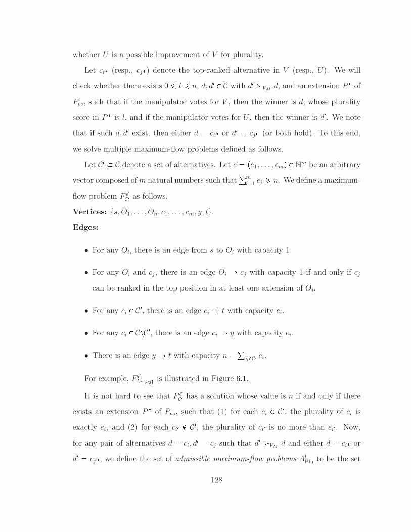
whether U is a possible improvement of V for plurality.
Let ci (resp., cj) denote the top-ranked alternative in V (resp., U). We will
check whether there exists 0 ¤ l ¤ n, d, d1 P C with d1 ¡VMd, and an extension P of
Ppo, such that if the manipulator votes for V , then the winner is d, whose plurality
score in P is l, and if the manipulator votes for U , then the winner is d1. We note
that if such d, d1 exist, then either d ci or d1 cj (or both hold). To this end,
we solve multiple maximum-flow problems defined as follows.
Let C1 C denote a set of alternatives. Let ~e pe1, . . . , emq P Nm be an arbitrary
vector composed of m natural numbers such that°m
i1 ei ¥ n. We define a maximum-
flow problem F ~eC1 as follows.
Vertices: ts, O1, . . . , On, c1, . . . , cm, y, tu.Edges:
• For any Oi, there is an edge from s to Oi with capacity 1.
• For any Oi and cj, there is an edge Oi Ñ cj with capacity 1 if and only if cj
can be ranked in the top position in at least one extension of Oi.
• For any ci P C1, there is an edge ci Ñ t with capacity ei.
• For any ci P CzC1, there is an edge ci Ñ y with capacity ei.
• There is an edge y Ñ t with capacity n °ciPC1 ei.
For example, F ~etc1,c2u is illustrated in Figure 6.1.
It is not hard to see that F ~eC1 has a solution whose value is n if and only if there
exists an extension P of Ppo, such that (1) for each ci P C1, the plurality of ci is
exactly ei, and (2) for each ci1 R C1, the plurality of ci1 is no more than ei1 . Now,
for any pair of alternatives d ci, d1 cj such that d1 ¡VM
d and either d ci or
d1 cj, we define the set of admissible maximum-flow problems AlPlu to be the set
128

s
O1
On
c3
c1
cm
t
c2
y
1
1
1
1
1
1
1
e1
e2
e3
em
n − e1 − e2
...
...
Figure 6.1: F ~etc1,c2u.of maximum flow problems F ~e
ci,cjwhere ei l, and if F ~e
ci,cjhas a solution, then the
manipulator can improve the winner by voting for U . More precisely, we define AlPlu
as follows.
• If i i and j j, then let ei l, ej l 1 δpcj, ciq, and ej minpl 1 δpj, iq, ej 1 δpj, jqq. For any ci1 P Cztci, cj, cju, we let ei1 minpl 1 δpi1, iq, ej δpi1, jqq. Let Al
Plu tF ~etci,cjuu.• If i i and j j, then let ei l, ej l δpcj , ciq, and ei minpl
1 δpi, iq, ej 1 δpi, jqq. For any ci1 P Cztci, cj, ciu, we let ei1 minpl δpi1, iq, ej 1 δpi1, jqq. Let Al
Plu tF ~etci,cjuu.• If i i and j j, then we define Al
Plu as follows.
– Let ei l, ej l 1 2δpcj, ciq. For any ci1 P Cztci, cju, we let ei1 minpl 1 δpi1, iq, ej 1 δpi1, jqq.
– Let e1i e1j l. For any ci1 P Cztci, cju, we let e1i1 minpl1δpi1, iq, ej1 δpi1, jqq. Let ~e1 pe11, . . . , e1mq.
– Let AlPlu tF ~etci,cju, F ~e1tci,cjuu.
Algorithm 4 solves all maximum-flow problems in AlPlu to check whether U is a
possible improvement of V .
129
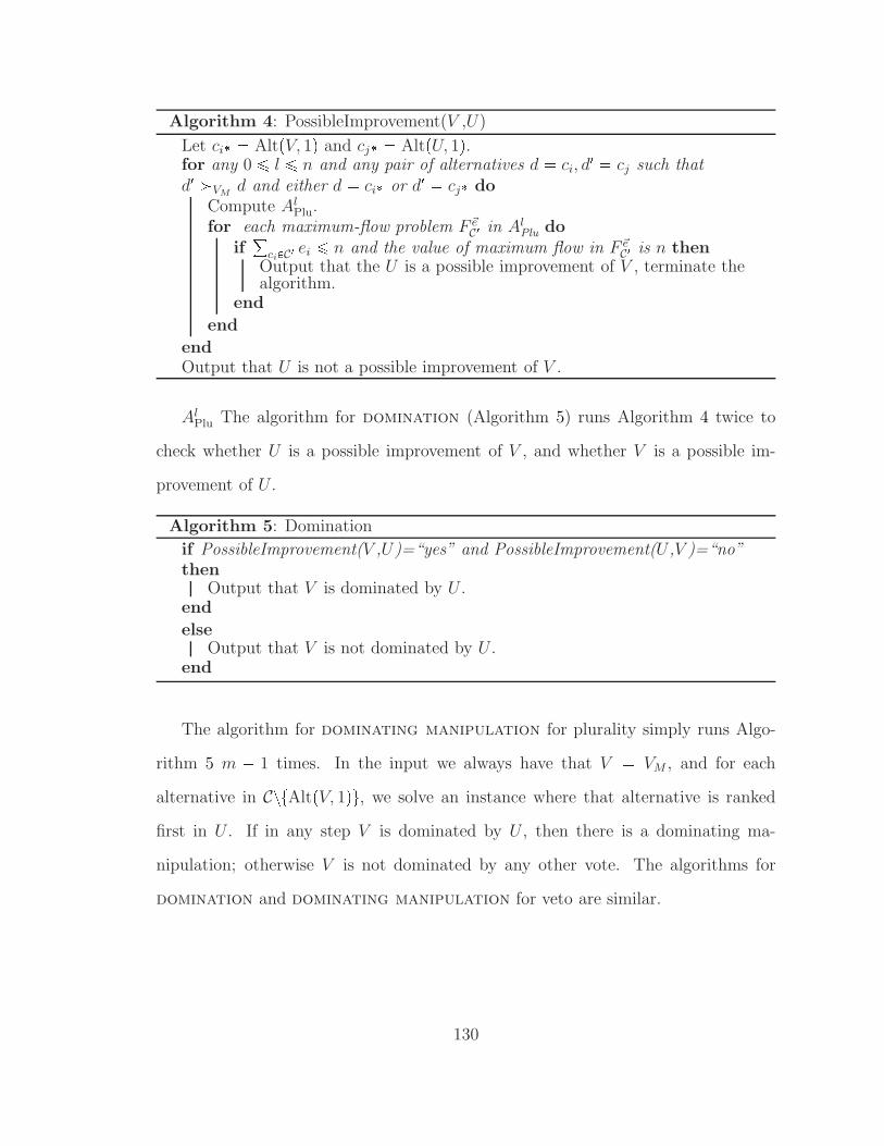
Algorithm 4: PossibleImprovement(V ,U)
Let ci AltpV, 1q and cj AltpU, 1q.for any 0 ¤ l ¤ n and any pair of alternatives d ci, d
1 cj such thatd1 ¡VM
d and either d ci or d1 cj doCompute Al
Plu.for each maximum-flow problem F ~e
C1 in AlPlu
doif°
ciPC1 ei ¤ n and the value of maximum flow in F ~eC1 is n then
Output that the U is a possible improvement of V , terminate thealgorithm.
end
end
endOutput that U is not a possible improvement of V .
AlPlu The algorithm for domination (Algorithm 5) runs Algorithm 4 twice to
check whether U is a possible improvement of V , and whether V is a possible im-
provement of U .
Algorithm 5: Domination
if PossibleImprovement(V ,U)=“yes” and PossibleImprovement(U ,V )=“no”then
Output that V is dominated by U .end
elseOutput that V is not dominated by U .
end
The algorithm for dominating manipulation for plurality simply runs Algo-
rithm 5 m 1 times. In the input we always have that V VM , and for each
alternative in CztAltpV, 1qu, we solve an instance where that alternative is ranked
first in U . If in any step V is dominated by U , then there is a dominating ma-
nipulation; otherwise V is not dominated by any other vote. The algorithms for
domination and dominating manipulation for veto are similar.
130

6.4 Summary
We have shown in this chapter that for many common voting rules, restricting the
manipulator’s information about the other voters’ votes is an effective way to make
dominating manipulation computationally hard, or even impossible. Analysis of
manipulation with partial information provides insight into what needs to be kept
confidential in an election. For instance, in a plurality or veto election, revealing
(perhaps unintentionally) part of the preferences of non-manipulators may open the
door to strategic voting.
In Chapter 4, 5, and 6 we have seen some recent work and discussions on us-
ing computational complexity as a barrier against manipulation. However, a more
important question that should be asked is: Why should we even try to prevent ma-
nipulation and other types of strategic behavior? In the next chapter, we will show
that indeed, the strategic behavior of the voters can lead to extremely undesirable
outcomes, in a type of voting games which we call Stackelberg voting games.
131
7
Stackelberg Voting Games
Using computational complexity to protect elections from manipulation, bribery,
control, and other types of strategic behavior is one of the major topics of Compu-
tational Social Choice. This raises the following fundamental question: Why should
we prevent voters’ strategic behavior? Of course we may answer this question by
arguing that people should be sincere in voting due to ethical, sociological, political,
or even divine reasons. However, after all, the most important objective of voting
is to select a “good” alternative, especially in multi-agent systems. Therefore, we
would prefer to give an answer that is similar to the following: we want to prevent
voters’ strategic behavior because it might lead to undesirable outcomes.
Showing evidence for this answer in the voting setting is not as simple as it may
seem to be. One approach is to consider the game where all voters vote at the
same time, and study the equilibria of this simultaneous-move voting game. Un-
fortunately, even in a complete-information setting where all voters’ preferences are
common knowledge, this leads to an extremely large number of equilibria, many of
them bizarre. For example, as we have seen in an example in Section 3.2, in a plural-
ity election with the lexicographic tie-breaking mechanism, it may be the case that
132

all voters’ true preferences are Obama¡Clinton¡McCain. Nevertheless, the profile
where all three voters vote for McCain¡Clinton¡Obama is a Nash equilibrium. This
equilibrium is quite robust, because voting for Obama is a waste, given that nobody
else is expected to vote for Obama and some votes went to Clinton. There has
been some work exploring different solution concepts in simultaneous-move voting
games—e.g., Farquharson (1969) and Moulin (1979)—but in some sense, the equi-
librium selection issue in the above example is inherent in settings where voters vote
simultaneously.
In many practical situations, the voters vote one after another, and the later vot-
ers know the votes cast by the earlier voters. For example, consider online systems
that allow users to rate movies or other products. We consider the setting where the
voters vote one after another in this chapter to overcome the equilibrium selection
problem. We assume that voters’ preferences over the alternatives are strict; we also
make a complete-information assumption that the voters’ preferences are common
knowledge (among the voters themselves, though not necessarily to the election or-
ganizer).1 This results in an extensive-form game of perfect information that can be
solved by backward induction. In sharp contrast to the simultaneous-move setting,
this results in a unique outcome (winning alternative). We refer to this game as a
Stackelberg voting game.
Our main theoretical results will be shown in Section 7.2. As a corollary to our
main theorem, which is quite technical but very general, we will show that for any
voting rule r that satisfies the majority criterion (see Section 2.2 for the definition),
no matter how many voters there are, there always exists a profile such that the
backward-induction winner (i.e., the unique winner in all SPNE) of the Stackelberg
1 While this is clearly a simplifying assumption, it approximates the truth in many settings, andwith this assumption we do not need to specify prior distributions over preferences. Also, naturally,our negative results still apply to more general models, including models allowing for incompleteinformation, so long as the complete-information setting is a special case.
133

voting game that uses r is ranked within the bottom two positions in all voters’ true
preferences, with only two exceptions. This result is quite negative, because it says
that if we allow voters to vote strategically, then sometimes the outcome is almost
the worst outcome for all but two voters. Therefore, to some extent we are showing
an ordinal price-of-anarchy (PoA) (Koutsoupias and Papadimitriou, 1999). The PoA
is the ratio of the optimal social welfare over the worst social welfare in equilibrium
outcomes. In fact, in the settings where social welfare is not well-defined, it is even
not clear how the PoA should be defined. Fortunately, the paradoxes we will show
are clearly very negative results.
Similar to the “worst case vs. typical case” debate about the results on hardness
of manipulation, here again we can ask how often the paradoxes happen. To answer
this question, we will pursue an empirical approach in Section 7.4. We will use the
techniques developed in Section 7.3 to run simulations to compare the backward-
induction winner to a benchmark outcome—namely, the alternative that would win
if all voters voted truthfully. Our experimental results show that, surprisingly, more
voters prefer the backward-induction outcome over the truthful outcome on aver-
age. Therefore, it seems that on average the backward-induction outcome is not too
undesirable.
The idea of modeling a voting process in which voters vote one after another as
an extensive-form game is not new. Sloth (1993) studied elections with two alterna-
tives, as well as settings with more alternatives where a pairwise decision between
two options is made at every stage. She relates the outcomes of this process to the
multistage sophisticated outcomes of the game (McKelvey and Niemi, 1978; Moulin,
1979). In the extensive-form games studied by Dekel and Piccione (2000), multi-
ple voters can vote simultaneously in each stage. They compare the equilibrium
outcomes of these games to the outcomes of the symmetric equilibria of their simul-
taneous counterparts. Battaglini (2005) studies how these results are affected by the
134

possibility of abstention and a small cost of voting.
Our approach is significantly different from the previous approaches in several
aspects. First, the prior work focuses mostly on the case of two alternatives or, in
the case of multiple alternatives, on particular voting procedures; in contrast, we
consider general (anonymous) voting rules with any number of alternatives, and cor-
respondingly derive very general paradoxes. Second, we show some paradoxes to
illustrate that the strategic behavior of the voters sometimes leads to very undesir-
able outcomes. Third, we also study how the backward-induction outcome can be
efficiently computed, and we use these algorithmic insights in simulations to evaluate
the quality of the Stackelberg voting game’s outcome “on average.”
Desmedt and Elkind (2010) simultaneously and independently studied a similar
setting in which voters vote sequentially under the plurality rule, and showed several
different types of paradoxes. In their model, voters are allowed to abstain, and
voting comes at a small cost. They assume random tie-breaking and therefore need
to consider expected utilities, while in our model studied in this chapter, voters’
preferences are ordinal.
7.1 Stackelberg Voting Game
We now consider the strategic Stackelberg voting game. We use a complete-information
assumption: all the voters’ preferences are common knowledge. Given this assump-
tion, for any voting rule r, the process where voters vote in sequence can be modeled
as an extensive-form game of perfect information. In Section 3.2 we gave the formal
definition of simultaneous-move voting games, and mentioned that extensive-form
voting games can be defined similarly. Here I will be more specific. The game has
n stages. In stage j (j ¤ n), voter j chooses an action from LpCq. Each leaf of the
tree is associated with an outcome, which is the winner for the profile consisting of
the votes that were cast to reach this leaf.
135

Because the voters’ preferences are linear orders (which implies that there are
no ties), we can solve the game by backward induction, which results in a unique
outcome. We note that this requires only ordinal preferences, that is, we do not
need to define utilities. The backward-induction process works as follows. First, for
any subprofile of votes by the voters 1 through n 1 (that is, any node that is the
parent of leaves), there will be a nonempty subset of alternatives that n can make
win by casting some vote. She will pick her most preferred one. Now, because we can
predict what voter n will do, we take voter pn1q’s perspective: for any subprofile of
votes by the voters 1 through n 2, there will be a nonempty subset of alternatives
that voter n 1 can make win by casting some vote (taking into account how voter
n will act). She will pick her most preferred one; etc. We continue this process all
the way to the root of the tree; the outcome there is called the backward-induction
outcome.
As noted above, only the ordinal preferences of the voters matter; that is, a voter’s
preferences correspond to a member of LpCq. While votes and preferences both lie in
the same set LpCq, we must be careful to distinguish between them, because in this
context, a voter will sometimes cast a vote that is different from her true preferences.
Nevertheless, we can use P P Fn to denote a profile of preferences, as well as a profile
of votes. For a given voting rule r, let rpP q be the outcome if the votes are P ; let
SGrpP q be the backward-induction outcome if the true preferences are P .2
7.2 Paradoxes
In this section, we investigate whether the strategic behavior described above will
lead to undesirable outcomes. It turns out that it can. Our main theorem is a
2 Of course, because it is a function from profiles of linear orders to alternatives, SGr can alsobe interpreted as a voting rule, though there is a significant risk of confusion in doing so. We notethat even if r is anonymous, SGr (as a voting rule) is not necessarily anonymous (the order of thevoters matters).
136

general result that applies to many common voting rules. We will show that, for
such a rule, there exists a profile that has two types of paradox associated with it in
the backward-induction outcome: first, the winner loses all but one of its pairwise
elections; second, the winner is ranked somewhere in the bottom two positions in
almost every voter’s true preferences. For the second type of paradox, we will show
that the number of exceptions (voters who rank the winner higher) is closely related
to a parameter called the domination index. The domination index of a voting rule
r that satisfies non-imposition is the smallest number q such that any coalition oftn2u q voters can make any given alternative win (no matter how the remaining
voters vote) under r. We note that the domination index is always well defined for
any rule that satisfies non-imposition, and is at least 1.
Definition 7.2.1. For any voting rule r that satisfies non-imposition, and any n PN, we let the domination index DIrpnq be the smallest number q such that for any
alternative c, and for any subset of tn2u q voters, there exists a profile P for these
voters, such that for any profile P 1 for the remaining voters, rpP Y P 1q c.
The domination index DIr is closely related to the anonymous veto function
VFr : t1, . . . , nu Ñ t0, . . . , mu (Definition 10.4 in Moulin (1991)), defined as follows.
VFrpiq is the largest number j ¤ m 1 such that any coalition of i voters can veto
any subset (that is, make sure that none of the alternatives in the set is the winner)
of no more than j alternatives. We note that the domination index DIrpnq for a
voting rule r is the smallest number q such that VFrptn2u qq m 1 (that is,
any coalition of size tn2u q can veto any set of m 1 alternatives).
The next proposition gives bounds on the domination index for some common
voting rules.
Proposition 7.2.2. For any positional scoring rule r, DIr ¤ tn2utnmu. DIrpnq 1 for any voting rule r that satisfies the majority criterion (Section 2.2), including
137

any rule that satisfies the Condorcet criterion (Section 2.2), plurality, plurality with
runoff, Bucklin, and STV.
The next lemma provides a sufficient condition for an alternative not to be the
backward-induction winner. It says that if there is a coalition of size k ¥ tn2u DIrpnq who all prefer c to d, and another condition holds, then d cannot win.3 For any
alternative c P C and any V P LpCq, we let Uppc, V q denote the set of all alternatives
that are ranked higher than c in V .
Lemma 7.2.3. Let P be a profile. An alternative d is not the winner SGrpP q if there
exists another alternative c and a sub-profile Pk pVi1 , . . . , Vikq of P that satisfies
the following conditions: 1. k ¥ tn2u DIrpnq, 2. c ¡ d in each vote in Pk, 3. for
any 1 ¤ j1 j2 ¤ k, Uppc, Vij1q Uppc, Vij2
q.Proof. Let Dk ti1, . . . , iku. Since k ¥ tn2u DIrpnq, this coalition of voters can
guarantee that any given alternative be the winner under r, if they work together.
Let P k pV i1, . . . , V
ikq be a profile that can guarantee that c be the winner under r.
That is, for any profile P 1 for the other voters (t1, . . . , nuzDk), we have rpP k , P 1q c.
For any j ¤ k, we let D1ij t1, . . . , ijuzDk—that is, the first ij voters, except those
in the coalition Dk. For any j ¤ k, we let P j pV i1, . . . , V
ijq. That is, P j consists
of the first j votes in P k . For any i ¤ n 1 and any pair of profiles P1 (consisting of
i votes) and P2 (consisting of n i votes), we let SGrpP2 : P1q denote the backward-
induction winner of the subgame of the Stackelberg voting game in which voters 1
through i have already cast their votes P1, and the true preferences of voters i 1
through n are as in P2. We prove the following claim by induction.
3 This may seem trivial because the coalition can guarantee that c wins if they work together.However, we have to keep in mind that the members of the coalition each pursue their own interest.For example, it may be the case that whenever the second-to-last voter in the coalition votes in away that enables the last voter in the coalition to make c the winner, it also enables this last voterto make e the winner, which this last voter prefers—but the second-to-last voter actually prefersd to e, and therefore votes to make d win instead. We need the extra condition to rule out suchexamples.
138

Claim 7.2.1. For any j ¤ k and any profile P 1ij for the voters in D1ij,
SGrppVij , Vij1, . . . , Vnq : P 1ij , P j1q ©Vijc
Claim 7.2.1 states that for any j ¤ k, if voters i1, . . . , ij1 have already voted
as in P j , and voter ij will vote next, then the backward-induction outcome of the
corresponding subgame must be (weakly) preferred to c by voter ij .
Proof of Claim 7.2.1: The proof is by (reverse) induction on j. First, we consider
the base case where j k. If voter ik casts V ik
, then the winner is c, because the
subprofile P k will guarantee that c wins. Voter ik will only vote differently if it
results in at least as good an outcome for her as c. Therefore, the claim holds for
j k.
Now, suppose that for some j1, the claim holds for j1 ¤ j ¤ k. We will now show
that it also holds for j j1 1. Let c1 be the backward-induction outcome when
voter ij11 submits V ij11
. By the induction hypothesis, we have that c1 ©Vij1 c. That
is, voter ij1 (weakly) prefers c1 to c. We recall that Uppc, Vij11q Uppc, Vij1 q, which
means that c1 is also (weakly) preferred to c by voter ij11. This means that voter
ij11 can guarantee that the outcome be at least as good as c for her. She will only
vote differently from V ij11
if it results in at least as good an outcome for her as c1(which is at least as good as c already). Therefore, the claim also holds for j1 1,
and Claim 7.2.1 follows by induction. lLetting j 1 in Claim 7.2.1, we have that SGrpP q ©Vi1
c. Therefore, d SGrpP q(because c ¡Vi1
d). This completes the proof of Lemma 7.2.3.
We are now ready to present our main theorem. We note that this theorem does
not depend on the tie-breaking mechanism used in the rule.
Theorem 7.2.4. For any voting rule r that satisfies non-imposition, and any n P N,
there exists a profile P such that SGrpP q is ranked somewhere in the bottom two
139
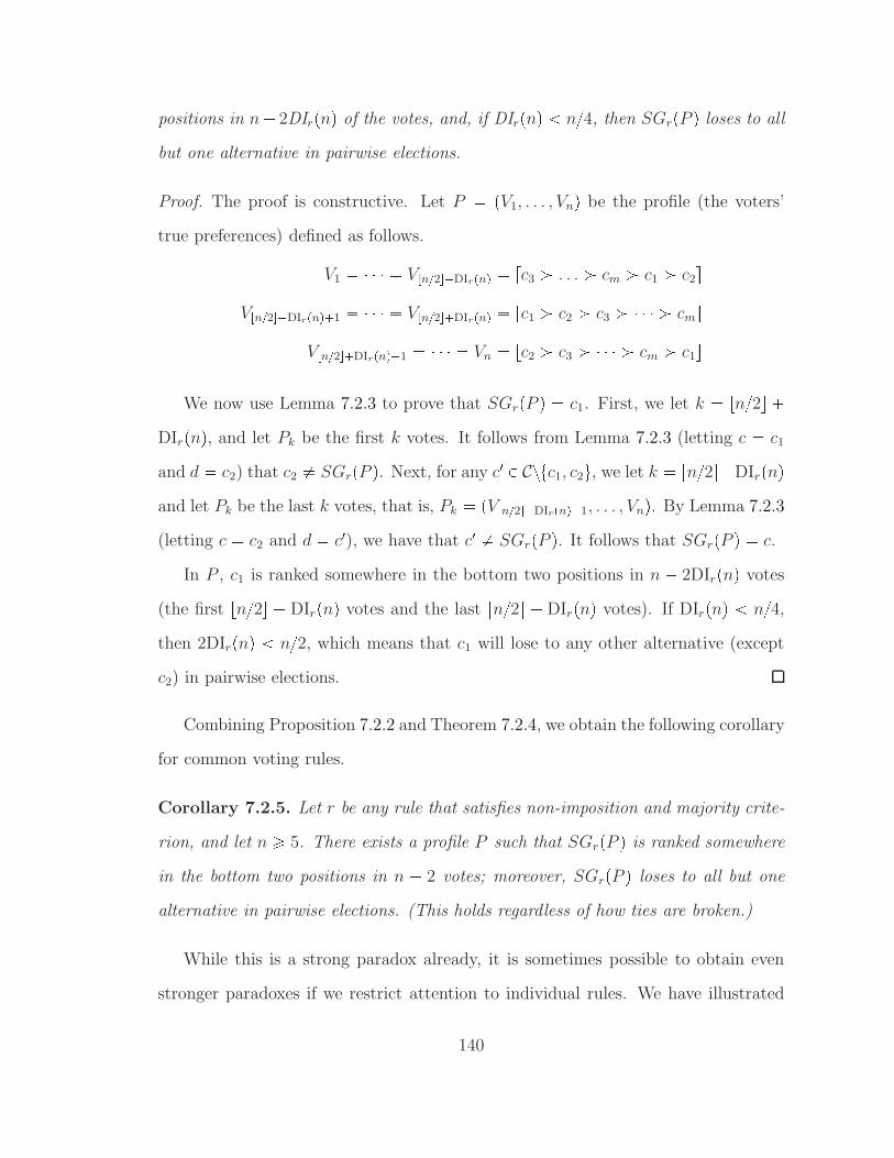
positions in n 2DIrpnq of the votes, and, if DIrpnq n4, then SGrpP q loses to all
but one alternative in pairwise elections.
Proof. The proof is constructive. Let P pV1, . . . , Vnq be the profile (the voters’
true preferences) defined as follows.
V1 Vtn2uDIrpnq rc3 ¡ . . . ¡ cm ¡ c1 ¡ c2sVtn2uDIrpnq1 Vtn2uDIrpnq rc1 ¡ c2 ¡ c3 ¡ ¡ cms
Vtn2uDIrpnq1 Vn rc2 ¡ c3 ¡ ¡ cm ¡ c1sWe now use Lemma 7.2.3 to prove that SGrpP q c1. First, we let k tn2u
DIrpnq, and let Pk be the first k votes. It follows from Lemma 7.2.3 (letting c c1
and d c2) that c2 SGrpP q. Next, for any c1 P Cztc1, c2u, we let k rn2sDIrpnqand let Pk be the last k votes, that is, Pk pVtn2uDIrpnq1, . . . , Vnq. By Lemma 7.2.3
(letting c c2 and d c1), we have that c1 SGrpP q. It follows that SGrpP q c.
In P , c1 is ranked somewhere in the bottom two positions in n 2DIrpnq votes
(the first tn2u DIrpnq votes and the last rn2s DIrpnq votes). If DIrpnq n4,
then 2DIrpnq n2, which means that c1 will lose to any other alternative (except
c2) in pairwise elections.
Combining Proposition 7.2.2 and Theorem 7.2.4, we obtain the following corollary
for common voting rules.
Corollary 7.2.5. Let r be any rule that satisfies non-imposition and majority crite-
rion, and let n ¥ 5. There exists a profile P such that SGrpP q is ranked somewhere
in the bottom two positions in n 2 votes; moreover, SGrpP q loses to all but one
alternative in pairwise elections. (This holds regardless of how ties are broken.)
While this is a strong paradox already, it is sometimes possible to obtain even
stronger paradoxes if we restrict attention to individual rules. We have illustrated
140

this on some voting rules including plurality, which can be found in Xia and Conitzer
(2010b).
7.3 Computing the Backward-Induction Outcome
We have shown in the last section that the backward-induction solution to the Stack-
elberg voting game is socially undesirable for some profiles. We may ask ourselves
whether such profiles are common, or just isolated instances that are not very likely
to happen in practice. For this purpose, we would like to compare the backward-
induction winner to the truthful winner by running simulations. For this purpose,
we should be able to compute the backward-induction winners reasonably fast. How-
ever, even if the outcome of the rule r is easy to compute, it does not follow that
the outcome of SGr is easy to compute. The straightforward backward-induction
process described above is very inefficient, because the game tree has pm!qn leaves.
In this section, we first propose a general dynamic-programming algorithm to
compute SGrpP q, for any anonymous voting rule r. Then, we show how to use com-
pilation functions (Chevaleyre et al., 2009) (see also Section 1.6) to further reduce the
time/space-complexity of the dynamic-programming algorithm. These techniques
are crucial for obtaining our later experimental results.
The dynamic-programming algorithm still solves the game tree in a bottom-up
fashion, but does not need to consider all the different profiles separately. Because
r is anonymous, at any stage j of the game, the state (the profile of votes 1 through
j 1) can be summarized by a vector composed of m! natural numbers, one for each
linear order: each number in the vector represents the number of times that the
corresponding linear order appears in the pj1q-profile. Formally, for any j ¤ n, we
let the set of these vectors (states) be Sj tps1, . . . , sm!q P N¥0m! :
°m!i1 si j 1u.
For any anonymous voting rule r and any ~s P Sn1, let rp~sq be the winner for any
profile that corresponds to ~s (because r is anonymous, the winner only depends on
141

the vector ~s). More generally, for arbitrary Sj, the algorithm computes a labeling
function g that maps each state ~s P Sj to the alternative representing the backward-
induction outcome of the subgame whose root corresponds to ~s.
Algorithm 7.3.1.
Input. P pV1, . . . , Vnq and an anonymous voting rule r.
Output. SGrpP q.1. For j from n 1 to 1, do Step 2.
2. For any state ~s P Sj , do
2.1 If j n 1, then let gp~sq rp~sq.2.2 If j n1, then let ~e P arg min~ePE rankpVj , gp~s~eqqq, where E consists of
all vectors that are composed of m!1 zeroes and only one 1, and rankpVj, gp~s~eqq is the position of gp~s ~eq in Vj. (Thus, e corresponds to an optimal vote
for j.) Then, let gp~sq gp~s ~eq.3. Output gpp0, . . . , 0qq.Analysis. For any j ¤ n, |Sj| jm!2
m!1
(this is a basic combinatorial result, see
e.g. Bender and Williamson (2006)). To analyze the runtime of the algorithm, we
note that the total number of states considered is°n1
j1
jm!2m!1
, which is Oppn
1qm!1q; in each state, we need to consider m! vectors ~e, resulting in a total bound
of Opm!pn 1qm!1q. To analyze the space requirements of the algorithm, we note
that we only need to keep the last stage j 1 and the current stage j in memory,
so that the maximum number of states in memory is
nm!1m!1
nm!2m!1
, which is
Oppn 1qm!q. Therefore, when m is bounded above by a constant, Algorithm 7.3.1
runs in polynomial time (using polynomial space).
However, when there is no upper bound on m, Algorithm 7.3.1 runs in exponential
time and uses exponential space. We conjecture that for many common voting rules
142

(e.g., plurality), computing SGr is PSPACE-hard, but we have not managed to
obtain any such result yet.4
Compilation. In the step corresponding to stage j in Algorithm 7.3.1, a very large
set Sj is used to keep track of all possible m!-dimensional vectors whose entries sum
to exactly j 1, representing the possible states. While it may be necessary to have
this many states for anonymous rules in general, it turns out that for specific rules
like plurality or veto, we need far fewer states to represent the profiles, because many
of the states in Algorithm 7.3.1 will be equivalent for the specific rule. For example,
if we have so far received only a single vote a ¡ b ¡ c, this in general is not equivalent
to having received only a single vote a ¡ c ¡ b. However, if the rule is plurality,
these states are equivalent.
Pursuing this idea, for any anonymous voting rule r, we can ask the following
questions. (1) What is the smallest set of states needed for stage j? (2) How can we
incorporate smaller sets of states into Algorithm 7.3.1?
The answer to question (1) corresponds to the compilation complexity of r, a
concept introduced by Chevaleyre et al. (2009). For any k, u P N with k u n,
the compilation complexity Cm,k,uprq is defined to be the smallest number of bits
needed to represent all “effectively different” k-profiles, when there are u remaining
votes and the winner is chosen by using r. (Two k-profiles are “effectively the same”
if, for any profile of u votes that we may add to them, they result in the same
outcome.) It follows that, if we tailor Algorithm 7.3.1 to a specific rule r, the size
of the smallest possible set of states for stage j is between 2Cm,j1,nj1prq1 and
2Cm,j1,nj1prq. Chevaleyre et al. (2009) also studied the compilation complexity for
some common voting rules.
Now we turn to address question (2). Suppose that we have already determined
4 We have obtained a PSPACE-hardness result for a not-so-common rule with a different typeof voter preferences, which thus falls somewhat outside of the setting described so far. We omit itdue to the space constraint.
143

that we can use a smaller set of states. In order to modify the dynamic-programming
algorithm to use this smaller set of states, for step (2.2) we must have a function that
takes a state in Sj and a vote V as inputs, and outputs a state in Sj1; moreover, this
function must be easy to compute. Fortunately, the compilation functions designed
for some common voting rules in Chevaleyre et al. (2009) and Xia and Conitzer
(2010a), which map each profile to a string (state), can serve as such functions.
For example, the compilation function for plurality simply counts how often each
alternative has been ranked first, and this is easy to update. More generally, we can
modify Algorithm 7.3.1 for any specific rule r as follows. Let f rm,k,u be a compilation
function for r. For any j ¤ n, we let Sj f rm,k,upFj1q, that is, the set of all
“compressed” pj 1q-profiles. Then, in step (2.2), for each given state ~s P Sj and
each5 given vote V P LpCq, the next state (which lies in Sj1) is computed by applying
the compilation function f rm,k,u to the combination of ~s and V . Among these resulting
states, we again find voter j’s most-preferred outcome.
Illustration. Let us illustrate how the use of compilation functions helps reduce
the time and space requirements of Algorithm 7.3.1 for the nomination rule, which
selects the alternative that is ranked in the first position in at least one vote, where
ties are broken in the order c1 ¡ ¡ cm. In this case, for any j ¤ n, let Sj C, and
let fNom be the following compilation function. For any profile P , let fNompP q be
the first alternative (according to the order c1 ¡ ¡ cm) that has been nominated
(is ranked first in some vote in P ). For any profile P and any vote V , fNompP YtV uqcan be easily computed from fNompP q and V , by determining which of fNompP q and
the alternative ranked in the top position in V is earlier in the order. (As in the
case of plurality, we do not need to consider every vote V : we only need to consider
which alternative is ranked first.) Because |Sj| m for all j in this case, it follows
5 For some rules, we do not need to consider every vote: for example, under plurality, we do notneed to consider both a ¡ b ¡ c and a ¡ c ¡ b.
144

that Algorithm 7.3.1 (using fNom) runs in polynomial time for the nomination rule.
Proposition 7.3.1. SGNom can be computed in polynomial time (and space) by
Algorithm 7.3.1 (using fNom).
For other, more common voting rules, the runtime of the dynamic-programming
algorithm is also significantly reduced by using compilation functions, though it
remains exponential. For example, for plurality and veto, the time/space complexity
of our approach is Opnmq, which allows us to conduct the simulation experiments in
the next section much more efficiently.
7.4 Experimental Results
Using the algorithmic techniques developed in the last section, we are able to run
simulations to compare the backward-induction winner SGrpP q to a benchmark
outcome—namely, the alternative rpP q that would win under r if all voters vote
truthfully. This may seem like a difficult benchmark to achieve, because often
strategic behavior comes at a cost (cf. price of anarchy, first-best vs. second-best
in mechanism design, etc.) Nevertheless, in the experiments that we describe in this
section, it turns out that in randomly chosen profiles, in fact, slightly more voters
prefer the backward-induction outcome SGrpP q to the truthful outcome rpP q than
vice versa!
The setup of our experiment is as follows. We study the plurality and veto rules
(these are the easiest to scale to large numbers of voters, because they have low
compilation complexity).6
For any m, n, and r P tPlurality, Vetou, our experiment has 25,000 iterations. In
each iteration, we perform the following three steps.
6 We also investigated other rules. It appears that they may lead to similar results, though itis difficult to say this with high confidence because we can only solve for the backward-inductionoutcome for small numbers of voters.
145

1. In iteration j, an n-profile Pj is chosen uniformly at random from Fn.
2. We calculate SGrpPjq using Algorithm 7.3.1 (with a compilation function to
reduce time/space-complexity), and we calculate rpPjq.3. We then count the number of voters in this profile P that prefer SGrpP q to
rpP q (according to their true preferences in P ), denoted by n1, and vice versa,
denoted by n2. If SGrpP q rpP q, then n1 n2 0.
For each m, n, r, we calculate the total percentage (across all 25,000 iterations)
of voters that prefer the backward-induction winner for their profile to the winner
under truthful voting for their profile, that is, p1 °25000j1 n
j1p25000nq. We also
compute p2 °25000j1 n
j2p25000nq. We note that it is not necessarily the case that
p1 p2 1, because if SGrpP q rpP q, then n1 n2 0. Let p3 1 p1 p2 be
the percentage of profiles for which the backward-induction (SGr) winner coincides
with the truthful (r) winner. We are primarily interested in p1 p2.
The results are summarized in Figure 7.1.
146

5 10 15 202−2
0
2
4
6
8
10
12m=3
m=4
m=5
m=6
m=7
5 10 15 20240
50
60
70
80
90
(a) (b)
5 10 15 2020
5
10
15
20
25
30m=3
m=4
m=5
m=6
m=7
5 10 15 20240
50
60
70
80
90
(c) (d)
Figure 7.1: Simulation results for plurality and veto
In Figure 7.1, the x-axis gives the number of voters (n); the y-axis gives the
percentage of voters. In each case we consider various numbers of alternatives (m).
(a) The percentage of voters who prefer the SGr winner to the r winner minus the
other way around, under plurality. (b) The percentage of profiles for which the SGr
winner and the r winner are the same, under plurality. (c) The percentage of voters
who prefer the SGr winner to the r winner minus the other way around, under veto.
(d) The percentage of profiles for which the SGr winner and the truthful r winner
are the same, under veto. Please note the different scales on the y-axis for (a) and
147

(c).
First, from (a) and (c) it can be observed that for plurality and veto, perhaps
surprisingly, on average, more voters prefer the backward-induction winner to the
winner under truthful voting than vice versa. Generally, the difference becomes
smaller when n increases; the difference is larger when m is larger; and the percentage
seems to converge to some limit as n Ñ 8. Second, from (b) and (d) it can be
observed that the percentage of profiles for which the two winners coincide is smaller
for larger values of m; the percentage is decreasing in the number of voters n for
plurality, but increasing for veto.
7.5 Summary
In this chapter we studied the voting game where voters cast votes one after an-
other and the later voters can observe all previous voters’ votes. We proved some
paradoxes, which state that sometimes the strategic behavior of the voters can be
harmful in Stackelberg voting games. To some extent, these paradoxes justify the
line of research in which people seek to use computational complexity to prevent
strategic behavior. We also developed algorithmic techniques to run simulations.
Our simulation results show that, surprisingly, the strategic behavior of the voters
does not seem as harmful as we might have expected.
148
8
Introduction to Combinatorial Voting
We recall from Section 2.3 that one major direction in Computational Social Choice
is to investigate the computational complexity of winner determination for some
common voting rules, and then design heuristic, fixed-parameter tractable, or ap-
proximation algorithms for voting rules for which the winner is hard to compute.
In those situations, the computational complexity mainly comes from the choice of
voting rule.
However, in many real life group decision making problems, the computational
complexity comes from the extremely large number of alternatives. In such cases
it may take an unbearably long time to compute the winner even for simple voting
methods such as Borda. Perhaps the most natural and prominent voting setting
in real-life with an extremely large number of alternatives is combinatorial voting,
a.k.a. voting in multi-issue domains. In combinatorial voting, the set of alternatives
has a combinatorial (namely, multi-issue) structure. That is, there are multiple issues
(or attributes, or characteristics) and each alternative can be uniquely characterized
by a vector of the values these issues take. For example, consider a situation where
the inhabitants of a county vote to determine a government plan. The plan is com-
149

posed of multiple sub-plans for several interrelated issues, such as transportation,
environment, and health (Brams et al., 1998). Another example is voting by com-
mittees, in which the voters select a subset of objects (Barbera et al., 1991), where
each object can be seen as a binary issue. In such situations, a voters’ preferences
over one issue may well depend on the values of other issues. For example, a voter
may prefer creating a natural reserve if a highway is built, but if the highway is not
built, she may prefer not creating a reserve.
In the remainder of this dissertation (Chapter 8–12), we will focus on the design
and analysis of voting rules when the set of alternatives has a multi-issue structure. In
this chapter, we give the formal definitions and notation that will be used throughout
these chapters.
Definition 8.0.1 (Combinatorial voting). Let I tX1, . . . , Xpu denote a set of p ¥2 issues, where for each i ¤ p, Xi takes a value in a local domain Di, where |Di| ¥ 2.1
Combinatorial voting refers to the voting setting where the set of alternatives is
X D1 Dp. X is called a multi-issue domain or combinatorial domain.
Example 8.0.2. A group of people must make a joint decision on the menu for
dinner (the caterer can only serve a single menu to everyone). The menu is composed
of two issues: the main course (M) and the wine (W). There are three choices for
the main course: beef (b), fish (f), or salad (s). The wine can be either red wine (r),
white wine (w), or pink wine (p). The set of alternatives is a multi-issue domain:
X tb, f, su tr, w, pu.We call that the set of alternatives C studied in previous chapters constitutes an
unstructured domain, because it does not need to have a multi-issue structure. In the
above definition, we use X (instead of C) to emphasize that the set of alternatives
1 This is the standard assumption for studying voting in multi-issue domains, because otherwiseeither the domain can be simplified (by removing issues that can only take one value), or it has nomulti-issue structure (when there is only one issue).
150

has a multi-issue structure. Following convention, for any i ¤ p we let Di D1 Di1 Di1 Dp.
A special case of multi-issue domains consists of the domains where all variables
are binary, that is, for all i ¤ p, Di t0i, 1iu. Such multi-issue domains are called
multi-binary-issue domains. Even in multi-binary-issue domains, the number of al-
ternatives is 2p, which is already exponentially large. Moreover, we recall that the
voting setting we defined in Chapter 2 requires a voter to submit a linear order over
the set of alternatives. This requirement causes the major problem in combinato-
rial voting, which is that it is infeasible for a voter to give a full ranking over an
exponentially large number of alternatives. Therefore, in combinatorial voting, the
voters need to use another voting language to represent their preferences, and then
we can design novel voting rules to aggregate voters’ preferences represented by such
a voting language.
An obvious solution is the following: we can simply ask voters to report only
a (small) part of their preference relation and apply a voting rule that needs this
information only. For example, we can ask the voters to report their most-preferred
alternatives, and then apply the plurality rule. The voting language used in this case
is the set of all alternatives instead of the set of all linear orders over the alternatives.
One problem with this type of solution is the following: as soon as the number of
alternative is large (2p " n), the voters are likely to be unhappy about only expressing
a small portion of their preferences. Moreover, the result of voting is likely to be
completely insignificant or even catastrophic. For instance, with 5 voters and 6
binary issues, it is very likely that all 5 voters vote for different alternatives (since
there are 26 64 alternatives), and the winner under the plurality rule might be
disliked by all but one voter. In fact, this phenomenon is a type of multiple-election
paradox, which we will discuss in more detail in the next section.
Even though the above (plurality) solution itself does not work very well, it
151

reveals the following two important high-level criteria for voting rules in multi-issue
domains.
The first criterion: The quality of the voting language, which includes compactness
and expressiveness.
The second criterion: The quality of the voting rule after the votes have been
collected. Here the quality is measured by computational efficiency, satisfia-
bility of axiomatic properties (see Section 2.2), resistance to multiple-election
paradoxes, etc.
The compactness of a voting language can be measured by the number of bits that
is used to represent a voter’s preferences. For example, Θpp 2pq bits are necessary
and sufficient to represent the voting language that consists of all linear orders over
X , because logpp2pq!q is Θpp 2pq. Measuring the expressiveness of a voting language
is more complicated. We consider the following two dimensions.
The first dimension of expressiveness: the general usability of the language.
That is, the percentage of voters who are comfortable using this language to
express their preferences. For example, if we only ask the voters to report their
top-ranked alternative, no voter will feel ill at ease to do so. However, as we
will see in the next section, voters are not always comfortable expressing their
preferences in issue-by-issue voting and sequential voting.
The second dimension of expressiveness: the informativeness of the language.
That is, how much of the voters’ preferences are expressed by the language. For
example, the top-ranked alternative only represents a tiny portion of the voter’s
preferences. The languages used in issue-by-issue voting rules and sequential
voting rules both allow voters to express much more of their preferences.
152

8.1 Multiple-Election Paradoxes
Combinatorial voting has been extensively studied by economists. Most of previous
work has focused on letting voters vote on the issues separately, in the following way.
For each issue (simultaneously, not sequentially), each voter reports her preferences
for that issue, and then, a local rule is used to select the winning value that the
issue will take. This voting process is called issue-by-issue or seat-by-seat voting.2
Recently, Ahn and Oliveros (2011) studied a Bayesian game of combinatorial voting,
and showed the existence equilibrium under some conditions. We will not discuss
the Bayesian setting in this dissertation.
Issue-by-issue voting has some drawbacks. First, a voter may feel uncomfortable
expressing her preferences over one issue independently of the values that the other
issues take. This means that, even though the voting language used in issue-by-issue
voting can express more of a voter’s preferences than the voting language that is used
in plurality, it lack usability. That is, only voters whose preferences are separable
(that is, for any issue i, regardless of the values for the other issues, the voter’s pref-
erences over issue i are always the same) are comfortable expressing their preferences
in issue-by-issue voting (Kadane, 1972; Schwartz, 1977). Second, multiple-election
paradoxes arise in issue-by-issue voting (Brams et al., 1998; Scarsini, 1998; Lacy and
Niou, 2000), which we will discuss below in more detail.
Brams et al. (1998) showed that for multi-binary-issue domains, there exists a
profile where the winner under issue-by-issue voting (where all local voting rules are
majority rules) receives zero votes (that is, it is never ranked in the top position by
any voter). Scarsini (1998) showed an even stronger paradox: there exists a profile
2 The names “issue-by-issue” and “seat-by-seat” are a little bit misleading. It may sound likethere is an ordering over issues, according to which the voters vote over issues sequentially. Eventhough the election can be organized in this sequential way, effectively these issue-wise electionsare conducted in parallel in issue-by-issue voting, because the voters do not learn the outcomes ofother issues before deciding on an issue.
153

where any alternative that is “close” to the winner in terms of Hamming distance
under issue-by-issue voting receives zero votes. These paradoxes exist even when the
voters’ preferences are separable.
We are more interested in the paradoxes demonstrated by Lacy and Niou (2000)
for issue-by-issue voting when the voters’ preferences are non-separable. Of course
in such cases the voters may feel ill at ease reporting their preferences over a single
issue without knowing the values of the other issues. In Lacy and Niou (2000), it is
assumed that voters vote according to their top-ranked alternative. That is, when
a voter is asked to report her preferences over issue Xi, she will report the value
of the Xi component in her top-ranked alternative. This behavior in some sense
corresponds to very optimistic voters, and Lacy and Niou argued that when a voter
does not know the votes of the other voters, she is likely to vote in this way. They
illustrated the paradoxes in the following example.
Example 8.1.1. Suppose there are three voters and the multi-issue domain is com-
posed of three binary issues. The top-ranked alternatives of the three voters are 110,
101, and 011, respectively; and all voters rank 111 in their bottom positions. Now,
by voting over each issue separately in parallel using the majority rule, the winner is
111, which is the least-preferred alternative for all voters.
The above example illustrates the following three types of multiple-election para-
doxes for issue-by-issue voting:
First type of paradox: the winner is a Condorcet loser (who loses to all the
other alternatives in their pairwise elections).
Second type of paradox: the winner is Pareto-dominated by another alter-
native (that is, that alternative is preferred to the winner by all voters).
154

Third type of paradox: the winner is ranked in a very low position in all
voters’ true preferences.
8.2 CP-nets
We have seen so far that none of the approaches mentioned above works well. One
common deficiency of them is that the voting languages are not expressive enough.
We have seen that the voting language used by plurality has a high usability (meaning
that all voters are comfortable using it), but it lacks informativeness (meaning that
it only represents a tiny portion of the voters’ preferences). The language used by
issue-by-issue voting is much less usable, because only voters whose preferences are
separable are comfortable with reporting their preferences in issue-by-issue voting,
and only a tiny fraction of the linear orders are separable (Hodge, 2006). But in gen-
eral it is much more informative when the voters’ preferences are separable. However,
none of these languages model the preferential dependence among the issues.
Fortunately, a new language for preference representation in multi-issue domains,
called conditional preference networks, or CP-nets, that captures the dependence
of voters’ preferences among individual issues, was recently proposed in Artificial
Intelligence (Boutilier et al., 2004). Next, we first give the formal definition of CP-
nets, then discuss how to use them as the voting language for sequential voting.
The definition of a CP-net is similar to that of a Bayesian network (Pearl, 1988).
We first give the formal definitions, and the present an example.
Definition 8.2.1. A CP-net N over X consists of two parts:
(a) A directed graph G pI, Eq.(b) A set of conditional linear preferences ¡i
~dover Di, for each setting ~d of the
parents of Xi in G. Let CPT pXiq be the set of the conditional preferences of a
voter on Di; this is called a conditional preference table (CPT).
155

A CP-net N captures dependencies across issues in the following sense. N induces
a partial preorder ¡N over the alternatives X , representing the voter’s preferences,
as follows: for any ai, bi P Di, any setting ~d of the set of parents of Xi (denoted by
ParGpXiq), and any setting ~z of IzpParGpXiq Y tXiuq, pai, ~d, ~zq ¡N pbi, ~d, ~zq if and
only if ai ¡i~dbi. In words, the preferences over issue Xi only depend on the setting
of the parents of Xi (but not on any other issues). For any 1 ¤ i ¤ p, CPTpXiqspecifies conditional preferences over Xi. Now, if we obtain an alternative ~d1 from ~d
by only changing the value of the ith issue of ~d, we can look up CPTpXiq to conclude
whether the voter prefers ~d1 to ~d, or vice versa. In general, however, from the CP-net,
we will not always be able to conclude which of two alternatives a voter prefers, if
the alternatives differ on two or more issues. This is why N usually induces a partial
preorder rather than a linear order.
When the graph of N is acyclic, ¡N is transitive and asymmetric, that is, a strict
partial order (Boutilier et al., 2004). Let O X1 ¡ ¡ Xp. We say that a CP-net
N is compatible with (or, follows) O, if the following is true: if Xi is a parent of Xj
in the graph, then this implies that i j. That is, preferences over any issue only
depend on the values of earlier issues in O. A CP-net is separable if there are no
edges in its graph, which means that there are no preferential dependencies among
issues.
Example 8.2.2. Let X be the multi-issue domain defined in Example 8.0.2. We
define a CP-net N as follows: M (the main course) is the parent of W (the wine),
and the CPTs consist of the following conditional preferences: CPT pMq tb ¡ f ¡su, CPT pWq tb : r ¡ p ¡ w, f : w ¡ p ¡ r, s : p ¡ w ¡ ru, where b : r ¡ p ¡ w
is interpreted as follows: “when M is b, then, r is the most preferred value for W,
p is the second most preferred value, and w is the least preferred value.” N and its
induced partial order ¡N are illustrated in Figure 8.1. N is compatible with M ¡W.
156
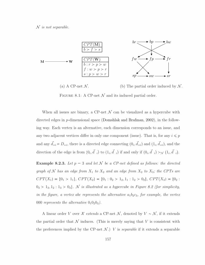
N is not separable.
M W
CPT pMqb ¡ f ¡ s
CPT pWqb : r ¡ p ¡ w
f : w ¡ p ¡ r
s : p ¡ w ¡ r
br bp bw
fw fp fr
sp sw sr
(a) A CP-net N . (b) The partial order induced by N .
Figure 8.1: A CP-net N and its induced partial order.
When all issues are binary, a CP-net N can be visualized as a hypercube with
directed edges in p-dimensional space (Domshlak and Brafman, 2002), in the follow-
ing way. Each vertex is an alternative, each dimension corresponds to an issue, and
any two adjacent vertices differ in only one component (issue). That is, for any i ¤ p
and any ~di P Di, there is a directed edge connecting p0i, ~diq and p1i, ~diq, and the
direction of the edge is from p0i, ~diq to p1i, ~diq if and only if p0i, ~diq ¡N p1i, ~diq.Example 8.2.3. Let p 3 and let N be a CP-net defined as follows: the directed
graph of N has an edge from X1 to X2 and an edge from X2 to X3; the CPTs are
CPT pX1q t01 ¡ 11u, CPT pX2q t01 : 02 ¡ 12, 11 : 12 ¡ 02u, CPT pX3q t02 :
03 ¡ 13, 12 : 13 ¡ 03u. N is illustrated as a hypercube in Figure 8.2 (for simplicity,
in the figure, a vertex abc represents the alternative a1b2c3, for example, the vertex
000 represents the alternative 010203).
A linear order V over X extends a CP-net N , denoted by V N , if it extends
the partial order that N induces. (This is merely saying that V is consistent with
the preferences implied by the CP-net N .) V is separable if it extends a separable
157
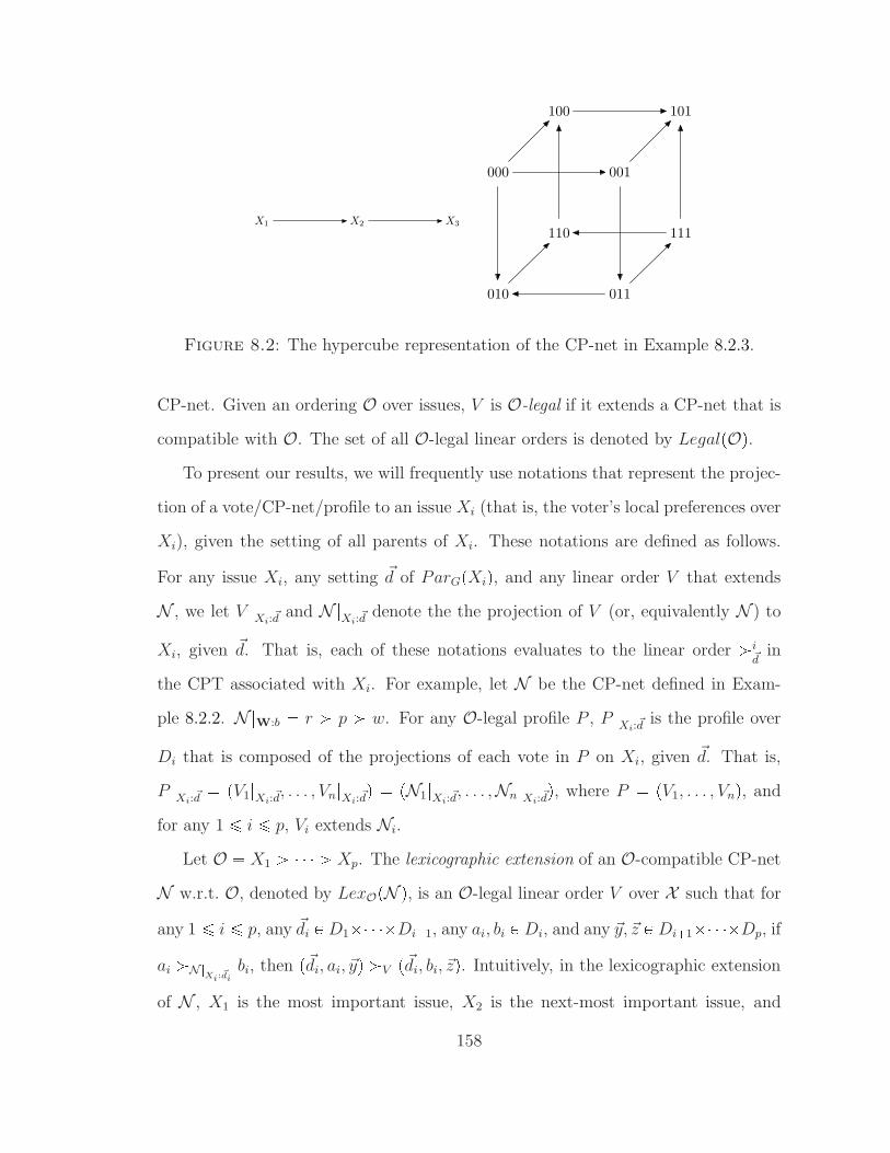
X1 X2 X3
000 001
010 011
100 101
110 111
Figure 8.2: The hypercube representation of the CP-net in Example 8.2.3.
CP-net. Given an ordering O over issues, V is O-legal if it extends a CP-net that is
compatible with O. The set of all O-legal linear orders is denoted by LegalpOq.To present our results, we will frequently use notations that represent the projec-
tion of a vote/CP-net/profile to an issue Xi (that is, the voter’s local preferences over
Xi), given the setting of all parents of Xi. These notations are defined as follows.
For any issue Xi, any setting ~d of ParGpXiq, and any linear order V that extends
N , we let V |Xi:~dand N |Xi:~d
denote the the projection of V (or, equivalently N ) to
Xi, given ~d. That is, each of these notations evaluates to the linear order ¡i~d
in
the CPT associated with Xi. For example, let N be the CP-net defined in Exam-
ple 8.2.2. N |W:b r ¡ p ¡ w. For any O-legal profile P , P |Xi:~d
is the profile over
Di that is composed of the projections of each vote in P on Xi, given ~d. That is,
P |Xi:~d
pV1|Xi:~d, . . . , Vn|Xi:~d
q pN1|Xi:~d, . . . ,Nn|Xi:~d
q, where P pV1, . . . , Vnq, and
for any 1 ¤ i ¤ p, Vi extends Ni.
Let O X1 ¡ ¡ Xp. The lexicographic extension of an O-compatible CP-net
N w.r.t. O, denoted by LexOpN q, is an O-legal linear order V over X such that for
any 1 ¤ i ¤ p, any ~di P D1 Di1, any ai, bi P Di, and any ~y, ~z P Di1 Dp, if
ai ¡N |Xi:
~di
bi, then p~di, ai, ~yq ¡V p~di, bi, ~zq. Intuitively, in the lexicographic extension
of N , X1 is the most important issue, X2 is the next-most important issue, and
158

so on; a desirable change to an earlier issue always outweighs any changes to later
issues. We note that the lexicographic extension of any CP-net is unique w.r.t. the
order O. Again, the subscript “O” is sometimes omitted when there is no risk of
confusion. We say that V P LpX q is lexicographic if it is the lexicographic extension
of a CP-net N . For example, let N be the CP-net defined in Example 8.2.2. We
have LexpN q br ¡ bp ¡ bw ¡ fw ¡ fp ¡ fr ¡ sp ¡ sw ¡ sr. A profile P is
O-legal/separable/lexicographic, if each of its votes is in LegalpOq/ is separable/ is
lexicographic.
8.3 Sequential Voting
One natural approach to combinatorial voting is sequential voting. Let O denote be
an ordering over the issues. W.l.o.g. O X1 ¡ X2 ¡ ¡ Xp. Sequential voting
selects the winner in p rounds. In round i, the voters report their preferences over the
ith issue in O, based on which the winning value is selected by applying a local voting
rule, and this winning value is then announced to all the voters. The idea of sequential
voting is not new. For example, Lacy and Niou (2000) suggested to use sequential
voting to circumvent multiple-election paradoxes. But, again, in the sequential voting
process they proposed, voters are sometimes ill at ease reporting their preferences
over issues, and the voters are still assumed to behave optimistically.3 Moreover,
Lacy and Niou argued that the sequential voting process “takes too long,” because
the voters must wait for the results of previous issues to be announced before moving
to the subsequent issues. They argued that “the cost to voters of going to the polls
and the cost to governments of keeping polls open for several days will likely prevent
the use of sequential voting schemes” (Lacy and Niou, 2000).
In fact, the voters do not need to go to voting booths multiple times. It suffices
3 Lacy and Niou (2000) also suggested to let voters vote strategically and sequentially, and showedthat the outcome will always be the Condorcet winner whenever one exists. This is the strategicsequential voting procedure that will be discussed in Chapter 11.
159

for them to report in one shot all their local preferences over single issues, given
all (relevant) valuations of the previous issues. That is, to apply sequential voting
w.r.t. the order O over issues, it suffices for the voters to use an O-compatible CP-
net to represent their preferences. Of course the voters need to report more of their
preferences, and some of them are not used for the voting rule to decide the winner.
This is not a big problem as long as the language is compact (as we will see later
in this section). Similarly to the situation in issue-by-issue voting (where only the
voters with separable preferences are comfortable with reporting their preferences), in
sequential voting we have a similar criterion: if a voter’s preferences are O-legal, then
she is comfortable with reporting their preferences; otherwise she is not comfortable
with reporting her preferences.
The ground-breaking systematic method for analyzing sequential voting was pro-
posed by Lang (2007), who focused on the profiles where voters are comfortable
reporting their preferences (that is, O-legal profiles), and defined sequential voting
rules on top of these profiles.
Definition 8.3.1. (Lang, 2007) Given a vector of local rules pr1, . . . , rpq, where
for each 1 ¤ i ¤ p, ri is a voting rule on Di, the sequential composition of
r1, . . . , rp w.r.t. O, denoted by SeqOpr1, . . . , rpq, is defined for all O-legal profiles
as follows: SeqOpr1, . . . , rpqpP q pd1, . . . , dpq P X , so that for any 1 ¤ i ¤ p,
di ripP |Xi:d1di1q.
The sequential composition of local correspondences rc1, . . . , r
cp, denoted by
SeqOprc1, . . . , r
cpq, is defined in a similar way: for any O-legal profile P ,
~d P SeqOprc1, . . . , r
cpqpP q if and only if for each i ¤ p, we have that di P rc
i pP |Xi:d1...di1q.
The subscript “O” in SeqO is sometimes omitted when there is no risk of confu-
sion. We note that when a voter’s preferences are O-legal, she only needs to submit
an O-compatible CP-net instead of reporting the entire O-legal linear order. Hence,
160

the voting language used by a sequential rule is essentially the set of all O-compatible
CP-nets. Similarly, the voting language used in issue-by-issue voting is essentially
the set of all separable CP-nets (where there are no edges in the graph). We note that
if the voters’ profile is separable, then sequential voting rules become issue-by-issue
voting rules. In that sense, sequential voting rules are extensions of issue-by-issue
voting rules.
To examine the compactness of the set of all O-compatible CP-nets as a voting
language, let us calculate the size of an O-compatible CP-net (which is the sum of
the sizes of all CPTs). It is easy to see that the size of a CP-net largely depends on
how many parents each issue has in the graph. In fact, the size of a CP-net is
p
i1
¹XjPParGpXiq |Dj| logp|Di|!q
Therefore, if both the number of members in each local domain and the number
of parents for each issue are small, then the size of the CP-net is polynomial in
the number of issues (for comparison, we recall that in multi-issue domains we need
Θpp 2pq bits to represent a linear order, which is exponential in the number of
issues); on the other hand, in the worst case the size of an O-compatible CP-net
is exponentially large in the number of issues. However, in practice it is reasonable
to expect that all local domains are small, and the voters’ preferences over each
issue only depends on a few other issues. Hence, we can expect in practice that
O-compatible CP-nets are a compact language. Obviously O-compatible CP-nets,
as a voting language, are more expressive than the language used by issue-by-issue
voting (that is, separable CP-nets), simply because separable CP-nets are special
cases of O-compatible CP-nets. In fact, it has been shown that the ratio between
the number of O-legal linear orders and the number of separable linear orders is
161

Ωp 2p?πpq (Lang and Xia, 2009), which in some sense shows quantitatively how much
more usable O-compatible CP-nets are, compared to separable CP-nets. Table 8.1
provides a comparison of plurality, common voting rules that require voters to report
linear orders (e.g., Borda), issue-by-issue voting rules, sequential voting rules, the
framework introduced in Chapter 9, and the MLE approach taken in Chapter 10, in
terms of the following three aspects: (1) computational efficiency of computing the
winner, (2) compactness of the voting language, and (3) expressiveness of the voting
language, which includes general usability and informativeness.
Table 8.1: Comparing voting rules and languages for combinatorial voting.
Voting methodComputational
efficiencyCompactness
ExpressivenessGeneral usability Informativeness
Plurality High High High Low
Borda, etc. Low Low High High
Issue-by-issue High High Low Medium
Sequential voting High Usually high Medium Medium
H-compositionin Chapter 9
Low–High(depends on the voters’
common preference
structure)
Usually high High Medium
MLE approachin Chapter 10
Low–High(depends on the
probabilistic model)
Usually high High Medium
For (truthful) sequential voting, multiple-election paradoxes are alleviated (Lacy
and Niou, 2000; Lang and Xia, 2009), though they return when voters vote strategi-
cally, as we will see in Chapter 11. One natural question to ask is whether sequential
voting rules satisfy some other desired axiomatic properties for voting rules (see Sec-
tion 2.2). Not surprisingly, the answer depends on whether the local voting rules
satisfy these axiomatic properties. Lang and Xia (2009) asked the following two
questions for any axiomatic property Y .
162

1. If the sequential voting rule satisfies Y , is it true that all its local voting rules
also satisfy Y ? This corresponds to the “Global to local” column in Table 8.2.
2. If all local voting rules satisfy Y , is it true that their sequential composition
also satisfies Y ? This corresponds to the “Local to global” column in Table 8.2.
The answers for some of the axiomatic properties described in Section 2.2 are sum-
marized in Table 8.2.4
Table 8.2: Local vs. global for sequential rules (Lang and Xia, 2009).
Criteria Global to local Local to globalAnonymity Y YNeutrality Y N
Consistency Y YParticipation Y N
Pareto efficiency Y N(Strong) monotonicity Y Y
For neutrality and Pareto efficiency, Xia and Lang (2009) showed that the ex-
istence of voting correspondences that satisfy neutrality (respectively, Pareto ef-
ficiency) can be characterized by the structure of the multi-issue domain: if the
multi-issue domain is composed of two binary variables, then there exists a voting
correspondence that satisfies neutrality (respectively, Pareto efficiency); otherwise
no voting correspondence satisfies neutrality (respectively, Pareto efficiency).5
Nevertheless, we may still argue that in order for voters to feel comfortable ex-
pressing their preferences, sequential voting is quite restrictive at two levels: first,
at the individual voters’ level, sequential voting requires that a voter’s preferences
must be represented by an acyclic CP-net. Second, at the profile level, it requires
4 Since sequential voting rules are defined for O-legal profiles, the definitions of neutrality, Paretoefficiency, and monotonicity are slightly different. See Lang and Xia (2009).
5 Again, here the definitions of neutrality and efficiency are slightly different from the definitionsin Section 2.2.
163

that all voters’ preferences are compatible with the same ordering O. To overcome
these restrictions, we need to consider even more expressive voting languages. One
option is the set of all (possibly cyclic) CP-nets. Obviously it is more expressive,
because it is a superset of the set of all acyclic CP-nets. Chapters 9 and 10 aim at
designing new voting rules for combinatorial voting where the voters use (possibly
cyclic) CP-nets to represent their preferences. In Chapter 9, we will further show
how much more general (possibly cyclic) CP-nets are, by showing the ratio between
the number of O-legal votes and the number of all linear orders over X (note that
any voter should be comfortable with using a possibly cyclic CP-net to represent
her preferences, in the sense that for any linear order, a possibly cyclic CP-net can
be constructed such that the linear order extends this CP-net). Then, we propose
an extension of sequential voting rules to aggregate (possibly cyclic) CP-nets, which
we call hypercubewise composition (H-composition). We will analyze its normative
and computational aspects. This framework was further studied by Li et al. (2011)
and Conitzer et al. (2011b). In Chapter 10, we extend Condorcet’s MLE model to
combinatorial voting.
Chapters 11 and 12 investigate game-theoretic aspects of combinatorial voting.
In Chapter 11 we study the sequential voting game mentioned by Lacy and Niou
(2000), that is, the game where voters cast votes strategically on one issue after
another, following some ordering over the issues. We call this type of voting games
the strategic sequential voting procedure (SSP). Lacy and Niou (2000) proved that
strategic sequential voting6 always selects the Condorcet winner whenever one exists,
but they did not examine whether there are any multiple-election paradoxes for
SSP. In Chapter 11 we show that all three types of multiple-election paradoxes still
arise in strategic sequential voting. Moreover, changing the ordering of the issues
according to which the voters vote on them cannot avoid at least the first and the
6 They called it sophisticated sequential voting, following the convention of Farquharson (1969).
164

third paradoxes. Then, in Chapter 12, we will see how to restrict voters’ preferences
over multi-issue domains to obtain strategy-proof voting rules.
At the end of this chapter, let me briefly mention some other work in preference
aggregation over multi-issue domains. Rossi et al. (2004) studied aggregating voters’
preferences represented by partial CP-nets, which allows voters to be “indifferent”
with between the values of some issues. Gonzales et al. (2008) studied aggregating
preferences represented by another compact language called GAI-networks. Xia et al.
(2007a) slightly extended sequential voting rules by removing the constraint that
the order O is fixed before the voting process. However, the above two levels of
restrictions for sequential voting rules still exist. Recently, Conitzer et al. (2009a)
studied the agenda control problem in sequential voting—that is, the chair gets to
choose the over in which the issues are voted on, and investigated its computational
complexity.
8.4 Summary
In this chapter, we introduced the notation used in this dissertation for combinatorial
voting, multiple-election paradoxes, CP-nets, sequential voting rules, and important
criteria for designing new voting rules in combinatorial domains. We also evaluated
voting rules proposed in previous work by these criteria, and the result is summarized
in Table 8.1. We observed that all previous approach either used voting languages
that lack expressivity, or is computationally intractable.
165

9
A Framework for Aggregating CP-nets
In this chapter, we define a new family of voting rules for combinatorial voting that
allows voters to use any CP-nets (even cyclic ones) to represent their preferences. The
set of all CP-nets, as a language, is compact and is much more expressive than acyclic
CP-nets or separable CP-nets, which are used in sequential voting and issue-by-issue
voting, respectively.1 The voting rules we define are parameterized by: (1) the local
voting rules that are used on individual attributes—we will use these to define a
particular graph on the set of alternatives; and (2) a choice set function T that selects
the winners based on this induced graph.2 We show that if T satisfies a very natural
assumption, then the voting rules induced by T extend the sequential voting rules
(and therefore, also issue-by-issue voting rules) and the order-independent sequential
composition of local rules from Xia et al. (2007b). We study whether properties of the
local rules transfer to the global rule, and vice versa. Then, we focus on a particular
choice set function, namely the Schwartz set (Schwartz, 1970), which has been argued
1 Earlier work has also considered social choice for potentially cyclic CP-nets (Purrington andDurfee, 2007). However, that approach does not apply to all possible (cyclic) CP-nets.
2 In principle, T could select multiple winners from the graph. We can use any tie-breakingmechanism to select the unique winner.
166
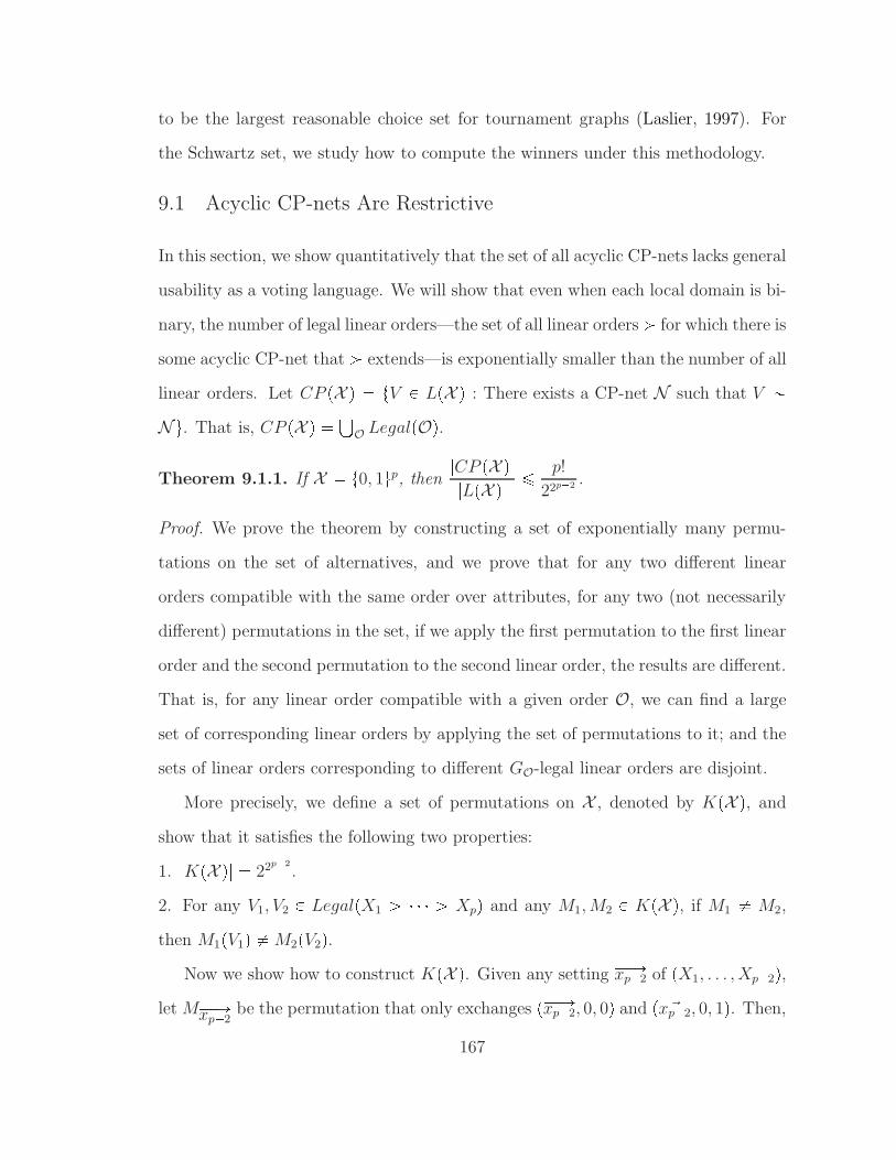
to be the largest reasonable choice set for tournament graphs (Laslier, 1997). For
the Schwartz set, we study how to compute the winners under this methodology.
9.1 Acyclic CP-nets Are Restrictive
In this section, we show quantitatively that the set of all acyclic CP-nets lacks general
usability as a voting language. We will show that even when each local domain is bi-
nary, the number of legal linear orders—the set of all linear orders ¡ for which there is
some acyclic CP-net that ¡ extends—is exponentially smaller than the number of all
linear orders. Let CP pX q tV P LpX q : There exists a CP-net N such that V N u. That is, CP pX q
OLegalpOq.
Theorem 9.1.1. If X t0, 1up, then|CP pX q||LpX q| ¤ p!
22p2.
Proof. We prove the theorem by constructing a set of exponentially many permu-
tations on the set of alternatives, and we prove that for any two different linear
orders compatible with the same order over attributes, for any two (not necessarily
different) permutations in the set, if we apply the first permutation to the first linear
order and the second permutation to the second linear order, the results are different.
That is, for any linear order compatible with a given order O, we can find a large
set of corresponding linear orders by applying the set of permutations to it; and the
sets of linear orders corresponding to different GO-legal linear orders are disjoint.
More precisely, we define a set of permutations on X , denoted by KpX q, and
show that it satisfies the following two properties:
1. |KpX q| 22p2
.
2. For any V1, V2 P LegalpX1 ¡ ¡ Xpq and any M1, M2 P KpX q, if M1 M2,
then M1pV1q M2pV2q.Now we show how to construct KpX q. Given any setting ÝÝÑxp2 of pX1, . . . , Xp2q,
let MÝÝÑxp2be the permutation that only exchanges pÝÝÑxp2, 0, 0q and p ~xp2, 0, 1q. Then,
167

for any Ep2 t0, 1up2, let MEp2 ÝÝÑxp2PEp2
MÝÝÑxp2, where is the composition of
two permutations. This notion is well-defined because for any ÝÝÑxp2,ÝÝÑxp2
1 P t0, 1up2,
MÝÝÑxp2and MÝÝÑxp2
1 are exchangeable, that is, MÝÝÑxp2MÝÝÑxp2
1 MÝÝÑxp21 MÝÝÑxp2
.
Let KpX q tMEp2: Ep2 t0, 1up2u. Then, |KpX q| |t0, 1ut0,1up2 |
22p2
. For any V1, V2 P LegalpX1 ¡ ¡ Xpq any ME1p2
, ME2p2P KpX q such that
ME1p2 ME2
p2, since E1
p2 E2p2, w.l.o.g. there exists ÝÝÑxp2 such that ÝÝÑxp2 P E1
p2
but ÝÝÑxp2 R E2p2. Then, V1|tXp1,Xpu:ÝÝÑxp2
extends a CP-net on t0, 1u2, and the CP-
net is compatible with Xp1 ¡ Xp. Here, V1|tXp1,Xpu:ÝÝÑxp2is the restriction of V1 totXp1, Xpu, given that pX1, . . . , Xp2q ÝÝÑxp2. However, MÝÝÑxp2
pV2q|tXp1,Xpu:ÝÝÑxp2is
not compatible with Xp1 ¡ Xp—it either does not extend a CP-net, or extends a
CP-net that is not compatible with Xp1 ¡ Xp. We note that
ME1p2pV1q|tXp1,Xpu:ÝÝÑxp2
V1|tXp1,Xpu:ÝÝÑxp2,
ME2p2pV2q|tXp1,Xpu:ÝÝÑxp2
MÝÝÑxp2pV2q|tXp1,Xpu:ÝÝÑxp2
Hence, ME1p2pV1q ME2
p2pV2q, which means that KpX q satisfies the two properties
mentioned above.
Therefore, from the two properties of KpX q, we know that |KpX qpLegalpX1 ¡. . . ¡ Xpqq| 22p2|LegalpX1 ¡ . . . ¡ Xpq|. Since KpX qpLegalpX1 ¡ . . . ¡ Xpqq LpX q, and |CP pX q| p!|LpX1 ¡ . . . ¡ Xpq| (because there are p! linear orders
over tx1, . . . , xpu, and a CP-net must be compatible with some order), we have|CP pX q||LpX q| ¤ p!
22p2.
We note that |X | 2p. Theorem 9.1.1 implies that the expressivity ratio of legal
linear orders (|CP pX q||LpX q| ) is Opp20.2q|X |q, which is exponentially small even in the
168

number of alternatives.
9.2 H-Composition of Local Voting Rules
In this section, we introduce a new framework for composing local voting rules. We
call this hypercubewise composition (H-composition) of local voting rules. The reason
is that the outcome only depends on preferences between alternatives that differ on
only one attribute. We can visualize the set of all alternatives as a hypercube, and
alternatives that differ on only one attribute are neighbors on this hypercube, as
discussed in Section 8.2. An H-composition of local rules is defined for all profiles in
which for each vote, there exists a (possibly cyclic) CP-net that it extends. In fact,
for any linear order V on X , there exists a CP-net N such that V extends N , so we
can apply this to any linear orders (but also some partial orders). By Theorem 9.1.1,
this means that the voting language used by these H-compositions (i.e., possibly
cyclic CP-nets) is much more general than the voting language used by sequential
voting rules (i.e., O-compatible CP-nets for some ordering O over I, in the sense we
have discussed in Section 8.3.
An H-composition of local rules is defined in two steps. In the first step, an
induced graph is generated by applying local rules to the input profile. Then, in the
second step, a choice set function is selected based on the induced graph as the set of
winners (the definition and examples of some major choice set functions are deferred
to Definition 9.2.4 and the text below it). We first define the induced graph of P
w.r.t. local rules (or correspondences) r1, . . . , rp.
Definition 9.2.1. Given a profile P pV1, . . . , Vnq and local rules (or correspon-
dences) r1, . . . , rp, the induced graph of P w.r.t. r1, . . . , rp, denoted by IGpr1, . . . , rpqpP q pX , Eq, is defined by the following edges between alternatives. For any i ¤ p, any
setting ÝÑxi, let Ci ripP |Xi:ÝÑxiq; for any ci P Ci, any di P Di, let there be an edge
169

pci,ÝÑxiq Ñ pdi,
ÝÑxiq.Example 9.2.2. Suppose the multi-issue domain consists of two binary attributes: S
ranging over tS, Su and T ranging over tT, T u. The local rules are both the majority
rule. Two votes V1, V2 and their induced graph IGpMaj, MajqpV1, V2q are illustrated
in Figure 9.2.2, where Maj denotes the majority correspondence. We note that V1
is compatible with S ¡ T, V2 is compatible with T ¡ S.
V1 : S ¡ T(S, T ) (S, T )
(S, T ) (S, T )
V2 : T ¡ S(S, T ) (S, T )
(S, T ) (S, T )
Induced graph(S, T ) (S, T )
(S, T ) (S, T )
Figure 9.1: Two votes and their induced graph.
Next, we define the dominance relation in a directed graph.
Definition 9.2.3. Given a directed graph G pV, Eq, for any v1, v2 P V, v1 is said
to dominate v2, denoted by v1 ¡G v2, if and only if:
1. there is a directed path from v1 to v2, and
2. there is no directed path from v2 to v1.
Let ©G be the transitive closure of E, that is, ©G is the minimum preorder such
that if pv1, v2q P E, then v1 ©G v2. Then, another equivalent way to define the
dominance relation is: ¡G is the strict order induced by ©G, that is, v1 ¡G v2 if and
only if v1 ©G v2 and v2 «G v1.
We further define two kinds of special vertices in a directed graph G as follows.
The first is a vertex that dominates all the other vertices, and the second is a vertex
that dominates all its neighbors. We call the former the global Condorcet winner
(which must be unique), and the latter a local Condorcet winner.
170

Now, we are ready to define the choice set function, which specifies a choice set
for each graph.
Definition 9.2.4. A choice set function T is a mapping from any graph to a subset
of its vertices.
We now recall the definitions of some major choice sets in a graph G pV, Eq.• The Schwartz set is the union of all maximal mutually connected subsets. A
maximal mutually connected subset is a subset of vertices such that there is a
path between any two vertices in the set, but there is no path from a vertex
outside the set to a vertex inside the set.
• The Smith set is the smallest set of vertices such that every vertex in the set
dominates all the vertices outside the set.
• The Copeland set: A vertex c’s Copeland score is the number of vertices that
are dominated by c minus the number of vertices that dominate c. The vertices
with the highest Copeland score are the winners.
Choice sets were originally introduced to make group decisions for tournament
graphs. However, the definitions are easily extended to general graphs, as we did
above. See Laffond et al. (1995) and Brandt et al. (2007) for more discussion.
We say a choice set function T always chooses the global Condorcet winner, if for
any graph G pV, Eq in which c is the global Condorcet winner, we have T pGq tcu.We say that T always chooses local Condorcet winners, if every local Condorcet
winner is always in T pGq. We emphasize that here, the meaning of a Condorcet
winner is different from traditional meaning of a Condorcet winner, which refers to
an alternative that wins every pairwise election. We say that T is monotonic, if for
any graph pV, Eq, any c P T pV, Eq, and any pV, E 1q that is obtained from pV, Eq by
only flipping some of the incoming edges of c, we have c P T pV, E 1q.171
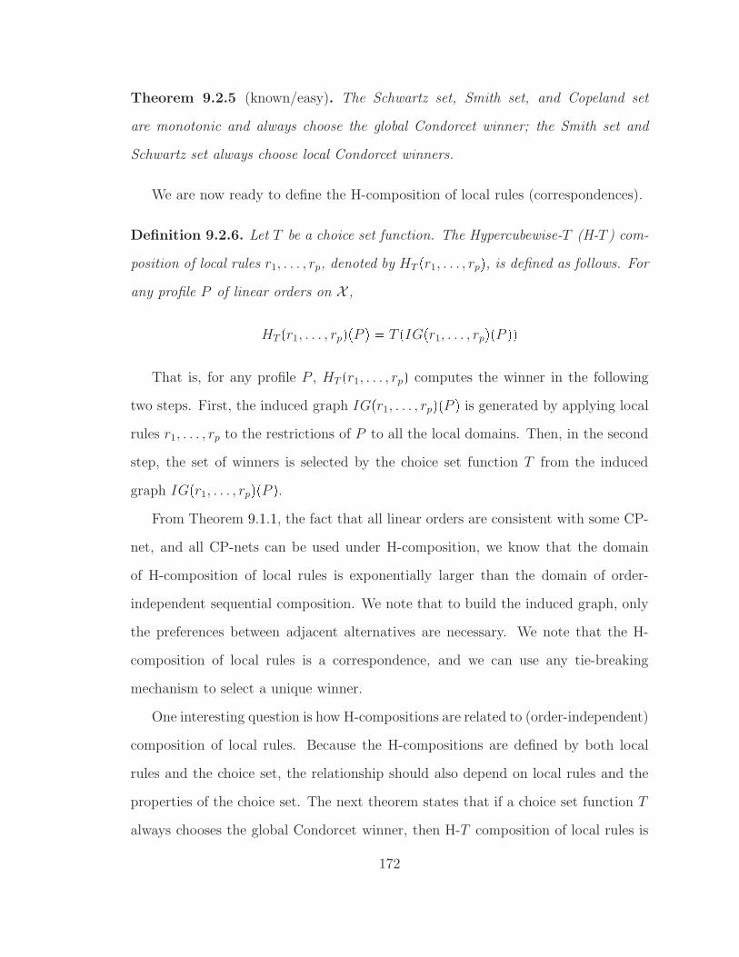
Theorem 9.2.5 (known/easy). The Schwartz set, Smith set, and Copeland set
are monotonic and always choose the global Condorcet winner; the Smith set and
Schwartz set always choose local Condorcet winners.
We are now ready to define the H-composition of local rules (correspondences).
Definition 9.2.6. Let T be a choice set function. The Hypercubewise-T (H-T ) com-
position of local rules r1, . . . , rp, denoted by HT pr1, . . . , rpq, is defined as follows. For
any profile P of linear orders on X ,
HT pr1, . . . , rpqpP q T pIGpr1, . . . , rpqpP qqThat is, for any profile P , HT pr1, . . . , rpq computes the winner in the following
two steps. First, the induced graph IGpr1, . . . , rpqpP q is generated by applying local
rules r1, . . . , rp to the restrictions of P to all the local domains. Then, in the second
step, the set of winners is selected by the choice set function T from the induced
graph IGpr1, . . . , rpqpP q.From Theorem 9.1.1, the fact that all linear orders are consistent with some CP-
net, and all CP-nets can be used under H-composition, we know that the domain
of H-composition of local rules is exponentially larger than the domain of order-
independent sequential composition. We note that to build the induced graph, only
the preferences between adjacent alternatives are necessary. We note that the H-
composition of local rules is a correspondence, and we can use any tie-breaking
mechanism to select a unique winner.
One interesting question is how H-compositions are related to (order-independent)
composition of local rules. Because the H-compositions are defined by both local
rules and the choice set, the relationship should also depend on local rules and the
properties of the choice set. The next theorem states that if a choice set function T
always chooses the global Condorcet winner, then H-T composition of local rules is
172
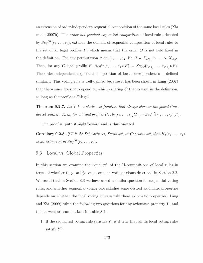
an extension of order-independent sequential composition of the same local rules (Xia
et al., 2007b). The order-independent sequential composition of local rules, denoted
by SeqOIpr1, . . . , rpq, extends the domain of sequential composition of local rules to
the set of all legal profiles P , which means that the order O is not held fixed in
the definition. For any permutation σ on t1, . . . , pu, let O Xσp1q ¡ . . . ¡ Xσppq.Then, for any O-legal profile P , SeqOIpr1, . . . , rpqpP q SeqOprσp1q, . . . , rσppqqpP q.The order-independent sequential composition of local correspondences is defined
similarly. This voting rule is well-defined because it has been shown in Lang (2007)
that the winner does not depend on which ordering O that is used in the definition,
as long as the profile is O-legal.
Theorem 9.2.7. Let T be a choice set function that always chooses the global Con-
dorcet winner. Then, for all legal profiles P , HT pr1, . . . , rpqpP q SeqOIpr1, . . . , rpqpP q.The proof is quite straightforward and is thus omitted.
Corollary 9.2.8. If T is the Schwartz set, Smith set, or Copeland set, then HT pr1, . . . , rpqis an extension of SeqOIpr1, . . . , rpq.9.3 Local vs. Global Properties
In this section we examine the “quality” of the H-compositions of local rules in
terms of whether they satisfy some common voting axioms described in Section 2.2.
We recall that in Section 8.3 we have asked a similar question for sequential voting
rules, and whether sequential voting rule satisfies some desired axiomatic properties
depends on whether the local voting rules satisfy these axiomatic properties. Lang
and Xia (2009) asked the following two questions for any axiomatic property Y , and
the answers are summarized in Table 8.2.
1. If the sequential voting rule satisfies Y , is it true that all its local voting rules
satisfy Y ?
173

2. If the sequential voting rule satisfies Y , is it true that all its local voting rules
satisfy Y ?
For H-composition of local rules, we can ask the same question. From Theo-
rem 9.2.7 we know that if T always chooses the global Condorcet winner, then HT is
an extension of SeqOI . We can use this observation to carry over some of the results
in Lang (2007); Xia et al. (2007a,b) to HT . Specifically, if T always chooses the global
Condorcet winner, and if a criterion transfers from the order-independent sequential
composition of local rules to each local rule, then it also transfers for H-T compo-
sition; if a criterion does not transfer from local rules to their order-independent
sequential composition, then it also does not transfer for H-T composition. Given
the results in Xia et al. (2007b), these observations allow us to resolve everything ex-
cept how anonymity, homogeneity, monotonicity, and consistency transfer from local
rules to their H-T composition. It is easy to see that anonymity and homogeneity
always transfer. The next example shows that if T always chooses local Condorcet
winners, then consistency does not transfer, even when the votes in the profile extend
(possibly different) acyclic CP-nets.
Example 9.3.1. Let X t01, 11u t02, 12u t03, 13u, and let all the local rules be
the majority rule. Consider the following three CP-nets (the non-specified parts of
the CPTs do not matter):
N1: compatible with X1 ¡ X2 ¡ X3, and 11 ¡ 01, 11 : 12 ¡ 02, 1112 : 13 ¡ 03,
01 : 02 ¡ 12, 0102 : 03 ¡ 13.
N2: compatible with X2 ¡ X3 ¡ X1, and 12 ¡ 02, 12 : 13 ¡ 03, 1213 : 11 ¡ 01,
02 : 03 ¡ 13, 0203 : 01 ¡ 11.
N1: compatible with X3 ¡ X1 ¡ X2, and 13 ¡ 03, 13 : 11 ¡ 01, 1311 : 12 ¡ 02,
03 : 01 ¡ 11, 0301 : 02 ¡ 12.
174

For any V1, V2, V3 extending N1,N2,N3, respectively, let P pV1, V2, V3q. Let
HT pMq HT pMaj, Maj, Majq. Suppose ties are broken in favor of 010203. Because
010203 is a local Condorcet winner, so HT pMqpP q 010203. However, HT pMqpV1q HT pMqpV2q HT pMqpV3q 111213, so HT pMq does not satisfy consistency (because
otherwise, we must have HT pMq 111213, which we know is not the case).
The next proposition states that for any monotonic choice set function T , the
monotonicity is transferred from local rules to their H-T composition. The proof is
quite straightforward and is omitted.
Proposition 9.3.2. Let T be a monotonic choice set function. If all local rulestr1, . . . , rpu satisfy monotonicity, then HT pr1, . . . , rpq also satisfies monotonicity.
For choice sets T that always choose the global Condorcet winner, whether prop-
erties of local rules transfer to their H-T composition and vice versa is summarized
in Table 9.1.
Table 9.1: Local vs. global for H-compositions.
Criteria Global to local Local to global
Anonymity Y Y
Homogeneity Y Y
Neutrality Y N
Monotonicity Y Y for monotonic T
Consistency Y N if T always chooseslocal Condorcet winner
Participation Y N
Pareto efficiency Y N
9.4 Computing H-Schwartz Winners
Among all choice sets, we are most interested in the Schwartz set, because first,
it has been argued that the Schwartz set is the “largest” reasonable choice set for
tournaments (Laslier, 1997), and second, it corresponds to the nondominated set pre-
viously considered in the context of CP-nets (Boutilier et al., 2004). In this section,
175

we investigate the computational complexity of computing H-Schwartz winners. We
note that in this section H-Schwartz is a voting correspondence. Recent work on the
complexity of computing dominance relations in CP-nets shows that the dominance
problem in a CP-net is hard (Goldsmith et al., 2008). More precisely, given a CP-net
N and two alternatives a and b, it is PSPACE-complete to compute whether or not
a ¡N b. This can be used to show that checking membership in the Schwartz set is
PSPACE-complete (Goldsmith et al., 2008).
Although computing the Schwartz set is hard in general, if the preferences are
more structured it can be easy. As an extreme example, if the voters’ preferences
extend an acyclic CP-net N , then H-Schwartz is equivalent to order-independent
sequential composition of local rules, under which computing the winner is easy. In
this section, we introduce a technique to exploit more limited independence infor-
mation in the submitted votes for the purpose of computing the set of H-Schwartz
winners.
Definition 9.4.1. Let tI1, . . . , Iqu (q ¤ p) be a partition of the set of issues I. We
say a CP-net N whose graph is G is compatible with the ordering I1 ¡ ¡ Iq
if for any l ¤ q and any X P Il, ParGpXq I1 Y . . . Y Il. A linear order V is
compatible with I1 ¡ . . . ¡ Iq if there exists a CP-net N such that V extends N and
N is compatible with I1 ¡ . . . ¡ Iq.
Let O X1 ¡ . . . ¡ Xp. One special case is the following: if the input profile
is O-legal, then we can use the partition I1 tX1u, . . . , Ip tXpu. We can use the
following algorithm to find a partition with which the input profile P is compatible.
Suppose that we already know the graphs of the CP-nets that the votes in P extend.
Algorithm 1
1. Let GP be the union of all the graphs of the CP-nets that the votes in P extend.
2. Let q 0; repeat step 3 until GP H.
176

3. Let q q 1. Find a maximal mutually connected subset of GP , and call it Iq.
Remove Iq and all edges connecting it to GP .
4. Output the partition I1 Y . . .Y Iq.
This algorithm runs in time Opp3q. Now we are ready to present the technique
for computing the set of H-Schwartz winners more efficiently. Suppose the set of
attributes can be partitioned into I1 Y I2 so that P is compatible with I1 ¡ I2. Let
rI1denote the sub-vector of pr1, . . . , rpq that contains the local rules ri if and only if
Xi P I1.
Process 1
1. Compute the Schwartz set HSchwartzprI1qpP |I1
q W 11 Y . . .YW k
1 , where the W i1
are the maximal mutually connected subsets in IGprI1qpP |I1
q.2. For each i ¤ k, let IGprI2
qpP |I2:W i1q ~wPW i
1
IGprI2qpP |I2:~wq; then, compute the
Schwartz set W i2 for IGprI2
qpP |I2:W i1q.
3. Output Wp k
i1 W i1 W i
2.
The next theorem states that we can compute the winners of HSchwartzpr1, . . . , rpqpP qby Process 1.
Theorem 9.4.2. WP HSchwartzpr1, . . . , rpqpP q.Proof. Let ~w2 be a setting of I2 and ~w1, ~w11 be settings of I1 such that ~w1 and ~w11differ only on one attribute. Since P is compatible with I1 ¡ I2, we have that there
is an edge from p~w1, ~w2q to p~w11, ~w2q in IGprIqpP q if and only if there is an edge from
~w1 to ~w11 in IGprI1qpP |I1
q. This implies the following claim.
Claim 9.4.1. If there is a path from p~w1, ~w2q to p~w11, ~w12q in IGprIqpP q, then its
projection on I1 is a path from ~w1 to ~w11 in IGprI1qpP |I1
q.Proof of Claim 9.4.1: W.l.o.g. we only need to prove the case where there is an
edge from p~w1, ~w2q to p~w11, ~w12q in IGprIqpP q. Because only neighboring alternatives
177
are connected in IGprIqpP q, either ~w1 ~w11 or ~w2 ~w12. If ~w1 ~w11 then the
claim is automatically proved, because the projections of the two alternatives in
IGprI1qpP |I1
q are the same (that is, ~w1). If ~w2 ~w12, then by definition there is an
from ~w1 to ~w11 in IGprI1qpP |I1
q. This proves the claim. lWe note that for any i ¤ k, any ~w1, ~w11 P W i
1 such that there is a path from ~w1 to
~w11, and any ~w2 P DI2, there is a path from p~w1, ~w2q to p~w11, ~w2q. Therefore, we have
the following claim.
Claim 9.4.2. For any i ¤ k, any p~w1, ~w2q, p~w11, ~w12q P W i1DI2
, there is a path fromp~w1, ~w2q to p~w11, ~w12q if and only if there is a path from ~w2 to ~w12 in IGprI2qpP |I2:W i
1q.
Proof of Claim 9.4.2: We first prove the “only if” part. W.l.o.g. we only need
to prove the case where there is an edge from p~w1, ~w2q to p~w11, ~w12q in IGprIqpP q.In this case either ~w1 ~w11 or ~w2 ~w12. If ~w1 ~w11, then there is an edge from
~w2 to ~w12 in IGprI2qpP |I2:~w1
q, which means that there is an edge from ~w2 to ~w12 in
IGprI2qpP |I2:W i
1q. If ~w2 ~w12, then the claim is automatically proved.
Now we prove the “if” part. W.l.o.g. we only need to prove the case where there
is an edge from ~w2 to ~w12 in IGprI2qpP |I2:W i
1q. By definition of IGprI2
qpP |I2:W i1q, there
exists ~w1 P W i1 such that there is an edge from ~w2 to ~w12 in IGprI2
qpP |I2:~w1q, which
means that there is an edge from p~w1 , ~w2q to p~w1 , ~w12q in IGprIqpP q. Because W i1 is a
maximum mutually connected set, there exist a path from ~w1 to ~w1 and another path
from ~w1 to ~w11 in IGprI1qpP |I1
q. Because P is compatible with I1 ¡ I2, there exist
two paths in IGprIqpP q, one from p~w1, ~w2q to p~w1 , ~w2q and the other from p~w1 , ~w12qto p~w11, ~w12q. These two paths can be connected by the edge from p~w1 , ~w2q to p~w1 , ~w12qto form a path from p~w1, ~w2q to p~w11, ~w12q. l
Based on Claim 9.4.1 and Claim 9.4.1 we are now ready to prove that WP HSchwartzprIqpP q and HSchwartzprIqpP q WP , which mean that WP HSchwartzprIqpP q.
We first prove that WP HSchwartzprIqpP q. Equivalently, we need to prove that
178
for any p~w1, ~w2q P WP , there is no alternative p~w11, ~w12q P X such that (1) there is a
path from p~w11, ~w12q to p~w1, ~w2q, (2) there is no path from p~w1, ~w2q to p~w11, ~w12q. We
prove this by contradiction. Suppose there exists p~w11, ~w12q that satisfies the above
two conditions. Suppose ~w1 P W i1. By Claim 9.4.1, there is a path from ~w11 to ~w1
in IGprI1qpP |I1
q. Because W i1 is a maximum mutually connected set, ~w11 P W i
1. By
Claim 9.4.2 there exists a path from ~w12 to ~w2 in IGprI2qpP |I2:W i
1q. Because ~w2 P W i
2,
there must exist a path from ~w2 to ~w12 in IGprI2qpP |I2:W i
1q. Now, by Claim 9.4.2 there
exists a path from p~w1, ~w2q to p~w11, ~w12q, which contradicts the condition (2) above.
Next, we prove that HSchwartzprIqpP q WP . Let p~w1, ~w2q P HSchwartzprIqpP q.We first show that ~w1 P HSchwartzprI1
qpP |I1q. Suppose for the sake of contradic-
tion ~w1 R HSchwartzprI1qpP |I1
q, then there exists ~w11 P DI1such that (1) there is a
path from ~w11 to ~w1 in IGprI1qpP |I1
q, and (2) there is no path from ~w1 to ~w11 in
IGprI1qpP |I1
q. From (1) we know that there is a path from p~w11, ~w2q to p~w1, ~w2q.From (2) we know that there is no path from p~w1, ~w2q to p~w11, ~w2q, because other-
wise by Claim 9.4.1 there is a path from ~w1 to ~w11, which is a contradiction. It
follows that p~w1, ~w2q is dominated by p~w11, ~w2q, which contradicts the assumption
that p~w1, ~w2q P HSchwartzprIqpP q. Therefore, ~w1 P HSchwartzprI1qpP |I1
q.Now, suppose ~w1 P W i
1. If ~w2 R W i2, then there exists ~w12 P W i
2 that dominates ~w2.
However, it follows from Claim 9.4.2 that p~w1, ~w12q dominates p~w1, ~w2q in IGprIqpP q,which contradicts the assumption that p~w1, ~w2q P HSchwartzprIqpP q. It follows that
~w2 P W i2, which means that p~w1, ~w2q P WP .
Therefore, WP HSchwartzprIqpP q, which completes the proof.
If the decomposition is I1 ¡ . . . ¡ Iq with q ¡ 2, then Process 1 can be applied
recursively to find the Schwartz set, as follows. First, compute the Schwartz set
over I1 I2 by Process 1, then use this result to compute the Schwartz set overpI1 I2q I3, etc. up to pI1 . . . Iq1q Iq.
179

The next example shows how Process 1 works.
Example 9.4.3. Let X t0, 1u3, and let three votes V1, V2, V3 extend three CP-nets
such that V1 is pX1 ¡ X2 ¡ X3q-legal, V2 is pX2 ¡ X1 ¡ X3q-legal, and V3 is sep-
arable. Let the partition be I1 tX1, X2u, I2 tX3u. Then, for all i 1, 2, 3,
Vi is compatible with I1 ¡ I2. Suppose that t~w1, ~w11u HSchwartzpr1, r2qpP |tX1,X2uq,so that there is no path from ~w1 to ~w11, and vise versa. Also suppose that t~w2u HSchwartzpr3qpP |X3:X3~w1
q and t~w12u HSchwartzpr3qpP |X3:X3~w11q. Then, the win-
ners are p~w1, ~w2q and p~w11, ~w12q.The next theorem states that if P is compatible with I1 ¡ . . . ¡ Iq, then the
time required to compute the set of Schwartz winners by applying Process 1 is a
polynomial function of the number of winners, the longest time it takes to apply
local rules, p, n, and max |DIi|.
Theorem 9.4.4. Suppose an n-vote profile P is compatible with I1 ¡ . . . ¡ Iq. Let
dmax maxi¤q |DIq |. Let tmaxpnq be the longest time it takes to apply local rules on
n inputs. Then, the running time of Process 1 is Opapdmaxpnp tmaxpnqp dmaxqq,where a is the number of H-Schwartz winners.
Usually tmaxpnq is polynomial. Therefore, the computational complexity of Pro-
cess 1 mainly comes from the number of H-Schwartz winners, and the size of the
largest partition dmax.
9.5 Summary
Sequential voting rules require the voters’ preferences to extend acyclic CP-nets
compatible with a common order on the attributes. We showed that this requirement
is very restrictive, by proving that the number of linear orders extending an acyclic
CP-net is exponentially smaller than the number of all linear orders. This means
180

that the voting language used in sequential voting rules lacks general usability. To
overcome this, in this chapter we introduced a very general methodology that allows
us to aggregate preferences when voters express CP-nets that can be cyclic. There
does not need to be any common structure among the submitted CP-nets. We
studied whether properties of the local rules transfer to the global rule, and vice
versa. We also addressed how to compute the winning alternatives.
181

10
A Maximum-Likelihood Approach
In voting, the joint decision is made based on the agents’ preferences. Therefore,
in some sense, this means that the agents’ preferences are the “causes” of the joint
decision. However, there is a different (and almost reversed) point of view: there is
a “correct” joint decision, but the agents may have different perceptions (estimates)
of what this correct decision is. Thus, the agents’ preferences can be viewed as noisy
reports on the correct joint decision. Even in this framework, the agents still need to
make a joint decision based on their preferences, and it makes sense to choose their
best estimate of the correct decision. Given a noise model, one natural approach is
to choose the maximum likelihood estimate of the correct decision. The maximum
likelihood estimator is a function from profiles to alternatives (more accurately, sub-
sets of alternatives, since there may be ties), and as such is a voting rule (more
accurately, a correspondence).
This maximum likelihood approach was first studied by Condorcet (1785) for the
cases of two and three alternatives. Much later, Young (1995) and Young (1988)
showed that for arbitrary numbers of alternatives, the MLE rule derived from Con-
dorcet’s noise model coincides with Kemeny’s rule (Kemeny, 1959). The approach
182
was further pursued by Drissi-Bakhkhat and Truchon (2004). More recently, Conitzer
and Sandholm (2005a) studied whether and how common voting correspondences can
be represented as maximum likelihood estimators. Truchon (2008) studied a differ-
ent way of viewing Borda as an MLE. We studied the relationship between MLEs
and ranking scoring rules (Conitzer et al., 2009b). Conitzer (2011) took an MLE
approach towards voting in social networks. We studied an MLE approach towards
voting with partial orders Xia and Conitzer (2011b). The related notion of dis-
tance rationalizability has also received attention in the computational social choice
community recently (Elkind et al., 2009a).
All of the above work does not assume any structure on the set of alternatives.
In this chapter, we take an MLE approach to preference aggregation in multi-issue
domains, when the voters’ preferences are represented by (not necessarily acyclic)
CP-nets. Considering the structure of CP-nets, we focus on probabilistic models
that are very weakly decomposable. That is, given the “correct” winner, a voter’s
local preferences over an issue are independent from her local preferences over other
issues, and as well as from her local preferences over the same issue given a different
setting of (at least some of) the other issues.
After reviewing some background, we start with the general case in which the
issues are not necessarily binary. The goal here is to investigate when issue-by-
issue or sequential voting rules can be modeled as maximum likelihood estimators.
When the input profile is separable, we completely characterize the set of all voting
correspondences that can be modeled as an MLE for a noise model satisfying a weak
decomposability (respectively, strong decomposability) property. Then, when the
input profile of CP-nets is compatible with a common order over issues, we prove
that no sequential voting rule satisfying unanimity can be represented by an MLE,
provided the noise model satisfies very weak decomposability. We show that this
impossibility result no longer holds if the number of voters is bounded above by a
183

constant.
Then, we move to the special case in which each issue has only two possible
values. For such domains, we introduce distance-based noise models, in which the
local distribution over any issue i under some setting of the other issues depends only
on the Hamming distance from this setting to the restriction of the “correct” winner
to the issues other than i. We characterize distance-based noise models axiomatically.
Then we focus on distance-based threshold noise models in which there is a threshold
such that if the distance is smaller than the threshold, then a fixed nonuniform local
distribution is used, whereas if the distance is at least as large as the threshold, then
a uniform local distribution is used. We show that when the threshold is one, it is
NP-hard to compute the winner, but that when it is equal to the number of issues,
the winner can be computed in polynomial time.
10.1 Maximum-Likelihood Approach to Voting in Unstructured Do-mains
In the maximum likelihood approach to voting, it is assumed that there is a correct
winner d P C, and each vote V is drawn conditionally independently given d, accord-
ing to a conditional probability distribution πpV |dq. The independence structure of
the noise model is illustrated in Figure 10.1. The use of this independence structure
is standard. Moreover, if conditional independence among votes is not required, then
any voting rule can be represented by an MLE for some noise model (Conitzer and
Sandholm, 2005a), which trivializes the question.
Under this independence assumption, the probability of a profile P pV1, . . . , Vnqgiven the correct winner d is πpP |dq ±n
i1 πpVi|dq. Then, the maximum likelihood
estimate of the correct winner is MLEπpP q arg maxdPC πpP |dq.MLEπ is a voting correspondence, as there may be several alternatives d that
maximize πpP |dq. Of course we can turn it into a voting rule by using a tie-breaking
184

“correct” outcome
Voter 1 Voter 2 Voter n. . .
Figure 10.1: The noise model.
mechanism, but for most part of this chapter, we will study the properties of MLE
correspondences. Another model that has been studied assumes that there is a
correct ranking of the alternatives. Here, the model is defined similarly: given the
correct linear order V , each vote V is drawn conditionally independently according
to πpV |V q. The maximum likelihood estimate is defined as follows.
MLEπpP q arg maxV PLpCq¹
V PP πpV |V qIn this chapter, we require that all such conditional probabilities to be positive
for technical reasons.
Definition 10.1.1. (Conitzer and Sandholm, 2005a). A voting rule (correspon-
dence) r is a maximum likelihood estimator for winners under i.i.d. votes (MLEWIV)
if there exists a noise model π such that for any profile P , we have that MLEπpP q rpP q.
Conitzer and Sandholm (2005a) studied which common voting rules/correspondences
are MLEWIVs.
10.2 Multi-Issue Domain Noise Models
In this section, we extend the maximum-likelihood estimation approach to multi-
issue domains (where X D1 . . . Dp). For now, we consider the case where
there is a correct winner, ~d P X . We let the voting language to be the set of all
185
(possibly cyclic) CP-nets, that is, votes are given by CP-nets and are conditionally
independent, given ~d. Let CPnetpX q denote the set of all (possibly cyclic) CP-nets
over X . The probability of drawing CP-net N given that the correct winner is ~d is
πpN |~dq, where π is some noise model. We note that π is a conditional probability
distribution over all CP-nets (in contrast to all linear orders in previous studies).
Given this noise model, for any profile of CP-nets PCP pN1, . . . ,Nnq, the maximum
likelihood estimate of the correct winner is
MLEπpP q arg max~dPX n¹
j1
πpNj|~dqAgain, MLEπ is a voting correspondence.
Even if for all i, |Di| 2, the number of CP-nets (including cyclic ones) is 2p2p1
(2 options for each entry of each CPT, and the CPT of any issue i has 2p1 entries,
one for each setting of the issues other than i). Hence, to specify a probability
distribution over CP-nets, we will assume some structure in this distribution so that
it can be compactly represented. Throughout the chapter, we will assume that the
local preferences for individual issues (given the setting of the other issues) are drawn
conditionally independently, both across issues and across settings of the other issues,
given the correct winner. More precisely:
Definition 10.2.1. A noise model is very weakly decomposable if for every ~d P X ,
every i ¤ p, and every ~ai P Di, there is a probability distribution π~ai
~dover LpDiq,
so that for every ~d P X and every N P CPnetpX q, πpN |~dq ±i¤p,~aiPDiπ
~ai
~dpN |Xi:~ai
qFor instance, if Di t0i, 1i, 2iu, π
~ai
~dp0i ¡ 2i ¡ 1iq is the probability that the
CP-net of a given voter contains ~ai : 0i ¡ 2i ¡ 1i, given that the correct winner is ~d.
Then, the probability of CP-net N is the product of the probabilities of all its local
preferences N |Xi:~aiover specific Xi given specific ~ai (which contains the setting
186

for Xi’s parents as a sub-vector), when the correct winner is ~d. (We will introduce
stronger decomposability notions soon.)
Assuming very weak decomposability is reasonable in the sense that a voter’s
preferences for one issue are not directly linked to her preferences for another issue.
We note that this is completely different from saying that the voter’s preferences
for an issue do not depend on the values of the other issues. Indeed, the voter’s
preferences for an issue can, at least in principle, change drastically depending on
the values of the other issues. For instance, in Example 8.2.2, the event “the voter
prefers white to pink to red wine when the main course is fish” is probabilistically
independent (conditional on the correct outcome) of the event “the voter prefers beef
to salad to fish when the wine is red.”
However, we do not want to argue that such a distribution always generates
realistic preferences. In fact, with some probability, such a distribution generates
cyclic preferences. This is not a problem, in the sense that the purpose of the
maximum likelihood approach is to find a natural voting rule that maps profiles to
outcomes. The fact that this rule is also defined for cyclic preferences does not hinder
its application to acyclic preferences. Similarly, Condorcet’s original noise model for
the single-issue setting also generates cyclic preferences with some probability, but
this does not prevent us from applying the corresponding (Kemeny) rule (Kemeny,
1959) to acyclic preferences.
Even assuming very weak decomposability, we still need to define exponentially
many probabilities. We will now introduce some successive strengthenings of the
decomposability notion. First, we introduce weak decomposability, which removes
the dependence of an issue’s local distribution on the settings of the other issues in
the correct winner.
Definition 10.2.2. A very weakly decomposable noise model π is weakly decompos-
187

able if for any i ¤ p, any ~d1, ~d2 P X such that ~d1|Xi ~d2|Xi
, we must have that for
any ~ai P Di, π~ai
~d1
π~ai
~d2
. Here ~d1|Xiis the Xi-component of ~d1.
Next, we introduce an even stronger notion, namely strong decomposability, which
removes all dependence of an issue’s distribution on the settings of the other issues.
That is, the local distribution only depends on the value of that issue in the correct
winner.
Definition 10.2.3. A very weakly decomposable noise model π is strongly decom-
posable if it is weakly decomposable, and for any i ¤ p, any ~ai,~bi P Di, any
~d P X , we must have that π~ai
~d π
~bi
~d.
10.3 Characterizations of MLE correspondences
It seems that the MLE approaches are quite different from the voting rules that
have previously been studied in the context of multi-issue domains, such as issue-
by-issue voting and sequential voting. This may imply that the maximum likelihood
approach can generate sensible new rules for multi-issue domains. Nevertheless, we
may wonder whether previously studied rules also fit under the MLE framework.
In this section, we study whether or not issue-by-issue and sequential voting
correspondences can be modeled as the MLEs for very weakly decomposable noise
models. We note that even though MLEs for very weakly decomposable noise models
are defined over profiles of CP-nets, they can be easily extended to deal with profiles
of linear orders in the following way. For each linear order Vj in the input profile P ,
let Nj denote the CP-net (possibly cyclic) that Vj extends. Then, we apply the MLE
rule to select winner(s) from pN1, . . . ,Nnq. We recall that voting rules (which always
output a unique winner) are a special case of voting correspondences. Therefore,
our results easily extend to the case of voting rules. First, we restrict the domain
to separable profiles, and characterize the set of all correspondences that can be
188

modeled as the MLEs for strongly/weakly decomposable noise models.
Theorem 10.3.1. Over the domain of separable profiles, a voting correspondence rc
can be modeled as the MLE for a strongly decomposable noise model if and only if rc
is an issue-by-issue voting correspondence composed of MLEWIVs.
Proof of Theorem 10.3.1: First we prove the “if” part. Let rc be an issue-by-
issue voting correspondence that is composed of rc1, . . . , r
cp, in which for any i ¤ p, rc
i
is an MLEWIV over Di of the noise model PrpV i|diq, where V i P LpDiq and di P Di.
Let π be a noise model over X defined as follows: for any i ¤ p, any ~d P X , any
~ai P Di and any V i P LpDiq, we have that π~a~dpViq PrpV i|diq. We next prove that
for any separable profile P , we must have that MLEπpP q rcpP q.MLEπpP q arg max
~d
¹i¤p,~aiPDi
n¹j1
π~ai
~dpVjq arg max
~d
¹i¤p
n¹j1
PrppVi|Xiq|diq|Di|
Therefore, ~b P MLEπpP q if and only if for any i ¤ p, we have
bi P arg maxdi
n¹j1
PrppVi|Xiq|biq
We note that for any ~d1 P rpP q, we must have that d1i arg maxdi
±n
j1 PrppVi|Xiq|diq.
Therefore, ~d1 P MLEπpP q.Next, we prove the “only if” part. For any MLEπ where π is strongly decom-
posable, we define an issue-by-issue voting rule as follows: for any i ¤ p, let rci be
the MLEWIV that corresponds to the noise model in which for any di P Di, we have
that PrpV i|diq π~ai
~dpV iq. Similar to the proof for the “if” part, we have that rc
and MLEπ are equivalent over the domain of separable profiles. l189

A candidate scoring correspondence c is a correspondence defined by a scoring
function s : LpX q X Ñ R in the following way: for any profile P , cpP q arg maxdPX °V PP spV, dq.Theorem 10.3.2. Over the domain of separable profiles, a voting correspondence rc
can be modeled as the MLE for a weakly decomposable noise model if and only if rc
is an issue-by-issue voting correspondence composed of candidate scoring correspon-
dences.
Proof of Theorem 10.3.2: First we prove the “if” part. Let rc be an issue-by-
issue voting correspondence in which the issue-wise correspondence over Di is rcsi,
which has scoring function si. Let π~ai
didenote π
~ai
~d, where the ith component of ~d is
di. Because r is strongly decomposable, π~ai
diis well-defined. For any i ¤ p, we claim
that there exists a set of probability distributions π~ai
~d, ~d P X ,~ai P Di over LpDiq
such that for any di P Di, di P arg maxbiPDi
±n
j1
±~aiPDi
π~ai
bipVj |Xi
q if and only if
di P rcsipP |Xi
q.We note that for any scoring function s and any constant t, the ranking scoring
rule that corresponds to s is equivalent to the ranking scoring rule that corresponds
to s t. Therefore, without loss of generality we let sipV i, diq 0 for any i ¤ p, any
V i P LpDiq, and any di P Di. Let Ki |Di|, LpDiq tl1, . . . , lKi!u.Claim 10.3.1. There exist ki, ti P R with ki ¡ 0, such that for any V i P LpDiq and
any di P Di, we have that lnp±~diPDiπ
~di
dipV iqq kisipV i, diq ti.
Proof of Claim 10.3.1: We let ki be a real number such that for any di P Di, we
have that°Ki!
j1pexppsiplj, diqqqki 1; let pjdi exppsiplj, diqq. For any di P Di, any
190

1 ¤ α Ki!
Ki! 1, we let
fdipαq lnpp1 Ki!1
j1
pjdi
αqp1 pKi 1q α
Ki!qq
Because°Ki!
j1 pjdi 1, we have that lnp1 °Ki!1
j1 pjdiq ¡ ln pKi!
di kisiplKi!, diq.
Therefore, fdip1q ¥ kisiplKi!, diq lnpKi!q. We note that lim
ॠKi!
Ki!1
fdipαq 8. It
follows that there exists 1 ¤ αdi¤ Ki!
Ki! 1such that fdi
pαdiq kisiplKi!, diqlnpKi!q.
For any i ¤ p, any di P Di, we let ~a1i,~ai P Di such that ~a1i ~~ai. We define
π~di
dias follows.
• for any j ¤ Ki! 1, π~a1i
dipljq 1
αdi
pexppsiplj , diqqqki, π~ai
dipljq αdi
Ki!.
• for any j ¤ Ki!, any ~di P Di such that ~di ~a1i and ~di ~ai, we have
that π~di
dipljq 1
Ki!.
For any ~di P Di and any j ¤ Ki! 1, we have that
lnp ¹~diPDi
π~di
dipljqq lnpπ~a1i
dipljq π~ai
dipljqq p|Di| 2q lnp 1
Ki!q lnp 1
αdi
pexppsiplj, diqqqki αdi
Ki!q p|Di| 2q lnpKi!qkisiplj , diq p|Di| 1q lnpKi!q
191

For j Ki!, we have the following calculation.
lnp ¹~diPDi
π~di
diplKi!qq lnpπ~a1i
diplKi!q π~ai
diplKi!qq p|Di| 2q lnp 1
Ki!qfdi
pαiq p|Di| 2q lnpKi!qkisiplKi!, diq p|Di| 1q lnpKi!qTherefore, let ti p|Di| 1q lnpKi!q. It follows that for any V i P LpDiq, and any
di P Di, we must have that lnp±~diPDiπ
~di
dipV iqq kisipV i, diq ti. l
Next, we show that for any separable profile P , rcpP q MLEπpP q. Simi-
lar to in the proof of Theorem 10.3.1, it suffices to prove that for any i ¤ p,
arg maxdiPDi
±j¤n
±~diPDi
π~di
dipVj |Xi
q rcsipP |Xi
q.arg max
diPDi
¹j¤n
¹~diPDi
π~di
dipVj |Xi
q arg maxdiPDi
lnp¹j¤n
¹~diPDi
π~di
dipVj |Xi
qq arg maxdiPDi
j¤n
¸~diPDi
lnpπ ~di
dipVj |Xi
qq arg maxdiPDi
j¤n
¸~diPDi
pkisipVj |Xi, diq tiq arg max
diPDij¤n
¸~diPDi
sipVj|Xi, diqrc
sipP |Xi
qNext, we prove the “only if” part. Let π be a weakly decomposable noise
model. For any i ¤ p, any di P Di, and any V i P LpDiq, we let sipV i, diq ln±
~aiPDiπ
~ai
dipV iq. Then, we have that di maximizes sipP |Xi
, diq if and only if di
192
maximizes±
NPP ±~aiPDiπ
~ai
dipN |Xi
q, which means that rcpP q MLEπpP q.(End of the proof of Theorem 10.3.2). lHowever, for sequential voting correspondences, we have the following negative
result. A voting correspondence rc satisfies unanimity if for any profile P in which
each vote ranks an alternative ~d first, we have rpP q t~du. In the remainder of this
section, w.l.o.g. we let O X1 ¡ ¡ Xp.
Theorem 10.3.3. Let Seqprc1, . . . , r
cpq be a sequential voting correspondence that sat-
isfies unanimity. Over the domain of O-legal profiles, there is no very weakly decom-
posable noise model such that Seqprc1, . . . , r
cpq is the MLE.
This theorem tells us that even assuming the weakest conditional independence
of the noise model, the voting correspondence defined by the MLE of that noise
model is different from any sequential voting correspondence satisfying unanimity.
This suggests that the MLE approach gives us new voting rules/correspondences.
Proof of Theorem 10.3.3: For the sake of contradiction, we let Seqprc1, . . . , r
cpq
be a sequential voting correspondence and MLEπ be an MLE model equivalent
to it. A voting correspondence c satisfies consistency, if for any profiles P1, P2, if
rcpP1q rcpP2q, then rcpP1 Y P2q rcpP1q; c satisfies anonymity, if it is indifferent
with the name of the voters. Because MLEπ satisfies consistency and anonymity,
we have the following claim.
Claim 10.3.2. For any i ¤ p, rci satisfies consistency, anonymity (see Lang and Xia
(2009)) and unanimity.
For any ~d P X , any O-legal CP-net N , we let
πX1
~dpN q ¹
~a1PD1
π~a1
~dpN |X1
qπ
X1
~dpN q ¹
2¤i¤p,~aiPDi
π~ai
~dpN |Xi:a1...ai1
q193
Let N1,N2 be CP-nets. We note that if N1|X1 N2|X1
, then πX1
~dpN1q πX1
~dpN2q;
if for any d1 P D1, N1|X1:d1 N2|X1:d1
, then we must have that πX1
~dpN1q
πX1
~dpN2q, where N1|X1:d1
is the sub-CP-net of N1 given X1 d1. For any O-
legal vote V that extends a CP-net N , we write πX1
~dpV q πX1
~dpN q and π
X1
~dpV q
πX1
~dpN q; for any O-legal profile P , we write πX1
~dpP q ±V PP πX1
~dpV q and π
X1
~dpP q ±
V PP πX1
~dpV q. It follows that for any O-legal profile P , we have that
MLEπpP q arg max~dPX rπX1
~dpP q πX1
~dpP qs
For any linear order V , let toppV q AltpV, 1q. That is, toppV q is the alternative
that is ranked in the top position of V . For any V 11 , V 1
2 P LpD1q with toppV 11 q
toppV 12 q, and any n P N, we let P 1
1,n be the profile that is composed of n copies of
V 11 ; let P 1
2,n be the profile that is composed of n copies of V 12 . Because rc
1 satisfies
unanimity, we must have that rc1pP 1
1,nq ttoppV 11 qu and rc
1pP 12,nq ttoppV 1
2 qu. For
any j ¤ n, we let Qj,n be the profile in which the preferences of the first j voters
are V 11 , and the preferences of the remaining n j voters are V 1
2 . We have that
Q1,n P 11,n and Qn,n P 1
2,n. Therefore, there exists j ¤ n 1 and b1 P D1 with
b1 toppV 11 q, such that toppV 1
1 q P rc1pQj,nq and b1 P rc
1pQj1,nq. For any n P N, we
let Cn denote the set of pairs pa1, b1q such that
• a1, b1 P D1, a1 b1.
• There exists two profiles W 11 , W 1
2 over D1 such that a1 P rc1pW 1
1 q, b1 P rc1pW 1
2 q,and W 1
1 differs from W 12 only on one vote.
That is, Cn is composed of the pairs pa1, b1q such that there exists a profile Q over D1
that consists of n votes, a1 P rc1pQq, and by changing one vote of Q, there is another
alternative b1 who is one of the winners. We note that for any n P N, pa1, b1q P Cn if
and only if pb1, a1q P Cn. It follows that for any n P N, Cn H. Because |D1| 8,
194

there exists pa1, b1q P pD1q2 such that for any k P N, there exists n ¥ k such thatpa1, b1q P Cn.
Claim 10.3.3. For any ~a1,~b1 P D1, and any pair of CP-nets N 1,N , we must
have thatπ
X1
~a pN 1qπ
X1
~bpN 1q π
X1
~a pN qπ
X1
~bpN q , where ~a pa1,~a1q, ~b pb1,~b1q.
Proof of Claim 10.3.3: Suppose for the sake of contradiction there exist ~a1,~b1,
and N 1,N so thatπ
X1
~a pN 1qπ
X1
~bpN 1q π
X1
~a pN qπ
X1
~bpN q . Without loss of generality we let
πX1
~a pN 1qπ
X1
~bpN 1q ¡ π
X1
~a pN qπ
X1
~bpN q . We next claim that there exits a natural number k such
that for any i ¤ p and any profile P i composed of k votes, if at least k 1 votes in
P i rank the same alternative di in the top position, then rci pP iq tdiu.
Claim 10.3.4. There exists k P N such that for any i ¤ p, any di P Di, and
any profile P i pV i1 , . . . , V i
k q with di toppV i1 q . . . toppV i
k1q, we have that
rci pP q tdiu.
Proof of Claim 10.3.4: Let U max~d1,~d2,N
PrpN |~d1qPrpN |~d2q . Let u min
~d1~d2,N :toppN q~d1
PrpN |~d1qPrpN |~d2q .
Because MLEπpN q satisfies unanimity, for any ~d1 and N such that toppN q ~d1,
we must have that MLEπpN q t~d1u, which means that u ¡ 1. Let k be a natural
number such that uk1 ¡ U . We arbitrarily choose ~di P Di, and let ~d pdi, ~diq.We define k CP-nets N1, . . . ,Nk as follows.
• For any j ¤ k, toppNjq p~di, toppV iqq.• For any j ¤ k, Nj|Xi:d1,...,di1
V i.
• Other conditional preferences are defined arbitrarily.
195

Because Seqprc1, . . . , r
cpq satisfies unanimity, we have that Seqprc
1, . . . , rcpqpN1, . . . ,Nk1q t~du. Therefore, for any ~d1 P X and any CP-net N , we have the following calculation:
PrppN1, . . . ,Nkq|~dqPrppN1, . . . ,Nkq|~d1q ±k1
j1 PrpNj|~dq±k1j1 PrpNj|~d1q PrpNk|~dq
PrpNk|~d1q¥upk1q 1
U¡ 1
Therefore rci pV 1, . . . , V kq tdiu.
(End of proof of Claim 10.3.4.) lLet N~a be a CP-net such that toppN~aq ~a and toppN |X1:b1q ~b1. That
is, N~a is a CP-net in which ~a is ranked in the top position, and given X1 b1, ~b1 is ranked in the top position. Next, we show that for any CP-net N ,
πX1
~a pN qπ
X1
~bpN q π
X1
~a pN~aqπ
X1
~bpN~aq . Suppose for the sake of contradiction, there exists N such
thatπ
X1
~a pN qπ
X1
~bpN q π
X1
~a pN~aqπ
X1
~bpN~aq . We next show contradiction in the case
πX1
~a pN qπ
X1
~bpN q ¡
πX1
~a pN~aqπ
X1
~bpN~aq . Let UX1
max~d1,~d2,N
πX1
~d1
pN qπX1
~d2
pN q . Let K be a natural number such thatpπX1
~a pN qπ
X1
~bpN qπX1
~a pN~aqπ
X1
~bpN~aqqK ¡ U2
X1. Let n P N be such that n ¡ kK and pa1, b1q P Cn. It
follows that there exist pV 11 , . . . , V 1
n q and W 11 such that a1 P rc
1pV 11 , . . . , V 1
n q and b1 Prc1pW 1
1 , V 12 , . . . , V 1
n q. We define 2n 1 CP-nets N 11,N1,N2, . . . ,Nn, N1, N2, . . . , Nn as
follows.
• For any j ¤ n, Nj|X1 Nj |X1
V 1j ; N 1
1|X1W 1
1 .
• For any j1 ¤ K, 1 ¤ j2 ¤ k1, and any d1 P D1, Npj11qkj2|X1:d1 N~a|X1:d1
and Nj1k|X1:d1 N |X1:d1
; for any j ¤ n and any d1 P D1, Nj|X1:d1
N~a|X1:d1.
196

• For any kK 1 ¤ j ¤ n, Nj Nj N~a.
• For any d1 P D1, N 11|X1:d1
N~a|X1:d1.
For any j ¤ n, we let Vj (Vj) be an arbitrary linear order that extends Nj (Nj);
let V 11 be an arbitrary linear order that extends N 1
1; let P pV1, . . . , Vnq, P 1 pV 11 , V2, . . . , Vnq, P pV1, . . . , Vnq, P 1 pV 1
1 , V2, . . . , Vnq. We make the following
observations.
• a1 P rc1pP |X1
q, a1 P rc1pP |X1
q, b1 P rc1pP 1|X1
q, b1 P rc1pP 1|X1
q.• For any 1 ¤ i ¤ p 1, P |Xi:a1...ai1
Kppk 1qN~a|Xi:a1...ai1YN 1|Xi:a1...ai1
q YpnkKqN~a|Xi:a1...ai1. From Claim 10.3.4 we have that rc
i ppk1qN~a|Xi:a1...ai1Y
N 1|Xi:a1...ai1q taiu. Because rc
i satisfies unanimity and consistency, and for
any i ¤ p, toppN~a|Xi:a1...ai1q ai, we have that for any i ¤ p, rc
i pP |Xi:a1...ai1q taiu. Similarly for any i ¤ p, rc
i pP |Xi:a1...ai1q taiu.
• For any 1 ¤ i ¤ p1, P |Xi:b1...bi1 Kppk1qN~a|Xi:b1...bi1
YN 1|Xi:b1...bi1qYpn
kKqN~a|Xi:b1...bi1. Similarly, we have that for any 1 ¤ i ¤ p, rc
i pP 1|Xi:b1...bi1q
rci pP 1|Xi:b1...bi1
q tbiu.Therefore, we have that ~a P Seqprc
1, . . . , rcpqpP q,~a P Seqprc
1, . . . , rcpqpP q, and ~b P
Seqprc1, . . . , r
cpqpP 1q,~b P Seqprc
1, . . . , rcpqpP 1q. That is,
PrpP 1|~bqPrpP 1|~aq ¥ 1,
PrpP 1|~bqPrpP 1|~aq ¥ 1.
We note that P and P 1 differ only on the first vote. Therefore, we have the following
197

calculation.
1 ¤PrpP 1|~bqPrpP 1|~aqπX1
~bpV 1
1q πX1
~bpV 1
1q±2¤j¤npπX1
~bpVjq πX1
~bpVjqq
πX1
~a pV 11q πX1
~a pV 11q±2¤j¤npπX1
~a pVjq πX1
~a pVjqqπX1
~bpV 1
1qπX1
~a pV 11q πX1
~a pV1qπX1
~bpV1q PrpP |~bq
PrpP |~aq¤U2X1
PrpP |~bqPrpP |~aq
Therefore,PrpP |~aqPrpP |~bq ¤ U2
X1. We note that P and P 1 differ on K votes.pPrpP |~aq
PrpP |~bq qpPrpP |~aqPrpP |~bq qp K¹
j1
πX1
~a pVjkq πX1
~a pVjkqπX1
~bpVjkq πX1
~bpVjkqqp K¹
j1
πX1
~a pVjkq πX1
~a pVjkqπX1
~bpVjkq πX1
~bpVjkqqpπX1
~a pN qπ
X1
~bpN qπX1
~a pN~aqπ
X1
~bpN~aqqK¡U2
X1
We note that pPrpP |~aqPrpP |~bq q ¥ 1. Therefore,
PrpP |~aqPrpP |~bq ¡ U2
X1, which is a contradiction.
Similarly, for the case ofπ
X1
~a pN qπ
X1
~bpN q π
X1
~a pN~aqπ
X1
~bpN~aq we still have a contradiction.
Hence,π
X1
~a pN qπ
X1
~bpN q π
X1
~a pN~aqπ
X1
~bpN~aq for all N , which means that for any N 1 and N , we
must have thatπ
X1
~a pN 1qπ
X1
~bpN 1q π
X1
~a pN qπ
X1
~bpN q .
(End of proof of Claim 10.3.3.) l198

By Claim 10.3.3, for any CP-net N , any ~b1,~b11 P D1, we must have that
πX1pb1,~b1qpN q
πX1pb1,~b1qpN~aq π
X1
~a pN qπ
X1
~a pN~aq πX1pb1,~b11
qpN qπ
X1pb1,~b11qpN~aq , which means that
πX1pb1,~b1qpN q
πX1pb1,~b11
qpN q πX1pb1,~b1qpN~aq
πX1pb1,~b11
qpN~aq .Let N1 be a CP-net such that toppN1q pb1,~b
11q, N2 be a CP-net such that
toppN2q pb1,~b1q and N1|X1 N2|X1
. Because Seqprc1, . . . , r
cpq satisfies unanim-
ity, we have thatPrpN1|pb1,~b
11qqPrpN1|pb1,~b1qq ¡ 1 and
PrpN2|pb1,~b11qq
PrpN2|pb1,~b1qq 1. However, we have
the following calculation.
1 PrpN1|pb1,~b11qq
PrpN1|pb1,~b1qqπX1pb1,~b11qpN1q πX1pb1,~b11
qpN1qπX1pb1,~b1qpN1q πX1pb1,~b1qpN1qπX1pb1,~b11
qpN2q πX1pb1,~b11qpN~aq
πX1pb1,~b1qpN2q πX1pb1,~b1qpN~aq pBecause N1|X1 N2|X1
qπX1pb1,~b11qpN2q πX1pb1,~b11
qpN2qπX1pb1,~b1qpN2q πX1pb1,~b1qpN2qPrpN2|pb1,~b
11qqPrpN2|pb1,~b1qq 1
Therefore, we have a contradiction. (End of proof of Theorem 10.3.3.) lHowever, a connection between MLEs for very weakly decomposable noise models
and sequential voting correspondences can be obtained if there is an upper bound on
the number of voters. The next theorem states that for any natural number n and any
sequential composition of MLEWIVs, there exists a very weakly decomposable noise
model such that for any profile of no more than n O-legal votes, the set of winners
199

under the MLE for that noise model is always a subset of the set of winners under
the sequential correspondence. That is, if the local correspondences can be justified
by a noise model, then, to some extent, so can the sequential voting correspondence
that uses these local rules.
Theorem 10.3.4. For any n P N and any sequential voting correspondence Seqprc1, . . . , r
cpq
where for each i ¤ p, rci is an MLEWIV, there exists a very weakly decomposable
noise model π such that for any O-legal profile P composed of no more than n votes,
we have that MLEπpP q Seqprc1, . . . , r
cpqpP q.
Proof of Theorem 10.3.4: Let ri be the MLEWIV with the conditional probability
distribution PripV i|diq, where V i P LpDiq, di P Di. For any i ¤ p, we let Ri,nmax
maxPi,P1i ,di,d
1i
"PripPi|diqPripP 1i |d1iq*, where di, d
1i P Di, and Pi and P 1i are profiles with the
same number (but no more than n) of linear orders over Di. We let Ri,nmin 1 if
ri is the trivial correspondence that always outputs the whole domain; and Ri,nmin
minPi,~di,~d1i
"PripPi|diqPripPi|d1iq :
PripPi|diqPripPi|d1iq ¡ 1
*, where di, d
1i P Di, and Pi is a profile of no
more than n linear orders over Di. We note that for any i ¤ p, any n P N, we have
that Ri,nmax ¥ R
i,nmin ¥ 1.
For any V i P LpDiq, any ~d P X , and any ~ai P D1, we let
π~ai
~dpV iq $&% PripV i|diqkiZi if ~ai ~di
1|Di|! otherwise,
where Zi °V iPLpDiq PripV i|diqki is a normalizing factor, and 1 k1 ¡ k2 ¡ ¡kp ¡ 0 are chosen in the following way: for any i1 i ¤ p, any V i, W i P LpDiq, and
any di, d1i P Di, if R
i,nmin ¡ 1, then we must have that pRi,n
maxqki pRi1,nminqki12ii1
.
We next prove that for any profile PCP of no more than n CP-nets, we must have
that MLEπpPCP q Seqprc1, . . . , r
cpqpPCP q. For the sake of contradiction, let PCP be a
profile of no more than n CP-nets with MLEπpPCP q Seqprc1, . . . , r
cpqpPCP q. Let ~d P
200
MLEπpPCP q, and i be the number such that there exists ~d P Seqprc1, . . . , r
cpqpPCP q
such that for all i1 i, di1 di1, and di R rcipPCP |Xi :d1...di1
q. Because
rcipPCP |Xi :d1...di1
q Di , we must have that Ri,nmin ¡ 1. Because ~d P MLEπpPCP q,
we must have thatπpPCP |~dqπpPCP |~dq ¥ 1. However, we have the following calculation that
leads to a contradiction.
1 ¤ πpPCP |~dqπpPCP |~dq ±p
i1 PripPCP |Xi:d1...di1|diq±p
i1 PripPCP |Xi:d1...di1
|di q±p
ii PripPCP |Xi:d1...di1|diq±p
ii PripPCP |Xi:d1...di1
|di q¤ 1pRi,nminqki p¹
ii1
pRi,nmaxqki 1pRi,n
minqki p¹ii1
pRi,nminqki2ii 1
Therefore, we must have that MLEπpP q Seqprc1, . . . , r
cpqpP q for all profiles P that
consist of no more than n CP-nets. l10.4 Distance-Based Models
We have shown in the previous section that the MLE approach may give us new
voting rules in multi-issue domains. However, assuming very weak decomposability,
there are too many (exponentially many) parameters in the noise model, which makes
it very hard to implement a rule based on the MLE approach. In this section, we
focus on a family of maximum likelihood estimators that are based on noise models
defined over multi-binary-issue domains (domains composed of binary issues), and
that need only a few parameters to be specified. We recall that a CP-net on a
multi-binary-issue domain corresponds to a directed hypercube in which each edge
has a direction representing the local preference. A very weakly decomposable noise
201
model π can be represented by a collection of weighted directed hypercubes, one for
each correct winner, in which the weight of each directed edge is the probability of
the local preference represented by the directed edge. For any outcome ~d P X , any
issue Xi, any ~ei P Di, and any di d1i P Di, the weight on the directed edgepp~ei, diq, p~ei, d1iqq of the weighted hypercube corresponding to the correct winner
~d is denoted by π~ei
~dpdi ¡ d1iq, and represents the probability that a given voter
reports the preference ~ei : di ¡ d1i in her CP-net, given that the correct winner is
~d.1 For example, when the correct winner is 010203, the weight on the directed edgep011203, 011213q is the probability π0112
010203p03 ¡ 13q. We now propose and study very
weakly decomposable noise models in which the weight of each edge depends only
on the Hamming distance between the edge and the correct winner.
For any pair of alternatives ~d, ~d1 P X , the Hamming distance between ~d and ~d1,denoted by |~d ~d1|, is the number of components in which ~d is different from ~d1, that
is, |~d ~d1| #ti ¤ p : di d1iu. Let e p~d1, ~d2q be a pair of alternatives such that|~d1 ~d2| 1 (equivalently, an edge in the hypercube). The distance between e and
an alternative ~d P X , denoted by |e ~d|, is the smaller Hamming distance between
~d and the two ends of e, that is, |e ~d| mint|~d1 ~d|, |~d2 ~d|u. For example,|011203 010203| 1, |011213 010203| 2, and |p011203, 011213q 010203| 1.
We next introduce distance-based noise models in which the probability distri-
bution π~ai
~donly depends on di and the Hamming distance between ~ai and ~di.
Definition 10.4.1. Let X be a multi-binary-issue domain. For any ~q pq0, . . . , qp1qsuch that 1 ¡ q0, . . . , qp1 ¡ 0, a distance-based (noise) model π~q is a very weakly
decomposable noise model such that for any ~d P X , any i ¤ p, and any ~ai P Di
1 For every pair of alternatives differing on exactly one issue, there is exactly one weighted edge between them; thedirection of the edge only says that we are going further from the correct winner. This will be made more preciseafter Definition 10.4.1.
202

with |~ai ~di| k ¤ p 1, we have that π~ai
~dpdi ¡ diq qk.
The intuition behind the notion of a distance-based model is as follows. First, it is
plausible to assume that the “closer” two alternatives are to the correct alternative,
the more likely a given voter will order them in the “correct” way, that is, will prefer
the one which is closer to the correct alternative. The family of distance-based voting
rules is actually more general than this, because we do not impose q1 ¥ . . . ¥ qp1,
but we may of course add this restriction if we wish to. Moreover, the choice of the
Hamming distance is not necessary, and other intuitive distance-based models can be
defined, using other distances – for instance, domain-dependent distances. But, the
Hamming distance is a natural starting point (most works in distance-based belief
base merging and distance-based belief revision also focus on the Hamming distance).
Given the correct winner ~d, a distance-based model π~q can be visualized by the
following weighted directed graph built on the hypercube:
• For any undirected edge e p~d1, ~d2q in the hypercube, where ~d1, ~d2 differ only
on the value assigned to Xi for some i ¤ p, if ~d1|Xi di, then the direction of e
is from ~d1 to ~d2; if ~d2|Xi di, then the direction of e is from ~d2 to ~d1. That is,
the direction of the edge is always from the alternative whose Xi component
is the same as the Xi component of the correct winner to the other end of the
edge.
• For any edge e with |e ~d| l, the weight of e is ql.
For example, given that 010203 is the correct winner, the distance-based model is
illustrated in Figure 10.2.We are especially interested in a special type of distance-based models in which
there exists a threshold 1 ¤ k ¤ p and q ¡ 12, such that for any i k, we have that
qi q, and for any k ¤ i ¤ p 1, we have that qi 12. Such a model is denoted
203

000 001
010 011
100 101
110 111
q0
q0
q0
q1
q1
q1
q1
q1
q1
q2
q2
q2
Figure 10.2: The distance-based model πpq0,q1,q2q when the correct winner is 000.
by πk,q. We call πk,q a distance-based threshold noise model with threshold k. We
say that a noise model π has threshold k ¤ p if and only if there exists q ¡ 12
such
that π πk,q. The MLE for a distance-based threshold model πk,q is denoted by
MLEπk,q.
Example 10.4.2. Let p 3. π1,q and π2,q are illustrated in Figure 10.3 (when the
correct winner is 000).
000 001
010 011
100 101
110 111
q
q
q
000 001
010 011
100 101
110 111
q
q
q
q
q
q
q
q
q
(a) The threshold is 1. (b) The threshold is 2.
Figure 10.3: Distance-based threshold models. The weight of the bold edges isq ¡ 1
2; the weight of all other edges is 1
2.
We next present a direct method for computing winners under the MLE corre-
spondences of distance-based threshold models. For any 1 ¤ k ¤ p, any ~d P X , and
204

any CP-net N , we define the consistency of degree k between ~d and N , denoted by
Nkp~d,N q, as follows. Nkp~d,N q is the number of triples p~a,~b, iq such that ~ai ~bi,
ai di, bi di, |pai, biq ~d| ¤ k1, and N contains ai : di ¡ di. That is, Nkp~d,N qis the number of local preferences (over any issue Xi, given any ~ai P Di) in N that
are di ¡ di, where the distance between ~d and the edge ppdi,~aiq, pdi,~aiqq is at most
k 1. For any profile PCP of CP-nets, we let Nkp~d, PCP q °NPPCPNkp~d,N q.
Theorem 10.4.3. For any k ¤ p, any q ¡ 12, and any profile PCP of CP-nets, we
have that MLEπk,qpPCP q arg max~d
Nkp~d, PCP q.That is, the winner for any profile of CP-nets under any MLE for a distance-based
threshold model πk,q maximizes the sum of the consistencies of degree k between the
winning alternative and all CP-nets in the profile.
Proof of Theorem 10.4.3: For any k ¤ p, any ~d P X , we let Lk #te : |e ~d| ¤k 1u. That is, Lk is the number of edges in the hypercube whose distance from a
given alternative ~d is no more than k 1. For any ~d P X and any CP-net N , we
have thatln πpPCP |~dq ¸NPPCP
ln¹
i,~aiPDi
π~ai
dipN |Xi:~ai
q ¸NPPCP
pNkp~d,N q ln q pLk Nkp~d,N qq lnp1 qqq ¸NPPCP
pNkp~d,N q ln q
1 q Lk lnp1 qqq
Therefore, MLEπk,qpPCP q arg max~d
πpPCP |~dq arg max~d
°NPPCP
pNkp~d,N q ln q
1q Lk lnp1 qqq arg max~d
Nkp~d, PCP q. lTherefore, we have the following corollary, which states that the winners for any
profile under MLEπk,qdo not depend on q, provided that q ¡ 1
2.
205
Corollary 10.4.4. For any k ¤ p, any q1 ¡ 12, q2 ¡ 1
2, and any profile PCP of
CP-nets, we have MLEπk,q1pPCP q MLEπk,q2
pPCP q.Example 10.4.5. Consider two binary issues X1, X2, and three voters, who report
the following CP-nets: N1 has an edge from X1 to X2, and the following local preferences: t01 ¡ 11, 01 :
02 ¡ 12, 11 : 12 ¡ 02u. N2 has an edge from X1 to X2 and an edge from X2 to X1, and the following
local preferences: t02 : 11 ¡ 01, 12 : 01 ¡ 11, 01 : 12 ¡ 02, 11 : 02 ¡ 12u. N3 has no edge, and the following local preferences: t11 ¡ 01, 12 ¡ 02u.Let PCP pN1,N2,N3q.
First, consider k 1. Let us compute N1p1112,N1q. There are two edges whose
distance to 1112 is 0: one from 1112 to 1102 and one from 1112 to 0112. The first
one is in the preference relation induced from N1; the second one is not. There-
fore, N1p1112,N1q 1. Similarly, we get N1p1112,N2q 0 and N1p1112,N3q 2,
henceforth, N1p1112, PCP q 3. Similar calculations lead to N1p1102, PCP q 3,
N1p0112, PCP q 4 and N1p0102, PCP q 2, hence MLEπ1,qpPCP q t0112u (for any
value of q ¡ 12).
Now, consider k 2. Let us compute N1p1112,N1q. Now, we have to consider all
four edges, since all of them are at a distance 0 or 1 to 1112. The two edges not
considered for the case k 1 are the edge from 0112 to 0102 and one from 1102 to
0112. In both cases, voter 1 prefers the alternative which is further from 1112, there-
fore, N2p1112,N1q 1. Similarly, we get N2p1112,N2q 2 and N2p1112,N3q 4,
henceforth, N2p1112, PCP q 7. Similar calculations lead to N2p1102, PCP q 5,
N2p0112, PCP q 7 and N1p0102, PCP q 5, hence MLEπ2,qpPCP q t0112, 1112u.
We next investigate the computational complexity of applying MLE rules with
distance-based threshold models. First, we present a polynomial-time algorithm that
206

computes the winners and outputs the winners in a compact way, under MLEπp,q ,
where p is the number of issues. This algorithm computes the correct value(s) of
each issue separately: for any issue Xi, the algorithm counts the number of tuplesp~ai,N q, where ~ai P Di and N is a CP-net in the input profile PCP , such that
N contains ai : 0i ¡ 1i. If there are more tuples p~ai,N q in which N contains
ai : 0i ¡ 1i than there are tuples in which N contains ai : 1i ¡ 0i, then we select
0i to be the ith component of the winning alternative, and vice versa. We note that
the time required to count tuples p~ai,N q depends on the size of N . Therefore, even
though computing the value for Xi takes time that is exponential in |ParGpXiq| (the
number of parents of Xi in the directed graph of N ), the CPT of Xi in N itself is
also exponential in |ParGpXiq| (for each setting of ParGpXiq, there is an entry in
CPT pXiq). This explains why the algorithm runs in polynomial time.
Algorithm 10.4.1. INPUT: p P N, 12 q 1, and a profile of CP-nets PCP over
a binary domain consisting of p issues.
1. For each i ¤ p:
1a. Let Si 0, Wi H.
1b. For each CP-net N P PCP : let ParGpXiq tXi1 , . . . , Xip1u be the parents of Xi
in the directed graph of N . Let l be the number of settings ~y of ParGpXiq for which
N |Xi:~y 0i ¡ 1i. Let Si Si l2pp1 2p1. Here, p1 is the number of parents of
Xi, and l2pp1 2p1 is the number of edges in the CP-net where 0i ¡ 1i, minus the
number of edges where 1i ¡ 0i.
1c. At this point, let Wi $&% t0iu if Si ¡ 0t1iu if Si 0t0i, 1iu if Si 0
2.Output W1 . . .Wp.
Proposition 10.4.6. The output of Algorithm 10.4.1 is MLEπp,qpPCP q, and the
algorithm runs in polynomial time.
207

Proof of Proposition 10.4.6: First we prove that the output of Algorithm 10.4.1
is MLEπp,qpPCP q. For any ~d P X , Npp~d, PCP q °i¤p, #t~a1 P D1 : pdi,~aiq ¡Npdi,~aiq,N P PCP u. We note that di P Wi if and only if #t~a1 P D1 : pdi,~aiq ¡Npdi,~aiq,N P PCP u ¡ #t~a1 P D1 : pdi,~aiq ¡N pdi,~aiq,N P PCP u. Therefore,
~d P MLEπp,qpPCP q if and only if for all i ¤ p, we have that di P Wi.
Next we prove that the algorithm runs in polynomial time. We note that in step
1b, the complexity of computing l is Op2|ParGpXiq|q, and CPT pXiq of the CP-net N
has exactly 2|ParGpXiq| entries, which means that the complexity of computing l is in
polynomial of the size of CPT pXiq of the input. Therefore, Algorithm 10.4.1 is a
polynomial-time algorithm. lThe next example shows how to compute the winners under MLEπp,q for the
profile defined in Example 10.4.5.
Example 10.4.5, continued Let us first compute S1. In N1 (respectively, N1 and
N3), the table for x1 contributes to 2 edges (respectively, one edge and no edge)
from 01 to 11, and to no edge (respectively, one edge and two edge) from 11 to 01,
therefore S1 p2q 0 p2q 0. Similarly, S2 0 0 p2q 2. Therefore,
W1 t01, 11u and W2 t12u, which gives us MLEπ2,qpPCP q t0112, 1112u.
However, when the threshold is one, computing the winners is NP-hard, and the
associated decision problem, namely checking whether there exists an alternative ~d
such that N1p~d, PCP q ¥ T , is NP-complete.
Theorem 10.4.7. It is NP-complete to find a winner under MLEπ1,q. More pre-
cisely, it is NP-complete to decide whether there exists an alternative ~d such that
N1p~d, PCP q ¥ T .
Proof of Theorem 10.4.7: By Theorem 10.4.3, the decision problem of finding
a winner under MLEπ1,qis the following: for any profile P that consists of n CP-
nets, and any T ¤ pn, we are asked whether or not there exists ~d P X such that
208

N1p~d, P q ¥ T .
We prove the NP-hardness by reduction from the decision problem of max2sat.
The inputs of an instance of the decision problem of max2sat consists of (1) a set
of t atomic propositions x1, . . . , xt; (2) a formula F C1 ^ . . . ^ Cm represented in
conjunctive normal form, in which for any i ¤ m, Ci li1 _ li2 , and there exists
j1, j2 ¤ t such that li1 is xj1 or xj1, and li2 is xj2 or xj2; (3) T ¤ m. We are asked
whether or not there exists a valuation ~x for the atomic propositions x1, . . . , xt such
that at least T clauses are satisfied under ~x.
Given any instance of max2sat, we construct a decision problem instance of
computing a winner under MLEπ1,qas follows. Let X be composed of t issues X1, . . . , Xt. Let T 1 16T 12m. For any i ¤ m, we let vi1 be the valuation of xi1 under which li1 is true; let vi2 be
the valuation of xi2 under which li2 is true. For any j ¤ t, we let 0j corresponds to Xj
being false, and 1j corresponds to Xj being true. Then, any valuation of the atomic
propositions is uniquely identified by an alternative. We next define six CP-nets as
follows:
– Ni,1: the DAG of Ni,1 has only one directed edge pXi1 , Xi2q. In Ni,1, vi1 ¡ vi1 ,
vi1 : vi2 ¡ vi2 , vi1 : vi2 ¡ vi2 , and for any j i1 and j i2, we have that 0j ¡ 1j.
– Ni,2: the DAG of Ni,2 has only one directed edge pXi1 , Xi2q. In Ni,2, vi1 ¡ vi1 ,
vi1 : vi2 ¡ vi2 , vi1 : vi2 ¡ vi2 , and for any j i1 and j i2, we have that 0j ¡ 1j.
– Ni,3: the DAG of Ni,3 has only one directed edge pXi2 , Xi1q. In Ni,1, vi2 ¡ vi2 ,
vi2 : vi1 ¡ vi1 , vi2 : vi1 ¡ vi1 , and for any j i1 and j i2, we have that 0j ¡ 1j.
We next obtain N 1i,1, N
1i,2, and N 1
i,3 from Ni,1, Ni,2, and Ni,3, respectively, by let-
ting 1j ¡ 0j for any j with j i1 and j i2. Let ~Ni pNi,1,N 1i,1,Ni,2,N 1
i,2,Ni,3,N 1i,3q.
We let the profile of CP-nets be PCP p ~N1, . . . , ~Nmq.209
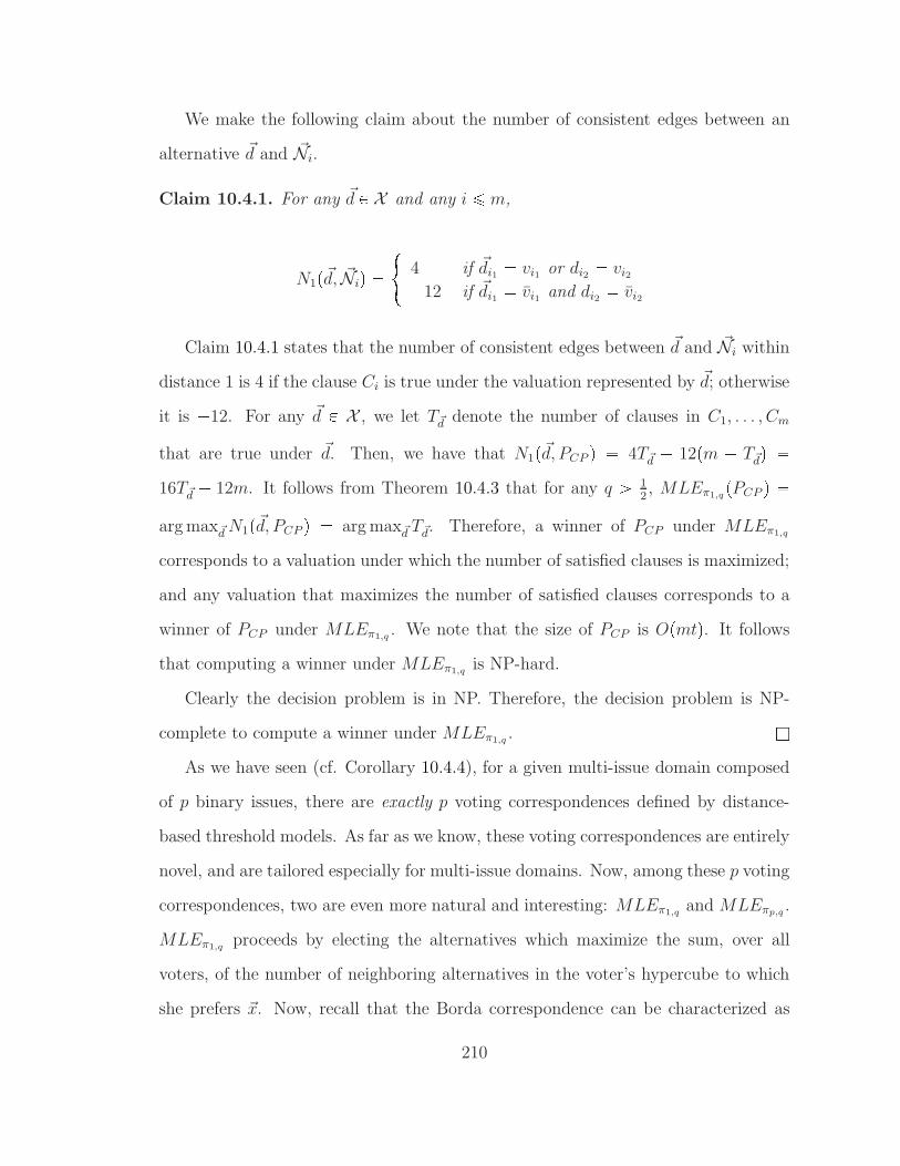
We make the following claim about the number of consistent edges between an
alternative ~d and ~Ni.
Claim 10.4.1. For any ~d P X and any i ¤ m,
N1p~d, ~Niq # 4 if ~di1 vi1 or di2 vi212 if ~di1 vi1 and di2 vi2
Claim 10.4.1 states that the number of consistent edges between ~d and ~Ni within
distance 1 is 4 if the clause Ci is true under the valuation represented by ~d; otherwise
it is 12. For any ~d P X , we let T~ddenote the number of clauses in C1, . . . , Cm
that are true under ~d. Then, we have that N1p~d, PCP q 4T~d 12pm T~d
q 16T~d
12m. It follows from Theorem 10.4.3 that for any q ¡ 12, MLEπ1,q
pPCP q arg max~d
N1p~d, PCP q arg max~dT~d
. Therefore, a winner of PCP under MLEπ1,q
corresponds to a valuation under which the number of satisfied clauses is maximized;
and any valuation that maximizes the number of satisfied clauses corresponds to a
winner of PCP under MLEπ1,q. We note that the size of PCP is Opmtq. It follows
that computing a winner under MLEπ1,qis NP-hard.
Clearly the decision problem is in NP. Therefore, the decision problem is NP-
complete to compute a winner under MLEπ1,q. l
As we have seen (cf. Corollary 10.4.4), for a given multi-issue domain composed
of p binary issues, there are exactly p voting correspondences defined by distance-
based threshold models. As far as we know, these voting correspondences are entirely
novel, and are tailored especially for multi-issue domains. Now, among these p voting
correspondences, two are even more natural and interesting: MLEπ1,qand MLEπp,q .
MLEπ1,qproceeds by electing the alternatives which maximize the sum, over all
voters, of the number of neighboring alternatives in the voter’s hypercube to which
she prefers ~x. Now, recall that the Borda correspondence can be characterized as
210
the correspondence where candidate x is a winner if it maximizes the sum, over all
voters, of the number of candidates the voter prefers to x. Therefore, MLEπ1,qis
somewhat reminiscent of Borda—except, of course, that we do not count all alter-
natives defeated by ~x but only defeated alternatives that are one of its neighbors in
the hypercube. MLEπp,q is even more intuitive: for each issue Xi, the winning value
maximizes the number of edges (summing over all voters) that are in favor of it, that
is, it is somewhat reminiscent of Kemeny.
So, MLEπ1,qand MLEπp,q are genuinely new voting correspondences for multi-
issue binary domains, which can be characterized in terms of maximum likelihood
estimators and are quite intuitive; lastly, MLEπp,q can be computed in polynomial
time. We conjecture that for any 2 ¤ k ¤ p 1, winner determination for MLEπk,q
is NP-hard.
10.5 Summary
In this chapter, we considered the maximum likelihood estimation (MLE) approach
to voting, and generalized it to multi-issue domains, assuming that the voters’ pref-
erences are expressed by CP-nets. We first studied whether issue-by-issue voting
rules and sequential voting rules can be represented by the MLE of some noise
model. For separable input profiles, we characterized MLEs of strongly/weakly
decomposable models as issue-by-issue voting correspondences composed of local
MLEWIVs/candidate scoring correspondences. Although we showed that no se-
quential voting correspondence can be represented as the MLE for a very weakly
decomposable model, we did obtain a positive result here under the assumption that
the number of voters is bounded above by a constant.
In the case where all issues are binary, we proposed a class of distance-based noise
models; then, we focused on a specific subclass of such models, parameterized by a
threshold. We identified the computational complexity of winner determination for
211

the two most relevant values of the threshold.
We note that, whereas Section 10.3 has a non-constructive flavor because we stud-
ied existing voting mechanisms and Theorem 10.3.3 is an impossibility theorem, quite
the opposite is the case for Section 10.4. Indeed, the MLE principle led us to define
genuinely new families of voting rules and correspondences for multi-issue domains.
These rules are radically different from the rules that had previously been proposed
and studied for these domains. Unlike sequential or issue-by-issue rules, they do not
require any domain restriction, and yet their computational complexity is not that
bad (the decision problem is NP-complete at worst, and sometimes polynomial in
the size of the CP-nets). We believe that these new rules are promising.
212
11
Strategic Sequential Voting
In previous two chapters we have been focusing on designing “good” voting rules
for combinatorial voting. In most of the previous work on combinatorial voting, it
was assumed that the voters report their true preferences using the voting language
we provide to them, when the voting language is expressive enough to do so. Now,
if the voters vote on issues sequentially, one issue after another according to some
ordering over issues, and are assumed to know the preferences of other voters well
enough, then we can expect them to vote strategically at each step, forecasting the
outcome at later steps conditional on the outcomes at earlier steps. Let us consider
the following motivating example (a similar example was shown in Lacy and Niou
(2000)).
Example 11.0.1. Three residents want to vote to decide whether they should build
a swimming pool and/or a tennis court. There are two issue S and T. S can take
the value of s (meaning “to build the swimming pool”) or s (meaning “not to build
the swimming pool”). Similarly, T takes a value in tt, tu. Suppose the preferences
of the three voters are, respectively, st ¡ st ¡ st ¡ st, st ¡ st ¡ st ¡ st and
213

st ¡ st ¡ st ¡ st. Voter 2 and 3 do not rank st as their first choices, because they
thought that the money could be spent on something else. Suppose the voters first
vote on issue S then on issue T. Since both issues are binary, the local rule used at
each step is majority (there will be no ties, because the number of voters is odd).
Voter 1 is likely to reason in the following way: if the outcome of the first step is
s, then voters 2 and 3 will vote for t, since they both prefer st to st, and the final
outcome will be st; but if the outcome of the first step is s, then voters 2 and 3 will
vote for t, and the final outcome will be st; because I prefer st to st, I am better off
voting for s, since either it will not make any difference, or it will lead to a final
outcome of st instead of st. If voters 2 and 3 reason in the same way, then 2 will
vote for s and 3 for s; hence, the result of the first step is s, and then, since two
voters out of three prefer st to st, the final outcome will be st. Note that the result
is fully determined, provided that (1) it is common knowledge that voters behave
strategically according to the principle we have stated informally, (2) the order in
which the issues are decided, as well as the local voting rules used in all steps, are also
common knowledge, and (3) voters’ preferences are common knowledge. Therefore,
these three assumptions allow the voters and the modeler (provided he knows as
much as the voters) to predict the final outcome.
Let us take a closer look at voter 1 in Example 11.0.1. Her preferences are
separable: she prefers s to s whatever the value of T is, and t to t whatever the
value of S is. And yet she strategically votes for s, because the outcome for S affects
the outcome for T. Moreover, while voters 2 and 3 have nonseparable preferences,
still, all three voters’ preferences enjoy the following property: their preferences over
the value of S are independent of the value of T. That is, the profile is pS ¡ Tq-legal. Hence, we can apply the sequential voting rule w.r.t. the order S ¡ T, using
majority rules for S and T. For the profile given in Example 11.0.1, the outcome of
214

the first step under the sequential voting rule will be s (since two voters out of three
prefer s to s, unconditionally), and the final outcome will be st. This outcome is
different from the outcome we obtain if voters behave strategically. The reason for
this discrepancy is that in Lang and Xia (2009), voters are not assumed to know the
others’ preferences and are assumed to vote truthfully.
We have seen that even if the voters’ preferences are O-legal, voters may in
fact have no incentive to vote truthfully. Consequently, existing results on multiple-
election paradoxes are not directly applicable to situations where voters vote strate-
gically.
Overview of this chapter
In this chapter, we analyze the complete-information game-theoretic model of se-
quential voting that we illustrated in Example 11.0.1. This model applies to any
preferences that the voters may have (not just O-legal ones), though they must be
strict orders on the set of all alternatives.
We focus on voting in multi-binary-issue domains, that is, for any i ¤ p, Xi
must take a value in t0i, 1iu. This has the advantage that for each issue, we can use
the majority rule as the local rule for that issue. We use a game-theoretic model
to analyze outcomes that result from sequential voting. Specifically, we model the
sequential voting process as a p-stage complete-information game as follows. There is
an order O over all issues (without loss of generality, let O X1 ¡ X2 ¡ ¡ Xp),
which indicates the order in which these issues will be voted on. For any 1 ¤ i ¤ p,
in stage i, the voters vote on issue Xi simultaneously, and the majority rule is used to
choose the winning value for Xi. We make the following game-theoretic assumptions:
it is common knowledge that all voters are perfectly rational; the order O and the
fact that in each step, the majority rule is used to determine the winner are common
knowledge; all voters’ preferences are common knowledge.
215

We can solve this game by a type of backward induction already illustrated in
Example 11.0.1: in the last (pth) stage, only two alternatives remain (corresponding
to the two possible settings of the last issue), so at this point it is a weakly dominant
strategy for each voter to vote for her more preferred alternative of the two. Then,
in the second-to-last (pp 1qth) stage, there are two possible local outcomes for thepp 1qth issue; for each of them, the voters can predict which alternative will finally
be chosen, because they can predict what will happen in the pth stage. Thus, thepp 1qth stage is effectively a majority election between two alternatives, and each
voter will vote for her more preferred alternative; etc. We call this procedure the
strategic sequential voting procedure (SSP).1
Given exogenously the order O over the issues, this game-theoretic analysis maps
every profile of strict ordinal preferences to a unique outcome. Since any function
from profiles of preferences to alternatives can be interpreted as a voting rule, the
voting rule that corresponds to SSP is denoted by SSPO.
Lacy and Niou (2000) showed that whenever there exists a Condorcet winner, it
must be the SSP winner. That is, SSP is Condorcet consistent. We will show that,
unfortunately, all three major types of multiple-election paradoxes (see Section 8.1)
also arise under SSP. To better present our results, we introduce a parameter which
we call the minimax satisfaction index (MSI). For an election with m alternatives
and n voters, it is defined in the following way. For each profile, consider the highest
position that the winner obtains across all input rankings of the alternatives (the
ranking where this position is obtained corresponds to the most-satisfied voter); this
is the maximum satisfaction index for this profile. Then, the minimax satisfaction
index is obtained by taking the minimum over all profiles of the maximum satisfaction
index. A low minimax satisfaction index means that there exists a profile in which
1 Lacy and Niou (2000) called such a procedure sophisticated voting following the conventionof Farquharson (1969).
216
the winner is ranked in low positions in all votes, thus indicating a multiple-election
paradox. Our main theorem is the following.
Theorem 11.3.1 For any p P N and any n ¥ 2p2 1, the minimax satisfaction
index of SSP when there are m 2p alternatives and n voters is tp22u. Moreover,
in the profile P that we use to prove the upper bound, the winner SSPOpP q is Pareto-
dominated by 2p pp 1qp2 alternatives.
We note that an alternative c Pareto-dominates another alternative c1 implies
that c beats c1 in their pairwise election. Therefore, Theorem 11.3.1 implies that the
winner for SSP is an almost Condorcet loser. It follows from this theorem that SSP
exhibits all three types of multiple-election paradoxes: the winner is ranked almost
in the bottom in every vote, the winner is an almost Condorcet loser, and the winner
is Pareto-dominated by almost every other alternative. We further show a paradox
(Theorem 11.3.6) that states that there exists a profile such that for any order O over
the issues, for every voter, the SSP winner w.r.t. O is ranked almost in the bottom
position. We also show that even when the voters’ preferences can be represented by
CP-nets that are compatible with a common order, multiple-election paradoxes still
arise.
Related work and discussion
The setting of SSP has been considered by Lacy and Niou (2000). But at a high
level, our motivation, results, and conclusion are quite different from those of Lacy
and Niou. We focus on the game-theoretic aspects of SSP, and we aim at examining
the equilibrium outcomes in voting games. They viewed SSP as a voting rule (see
Section 11.1.3 for more discussion on this point of view), and aimed at proposing
solutions to aggregate non-separable profiles in combinatorial voting. They showed
that SSP satisfies Condorcet consistency, but did not mention whether the other
types of multiple-election paradoxes can be avoided. We, on the other hand, show
217

that the other three types of multiple-election paradoxes still arise in SSP.2 In terms
of their conclusion, Lacy and Niou argued that SSP might not be a good solution
as a voting rule, because it requires the voters to have complete information about
the other voters’ true preferences. The paradoxes that will be shown in this chapter,
like the paradoxes we showed for Stackelberg voting games in Chapter 7, are an
ordinal version of price-of-anarchy results. Consequently, these paradoxes provide
more evidence that strategic behavior of the voters should be prevented, and therefore
motivate the study in the next chapter, where the objective is to design strategy-proof
voting rules that are computationally tractable for combinatorial domains.
More generally, SSP is closely related to multi-stage sophisticated voting, studied
by McKelvey and Niemi (1978), Moulin (1979), and Gretlei (1983). They investi-
gated the model where the backward induction outcomes correspond to the truthful
outcomes of voting trees. Therefore, SSP is a special case of multi-stage sophisti-
cated voting. However, their work focused on the characterization of the outcomes
as the outcomes in sophisticated voting (Farquharson, 1969), and therefore did not
shed much light on the quality of the equilibrium outcome. We, on the other hand,
are primarily interested in the strategic outcome of the natural procedure of voting
sequentially over multiple issues. Also, the relationship between sequential voting
and voting trees takes a particularly natural form in the context of domains with
multiple binary issues, as we will show. More importantly, we illustrate several
multiple-election paradoxes for SSP, indicating that the equilibrium outcome could
be extremely undesirable.
Another paper that is closely related to part of this work was written by
Dutta and Sen (1993). They showed that social choice rules corresponding to bi-
nary voting trees can be implemented via backward induction via a sequential vot-
2 In fact, those paradoxes were also discovered by Lacy and Niou in the same paper (Lacy andNiou, 2000), but they did not discuss whether they arise in SSP. See Section 8.1.
218

ing mechanism. This is closely related to the relationship revealed for multi-stage
sophisticated voting and will also be mentioned later in this chapter, that is, an
equivalence between the outcome of strategic behavior in sequential voting over mul-
tiple binary issues, and a particular type of voting tree. It should be pointed out
that the sequential mechanism that Dutta and Sen consider is somewhat different
from sequential voting as we consider it—in particular, in the Dutta-Sen mechanism,
one voter moves at a time, and a move consists not of a vote, but rather of choosing
the next player to move (or in some states, choosing the winner).
Nevertheless, the approach by Dutta and Sen and our approach are related at a
high level, though they are motivated quite differently: Dutta and Sen are interested
in social choice rules corresponding to voting trees, and are trying to create sequential
mechanisms that implement them via backward induction. We, on the other hand
again, are primarily interested in the strategic outcome of the natural mechanism for
voting sequentially over multiple issues, and use voting trees merely as a useful tool
for analyzing the outcome of this process.
11.1 Strategic Sequential Voting
11.1.1 Formal Definition
In this chapter, we focus on multi-binary-issue domains. That is, the multi-issue
domain is composed of multiple binary issues. Sequential voting on multi-binary-
issue domains can be seen as a game where in each step, the voters decide whether
to vote for or against the issue under consideration after reasoning about what will
happen next. We make the following assumptions.
1. All voters act strategically (in an optimal manner that will be explained later),
and this is common knowledge.
2. The order in which the issues will be voted upon, as well as the local voting rules
219

used at the different steps (namely, majority rules), are common knowledge.
3. All voters’ preferences on the set of alternatives are common knowledge.
Assumption 1 is standard in game theory. Assumption 2 merely means that
the rule has been announced. Assumption 3 (complete information) is the most
significant assumption. It may be interesting to consider more general settings with
incomplete information, resulting in a Bayesian game. Nevertheless, because the
complete-information setting is a special case of the incomplete-information setting
(where the prior distribution is degenerate), in that sense, all the worst-case negative
results obtained for the complete-information setting also apply to the incomplete-
information setting. That is, the restriction to complete information only strengthens
negative results. Of course, for incomplete information setting in general, we need a
more elaborate model to reason about voters’ strategic behavior.
Given these assumptions, the voting process can be modeled as a game that is
composed of p stages where in each stage, the voters vote simultaneously on one
issue. Let O be the order over the set of issues, which without loss of generality we
assume to be X1 ¡ ¡ Xp. Let P be the profile of preferences over X . The game
is defined as follows: for each i ¤ p, in stage i the voters vote simultaneously on
issue i; then, the value of Xi is determined by the majority rule (plus, in the case of
an even number of voters, some tie-breaking mechanism), and this local outcome is
broadcast to all voters.
We now show how to solve the game. Because of assumptions 1 to 3, at step i the
voters vote strategically, by recursively figuring out what the final outcome will be if
the local outcome for Xi is 0i, and what it will be if it is 1i. More concretely, suppose
that steps 1 to i1 resulted in issues X1, . . . , Xi1 taking the values d1, . . . , di1, and
let ~d pd1, . . . , di1q. Suppose also that if Xi takes the value 0i (respectively, 1i),
then, recursively, the remaining issues will take the tuple of values ~a (respectively,
220

~b). Then, Xi is determined by a pairwise comparison between p~d, 0i,~aq and p~d, 1i,~bqin the following way: if the majority of voters prefer p~d, 0i,~aq over p~d, 1i,~bq, then Xi
takes the value 0i; in the opposite case, Xi takes the value 1i. This process, which
corresponds to the strategic behavior in the sequential election, is what we call the
strategic sequential voting (SSP) procedure, and for any profile P , the winner with
respect to the order O is denoted by SSPOpP q.As we shall see later, SSP can not only be thought of as the strategic outcome of
sequential voting, but also as a voting rule in its own right. The following definition
and two propositions merely serve to make the game-theoretic solution concept that
we use precise; a reader who is not interested in this may safely skip them.
Definition 11.1.1. Consider a finite extensive-form game which transitions among
states. In each nonterminal state s, all players simultaneously take an action; this
joint local action profile pas1, . . . , a
snq determines the next state s1.3 Terminal states t
are associated with payoffs for the players (alternatively, players have ordinal pref-
erences over the terminal states). The current state is always common knowledge
among the players.4
Suppose that in every final nonterminal state s (that is, every state that has
only terminal states as successors), every player i has a (weakly) dominant action
asi . At each final nonterminal state, its local profile of dominant actions pas
1, . . . , asnq
results in a terminal state tpsq and associated payoffs. We then replace each final
nonterminal state s with the terminal state tpsq that its dominant-strategy profile
leads to. Furthermore suppose that in the resulting smaller tree, again, in every final
nonterminal state, every player has a (weakly) dominant strategy. Then, we can
repeat this procedure, etc. If we can repeat this all the way to the root of the tree,
3 In the extensive-form representation of the game, each state is associated with multiple nodes,because in the extensive form only one player can move at a node.
4 Hence, the only imperfect information in the extensive form of the game is due to simultaneousmoves within states.
221

then we say that the game is solvable by within-state dominant-strategy backward
induction (WSDSBI).
We note that the backward induction in perfect-information extensive-form games
is just the special case of WSDSBI where in each state only one player acts.
Proposition 11.1.2. If a game is solvable by WSDSBI, then the solution is unique.
Proposition 11.1.3. The complete-information sequential voting game with binary
issues (with majority as the local rule everywhere) is solvable by WSDSBI when voters
have strict preferences over the alternatives.
Both propositions are straightforward to prove and have been mentioned implic-
itly in Lacy and Niou (2000). We note that SSP corresponds to a particular balanced
voting tree, as illustrated in Figure 11.1 for the case p 3. In this voting tree, in the
first round, each alternative is paired up against the alternative that differs only on
the pth issue; each alternative that wins the first round is then paired up with the
unique other remaining alternative that differs only on the pp 1qth and possibly
the pth issue; etc. This bottom-up procedure corresponds exactly to the backward
induction (WSDSBI) process.
Of course, there are many voting trees that do not correspond to an SSP election;
this is easily seen by observing that there are only p! different SSP elections (cor-
responding to the different orders of the issues), but many more voting trees. The
voting tree corresponding to the order O X1 ¡ ¡ Xp is defined by the property
that for any node v whose depth is i (where the root has depth 1), the alternative
associated with any leaf in the left (respectively, right) subtree of v gives the value
0i (respectively, 1i) to Xi.
222

000 001 010 011 110 111101100
Figure 11.1: A voting tree that is equivalent to the strategic sequential votingprocedure (p 3). 000 is the abbreviation for 010203, etc.
11.1.2 Strategic Sequential Voting vs. Truthful Sequential Voting
We have seen on Example 11.0.1 that even when the profile P is O-legal, SSPOpP qcan be different from SeqOpMaj, . . . , MajqpP q. This means that even if the profile
is O-legal, voters may be better off voting strategically than truthfully. However,
SSPOpP q and SeqOpMaj, . . . , MajqpP q are guaranteed to coincide under the further
restriction that P is O-lexicographic.
Proposition 11.1.4. For any O-lexicographic profile P ,
SSPOpP q SeqOpMaj, . . . , MajqpP qThe intuition for Proposition 11.1.4 is as follows: if P is O-lexicographic, then,
as is shown in the proof of the proposition, when voters vote strategically under
sequential voting (the Seq process), they are best off voting according to their
true preferences in each round (their preferences in each round are well-defined
because voters have O-legal preferences in this case). When voters with O-legal
preferences vote truthfully in each round under sequential voting, the outcome is
SeqOpMaj, . . . , MajqpP q; when they vote strategically, the outcome is SSPOpP q;and so, these must be the same when preferences are O-lexicographic.
Now, there is another interesting domain restriction under which SSPOpP q and
SeqpMaj, . . . , MajqpP q coincide, namely when P is invpOq- legal, where invpOq 223

pXp ¡ . . . ¡ X1q.Proposition 11.1.5. Let invpOq Xp ¡ . . . ¡ X1. For any invpOq-legal profile P ,
SSPOpP q SeqinvpOqpMaj, . . . , MajqpP q.As a consequence, when P is separable, it is a fortiori invpOq-legal, and therefore,
SSPOpP q SeqinvpOqpMaj, . . . , MajqpP q, which in turn is equal to
SeqOpMaj, . . . , MajqpP q and coincides with issue-by-issue voting.
Corollary 11.1.6. If P is separable, then SSPOpP q SeqOpMaj, . . . , MajqpP q.11.1.3 A Second Interpretation of SSP
The first interpretation of SSP (that we follow in this chapter) is the one we have
discussed so far, namely, SSP consists in modeling sequential voting as a complete-
information game, which allows us to analyze sequential voting on multi-issue do-
mains from a game-theoretic point of view. For this, assumptions 1, 2, and 3 above
are crucial. Under this interpretation, SSPOpP q is a (specific kind of) equilibrium
for sequential voting.
However, there is a second interpretation of SSP. It consists in seeing SSPO
as a new voting rule on multi-issue domains (which is implementable in complete-
information contexts by using sequential voting).5 This seems to be the point of view
of Lacy and Niou (2000). This defines a family of voting rules (one for each order over
issues), which can be applied to any profile. The family of voting rules thus defined is
a distinguished subset of the family of voting trees. This interpretation does not say
anything about how preferences are to be elicited; unlike in the game-theoretic inter-
pretation, the p-step protocol does not apply here. The communication complexity
of finding the outcome of SSPO (without any complete-information assumption, of
5 Of course, by Gibbard-Satterthwaite (Gibbard, 1973; Satterthwaite, 1975), SSP is not strategy-proof.
224

course)6 is given as follows.
Proposition 11.1.7. When the voters’ preferences over alternatives are unrestricted,
the communication complexity of SSPO is Θp2p nq.Proof of Proposition 11.1.7: This now follows immediately from a result in
Conitzer and Sandholm (2005b), where it is established that the communication
complexity for balanced voting trees is Θpm nq for m alternatives and n voters.
Since we do not place any restrictions on the preferences in the multi-issue domain
in the statement of the proposition, the communication complexity is identical, and
m 2p. lThe upper bound in this proposition is obtained simply by eliciting the voters’
preferences for every pair of alternatives that face each other in the voting tree.
Now, Propositions 11.1.4 and 11.1.5 immediately give us conditions under which
this communication complexity can be reduced. Indeed, these Propositions say that
when P is O-lexicographic or invpOq-legal, then the SSP winner coincides with the
sequential election winner in the sense of Lang and Xia (2009). Now, the sequential
election winner in the sense of Lang and Xia (2009) can be found with Oppnq com-
munication, simply by having each agent vote for a value for the issue at each round.
This leads immediately to the following two corollaries (to Propositions 11.1.4 and
11.1.5, respectively).
Corollary 11.1.8. When the voters’ preferences over alternatives are O-lexicographic,
the communication complexity of SSPO is Oppnq.Corollary 11.1.9. When the voters’ preferences over alternatives are
invpOq-legal, the communication complexity of SSPO is Oppnq.6 The communication complexity of a voting rule is the smallest number of bits that must be trans-
mitted to compute the winner of that rule (i.e., taking the minimum across all correct protocols).See Conitzer and Sandholm (2005b).
225
11.1.4 The Winner is Sensitive to The Order over The Issues
In the definition of SSP, we simply fixed the order O to be X1 ¡ X2 ¡ ¡ Xp.
A question worth addressing is, to what extent is the outcome of SSP sensitive
to the variation of the order O? More precisely, given a profile P , let PWpP q |t~d P X | ~d SSPO1pP q for some order O1u|. PWpP q is the number of different
alternatives that can be made SSP winners by choosing a particular order O1. Then,
for a given number of binary issues p, we look for the maximal value of PWpP q, for
all profiles P on X D1 . . .Dp; we denote this number by MWppq.A first observation is that there are p! different choices for O1. Therefore, a trivial
upper bound on MWppq is p!. Since there are 2p alternatives, the p! upper bound
is only interesting when p! 2p, that is, p ¤ 3. Example 11.1.10 shows that when
p 2 or p 3, this trivial upper bound is actually tight, i.e. MWp2q 2! and
MWp3q 3!: there exists a profile such that by changing the order over the issues,
all p! different alternatives can be made winners. Due to McGarvey’s Theorem (see
Lemma 2.2.3), any complete and asymmetric directed graph G over the alternatives
corresponds to the majority graph of some profile (we recall that the majority graph
of a profile P is the directed graph whose vertices are the alternatives and containing
an edge from c to c1 if and only if a majority of voters in P prefer c to c1). Therefore,
in the example, we only show the majority graph instead of explicitly constructing
the whole profile.
Example 11.1.10. The majority graphs for p 2 and p 3 are shown in Fig-
ure 11.2. Let P (respectively, P 1) denote an arbitrary profile whose majority graph
is the same as Figure 11.2(a) (respectively, Figure 11.2(b)). It is not hard to verify
that SSPX1¡X2pP q 00 and SSPX2¡X1
pP q 01. For P 1, the value of SSPO1pP 1qfor the six possible orders is shown on Table 11.1. Note that 2! 2 and 3! 6. It
follows that when p 2 or p 3, there exists a profile for which the SSP winners
226
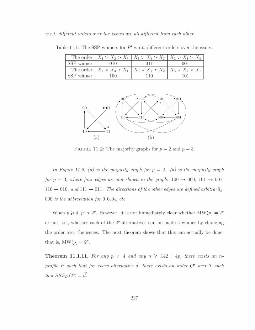
w.r.t. different orders over the issues are all different from each other.
Table 11.1: The SSP winners for P 1 w.r.t. different orders over the issues.
The order X1 ¡ X2 ¡ X3 X1 ¡ X3 ¡ X2 X2 ¡ X1 ¡ X3
SSP winner 010 011 001The order X2 ¡ X3 ¡ X1 X3 ¡ X1 ¡ X2 X3 ¡ X2 ¡ X1
SSP winner 100 110 101
00 01
10 11
000 001
010 011100 101
110 111
(a) (b)
Figure 11.2: The majority graphs for p 2 and p 3.
In Figure 11.2, (a) is the majority graph for p 2. (b) is the majority graph
for p 3, where four edges are not shown in the graph: 100 Ñ 000, 101 Ñ 001,
110Ñ 010, and 111Ñ 011. The directions of the other edges are defined arbitrarily.
000 is the abbreviation for 010203, etc.
When p ¥ 4, p! ¡ 2p. However, it is not immediately clear whether MWppq 2p
or not, i.e., whether each of the 2p alternatives can be made a winner by changing
the order over the issues. The next theorem shows that this can actually be done,
that is, MWppq 2p.
Theorem 11.1.11. For any p ¥ 4 and any n ¥ 142 4p, there exists an n-
profile P such that for every alternative ~d, there exists an order O1 over I such
that SSPO1pP q ~d.
227

Proof. We prove the theorem by induction on the number of issues p. Surprisingly,
the hardest part in the inductive proof is the base case: when we first show how to
construct a desirable majority graph M for p 4, then we show how to construct a
n-profile that corresponds to M.
To define M when p 4, we first define a majority graph M3 over X3 D2 D3D4. Let M1 denote the majority graph defined in Example 11.1.10 when p 3.
We note that M1 is defined over D1 D2 D3. The structure of M3 is exactly the
same as M1, except that M3 is defined over D2D3D4. Formally, let h1 : D1 Ñ D2
be a mapping such that h1p01q 02 and h1p11q 12; let h2 : D2 Ñ D3 be a mapping
such that h2p02q 03 and h2p12q 13; and let h3 : D3 Ñ D4 be a mapping such
that h3p03q 04 and h3p13q 14. Let h : D1 D2 D3 Ñ D2 D3 D4 be a
mapping such that for any pa2, a3, a4q P t0, 1u, hpa1, a2, a3q ph1pa1q, h2pa2q, h3pa3qq.For example, hp011203q 021304. Then, we let M3 hpM1q.
For any ~a pa2, a3, a4q P X3, let fp~aq p11,~aq and let gp~aq p01, a2, a3, a4q.That is, f concatenates 11 and ~a, and g flips the first two components of fp~aq. For
example, fp020304q 11020304 and gp020304q 11120304. We define M as follows.
(1) The subgraph of M over t11u X3 is fpM3q. That is, for any ~a,~b P X3, if
~a Ñ ~b in M1, then fp~aq Ñ fp~bq in M.
(2) The subgraph of M over t01u X3 is gpM3q.(3) For any ~a P X3, we have p11,~aq Ñ p01,~aq. For any ~a P X3 and ~a 111, we have
gp~aq Ñ fp~aq.(4) We then add the following edges to M. 0100 Ñ 1110, 1000 Ñ 0010, 1101 Ñ
0111, 0001 Ñ 1011, 1101 Ñ 0100, 1000 Ñ 0001, 0001 Ñ 1101, 0100 Ñ 1000,
1111 Ñ 0110, 1100 Ñ 0101, 0011 Ñ 1010, 1001 Ñ 0000, 1111 Ñ 0011,
0011Ñ 1100, 0011Ñ 1001, 1111Ñ 0000.
228

(5) Any other edge that is not defined above is defined arbitrarily.
Let P be an arbitrary profile whose majority graph satisfies conditions (1) through
(4) above. We make the following observations.
• If X1 is the first issue in O1, then the first component of SSPO1pP q is 11.
Moreover, every alternative whose first component is 11 (except 1111 and 1000)
can be made to win by changing the order of X2, X3, X4.
• If X1 is the last issue in O1, then the first component of SSPO1pP q is 01. More-
over, every alternative whose first component is 01 (except 0011 and 0100) can
be made to win by changing the order of X2, X3, X4.
• Let O1 X3 ¡ X1 ¡ X2 ¡ X4, we have SSPO1pP q 0100; let O1 X3 ¡ X1 ¡X4 ¡ X2, we have SSPO1pP q 1000; let O1 X4 ¡ X1 ¡ X3 ¡ X2, we have
SSPO1pP q 0011; let O1 X2 ¡ X4 ¡ X1 ¡ X3, we have SSPO1pP q 1111.
In summary, every alternative is a winner of SSP w.r.t. at least one order over the
issues. The reader can also check out the java program online at
http://www.cs.duke.edu/~lxia/Files/SSP.zip, to verify the correctness of such
a construction. We notice that conditions (1) through (4) impose 79 constraints on
pairwise comparisons. Therefore, using McGarvey’s trick (Lemma 2.2.3), for any
n ¥ 2 79 158, we can construct an n-profile whose majority graph satisfies
conditions (1) through (4). This means that the theorem holds for p 4.
Now, suppose that the theorem holds for p p1. Let P pV1, . . . , Vnq be an
n-profile over X 1 D2 . . . Dp11 such that n ¥ 142 4p1 and each alternative
in X 1 can be made to win in SSP by changing the order over X2, . . . , Xp11. Let
X D1 Dp11. Let f : X 1 Ñ X be the mapping defined as follows. For
any ~a P X 1, fp~aq p11,~aq. That is, for any ~a P X 1, f concatenates 11 and ~a. Let
g : X 1 Ñ X be the mapping defined as follows. For any ~a pa2, . . . , ap11q P X 1,229
gp~aq p01, a2, a3, . . . , ap11q. That is, for any ~a P X 1, g flips the first two components
of fp~aq. Next, we define an pn 4q-profile P 1 pV 11 , . . . , V
1n4q as follows.
For any i ¤ 2tpn 1q2u, we let V 1i "
fpViq ¡ gpViq if i is oddgpViq ¡ fpViq if i is even
. For any
2tpn 1q2u 1 ¤ i ¤ n, we let V 1i rfpViq ¡ gpViqs. For any j ¤ 4, we let
V 1nj $''&''% gp02 . . . 0p1q ¡ fp02 . . . 0p1q ¡ gp02 . . . 0p1p1q¡ fp02 . . . 0p1p1q ¡ gp12 . . . 1p1q ¡ fp12 . . . 1p1q if j is odd
gp12 . . . 1p1q ¡ fp12 . . . 1p1q ¡ gp12 . . . 1p0p1q¡ fp12 . . . 1p0p1q ¡ gp02 . . . 0p1q ¡ fp02 . . . 0p1q if j is even
For any pair of alternatives c, c1, and any profile P , we let DPpc, c1q denote the
number of times that c is preferred to c1, minus the number of times c1 is preferred
to c, both in the profile P . That is, DPpc, c1q ¡ 0 if and only if c beats c1 in their
pairwise election. We make the following observations on P 1.• For any ~a P X 1, DP 1pfp~aq, gp~aqq ¡ 0 and DP 1pp11,~aq, p01,~aqq ¡ 0.
• For any ~a,~b P X 1 (with ~a ~b), DP 1pfp~aq, fp~bqq ¡ 0 if and only if DP p~a,~bq ¡ 0;
DP 1pgp~aq, gp~bqq ¡ 0 if and only if DP p~a,~bq ¡ 0.
It follows that for any order O1 over tX2, . . . , Xp1u, we have SSPrX1¡O1spP 1q fpSSPO1pP qq (because after voting on issue X1, all alternatives whose first com-
ponent is 01 are eliminated, then it reduces to SSP over X 1); we also have that
SSPrO1¡X1spP 1q gpSSPO1pP qq (because in the last round, the two competing al-
ternatives are considering are fpSSPO1pP qq and gpSSPO1pP qq, and the majority of
voters prefer the latter). We recall that each alternative in X 1 can be made to win
w.r.t. an order O1 over tX2, . . . , Xp11u. It follows that each alternative in X can also
be made to win w.r.t. an order over tX1, . . . , Xp11u, which means that the theorem
holds for p p1 1. Therefore, the theorem holds for any p ¥ 4.
230
11.2 Minimax Satisfaction Index
In the rest of this chapter, we will show that strategic sequential voting on multi-
issue domains is prone to paradoxes that are almost as severe as previously studied
multiple-election paradoxes under models that are not game-theoretic (Brams et al.,
1998; Lacy and Niou, 2000).7 To facilitate the presentation of these results, we define
an index that is intended to measure one aspect of the quality of a voting rule, called
the minimax satisfaction index.
Definition 11.2.1. For any voting rule r, the minimax satisfaction index (MSI) of
r is defined as
MSIrpm, nq minPPLpX qn max
V PP m 1 rankV prpP qqwhere m is the number of alternatives, n is the number of voters, and rankV prpP qqis the position of rpP q in vote V .
We note that in this chapter m 2p, where p is the number of issues. The MSI
of a voting rule is not the final word on it. For example, the MSI for dictatorships is
m, the maximum possible value, which is not to say that dictatorships are desirable.
However, if the MSI of a voting rule is low, then this implies the existence of a paradox
for it, namely, a profile that results in a winner that makes all voters unhappy.
The third type of multiple-election paradoxes (see Section 8.1) implicitly refer
to such an index. We recall that the third type of multiple-election paradoxes state
that if voters vote on issues separately and optimistically, then there exists a profile
such that in each vote, the winner is ranked near the bottom; therefore this rule has
a very low MSI.
7 Even though Lacy and Niou (2000) have studied SSP, they actually did not examine whetherthere are any multiple-election paradoxes in SSP.
231

11.3 Multiple-Election Paradoxes for Strategic Sequential Voting
In this section, we show that over multi-binary-issue domains, for any natural number
n that is sufficiently large (we will specify the number in our theorems), there exists
an n-profile P such that SSPOpP q is ranked almost in the bottom position in each
vote in P . That is, the minimax satisfaction index is extremely low for the strategic
sequential voting procedure.
We first calculate the MSI for SSPO when the winner does not depend on the
tie-breaking mechanism. That is, either n is odd, or n is even and there is never a tie
in any stage of running the election sequentially. This is our main multiple-election
paradox result.
Theorem 11.3.1. For any p P N (p ¥ 2) and any n ¥ 2p2 1, MSISSPOpm, nq tp2 2u.8 Moreover, in the profile P that we use to prove the upper bound, the
winner SSPOpP q is Pareto-dominated by 2p pp 1qp2 alternatives.
Proof of Theorem 11.3.1: The upper bound on MSISSPOpm, nq is constructive,
that is, we explicitly construct a paradox.
For any n-profile P pV1, . . . , Vnq, we define the mapping fP : X Ñ Nn as
follows: for any c P X , fP pcq ph1, . . . , hnq such that for any i ¤ n, hi is the
number of alternatives that are ranked below c in Vi. For any l ¤ p, we denote
Xl Dl Dp and Ol Xl ¡ Xl1 ¡ ¡ Xp. For any vector ~h ph1, . . . , hnqand any l ¤ p, we say that ~h is realizable over Xl (through a balanced binary tree)
if there exists a profile Pl pV1, . . . , Vnq over Xl such that fPlpSSPOl
pPlqq ~h. We
first prove the following lemma.
8 If n is even, then to prove MSISSPO pm, nq ¥ tp2 2u, we restrict attention to profiles withoutties.
232

Lemma 11.3.2. For any l such that 1 ¤ l p,
~h p0, . . . , 0loomoontn2upl
, 1, . . . , 1loomoonpl1
, 2pl1 1, . . . , 2pl1 1looooooooooooooomooooooooooooooonrn2s1
qis realizable over Xl.
Proof of Lemma 11.3.2: We prove that there exists an n-profile Pl over Xl such
that SSPOlpPlq 1l 1p and ~h is realized by Pl. For any 1 ¤ i ¤ p l 1, we let
~bi 1l 1pi0p1i1p2i 1p. That is, ~bi is obtained from 1l 1p by flipping the
value of Xp1i. We obtain Pl pV1, . . . , Vnq in the following steps.
1. Let W1, . . . , Wn be null partial orders over Xl. That is, for any i ¤ n, the
preference relation Wi is empty.
2. For any j ¤ tn2u p l, we put 1l 1p in the bottom position in Wj ; we
put t~b1, . . . ,~bpl1u in the top positions in Wj.
3. For any j with tn2u 2 ¤ j ¤ n, we put 1l 1p in the top position of Wj ,
and we put t~b1, . . . ,~bpl1u in the positions directly below the top.
4. For j with tn2u p l 1 ¤ j ¤ tn2u 1, we define preferences as follows.
For any i ¤ p l 1, in Wtn2upli, we put ~bi in the bottom position, 1l 1p in
the second position from the bottom, and all the remaining bj (with j i) at the
very top.
5. Finally, we complete the profile arbitrarily: for any j ¤ n, we let Vj be an
arbitrary extension of Wj .
Let Pl pV1, . . . , Vnq. We note that for any i ¤ p l 1, ~bi beats any alternative
in Xlzt1l 1p,~b1, . . . ,~bpl1u in pairwise elections. Therefore, for any i ¤ p l 1,
the ith alternative that meets 1l 1p is ~bi, which loses to 1l 1p (just barely). It
follows that 1l 1p is the winner, and it is easy to check that fPlp1l 1pq ~h.
This completes the proof of the lemma. l233

Because the majority rule is anonymous, for any permutation π over 1, . . . , n and
any l p, if ph1, . . . , hnq is realizable over Xl, then phπp1q, . . . , hπpnqq is also realizable
over Xl. For any k P N, we define Hk t~h P t0, 1un :°
j¤n hj ¥ ku. That is, Hk is
composed of all n-dimensional binary vectors in each of which at least k components
are 1. We next show a lemma to derive a realizable vector over Xl1 from two
realizable vectors over Xl.
Lemma 11.3.3. Let l p, and let ~h1, ~h2 be vectors that are realizable over Xl. For
any ~h P Htn2u1, ~h1 p~h2 ~1q ~h is realizable over Xl1, where ~1 p1, . . . , 1q, and
for any ~a pa1, . . . , anq and any ~b pb1, . . . , bnq, we have ~a ~b pa1b1, . . . , anbnq.Proof of Lemma 11.3.3: Without loss of generality, we prove the lemma for
~h p0, . . . , 0loomoonrn2s1
, 1, . . . , 1loomoontn2u1
q. Let P1, P2 be two profiles over Xl, each of which is composed
of n votes, such that fpP1q ~h1 and fpP2q ~h2. Let P1 pV 11 , . . . , V 1
n q, P2 pV 21 , . . . , V 2
n q, ~a SSPOlpP1q, ~b SSPOl
pP2q. We define a profile P pV1, . . . , Vnqover Xl1 as follows.
1. Let W1, . . . , Wn be n null partial orders over Xl1.
2. For any j ¤ n and any ~e1, ~e2 P Xl, we let p1l1, ~e1q ¡Wjp1l1, ~e2q if ~e1 ¡V 1
j~e2;
and we let p0l1, ~e1q ¡Wjp0l1, ~e2q if ~e1 ¡V 2
j~e2.
3. For any rn2s ¤ j ¤ n, we let p1l1,~aq ¡Wjp0l1,~bq.
4. Finally, we complete the profile arbitrarily: for any j ¤ n, we let Vj be an
(arbitrary) extension of Wj such that p1l1,~aq is ranked as low as possible.
We note that p1l1,~aq is the winner of the subtree in which Xl1 1l1, p0l1,~bqis the winner of the subtree in which Xl1 0l1 , and p1l1,~aq beats p0l1,~bq in their
pairwise election (because the votes from rn2s to n rank p1l1,~aq above p0l1,~bq).Therefore, SSPOl1
pP q p1l1,~aq.234
Finally, we have that fP pp1l1,~aqq ~h1 p~h2 ~1q ~h. This is because p1l1,~aq is
ranked just as low as in the profile P1 for voters 1 through rn2s 1; for any voter j
with rn2s ¤ j ¤ n, additionally, p0l1,~bq needs to be placed below p1l1,~aq, which
implies that also, all the alternatives p0l1,~b1q for which j ranked ~b1 below ~b in P2
must be below p1l1,~aq in j’s new vote in P . This completes the proof of the lemma.lNow we are ready to prove the main part of the theorem. It suffices to prove that
for any n ¥ 2p2 1, there exists a vector ~hp P Nn such that each component of ~hp is
no more than tp2 1u, and ~hp is realizable over X . We first prove the theorem for
the case in which n is odd. We show the construction by induction in the proof of
the following lemma.
Lemma 11.3.4. Let n be odd. For any l1 p (such that l1 is odd),
~hl1 ptl12u, . . . , tl12uloooooooomoooooooonrn2spl121q2 , rl12s, . . . , rl12sloooooooomoooooooontn2upl121q2 qis realizable over Xpl11, and if l1 p, then
~hl11 ptl12u, . . . , tl12uloooooooomoooooooonl11
, rl12s, . . . , rl12sloooooooomoooooooonnpl15qpl11q2 , rl12s 1, . . . , rl12s 1loooooooooooooomoooooooooooooonpl13qpl11q2 q
is realizable over Xpl1.Proof of Lemma 11.3.4: The base case in which l1 1 corresponds to a single-
issue majority election over two alternatives, where rn2s 1 voters vote for one
alternative, and tn2u1 vote for the other, so that only the latter get their preferred
alternative.
Now, suppose the claim holds for some l1 ¤ p 2; we next show that the claim
also holds for l1 2. To this end, we apply Lemma 11.3.3 twice. Let l p l1 1.
First, let ~h p1, . . . , 1loomoonl1 , 2l1 1, . . . , 2l1 1loooooooooomoooooooooon
l11
, 0, . . . , 0loomoontn2ul11
, 2l1 1, . . . , 2l1 1loooooooooomoooooooooonrn2sl12
q235

By Lemma 11.3.2, ~h is realizable over Xl (via a permutation of the voters). Let
~h p1, . . . , 1loomoonl1 , 0, . . . , 0loomoon
l11
, 1, . . . , 1loomoontn2ul11
, 0, . . . , 0loomoonrn2sl12
q.Then, by Lemma 11.3.3, ~hl1 p~h ~1q ~h is realizable over Xl1. We have the
following calculation.
~hl1 p~h ~1q ~hprl12s 1, . . . , rl12s 1loooooooooooooomoooooooooooooonl1 ,tl12u, . . . , tl12uloooooooomoooooooon
l11
, rl12s, . . . , rl12sloooooooomoooooooonrn2spl13qpl11q2,rl12s 1, . . . , rl12s 1loooooooooooooomoooooooooooooonpl11q221
, rl12s, . . . , rl12sloooooooomoooooooontn2ul11
qThe partition of the set of voters into these five groups uses the fact that n ¥
2p2 1 implies rn2s pl1 3qpl1 1q2 ¥ 0. After permuting the voters in this
vector, we obtain the following vector which is realizable over Xl1:
~hl11 ptl12u, . . . , tl12uloooooooomoooooooonl11
, rl12s, . . . , rl12sloooooooomoooooooonnpl15qpl11q2 , rl12s 1, . . . , rl12s 1loooooooooooooomoooooooooooooonpl13qpl11q2 q
We next let ~h1 p1, . . . , 1loomoontn2u1
, 0, . . . , 0loomoonrn2s1
q and
~h1 p1, . . . , 1loomoonl11
, 0, . . . , 0loomoontn2ul1 , 2l11 1, . . . , 2l11 1looooooooooooomooooooooooooonrn2s1
qBy Lemma 11.3.2, the latter is realizable over Xl1. Thus, by Lemma 11.3.3, ~hl11p~h1~1q ~h1 is realizable over Xl2. Through a permutation over the voters, we obtain
the desired vector:
~hl12 ptl12u 1, . . . , tl12u 1loooooooooooooomoooooooooooooonrn2spl12qpl11q21
, rl12s 1, . . . , rl12s 1loooooooooooooomoooooooooooooontn2upl12qpl11q21
q236

which is realizable over Xl2. Therefore, the claim holds for l1 2. This completes
the proof of the lemma. lIf p is odd, from Lemma 11.3.4 we know that the theorem is true, by setting
l1 p. If p is even, then we first set l1 p 1; then, the maximum component of
~hl11 is rl12s 1 rpp 1q2s 1 p2 1. Thus we have proved the upper bound
in the theorem when n is odd.
When n is even, we have the following lemma (the proof is similar to the proof
of Lemma 11.3.4, so we omitted its proof).
Lemma 11.3.5. Let n be even. For any l1 p (such that l1 is odd),
~hl1 ptl12u, . . . , tl12uloooooooomoooooooonn2pl12l11q2 , rl12s, . . . , rl12sloooooooomoooooooon
n2pl12l11q2 qis realizable over Xpl11, and if l1 1 ¤ p, then
~hl11 ptl12u, . . . , tl12uloooooooomoooooooonl11
, rl12s, . . . , rl12sloooooooomoooooooonn1pl14qpl11q2 , rl12s 1, . . . , rl12s 1loooooooooooooomoooooooooooooonpl12qpl11q21
qis realizable over Xpl1.
The upper bound in the theorem when n is even follows from Lemma 11.3.5.
Moreover, we note that in the step from l1 to l1 1 (respectively, from l1 1 to
l1 2), no more than l1 new alternatives are ranked lower than the winner in the
profile that realizes ~hl11 (respectively, ~hl12). It follows that in the profile that
realizes ~hl11 (respectively, ~hl12) in Lemma 11.3.4 or Lemma 11.3.5, the number of
alternatives that are ranked lower than the winner by at least one voter is no more
than pl11ql12 l11 pl11qpl12q2 (respectively, pl12qpl13q2), which equalspp 1qp2 if l1 1 p (respectively, pp 1qp2 if l1 2 p). Therefore, in the profile
that we use to obtain the upper bound, the winner under SSPO is Pareto-dominated
by 2p pp 1qp2 alternatives.
237

Finally, we show that tp2 2u is a lower bound on MSISSPOpm, nq. Let P be
an n-profile; let SSPOpP q ~a, and let ~b1, . . . ,~bp be the alternatives that ~a defeats
in pairwise elections in rounds 1, . . . , p. It follows that in round j, more than half of
the voters prefer ~a to ~bj , because we assume that there are no ties in the election.
Therefore, summing over all votes, there are at least p ptn2u 1q occasions where
~a is preferred to one of ~b1, . . . ,~bp. It follows that there exists some V P P in which
~a is ranked higher than at least rp ptn2u 1qns ¥ tp2 1u of the alternatives
~b1, . . . ,~bp. Thus MSISSPOpm, nq ¥ tp2 2u.
(End of proof for Theorem 11.3.1.) lWe note that the number of alternatives is m 2p. Therefore, tp2 2u is
exponentially smaller than the number of alternatives, which means that there exists
a profile for which every voter ranks the winner very close to the bottom. Moreover,pp 1qp2 is still exponentially smaller than 2p, which means that the winner is
Pareto-dominated by almost every other alternative.
Naturally, we wish to avoid such paradoxes. One may wonder whether the para-
dox occurs only if the ordering of the issues is particularly unfortunate with respect
to the preferences of the voters. If not, then, for example, perhaps a good approach is
to randomly choose the ordering of the issues.9 Unfortunately, our next result shows
that we can construct a single profile that results in a paradox for all orderings of the
issues. While it works for all orders, the result is otherwise somewhat weaker than
Theorem 11.3.1: it does not show a Pareto-dominance result, it requires a number
of voters that is at least twice the number of alternatives, the upper bound shown
on the MSI is slightly higher than in Theorem 11.3.1, and unlike Theorem 11.3.1, no
matching lower bound is shown.
9 Of course, for any ordering of the issues, there exists a profile that results in the paradoxes inTheorem 11.3.1; but this does not directly imply that there exists a single profile that works for allorderings over the issues.
238

Theorem 11.3.6. For any p, n P N (with p ¥ 2 and n ¥ 2p1), there exists an
n-profile P such that for any order O over tX1, . . . , Xpu, SSPOpP q 11 1p, and
any V P P ranks 11 1p somewhere in the bottom p 2 positions.
Proof of Theorem 11.3.6: We first prove a lemma.
Lemma 11.3.7. For any c P X , X 1 X such that c R X 1, and any n P N (n ¥2m 2p1), there exists an n-profile that satisfies the following conditions. Let
F X zpX 1 Y tcuq. For any c1 P X 1, c defeats c1 in their pairwise election. For any c1 P X 1 and d P F , c1 defeats d in their pairwise election. For any V P P , c is ranked somewhere in the bottom |X 1| 2 positions.
Proof of Lemma 11.3.7: We let P pV1, . . . , Vnq be the profile defined as follows.
Let F1, . . . , Ftn2u1 be a partition of F such that for any j ¤ tn2u 1, |Fj| ¤r2mns 1. For any j ¤ tn2u 1, we let Vj rpF zFjq ¡ c ¡ X 1 ¡ Fjs. For anytn2u 2 ¤ j ¤ n, we let Vj rX 1 ¡ F ¡ cs. It is easy to check that P satisfies all
conditions in the lemma. lNow, let c 11 1p and X 1 t0112 1p, 110213 1p, . . . , 11 1p10pu. By
Lemma 11.3.7, there exists a profile P such that c beats any alternative in X 1 in
pairwise elections, any alternative in X 1 beats any alternative in X zpX 1 Y tcuq in
pairwise elections, and c is ranked somewhere in the bottom p 2 positions. This is
the profile that we will use to prove the paradox.
Without loss of generality , we assume that O X1 ¡ X2 ¡ ¡ Xp. (This is
without loss of generality because all issues have been treated symmetrically so far.) c
beats 11 1p10p in the first round; c will meet 11 1p20p11p in the next pairwise
election, because 11 1p20p11p beats every other alternative in that branch (they
are all in F ), and c will win; and so on. It follows that c SSPOpP q. Moreover, all
239

voters rank c in the bottom p 2 positions.
(End of proof for Theorem 11.3.6.) l11.4 Multiple-Election Paradoxes for SSP with Restrictions on Pref-
erences
The paradoxes exhibited so far placed no restriction on the voters’ preferences. While
SSP is perfectly well defined for any preferences that the voters may have over the
alternatives, we may yet wonder what happens if the voters’ preferences over al-
ternatives are restricted in a way that is natural with respect to the multi-issue
structure of the setting. In particular, we may wonder if paradoxes are avoided by
such restrictions. It is well known that natural restrictions on preferences sometimes
lead to much more positive results in social choice and mechanism design—for ex-
ample, single-peaked preferences allow for good strategy-proof mechanisms (Black,
1948; Moulin, 1980). In the next chapter we will see that we can characterize all
strategy-proof voting rules when the voters’ preferences are lexicographic, and their
local preferences over issues are restricted.
In this section, we study the MSI for SSPO for the following three cases: (1)
voters’ preferences are separable; (2) voters’ preferences are O-lexicographic; and
(3) voters’ preferences are O-legal. For case (1), we show a mild paradox (and
that this is effectively the strongest paradox that can be obtained); for case (2), we
show a positive result; for case (3), we show a paradox that is nearly as bad as the
unrestricted case.
Theorem 11.4.1. For any n ¥ 2p, when the profile is separable, the MSI for SSPO
is between 2rp2s and 2tp2u1.
That is, the MSI of SSPO when votes are separable is Θp?mq. We still have
that limmÑ8Θp?mqm 0, so in that sense this is still a paradox. However, its
240

convergence rate to 0 is much slower than for Θplog mqm, which corresponds to the
convergence rate for the earlier paradoxes.
Proof of Theorem 11.4.1: Let P pV1, . . . , Vnq. For any i ¤ p, we let di majpP |Xi
q. That is, di is the majority winner for the projection of the profile to
the ith issue. Because any separable profile is compatible with any order over the
issues, P is an O1-legal profile. It follows from Corollary 11.1.6 that SSPOpP q pd1, . . . , dpq. Without loss of generality pd1, . . . , dpq p11, . . . , 1pq.First, we prove the lower bound. Because for any i ¤ p, at least half of the voters
prefer 1i to 0i, the total number of times that a voter prefers 1 to 0 for an issue,
counted across all voters and issues, is at least p pn2q. Therefore, there exists j ¤ n
such that voter j prefers 1 to 0 on at least p2 issues, otherwise the total number of
times that a voter prefers 1 to 0 for an issue, counted across all voters and issues, is
no more than n pp2q 1 p pn2q, which is a contradiction. Formally put, there
exists j ¤ n such that |ti ¤ p : 1i ¡Vj0iu| ¥ p2. Without loss of generality for
every i ¤ rp2s, 1i ¡Vj0i. It follows that for any ~a P D1 Drp2s, we have thatp11, . . . , 1pq ¡Vj
p~a, 1rp2s1, . . . , 1pq. Therefore, the minimax satisfaction index is at
least 2rp2s.Next, we prove the upper bound. We first show that there exists a set of n
CP-nets N1, . . . ,Nn that satisfies the following two conditions.
1. For each j ¤ n, the number of issues on which Nj prefers 1 to 0 is exactlytp2u 1.
2. For each i ¤ p, majpN1|Xi, . . . ,Nn|Xi
q 1i.
The proof is by explicitly constructing the profile through the following n-step pro-
cess. Informally, we will allocate pptn2u 1q CPT entries “1 is preferred to 0”,tn2u 1 entries per issue, to n CP-nets as even as possible. Let k1 kp tn2u 1. In the jth step, we let Ij ti1, . . . , itp2u1u be the set of indices of the
241

highest k’s. Then, for any i P Ij , we let Nj|Xi r1i ¡ 0is and ki ki 1; for any
i R Ij , we let Nj|Xi r0i ¡ 1is. Because of the assumption that n ¥ 2p, we have
that nptp2u1q ¥ pptn2u1q, which means that after n steps, for all i ¤ p, ki ¤ 0.
It left to show that there exist extensions of N1, . . . ,Nn such that in each of these
extensions, 11 1p is ranked within bottom 2tp2u1 positions. To show this, we use
the following lemma.
Lemma 11.4.2. For any partial order W and any alternative c, we let |DownW pcq| tc1 : c ©W c1u, that is, |DownW pcq| is the set of all alternatives (including c) that are
less preferred to c in W . There exists a linear order V such that V extends W and
c is ranked in the |DownW pcq|th position from the bottom.
The proof of Lemma 11.4.2 is quite straightforward: for every alternative d such
that d R DownW pcq, we put d ¡ c in the partial order. This does not violate
transitivity, which means that the ordering relation obtained in this way is a partial
order, denoted by W 1. Then, let V be an arbitrary linear order that extends W 1. It
follows that c is ranked at the DownW pcqth position from the bottom in V .
We note that for any j ¤ n, the number of entries in Nj where 1 ¡ 0 is no
more than tp2 1u. Therefore, for any j ¤ n, |Down¡Njp11 1pq| ¤ 2tp21u (we
recall that ¡Njis the partial order that Nj encodes). Let V1, . . . , Vn be extensions
of N1, . . . ,Nn, respectively, where for all j ¤ n, 11 1p is ranked as low as possible
in any Vj. It follows from Lemma 11.4.2 that for any j ¤ n, 11 1p is ranked in the
2tp21uth position from the bottom in Vj. This proves the upper bound.
(End of proof for Theorem 11.4.1.) lTheorem 11.4.3. For any p P N (p ¥ 2) and any n ¥ 5, when the profile is O-
lexicographic, MSIpSSPOq 3 2p2 1. Moreover, SSPOpP q is ranked somewhere
in the top 2p1 positions in at least n2 votes.
242

Naturally limmÑ8p3m41qm 34, so in that sense there is no paradox when
votes are O-lexicographic.
Proof of Theorem 11.4.3: The proof is for profiles without ties. The other cases
can be proved similarly. Without loss of generality SSPOpP q 11 1p and for
every j ¤ tn2u1, 11 ¡Vj |X101. It follows that in V1, . . . , Vtn2u1, 11 1p is ranked
within top 2p1 m2 positions. Because in at least tn2u 1 votes 11 : 12 ¡ 02,
there exists a vote V P P such that 11 ¡V |X101 and 11 : 12 ¡V |X2:11
02. It follows
that 11 1p is ranked in the p3 2p2 1qth position from the bottom. This proves
that when the profile is O-lexicographic, MSIpSSPOq ¥ 3 2p2 1.
We next prove that 3 2p2 1 is also an upper bound. Consider the profile
P pV1, . . . , Vnq defined as follows. For any j ¤ tn2u 1, 11 ¡Vj |X101; for anytn2u 2 ¤ j ¤ n, 12 ¡Vj |X2:11
02; for j 1, 2, 12 ¡Vj |X2:1102; for any 3 ¤ j ¤ n and
any 3 ¤ i ¤ p, 1i ¡Vj |Xi:111i10j; for any local preferences of any voter that is not
defined above, let 0 be preferred to 1.
We note that for any i ¤ p, more than n2 votes in P |Xi:111i1prefer 1i to 0i,
which means that SSPOpP q 11 1p. It is easy to check that in any vote, 11 1p
is ranked somewhere within the bottom 3 2p2 1 positions.
(End of proof for Theorem 11.4.3.) lUnder the previous two restrictions (separability and O-lexicographicity), SSPO
coincides with SeqpMaj, . . . , Majq (by Corollary 11.1.6 and Proposition 11.1.4, re-
spectively). Therefore, Theorems 11.4.1 and 11.4.3 also apply to sequential voting
rules as well as issue-by-issue voting rules.
Finally, we study the MSI for SSPO when the profile is O-legal. Theorem 11.4.6
shows that it is nearly as bad as the unrestricted case (Theorem 11.3.1). The proof
of Theorem 11.4.6 is the most involved proof in this chapter. The idea of the
proof is similar to that of the proof for Theorem 11.3.1, but now we cannot ap-
243

ply Lemma 11.3.3, because O-legality must be preserved. We start with a simpler
result that shows the idea of the construction.
Theorem 11.4.4. There exists a way to break ties in SSPO such that the following
is true. Let SSP 1O be the rule corresponding to SSPO plus the tiebreaking mechanism.
For any p P N, there exists an O-legal profile that consists of two votes, such that
in one of the two votes, no more than rp2s alternatives are ranked lower than the
winner SSP 1OpP q; and in the other vote, no more than tp2u alternatives are ranked
lower than SSP 1OpP q.Proof of Theorem 11.4.4: The proof is by induction on p. When p 2, let
the CPT of N1 be 01 ¡ 11, 01 : 12 ¡ 02, 11 : 12 ¡ 02; let the CPT of N2 be
11 ¡ 01, 01 : 02 ¡ 12, 11 : 02 ¡ 12; V1 r0112 ¡ 0102 ¡ 1112 ¡ 1102s; V2 r1102 ¡0102 ¡ 1112 ¡ 0112s. In the first step, ties are broken in favor of 1112. Given 11, ties
are broken in favor of 12; given 01, ties are broken in favor of 12.
Suppose the claim is true for p l. Next we construct N1 and N2 for p l 1.
Let N 11, N
12, V 1
1 , V 12 be the CP-nets and the votes for the case of p l, where the multi-
issue domain is D2 Dl1. Without loss of generality |DownV1p12 1l1q| ¤rl2s and |DownV2
p12 1l1q| ¤ tl2u. We recall that for any vote V and any al-
ternative c, DownV pcq (defined in Lemma 11.4.2) is the set of all alternatives that
are ranked below c in V , including c. Let ~e P D2 Dl1 be an arbitrary
alternative such that 12 1l1 ¡V2~e. Such an ~e always exists, because if on the
contrary 12 1l1 is in the bottom of V2, it must be ranked higher than at least l
other alternatives in V1 to win the election, which contradicts the assumption that|DownV1p12 1l1q| ¤ rl2s. We will explain later why we choose ~e in such a way.
Let N 1 (respectively, N
2 ) be the separable CP-net (we recall that a CP-net
is separable if its graph has no edges) D2 Dl1 in which ~e is in the top
(respectively, bottom) position. For i 1, 2, we let Ni be a CP-net over D1 244

Dl1, defined as follows:
• 01 ¡Ni11.
• The sub-CP-net of Ni restricted on X1 11 is N 1i ;
• The sub-CP-net of Ni restricted on X1 01 is N i ;
Let V1, V2 be the extension of N1 and N2 respectively, that satisfy the following
conditions:
• For any ~b, ~d P D2 Dl1 such that ~b ~e, and any i 1, 2, we havep01,~bq ¡Vip11, ~dq. This condition can be satisfied, because we have 01 ¡Ni
11.
• For any ~b, ~d P D2 Dl1, and any i 1, 2, we have that p11,~bq ¡Vip11, ~dq
if and only if ~b ¡V 1i
~d. This condition says that if we focus on the order of the
alternatives whose X1 component is 11 in Vi, then it is the same as in V 1i .
• For any ~d P D2 Dl1, we have that p01, ~eq ¡V1p11, ~dq.
• p11, . . . , 1l1q ¡V2p01, ~eq ¡V2
p11, ~eq.We let the tie-breaking mechanism be defined as follows: in the first step, ties are
broken in favor of 11; in the subgame in which X1 11, ties are broken in the same
way as for the profile pV 11 , V
12q (such that 12 1l1 is the winner for the profile); in
the subgame in which X1 01, ties are broken in such a way that ~e is the winner
(because ~e is ranked in the top position in one vote, and in the bottom position in
the other, there exists a tie-breaking mechanism under which ~e is the winner).
We note that 11 1p ¡V1
~d if and only if ~d p11, ~d1q for some ~d1 P D2 Dl1
such that 12 1p ¡V 11
~d1. It follows that |DownV1p11 1l1q| |DownV 1
1p12 1l1q|.
We also note that 11 1l1 ¡V2
~b if and only if ~b p01, ~eq or ~b p11,~b1q for some
245

~b1 P D2 Dl1 such that 12 1p ¡V 12
~b1. It follows that |DownV2p11 1l1q| |DownV 1
2p12 1l1q| 1. Therefore, we have the following inequalities.|DownV1
p11 1l1q| ¤ tpl 1q2u|DownV2p11 1pq| ¤ tl2u 1 ¤ rpl 1q2s
Here the trick to choose ~e such that 12 1l1 ¡V 12
~e is crucial, because we force
01 ¡N211 and 11 1l1 ¡V2
p01, ~eq, which implies that 11 1l1 ¡V2p01, ~eq ¡V2p11, ~eq (since V2 extends N2). If we chose ~e such that ~e ¡V 1
212 1l1, then we would
have that |DownV2p11 1l1q| |DownV 1
2p12 1l1q| 2, which does not prove the
claim for p l 1.
Next, we verify that SSPOpV1, V2q 11 1l1. We note that p01, ~eq ¡V111 1l1.
Therefore, in the first step voter 1 will vote for 01. Meanwhile, 11 1l1 ¡V2p01, ~eq,
which means that in the first step voter 2 will vote for 11. Because ties are broken
in favor of 11 in the first step, we will fix X1 11. Then, in the following steps (step
2, . . . , l 1), 12, . . . , 1l1 will be the winners by induction hypothesis, which means
that SSPOpV1, V2q 11 1l1.
Therefore, the claim is true for p l 1. This means that the claim is true for
any p P N.
Example 11.4.5. Let us show an example of the above construction from p 2 to
p 3. In N1, we have 01 ¡ 11, 11 : N 1 , and 01 : N 1
1, where N 11 is 02 ¡ 12, 02 : 13 ¡
03, 12 : 13 ¡ 03. (We note that N 11 is defined over D2 D3.) V1 restricted to 11 is
V 11 r0213 ¡ 0203 ¡ 1213 ¡ 1203s (which is, again, over D2 D3). Let ~e 0213.
Therefore, we have the following construction:
V1 010213 ¡ 011213 ¡ 010203 ¡ 011203 ¡ 110213 ¡ 110203 ¡ 111213 ¡ 111203
V2 011203 ¡ 010203 ¡ 011213 ¡ 111203 ¡ 110203 ¡ 111213 ¡ 010213 ¡ 110213
Ties are broken in a way such that if we are in the branch in which X1 11,
then 1213 is the winner; and if we are in the branch in which X1 01, then ~e 0213
246
is the winner. In the first step, ties are broken in favor of 11. Then, the sub-game
winners are 111213 and 010213. Since exactly one vote (V1) prefers 010213 to 111213,
and the other vote V2 prefers 111213 to 010213, the winner is 111213.
(End of proof for Theorem 11.4.4.) lWe emphasize that, unlike any of our other results, Theorem 11.4.4 is based on
a specific tie-breaking mechanism. The next theorem concerns the more general and
complicated case in which n can be either odd or even, and the winner does not
depend on the tie-breaking mechanism. That is, there are no ties in the election.
The situation is almost the same as in Theorem 11.3.1.
Theorem 11.4.6. For any p, n P N with n ¥ 2p2 2p 1, there exists an O-
legal profile such that in each vote, no more than rp2s 4 alternatives are ranked
lower than SSPOpP q. Moreover, SSPOpP q is Pareto-dominated by at least 2p 4p2
alternatives.
Of course, the lower bound on the MSI from Theorem 11.3.1 still applies when
the profile is O-legal, so together with Theorem 11.4.6 this proves that the MSI for
SSPO when the profile is O-legal is Θplog mq, just as in the unrestricted case.
Proof of Theorem 11.4.6: For simplicity, we prove the theorem for the case
in which n 2p2 2p 1. The proof for the case in which n ¡ 2p2 2p 1
is similar. For any l ¤ p, we let Xl t0l, 1lu t0l1, 1l1u t0p, 1pu; let
Ol Xl ¡ Xl1 ¡ ¡ Xp. We first prove the following claim by induction.
Claim 11.4.1. For any l ¤ p, there exists a Ol-legal profile Pl Al Y Bl Y Al YBl Y tclu over Xl, where Al tal
1, . . . , alp2u, Bl tbl
1, . . . , blp2u, Al tal
1, . . . , alpu,
Bl tbl1, . . . , b
lpu, that satisfies the following conditions.
• SSPOlpPlq 1l 1p.
• For any V P Pl, |DownV p1l 1pq| ¤ rpp l 1q2s 5.
247
• For any pplqp ¤ j ¤ p2, |Downaljp1l 1pq| ¤ rppl1q2s3, |Downbl
jp1l 1pq| ¤rpp l 1q2s 3.
• For any pl ¤ j ¤ p, |Downaljp1l 1pq| ¤ rppl1q2s3, |Downbl
jp1l 1pq| ¤rpp l 1q2s 3.
• If p l 1 is odd, then
– for any VB P B, |DownVBp1l 1pq| ¤ rpp l 1q2s 4;
– for any pp lqp ¤ j ¤ p2, |Downbljp1l 1pq| ¤ rpp l 1q2s 2;
– and for any p l ¤ j ¤ p, |Downbljp1l 1pq| ¤ rpp l 1q2s 2.
• 1l 1p is ranked higher than 1l 1p20p10p in all votes in Pl.
Proof of Claim 11.4.1: We prove the claim by induction on l. When l p1, we
let all votes in Pp1 be 1p11p ¡ 1p10p ¡ 0p11p ¡ 0p10p. It is easy to check that
Pp1 satisfies all the conditions in the claim. Suppose the claim is true for l ¤ p, we
next prove that the claim is also true for l 1. We show the existence of Pl1 by
construction for the following two cases.
Case 1: p l 1 is even.
We let N l1, . . . ,N
lpl1,N
lA,N l
B be separable CP-nets over Xl, defined as follows.
• Let 1l 1p20p10p be in the bottom position of N lA; let 1l 1p20p10p be in
the top position of N lB.
• For any 1 ¤ i ¤ p l 1, let 1l 1li20li11li 1p20p10p be in the
top position of N li ; let 1l 1p21p10p be in the top position of N l
pl; let
1l 1p20p11p be in the top position of N lpl1.
For any linear order V over Xl, we let the composition of V and N (where N PtN l1, . . . ,N
lpl1,N
lA,N l
Bu) be a partial order Ol1 over Xl1, defined as follows.
248

• The restriction of Ol1 on Xl1 1l1 is V . That is, for any ~d1, ~d2 P Xl such
that ~d1 ¡V~d2, we let p1l1, ~d1q ¡Ol1 p1l1, ~d2q.
• The restriction of Ol1 on Xl1 0l1 is the partial order encoded by N . That
is, for any ~d1, ~d2 P Xl such that ~d1 ¡N~d2, we let p0l1, ~d1q ¡Ol1 p0l1, ~d2q.
• For any ~d P Xl, we let p0l1, ~dq ¡Ol1 p1l1, ~dq.• If N P tN l
1, . . . ,Nlpl1,N
lAu, we let 1l11l 1p ¡Ol1 0l11l 1p20p10p.
We are now ready to define Pl1. Any V P Pl1 has a counterpart in Pl. For
example, the counterpart of al11 is al
1. For any V P Pl1, V is defined to be the
extension of the composition of V ’s counterpart in Pl and some N (where N PtN l1, . . . ,N
lpl1,N
lA,N l
Bu), in which 1l1 1p is ranked as low as possible. Next we
specify which N that each V P Pl1 corresponds to in the following table.
Table 11.2: From Pl to Pl1.
for all votes in Pl1 is composed of
1 ¤ j ¤ p al1j al
j N lA
j ¤ pp lqp al1j al
j N lApp lqp 1 ¤ j ¤ pp l 1qp al1
j alj N l
jpplqppp l 1qp 1 ¤ j ¤ p2 al1j al
j N lA
bl1pl2 bl
pl2 N lA
j p l 2 bl1j bl
j N lB
j ¤ p2 bl1j bl
j N lB
cl1 cl N lB
It follows that Pl1 is Ol1-legal. By Lemma 11.4.2, we have the following calcu-
lation.
• For any 1 ¤ j ¤ p, |Downal1
jp1l1 1pq| |Downal
jp1l 1pq| 1. This is
because for any ~d P Xl such that ~d P Downaljp1l 1pq, 1l1 1p is ranked
249

higher than p1l1, ~dq in al1j ; and moreover, 1l1 1p is ranked higher than
0l11l 1p20p10p in al1j .
• For any 1 ¤ j ¤ p, |Downal1pplqpjp1l1 1pq| |Downalpplqpj
p1l 1pq| 3.
This is because for any ~d P Xl such that ~d P Downapplqpjp1l 1pq, 1l1 1p
is ranked higher than p1l1, ~dq in applqpj; and moreover, 1l1 1p is ranked
higher than 0l11l 1p20p10p in applqpj.
• For any j ¤ pp lqp or pp l 1qp 1 ¤ j ¤ p2, |Downal1
jp1l1 1pq| |Downal
jp1l 1pq| 1.
• |Downbl1
pl2
p1l1 1pq| |Downblpl2
p1l 1pq| 1.
• For any VB P pBl1 Y Bl1 Y tcuqztbpl2u,|DownVBp1l1 1pq| |DownV l
Bp1l 1pq|,
where V lB is the counterpart of VB in Pl.
We next prove that SSPOl1pPl1q 1l1 lp. We note that Pl1|Xl11l1
Pl.
Therefore, if in the first step 1l1 is chosen, then the winner is 1l1 1p. We also
note that Pl1|Xl10l1is separable (and the CP-nets are N l
1, . . . ,Nlpl1, p2 p
copies of N lA and p2 p copies of N l
B). Therefore, if in the first step 0l1 is
chosen, then the winner is 0l11l 1p21p11p. Because exactly p2 p 1 votes
in Pl1 prefer 0l11l 1p21p11p to 1l1 1p (those votes corresponds to N lB in
the construction), we have that 1l1 is the winner in the first step. Therefore,
SSPOl1pPl1q 1l1 lp. It is also easy to verify that Pl1 satisfies all condi-
tions in the claim.
Case 2: p l1 is odd. The construction is similar as in the even case. The only
difference is that we switch the role of Al and Bl (also Al and Bl). l250
The theorem follows from Claim 11.4.1 by letting l 1, and it is easy to check
that in P1 in Claim 11.4.1 (l 1), no more than 4p2 alternatives have been ranked
lower than SSPOpP1q in any vote, which means that SSPOpP1q is Pareto-dominated
by at least 2p 4p2 alternatives.
(End of proof for Theorem 11.4.6.) l11.5 Summary
In this chapter, we considered a complete-information game-theoretic analysis of se-
quential voting on binary issues, which we called strategic sequential voting. Specifi-
cally, given that voters have complete information about each other’s preferences and
their preferences are strict, the game can be solved by a natural backward induction
process (WSDSBI), which leads to a unique solution. We showed that under some
conditions on the preferences, this process leads to the same outcome as the truthful
sequential voting, but in general it can result in very different outcomes. We ana-
lyzed the effect of changing the order over the issues that voters vote on and showed
that, in some elections, every alternative can be made a winner by voting according
to an appropriate order over the issues.
Most significantly, we showed that strategic sequential voting is prone to multiple-
election paradoxes; to do so, we introduced a concept called minimax satisfaction
index, which measures the degree to which at least one voter is made happy by the
outcome of the election. We showed that the minimax satisfaction index for strategic
sequential voting is exponentially small, which means that there exists a profile for
which the winner is ranked almost in the bottom positions in all votes; even worse,
the winner is Pareto-dominated by almost every other alternative. We showed that
changing the order of the issues in sequential voting cannot completely avoid the
paradoxes. These negative results indicate that the solution of the sequential game
can be extremely undesirable for every voter. We also showed that multiple-election
251

paradoxes can be avoided to some extent by restricting voters’ preferences to be
separable or lexicographic, but the paradoxes still exist when the voters’ preferences
are O-legal.
252

12
Strategy-Proof Voting Rules over Restricted
Domains
We have seen in Chapter 7 and Chapter 11 that in some voting games, strategic
behavior sometimes leads to extremely undesirable outcomes. Therefore, we may
want to prevent voters’ strategic behavior. However, the Gibbard-Satterthwaite the-
orem tells us that for any voting rule that satisfies some natural properties, there
must exist at least one voter who has an incentive to misreport her preferences, if
the voters are allowed to use any linear order to represent their preferences. To
circumvent the Gibbard-Satterthwaite theorem, researchers in Computational So-
cial Choice have investigated the possibility of using computational complexity to
prevent voters’ strategic behavior. Chapter 4 showed that for some common vot-
ing rules computational complexity can provide some protection from manipulation,
while Chapter 5 gave some evidence that computational complexity does not seem
to be a very strong barrier against manipulation.
In fact, there is another, older, line of research on circumventing the Gibbard-
Satterthwaite theorem. This line, which has been pursued mainly by economists, is
to restrict the domain of preferences. That is, we assume that voters’ preferences
253

always lie in a restricted class. An example of such a class is that of single-peaked
preferences (Black, 1948). For single-peaked preferences, desirable strategy-proof
rules exist, such as the median rule. Other strategy-proof rules are also possible in
this preference domain: for example, it is possible to add some artificial (phantom)
votes before running the median rule. In fact, this characterizes all strategy-proof
rules for single-peaked preferences (Moulin, 1980). On the other hand, preferences
have to be significantly restricted to obtain such positive results: Aswal et al. (2003)
extend the Gibbard-Satterthwaite theorem, showing that if the preference domain is
linked, then with three or more alternatives the only strategy-proof voting rule that
satisfies non-imposition is a dictatorship.
In this chapter we will focus on exploring the possibility of using domain restric-
tion to circumvent the Gibbard-Satterthwaite theorem in multi-issue domains. The
problem of characterizing strategy-proof voting rules in multi-issue domains has al-
ready received significant attention. Strategy-proof voting rules for high-dimensional
single-peaked preferences (where each dimension can be seen as an issue) have been
characterized (Border and Jordan, 1983; Barbera et al., 1993, 1997; Nehring and
Puppe, 2007). Barbera et al. (1991) characterized strategy-proof voting rules when
the voters’ preferences are separable, and each issue is binary (that is, the domain for
each issue has two elements). Ju (2003) studied multi-issue domains where each issue
can take three values: “good”, “bad”, and “null”, and characterized all strategy-proof
voting rules that satisfy null-independence, that is, if a voter votes “null” on an issue
i, then her preferences over other issues do not affect the value of issue i.
The prior research that is closest to ours was performed by Le Breton and Sen
(1999). They proved that if the voters’ preferences are separable, and the restricted
preference domain of the voters satisfies a richness condition, then, a voting rule is
strategy-proof if and only if it is an issue-by-issue voting rule, in which each issue-wise
voting rule is strategy-proof over its respective domain.
254

Despite its elegance, the work by Le Breton and Sen is limited by the restrictive-
ness of separable preferences: as we have argued in Chapter 8, in general, a voter’s
preferences on one issue depend on the decision taken on other issues. On the other
hand, one would not necessarily expect the preferences for one issue to depend on
every other issue. Therefore, it seems that sequential voting (Section 8.3) is better
than issue-by-issue voting. While the assumption of sequential voting that there
exists an ordering O over issues such that all voters’ preferences are O-legal is still
restrictive, it is much less restrictive than assuming that preferences are separable.
Chapter 9 and Chapter 10 concerned how to design new voting rules when voters
use a much more expressive voting language (i.e., possibly cyclic CP-nets), but in
this chapter, we only study the setting where all voters’ preferences are O-legal, and
w.l.o.g. we fix O X1 ¡ X2 ¡ ¡ Xp.
The main theorem of this chapter is the following: over lexicographic preference
domains (where earlier issues dominate later issues in terms of importance to the
voters), the class of strategy-proof voting rules that satisfy non-imposition is exactly
the class of voting rules that can be decomposed into multiple strategy-proof local
rules, one for each issue and each setting of the issues preceding it. Technically, it is
exactly the class of all conditional rule nets (CR-nets), defined later in this chapter
but analogous to CP-nets, whose local (issue-wise) entries are strategy-proof voting
rules. CR-nets represent how the voting rule’s behavior on one issue depends on the
decisions made on all issues preceding it. Conceptually, this is similar to how acyclic
CP-nets represent how a voter’s preferences on one issue depend on the decisions
made on all issues preceding it.
12.1 Conditional Rule Nets (CR-Nets)
In this section, we give the motivation and formal definition of CR-nets. In a se-
quential voting rule, the local voting rule that is used for a given issue is always the
255

same, that is, the local voting rule does not depend on the decisions made on earlier
issues (though, of course, the voters’ preferences for this issue do depend on those
decisions).
However, in many cases, it makes sense to let the local voting rules depend on
the values of preceding issues. For example, let us consider again the setting in
Example 8.0.2, where a group of people must make a joint decision on the menu
for dinner, and the menu is composed of two issues: the main course (M) and the
wine (W). Let us suppose that the caterer is collecting the votes and making the
decision based on some rule. Suppose the order of voting is M ¡ W. Suppose the
main course is determined to be beef. One would expect that, conditioning on beef
being selected, most voters prefer red wine (e.g., r ¡ p ¡ w). Still, it can happen
that even conditioned on beef being selected, surprisingly, slightly more than half
the voters vote for white wine (w ¡ p ¡ r), and slightly less than half vote for red
(r ¡ p ¡ w). In this case, the caterer, who knows that in the general population
most people prefer red to white given a meal of beef, may “overrule” the preference
for white wine among the slight majority of the voters, and select red wine anyway.
While this may appear somewhat snobbish on the part of the caterer, in fact she
may be acting in the best interest of social welfare if we take the non-voting agents
(who are likely to prefer red given beef) into account.
To model voting rules where the local rules depend on the values chosen for earlier
issues, we introduce conditional rule nets (CR-nets). A CR-net is defined similarly
to a CP-net—the difference is that CPTs are replaced by conditional rule tables
(CRTs), which specify a local voting rule over Di for each issue Xi and each setting
of the parents of Xi.1
Definition 12.1.1. An (acyclic) conditional rule net (CR-net) M over X is com-
posed of the following two parts.
1 It is not clear how a cyclic CR-net could be useful, so we only define acyclic CR-nets.
256
1. A directed acyclic graph G over tX1, . . . , Xpu.2. A set of conditional rule tables (CRTs) in which, for any variable Xi and any
setting ~d of ParGpXiq, there is a local conditional voting rule M|X:~d over Di.
A CR-net encodes a voting rule over all O-legal profiles (we recall that we fix
O X1 ¡ ¡ Xp in this chapter). For any 1 ¤ i ¤ p, in the ith step, the value
di is determined by applying M|Xi:d1di1(the local rule specified by the CR-net for
the ith issue given that the earlier issues take the values d1 di1) to P |Xi:d1di1
(the profile of preferences over the ith issue, given that the earlier issues take the
values d1 di1). Formally, for any O-legal profile P , MpP q pd1, . . . , dpq is
defined as follows: d1 M|X1pP |X1
q, d2 M|X2:d1pP |X2:d1
q, etc. Finally, dp M|Xp:d1dp1
pP |Xp:d1dp1q.
A CR-net M is separable if there are no edges in the graph of M. That is, the
local voting rule for any issue is independent of the values of all other issues (which
corresponds to a sequential voting rule).
12.2 Restricting Voters’ Preferences
We now consider restrictions on preferences. A restriction on preferences (for a
single voter) rules out some of the possible preferences in LpX q. Following the
convention of Le Breton and Sen (1999), a preference domain is a set of all admissible
profiles, which represents the restricted preferences of the voters. Usually a preference
domain is the Cartesian product of the sets of restricted preferences for individual
voters. A natural way to restrict preferences in a multi-issue domain is to restrict
the preferences on individual issues. For example, we may decide that r ¡ w ¡ p
is not a reasonable preference for wine (regardless of the choice of main course),
and therefore rule it out (assume it away). More generally, which preferences are
considered reasonable for one issue may depend on the decisions for the other issues.
Hence, in general, for each i, for each setting ~di of the issues before issue Xi, there
257

is a set of “reasonable” (or: possible, admissible) preferences over Xi, which we call
L|Xi:~di
. Formally, admissible conditional preference sets, which encode all possible
conditional preferences of voters, are defined as follows.
Definition 12.2.1. An admissible conditional preference set L over X is composed
of multiple local conditional preference sets, denoted by L|Xi:~di
, such that for any
1 ¤ i ¤ p and any ~di P D1 Di1, L|Xi:~diis a set of (not necessarily all) linear
orders over Di.
That is, for any 1 ¤ i ¤ p and any ~di P D1 Di1, L|Xi:~di
encodes the
voter’s local language over issue i, given the preceding issues taking values ~di. In
other words, if L is the admissible conditional preference set for a voter, then we
require the voter’s preferences over Xi given ~di to be in L|Xi:~di
.
An admissible conditional preference set restricts the possible CP-nets, prefer-
ences, and lexicographic preferences. We note that Le Breton and Sen (1999) defined
a similar structure, which works specifically for separable votes.
Now we are ready to define the restricted preferences of a voter over X . Let L
be the admissible conditional preference set for the voter. A voter’s admissible vote
can be generated in the following two steps: first, a CP-net N is constructed such
that for any 1 ¤ i ¤ p and any ~di P D1 Di1, the restriction of N on Xi
given ~di is chosen from L|Xi:~di
; second, an extension of N is chosen as the voter’s
vote. By restricting the freedom in either of the two steps (or both), we obtain a set
of restricted preferences for the voter. Hence, we have the following definitions.
Definition 12.2.2. Let L be an admissible conditional preference set over X . CPnetspLq tN : N is a CP-net overX , and i, ~di P D1 Di1,N |Xi:~diP
L|Xi:~di
u. PrefpLq tV : V N ,N P CPnetspLqu. LDpLq tLexpN q : N P CPnetspLqu.258

That is, CPnetspLq is the set of all CP-nets over X corresponding to preferences
that are consistent with the admissible conditional preference set L. PrefpLq is the
set of all linear orders that are consistent with the admissible conditional preference
set L. LDpLq, which we call the lexicographic preference domain, is the subset of
linear orders in PrefpLq that are lexicographic. For any L PrefpLq, we say that L
extends L if for any CP-net in CPnetspLq, there exists at least one linear order in
L consistent with that CP-net. It follows that LDpLq extends L; in this case, for
any CP-net N in CPnetspLq, there exists exactly one linear order in LDpLq that
extends N . Lexicographic preference domains are natural extensions of admissible
conditional preference sets, but they are also quite restrictive, since any CP-net only
has one lexicographic extension.
We now define a notion of richness for admissible conditional preference sets.
This notion says that for any issue, given any setting of the earlier issues, each value
of the current issue can be the most-preferred one.2
Definition 12.2.3. An admissible conditional preference set L is rich if for each
1 ¤ i ¤ p, each valuation ~di of the preceding issues, and each ai P Di, there exists
V i P L|Xi:~di
such that ai is ranked in the top position of V i.
We remark that richness is a natural requirement, and it is also a very weak
restriction in the following sense. It only requires that when a voter is asked about
her (local) preferences over Xi given ~di, she should have the freedom to at least
specify her most preferred local alternative in Di at will. We note that |L|Xi:~di
| can
be as small as |Di| (by letting each alternative in Di be ranked in the top position
exactly once), which is in sharp contrast to |LpDiq| |Di|! (when all local orders are
allowed).
A CR-net M is locally strategy-proof if all its local conditional rules are strategy-
2 This is not the same richness notion as the one proposed by Le Breton and Sen, which appliesto preferences over all alternatives rather than to admissible conditional preference sets.
259

proof over their respective local domains (we recall that the voters’ local preferences
must be in the corresponding local conditional preference set). That is, for any
1 ¤ i ¤ p, ~di P D1 Di1, M|Xi:~di
is strategy-proof over±n
j1 Lj|Xi:~di.
12.3 Strategy-Proof Voting Rules in Lexicographic Preference Do-mains
In this section, we present our main theorem, which characterizes strategy-proof
voting rules that satisfy non-imposition, when the voters’ preferences are restricted
to lexicographic preference domains. Our main theorem states the following: if
each voter’s preferences are restricted to the lexicographic preference domain for
a rich admissible conditional preference set, then a voting rule that satisfies non-
imposition is strategy-proof if and only if it is a locally strategy-proof CR-net. We
recall that there are at least two issues with at least two possible values each, and
the lexicographic preference domain for a rich admissible conditional preference set
L is composed of all lexicographic extensions of the CP-nets that are constructed
from L.
Theorem 12.3.1. For any 1 ¤ j ¤ n, suppose Lj is a rich admissible conditional
preference set, and voter j’s preferences are restricted to the lexicographic preference
domain of Lj. Then, a voting rule r that satisfies non-imposition is strategy-proof if
and only if r is a locally strategy-proof CR-net.
Proof of Theorem 12.3.1: In this proof, for any 1 ¤ i ¤ p, we let Xi denote
IztXiu. For any 1 ¤ j ¤ n, any profile P of n votes, we let Pj denote the profile
that consists of all votes in P except the vote by voter j.
Before formally proving the theorem, let us first sketch the idea behind the proof.
The “if” part is easy. The “only if” part is proved by induction on p (the number of
issues). More precisely, suppose the theorem holds for p issues. For p 1 issues, let
r be a strategy-proof voting rule that satisfies non-imposition. We first prove that r
260
can be decomposed in the following way: there exists a local rule r1 over D1 and a
voting rule rX1:a1over D2 Dp1 for each a1 P D1 that satisfy the following
two conditions.
1. For any profile P , the first component of rpP q is determined by applying r1 to
the projection of P on X1, and
2. the remaining components are determined by applying rX1:a1to the restriction
of P on the remaining issues given X1 a1, where a1 is the first component of
rpP q, which is just determined by r1.
Moreover, we prove that r1 and rX1:a1(for all a1 P D1) satisfy non-imposition
and strategy-proofness. Therefore, by the induction hypothesis, for each a1 P D1,
rX1:a1is a locally strategy-proof CR-net over D2 Dp1. It follows that r is
a locally strategy-proof CR-net over D1 Dp1, in which the (unconditional)
rule for X1 is r1, and given any a1 P D1, the sub-CR-net conditioned on X1 a1 is
rX1:a1.
We now formally prove the theorem. We will use Lemma 12.3.2, which states
that any strategy-proof rule r satisfies monotonicity, that is, for any profile P , if
each voter changes her vote by ranking rpP q higher, then the winner is still rpP q.Lemma 12.3.2 (Known). Any strategy-proof voting rule satisfies monotonicity.
Proof of Lemma 12.3.2: Suppose for the sake of contradiction r is strategy-proof
but does not satisfy monotonicity. It follows that there exists a profile P , i, and
V 1i such that V 1
i is obtained from Vi by raising rpP q, and rpPi, V1i q rpP q. If
rpPi, V1i q ¡V 1
irpP q, then we must have that rpPi, V
1i q ¡Vi
rpP q, which means that
voter i has incentive to falsely report that her true preferences are V 1i ; if rpP q ¡V 1
i
rpPi, V1i q, then when voter i’s true preferences are V 1
i and the other voters’ profile
is Pi, she has incentive to falsely report that her preferences are Vi. In either case
261

there is a manipulation, which contradicts the assumption that r is strategy-proof.lFirst, we prove the “only if ” part by induction on p. When p 1, the theorem
is immediate. Now, suppose that the theorem holds when p k. When p k 1,
for any strategy-proof rule r that satisfies non-imposition, over Xk1 D1 Dk1, we prove that this rule can be decomposed into two parts: first, it applies
a local voting rule r1 for X1, and subsequently, it applies a rule r|X1:a1for X1,
which depends on the outcome of r1. Thus, we have the property that for any
P P ±n
j1 LDpLjq, we have rpP q pr1pP |X1q, r|X1:r1pP |X1
qpP |X1:r1pP |X1qqq. Then,
we will show that the induction assumption can be applied to the second part.
To prove these, we claim that for any strategy-proof voting rule r satisfying non-
imposition, and any P P ±n
j1 LDpLjq, the value of issue X1 for the winning alter-
native only depends on the restriction of the profile to X1. That is, we show that for
any pair of profiles P, Q P±n
j1 LDpLjq, where P pV1, . . . , Vnq, Q pW1, . . . , Wnqand P |X1
Q|X1, we must have rpP q|X1
rpQq|X1. Suppose on the contrary that
rpP q|X1 rpQq|X1
. For any 0 ¤ j ¤ n, we define Pj pW1, . . . , Wj, Vj1, . . . , Vnq.It follows that P0 P and Pn Q. We claim that for any 0 ¤ j ¤ n 1,
rpPjq|X1 rpPj1q|X1
. For the sake of contradiction, suppose rpPjq|X1 rpPj1q|X1
for some j ¤ n 1. Let a1 rpPjq|X1and b1 rpPj1q|X1
. If a1 ¡Vj1|X1b1, then,
because Vj1|X1 Wj1|X1
, pPj1, Vj1q is a successful manipulation; on the other
hand, if b1 ¡Vj1|X1a1, then, pPj , Wj1q is a successful manipulation. This contra-
dicts the strategy-proofness of r. Thus, we have shown that the value of issue X1 for
the winning alternative only depends on the restriction of the profile to X1.
Therefore, we can define a voting rule r1 over D1 as follows. For any P 1 P±n
j1 Lj|X1, r1pP 1q rpP q|X1
, where P P ±n
j1 LDpLjq and P |X1 P 1. Such a P
exists because LDpLjq extends Lj for all j, and this is well-defined by the observation
from the previous paragraph. r1 satisfies non-imposition because r satisfies non-
262

imposition.
Next, we prove that r1 is strategy-proof. If we assume for the sake of contradiction
that r1 is not strategy-proof, then there exists a successful manipulation pP 1, V 1l q over
D1, where voter l is the manipulator, and P 1 pV 11 , . . . , V 1
n q. Let N1, . . . ,Nn, Nl be
n 1 CP-nets satisfying the following conditions. For any 1 ¤ j ¤ n, Nj|X1 V 1
j ; Nl|X1 V 1
l . For any 1 ¤ j ¤ n, Nj P CPnetspLjq, Nl P CPnetspLlq.For 1 ¤ j ¤ n, let Vj be the lexicographic extension of Nj . Let Vl be the
lexicographic extension of Nl. Let P pV1, . . . , Vnq. We note that the X1 component
of rpPl, Vlq is r1pP 1l, V1l q ¡V 1
lr1pP 1q, which is the X1 component of rpP q. Because
Vl is the lexicographic extension of Nl, and Nl|X1 V 1
l , we have that rpPl, Vlq ¡Vl
rpP q, which means that pP, Vlq is a successful manipulation. This contradicts the
strategy-proofness of r. So, we have shown that r1 is strategy-proof.
We next show that the second part of r can be written as r|X1:r1pP |X1qpP |X1:r1pP |X1
qq.That is, the rule for the remaining issues X1 only depends on the outcome for X1.
For any V P LegalpOq and any a1 P D1, we let V |X1:a1denote the linear preference
over D1 that is compatible with the restriction of V to the set of alternatives whose
X1 component is a1, that is, for any ~a1,~b1 P D1, ~a1 ©V |X1:a1
~b1 if and only ifpa1,~a1q ©V pa1,~b1q. For any O-legal profile P , P |X1:a1is composed of V |X1:a1
for all V P P . For any CP-net N , we let N |X1:a1denote the sub-CP-net of N
conditioned on X1 a1. It follows that if V N , then, V |X1:a1 N |X1:a1
.
Now, we claim that for any pair of profiles P1, P2 P±n
j1 LDpLjq, P1 pV1, . . . , Vnqand P2 pW1, . . . , Wnq, such that a1 r1pP1q r1pP2q and P1|X1:a1
P2|X1:a1, we
must have rpP1q rpP2q. To prove this, we construct a profile P such that rpP1q rpP q rpP2q. For any 1 ¤ j ¤ n, we let V a1
j P Lj|X1be an arbitrary linear order
over D1 in which a1 is in the top position. Let P pQ1, . . . , Qnq P ±n
j1 LDpLjq263

be the profile in which for any 1 ¤ j ¤ n, Qj is the lexicographic extension of the
CP-net Nj that satisfies the following conditions. Nj|X1 V a1
j . Nj|X1:a1 Nj|X1:a1
, where Nj is the CP-net that Vj extends.
Let ~a pa1,~a1q rpP1q. For any 1 ¤ j ¤ n and any~b P X with~b ¡Qj~a, we have
that the X1 component of ~b must be a1, because Qj is lexicographic, and a1 is in the
top position of Qj|X1. We let~b pa1,~b1q. It follows that~b1 ¡Qj |X1:a1
~a1. We note
that Qj |X1:a1is the lexicographic extension of Nj|X1:a1
, Vj|X1:a1is the lexicographic
extension of Nj|X1:a1, and Nj|X1:a1
Nj|X1:a1. Therefore, Qj |X1:a1
Vj |X1:a1,
which means that ~b1 ¡Vj |X1:a1~a1. Hence, we have ~b ¡Vj
~a. By Lemma 12.3.2,
we have rpP q rpP1q. By similar reasoning, rpP q rpP2q, which means that
rpP1q rpP q rpP2q. It follows that for any a1 P D1, there exists a voting rule
r|X1:a1over D2 Dp such that for any P P±n
j1 LDpLjq,rpP q pr1pP |X1
q, r|X1:r1pP |X1qpP |X1:r1pP |X1
qqqAt this point, we have shown that r can be decomposed as desired. We next show
that for any a1 P D1, r|X1:a1is strategy-proof over
±n
j1 LDpLj |X1:a1q. Suppose
for the sake of contradiction that there exists a successful manipulation pP1, V 1l q,
where voter l is the manipulator, and P1 pV 11 , . . . , V 1
n q. Let N1, . . . ,Nn, Nl be
n 1 CP-nets satisfying the following conditions. For any 1 ¤ j ¤ n, toppNj |X1q a1. That is, a1 is ranked in the top position
in the restriction of Nj to X1. Also, toppNl|X1q a1. For any 1 ¤ j ¤ n, Nj|X1:a1
is the CP-net over D1 that V 1j extends; Nl|X1:a1
is the CP-net over D1 that V 1l extends. For any 1 ¤ j ¤ n, Nj P CPnetspLjq; Nl P CPnetspLlq.
The existence of these CP-nets is guaranteed by the richness of Lj for any 1 ¤264
j ¤ n. For any 1 ¤ j ¤ n, let Vj be the lexicographic extension of Nj. Let Vl be the
lexicographic extension of Nl. Let P pV1, . . . , Vnq. We note that
rpP q pr1pP |X1q, r|X1:r1pP |X1
qpP |X1:r1pP |X1qqq pa1, r|X1:a1
pP |X1:a1qq pa1, r|X1:a1
pP1qq Vlpa1, r|X1:a1
pP1l , Vlqq rpPl, VlqThis contradicts the strategy-proofness of r. Hence, we have shown that for any
a1 P D1, r|X1:a1is strategy-proof over
±n
j1 LDpLj |X1:a1q.
Moreover, because r satisfies non-imposition, for any a1 P D1, r|X1:a1satisfies
non-imposition. Hence, for any a1 P D1, we can apply the induction assumption to
r|X1:a1and conclude that it is a locally strategy-proof CR-net over D1. It follows
that r is a locally strategy-proof CR-net over X , completing the first part of the
proof.
We next prove the “if” part. If the proposition does not hold, then there exists a
locally strategy-proof CR-net M for which there is a successful manipulation pP, Vlq.Let i ¤ p be the smallest natural number such that MpP q|Xi
MpPl, Vlq|Xi.
Let ~di be the first i 1 components of MpP q and MpPl, Vlq. Because M|Xi:~di
is
strategy-proof, we have the following calculation.
MpP q|XiM|
Xi:~dipP |
Xi:~diq¡Vl|Xi:
~di
M|Xi:~di
pP1, Vl|Xi:~diqMpPl, Vlq|Xi
Because Vl is lexicographic, for any ~y, ~z P Di1 Dp, we havep~di,M|Xi:~di
pP q, ~yq ¡Vlp~di,M|
Xi:~dipP1, Vlq, ~zq
Therefore, MpP q ¡VlMpP1, Vlq, which contradicts the assumption that pP, Vlq is
a successful manipulation. Hence, locally strategy-proof CR-nets are strategy-proof
for lexicographic preferences. l265

It follows from Theorem 12.3.1 that any sequential voting rule that is composed
of locally strategy-proof voting rules is strategy-proof over lexicographic preference
domains, because a sequential voting rule is a separable CR-net. Specifically, when
the multi-issue domain is binary (that is, for any 1 ¤ i ¤ p, |Di| 2), the sequential
composition of majority rules is strategy-proof when the profiles are lexicographic. It
is interesting to view this in the context of previous works on the strategy-proofness
of sequential composition of majority rules: Lacy and Niou (2000) and Le Breton
and Sen (1999) showed that the sequential composition of majority rules is strategy-
proof when the profile is restricted to the set of all separable profiles; on the other
hand, Lang and Xia (2009) showed that this rule is not strategy-proof when the
profile is restricted to the set of all O-legal profiles.
The restriction to lexicographic preferences is still limiting. Next, we investigate
whether there is any other preference domain for the voters on which the set of
strategy-proof voting rules that satisfy non-imposition is equivalent to the set of all
locally strategy-proof CR-nets. The answer to this question is “No,” as shown in
the next result. More precisely, over any preference domain that extends an admis-
sible conditional preference set, the set of strategy-proof voting rules satisfying non-
imposition and the set of locally strategy-proof CR-nets satisfying non-imposition
are identical if and only if the preference domain is lexicographic.
Theorem 12.3.3. For any 1 ¤ j ¤ n, suppose Lj is a rich admissible conditional
preference set, Lj PrefpLjq, and Lj extends Lj. If there exists 1 ¤ j ¤ n such
that Lj is not the lexicographic preference domain of Lj, then there exists a locally
strategy-proof CR-net M that satisfies non-imposition and is not strategy-proof over±n
j1 Lj.
Proof of Theorem 12.3.3: If, for some j ¤ n, there is a V 1j P LDpLjq that is not in
Lj , then there must also be a Vj P Lj that is not in LDpLjq, because some vote in Lj
266

must extend the CP-net that V 1j extends. Hence, if
±n
j1 LDpLjq ±n
j1 LDpLjq,there must exist some j ¤ n, Vj P Lj such that Vj is not in LDpLjq. For this Vj ,
there must exist i ¤ p, ~ai1 P D1 Di1, ai, bi P Di, ~ai1,~bi1 P Di1 Dp
such that ai ¡Vj |Xi:~ai1bi, and p~ai1, bi,~bi1q ¡Vj
p~ai1, ai,~ai1q. Now, let us define a
CR-net M as follows.
• M|Xi:~ai1is the plurality rule that only counts voter 1 and voter j’s votes; ties
are broken in the order bi ¡ ai ¡ Di tai, biu.• Any other local conditional voting rule is a dictatorship by voter 1.
Now, let N1 P CPnetspL1q be a CP-net such that toppN1q p~ai1, ai,~ai1q,and for any k ¥ i 1, toppN1|Xk:~ai1bibi1bk1
q bk. Here toppN1q is the top-
ranked alternative in N1. Let N 1j P CPnetspLjq be a CP-net such that toppN 1
jq p~ai1, bi,~bi1q. Let V1 P L1 be such that V1 N1, and let V 1j P Lj be such that
V 1j N 1
j . Such V1 and V 1j must exist, because L1 extends L1, and Lj extends Lj.
For any profile P pV1, . . . , Vj, . . . , Vnq P ±n
j1 LDpLjq (that is, for any l 1, j,
Vl is chosen arbitrarily, because MpP q does not depend on them), it follows that
MpP q p~ai1, ai,~ai1q, and MpPj, V1j q p~ai1, bi,~bi1q, which means that pP, V 1
j qis a successful manipulation for voter j. So, M is not strategy-proof (and it satisfies
non-imposition). l12.4 Summary
In this chapter, we studied strategy-proof voting rules when the voters’ preferences
are represented by acyclic CP-nets that follow a common order over issues. We
showed that if each voter’s preferences are restricted to a lexicographic preference
domain, then a voting rule satisfying non-imposition is strategy-proof if and only if
267

it is a locally strategy-proof CR-net. We then proved that this characterization only
works for lexicographic domains.
Our characterization is quite positive; however, beyond that, it is still not clear
how much we can hope for desirable strategy-proof voting rules in multi-issue do-
mains.3 Of course, it is well known that it is difficult to obtain strategy-proofness
in voting settings in general, and this does not mean that we should abandon vot-
ing as a general method. Similarly, difficulties in obtaining desirable strategy-proof
voting rules in multi-issue domains should not prevent us from studying voting rules
for multi-issue domains altogether. From a mechanism design perspective, strategy-
proofness is a very strong criterion, which corresponds to implementation in dominant
strategies. It may well be the case that rules that are not strategy-proof still result
in good outcomes in practice—or, more formally, in (say) Bayes-Nash equilibrium.
3 In fact, we also proved two impossibility theorems, which (informally) both state that as soonas we go beyond lexicographic domains, there are no strategy-proof voting rules, except CR-netswhere local rules are dictatorships. These results are omitted due to their heavy technicality andnotation. They can be found on my homepage.
268

13
Conclusion and Future Directions
In recent years, rapid developments in computers and networks have brought big
changes to human society. These changes have led to many new interdisciplinary
areas among which the interdisciplinary area lying in the intersection of Computer
Science and Economics has attracted much attention. Computational Social Choice
is a burgeoning subarea in this intersection. This dissertation includes my Ph.D. re-
search on two aspects of Computational Voting Theory, which is the most active and
major branch of Computational Social Choice. The novel research contributions are
as follows.
1. Game-theoretic aspects (Chapter 4–Chapter 7). In this part I examined the
motivation and possibility to circumvent the Gibbard-Satterthwaite theorem by
using computational complexity as a barrier against voters’ strategic behavior.
2. Combinatorial aspects (Chapter 9–Chapter 12). In this part I focused on
the design and analysis of computationally tractable voting rules for multi-issue
domains to overcome the computational difficulties in preference representation
and aggregation caused by the exponential blowup in the number of alterna-
269

tives.
13.1 Summary of Chapters
Chapter 1 served as a general and high-level introduction to the work included in
this dissertation, where I briefly described the motivating questions for my research,
the methodology we have developed and the results we have obtained, and how
these results answered the motivating questions. Chapter 2 introduced notation
used throughout the dissertation, definitions of some common voting rules and some
axiomatic properties for voting, and gave a brief introduction to other major research
directions in Computational Social Choice. Chapter 3 is a mixture of introduction
and preliminaries for the game-theoretic aspects of my work, which are covered in
Chapter 4 through Chapter 7.
In Chapter 4, we characterized the computational complexity for the unweighted
coalitional manipulation problem for three common voting rules. We showed that
UCM is NP-complete for maximin (Section 4.1) and ranked pairs (Section 4.2), and in
P for Bucklin (Section 4.3). These worst-case hardness results imply that at least for
maximin and ranked pairs, computational complexity can provide some protection
against manipulation. Therefore, for these results, it gives an affirmative answer to
the question “Can we use computational complexity to prevent manipulation?”
In Chapter 5, we continued investigating the possibility of using computational
complexity as a barrier against manipulation. We focused on the question “Is com-
putational complexity a strong barrier against manipulation?” Unfortunately, the
answer was quite negative, as illustrated by our research in two directions. In Sec-
tion 5.2, we pursued the “frequency of manipulability” approach, and showed that
for most common voting rules, with a high probability the UCM problem is compu-
tationally trivial. To prove this result, we introduced generalized scoring rules, and
then characterized the frequency of manipulability for all generalized scoring rules.
270
To show how general this class of voting rules is, we gave a concise axiomatic charac-
terization of it in Section 5.3. In Section 5.4, we pursued an approximation approach.
We devised an efficient polynomial-time algorithm that approximately computes the
smallest number of manipulators that are needed to make a given alternative win,
for all positional scoring rules.
Since computational complexity does not seem to be a strong barrier against
manipulation, we need to look for other ways to circumvent Gibbard-Satterthwaite.
In Chapter 6, we examined some preliminary ideas about preventing manipulations
by restricting the manipulator’s information about the other voters’ votes. Our
results are encouraging: restricting the manipulator’s preferences can make a certain
type of manipulation, which we called “dominating manipulation”, computationally
hard or even impossible.
In fact, the very first question that should be asked is probably not “How can we
circumvent Gibbard-Satterthwaite?”, but is rather, “Is the strategic behavior unde-
sirable?” Surprisingly, in the literature little work attempted to answer this question.
The difficulty mainly comes from the fact that there are too many (trivial) equilibria
in voting games. In Chapter 7, we partly answered this question by showing that in
any Stackelberg voting game, there is a unique winner across all equilibria, and it
is sometimes ranked within the bottom two positions in all voters’ true preferences,
with only a few exceptions. Therefore, the main theoretical results of Chapter 7 (the
paradoxes) are extremely negative. Their high-level message is what we may have
expected to see: sometimes the strategic behavior of the voters leads to extremely
undesirable outcomes. This justifies the previous line of research of using compu-
tational complexity to prevent manipulation. We also devised some techniques to
speed up the computation of the equilibrium outcome. These techniques were used
in our simulations, which showed that, surprisingly, on average the equilibrium out-
come is preferred by slightly more voters compared to the winner where the voters
271

vote truthfully.
The combinatorial voting part of this thesis started in Chapter 8, where we intro-
duced the notation for combinatorial voting, multiple-election paradoxes, CP-nets,
sequential voting rules, and important criteria for designing new voting rules. We
also evaluated voting rules proposed in previous work by these criteria (Table 8.1).
We observed that all previous approaches either used voting languages that lack ex-
pressivity, or are computationally intractable. This motivated my work in Chapter 9
and Chapter 10.
Chapter 9 and Chapter 10 both focused on designing new voting methods for
combinatorial voting. We first showed quantitatively in Chapter 9 that (possibly
cyclic) CP-nets are much more usable than the voting languages used in sequential
voting and issue-by-issue voting. The voting methods we proposed in Chapter 9 and
Chapter 10 both allow voters to use (possibly cyclic) CP-nets to represent their pref-
erences. In the framework we proposed in Chapter 9, which we called H-compositions,
we first consider an induced graph over all alternatives by applying local voting rules,
then apply a choice set function to select the winner. We showed that H-compositions
are an extension of sequential voting rules, and then examined whether they satisfy
some common axiomatic properties. We also studied how to compute the winners
for the H-compositions for a common choice set function called the Schwartz set.
In Chapter 10, we took an MLE approach by extending Condorcet’s MLE model
to multi-issue domains. We studied the relationship between the voting correspon-
dences defined by the MLE approach and sequential voting correspondences, and
showed that the MLE approach gives us genuinely new correspondences. We then
focused on multi-issue domains composed of binary issues; for these, we proposed a
general family of distance-based noise models that are parameterized by a threshold.
We identified the complexity of winner determination for the corresponding MLE
voting rules in the two most important subcases of this framework.
272

Chapter 11 and Chapter 12 were both devoted to studying game-theoretic as-
pects of combinatorial voting. Chapter 11 in some sense told us the same high-level
message as Chapter 7, which is: strategic behavior of the voters sometimes leads
to extremely undesirable outcomes. More precisely, we studied strategic sequential
voting, which is a complete-information extensive-form game of sequential voting in
multi-issue domains. We focused on domains characterized by multiple binary issues,
and illustrated three types of multiple-election paradoxes in strategic sequential vot-
ing. We showed that changing the order of the issues cannot completely prevent
such paradoxes. We also investigated the possibility of avoiding the paradoxes for
strategic sequential voting by imposing some constraints on the profile.
Finally, Chapter 12 pursued an older line of research to circumvent Gibbard-
Satterthwaite, which has typically been pursued by economists. We studied how to
restrict voters’ preferences over multi-issue domains to obtain strategy-proof voting
rules. Our main result is a simple full characterization of strategy-proof voting rules
over restricted sets of lexicographic profiles. This result is a counterpart of a well-
known previous characterization of strategy-proof voting rules over restricted sets of
separable profiles by Le Breton and Sen (1999).
13.2 Future Directions
Computational Social Choice is still in its infancy. There are many promising theo-
retical and practical directions for future research. On the one hand, I plan to further
explore the conceptual changes in Social Choice brought by computational thinking.
On the other hand, I plan to work on designing and employing new voting systems for
preference representation and aggregation in Multi-Agent Systems, which is one of
the best application fields for Computational Social Choice. In what follows, I will
point out some future/on-going research directions for the game-theoretic aspects
and combinatorial aspects of Computational Voting Theory, respectively.
273

13.2.1 Game-Theoretic Aspects
The computational complexity of UCM has been resolved for many common voting
rules (see Table 3.1). It can be easily observed from the table that multi-stage
voting rules seem to be harder to manipulate. In fact, as far as we know, the only
four voting rules for which UCM is hard for only one manipulator are all composed
of multiple stages (STV, ranked pairs, Nanson’s and Baldwin’s rules). Among them,
STV, Nanson’s and Baldwin’s rules are defined in a very similar way: in each round, a
voting correspondence is used to eliminate some alternatives based on some “scores”
(plurality score for STV, Borda score for Nanson’s and Baldwin’s rules). We note that
for plurality and Borda, manipulation is easy for one manipulator. Hence, it seems
that the multi-stage-elimination pattern used in STV, Nanson’s and Baldwin’s rules
is an effective way to make manipulation computationally hard. Therefore, we may
ask the following open question: Can we characterize the computational complexity
of UCM for the voting rules that are defined similar by STV, Nanson’s and Baldwin’s
rules? For example, we can study the computational complexity for UCM under the
voting rules where a positional scoring rule that is different from plurality and Borda
is applied in each round, and the alternatives whose scores are the lowest (or below
the average score) are eliminated.
There are also some open questions about the “typical-case” complexity of ma-
nipulation. Recall that our characterization of the frequency of manipulability for
generalized scoring rules (Section 5.2) leaves a knife-edge case open, which is the case
where the number of manipulators is Θp?nq. Thus, the “typical-case” complexity of
manipulation is an open question for such cases. Another important assumption we
made in our characterization is that the voters’ votes are i.i.d. However, in real life
the voters’ votes are generally correlated. Therefore, it is interesting to investigate
the frequency of manipulability with correlated voters. We note that Walsh (2009)
274
studied both questions by simulations.
Open questions along the research direction of approximating the UCO prob-
lem include extending our scheduling approach to other common voting rules, for
example, generalized scoring rules. Recently, Zuckerman et al. (2011) proposed ap52q-approximation algorithm for UCO under maximin. It would be nice to see a
unified approach for a large class of voting rules.
In Chapter 6, we took a first step in the research direction of using information
constraints to make manipulations computationally hard or even impossible. There
are many interesting open questions left for future research. Our results showed that
by restricting the manipulator’s information, sometimes we can increase the hardness
of computing dominating manipulations from in P to NP-hard. One open question
here is to characterize the exact computational complexity of computing dominating
manipulations under information constraints. We could analyze the “typical-case”
complexity, or it might be possible to prove completeness results for higher levels
of the polynomial hierarchy. Since we only studied manipulation with one manip-
ulator in Chapter 6, we may also consider using information constraints to prevent
other types of strategic behavior in our framework, including coalitional manipula-
tion, bribery, and control, or even more generally, to prevent strategic behavior in
other mechanism design or game-theoretic settings. Also, the notion of dominating
manipulation might be too strong, in the sense that it corresponds to a very cautious
manipulator who always wants to make sure that whatever the possible world is, she
is never worse-off (and sometimes better-off). This does not model some real-life
situations, where manipulators may want to take some risk to obtain higher pay-
offs. One important next step is to investigate other types of manipulation when the
manipulators have incomplete information.
In addition to coalitional manipulation, bribery and control, some other mod-
275

els of voters’ strategic behavior have been studied in Computational Social Choice.
For example, false-name manipulation (Yokoo et al., 2004) refers to the strategic
behavior of an agent who creates multiple false identities to participate in auctions
or elections, to make the outcome more preferable to her. See (Conitzer and Yokoo,
2010) for an overview. In this voting setting, this problem is related to a special
control type called “control by adding new voters” (Bartholdi et al., 1992). Because
traditional manipulation is a special case of false-name manipulation, it is not sur-
prising to see negative results in the voting setting. In fact, Conitzer (2008) gave
a complete characterization of randomized false-name-proof voting rules that sat-
isfy voluntary participation. The characterization is significantly more negative than
the characterization of randomized strategy-proof voting rules obtained by Gibbard
(1977). Some positive results have also been obtained to prevent false-name manip-
ulations. Wagman and Conitzer (2008) modeled the cost of creating false identities,
and designed optimal false-name-proof voting rules for two alternatives. Conitzer
et al. (2010) proposed a voting rule that uses the social-network structure of the
voters to detect potential false identities, and then block them from casting votes. I
believe that designing new ways to protect elections from false-name-manipulations
deserves more attention, and again, we may consider using information constraints
to prevent false-name manipulation.
Another example of voters’ strategic behavior is safe manipulation (Slinko and
White, 2008). In the safe-manipulation model, a manipulator (the leader) can send
a message to all voters who have the same preferences as her (the followers), asking
them to cast the same vote V which is not necessarily the same as their true pref-
erences. If there exists such a vote V that (1) no matter how many followers follow
the suggestion of the leader, they are never worse off, meaning that the winner is
at least as preferred as the winner when all voters report their preferences truth-
fully, and (2) sometimes they are strictly better-off, then this is a safe manipulation.
276

Slinko and White (2008) extended the Gibbard-Satterthwaite result to the notion
of safe manipulation. Therefore, we can ask the question “Is computational com-
plexity a barrier against safe manipulation?” In fact, the computational complexity
of safe manipulation has been investigated for some common voting rules (Hazon
and Elkind, 2010; Ianovski et al., 2011), but it is still open for some other common
voting rules, for example, positional scoring rules in general. Once again, we can
ask the “worst-case” vs. “typical-case” question, and see to what extent restricting
manipulators’ information about the preferences of the other voters (for example, the
maximum number of followers) can help prevent safe manipulations. At a high level,
it is still not clear how well the safe-manipulation model captures the voters’ strategic
behavior in coalition formation. In this dissertation we only studied the case where
there is only one group of manipulators. In real life, sometimes there are multiple
groups of manipulators aiming at making different alternatives win. Also, the group
of manipulators were given exogenously. Therefore, it would be nice to have some
justifications or improvements of the coalitional manipulation model. For example,
Bachrach et al. (2011) modeled the coalition formation process of the manipulators
as a coalitional game, and investigated its computational aspects.
Modeling a voting process as a game and analyzing its equilibrium outcomes is
an old yet fascinating topic. In the Stackelberg voting games studied in Chapter 7,
we assumed that the voters vote according to an exogenously-given order, and every
voter cast exactly one vote. However, in many online rating systems, a voter is free to
decide when she cast the vote, or simply not casting any vote. Desmedt and Elkind
(2010) allowed voter to absent, but if a voter decides to absent, then she cannot come
back to vote later. Therefore, the equilibrium analysis of voting games where voters
can decide when to cast votes is an interesting line of research. For Stackelberg
voting games, we still do not how to characterize the computational complexity of
computing the SPNE outcome. We conjecture that it is PSPACE-complete (Desmedt
277

and Elkind (2010) also proposed the same conjecture for their model). We recall that
our simulation results showed that the equilibrium outcome seems to be preferred by
more voters than the truthful outcome when the voters’ preferences are generated
i.i.d. uniformly. One open question here is: Can we obtain a theoretical result? It
is also very interesting to know which voters in Stackelberg voting games have more
power to control the outcome: the voters who vote early, late, or in the middle?
13.2.2 Combinatorial Aspects
Combinatorial voting settings, in which the space of all alternatives is exponential in
size, constitute an important area in which techniques from Computer Science can be
fruitfully applied. As we summarized in Table 8.1, none of the previous approaches
to combinatorial voting (including ours) are perfect. Designing a “good” voting
rule over combinatorial domains that uses a very expressive and compact language
seems too ambitious to be possible. Therefore, I believe that the future design of
voting rules for combinatorial domains should focus on achieving a balance among
the criteria we proposed in Chapter 8, that is, the compactness and expressiveness
of the voting language, and the quality (including computational efficiency) of the
voting rule. Such a balance can be envisioned in the following three directions.
1. Exploring richer connections between combinatorial voting and com-
binatorial auctions. Combinatorial voting and combinatorial auctions share
many common high-level characteristics: (1) Mathematically, the objectives
are to decide the value of multiple variables based on participants’ (cardinal or
ordinal) preferences. In combinatorial auctions, one item corresponds to one
variable, whose value determines which participant obtains the item. (2) The
main difficulty comes from the exponential blow-up of the problem size. (3) So
far, the main research agendas are proposing compact and expressive languages
for the participants to express their preferences, and designing computation-
278

ally tractable mechanisms to select the outcome thereafter. For example, the
popular XOR-language used in combinatorial auctions has a close relation-
ship with a language that has been investigated in combinatorial voting called
GAI-networks (Gonzales et al., 2008). See also Conitzer (2010). Therefore,
exploring richer connections between combinatorial voting and combinatorial
auctions can help in designing good voting/auction rules for both of them.
2. Designing voting rules based on “local” voting rules. Our H-composition
framework leaves several computational challenges. Some of them have been
resolved in Conitzer et al. (2011b), where we proved that for several choice
set functions, the winner under H-composition is NP-hard to compute. Future
work includes designing heuristic, approximation, or fixed-parameter tractable
algorithms that would work well under certain natural assumptions, for exam-
ple, when the voters’ preferences share some common structure.
3. Other principled approaches. We have shown that the MLE approach
taken in Chapter 10 allowed us to define genuinely new families of voting cor-
respondences for multi-issue domains. However, the computational aspects of
determining the winners under MLE correspondences are still not completely
clear. For example, we only characterized the complexity of computing win-
ners under MLEs of distance-based threshold models with thresholds 1 and p
(the number of issues). It would be interesting to identify the complexity for
other thresholds (however, we conjecture that it is at least NP-hard). Another
promising principled approach that has not yet been applied to combinato-
rial voting is distance-rationalizable voting rules (Meskanen and Hannu, 2008;
Elkind et al., 2009a, 2010b,c, 2011). To define a voting rule in the distance-
rationalizability framework, a distance (metric) is defined for any pair of pro-
files, and a winner is associated to some profiles where the voters reach a
279

consensus (for some notion of consensus, for example, profiles with a Con-
dorcet winner). Then, a voting rule can be viewed as the function that selects
the winner in the closest consensus profile. The distance-based rationalizable
framework can be easily adopted to design new rules for combinatorial vot-
ing: we only need to define a natural distance between profiles represented
by some compact language (for example, some distance that is based on the
Hamming distance between CP-nets over multi-binary-issue domains), and a
set of profiles where voters reach a consensus. The main question here is the
quality of the voting rule that is distance-rationalized in this way, especially
the computational complexity.
There are also many interesting topics for future research about the game-theoretic
aspects of combinatorial voting. For example, is there any criterion for the selection
of the order over the issues in sequential voting games? Perhaps more importantly,
how can we get around the multiple-election paradoxes in sequential voting games?
For example, Theorem 11.4.3 shows that if the voters’ preferences are lexicographic,
then we can avoid the paradoxes. It is not clear if there are other ways to avoid the
paradoxes (paradoxes occur even if we restrict voters’ preferences to be separable or
O-legal, as shown in Theorem 11.4.1 and Theorem 11.4.6). Another approach is to
consider other, non-sequential voting procedures for multi-issue domains. What are
good examples of such procedures? Will these avoid paradoxes? What is the effect of
strategic behavior for such procedures? How should we even define “strategic behav-
ior” for such procedures, or for sequential voting with non-binary issues, or for voting
rules in general? How can we extend these results to incomplete-information settings?
Also, beyond proving paradoxes for individual rules, is it possible to show a general
impossibility result that shows that under certain minimal conditions, paradoxes
cannot be avoided? Can we find other domain restrictions to obtain strategy-proof
280

voting rules in multi-issue domains?
281

Bibliography
Ahn, D. S. and Oliveros, S. (2011), “Combinatorial Voting,” Econometrica, Forth-coming.
Ailon, N., Charikar, M., and Newman, A. (2005), “Aggregating Inconsistent Infor-mation: Ranking and Clustering,” in Proceedings of the Annual Symposium onTheory of Computing (STOC), pp. 684–693.
Alon, N. (2006), “Ranking tournaments,” SIAM Journal of Discrete Mathematics,20, 137–142.
Altman, A. (2007), “The Axiomatic Approach to Ranking Systems,” Ph.D. thesis,Technion.
Arrow, K. J. (1950), “A Difficulty in the Concept of Social Welfare,” Journal ofPolitical Economy, 58, 328–346.
Aswal, N., Chatterji, S., and Sen, A. (2003), “Dictatorial domains,” Economic The-ory, 22, 45–62.
Aziz, H. (2009), “Algorithmic and Complexity Aspects of Simple Coalitional Games,”Ph.D. thesis, University of Warwick.
Bachrach, Y., Betzler, N., and Faliszewski, P. (2010), “Probabilistic Possible WinnerDetermination,” in Proceedings of the National Conference on Artificial Intelli-gence (AAAI), pp. 697–702, Atlanta, GA, USA.
Bachrach, Y., Elkind, E., and Falisewski, P. (2011), “Coalitional Voting Manipula-tion: A Game-Theoretic Perspective,” in Proceedings of the Twenty-Second Inter-national Joint Conference on Artificial Intelligence (IJCAI), Barcelona, Catalonia,Spain.
Baharad, E. and Neeman, Z. (2002), “The asymptotic strategyproofness of scoringand Condorcet consistent rules,” Review of Economic Design, 4, 331–340.
Barbera, S., Sonnenschein, H., and Zhou, L. (1991), “Voting by Committees,” Econo-metrica, 59, 595–609.
282

Barbera, S., Gul, F., and Stacchetti, E. (1993), “Generalized Median Voter Schemesand Committees,” Journal of Economic Theory, 61, 262–289.
Barbera, S., Masso, J., and Neme, A. (1997), “Voting under Constraints,” Journalof Economic Theory, 76, 298–321.
Bartholdi, III, J. and Orlin, J. (1991), “Single transferable vote resists strategicvoting,” Social Choice and Welfare, 8, 341–354.
Bartholdi, III, J., Tovey, C., and Trick, M. (1989a), “The computational difficulty ofmanipulating an election,” Social Choice and Welfare, 6, 227–241.
Bartholdi, III, J., Tovey, C., and Trick, M. (1989b), “Voting schemes for which it canbe difficult to tell who won the election,” Social Choice and Welfare, 6, 157–165.
Bartholdi, III, J., Tovey, C., and Trick, M. (1992), “How hard is it to control anelection?” Math. Comput. Modelling, 16, 27–40, Formal theories of politics, II.
Battaglini, M. (2005), “Sequential voting with abstention,” Games and EconomicBehavior, 51, 445–463.
Baumeister, D., Roos, M., and Rothe, J. (2011), “Computational Complexity of TwoVariants of the Possible Winner Problem,” in Proceedings of the Tenth Interna-tional Joint Conference on Autonomous Agents and Multi-Agent Systems (AA-MAS), Taipei, Taiwan.
Baumeister, D. B. and Rothe, J. (2010), “Taking the final step to a full dichotomyof the possible winner problem in pure scoring rules,” in Proceedings of The 19thEuropean Conference on Artificial Intelligence (ECAI), Lisbon, Portugal.
Bender, E. A. and Williamson, S. G. (2006), The Foundations of Combinatorics withApplications, Dover.
Betzler, N. (2010), “A Multivariate Complexity Analysis of Voting Problems,” Ph.D.thesis, University of Jena.
Betzler, N. and Dorn, B. (2010), “Towards a dichotomy for the Possible Winnerproblem in elections based on scoring rules,” Journal of Computer and SystemSciences, 76, 812–836.
Betzler, N., Fellows, M. R., Guo, J., Niedermeier, R., and Rosamond, F. A. (2009a),“Fixed-parameter algorithms for Kemeny rankings,” heoretical Computer Science,410, 4554–4570.
Betzler, N., Hemmann, S., and Niedermeier, R. (2009b), “A multivariate complexityanalysis of determining possible winners given incomplete votes,” in Proceedingsof the 21st International Joint Conference on Artifical intelligence, pp. 53–58.
283

Betzler, N., Niedermeier, R., and Woeginger, G. (2011), “Unweighted coalitional ma-nipulation under the Borda rule is NP-hard,” in Proceedings of the Twenty-SecondInternational Joint Conference on Artificial Intelligence (IJCAI), Barcelona, Cat-alonia, Spain.
Black, D. (1948), “On the rationale of group decision-making,” Journal of PoliticalEconomy, 56, 23–34.
Border, K. C. and Jordan, J. S. (1983), “Straightforward Elections, Unanimity andPhantom Voters,” The Review of Economic Studies, 50, 153–170.
Boutilier, C., Brafman, R., Domshlak, C., Hoos, H., and Poole, D. (2004), “CP-nets:A tool for representing and reasoning with conditional ceteris paribus statements,”Journal of Artificial Intelligence Research, 21, 135–191.
Bouveret, S. (2007), “Allocation et Partage Equitables de Ressources Indivisibles:Modelisation, Complexite et Algorithmique,” Ph.D. thesis, ISAE Toulouse andUniversity of Toulouse.
Brams, S. J., Kilgour, D. M., and Zwicker, W. S. (1998), “The paradox of multipleelections,” Social Choice and Welfare, 15, 211–236.
Brandt, F. (2009), “Some remarks on Dodgson’s voting rule,” Mathematical LogicQuarterly, 55, 460–463.
Brandt, F., Fischer, F., and Harrenstein, P. (2007), “The computational complexityof choice sets,” in Theoretical Aspects of Rationality and Knowledge (TARK),Brussels, Belgium.
Brandt, F., Fischer, F., and Harrenstein, P. (2009), “The Computational Complexityof Choice Sets,” Mathematical Logic Quarterly, 55, 444–459.
Brandt, F., Bril, M., Hemaspaandra, E., and Hemaspaandra, L. A. (2010a), “By-passing combinatorial protections: Polynomial-time algorithms for single-peakedelectorates,” in Proceedings of the National Conference on Artificial Intelligence(AAAI), pp. 715–722.
Brandt, F., Fischer, F., Harrenstein, P., and Mair, M. (2010b), “A computationalanalysis of the tournament equilibrium set,” Social Choice and Welfare, 34, 597–609.
Brandt, F., Brill, M., and Seedig, H. G. (2011), “On the Fixed-Parameter Tractabil-ity of Composition-Consistent Tournament Solutions,” in Proceedings of theTwenty-Second International Joint Conference on Artificial Intelligence (IJCAI),Barcelona, Catalonia, Spain.
284

Brucker, P. (2007), Scheduling Algorithms, Springer Publishing Company, Incorpo-rated.
Caragiannis, I., Covey, J. A., Feldman, M., Homan, C. M., Kaklamanis, C.,Karanikolas, N., Procaccia, A. D., and Rosenschein, J. S. (2009), “On the ap-proximability of Dodgson and Young elections,” in Proceedings of the twentiethAnnual ACM-SIAM Symposium on Discrete Algorithms, pp. 1058–1067.
Caragiannis, I., Kaklamanis, C., Karanikolas, N., and Procaccia, A. D. (2010), “So-cially Desirable Approximations for Dodgson’s Voting Rule,” in Proceedings of the11th ACM Conference on Electronic Commerce.
Caragiannis, I., Lai, J. K., and Procaccia, A. D. (2011), “Towards More ExpressiveCake Cutting,” in Proceedings of the Twenty-Second International Joint Confer-ence on Artificial Intelligence (IJCAI), Barcelona, Catalonia, Spain.
Chapman, B. (1998), “More Easily Done than Said: Rules, Reasons, and RationalSocial Choice,” Oxford Journal of Legal Studies, 18, 293–329.
Charon, I. and Hudry, O. (2000), “Slater orders and Hamiltonian paths of tour-naments,” Electronic Notes in Discrete Mathematics, 5, 60–63, 6th InternationalConference on Graph Theory.
Chen, Y. and Pennock, D. M. (2010), “Designing Markets for Prediction,” AI Mag-azine, 31, 42–52.
Chen, Y., Fortnow, L., Lambert, N., Pennock, D. M., and Wortman, J. (2008a),“Complexity of Combinatorial Market Makers,” in Proceedings of the ACM Con-ference on Electronic Commerce (EC), pp. 190–199, Chicago, IL, USA.
Chen, Y., Goel, S., and Pennock, D. M. (2008b), “Pricing combinatorial markets fortournaments,” in STOC ’08: Proceedings of the 40th annual ACM Symposium onTheory of Computing, pp. 305–314.
Chen, Y., Lai, J., Parkes, D., and Procaccia, A. (2010), “Truth, Justice, andCake Cutting,” in Proceedings of the National Conference on Artificial Intelligence(AAAI), Atlanta, GA, USA.
Chernoff, H. (1952), “A measure of asymptotic efficiency for tests of a hypothesisbased on the sum of observations,” Annals of Mathematical Statistics, 23, 493–507.
Chevaleyre, Y., Dunne, P. E., Endriss, U., Lang, J., Lemaitre, M., Maudet, N.,Padget, J., Phelps, S., Rodrıguez-Aguilar, J. A., and Sousa, P. (2006), “Issues inMultiagent Resource Allocation,” Informatica, 30, 3–31.
285

Chevaleyre, Y., Endriss, U., Lang, J., and Maudet, N. (2007), “A Short Introductionto Computational Social Choice,” in Proceedings of the 33rd Conference on CurrentTrends in Theory and Practice of Computer Science (SOFSEM-2007).
Chevaleyre, Y., Lang, J., Maudet, N., and Ravilly-Abadie, G. (2009), “Compiling thevotes of a subelectorate,” in Proceedings of the Twenty-First International JointConference on Artificial Intelligence (IJCAI), pp. 97–102, Pasadena, CA, USA.
Chevaleyre, Y., Lang, J., Maudet, N., Monnot, J., and Xia, L. (2010a), “New Can-didates Welcome! Possible Winners with respect to the Addition of New Candi-dates,” Tech. Rep. 302, Universite Paris-Dauphine.
Chevaleyre, Y., Lang, J., Maudet, N., and Monnot, J. (2010b), “Possible Winnerswhen New Candidates Are Added: The Case of Scoring Rules,” in Proceedings ofthe National Conference on Artificial Intelligence (AAAI), pp. 762–767, Atlanta,GA, USA.
Clarke, E. H. (1971), “Multipart pricing of public goods,” Public Choice, 11, 17–33.
Cohler, Y. J., Lai, J. K., Parkes, D. C., and Procaccia, A. D. (2011), “OptimalEnvy-Free Cake Cutting,” in Proceedings of the National Conference on ArtificialIntelligence (AAAI), San Francisco, CA, USA.
Coleman, T. and Teague, V. (2007), “On the complexity of manipulating elections,”in Proceedings of the thirteenth Australasian symposium on Theory of computing(CATS), pp. 25–33.
Condorcet, M. d. (1785), “Essai sur l’application de l’analyse a la probabilite desdecisions rendues a la pluralite des voix,” Paris: L’Imprimerie Royale.
Conitzer, V. (2006a), “Computational aspects of preference aggregation,” Ph.D. the-sis, Carnegie Mellon University.
Conitzer, V. (2006b), “Computing Slater Rankings Using Similarities among Can-didates,” in Proceedings of the National Conference on Artificial Intelligence(AAAI), pp. 613–619, Boston, MA, USA, Early version appeared as IBM RC23748, 2005.
Conitzer, V. (2008), “Anonymity-Proof Voting Rules,” in Proceedings of the FourthWorkshop on Internet and Network Economics (WINE), pp. 295–306, Shanghai,China.
Conitzer, V. (2009), “Eliciting Single-Peaked Preferences Using ComparisonQueries,” Journal of Artificial Intelligence Research, 35, 161–191, Early versionin AAMAS-07.
286

Conitzer, V. (2010), “Comparing Multiagent Systems Research in CombinatorialAuctions and Voting,” Annals of Mathematics and Artificial Intelligence, To ap-pear.
Conitzer, V. (2011), “Should Social Network Structure Be Taken into Account inElections?” Mathematical Social Sciences, to appear.
Conitzer, V. and Sandholm, T. (2002), “Vote Elicitation: Complexity and Strategy-Proofness,” in Proceedings of the National Conference on Artificial Intelligence(AAAI), pp. 392–397, Edmonton, AB, Canada.
Conitzer, V. and Sandholm, T. (2003), “Universal Voting Protocol Tweaks to MakeManipulation Hard,” in Proceedings of the Eighteenth International Joint Confer-ence on Artificial Intelligence (IJCAI), pp. 781–788, Acapulco, Mexico.
Conitzer, V. and Sandholm, T. (2005a), “Common Voting Rules as Maximum Like-lihood Estimators,” in Proceedings of the 21st Annual Conference on Uncertaintyin Artificial Intelligence (UAI), pp. 145–152, Edinburgh, UK.
Conitzer, V. and Sandholm, T. (2005b), “Communication Complexity of CommonVoting Rules,” in Proceedings of the ACM Conference on Electronic Commerce(EC), pp. 78–87, Vancouver, BC, Canada.
Conitzer, V. and Sandholm, T. (2006), “Nonexistence of Voting Rules That Are Usu-ally Hard to Manipulate,” in Proceedings of the National Conference on ArtificialIntelligence (AAAI), pp. 627–634, Boston, MA, USA.
Conitzer, V. and Yokoo, M. (2010), “Using Mechanism Design to Prevent False-Name Manipulations,” AI Magazine, 31, 65–77, Special Issue on Algorithmic GameTheory.
Conitzer, V., Davenport, A., and Kalagnanam, J. (2006), “Improved Bounds forComputing Kemeny Rankings,” in Proceedings of the National Conference on Ar-tificial Intelligence (AAAI), pp. 620–626, Boston, MA, USA.
Conitzer, V., Sandholm, T., and Lang, J. (2007), “When Are Elections with FewCandidates Hard to Manipulate?” Journal of the ACM, 54, Article 14, 1–33,Early versions in AAAI-02 and TARK-03.
Conitzer, V., Lang, J., and Xia, L. (2009a), “How hard is it to control sequentialelections via the agenda?” in Proceedings of the Twenty-First International JointConference on Artificial Intelligence (IJCAI), pp. 103–108, Pasadena, CA, USA.
Conitzer, V., Rognlie, M., and Xia, L. (2009b), “Preference Functions That ScoreRankings and Maximum Likelihood Estimation,” in Proceedings of the Twenty-First International Joint Conference on Artificial Intelligence (IJCAI), pp. 109–115, Pasadena, CA, USA.
287

Conitzer, V., Immorlica, N., Letchford, J., Munagala, K., and Wagman, L. (2010),“False-Name-Proofness in Social Networks,” in Proceedings of the Sixth Workshopon Internet and Network Economics (WINE), Stanford, CA, USA.
Conitzer, V., Walsh, T., and Xia, L. (2011a), “Dominating Manipulations in Votingwith Partial Information,” in Proceedings of the National Conference on ArtificialIntelligence (AAAI), San Francisco, CA, USA.
Conitzer, V., Lang, J., and Xia, L. (2011b), “Hypercubewise Preference Aggregationin Multi-issue Domains,” in Proceedings of the Twenty-Second International JointConference on Artificial Intelligence (IJCAI), Barcelona, Catalonia, Spain.
Davies, J., Katsirelos, G., Narodytska, N., and Walsh, T. (2011), “Complexity of andAlgorithms for BordaManipulation,” in Proceedings of the National Conference onArtificial Intelligence (AAAI), San Francisco, CA, USA.
Dekel, E. and Piccione, M. (2000), “Sequential Voting Procedures in SymmetricBinary Elections,” Journal of Political Economy, 108, 34–55.
Desmedt, Y. and Elkind, E. (2010), “Equilibria of plurality voting with abstentions,”in Proceedings of the ACM Conference on Electronic Commerce (EC), pp. 347–356,Cambridge, MA, USA.
Dobzinski, S. and Procaccia, A. D. (2008), “Frequent Manipulability of Elections:The Case of Two Voters,” in Proceedings of the Fourth Workshop on Internet andNetwork Economics (WINE), pp. 653–664, Shanghai, China.
Domshlak, C. and Brafman, R. I. (2002), “CP-nets - reasoning and consistency test-ing,” in Proceedings of the 18th International Conference on Principles of Knowl-edge Representation and Reasoning (KR-02), pp. 121–132, Toulouse, France.
Drissi-Bakhkhat, M. and Truchon, M. (2004), “Maximum Likelihood Approach toVote Aggregation with Variable Probabilities,” Social Choice and Welfare, 23,161–185.
Durrett, R. (1991), Probability: Theory and Examples.
Dutta, B. and Sen, A. (1993), “Implementing generalized Condorcet social choicefunctions via backward induction,” Social Choice and Welfare, 10, 149–160.
Dwork, C., Kumar, R., Naor, M., and Sivakumar, D. (2001), “Rank aggregationmethods for the web,” in Proceedings of the 10th World Wide Web Conference,pp. 613–622.
Elkind, E. and Lipmaa, H. (2005), “Hybrid Voting Protocols and Hardness of Ma-nipulation,” in Annual International Symposium on Algorithms and Computation(ISAAC), pp. 24–26.
288

Elkind, E., Faliszewski, P., and Slinko, A. (2009a), “On distance rationalizability ofsome voting rules,” in Proceedings of the 12th Conference on Theoretical Aspectsof Rationality and Knowledge, pp. 108–117.
Elkind, E., Faliszewski, P., and Slinko, A. (2009b), “Swap Bribery,” in Proceedingsof the 2nd International Symposium on Algorithmic Game Theory, pp. 299–310.
Elkind, E., Faliszewski, P., and Slinko, A. (2010a), “Cloning in Elections,” in Pro-ceedings of the National Conference on Artificial Intelligence (AAAI), pp. 768–773,Atlanta, GA, USA.
Elkind, E., Faliszewski, P., and Slinko, A. (2010b), “Good Rationalizations of Vot-ing Rules,” in Proceedings of the National Conference on Artificial Intelligence(AAAI), pp. 774–779, Atlanta, GA, USA.
Elkind, E., Faliszewski, P., and Slinko, A. (2010c), “On the role of distances indefining voting rules,” in Proceedings of the Ninth International Joint Conferenceon Autonomous Agents and Multi-Agent Systems (AAMAS), pp. 375–382, Toronto,Canada.
Elkind, E., Faliszewski, P., and Slinko, A. (2011), “Rationalizations of Condorcet-consistent rules via distances of hamming type,” Social Choice and Welfare. Toappear.
Endriss, U., Grandi, U., and Porello, D. (2010a), “Complexity of judgment aggre-gation: safety of the agenda,” in Proceedings of the Ninth International JointConference on Autonomous Agents and Multi-Agent Systems (AAMAS), pp. 359–366.
Endriss, U., Grandi, U., and Porello, D. (2010b), “Complexity of Winner Determina-tion and Strategic Manipulation in Judgment Aggregation,” in Proceedings of the3rd International Workshop on Computational Social Choice (COMSOC-2010).
Ephrati, E. and Rosenschein, J. S. (1991), “The Clarke Tax as a Consensus Mech-anism Among Automated Agents,” in Proceedings of the National Conference onArtificial Intelligence (AAAI), pp. 173–178, Anaheim, CA, USA.
Erdos, P. and Moser, L. (1964), “On the Representation of Directed Graphs as Unionsof Orderings,” Math. Inst. Hung. Acad. Sci., 9, 125–132.
Estivie, S. (2007), “Allocation de Ressources Multi-Agents: Theorie et Pratique,”Ph.D. thesis, Universite Paris Dauphine, LAMSADE.
Faliszewski, P. (2008), “Manipulation of Elections: Algorithms and Infeasibility Re-sults,” Ph.D. thesis, University of Rochester.
289

Faliszewski, P. and Procaccia, A. D. (2010), “AI’s War on Manipulation: Are WeWinning?” AI Magazine, 31, 53–64.
Faliszewski, P., Hemaspaandra, E., and Schnoor, H. (2008), “Copeland voting: tiesmatter,” in Proceedings of AAMAS ’08, pp. 983–990.
Faliszewski, P., Hemaspaandra, E., and Hemaspaandra, L. A. (2009a), “How hard isbribery in elections?” Journal of Artificial Intelligence Research, 35, 485–532.
Faliszewski, P., Hemaspaandra, E., Hemaspaandra, L. A., and Rothe, J. (2009b),“Llull and Copeland voting computationally resist bribery and constructive con-trol,” Journal of Artificial Intelligence Research, 35, 275–341.
Faliszewski, P., Hemaspaandra, E., and Schnoor, H. (2010a), “Manipulation ofcopeland elections,” in Proceedings of the 9th International Conference on Au-tonomous Agents and Multiagent Systems, pp. 367–374.
Faliszewski, P., Hemaspaandra, E., and Hemaspaandra, L. A. (2010b), “Using com-plexity to protect elections,” Commun. ACM, 53, 74–82.
Faliszewski, P., Hemaspaandra, E., and Hemaspaandra, L. A. (2011a), “MultimodeControl Attacks on Elections,” Journal of Artificial Intelligence Research, 40, 305–351.
Faliszewski, P., Hemaspaandra, E., Hemaspaandra, L. A., and Rothe, J. (2011b),“The shield that never was: Societies with single-peaked preferences are moreopen to manipulation and control,” Information and Computation, 209, 89–107.
Farfel, J. and Conitzer, V. (2011), “Aggregating value ranges: preference elicitationand truthfulness,” Autonomous Agents and Multi-Agent Systems, pp. 127–150.
Farquharson, R. (1969), Theory of Voting, Yale University Press.
Fortune, S., Hopcroft, J. E., and Wyllie, J. (1980), “The Directed Subgraph Home-omorphism Problem,” Theoretical Computer Science, 10, 111–121.
Friedgut, E., Kalai, G., and Nisan, N. (2008), “Elections can be Manipulated Often,”in Proceedings of the Annual Symposium on Foundations of Computer Science(FOCS), pp. 243–249.
Fudenberg, D. and Tirole, J. (1991), Game theory, MIT Press, Cambridge, MA.
Ghosh, S., Mundhe, M., Hernandez, K., and Sen, S. (1999), “Voting for movies: theanatomy of a recommender system,” in Proceedings of the third annual conferenceon Autonomous Agents, pp. 434–435.
Gibbard, A. (1973), “Manipulation of voting schemes: a general result,” Economet-rica, 41, 587–601.
290
Gibbard, A. (1977), “Manipulation of schemes that mix voting with chance,” Econo-metrica, 45, 665–681.
Goldsmith, J., Lang, J., Truszczynski, M., and Wilson, N. (2008), “The Computa-tional Complexity of Dominance and Consistency in CP-Nets,” Journal of Artifi-cial Intelligence Research, 33, 403–432.
Gonzales, C., Perny, P., and Queiroz, S. (2008), “Preference Aggregation with Graph-ical Utility Models,” in Proceedings of the National Conference on Artificial Intel-ligence (AAAI), pp. 1037–1042.
Gonzalez, T. and Sahni, S. (1978), “Preemptive Scheduling of Uniform ProcessorSystems,” Journal of the ACM, 25, 92–101.
Grandi, U. and Endriss, U. (2011), “Binary Aggregation with Integrity Constraints,”in Proceedings of the Twenty-Second International Joint Conference on ArtificialIntelligence (IJCAI).
Gretlei, R. J. (1983), “Dominance elimination procedures on finite alternativegames,” International Journal of Game Theory, 12, 107–113.
Groves, T. (1973), “Incentives in Teams,” Econometrica, 41, 617–631.
Guo, M. (2010), “Computationally Feasible Approaches to Automated MechanismDesign,” Ph.D. thesis, Duke University.
Hazon, N. and Elkind, E. (2010), “Complexity of safe strategic voting,” in Pro-ceedings of the First Symposium on Algorithmic Game Theory (SAGT-08), pp.210–221.
Hemaspaandra, E. and Hemaspaandra, L. A. (2007), “Dichotomy for Voting Sys-tems,” Journal of Computer and System Sciences, 73, 73–83.
Hemaspaandra, E., Hemaspaandra, L. A., and Rothe, J. (1997), “Exact analysisof Dodgson elections: Lewis Carroll’s 1876 voting system is complete for parallelaccess to NP,” Journal of the ACM, 44, 806–825.
Hemaspaandra, E., Spakowski, H., and Vogel, J. (2005), “The complexity of Kemenyelections,” Theoretical Computer Science, 349, 382–391.
Hodge, J. K. (2006), “Permutations of separable preference orders,” Discrete AppliedMathematics, 154, 1478–1499.
Hudry, O. (2006), “Improvements of a Branch and Bound Method to Compute theSlater Orders of Tournaments,” Tech. rep., ENST.
291
Ianovski, E., Yu, L., Elkind, E., and Wilson, M. C. (2011), “The Complexity of SafeManipulation under Scoring Rules,” in Proceedings of the Twenty-Second Interna-tional Joint Conference on Artificial Intelligence (IJCAI), Barcelona, Catalonia,Spain.
Isaksson, M., Kindler, G., and Mossel, E. (2010), “The Geometry of Manipulation:A Quantitative Proof of the Gibbard-Satterthwaite Theorem,” in Proceedings ofthe 2010 IEEE 51st Annual Symposium on Foundations of Computer Science, pp.319–328, Washington, DC, USA.
Ju, B.-G. (2003), “A characterization of strategy-proof voting rules for separableweak orderings,” Social Choice and Welfare, 21, 469–499.
Kadane, J. B. (1972), “On division of the question,” Public Choice, 13, 47–54.
Kemeny, J. (1959), “Mathematics without Numbers,” Daedalus, 88, 575–591.
Konczak, K. and Lang, J. (2005), “Voting procedures with incomplete preferences,”in Multidisciplinary Workshop on Advances in Preference Handling.
Koutsoupias, E. and Papadimitriou, C. H. (1999), “Worst-case equilibria,” in Sym-posium on Theoretical Aspects in Computer Science, pp. 404–413.
Lacy, D. and Niou, E. M. (2000), “A Problem with Referendums,” Journal of The-oretical Politics, 12, 5–31.
Laffond, G., Laslier, J. F., and Breton, M. L. (1995), “Condorcet choice correspon-dences: A set-theoretical comparison,” Mathematical Social Sciences, 30, 23–35.
Lang, J. (2007), “Vote and Aggregation in Combinatorial Domains with StructuredPreferences,” in Proceedings of the Twentieth International Joint Conference onArtificial Intelligence (IJCAI), pp. 1366–1371, Hyderabad, India.
Lang, J. and Xia, L. (2009), “Sequential composition of voting rules in multi-issuedomains,” Mathematical Social Sciences, 57, 304–324.
Laslier, J.-F. (1997), Tournament Solutions and Majority Voting, Springe.
Le Breton, M. and Sen, A. (1999), “Separable Preferences, Strategyproofness, andDecomposability,” Econometrica, 67, 605–628.
LeGrand, R. (2008), “Computational Aspects of Approval Voting and Declared-Strategy Voting,” Ph.D. thesis, Washington University in St. Louis.
Li, M., Vo, Q. B., and Kowalczyk, R. (2011), “Majority-rule-based preference aggre-gation on multi-attribute domains with structured preferences,” in Proceedings ofthe Tenth International Joint Conference on Autonomous Agents and Multi-AgentSystems (AAMAS).
292
Lipton, R., Markakis, E., Mossel, E., and Saberi, A. (2004), “On approximatelyfair allocations of indivisible goods,” in Proceedings of the ACM Conference onElectronic Commerce (EC), pp. 125–131, New York, NY, USA.
List, C. and Puppe, C. (2009), The handbook of rational and social choice, chap.Judgment aggregation: a survey, Oxford University Press.
May, K. (1952), “A set of independent necessary and sufficient conditions for simplemajority decision,” Econometrica, 20, 680–684.
McGarvey, D. C. (1953), “A Theorem on the Construction of Voting Paradoxes,”Econometrica, 21, 608–610.
McKelvey, R. D. and Niemi, R. G. (1978), “A multistage game representation ofsophisticated voting for binary procedures,” Journal of Economic Theory, 18, 1 –22.
Meskanen, T. and Hannu, N. (2008), Power, freedom, and voting, chap. Closenesscounts in social choice, Springer-Verlag Berlin Heidelberg.
Mossel, E. and Tamuz, O. (2010), “Truthful fair division,” in Proceedings of the ThirdInternational Symposium on Algorithmic game theory, pp. 288–299.
Moulin, H. (1979), “Dominance Solvable Voting Schemes,” Econometrica, 47, 1137–51.
Moulin, H. (1980), “On strategy-proofness and single peakedness,” Public Choice,35, 437–455.
Moulin, H. (1991), Axioms of Cooperative Decision Making, Cambridge UniversityPress.
Narodytska, N., Walsh, T., and Xia, L. (2011), “Manipulation of Nanson’s andBaldwin’s rule,” in Proceedings of the National Conference on Artificial Intelligence(AAAI), San Francisco, CA, USA.
Nehring, K. and Puppe, C. (2007), “Efficient and strategy-proof voting rules: Acharacterization,” Games and Economic Behavior, 59, 132–153.
Niou, E. M. S. (1987), “A note on Nanson’s rule,” Public Choice, 54, 191–193.
Obraztsova, S. and Elkind, E. (2011), “On the Complexity of Voting Manipulationunder Randomized Tie-Breaking,” in Proceedings of the Twenty-Second Interna-tional Joint Conference on Artificial Intelligence (IJCAI), Barcelona, Catalonia,Spain.
293
Obraztsova, S., Elkind, E., and Hazon, N. (2011), “Ties Matter: Complexity ofVoting Manipulation Revisited,” in Proceedings of the Tenth International JointConference on Autonomous Agents and Multi-Agent Systems (AAMAS), Taipei,Taiwan.
Pearl, J. (1988), Probabilistic reasoning in intelligent systems: Networks of plausibleinference, Morgan Kaufmann Publishers Inc.
Peleg, B. (1979), “A note on manipulability of large voting schemes,” Theory andDecision, 11, 401–412.
Pennock, D. M. and Xia, L. (2011), “Price Updating in Combinatorial PredictionMarkets with Bayesian Networks,” in Proceedings of the 27th Annual Conferenceon Uncertainty in Artificial Intelligence (UAI), Barcelona, Spain.
Pennock, D. M., Horvitz, E., and Giles, C. L. (2000), “Social Choice Theory andRecommender Systems: Analysis of the Axiomatic Foundations of CollaborativeFiltering,” in Proceedings of the National Conference on Artificial Intelligence(AAAI), pp. 729–734, Austin, TX, USA.
Pinedo, M. L. (2008), Scheduling: Theory, Algorithms, and Systems, Springer.
Pini, M. S. (2007), “Reasoning with Preferences and Uncertainty,” Ph.D. thesis,University of Padova.
Pini, M. S., Rossi, F., Venable, K. B., and Walsh, T. (2007), “Incompleteness andincomparability in preference aggregation,” in Proceedings of the Twentieth Inter-national Joint Conference on Artificial Intelligence (IJCAI), Hyderabad, India.
Procaccia, A. (2008), “Computational Voting Theory: Of the Agents, By the Agents,For the Agents,” Ph.D. thesis, Hebrew University of Jerusalem.
Procaccia, A. D. (2009), “Thou shalt covet thy neighbor’s cake,” in Proceedings ofthe Twenty-First International Joint Conference on Artificial Intelligence (IJCAI),pp. 239–244.
Procaccia, A. D. and Rosenschein, J. S. (2007a), “Average-Case Tractability of Ma-nipulation in Voting via the Fraction of Manipulators,” in Proceedings of the SixthInternational Joint Conference on Autonomous Agents and Multi-Agent Systems(AAMAS), pp. 718–720, Honolulu, HI, USA.
Procaccia, A. D. and Rosenschein, J. S. (2007b), “Junta Distributions and theAverage-Case Complexity of Manipulating Elections,” Journal of Artificial In-telligence Research (JAIR), 28, 157–181.
294
Purrington, K. and Durfee, E. H. (2007), “Making social choices from individu-als’ CP-nets,” in Proceedings of the Sixth International Joint Conference on Au-tonomous Agents and Multi-Agent Systems (AAMAS), pp. 1122–1124.
Rossi, F., Venable, K. B., and Walsh, T. (2004), “mCP nets: Representing andreasoning with preferences of multiple agents,” in Proceedings of AAAI-04, pp.729–734.
Satterthwaite, M. (1975), “Strategy-proofness and Arrow’s conditions: Existenceand correspondence theorems for voting procedures and social welfare functions,”Journal of Economic Theory, 10, 187–217.
Scarsini, M. (1998), “A strong paradox of multiple elections,” Social Choice andWelfare, 15, 237–238.
Schwartz, T. (1970), “On the Possibility of Rational Policy Evaluation,” Theory andDecision, 1, 89–106.
Schwartz, T. (1977), “Collective Choice, Separation of Issues and Vote Trading,”The American Political Science Review, 71, 999–1010.
Shoham, Y. and Leyton-Brown, K. (2009), Multiagent Systems: Algorithmic, Game-Theoretic, and Logical Foundations, Cambridge University Press.
Slinko, A. (2002), “On asymptotic strategy-proofness of classical social choice rules,”Theory and Decision, 52, 389–398.
Slinko, A. (2004), “How large should a coalition be to manipulate an election?”Mathematical Social Sciences, 47, 289–293.
Slinko, A. and White, S. (2008), “Non-dictatorial social choice rules are safely manip-ulable,” in Proceedings of the Second International Workshop on ComputationalSocial Choice (COMSOC), pp. 403–413.
Sloth, B. (1993), “The Theory of Voting and Equilibria in Noncooperative Games,”Games and Economic Behavior, 5, 152–169.
Steinhaus, H. (1948), “The problem of fair division,” Econometrica, 16, 101–104.
Truchon, M. (2008), “Borda and the maximum likelihood approach to vote aggrega-tion,” Mathematical Social Sciences, 55, 96–102.
Uckelman, J. (2009), “More than the Sum of its Parts: Compact Preference Repre-sentation over Combinatorial Domains,” Ph.D. thesis, University of Amsterdam.
Vickrey, W. (1961), “Counterspeculation, Auctions, and Competitive Sealed Ten-ders,” Journal of Finance, 16, 8–37.
295

Wagman, L. and Conitzer, V. (2008), “Optimal False-Name-Proof Voting Rules withCostly Voting,” in Proceedings of the National Conference on Artificial Intelligence(AAAI), pp. 190–195, Chicago, IL, USA.
Walsh, T. (2007), “Uncertainty in preference elicitation and aggregation,” in Pro-ceedings of the National Conference on Artificial Intelligence (AAAI), pp. 3–8,Vancouver, BC, Canada.
Walsh, T. (2009), “Where are the really hard manipulation problems? The phasetransition in manipulating the veto rule,” in Proceedings of the Twenty-FirstInternational Joint Conference on Artificial Intelligence (IJCAI), pp. 324–329,Pasadena, CA, USA.
Walsh, T. (2010), “An Empirical Study of the Manipulability of Single Transfer-able Voting,” in Proceedings of the European Conference on Artificial Intelligence(ECAI), pp. 257–262.
Wing, J. M. (2006), “Computational thinking,” Communications of the ACM, 49,33–35.
Wooldridge, M. J. (2009), An Introduction to MultiAgent Systems, John Wiley &Sons, 2nd edn.
Xia, L. (2010), “Computational Social Choice: Strategic and Combinatorial As-pects,” in Proceedings of the National Conference on Artificial Intelligence(AAAI), pp. 2000–2001, Atlanta, GA, USA.
Xia, L. and Conitzer, V. (2008a), “Determining Possible and Necessary Winnersunder Common Voting Rules Given Partial Orders,” in Proceedings of the NationalConference on Artificial Intelligence (AAAI), pp. 196–201, Chicago, IL, USA.
Xia, L. and Conitzer, V. (2008b), “Generalized Scoring Rules and the Frequency ofCoalitional Manipulability,” in Proceedings of the ACM Conference on ElectronicCommerce (EC), pp. 109–118, Chicago, IL, USA.
Xia, L. and Conitzer, V. (2008c), “A Sufficient Condition for Voting Rules to BeFrequently Manipulable,” in Proceedings of the ACM Conference on ElectronicCommerce (EC), pp. 99–108, Chicago, IL, USA.
Xia, L. and Conitzer, V. (2009), “Finite Local Consistency Characterizes GeneralizedScoring Rules,” in Proceedings of the Twenty-First International Joint Conferenceon Artificial Intelligence (IJCAI), pp. 336–341, Pasadena, CA, USA.
Xia, L. and Conitzer, V. (2010a), “Compilation Complexity of Common Vot-ing Rules,” in Proceedings of the National Conference on Artificial Intelligence(AAAI), pp. 915–920, Atlanta, GA, USA.
296

Xia, L. and Conitzer, V. (2010b), “Stackelberg Voting Games: Computational As-pects and Paradoxes,” in Proceedings of the National Conference on ArtificialIntelligence (AAAI), pp. 921–926, Atlanta, GA, USA.
Xia, L. and Conitzer, V. (2010c), “Strategy-proof Voting Rules over Multi-IssueDomains with Restricted Preferences,” in Proceedings of the Sixth Workshop onInternet and Network Economics (WINE), pp. 402–414, Stanford, CA, USA.
Xia, L. and Conitzer, V. (2011a), “Determining Possible and Necessary Winners un-der Common Voting Rules Given Partial Orders,” Journal of Artificial IntelligenceResearch, 41, 25–67.
Xia, L. and Conitzer, V. (2011b), “A Maximum Likelihood Approach towards Aggre-gating Partial Orders,” in Proceedings of the Twenty-Second International JointConference on Artificial Intelligence (IJCAI), Barcelona, Catalonia, Spain.
Xia, L. and Lang, J. (2009), “A Dichotomy Theorem on the Existence of Efficient orNeutral Sequential Voting Correspondences,” in Proceedings of the Twenty-FirstInternational Joint Conference on Artificial Intelligence (IJCAI), pp. 342–347,Pasadena, CA, USA.
Xia, L. and Pennock, D. M. (2011), “An Efficient Monte-Carlo Algorithm for Pric-ing Combinatorial Prediction Markets for Tournaments,” in Proceedings of theTwenty-Second International Joint Conference on Artificial Intelligence (IJCAI),Barcelona, Catalonia, Spain.
Xia, L., Lang, J., and Ying, M. (2007a), “Sequential voting rules and multiple elec-tions paradoxes,” in Theoretical Aspects of Rationality and Knowledge (TARK),pp. 279–288, Brussels, Belgium.
Xia, L., Lang, J., and Ying, M. (2007b), “Strongly decomposable voting rules onmultiattribute domains,” in Proceedings of the National Conference on ArtificialIntelligence (AAAI), pp. 776–781, Vancouver, BC, Canada.
Xia, L., Zuckerman, M., Procaccia, A. D., Conitzer, V., and Rosenschein, J. (2009),“Complexity of unweighted coalitional manipulation under some common votingrules,” in Proceedings of the Twenty-First International Joint Conference on Ar-tificial Intelligence (IJCAI), pp. 348–353, Pasadena, CA, USA.
Xia, L., Conitzer, V., and Procaccia, A. D. (2010), “A Scheduling Approach toCoalitional Manipulation,” in Proceedings of the ACM Conference on ElectronicCommerce (EC), pp. 275–284, Cambridge, MA, USA.
Xia, L., Lang, J., and Monnot, J. (2011), “Possible Winners When New AlternativesJoin: New Results Coming Up!” in Proceedings of the Tenth International JointConference on Autonomous Agents and Multi-Agent Systems (AAMAS), Taipei,Taiwan.
297
Yokoo, M., Sakurai, Y., and Matsubara, S. (2004), “The Effect of False-name Bids inCombinatorial Auctions: New Fraud in Internet Auctions,” Games and EconomicBehavior, 46, 174–188.
Young, H. P. (1975), “Social Choice Scoring Functions,” SIAM Journal on AppliedMathematics, 28, 824–838.
Young, H. P. (1988), “Condorcet’s Theory of Voting,” American Political ScienceReview, 82, 1231–1244.
Young, H. P. (1995), “Optimal Voting Rules,” Journal of Economic Perspectives, 9,51–64.
Zuckerman, M., Procaccia, A. D., and Rosenschein, J. S. (2009), “Algorithms for thecoalitional manipulation problem,” Artificial Intelligence, 173, 392–412.
Zuckerman, M., Lev, O., and Rosenschein, J. S. (2011), “An Algorithm for theCoalitional Manipulation Problem under Maximin,” in Proceedings of the TenthInternational Joint Conference on Autonomous Agents and Multi-Agent Systems(AAMAS), Taipei, Taiwan.
298

Biography
Lirong Xia was born on July 29, 1982 in Fengxin, Jiangxi Province, China. In 2004 he
received a B.E. from the Department of Computer Science and Technology, Tsinghua
University, Beijing, China. From 2004 to 2007 he worked as a research associate
in the Department of Computer Science and Technology at Tsinghua University.
In 2007 he joined the Ph.D. program of the Department of Computer Science at
Duke University, and was awarded a James B. Duke Fellowship. He received an
M.A. from the Department of Economics, Duke University in 2010. He will join
Harvard Center for Research on Computation and Society (CRCS) as a postdoctoral
researcher in September, 2011. He was awarded the Outstanding Research Initiation
Project Award from the Department of Computer Science, Duke University in 2009,
and was a finalist of the 2010 Facebook Ph.D. Fellowship Program.
299