Computational plasticity: h and p elastoplastic interface ...jan/ostrava04_pp4.pdf · Computational...
24
Computational plasticity: h and p elastoplastic interface adaptivity Johanna Kienesberger, Jan Valdman SFB F013 / F1306 Prof. U. Langer, Dr. J. Sch¨ oberl Johannes Kepler University Linz, Austria Supported by Ostrava, December 6, 2004
-
Upload
truongmien -
Category
Documents
-
view
244 -
download
0
Transcript of Computational plasticity: h and p elastoplastic interface ...jan/ostrava04_pp4.pdf · Computational...

Computational plasticity:h and p elastoplastic interface adaptivity
Johanna Kienesberger, Jan Valdman
SFB F013 / F1306
Prof. U. Langer, Dr. J. Schoberl
Johannes Kepler University
Linz, Austria
Supported by
Ostrava, December 6, 2004

Outline
• Motivation
• Modeling
• Algorithm
• h-adaptivity (interfaces)
• First p-version results
• Conclusions and outlook
Computational plasticity: h and p elastoplastic interface adaptivity 2

Motivation
• Computing solutions numerically avoids e.g. expensive crash tests:
• A fast and robust solver for the direct field problem is required!
Literature:
Han/Reddy, Carstensen
Computational plasticity: h and p elastoplastic interface adaptivity 3

Modeling
Find u ∈ W 1,2(0, T ; H10(Ω)n), p ∈ W 1,2(0, T ; L2(Ω, Rn×n)),
σ ∈ W 1,2(0, T ; L2(Ω, Rn×n)), α ∈ W 1,2(0, T ; L2(Ω, Rm)) such that
− div σ = b
σ = σT
ε(u) =1
2
“∇u + (∇u)
T”
ε(u) = C−1σ + p
ϕ(σ, α) < ∞
p : (τ − σ)− α : (β − α) ≤ ϕ(τ, β)− ϕ(σ, α)
are satisfied in the variational sense with (u, p, σ, α)(0) = 0 for all (τ, β).
b and C−1 are given, b(0) = 0.
Computational plasticity: h and p elastoplastic interface adaptivity 4

Numeric-analytic steps
• Time discretization: t1 = t0 + ∆t
• Reformulation of the problem using functional-analytic arguments
(switching arguments in variational inequalities using a dual functional)
• Equivalent minimization problem:
Computational plasticity: h and p elastoplastic interface adaptivity 5

Numeric-analytic steps
• Time discretization: t1 = t0 + ∆t
• Reformulation of the problem using functional-analytic arguments
(switching arguments in variational inequalities using a dual functional)
• Equivalent minimization problem:
Find the minimizer (u, p, α) ∈ H×Ln×nsym×Lm of
f(u, p, α) :=1
2
ZΩ
C[ε(u)− p] : (ε(u)− p)dx +1
2
ZΩ
|α|2dx + ∆t
ZΩ
ϕ∗(p− p0
∆t,α0 − α
∆t)dx−
ZΩ
b u dx
with ϕ describing the hardening law.
Computational plasticity: h and p elastoplastic interface adaptivity 5

Minimization problem for isotropic hardening
The minimization problem is
f(u, p) :=1
2
ZΩ
C[ε(u)− p] : (ε(u)− p)dx +1
2
ZΩ
(α0 + σyH|p− p0|)2dx +
ZΩ
σy|p− p0|dx−Z
Ω
b(t) u dx
under the constraint tr(p− p0) = 0
Computational plasticity: h and p elastoplastic interface adaptivity 6

Minimization problem for isotropic hardening
The minimization problem is
f(u, p) :=1
2
ZΩ
C[ε(u)− p] : (ε(u)− p)dx +1
2
ZΩ
(α0 + σyH|p− p0|)2dx +
ZΩ
σy|p− p0|dx−Z
Ω
b(t) u dx
under the constraint tr(p− p0) = 0.
New variable: p = p− p0
A differentiable approximation of |p|:
|p|ε :=
|p| if |p| ≥ ε12ε|p|
2 + ε2 if |p| < ε
Minimization strategy in each time step:
u = argminv minq
f(v, q) = argminv f(v, qopt(v))
Then p = p0 + p
Computational plasticity: h and p elastoplastic interface adaptivity 6

Minimization in u
FEM-Discretization of the unconstrained objective is equivalent to1
2(Bu− p)
T C(Bu− p) +1
2p
T H(|p|ε)p− bu −→ min!
Matrix notation:
1
2
„u
p
«T „BT CB −BT C−CB C + H
« „u
p
«+
„−b− BT Cp0
Cp0
«T „u
p
«−→ min!
Computational plasticity: h and p elastoplastic interface adaptivity 7

Minimization in u
FEM-Discretization of the unconstrained objective is equivalent to1
2(Bu− p)
T C(Bu− p) +1
2p
T H(|p|ε)p− bu −→ min!
Matrix notation:
1
2
„u
p
«T „BT CB −BT C−CB C + H
« „u
p
«+
„−b− BT Cp0
Cp0
«T „u
p
«−→ min!
Necessary condition: „BT CB −BT C−CB C + H
« „u
p
«+
„−b− BT Cp0
Cp0
«= 0
The Schur-Complement system in u with the matrix
S = BT(C− C(C + H)
−1C)B
is solved by a multigrid preconditioned conjugate gradient method.
Computational plasticity: h and p elastoplastic interface adaptivity 7

Constraint tr p = 0
in 2D: p22 = −p11, in 3D: p33 = −p11 − p22.
Projection matrix P: p = P p
2D: PE =
0@ 1 0
−1 0
0 1
1A, 3D: PE =
0BBBBBBB@
1 0 0 0 0
0 1 0 0 0
−1 −1 0 0 0
0 0 1 0 0
0 0 0 1 0
0 0 0 0 1
1CCCCCCCAModified Schur-Complement Matrix:
S = BT(C− CP (P
T(C + H)P )
−1P
T C)B
Computational plasticity: h and p elastoplastic interface adaptivity 8

Minimization in p
The objective in each integration point writes as
F (p) =1
2p
T Cp + pT0 Cp− p
T Cε(u) +1
2σ
2yH
2|p|2 + σy(1 + α0H)|p|ε
Computational plasticity: h and p elastoplastic interface adaptivity 9

Minimization in p
The objective in each integration point writes as
F (p) =1
2p
T Cp + pT0 Cp− p
T Cε(u) +1
2σ
2yH
2|p|2 + σy(1 + α0H)|p|ε
This problem (without regularization, i.e. ε = 0) has a unique solution
p =(|| dev A|| − b)+
2µ + σ2yH
2
dev A
|| dev A||,
where
A = C[ε(u)− p0], b = σy(1 + α0H).
Computational plasticity: h and p elastoplastic interface adaptivity 9

Numerical experiments
2DQuadratic plate
3DQuarter of a ring
F
F
x
Ω
y
x
Ω
y
Computational plasticity: h and p elastoplastic interface adaptivity 10

Elasto-plastic interface adaptivity for piecewise constant stresses:method of linearized yields
Yield function in the isotropic hardening case Φ(σ, α) = | dev σ|−σy(1+αH), where the hardening parameter
α = α0 + σyH|p − p0|. Nodal linear projection Φ ∈ H1(Ω)d×dsym to the piecewise constant yield function
Φ ∈ L2(Ω)d×dsym :
Φ(N) :=
PT∈T :N∈T Φ(σ|T , α|T )|T |P
T∈T :N∈T |T |
Elements with both negative and positive nodal values of Φ(N) are refined.
Yield function (left) and its nodal linear projection (right)
Computational plasticity: h and p elastoplastic interface adaptivity 11

text
00.2
0.40.6
0.81
0
0.2
0.4
0.6
0.8
1−0.5
0
0.5
1
1.5
2
2.5
3
3.5
00.2
0.40.6
0.81
0
0.2
0.4
0.6
0.8
1−1.5
−1
−0.5
0
0.5
1
1.5
2
2.5
3
00.2
0.40.6
0.81
0
0.2
0.4
0.6
0.8
1−1.5
−1
−0.5
0
0.5
1
1.5
2
2.5
3
00.2
0.40.6
0.81
0
0.2
0.4
0.6
0.8
1−1.5
−1
−0.5
0
0.5
1
1.5
2
2.5
3
00.2
0.40.6
0.81
0
0.2
0.4
0.6
0.8
1−1.5
−1
−0.5
0
0.5
1
1.5
2
2.5
3
00.2
0.40.6
0.81
0
0.2
0.4
0.6
0.8
1−2
−1
0
1
2
3
4
00.2
0.40.6
0.81
0
0.2
0.4
0.6
0.8
1−2
0
2
4
6
8
00.2
0.40.6
0.81
0
0.2
0.4
0.6
0.8
1−2
0
2
4
6
8
00.2
0.40.6
0.81
0
0.2
0.4
0.6
0.8
1−2
0
2
4
6
8
10
12
00.2
0.40.6
0.81
0
0.2
0.4
0.6
0.8
1−2
0
2
4
6
8
10
12
00.2
0.40.6
0.81
0
0.2
0.4
0.6
0.8
1−2
0
2
4
6
8
10
12
0 0.2 0.4 0.6 0.8 1 1.2 1.40
0.1
0.2
0.3
0.4
0.5
0.6
0.7
0.8
0.9
1
Nodal linear approximations of the yield function for graduated refinements and the elastoplastic zones for the
finest refinement. Implemented in Matlab.
Computational plasticity: h and p elastoplastic interface adaptivity 12

Elasto-plastic interface adaptivity for piecewise constant stresses:method of neighboring elements with different phases
Error estimator marks both neighboring elements T1 and T2 with different phases, i.e where
Φ(σ|T1, α|T1
)Φ(σ|T2, α|T2
) ≤ 0
Elastoplastic zones (blue - elastic, red - plastic)
Computational plasticity: h and p elastoplastic interface adaptivity 13
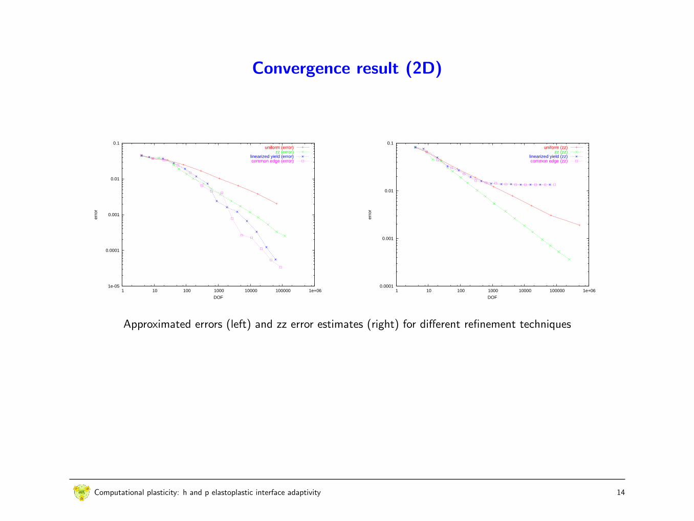
Convergence result (2D)
1e-05
0.0001
0.001
0.01
0.1
1 10 100 1000 10000 100000 1e+06
erro
r
DOF
uniform (error)zz (error)
linearized yield (error)common edge (error)
0.0001
0.001
0.01
0.1
1 10 100 1000 10000 100000 1e+06
erro
r
DOF
uniform (zz)zz (zz)
linearized yield (zz)common edge (zz)
Approximated errors (left) and zz error estimates (right) for different refinement techniques
Computational plasticity: h and p elastoplastic interface adaptivity 14

text
1e-05
0.0001
0.001
0.01
0.1
1 10 100 1000 10000 100000
erro
r
DOF
linearized yield (error)common edge (error)
linearized yield (zz)common edge (zz)
Failure of ZZ estimation in elastoplasticity???
Computational plasticity: h and p elastoplastic interface adaptivity 15
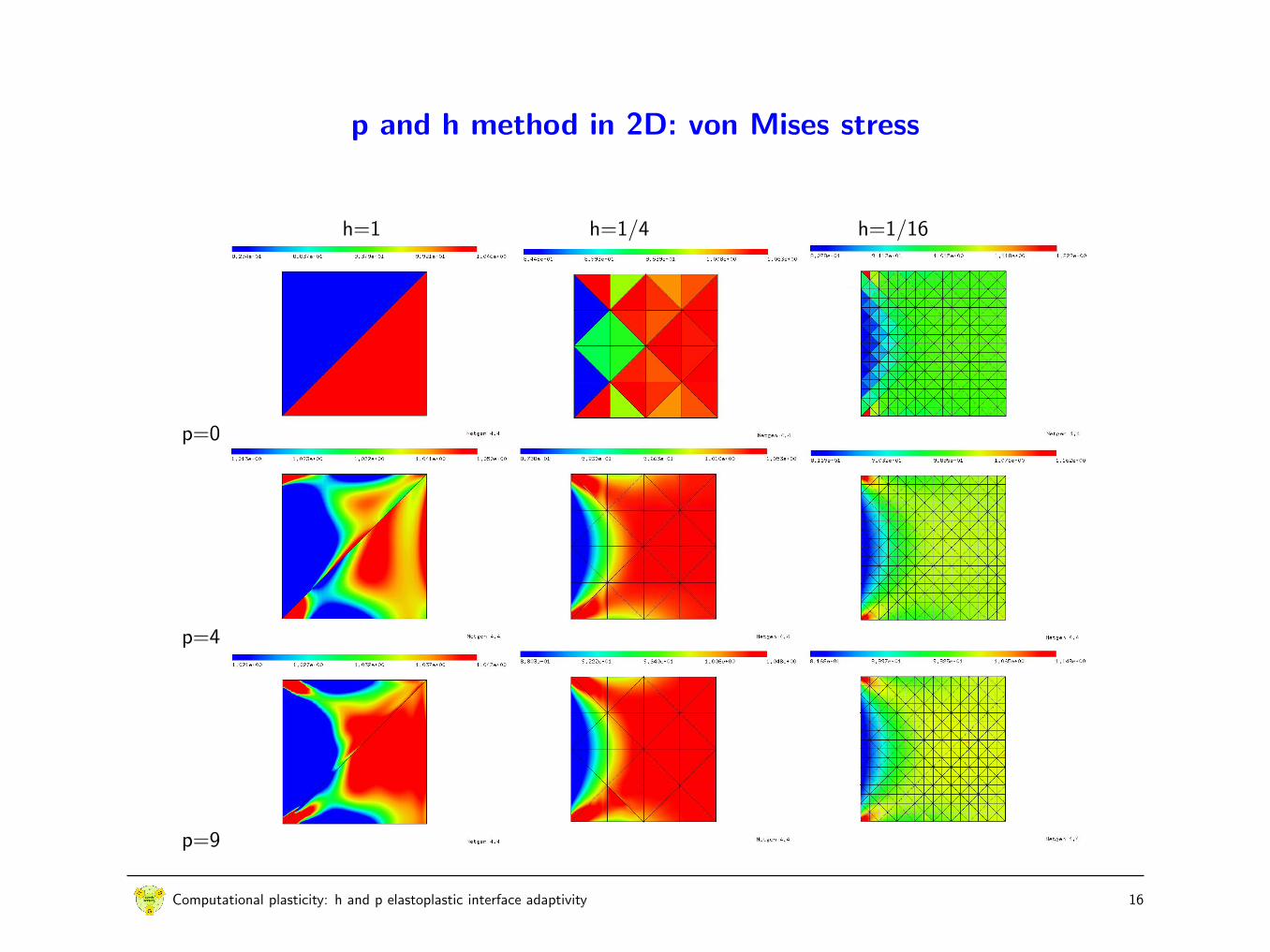
p and h method in 2D: von Mises stress
h=1 h=1/4 h=1/16
p=0
p=4
p=9
Computational plasticity: h and p elastoplastic interface adaptivity 16

p and h method in 3D: von Mises stress
For visualization reasons the stresses are projected onto a H1 function
h=1 h=1/2 h=1/4
p=0
p=1
p=3
Computational plasticity: h and p elastoplastic interface adaptivity 17

Conclusions
We have considered:
• Problem formulation and discretization
• Minimization: 3D time-dependent algorithm
• Numerical experiments
– Interface adaptivity
– p - version
Computational plasticity: h and p elastoplastic interface adaptivity 18

Conclusions
We have considered:
• Problem formulation and discretization
• Minimization: 3D time-dependent algorithm
• Numerical experiments
– Interface adaptivity
– p - version
Outlook
• Combined hpr methods
– h, r: Singularities
– p: Smooth solutions
• Level sets use for elastoplastic interface identification
• Application to shells
Computational plasticity: h and p elastoplastic interface adaptivity 18