Computational optimization of gas compressor stations ...

Math Meth Oper Res (2016) 83:409–444DOI 10.1007/s00186-016-0533-5

ORIGINAL ARTICLE

Computational optimization of gas compressor stations:MINLP models versus continuous reformulations

Daniel Rose1 · Martin Schmidt2,3 ·Marc C. Steinbach1 · Bernhard M. Willert4

Received: 3 March 2015 / Accepted: 19 January 2016 / Published online: 25 February 2016© The Author(s) 2016. This article is published with open access at Springerlink.com

Abstract When considering cost-optimal operation of gas transport networks, com-pressor stations play themost important role. Propermodeling of these stations leads tononconvex mixed-integer nonlinear optimization problems. In this article, we give anisothermal and stationary description of compressor stations, state MINLP and GDPmodels for operating a single station, and discuss several continuous reformulationsof the problem. The applicability and relevance of different model formulations, espe-cially of those without discrete variables, is demonstrated by a computational study onboth academic examples and real-world instances. In addition, we provide preliminarycomputational results for an entire network.

Keywords Discrete-continuous nonlinear optimization · Gas networks · Gascompressor stations · Mixed-integer optimization · Continuous reformulations

Mathematics Subject Classification 90-08 · 90C11 · 90C30 · 90C33 · 90C90

B Martin [email protected]

Daniel [email protected]

Marc C. [email protected]

1 Institute for Applied Mathematics, Leibniz Universität Hannover, Welfengarten 1, 30167Hannover, Germany

2 Discrete Optimization, Friedrich-Alexander-Universität Erlangen-Nürnberg, Cauerstr. 11, 91058Erlangen, Germany

3 Energie Campus Nürnberg, Fürther Str. 250, 90429 Nürnberg, Germany

4 Zur alten Zimmerei 6, 30952 Ronnenberg, Germany

123

http://crossmark.crossref.org/dialog/?doi=10.1007/s00186-016-0533-5&domain=pdf

410 D. Rose et al.

1 Introduction

Natural gas is one of the most important energy sources. In 2013, it accounted for 25%of the fossil energy used in Europe (Eurostat 2013). It is used in industrial processes,for heating, and, more recently, for natural gas vehicles. Especially in Germany, its lowprice leads to its role as a “bridging energy” during the transition to a future energymixbased primarily on regenerative energy. In Europe, natural gas is transported throughpipeline networkswith a total length of 100,000km.Gas transport in pipeline networksis pressure-driven, i.e., the gas flows from higher to lower pressure. Thus, pipeline-based gas transport requires compressor stations. The power required to compress thegas is delivered by drives that use either electrical power or gas from the networkitself. The energy consumption of compressors is responsible for a large fraction ofthe variable operating costs of a gas network.

In this article we focus on the stationary optimization of a single compressor station.More specifically, we consider fixed boundary conditions, i.e., fixed inflow and outflowpressures together with a fixed throughput, and ask the following questions:

– Can the station be operated in a way that satisfies the given boundary conditions?In other words: are those boundary conditions feasible?

– If the boundary conditions are feasible: What is a minimum cost operation thatsatisfies the boundary condition?

Transport of natural gas has been a rich source of mathematical optimization prob-lems for roughly half a century. The first publications on optimization in gas networksaddress tree-like or gun-barrel topologies with dynamic programming as a solutiontechnique (Wong and Larson 1968a, b); see Carter (1998) for a later survey. In thefollowing, we give a brief overview on mathematical optimization in this field. Moreextensive reviews can be found in Koch et al. (2015).

One main branch of research investigates the problems of minimum cost operationand feasibility testing for the stationary as well as the transient case. These problemsrequire models of complete gas networks comprising various types of elements likepipes, compressors, (control) valves, etc. The combination of nonlinear gas physicswith the switching of controllable network elements typically leads to mixed-integernonlinear optimization models (MINLPs); see, e.g., Cobos-Zaleta et al. (2002) andDomschke et al. (2011). One standard approach for tackling these MINLPs is theapplication of (piecewise) linearizations of the nonlinearities in order to reduce theproblems to mixed-integer linear models (MILPs) (Geißler 2011; Geißler et al. 2013;Martin et al. 2006, 2007; Martin and Möller 2005). Other investigations focus on thenonlinear aspects under fixed discrete controls (Ehrhardt and Steinbach 2004, 2005;Schmidt et al. 2015a, c; Steinbach 2007), or attempt to approximate discrete aspectsby continuous reformulations (Schmidt 2013; Schmidt et al. 2013, 2015b). For morereferences and reviews in the areas of cost minimization and feasibility testing werefer to Koch et al. (2015) and, especially, the chapter Schewe et al. (2015) therein.

The second major research branch that we want to highlight considers selectedtypes of network elements and studies them in more detail. For pipes, theoreticalstudies include the controllability and stabilization of the governing system of partialdifferential equations, the Euler equations (cf. Banda and Herty 2008; Banda et al.

123

Computational optimization of gas compressor stations… 411

2006; Brouwer et al. 2011; Gugat et al. 2015). The best-investigated problem forcompressor stations is the one considered in this paper, which is of nonconvexMINLPtype: minimum cost operation under given boundary conditions (Carter 1996; Carteret al. 1994; Jenícek and Králik 1993; Osiadacz 1980; Wright et al. 1998). See alsoKrálik (1993) for a simulation based model of compressor stations and Odom andMuster (2009) for a recent survey onmodeling centrifugal gas compressors. As alreadymentioned, the compressor stations are the dominant variable cost factor in gas networkoperation.

In this article we study discrete-continuous models for the problem of minimumcost compressor station operation. We give an almost complete isothermal descriptionof all relevant devices and their interplay. This description is comparable in accu-racy with isothermal simulation models. However, we neglect some minor modelaspects that would only complicate the presentation without influencing the solutionssignificantly. We explicitly mention these simplifications later in the description ofthe considered problem. The specific structure of the resulting MINLP allows for alarge variety of continuous reformulations that will be discussed in detail and that areapplied to the problem under consideration. The approach of continuous reformulationis in line with recent publications that develop techniques based on mathematical pro-grams with equilibrium constraints (MPECs) for reformulating other discrete aspectsof network optimization models (Pfetsch et al. 2015; Schmidt 2013; Schmidt et al.2013, 2015b). Thus, by combining the MPEC techniques from the cited publicationswith the reformulation schemes discussed in this paper, it is possible to state purelycontinuous NLP type models of the genuinely discrete-continuous problems of mini-mum cost operation or feasibility testing. The outcome of this achievement is twofold.First, it allows us to state highly detailed models of gas networks. This in particu-lar is not viable with approaches based on linearizations since the resulting MILPmodels tend to be very hard for state-of-the-art MILP solvers. Second, it allows usto solve the resulting models with local NLP solvers, which are typically faster thanglobal MI(N)LP solvers. Obviously, this comes at the price of finding only locallyoptimal solutions. For further applications of continuous reformulations of discrete-continuous optimization problems, especially in the field of process engineering, seeBaumrucker et al. (2008), Kraemer et al. (2007), Kraemer and Marquardt (2010), andStein et al. (2004). We remark that, despite the fact that continuous reformulations arebeing used in practice, an extensive numerical study like ours is yet missing in theliterature.

The paper is organized as follows. The problem of optimizing a gas compressor sta-tion under steady-state boundary conditions is presented in Sect. 2. Afterwards, Sect. 3introduces a mixed-integer nonlinear formulation of the problem and briefly discussesan equivalent general disjunctive programming formulation. Then, in Sect. 4, the con-cept of pseudo NCP (nonlinear complementarity problem) functions is introduced anda collection of continuous reformulation techniques is discussed that can be appliedto the MINLP model of Sect. 3. These reformulations are applied to artificial andreal-world compressor stations in Sect. 5 and the solutions are compared. In addition,this section also provides preliminary results for an entire large-scale network that isfully reformulated using continuous variables and smooth constraints. Finally, Sect. 6gives some remarks on further work and open questions.

123

412 D. Rose et al.

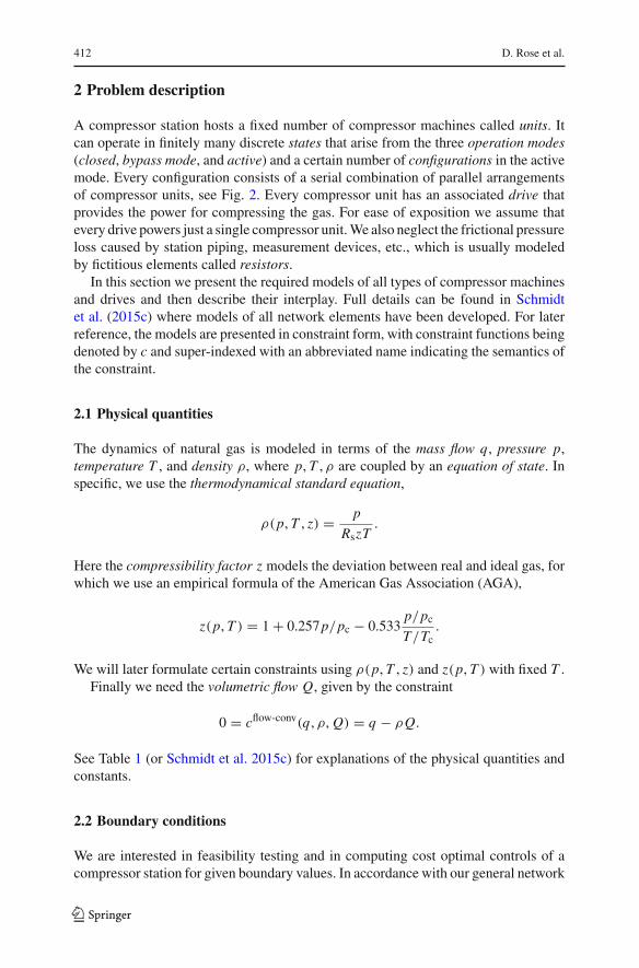
2 Problem description

A compressor station hosts a fixed number of compressor machines called units. Itcan operate in finitely many discrete states that arise from the three operation modes(closed, bypass mode, and active) and a certain number of configurations in the activemode. Every configuration consists of a serial combination of parallel arrangementsof compressor units, see Fig. 2. Every compressor unit has an associated drive thatprovides the power for compressing the gas. For ease of exposition we assume thatevery drive powers just a single compressor unit.We also neglect the frictional pressureloss caused by station piping, measurement devices, etc., which is usually modeledby fictitious elements called resistors.

In this section we present the required models of all types of compressor machinesand drives and then describe their interplay. Full details can be found in Schmidtet al. (2015c) where models of all network elements have been developed. For laterreference, the models are presented in constraint form, with constraint functions beingdenoted by c and super-indexed with an abbreviated name indicating the semantics ofthe constraint.

2.1 Physical quantities

The dynamics of natural gas is modeled in terms of the mass flow q, pressure p,temperature T , and density ρ, where p, T , ρ are coupled by an equation of state. Inspecific, we use the thermodynamical standard equation,

ρ(p, T , z) = p

RszT.

Here the compressibility factor z models the deviation between real and ideal gas, forwhich we use an empirical formula of the American Gas Association (AGA),

z(p, T ) = 1 + 0.257p/pc − 0.533p/pcT/Tc

.

We will later formulate certain constraints using ρ(p, T , z) and z(p, T ) with fixed T .Finally we need the volumetric flow Q, given by the constraint

0 = cflow-conv(q, ρ, Q) = q − ρQ.

See Table 1 (or Schmidt et al. 2015c) for explanations of the physical quantities andconstants.

2.2 Boundary conditions

We are interested in feasibility testing and in computing cost optimal controls of acompressor station for given boundary values. In accordance with our general network

123


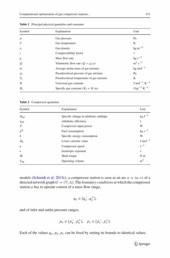
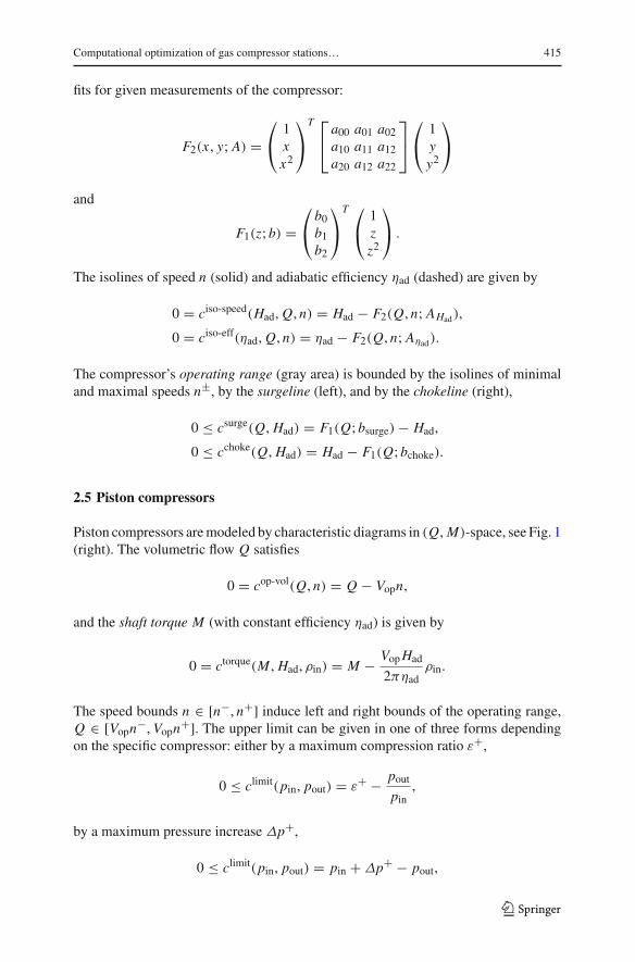
Table 1 Principal physical quantities and constants

Symbol Explanation Unit

p Gas pressure Pa

T Gas temperature K

ρ Gas density kg m−3

z Compressibility factor 1

q Mass flow rate kg s−1

Q Volumetric flow rate (Q = q/ρ) m3 s−1

m Average molar mass of gas mixture kg mol−1

pc Pseudocritical pressure of gas mixture Pa

Tc Pseudocritical temperature of gas mixture K

R Universal gas constant J mol−1 K−1

Rs Specific gas constant (Rs = R/m) J kg−1 K−1

Table 2 Compressor quantities

Symbol Explanation Unit

Had Specific change in adiabatic enthalpy kg J−1

ηad Adiabatic efficiency 1

P Compressor input power W

qfc Fuel consumption kg s−1

b Specific energy consumption W

Hu Lower calorific value J mol−1

n Compressor speed s−1

κ Isentropic exponent 1

M Shaft torque N m

Vop Operating volume m3

models (Schmidt et al. 2015c), a compressor station is seen as an arc a = (u, v) of adirected network graphG = (V,A). The boundary conditions atwhich the compressorstation a has to operate consist of a mass flow range,

qa ∈ [q−a , q

+a ],

and of inlet and outlet pressure ranges,

pu ∈ [p−u , p

+u ], pv ∈ [p−

v , p+v ].

Each of the values qa , pu , pv can be fixed by setting its bounds to identical values.

123

414 D. Rose et al.

0 5 100

10

20

30

0 1 2 30

1

2

3

·107

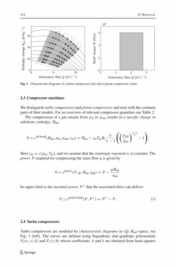
Fig. 1 Characteristic diagrams of a turbo compressor (left) and a piston compressor (right)

2.3 Compressor machines

We distinguish turbo compressors and piston compressors and start with the commonparts of their models. For an overview of relevant compressor quantities see Table 2.

The compression of a gas stream from pin to pout results in a specific change inadiabatic enthalpy, Had:

0 = cad-head(Had, pin, pout, zin) = Had − zinTinRsκ

κ − 1

((poutpin

) κ−1κ − 1

).

Here zin = z(pin, Tin), and we assume that the isentropic exponent κ is constant. Thepower P required for compressing the mass flow q is given by

0 = cpower(P , q, Had, ηad) = P − qHad

ηad.

Its upper limit is the maximal power P+ that the associated drive can deliver:

0 ≤ cpower-limit(P , P+) = P+ − P . (1)

2.4 Turbo compressors

Turbo compressors are modeled by characteristic diagrams in (Q, Had)-space, seeFig. 1 (left). The curves are defined using biquadratic and quadratic polynomialsF2(x , y; A) and F1(z; b) whose coefficients A and b are obtained from least-squares

123


fits for given measurements of the compressor:

F2(x , y; A) =⎛⎝ 1

xx2

⎞⎠

T ⎡⎣a00 a01 a02a10 a11 a12a20 a12 a22

⎤⎦

⎛⎝ 1

yy2

⎞⎠

and

F1(z; b) =⎛⎝ b0b1b2

⎞⎠

T ⎛⎝ 1

zz2

⎞⎠ .

The isolines of speed n (solid) and adiabatic efficiency ηad (dashed) are given by

0 = ciso-speed(Had, Q, n) = Had − F2(Q, n; AHad),

0 = ciso-eff(ηad, Q, n) = ηad − F2(Q, n; Aηad).

The compressor’s operating range (gray area) is bounded by the isolines of minimaland maximal speeds n±, by the surgeline (left), and by the chokeline (right),

0 ≤ csurge(Q, Had) = F1(Q; bsurge) − Had,

0 ≤ cchoke(Q, Had) = Had − F1(Q; bchoke).

2.5 Piston compressors

Piston compressors aremodeled by characteristic diagrams in (Q,M)-space, see Fig. 1(right). The volumetric flow Q satisfies

0 = cop-vol(Q, n) = Q − Vopn,

and the shaft torque M (with constant efficiency ηad) is given by

0 = ctorque(M , Had, ρin) = M − VopHad

2πηadρin.

The speed bounds n ∈ [n−, n+] induce left and right bounds of the operating range,Q ∈ [Vopn−, Vopn+]. The upper limit can be given in one of three forms dependingon the specific compressor: either by a maximum compression ratio ε+,

0 ≤ climit(pin, pout) = ε+ − poutpin

,

by a maximum pressure increase Δp+,

0 ≤ climit(pin, pout) = pin + Δp+ − pout,

123

416 D. Rose et al.

or by a maximum shaft torque M+,

0 ≤ climit(M) = M+ − M .

2.6 Drives

The four most frequently used drive types are gas turbines, gas driven motors, electricmotors, and steam turbines. Here we focus on the commonmodel aspects and considera generic “catchall” drive model that incorporates the two main aspects: the maximalpower P+ that the drive can deliver (cf. (1)),

0 = cmax-power(P+, n) = P+ − F2(n, Tamb; AP+), (2)

and its specific energy consumption b,

0 = cspec-ener-cons(b, P) = b − F1(P; ab). (3)

Here, Tamb denotes the ambient temperature at the compressor station and AP+ aswell as ab are the coefficients of the fitted (bi)quadratic polynomials. For specificdrive types, (2) or (3) may simplify or vanish completely. The fuel consumption of agas-powered drive is the mass flow qfc,

0 = cfuel-cons(qfc, b) = qfc − bm

Hu.

The fuel consumption of an electric drive is zero, 0 = cfuel-cons(qfc, b) = qfc.

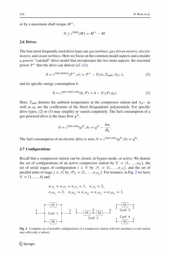
2.7 Configurations

Recall that a compressor station can be closed, in bypass mode, or active. We denotethe set of configurations of an active compressor station by C = {1, . . . , nC }, theset of serial stages of configuration i ∈ C by Si = {1, . . . , nSi }, and the set ofparallel units of stage j ∈ Si byPi j = {1, . . . , nPi j }. For instance, in Fig. 2 we haveC = {1, . . . , 4} and

nS1 = nS3 = nS4 = 1, nS2 = 2,

nP11 = 2, nP21 = nP22 = nP31 = nP41 = 1.

M1

M2

M1 M2

M1

M2

Fig. 2 Complete set of possible configurations of a compressor station with two machines (a real stationmay offer only a subset)

123


In what follows, we refer to individual compressor units by the index triple i jk.Given a triple (qa , pu , pv) of boundary values, the selected configuration i must

satisfy the following: the flow q j of every serial stage j ∈ Si equals qa and isdistributed over the nPi j parallel units:

qa = q j =∑

k∈Pi j

qi jk for all j ∈ Si .

Moreover, all parallel units in stage j ∈ Si have to increase the gas pressure to acommon outflow value pi , j+1, which becomes the inflow pressure of stage j + 1. Thefirst and last stages must satisfy pi1 = pu and pi ,nSi +1 = pv , respectively.

2.8 Objective function

There are various reasonable objective functions in our context, which can mainly becategorized as feasibility or optimization goals. If one merely wishes to know whethergiven boundary conditions are feasible, it suffices to use a zero objective, f ≡ 0.If the boundary conditions are infeasible, it may be useful to add slack variablesto a certain set of constraints and minimize the total infeasibility, measured by asuitable normof the vector of slack variables. The reader interested in problem-specificslack variable formulations for gas network planning is referred to Schmidt et al.(2015a).

If one is convinced of having feasible boundary conditions, it is straightforward tominimize operating costs, power, or fuel consumption. Specific objective functionswill be formulated after stating the optimization models in the following section.

3 Mixed-integer and general disjunctive programming models

One generic way tomodel the problem described in the previous section is presented inSect. 3.1: a mixed-integer nonlinear program (MINLP) that incorporates binary vari-ables for the discrete states of the compressor station.An equivalent general disjunctiveprogramming (GDP) formulation of the problem is given in Sect. 3.2. Continuousreformulations of the MINLP and GDP models are discussed later in Sect. 4.

One further possibility of tackling the problem is to enumerate all states of thecompressor station and solve all the resulting (continuous) problems by a local orglobal method. However, this is only suitable when single compressor stations areconsidered, whereas continuous reformulations can also be used for models of theentire transport network; cf. Sect. 5.5. Another way is to apply suitable heuristics, see,e.g., Schmidt et al. (2015b).

We denote individual continuous variables by x and discrete ones by s. Variablevectors are written with bold letters, like x or s. Sub-indices refer to correspondingelements of the compressor station or to sets of elements. In the constraint notation ofSect. 2,we nowalso use sub-indiceswith the samemeaning as for variables.Additionalsub-indices E or I distinguish equality and inequality constraints.

123

418 D. Rose et al.

3.1 MINLP formulation

With x ∈ Rn and s ∈ {0, 1}m , the optimization problem under consideration takes the

general MINLP form

minx,s

f (x, s) s.t. cE (x, s) = 0, cI (x, s) ≥ 0.

The boundary conditions correspond to the variable sub-vector xB = (qa , pu , pv).For a suitable formulation of the discrete decisions and their implications on other

parts of the model, we review the concept of indicator constraints.

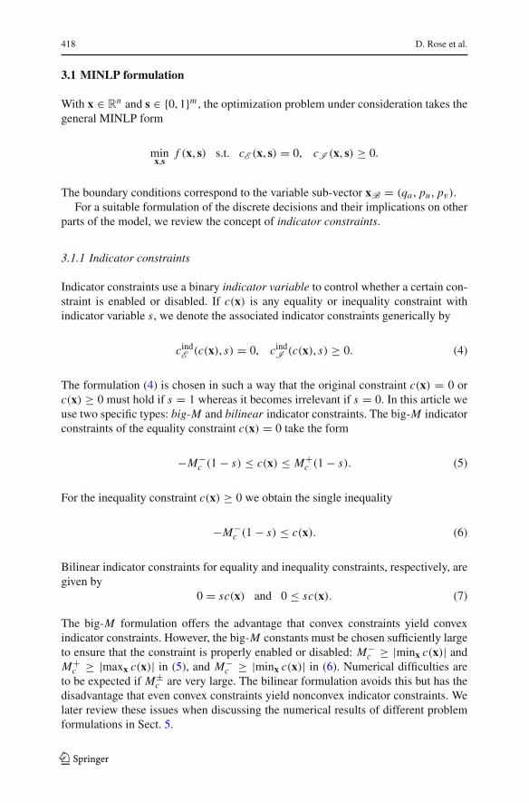
3.1.1 Indicator constraints

Indicator constraints use a binary indicator variable to control whether a certain con-straint is enabled or disabled. If c(x) is any equality or inequality constraint withindicator variable s, we denote the associated indicator constraints generically by

cindE (c(x), s) = 0, cindI (c(x), s) ≥ 0. (4)

The formulation (4) is chosen in such a way that the original constraint c(x) = 0 orc(x) ≥ 0 must hold if s = 1 whereas it becomes irrelevant if s = 0. In this article weuse two specific types: big-M and bilinear indicator constraints. The big-M indicatorconstraints of the equality constraint c(x) = 0 take the form

−M−c (1 − s) ≤ c(x) ≤ M+

c (1 − s). (5)

For the inequality constraint c(x) ≥ 0 we obtain the single inequality

−M−c (1 − s) ≤ c(x). (6)

Bilinear indicator constraints for equality and inequality constraints, respectively, aregiven by

0 = sc(x) and 0 ≤ sc(x). (7)

The big-M formulation offers the advantage that convex constraints yield convexindicator constraints. However, the big-M constants must be chosen sufficiently largeto ensure that the constraint is properly enabled or disabled: M−

c ≥ |minx c(x)| andM+

c ≥ |maxx c(x)| in (5), and M−c ≥ |minx c(x)| in (6). Numerical difficulties are

to be expected if M±c are very large. The bilinear formulation avoids this but has the

disadvantage that even convex constraints yield nonconvex indicator constraints. Welater review these issues when discussing the numerical results of different problemformulations in Sect. 5.

123


Finally we need two more notions: an indicator expression y is a term whose valueis y ≥ 1 if the associated state is enabled and zero otherwise, like s in (7). Conversely,a negation expression is a term whose value is y ≥ 1 if the associated state is disabledand zero otherwise, like 1 − s in (5), (6).

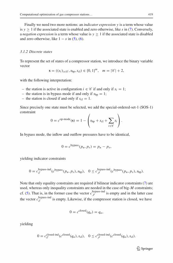
3.1.2 Discrete states

To represent the set of states of a compressor station, we introduce the binary variablevector

s = ((si )i∈C , sbp, scl) ∈ {0, 1}m , m = |C | + 2,

with the following interpretation:

– the station is active in configuration i ∈ C if and only if si = 1;– the station is in bypass mode if and only if sbp = 1;– the station is closed if and only if scl = 1.

Since precisely one state must be selected, we add the special-ordered-set-1 (SOS-1)constraint

0 = cop-mode(s) = 1 −⎛⎝sbp + scl +

∑i∈C

si

⎞⎠ .

In bypass mode, the inflow and outflow pressures have to be identical,

0 = cbypass(pu , pv) = pu − pv ,

yielding indicator constraints

0 = cbypass-indE (cbypass(pu , pv), sbp), 0 ≤ cbypass-indI (cbypass(pu , pv), sbp).

Note that only equality constraints are required if bilinear indicator constraints (7) areused, whereas only inequality constraints are needed in the case of big-M constraints;cf. (5). That is, in the former case the vector cbypass-indI is empty and in the latter case

the vector cbypass-indE is empty. Likewise, if the compressor station is closed, we have

0 = cclosed(qa) = qa ,

yielding

0 = cclosed-indE (cclosed(qa), scl), 0 ≤ cclosed-indI (cclosed(qa), scl).

123

420 D. Rose et al.

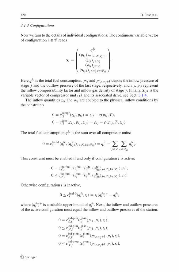
3.1.3 Configurations

Nowwe turn to the details of individual configurations. The continuous variable vectorof configuration i ∈ C reads

xi =

⎛⎜⎜⎜⎜⎝

qfci(pi j ) j=1,...,nSi +1

(zi j ) j∈Si

(ρi j ) j∈Si

(xi jk) j∈Si ,k∈Pi j

⎞⎟⎟⎟⎟⎠ .

Here qfci is the total fuel consumption, pi j and pi ,nSi +1 denote the inflow pressure ofstage j and the outflow pressure of the last stage, respectively, and zi j , ρi j representthe inflow compressibility factor and inflow gas density of stage j . Finally, xi jk is thevariable vector of compressor unit i jk and its associated drive, see Sect. 3.1.4.

The inflow quantities zi j and ρi j are coupled to the physical inflow conditions bythe constraints

0 = ccompri j (zi j , pi j ) = zi j − z(pi j , T ),

0 = cdensi j (ρi j , pi j , zi j ) = ρi j − ρ(pi j , T , zi j ).

The total fuel consumption qfci is the sum over all compressor units:

0 = cfuel-1i (qfci , (qfci jk) j∈Si ,k∈Pi j ) = qfci −

∑j∈Si

∑k∈Pi j

qfci jk .

This constraint must be enabled if and only if configuration i is active:

0 = cind-fuel-1E ,i (cfuel-1i (qfci , (qfci jk) j∈Si ,k∈Pi j ), si ),

0 ≤ cind-fuel-1I ,i (cfuel-1i (qfci , (qfci jk) j∈Si ,k∈Pi j ), si ).

Otherwise configuration i is inactive,

0 ≤ cfuel-0i (qfci , si ) = si (qfci )+ − qfci ,

where (qfci )+ is a suitable upper bound of qfci . Next, the inflow and outflow pressuresof the active configuration must equal the inflow and outflow pressures of the station:

0 = cind-p-inE ,i (cp-ini (pi1, pu), si ),

0 ≤ cind-p-inI ,i (cp-ini (pi1, pu), si ),

0 = cind-p-outE ,i (cp-outi (pi ,nSi +1, pv), si ),

0 ≤ cind-p-outI ,i (cp-outi (pi ,nSi +1, pv), si ),

123


where

0 = cp-ini (pi1, pu) = pi1 − pu ,

0 = cp-outi (pi ,nSi +1, pv) = pi ,nSi +1 − pv .

The flow distribution over the parallel units of every stage j finally completes theconfiguration model:

0 = cflowi j (qa , (qi jk)k∈Pi j ) = qa −∑

k∈Pi j

qi jk , j ∈ Si .

In summary, the equality constraints of configuration i read

0 = cE ,i (xB , xi , si ) =

⎛⎜⎜⎜⎜⎜⎜⎜⎜⎝

(ccompri j (zi j , pi j )) j∈Si

(cdensi j (ρi j , pi j , zi j )) j∈Si

cind-fuel-1E ,i (qfci , (qfci jk) j∈Si ,k∈Pi j , si )

cind-p-inE ,i (pi1, pu , si )

cind-p-outE ,i (pi ,nSi +1, pv , si )(cflowi j (qa , (qi jk)k∈Pi j )) j∈Si

⎞⎟⎟⎟⎟⎟⎟⎟⎟⎠

and the inequality constraints are given by

0 ≤ cI ,i (xB , xi , si ) =

⎛⎜⎜⎜⎝cind-fuel-1I ,i (qfci , (q

fci jk) j∈Si ,k∈Pi j , si )

cind-fuel-0I ,i (qfci , si )

cind-p-inI ,i (pi1, pu , si )

cind-p-outI ,i (pi ,nSi +1, pv , si )

⎞⎟⎟⎟⎠ .

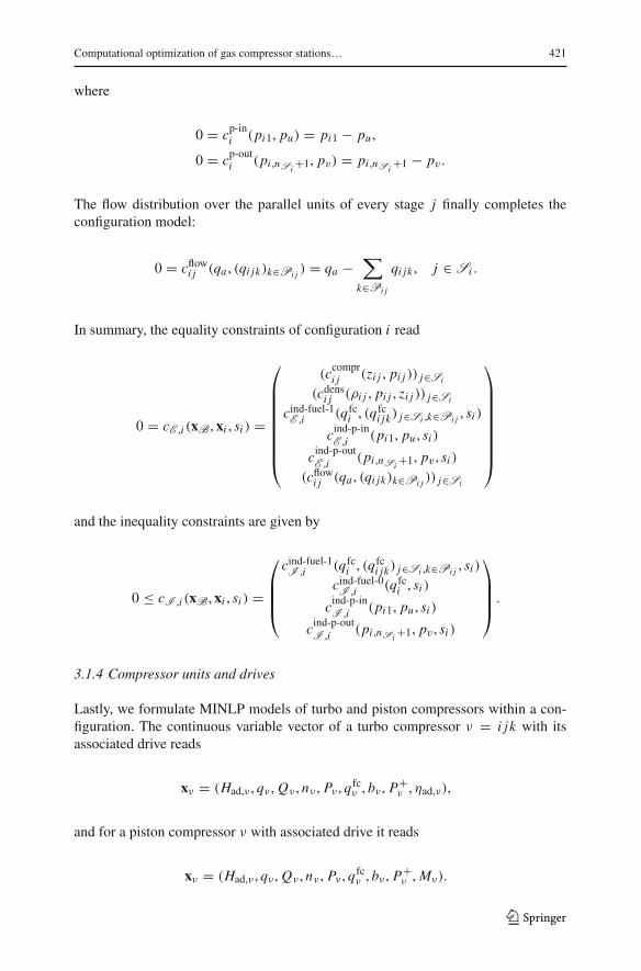
3.1.4 Compressor units and drives

Lastly, we formulate MINLP models of turbo and piston compressors within a con-figuration. The continuous variable vector of a turbo compressor ν = i jk with itsassociated drive reads

xν = (Had,ν , qν , Qν , nν , Pν , qfcν , bν , P

+ν , ηad,ν),

and for a piston compressor ν with associated drive it reads

xν = (Had,ν , qν , Qν , nν , Pν , qfcν , bν , P

+ν ,Mν).

123

422 D. Rose et al.

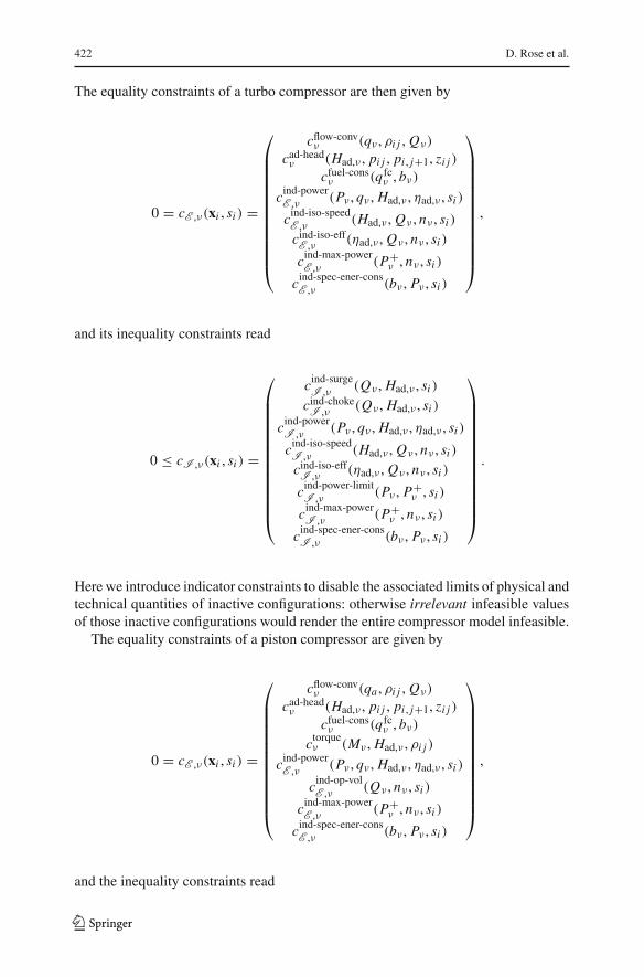
The equality constraints of a turbo compressor are then given by

0 = cE ,ν(xi , si ) =

⎛⎜⎜⎜⎜⎜⎜⎜⎜⎜⎜⎜⎜⎝

cflow-convν (qν , ρi j , Qν)

cad-headν (Had,ν , pi j , pi , j+1, zi j )cfuel-consν (qfcν , bν)

cind-powerE ,ν (Pν , qν , Had,ν , ηad,ν , si )

cind-iso-speedE ,ν (Had,ν , Qν , nν , si )cind-iso-effE ,ν (ηad,ν , Qν , nν , si )

cind-max-powerE ,ν (P+

ν , nν , si )

cind-spec-ener-consE ,ν (bν , Pν , si )

⎞⎟⎟⎟⎟⎟⎟⎟⎟⎟⎟⎟⎟⎠,

and its inequality constraints read

0 ≤ cI ,ν(xi , si ) =

⎛⎜⎜⎜⎜⎜⎜⎜⎜⎜⎜⎜⎜⎜⎝

cind-surgeI ,ν (Qν , Had,ν , si )cind-chokeI ,ν (Qν , Had,ν , si )

cind-powerI ,ν (Pν , qν , Had,ν , ηad,ν , si )

cind-iso-speedI ,ν (Had,ν , Qν , nν , si )cind-iso-effI ,ν (ηad,ν , Qν , nν , si )

cind-power-limitI ,ν (Pν , P+

ν , si )

cind-max-powerI ,ν (P+

ν , nν , si )

cind-spec-ener-consI ,ν (bν , Pν , si )

⎞⎟⎟⎟⎟⎟⎟⎟⎟⎟⎟⎟⎟⎟⎠.

Here we introduce indicator constraints to disable the associated limits of physical andtechnical quantities of inactive configurations: otherwise irrelevant infeasible valuesof those inactive configurations would render the entire compressor model infeasible.

The equality constraints of a piston compressor are given by

0 = cE ,ν(xi , si ) =

⎛⎜⎜⎜⎜⎜⎜⎜⎜⎜⎜⎜⎜⎝

cflow-convν (qa , ρi j , Qν)

cad-headν (Had,ν , pi j , pi , j+1, zi j )cfuel-consν (qfcν , bν)

ctorqueν (Mν , Had,ν , ρi j )

cind-powerE ,ν (Pν , qν , Had,ν , ηad,ν , si )

cind-op-volE ,ν (Qν , nν , si )

cind-max-powerE ,ν (P+

ν , nν , si )

cind-spec-ener-consE ,ν (bν , Pν , si )

⎞⎟⎟⎟⎟⎟⎟⎟⎟⎟⎟⎟⎟⎠,

and the inequality constraints read

123


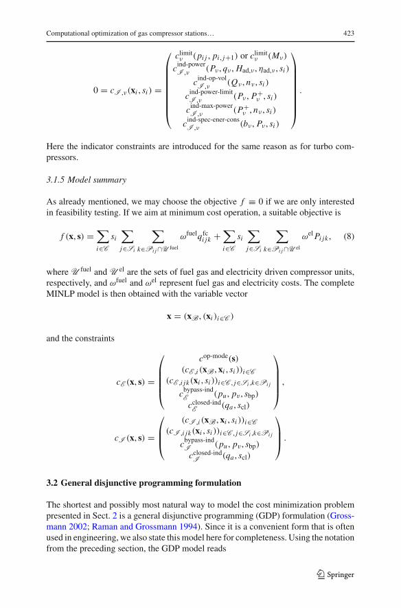
0 = cI ,ν(xi , si ) =

⎛⎜⎜⎜⎜⎜⎜⎜⎜⎝

climitν (pi j , pi , j+1) or climit

ν (Mν)

cind-powerI ,ν (Pν , qν , Had,ν , ηad,ν , si )

cind-op-volI ,ν (Qν , nν , si )

cind-power-limitI ,ν (Pν , P+

ν , si )

cind-max-powerI ,ν (P+

ν , nν , si )

cind-spec-ener-consI ,ν (bν , Pν , si )

⎞⎟⎟⎟⎟⎟⎟⎟⎟⎠.

Here the indicator constraints are introduced for the same reason as for turbo com-pressors.

3.1.5 Model summary

As already mentioned, we may choose the objective f ≡ 0 if we are only interestedin feasibility testing. If we aim at minimum cost operation, a suitable objective is

f (x, s) =∑i∈C

si∑j∈Si

∑k∈Pi j∩U fuel

ωfuelqfci jk +∑i∈C

si∑j∈Si

∑k∈Pi j∩U el

ωelPi jk , (8)

where U fuel and U el are the sets of fuel gas and electricity driven compressor units,respectively, and ωfuel and ωel represent fuel gas and electricity costs. The completeMINLP model is then obtained with the variable vector

x = (xB , (xi )i∈C )

and the constraints

cE (x, s) =

⎛⎜⎜⎜⎜⎝

cop-mode(s)(cE ,i (xB , xi , si ))i∈C

(cE ,i jk(xi , si ))i∈C , j∈Si ,k∈Pi j

cbypass-indE (pu , pv , sbp)cclosed-indE (qa , scl)

⎞⎟⎟⎟⎟⎠ ,

cI (x, s) =

⎛⎜⎜⎝

(cI ,i (xB , xi , si ))i∈C(cI ,i jk(xi , si ))i∈C , j∈Si ,k∈Pi j

cbypass-indI (pu , pv , sbp)cclosed-indI (qa , scl)

⎞⎟⎟⎠ .

3.2 General disjunctive programming formulation

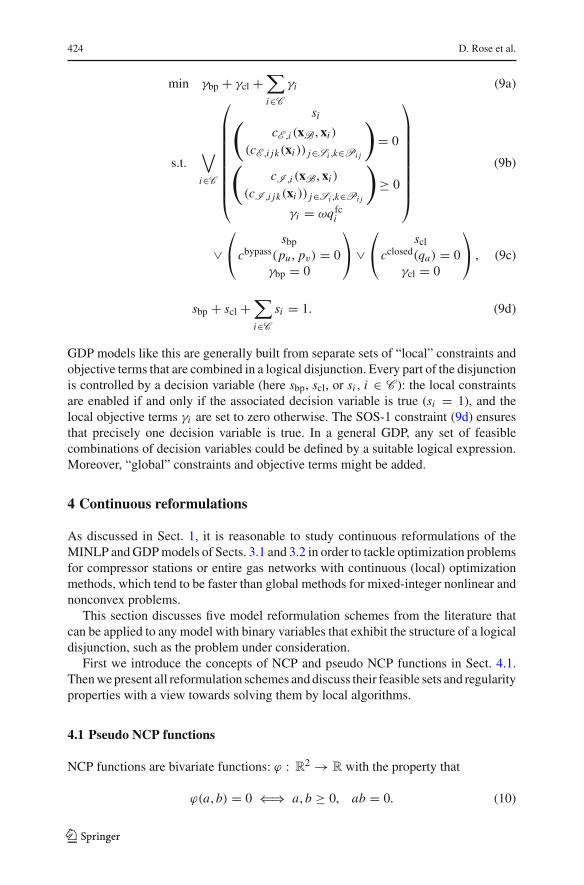
The shortest and possibly most natural way to model the cost minimization problempresented in Sect. 2 is a general disjunctive programming (GDP) formulation (Gross-mann 2002; Raman and Grossmann 1994). Since it is a convenient form that is oftenused in engineering, we also state this model here for completeness. Using the notationfrom the preceding section, the GDP model reads

123

424 D. Rose et al.

min γbp + γcl +∑i∈C

γi (9a)

s.t.∨i∈C

⎛⎜⎜⎜⎜⎜⎜⎜⎜⎜⎝

si(cE ,i (xB , xi )

(cE ,i jk(xi )) j∈Si ,k∈Pi j

)= 0

(cI ,i (xB , xi )

(cI ,i jk(xi )) j∈Si ,k∈Pi j

)≥ 0

γi = ωqfci

⎞⎟⎟⎟⎟⎟⎟⎟⎟⎟⎠

(9b)

∨⎛⎝ sbpcbypass(pu , pv) = 0

γbp = 0

⎞⎠ ∨

⎛⎝ sclcclosed(qa) = 0

γcl = 0

⎞⎠ , (9c)

sbp + scl +∑i∈C

si = 1. (9d)

GDP models like this are generally built from separate sets of “local” constraints andobjective terms that are combined in a logical disjunction. Every part of the disjunctionis controlled by a decision variable (here sbp, scl, or si , i ∈ C ): the local constraintsare enabled if and only if the associated decision variable is true (si = 1), and thelocal objective terms γi are set to zero otherwise. The SOS-1 constraint (9d) ensuresthat precisely one decision variable is true. In a general GDP, any set of feasiblecombinations of decision variables could be defined by a suitable logical expression.Moreover, “global” constraints and objective terms might be added.

4 Continuous reformulations

As discussed in Sect. 1, it is reasonable to study continuous reformulations of theMINLP andGDPmodels of Sects. 3.1 and 3.2 in order to tackle optimization problemsfor compressor stations or entire gas networks with continuous (local) optimizationmethods, which tend to be faster than global methods for mixed-integer nonlinear andnonconvex problems.

This section discusses five model reformulation schemes from the literature thatcan be applied to any model with binary variables that exhibit the structure of a logicaldisjunction, such as the problem under consideration.

First we introduce the concepts of NCP and pseudo NCP functions in Sect. 4.1.Thenwepresent all reformulation schemes anddiscuss their feasible sets and regularityproperties with a view towards solving them by local algorithms.

4.1 Pseudo NCP functions

NCP functions are bivariate functions: ϕ : R2 → R with the property that

ϕ(a, b) = 0 ⇐⇒ a, b ≥ 0, ab = 0. (10)

123


Classical NCP functions include, e.g., the minimum function ϕmin(a, b) = min(a, b)and the Fischer–Burmeister function (Fischer 1992),

ϕFB(a, b) =√a2 + b2 − (a + b).

See Sun and Qi (1999) and the references therein for an overview of NCP functions.NCP functions can be used to replace binary variables with continuous variables.However, the right-hand side of (10) introduces some difficulties if it is consideredfrom an NLP perspective. The constraints a, b ≥ 0, ab = 0 lead to mathematicalprograms with equilibrium constraints (MPECs). The problem is that standard NLPregularity concepts like the linear independence constraint qualification (LICQ) orthe Mangasarian–Fromovitz constraint qualification (MFCQ) are violated at everyfeasible point of an MPEC (Ye and Zhu 1995); see Luo et al. (1996) for an overviewof the theory and applications of MPECs. However, the nonnegativity constraints in(10) are not needed for the reformulations discussed below. This leads us to extendthe class of NCP functions: We call a function φ : R2 → R a pseudo NCP function if

φ(a, b) = 0 �⇒ a = 0 or b = 0.

In the remainder of this article we use the following two pseudo NCP functions:

φprod(a, b) := ab, φFB(a, b) := ϕFB(a, b).

Note that the Fischer–Burmeister φFB function has a lack of regularity, whereas theproduct formulation φprod is favorable since we do not have to impose nonnegativityconstraints here as in the classical NCP setting.

4.2 Reformulation schemes

It iswell-known that local solvers tend to be very sensitive to the specific formulation ofa nonlinear model. This is the reason why it is often useful in practice to have differentequivalent formulations to evaluatewhich formulation is best suited for the used solver.In this section we discuss five schemes that allow to reformulate the MINLP andGDP models of Sects. 3.1 and 3.2 with continuous variables and additional smoothconstraints. Since the geometry of the feasible regions of the resulting continuousmodels and their regularity properties also have a strong influence on the solutionprocess, we analyze these aspects for every reformulation.

To be applicable in the context of the model of Sect. 3.1, the reformulations haveto possess the following properties:

1. Every feasible solution of the reformulation has to be uniquely translatable into afeasible solution of the original MINLP (or GDP). This means that there exists amapping (a left-total right-unique relation) from the feasible set of the reformula-tion to the feasible set of the original model.

2. For every binary variable s ∈ {0, 1}, the reformulation has variables from whichindicator and negation expressions can be constructed (cf. Sect. 3.1.1).

123

426 D. Rose et al.

3. The reformulation has variables from which the SOS-1 constraint can be con-structed.

In what follows, we only present the representations of a set of binary variabless1, . . . , sm ∈ {0, 1} together with the SOS-1 constraint∑m

i=1 si = 1, rather than statingcomplete reformulated models. The latter can easily be reproduced from Sect. 3.1. Wefrequently use the setsM := {1, . . . ,m} and Mi := M \ {i}.

As already stated in Sect. 1, all reformulation schemes below can be found in theexisting literature—in particular, see Baumrucker et al. (2008), Kraemer and Mar-quardt (2010), and Stein et al. (2004)—except that we use pseudo NCP functionsrather than NCP functions.

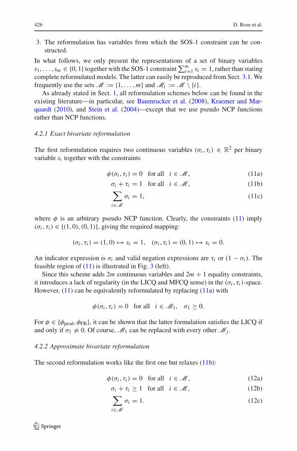
4.2.1 Exact bivariate reformulation

The first reformulation requires two continuous variables (σi , τi ) ∈ R2 per binary

variable si together with the constraints

φ(σi , τi ) = 0 for all i ∈ M , (11a)

σi + τi = 1 for all i ∈ M , (11b)∑i∈M

σi = 1, (11c)

where φ is an arbitrary pseudo NCP function. Clearly, the constraints (11) imply(σi , τi ) ∈ {(1, 0), (0, 1)}, giving the required mapping:

(σi , τi ) = (1, 0) �→ si = 1, (σi , τi ) = (0, 1) �→ si = 0.

An indicator expression is σi and valid negation expressions are τi or (1 − σi ). Thefeasible region of (11) is illustrated in Fig. 3 (left).

Since this scheme adds 2m continuous variables and 2m + 1 equality constraints,it introduces a lack of regularity (in the LICQ and MFCQ sense) in the (σi , τi )-space.However, (11) can be equivalently reformulated by replacing (11a) with

φ(σi , τi ) = 0 for all i ∈ M1, σ1 ≥ 0.

For φ ∈ {φprod,φFB}, it can be shown that the latter formulation satisfies the LICQ ifand only if σ1 = 0. Of course, M1 can be replaced with every other M j .

4.2.2 Approximate bivariate reformulation

The second reformulation works like the first one but relaxes (11b):

φ(σi , τi ) = 0 for all i ∈ M , (12a)

σi + τi ≥ 1 for all i ∈ M , (12b)∑i∈M

σi = 1. (12c)

123


Fig. 3 Left: Feasible set of the exact bivariate reformulation. The axes are the feasible sets of (11a). Togetherwith (11b) the feasible set {(1, 0), (0, 1)} (bullets) remains. Right: Feasible set of the approximate bivariatereformulation. The axes are the feasible sets of (12a) and the shaded area is the feasible region of (12b).The intersection consists of the two disjoint bold lines

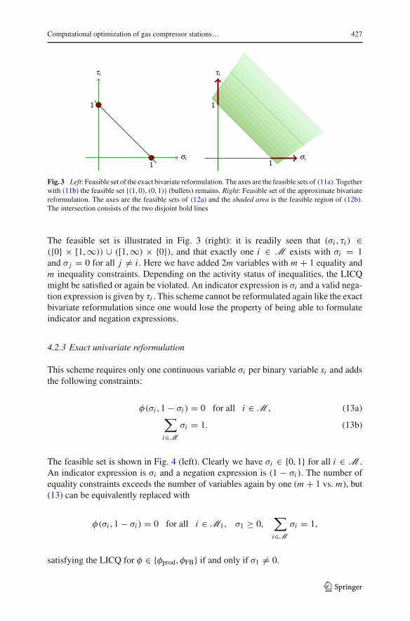
The feasible set is illustrated in Fig. 3 (right): it is readily seen that (σi , τi ) ∈({0} × [1,∞)) ∪ ([1,∞) × {0}), and that exactly one i ∈ M exists with σi = 1and σ j = 0 for all j = i . Here we have added 2m variables with m + 1 equality andm inequality constraints. Depending on the activity status of inequalities, the LICQmight be satisfied or again be violated. An indicator expression is σi and a valid nega-tion expression is given by τi . This scheme cannot be reformulated again like the exactbivariate reformulation since one would lose the property of being able to formulateindicator and negation expressions.

4.2.3 Exact univariate reformulation

This scheme requires only one continuous variable σi per binary variable si and addsthe following constraints:

φ(σi , 1 − σi ) = 0 for all i ∈ M , (13a)∑i∈M

σi = 1. (13b)

The feasible set is shown in Fig. 4 (left). Clearly we have σi ∈ {0, 1} for all i ∈ M .An indicator expression is σi and a negation expression is (1 − σi ). The number ofequality constraints exceeds the number of variables again by one (m + 1 vs. m), but(13) can be equivalently replaced with

φ(σi , 1 − σi ) = 0 for all i ∈ M1, σ1 ≥ 0,∑i∈M

σi = 1,

satisfying the LICQ for φ ∈ {φprod,φFB} if and only if σ1 = 0.

123

428 D. Rose et al.

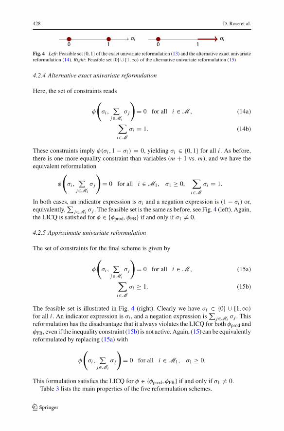
Fig. 4 Left: Feasible set {0, 1} of the exact univariate reformulation (13) and the alternative exact univariatereformulation (14). Right: Feasible set {0} ∪ [1,∞) of the alternative univariate reformulation (15)

4.2.4 Alternative exact univariate reformulation

Here, the set of constraints reads

φ

(σi ,

∑j∈Mi

σ j

)= 0 for all i ∈ M , (14a)

∑i∈M

σi = 1. (14b)

These constraints imply φ(σi , 1 − σi ) = 0, yielding σi ∈ {0, 1} for all i . As before,there is one more equality constraint than variables (m + 1 vs. m), and we have theequivalent reformulation

φ

(σi ,

∑j∈Mi

σ j

)= 0 for all i ∈ M1, σ1 ≥ 0,

∑i∈M

σi = 1.

In both cases, an indicator expression is σi and a negation expression is (1 − σi ) or,equivalently,

∑j∈Mi

σ j . The feasible set is the same as before, see Fig. 4 (left). Again,the LICQ is satisfied for φ ∈ {φprod,φFB} if and only if σ1 = 0.

4.2.5 Approximate univariate reformulation

The set of constraints for the final scheme is given by

φ

(σi ,

∑j∈Mi

σ j

)= 0 for all i ∈ M , (15a)

∑i∈M

σi ≥ 1. (15b)

The feasible set is illustrated in Fig. 4 (right). Clearly we have σi ∈ {0} ∪ [1,∞)

for all i . An indicator expression is σi , and a negation expression is∑

j∈Miσ j . This

reformulation has the disadvantage that it always violates the LICQ for both φprod andφFB, even if the inequality constraint (15b) is not active.Again, (15) can be equivalentlyreformulated by replacing (15a) with

φ

(σi ,

∑j∈Mi

σ j

)= 0 for all i ∈ M1, σ1 ≥ 0.

This formulation satisfies the LICQ for φ ∈ {φprod,φFB} if and only if σ1 = 0.Table 3 lists the main properties of the five reformulation schemes.

123


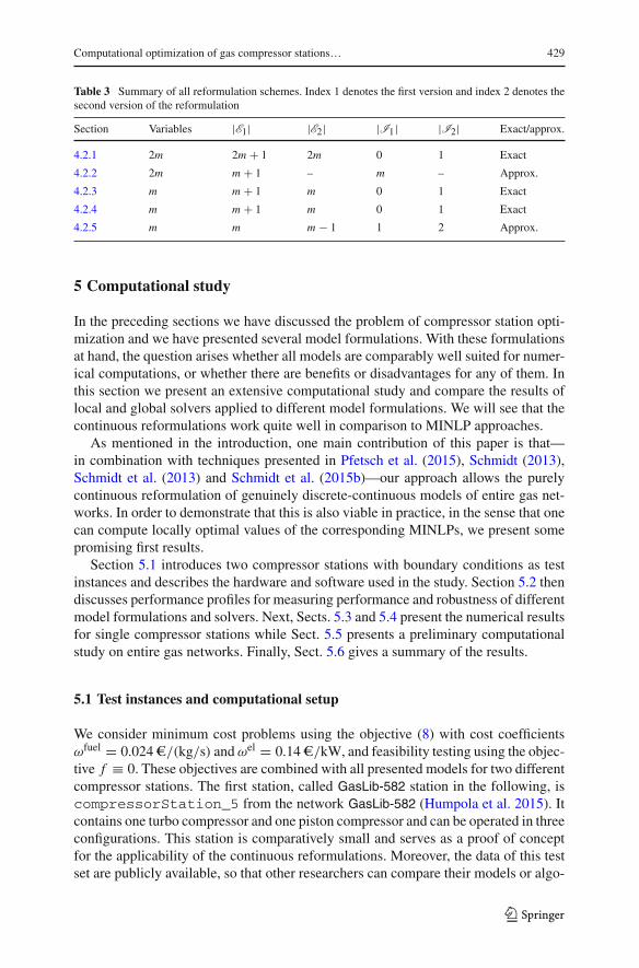
Table 3 Summary of all reformulation schemes. Index 1 denotes the first version and index 2 denotes thesecond version of the reformulation

Section Variables |E1| |E2| |I1| |I2| Exact/approx.

4.2.1 2m 2m + 1 2m 0 1 Exact

4.2.2 2m m + 1 – m – Approx.

4.2.3 m m + 1 m 0 1 Exact

4.2.4 m m + 1 m 0 1 Exact

4.2.5 m m m − 1 1 2 Approx.

5 Computational study

In the preceding sections we have discussed the problem of compressor station opti-mization and we have presented several model formulations. With these formulationsat hand, the question arises whether all models are comparably well suited for numer-ical computations, or whether there are benefits or disadvantages for any of them. Inthis section we present an extensive computational study and compare the results oflocal and global solvers applied to different model formulations. We will see that thecontinuous reformulations work quite well in comparison to MINLP approaches.

As mentioned in the introduction, one main contribution of this paper is that—in combination with techniques presented in Pfetsch et al. (2015), Schmidt (2013),Schmidt et al. (2013) and Schmidt et al. (2015b)—our approach allows the purelycontinuous reformulation of genuinely discrete-continuous models of entire gas net-works. In order to demonstrate that this is also viable in practice, in the sense that onecan compute locally optimal values of the corresponding MINLPs, we present somepromising first results.

Section 5.1 introduces two compressor stations with boundary conditions as testinstances and describes the hardware and software used in the study. Section 5.2 thendiscusses performance profiles for measuring performance and robustness of differentmodel formulations and solvers. Next, Sects. 5.3 and 5.4 present the numerical resultsfor single compressor stations while Sect. 5.5 presents a preliminary computationalstudy on entire gas networks. Finally, Sect. 5.6 gives a summary of the results.

5.1 Test instances and computational setup

We consider minimum cost problems using the objective (8) with cost coefficientsωfuel = 0.024e/(kg/s) andωel = 0.14e/kW, and feasibility testing using the objec-tive f ≡ 0. These objectives are combined with all presented models for two differentcompressor stations. The first station, called GasLib-582 station in the following, iscompressorStation_5 from the network GasLib-582 (Humpola et al. 2015). Itcontains one turbo compressor and one piston compressor and can be operated in threeconfigurations. This station is comparatively small and serves as a proof of conceptfor the applicability of the continuous reformulations. Moreover, the data of this testset are publicly available, so that other researchers can compare their models or algo-

123

430 D. Rose et al.

rithms on the same data. The second station, called HG station in the following, isa real-world compressor station of our former industry partner Open Grid Europe1

(OGE). It is one of OGE’s largest compressor stations, containing five turbo compres-sors that can be operated in 14 configurations in our model. The results on this stationillustrate the applicability of the presented models on real-world data.

The boundary values for our test instances are constructed as follows. We alwaysprescribe the in- and outflow pressures as well as the flow through the station. Forboth stations, the set of inflow pressures (in bar) is Pin = {20, 50, 80}. For everyinflow pressure pin ∈ Pin, we then construct a set of outflow pressuresPout,i (pin) ={pin + kΔpi : k = 0, . . . , 3}, i = 1, 2, where Δp1 = 13.3 bar (GasLib-582 sta-tion) and Δp2 = 20 bar (HG station). The sets of flows (in 103 Nm3h−1) are Q1 ={0, 375, 750, . . . , 2250} (GasLib-582 station) andQ2 = {0, 800, 1600, . . . , 4800} (HGstation). Thus, the complete set of boundary conditions for the GasLib-582 station is

T1 = {(pin, pout, Q0) : pin ∈ Pin, pout ∈ Pout,1(pin), Q0 ∈ Q1},

and the corresponding set for the HG station is

T2 = {(pin, pout, Q0) : pin ∈ Pin, pout ∈ Pout,2(pin), Q0 ∈ Q2}.

All values are chosen based on our experience with the technical capabilities of thestations and with typical values in gas networks. Note that the flow values for thetest sets are given as volumetric flow under normal conditions, Q0, measured in 1000normal cubicmeters per hour, as this is the standard technical unit in gas transportation.It can easily be converted to mass flow via q = cQ0ρ0, where c = 1000/3600,and ρ0 is the gas density under normal conditions. The sizes of the test sets are|T1| = |T2| = 84.

All models are implemented using the modeling language GAMS (McCarl2009) and the C++ software framework LaMaTTO++ (LaMaTTO++ 2015). Asglobal solvers for the MINLP model and its continuous (NLP type) reformula-tions we use BARON 12.3.3 (Tawarmalani and Sahinidis 2002, 2004, 2005) andSCIP 3.0 (SCIP 2015; Vigerske 2012). Additionally, we use the convex MINLPsolver KNITRO 8.1.1 (Byrd et al. 2006) as a heuristic for the nonconvex MINLPs andas NLP solver for the continuous reformulations. As local solvers for the continuousreformulations we use the interior-point code Ipopt 3.11 (Wächter and Biegler 2006)and the reduced-gradient code CONOPT4 (Drud 1994, 1995, 1996) as well as thethree MINLP solvers. The solvers are run with default settings throughout, even forsolution tolerances, as it is virtually impossible to find settings that make the resultscomparable in a strict mathematical sense.

All computations are executed on a six-core AMD Opteron Processor 2435 with2600MHz and 64GB RAM. The operating system is Debian 7.5.

1 https://www.open-grid-europe.com.

123

https://www.open-grid-europe.com


5.2 Measuring performance and robustness

To compare the computing times of different combinations of model formulations andsolvers, we use standard performance profiles (Dolan and Moré 2002). To this end, letus define the performance measure

tp,s := computing time required to solve problem p ∈ Ti by s ∈ S ,

where the set S contains all 106 combinations of model formulations and solvers:the MINLPmodel in big-M and bilinear product formulation combined with BARON,SCIP, and KNITRO (1 × 2 × 3 = 6), and each of the five continuous reformulationsin four variants (big-M and bilinear product with both pseudo NCP functions each)combined with all five solvers (5 × 4 × 5 = 100). We consider only the subsets offeasible boundary values, Fi ⊂ Ti , defined to contain those instances for which atleast one combination s ∈ S produces a feasible solution. Now the performance ratiorp,s associated with tp,s is

rp,s := tp,smin{tp,s′ : s′ ∈ S } ∈ [1,∞).

Moreover, we set rp,s = rM := max{rp′,s′ : p′ ∈ Fi , s′ ∈ Si } for those instances pthat cannot be solved by s. The logarithmically scaled performance profile is finallygiven by

ρs(τ ) := 1

|Fi | |{p ∈ Fi : log2(rp,s) ≤ τ }| ∈ [0, 1].

Finally, we remark that we use two different objective functions depending on the goalof our analysis: If we consider the performance of the solution process, we minimizecosts using objective (8). For this case we also discuss the different solution qualitiesobtained by the local solvers. If we consider the robustness of the solution process,we use the empty objective f ≡ 0 since we are only interested in whether a feasiblepoint can be found or not. In the latter case, the time used for the performance profilesthus equals the time required to find the first feasible point.

5.3 The GasLib-582 test set

The set F1 contains 48 instances of T1, hence 36 of the 84 instances are infeasible.The computing times are up to 62 s in cases where solutions are found and up to 59 s incases where a solver detects infeasibility. Some of the instances are solved in fractionsof a second. This can happen, for instance, in the preprocessing of BARON due tobound strengthening. As one would expect, the largest differences of computing timesare observed for the global solvers.

First we discuss the objective values that are obtained by the different formulationsand solvers. In theory, the global solvers BARON and SCIP should produce identical

123

432 D. Rose et al.

Table 4 GasLib-582 test set: numbers of false infeasibility reports and solver failures. Top: solver doesnot find a feasible solution with any model, bottom: no solver finds a feasible solution with any variant ofgiven model

BARON SCIP KNITRO Ipopt CONOPT4

0 7 7 7 8

MINLP EBR ABR EUR AEUR AUR

7 1 0 0 2 5

objective values whereas the local optima found by the local solvers can be larger byarbitrary amounts. However, our results show that the values of BARON and SCIPslightly differ in some cases and that all model formulations and solvers producealmost identical values on the current test set.

For every problem p ∈ F1, we compute the minimum and maximum objectivevalues f ∗

p,min and f ∗p,max as well as the maximal absolute gap g∗

p = f ∗p,max − f ∗

p,min.The minimal values f ∗

p,min range from 0 to 0.008735 (operating cost in e/s), withmaximal gaps ranging from 0 to 0.008765. The average maximal gap over p ∈ F1 isapproximately 0.0012, but most of the individual gaps are actually zero. We assumethat differing objective values are mainly caused by different numerical properties ofthe solvers. We also compared the discrete states of the compressor stations in theoptimal solutions for every instance. Different active states are found for 9 of the48 feasible instances, 3 of which have boundary values of the form Q0 = 0 andpu = pv , where the bypass mode and the closed mode are both feasible and globallyoptimal with zero cost. The remaining 6 instances have different active configurations.Thus, we have the surprising observation that on the current test set the local solversalways yield optimal values close to the global minima. A possible reason could bethat many instances admit just one feasible discrete configuration. Unfortunately wecannot find out whether this is true since it would require the huge effort of testingfeasibility for all discrete configurations.

Next, we turn to the issue of infeasibility detection. A substantial fraction of theboundary values of our test set are infeasible: 36 out of 84. In theory, if a globalsolver detects infeasibility of an instance, this is considered as an infeasibility proof.However, due to numerical inaccuracy, this is not always true in practice. To give amore detailed overview, we also list the numbers of feasible instances that are notsolved (i.e., infeasibility is reported or the solver simply fails) in Table 4. Among thesolvers, BARON clearly shows the most reliable results: for every feasible instancethere is at least one model formulation for which BARON produces a solution. Allother solvers report false infeasible results or fail in 7 or 8 cases. Surprisingly, thisis also true for the global solver SCIP. Regarding the different continuous reformu-lations, the approximate bivariate and exact univariate reformulations are solved forevery feasible instance (at least by one solver). The worst result is obtained for theMINLPmodel (7 failures). However, this result has to be carefully interpreted becausethe MINLP is handled by only 3 solvers whereas all 5 solvers can handle the con-tinuous reformulations. Within the set of reformulations, the approximate univariate

123


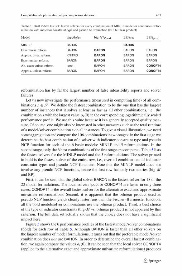
Table 5 GasLib-582 test set: fastest solvers for every combination of MINLP model or continuous refor-mulation with indicator constraint type and pseudo NCP function (BP: bilinear product)

Model big-M /φFB big-M /φprod BP/φFB BP/φprod

MINLP BARON BARON

Exact bivar. reform. BARON BARON BARON BARON

Approx. bivar. reform. KNITRO BARON BARON BARON

Exact univar. reform. BARON BARON BARON BARON

Alt. exact univar. reform. Ipopt BARON BARON CONOPT4

Approx. univar. reform. BARON BARON BARON CONOPT4

reformulation has by far the largest number of false infeasibility reports and solverfailures.

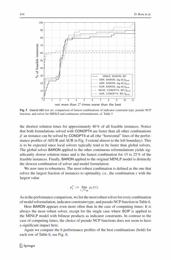
Let us now investigate the performance (measured in computing time) of all com-binations s ∈ S . We define the fastest combination to be the one that has the largestnumber of instances that it solves at least as fast as all other combinations, i.e., thecombination s with the largest value ρs(0) in the corresponding logarithmically scaledperformance profile. We use this value because it is a generally accepted quality mea-sure. Of course, onemight also be interested in othermeasures such as the total runtimeof a model/solver combination s on all instances. To give a visual illustration, we needsome aggregation and compare the 106 combinations in two stages: in the first stagewedetermine the best combination of a solver with indicator constraint type and pseudoNCP function for each of the 6 basic models: MINLP and 5 reformulations. In thesecond stage, only the 6 best combinations of the first stage are compared. Table 5 liststhe fastest solvers for the MINLP model and the 5 reformulations. The solver printedin bold is the fastest solver of the entire row, i.e., over all combinations of indicatorconstraint types and pseudo NCP functions. Note that the MINLP model does notinvolve any pseudo NCP functions, hence the first row has only two entries (big-Mand BP).

First, it can be seen that the global solver BARON is the fastest solver for 18 of the22 model formulations. The local solvers Ipopt or CONOPT4 are faster in only threecases. CONOPT4 is the overall fastest solver for the alternative exact and approximateunivariate reformulations. Second, it is apparent that the bilinear product used aspseudo NCP function yields clearly faster runs than the Fischer–Burmeister function:all the bold model/solver combinations use the bilinear product. Third, a best choiceof the type of indicator constraints (big-M vs. bilinear product) is not apparent by thiscriterion. The full data set actually shows that the choice does not have a significantimpact here.

Figure 5 shows the 6 performance profiles of the fastest model/solver combinations(bold) for each row of Table 5. Although BARON is faster than all other solvers onthe largest number of model formulations, it turns out that the preferable model/solvercombination does not use BARON. In order to determine the overall fastest combina-tion, we again compare the values ρs(0). It can be seen that the local solver CONOPT4(applied to the alternative exact and approximate univariate reformulations) produces

123

434 D. Rose et al.

Fig. 5 GasLib-582 test set: comparison of fastest combinations of indicator constraint type, pseudo NCPfunction, and solver for MINLP and continuous reformulations; cf. Table 5

the shortest solution times for approximately 40% of all feasible instances. Noticethat both formulations solved with CONOPT4 are faster than all other combinationsif an instance can be solved by CONOPT4 at all (the “horizontal” lines of the perfor-mance profiles of AEUR and AUR in Fig. 5 extend almost to the left boundary). Thisis to be expected since local solvers typically tend to be faster than global solvers.The global solver BARON applied to the other continuous reformulations yields sig-nificantly slower solution times and is the fastest combination for 15 to 25% of thefeasible instances. Finally, BARON applied to the original MINLP model is distinctlythe slowest combination of solver and model formulation.

We now turn to robustness. The most robust combination is defined as the one thatsolves the largest fraction of instances to optimality, i.e., the combination s with thelargest value

ρ∗s := lim

τ↗rMρs(τ ).

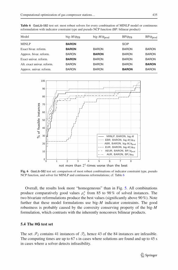
As in the performance comparison,we list themost robust solver for every combinationofmodel reformulation, indicator constraint type, and pseudoNCP function in Table 6.

Here BARON appears even more often than in the case of computing times: It isalways the most robust solver, except for the single case where SCIP is applied tothe MINLP model with bilinear products as indicator constraints. In contrast to thecase of computing times, the choice of pseudo NCP functions does not seem to havea significant impact here.

Again we compare the 6 performance profiles of the best combinations (bold) foreach row of Table 6, see Fig. 6.

123


Table 6 GasLib-582 test set: most robust solvers for every combination of MINLP model or continuousreformulation with indicator constraint type and pseudo NCP function (BP: bilinear product)


MINLP BARON SCIP


Approx. bivar. reform. BARON BARON BARON BARON

Exact univar. reform. BARON BARON BARON BARON

Alt. exact univar. reform. BARON BARON BARON BARON

Approx. univar. reform. BARON BARON BARON BARON

Fig. 6 GasLib-582 test set: comparison of most robust combinations of indicator constraint type, pseudoNCP function, and solver for MINLP and continuous reformulations; cf. Table 6

Overall, the results look more “homogeneous” than in Fig. 5. All combinationsproduce comparatively good values ρ∗

s from 85 to 98% of solved instances. Thetwo bivariate reformulations produce the best values (significantly above 90%). Notefurther that these model formulations use big-M indicator constraints. The goodrobustness is probably caused by the convexity conserving property of the big-Mformulation, which contrasts with the inherently nonconvex bilinear products.

5.4 The HG test set

The set F2 contains 41 instances of T2, hence 43 of the 84 instances are infeasible.The computing times are up to 67 s in cases where solutions are found and up to 45 sin cases where a solver detects infeasibility.

123

436 D. Rose et al.

Table 7 HG test set: numbers of false infeasibility reports and solver failures. Top: solver does not finda feasible solution with any model, bottom: no solver finds a feasible solution with any variant of givenmodel

BARON SCIP KNITRO Ipopt CONOPT4

1 3 2 8 5

MINLP EBR ABR EUR AEUR AUR

3 2 2 2 2 4

The minimal objective values (ine/s) now range from 0 to 0.069505 and the maxi-mal gaps from0 to 0.022102. The averagemaximal gap over all p ∈ F2 is significantlysmaller than for F1 at approximately 0.0006778 and most of the individual gaps areagain zero. Except for one case, the active states in the optimal solutions for a given setof boundary values are identical for all s ∈ S or consist of different sets of identicalcompressor units yielding the same objective value.2 The exceptional case is exactlythe one leading to the maximal gap. Excluding this case reduces the maximal gap overall instances by one order of magnitude.

In Table 7 we list the numbers of feasible instances for which a model could not besolved to optimality (i.e., infeasibility is reported or the solver fails). As it was the casefor the GasLib-582 station, BARON yields the smallest number of false infeasibilityreports (just one).Moreover, the choice of the class of solver (global vs. local) seems tobe more crucial than the choice of the specific model formulation: the MINLP solversreport false infeasibility in 1 to 3 cases whereas the local solvers have significantlylarger numbers of failure of 5 and 8.

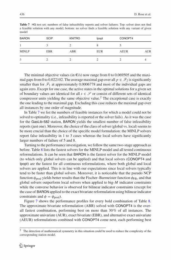
Turning to the performance investigation,we follow the same two-stage approach asbefore. Table 8 lists the fastest solvers for the MINLP model and all tested continuousreformulations. It can be seen that BARON is the fastest solver for the MINLP model(to which only global solvers can be applied) and that local solvers (CONOPT4 andIpopt) are the fastest for all continuous reformulations, where both global and localsolvers are applied. This is in line with our expectations since local solvers typicallytend to be faster than global solvers. Moreover, it is noticeable that the pseudo NCPfunction φprod yields better results than the Fischer–Burmeister function φFB, and thatglobal solvers outperform local solvers when applied to big-M indicator constraintswhile the converse behavior is observed for bilinear indicator constraints (except forthe case of BARON applied to the exact bivariate reformulation using bilinear indicatorconstraints and φ = φprod).

Figure 7 shows the performance profiles for every bold combination of Table 8.The approximate bivariate reformulation (ABR) solved with CONOPT4 is the over-all fastest combination, performing best on more than 30% of all instances. Theapproximate univariate (AUR), exact bivariate (EBR), and alternative exact univariate(AEUR) reformulations combined with CONOPT4 come next, each performing best

2 The detection of mathematical symmetry in this situation could be used to reduce the complexity of thecorresponding station model.

123


Table 8 HG test set: fastest solvers for every combination of MINLP model or continuous reformulationwith indicator constraint type and pseudo NCP function (BP: bilinear product)


MINLP KNITRO BARON

Exact bivar. reform. BARON CONOPT4 CONOPT4 BARON

Approx. bivar. reform. BARON CONOPT4 Ipopt Ipopt

Exact univar. reform. KNITRO BARON Ipopt Ipopt

Alt. exact univar. reform. Ipopt SCIP Ipopt CONOPT4

Approx. univar. reform. BARON SCIP Ipopt CONOPT4

Fig. 7 HG test set: comparison of fastest combinations of indicator constraint type, pseudo NCP function,and solver for MINLP and continuous reformulations; cf. Table 8

on roughly 20% of all instances. Since the approximate univariate formulation showsbetter results than EBR and AEUR for small values τ > 0, we may summarize thatthe approximate reformulations (combined with φ = φprod) tend to be the fastest com-binations. A possible reason might be that for local solvers the enlarged feasible set ispreferable to the feasible sets of lower dimension of the exact reformulations. In addi-tion, the overall preferable approximate bivariate scheme is also the “most regular”formulation with respect to the LICQ (cf. Sect. 4.2). Finally we note that in terms ofsolution times both the exact univariate reformulation and the MINLP model cannotcompete with the other reformulations.

Regarding robustness, the situation changes completely. We list the most robustsolver (the one with largest ρ∗

s ) for every combination of model reformulation, indi-cator constraint type, and pseudo NCP function in Table 9. For the original MINLP

123

438 D. Rose et al.

Table 9 HG test set: most robust solvers for every combination of MINLP model or continuous reformu-lation with indicator constraint type and pseudo NCP function (BP: bilinear product)


MINLP KNITRO SCIP


Approx. bivar. reform. BARON BARON BARON BARON

Exact univar. reform. BARON SCIP BARON BARON

Alt. exact univar. reform. BARON SCIP BARON BARON

Approx. univar. reform. BARON SCIP KNITRO BARON

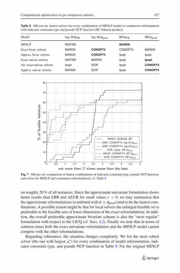
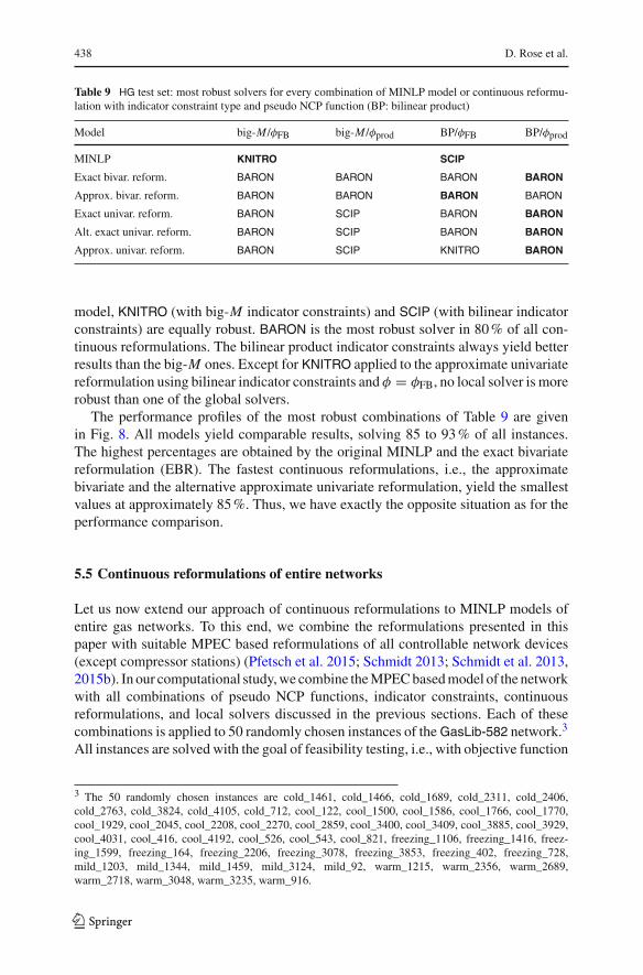
model, KNITRO (with big-M indicator constraints) and SCIP (with bilinear indicatorconstraints) are equally robust. BARON is the most robust solver in 80% of all con-tinuous reformulations. The bilinear product indicator constraints always yield betterresults than the big-M ones. Except for KNITRO applied to the approximate univariatereformulation using bilinear indicator constraints and φ = φFB, no local solver is morerobust than one of the global solvers.

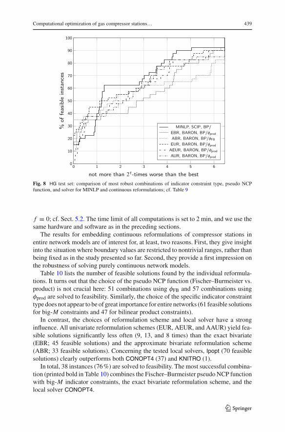
The performance profiles of the most robust combinations of Table 9 are givenin Fig. 8. All models yield comparable results, solving 85 to 93% of all instances.The highest percentages are obtained by the original MINLP and the exact bivariatereformulation (EBR). The fastest continuous reformulations, i.e., the approximatebivariate and the alternative approximate univariate reformulation, yield the smallestvalues at approximately 85%. Thus, we have exactly the opposite situation as for theperformance comparison.

5.5 Continuous reformulations of entire networks

Let us now extend our approach of continuous reformulations to MINLP models ofentire gas networks. To this end, we combine the reformulations presented in thispaper with suitable MPEC based reformulations of all controllable network devices(except compressor stations) (Pfetsch et al. 2015; Schmidt 2013; Schmidt et al. 2013,2015b). In our computational study,we combine theMPECbasedmodel of the networkwith all combinations of pseudo NCP functions, indicator constraints, continuousreformulations, and local solvers discussed in the previous sections. Each of thesecombinations is applied to 50 randomly chosen instances of theGasLib-582 network.3

All instances are solved with the goal of feasibility testing, i.e., with objective function

3 The 50 randomly chosen instances are cold_1461, cold_1466, cold_1689, cold_2311, cold_2406,cold_2763, cold_3824, cold_4105, cold_712, cool_122, cool_1500, cool_1586, cool_1766, cool_1770,cool_1929, cool_2045, cool_2208, cool_2270, cool_2859, cool_3400, cool_3409, cool_3885, cool_3929,cool_4031, cool_416, cool_4192, cool_526, cool_543, cool_821, freezing_1106, freezing_1416, freez-ing_1599, freezing_164, freezing_2206, freezing_3078, freezing_3853, freezing_402, freezing_728,mild_1203, mild_1344, mild_1459, mild_3124, mild_92, warm_1215, warm_2356, warm_2689,warm_2718, warm_3048, warm_3235, warm_916.

123


Fig. 8 HG test set: comparison of most robust combinations of indicator constraint type, pseudo NCPfunction, and solver for MINLP and continuous reformulations; cf. Table 9

f ≡ 0; cf. Sect. 5.2. The time limit of all computations is set to 2 min, and we use thesame hardware and software as in the preceding sections.

The results for embedding continuous reformulations of compressor stations inentire network models are of interest for, at least, two reasons. First, they give insightinto the situation where boundary values are restricted to nontrivial ranges, rather thanbeing fixed as in the study presented so far. Second, they provide a first impression onthe robustness of solving purely continuous network models.

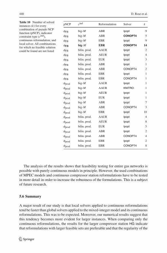
Table 10 lists the number of feasible solutions found by the individual reformula-tions. It turns out that the choice of the pseudo NCP function (Fischer–Burmeister vs.product) is not crucial here: 51 combinations using φFB and 57 combinations usingφprod are solved to feasibility. Similarly, the choice of the specific indicator constrainttype does not appear to be of great importance for entire networks (61 feasible solutionsfor big-M constraints and 47 for bilinear product constraints).

In contrast, the choices of reformulation scheme and local solver have a stronginfluence. All univariate reformulation schemes (EUR, AEUR, and AAUR) yield fea-sible solutions significantly less often (9, 13, and 8 times) than the exact bivariate(EBR; 45 feasible solutions) and the approximate bivariate reformulation scheme(ABR; 33 feasible solutions). Concerning the tested local solvers, Ipopt (70 feasiblesolutions) clearly outperforms both CONOPT4 (37) and KNITRO (1).

In total, 38 instances (76%) are solved to feasibility. The most successful combina-tion (printed bold in Table 10) combines the Fischer–Burmeister pseudo NCP functionwith big-M indicator constraints, the exact bivariate reformulation scheme, and thelocal solver CONOPT4.

123

440 D. Rose et al.

Table 10 Number of solvedinstances (k) for everycombination of pseudo NCPfunction (pNCP), indicatorconstraint type (cind),continuous reformulation, andlocal solver. All combinationsfor which no feasible solutioncould be found are not listed

pNCP cind Reformulation Solver k

φFB big-M ABR Ipopt 9

φFB big-M ABR CONOPT4 5

φFB big-M EBR Ipopt 9

φFB big-M EBR CONOPT4 14

φFB bilin. prod. AAUR Ipopt 2

φFB bilin. prod. AEUR Ipopt 4

φFB bilin. prod. EUR Ipopt 3

φFB bilin. prod. ABR Ipopt 1

φFB bilin. prod. ABR CONOPT4 2

φFB bilin. prod. EBR Ipopt 1

φFB bilin. prod. EBR CONOPT4 1

φprod big-M AAUR Ipopt 1

φprod big-M AAUR KNITRO 1

φprod big-M AEUR Ipopt 1

φprod big-M EUR Ipopt 1

φprod big-M ABR Ipopt 7

φprod big-M ABR CONOPT4 3

φprod big-M EBR Ipopt 10

φprod bilin. prod. AAUR Ipopt 4

φprod bilin. prod. AEUR Ipopt 8

φprod bilin. prod. EUR Ipopt 5

φprod bilin. prod. ABR Ipopt 2

φprod bilin. prod. ABR CONOPT4 4

φprod bilin. prod. EBR Ipopt 2

φprod bilin. prod. EBR CONOPT4 8

The analysis of the results shows that feasibility testing for entire gas networks ispossible with purely continuous models in principle. However, the used combinationsof MPEC models and continuous compressor station reformulations have to be testedin more detail in order to increase the robustness of the formulations. This is a subjectof future research.

5.6 Summary

A major result of our study is that local solvers applied to continuous reformulationstend be faster than global solvers applied to themixed-integermodel and its continuousreformulations. This was to be expected. Moreover, our numerical results suggest thatthis tendency becomes more evident for larger instances. When comparing only thecontinuous reformulations, the results for the larger compressor station HG indicatethat reformulations with larger feasible sets are preferable and that the regularity of the

123


formulation has a strong impact on the performance of the solution process. (Recallthat the “most regular” approximate bivariate reformulation yields the best solutiontimes on the large test set.) Finally, global solvers (especially BARON) produce morerobust results, independent of the choice of model formulation.

Our results also indicate which types of indicator constraints work well with a givensolver. Especially for larger instances, global solvers tend to be faster on big-M for-mulations while local solvers perform better with bilinear products. A probable reasonfor this is that the behavior of global solvers is stronger influenced by nonconvexitythan it is the case for local solvers. The situation changes with regard to robustnessof the solution process, where the bilinear indicator constraint is clearly preferable tothe big-M formulation.

A second observation concerns the preferable type of pseudo NCP functions:The product formulation φprod distinctly outperforms Fischer–Burmeister functions.Although the latter are quite prominent in the literature, the simple formulation usingproducts usually produces faster and more robust formulations in practice.

Finally we can state that, for the models considered in this paper, there are nosignificant drawbacks concerning the quality of solutions when local solvers are used.These results are perhaps not entirely surprising for the considered class of real-worldproblems. However, no systematic study exists in the literature up to now.

The tendencies observed above might change when fixed boundary values arereplaced with nontrivial feasible ranges. This happens, e.g., when the tested con-tinuous reformulations of compressor stations are used in continuous models of entirenetworks. As expected, the resulting instances are hard, but we have seen in Sect. 5.5that in principle they can be solved by local solvers. Nevertheless, more extensivetesting of model combinations and possibly the development of further model variantsare required in order to obtain more robust formulations. Both issues are subjects offuture research.

6 Conclusion

In this article we have presented MINLP and GDP models for cost optimization andfeasibility testing of gas compressor stations. Moreover, we have considered differenttypes of continuous reformulation techniques from the literature and applied them tothe application problem. Our computational study shows that local solvers applied tocontinuous reformulations can be used to replace MINLP formulations that can onlybe tackled by global solvers. The continuous reformulations yield comparably robustresults, optimal values of almost the same quality on our test set, and tend to be solvablewithin shorter solution times. Together with the techniques developed in Pfetsch et al.(2015), Schmidt (2013), Schmidt et al. (2013), and Schmidt et al. (2015b), this articleprovides a complete continuous reformulation of the discrete-continuous problem ofstationary gas transport optimization. Additionally, first promising numerical resultson a large-scale network underpin the practical usability of continuous reformulationsfor entire networks.

However, somequestions remain open.Wehave considered a stationary and isother-mal variant of the problem of compressor station optimization. Since including gas

123

442 D. Rose et al.

temperature as a dynamic variable mainly leads to increased nonlinearity and noncon-vexity in the model, we expect that continuous reformulations tend to be even morefavorable for these models. In contrast, the consideration of the transient case will alsoincrease the amount of discrete aspects so that it is unclear which formulation will befavorable in this case. Finally, more extensive testing of suitable continuous modelsfor entire networks is a subject of future research.

Acknowledgments This work has been supported by the German Federal Ministry of Economics andTechnology owing to a decision of the German Bundestag. The responsibility for the content of this pub-lication lies with the authors. This research has been conducted as part of the Energie Campus Nürnbergand supported by funding through the “Aufbruch Bayern (Bavaria on the move)” initiative of the state ofBavaria. We are also very grateful to Benjamin Hiller for his comments on an earlier version of this paper.Finally, we thank our former industry partner Open Grid Europe GmbH for their support.

Compliance with ethical standards

Conflicts of interest The authors declare that they have no conflict of interest

Human and Animal Participants This article does not contain any studies with human or animal subjects

Open Access This article is distributed under the terms of the Creative Commons Attribution 4.0 Interna-tional License (http://creativecommons.org/licenses/by/4.0/), which permits unrestricted use, distribution,and reproduction in any medium, provided you give appropriate credit to the original author(s) and thesource, provide a link to the Creative Commons license, and indicate if changes were made.

References

Banda MK, Herty M (2008) Multiscale modeling for gas flow in pipe networks. Math Methods Appl Sci31:915–936. doi:10.1002/mma.948

Banda MK, Herty M, Klar A (2006) Gas flow in pipeline networks. Netw Heterog Media 1(1):41–56.doi:10.3934/nhm.2006.1.41

Baumrucker BT, Renfro JG, Biegler LT (2008) MPEC problem formulations and solution strategies withchemical engineering applications. Comput Chem Eng 32:2903–2913. doi:10.1016/j.compchemeng.2008.02.010

BockHG,Kostina E, PhuHX, Rannacher R (eds) (2005)Modeling, simulation and optimization of complexprocesses. Springer, Berlin

Brouwer J, Gasser I, Herty M (2011) Gas pipeline models revisited: model hierarchies, nonisothermalmodels, and simulations of networks. Multiscale Model Simul 9(2):601–623. doi:10.1137/100813580

Byrd RH, Nocedal J, Waltz RA (2006) KNITRO: An integrated package for nonlinear optimization. In:Large scale nonlinear optimization, Springer Verlag, pp 35–59. doi:10.1007/0-387-30065-1_4

Carter RG (1996) Compressor station optimization: computational accuracy and speed. In: 28th annualmeeting, Pipeline Simulation Interest Group. Paper 9605

Carter RG (1998) Pipeline optimization: dynamic programming after 30 years. In: PSIG 30th annual meet-ing, Denver, Colorado. Paper 9803

Carter RG, Schroeder DW, Harbick TD (1994) Some causes and effects of discontinuities in modeling andoptimizing gas transmission networks. Tech. rep, Stoner Associates, Carlisle, PA, USA

Cobos-Zaleta D, Ríos-Mercado RZ (2002) AMINLP model for a problem of minimizing fuel consumptiononnatural gas pipeline networks. In: Proceedings ofXILatin-Ibero-American conference onoperationsresearch, pp 1–9. Paper A48–01

Dolan ED, Moré JJ (2002) Benchmarking optimization software with performance profiles. Math Program91(2):201–213. doi:10.1007/s101070100263

Domschke P, Geißler B, Kolb O, Lang J, Martin A, Morsi A (2011) Combination of nonlinear and linearoptimization of transient gas networks. INFORMS J Comput 23(4):605–617. doi:10.1287/ijoc.1100.0429

123

http://creativecommons.org/licenses/by/4.0/

http://dx.doi.org/10.1002/mma.948

http://dx.doi.org/10.3934/nhm.2006.1.41

http://dx.doi.org/10.1016/j.compchemeng.2008.02.010


http://dx.doi.org/10.1137/100813580

http://dx.doi.org/10.1007/0-387-30065-1_4

http://dx.doi.org/10.1007/s101070100263

http://dx.doi.org/10.1287/ijoc.1100.0429

http://dx.doi.org/10.1287/ijoc.1100.0429


Drud AS (1994) CONOPT—a large-scale GRG code. INFORMS J Comput 6(2):207–216. doi:10.1287/ijoc.6.2.207

DrudAS (1995) CONOPT: a system for large scale nonlinear optimization, tutorial for CONOPT subroutinelibrary. Tech. rep, ARKI Consulting and Development A/S, Bagsvaerd, Denmark

Drud AS (1996) CONOPT: a system for large scale nonlinear optimization, reference manual for CONOPTsubroutine library. Tech. rep, ARKI Consulting and Development A/S, Bagsvaerd, Denmark

Ehrhardt K, Steinbach MC (2004) KKT systems in operative planning for gas distribution networks. ProcAppl Math Mech 4(1):606–607. doi:10.1002/pamm.200410284

Ehrhardt K, Steinbach MC (2005) Nonlinear optimization in gas networks. In: Bock et al. (eds) Model-ing, simulation and optimization of complex processes. Springer, Berlin, pp. 139–148. doi:10.1007/3-540-27170-8_11

Eurostat (2013) Gross inland energy consumption by fuel type. http://epp.eurostat.ec.europa.eu/tgm/refreshTableAction.do?tab=table&plugin=1&pcode=tsdcc320&language=en. Downloaded on 2 Oct2015

Fischer A (1992) A special Newton-type optimization method. Optimization 24(3–4):269–284. doi:10.1080/02331939208843795

Geißler B, Morsi A, Schewe L (2013) A new algorithm for MINLP applied to gas transport energy costminimization. In: Jünger M, Reinelt G (eds) Facets of combinatorial optimization, Springer, BerlinHeidelberg, pp 321–353. doi:10.1007/978-3-642-38189-8_14

Geißler B (2011) Towards globally optimal solutions forMINLPs by discretization techniques with applica-tions in gas network optimization. Ph.D. thesis, Friedrich-Alexander Universität Erlangen-Nürnberg,Germany

Grossmann IE (2002) Review of nonlinear mixed-integer and disjunctive programming techniques. OptimEng 3(3):227–252. doi:10.1023/A:1021039126272 Special issue on mixed-integer programming andits applications to engineering

Gugat M, Hante FM, Hirsch-Dick M, Leugering G (2015) Stationary states in gas networks. Netw HeterogMedia 10(2):295–320. doi:10.3934/nhm.2015.10.295

Humpola J, Joormann I, Oucherif D, Pfetsch ME, Schewe L, Schmidt M, Schwarz R (2015) GasLib—alibrary of gas network instances. http://www.optimization-online.org/DB_HTML/2015/11/5216.html

Jenícek T, Králik J (1995) Optimized control of generalized compressor station. In: PSIG annual meetingKoch T, Hiller B, PfetschME, Schewe L (eds) (2015) Evaluating gas network capacities. SIAM-MOS series

on optimization. SIAM. doi:10.1137/1.9781611973693Kraemer K, Kossack S, Marquardt W (2007) An efficient solution method for the MINLP optimization

of chemical processes. In: V Plesu, PS Agachi (eds) 17th European symposium on computer aidedprocess engineering, computer aided chemical engineering, vol. 24, Elsevier, pp 105–110. doi:10.1016/S1570-7946(07)80041-1

Kraemer K, Marquardt W (2010) Continuous reformulation of MINLP problems. In: M Diehl, F Glineur,E Jarlebring, W Michiels (eds) Recent advances in optimization and its applications in engineering,Springer, Berlin Heidelberg, pp 83–92. doi:10.1007/978-3-642-12598-0_8

Králik J (1993) Compressor stations in SIMONE. In: Proceedings of 2nd international workshop SIMONEon innovative approaches to modeling and optimal control of large scale pipeline networks, Prague,pp 93–117

LaMaTTO++ (2015) A framework for modeling and solving mixed-integer nonlinear programming prob-lems on networks. http://www.mso.math.fau.de/edom/projects/lamatto.html

Luo ZQ, Pang JS, Ralph D (1996) Mathematical programs with equilibrium constraints. Cambridge Uni-versity Press, Cambridge

Martin A, Möller M (2005) Cutting planes for the optimization of gas networks. In: Bock et al. (eds)Modeling, simulation and optimization of complex processes. Springer, Berlin, pp. 307–329. doi:10.1007/3-540-27170-8_24

Martin A, Mahlke D, Moritz S (2007) A simulated annealing algorithm for transient optimization in gasnetworks. Math Methods Oper Res 66(1):99–115. doi:10.1007/s00186-006-0142-9

Martin A, Möller M, Moritz S (2006) Mixed integer models for the stationary case of gas network opti-mization. Math Program 105(2–3):563–582. doi:10.1007/s10107-005-0665-5

McCarl BA (2009) GAMS user guide. VERSION 23.0Odom FM, Muster GL (2009) Tutorial on modeling of gas turbine driven centrifugal compressors. Tech.

Rep. 09A4, Pipeline Simulation Interest Group

123

http://dx.doi.org/10.1287/ijoc.6.2.207

http://dx.doi.org/10.1287/ijoc.6.2.207

http://dx.doi.org/10.1002/pamm.200410284

http://dx.doi.org/10.1007/3-540-27170-8_11

http://dx.doi.org/10.1007/3-540-27170-8_11

http://epp.eurostat.ec.europa.eu/tgm/refreshTableAction.do?tab=table&plugin=1&pcode=tsdcc320&language=en

http://epp.eurostat.ec.europa.eu/tgm/refreshTableAction.do?tab=table&plugin=1&pcode=tsdcc320&language=en

http://dx.doi.org/10.1080/02331939208843795

http://dx.doi.org/10.1080/02331939208843795

http://dx.doi.org/10.1007/978-3-642-38189-8_14

http://dx.doi.org/10.1023/A:1021039126272

http://dx.doi.org/10.3934/nhm.2015.10.295

http://www.optimization-online.org/DB_HTML/2015/11/5216.html

http://dx.doi.org/10.1137/1.9781611973693

http://dx.doi.org/10.1016/S1570-7946(07)80041-1

http://dx.doi.org/10.1016/S1570-7946(07)80041-1

http://dx.doi.org/10.1007/978-3-642-12598-0_8

http://www.mso.math.fau.de/edom/projects/lamatto.html

http://dx.doi.org/10.1007/3-540-27170-8_24

http://dx.doi.org/10.1007/3-540-27170-8_24

http://dx.doi.org/10.1007/s00186-006-0142-9

http://dx.doi.org/10.1007/s10107-005-0665-5

444 D. Rose et al.

Osiadacz A (1980) Nonlinear programming applied to the optimum control of a gas compressor station. IntJ Numer Methods Eng 15(9):1287–1301. doi:10.1002/nme.1620150902

Pfetsch ME, Fügenschuh A, Geißler B, Geißler N, Gollmer R, Hiller B, Humpola J, Koch T, Lehmann T,Martin A,Morsi A, Rövekamp J, Schewe L, SchmidtM, Schultz R, Schwarz R, Schweiger J, Stangl C,SteinbachMC, Vigerske S,Willert BM (2015) Validation of nominations in gas network optimization:models, methods, and solutions. Optim Methods Softw 30(1):15–53. doi:10.1080/10556788.2014.888426

Raman R, Grossmann IE (1994) Modeling and computational techniques for logic based integer program-ming. Comput Chem Eng 18(7):563–578. doi:10.1016/0098-1354(93)E0010-7

Schewe L, Koch T, Martin A, Pfetsch ME (2015) Mathematical optimization for evaluating gas networkcapacities. In: Koch et al. (eds) Evaluating gas network capacities, chap. 5, pp. 87–102. doi:10.1137/1.9781611973693.ch5

Schmidt M (2013) A generic interior-point framework for nonsmooth and complementarity constrainednonlinear optimization. Ph.D. thesis, Gottfried Wilhelm Leibniz Universität Hannover

Schmidt M, Steinbach MC, Willert BM (2013) A primal heuristic for nonsmooth mixed integer nonlinearoptimization. In: M Jünger, G Reinelt (eds) Facets of combinatorial optimization, Springer, Berlin,Heidelberg, pp 295–320. doi:10.1007/978-3-642-38189-8_13

SchmidtM, SteinbachMC,Willert BM (2015a)High detail stationary optimizationmodels for gas networks:validation and results. Optim Eng. doi:10.1007/s11081-015-9300-3

Schmidt M, Steinbach MC, Willert BM (2015b) An MPEC based heuristic. In: Koch et al. (eds) Evaluatinggas network capacities, chap. 9, pp. 163–179. doi:10.1137/1.9781611973693.ch9

SchmidtM, SteinbachMC,Willert BM(2015c)High detail stationary optimizationmodels for gas networks.Optim Eng 16(1):131–164. doi:10.1007/s11081-014-9246-x

SCIP (2015) Solving constraint integer programs. http://scip.zib.de/Stein O, Oldenburg J, Marquardt W (2004) Continuous reformulations of discrete-continuous optimization

problems. Comput Chem Eng 28(10):1951–1966. doi:10.1016/j.compchemeng.2004.03.011Steinbach MC (2007) On PDE solution in transient optimization of gas networks. J Comput Appl Math

203(2):345–361. doi:10.1016/j.cam.2006.04.018Sun D, Qi L (1999) On NCP-functions. Comput. Optim. Appl. 13(1–3):201–220. doi:10.1023/A:

1008669226453 Computational Optimization—a Tribute to Olvi Mangasarian, Part IITawarmalani M, Sahinidis NV (2002) Convexification and global optimization in continuous and mixed-

integer nonlinear programming: theory software, and applications. Kluwer Academic Publishers,Algorithms

Tawarmalani M, Sahinidis NV (2004) Global optimization of mixed-integer nonlinear programs: a theoret-ical and computational study. Math Program 99(3):563–591. doi:10.1007/s10107-003-0467-6

Tawarmalani M, Sahinidis NV (2005) A polyhedral branch-and-cut approach to global optimization. MathProgram 103(2):225–249. doi:10.1007/s10107-005-0581-8

Vigerske S (2012) Decomposition in multistage stochastic programming and a constraint integer program-ming approach tomixed-integer nonlinear programming. Ph.D. thesis, Humboldt-Universität zuBerlin

Wächter A, Biegler LT (2006) On the implementation of an interior-point filter line-search algorithm forlarge-scale nonlinear programming. Math Program 106(1):25–57. doi:10.1007/s10107-004-0559-y

Wong PJ, Larson RE (1968a) Optimization of natural-gas pipeline systems via dynamic programming.IEEE Trans Autom Control 13:475–481. doi:10.1109/TAC.1968.1098990

Wong PJ, Larson RE (1968b) Optimization of tree-structured natural-gas transmission networks. J MathAnal Appl 24:613–626. doi:10.1016/0022-247X(68)90014-0

Wright S, Somani M, Ditzel C (1998) Compressor station optimization. In: PSIG 30th annual meeting,Denver, Colorado. Paper 9805

Ye JJ, Zhu DL (1995) Optimality conditions for bilevel programming problems. Optimization 33:9–27.doi:10.1080/02331939508844060

123

http://dx.doi.org/10.1002/nme.1620150902

http://dx.doi.org/10.1080/10556788.2014.888426

http://dx.doi.org/10.1080/10556788.2014.888426

http://dx.doi.org/10.1016/0098-1354(93)E0010-7

http://dx.doi.org/10.1137/1.9781611973693.ch5

http://dx.doi.org/10.1137/1.9781611973693.ch5

http://dx.doi.org/10.1007/978-3-642-38189-8_13

http://dx.doi.org/10.1007/s11081-015-9300-3

http://dx.doi.org/10.1137/1.9781611973693.ch9

http://dx.doi.org/10.1007/s11081-014-9246-x

http://scip.zib.de/


http://dx.doi.org/10.1016/j.cam.2006.04.018

http://dx.doi.org/10.1023/A:1008669226453

http://dx.doi.org/10.1023/A:1008669226453

http://dx.doi.org/10.1007/s10107-003-0467-6

http://dx.doi.org/10.1007/s10107-005-0581-8

http://dx.doi.org/10.1007/s10107-004-0559-y

http://dx.doi.org/10.1109/TAC.1968.1098990

http://dx.doi.org/10.1016/0022-247X(68)90014-0

http://dx.doi.org/10.1080/02331939508844060

Computational optimization of gas compressor stations ...

Documents

Transcript of Computational optimization of gas compressor stations ...