
Computational Models of Episodic Memory · PDF file2 Computationalmodelsofepisodicmemory 1....
72
Running Head: Computational models of episodic memory Computational Models of Episodic Memory Kenneth A. Norman, Greg Detre, & Sean M. Polyn To appear in R. Sun (Ed.), The Cambridge Handbook of Computational Cognitive Modeling August 27, 2006
-
Upload
vuongthien -
Category
Documents
-
view
216 -
download
1
Transcript of Computational Models of Episodic Memory · PDF file2 Computationalmodelsofepisodicmemory 1....

Running Head: Computational models of episodic memory
Computational Models of Episodic Memory
Kenneth A. Norman, Greg Detre, & Sean M. Polyn
To appear in R. Sun (Ed.), The Cambridge Handbook of Computational Cognitive Modeling
August 27, 2006
2 Computational models of episodic memory
1. Introduction
The term episodic memory refers to our ability to recall previously experienced events, and to
recognize things as having been encountered previously. Over the past several decades, research
on the neural basis of episodic memory has increasingly come to focus on three structures:
• The hippocampus supports recall of specific details from previously experienced events (for
neuroimaging evidence, see, e.g., Davachi, Mitchell, & Wagner, 2003; Ranganath, Yoneli-
nas, Cohen, Dy, Tom, & D’Esposito, 2003; Eldridge, Knowlton, Furmanski, Bookheimer, &
Engel, 2000; Dobbins, Rice, Wagner, & Schacter, 2003; for a review of relevant lesion data,
see Aggleton & Brown, 1999).
• Perirhinal cortex computes a scalar familiarity signal that discriminates between studied
and nonstudied items (for neuroimaging evidence, see, e.g., Gonsalves, Kahn, Curran, Nor-
man, & Wagner, 2005; Henson, Cansino, Herron, Robb, & Rugg, 2003; Brozinsky, Yoneli-
nas, Kroll, & Ranganath, 2005; for neurophysiological evidence, see, e.g., Li, Miller, &
Desimone, 1993; Xiang & Brown, 1998; for evidence that perirhinal cortex can support near-
normal levels of familiarity-based recognition on its own, after focal hippocampal damage,
see, e.g., Yonelinas, Kroll, Quamme, Lazzara, Sauve, Widaman, & Knight, 2002; Fortin,
Wright, & Eichenbaum, 2004; but see, e.g., Manns, Hopkins, Reed, Kitchener, & Squire,
2003 for an opposing viewpoint).
• Prefrontal cortex plays a critical role in memory targeting: In situations where the bottom-up
retrieval cue is not sufficiently specific to trigger activation of memory traces in the medial
temporal lobe, prefrontal cortex acts to flesh out the retrieval cue, by actively maintaining ad-
ditional information that specifies the to-be-retrieved episode (for reviews of how prefrontal
cortex contributes to episodic memory, see Simons & Spiers, 2003; Fletcher & Henson,
2001; Shimamura, 1994; Schacter, 1987).
Norman, Detre, & Polyn 3
While there is general agreement about the roles of the three structures mentioned above, there
is less agreement about how (mechanistically) these structures enact the roles specified above. This
chapter reviews two kinds of models: biologically-based models that are meant to address how
the neural structures mentioned above contribute to recognition and recall; and abstract models
that try to describe the mental algorithms that support recognition and recall judgments, without
specifically addressing how these algorithms might be implemented in the brain.
Weight-based vs. activation-based memory mechanisms
Within the realm of biologically-based episodic memory models, one can make a distinction
between weight-based and activation-based memory mechanisms (O’Reilly & Munakata, 2000).
Weight-based memory mechanisms support recognition and recall by making lasting changes to
synaptic weights at study. Activation-based memory mechanisms support recognition and recall of
an item by actively maintaining the pattern of neural activity elicited by the item during the study
phase. Activation-based memory mechanisms can support recognition and recall after short delays.
However, our ability to recognize and recall stimuli after longer delays depends on changes to
synaptic weights. This chapter primarily focuses on weight-based memory mechanisms, although
Section 4 discusses interactions between weight-based and activation-based memory mechanisms.
Outline
Section 2 of the chapter provides an overview of biological models of episodic memory, with
a special focus on the Complementary Learning Systems model (McClelland, McNaughton, &
O’Reilly, 1995; Norman & O’Reilly, 2003). Section 3 reviews abstract models of episodic mem-
ory. Section 4 discusses how both abstract and biological models have been extended to address
temporal context memory: our ability to focus retrieval on a particular time period, to the exclusion
of others. This section starts by describing the abstract Temporal Context Model (TCM) devel-
oped by Howard and Kahana (2002). The remainder of Section 4 discusses how temporal context

4 Computational models of episodic memory
memory can be instantiated in neural systems.
2. Biologically-based models of episodic memory
The first part of this section reviews the Complementary Learning Systems (CLS) model (Mc-
Clelland et al., 1995) and how it has been applied to understanding hippocampal and neocortical
contributions to episodic memory (Norman & O’Reilly, 2003). Section 2.2 discusses some alter-
native views of how neocortex contributes to episodic memory.
2.1. The Complementary Learning Systems model
The CLS model incorporates several widely-held ideas about the division of labor between hip-
pocampus and neocortex that have been developed over many years by many different researchers
(e.g., Scoville & Milner, 1957; Marr, 1971; Grossberg, 1976; O’Keefe & Nadel, 1978; Teyler &
Discenna, 1986; McNaughton & Morris, 1987; Sherry & Schacter, 1987; Rolls, 1989; Suther-
land & Rudy, 1989; Squire, 1992; Eichenbaum, Otto, & Cohen, 1994; Treves & Rolls, 1994;
Burgess & O’Keefe, 1996; Wu, Baxter, & Levy, 1996; Moll & Miikkulainen, 1997; Hasselmo &
Wyble, 1997; Aggleton & Brown, 1999; Yonelinas, 2002; Becker, 2005). According to the CLS
model, neocortex forms the substrate of our internal model of the structure of the environment. In
contrast, hippocampus is specialized for rapidly and automatically memorizing patterns of cortical
activity, so they can be recalled later (based on partial cues). The model posits that neocortex learns
incrementally; each training trial results in relatively small adaptive changes in synaptic weights.
These small changes allow cortex to gradually adjust its internal model of the environment in re-
sponse to new information. The other key property of neocortex (according to the model) is that
it assigns similar (overlapping) representations to similar stimuli. Use of overlapping representa-
tions allows cortex to represent the shared structure of events, and therefore makes it possible for
cortex to generalize to novel stimuli based on their similarity to previously experienced stimuli.
Norman, Detre, & Polyn 5
In contrast, the model posits that hippocampus assigns distinct, pattern separated representations
to stimuli, regardless of their similarity. This property allows hippocampus to rapidly memorize
arbitrary patterns of cortical activity without suffering unacceptably high (catastrophic) levels of
interference.
Applying CLS to episodic memory
CLS was originally formulated as a set of high-level principles for understanding hippocampal
and cortical contributions to memory. More recently, Norman and O’Reilly (2003) implemented
hippocampal and cortical networks that adhere to CLS principles, and used the models to simulate
episodic memory data. Learning was implemented in these simulations using a simple Hebbian
rule, called instar learning by Grossberg (1976) and Conditional Principal Components Analysis
(CPCA) Hebbian learning by O’Reilly and Munakata (2000):
∆wij = εyj(xi − wij) (1)
In this equation, xi is the activation of sending unit i, yj is the activation of receiving unit j,
wij is the strength of the connection between i and j, and ε is the learning rate parameter. This
rule has the effect of strengthening connections between active sending and receiving neurons, and
weakening connections between active receiving neurons and inactive sending neurons.
In both the hippocampal and cortical networks, to-be-memorized items are represented by pat-
terns of excitatory activity that are distributed across multiple units (simulated neurons) in the
network. Excitatory activity spreads from unit to unit via positive-valued synaptic weights. The
overall level of excitatory activity in the network is controlled by a feedback inhibition mechanism
that samples the amount of excitatory activity in a particular subregion of the model, and sends
back a proportional amount of inhibition (O’Reilly & Munakata, 2000).
The CLS model instantiates the idea (mentioned in the Introduction) that hippocampus con-
tributes to recognition memory by recalling specific studied details, and that cortex contributes
6 Computational models of episodic memory
Input
EC_in
DG
CA3 CA1
EC_out
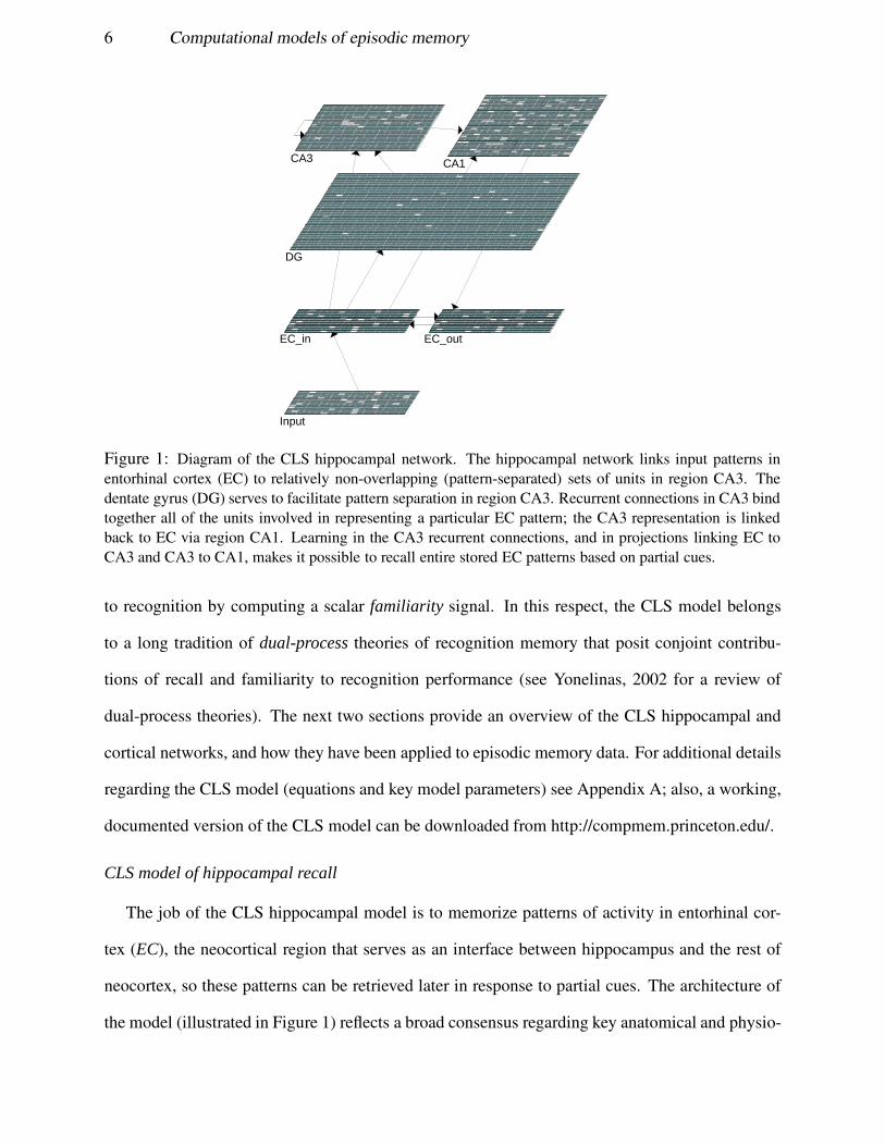
Figure 1: Diagram of the CLS hippocampal network. The hippocampal network links input patterns inentorhinal cortex (EC) to relatively non-overlapping (pattern-separated) sets of units in region CA3. Thedentate gyrus (DG) serves to facilitate pattern separation in region CA3. Recurrent connections in CA3 bindtogether all of the units involved in representing a particular EC pattern; the CA3 representation is linkedback to EC via region CA1. Learning in the CA3 recurrent connections, and in projections linking EC toCA3 and CA3 to CA1, makes it possible to recall entire stored EC patterns based on partial cues.
to recognition by computing a scalar familiarity signal. In this respect, the CLS model belongs
to a long tradition of dual-process theories of recognition memory that posit conjoint contribu-
tions of recall and familiarity to recognition performance (see Yonelinas, 2002 for a review of
dual-process theories). The next two sections provide an overview of the CLS hippocampal and
cortical networks, and how they have been applied to episodic memory data. For additional details
regarding the CLS model (equations and key model parameters) see Appendix A; also, a working,
documented version of the CLS model can be downloaded from http://compmem.princeton.edu/.
CLS model of hippocampal recall
The job of the CLS hippocampal model is to memorize patterns of activity in entorhinal cor-
tex (EC), the neocortical region that serves as an interface between hippocampus and the rest of
neocortex, so these patterns can be retrieved later in response to partial cues. The architecture of
the model (illustrated in Figure 1) reflects a broad consensus regarding key anatomical and physio-
Norman, Detre, & Polyn 7
logical characteristics of different hippocampal subregions (Squire, Shimamura, & Amaral, 1989),
and how these subregions contribute to the overall goal of memorizing cortical patterns. While the
fine-grained details of other hippocampal models may differ slightly from the CLS model, the “big
picture” story (reviewed below) is remarkably consistent across models (Rolls, 1989; Hasselmo &
Wyble, 1997; Meeter, Murre, & Talamini, 2004; Becker, 2005).
In the brain, EC is split into two layers, a superficial layer that primarily sends input into the hip-
pocampus, and a deep layer that primarily receives output from the hippocampus (Witter, Wouter-
lood, Naber, & Van Haeften, 2000); in the model, these layers are referred to as EC in and EC out.
The part of the model corresponding to the hippocampus proper is subdivided into different layers,
corresponding to different anatomical subregions of the hippocampus. At encoding, the hippocam-
pal model binds together sets of co-occurring neocortical features (corresponding to a particular
episode) by linking co-active units in EC in to a cluster of units in region CA3. These CA3 units
serve as the hippocampal representation of the episode. In addition to strengthening feedforward
connections between EC in and CA3, recurrent connections between active CA3 units are also
strengthened. To allow for recall, active CA3 units are linked back to the original pattern of cor-
tical activity via region CA1. Like CA3, region CA1 also contains a representation of the input
pattern. However, unlike the CA3 representation, the CA1 representation is invertible — if an
item’s representation is activated in CA1, well-established connections between CA1 and EC out
allow activity to spread back to the item’s representation in EC out. Thus, CA1 serves to trans-
late between sparse representations in CA3 and more overlapping representations in EC (for more
discussion of this issue, see McClelland & Goddard, 1996 and O’Reilly, Norman, & McClelland,
1998).
The projections described above are updated using the CPCA Hebbian learning rule during the
study phase of the experiment (except for connections between EC and CA1, which are pre-trained
to form an invertible mapping). At test, when a partial version of a stored EC pattern is presented to
the hippocampal model, the model is capable of reactivating the entire CA3 pattern corresponding

8 Computational models of episodic memory
to that item because of learning (in feedforward and recurrent connections) that occurred at study.
Activation then spreads from the item’s CA3 representation back to the item’s EC representation
(via CA1). In this manner, the hippocampal model manages to retrieve a complete version of the
EC pattern in response to a partial cue. This process is typically referred to as pattern completion.
To minimize interference between episodes, the hippocampal model has a built-in bias to assign
relatively non-overlapping (pattern separated) CA3 representations to different episodes. Pattern
separation occurs because of strong feedback inhibition in CA3, which leads to sparse representa-
tions: In the hippocampal model, only the top 4% of units in CA3 (ranked in terms of excitatory
input) are active for any given input pattern. The fact that CA3 units are hard to activate reduces
the odds that a given unit will be active for any two input patterns, thereby leading to pattern
separation.
Pattern separation in CA3 is greatly facilitated by the dentate gyrus (DG). Like CA3, the DG
also receives a projection from EC in. The DG has even sparser representations than CA3, and has
a very strong projection to CA3 (the mossy fiber pathway). In effect, the DG can be viewed as se-
lecting a (nearly) unique representation for each stimulus, and then forcing that representation onto
CA3 via the mossy fiber pathways (see O’Reilly & McClelland, 1994 for a much more detailed
treatment of pattern separation in the hippocampus, and the role of the dentate gyrus in facilitating
pattern separation). Recently, Becker (2005) has argued that neurogenesis in DG plays a key role
in fostering pattern separation: Inserting new neurons and connections into DG ensures that, if two
similar patterns that are fed into DG on different occasions, they will elicit distinct patterns of DG
activity (because the DG connectivity matrix is different on the first vs. second occasion).
To apply the hippocampal model to recognition, Norman and O’Reilly (2003) compared the
test cue (presented on the EC in layer) to the pattern of retrieved information (activated over the
EC out layer). When recalled information matches the test cue, this constitutes evidence that the
item was studied; conversely, mismatch between recalled information and the test cue constitutes

Norman, Detre, & Polyn 9
evidence that the test cue was not studied (e.g., study “rats”; test “rat”; if the hippocampal model
recalls that “rats”-plural was studied, not “rat”-singular, this can serve as grounds for rejection of
“rat”).
Optimizing the dynamics of the hippocampal model As discussed by O’Reilly and McClelland
(1994), the greatest computational challenge faced by the hippocampal model is dealing with the
inherent trade-off between pattern separation and pattern completion. Pattern separation reduces
the extent to which storing a new memory trace damages other, previously stored memory traces.
However, this tendency to assign distinct hippocampal representations to similar EC inputs can
interfere with pattern completion at retrieval: It is very uncommon for retrieval cues to exactly
match stored patterns; if there is a mismatch between the retrieval cue and the to-be-recalled trace,
pattern separation mechanisms might cause the cue to activate a different set of CA3 units than
the original memory trace (so retrieval will not occur). Hasselmo and colleagues (e.g., Hasselmo,
1995; Hasselmo, Wyble, & Wallenstein, 1996; Hasselmo & Wyble, 1997) have also pointed out that
pattern completion can interfere with pattern separation: If, during storage of a new memory, the
hippocampus recalls related memories, such that both old and new memories are simultaneously
active at encoding, these memories will become even more tightly associated (due to Hebbian
learning between co-active neurons) and thus run the risk of blending together.
To counteract these problems, Hasselmo and others have argued that the hippocampus has an
encoding mode, where the functional connectivity of the hippocampus is optimized for storage
of new memories, and a retrieval mode, where the functional connectivity of the hippocampus is
optimized for retrieval of stored memory traces that match the current input.
Two of the most prominent optimizations discussed by Hasselmo are:
• The strength of CA3 recurrents should be larger during retrieval mode than encoding mode.
Increasing the strength of recurrent connections facilitates pattern completion.
• During encoding mode, the primary influence on CA1 activity should be the current input

10 Computational models of episodic memory
pattern in EC. During retrieval mode, the primary influence on CA1 activity should be the
retrieved (“completed”) pattern in CA3.
For discussion of these optimizations as well as others (relating to adjustments in hippocampal
learning rates) see Hasselmo et al. (1996). 1
Hasselmo originally proposed that mode-setting was accomplished by varying the concentration
of the neuromodulatory chemical acetylcholine (ACh). Hasselmo and Wyble (1997) present a
computational model of this process. According to this model, presenting a novel pattern to the
hippocampus activates the basal forebrain, which (in turn) releases ACh into the hippocampus,
triggering encoding mode (see Meeter et al., 2004 for a similar model). For physiological evidence
that ACh triggers the key properties of encoding mode (as listed above), see Hasselmo, Schnell,
and Barkai (1995) and Hasselmo and Schnell (1994).
More recently, Hasselmo and Fehlau (2001) have argued that ACh can not be the only mech-
anism of mode-setting in the hippocampus, because the temporal dynamics of ACh release are
too slow (on the order of seconds) — by the time that ACh is released, the to-be-encoded stim-
ulus may already be gone. Hasselmo and Fehlau (2001) argue that, in order to support more
responsive mode-setting, the ACh-based mechanism discussed above is supplemented by another
mechanism that leverages hippocampal theta oscillations (rhythmic changes in the local field po-
tential, at approximately 4-8 Hz in humans). Specifically, they argue that oscillatory changes in
the concentration of the neurotransmitter GABA cause the hippocampus to flip back and forth
between encoding and retrieval modes several times per second — as such, each stimulus is pro-
cessed (several times) both as a new stimulus to be encoded, and as a “reminder” to retrieve other
stimuli. Hasselmo, Bodelon, and Wyble (2002) present a detailed computational model of this
theta-based mode setting; for physiological evidence in support of this model see Wyble, Linster,
1Yet another optimization, not discussed by Hasselmo, would be to reduce the influence of the dentate gyrus onCA3 at retrieval. As mentioned earlier, the DG’s primary function in the CLS model is to foster pattern separation.Thus, reducing the influence of the DG at retrieval should reduce pattern separation and — through this — boostpattern completion (see Becker, 2005 for additional discussion of this point).

Norman, Detre, & Polyn 11
a) b)Hidden Layer(Perirhinal Cortex)
Input Layer (Lower-Level Cortex)
Figure 2: Illustration of the sharpening of hidden (perirhinal) layer activity patterns in a miniature version ofthe CLS cortical model. (a) shows the network prior to sharpening; perirhinal activity (more active = lightercolor) is relatively undifferentiated. (b) shows the network after CPCA Hebbian learning and inhibitorycompetition produce sharpening; a subset of the units are strongly active, while the remainder are inhibited.
and Hasselmo (2000).
In its current form, the CLS hippocampal model only incorporates a very crude version of mode-
setting (such that EC is the primary influence on CA1 during study of new items, and CA3 is the
primary influence on CA1 during retrieval). Incorporating the other mode-related optimizations
mentioned above (e.g., varying the strength of CA3 recurrents to facilitate encoding vs. retrieval)
should greatly improve the efficacy of the CLS hippocampal model.
CLS model of cortical familiarity
The CLS cortical model consists of an input layer (corresponding to lower regions of the cortical
hierarchy) which projects in a feedforward fashion to a hidden layer (corresponding to perirhinal
cortex). As mentioned earlier, the main function of cortex is to extract statistical regularities in
the environment; the two-layer CLS cortical network (where “perirhinal” hidden units compete to
encode regularities that are present in the input layer) is meant to capture this idea in the simplest
possible fashion.
Because the cortical model uses a small learning rate, it is not capable of pattern completion
following limited exposure to a stimulus. However, it is possible to extract a scalar signal from
the cortical model that reflects stimulus familiarity: In the cortical model, as items are presented
repeatedly, their representations in the upper (perirhinal) layer become sharper: Novel stimuli
weakly activate a large number of perirhinal units, whereas previously presented stimuli strongly
activate a relatively small number of units. Sharpening occurs in the model because Hebbian

12 Computational models of episodic memory
learning specifically tunes some perirhinal units to represent the stimulus. When a stimulus is first
presented, some perirhinal units, by chance, will respond more strongly to the stimulus than other
units. These “winning” units get tuned by CPCA Hebbian learning to respond even more strongly
to the item then next time it is presented; this increased response triggers an increase in feedback
inhibition to units in the layer, resulting in decreased activation of the “losing” units. This latter
property (whereby some initially-responsive units drop out of the stimulus representation as it is
repeated) is broadly consistent with the neurophysiological finding that some perirhinal neurons
show decreased responding as a function of stimulus familiarity (e.g., Xiang & Brown, 1998; Li
et al., 1993); see Section 2.2 (Alternative models of perirhinal familiarity), below, for additional
discussion of single-cell-recording data from perirhinal cortex. Figure 2 illustrates this sharpening
dynamic.2 In the Norman and O’Reilly (2003) paper, cortical familiarity was operationalized
by reading out the activation of the k winning units in the perirhinal layer (where k is a model
parameter that defines the maximum number of units that are allowed to be strongly active at
once), although other methods of operationalizing familiarity are possible.
Because there is more overlap between representations in the cortical model vs. the hippocam-
pal model, the familiarity signal generated by the cortical model has very different operating char-
acteristics than the recall signal generated by the hippocampal model: In contrast to hippocampal
recall, which only occurs when the test cue is very similar to a specific studied item, the corti-
cal familiarity signal tracks — in a graded fashion — the amount of overlap between the test cue
and the full set of studied items. This sensitivity to “global match” is one of the most critical
psychological properties of the familiarity signal (for behavioral evidence that familiarity tracks
global match, see, e.g., Brainerd & Reyna, 1998; Koutstaal, Schacter, & Jackson, 1999; Shiffrin,
Huber, & Marinelli, 1995; Criss & Shiffrin, 2004; see also Section 3 below for discussion of how
abstract models implement a “global match” familiarity process).
2For additional discussion of how competitive learning can lead to sharpening, see, e.g., Grossberg, 1986, Section23, and Grossberg & Stone, 1986, Section 16.
Norman, Detre, & Polyn 13
Importantly, while the Norman and O’Reilly (2003) model focuses on the contribution of
perirhinal cortex in familiarity discrimination, the CLS framework is entirely compatible with
other theories that have emphasized the role of perirhinal cortex in representing high-level con-
junctions of object features (e.g., Bussey, Saksida, & Murray, 2002; Bussey & Saksida, 2002;
Barense, Bussey, Lee, Rogers, Davies, Saksida, Murray, & Graham, 2005). The CLS cortical net-
work performs competitive learning of object features in exactly the manner specified by these
other models; the “sharpening” dynamic described above (which permits familiarity discrimina-
tion) is a byproduct of this feature extraction process. Another important point is that, according
to the CLS model, perirhinal cortex works just like the rest of cortex. Its special role in familiarity
discrimination (and learning of high-level object conjunctions) is attributable to its position at the
top of the cortical hierarchy, which allows it to associate a wider range of features, and also allows
it to respond differentially to novel combinations of these features (when discriminating between
old and new items on a recognition test). For additional discussion of this point, see Norman and
O’Reilly (2003).
Representative prediction from the CLS model
Norman and O’Reilly (2003) showed how, taken together, the hippocampal network and cortical
network can explain a wide range of behavioral findings from recognition and recall list-learning
experiments. Furthermore, because the CLS model maps clearly onto the brain, it is possible to use
the model to address neuroscientific data in addition to (purely) behavioral data. Here, we discuss
a representative model prediction, relating to how target-lure similarity and recognition test format
should interact with hippocampal damage.
The CLS model predicts that cortex and hippocampus can both support good recognition perfor-
mance when lures are not closely related to studied items. However, when lures are closely related
to studied items, hippocampally-based recognition performance should be higher than cortically-
based recognition performance, because of the hippocampus’ ability to assign distinct represen-
14 Computational models of episodic memory
tations to similar stimuli, and its ability to reject lures when they trigger recall that mismatches
the test cue. The model also predicts that effects of target-lure similarity should interact with test
format. Most recognition tests use a yes-no (YN) format where test items are presented one at a
time, and subjects are asked to label them as old or new. The model predicts that cortex should
perform very poorly on YN tests with related lures (because the distributions of familiarity scores
associated with studied items and related lures overlap strongly). However, the model predicts
that cortex should perform much better when given a forced choice between studied items and
corresponding related lures (e.g., “rat” and “rats” are presented simultaneously, and subjects have
to choose which item was studied). In this situation, the model predicts that the mean difference
in familiarity between the studied item and the related lure will be small, but the studied item
should reliably be slightly more familiar than the corresponding related lure (thereby allowing for
correct responding; see Hintzman, 1988 for additional discussion of this idea). Taken together,
these predictions imply that patients with hippocampal damage should perform very poorly on YN
tests with related lures. However, the same patients should show relatively spared performance on
tests with unrelated lures, or when they are given a forced choice between targets and correspond-
ing related lures (since cortex can pick up the slack in both cases). Holdstock, Mayes, Roberts,
Cezayirli, Isaac, O’Reilly, and Norman (2002) and Mayes, Isaac, Downes, Holdstock, Hunkin,
Montaldi, MacDonald, Cezayirli, and Roberts (2001) tested these predictions in a patient with fo-
cal hippocampal damage and obtained the predicted pattern of results; for additional evidence in
support of these predictions, see also Westerberg, Paller, Weintraub, Mesulam, Holdstock, Mayes,
and Reber (2006).
Memory decision-making: A challenge for recognition memory models
There is one major way in which the CLS model is presently underspecified: namely, how to
combine the contributions of hippocampal recall and cortical familiarity when making recognition
decisions. This problem is shared by all dual-process recognition memory models, not just CLS.

Norman, Detre, & Polyn 15
Norman and O’Reilly (2003) treat recognition decision-making as a “black box” that is external
to the network model itself (i.e., the decision process is not itself simulated by a neural network).
This raises two issues: First, at an abstract level, what algorithm should be implemented by the
black box? Second, how could this algorithm be implemented in network form? In their com-
bined cortico-hippocampal simulations, Norman and O’Reilly (2003) used a simple rule where
test items were called “old” if hippocampal recall exceeded a certain value, otherwise, the decision
was made based on familiarity (Jacoby, Yonelinas, & Jennings, 1997). This reflects the common
assumption that recall is more diagnostic than familiarity. However, the diagnosticity of both re-
call and familiarity varies from situation to situation. For example, Norman and O’Reilly (2003)
discuss how recall of unusual features is more diagnostic than recall of common features. Also,
familiarity is less diagnostic when lures are highly similar to studied items, vs. when lures are
less similar to studied items. Ideally, the decision-making algorithm would be able to dynamically
weight the evidence provided by recall of a particular feature (relative to familiarity) based on its
diagnosticity.
However, even if subjects manage to successfully compute the diagnosticity of each pro-
cess, there are many reasons why (in a particular situation) subjects might deviate from this
diagnosticity-based weighting. For example, several studies have found that dual-task demands
hurt recall-based responding more than familiarity-based responding (e.g., Gruppuso, Lindsay, &
Kelley, 1997), suggesting that recall-based responding places stronger demands on cognitive re-
sources than familiarity-based responding. If recall-based responding is generally more demanding
than familiarity-based responding, this could cause subjects to under-attend to recall (even when it
is useful). Furthermore, the reward structure of the task will interact with decision weights (e.g.,
if the task places a high premium on avoiding false alarms, subjects might attend relatively more
to recall; see Malmberg & Xu, in press for additional discussion of how subjects weight recall vs.
familiarity).
Finally, in constructing a model of memory decision-making, it is important to factor in more

16 Computational models of episodic memory
dynamical aspects of the decision-making process. In recent years, models of memory decision-
making have started to shift away from simple signal-detection accounts (where a cutoff is ap-
plied to a static memory strength value), toward models that accumulate evidence across time
(see the chapter by Busemeyer & Johnson in this volume). While these dynamical “evidence-
accumulation” models are more complex than models based on signal-detection theory (in the
sense that they have more parameters), several researchers have demonstrated that evidence-
accumulation models can be implemented using relatively simple neural network architectures
(e.g., Usher & McClelland, 2001). As such, the shift to dynamical decision-making models may
actually make it easier to construct a neural network model of memory decision-making processes.
Overall, incorporating a more accurate model of the decision-making process (in terms of how
recall and familiarity are weighted, in terms of temporal dynamics, and in terms of how this pro-
cess is instantiated in the brain) should greatly increase the predictive utility of extant recognition
memory models.
2.2. Alternative models of perirhinal familiarity
While (as mentioned above) the basic tenets of the CLS hippocampal model are relatively un-
controversial, there is much less agreement about whether the CLS cortical model adequately ac-
counts for perirhinal contributions to recognition memory. Recently, the CLS cortical model was
criticized by Bogacz and Brown (2003), on the grounds that it has inadequate storage capacity.
Bogacz and Brown (2003) showed that, when input patterns are correlated with one another, the
model’s capacity for familiarity discrimination (operationalized as the number of studied stimuli
that the network can distinguish from nonstudied stimuli with 99% accuracy) barely increases as
a function of network size; because of this, the model’s capacity (even in a “brain-sized” network)
falls far short of the documented capacity of human recognition memory (e.g., Standing, 1973).
These capacity problems can be traced back to the CPCA Hebbian learning algorithm used
by Norman and O’Reilly (2003). As discussed by Norman, Newman, and Perotte (2005), CPCA

Norman, Detre, & Polyn 17
Hebbian learning is insufficiently judicious in how it adjusts synaptic strengths: It strengthens
synapses between co-active units even if the target memory is already strong enough to support
recall, and it weakens synapses between active receiving units and all sending units that are in-
active at the end of the trial, even if these units did not actively compete with recall of the target
memory. As a result of this problem, CPCA Hebbian learning ends up over-representing features
that are common to all items in the stimulus set, and under-representing features that are specific
to individual items. Insofar as recognition depends on memory for item-specific features (common
features are, by definition, useless for recognition, because they are shared by both studied items
and lures), this tendency for CPCA Hebbian leaning to under-represent item-specific features re-
sults in poor recognition discrimination. In their paper, Bogacz and Brown (2003) also discuss a
Hebbian familiarity discrimination model developed by Sohal and Hasselmo (2000). This model
operates according to slightly different principles than the CLS cortical model, but it shares the
same basic problem (over-focusing on common features) and thus performs poorly with correlated
input patterns.
Given these capacity concerns, it is worth exploring how well other, recently developed models
of perirhinal familiarity discrimination can address these capacity issues, as well as extant neu-
rophysiological and psychological data on perirhinal contributions to recognition memory. Three
alternative models are discussed below: a model developed by Bogacz and Brown (2003) that uses
anti-Hebbian learning to simulate decreased responding to familiar stimuli; a model developed by
Meeter, Myers, and Gluck (2005) that shows decreased responding to familiar stimuli because of
context-driven adaptation effects; and a model developed by Norman, Newman, Detre, and Polyn
(2006b) that probes the strength of memories by oscillating the amount of feedback inhibition.
The anti-Hebbian model
In contrast to the CLS familiarity model, in which familiarity discrimination was a byproduct
of Hebbian feature extraction, the anti-Hebbian model proposed by Bogacz and Brown posits that

18 Computational models of episodic memory
separate neural populations in perirhinal cortex are involved in representing stimulus features (on
the one hand) vs. familiarity discrimination (on the other). Bogacz and Brown (2003) argue that
neurons involved in familiarity discrimination use an anti-Hebbian learning rule, which weakens
the weights from active pre-synaptic neurons to active post-synaptic neurons, and increases the
weights from inactive pre-synaptic neurons. This anti-Hebbian rule causes neurons that initially
respond to a stimulus to respond less on subsequent presentations of that stimulus.
The primary advantage of the anti-Hebbian model over the CLS model is improved capacity.
Whereas Hebbian learning ends up over-representing common features and under-representing
unique features (resulting in poor overall capacity), anti-Hebbian learning biases the network to
ignore common features and to represent what is distinctive or unusual about individual patterns.
Bogacz and Brown (2003) present a mathematical analysis showing that the anti-Hebbian model’s
capacity for familiarity discrimination (given correlated input patterns) is orders of magnitude
higher than the capacity of a model trained with Hebbian learning.
With regard to neurophysiological data: There are several salient differences in the predictions
made by the anti-Hebbian model vs. the CLS cortical model. A foundational assumption of the Bo-
gacz and Brown (2003) model is that neurons showing steady, above-baseline firing vs. decreased
firing (as a function of stimulus repetition) belong to distinct neural populations: The former group
(showing steady responding) is involved in representing stimulus features, whereas the latter group
is involved in familiarity discrimination. This view implies that it should be impossible to find a
neuron that shows steady responding to some stimuli and decreased responding to other stimuli. In
contrast, the CLS cortical model posits that neurons that show steady (above-baseline) or increased
firing to a given stimulus are the neurons that won the competition to represent this stimulus, and
neurons that show decreased firing are the neurons that lost the competition to represent this stim-
ulus. Furthermore, different neurons will win (vs. lose) the competition for different stimuli. Thus,
contrary to the predictions of the Bogacz and Brown (2003) model, it should be possible to find
a neuron that shows steady (or increased) responding to one stimulus (because it won the com-
Norman, Detre, & Polyn 19
petition to represent that stimulus) and decreased responding to another stimulus (because it lost
the competition to represent that stimulus). More data need to be collected in order to test these
predictions.
The Meeter, Myers, & Gluck (2005) model
The Meeter et al. (2005) model uses the same basic Hebbian learning architecture as Norman
and O’Reilly (2003), with two critical changes: First, they added a neural adaptation mechanism
(such that units become harder to activate after a period of sustained activation). Second, they
are more explicit in considering how context is represented in the input patterns. According to
the Meeter et al. (2005) model, if an item is presented in a particular context (e.g., in a particular
room, on a particular computer screen, in a particular font), then the units activated by the item
become linked to the units activated by contextual features. As a result of this item-context linkage,
whenever the subject is in that context (and, consequently, context-sensitive neurons are firing),
the linked item units will receive a small amount of activation. Over time, this low-level input
from contextual features will lead to adaptation in the linked item units, thereby making them less
likely to fire to subsequent repetitions of that item. In the Meeter et al. (2005) model, “context”
is operationalized as a set of input units that receive constant (above-zero) excitation throughout
the experiment; apart from this fact, context features function identically to units that represent the
features of individual items.
This model has several attractive properties with regard to explaining data on single-unit activity
in perirhinal cortex. It can account for the basic decrease in the neural response triggered by
familiar vs. novel stimuli. Moreover, it provides an elegant explanation of why some perirhinal
neurons do not show decreased responding with stimulus repetition. Contrary to the Bogacz and
Brown (2003) idea that neurons showing decreased vs. steady responding come from separate
populations (with distinct learning rules), the Meeter et al. (2005) model explains this difference
in terms of a simple difference in context-sensitivity. Specifically: According to the Meeter et al.

20 Computational models of episodic memory
(2005) model, neurons that receive input from a large number of contextual features will show
decreased responding to repeated stimuli (insofar as these contextual inputs will cause the neuron
to be tonically active, leading to adaptation), whereas neurons that are relatively insensitive to
contextual features will not show decreased responding.
The most salient prediction of the Meeter model is that familiarity should be highly context-
sensitive: Insofar as the strengthened context-item association formed at study is what causes
adaptation, changing context between study and test should eliminate adaptation and thus eliminate
the decrement in responding to previously studied stimuli. This prediction has not yet been tested.
With regard to capacity, the Meeter et al. (2005) model uses the same Hebbian learning mechanism
as the CLS model, so the same capacity issues that were raised by Bogacz and Brown (2003) (with
regard to the CLS model) also apply here.
The oscillating learning algorithm (Norman et al., in press)
In response to the aforementioned problems with CPCA Hebbian learning, Norman et al. (in
press; see also Norman et al., 2005) developed a new learning algorithm that (like CPCA Hebbian
learning) does feature extraction, but (unlike CPCA Hebbian learning) is more judicious in how
it adjusts synapses: It selectively strengthens weak parts of target memories (vs. parts that are
already strong), and selectively punishes strong competitors. The algorithm memorizes patterns in
the following manner:
• First, the to-be-learned (target) pattern is imposed on the network (via external inputs).
• Second, the algorithm identifies weak parts of the target memory by raising feedback inhibi-
tion above baseline. This increase can be viewed as a “stress test” on the target memory. If a
target unit is receiving relatively little collateral support from other target units, such that its
net input is just above threshold, raising inhibition will trigger a decrease in the activation of
that unit. The algorithm then acts to strengthen units that drop out, by increasing connections
coming into these units units from active senders.
Norman, Detre, & Polyn 21
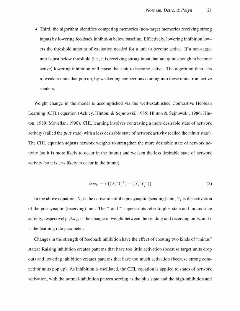
• Third, the algorithm identifies competing memories (non-target memories receiving strong
input) by lowering feedback inhibition below baseline. Effectively, lowering inhibition low-
ers the threshold amount of excitation needed for a unit to become active. If a non-target
unit is just below threshold (i.e., it is receiving strong input, but not quite enough to become
active) lowering inhibition will cause that unit to become active. The algorithm then acts
to weaken units that pop up, by weakening connections coming into these units from active
senders.
Weight change in the model is accomplished via the well-established Contrastive Hebbian
Learning (CHL) equation (Ackley, Hinton, & Sejnowski, 1985; Hinton & Sejnowski, 1986; Hin-
ton, 1989; Movellan, 1990). CHL learning involves contrasting a more desirable state of network
activity (called the plus state) with a less desirable state of network activity (called the minus state).
The CHL equation adjusts network weights to strengthen the more desirable state of network ac-
tivity (so it is more likely to occur in the future) and weaken the less desirable state of network
activity (so it is less likely to occur in the future).
∆wij = ε(
(X+i Y +
j ) − (X−
i Y −
j ))
(2)
In the above equation, Xi is the activation of the presynaptic (sending) unit, Yj is the activation
of the postsynaptic (receiving) unit. The + and − superscripts refer to plus-state and minus-state
activity, respectively. ∆wij is the change in weight between the sending and receiving units, and ε
is the learning rate parameter.
Changes in the strength of feedback inhibition have the effect of creating two kinds of “minus”
states: Raising inhibition creates patterns that have too little activation (because target units drop
out) and lowering inhibition creates patterns that have too much activation (because strong com-
petitor units pop up). As inhibition is oscillated, the CHL equation is applied to states of network
activation, with the normal-inhibition pattern serving as the plus state and the high-inhibition and
22 Computational models of episodic memory
low-inhibition patterns serving as minus states (Norman et al., 2006b).
Because strengthening is limited to weak target features, the oscillating algorithm avoids the
problem of “over-strengthening of common features” that plagues Hebbian learning. Also, the
oscillating algorithm’s ability to selectively punish competitors helps to prevent similar mem-
ories from collapsing into one another: Whenever memories start to blend together, they also
start to compete with one another at retrieval, and the competitor-punishment mechanism pushes
them apart.3 Norman et al. (2006b) discuss how the oscillating algorithm may be implemented in
the brain by neural theta oscillations (insofar as these oscillations involve regular changes in the
strength of neural inhibition, and are present in both cortex and the hippocampus).
Recently, Norman et al. (2005) explored the oscillating algorithm’s ability to do familiarity dis-
crimination. These simulations used a simple two-layer network: Patterns were presented to the
lower part of the network (the input/output layer). The upper part of the network (the hidden layer)
was allowed to self-organize according to the dictates of the learning algorithm. Every unit in the
input/output layer was connected to every input/output unit (including itself) and to every hidden
unit via modifiable, symmetric weights. A familiarity signal can be extracted from this network
by looking at how activation changes when inhibition is raised above its baseline value: Weak (un-
familiar) memories show a larger decrease in activation than strong (familiar) memories. Norman
et al. (2005) tested the network’s ability to discriminate between 100 studied and 100 nonstudied
patterns, where the average pairwise overlap between any two patterns (studied or nonstudied) was
41%. After 10 study presentations, discrimination accuracy was effectively at ceiling (99%). In
this same situation, the performance of the Norman and O’Reilly (2003) CLS familiarity model
(trained with CPCA Hebbian learning) was close to chance. This finding shows that the oscil-
lating algorithm can show good familiarity discrimination in exactly the kind of situation (i.e.,
3Importantly, unlike the CLS hippocampal model described earlier (which automatically enacts pattern separation,regardless of similarity), the oscillating algorithm is only concerned that memories observe a minimum separationfrom one another. So long as this constraint is met, memories in the cortical network simulated here are free to overlapaccording to their similarity (thereby allowing the network to enact similarity-based generalization).

Norman, Detre, & Polyn 23
high correlation between patterns) where the CLS familiarity model performs poorly. Although
Norman et al. (2005) have not yet carried out the requisite mathematical analyses, it is quite pos-
sible that the oscillating algorithm’s capacity for supporting familiarity-based discrimination, in
a brain-sized network, will be large enough to account for the vast capacity of human familiarity
discrimination.
3. Abstract models of recognition and recall
In addition to the biologically-based models discussed above, there is a rich tradition of re-
searchers building more abstract computational models of episodic memory. Although there is
considerable diversity within the realm of abstract memory models, most of the abstract models
that are currently being developed share a common set of properties: At study, memory traces are
placed separately in a long-term store; because of this “separate storage” postulate, acquiring new
memory traces does not affect the integrity of previously stored memory traces. At test, the model
computes the match between the test cue and all of the items stored in memory. This item-by-item
match information can be summed across all items to compute a “global match” familiarity signal.
Some abstract models that conform to this overall structure are SAM (Raaijmakers & Shiffrin,
1981; Gillund & Shiffrin, 1984; Mensink & Raaijmakers, 1988), REM (Shiffrin & Steyvers, 1997;
Malmberg, Holden, & Shiffrin, 2004a), MINERVA 2 (Hintzman, 1988), and NEMO (Kahana &
Sekuler, 2002). Some notable exceptions to this general rule include the TODAM model (Mur-
dock, 1993) and the Matrix model (Humphreys, Bain, & Pike, 1989), which store memory traces
in a composite fashion (instead of storing them separately).
One of the most important properties of global matching models is that the match computation
weights multiple matches to a single trace more highly than the same total number of matches,
spread out across multiple memory traces (e.g., a test cue that matches two features of one item
yields a higher familiarity signal than a test cue that matches one feature of each of two items);
24 Computational models of episodic memory
see Clark and Gronlund (1996) for additional discussion of this point. Among other things, this
property gives global matching models the ability to perform associative recognition (i.e., to dis-
criminate pairs of stimuli that were studied together vs. stimuli that were studied separately).
Different models achieve this sensitivity to conjunctions in different ways. For example, in
MINERVA 2, memory traces are vectors where each element is 1 (indicating that a feature is
present), -1 (indicating that the feature is absent), and 0 (indicating that the feature is unknown).
To compute global match, MINERVA 2 first computes the match between the test cue and each
trace i stored in memory. Match is operationalized as the cue-trace dot product, divided by the
number of features contributing to the dot product:
Si =
N∑
j=1
PjTi,j
Ni
(3)
Si is the match value, Pj is the value of feature j in the cue, Ti,j is the value of feature j in trace
i, N is the number of features, and Ni is the number of features where either the cue or trace is
nonzero.
Next, MINERVA 2 cubes each of these individual match scores to compute an “activation”
value Ai for each trace.
Ai = S3i (4)
Finally, these activation values are summed together across the M traces in memory to yield an
“echo intensity” (global match) score I:
I =M
∑
i=1
Ai (5)
MINERVA 2 shows sensitivity to conjunctions because matches spread across multiple stored
Norman, Detre, & Polyn 25
traces are combined in an additive fashion, but (because of the cube rule) multiple matches to a
single trace are combined in a positively accelerated fashion. For example, consider the difference
between two traces with match values Si of .5, vs. one trace with a match value Si of 1.0. Because
of the cube rule, the total match value I in the former case is .53 + .53 = .25 whereas in the latter
case I = 1.03 = 1.0.
The NEMO model (Kahana & Sekuler, 2002) achieves sensitivity to conjunctions in a similar
fashion: First, NEMO computes a vector distance d(i, j) between the cue and the memory trace
(note: small distance = high similarity). Next, the distance value is passed through an exponential
function, which — like the cube function — has the effect of emphasizing close matches (i.e.,
small distances) relative to weaker matches (i.e., large distances):
η(i, j) = e−τd(i,j) (6)
In the above equation, η(i, j) is the adjusted similarity score, and τ is a model parameter that
determines the steepness of the generalization curve (i.e., how close does a match have to be in
order to contribute strongly to the overall “summed similarity” score).
In abstract models, the same “match” rule that is used to compute the global-match familiarity
signal is also used when simulating recall, although the specific way in which the match rule is
used during recall differs from model to model. For example, MINERVA 2 simulates recall by
computing a weighted sum C of all of the items i stored in memory, where each item is weighted
by its match to the test cue. The jth element of C is given by:
Cj =
M∑
i=1
AiTi,j (7)
In contrast, models like SAM and REM use the individual match scores to determine which
(single) memory trace will be “sampled” for recall (see Section 3.1 below).
26 Computational models of episodic memory
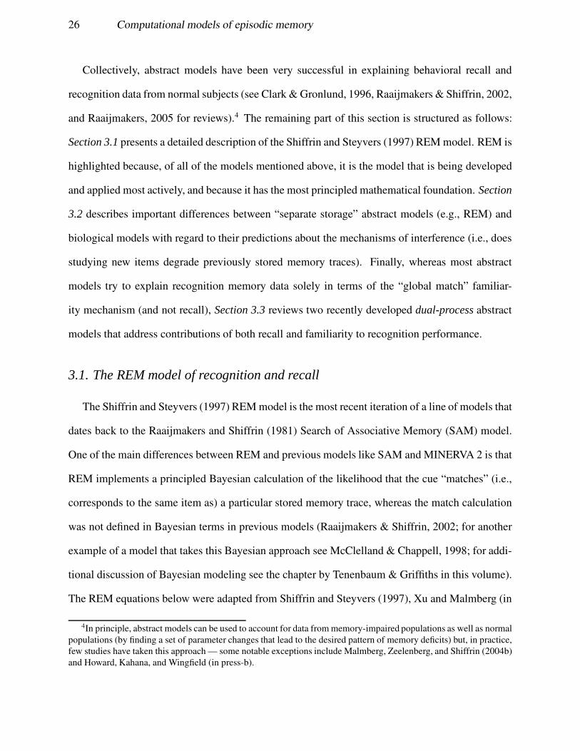
Collectively, abstract models have been very successful in explaining behavioral recall and
recognition data from normal subjects (see Clark & Gronlund, 1996, Raaijmakers & Shiffrin, 2002,
and Raaijmakers, 2005 for reviews).4 The remaining part of this section is structured as follows:
Section 3.1 presents a detailed description of the Shiffrin and Steyvers (1997) REM model. REM is
highlighted because, of all of the models mentioned above, it is the model that is being developed
and applied most actively, and because it has the most principled mathematical foundation. Section
3.2 describes important differences between “separate storage” abstract models (e.g., REM) and
biological models with regard to their predictions about the mechanisms of interference (i.e., does
studying new items degrade previously stored memory traces). Finally, whereas most abstract
models try to explain recognition memory data solely in terms of the “global match” familiar-
ity mechanism (and not recall), Section 3.3 reviews two recently developed dual-process abstract
models that address contributions of both recall and familiarity to recognition performance.
3.1. The REM model of recognition and recall
The Shiffrin and Steyvers (1997) REM model is the most recent iteration of a line of models that
dates back to the Raaijmakers and Shiffrin (1981) Search of Associative Memory (SAM) model.
One of the main differences between REM and previous models like SAM and MINERVA 2 is that
REM implements a principled Bayesian calculation of the likelihood that the cue “matches” (i.e.,
corresponds to the same item as) a particular stored memory trace, whereas the match calculation
was not defined in Bayesian terms in previous models (Raaijmakers & Shiffrin, 2002; for another
example of a model that takes this Bayesian approach see McClelland & Chappell, 1998; for addi-
tional discussion of Bayesian modeling see the chapter by Tenenbaum & Griffiths in this volume).
The REM equations below were adapted from Shiffrin and Steyvers (1997), Xu and Malmberg (in
4In principle, abstract models can be used to account for data from memory-impaired populations as well as normalpopulations (by finding a set of parameter changes that lead to the desired pattern of memory deficits) but, in practice,few studies have taken this approach — some notable exceptions include Malmberg, Zeelenberg, and Shiffrin (2004b)and Howard, Kahana, and Wingfield (in press-b).
Norman, Detre, & Polyn 27
press) and Malmberg and Shiffrin (2005).
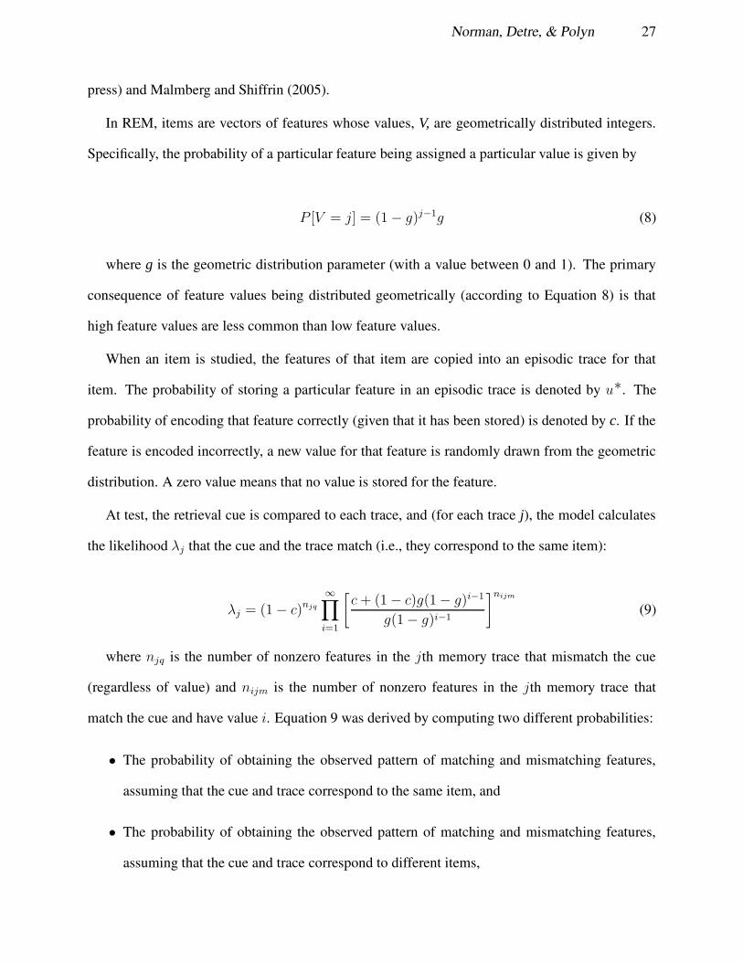
In REM, items are vectors of features whose values, V, are geometrically distributed integers.
Specifically, the probability of a particular feature being assigned a particular value is given by
P [V = j] = (1 − g)j−1g (8)
where g is the geometric distribution parameter (with a value between 0 and 1). The primary
consequence of feature values being distributed geometrically (according to Equation 8) is that
high feature values are less common than low feature values.
When an item is studied, the features of that item are copied into an episodic trace for that
item. The probability of storing a particular feature in an episodic trace is denoted by u∗. The
probability of encoding that feature correctly (given that it has been stored) is denoted by c. If the
feature is encoded incorrectly, a new value for that feature is randomly drawn from the geometric
distribution. A zero value means that no value is stored for the feature.
At test, the retrieval cue is compared to each trace, and (for each trace j), the model calculates
the likelihood λj that the cue and the trace match (i.e., they correspond to the same item):
λj = (1 − c)njq
∞∏
i=1
[
c + (1 − c)g(1 − g)i−1
g(1 − g)i−1
]nijm
(9)
where njq is the number of nonzero features in the jth memory trace that mismatch the cue
(regardless of value) and nijm is the number of nonzero features in the jth memory trace that
match the cue and have value i. Equation 9 was derived by computing two different probabilities:
• The probability of obtaining the observed pattern of matching and mismatching features,
assuming that the cue and trace correspond to the same item, and
• The probability of obtaining the observed pattern of matching and mismatching features,
assuming that the cue and trace correspond to different items,
28 Computational models of episodic memory
The likelihood value λj is computed by dividing the former probability by the latter. Shiffrin
and Steyvers (1997), Appendix A, contains a detailed derivation of Equation 9.
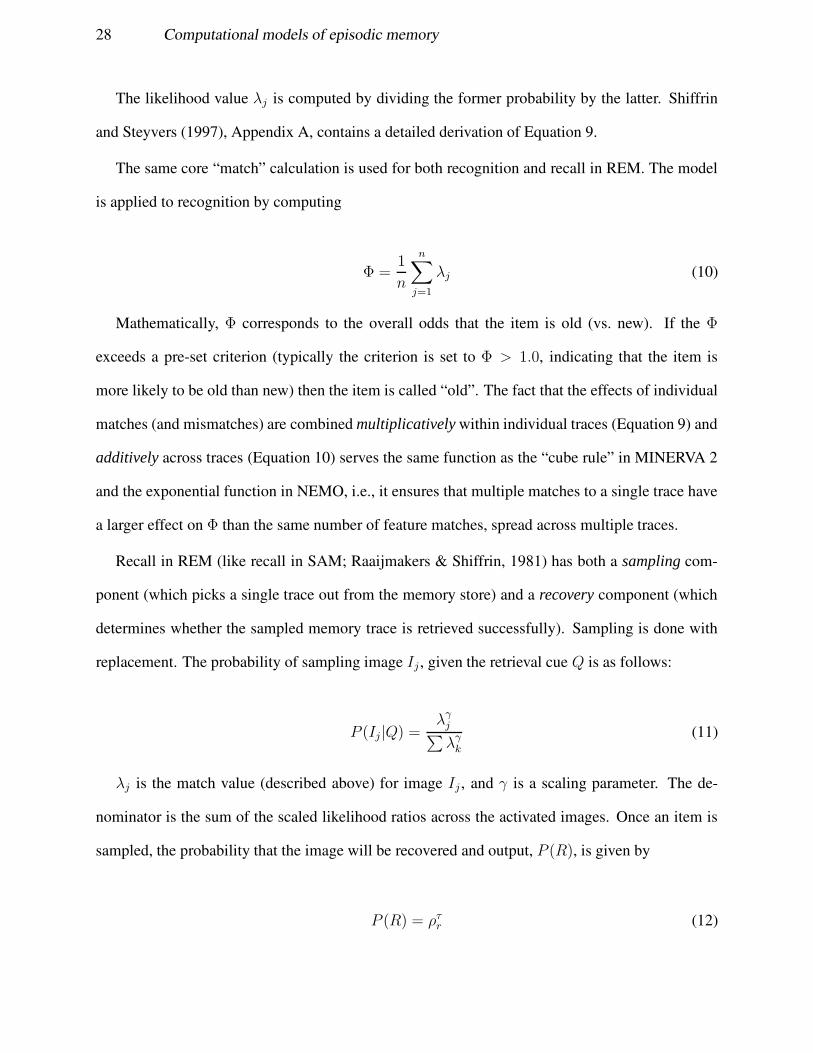
The same core “match” calculation is used for both recognition and recall in REM. The model
is applied to recognition by computing
Φ =1
n
n∑
j=1
λj (10)
Mathematically, Φ corresponds to the overall odds that the item is old (vs. new). If the Φ
exceeds a pre-set criterion (typically the criterion is set to Φ > 1.0, indicating that the item is
more likely to be old than new) then the item is called “old”. The fact that the effects of individual
matches (and mismatches) are combined multiplicatively within individual traces (Equation 9) and
additively across traces (Equation 10) serves the same function as the “cube rule” in MINERVA 2
and the exponential function in NEMO, i.e., it ensures that multiple matches to a single trace have
a larger effect on Φ than the same number of feature matches, spread across multiple traces.
Recall in REM (like recall in SAM; Raaijmakers & Shiffrin, 1981) has both a sampling com-
ponent (which picks a single trace out from the memory store) and a recovery component (which
determines whether the sampled memory trace is retrieved successfully). Sampling is done with
replacement. The probability of sampling image Ij , given the retrieval cue Q is as follows:
P (Ij|Q) =λ
γj
∑
λγk
(11)
λj is the match value (described above) for image Ij , and γ is a scaling parameter. The de-
nominator is the sum of the scaled likelihood ratios across the activated images. Once an item is
sampled, the probability that the image will be recovered and output, P (R), is given by
P (R) = ρτr (12)

Norman, Detre, & Polyn 29
where ρr is the proportion of correctly stored item features in that image and τ is a scaling
parameter. Thus, in REM, well-encoded items are more likely to be recovered than poorly-encoded
items.
Representative REM results
Researchers have demonstrated that REM can explain a wide range of episodic memory find-
ings. For example, Shiffrin and Steyvers (1997) demonstrated that the “global match” familiarity
mechanism described above can account for the word frequency mirror effect: the finding that
subjects make more false alarms to high-frequency lures vs. low-frequency lures, and that sub-
jects make more correct “old” responses to low-frequency targets vs. high-frequency targets (e.g.,
Glanzer, Adams, Iverson, & Kim, 1993). REM’s account of word frequency effects is based on the
idea that low-frequency (LF) words have more unusual features than high-frequency (HF) words;
specifically, REM can fit the observed pattern of word frequency effects by using a slightly lower
value of the geometric distribution parameter g when generating LF items, which results in these
items having slightly higher (and thus more unusual) feature values (see Equation 8). The fact that
LF items have unusual features has two implications: First, it means that LF lures are not likely
to spuriously match stored memory traces — this explains why there are fewer LF false alarms
than HF false alarms. Second, it means that, when LF cues do match stored traces, this is strong
evidence that the item was studied (because matches to unusual features are unlikely to occur due
to chance); as such, LF targets tend to trigger high likelihood (λ) values, which explains why the
hit rate is higher for LF targets than HF targets.
One implication of this account is that, if one could engineer a situation where the (unusual)
features of LF lures match stored memory traces as often as the (more common) features of HF
lures, subjects will show a higher false alarm rate for LF lures than HF lures (the reverse of the nor-
mal pattern). This prediction was tested and confirmed by Malmberg et al. (2004a), who induced
a high rate of “spurious match” for low-frequency lures by using lures that were highly similar to

30 Computational models of episodic memory
studied items (e.g., study “yachts”, test with “yacht”).
3.2. Differences in how models explain interference
One important difference between “separate storage” abstract models like REM and biological
models like CLS relates to sources of interference. In REM, memory traces are stored in a non-
interfering fashion, and interference arises at test (whenever the test cue matches memory traces
other than the target memory trace).5 For example, SAM and REM predict that strengthening
some list items (by presenting them repeatedly) will impair recall of non-strengthened items, by
increasing the odds that the strengthened items will be sampled instead of non-strengthened items
(Malmberg & Shiffrin, 2005). Effectively, the model’s ability to sample these non-strengthened
items is blocked by sampling of the strengthened items.
Biological models, like abstract models, posit that interference can occur at test (due to com-
petition between the target memory and non-target memories). However, in contrast to models
like REM, biological models also posit that interference can occur at study: Insofar as learning in
biological models involves both strengthening and weakening of synapses, adjusting synapses to
store one memory could end up weakening other memories that also rely on those synapses. This
trace weakening process is sometimes referred to as structural interference (Murnane & Shiffrin,
1991) or unlearning (e.g., Melton & Irwin, 1940).
Models like SAM and REM have focused on interference at test, as opposed to structural inter-
ference at study, for two reasons:
• The first reason is parsimony: Models that rely entirely on interference at test can account for
a very wide range of forgetting data. In particular, Mensink and Raaijmakers (1988) showed
that a variant of the SAM model can account for several phenomena that were previously
5Within the realm of abstract models positing interference-at-test, there is some controversy about whether inter-ference arises from spurious matches to other items on the study list, as opposed to spurious matches to memory tracesfrom outside the experimental context; see Dennis and Humphreys (2001) and Criss and Shiffrin (2004) for contrastingperspectives on this issue.

Norman, Detre, & Polyn 31
attributed to unlearning (e.g., retroactive interference in AB-AC interference paradigms;
Barnes & Underwood, 1959).
• The second reason is that it is unclear how to instantiate structural interference properly
within a separate-storage framework. For example, in REM, structural interference would
presumably involve deletion of features from episodic traces, but it is unclear which features
to delete. Biologically-based neural network models fare better in this regard, insofar as
these models incorporate synaptic learning rules that explicitly specify how to adjust synaptic
strengths (upward or downward) as a function of presynaptic and postsynaptic activity.
The most important open issue, with regard to modeling interference and forgetting, is whether
there are any results in the literature that can only be explained by positing trace-weakening mech-
anisms. Michael Anderson has argued that certain findings in the retrieval-induced forgetting lit-
erature may meet this criterion (see Anderson, 2003 for a review). In retrieval-induced forgetting
experiments, subjects study a list of items, and then a subset of the studied items are strengthened
during a second “practice” phase. Anderson and others have found that manipulations that affect
the degree of retrieval competition during the practice phase (e.g., whether subjects are given a
well-specified cue or a poorly-specified cue; Anderson, Bjork, & Bjork, 2000) can affect the ex-
tent to which non-practiced items are forgotten, without affecting the extent to which practiced
items are strengthened. Anderson (2003) explains these results in terms of the idea that (i) com-
petitors are weakened during memory retrieval, and (ii) the degree of weakening is proportional
to the degree of competition.6 Anderson also points out that simple “blocking” accounts of for-
getting may have difficulty explaining the observed pattern of results (increased forgetting without
increased strengthening): According to these blocking accounts, forgetting of non-strengthened
items is a direct consequence of strengthened items being recalled in place of non-strengthened
6See Norman, Newman, & Detre, 2006a for a neural network model of retrieval-induced forgetting that instanti-ates these ideas about competitor-weakening; the model uses the oscillating learning algorithm described earlier tostrengthen the practiced item and weaken competitors.
32 Computational models of episodic memory
items; as such, practice manipulations that lead to the same amount of strengthening should lead
to the same amount of forgetting. At this point, it is unclear whether separate-storage models like
REM (which are considerably more sophisticated than the simple blocking theories described by
Anderson, 2003) can account for the retrieval-induced forgetting results described here.
3.3. Abstract models and dual-process theories
Abstract models have traditionally taken a single-process approach to recognition, whereby
they try to explain recognition performance exclusively in terms of the global match familiarity
process (without positing that recall of specific details contributes to recognition). As with the
structural-interference issue above, the main reason that abstract models have taken this approach
is parsimony: The single-process approach has been extremely successful in accounting for recog-
nition data, hence there is no need to complicate the model by positing that recall contributes
routinely to recognition judgments. However, more recently, Malmberg et al. (2004a) and Xu and
Malmberg (in press) have identified some data patterns (from paradigms that use lures that are
closely related to studied items) that can not be fully explained using the REM familiarity process.
Specifically, studies using related lures (e.g., switched-plurality lures: study “rats”, test “rat”) have
found that increasing the number of study presentations of “rats” increases hits, but does not re-
liably increase false recognition of similar lures like “rat”. Dual-process models can explain this
result in terms of the idea that increased study of “rats” increases the familiarity of “rat” (which
tends to boost false recognition), but it also increases the odds that subjects will recall that they
studied “rats”, not “rat” (Hintzman, Curran, & Oppy, 1992). Malmberg et al. (2004a) showed that
the REM global match process can not simultaneously generate an increase in hit rates, coupled
with no change (or a decrease) in false alarm rates to similar lures (see Xu & Malmberg, in press
for a similar finding, using an associative recognition paradigm).
In response to this issue, Malmberg et al. (2004a) developed a dual-process REM model of
recognition, which incorporates both the REM “global match” familiarity judgment and the REM

Norman, Detre, & Polyn 33
recall process described earlier. This model operates in the following manner: First, stimulus
familiarity is computed (using Equation 9). If familiarity is below a threshold value, the item is
called “new”. If familiarity is above the threshold value, the recall process is engaged. The model
samples a single memory trace and attempts to recover the contents of that trace. If recovery
succeeds and the recovered item matches the test cue, the item is called “old”. If recovery succeeds
and the recovered item mismatches the test cue (e.g., the model recalls “rats” but the test cue
is “rat”), the item is called “new”. If the recovery process fails, the model guesses “old” with
probability γ.7 The addition of this extra recall process allows the model to accommodate the
combination of increasing hits and no increase in false alarms to similar lures.
The SAC model Reder’s SAC (Source of Activation Confusion) model (e.g., Reder, Nhouy-
vanisvong, Schunn, Ayers, Angstadt, & Hiraki, 2000) takes a different approach to simulating
contributions of recall and familiarity to recognition memory. In the SAC model, items are rep-
resented as nodes in a network; episodic memory traces are represented as special nodes that are
linked both to the item and to a node representing the experimental context. Activation is allowed
to spread at test; the degree of spreading activation coming out of a node is a function of the node’s
activation and also the number of connections coming out of the node (the more connections, the
less activation that spreads per connection; for discussion of empirical evidence that supports this
“fan effect” assumption, see Anderson & Reder, 1999; see also Anderson & Lebiere, 1998 for dis-
cussion of another model that incorporates this assumption). In SAC, familiarity is a function of
the activation of the item node itself, whereas recall is a function of the activation of the episodic
node that was created when the item was studied.
Reder et al. (2000) demonstrated that the SAC model can account for word frequency mirror
effects. According to SAC, the false alarm portion of the mirror effect (false alarms to HF lures >
7To accommodate the idea that subjects rely more on recall in some situations than others (see the Memory decision-making section above), the dual-process version of REM includes an extra model parameter (a) that scales the proba-bility of using recall on a given trial.

34 Computational models of episodic memory
false alarms to LF lures) is due to familiarity, and the hit-rate portion of the mirror effect (hit rate
for LF targets > hit rate for HF targets) is due to recall (for similar views, see Joordens & Hockley,
2000; Hirshman, Fisher, Henthorn, Arndt, & Passannante, 2002). In SAC, the fact that HF lures
have been presented more often than LF lures (prior to the experiment) gives them a higher baseline
level of activation, and — through this — a higher level of familiarity. The fact that LF targets are
linked to fewer pre-experimental contexts than HF targets, and thus have a smaller “fan factor”,
means that activity can spread more efficiently to the “episodic node” associated with the study
event (leading to a higher hit rate for LF items).
Reder et al. (2000) argue that this dual-process account of mirror effects is preferable to the
REM account insofar as it models frequency differences in terms of actual differences in the num-
ber of pre-experimental presentations, instead of the idea (used by REM) that LF words have more
unusual features than HF words. However, it remains to be seen whether the Reder et al. (2000)
model provides a better overall account of word frequency effects than REM (in terms of model
fit, and in terms of novel, validated predictions).
4. Context, free recall and active maintenance
Up to this point, this chapter has discussed accounts of how the memory system responds to
a particular cue, but it has not yet touched on how the memory system behaves when external
cues are less well-specified, and subjects have to generate their own cues in order to target a
particular memory (or set of memories). Take the scenario of trying to remember where you left
your keys. The most common advice in this situation is to reinstate your mental context as a means
of prompting recall — if you succeed in remembering what you were doing and what you were
thinking earlier in the day, this will boost the probability of recalling where you left the keys. This
idea of reinstating mental context plays a key role in theories of strategic memory search. Multiple
laboratory paradigms have been developed to examine this process of strategic memory search.

Norman, Detre, & Polyn 35
The most commonly used paradigm is free recall, where subjects are given a word list and are then
asked to retrieve the studied word list in any order. Section 4.1 describes an abstract modeling
framework, the Temporal Context Model (TCM; Howard & Kahana, 2002), that has proved to
be very useful in understanding how we selectively retrieve memories from a particular temporal
context in free recall experiments. Section 4.2 discusses methods for implementing TCM dynamics
in biologically-based neural network models.
4.1. The temporal context model (TCM)
TCM is the most recent in a long succession of models that use a drifting mental context to
explain memory targeting (e.g., Mensink & Raaijmakers, 1988; Estes, 1955). The basic idea behind
these models is that the subject’s inner mental context (comprised of the constellation of thoughts
that are active at a particular moment) changes gradually over time. Mensink and Raaijmakers
(1988) instantiate this idea in terms of a binary context vector, where each element of this context
vector is updated (with some probability) on each time step; the higher the probability of updating,
the faster the context vector drifts over time. During the study phase of a memory experiment,
items are associated with the state of the context vector (at the time of presentation). At test, the
recall process is initiated by cuing with the current state of the context vector, which (in turn)
triggers retrieval of items that were associated with these contextual elements at study.
The main difference between TCM and previous contextual-drift models like Mensink and
Raaijmakers (1988) is that — in TCM — context does not drift randomly. Rather, contextual
updating is driven by the features of the items being studied. More precisely, the state of the
context vector at time i, ti, is given by:
ti = ρiti−1 + βtINi , (13)
where β is a free parameter that determines the rate of contextual drift, ρi is chosen at each
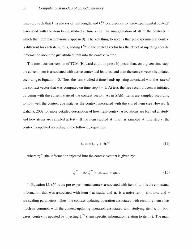
36 Computational models of episodic memory
time step such that ti is always of unit length, and tINi corresponds to “pre-experimental context”
associated with the item being studied at time i (i.e., an amalgamation of all of the contexts in
which that item has previously appeared). The key thing to note is that pre-experimental context
is different for each item; thus, adding tINi to the context vector has the effect of injecting specific
information about the just-studied item into the context vector.
The most current version of TCM (Howard et al., in press-b) posits that, on a given time step,
the current item is associated with active contextual features, and then the context vector is updated
according to Equation 13. Thus, the item studied at time i ends up being associated with the state of
the context vector that was computed on time step i − 1. At test, the free recall process is initiated
by cuing with the current state of the context vector. As in SAM, items are sampled according
to how well the context cue matches the context associated with the stored item (see Howard &
Kahana, 2002 for more detailed description of how item-context associations are formed at study,
and how items are sampled at test). If the item studied at time i is sampled at time step r, the
context is updated according to the following equations:
tr = ρitr−1 + βtINr , (14)
where tINr (the information injected into the context vector) is given by:
tINr = αOt
INi + αNti−1 + ηnr. (15)
In Equation 15, tINi is the pre-experimental context associated with item i, ti−1 is the contextual
information that was associated with item i at study, and nr is a noise term. αO, αN , and η
are scaling parameters. Thus, the context-updating operation associated with recalling item i has
much in common with the context-updating operation associated with studying item i. In both
cases, context is updated by injecting tINi (item-specific information relating to item i). The main

Norman, Detre, & Polyn 37
difference, apart from the noise term, is that context is also updated with ti−1, the state of the
context vector at the time the (just-retrieved) item was studied. This latter updating operation can
be construed as “mentally jumping back in time” to the moment when the (just-retrieved) item was
studied. As discussed below, the two kinds of updating mentioned here (tINi vs. ti−1) have distinct
effects on recall transition probabilities. Once the context vector is updated, it is used to cue for
additional items, which leads to additional updating of the context vector, and so on.
How TCM accounts for recall data
Contextual drift models (in general) and TCM (in particular) can account for a wide range of
free recall findings; some representative findings are discussed in this section.
As one example, contextual drift models provide an elegant account of the long-term recency
effect in free recall. Circa 1970, it was believed that recency effects (better recall of items from the
end of the list) were attributable to the fact that recently presented items were still being held in a
short-term memory buffer. As such, manipulations that disrupt this buffer (e.g., a distraction-filled
retention interval) should sharply reduce recency effects. However, Bjork and Whitten (1974) and
other studies have since demonstrated that recency effects can still be observed after a distraction-
filled delay. Bjork and Whitten (1974) showed that the key determinant of recency is the ratio of
the time elapsed since study of item A vs. and the time elapsed since study of item B; the smaller
this ratio is (indicating that A was presented relatively more recently than B), the better A will
be recalled relative to B (Glenberg, Bradley, Stevenson, Kraus, Tkachuk, Gretz, Fish, & Turpin,
1980). This can be explained by contextual drift models, in the following manner:
• Because of contextual drift, the current test context (being used as a cue) matches the context
associated with recently presented items more than the context associated with less recently
presented items.
• Since recall is a competitive process, recall of a particular trace is a function of the match
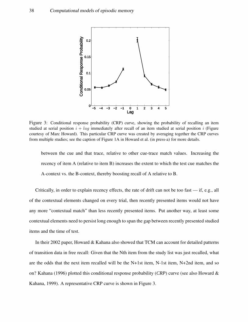
38 Computational models of episodic memory
−5 −4 −3 −2 −1 0 1 2 3 4 50
0.05
0.1
0.15
0.2
Lag
Con
ditio
nal R
espo
nse
Pro
babi
lity
−5 −4 −3 −2 −1 0 1 2 3 4 50
0.05
0.1
0.15
0.2
Lag
Con
ditio
nal R
espo
nse
Pro
babi
lity
−5 −4 −3 −2 −1 0 1 2 3 4 50
0.05
0.1
0.15
0.2
Lag
Con
ditio
nal R
espo
nse
Pro
babi
lity
Figure 3: Conditional response probability (CRP) curve, showing the probability of recalling an itemstudied at serial position i + lag immediately after recall of an item studied at serial position i (Figurecourtesy of Marc Howard). This particular CRP curve was created by averaging together the CRP curvesfrom multiple studies; see the caption of Figure 1A in Howard et al. (in press-a) for more details.
between the cue and that trace, relative to other cue-trace match values. Increasing the
recency of item A (relative to item B) increases the extent to which the test cue matches the
A-context vs. the B-context, thereby boosting recall of A relative to B.
Critically, in order to explain recency effects, the rate of drift can not be too fast — if, e.g., all
of the contextual elements changed on every trial, then recently presented items would not have
any more “contextual match” than less recently presented items. Put another way, at least some
contextual elements need to persist long enough to span the gap between recently presented studied
items and the time of test.
In their 2002 paper, Howard & Kahana also showed that TCM can account for detailed patterns
of transition data in free recall: Given that the Nth item from the study list was just recalled, what
are the odds that the next item recalled will be the N+1st item, N-1st item, N+2nd item, and so
on? Kahana (1996) plotted this conditional response probability (CRP) curve (see also Howard &
Kahana, 1999). A representative CRP curve is shown in Figure 3.

Norman, Detre, & Polyn 39
There are two major findings to highlight. First, items that are studied in nearby serial positions
in the study list tend to be recalled close together at test (Kahana, 1996 calls this regularity the
lag-recency effect). This holds true even if filled distractor intervals are inserted between items
at study, making it unlikely that these contiguity effects are due to subjects rehearsing contiguous
items together in short-term memory. This basic regularity can be explained in terms of the idea
that, when subjects retrieve an item, they retrieve contextual features associated with that item, and
then they use these retrieved contextual features to cue for more items. Insofar as items studied
close in time to one another have similar context vectors, cuing with contextual information from
time t will facilitate recall of other items studied in (temporal) proximity to time t.
Howard and Kahana (2002) point out retrieved context from the study phase (ti−1 from Equa-
tion 15) is a temporally symmetric cue: Assuming a steady rate of “contextual drift”, the context
active at one point in time should match the context from the preceding time step just as well as it
matches the context from the following time step. However, as clearly shown in Figure 3, the CRP
curve is asymmetric: Subjects are more likely to recall in the forward direction than the backward
direction. This can be explained in terms of the idea that tINi (the item-specific information that
is injected into the context vector when item i is studied, and when it is retrieved at test) is an
asymmetric cue: This information is present in the context vector for items that were studied after
the retrieved item, but not for items that were studied before the retrieved item. Thus, cuing with
this item-specific information at test biases recall in the forward direction.
4.2. TCM in the brain
Importantly, TCM is not meant to stand on its own as a full-fledged model. Rather it provides
an abstract blueprint for how models can account for serial-position & transition data in free recall.
Given this blueprint, a key challenge for computational models of episodic memory is to determine
how these dynamics could be implemented in a neural network.
The next part of this section shows how neural network architectures that are capable of active

40 Computational models of episodic memory
maintenance can serve as the “context vector” in models of long-term memory. Traditionally, ac-
tive maintenance networks have been used to model performance in short-term (working) memory
tasks (e.g., Botvinick & Plaut, 2006; Usher & Cohen, 1999). A synthesis is proposed whereby
active maintenance systems serve a dual role: They directly support performance on short-term
memory tasks, and they also serve to contextualize episodic memory (via associations that are
formed at study between the representation of the item being studied, and other representations
that are currently being maintained in active memory). Finally, the roles of different brain systems
in implementing TCM dynamics are discussed, with a particular focus on prefrontal cortex and
entorhinal cortex.
Architectures for active maintenance
The discussion of TCM, above, indicates that the context vector should have the following
properties:
• When an item is studied, the context vector should be updated with information relating to
that item.
• Information in the context vector needs to persist across multiple trials and possibly longer
(but not indefinitely). This persistent activity creates the “drift” dynamic whereby recently
presented items match the current context more than less-recently presented items.
Below, two network architectures are described that meet these criteria. Both models were
originally developed to account for working memory data (e.g., recall of items from a short-term
buffer). The same active maintenance mechanisms that allow these models to support working
memory performance also imbue the models with the requisite context-vector properties (i.e., item-
specific updating and slow drift over time).
The Usher & Cohen (1999) localist attractor network In this network, when an item is pre-
sented, it triggers activation in the corresponding unit of the attractor network, which is then sus-

Norman, Detre, & Polyn 41
tained (via a self-connection in that unit) over an extended period of time. Multiple units can be
active at once, so the state of the network at any one time reflects contributions from multiple re-
cently presented items. The total amount of network activity is limited by inhibitory connections
between the units. Because of these inhibitory interactions, activating a new unit in the buffer re-
duces the activation of other units in the buffer, eventually causing them to drop out entirely. This
dynamic causes the overall state of the buffer to drift over time.
The O’Reilly & Frank (2006) prefrontal network Recently, O’Reilly and Frank (2006; Frank,
Loughry, & O’Reilly, 2001) developed a network architecture for active maintenance that is based
explicitly on the neural architecture of prefrontal cortex (PFC). The network consists of multi-
ple stripes (separate subregions of PFC; Levitt, Lewis, Yoshioka, & Lund, 1993; Pucak, Levitt,
Lund, & Lewis, 1996), each of which is capable of actively maintaining (via bistable neuronal
activity; Durstewitz, Kelc, & Gunturkun, 1999; Durstewitz, Seamans, & Sejnowski, 2000; Fellous,
Wang, & Lisman, 1998) information about recently presented stimuli. Each PFC stripe has a cor-
responding region of the basal ganglia that controls when information should be gated into or out
of that stripe. When a given stimulus is presented, information about that stimulus will be gated
into some number of stripes and then actively maintained (possibly overwriting information about
other stimuli that was previously being maintained in those stripes). At any given moment, the
state of the PFC network will reflect a combination of influences from multiple recently-presented
items.
The above list is not meant to be exhaustive. On the contrary, almost any network that is ca-
pable of maintaining information pertaining to multiple, recently presented items has the requisite
properties to serve as the context vector.8
8One other architecture worth mentioning in this regard is the Simple Recurrent Network (SRN; Elman, 1991). SeeBotvinick and Plaut (2006) for discussion of how SRNs can be used to model short-term recall data, and see Howardand Kahana (2002) for discussion of how SRNs can instantiate the TCM contextual drift dynamic. For additionaldiscussion of models of active maintenance, see the chapter by De Pisapia, Repovs, and Braver in this volume.
42 Computational models of episodic memory
Integrating active maintenance and long-term memory
At this point in time, only one model has been developed that uses an active maintenance net-
work to contextualize long-term memory. This model (constructed by Polyn, Norman, & Cohen,
2003) is discussed below, along with another free recall model presented by Davelaar, Goshen-
Gottstein, Ashkenazi, Haarmann, and Usher (2005). The Davelaar et al. (2005) model does not
meet the TCM criteria in its current form, but it can easily be modified to meet these criteria.
The Polyn, Norman, & Cohen (2003) model This model merges the CLS cortical network
and hippocampal network with a simplified variant of the O’Reilly and Frank (2006) PFC model.
The “posterior cortex” part of the network (which has an architecture similar to the CLS cortical
model described earlier) represents the item currently being presented; the PFC network actively
maintains features from multiple, recently presented items; and the hippocampal model binds in-
formation in posterior cortex to the actively maintained PFC pattern. In this manner, the pattern
of activity in PFC (at the moment that an item is studied) serves to contextualize that item repre-
sentation. When an episodic memory (consisting of an item representation in posterior cortex and
the associated PFC “context” representation) is retrieved at test, the current PFC representation
is updated in two ways: The retrieved PFC pattern from the study phase is loaded directly into
PFC, and the retrieved item representation is used to update PFC (in the exact same way that item
information is used to update PFC at study). These two types of updating correspond directly to
the two types of context-updating used by TCM (as described earlier). Polyn et al. (2003) showed
that the model can account for data on recall transitions and other findings (see also Polyn, 2005),
but the model is still in an early phase of development.
The Davelaar et al. (2005) free recall model The goal of the Davelaar et al. (2005) paper was
to address data showing that recall from a short-term buffer and recall from long-term memory both
contribute to free recall (e.g., the finding from Carlesimo, Marfia, Loasses, & Caltagirone, 1996
that amnesics show intact recall of the last few list items on an immediate recall test, but not on

Norman, Detre, & Polyn 43
a delayed recall test; presumably, this occurs because amnesics can rely on their intact short-term
buffer given immediate testing but not delayed testing; see Davelaar et al., 2005 for a list of other
relevant phenomena). To model the contributions of short-term memory, the Davelaar et al. (2005)
model includes a variant of the Usher and Cohen (1999) localist attractor network described above.
However, instead of using states of this localist attractor network to contextualize long-term recall,
the Davelaar et al. (2005) model contextualizes recall using a separate, specialized context layer
that operationalizes contextual drift as a one-dimensional random walk. States of the randomly
drifting context vector are episodically associated with simultaneously active states of the localist
attractor network. At retrieval, items are directly read out from the localist attractor network (to
model short-term recall), then the context vector is allowed to randomly drift (as it did at study),
cuing — as it drifts — episodic recall of items that were associated with the currently active
context state. The context-updating mechanism used by Davelaar et al. (2005) constitutes a step
backward from TCM: Because context-updating is random, as opposed to being driven by item-
specific information (as in TCM), the Davelaar et al. (2005) model fails to provide a principled
account of some findings (e.g., the forward asymmetry in the conditional response probability
curve) that are explained very naturally by TCM.9
According to the “dual role” hypothesis outlined above, it seems possible that one could im-
prove the fit of the Davelaar et al. (2005) model to the data, and simultaneously simplify the model,
by eliminating the (randomly drifting) context vector, and using the information maintained in the
short-term memory buffer to contextualize long-term item memory. However, additional simula-
tion work is required to assess whether this simplified model can account for all of the findings
described in the Davelaar et al. (2005) paper as well as the lag-recency findings described by
Howard and Kahana (2002).10 One major challenge will be accounting for effects of distracting
9To account for the forward asymmetry in the CRP curve, Davelaar et al. (2005) add an extra parameter to theirmodel that directly imposes a forward bias on the contextual random walk.
10These ideas about integrating models of short-term and long-term memory were spurred by discussions at the 3rdAnnual Context and Memory Symposium in March, 2005 in Philadelphia, PA.

44 Computational models of episodic memory
mental activity on recall. Several studies have obtained recency and lag-recency effects in continu-
ous distractor paradigms, where an involving secondary task (e.g., mental arithmetic) is interposed
between study trials (e.g., Howard & Kahana, 1999). These findings suggest that the temporal con-
tinuity of the context vector is preserved in the face of distraction. However, there have been nu-
merous demonstrations that distracting activity can reduce recall of items from short-term (active)
memory to near-floor levels (e.g., Peterson & Peterson, 1959). In order to simultaneously explain
these findings, models of the sort being discussed here (i.e., positing that the context vector and
short-term memory buffer are coextensive) would have to posit that distraction degrades actively
maintained representations, so they no longer support explicit recovery of items from short-term
memory. However, so long as distraction does not completely eradicate the contents of active
memory (i.e., so long as there is still some carry-over of activity from previously studied items)
the pattern of activity in active memory should still be able to serve as a drifting context vector that
supports long-term recency and lag-recency effects.11
Relevant brain structures
As of now, there is still extensive debate in the literature regarding which brain regions con-
tribute most strongly to the context vector. Given the well-accepted role of PFC in active mainte-
nance/working memory (based on neurophysiological findings in animals, human imaging studies,
and human lesion studies showing that patients with PFC damage are selectively impaired in tests
that tap memory for context, e.g., free recall & recency judgments; e.g., Shimamura, 1994), it
stands to reason that PFC would play an especially important role in establishing the kinds of con-
textual drift required by the TCM model. Furthermore, anatomical studies have established that
there are several pathways connecting PFC and the hippocampus (see, e.g., Morris, Pandya, &
Petrides, 1999; Goldman-Rakic, Selemon, & Schwartz, 1984; Russchen, Amaral, & Price, 1987;
Ferino, Thierry, & Glowinski, 1987; Jay & Witter, 1991). Many of these pathways feed into the
11For additional discussion of the role of context in short-term and long-term recall, see Burgess and Hitch (2005).

Norman, Detre, & Polyn 45
entorhinal cortex before projecting into the hippocampus proper. These pathways would allow the
hippocampus to bind actively maintained information in PFC (serving as a context vector) with
bottom-up activity in posterior cortex (corresponding to the currently presented stimulus).
For these reasons, the Polyn et al. (2003) model makes an explicit commitment to the idea that
PFC is driving contextual drift. However, not all recently developed models have committed to
this idea. The most prominent contrary view comes from Howard, Fotedar, Datey, and Hasselmo
(2005), who have argued that entorhinal cortex (EC) has intrinsic maintenance properties that
allow it to serve as the TCM context vector (regardless of the input that it receives from PFC).
Howard et al. (2005) cite evidence from Egorov, Hamam, Fransen, Hasselmo, and Alonso (2002),
showing that layer V of entorhinal cortex shows persistent neural activity in the absence of bottom-
up stimulation, and thus can serve as a “neural integrator” that combines information from several
recently presented stimuli. In summary, both the Polyn et al. (2003) model and the Howard et al.
(2005) model posit that EC is involved in representing temporal context, but for different reasons:
According to Polyn et al. (2003), EC is important because it serves as a conduit between PFC and
the hippocampus, whereas Howard et al. (2005) posit that EC is important because of its intrinsic
capability for active maintenance. At this point, the most plausible view is that both accounts are
correct. 12
5. Conclusions
Looking back on the past several decades, modelers have made tremendous strides toward un-
derstanding the mechanisms underlying episodic memory. As discussed in Section 3, abstract
modelers have derived mathematically principled accounts of some of the most puzzling phenom-
ena in episodic memory (e.g., how stimulus repetition affects false recognition of similar lures).
12The above discussion has focused on how PFC and EC contribute to temporal targeting (i.e., selective retrieval ofitems from a particular temporal context). For a model of how PFC contributes to semantic targeting (i.e., organizingrecall such that semantically similar items are recalled together) see Becker and Lim (2003).

46 Computational models of episodic memory
There is an emerging consensus between biological and abstract models that both recall and famil-
iarity can contribute to recognition memory (although the factors that determine how much recall
contributes in a given situation need to be described in more detail). Another point of agreement
between abstract and biological models is that interference between memory traces at retrieval can
cause forgetting. One remaining issue is whether structural interference occurs between memory
traces during learning (i.e., does acquiring new memories cause weakening of existing traces), and
— if it occurs — how it affects behavioral memory performance. Biological models typically are
subject to structural interference, but abstract models that store memory traces separately (e.g.,
REM) do not suffer from structural interference.
While abstract models of episodic memory have been around for quite a while, modelers have
only recently started to apply biologically-based models to detailed patterns of episodic memory
data. The combined influence of behavioral and neural constraints has led to rapid evolution of
these biologically-based models:
• As discussed in Section 2.1, there is now widespread agreement among modelers regarding
how the hippocampus supports completion of missing pieces of previously stored cortical
patterns, and how pattern separation mechanisms in the hippocampus allow it to rapidly
memorize patterns without suffering catastrophic interference. One of the largest remaining
challenges is understanding how the hippocampus manages to flip between “modes” where
pattern separation predominates (to facilitate encoding) and modes where pattern completion
predominates (to facilitate retrieval).
• With regard to modeling perirhinal contributions to familiarity-based recognition: As dis-
cussed in Section 2.2, some models of perirhinal familiarity (e.g., the CLS cortical model)
can be ruled out based on capacity concerns. However, there are several other models with
no obvious capacity problems that can fit basic aspects of extant neurophysiological data
(e.g., decreased firing of some perirhinal neurons with stimulus repetition). More simula-
Norman, Detre, & Polyn 47
tion work needs to be done, and additional neurophysiological and behavioral experiments
need to be run (e.g., looking at the context-dependence of familiarity), in order to assess the
detailed fit of these remaining models to experimental data on familiarity-based recognition.
• Finally, as discussed in Section 4, modelers have started to explore the idea that the pattern
of actively maintained information in prefrontal cortex can serve as a drifting context vector.
This actively maintained information is fed into entorhinal cortex (which may have intrinsic
maintenance properties of its own), where it is bound together (by the hippocampus) with
information pertaining to the currently presented item. This dynamic allows neural models
to mimic the functioning of abstract contextual-drift models like TCM (Howard & Kahana,
2002), which (in turn) should allow the models to explain detailed patterns of recency and
lag-recency data from free recall experiments.
The next challenge for biologically-based models is to assemble these pieces into a unified the-
ory. Even though there is general agreement about how this “unified theory” should be structured,
there are an enormous number of critical details that need to be filled in. Some of these missing
details were mentioned in the chapter (e.g., decision-making mechanisms for recognition memory)
but there are innumerable other details that were not explicitly mentioned (e.g., what rules govern
when information is gated into and out of active memory — see O’Reilly & Frank, 2006). In
the process of working out these details, it will almost certainly become necessary to consider the
contributions of other brain structures (e.g., the basal ganglia) that were not discussed at length
in this chapter. Also, the models discussed in this chapter contain major simplifications. In par-
ticular, most of the models discussed here use rate-coded neurons (instead of spiking neurons)
and static input patterns (instead of temporal sequences). Achieving a complete understanding
of episodic memory will almost certainly require consideration of spiking neurons, spike-time-
dependent learning rules, and sequence memory (for contrasting perspectives on how these factors
interact, see Mehta, Lee, & Wilson, 2002 and Jensen & Lisman, 2005).

48 Computational models of episodic memory
Any model that combines hippocampal, perirhinal, and prefrontal networks is going to be com-
plex. The main factor that makes this complexity manageable is the sheer number of constraints
that can be applied to biologically-based models: In addition to constraints arising from behav-
ioral data, we have discussed neuroanatomical constraints (e.g., regarding the connectivity of hip-
pocampal subregions), neurophysiological constraints (e.g., how individual peririhinal neurons are
affected by stimulus familiarity), neuropsychological constraints (e.g., how hippocampal lesions
affect discrimination of studied items and similar lures), and functional constraints (e.g., ensuring
that models of familiarity discrimination have adequate capacity when they are given a “brain-
sized” number of neurons). In the future, neuroimaging data will also serve as an important source
of model constraints (see, e.g., Deco, Rolls, & Horwitz, 2004 and Sohn, Goode, Stenger, Jung,
Carter, & Anderson, 2005 for examples of how models can be used to address neuroimaging data).
Another important factor with biological models is the models’ ability to create crosstalk be-
tween different types of constraints. For example, adjusting the model to better fit neurophysio-
logical data may alter the behavioral predictions generated by the model, and adjusting the model
to fit both the neurophysiological data and the behavioral data may alter the overall capacity of
the network for storing patterns. Even though there may be multiple, qualitatively different ways
to explain these different types of findings in isolation, it seems unlikely that there will also be
multiple different ways to explain all of these different types of findings taken together.
Finally, insofar as the brain systems involved in episodic memory also contribute to other forms
of learning, it should be possible to use data from these other domains to constrain the episodic
memory models discussed in this chapter. In particular, as mentioned in Section 2, the cortical
network involved in familiarity discrimination also plays a key role in extracting the statistical
structure of the environment, and thus should contribute strongly to semantic memory (see the
chapter by Rogers in this volume), categorization (see the chapter by Kruschke in this volume),
and forms of implicit learning (see the chapter by Cleeremans in this volume). Raaijmakers and
Shiffrin (2002) discuss how it is possible to apply REM to implicit memory and semantic memory

Norman, Detre, & Polyn 49
data. Also, several researchers have argued that the hippocampus plays a key role in training up
semantic memory by playing back new information to cortex in an “off-line” fashion (e.g., during
sleep); for models of this consolidation process see Alvarez and Squire (1994) and Meeter and
Murre (in press).
Medial temporal lobe structures involved in episodic memory have also been implicated in sim-
ple incremental learning tasks that have been used in animals and humans (e.g., discrimination
learning and conditioning). For discussion of ways in which the CLS model can be applied to
discrimination learning and conditioning, see O’Reilly and Rudy (2001); see also Gluck, Meeter,
and Myers (2003) and Meeter et al. (2005) for additional discussion of convergences between
episodic memory, discrimination learning, and conditioning. Lastly, the hippocampus and sur-
rounding cortical structures play a key role in spatial learning; for discussion of models that relate
spatial learning and episodic memory, see Burgess, Becker, King, and O’Keefe (2001).
In summary: Episodic memory modeling has a long tradition of trying to build comprehensive
models that can simultaneously account for multiple recall and recognition findings. So long as
future modeling work carries on with this tradition, and modelers continue to apply all available
constraints to theory development, we should continue to see steady progress toward a complete,
mechanistic account of how the brain stores and retrieves episodic memories.
Appendix A: CLS Model Details
This appendix (adapted from Appendix A and Appendix B of Norman & O’Reilly, 2003) de-
scribes the computational details of the Norman and O’Reilly (2003) CLS model simulations. See
Norman and O’Reilly (2003) for additional details and references.
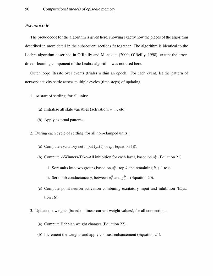
50 Computational models of episodic memory
Pseudocode
The pseudocode for the algorithm is given here, showing exactly how the pieces of the algorithm
described in more detail in the subsequent sections fit together. The algorithm is identical to the
Leabra algorithm described in O’Reilly and Munakata (2000; O’Reilly, 1998), except the error-
driven-learning component of the Leabra algorithm was not used here.
Outer loop: Iterate over events (trials) within an epoch. For each event, let the pattern of
network activity settle across multiple cycles (time steps) of updating:
1. At start of settling, for all units:
(a) Initialize all state variables (activation, v_m, etc).
(b) Apply external patterns.
2. During each cycle of settling, for all non-clamped units:
(a) Compute excitatory net input (ge(t) or ηj, Equation 18).
(b) Compute k-Winners-Take-All inhibition for each layer, based on gΘi (Equation 21):
i. Sort units into two groups based on gΘi : top k and remaining k + 1 to n.
ii. Set inhib conductance gi between gΘk and gΘ
k+1 (Equation 20).
(c) Compute point-neuron activation combining excitatory input and inhibition (Equa-
tion 16).
3. Update the weights (based on linear current weight values), for all connections:
(a) Compute Hebbian weight changes (Equation 22).
(b) Increment the weights and apply contrast-enhancement (Equation 24).

Norman, Detre, & Polyn 51
Point Neuron Activation Function
Leabra uses a point neuron activation function that models the electrophysiological properties
of real neurons, while simplifying their geometry to a single point.
The membrane potential Vm is updated as a function of ionic conductances g with reversal
(driving) potentials E as follows:
dVm(t)
dt= τ
∑
c
gc(t)gc(Ec − Vm(t)) (16)
with 3 channels (c) corresponding to: e excitatory input; l leak current; and i inhibitory input.
Following electrophysiological convention, the overall conductance is decomposed into a time-
varying component gc(t) computed as a function of the dynamic state of the network, and a constant
gc that controls the relative influence of the different conductances. The equilibrium potential can
be written in a simplified form by setting the excitatory driving potential (Ee) to 1 and the leak and
inhibitory driving potentials (El and Ei) of 0:
V ∞
m =gege
gege + glgl + gigi
(17)
which shows that the neuron is computing a balance between excitation and the opposing forces
of leak and inhibition.
The excitatory net input/conductance ge(t) or ηj is computed as the proportion of open excita-
tory channels as a function of sending activations times the weight values:
ηj = ge(t) = 〈xiwij〉 =1
n
∑
i
xiwij (18)
The inhibitory conductance is computed via the k-Winners-Take-All function described in the next
section, and leak is a constant.

52 Computational models of episodic memory
Activation communicated to other cells (yj) is a thresholded (Θ) sigmoidal function of the
membrane potential with gain parameter γ:
yj(t) =1
(
1 + 1γ[Vm(t)−Θ]+
) (19)
where [x]+ is a threshold function that returns 0 if x < 0 and x if X > 0. This sharply-thresholded
function is convolved with a Gaussian noise kernel (σ = .005), which reflects the intrinsic pro-
cessing noise of biological neurons.
k-Winners-Take-All Inhibition
Leabra uses a k-Winners-Take-All (kWTA) function to achieve sparse distributed representa-
tions (c.f., Minai & Levy, 1994). A uniform level of inhibitory current for all units in the layer is
computed as follows:
gi = gΘk+1 + q(gΘ
k − gΘk+1) (20)
where 0 < q < 1 is a parameter for setting the inhibition between the upper bound of gΘk and the
lower bound of gΘk+1. These boundary inhibition values are computed as a function of the level of
inhibition necessary to keep a unit right at threshold:
gΘi =
g∗
e ge(Ee − Θ) + glgl(El − Θ)
Θ − Ei
(21)
where g∗
e is the excitatory net input without the bias weight contribution — this allows the bias
weights to override the kWTA constraint.
In the basic version of the kWTA function used here, gΘk and gΘ
k+1 are set to the threshold
inhibition value for the k th and k + 1 th most excited units, respectively. Thus, the inhibition is
placed exactly to allow k units to be above threshold, and the remainder below threshold. For this
version, the q parameter is set to .25, allowing the k th unit to be sufficiently above the inhibitory

Norman, Detre, & Polyn 53
threshold.
Hebbian Learning
The simplest form of Hebbian learning adjusts the weights in proportion to the product of the
sending (xi) and receiving (yj) unit activations: ∆wij = xiyj. The weight vector is dominated by
the principal eigenvector of the pairwise correlation matrix of the input, but it also grows without
bound. Leabra uses essentially the same learning rule used in competitive learning or mixtures-of-
Gaussians (Rumelhart & Zipser, 1986; Nowlan, 1990; Grossberg, 1976), which can be seen as a
variant of the Oja normalization (Oja, 1982):
∆hebbwij = xiyj − yjwij = yj(xi − wij) (22)
Rumelhart and Zipser (1986) and O’Reilly and Munakata (2000) showed that, when activations are
interpreted as probabilities, this equation converges on the conditional probability that the sender
is active given that the receiver is active.
To renormalize Hebbian learning for sparse input activations, Equation 22 can be re-written as
follows:
∆wij = ε[yjxi(m − wij) + yj(1 − xi)(0 − wij)] (23)
where an m value of 1 gives Equation 22, while a larger value can ensure that the weight value
between uncorrelated but sparsely active units is around .5. In these simulations, m = .5αm
and
αm = .5 − qm(.5 − α), where α is the sending layer’s expected activation level, and qm (called
savg cor in the simulator) is the extent to which this sending layer’s average activation is fully
corrected for (qm = 1 gives full correction, and qm = 0 yields no correction).
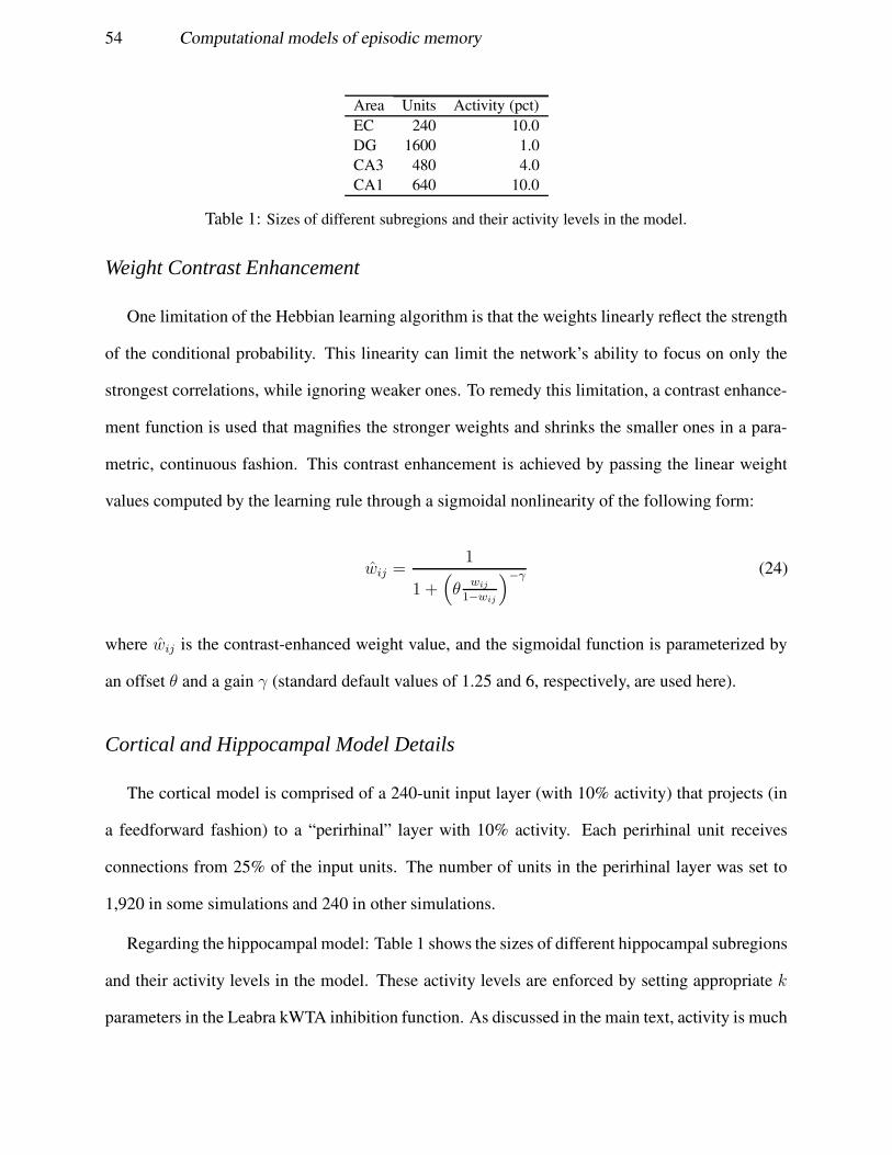
54 Computational models of episodic memory
Area Units Activity (pct)EC 240 10.0DG 1600 1.0CA3 480 4.0CA1 640 10.0
Table 1: Sizes of different subregions and their activity levels in the model.
Weight Contrast Enhancement
One limitation of the Hebbian learning algorithm is that the weights linearly reflect the strength
of the conditional probability. This linearity can limit the network’s ability to focus on only the
strongest correlations, while ignoring weaker ones. To remedy this limitation, a contrast enhance-
ment function is used that magnifies the stronger weights and shrinks the smaller ones in a para-
metric, continuous fashion. This contrast enhancement is achieved by passing the linear weight
values computed by the learning rule through a sigmoidal nonlinearity of the following form:
wij =1
1 +(
θwij
1−wij
)
−γ (24)
where wij is the contrast-enhanced weight value, and the sigmoidal function is parameterized by
an offset θ and a gain γ (standard default values of 1.25 and 6, respectively, are used here).
Cortical and Hippocampal Model Details
The cortical model is comprised of a 240-unit input layer (with 10% activity) that projects (in
a feedforward fashion) to a “perirhinal” layer with 10% activity. Each perirhinal unit receives
connections from 25% of the input units. The number of units in the perirhinal layer was set to
1,920 in some simulations and 240 in other simulations.
Regarding the hippocampal model: Table 1 shows the sizes of different hippocampal subregions
and their activity levels in the model. These activity levels are enforced by setting appropriate k
parameters in the Leabra kWTA inhibition function. As discussed in the main text, activity is much
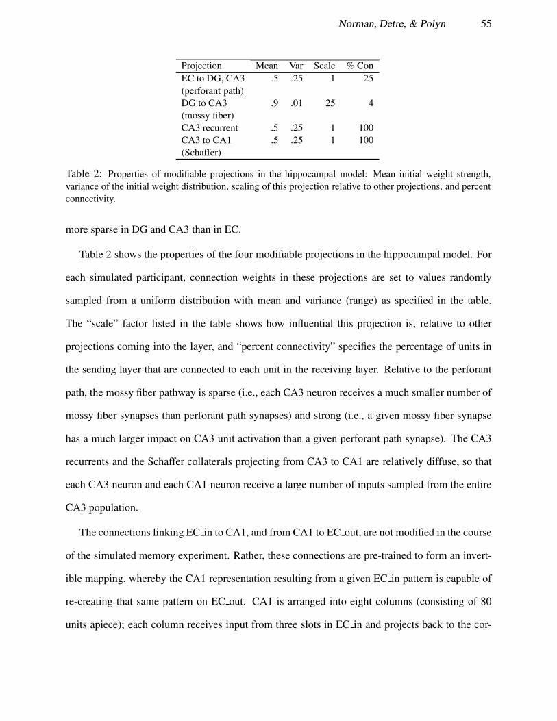
Norman, Detre, & Polyn 55
Projection Mean Var Scale % ConEC to DG, CA3 .5 .25 1 25(perforant path)DG to CA3 .9 .01 25 4(mossy fiber)CA3 recurrent .5 .25 1 100CA3 to CA1 .5 .25 1 100(Schaffer)
Table 2: Properties of modifiable projections in the hippocampal model: Mean initial weight strength,variance of the initial weight distribution, scaling of this projection relative to other projections, and percentconnectivity.
more sparse in DG and CA3 than in EC.
Table 2 shows the properties of the four modifiable projections in the hippocampal model. For
each simulated participant, connection weights in these projections are set to values randomly
sampled from a uniform distribution with mean and variance (range) as specified in the table.
The “scale” factor listed in the table shows how influential this projection is, relative to other
projections coming into the layer, and “percent connectivity” specifies the percentage of units in
the sending layer that are connected to each unit in the receiving layer. Relative to the perforant
path, the mossy fiber pathway is sparse (i.e., each CA3 neuron receives a much smaller number of
mossy fiber synapses than perforant path synapses) and strong (i.e., a given mossy fiber synapse
has a much larger impact on CA3 unit activation than a given perforant path synapse). The CA3
recurrents and the Schaffer collaterals projecting from CA3 to CA1 are relatively diffuse, so that
each CA3 neuron and each CA1 neuron receive a large number of inputs sampled from the entire
CA3 population.
The connections linking EC in to CA1, and from CA1 to EC out, are not modified in the course
of the simulated memory experiment. Rather, these connections are pre-trained to form an invert-
ible mapping, whereby the CA1 representation resulting from a given EC in pattern is capable of
re-creating that same pattern on EC out. CA1 is arranged into eight columns (consisting of 80
units apiece); each column receives input from three slots in EC in and projects back to the cor-
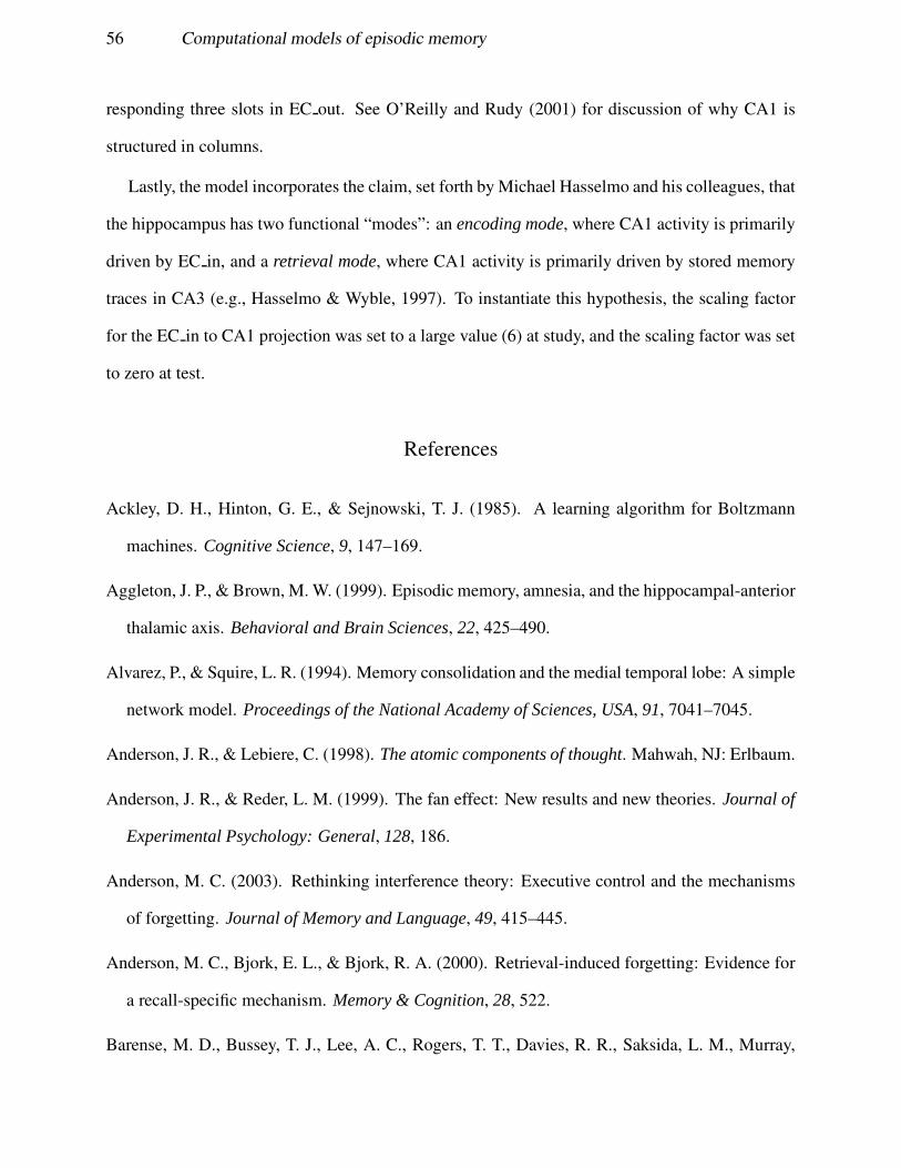
56 Computational models of episodic memory
responding three slots in EC out. See O’Reilly and Rudy (2001) for discussion of why CA1 is
structured in columns.
Lastly, the model incorporates the claim, set forth by Michael Hasselmo and his colleagues, that
the hippocampus has two functional “modes”: an encoding mode, where CA1 activity is primarily
driven by EC in, and a retrieval mode, where CA1 activity is primarily driven by stored memory
traces in CA3 (e.g., Hasselmo & Wyble, 1997). To instantiate this hypothesis, the scaling factor
for the EC in to CA1 projection was set to a large value (6) at study, and the scaling factor was set
to zero at test.
References
Ackley, D. H., Hinton, G. E., & Sejnowski, T. J. (1985). A learning algorithm for Boltzmann
machines. Cognitive Science, 9, 147–169.
Aggleton, J. P., & Brown, M. W. (1999). Episodic memory, amnesia, and the hippocampal-anterior
thalamic axis. Behavioral and Brain Sciences, 22, 425–490.
Alvarez, P., & Squire, L. R. (1994). Memory consolidation and the medial temporal lobe: A simple
network model. Proceedings of the National Academy of Sciences, USA, 91, 7041–7045.
Anderson, J. R., & Lebiere, C. (1998). The atomic components of thought. Mahwah, NJ: Erlbaum.
Anderson, J. R., & Reder, L. M. (1999). The fan effect: New results and new theories. Journal of
Experimental Psychology: General, 128, 186.
Anderson, M. C. (2003). Rethinking interference theory: Executive control and the mechanisms
of forgetting. Journal of Memory and Language, 49, 415–445.
Anderson, M. C., Bjork, E. L., & Bjork, R. A. (2000). Retrieval-induced forgetting: Evidence for
a recall-specific mechanism. Memory & Cognition, 28, 522.
Barense, M. D., Bussey, T. J., Lee, A. C., Rogers, T. T., Davies, R. R., Saksida, L. M., Murray,
Norman, Detre, & Polyn 57
E. A., & Graham, K. S. (2005). Functional specialization in the human medial temporal lobe.
Journal of Neuroscience, 25(44), 10239–46.
Barnes, J. M., & Underwood, B. J. (1959). Fate of first-list associations in transfer theory. Journal
of Experimental Psychology, 58, 97–105.
Becker, S. (2005). A computational principle for hippocampal learning and neurogenesis. Hip-
pocampus, 15(6), 722–38.
Becker, S., & Lim, J. (2003). A computational model of prefrontal control in free recall: strategic
memory use in the california verbal learning task. Journal of Cognitive Neuroscience, 15, 821–
832.
Bjork, R. A., & Whitten, W. B. (1974). Recency-sensitive retrieval processes in long-term free
recall. Cognitive Psychology, 6, 173–189.
Bogacz, R., & Brown, M. W. (2003). Comparison of computational models of familiarity discrim-
ination in the perirhinal cortex. Hippocampus, 13, 494–524.
Botvinick, M., & Plaut, D. C. (2006). Short-term memory for serial order: A recurrent neural
network model. Psychological Review, 113, 201–233.
Brainerd, C. J., & Reyna, V. F. (1998). When things that were never experienced are easier to
”remember” than things that were. Psychological Science, 9, 484.
Brozinsky, C. J., Yonelinas, A. P., Kroll, N. E., & Ranganath, C. (2005). Lag-sensitive repetition
suppression effects in the anterior parahippocampal gyrus. Hippocampus, 15, 557–561.
Burgess, N., Becker, S., King, J. A., & O’Keefe, J. (2001). Memory for events and their spatial
context: models and experiments. Philosophical Transactions of the Royal Society of London.
Series B, Biological Sciences, 356(1413), 1493–503.
Burgess, N., & Hitch, G. (2005). Computational models of working memory: putting long-term
memory into context. Trends in Cognitive Sciences, 9(11), 535–41.

58 Computational models of episodic memory
Burgess, N., & O’Keefe, J. (1996). Neuronal computations underlying the firing of place cells and
their role in navigation. Hippocampus, 6, 749–762.
Bussey, T. J., & Saksida, L. M. (2002). The organisation of visual object representations: A con-
nectionist model of effects of lesions in perirhinal cortex. European Journal of Neuroscience,
15, 355–364.
Bussey, T. J., Saksida, L. M., & Murray, E. A. (2002). The role of perirhinal cortex in memory
and perception: Conjunctive representations for object identification. In M. P. Witter, & F. G.
Waterlood (Eds.), The parahippocampal region: Organisation and role in cognitive functions.
New York: Oxford.
Carlesimo, G. A., Marfia, G. A., Loasses, A., & Caltagirone, C. (1996). Recency effect in antero-
grade amnesia: evidence for distinct memory stores underlying enhanced retrieval of terminal
items in immediate and delayed recall paradigms. Neuropsychologia, 34(3), 177–84.
Clark, S. E., & Gronlund, S. D. (1996). Global matching models of recognition memory: How the
models match the data. Psychonomic Bulletin and Review, 3, 37–60.
Criss, A. H., & Shiffrin, R. M. (2004). Context noise and item noise jointly determine recognition
memory: A comment on dennis and humphreys (2001). Psychological Review, 111, 800–807.
Davachi, L., Mitchell, J. P., & Wagner, A. D. (2003). Multiple routes to memory: distinct medial
temporal processes build item and source memories. Proceedings of the National Academy of
Sciences, 100, 2157–2162.
Davelaar, E. J., Goshen-Gottstein, Y., Ashkenazi, A., Haarmann, H. J., & Usher, M. (2005). The
demise of short-term memory revisited: Empirical and computational investigations of recency
effects. Psychological Review, 112, 3–42.
Deco, G., Rolls, E. T., & Horwitz, B. (2004). ”What” and ”where” in visual working memory:

Norman, Detre, & Polyn 59
a computational neurodynamical perspective. Journal of Cognitive Neuroscience, 16(4), 683–
701.
Dennis, S., & Humphreys, M. S. (2001). A context noise model of episodic word recognition.
Psychological Review, 108, 452–477.
Dobbins, I. G., Rice, H. J., Wagner, A. D., & Schacter, D. L. (2003). Memory orientation and suc-
cess: Separate neurocognitive components underlying episodic recognition. Neuropsychologia,
41, 318–333.
Durstewitz, D., Kelc, M., & Gunturkun, O. (1999). A neurocomputational theory of the dopamin-
ergic modulation of working memory functions. Journal of Neuroscience, 19, 2807.
Durstewitz, D., Seamans, J. K., & Sejnowski, T. J. (2000). Dopamine-mediated stabilization of
delay-period activity in a network model of prefrontal cortex. Journal of Neurophysiology, 83,
1733.
Egorov, A. V., Hamam, B. N., Fransen, E., Hasselmo, M. E., & Alonso, A. A. (2002). Graded
persistent activity in entorhinal cortex neurons. Nature, 420, 173–8.
Eichenbaum, H., H., Otto, T., & Cohen, N. J. (1994). Two functional components of the hippocam-
pal memory system. Behavioral and Brain Sciences, 17(3), 449–518.
Eldridge, L. L., Knowlton, B. J., Furmanski, C. S., Bookheimer, S. Y., & Engel, S. A. (2000).
Remembering episodes: a selective role for the hippocampus during retrieval. Nature Neuro-
science, 3, 1149–52.
Elman, J. L. (1991). Distributed representations, simple recurrent networks, and grammatical
structure. Machine Learning, 7, 195–225.
Estes, W. K. (1955). Statistical theory of distributional phenomena in learning. Psychological
Review, 62, 369–377.
60 Computational models of episodic memory
Fellous, J. M., Wang, X. J., & Lisman, J. E. (1998). A role for NMDA-receptor channels in
working memory. Nature Neuroscience, 1, 273–275.
Ferino, F., Thierry, A. M., & Glowinski, J. (1987). Anatomical and electrophysiological evidence
for a direct projection from ammon’s horn to the medial prefrontal cortex in the rat. Experimen-
tal Brain Research, 65, 421–426.
Fletcher, P. C., & Henson, R. N. (2001). Frontal lobes and human memory: insights from functional
neuroimaging. Brain, 124(Pt 5), 849–81.
Fortin, N. J., Wright, S. P., & Eichenbaum, H. B. (2004). Recollection-like memory retrieval in
rats is dependent on the hippocampus. Nature, 431, 188–191.
Frank, M. J., Loughry, B., & O’Reilly, R. C. (2001). Interactions between the frontal cortex and
basal ganglia in working memory: A computational model. Cognitive, Affective, and Behavioral
Neuroscience, 1, 137–160.
Gillund, G., & Shiffrin, R. M. (1984). A retrieval model for both recognition and recall. Psycho-
logical Review, 91, 1–67.
Glanzer, M., Adams, J. K., Iverson, G. J., & Kim, K. (1993). The regularities of recognition
memory. Psychological Review, 100, 546–567.
Glenberg, A. M., Bradley, M. M., Stevenson, J. A., Kraus, T. A., Tkachuk, M. J., Gretz, A. L.,
Fish, J. H., & Turpin, B. M. (1980). A two-process account of long-term serial position effects.
Journal of Experimental Psychology: Learning, Memory, and Cognition, 6, 355–369.
Gluck, M. A., Meeter, M., & Myers, C. E. (2003). Computational models of the hippocampal
region: linking incremental learning and episodic memory. Trends in Cognitive Sciences, 7(6),
269–276.
Goldman-Rakic, P. S., Selemon, L. D., & Schwartz, M. L. (1984). Dual pathways connecting the
Norman, Detre, & Polyn 61
dorsolateral prefrontal cortex with the hippocampal formation and parahippocampal cortex in
the rhesus monkey. Neuroscience, 12, 719–743.
Gonsalves, B. D., Kahn, I., Curran, T., Norman, K. A., & Wagner, A. D. (2005). Memory strength
and repetition suppression: Multimodal imaging of medial temporal contributions to recogni-
tion. Neuron, 47, 751–761.
Grossberg, S. (1976). Adaptive pattern classification and universal recoding I: Parallel develop-
ment and coding of neural feature detectors. Biological Cybernetics, 23, 121–134.
Grossberg, S. (1986). The adaptive self-organization of serial order in behavior: Speech, language,
and motor control. In E. C. Scwab, & H. C. Nusbaum (Eds.), Pattern recognition in humans
and machines, volume I: Speech perception. New York: Academic Press.
Grossberg, S., & Stone, G. (1986). Neural dynamics of word recognition and recall: Attentional
priming, learning, and resonance. Psychological Review, 93, 46–74.
Gruppuso, V., Lindsay, D. S., & Kelley, C. M. (1997). The process-dissociation procedure and
similarity: Defining and estimating recollection and familiarity in recognition memory. Journal
of Experimental Psychology: Learning, Memory, and Cognition, 23, 259.
Hasselmo, M. E. (1995). Neuromodulation and cortical function: Modeling the physiological basis
of behavior. Behavioural Brain Research, 67, 1–27.
Hasselmo, M. E., Bodelon, C., & Wyble, B. P. (2002). A proposed function for hippocampal theta
rhythm: Separate phases of encoding and retrieval enhance reversal of prior learning. Neural
Computation, 14, 793–818.
Hasselmo, M. E., & Fehlau, B. P. (2001). Differences in time course of ACh and GABA modulation
of excitatory synaptic potentials in slices of rat hippocampus. Journal of Neurophysiology,
86(4), 1792–802.
Hasselmo, M. E., & Schnell, E. (1994). Laminar selectivity of the cholinergic suppression of

62 Computational models of episodic memory
synaptic transmission in rat hippocampal region CA1: computational modeling and brain slice
physiology. Journal of Neuroscience, 14(6), 3898–914.
Hasselmo, M. E., Schnell, E., & Barkai, E. (1995). Dynamics of learning and recall at excitatory
recurrent synapses and cholinergic modulation in rat hippocampal region CA3. Journal of
Neuroscience, 15(7 Pt 2), 5249–62.
Hasselmo, M. E., & Wyble, B. (1997). Free recall and recognition in a network model of the
hippocampus: Simulating effects of scopolamine on human memory function. Behavioural
Brain Research, 89, 1–34.
Hasselmo, M. E., Wyble, B., & Wallenstein, G. V. (1996). Encoding and retrieval of episodic
memories: Role of cholinergic and GABAergic modulation in the hippocampus. Hippocampus,
6, 693–708.
Henson, R. N. A., Cansino, S., Herron, J. E., Robb, W. G., & Rugg, M. D. (2003). A familiarity
signal in human anterior medial temporal cortex? Hippocampus, 13, 301–304.
Hinton, G. E. (1989). Deterministic Boltzmann learning performs steepest descent in weight-space.
Neural Computation, 1, 143–150.
Hinton, G. E., & Sejnowski, T. J. (1986). Learning and relearning in Boltzmann machines. In D. E.
Rumelhart, J. L. McClelland, & PDP Research Group (Eds.), Parallel distributed processing.
Volume 1: Foundations (Chap. 7, pp. 282–317). Cambridge, MA: MIT Press.
Hintzman, D. L. (1988). Judgments of frequency and recognition memory in a multiple-trace
memory model. Psychological Review, 95, 528–551.
Hintzman, D. L., Curran, T., & Oppy, B. (1992). Effects of similiarity and repetition on memory:
Registration without learning. Journal of Experimental Psychology: Learning, Memory, and
Cognition, 18, 667–680.
Hirshman, E., Fisher, J., Henthorn, T., Arndt, J., & Passannante, A. (2002). Midazolam amnesia

Norman, Detre, & Polyn 63
and dual-process models of the word-frequency mirror effect. Journal of Memory and Lan-
guage, 47, 499–516.
Holdstock, J. S., Mayes, A. R., Roberts, N., Cezayirli, E., Isaac, C. L., O’Reilly, R. C., & Norman,
K. A. (2002). Under what conditions is recognition spared relative to recall after selective
hippocampal damage in humans? Hippocampus, 12, 341–351.
Howard, M. W., Addis, K. M., Jing, B., & Kahana, M. J. (in press-a). Semantic structure and
episodic memory. In T. Landauer, D. McNamara, S. Dennis, & W. Kintsch (Eds.), LSA: A road
towards meaning. Mahwah, NJ: Lawrence Erlbaum.
Howard, M. W., Fotedar, M. S., Datey, A. V., & Hasselmo, M. E. (2005). The temporal context
model in spatial navigation and relational learning: Toward a common explanation of medial
temporal lobe function across domains. Psychological Review, 112, 75–116.
Howard, M. W., & Kahana, M. J. (1999). Contextual variability and serial position effects in free
recall. Journal of Experimental Psychology: Learning, Memory, and Cognition, 25, 923.
Howard, M. W., & Kahana, M. J. (2002). A distributed representation of temporal context. Journal
of Mathematical Psychology, 46, 269–299.
Howard, M. W., Kahana, M. J., & Wingfield, A. (in press-b). Aging and contextual binding:
Modeling recency and lag-recency effects within the temporal context model. Psychonomic
Bulletin and Review.
Humphreys, M. S., Bain, J. D., & Pike, R. (1989). Different ways to cue a coherent memory
system: A theory for episodic, semantic, and procedural tasks. Psychological Review, 96, 208–
233.
Jacoby, L. L., Yonelinas, A. P., & Jennings, J. M. (1997). The relation between conscious and
unconscious (automatic) influences: A declaration of independence. In J. D. Cohen, & J. W.
64 Computational models of episodic memory
Schooler (Eds.), Scientific approaches to consciousness (pp. 13–47). Mahway, NJ: Lawrence
Erlbaum Associates.
Jay, T. M., & Witter, M. P. (1991). Distribution of hippocampal CA1 and subicular efferents in
the prefrontal cortex of the rat studied by means of anterograde transport of phaseolus vulgaris-
leucoagglutinin. The Journal of Comparative Neurology, 313, 574–586.
Jensen, O., & Lisman, J. E. (2005). Hippocampal sequence-encoding driven by a cortical multi-
item working memory buffer. Trends in Neurosciences, 28(2), 67–72.
Joordens, S., & Hockley, W. E. (2000). Recollection and familiarity through the looking glass:
When old does not mirror new. Journal of Experimental Psychology: Learning, Memory, and
Cognition, 26, 1534.
Kahana, M. J. (1996). Associative retrieval processes in free recall. Memory and Cognition, 24,
103–109.
Kahana, M. J., & Sekuler, R. (2002). Recognizing spatial patterns: A noisy exemplar approach.
Vision Research, 42, 2177–92.
Koutstaal, W., Schacter, D. L., & Jackson, E. M. (1999). Perceptually based false recognition
of novel objects in amnesia: Effects of category size and similarity to category prototypes.
Cognitive Neuropsychology, 16, 317.
Levitt, J. B., Lewis, D. A., Yoshioka, T., & Lund, J. S. (1993). Topography of pyramidal neuron
intrinsic connections in macaque monkey prefrontal cortex (areas 9 & 46). Journal of Compar-
ative Neurology, 338, 360–376.
Li, L., Miller, E. K., & Desimone, R. (1993). The representation of stimulus familiarity in anterior
inferior temporal cortex. Journal of Neurophysiology, 69, 1918–1929.
Malmberg, K. J., Holden, J. E., & Shiffrin, R. M. (2004a). Modeling the effects of repetitions,

Norman, Detre, & Polyn 65
similarity, and normative word frequency on old-new recognition and judgments of frequency.
Journal of Experimental Psychology: Learning, Memory, and Cognition, 30(2), 319–31.
Malmberg, K. J., & Shiffrin, R. M. (2005). The ’one-shot’ hypothesis for context storage. Journal
of Experimental Psychology: Learning, Memory, and Cognition, 31(2), 322–36.
Malmberg, K. J., & Xu, J. (in press). On the flexibility and fallibility of associative memory.
Memory and Cognition.
Malmberg, K. J., Zeelenberg, R., & Shiffrin, R. M. (2004b). Turning up the noise or turning down
the volume? on the nature of the impairment of episodic recognition memory by midazolam.
Journal of Experimental Psychology. Learning, Memory, and Cognition, 30(2), 540–9.
Manns, J. R., Hopkins, R. O., Reed, J. M., Kitchener, E. G., & Squire, L. R. (2003). Recognition
memory and the human hippocampus. Neuron, 37, 171–180.
Marr, D. (1971). Simple memory: A theory for archicortex. Philosophical Transactions of the
Royal Society (London) B, 262, 23–81.
Mayes, A. R., Isaac, C. L., Downes, J. J., Holdstock, J. S., Hunkin, N. M., Montaldi, D., Mac-
Donald, C., Cezayirli, E., & Roberts, J. N. (2001). Memory for single items, word pairs, and
temporal order in a patient with selective hippocampal lesions. Cognitive Neuropsychology, 18,
97–123.
McClelland, J. L., & Chappell, M. (1998). Familiarity breeds differentiation: a subjective-
likelihood approach to the effects of experience in recognition memory. Psychological Review,
105, 724.
McClelland, J. L., & Goddard, N. H. (1996). Considerations arising from a complementary learn-
ing systems perspective on hippocampus and neocortex. Hippocampus, 6, 654–665.
McClelland, J. L., McNaughton, B. L., & O’Reilly, R. C. (1995). Why there are complementary

66 Computational models of episodic memory
learning systems in the hippocampus and neocortex: Insights from the successes and failures of
connectionist models of learning and memory. Psychological Review, 102, 419–457.
McNaughton, B. L., & Morris, R. G. M. (1987). Hippocampal synaptic enhancement and infor-
mation storage within a distributed memory system. Trends in Neurosciences, 10(10), 408–415.
Meeter, M., & Murre, J. (in press). Tracelink: A model of amnesia and consolidation. Cognitive
Neuropsychology.
Meeter, M., Murre, J., & Talamini, L. M. (2004). Mode shifting between storage and recall based
on novelty detection in oscillating hippocampal circuits. Hippocampus, 14, 722–741.
Meeter, M., Myers, C. E., & Gluck, M. A. (2005). Integrating incremental learning and episodic
memory models of the hippocampal region. Psychological Review, 112, 560–85.
Mehta, M. R., Lee, A. K., & Wilson, M. A. (2002). Role of experience and oscillations in trans-
forming a rate code into a temporal code. Nature, 416, 741–745.
Melton, A. W., & Irwin, J. M. (1940). The influence of degree of interpolated learning on retroac-
tive inhibition and the overt transfer of specific responses. American Journal of Psychology, 3,
173–203.
Mensink, G., & Raaijmakers, J. G. (1988). A model for interference and forgetting. Psychological
Review, 95, 434–455.
Minai, A. A., & Levy, W. B. (1994). Setting the activity level in sparse random networks. Neural
Computation, 6, 85–99.
Moll, M., & Miikkulainen, R. (1997). Convergence-zone episodic memory: Analysis and simula-
tions. Neural Networks, 10, 1017–1036.
Morris, R., Pandya, D. N., & Petrides, M. (1999). Fiber system linking the mid-dorsolateral
frontal cortex with the retrosplenial/presubicular region in the rhesus monkey. The Journal of
Comparative Neurology, 407, 183–192.

Norman, Detre, & Polyn 67
Movellan, J. R. (1990). Contrastive Hebbian learning in the continuous Hopfield model. In D. S.
Tourtezky, G. E. Hinton, & T. J. Sejnowski (Eds.), Proceedings of the 1989 Connectionist Mod-
els Summer School (pp. 10–17).
Murdock, B. B. (1993). TODAM2: A model for the storage and retrieval of item, associative, and
serial-order information. Psychological Review, 100, 183–203.
Murnane, K., & Shiffrin, R. (1991). Interference and the representation of events in memory.
Journal of Experimental Psychology: Learning, Memory, and Cognition, 17, 855–874.
Norman, K. A., Newman, E. L., & Detre, G. J. (2006a). A neural network model of retrieval-
induced forgetting (Technical Report 06-1). Princeton, NJ: Princeton University, Center for the
Study of Brain, Mind, and Behavior.
Norman, K. A., Newman, E. L., Detre, G. J., & Polyn, S. M. (2006b). How inhibitory oscillations
can train neural networks and punish competitors. Neural Computation, 18, 1577–610.
Norman, K. A., Newman, E. L., & Perotte, A. J. (2005). Methods for reducing interference in
the complementary learning systems model: Oscillating inhibition and autonomous memory
rehearsal. Neural Networks, 18, 1212–1228.
Norman, K. A., & O’Reilly, R. C. (2003). Modeling hippocampal and neocortical contributions
to recognition memory: A complementary-learning-systems approach. Psychological Review,
104, 611–646.
Nowlan, S. J. (1990). Maximum likelihood competitive learning. In D. S. Touretzky (Ed.), Ad-
vances in neural information processing systems, 2 (pp. 574–582). San Mateo, CA: Morgan
Kaufmann.
Oja, E. (1982). A simplified neuron model as a principal component analyzer. Journal of Mathe-
matical Biology, 15, 267–273.

68 Computational models of episodic memory
O’Keefe, J., & Nadel, L. (1978). The hippocampus as a cognitive map. Oxford, England: Oxford
University Press.
O’Reilly, R. C. (1998). Six principles for biologically-based computational models of cortical
cognition. Trends in Cognitive Sciences, 2(11), 455–462.
O’Reilly, R. C., & Frank, M. J. (2006). Making working memory work: A computational model
of learning in the frontal cortex and basal ganglia. Neural Computation, 18, 283–328.
O’Reilly, R. C., & McClelland, J. L. (1994). Hippocampal conjunctive encoding, storage, and
recall: Avoiding a tradeoff. Hippocampus, 4(6), 661–682.
O’Reilly, R. C., & Munakata, Y. (2000). Computational explorations in cognitive neuroscience:
Understanding the mind by simulating the brain. Cambridge, MA: MIT Press.
O’Reilly, R. C., Norman, K. A., & McClelland, J. L. (1998). A hippocampal model of recognition
memory. In M. I. Jordan, M. J. Kearns, & S. A. Solla (Eds.), Advances in neural information
processing systems 10 (pp. 73–79). Cambridge, MA: MIT Press.
O’Reilly, R. C., & Rudy, J. W. (2001). Conjunctive representations in learning and memory:
Principles of cortical and hippocampal function. Psychological Review, 108, 311–345.
Peterson, L. R., & Peterson, M. R. (1959). Short-term retention of individual verbal items. Journal
of Experimental Psychology, 58, 193–198.
Polyn, S. M. (2005). Neuroimaging, behavioral, and computational investigations of memory
targeting. PhD thesis, Princeton University, Princeton, New Jersey, USA.
Polyn, S. M., Norman, K. A., & Cohen, J. D. (2003, April). Modeling prefrontal and medial
temporal contributions to episodic memory. 10th Annual Meeting of the Cognitive Neuroscience
Society.
Pucak, M. L., Levitt, J. B., Lund, J. S., & Lewis, D. A. (1996). Patterns of intrinsic and associa-
tional circuitry in monkey prefrontal cortex. Journal of Comparative Neurology, 376, 614–630.
Norman, Detre, & Polyn 69
Raaijmakers, J. G. W. (2005). Modeling implicit and explicit memory. In C. Izawa, & N. Ohta
(Eds.), Human learning and memory: Advances in theory and application (pp. 85–105). Mah-
wah, NJ: Erlbaum.
Raaijmakers, J. G. W., & Shiffrin, R. M. (1981). Search of associative memory. Psychological
Review, 88, 93–134.
Raaijmakers, J. G. W., & Shiffrin, R. M. (2002). Models of memory. In H. Pashler, & D. Medin
(Eds.), Stevens’ handbook of experimental psychology, Third edition, Volume 2: Memory and
cognitive processes (pp. 43–76). New York: John Wiley and Sons.
Ranganath, C., Yonelinas, A. P., Cohen, M. X., Dy, C. J., Tom, S., & D’Esposito, M. (2003).
Dissociable correlates for familiarity and recollection within the medial temporal lobes. Neu-
ropsychologia, 42, 2–13.
Reder, L. M., Nhouyvanisvong, A., Schunn, C. D., Ayers, M. S., Angstadt, P., & Hiraki, K. A.
(2000). A mechanistic account of the mirror effect for word frequency: A computational model
of remember-know judgments in a continuous recognition paradigm. Journal of Experimental
Psychology: Learning, Memory, and Cognition, 26, 294–320.
Rolls, E. T. (1989). Functions of neuronal networks in the hippocampus and neocortex in memory.
In J. H. Byrne, & W. O. Berry (Eds.), Neural models of plasticity: Experimental and theoretical
approaches (pp. 240–265). San Diego, CA: Academic Press.
Rumelhart, D. E., & Zipser, D. (1986). Feature discovery by competitive learning. In D. E.
Rumelhart, J. L. McClelland, & PDP Research Group (Eds.), Parallel distributed processing.
Volume 1: Foundations (Chap. 5, pp. 151–193). Cambridge, MA: MIT Press.
Russchen, F. T., Amaral, D. G., & Price, J. L. (1987). The afferent input to the magnocellular
division of the mediodorsal thalamic nucleus in the monkey, macaca fascicularis. The Journal
of Comparative Neuroanatomy, 256, 175–210.

70 Computational models of episodic memory
Schacter, D. L. (1987). Memory, amnesia, and frontal lobe dysfunction. Psychobiology, 15, 21–36.
Scoville, W. B., & Milner, B. (1957). Loss of recent memory after bilateral hippocampal lesions.
Journal of Neurology, Neurosurgery, and Psychiatry, 20, 11–21.
Sherry, D. F., & Schacter, D. L. (1987). The evolution of multiple memory systems. Psychological
Review, 94(4), 439–454.
Shiffrin, R. M., Huber, D. E., & Marinelli, K. (1995). Effects of category length and strength
on familiarity in recognition. Journal of Experimental Psychology: Learning, Memory and
Cognition, 21, 267–287.
Shiffrin, R. M., & Steyvers, M. (1997). A model for recognition memory: REM – retrieving
effectively from memory. Psychonomic Bulletin and Review, 4, 145–166.
Shimamura, A. P. (1994). Memory and frontal lobe function. In M. S. Gazzaniga (Ed.), The
cognitive neurosciences (pp. 803–815). Cambridge, MA: MIT Press.
Simons, J. S., & Spiers, H. J. (2003). Prefrontal and medial temporal lobe interactions in long-term
memory. Nature Reviews Neuroscience, 4(8), 637–48.
Sohal, V. S., & Hasselmo, M. E. (2000). A model for experience-dependent changes in the re-
sponses of inferotemporal neurons. Network : Computation in Neural Systems, 11, 169.
Sohn, M. H., Goode, A., Stenger, V. A., Jung, K. J., Carter, C. S., & Anderson, J. R. (2005). An
information-processing model of three cortical regions: evidence in episodic memory retrieval.
Neuroimage, 25(1), 21–33.
Squire, L. R. (1992). Memory and the hippocampus: A synthesis from findings with rats, monkeys,
and humans. Psychological Review, 99, 195–231.
Squire, L. R., Shimamura, A. P., & Amaral, D. G. (1989). Memory and the hippocampus. In
J. H. Byrne, & W. O. Berry (Eds.), Neural models of plasticity: Experimental and theoretical
approaches (pp. 208–239). San Diego, CA: Academic Press.
Norman, Detre, & Polyn 71
Standing, L. (1973). Learning 10,000 pictures. Quarterly Journal of Experimental Psychology,
25, 207–222.
Sutherland, R. J., & Rudy, J. W. (1989). Configural association theory: The role of the hippocampal
formation in learning, memory, and amnesia. Psychobiology, 17(2), 129–144.
Teyler, T. J., & Discenna, P. (1986). The hippocampal memory indexing theory. Behavioral
Neuroscience, 100, 147–154.
Treves, A., & Rolls, E. T. (1994). A computational analysis of the role of the hippocampus in
memory. Hippocampus, 4, 374–392.
Usher, M., & Cohen, J. D. (1999). Short-term memory and selection processes in a frontal-lobe
model. In D. Heinke, G. W. Humphries, & A. Olsen (Eds.), Connectionist models in cognitive
neuroscience (pp. 78–91). London: Springer-Verlag.
Usher, M., & McClelland, J. L. (2001). The time course of perceptual choice: The leaky, competing
accumulator model. Psychological Review, 108, 550–592.
Westerberg, C. E., Paller, K. A., Weintraub, S., Mesulam, M. M., Holdstock, J., Mayes, A., &
Reber, P. J. (2006). When memory does not fail: Familiarity-based recognition in mild cognitive
impairment and alzheimer’s disease. Neuropsychology, 20, 193–205.
Witter, M. P., Wouterlood, F. G., Naber, P. A., & Van Haeften, T. (2000). Anatomical organization
of the parahippocampal-hippocampal network. Ann. N. Y. Acad. Sci., 911, 1–24.
Wu, X., Baxter, R. A., & Levy, W. B. (1996). Context codes and the effect of noisy learning on a
simplified hippocampal CA3 model. Biological Cybernetics, 74, 159–165.
Wyble, B. P., Linster, C., & Hasselmo, M. E. (2000). Size of CA1-evoked synaptic potentials is
related to theta rhythm phase in rat hippocampus. Journal of Neurophysiology, 83(4), 2138–44.
Xiang, J. Z., & Brown, M. W. (1998). Differential encoding of novelty, familiarity, and recency in
regions of the anterior temporal lobe. Neuropharmacology, 37, 657–676.

72 Computational models of episodic memory
Xu, J., & Malmberg, K. J. (in press). Modeling the effects of verbal- and non-verbal pair strength
on associative recognition. Memory and Cognition.
Yonelinas, A. P. (2002). The nature of recollection and familiarity: A review of 30 years of
research. Journal of Memory and Language, 46, 441–517.
Yonelinas, A. P., Kroll, N. E., Quamme, J. R., Lazzara, M. M., Sauve, M. J., Widaman, K. F., &
Knight, R. T. (2002). Effects of extensive temporal lobe damage or mild hypoxia on recollection
and familiarity. Nature Neuroscience, 5(11), 1236–1241.