
Computational Modelling of Artificial Language … · Computational Modelling of Artificial...
158
Computational Modelling of Artificial Language Learning: R etention, R ecognition & R ecurrence R aquel Garrido Alhama
-
Upload
hoangkhanh -
Category
Documents
-
view
221 -
download
0
Transcript of Computational Modelling of Artificial Language … · Computational Modelling of Artificial...

Computational Modelling
of Artificial Language Learning:
R etention, R ecognition & R ecurrence
R aquel Garrido Alhama

Computational Modelling
of Artificial Language Learning:
R etention, R ecognition & R ecurrence

ILLC Dissertation Series DS-2017-08
For further information about ILLC-publications, please contact
Institute for Logic, Language and ComputationUniversiteit van Amsterdam
Science Park 1071098 XG Amsterdam
phone: +31-20-525 6051e-mail: [email protected]
homepage: http://www.illc.uva.nl/
The investigations were supported by a grant from the Netherlands Organisation forScientific Research (NWO), Division of Humanities, to Levelt, ten Cate and Zuidema(NWO-GW 360.70.452).
Copyright c© 2017 by Raquel Garrido Alhama.Cover design by Roki.Printed and bound by Ridderprint.
ISBN: 978-94-6299-786-8
Computational Modelling
of Artificial Language Learning:
R etention, R ecognition & R ecurrence
ACADEMISCH PROEFSCHRIFT
ter verkrijging van de graad van doctoraan de Universiteit van Amsterdamop gezag van de Rector Magnificus
prof. dr. ir. K.I.J. Maexten overstaan van een door het College voor Promoties ingestelde
commissie, in het openbaar te verdedigen in de Aula der Universiteitop woensdag 29 november 2017, te 13.00 uur
door
Raquel Garrido Alhama
geboren te Artes, Spanje

Promotiecommisie
Promotor: Prof. Dr. C. J. ten Cate Universiteit van LeidenCo-promotor: Dr. W.H. Zuidema Universiteit van Amsterdam
Overige leden: Prof. Dr. K. Sima’an Universiteit van AmsterdamProf. Dr. H. Honing Universiteit van AmsterdamDr. A. Alishahi Universiteit van TilburgProf. Dr. P. Monaghan University of LancasterDr. J. E. Rispens Universiteit van Amsterdam
Faculteit der Natuurwetenschappen, Wiskunde en Informatica

And we know what we’re knowin’But we can’t say what we’ve seen
Talking Heads, Road to Nowhere
v


Contents
Acknowledgments xi
1 Introduction 11.1 Motivation . . . . . . . . . . . . . . . . . . . . . . . . . . . . . . . . 11.2 Outline . . . . . . . . . . . . . . . . . . . . . . . . . . . . . . . . . 4
2 Background 92.1 What is a computational model? . . . . . . . . . . . . . . . . . . . . 92.2 Marr’s levels of analysis . . . . . . . . . . . . . . . . . . . . . . . . 102.3 Families of Cognitive Models . . . . . . . . . . . . . . . . . . . . . . 13
2.3.1 Symbolic models . . . . . . . . . . . . . . . . . . . . . . . . 132.3.2 Exemplar-based Models . . . . . . . . . . . . . . . . . . . . 142.3.3 Bayesian Models . . . . . . . . . . . . . . . . . . . . . . . . 152.3.4 Connectionist models . . . . . . . . . . . . . . . . . . . . . . 17
2.4 What constitutes a good model? . . . . . . . . . . . . . . . . . . . . 19
I Segmentation 21
3 Segmentation as Retention and Recognition 233.1 Introduction . . . . . . . . . . . . . . . . . . . . . . . . . . . . . . . 233.2 Overview of the experimental record . . . . . . . . . . . . . . . . . . 243.3 R&R: the Retention-Recognition Model . . . . . . . . . . . . . . . . 26
3.3.1 Model description . . . . . . . . . . . . . . . . . . . . . . . 263.3.2 Qualitative behaviour of the model . . . . . . . . . . . . . . . 28
3.4 Predictions and empirical data . . . . . . . . . . . . . . . . . . . . . 303.4.1 Prediction of observed skew in response distribution in rats . . 303.4.2 Prediction of observed skew in response distribution in humans 323.4.3 Fitting R&R to forced choice data . . . . . . . . . . . . . . . 35
vii
3.5 Conclusions . . . . . . . . . . . . . . . . . . . . . . . . . . . . . . . 39
4 Model evaluation 414.1 Introduction . . . . . . . . . . . . . . . . . . . . . . . . . . . . . . . 414.2 Models of Segmentation . . . . . . . . . . . . . . . . . . . . . . . . 424.3 Existing evaluation procedures . . . . . . . . . . . . . . . . . . . . . 44
4.3.1 Evaluation based on the internal representations . . . . . . . . 444.3.2 Evaluation based on behavioural responses . . . . . . . . . . 45
4.4 Comparing alternative models against empirical data . . . . . . . . . 474.5 A proposal: evaluation over response distributions . . . . . . . . . . . 494.6 Conclusions . . . . . . . . . . . . . . . . . . . . . . . . . . . . . . . 51
II Propensity to Generalize 55
5 Modelling the Propensity to Generalize 575.1 Introduction . . . . . . . . . . . . . . . . . . . . . . . . . . . . . . . 575.2 Experimental Record . . . . . . . . . . . . . . . . . . . . . . . . . . 585.3 Understanding the generalization mechanism:
a three-step approach . . . . . . . . . . . . . . . . . . . . . . . . . . 615.4 Memorization of segments . . . . . . . . . . . . . . . . . . . . . . . 625.5 Quantifying the propensity to generalize . . . . . . . . . . . . . . . . 63
5.5.1 The Simple Good-Turing method . . . . . . . . . . . . . . . 635.5.2 Prediction of observed decrease in the propensity to generalize 65
5.6 Discussion . . . . . . . . . . . . . . . . . . . . . . . . . . . . . . . . 66
III Generalization 69
6 Computational Models of Rule Learning 716.1 Introduction . . . . . . . . . . . . . . . . . . . . . . . . . . . . . . . 716.2 The Empirical Data . . . . . . . . . . . . . . . . . . . . . . . . . . . 726.3 The Neural Network Models . . . . . . . . . . . . . . . . . . . . . . 74
6.3.1 The Simple Recurrent Network Models . . . . . . . . . . . . 746.3.2 Neural Networks with non-sequential input . . . . . . . . . . 796.3.3 Neural Networks with a repetition detector . . . . . . . . . . 816.3.4 Evaluating the Neural Network Models . . . . . . . . . . . . 84
6.4 Symbolic Models of Rule Learning . . . . . . . . . . . . . . . . . . . 856.5 Analysis of the Models . . . . . . . . . . . . . . . . . . . . . . . . . 87
6.5.1 Question 1: Which features or perceptual units participate inthe process? . . . . . . . . . . . . . . . . . . . . . . . . . . . 87
6.5.2 Question 2: What is the learning process? . . . . . . . . . . . 906.5.3 Question 3: Which generalization? . . . . . . . . . . . . . . . 90
viii
6.5.4 Question 4: What are the mental representations created? . . . 916.5.5 Conclusion of the analysis . . . . . . . . . . . . . . . . . . . 92
6.6 An agenda for Rule Learning . . . . . . . . . . . . . . . . . . . . . . 936.7 Conclusions . . . . . . . . . . . . . . . . . . . . . . . . . . . . . . . 96
7 Generalization in neural networks. 997.1 Introduction . . . . . . . . . . . . . . . . . . . . . . . . . . . . . . . 997.2 Background . . . . . . . . . . . . . . . . . . . . . . . . . . . . . . . 100
7.2.1 Empirical Data . . . . . . . . . . . . . . . . . . . . . . . . . 1007.2.2 Generalization and Neural Networks . . . . . . . . . . . . . . 101
7.3 Simulations with a Simple Recurrent Network . . . . . . . . . . . . . 1027.4 Simulations with an Echo State Network . . . . . . . . . . . . . . . . 1037.5 Pre-Wiring: Delay Line Memory . . . . . . . . . . . . . . . . . . . . 1057.6 Pre-Training: Incremental-Novelty Exposure . . . . . . . . . . . . . 1077.7 Discussion: Relation with other neural network techniques . . . . . . 108
7.7.1 Relation with Recurrent Neural Networks . . . . . . . . . . . 1087.7.2 Relation with standard Echo State Network . . . . . . . . . . 1097.7.3 Pre-Wiring: Relation with LSTMs . . . . . . . . . . . . . . . 1107.7.4 Pre-training: Relation with Dropout . . . . . . . . . . . . . . 111
7.8 Conclusion . . . . . . . . . . . . . . . . . . . . . . . . . . . . . . . 111
8 Conclusions 1158.1 Summary . . . . . . . . . . . . . . . . . . . . . . . . . . . . . . . . 1158.2 Contributions I: Exploring better ways to evaluate models . . . . . . . 1168.3 Contributions II: Exploring complementary levels of analysis . . . . . 1168.4 Contributions III: Reframing key theoretical debates . . . . . . . . . . 1178.5 Future work . . . . . . . . . . . . . . . . . . . . . . . . . . . . . . . 118
Samenvatting 133
Abstract 135
Curriculum Vitae 137
ix


Acknowledgments
This adventure started when Jelle, Remko, Carel and Claartje offered me a PhD po-sition. I could not thank them enough for giving me the opportunity to work on suchan interesting project and with such a skilled team of researchers, including also myfellow PhD students Andreea and Michelle. I am thankful for the open and gentle at-mosphere that they created in our project meetings, and I appreciate that Carel becamemy promotor and helped in keeping my PhD on track.
I have been very fond of my weekly meetings with Jelle and Remko. I neverstopped feeling amazed by the intelligence and originality of their ideas, but alsoby their passion for research, intellectual honesty and ambition to pursue interestingprojects even when they are challenging. Those are some of the greatest lessons that Itake from my PhD; I hope I can carry on my research in the same spirit. I am thank-ful to Jelle for the patience he has always had towards the chaos that accompaniesmy work a bit too often, for his surprising ability to find meaning in my unstructuredthoughts, and for giving me so much freedom and encouragement to follow my ownintuitions. I never had the chance to tell Remko how much I valued his early presencein our meetings for his sharp observations, witty humour and contagious optimism. Heis very much missed.
I always talk with pride about the life I have had as a PhD student. I consider theILLC to be a privileged environment for research, where PhD students are taken care ofand well respected. I am thankful to everyone that contributes to the well functioning ofthe institute, and specially to Jenny and Tanja, who have been very involved wheneverI needed anything. I thank Jelle and the ILLC for offering me a job as a Lecturerafter my PhD, which I found professionally very enriching. I also appreciate Samira’spatience and dedication as a Teaching Assistant of a course that was being designed onthe fly.
But being a PhD is not an easy endeavour, and I could not escape the occasionalanxiety and lack of confidence that many researchers face, nor could I avoid the drearymoods that come with the lack of sun in the Dutch weather. I am immensely grateful toAlberto, who dragged me out of bed when my energy and motivation failed me, took
xi

care of so so so many daily matters to keep me fed and warm, and put all his energyin trying to keep my mood in place. I am also thankful to Sonia, who spent hourschatting with me when I needed to cry out my mental confusion, and always remindedme to walk pasito a pasito. I owe huge gratitude to Milos, who never ever denied mea single second of attention, and helped me fight my demons with rational arguments,bad jokes, Goribor, chocolate, beer, blackberries (bam ba lam) and disturbing photosof Tom Jones: hvala ti puno, e tako se to radi.
Luckily the ups outweigh the downs, and I could write a whole thesis just aboutthe fun I have had during my PhD years. I consider myself very lucky for having beensurrounded by extremely smart, kind and fun colleagues. I already miss my belovedoffice mates Sophie, Phong, Milos, Joost, Gideon and Samira, and I am thankful tothem for contributing to the nice relaxed vibe in F2.25, and for being so tolerant withmy a-bit-too-loud talking and my way-too-loud typing. Milos deserves a special men-tion for all the batzi papir and other silly office games, and for awesome music sessionsafter long hours of work; likewise, I need to thank Phong for putting up with all of that.
I am grateful to many colleagues, friends and family for great times and goodlaughs: to all the buddies who joined the basketball games, and to those with whom Ihave had intellectual discussions that were often as wild as fun; to the colleagues in theSMT group, with whom I felt like an adopted sister, and to Khalil for taking us out fordrinks so many times; to Olivier, Charline and Alberto for many weekends of seriouslyintense boardgame marathons; to Jo and Phong for great gym sessions and even betteraftergym chit chat; to Milos for taking me repeatedly to Repetitor’s gigs; to Andreeaand Michelle, who were not only competent team mates but also warm friends andconference buddies; to Carmen and Marieke, with whom I have also had lots of fun inconferences (including a memorable night singing L’Estaca in the streets of Donostia),and whose hospitality and weekend hikes made my time in Edinburgh very dear to me;a mi famılia, que no solo ayudo con una mudanza de noventa cajas y seis pisos sinascensor, sino que ha hecho lo posible para amoldarse a mis cortas visitas y hacermedisfrutar con comilonas, chistes y mimos; to Judit and Sonia for their enthusiasm andinterest on my research; to Alberto again for tons of fun, epic battles in Middle Earth,and Bob’s burgers; and to my gang of lovely chickens, Phong, Jo, Milos and Ke, forbeing caring friends and for sharing together our PhD journey with beers, ramen, trips,sauna, and many other forms of fun and sweetness.
This thesis is dedicated to Alberto and my enana Pequena Lois for their incondi-tional support and biting.
xii

Chapter 1Introduction
1.1 Motivation
Human language is unarguably the most complex system of communication. Lan-guages in the world consist of large vocabularies of words, which are combined toexpress complex meanings in a variety of syntactic patterns that allow for unlimitedcombinations. It is not surprising then that one of the questions that prominently occu-pies linguists is how humans can learn a new language.
Imagine the task from the perspective of a young infant attempting to learn her firstlanguage. Surely she is exposed to language in her environment (directed to her ornot), but in order to go from the speech input to the meaning it conveys, she needs tosucceed at a great number of subtasks. To begin with, speech is mostly continuous, sothe learner needs to identify the pieces it is composed of; in other words, she has tosegment the input into combinatorial meaningful units such as words and morphemes.This is in itself a complex problem, since the infant needs to identify first which ofthe available cues (stress patterns, prosodic contour, statistical information) are rele-vant for identifying word boundaries, and how to integrate them. But in order to alsobecome productive with language, the learner needs to find out which rules govern theparticular combinations of words and morphemes that she encounters. Thus, the infantmust learn to generalize to grammatical novel productions; otherwise she could nothope to utter linguistic productions that she had not heard before. Rules are abundantin language, and appear at different levels, such as phonology, morphology and syntax.For instance, infants need to learn the constraints of their language regarding lexicalcategories, word order, morphological agreement, verb argument structure, etc.
Learning a language seems to be a greatly complicated endeavour, to the extent thatmany linguists have shared the intuition that linguistic input alone could not suffice toderive the right inductions (an argument known as Poverty of the Stimulus, [Chomsky,1965, 1980]). From this perspective, it is not surprising that one of the most influentialideas on the second half of the past century was that infants must be genetically en-dowed with rich domain-specific linguistic knowledge (a Universal Grammar, Chom-
1

2 Chapter 1. Introduction
sky [1965, 1986], Pinker [1994], Jackendoff [2003]). Under this theory, the processof language acquisition was diminished, since the role of experience was limited todiscover the values of the parameters of a greatly specified set of linguistic principles.This idea seemed to be supported by a well-known mathematical proof that shows that,in the absence of a priori constraints and negative evidence, linguistic input does notsuffice for converging to the correct inductions [Gold, 1967]. Thus, for a long time,research on language acquisition assumed a very constrained learner, and since therole of experience was so limited, it became largely focused on the study of linguisticproduct rather than processing [Clark, 2009].
However, Gold’s theorem is consistent with other explanations for the learnabilityof language. For instance, domain-general (rather than linguistic-specific) constraintson the hypothesis space could also facilitate the acquisition of correct grammatical pat-terns [Elman, 1998], while the absence of certain patterns in the input could be used asnegative evidence [Rohde and Plaut, 1999, Regier and Gahl, 2004, MacWhinney, 2004,Clark and Lappin, 2010]; additionally, it should be taken into account that language hasbeen shaped through cultural evolution to meet learnability pressures [Zuidema, 2003].
Syntactic theories based on this idea of strong nativism were also challenged withempirical research that employed psycholinguistic experiments and child-directed cor-pora (e.g. Lieven et al. [1997], MacWhinney [2000]), giving rise to alternative syn-tactic theories that put more emphasis on acquisition through language use [Fillmoreet al., 1988, Goldberg, 1995, Croft, 2001, Tomasello, 2001]. In this dissertation, I fo-cus on a particular class of psycholinguistic experiments that, by employing manuallyconstructed artificial languages, led to the discovery that infants are more powerfullearners than initially suspected, and thus strongly revitalized the interest for investi-gating the basic mechanisms behind language learning.
The experimental paradigm that I refer to is known as Artificial Language Learn-ing (ALL; also known as Artificial Grammar Learning, or AGL). First proposed by[Reber, 1967], ALL experiments are characterized by the use of artificially constructedlanguages, based on a (typically small) set of “words” that have been carefully cho-sen. These word units are then combined, normally with the use of a pseudo-randomprocedure, such that they form a sample of well-formed “sentences” of the artificiallanguage. This sample is used as the familiarization stimuli in experiments, generallyplayed as a speech stream with controlled acoustic properties (e.g. syllables can beensured to have the same syllable length, prosodic cues can be removed, etc.). In thetest phase, subjects are normally tested with positive and negative stimuli, and theirresponses indicate whether they picked up on the properties that define the words orsentences in such language.
One of the questions addressed by ALL experiments is segmentation of a contin-uous speech stream into word units. Saffran et al. [1996a] famously showed that 8month old infants are able to segment the words of a synthesized speech stream solelyon the basis of distributional information, such as frequency of co-occurrence or tran-sitional probabilities (and the same goes for adults [Saffran et al., 1996b]). Later,Aslin et al. [1998] showed that transitional probabilities alone sufficed for segmen-

1.1. Motivation 3
tation, while other studies revealed that stress patterns can also guide segmentation[Thiessen and Saffran, 2003, 2007]. This skill is triggered (both in children and adults)even when attention is hindered [Saffran et al., 1997]. Further studies investigate howadults respond to different manipulations of the artificial language, showing that longersentences and greater vocabulary size hamper segmentation, while word repetition andZipfian (skewed) distribution of words facilitate it [Frank et al., 2010, Kurumada et al.,2013].
Other studies have addressed the question of how language learners learn grammar-like rules and apply them to novel items that they have never encountered. One of thebest known studies [Marcus et al., 1999] reports that 7-month-old infants generalize tonovel items that are consistent with an identity relation between syllables (e.g. ABA orABB patterns). Infants also generalize rules over word order at 12 month age [Gomezand Gerken, 1999]. In the case of adults, it has been shown that not all generalizationsare equally easy to learn: some rules are only detected when the relevant syllablesappear in edge positions [Endress et al., 2005], and repetition-based rules seem to bemore accessible than ordinal rules [Endress et al., 2007].
Other studies focused on dependencies between non-adjacent items, which did notnecessarily involve repetitions. For instance, Gomez [2002] find that both 18-month-olds and adults learn non-adjacent dependencies with greater success when they areexposed to input with more variability in the intermediate elements. Adults can tracknon-adjacent dependencies between consonants (with intervening unrelated vowel) andvowels (with an intervening unrelated consonant), but they fail to do so over syllables[Newport and Aslin, 2004]. Yet other studies have investigated how manipulations ofa continuous speech stream (such as the insertion of pauses) affect segmentation andgeneralization based on non-adjacent dependencies [Pena et al., 2002, Onnis et al.,2005, Endress and Bonatti, 2007, Frost and Monaghan, 2016].
ALL is moreover not limited to human participants: it has been used with non-human animals, trained either with human speech or on vocalizations of their con-specifics. Results show that rats are able to segment a human speech stream based onco-occurrence frequency, although not transitional probabilities [Toro and Trobalon,2005]; a similar result has been found for cotton-top tamarins [Hauser et al., 2001],while zebra finches benefit from the presence of pauses in the input to recognize co-herent chunks of songs of their conspecifics [Spierings et al., 2015]. Likewise, thestudy on non-adjacent dependencies by Newport and Aslin [2004] was replicated withcotton-top tamarins [Newport et al., 2004], who exhibited certain stimulus-dependentdifferences, and rats [Toro and Trobalon, 2005], who showed no evidence of learning.
As for generalization, a version of the Marcus et al. [1999] study with birds showsthat budgerigars can transfer XXY and XYX structures to novel items, while zebrafinches only learn positional information [Spierings and ten Cate, 2016]. Much ofanimal research in ALL has been devoted to study whether animal species can learnsyntactic rules that are beyond finite-state grammars. Fitch and Hauser [2004] showthat tamarins can discriminate sequences from a finite-state language such as (AB)n,but fail to do so for the context-free AnBn language (while humans succeed in both).

4 Chapter 1. Introduction
Starlings initially seemed to learn context-free grammars [Gentner et al., 2006], but itwas later shown that the birds may have used alternative strategies [Van Heijningenet al., 2009]. Similarly, bengalese finches showed discrimination for sentences pro-duced from a language with center-embedding [Abe and Watanabe, 2011], but acousticsimilarity between training and test items could have guided the results [Beckers et al.,2012].
The abovementioned studies are just a small sample of some of the main resultsin ALL, but illustrate that these experiments are immensely helpful for characterizingmany different aspects of language learning. That said, it turns out that in each of theseexperiments, when we look at the details, it is far from trivial to interpret these results.Precisely because the experiments address very different and concrete aspects of lan-guage, such as non-adjacent relations and segmentation, but it is not obvious how theseaspects relate to each other. More generally, it is not easy to identify the properties ofthe cognitive mechanism(s) behind all the results. In order to progress towards a unifiedtheory that explains these empirical data we need to complement the experimental re-search with a methodology that allows for testing multiple alternative hypothesis underdifferent scenarios. I argue that the methodology we need is computational modelling.
The goal of this dissertation is to use the methodology offered by computationalmodelling to advance the current knowledge on the cognitive mechanisms behind ALLexperiments. Thus, after providing the necessary background knowledge about thismethodology, the coming chapters present different models that I have designed andexperimented with, and illustrate the findings derived from these computational simu-lations. I now present in more detail the outline of the coming chapters.
1.2 OutlinePart of the research carried out in this dissertation involved conceiving a conceptualframework that identifies the main learning mechanisms involved in the experimentswe are concerned with. Our framework proposes to characterize such process as a3-step approach, concerning: (i) memorization of segments of the auditory input, (ii)determining the propensity to generalize, and (iii) generalization to a subset of novelinput. The novelty of this conceptualization lies on linking steps (i) and (iii) –whoseexistence is widely agreed upon, regardless of concerns on whether they rely on thesame or different computational principles– with the proposal of (ii). Thus, the 3-stepapproach is explained in detail in chapter 5 (when we propose and model step (ii)), butwe use it nonetheless as the overarching structure of this dissertation.
Hence, the chapters in this dissertation are organized are follows:
X ] X
Chapter 2 This chapter provides the necessary background to situate the work in this dis-sertation in the broader context of computational cognitive modelling, and it
1.2. Outline 5
specially targets readers without much prior knowledge on the topic. It intro-duces what is a computational model, to then outline how computational modelsare used in the study of cognitive mechanisms. It then summarizes the mainmodelling traditions in cognitive modelling, and discusses how can we assesswhether a model is a good explanation of a cognitive process.
] ] ]
Part I: SegmentationChapter 3 The goal of this chapter is to propose an explanation of the mechanism respon-
sible for segmentation. Based on my previous publications, the chapter presentsa probabilistic exemplar model – the Retention&Recognition model, or R&R –that views segmentation as the result of retention and recognition of subsegmentsof an auditory input. Interestingly, R&R predicts a distribution of subjective fre-quencies of memorized subsegments that is notably skewed. I find that, thanksto this skew, the model exhibits excellent fit to data of experiments from humanadults, but also from rats. The content of this chapter is based on the followingpublications:
Alhama, Scha, and Zuidema [2014] Rule Learning in humans and animals.Proceedings of the International Conference on the Evolution of Language.
Alhama, Scha, and Zuidema [2016] Memorization of sequence-segments byhumans and non-human animals: the Retention-Recognition Model. ILLC Pre-publications, ILLC (University of Amsterdam), PP-2016-08.
Alhama and Zuidema [2017b] Segmentation as Retention and Recognition:the R&R model. Proceedings of the 39th Annual Conference of the CognitiveScience Society.
Chapter 4 While the previous chapter presented and evaluated a model of segmentationbased on its goodness of fit to empirical results, this chapter focuses on howdoes R&R compare to other models of segmentation. The goal of the chapter isnot only to find which model of segmentation is a more plausible explanation ofthe results, but to reflect more broadly on how models of segmentation shouldbe evaluated, based on an analysis of the consequences of assuming differentevaluation criteria.
The content of this chapter is based on the following publications, although italso features new material:
Alhama, Scha, and Zuidema [2015] How should we evaluate models of seg-mentation in artificial language learning? Proceedings of 13th InternationalConference on Cognitive Modeling.
Alhama and Zuidema [2017b] Segmentation as Retention and Recognition:the R&R model. Proceedings of the 39th Annual Conference of the CognitiveScience Society.

6 Chapter 1. Introduction
Part II: Propensity to Generalize
Chapter 5 This chapter is my first approach to study under which circumstances humansgeneralize to novel language-like items. However, instead of focusing on themechanism that explains which generalizations take place, we propose a modelthat quantifies the propensity of an individual to generalize to any novel item.
We therefore propose a novel conceptualization, based on a 3-step account:memorization, propensity to generalize and actual generalization. In order toquantify the propensity to generalize, we draw a parallel with the smoothingtechniques employed in Natural Language Processing. We show that a rationalmodel based on one such smoothing techniques (Simple Good-Turing, [Good,1953]) offers a compelling alternative interpretation of the experimental results.
The work presented in this chapter was presented before in the following paper:
Alhama, Scha, and Zuidema [2014] Rule Learning in humans and animals.Proceedings of the International Conference on the Evolution of Language.
Alhama and Zuidema [2016] Generalization in Artificial Language Learning:Modelling the Propensity to Generalize. Proceedings of the 7th Workshop onCognitive Aspects of Computational Language Learning, Association for Com-putational Linguistics, 2016, 64-72.
Part III: Generalization
Chapter 6 This part of the thesis addresses the question of how humans generalize to partic-ular novel items. But before delving into proposing a model for generalization,I present in this chapter a review of existing models of generalization in ALL. Iidentify what are the most relevant research questions that can be addressed whenformalizing the problem, and I outline how the reviewed models have advancedon answering those questions, while also critically addressing what is still notconvincingly solved. Based on this analysis, I put together a list of desideratathat aims to inspire future research.
The content of this chapter is based on the following manuscript:
Alhama and Zuidema [2017c]. Computational Models of Rule Learning. [Tobe submitted.]
Chapter 7 After having identified the most pressing unsolved issues on models of general-ization, I advance the state of knowledge with the proposal of my own model.I argue that most models have been used as a tabula rasa, a simplification thatcomes at the cost of not successfully reproducing the empirical findings. Thus,my work focuses on investigating what is a plausible initial state for a model of

1.2. Outline 7
generalization. I investigate two core ideas: (i) pre-wiring the model with mini-mal independently motivated biases and (ii) pre-training to account for relevantprior experience that could have influenced the task.
The content of this chapter is based on the following publication:
Alhama and Zuidema [2017a]. Pre-Wiring and Pre-Training: What does aneural network need to learn truly general identity rules? [Under review.]
] ] ]
Chapter 8 I reflect on the main findings of this dissertation, as well as the limitations thatshould be tackled with future work.
X ] X


Chapter 2Background
Before embarking on the modelling proposals of chapters 3, 5 and 7 it is worth reflect-ing first on what we want to achieve by building computational models, and what wewant to avoid. I will do that by discussing three taxonomies for computational models:explanatory vs. predictive models, Marr’s levels of analysis, and traditional families ofcognitive models.
2.1 What is a computational model?
A computational model is a precise formulation of a system that can be simulatedin a computer to study its behaviour. Computational models offer the possibility ofexploring a wide range of ideas, since they can be simulated in a computer to see theirconsequences. Thanks to this, many different models –or different variations of onemodel– can be simulated to systematically compare their outputs. This does not onlyresult in an advantage over the quantity of hypotheses that can be tested, but it can alsoresult in improved quality of hypotheses, given that researchers are less constrained inthe ideas they can formalize and simulate.
By using computational models to study a system, the system may be approachedby dividing it into subcomponents, each of which may be individually studied. If suchsubcomponents are implemented as computational models, the interaction betweenthem can also be simulated, and thus we can investigate how they should be integrated.This modular approach is especially relevant for the study of complex systems in whichthe study of the system as a whole is prohibitive.
Since the formulation of a model needs to be spelled out as a computer program,researchers are forced to be precise about the ideas embodied in the hypothesis theyare testing. This can sometimes result in clarification of misunderstandings or in theidentification of false dichotomies. An instance of this is presented in chapter 5, whichshows how formalizing an idea as a computational model clarified some prior miscon-ceptions and resulted in the rejection of a false dichotomy.
9

10 Chapter 2. Background
An additional advantage of formulating hypotheses as computational models is thatthe hypotheses can even involve the postulation of new concepts that are not immedi-ately accessible to experimentation, but which can be studied (and maybe endorsed)with computer simulations. In other words, models may be used to produce sufficiencyproofs for concepts that could not have been tested otherwise.
Thus, it seems clear that computational models can be of immense help in char-acterizing a system. Interestingly, computational models can additionally lead to un-expected conclusions. For instance, a model may predict how the system behaves inother settings, and this prediction may be empirically tested, perhaps prompting newdiscoveries in the field.
Finally, models may be used with different goals. Some models try to approximatea real system as much as possible, with the aim of producing very accurate quantita-tive predictions. These type of models are called predictive models, and they contrastwith explanatory models, which trade the realism of predictive models with explana-tory power. Thus, the aim of explanatory models is to achieve a better understandingof the principles governing a system. While predictive models are useful for certainapplications, such as weather forecast or stock market prediction, research in cognitivescience and linguistics is better served with explanatory models that shed some lightin the mental processes underlying certain phenomena. These are the models that thisdissertation is concerned with.
2.2 Marr’s levels of analysisMy goal is to achieve a better understanding of the cognitive processes that explainlanguage learning; concretely, through experimental results in the Artificial LanguageLearning paradigm. These cognitive processes have a physical realization in the neuralsubstrate. However, the brain is a massively complex system: a great number of neu-rons are connected in complicated dynamic patterns that are responsible for generatingall human behaviour, while also controlling the physiological regulations of the humanbody. In order to link the behaviour observed in the experiments with the neural ac-tivity, we need to understand which information is being represented in the brain andwhat is the process that eventually produces the observed behavioural output.
Given the complexity of the brain, it is useful for cognitive modellers to abstractaway from many of the details of the wetware, and approach the problem at the levelof information processing. But of course there is not a unique way to do this, so inpractice computational models exhibit great variation in the level of abstraction theyassume and the intended realism of the processes and representations they incorporate.I now introduce a well-known taxonomy that is useful for cognitive modellers to havesome orientation on the different goals and levels of abstraction pursued by modelproposals.
This taxonomy was proposed by David Marr, a neuroscientist and psychologist whoinvestigated the human visual processing system [Marr, 1982]. According to Marr,

2.2. Marr’s levels of analysis 11
Computational or Rational
Processing or Algorithmic or Representational
Implementationalor Physical
Figure 2.1: Marr’s Levels of Analysis.
when studying an information system there are three explanatory levels at which wecan situate models, as reflected in figure 2.1. Each of these levels is characterized by theamount of detail that is abstracted from the original system, such that the higher level(the computational level) is the more abstract, and the implementational level is theclosest to the actual wetware. These levels are conceived of by Marr as complementary,with one level being a more detailed refinement of the previous one. Thus, Marr’slevels of explanation offer a way to structure the problem of studying cognition bycharacterizing the level of simplification that the researcher may adopt.
The most abstract level is the rational or computational level. Rational models donot focus on how a task is solved, but actually aim to provide a formal description ofthe task itself and the strategy to solve it. As Marr puts it [Marr, 1982], the computa-tional level is concerned with what is done, why is it done, and which is the strategyfollowed; but crucially, how it is done is not part of the question. For this reason, ra-tional models often propose optimal solutions to a problem, that is, they identify thestrategy that would offer the best performance possible given the constraints imposedby the problem.
Thus, rational models may be used as a first step to give a precise characterizationof what the problem is and how it can be solved. A special class of rational models areideal learner models, which investigate the problem from the perspective of an ideal-ized observer without any limitations coming from the cognitive system (e.g. memorycapacity, attention, etc.) with the aim to investigate human performance through com-parison to this ideal learner baseline [Geisler, 2003].
When proposing the levels of analysis, Marr highlighted the relevance of computa-tional level explanations:
[...] an algorithm is likely to be understood more readily by understandingthe nature of the problem being solved than by examining the mechanism(and the hardware) in which it is embodied. [Marr, 1982, p.27]
12 Chapter 2. Background
So, in fact, Marr did not only offer a taxonomy to situate models, but also suggesteda direction; concretely, starting at the most abstract level of analysis to eventually in-crease the level of detail. This approach is known as top-down, and it contrasts withapproaches that go on the opposite direction (bottom-up). The arguments in favourof top-down generally state that a better understanding is achieved if starting at themore abstract functional level since the physical system is too hard to interpret, anda wrong assumption on a physical model would cause the whole system to exhibit aqualitatively different emergent behaviour (e.g. see Griffiths et al. [2010]).
In my opinion, the top-down approach can be helpful in order to constrain the spaceof hypotheses of what can be learnt by the system, especially for problems in whichthe hypothesis space is so big that we could not hope to discern the right hypothesisfrom emergent behaviour. However, this is unlikely to be the case in ALL, since thelanguages we are concerned with are very simple, and they are created with the aim tominimize regularities other than the pattern under study. Therefore, rational models ofALL generally converge very fast to learning the patterns that were originally used todesign the artificial language (e.g. see an example in § 6.4), and thus they are not veryrevealing.
On the other hand, the processing level is well suited for modellers who aim toinvestigate the cognitive processes and representations underlying some phenomena–albeit without exploring their neural implementation. Models at this level of analysisare committed to postulate a mechanistic account of the steps involved in the actualcognitive process, as well as a high-level proposal of which kind of representationsmediate the process. Therefore, this intermediate level of analysis is concerned withproposing a cognitively realistic account that reveals how the task is solved but withoutdelving into details of how it translates into neural activations.
Finally, models at the implementational or physical level offer a more detailed pro-posal of how the processes and representations underlying a task are physically im-plemented in the brain. This is not to say that these models include all the physicaldetails of its neural correlates; actually, most of these models implement a very coarsesimplification of neurons and neural activation dynamics. Nonetheless, this is a veryuseful level of explanation to develop models that operate under constraints imposedby the general computational principles of the brain, and they can reveal unexpectedemergent properties which may be later interpreted at a functional level [McClellandet al., 2010].
In this dissertation, the three models I propose belong to each of these three levelsof analysis. In chapter 5 I propose a model to show that we need to account for thepropensity to generalize in order to properly interpret the empirical data; in this case, arational model turned out to be the more concise option to highlight the main principlebehind the propensity to generalize. But in chapter 3 I opted for a model pitched atMarr’s processing level, since the goal was to gain a better intuition of the process ofsegmentation. And finally, the model presented in chapter 7 is an implementationalmodel, since the question it addresses (whether symbolic representations are neededto learn identity rules) required a detailed level of analysis in which the realism of

2.3. Families of Cognitive Models 13
those representations could play a role. Therefore, each model is pitched at the moreconvenient level of explanation, depending on the goals pursued in each case.
2.3 Families of Cognitive ModelsI now provide an overview of the most common cognitive modelling approaches. Thisclassification is based on well-known traditional categories of models, but of coursethis does not entail that all models neatly fall into one particular category. In fact,often models embrace principles from different approaches. Nevertheless, this clas-sification is very illustrative to see of the main theoretical consequences of commonmodelling choices, and will be useful to situate the models proposed and reviewed inthis dissertation.
2.3.1 Symbolic modelsSymbolic models use discrete symbols to represent entities, and rules over symbolsthat represent relations. The symbols can denote observable entities —such as sylla-bles, words or phrases— but, more generally, they can be thought of as variables orplaceholders that can instantiate a certain class of entities, one at a time. For instance,if the symbol NP instantiates Noun Phrases, then NP can stand for different phrases ata given time, such as ‘my desk’, ‘Simpson’s paradox’ or ‘the infamous cat that chasesthe poor mouse’. Thus, the represented entities in a symbolic model may be concreteentities or abstract constructs postulated by the theory that the model embraces (whichmay or may not have a cognitive reality as a mental representation).
Rules are necessary to establish how symbols are related. For instance, followingwith our example, a rule could be S→ NP VP (i.e. a Sentence is composed of a NounPhrase and a Verb Phrase). This rule is applied over symbols, that is, the rule holds forany NP and VP, regardless of the particular content of each NP and VP. In other words,rules are syntactic rather than content-sensitive.
An important property of rules is that they are implemented as all-or-nothing: ei-ther they completely apply or they do not. In other words, these models do not offergraded acceptability. This can be seen as the main strength of these models; however,this also entails that these models do not exhibit graceful degradation, that is, theyare not robust to small variations in the input. In order to alleviate this, some sym-bolic models are implemented as probabilistic symbolic models, in which productionsare assigned a certain probability that determines their acceptability. Some examplesof symbolic models are formal grammars (e.g. Context-Free Grammars), in whichsymbolic rules operate over terminals (words or morphemes) and non-terminals (non-observed entities that are part of linguistic theory), and define the scope of well-formedsentences. These models can be seen as implementations of generative theories of syn-tax [Chomsky, 1957], according to which the postulated entities are cognitively real;nevertheless, these models generally fit better at Marr’s computational level of analy-

14 Chapter 2. Background
sis, since they concern the task (finding a proper description of the input) rather thanthe nature of the cognitive processes involved in finding such a description.
Other examples of symbolic models include formal approaches to semantics [Gamut,1991]; SOAR, a model that aims to provide a unified theory of cognition [Newell,1990]; and some components of ACT-R, a processing level model which is conceivedof as a full cognitive architecture, i.e. a general model that implements the most basiccognitive operations [Anderson, 2014].
2.3.2 Exemplar-based ModelsExemplar models emphasize the role of memory over the role of processing. Themain property of exemplar-based models is that most of the perceived input is stored,generally in a very rich representation that involves many features. Representationsmay vary in their complexity, so small phonetic units could be stored as well as somecomplete utterances. However, these representations often are restricted to observeditems, that is, theoretical constructs such as NP, VP or S are often not stored in exemplarmodels.
Thanks to the rich representations, exemplars can be related based on some notionof similarity. Therefore, exemplar-based models need to come equipped with somesimilarity distance to relate items. For instance, a model may recognize a novel inputas belonging to the same latent category as some other item already stored in memoryif the similarity distance is small enough.
A relevant property of exemplar models is that every token exemplar is stored.This entails that we can derive the frequency of a type by counting the number ofstored tokens of the same type. This is an important difference with symbolic models,in which frequency did not have any role. By considering frequencies, non clear-cut decisions can be made; for instance, frequent productions may be deemed moreacceptable than infrequent ones.
All these properties make this models very robust to errors, since –contrary tosymbolic models – they are content-dependent. However, one important drawbackof exemplar-based models is that they do not generally handle well phenomena whichappear to be very systematic. This is because most exemplar-based models do not storeany form of abstract information; for instance, there may be no NP entity stored in anexemplar-based model of syntactic processing.
Regarding Marr’s levels of analysis, exemplar models are a clear example of algo-rithmic level models, since they are based on cognitive assumptions about how infor-mation is stored and represented. Even though they may include numerically-codedstatistical information, modellers assume that those have neural correlates in the formof strength of memory traces, associations and activation strength, respectively.
One of the most notable application of exemplar models to language is the work byRoyal Skousen, formalized in a general exemplar-based framework called AnalogicalModeling [Skousen, 1995, Skousen et al., 2002]. The main tenets of exemplar-basedmodels are also at the core of syntactic theories that are based on the storage of linguis-

2.3. Families of Cognitive Models 15
tic constructions (as opposed to the storage of separate entities for lexical items andsyntactic rules). This idea has crystalized in a range of proposals of grammatical for-malisms that assume a rich inventory of linguistic constructions [Fillmore et al., 1988,Goldberg, 1995, Croft, 2001, Steels, 2013], and computational implementations suchas Data-Oriented Parsing [Scha, 1990, Sima’an, 1999, Bod, 2006, Zuidema, 2006] (al-though some of these proposals include also symbolic information).
Other exemplar-based models of language investigate grammar acquisition [Batali,1999, Borensztajn et al., 2009], stress patterns [Daelemans et al., 1994] and inflectionalmorphology [Keuleers and Daelemans, 2007], among others. In this dissertation, aprobabilistic exemplar-based model is presented in chapter 3.
2.3.3 Bayesian ModelsAs mentioned before, some symbolic models relax the rigidness of all-or-none rules,by using probabilistic rules instead. These probabilities may be computed in differ-ent ways, such as derived from the frequency counts items. One particular approachto probabilistic modeling that has become very prominent in cognitive modelling isBayesian Modelling.
Bayesian models offer a perspective for reasoning under uncertainty. Probabili-ties are a natural choice to model knowledge based on gradual degrees of belief, andBayesian models provide a framework to formalize how to reason about new data basedon actual knowledge or beliefs. Thus, these models conceive of learning as a problemof induction from what is known to what is not. The process of going from known tounknown facts is called inference.
According to this framework, when a learner faces some new data d, she tries tofind an explanation for that data in terms of which process generated the data. We referto the collection of possible hypotheses for explaining the data as H. For instance, dcould be a sentence like “I saw the thief with my glasses”, and H could be a set ofgrammatical rules that could have generated the observed linguistic input (e.g. one inwhich “with my glasses” is attached to “saw” and one in which it is attached to “thief”).The task of the learner is to decide which of these hypotheses (syntactic trees) is morelikely to have generated the sentence. This can be formalized as
argmaxh∈H
P(h|d) (2.1)
That is, the goal is to find which hypothesis h has maximum probability for theobserved the data. This probability is called posterior.
Bayesian models provide a method of inference for computing the posterior basedon the observed data d and the prior knowledge of the learner. This method is basedon the computation of two components: the likelihood and the prior.
The prior, which can be written as P(h), refers to the biases of the learner beforeobserving any input. In our example, the prior shows which of the two syntactic struc-tures would the learner favour before observing the sentence d. It could be the case that
16 Chapter 2. Background
both appear equally likely; in this case, the prior should be modelled as a uniform dis-tribution that assigns equal probability to each hypothesis (and thus it will not have anyeffect on the posterior). If, however, one of the syntactic structures is more salient —for example because it has been observed more often in other linguistic productions—this should reflect in an assymetrical the prior.
The likelihood is the term that introduces the data in the equation. More formally,it accounts for the probability of observing the data under a certain hypotheses, P(d|h).In other words, if we fix each one of the hypothesis we consider, the likelihood tells ushow probable is it to observe this data for such hypothesis.
In order to compute the posterior based on the prior and the likelihood, Bayesianmodels make use of to Bayes rule (eq. 2.2):
P(h|d) = P(d|h)P(h)P(d)
(2.2)
where P(d) is a normalizing term, which can be computed as ∑hi∈H P(d|hi)P(hi).This method of inference allows the learner to transform the prior knowledge intoposterior knowledge after observing data.
There have been many misunderstandings regarding their level of explanation ofBayesian models, or more importantly, the cognitive realism they commit to. In mostcases, Bayesian models for cognition are pitched at Marr’s computational level, sincethey are very well suited to investigate which statistical properties in the data may beexploited by a learner, and which rational principles may be useful to solve the prob-lem. On some other occasions, Bayesian approaches take a step further and are usedfor exploring the effect of assuming different representations of the input [Griffithset al., 2010], partially entering Marr’s processing level. And finally, some modellerstake the stance of the so-called “Bayesian coding hypothesis”, which can be summa-rized under the claim that populations of neurons approximate Bayesian computations[Knill and Pouget, 2004]. The existence of such a variety of approaches, in additionto many cases of unhelpful vagueness or even internal contradictions, have resulted insubstantial misunderstandings regarding the intended realism of Bayesian models ingeneral (e.g. see Bowers [2009] for an extensive discussion on this).
Even though Bayesian models are often seen as an example of symbolic models,the fact that they can apply any type of representation blurs this categorization. Sinceprobabilities may be derived from actual frequency of occurrence, these models maybe seen as sharing properties with exemplar-based models. However, it should benoted that exemplar-based models also rely heavily on rich representations of the input,which is not a common feature of Bayesian models (although can be incorporated, asproposed in Tenenbaum and Griffiths [2001]).
Bayesian Models have been extensively used to model many aspects of language,such as word segmentation [Goldwater et al., 2009], grammar learning [Bannard et al.,2009, Alishahi and Stevenson, 2008], language evolution [Kirby et al., 2007, Smith,2009, Thompson et al., 2016] and many more.

2.3. Families of Cognitive Models 17
∑
X1
X2
Xn
w1
w2
w3
Figure 2.2: Diagram of a McCulloch-Pitts neuron, extended with a sigmoid activationfunction.
2.3.4 Connectionist models
Connectionist models, also known as neural networks, are the paradigmatic exampleof a model at the implementational level. This status is not without controversy, since(most) neural networks drastically simplify many implementational details; neverthe-less, these models are inspired by general computational principles in the brain, so theyarguably maintain the most relevant properties of the wetware.
Connectionist models consist of a network of interconnected artificial neurons (alsocalled nodes or units) that receive and send activation signals. The simplest and mostcommonly used neuron model is the McCulloch-Pitts neuron [McCulloch and Pitts,1943], which implements a coarse simplification of the functionality of a biologicalneuron. In this model (depicted in figure 2.2), a neuron has a set of incoming connec-tions with an associated weight wi. Signals x1,x2, ...,xn are fed into these connections,either as a result from a previous computation in a connected neuron, or as perceivedinput information. The input signal of each connection is scaled (multiplied) with theweight of each connection, and all the incoming signals are summed. The result of thisoperation is generally passed through an activation function; although it was a stepfunction in the original formulation, it is more common to use logistic functions (suchas sigmoid or tanh). After applying one of these activation functions, the model resultsin an upgraded non-linear node. The output of the neuron may then be passed on toother connected neurons.
A neural network consists of an interconnected set of nodes of this sort. Dependingon the chosen connection topology, the architecture may take different shapes; forinstance, figure 2.3 shows a fully connected network, a feedforward network, and anetwork that includes recurrent connections.
The information that a neural network is trained on has to be represented in vectorsof activations, as reflected in figure 2.4. The most common approach is to employ dis-tributed vector representations, in which each neuron participates in the representationof several items (generally reflecting a certain feature of the item, as can be seen in fig-

18 Chapter 2. Background
(a) Fully connected (b) Feed-forward (c) Recurrent
Figure 2.3: Different neural network architectures.
ure 2.4a); however, it has also been claimed that localist (or one-hot) representations,in which a neuron is only active for one single input item, may also be biologicallyjustified (e.g. see Bowers [2009], Plaut and McClelland [2010], Quian Quiroga andKreiman [2010] and Bowers [2010] for a discussion on the evidence supporting so-called grandmother cells).
Sing. Masc. 1st 2nd 3rd
(a) Distributed Representation
... a shawny she sheaf zythum
...
(b) Localist Representation
Figure 2.4: Vector representations for the word “she”. In 2.4a, the word is representedbased on some of its morphosyntactic features, while in 2.4b each node uniquely rep-resents one word for the whole vocabulary.
Neural networks learn to solve tasks by gradually adjusting the weights in the con-nections. This is typically done based on the gradient of the error, computed with thebackpropagation algorithm [Rumelhart et al., 1988]. A more biologically realistic al-gorithm for training the connections is Contrastive Hebbian Learning [Hebb, 1949],which is based on the Hebbian principle of “fire together, wire together” – in otherwords, neurons that generally fire for the same input should have their connectionsreinforced. In spite of the apparent differences between both algorithms, it has beenshown that under some assumptions they are mathematically equivalent [Xie and Se-ung, 2003].
Thus, neural networks implement a domain-general learning model that extractsassociations in the input: connections are strengthened for correlated features in theinput, without any a priori defined structure. One relevant property is that abstractknowledge is not explicit in a typical neural network, although it may be implicitlylearnt. Also, given that representations consist on vectors of activations, they can beseen as continuous, since they establish the coordinates of points in a multidimensional

2.4. What constitutes a good model? 19
space. Additionally, as in exemplar-based models, computations are content-sensitive.For all these reasons, neural networks are generally regarded as diametrically opposedto symbolic models. This will be further discussed in chapter 6.
Neural network models have been widely applied as learning models for manyaspects of language. Some examples include models of auditory word recognition[McClelland and Elman, 1986], word segmentation [French et al., 2011, French andCottrell, 2014], and reading [Seidenberg and McClelland, 1989], but there are manymore. Chapter 6 contains an extensive list of connectionist models of rule learning,and in chapter 7 I present a novel neural network model for generalization in ALL.
2.4 What constitutes a good model?Computational models offer the possibility of investigating many different hypotheses,for which we can study their consequences by simulating them on a computer. But howcan we use such simulations to assess which model constitutes a better explanation fora certain phenomenon?
First of all, it must be noted that any model that is able to reproduce a given phe-nomenon constitutes a sufficiency proof in itself. In that case, what is shown is that thetheory embraced by the model is a possible explanation for the phenomenon. But gen-erally many models can reproduce the same phenomenon, sometimes even based onqualitatively different principles. Therefore, even though sufficiency is not necessarilyeasy to achieve, it is only a minimum criterion; we need some additional method toassess which of the sufficient models is a better explanation. It should be noted thoughthat models that fail to reproduce a phenomenon may not always be useless: sometimesmodels are on the right track, but an unfortunate decision on the simplification of theprocess may have caused an almost correct model to fail.
In the case of cognitive models, it is crucial to have external validation, that is, theprinciples embraced or ommitted by the model need to be supported with empiricalevidence. But since explanatory models incorporate some degree of simplification, itis often a matter of interpretation whether the empirical data supports the proposedtheory [Zuidema and de Boer, 2014].
One way to implement a form of external validation is with the use of model par-allelisation, by comparing how multiple models explain the same phenomenon. Al-though this approach can be very beneficial in bringing new insights that result fromthe comparison between models, it does not remove the interpretative nature of the val-idation process. Therefore, it is still the responsibility of modellers to be critical anddemanding when applying model parallelisation.
In this regard, models are often compared in terms of their output. In that case,some index of correlation between the output of the model and the empirical data ischosen in order to see which model produces an output that is closer to reality. Thechoice of that index should be wise: an index that is too complicated to fit may lead usto accept models that overfit the data, while an index that is too lenient or summarized
20 Chapter 2. Background
(e.g. just a final average over all the responses) may not be very informative abouthow the models differ. This issue will come back later in this dissertation (chapter4) with an illustration of how models embodying different principles can appear asequally good explanations for a phenomenon unless we challenge them to reproducemore fine-grained data.
There exists yet another method for evaluation. In cognitive modelling, the pro-posed models are a subpart of a complex system, and therefore, they should eventuallyinteract with the rest of subcomponents of the system in a proper way. When that isthe case, a model can be evaluated regarding its role in the system in which it is con-tained. Zuidema and de Boer [2014] refer to this as model sequencing, and argue thatit constitutes a strong form of model validation, specially when external validation isunattainable due to lack of evidence. Chapter 5 shows an example of model evaluationbased on sequencing: it demonstrates how the output of the model presented in chapter3 has the necessary properties to make the next model in the pipeline defined by thesystem produce the desired output.
Finally, we should not forget that our aim is to build explanatory models. In thisregard, it must be noted that part of the process of building explanatory models isfinding a proper way to simplify reality; after all, the features that cause the studiedbehaviour may only become apparent when other less relevant features are excluded.Thus, models with too much detail obscure the properties of the system, although over-simplification could also result in incorrect predictions or in limiting the phenomenathat the model can explain [McClelland, 2009]. Therefore, a cognitive model shouldnot necessarily be considered a good model when it incorporates very precisely de-fined mechanisms, but rather, we should praise models which are useful caricatures ofthe real system, such that they make obvious the most relevant properties while get-ting rid of distracting details [Segel and Edelstein-Keshet, 2013]. After all, the goalof explanatory models of cognition is to shed new light into the underlying cognitiveprocess.
Part I
Segmentation
21


Chapter 3
Segmentation as Retention and Recognition
3.1 Introduction
A crucial step in the acquisition of a spoken language is to discover what the buildingblocks of the speech stream are. Children perform such segmentation by paying atten-tion to a variety of statistical and prosodic cues in the input. In this process, learningand generalization mechanisms play a role that might or might not be shared with otherspecies, and might or might not change significantly with cognitive development. Un-derstanding the unique ability of humans to acquire speech requires an understandingof the nature of these learning biases.
Artificial Language Learning has, over the last 20 years, become a key paradigmto study the nature of learning biases in speech segmentation and rule generalization.In experiments in this paradigm, participants are exposed to a sequence of stimuli thatfollow a specific pattern, designed to mimic particular aspects of speech and language,and tested on whether and under which conditions they discover the pattern. A keyresult in this tradition is the demonstration by Saffran et al. (1996) that children of 8month old are sensitive to transition probabilities between syllables and can segmenta speech stream based on these probabilities alone; this ability to track statistics overconcrete fragments of the input is often referred to as statistical learning. However,these experiments do not reveal whether the underlying cognitive mechanism does op-erate over transitional probabilities or, instead, it performs computations of an entirelydifferent nature but which can be described as transitional probabilities.
In order to reveal the precise underpinnings of such cognitive mechanism, it isuseful to resort to computational modeling. There exist several models in the liter-ature, which are reviewed in the next chapter. However, the models that have mostsuccessfully explained experimental results are either computational level approaches[Frank et al., 2010], which do not make any predictions about the mechanistic natureof the segmentation process, or neural network models [French et al., 2011], which doprovide a realistic account of the process but are less accessible to interpretation.
23

24 Chapter 3. Segmentation as Retention and Recognition
In this chapter1 I present the Retention&Recognition model (or R&R for short), anew model of segmentation in ALL that explains the memorization of subsegments ofa speech stream based on the cognitive processes of retention and recognition. Pitchedat Marr’s processing level, my model aims to offer a simple yet intuitive explanationof the process of segmentation.
I aim for the R&R model to account for results from a variety of different experi-ments. I test my model on several datasets: two conditions from the Toro and Trobalon[2005] studies with rats, a variant of the baseline experiment from the Pena et al. [2002]studies, and the three internet-based experiments with human adults reported in Franket al. [2010].
This chapter is structured as follows. I start with summarizing the relevant exper-imental record in § 3.2. I then present my new model, and test its fit with the experi-mental data (§ 3.3). I derive one important novel prediction –a skew in the frequencydistributions–, which I evaluate on existing experimental data for rats (§ 3.4.1). SinceI could not evaluate this prediction on existing data for humans2, in § 3.4.2 I reportresults from a small, new experimental study that confirms that prediction. Finally, Ievaluate my model also on 2AFC experiments with human adults (§ 3.4.3) and discussthe implications of this study (§ 3.5)
3.2 Overview of the experimental recordIn this chapter I focus on three existing experiments of segmentation in ALL, and Ipresent a variant experiment that deviates in the design of the test.
The main experiment that inspires this modelling work was presented in Pena et al.[2002]. In that study, the authors expose French-speaking adults to a stream of non-sense words, and subsequently test them to ascertain whether they can (i) segment thespeech stream, and (ii) detect the underlying rules and generalize them to novel stimuli.
The “words” in these experiments are syllable triples of the form AXC, where A andC reliably predict each other while X is drawn from a set of 3 different syllables. The
1The work presented in this chapter is based on the following publications:
• Alhama, Scha, and Zuidema [2014] Rule Learning in humans and animals. Proceedings of theInternational Conference on the Evolution of Language.
• Alhama, Scha, and Zuidema [2016] Memorization of sequence-segments by humans and non-human animals: the Retention-Recognition Model. ILLC Prepublications, ILLC (University ofAmsterdam), PP-2016-08.
• Alhama and Zuidema [2017b] Segmentation as Retention and Recognition: the R&R model.Proceedings of the 39th Annual Conference of the Cognitive Science Society.
2Despite repeated requests, at the time I was working on this topic I could not obtain access to manyof the published data. Later, researchers in the Infant Learning Lab at the University of Wisconsin -Madison kindly shared results on human experiments, but the analysis over such data is omitted in thisdissertation because it is inconclusive at the moment.

3.2. Overview of the experimental record 25
words in this language are ‘puliki’, ‘puraki’ and ‘pufoki’, which are part of the same“family” of words (they share the same A and C); ‘talidu’, ‘taradu’, and ‘tafodu’, whichconstitute another family, and finally ‘beliga’, ‘beraga’ and ‘befoga’. In the familiar-ization phase, subjects heard a stream of words constructed by randomly picking thesewords, with the constraints that two words from the same family should not appearconsecutively. In some of the experiments, subliminal pauses were inserted betweensubsequent words in the stream.
In the test phase of the experiments, subjects were tested on whether they showeda preference for words when contrasted to partwords —triples that occurred in thespeech stream but that cross word-boundaries, thus having the structure CAX or XCA—. On another condition, subjects were tested on their preference for rulewords —triplesAYC that conform to an attested A C pattern, but with a middle syllable Y that did notoccur in this position in the stream— vs. partwords.
In the original paper, all tests involve a forced choice task, where subjects are pre-sented with pairs of triples and are asked which of the two was more likely to be partof the artificial language they heard in the familiarization phase. Tested after 10 min-utes of exposure, the subjects show a significant preference for words over partwords,but they have no preference when they compare rulewords and partwords. If the ex-posure time is increased to 30 minutes, they prefer partwords to rulewords. In a thirdexperiment, micropauses of 25 ms are added between words; now, only 2 minutes ofexposure suffice for revealing a preference for rulewords. In this chapter, I focus onlyon the experiments that compare words to partwords, but in later chapters I explore theconditions involving rulewords (see chapter 5).
Toro and Trobalon [2005, Experiment 3A] report similar experiments with rats.The animals are exposed to a 20 minute speech stream (with or without pauses) cre-ated with the same triples used in Pena et al. [2002]. Although the rats could segment asimpler speech stream on the basis of co-occurrence frequencies, when exposed to thePena et al. stream (without micropauses) their response rates do not differentiate be-tween words and partwords; only with the insertion of micropauses they show a higherresponse rate for words. With or without micropauses, the responses to rulewords arenot significantly different from the responses to partwords. Toro and Trobalon inter-pret this as evidence for lack of generalization —rats do generalize, but less readilythan humans. But since partwords were actually present in the familiarization streamand rulewords were not, the data are consistent with a model that assumes degrees ofgeneralization. As in the case with humans, in this chapter I focus on the segmentationexperiments involving words and partwords.
I also present a variant of the baseline experiment by Pena and colleagues in whichI substitute the forced choice task with an alternative test. In this set up, participants(human adults) have to answer a ‘yes/no’ question about a sequence being a word ofthe artificial language; each of this questions is presented together with a confidencerate about the answer. As explained in § 3.4.2, this alternative type of test revealsinteresting properties in the responses per test item.
Finally, in order to evaluate the model in a bigger dataset, I make use of the ex-
26 Chapter 3. Segmentation as Retention and Recognition
periments published in Frank et al. [2010]. In this extensive study of segmentation inhuman adults, the authors investigate how different properties of the stimuli can in-fluence the performance of the participants. To do so, they manipulate the number ofwords in the sentences that compose the stimuli, as well as the total number of differentwords in the language and the amount of repetitions of each word. The results showthat the length of a sentence and the number of words increase the difficulty of the task,while the amount of repetitions boosts the performance of the subjects.
NOT RETAINED
pulikiberagatafodupurakibefogatalidu ...
pupulipulikipulikibelilikilikibelikiberakikibekiberakiberaga...
SEGMENTS (for max. length 4):
STREAM:
segment s
RETA
INED
RECOGNIZEDNOT RECOGNIZED
RECOGNITIONp
1(s)
RETENTIONp
2(s)
Increment subjective frequency of s
Ignore s
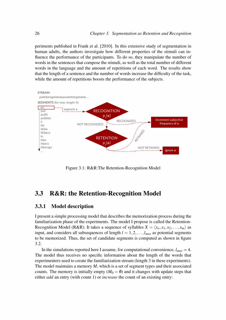
Figure 3.1: R&R:The Retention-Recognition Model
3.3 R&R: the Retention-Recognition Model
3.3.1 Model description
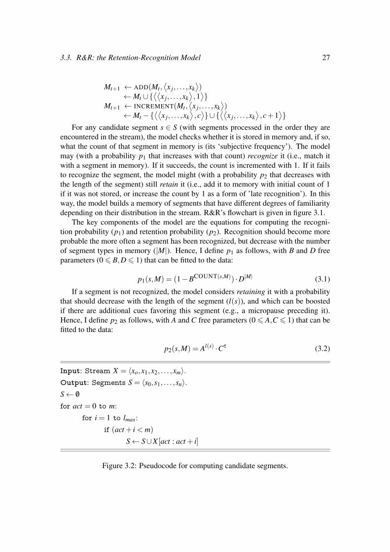
I present a simple processing model that describes the memorization process during thefamiliarization phase of the experiments. The model I propose is called the Retention-Recognition Model (R&R). It takes a sequence of syllables X = 〈xo,x1,x2, . . . ,xm〉 asinput, and considers all subsequences of length l = 1,2, . . . , lmax as potential segmentsto be memorized. Thus, the set of candidate segments is computed as shown in figure3.2.
In the simulations reported here I assume, for computational convenience, lmax = 4.The model thus receives no specific information about the length of the words thatexperimenters used to create the familiarization stream (length 3 in these experiments).The model maintains a memory M, which is a set of segment types and their associatedcounts. The memory is initially empty (M0 = /0) and it changes with update steps thateither add an entry (with count 1) or increase the count of an existing entry:
3.3. R&R: the Retention-Recognition Model 27
Mt+1 ← ADD(Mt ,⟨x j, . . . ,xk
⟩)
←Mt ∪{⟨⟨
x j, . . . ,xk⟩,1⟩}
Mt+1 ← INCREMENT(Mt ,⟨x j, . . . ,xk
⟩)
←Mt−{⟨⟨
x j, . . . ,xk⟩,c⟩}∪{
⟨⟨x j, . . . ,xk
⟩,c+1
⟩}
For any candidate segment s ∈ S (with segments processed in the order they areencountered in the stream), the model checks whether it is stored in memory and, if so,what the count of that segment in memory is (its ‘subjective frequency’). The modelmay (with a probability p1 that increases with that count) recognize it (i.e., match itwith a segment in memory). If it succeeds, the count is incremented with 1. If it failsto recognize the segment, the model might (with a probability p2 that decreases withthe length of the segment) still retain it (i.e., add it to memory with initial count of 1if it was not stored, or increase the count by 1 as a form of ’late recognition’). In thisway, the model builds a memory of segments that have different degrees of familiaritydepending on their distribution in the stream. R&R’s flowchart is given in figure 3.1.
The key components of the model are the equations for computing the recogni-tion probability (p1) and retention probability (p2). Recognition should become moreprobable the more often a segment has been recognized, but decrease with the numberof segment types in memory (|M|). Hence, I define p1 as follows, with B and D freeparameters (0 6 B,D 6 1) that can be fitted to the data:
p1(s,M) = (1−BCOUNT(s,M)) ·D|M| (3.1)
If a segment is not recognized, the model considers retaining it with a probabilitythat should decrease with the length of the segment (l(s)), and which can be boostedif there are additional cues favoring this segment (e.g., a micropause preceding it).Hence, I define p2 as follows, with A and C free parameters (0 6 A,C 6 1) that can befitted to the data:
p2(s,M) = Al(s) ·Cτ (3.2)
Input: Stream X = 〈xo,x1,x2, . . . ,xm〉.Output: Segments S = 〈s0,s1, . . . ,sn〉.S← /0
for act = 0 to m:for i = 1 to lmax:
if (act + i < m)
S← S∪X [act : act + i]
Figure 3.2: Pseudocode for computing candidate segments.

28 Chapter 3. Segmentation as Retention and Recognition
The A parameter thus describes how quickly the retention probability decreaseswith the length of a segment. The factor Cτ attenuates this probability unless an addi-tional cue boosts it; here, I consider only the micropauses from Pena et al. [2002] asadditional cues, and set τ = 0 if there has been such a pause, and τ = 1 if not. Puttingeverything together, the model can be described in pseudocode as in figure 3.3.
Input: Stream X , and empty memory M0← /0.Output: Memory Mn+1./∗ Compute candidate segments: ∗/S← 〈s0,s1, . . . ,sn〉/∗ Process each segment: ∗/for i = 0 to n:
/∗ Compute the recognition probability: ∗/p1 = p1(si,Mi)/∗ Compute the retention probability: ∗/p2 = p2(si,Mi)/∗ Draw two random numbers ∗/r1 ∼U(0,1)r2 ∼U(0,1)/∗ Recognize, retain or ignore: ∗/IF (r1 < p1)
Mi+1← increment(si,Mi)ELSE IF (r2 < p2)
Mi+1← add(si,Mi)ELSE
Mi+1←Mi
Figure 3.3: Pseudocode describing the R&R model.
R&R is thus a simple model, but it gives a surprisingly accurate match with empir-ical data, as I will present in the next sections, without even taken processes such asforgetting, priming, interference and generalization into account.
3.3.2 Qualitative behaviour of the modelR&R exhibits rich-get-richer dynamics: as the subjective frequency of a sequencegrows, the probability for this sequence to be recognized on its next occurrence in thestream also grows, and therefore its subjective frequency is likely to increase again. Asequence, however, cannot be recognized before it has been retained. The stochasticityof the retention will cause some sequences to be retained later than others, so not all

3.3. R&R: the Retention-Recognition Model 29
Parameters R&R Skew Words Skew PartwordsA=0.4 B=0.4 C=0.5 D=0.6 -0.13 2.29A=0.5 B=0.5 C=0.5 D=0.5 0.88 1.41A=0.6 B=0.7 C=0.7 D=0.3 -0.86 -0.37A=0.9 B=0.4 C=0.5 D=0.6 0.68 0.0
Table 3.1: Skew for several parameter settings of R&R.
sequences will benefit equally from a high recognition probability. With this interplaybetween the stochasticity of retention and the (also stochastic) rich-get-richer dynamicsof recognition, even sequences that are identical in terms of absolute frequency mayend up with substantially different subjective frequencies.
This intuition should be reflected in the distribution of subjective frequencies. Firstof all, given the behaviour described above, we expect the frequency distributions tobe skewed, since some sequences should be quickly favoured (and thus end up withhigh subjective frequencies) while others will be picked up later and therefore theywill end up having smaller subjective frequencies. For this same reason, another pre-diction is that words and partwords will show overlapping distributions, that is, wordsand partwords will not be clearly differentiated given their frequencies; instead, somepartwords should have higher frequencies than some words. In short, the R&R modelpredicts (i) a notable degree of skew and (ii) overlapping distributions of words andpartwords.
I explore two different techniques to verify these predictions. In order to test for(i), I apply one metric of skew from the literature on summary statistics, concretelyPearson’s second coefficient of skewness (also known as median skew). As for (ii), Iuse a qualitative approach, based on plotting the subjective frequencies of words andpartwords in the same graph, in order to visualize whether the distributions overlap.
Regarding the first technique — the quantification of the degree of skew —, themedian skew is defined as follows:
3(mean−median)standard deviation
, (3.3)
This coefficient exploits the fact that the mean and the median are separated fromeach other in skewed distributions. So 0 indicates no skew, while greater values indi-cate greater skew, with the direction reflected in the sign.
Table 3.1 shows the median skew of a few parameter settings of the R&R model.As can be seen, the degree of skew varies substantially. This casts doubts on whetherthis summary statistic is a proper choice in this case, since the intuition sketched abovemay not be reflected in the relation between the mean and the median of the data.
As for the qualitative analysis on the distributions of words and partwords, the cor-responding graph can be seen in figure 3.4, which shows the distribution of the subjec-tive frequencies computed by the R&R model for the baseline experiment in Pena et al.[2002], for different parameter settings. As can be observed, the model presents dif-

30 Chapter 3. Segmentation as Retention and Recognition
ferent behaviour under different parameter settings, with most of them yielding over-lapping distributions (a very large value for A is required for the distributions to beseparated).
The qualitative behavior of R&R predicts therefore that the responses of subjectsin the segmentation experiments will exhibit considerable degree of skew, as well asdistributions that overlap. The next section analyzes whether this prediction is foundin the empirical results.
Figure 3.4: Subjective frequencies in four simulations of the R&R model, with differ-ent parameters, when familiarized with the AXC language of Pena et al. [2002]. Greenbars (w) are words and red bars (pw) are partwords.
3.4 Predictions and empirical data
3.4.1 Prediction of observed skew in response distribution in ratsAfter having identified the main predictions of the R&R model, I now investigatewhether the empirical data exhibits signatures of these predictions. In order to studywhether this is the case with the experimental data from rats, I have exposed the modelto the same stimuli used in Toro and Trobalon [2005], which is a stream of syllablesthat I created by following the description of the familiarization stream in Pena et al.[2002]. In that stream, words appear all with exactly the same frequency (e.g. puliki,
3.4. Predictions and empirical data 31
Words PartwordsNo Pauses 1.01 1.07With Pauses 1.02 1.59
Table 3.2: Median skew of the experimental data with rats.
beraga, tafodu, etc. appear 100 times each in the 10 minute condition). Partwords havea much lower frequency (approximately 1/2 of the word frequency)3.
Toro and Trobalon measure how rats respond to the test triples, based on how muchthey press a lever; in this way, they assess the recognition of words, partwords andrulewords. In order to test whether the responses exhibit signatures of skew, I plot thedata (which the authors kindly shared) in figure 3.6. The graph shows, with small solidcircles, the ordered responses of rats after familiarization to the stream without andwith pauses respectively.
What can be observed in such plot is that, in line with the observations made above,R&R generates skewed distributions when presented with this familiarization stream.Such a skew has, to the best of my knowledge, not been reported yet in the analysisof experimental ALL results on adults, which all report averages over responses in aforced choice setting. Nor has it been reported in papers on experiments with prelin-guistic infants and animals, which do measure responses to individual test items but allreport averages over stimulus classes.
To evaluate how well the model can fit this data quantitatively, I make the additionalassumption that the measured response rates are directly proportional to the subjectivefrequencies of the triples in the memories of the rats. I then search for parametersettings that produce the best fit (measured with squared error) to the average rat. I fitparameters B and D, and a value4 that combines A and C, to the data without pauses;I then used the data with pauses solely to differentiate between the contributions of Aand C. The pink lines in the graphs give the prediction of the model with the thus fittedparameters, and demonstrate a surprisingly good fit.
As explained before, I hypothesize that the observed skew in the responses (sum-marized in table 3.2) is explained by a skewed distribution of subjective frequenciesof test items. However, an alternative explanation is that the observed skew is merelydue to variability in the responses. In order to investigate this alternative explanation, Ianalyze how skewed would the responses be if they came from a Gaussian distributioncentered on the empirical mean and scaled with the empirical standard deviation. Fig-ure 3.5 shows a histogram of the cumulative probability for 10.000 samples. As can be
3The exact frequency depends on the randomization process by which words are sampled; in thereported simulations I have assumed that Pena et al. repeatedly play the complete sequence of wordsin randomized order. I also tried other processes consistent with the description they give, and obtainedvery similar results.
4As all considered segments have length 3 and there is no information to differentiate between thecontributions of A and C, I estimate the value of A3C instead. I then assume these values as given, andemploy the corresponding data from the experiment with micropauses to estimate A and C.

32 Chapter 3. Segmentation as Retention and Recognition
seen, the probability of observing the empirical skew (or greater positive skew) is verysmall. Therefore, it seems that the observed skew is not just due to random responsevariability.
3.4.2 Prediction of observed skew in response distribution in hu-mans
I have been able to confirm the prediction of skew in the response distribution of ratsbecause I obtained access to the original data, which consisted of responses per item.But when it comes to humans, I encountered some complications: adults are typicallytested in 2AFC tasks, which do not allow for a study of the distribution of responses forsingle items; as for infants, although the type of responses that are recorded (typically,listening times) would allow to investigate the preference for single items, the reporteddata consists only of averages for classes of sequences, and I could not obtain accessto the original data for any of the reported studies (although see footnote 2).
For these reasons, I have run an experiment with human adults to investigate whetherthe skew of response distributions is consistent with that predicted by R&R. For this, Iused stimuli following the structure proposed in Pena et al. [2002].
Methods
Participants13 participants, master students of the University of Amsterdam, participated in thestudy as part of one of their courses.
StimuliThe stimuli consisted of an 11 minute speech stream of synthetic speech syllables gen-erated with eSpeak. I used two conditions that only differed in the randomization ofthe position of a syllable in a word, and the randomization of the order of appearanceof those words. For one group, the words were: jaduki, jamaki, jataki, lidufo, limafo,litafo, sudube, sumabe, sutabe; for the other, the words were: jabeta, jaduta, jakita,mabefo, madufo, makifo, subeli, suduli, sukili. Each word was presented 100 times,and their order of appearance was random with the constrain that one word cannotfollow another of the same family (i.e., that starts and ends with the same syllable).
The test items consist of the nine words of the familiarization stream and nine part-words, also present in the familiarization stream, consisting of two syllables of oneword and one syllable of the next, or of one syllable of one word and two syllablesof the next. These eighteen items appear two times in the test set, and their order ofappearance is randomized (but constant across participants), with the constraint thatthe same sequence does not appear consecutively.
ProcedureThe participants were randomly assigned to one of the two conditions. The stimuli

3.4. Predictions and empirical data 33
(a) Without pauses.
(b) With pauses.
Figure 3.5: Reversed cumulative probability of the median skew coefficient, for 10.000samples from a Gaussian distribution based on the empirical mean and standard devia-tion of the responses of the rats. The empirical median skew coefficient is marked witha vertical line.

34 Chapter 3. Segmentation as Retention and Recognition
(a) Without pauses.
(b) With pauses.
Figure 3.6: Responses of rats (blue) and subjective frequencies of the model (pink). Windicates words; P indicates partwords; both ordered by response frequency. Parametersetting of the model: A=0.3; B=0.92; C=0.93; D=0.94.
were presented with the use of a web form. They were instructed to listen to the wholefamiliarization stream, for which they would have to answer questions afterwards. Inthe test phase, each test item was presented acoustically, followed with the question‘Is this sequence part of the language you have heard?’, to be answered with yes/no.Afterwards, they were asked to rate their confidence in the previous answer, in a scalefrom 1 to 7 (where 1 is minimum confidence and 7 is maximum).
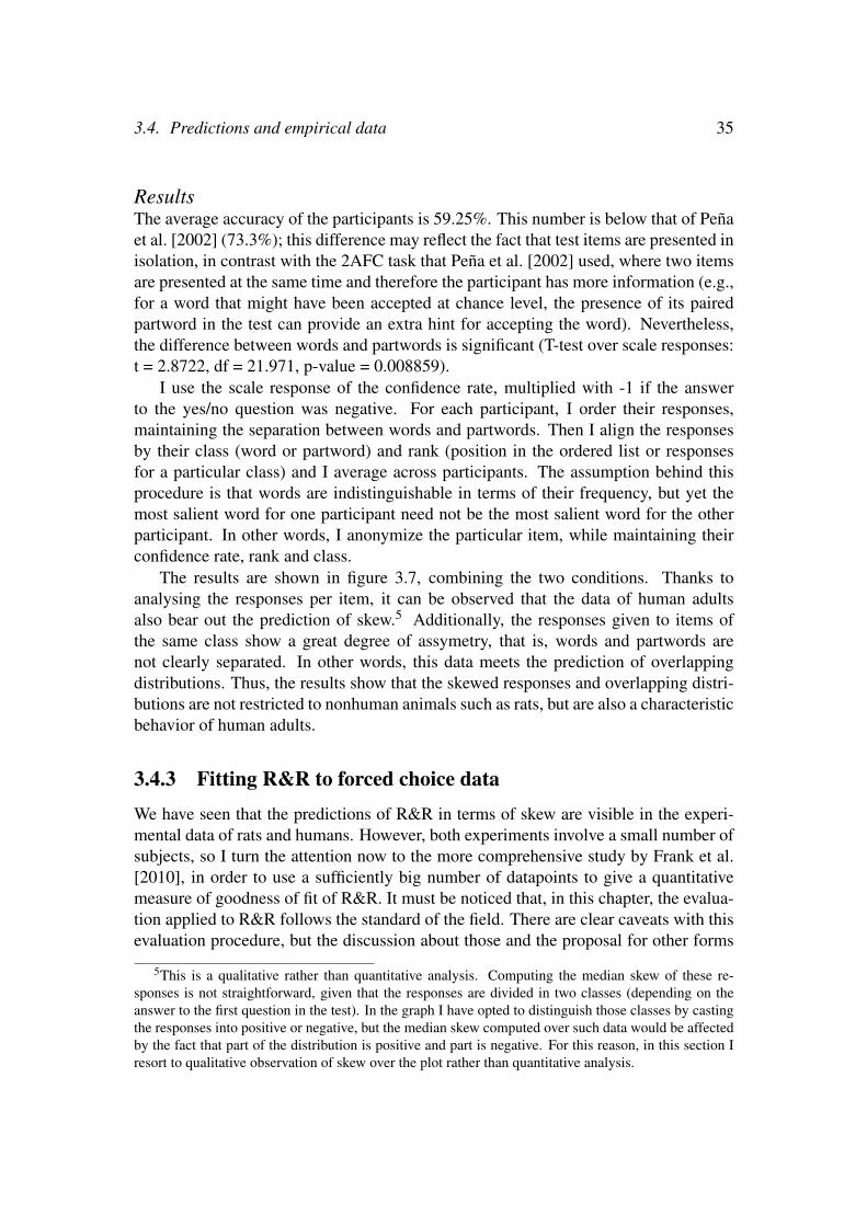
3.4. Predictions and empirical data 35
ResultsThe average accuracy of the participants is 59.25%. This number is below that of Penaet al. [2002] (73.3%); this difference may reflect the fact that test items are presented inisolation, in contrast with the 2AFC task that Pena et al. [2002] used, where two itemsare presented at the same time and therefore the participant has more information (e.g.,for a word that might have been accepted at chance level, the presence of its pairedpartword in the test can provide an extra hint for accepting the word). Nevertheless,the difference between words and partwords is significant (T-test over scale responses:t = 2.8722, df = 21.971, p-value = 0.008859).
I use the scale response of the confidence rate, multiplied with -1 if the answerto the yes/no question was negative. For each participant, I order their responses,maintaining the separation between words and partwords. Then I align the responsesby their class (word or partword) and rank (position in the ordered list or responsesfor a particular class) and I average across participants. The assumption behind thisprocedure is that words are indistinguishable in terms of their frequency, but yet themost salient word for one participant need not be the most salient word for the otherparticipant. In other words, I anonymize the particular item, while maintaining theirconfidence rate, rank and class.
The results are shown in figure 3.7, combining the two conditions. Thanks toanalysing the responses per item, it can be observed that the data of human adultsalso bear out the prediction of skew.5 Additionally, the responses given to items ofthe same class show a great degree of assymetry, that is, words and partwords arenot clearly separated. In other words, this data meets the prediction of overlappingdistributions. Thus, the results show that the skewed responses and overlapping distri-butions are not restricted to nonhuman animals such as rats, but are also a characteristicbehavior of human adults.
3.4.3 Fitting R&R to forced choice dataWe have seen that the predictions of R&R in terms of skew are visible in the experi-mental data of rats and humans. However, both experiments involve a small number ofsubjects, so I turn the attention now to the more comprehensive study by Frank et al.[2010], in order to use a sufficiently big number of datapoints to give a quantitativemeasure of goodness of fit of R&R. It must be noticed that, in this chapter, the evalua-tion applied to R&R follows the standard of the field. There are clear caveats with thisevaluation procedure, but the discussion about those and the proposal for other forms
5This is a qualitative rather than quantitative analysis. Computing the median skew of these re-sponses is not straightforward, given that the responses are divided in two classes (depending on theanswer to the first question in the test). In the graph I have opted to distinguish those classes by castingthe responses into positive or negative, but the median skew computed over such data would be affectedby the fact that part of the distribution is positive and part is negative. For this reason, in this section Iresort to qualitative observation of skew over the plot rather than quantitative analysis.
36 Chapter 3. Segmentation as Retention and Recognition
Figure 3.7: Confidence rates, averaged per ranked item.
of evaluation is left for chapter 4.Frank et al. investigate how distributional aspects of an artificial language have
an effect on the performance of human adults in segmentation. Each of their threeexperiments involves a range of conditions that vary in one particular dimension: (i)sentence length, (ii) amount of exposure (number of tokens) and (iii) vocabulary size(number of word types).
The stimuli consists of an auditory sequence of sentences, each of which is cre-ated from a sample of artificial (unexisting) words. The sentences are separated witha silence gap of 500 ms, while there is no acoustic nor prosodic cue indicating theseparation between words within a sentence. After the participants have been exposedto a sample of sentences thus constructed, they participate in a 2-Alternative-Forced-Choice test (2AFC). The two alternatives in the test consist on one word from theartificial language (a correctly segmented sequence), and one “part-word” (a sequenceresulting from incorrect segmentation).
To analyze the results, the authors average the performance (i.e. the number ofcorrect choices) over participants. These averages are arranged to form a curve thatshows the performance for different values of sentence length, amount of exposureand vocabulary size, as can be seen in the continuous line in figure 3.8. What theresulting curves show is that: (i) human adults have more difficulty in segmentingwords when sentences are longer, presumably because they do not benefit from theextra cue provided by the silence gaps; (ii) when the amount of word tokens is varied,more occurrences of words facilitate the identification of such words, and (iii) the sizeof the vocabulary seems to cause lower performance in the experiment, with an almost-

3.4. Predictions and empirical data 37
linear inverse relation.Given that the stimuli used in this experiment contain longer pauses, the model
needs some small adaptations. The design of R&R was initially inspired by the resultspresented in Pena et al. [2002], where the pauses in the stimuli, when present, have alength of 25ms, and this duration is supposed to be perceived by humans only sublim-inally. The stimuli used in Frank et al. [2010] differ significantly in the use of pauses,which have a duration of 500ms, and are used as a separation of sentences instead ofwords. I adapt the formula for Retention, using an exponential parameter regulatingthe effect of the pauses (Eq. (3.4)): 6
p2(s) = Alength(s)·µ (3.4)
µ =
{µwp after a pauseµnp otherwise
The other adaptation is the use of the Luce Rule [Luce, 1963]. Following Franket al. [2010], I apply the Luce Rule to transform the scores produced by the R&R model(the subjective frequencies) to behavioural predictions for a 2AFC task. Given a pairof sequences s1 and s2 in test, the Luce Rule defines the probability of choosing s1 ascan be seen in Equation 3.5:
P(s1) =Sub jFreq(s1)
Sub jFreq(s1)+Sub jFreq(s2)(3.5)
Once the scores have been transformed to probabilities, the performance of themodels is computed as the mean probability of choosing the correct item, averagedover participants and test trials. These datapoints are arranged in a curve in the sameway as with human participants, and the correlation in the shape of these curves —measured with Pearson’s r— is taken as an indication of good fit.
The three experiments are simulated with R&R, transforming its output (the subjec-tive frequencies) into test trials with the Luce Rule. A search is run over the parameterspace, in order to find which parameters yield best correlation with human perfor-mance7. Clearly, optimizing the parameters on the same data on which the model isevaluated brings the risk of overfitting, but the evaluation is nevertheless carried out inthis way so that the results remain comparable to other model simulations; this com-parison and a discussion on better ways to evaluate are presented in chapter 4. The bestresults of R&R are shown in figure 3.8.
When it comes to experiment 1, one interpretation for the good fit is that R&R ex-plicitly models the effect of the silence gaps. By increasing the length of the sentenceswhile keeping the number of types and tokens constant, the stimuli necessarily con-
6As explained in footnote 4, the contributions of the two parameters A and C cannot bedistinguished,so I opted to change the formula in this way. I keep the value of the new parameter µnp at 1.0 in thissimulation so that the resulting model remains comparable.
7The only parameter that I keep fixed in the search is µnp = 1.0, since the interpretation of the relativeimportance of pauses is clearer if only one of the µ parameter is varied.

38 Chapter 3. Segmentation as Retention and Recognition
0 5 10 15 20 2550
60
70
80
90
100
Perform
ance
r=0.98
Experiment 1
humansR&R: A=0.008 B=0.923 D=0.866 munp=1.000 muwp=0.234
(1) Varying sentence length.
0 200 400 600 800 1000 120050
60
70
80
90
100
Perform
ance
r=0.94
Experiment 2
humansR&R: A=0.008 B=0.923 D=0.866 munp=1.000 muwp=0.234
(2) Varying the number of tokens.
2 3 4 5 6 7 8 9 10 1150
60
70
80
90
100
Perform
ance
r=0.98
Experiment 3
humansR&R: A=0.008 B=0.923 D=0.866 munp=1.000 muwp=0.234
(3) Varying the vocabulary size.
Figure 3.8: Curve of performance for all the different conditions in the experiments inFrank et al. [2010].
sist of fewer sentences; therefore, the number of silence gaps also decreases. For thisreason, the performance of R&R declines with longer sentences, since it cannot obtainthe same benefit from exploiting silence gaps. This explanation can be supported bylooking at the values of the µwp parameter: the best fit of the model requires a lowvalue for this parameter (µwp = 0.234)), so in the presence of a pause it substantiallyboosts the otherwise very small (Aµnp = 0.008) retention probability.
The second experiment was interpreted by Frank et al. as suggesting that humansmay be forgetting much of what they hear, which would explain the increased perfor-mance with the number of tokens. R&R accounts for these results thanks to a prob-abilistic form of retention (combined with recognition that allows for the “correct”segments to be reinforced in memory); thus, the R&R model suggests that forgettingneed not be incorporated in a model of segmentation, at least for the length of thestimuli used in these experiments.
Experiment 3 can be easily interpreted with R&R. The effect of increasing vocab-ulary size only has an effect in the distributional properties of the stream, which result

3.5. Conclusions 39
in less statistically coherent partwords. Still, humans do not seem to exploit this fact;instead, their performance decreases when increasing vocabulary size. Therefore, itseems that humans have some inherent difficulty in recognizing items over a large col-lection of types, possibly due to interference. R&R explicitly models this phenomenonwith a parameter that penalizes recognition based on the number of memorized types.In line with this intuition, the corresponding parameter value for the best fit amounts toD = 0.86, which substantially decreases the chance for successful recognition8. There-fore, in conditions of high number of types, humans have an increased difficulty inrecognizing sequences, most likely originating from the process of matching the inputsegment to one of the many segments stored in memory.
3.5 ConclusionsArtificial Language Learning has proven to be very useful for finding out which cuesare exploited when subjects are learning an unknown language. In this work I focuson one of the first problems that learners face: the identification of words in a speechstream.
With R&R, I provide a theory that considers the process of segmentation as theinteraction of two cognitive mechanisms: retention and recognition. Pitched at theprocessing level, and with a very simple formalization, R&R offers a way to understandthe pattern of experimental results that I find in the literature.
Models do not only help us reason about the cognitive processes underlying ex-isting experiments, but also allow us to make predictions for experimental results.R&R predicts that the memorized segments of the familiarization stream should ex-hibit skewed and overlapping distributions of subjective frequencies; an observationthat, to my knowledge, has never been reported before.
To confirm this prediction, I have revisited the experimental results of Pena et al.[2002], on human adults, and Toro and Trobalon [2005], on rats; focusing on the re-sponses per test item: by replicating the experiment with a different test type in theformer, and by providing a more fine-grained analysis in the latter. I have used quali-tative and quantitative techniques to show that both datasets present skewed and over-lapping distribution of responses, albeit the quantitative metric employed (the medianskew) did not appear to be a very reliable measure for this prediction. Furthermore,R&R is also shown to provide a good quantitative fit to the experimental data on 2AFCresponses of Frank et al. [2010].
I conclude that the R&R model constitutes a simple yet powerful characterizationof the mechanisms underlying speech segmentation that shows an excellent correlationwith the experimental data, and that has already allowed me to provide a new obser-
8Even though the values that parameter D range from 0.0 to 1.0, a value like 0.86 turns out to berelatively small. This is because the model computes D|M|, and the number of types |M| stored by R&Rgrows very rapidly due to the memorization of segments of any length. This entails that the whole termquickly becomes very small, so values of D that are close to 0.0 are impractical.

40 Chapter 3. Segmentation as Retention and Recognition
vation of the existing data, proving therefore to be a promising tool for revealing theproperties of this basic process of language learning.
Chapter 4How should we evaluate models of
segmentation in Artificial Language Learning?
4.1 IntroductionThe previous chapter presented the Retention and Recognition model, a model of seg-mentation in Artificial Language Learning experiments. Using existing methods forevaluating models, I showed that R&R provides a good fit to a range of empirical data.However, other models of segmentation have been proposed before, and they have alsobeen assessed against empirical data. Thus, it is also necessary to also analyze howdoes R&R compare to the existing models.
The goal of this chapter is to address this issue while taking a broader perspective,that is, reflecting on general aspects of evaluation of segmentation models in ALL. AsI stated in § 2.4, it is very important to challenge computational models with evaluationprocedures based on empirical evidence (external validation, [Zuidema and de Boer,2014]), and which are demanding enough to allow us to distinguish between differentproposals.
The structure of this chapter is as follows.1 First, I describe the most relevantmodels of segmentation in Artificial Language Learning, and I relate them to R&R.Second, I review how these models have been evaluated before, distinguishing be-tween evaluation based on internal representations and evaluation over performancein 2-Alternative-Forced-Choice (2AFC) tests. The latter is further illustrated with acomparison of segmentation models, based on an extension of the study by Frank et al.[2010] –which I extend to also incorporate R&R. I reflect on what can be learnt about
1The content in this chapter is based on the following publications:
• Alhama, Scha, and Zuidema [2015] How should we evaluate models of segmentation in artifi-cial language learning? Proceedings of 13th International Conference on Cognitive Modeling.
• Alhama and Zuidema [2017b] Segmentation as Retention and Recognition: the R&R model.Proceedings of the 39th Annual Conference of the Cognitive Science Society.
41

42 Chapter 4. Model evaluation
models when applying this evaluation procedure, and argue that a different type ofevaluation would result in a better understanding of the differences between models. Ithen propose one such procedure for evaluating models, and then conclude the chapterwith a call for different experiments and encouraging data sharing.
4.2 Models of SegmentationThere exist several models of segmentation in the literature; here, I focus on a rep-resentative sample, consisting of the most prominent models at each level of analysis[Marr, 1982].
At Marr’s computational level of analysis we find the Bayesian Lexical Model(BLM henceforth), presented in Goldwater et al. [2006, 2009] and adapted for ALL inFrank et al. [2010]. The BLM conceptualizes the problem of segmentation from theperspective of a Bayesian model: given the input (familiarization) stream, the modelattempts to reconstruct the generative process that generated the stream in the firstplace. As explained in § 2.3.3, this is done by probabilistic inference that searchesthrough a space of possible generative hypotheses. In the case of segmentation, the hy-potheses space consists of the possible segmentations, that is, each hypothesis consistsof the set of words of the language that may have generated the observed stream. Thus,the ‘probability of a word’ refers to the probability of a sequence being a word underthe current hypothesis. This is the reverse perspective from that of the R&R model.R&R is a processing model, and therefore the probabilities of sequences refer to theprobability of retaining or recognizing them while processing the input.
The BLM is driven by rich-get-richer dynamics similar to R&R, implemented asa Dirichlet process. The main assumptions of this process are: (a) the probability ofa word in the ith position is proportional to the number of occurrences of this word inprevious positions; (b) the relative probability for a new word type in the ith position isinversely correlated with the total number of word tokens, and (c) a new word type ismore probable if it is shorter.
How do these principles relate to R&R? Assumption (b) does not allow for directcomparison, since R&R is not a generative model, and therefore it does not providea probability for new types —rather, the incorporation of new types to the memoryof the model depends on the retention probability, and it is based on a preference forshorter sequences (an intuition encoded also in assumption (c) of the Bayesian model).As for assumption (a), the same principle is incorporated in the recognition processin R&R; however, in R&R the counts of the number of occurrences of a word arebased on the subjective frequencies resulting from memorization, while in the BLM,these counts are based on absolute frequencies of the current hypothesis. This reflectsa fundamental difference between the two approaches, which concerns their level ofanalysis [Marr, 1982]. The BLM is framed at Marr’s computational level; therefore,since it does not incorporate any perceptual or memory constraints, it can operate overabsolute frequencies (although some of the extensions in Frank et al. [2010] incorpo-

4.2. Models of Segmentation 43
rate limitations on memory capacity, leading to somewhat hybrid models; I return tothis point later). In contrast, R&R is a processing model, whose dynamics are entirelybased on cognitive processes of retention and recognition, and therefore the frequencycounts are a result of these mechanisms.
At the processing level, the most well known model is PARSER, a symbolic modelthat accounts for segmentation with basic principles of associative learning and chunk-ing. Starting with a few primitives (typically, the syllables of the stream), PARSERincrementally builds a lexicon of segments, each of which is stored with an associatedweight that has an effect on determining which segments are going to be memorizednext. The size of the next segment to be perceived is determined randomly; however,the units that compose this segment will be either primitives or already-memorizedsegments that have a weight higher than a certain threshold. As an example, if thesize of the next segment to be perceived is 2, it might be composed of two primitives(syllables), two segments (larger than the syllables) or one of each. The algorithmchooses the combination that allows the largest units, from left to right. For every newsegment that is perceived, its weight in memory is incremented (or it’s added with aninitial weight), but the smaller units that compose it are decremented; this is meant asa process of interference. Additionally, at each timestep, all the units in memory havetheir weights decreased, as a form of decay.
Both PARSER and R&R are exemplar-based models that build a lexicon of seg-ments (exemplars), and use this lexicon of already-memorized segments to decide onfurther segments to memorize. Each segment in the lexicon is stored together with ascore that determines the impact of this segment in the next steps of the segmentationprocess. Thus, the models are similar in their procedure, but there are notable differ-ences between them. One of them is the probabilistic nature of their components. ForPARSER, the stochasticity is limited to the random selection of the size of the next seg-ment to read from the stream. In contrast, R&R considers all possible subsequences ofthe stream (up to a maximum length), as inspired by research in Data-Oriented Parsingtradition [Scha, 1990], but is inherently probabilistic in its basic processes of retentionand recognition.
There exist other differences in the procedure of these approaches. To begin with,the process of retention in R&R penalizes longest segments, on the basis that theywould require more working memory. However, PARSER implements the oppositeprinciple: whenever several segment candidates are possible, it selects those that arebuilt of the longest units, creating in this way a bias for larger segments. As for theprocess of recognition, it is implicitly implemented in PARSER when it maps the nextsegment to be read against the units in memory. This process involves a binary thresh-old: only units with weight above the threshold can be recognized as components ofthe segment (but those below the threshold are retained). In contrast, the interactionbetween recognition and retention in R&R is based on a graded probabilistic choice.Finally, an important difference between the models is that R&R does not implementany form of forgetting.
On the other extreme, at Marr’s implementational level, some connectionist mod-

44 Chapter 4. Model evaluation
els have been proposed in the past, based on recurrent neural networks [Cleeremansand McClelland, 1991, Servan-Schreiber et al., 1991, Christiansen et al., 1998]. Morerecently, an autoencoder that goes by the name of TRACX has been presented andevaluated on a range of experimental datasets [French et al., 2011, French and Cottrell,2014]. As in all autoencoder networks, TRACX is optimized to learn a representationfor the input data. Thus, the model is trained to reproduce the input in its output layer,and the error produced in the output can be interpreted as the degree of recognition ofthe input.
The model processes the input stream sequentially, maintaining a context window.After successful recognition of a segment, the internal representation learnt by the net-work is used as the context for the next segment to be presented. In this way, contigu-ous segments that are successfully recognized are gradually represented as chunks, andtherefore can be recognized as a unit. This approach shares with R&R the intuition thatwords are consolidated in memory after repeated recognition; however, like PARSER,TRACX is a chunking model, that is, it is oriented at the integration of syllables inorder to build larger fragments. In contrast, in R&R, words emerge in a process thatactually penalizes larger fragments, as a consequence of consolidated memorization ofstatistically salient segments.
4.3 Existing evaluation proceduresComputational models need to be evaluated on some criteria to determine their valid-ity as plausible explanations of the phenomena we aim to account for. In this section Ireview some of the methods of evaluation that have been used for models of segmen-tation in ALL.
4.3.1 Evaluation based on the internal representationsOne way to evaluate the adequacy of a model is by exploring some of the propertiesof the representations that it builds. One example is provided in Perruchet and Vin-ter [1998], for the evaluation applied over PARSER. This model builds a symbolicmemory of the extracted sequences, with a weight that represents the strength of theirmemory trace. In order to assess the quality of this built lexicon, the authors report theamount of familiarization needed to meet each of two possible criteria. The first one,called the loose criterion, is fulfilled when the memory contains all the words in thelanguage with the highest weights, although it may contain also other sequences. Onthe other hand, the strict criterion states that the memory must contain all legal wordswith the highest weights, and if there are other memorized sequences then they mustbe ‘legal’ (subparts or concatenation of words, but not partwords).
The model has been evaluated based on the amount of exposure required for eithercriterion to be reached. For instance, Perruchet and Vinter [1998] show that PARSERmeets both the loose and strict criteria with less exposure than that used for human

4.3. Existing evaluation procedures 45
adults in Saffran et al. [1996b], although it is not clear whether the criteria are still metafter full exposure. In the case of the counterpart study with infants [Saffran et al.,1996b], more exposure than the one that infants had was required for PARSER to meeta ‘looser’ version of the loose criterion (concretely, that one of the two words in thetest set have the higher weights in memory). Thus, a tacit assumption of this form ofevaluation is that successful segmentation corresponds to having a memory in whichthe words have the higher weights.
The advantage of this form of evaluation is that the representations that the modelbuilds are directly taken into account, as opposed to evaluation based on behaviouralresponses. However, for this to be a meaningful evaluation, the criteria used needto be independently motivated, otherwise the evaluation may be biased to favour themodellers’ idiosyncratic choices. Actually, the empirical data reported later in thischapter (§ 4.5, figure 4.1) is at odds with these criteria, suggesting that this form ofevaluation is not as useful as originally thought.
The evaluation procedures reported for TRACX [French et al., 2011] are also basedon learnt representations, but since those are not easily observable in the model (giventhat they are not symbolic), the authors indirectly evaluate the representations based onthe error produced by the model when attempting to recognize the represented items.
The metric (called Proportion Better) computes the difference between the scoresfor words and distractors (partwords or nonwords); in the case of TRACX, the scoresare based on the recognition error of the model. This number is then normalized (seeequation 4.1) and compared to the equivalent calculation for the scores of participantsin the experiment, which may be based, for example, on listening times.
ProportionBetter =score(words)− score(partwords)score(words)+ score(partwords)
(4.1)
This evaluation is applied to segmentation experiments with infants [Saffran et al.,1996a, Aslin et al., 1998, French et al., 2011]. It must be noticed thought that this evalu-ation criterion relies on comparing the recognition error of the model, which is directlycomputed from the internal representations, to behavioural responses. Additionally, byaveraging across test trials and participants, the whole dataset is summarized in onesingle number, and is therefore not very strict.
4.3.2 Evaluation based on behavioural responses
Another form of evaluation is also based on behavioural responses. Most of the exper-imental record on segmentation on adults involves some form of 2AFC test betweentarget sequences (words) and distractors (generally a partword or a nonword). Thiskind of data is more difficult to relate to internal representations (since responses forone stimulus depend on the presentation of the alternative item in the test trial), soin order to fit this data models need to postulate an additional hypothesis –a responsemodel– for linking memorized representations to the behavioral responses.
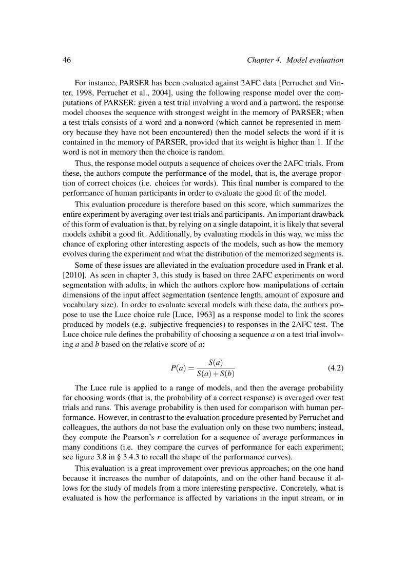
46 Chapter 4. Model evaluation
For instance, PARSER has been evaluated against 2AFC data [Perruchet and Vin-ter, 1998, Perruchet et al., 2004], using the following response model over the com-putations of PARSER: given a test trial involving a word and a partword, the responsemodel chooses the sequence with strongest weight in the memory of PARSER; whena test trials consists of a word and a nonword (which cannot be represented in mem-ory because they have not been encountered) then the model selects the word if it iscontained in the memory of PARSER, provided that its weight is higher than 1. If theword is not in memory then the choice is random.
Thus, the response model outputs a sequence of choices over the 2AFC trials. Fromthese, the authors compute the performance of the model, that is, the average propor-tion of correct choices (i.e. choices for words). This final number is compared to theperformance of human participants in order to evaluate the good fit of the model.
This evaluation procedure is therefore based on this score, which summarizes theentire experiment by averaging over test trials and participants. An important drawbackof this form of evaluation is that, by relying on a single datapoint, it is likely that severalmodels exhibit a good fit. Additionally, by evaluating models in this way, we miss thechance of exploring other interesting aspects of the models, such as how the memoryevolves during the experiment and what the distribution of the memorized segments is.
Some of these issues are alleviated in the evaluation procedure used in Frank et al.[2010]. As seen in chapter 3, this study is based on three 2AFC experiments on wordsegmentation with adults, in which the authors explore how manipulations of certaindimensions of the input affect segmentation (sentence length, amount of exposure andvocabulary size). In order to evaluate several models with these data, the authors pro-pose to use the Luce choice rule [Luce, 1963] as a response model to link the scoresproduced by models (e.g. subjective frequencies) to responses in the 2AFC test. TheLuce choice rule defines the probability of choosing a sequence a on a test trial involv-ing a and b based on the relative score of a:
P(a) =S(a)
S(a)+S(b)(4.2)
The Luce rule is applied to a range of models, and then the average probabilityfor choosing words (that is, the probability of a correct response) is averaged over testtrials and runs. This average probability is then used for comparison with human per-formance. However, in contrast to the evaluation procedure presented by Perruchet andcolleagues, the authors do not base the evaluation only on these two numbers; instead,they compute the Pearson’s r correlation for a sequence of average performances inmany conditions (i.e. they compare the curves of performance for each experiment;see figure 3.8 in § 3.4.3 to recall the shape of the performance curves).
This evaluation is a great improvement over previous approaches; on the one handbecause it increases the number of datapoints, and on the other hand because it al-lows for the study of models from a more interesting perspective. Concretely, what isevaluated is how the performance is affected by variations in the input stream, or in

4.4. Comparing alternative models against empirical data 47
other words, whether increasing or decreasing the difficulty of the segmentation task(based on sentence length, exposure and vocabulary) has a similar effect on modelsand humans. In the next section I discuss this form of evaluation from the perspectiveof model selection.
4.4 Comparing alternative models against empirical dataI have discussed different forms of evaluation in the context of fitting models to empir-ical data. In this section, I argue that even the most adequate of the criteria discussedabove can fall short when it comes to model selection. To do so, I extend the modelcomparison study in Frank et al. [2010] to include also the R&R model. The mod-els simulated by Frank and colleagues include the ones previously described (BLMand PARSER, with the latter addition of TRACX, reported in French et al. [2011]),and four additional approaches: Transitional Probabilities (TP), a Bayesian version ofTransitional Probabilities (Bayesian TPs), Mutual Information (MI), and a version ofMI model that segments sequences that exceed a threshold both on MI and raw fre-quency counts (MI Clustering, Swingley [2005]). Due to their simplicity, these modelsare not reviewed in this chapter; it suffices to say that they all share the property ofbeing normative models over bigrams.
Table 4.1 summarizes the goodness of fit between the models and the experimentaldata, based on Pearson’s r correlation, as described before. As can be seen, for theparameter setting that yields better fit in the three experiments (A = 0.008, B = 0.923,D = 0.866, µnp = 1.0, µwp = 0.234), the R&R model outperforms all the other models.In the previous chapter I reflected on the reasons why R&R provides a good fit to theexperimental data. I now revisit and broaden that discussion to relate the outcome ofR&R to that of other models.
When it comes to experiment 1, the reason for R&R outperforming other modelsmay be that it incorporates an explicit effect of processing the pauses in the stream;concretely, in boosting the retention probability. Since the stimuli contain less pauseswhen sentences are longer, R&R sees its performance decreased, at a similar pace ashumans. It must be noticed though that TRACX also exhibits an excellent correla-tion with the data, as well as two of the versions of the Bayesian Lexical Model (theoriginal, and the one that implements uniform forgetting over types).
In the second experiment, normative models based on point estimates (those basedon TP and MI) do not offer a good fit with the data, since those metrics do not benefitfrom the accumulation of evidence offered by the increased number of tokens (contraryto humans). Frank et al. suggest that humans may be forgetting much of what they hear,which would explain the increased performance with the number of tokens. However,the extended versions of the BLM that incorporate some form of evidence limitation(with input data restricted to a random 4% sample) or forgetting exhibit mixed results(rows 8, 9, 10, 11 on table 4.1), although the results reveal that uniform forgettingover types offers a better correlation. Still, these extensions appear unrealistic from

48 Chapter 4. Model evaluation
Exp. 1: Exp. 2: Exp. 3:Sentence Length #Tokens #Types Mean
1 Transitional Probabilities 0.84 0.43 -0.99 0.092 Mutual Information 0.83 -0.32 -0.99 -0.163 MI Clustering 0.11 -0.81 0.29 -0.134 PARSER 0.00 0.86 0.00 0.285 TRACX 0.92 — 0.97 —∗
6 BLM 0.94 0.89 -0.98 0.28Bayesian TPs
7 4% data 0.82 0.92 0.96 0.90BLM
8 4% data 0.88 0.85 0.90 0.87BLM
9 Uniform forgetting (types) 0.95 0.92 0.73 0.86BLM
10 Prop. forgetting (types) 0.88 0.87 0.88 0.87BLM
11 Uniform forgetting (tokens) 0.86 0.82 0.97 0.8812 R&R 0.98 0.94 0.98 0.97
Table 4.1: Comparison of model results to human performance. The reported metricis Pearson’s r. Experiment 1 is based on varying sentence length; experiment 2 onvarying the number of word tokens, and experiment 3 on varying the number of wordtypes. ∗Experiment 2 was not reported in French et al. [2011]. Therefore, the meancan be taken to be 0.63 (for a Pearson’s r of 0.0 in experiment 2) or 0.945 (averagingonly over experiments 1 and 3).

4.5. A proposal: evaluation over response distributions 49
a cognitive perspective (e.g. forgetting a randomly drawn type when memory capac-ity is full), and additionally, the resulting models are somewhat difficult to interpret,since after incorporating memory limitations, they are different from computationallevel approaches. PARSER offers a more intuitive account of forgetting, with modestcorrelation with human data; however, this model has zero correlation in the other ex-periments. On the other hand, the rich-get-richer form of recognition combined witha process of retention as defined in R&R yields a better correlation than a process ofrecognition with forgetting.
Also on experiment 3, the R&R model exhibits the best correlation with humandata, followed closely by TRACX and the Bayesian Lexical Model with uniform for-getting of tokens. Again, normative models show the opposite trend from humans(rows 1, 2, 3, 6 on table 4.1), since they do not have any memory limitations, and thusthe effect of increasing vocabulary size only has an effect on the distributional proper-ties of the stream, which result in less statistically coherent partwords. Thus, the sameissues about forgetting discussed above apply to this experiment. However, with theexception of TRACX and R&R, the models that perform better in experiment 2 are notthe ones that excel in experiment 3; actually, results on the BLM model suggest thatuniform forgetting of tokens and 4% limitation on the input are better accounts of for-getting. Note that, as explained before, TRACX and R&R do not implement forgetting;actually, R&R explains these results based on the assumption that recognition over alarge number of types is necessarily more difficult, and does so by explicitly incorpo-rating a parameter (D) that penalizes recognition based on the number of memorizedtypes.
But in spite of the good performance of R&R, the most relevant issue is that othermodels that are different also offer a good correlation under this evaluation –althoughnever in all the experiments at the same time. Thus, we need another type of evaluationthat allows for finer distinction between models.
4.5 A proposal: evaluation over response distributionsWe have seen that even with the most thorough evaluation procedure that I am aware of,it is not easy to distinguish between different model proposals. On the one hand, evalu-ation procedures based on internal representations could be potentially useful to revealinteresting properties of the models, but it is difficult for modellers to find externalevidence that is informative about the distributional properties of mental representa-tions, since most of the results that could shed some light on this issue are reported asaggregated responses over participants and stimuli classes. On the other hand, modelevaluation based on 2AFC responses do not allow to identify the strength of internalrepresentations, since the observed responses for one sequence are influenced by thepresence of the other sequence in the trial (e.g. an unrecognized word may be chosenbecause the alternative sequence may appear very unfamiliar to the subject).
I argue that, in order to evaluate and compare models, we need at least (i) exper-

50 Chapter 4. Model evaluation
Figure 4.1: Average confidence rates for each test stimulus type, in decreasing order.Confidence rates for negative answers have negative values. (Repeated from chapter 3,Fig. 3.7, for convenience.)
imental data based on (non-binary) responses to individual stimulus (ii) a big enoughnumber of datapoints to fit; additionally, I suggest (iii) to aggregate the responses forindividual test items anonymously. I now elaborate on these points.
There already exist experimental paradigms that are suitable for (i), such as lis-tening times and likert scales. However, these existing paradigms are not frequentlyused for ALL studies on human adults. And although listening times are very oftenthe type of experiment employed for infants, the results reported in papers are gener-ally averages over all participants and class of test items (e.g. mean listening times forwords and nonwords [Saffran et al., 1996a]). Therefore, even though fitting a model toa single quantity is a too lenient criterion, it is often the only alternative that modellerscan resort to. For this reason, in order to meet (ii), modellers need access to morefine-grained data, either in the form of raw responses (which unfortunately are rarelyshared in public repositories2), or a different summarization of the reported data.
Related to the latter, I explore with (iii) an additional way of analyzing data, whichI already advanced in § 3.4.2 (but for convenience I remind of the most relevant de-tails here). Recall that, in such experiment, I replicated the familiarization phase ofexperiment 1 in Pena et al. [2002]; that is, human adult participants are exposed to aspeech stream constructed with words that follow an AiXCi pattern. But, unlike theoriginal experiment, the test phase in this experiment did not consist of a 2AFC ques-
2Although see the github repository of the Language and Cognition lab in Stanford for an exampleof good practice on sharing raw responses: https://github.com/langcog.

4.6. Conclusions 51
tionnaire; instead, each test item (word or partword) is presented in isolation, followedby two questions: first, “Is this sequence a word of the language you have heard?”,which could only be responded with a yes/no answer, and second, “How confident areyou?”, which had to be answered in a likert scale that ranged from 1 (not confident) to7 (very confident). With this type of test I can now explore how much each sequenceis recognized in isolation, meeting requirement (i).
I ran two conditions of this experiment, differing only in the randomization of thewords. Since I found no effect on the different conditions, I plot an aggregate of theresponses, as can be seen in figure 4.1.
This graph is constructed as follows. First, for each subject and for each class oftest item (words and partwords), I order the responses according to their magnitude.Second, I compute the mean response per each anonymous test item; that is, instead ofaveraging for each test stimulus (e.g. averaging the responses for sequence ‘kidada’), Iaverage over responses to stimuli that occupy the same position on ordered responses.In this way, the preferred word for a participant is averaged together with the preferredword of other participants, and the same goes for second preferred, and so on. Third, Icombine information from each class (words and partwords) by ordering the sequencesbased on their score while maintaining class of items identifiable (in this case it isreflected in the colour). Thus, this procedure offers an additional way to analyze datathat allows monitoring effects that are not due to phonetic aspects of a stimulus, but dueto stochasticity and self-reinforcement in processing. This is the type of summarizationthat I suggest in (iii), and it also addresses (ii) in reporting a complete distribution overtest items rather than a final average for each class of stimuli.
Hence, this experiment meets all the points suggested. As shown before, conduct-ing this experiment allowed to confirm the prediction of skew from R&R, an obser-vation that would not have been possible otherwise. It must be noticed that this kindoutput is not expected from every model; for instance, I run the same analysis withPARSER and, as can be seen in figure 4.2, the distribution yielded by the model doesnot feature the same kind of skew: the weights for the partwords are fairly similar; ad-ditionally, words and partwords are clearly separated, rather than having overlappingdistributions as in the human responses. Thus, returning to the question raised beforeabout the effect of implementing forgetting or imperfect storage, it seems that forget-ting in PARSER augments the difference between words and partwords to the extentthat they become clearly separated, unlike in the human responses. In contrast, theimperfect storage provided by R&R yields a distribution of items that is closer to thatobserved in humans.
4.6 ConclusionsComputational models endow us with a very powerful methodology for implementingand simulating an unconstrained number of ideas that describe how cognitive mecha-nisms may be operating. We therefore require strict and informative evaluation proce-
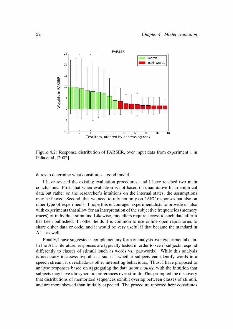
52 Chapter 4. Model evaluation
Figure 4.2: Response distribution of PARSER, over input data from experiment 1 inPena et al. [2002].
dures to determine what constitutes a good model.
I have revised the existing evaluation procedures, and I have reached two mainconclusions. First, that when evaluation is not based on quantitative fit to empiricaldata but rather on the researcher’s intuitions on the internal states, the assumptionsmay be flawed. Second, that we need to rely not only on 2AFC responses but also onother type of experiments. I hope this encourages experimentalists to provide us alsowith experiments that allow for an interpretation of the subjective frequencies (memorytraces) of individual stimulus. Likewise, modellers require access to such data after ithas been published. In other fields it is common to use online open repositories toshare either data or code, and it would be very useful if that became the standard inALL as well.
Finally, I have suggested a complementary form of analysis over experimental data.In the ALL literature, responses are typically tested in order to see if subjects responddifferently to classes of stimuli (such as words vs. partwords). While this analysisis necessary to assess hypotheses such as whether subjects can identify words in aspeech stream, it overshadows other interesting behaviours. Thus, I have proposed toanalyse responses based on aggregating the data anonymously, with the intuition thatsubjects may have idiosyncratic preferences over stimuli. This prompted the discoverythat distributions of memorized sequences exhibit overlap between classes of stimuli,and are more skewed than initially expected. The procedure reported here constitutes

4.6. Conclusions 53
one proposal that has already shown to be useful to show that the process of segmen-tation exhibits some form of self-reinforcement (rich-get-richer) dynamics, but othermethods should be explored in order to challenge computational models with strictevaluation criteria.


Part II
Propensity to Generalize
55

Chapter 5Modelling the Propensity to Generalize
In the previous chapters I have proposed a model for segmentation in ALL, which Ihave contrasted with other existing models. But segmentation is not the only task thatlanguage learners need to master; as advanced in § 1.2, it is useful to conceptualize(some of) the mechanisms involved in language learning as a three-step approach thatstarts with segmentation and culminates in generalization to unseen productions. Inthis chapter, I motivate the need for accounting for the second step: the propensity togeneralize.
5.1 IntroductionFirst of all, let’s recapitulate on the main findings in the field. In the last 20 years, ALLexperiments have become increasingly popular for the study of the basic mechanismsthat operate when subjects are exposed to language-like stimuli. Thanks to these exper-iments, we know that 8 month old infants can segment a speech stream by extractingstatistical information of the input, such as the transitional probabilities between ad-jacent syllables [Saffran et al., 1996a, Aslin et al., 1998]. This ability also seems tobe present in human adults Saffran et al. [1996b], and to some extent in nonhumananimals like cotton-top tamarins [Hauser et al., 2001] and rats [Toro and Trobalon,2005].
Even though this statistical mechanism is well attested for segmentation, it hasbeen claimed that it does not suffice for generalization to novel stimuli or rule learn-ing1. Ignited by a study by Marcus et al. [1999], which postulated the existence ofan additional rule-based mechanism for generalization, a vigorous debate emergedaround the question of whether the evidence from ALL-experiments supports the ex-istence of a specialized mechanism for generalization [Pena et al., 2002, Onnis et al.,2005, Endress and Bonatti, 2007, Frost and Monaghan, 2016, Endress and Bonatti,
1I prefer the term ‘generalization’ because ‘rule-learning’ can be confused with a particular theoryof generalization that claims that the mental structures used in the generalization process have the formof algebraic rules.
57

58 Chapter 5. Modelling the Propensity to Generalize
2016], echoing earlier debates about the supposed dichotomy between rules and statis-tics [Chomsky, 1957, McClelland and Elman, 1986, Pinker and Prince, 1988, Pereira,2000].
In this chapter2 I argue that the dichotomy between rules and statistics is unhelpful;as an alternative, I propose a different conceptualization of the steps involved in gener-alization in ALL. In the following sections, I will first review some of the experimentaldata that has been interpreted as evidence for an additional generalization mechanism[Pena et al., 2002, Endress and Bonatti, 2007, Frost and Monaghan, 2016]. I then re-frame the interpretation of those results with the three-step approach, a proposal ofthe main steps that are required for generalization, involving: (i) memorization of seg-ments of the input, (ii) computation of the probability for unseen sequences, and (iii)distribution of this probability among particular unseen sequences. I model the firststep with the Retention&Recognition model. I propose that a rational characterizationof the second step can be accomplished with the use of smoothing techniques (whichI further demonstrate with the use of the Simple Good-Turing method, [Good, 1953,Gale and Sampson, 1995]. I then argue that the modelling results shown in these twosteps already account for the key aspects of the experimental data; and importantly, itremoves the need to postulate an additional, separate generalization mechanism.
5.2 Experimental RecordSome of the experiments that I review here have been explained before in previouschapters of this dissertation. I nevertheless report all the details that are relevant to thischapter –in spite of the overlap–, for convenience to the reader.
Pena et al. [2002] conduct a series of Artificial Language Learning experimentsin which French-speaking adults are familiarized to a synthesized speech stream con-sisting of a sequence of artificial words. Each of these words contains three syllablesAiXCi such that the Ai syllable always co-occurs with the Ci syllable (as indicated bythe subindex i). This forms a consistent pattern (a “rule”) consisting in a non-adjacentdependency between Ai and Ci, with a middle syllable X that varies. The order of thewords in the stream is randomized, with the constraint that words do not appear con-secutively if they either: (i) belong to the same “family” (i.e., they have the same Aiand Ci syllables), or (ii) they have the same middle syllable X .
After the familiarization phase, the participants respond a two-alternative forced
2The work presented in this chapter was presented before in the following paper:
• Alhama, Scha, and Zuidema [2014] Rule Learning in humans and animals. Proceedings of theInternational Conference on the Evolution of Language.
• Alhama and Zuidema [2016] Generalization in Artificial Language Learning: Modelling thePropensity to Generalize. Proceedings of the 7th Workshop on Cognitive Aspects of Computa-tional Language Learning, Association for Computational Linguistics, 2016, 64-72.
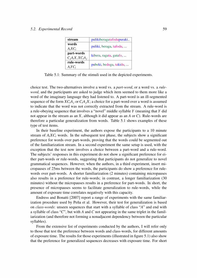
5.2. Experimental Record 59
stream pulikiberagatafodupuraki..wordsAiXCi
puliki, beraga, tafodu, ...
part-wordsC jAiX ,XCiA j
kibera, ragata, gatafo, ...
rule-wordsAiYCi
pubeki, beduga, takidu, ...
Table 5.1: Summary of the stimuli used in the depicted experiments.
choice test. The two-alternatives involve a word vs. a part-word, or a word vs. a rule-word, and the participants are asked to judge which item seemed to them more like aword of the imaginary language they had listened to. A part-word is an ill-segmentedsequence of the form XCiA j or CiA jX ; a choice for a part-word over a word is assumedto indicate that the word was not correctly extracted from the stream. A rule-word isa rule-obeying sequence that involves a “novel” middle syllable Y (meaning that Y didnot appear in the stream as an X , although it did appear as an A or C). Rule-words aretherefore a particular generalization from words. Table 5.1 shows examples of thesetype of test items.
In their baseline experiment, the authors expose the participants to a 10 minutestream of AiXCi words. In the subsequent test phase, the subjects show a significantpreference for words over part-words, proving that the words could be segmented outof the familiarization stream. In a second experiment the same setup is used, with theexception that the test now involves a choice between a part-word and a rule-word.The subjects’ responses in this experiment do not show a significant preference for ei-ther part-words or rule-words, suggesting that participants do not generalize to novelgrammatical sequences. However, when the authors, in a third experiment, insert mi-cropauses of 25ms between the words, the participants do show a preference for rule-words over part-words. A shorter familiarization (2 minutes) containing micropausesalso results in a preference for rule-words; in contrast, a longer familiarization (30minutes) without the micropauses results in a preference for part-words. In short, thepresence of micropauses seems to facilitate generalization to rule-words, while theamount of exposure time correlates negatively with this capacity.
Endress and Bonatti [2007] report a range of experiments with the same familiar-ization procedure used by Pena et al. However, their test for generalization is basedon class-words: unseen sequences that start with a syllable of class “A” and end witha syllable of class “C”, but with A and C not appearing in the same triplet in the famil-iarization (and therefore not forming a nonadjacent dependency between the particularsyllables).
From the extensive list of experiments conducted by the authors, I will refer onlyto those that test the preference between words and class-words, for different amountsof exposure time. The results for those experiments (illustrated in figure 5.1) also showthat the preference for generalized sequences decreases with exposure time. For short
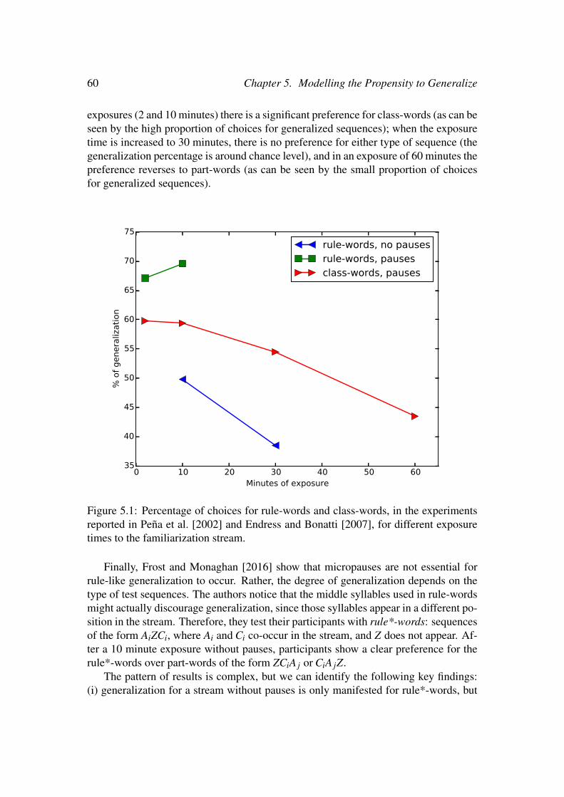
60 Chapter 5. Modelling the Propensity to Generalize
exposures (2 and 10 minutes) there is a significant preference for class-words (as can beseen by the high proportion of choices for generalized sequences); when the exposuretime is increased to 30 minutes, there is no preference for either type of sequence (thegeneralization percentage is around chance level), and in an exposure of 60 minutes thepreference reverses to part-words (as can be seen by the small proportion of choicesfor generalized sequences).
0 10 20 30 40 50 60Minutes of exposure
35
40
45
50
55
60
65
70
75
% o
f gen
eral
izatio
n
rule-words, no pausesrule-words, pausesclass-words, pauses
Figure 5.1: Percentage of choices for rule-words and class-words, in the experimentsreported in Pena et al. [2002] and Endress and Bonatti [2007], for different exposuretimes to the familiarization stream.
Finally, Frost and Monaghan [2016] show that micropauses are not essential forrule-like generalization to occur. Rather, the degree of generalization depends on thetype of test sequences. The authors notice that the middle syllables used in rule-wordsmight actually discourage generalization, since those syllables appear in a different po-sition in the stream. Therefore, they test their participants with rule*-words: sequencesof the form AiZCi, where Ai and Ci co-occur in the stream, and Z does not appear. Af-ter a 10 minute exposure without pauses, participants show a clear preference for therule*-words over part-words of the form ZCiA j or CiA jZ.
The pattern of results is complex, but we can identify the following key findings:(i) generalization for a stream without pauses is only manifested for rule*-words, but

5.3. Understanding the generalization mechanism: a three-step approach 61
not for rule-words or class-words; (ii) the preference for rule-words and class-words isboosted if micropauses are present; (iii) increasing the amount of exposure time cor-relates negatively with generalization to rule-words and class-words (with differencesdepending on the type of generalization and the presence of micropauses, as can beseen in figure 5.1). This last phenomenon, which I call the time effect, is precisely theaspect I want to explain in this work. (Note, in figure 5.1, that in the case of rule-wordsand pauses, the amount of generalization increases a tiny bit with exposure time, con-trary to the time effect. I could not test whether this is a significant difference, forlack of access to the data. Endress&Bonatti, however, provided convincing statisticalanalysis supporting a significant inverse correlation between exposure time and gener-alization to class-words).
5.3 Understanding the generalization mechanism:a three-step approach
Pena et al. interpret their findings as support for the theory that there are at least twomechanisms, which get activated in the human brain based on different cues in theinput. Endress and Bonatti adopt that conclusion (and name it the More-than-One-Mechanism hypothesis, or MoM), and moreover claim that this additional mechanismcannot be based on statistical computations. The authors predict that statistical learningwould benefit from increasing the amount of exposure:
“If participants compute the generalizations by a single associationistmechanism, then they should benefit from an increase in exposure, be-cause longer experience should strengthen the representations built by as-sociative learning (whatever these representations may be).” [Endress andBonatti, 2007]
I think this argument is based on a wrong premise: stronger representations do notnecessarily entail greater generalization. On the contrary, I argue that even very basicmodels of statistical smoothing make the opposite prediction. To demonstrate this in amodel that can be compared to empirical data, I propose to think about the process ofgeneralization in ALL as involving the following steps (illustrated also in figure 5.2):
(i) Memorization: Build up a memory store of segments with frequency informa-tion (i.e., compute subjective frequencies).
(ii) Quantification of the propensity to generalize: Depending on the frequencyinformation from (i), decide how likely are other unseen types.
(iii) Distribution of probability over possible generalizations: Distribute the prob-ability for unseen types computed in (ii), assigning a probability to each gener-alized sequence.

62 Chapter 5. Modelling the Propensity to Generalize
Figure 5.2: Three step approach to generalization: (1) memorization of segments, (2)compute probability of new items, and (3) distribute probability between possible newitems.
Crucially, I believe that step (ii) has been neglected in ALL models of general-ization. This step accounts for the fact that generalization is not only based on theparticular structure underlying the stimuli, but also depends on the statistical proper-ties of the input.
At this point, we can already call into question the MoM hypothesis: as statedin this hypothesis, more exposure time does entail better representation of the stimuli(as would be reflected in step (i)); however, contrary to what is stated in the MoMhypothesis, the impact of exposure time on generalization depends on the model usedfor step (ii). Next, I show that a cognitive model of step (i) and a rational statisticalmodel of step (ii) already account for the time effect.
5.4 Memorization of segments
For step (i) we could choose a segmentation model from the range of models thatreviewed in § 4.2, but since R&R was the most favoured in the analysis, I opt forapplying it in these simulations.
Among the properties of R&R, one that is particularly relevant for this study is theskew that can be observed in the subjective frequencies computed by the model (see§ 3.3.2). This feature is in consonance with the empirical data. Here, I show that thisproperty can also be validated in a different way: when R&R is part of a pipeline ofmodels (like the three-step approach), the skew turns out to be a necessary property forthe success of the next model in the sequence. I come back to this point in section 5.6.
I analyze the effect of the different conditions (exposure time and presence ofpauses) in the memorization of segments computed with R&R. Figure 5.3 shows thepresence of test items (the nine words and nine possible part-words) in the memory of
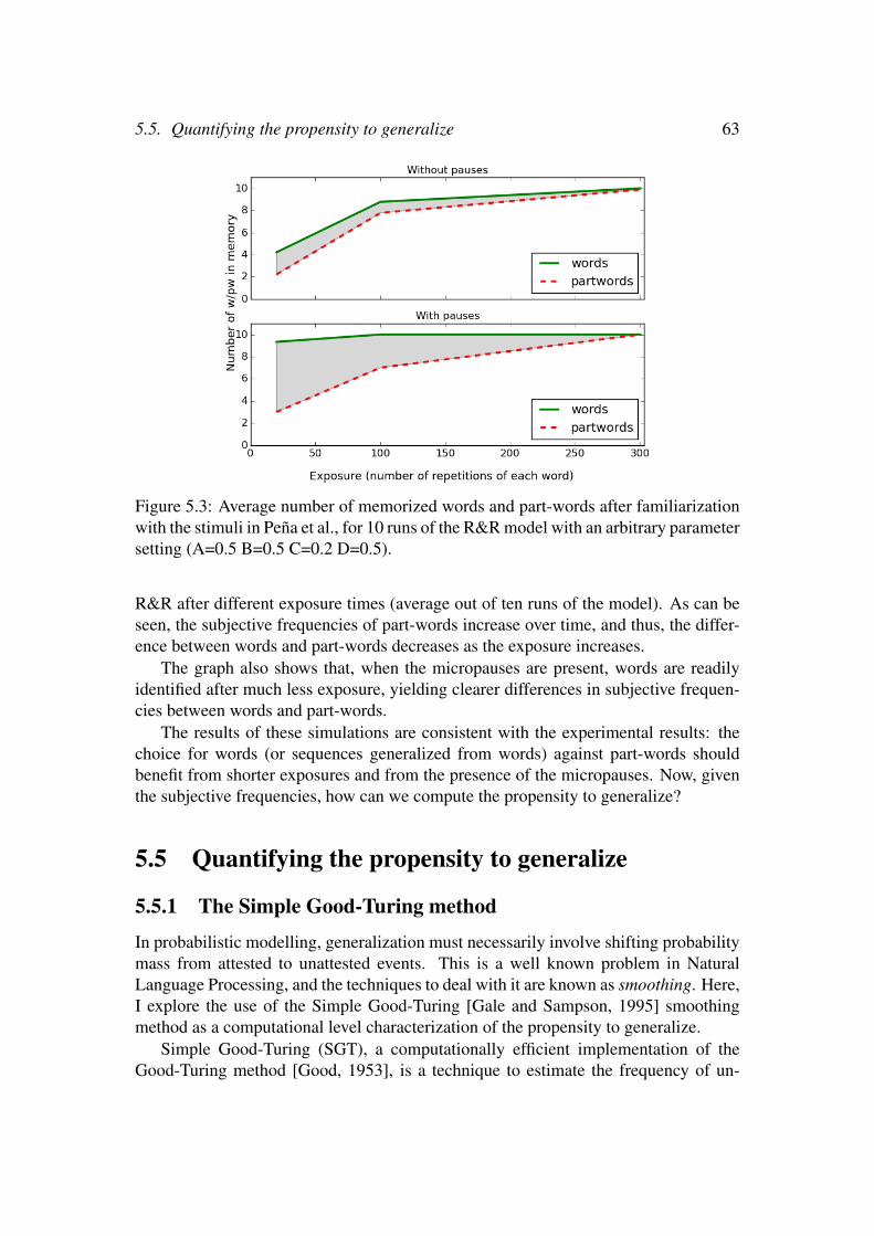
5.5. Quantifying the propensity to generalize 63
Figure 5.3: Average number of memorized words and part-words after familiarizationwith the stimuli in Pena et al., for 10 runs of the R&R model with an arbitrary parametersetting (A=0.5 B=0.5 C=0.2 D=0.5).
R&R after different exposure times (average out of ten runs of the model). As can beseen, the subjective frequencies of part-words increase over time, and thus, the differ-ence between words and part-words decreases as the exposure increases.
The graph also shows that, when the micropauses are present, words are readilyidentified after much less exposure, yielding clearer differences in subjective frequen-cies between words and part-words.
The results of these simulations are consistent with the experimental results: thechoice for words (or sequences generalized from words) against part-words shouldbenefit from shorter exposures and from the presence of the micropauses. Now, giventhe subjective frequencies, how can we compute the propensity to generalize?
5.5 Quantifying the propensity to generalize
5.5.1 The Simple Good-Turing method
In probabilistic modelling, generalization must necessarily involve shifting probabilitymass from attested to unattested events. This is a well known problem in NaturalLanguage Processing, and the techniques to deal with it are known as smoothing. Here,I explore the use of the Simple Good-Turing [Gale and Sampson, 1995] smoothingmethod as a computational level characterization of the propensity to generalize.
Simple Good-Turing (SGT), a computationally efficient implementation of theGood-Turing method [Good, 1953], is a technique to estimate the frequency of un-

64 Chapter 5. Modelling the Propensity to Generalize
seen types, based on the frequency of already observed types. The intuition behindthis method is as follows. Imagine that a biologist goes to the forest, notebook inhand, to write down the number of animals of different species that she encounters(e.g. 20 snails, 10 sparrows, 2 squirrels and 1 snake). This data is a random sample ofthe animal population in the forest, and we use these frequency counts to estimate theprobability that the next animal to be found belongs to one of these species (e.g. thechance that the next animal is a sparrow would be 10/33 = 0.4). However, under thisprobabilistic method, the probability of observing a previously unseen animal (e.g. arabbit) would be zero (0/33 = 0). What Good —acknowledging inspiration from un-published work by Alan Turing— argues is that this is not a good estimation; instead,we should shift some probability mass from the distribution of seen species to estimatethe probability of witnessing an animal belonging to an unseen species.
In order to provide a good estimation for unseen events, Good (and Turing) proposethe following method: first, we take the subjective frequencies r computed by R&Rand, for each of them, we compute the frequency of that frequency (Nr), that is, thenumber of sequences that have a certain subjective frequency r. The values Nr are thensmoothed, that is re-estimated with a continuous downward-sloping line in log space.The smoothed values S(Nr) are used to reestimate the frequencies according to (5.1):
r∗ = (r+1)S(Nr+1)
S(Nr)(5.1)
The probabilities for frequency classes are then computed based on these reesti-mated frequencies:
pr =r∗
N(5.2)
where N is the total of the unnormalized estimates3 .Finally, the probability for unseen events is computed based on the (estimated) 4
probability of types of frequency one, with the following equation:
P0 =S(N1)
N(5.3)
This probability P0 corresponds to what I have called “propensity to generalize”.As can be deduced from the equations, SGT is designed to ensure that the proba-
bility for unseen types is similar to the probability of types with frequency one. Thepropensity to generalize is therefore greater for distributions where most of the prob-
3It should be noted that the reestimated probabilities need to be renormalized to sum up to 1, bymultiplying with the estimated total probability of seen types 1−P0 and dividing by the sum of unnor-malized probabilites.
4SGT incorporates a rule for switching between Nr and S(Nr) such that smoothed values S(Nr) areonly used when they yield significantly different results from Nr (when the difference is greater than1.96 times the standard deviation).
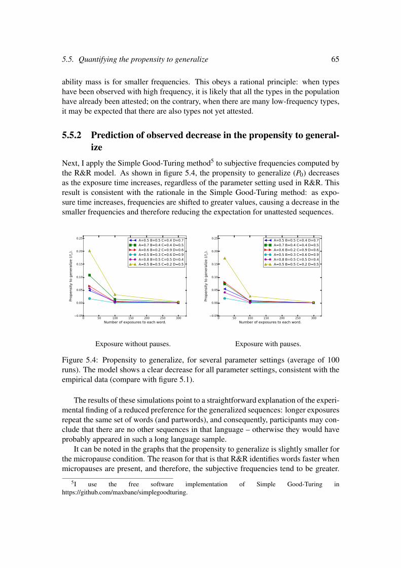
5.5. Quantifying the propensity to generalize 65
ability mass is for smaller frequencies. This obeys a rational principle: when typeshave been observed with high frequency, it is likely that all the types in the populationhave already been attested; on the contrary, when there are many low-frequency types,it may be expected that there are also types not yet attested.
5.5.2 Prediction of observed decrease in the propensity to general-ize
Next, I apply the Simple Good-Turing method5 to subjective frequencies computed bythe R&R model. As shown in figure 5.4, the propensity to generalize (P0) decreasesas the exposure time increases, regardless of the parameter setting used in R&R. Thisresult is consistent with the rationale in the Simple Good-Turing method: as expo-sure time increases, frequencies are shifted to greater values, causing a decrease in thesmaller frequencies and therefore reducing the expectation for unattested sequences.
0 50 100 150 200 250 300Number of exposures to each word.
0.05
0.00
0.05
0.10
0.15
0.20
0.25
Prop
ensit
y to
gen
eral
ize (P
0).
A=0.5 B=0.5 C=0.4 D=0.7A=0.7 B=0.4 C=0.4 D=0.5A=0.6 B=0.2 C=0.9 D=0.6A=0.5 B=0.3 C=0.6 D=0.9A=0.8 B=0.5 C=0.5 D=0.4A=0.5 B=0.5 C=0.2 D=0.5
Exposure without pauses.
0 50 100 150 200 250 300Number of exposures to each word.
0.05
0.00
0.05
0.10
0.15
0.20
0.25
Prop
ensit
y to
gen
eral
ize (P
0).
A=0.5 B=0.5 C=0.4 D=0.7A=0.7 B=0.4 C=0.4 D=0.5A=0.6 B=0.2 C=0.9 D=0.6A=0.5 B=0.3 C=0.6 D=0.9A=0.8 B=0.5 C=0.5 D=0.4A=0.5 B=0.5 C=0.2 D=0.5
Exposure with pauses.
Figure 5.4: Propensity to generalize, for several parameter settings (average of 100runs). The model shows a clear decrease for all parameter settings, consistent with theempirical data (compare with figure 5.1).
The results of these simulations point to a straightforward explanation of the experi-mental finding of a reduced preference for the generalized sequences: longer exposuresrepeat the same set of words (and partwords), and consequently, participants may con-clude that there are no other sequences in that language – otherwise they would haveprobably appeared in such a long language sample.
It can be noted in the graphs that the propensity to generalize is slightly smaller forthe micropause condition. The reason for that is that R&R identifies words faster whenmicropauses are present, and therefore, the subjective frequencies tend to be greater.
5I use the free software implementation of Simple Good-Turing inhttps://github.com/maxbane/simplegoodturing.

66 Chapter 5. Modelling the Propensity to Generalize
This might appear unexpected, but it is in fact not contradicting the empirical results:as shown in figure 5.3, the difference between words and partwords is much bigger inthe condition with micropauses, so this effect is likely to override the small probabilitydifference (as would be confirmed by a model of step (iii)). It should be noted that,as reported in Frost and Monaghan [2016], micropauses are not essential for all typeof generalizations (as is evidenced with the fact that rule*-words are generalized inthe no-pause condition). Like those authors, I think the role of the micropauses is toenhance the salience of initial and final syllables (A and C) to compensate for the oddconstruction of the test items (rule-words and class-words), which include a middlesyllable that occupied a different position in the familiarization stream.
5.6 DiscussionThe experiments I have focused on are all based on the same simple language, butthe results form a complex mosaic: generalization is observed in different degreesdepending on the amount of exposure, the presence of micropauses and the type ofgeneralization (rule-words, class-words or rule*-words). I have approached the analy-sis of these results with the use of several tools: first, with the three-step approach, aconceptualization of generalization that identifies its main components; second, withthe use of R&R, a probabilistic model that already predicts some aspects of the results—and, importantly, generates a skewed distribution of subjective frequencies that iscrucial for step (ii); and third, with the Simple Good-Turing method for quantifyingthe propensity to generalize. I now discuss how I interpret the outcome of my study.
Framing generalization with the three-step approach allowed us to identify a stepthat is usually neglected in discussions in ALL, namely, the computation of the propen-sity to generalize. I state that generalization is not only a process of discovering struc-ture: the frequencies in the familiarization generate an expectation about the probabil-ity of next observing any unattested item, and the responses for generalized sequencesmust be affected by it. Moreover, this step is based on statistical information, provingthat — contrary to the MoM hypothesis — a statistical mechanism can account for thenegative correlation with exposure time.
It should be noted that this conclusion concerns the qualitative nature of the learn-ing mechanism that is responsible for the experimental findings. It has been postulatedthat such findings evidence the presence of multiple mechanisms [Endress and Bonatti,2016]. In my view, the notion of ‘mechanism’ is only meaningful as a high-level con-struct that may help researchers in narrowing down the scope of the computations thatare being studied, among all the computations that take place in the brain at a giventime. After all, there is no natural obvious way to isolate the computations that wouldconstitute a single ‘mechanism’, from an implementational point of view. Therefore,the three-step approach should be taken as sketching the aspects that any model of gen-eralization should account for, and the work reported here show that the experimentalresults are expected given the statistical properties of the input.
5.6. Discussion 67
One issue to discuss is the influence of the use of the R&R model in computing thepropensity to generalize. The Simple Good-Turing method is designed to exploit thefact that words in natural language follow a Zipfian distribution —that is, languagesconsist of a few highly frequent words and a long tail of unfrequent words. This is akey property of natural language that is normally violated in ALL experiments, sincemost of the artificial languages used are based on a uniform distribution of words (butsee Kurumada et al. 2013). But it would be implausible to assume that subjects extractthe exact distribution for an unknown artificial language to which they have been onlybriefly exposed. R&R models the transition from absolute to subjective frequencies,resulting in a distribution of subjective frequencies that shows a great degree of skew,and much more so than alternative models of segmentation in ALL. Thanks to thisfact, the frequency distribution over which the SGT method operates (the subjectivedistribution) is more similar to that of natural language, and the pattern of results foundfor the propensity to generalize crucially depends on this type of distribution.
Finally, I have thus accomplished my goal qualitatively. The model captures thedownward tendency of the propensity to generalize, but a model for step (iii), a long-standing question in linguistics and cognitive science, is required to also achieve aquantitative fit. The next chapters review the existing models for such step, and presenta neural network model that reveal key properties of the generalization mechanism.

Part III
Generalization
69

Chapter 6Computational Models of Rule Learning
This part of the dissertation addresses the third step of the conceptualization I proposed;namely, how individuals generalize to novel items. First of all, in this chapter1 I presenta critical review of models of generalization, and reflect on what is missing and whichsteps should be taken in future research. I then present a new model in chapter 7 thataddresses some of the points raised in this review.
6.1 IntroductionOne of the key abilities of human cognition is the capacity for discovering regularitiesin the environment and generalize them to novel cases. For instance, consider how,after seeing a giraffe for the first time, we are able to conclude that a previously un-encountered giraffe is a member of the same animal species. Another well knownexample, introduced by [Fodor and Pylyshyn, 1988], is that an individual who under-stands the sentence John loves Mary can also understand Mary loves John2. To achievethat, an individual must abstract from the concrete properties in the input, and decidethe extension of novel items to which the abstracted regularity or rule applies to.
In experimental linguistics, and concretely in the tradition of Artificial LanguageLearning (ALL), the study of how structural relations are generalized from language-like input is known as rule learning3. In the last two decades, a great body of experi-mental work has emerged, focusing on how humans discover relations that range from
1The content in this chapter is based on the following manuscript:Alhama and Zuidema [2017c]. Computational Models of Rule Learning. [To be submitted.]
2Fodor and Pylyshyn refer to this property of human thought as systematicity. I see it as an instanceof a generalized relation between two items (the lover and the loved).
3The term rule learning can be easily misinterpreted, since it has also been coined to postulate aspecific theory of generalization (which I present later), according to which the knowledge extractedin such experiments must be explicitly represented as an algebraic symbolic rule. Unless otherwisespecified, my use of rule learning is interchangeable with generalization; and rule is by default used toconvey the same meaning as pattern or regularity unless it appears in the context of the specific theorythat postulates algebraic rules.
71

72 Chapter 6. Computational Models of Rule Learning
identity rules [Marcus et al., 1999, Gerken, 2006, Endress et al., 2007] to nonadjacentdependencies [Pena et al., 2002, Gomez, 2002, Gomez and Maye, 2005, Endress andBonatti, 2007, Frost and Monaghan, 2016] and even finite state grammars [Gomez andGerken, 1999].
These experiments have inspired a number of computational models that aim toprovide an explanation of the cognitive mechanisms underlying the empirical results.In this chapter, I focus on the experimental study presented in Marcus et al. [1999],which inspired a great number of modelling approaches and a very active debate aroundtheoretical issues such as the nature of the representations involved.
This chapter is structured as follows. First I describe the empirical findings fromthe experiment by Marcus and colleagues (§ 6.2). Then I describe the existing models(§ 6.3, § 6.4), to then identify what are the relevant questions that the models address(§ 6.5). Finally, I delineate an agenda of concrete desiderata for future modellingefforts (§ 6.6).
6.2 The Empirical DataMarcus et al. [1999] presented an ALL study that aimed to investigate the acquisitionof grammar-like rules by 7 month old infants. The authors run a total of three experi-ments, in which the 7 m.o. participants are familiarized with a speech stream consistentwith a certain ‘grammar’ or pattern. For instance, one of the familiarization streamscould involve syllable triplets like “linali talata nilani gagiga ...” (where the spacesdenote silence gaps); in this case, we say that the stimuli were generated with an ABAgrammar. In order to see if infants learn to extract the grammatical rule, they are subse-quently tested with stimuli that involve triplets consistent with the grammar they werefamiliarized with, and triplets generated with another control grammar. The amount oftime that infants direct their attention to the stimuli being played (the ‘listening times’)are recorded, and then a statistical test is applied to see if they are significantly differentbetween stimuli of the different grammars, showing in this case that infants learnt todiscriminate stimuli of each grammar. Crucially, the test stimuli contain syllables thatdid never appear in the familiarization stream; in this way, infants cannot solve the taskby only memorizing the syllables they were familiarized with.
In the first experiment, half of the participants are assigned to one of two conditions,differentiated by the grammar used to generate the familiarization stimuli: either ABAor ABB. After the familiarization phase, infants are tested to see if they extracted theunderlying grammatical patterns. In accordance to the procedure described above, forall the participants the test stimuli contain triplets from both the ABA and the ABBcondition. The complete stimulus set is listed in table 6.1.
A statistical analysis of the results of this first experiment shows that looking timeswere significantly longer for inconsistent triplets, reflecting what the authors interpretas a novelty preference. It seems therefore that infants are able to discriminate betweengrammatical and ungrammatical items. Since the syllables in test and familiarization

6.2. The Empirical Data 73
do not overlap, the results seem to be an indication that the infants have abstracted thegrammatical rule.
Familiarization TestABA ga ti ga li ti li ni ti ni ta la ta wo fe wo
ga na ga li na li ni na ni ta ti ta de ko dega gi ga li gi li ni gi ni ta na taga la ga li la li ni la ni ta gi ta
ABB ga ti ti li ti ti ni ti ti ta la la wo fe fega na na li na na ni na na ta ti ti de ko koga gi gi li gi gi ni gi gi ta na naga la la li la la ni la la ta gi gi
3x triplet (random order)
Table 6.1: Stimuli used in experiment 1 in Marcus et al. [1999].
Familiarization TestABA le di le wi di wi ji di ji de di de ba po ba
le je le wi je wi ji je ji de je de ko ga kole li le wi li wi ji li ji de li de
le we le wi we wi ji we ji de we deABB le di di wi di di ji di di de di di ba po po
le je je wi je je ji je je de je je ko ga gale li li wi li li ji li li de li li
le we we wi we we ji we we de we we3x triplet (random order)
Table 6.2: Stimuli used in experiment 2 in Marcus et al. [1999].
However, the authors identified a possible confound: the consonants in the stimuliappear always in voiced – unvoiced – voiced combinations, so the results could poten-tially be explained also as caused by the detection of such a pattern. In order to ruleout this possibility, a more carefully controlled replication of the previous experimentis presented (the list of stimulus items is shown in table 6.2). The responses in this ex-periment still prove to be statistically significant in discriminating between grammars,and therefore, the conclusions are consistent with those of experiment 1.
Finally, there still exists the possibility that the infants focus on the presence orabsence of an immediate repetition, rather than on the abstract identity rule. Therefore,the authors carry out a third experiment in which the stimuli grammars are ABB andAAB. Again, the participants show significantly different responses between gram-mars, so this alternative explanation is ruled out.
To summarize, the three experiments show significantly different responses foreach of the tested grammars, so it seems that infants find some regularity that allows
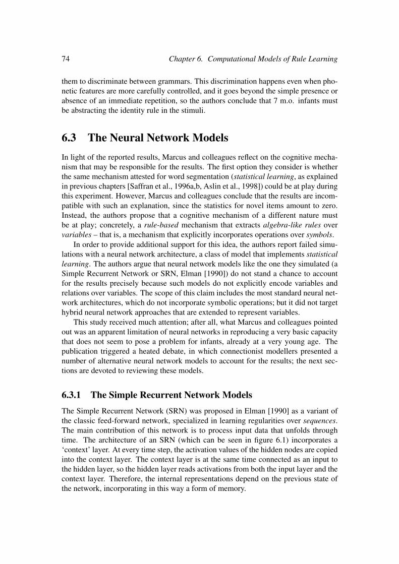
74 Chapter 6. Computational Models of Rule Learning
them to discriminate between grammars. This discrimination happens even when pho-netic features are more carefully controlled, and it goes beyond the simple presence orabsence of an immediate repetition, so the authors conclude that 7 m.o. infants mustbe abstracting the identity rule in the stimuli.
6.3 The Neural Network ModelsIn light of the reported results, Marcus and colleagues reflect on the cognitive mecha-nism that may be responsible for the results. The first option they consider is whetherthe same mechanism attested for word segmentation (statistical learning, as explainedin previous chapters [Saffran et al., 1996a,b, Aslin et al., 1998]) could be at play duringthis experiment. However, Marcus and colleagues conclude that the results are incom-patible with such an explanation, since the statistics for novel items amount to zero.Instead, the authors propose that a cognitive mechanism of a different nature mustbe at play; concretely, a rule-based mechanism that extracts algebra-like rules overvariables – that is, a mechanism that explicitly incorporates operations over symbols.
In order to provide additional support for this idea, the authors report failed simu-lations with a neural network architecture, a class of model that implements statisticallearning. The authors argue that neural network models like the one they simulated (aSimple Recurrent Network or SRN, Elman [1990]) do not stand a chance to accountfor the results precisely because such models do not explicitly encode variables andrelations over variables. The scope of this claim includes the most standard neural net-work architectures, which do not incorporate symbolic operations; but it did not targethybrid neural network approaches that are extended to represent variables.
This study received much attention; after all, what Marcus and colleagues pointedout was an apparent limitation of neural networks in reproducing a very basic capacitythat does not seem to pose a problem for infants, already at a very young age. Thepublication triggered a heated debate, in which connectionist modellers presented anumber of alternative neural network models to account for the results; the next sec-tions are devoted to reviewing these models.
6.3.1 The Simple Recurrent Network ModelsThe Simple Recurrent Network (SRN) was proposed in Elman [1990] as a variant ofthe classic feed-forward network, specialized in learning regularities over sequences.The main contribution of this network is to process input data that unfolds throughtime. The architecture of an SRN (which can be seen in figure 6.1) incorporates a‘context’ layer. At every time step, the activation values of the hidden nodes are copiedinto the context layer. The context layer is at the same time connected as an input tothe hidden layer, so the hidden layer reads activations from both the input layer and thecontext layer. Therefore, the internal representations depend on the previous state ofthe network, incorporating in this way a form of memory.
6.3. The Neural Network Models 75
Figure 6.1: The Simple Recurrent Network [Elman, 1990]. Dotted lines representtrainable connections; continuous line represents a one-to-one copy of the activationvalues.
As mentioned before, Marcus and colleagues report failed simulations with thismodel; however, other researchers proposed to model the experiment with an SRNwith certain modifications. I now review these models.
Using analog encoding
Negishi [1999] reflects that the lack of generalization in the original simulations is dueto the fact that both of the encoding schemes employed are based on binary activations.Instead, the author proposes to represent features of the input as real numbers.
The original simulations were replicated, but with the stimuli characterized by twocontinuous (analog) values: vowel height and place of articulation. This resulted in amodel that produced larger prediction errors for the grammar it was not trained with,a fact that may be interpreted as reproducing the increased attention over inconsistenttest stimuli observed in the experiment.
Marcus [1999c] argues that the use of analog encoding can be seen as endowing thenetwork with registers: if an input node represents all possible values, then it sufficesto connect it to the output node with a weight of 1, and thus, the node would act likea variable that instantiates a particular value at a given time. However, this reasoningis not so straightforward when it applies to SRN models: the non-linearities in thehidden layer, and the connection with the recurrent layer do not permit the direct copyproposed by Marcus. As argued in Sirois et al. [2000], variable bindings are onlyeffective if they can be accessed for further computation.
Optimizing for a different goal: Segmentation, Categorization and Transfer Learn-ing
Christiansen and Curtin [1999] (and later also Christiansen et al. [2000]) suggest thatthe statistical knowledge that infants acquire when attempting to segment the speech
76 Chapter 6. Computational Models of Rule Learning
in their environment could be the basis for their success in the experiment reportedby Marcus and colleagues. To prove this point, they use an existing SRN modelthat learns to segment speech using different types of probabilistic information [Chris-tiansen et al., 1998].
Their model is presented with a sequence of phonemes (instead of syllables), en-coded with phonological features, primary and secondary stress, as well as whether thephoneme is the last one in a triplet (and therefore it is followed by a 1s silence gap;see table 6.3 for more details). The model is trained to predict an arbitrary representa-tion of the next phoneme in the sequence, but also whether the phoneme is a syllableboundary, that is, whether it is followed by a 250s silence gap (which is the length forpauses within triplets). In this way, the model is expected to learn to segment syllablesafter having been given the information of triplet boundaries.
In order to evaluate the performance of the model, the authors introduce two novelmethods. First, they report that the network performs better at segmenting syllablesbelonging to triplets that are not consistent with the training grammar. The authorsinterpret this as accounting for the behavior of infants in the experiment, who pay moreattention to inconsistent test items. Second, an analysis of the internal representationsbuilt by the model is performed. The authors find that the representations for consistentand inconsistent triplets are distinguishable, as revealed by a two-group discriminantanalysis.
Marcus [1999c] argues that an analysis of the internal representations is not a suit-able evaluation, since representations must have a causal effect on the output in orderto be meaningful. Although the segmentation task could potentially account for that,Marcus observes that it is somewhat unnatural that the model is trained with stimulithat represents the pauses between triplets while being tested on the type of pausesthat have intentionally not been coded. Additionally, Marcus observes that the statisti-cal significance of the analysis of the internal representations may not be meaningful,since the test consists of a very small number of items (4) compared to the number ofhidden units (80) that provide the internal representation.
∗ ∗ ∗
The next model I review (Altmann and Dienes [1999], based on an earlier modelby Dienes et al. [1999]) conceives of generalization as an instance of transfer learningbetween different domains. In the context of the Marcus et al. experiment, the authorsidentify the domains as defined by familiarization stimuli and test stimuli. In order toaccount for the distinct domains, the authors extend the SRN architecture; concretely,the input and the output layers are augmented with extra nodes, such that two separategroups of nodes in each layer account for each domain. Additionally, the SRN isextended with an extra layer (the “encoding” layer), situated between the input and thehidden layer. The architecture of this network can be seen in figure 6.2.
The network is first trained as a normal SRN, using only the input and outputnodes of the first domain (D1). In the test phase, the stimulus is presented to the

6.3. The Neural Network Models 77
Figure 6.2: SRN model in Altmann and Dienes [1999] (image from Dienes et al.[1999]; copyrights remain with the original holders).
group of input nodes corresponding to the second domain (D2). Crucially, the testitems are presented several times, and – contrary to the previously reviewed models –the network continues updating the weights, with the exception of those connecting theencoding layer and the hidden layer, which remain “frozen”. By keeping those weightsintact, the model preserves some of the knowledge learnt during training and attemptsto transfer it to the test stimuli.
The authors measure the success of the network by computing the Euclidian dis-tance between the predicted and target vectors, for the vectors resulting from the lastiteration in the test. The results show higher correlations for prediction in the consis-tent grammar. However, Marcus [1999e] observes that this implementation is consis-tent with the experimental results only when evaluating the results by computing thedistance to the target. If, instead, one evaluates the most active unit in the predictedvector, then the model oscillates between the two grammars.
Additionally, it must be noted that in this model the domains are predefined, andthere is no a priori reason for the test items to be part of a different domain. Accord-ingly, the model requires a mechanism that selects and freezes a subset of the weights,but it is not clear when and under what circumstances this mechanism would oper-ate, and which particular subset of weights it should freeze. As Marcus puts it, themodel is task-specific, and it remains unclear how it can be related to other cognitivemechanisms.
∗ ∗ ∗

78 Chapter 6. Computational Models of Rule Learning
I now review a model that deviates from the original simulations in two ways: bychanging the task into categorization, and by accounting for prior experience. Sei-denberg and Elman [1999a] observe that the SRN presented by Marcus et al. had noprevious knowledge, while infants in their experiment had been exposed to naturallanguage in their environment. The authors argue that, by this prior exposure, infantsmight have learned to represent phonological similarity between syllables.
In order to account for prior knowledge, the authors extensively pre-train an SRNwith 120 different syllables. In this pre-training phase, one single node is optimized tooutput whether the current syllable is the same as the previous syllable in the sequence.In this way, the SRN is trained to learn identity between syllables.
The weights learned during pre-training are used to initialize the SRN for the ac-tual experiment, which is also defined as a categorization task, this time involving adifferent output node. Crucially, the network is not trained only with items belongingto one type of grammar (as the infants in the original experiment), but also with tripletsgenerated from both ABA and ABB.
When tested with the novel triplets, the network shows responses close to zero forthe ABA triplets and closer to 1 for ABB (concretely, 0.004 and 0.008 for bapoba andkogako, and 0.853 and 0.622 for bapopo and kogaga). Thus, it seems that the SRNlearnt to correctly discriminate between the grammars.
However, although the incorporation of pre-training is cognitively motivated, otheraspects of this work require further justification, as discussed also in response lettersMarcus [1999c], Seidenberg and Elman [1999b], Marcus [1999d]. The simulationsgreatly deviate from the original experiment in providing the model with negative evi-dence, and additionally, the incorporation of a feedback signal both during pre-trainingand training does not have its counterpart in the original experiment, since subjects inthe experiment did not receive any form of feedback.
Marcus further observes that the output node is trained to follow the symbolic rule‘if X==Y then 1 else 0’, suggesting that this evidences the need for symbolic opera-tions. Although the model is clearly trained under that rule, as Seidenberg and Elmanargue, the feedback is an external signal, which does not modify the space of hypoth-esis of the model. In other words, the fact that the supervision signal can be expressedwith a symbolic rule does not entail that the network implements symbolic operations.It is nevertheless not clear where the signal for learning identity on the first place wouldcome from, and whether it is plausible that a region of the brain is dedicated to findingidentity relations in the input.
Accounting for previous experience
I now review a model that also incorporates prior experience, but in this case it remainsas the original prediction task.
Altmann [2002] simulates the experiment in the same architecture presented inDienes et al. [1999] and Altmann and Dienes [1999] (reviewed in section 6.3.1). Likein the previous proposals, the model is allowed to learn during the test phase; however,

6.3. The Neural Network Models 79
in this study, no connections are frozen — that is, all the connection weights of themodel can be updated.
The pretraining consists of a prediction task over a set of 252 sentences in naturallanguage, which were generated from the grammar and vocabulary presented in Elman[1990] (with an additional control experiment that avoids sentences involving ABAor ABB structures). After the pretraining, the network is trained on the Marcus et al.stimuli, and then tested with the novel items.
The output of the model is evaluated by computing the product moment correla-tion between the predicted vector with the correct one. Statistical tests show that theresponse of the model significantly varies between consistent and inconsistent items.The authors conclude that their model reproduces the empirical data; however, the cri-tiques that Marcus raised for previous work [Marcus, 1999e], based on the fact that themodel iterates over the test items several times, apply also to these simulations.
Additionally, in my opinion a relevant aspect in this model is the type of representa-tion employed for pauses. The authors use two different vectors to encode the pauses:one for pauses that precede the onset of a triplet, and another to mark the ending. In thisway, the learning process can exploit this information to detect different associationsfor onset and final syllables. This constitutes an indirect form of positional informationthat is not available in the actual familiarization stream (since, perceptually, there is asingle uniform silence gap between triplets).
6.3.2 Neural Networks with non-sequential inputI now review two neural network models that are based on a different architecture,known as autoencoder or autoassociator [Mareschal and French, 1997]. These modelsdo not incorporate recurrent connections to learn sequential relations over the input;instead, they are optimized to find a suitable encoding of the input. The objectivefunction is set to minimize the error in reproducing the input pattern in the output, sothe network needs to built intermediate representations that favour the reconstructionof the input.
I first review the study presented in Shultz [1999] (later replicated in Shultz [2001]with a different encoding scheme). This model is an autoencoder that is trained withcascade-correlation [Fahlman and Lebiere, 1990]. The main property of cascade-correlation is that it gradually adds new nodes to the hidden layer, as determined by thecomputed error. Since the network is trained to reproduce the input in the output layer,the error signal is based on the difference between the actual output and the input.
In the original simulations, each syllable is encoded as a real number, which isrepresented in a single node. The information is presented to the network as triplets;thus, the input and output layers consist of 3 nodes, each one corresponding to onesyllable.
For the evaluation of the results, the author submits the error produced in the outputlayer to a repeated ANOVA. The results show a significant effect on grammar condi-tion, with more error for inconsistent test items. Shultz concludes that this reproduces

80 Chapter 6. Computational Models of Rule Learning
the original experiments, since more error requires further cognitive processing –aswould be reflected in the increased looking times for inconsistent items.
Marcus [2001] argues that, due to using just one node to represent each syllable,the model can easily learn to copy the relevant syllables in the output. It is true thatgiven the topology of the network, which is is built on the go, it is easy to imaginethat with the incorporation of a few nodes, the input gets roughly copied in the output(although distorted with the non-linear function applied to the hidden nodes), but Vilcuand Hadley [2005] showed with further analysis that the network does not perform suchmapping.
Vilcu and Hadly further argued that these results are only replicable for this partic-ular stimuli; for ABA or ABB sequences that involve different phonemes, the model isunable to distinguish between the grammars. Additionally, the authors show that themodel does not generalize to stimuli encoded outside the range of the real numbersemployed in the encoding.
It must be noted that this network operates over full triplets, creating in this way asomewhat artificial treatment of a continuous input. The next model I review incorpo-rates a slightly more realistic treatment of time.
∗ ∗ ∗
Sirois et al. [2000] implement a fully connected neural network; that is, the nodesin the network are all connected to each other. The network is trained to reproduce ex-ternal input in its nodes, strengthening the connections in the nodes that have correlatedactivations.
This model contrasts with the previous approaches in its formalization of time.Each syllable in a triplet is presented to a different group of nodes, one at time. Afterthe three syllables in a triplet have been presented, the activations are reset. Addition-ally, the model implements activation decay. For instance, when the third syllable ofa triplet is presented, the first and second syllables still remain active, but their activa-tions are decreased (with the first syllable having weaker activation than the second).
As for the evaluation, Sirois analyses the number of presentations required for thetest items to be assimilated (i.e. to be accurately reproduced by the network). Theresults of this analysis exhibit a significant difference between consistent and inconsis-tent items; therefore, the authors interpret the results as showing that this model couldbe a possible explanation of the original experiment.
It must be noted though that one of the drawbacks of this approach is that its designis intimately tied to the actual experiment: the architecture would need to be adapted inthe case of input sequences with a different number of syllables, and the full activationreset is linked to the appearance of the highly salient 1s silence gaps in the input, but itis not clear how this would generalize to stimuli involving less perceptible silence gaps(if any).

6.3. The Neural Network Models 81
6.3.3 Neural Networks with a repetition detector
We now review three models that include some form of dedicated mechanism to detectrepetitions of syllables in the input.
Shastri and Chang [1999] present a model of the Marcus et al. experiment thatimplements a form of dynamic binding [Hummel, 2011]. The model, originally pre-sented in Shastri et al. [1993], is implemented as a neural network with two groups ofdedicated nodes for the input: one group that represents the phonetic features for aninput syllable, and another group with three nodes corresponding to each of the threepositions in a triplet. The idea behind dynamic binding is that the nodes of the twogroups activate in synchrony, and therefore the coincident activity can be exploited bythe network in order to learn the abstract pattern in the input.
This neural network model involves recurrent connections, but it is not imple-mented as a standard SRN. Instead, the model (illustrated in figure 6.3) clamps someinput activations and propagates the activity through the network. After some delay,a target (the “correct” activation of the positional information) is clamped in the net-work. The difference between the actual activations and the target is used to update theweights through gradient descent.
Crucially, during the presentation of each syllable, all the positional nodes in whichthe syllable appears are active in the target; for instance, for the stimulus ledile, the firstand the third positional nodes are both active on each presentation of le, and the secondpositional node is active during the presentation of di. It must be noted that, with theintroduction of this form of feedback, the model is provided with an actual mechanismfor detecting repetitions.
When it comes to the Marcus et al. experiment, the performance of the modelis evaluated by computing the mean squared error between the model activations ofthe positional nodes and the target. The error is considerably smaller for test itemsconsistent with the training grammar, and thus the model appears to reproduce theempirical findings. However, this type of evaluation is based on the actual relationslearnt by the model (since it employs a target based on a rule), rather than on theproduced output (the “behaviour”) of the model. Therefore, it cannot be comparedto the results in the experiment with infants without assuming that these are the rulesextracted in the experiment.
Shastri and Chang argue that this approach offers a plausible mechanism to im-plement rules via biologically inspired temporal synchrony. Thus, this model is notpresented as a counterargument to the claim by Marcus et al.; actually, Marcus [2001]reflects that this model implements temporal rather than spatial variables. However, asargued also in Shultz [2001], the design of the model is very tied to the actual experi-ment; additionally, the feedback is clearly unrealistic, in providing the model with theexpected outcome rather than with the available information in the input. Therefore, itdoes not really offer a reconciliation between symbolic and neural network models.
∗ ∗ ∗

82 Chapter 6. Computational Models of Rule Learning
Figure 6.3: Model presented in Shastri and Chang [1999] (image courtesy of the au-thors; copyrights remain with the original holders). The numbers indicate link delaysin the connections.
Gasser and Colunga [2000] also present a model that implements another form ofdynamic binding. The authors frame the problem as extraction of correlations from theinput; in their view, the reason why the correlations that infants learn during the exper-iment allow them to generalize to novel items is that those correlations are relationalinstead of content-specific.
This model – named PLAYPEN – is implemented as a generalized Hopfield net-work, that is, a fully connected neural network model in which weights are adjustedwith the Contrastive Hebbian Learning algorithm [Hopfield, 1984]. The network, il-lustrated in figure 6.4, is provided with dedicated units that detect sameness and dif-ference. Therefore, its task is to reinforce the correlations according to the relations ofsameness and difference found in the input.
As in the previous model, the authors assume dedicated nodes for each syllableposition in a triplet. Additionally, the model is augmented such that each unit has an“angle”. While the particular value of the angle is irrelevant, it provides an additionaldimension to the network, such that units with similar angle can be treated similarly.In this way, Gasser and Colunga implement a form of simplified dynamic binding.
The results of the experiment simulations with this model show that the relationalunits are more active for test items consistent with the training grammar. Therefore, thenetwork has strengthened the connections of the relations present in the familiarizationstimuli.
In spite of the claims of biological plausibility of the model, its actual implemen-

6.3. The Neural Network Models 83
Figure 6.4: The PLAYPEN model [Gasser and Colunga, 2000] (image courtesy of theauthors; copyrights remain with the original holders). Diamonds indicate differencerelations; ovals indicate sameness.
tation remains extremely tied to the actual task, since the model comes with pre-wiredrelations over explicit bindings. Still, the authors argue that their model does not qual-ify as a symbolic model, since variables in symbolic models are content-independent,while PLAYPEN is sensitive to feature similarity between the presented items. How-ever, while I agree that the model does not implement symbolic variables, it does in-corporate rules, and thus it embodies the assumption that infants are equipped with arepetition detector.
∗ ∗ ∗
The last model in this section is a variant of a recurrent neural network model thatalso incorporates a repetition detector. This approach, presented in Dominey and Ra-mus [2000], is based on an architecture called Temporal Recurrent Network [Dominey,1995], a recurrent architecture in which only the weights connecting the hidden andthe output layer are trained (while the rest are randomly initialized and remain un-changed). Interestingly, the nodes in this network are Leaky Integrate-and-Fire units.This endows the network with a more realistic representation of time: unlike in previ-ous approaches, in which activations consist of a single value that is produced after adiscrete timestep, the nodes of this network produces activations in the form of contin-uous spikes.
Nevertheless, the authors do not find with this model a pattern of results that isconsistent with behaviour of the infants in the experiment. Therefore, they explore anaugmented version of the model, which they call Abstract Recurrent Network (ARN).The ARN model features an additional short-term memory that stores the last 5 syl-lables of the input (in order to account for the 7±2 magical number for short-termmemory, [Miller, 1956]), and a “recognition” component that detects whether any ofthe items in the short-term memory is the same as the actual item. This information is

84 Chapter 6. Computational Models of Rule Learning
then provided to the internal state (the hidden layer), so that the model can exploit thisinformation while updating the weights between the hidden layer and the output.
Given that the model is updated in continuous time, the responses can be easilycompared to Reaction Times. Concretely, the authors measure the response latencies ofthe activation of the correct output nodes. These latencies should be smaller for learntitems, since the strength of the activations in the network would influence the activity inthe output. With this form of evaluation, the authors find significant statistical evidencefor shorter Reaction Times for test items consistent with the familiarization grammar.
This model therefore appears to be a promising approach, in incorporating suc-cessful learning with a more realistic treatment of time. However, as mentioned in theprevious approaches, this network is endowed with a component that actively looks forrepetitions in short-term memory (and even contains a node that fires when no repeti-tion is found). This results in the very strong postulation that infants must be equippedwith such dedicated mechanism.
Importantly, this model adds some form of variables, in line with the claims byMarcus and colleagues. This is due to how the model accesses the augmented short-term memory, which is based on isolated memory positions dedicated to store differentitems. It must be emphasized that this behaviour comes from how the memory is ac-cessed, not by the mere fact of adding short-term (spatial) memory; in other words, anetwork with this kind of memory may learn how to access it efficiently, and mighteventually discover how it can exploit that nodes in the memory are dedicated to dif-ferent items. This is not the case in the model by Dominey and Ramus, in whichthe recognition component is handcrafted to have positional access to elements in theshort-term memory.
6.3.4 Evaluating the Neural Network ModelsAlthough the models reviewed address the same experimental data, they greatly differin the criteria applied to judge their success in reproducing the empirical phenomenon.In the original simulations by Marcus and colleagues, it is not clear how the output ofthe model was evaluated, since the authors only report that “the network is unable todistinguish the inconsistent and consistent sentences”. In the follow-up papers, mod-ellers use some error measure (e.g. Mean Squared Error) to compute how much thepredicted vectors deviate from the target [Negishi, 1999, Altmann and Dienes, 1999,Altmann, 2002, Shultz, 1999, Shastri and Chang, 1999]; generally this is accompaniedwith a statistical analysis that shows whether the computed error allows for distinctionbetween grammars.
While that is the most common approach, the rest of the reviewed studies applycompletely different criteria. To begin with, Seidenberg and Elman [1999a] report theaverage activity of the output node in their model (which is trained for grammar classi-fication). Another example is Sirois et al. [2000], who compare the number of stimulipresentations required to succeed in generalization in each grammar. We find yet an-other approach in Gasser and Colunga [2000], who analyze whether the model learns

6.4. Symbolic Models of Rule Learning 85
the expected identity rule (an approach that is also present in an extended analysis inShastri and Chang [1999]). In contrast, Christiansen and Curtin [1999] and Chris-tiansen et al. [2000] evaluate their model in its prediction of the internal pauses withina triplet (since the authors frame the problem as a segmentation task). Additionally,the authors also analyze the internal representations built by the model, and find thatthey are distinguishable for each type of grammar. Finally, a contrasting approach isfound in Dominey and Ramus [2000], in which the latency of output node related tothe correct prediction is measured and taken as an indication of Reaction Time.
Given this stunning variation on evaluating the models, it is not possible to quanti-tatively compare the models in either their goodness of fit to the empirical data or in towhat extent the models are capable of generalization.
Interestingly, there is one aspect of the evaluation criteria on which most of theproposals agree: the models are evaluated in showing some form of discriminationbetween grammars. The corollary is that, even though a successful model can reliablydetect some difference between the stimuli generated by each grammars, it need not becapable of accurately generalizing (i.e. on systematically predicting or accepting novelitems that are consistent with the generalized rule). Exceptions to this are the modelsby Shastri and Chang [1999] and Gasser and Colunga [2000], which are evaluatedon learning abstract identity (or difference) relations –albeit they are not evaluated onproducing actual generalizations but rather on settling for the hypothesized rules.
6.4 Symbolic Models of Rule LearningAll the models reviewed so far are neural network approaches, albeit some of themincorporate some form of symbolic structure. The original proposal by Marcus andcolleagues can also be implemented in a purely symbolic model, but the number ofsuch models applied to the Marcus et al. experiment is really small (to the best of myknowledge, the only existing models are Kuehne et al. [2000] and Frank and Tenen-baum [2011]). A possible reason for this asymmetry with neural approaches is that thegrammars to be learnt are so simple when rules and variables are assumed that thereis not much room for unexpected findings. For this reason, here I focus on the modelby Frank and Tenenbaum [2011], since its the only model that goes beyond simplerule extraction to also address an important question that has been neglected in otherapproaches; namely, what determines which rule is preferred when there are multipleconsistent rules.
The model presented by F&T is a Bayesian model, inspired by the Bayesian simi-larity model in Tenenbaum and Griffiths [2001]; however, unlike the original proposal,it is not driven by analogy between exemplars; instead, the model infers the most likelysymbolic rule that may have generated the observed data.
The hypothesis space in this model consists of an inventory of symbolic rules.Since the model is applied to a variety of datasets, this inventory is adapted to eachexperiment; in the case of the experiment by Marcus and colleagues, the hypothesis

86 Chapter 6. Computational Models of Rule Learning
space incorporates an identity relation over syllables. Therefore, the model may learnany combination of identity relations over syllables in the input.
The model uses Bayesian inference to decide which is the most likely rule r (gram-mar) that may have generated the observed stream of triplets T = t1, ..., tn; in otherwords, the goal of the model is to find for which rule r the posterior probability p(r|T )is maximal. As defined in equation 6.1, the posterior can be computed as a product ofthe likelihood of observing the data assuming this rule p(T |r) (see equation 6.2) andthe prior probability of the rule p(r) (that is, the probability of a rule before observingthe input stream). In order for the posterior to be a probability, this product needs to benormalized by the sum of the probabilities for all possible rules.
p(r|T ) = p(T |r)p(r)∑r′∈R p(T |r′)p(r′)
(6.1)
where
p(T |r) = ∏ti∈T
p(ti|r), (6.2)
and where
p(ti|r) =1|r|
. (6.3)
The prior is defined as a uniform distribution; hence, each rule is a priori equallylikely. As for the likelihood, the authors assume strong sampling, that is, the tripletsare assumed to have been uniformly sampled from the set of triplets that a rule cangenerate. This entails that the probability of observing a triplet under a certain grammaris larger for “smaller” grammars (that is, grammars that generate a smaller number oftriplets), as seen in equation 6.3. This creates a bias in the model in favour of moreconcise grammars; for instance, for a triplet such as “je-li-je”, a rule like ABA is morelikely than a more general but equally consistent rule ABC that involves no identity.
Given the simplicity of the experiment and the model, the only rule that can com-pete with ABA or ABB is ABC, that is, a grammar which generates triplets consistingof three arbitrary syllables, which may or may not be repeated. This model shows thatmore probability is attributed to the more specific grammars ABA and ABB (consistentwith the size principle defined above).
The authors present two additional variants of this model: one that assumes a cer-tain amount of noise in the generative process (regulated through an additional parame-ter), and another that additionally allows for the possibility that the data was generatedfrom multiple rules.
Due to the addition of parameters, the model now requires a procedure of fitting.The posterior probabilities derived from the model are related to the human responsesthrough the use of the negative log probability (surprisal). These two models also at-tributed more probability (less surprisal) to the rules involving identity, although some

6.5. Analysis of the Models 87
small probability mass was attributed to the general rule ABC.Thus, the BLM model identifies which rules would be favoured under a rational
model incorporating a certain bias for less general rules. Although the model appearsextremely simple in comparison to the neural network approaches (mostly due to thefact that that the hypothesis space is relatively small and manually defined, ad hocfor the experiment), it brings an additional value that should not be underestimated.Concretely, it is the only model that clearly defines which biases are hypothesizedto guide the preference for certain rules over others. Thanks to that, this approachincorporates a principle that postulates why the participants induced an identity ruleinstead of a more general rule in which all triplets are possible.
This study was fiercely criticized in a follow up publication [Endress, 2013]. Amongother issues, the author questions the validity of the “size principle” as a cognitive bias.The author reports an independent experiment in which participants are exposed to in-stances of an ABB grammar, vocalized with human speech. The participants coulddiscover at least two rules: the identity rule between the second and third syllable, ora more general rule glossed as “any sequence of human speech syllables”. In the sub-sequent test phase, participants had to choose between an ABB sequence of monkeyvocalizations, or AAB triplets carried by human speech. The results show a preferencefor the AAB human triplets, a fact that is interpreted by Endress as contrary to the “sizeprinciple”. However, Frank [2013] argues that this data shows a modality preferencerather than a rule preference. The issue is therefore not settled: it is not clear whetherthe subjects prefer certain generalizations based on the “size” of the set of items thata rule can generate or based on a bias favouring acoustic aspects of the input (i.e. thevocalizations).
6.5 Analysis of the ModelsIn the previous section, I have reviewed models that appear to offer distinct perspec-tives on generalization. I now identify what I think are the most relevant questionsthat the Marcus et al. experiment give raise to, and analyse whether these seeminglycontrasting approaches differ in answering those questions.
6.5.1 Question 1: Which features or perceptual units participatein the process?
In the experiment, infants are exposed to a synthesized speech stream. The way thisstream is perceived must impact what is learnt from it, and therefore, details of this per-ceptual process are relevant. For instance, do infants perceive the input as a sequenceof phonemes, or is the syllable the most salient perceptual unit? Do they analyze lower-level properties, such as phonetic features, once a syllable has been recognized? Doother acoustic dimensions, such as loudness or pitch, play a role in what is learnt? Howdoes the insertion of silence gaps affect the perception of the basic units?
88 Chapter 6. Computational Models of Rule Learning
These questions have not received much attention. However, thanks to using com-puter modelling, researchers are forced to make choices on how to represent the inputand how to present it to the model over time. This is reflected in the encoding, whichmay, for instance, incorporate some detailed acoustic aspects of the stimuli or, instead,represent it with arbitrary symbol that does not encode any properties of the item. Thelatter is the approach taken by symbolic models such as the BLM, where each sylla-ble is represented with an arbitrary symbol that does not incorporate any informationof what it represents. But in the case neural network models, the input vector can becoded in either way, as explained next.
In a localist encoding scheme, vectors are initialized to a null value (typically, 0 or-1) except for one of its units, which will have a non-null activation value (typically,1). The position of the active unit indicates which item is represented, but it does notconvey any information of the properties of the item; therefore, localist representationsare always arbitrary. On the contrary, in a distributed encoding scheme, each unit mayparticipate in the representation of more than one item. Although these values canbe chosen arbitrarily, each unit may be chosen to represent one particular property ofthe item, and thus, the distributed vector would encode certain specific properties ofthe stimuli. As shown in table 6.3, models vary in the choice of represented acousticfeatures.
The choice of the encoding scheme has an impact on generalization. As argued inMarcus [1998], for a neural network to succeed in generalizing to novel items, suchnovel items must fall within the training space; that is, the values of each unit must havebeen witnessed by the network during training (even if in different combinations). Forinstance, if the training data contains the vectors [1, 1, 1], [1, 0, 1] and [1, 0, 0], thena novel item like [1, 1, 0] lies within the training space, while [0, 1, 0] is outsidethe training space, since the first unit in the vector has never taken the value 0 duringtraining. If a certain unit in the input always has the same value during training thenetwork learns a solution based on such fixed value, and therefore the solution will notbe valid for novel test items that contain the opposite feature value.
For this reason, the choice of the encoding scheme and the dimensions to encodeis relevant, since a certain amount of overlap is needed for generalization in neuralnetworks. To illustrate this, consider the case in which localist representations are used.The nodes that represent the test items will be zero during familiarization, and thereforethe learning algorithm will update the connecting weights until they converge to zero,so they would never be active to predict novel items. On the contrary, with distributedvectors, some of the units representing the test stimuli may have been active duringtraining.
This raises two relevant issues. First of all, distributed vectors stand a chance forgeneralization, depending on the overlap between vectors in training and test. This canbe accomplished in two ways: either by using pseudo-random symbolic initializationsthat guarantee a certain amount of overlap, or by investigating which are the relevantproperties of the input that need to be coded in the vector. To our knowledge, this issuehas not been thoroughly explored. Thus, this will be one of our points in the desiderata
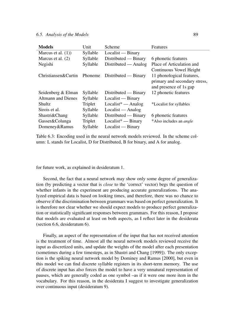
6.5. Analysis of the Models 89
Models Unit Scheme FeaturesMarcus et al. (1)) Syllable Localist — BinaryMarcus et al. (2) Syllable Distributed — Binary 6 phonetic featuresNegishi Syllable Distributed — Analog Place of Articulation and
Continuous Vowel HeightChristiansen&Curtin Phoneme Distributed — Binary 11 phonological features,
primary and secondary stress,and presence of 1s gap
Seidenberg & Elman Syllable Distributed — Binary 12 phonetic featuresAltmann and Dienes Syllable Localist — BinaryShultz Triplet Localist* — Analog *Localist for syllablesSirois et al. Syllable Localist — AnalogShastri&Chang Syllable Distributed — Binary 6 phonetic featuresGasser&Colunga Triplet Localist* — Binary *Also includes an angleDomeney&Ramus Syllable Localist — Binary
Table 6.3: Encoding used in the neural network models reviewed. In the scheme col-umn: L stands for Localist, D for Distributed, B for binary, and A for analog.
for future work, as explained in desideratum 1.
Second, the fact that a neural network may show only some degree of generaliza-tion (by predicting a vector that is close to the ‘correct’ vector) begs the question ofwhether infants in the experiment are producing accurate generalizations. The ana-lyzed empirical data is based on looking times, and therefore, there was no chance toobserve if the discrimination between grammars was based on perfect generalization. Itis therefore not clear whether we should expect models to produce perfect generaliza-tion or statistically significant responses between grammars. For this reason, I proposethat models are evaluated at least on both aspects, as I reflect later in the desiderata(section 6.6, desideratum 6).
Finally, an aspect of the representation of the input that has not received attentionis the treatment of time. Almost all the neural network models reviewed receive theinput as discretized units, and update the weights of the model after each presentation(sometimes during a few timesteps, as in Shastri and Chang [1999]). The only excep-tion is the spiking neural network model by Dominey and Ramus [2000], but even inthis model we can find discrete syllable registers in its short-term memory. The useof discrete input has also forces the model to have a very unnatural representation ofpauses, which are generally coded as one symbol –as if it were one more item in thevocabulary. For this reason, in the desiderata I suggest to investigate generalizationover continuous input (desideratum 9).

90 Chapter 6. Computational Models of Rule Learning
6.5.2 Question 2: What is the learning process?
One of the most relevant and ambitious scientific questions behind the Marcus et al.experiment is to understand the nature of the learning mechanism that is operatingduring the experiment. Since we only observe the input stimuli and the behaviouraloutput, the characterization of the unobserved procedure that relates them allows formultiple hypothesis.
In neural networks, the process of learning is commonly referred to as “associativelearning”, and it is characterized by responding to contingency relations in the data.Most neural networks are trained with some form of gradient descent; in the majorityof cases, the algorithm used is backpropagation [Rumelhart et al., 1988]. Althoughthe neurobiological plausibility of backpropagation was initially in question [Zipserand Andersen, 1988, Crick, 1989, Stork, 1989], later work argued that the learningprocedure can be implemented also with biologically plausible bidirectional activationpropagation [O’Reilly, 1996, 1998]; moreover, Xie and Seung [2003] prove that –under certain conditions– backpropagation is mathematically equivalent to ContrastiveHebbian learning, a process whose biological plausibility is widely agreed upon. Allthe neural network models reviewed implement some form of gradient descent, withthe exception of the proposal of Dominey and Ramus [2000], which features a learn-ing algorithm based on cortico-striatal circuits in the brain [Dominey, 1995], whichresearchers have interpreted as a form of Least Mean Squares [Lukosevicius, 2012].
In the rule-based model proposed by Frank and Tenenbaum [2011], the modellearns through Bayesian inference over a predefined space of hypothesis. Therefore,this model does not offer an account of the process that induces the regularities in thefirst place. However, the authors clearly state that the model is proposed as an “ideallearner” rather, and thus it should not be interpreted as a model of human learning.Therefore, a cognitively realistic rule-based model that explains how learning takesplace during the experiment is still lacking.
6.5.3 Question 3: Which generalization?
The speech streams we are concerned with are generated according to an ABA, AABor ABB pattern, which involves relations between syllables. However the stimuli arealso compatible with other rules, and – as discussed in section 6.5.1– regularities mayalso appear on other acoustic dimensions.
In order to illustrate this, table 6.4 shows some of the rules that describe the rela-tions between syllables in the triplets. These can be as general as ‘three consecutivesyllables’ (equivalent to rule (a)), or they could operate over two of the syllables in thetriplet. These basic rules can be composed with logical operators (and, or, not), suchas ‘(a) and (b)’; for instance, if a learner is hypothesized to learn a rule like ‘tripletcontaining an adjacent repetition’, this can be expressed as ‘X=Y or Y=Z’. As will beexplained in next section, theories that postulate that rules are cognitively real need todisambiguate which rule is being learnt when rules are equivalent in their extension.
6.5. Analysis of the Models 91
From the models have reviewed, only the Bayesian approach Frank and Tenen-baum [2011] explicitly tackles this question. In order to distinguish between otherwiseequiprobable consistent hypotheses, this model incorporates a predefined rational prin-ciple that determines which hypothesis should be favoured; in this case, the size prin-ciple. In this way, this model offers a transparent way to test how different principleswould be favoured by a probabilistic inference process, an aspect that is missing in theneural network models.
It must be noted that rational principles are not the only source of disambigua-tion to decide between competing rules. For instance, Endress et al. [2005] report ex-perimental evidence showing that repetition-based grammars are easier to learn whenthe repetition takes place in the edge positions. This entails that other aspects –suchas perceptual factors– can also impose saliency in certain dimensions of the stimuli,breaking the uniformity between otherwise equivalent rules. For this reason, I suggestin desiderata 2, 3 and 4 that alternative factors that influence why certain rules arefavoured should be explored.
6.5.4 Question 4: What are the mental representations created?Even if we agree on the generalization procedure and the question of which rule hasbeen extracted, we still need to discuss how the induced rule is represented in thecognitive system.
Symbolic and non-symbolic models have different strengths and weaknesses. Rule-based models exploit the fact that symbolic rules can easily accommodate some of themost interesting properties of thought and language, such as systematicity, productivityand compositionality. The use of variables that are blind to the specific propertiesof their content ensures a rigorous description: as well as a binary output: rules areeither consistent or inconsistent, never in between. However, this has the downside ofendowing the models with little flexibility, and thus they are not robust to noise [Opitzand Hofmann, 2015]. In contrast, neural network models do not explicitly representrules or variables, so relations are content-dependent (as well as context dependent).One of the advantages of these models is that they can naturally account for degradedinstances or accidental gaps; therefore, exceptions can be handled without the need ofadditional mechanisms [Elman, 1999].
As researchers, we are used to employ formal languages for scientific descriptions,and thus it is natural to characterize stimuli with formal rules such as XYZ such thatX=Z. And indeed, the behavior shown by the infants in Marcus et al. experiment can bedescribed as following an identity rule that accounts for the familiarization grammar.However, the mental representations of infants in the experiment need not directly mapwith the components of such formal expression: the variables and the logical operatorsthat relate them may or may not correspond directly to mental entities.
As argued in Pylyshyn [1991], it is common in science that a debate arises whenthe object of research involves a system that can be easily described with rules. Theauthor outlines a topology for theories addressing those type of systems, according to
92 Chapter 6. Computational Models of Rule Learning
which the ontological status of the theory can be seen as a point in a spectrum betweentwo extremes. Theories may, on one extreme, postulate rules that only account forregularities in the behavior of the system. In this case, rules function only as a theo-retical descriptive construct, but the theory is agnostic towards the representations andthe principles followed by the system. In intermediate positions, theories postulate thatsome of its elements correspond to principles or properties materialized in the system.And on the other extreme, theories maintain that all its rules and representations areexplicitly encoded in the system. In the latter case, the elements in the canonical ex-pression of a rule (including its symbols and the relations between them) correspondto certain properties in the system. Thus, details such as the total number of rules andtheir precise definition (e.g. whether they are based on identity or difference, even iftheir scope is identical) become relevant for a theory that posits that these rules arematerialized in the cognitive system.
This characterization of theories can be easily related to Marr’s levels of analysis[Marr, 1982]. Marr suggests a topology for computational models of cognition, suchthat: i) computational level theories are concerned only with characterizing the prob-lem and the solution, ii) algorithmic or processing level models propose a mechanisticaccount of the process and the representations in the cognitive system, and iii) imple-mentational level approaches explain how the process and representations are physi-cally instantiated. Thus, according to this characterization, computational-level modelsmay employ high-level descriptions that may not translate into actual representationsin lower levels.
With this taxonomy at hand, it is straightforward to see where the described modelsstand on such issue. The rule-based model in Frank and Tenenbaum [2011] is explicitlystated at Marr’s computational level; therefore, the fact that it employs symbolic rulesis not to be taken as a representational claim. On the other hand, neural networkmodels are implementational-level accounts of how processes and representations maybe realized. Thus, (most of) the reviewed neural network models propose that symbolicrepresentations are not cognitively real, and that the emergent behaviour observed inthe experiment can emerge even when symbolic representations are not employed.
6.5.5 Conclusion of the analysis
This analysis has allowed us to closely examine how this collection of models hashelped in advancing our knowledge on the main research questions. But surprisingly,in spite of the relative simplicity of the experiment and the vast number of models, thestate of our knowledge appears rather incomplete when we analyze the questions atthis level of detail. For this reason, I have compiled an agenda of the issues that requiremore attention.
6.6. An agenda for Rule Learning 93
6.6 An agenda for Rule LearningI now reflect on how the unresolved issues identified in our analysis could be mate-rialized in future studies, and I briefly mention some of the most recent work that isstarting to address my desiderata.
1. DESIDERATUM. Investigate which features should be encoded in the input repre-sentation, and quantify the overlap of features needed for generalization to occur.
To begin with, not much attention has been devoted to how the perception of theinput can affect generalization. The syllables in the original experiment are chosen tominimize phonetic overlap, but as pointed out by McClelland and Plaut [1999], otheracoustic cues may exhibit regularities. Additionally, similar experiments involving adifferent set of syllables show null results (Geambasu&Levelt, p.c.), suggesting thatlow-level cues are relevant.
As mentioned before (section 6.5.1), the amount of overlap in the representation ofinput vectors in neural network models influences the prediction of novel items. Thus,more research is needed to quantify the amount of overlap required to reproduce theempirical findings, and specially, which features should be encoded in the vectors (andtherefore, which perceptual dimensions guide generalization).
2. DESIDERATUM. Investigate perceptual biases.
The second issue that can be observed is that, in all models, the perceptual units(generally syllables) are treated equally, regardless of the position they appear in. How-ever, as mentioned before, experimental work shows that syllables that appear in theedge of sequences are more salient to humans, to the extent that some rules are notlearnt if the regularity appears in middle positions [Endress et al., 2005].
The reviewed models do not explicitly incorporate any such biases. Although acase could be made for neural networks being able to learn those biases, this wouldonly occur when saliency facilitates the task. Thus, I suggest that future efforts shouldbe directed to investigate which perceptual biases facilitate or hinder generalization.
3. DESIDERATUM. Investigate the role of prior experience.
Most of the models reviewed are used as a tabula rasa: they are initialized with someindependent method (e.g. randomly sampled weights in a neural network) and thentrained exclusively on the familiarization data. However, for a randomly initializedmodel, it is unlikely that a short exposure to the familiarization stimuli suffices to re-produce the experiments. If, instead, the initial state of the models incorporates relevantprior knowledge, the learning procedure may converge more easily to the generalizingsolution that infants seem to learn.
This is the idea behind the models proposed by Altmann [2002] and Seidenbergand Elman [1999a], but our analysis concluded that these models are not convincing

94 Chapter 6. Computational Models of Rule Learning
explanations of the empirical phenomenon. Moreover, the use of pretraining proce-dures would result more explanatory if the they allow to pinpoint which aspects of theprior knowledge are the ones influencing generalization to novel items.
4. DESIDERATUM. Model the coexistence and competition of rules.
It is very unlikely that a perceived flow of information can be described with onesingle rule, but rather, an input stream is likely to incorporate regularities betweenfeatures in different dimensions. Thus, a model of generalization should explain howthe detected regularities coexist, that is, how they are represented and whether theyinterfere between each other during the course of perception and learning.
In reviewing the existing models of generalization of simple grammars, I have ob-served that the question of “which generalization” has been widely neglected. TheBayesian model by Frank et al. has initiated that an approach to that question byproposing the size principle as a rational criteria to predict a preference for some rulesover others (see also Chater and Vitanyi [2003] for an more general argument for sim-plicity as the disambiguating rational principle). However, I argue that factors otherthan rational principles of parsimony may also play a role.
Some of the desiderata outlined above suggests factors that may influence the pref-erence for some rules, such as perceptual factors like edge saliency, or the role of priorexperience in shaping the perceived contingencies (or in providing the right pressurefor finding generalising solutions). External factors may also play a role; for instance,the contextual information.
As an example, consider a math student who is asked to generalize after seeingnumbers 30 and 40: we would expect her to be more likely to generalize to number50 than to 41, inducing a mathematical rule such as ‘multiple of 10’. But a medicinestudent who is studying dangerous cholesterol levels, after observing that 30 and 41 area dangerous levels, would prefer to generalize to 41 rather than 50, due to proximity.Given the same input, and the task of generalizing to novel stimuli, the context providesextraneous cues that have an effect on the favoured generalizations (example adaptedfrom [Tenenbaum and Griffiths, 2001]).
To sum up, I suggest that future models attempt to explain how rules coexist andcompete, and aim to reveal which factors determine which rules are preferred.
5. DESIDERATUM. Incorporate independently motivated pressures for learning gen-eralizing solutions.
The hypothesis space in neural networks often contains multiple local optima, andthus the learning procedure has high risk of getting stuck in one of those local optima.This entails that, in practice, there exist multiple solutions that may be found by a neu-ral network model. While these solutions can be sufficient to account for the trainingdata, they may not be generalising solutions that can be transferred to the test stimuli.
This can be seen as a form of overfitting. Since neural networks have many degreesof freedom, they can easily find one of the non-generalizing solutions. In order to push
6.6. An agenda for Rule Learning 95
a neural network model to find a generalizing solution, an additional source of pressureis needed. Thus, I believe an important avenue of future research is to investigate howto incorporate independently motivated biases to find generalizing solutions.
6. DESIDERATUM. Find a consensus in evaluation criteria for models.
One of the most pressing issues that I have discovered in this review is that there isample disagreement in the formulation of the objective to optimize and, specially, onhow to evaluate the outcome of a model.
As I observed before, reflecting on the evaluation reveals an important issue aboutthe empirical data: while the results exhibit statistical significance for the attention thatinfants show between different grammars, there is no evidence that infants performaccurate generalization (i.e. correct prediction of the last syllable in a triplet). It iscertainly ambitious to establish the reality for the subjects in the experiment, since wedo not know of experimental procedures that allow us to investigate what exactly haveinfants learnt. Progress in this direction would definitely facilitate that modellers settlefor one particular evaluation method and compare the different model proposals in asystematic manner.
For lack of better knowledge, I suggest that models are evaluated on both crite-ria: i) whether they exhibit statistical significance for grammar discrimination, and ii)whether the model accurately generalizes to new items.
7. DESIDERATUM. Bridge the gap between levels of analysis: investigate how neuralnetworks perform apparently symbolic computations.
As discussed before, one of the most debated issues is the ontological status ofsymbolic rules and variables. Even though the neural network models reviewed havearguably shown some success in reproducing the empirical findings, the relation be-tween the symbolic-like behaviour and its actual realization in the model is not com-pletely clear: neural networks are assumed to perform symbolic-like computationsimplicitly, but how exactly this is done remains elusive. Thus, in order to understandhow non-symbolic systems perform apparently symbolic computations, we should aimto investigate the internal representations and strategies employed by neural networks.
This issue can be regarded as finding the relation between computational level ex-planations (for which rules and symbols are well suited) and the corresponding imple-mentational realization. Thus, another way to frame this problem is in trying to bridgethe gap between the computational level approaches (such as those offered by Bayesianmodels) and implementational models.
8. DESIDERATUM. Models should learn spontaneously from brief/limited exposure.
Neural network models need to iterate over the data in order to converge to a goodparameter setting. This is aggravated in the case of small training datasets (as wouldbe the case for the Marcus et al. stimuli), since less data entails that more epochs

96 Chapter 6. Computational Models of Rule Learning
are required for convergence. Unfortunately, this does not reproduce the training setup used in the infants experiment, in which the familiarization stimuli is presentedonly once. Although it could be argued that the iterations of the stimuli reflected theavailability of the data in short term memory (such as the phonological loop), this doesnot allow us to distinguish between tasks that can be learnt spontaneously and thosethat require a longer exposure or even a developmental trajectory.
For this reason, I think that achieving spontaneous learning with neural networkmodels is an ambitious but relevant project. Recent advances on neural network archi-tectures involving augmented memory (e.g. the Neural Turing Machines [Graves et al.,2014]) are capable of fast memorization and retrieval of input stimuli, and thus theyoffer a promising avenue for learning from short-exposures (e.g. successes in one-shotlearning have been reported in Santoro et al. [2016]).
9. DESIDERATUM. Investigate the effect of the continuous nature of speech in gener-alization.
An aspect that has been widely neglected in the reviewed models is to represent thecontinuous nature of speech. Some of the models operate over all the data at once (con-cretely, the Bayesian model), while the neural networks process the data in an onlinefashion, either over triplets, syllables or phonemes. But even in this case, the streamis pre-segmented, and the models are updated synchronously in discrete timesteps –although, as argued in section 6.3.3, the model by Dominey and Ramus [2000] offersa more realistic treatment of time, but it does not succeed in modelling the experimentwithout pre-segmenting the input syllables and accessing its storage in a symbolicfashion.
By simplifying the representation of time, some aspects of auditory processing canbe neglected. For instance, the speed at which an auditory speech stream is played mayhave an effect on the structural dependencies that learners can extract from it, due to thetemporal proximity of the items involved. This phenomenon cannot be modelled withdiscrete neural networks, since there is no manipulation that can account for the speedof presentation of the syllables. It remains an open question whether a more realistictreatment of time would also bring new insights to the question of generalization.
6.7 ConclusionsThe study by Marcus and colleagues has been very influential in the field, thanks toshowing generalization abilities in 7 m.o. infants that had not been previously attested.It is fair to point out that these results have proved to be difficult to replicate (see foot-note 1 in Gerken [2006] as an example; also Geambasu&Levelt, p.c.); likewise, othergeneralization experiments [Gomez and Gerken, 1999] show behavior in the oppositedirection, with infants looking significantly longer to consistent rather than inconsis-tent test items. Thus, unraveling under which conditions the Marcus et al. study can

6.7. Conclusions 97
be replicated requires further investigation, as well as a methodology to compare theoutcomes of a group of related studies (e.g. see methodological proposal for meta-analysis of experimental data in Tsuji et al. [2014]). Nevertheless, even if I concludethat the experiment can only be replicated under very specific conditions, its designhas undeniably been a very fruitful for posing concrete questions about the nature ofgeneralization.
In this work, I have contrasted different modelling traditions. Even though someapproaches may appear irreconcilable at first glance, it actually seems that neural net-works and Bayesian approaches are somewhat complementary in their contribution tounderstanding generalization. The former offer a theory of how humans discover therelevant regularities in the input, while the latter provides a transparent method for de-ciding between alternative hypothesis. In neural networks, it is complicated to predictbeforehand which of the competing hypothesis would be learnt, and thus, as explainedin the previous section, the choices for the represented dimensions of the input willhave an impact on what is learnt. In contrast, in Bayesian models we can test rationalprinciples to distinguish between possible generalizations, but those models requirea pre-specified hypothesis space and a cognitive theory of how the cognitive processtakes place.
Overall, our study shows that, in spite of the many questions that can be raised fromthe Marcus et al. study and the large number of modelling contributions, most of thediscussion has been centered around the question of the ontological status of rules andsymbols. Although I agree that one of the most intriguing issues in cognitive scienceis to discover whether rule-like behaviour requires symbolic operations, I expect thatour review brings back attention to other aspects of the problem that have receivedless attention, such as the impact of perceptual factors and the question of which ruleis preferred among competing consistent rules. Hopefully, future experimental workand modelling efforts in these directions would help unravelling the underpinnings ofgeneralization.

98 Chapter 6. Computational Models of Rule Learning
AB
AA
BB
AA
BC
onsistent(a)
XY
ZX
YZ
XY
Z(b)
XY
Z:C
VC
VC
V(C
V:C
onsonant−V
owel)
XY
Z:C
VC
VC
VX
YZ
:CV
CV
CV
(c)X
YZ
:X6=
YX
YZ
:X6=
YX
YZ
:X=
Y(d)
XY
Z:Y6=
ZX
YZ
:Y=
ZX
YZ
:Y6=
Z1,2,3
(e)X
YZ
:X=
ZX
YZ
:X6=
ZX
YZ
:X6=
Z1,2
(f)presence
ofrepetitionpresence
ofrepetitionpresence
ofrepetition(g)
presenceofnonadjacentrepetition
presenceofadjacentrepetition
presenceofadjacentrepetition
1,2(h)
voiced-unvoiced-voicedvoiced-unvoiced-unvoiced
voiced-voiced-unvoiced1
Table6.4:Sum
mary
ofsome
oftherules
thatthelearners
inM
arcusetal.m
ayextract.C
olumn
“consistent”indicates
whetherthe
rulessuffice
toexplain
resultsin
experiments
1,2and/or3.T
heserules
couldfurtherbe
composed
with
and,orand
notoperators(e.g.the
composition
(c)AN
D(d)
sufficesto
explainthe
threeexperim
ents).
Chapter 7Pre-Wiring
and Pre-Training: What does a neural networkneed to learn truly general identity rules?
In the previous chapter I reviewed a range of models of generalization in ALL, andreflected on the next steps needed to increase our knowledge on this mechanism. I nowpresent in this chapter1 a new model that results from addressing many of the proposeddesiderata: in particular, investigating the role of prior experience (desideratum 3) andlearning biases that facilitate generalization (desideratum 5), but also understanding therelation between neural and apparently symbolic computations. I also make progresson desideratum 6 by proposing two different complementary methods of evaluation formodels of generalization. Aspects of desiderata 4 and 8 are briefly explored as well.
7.1 IntroductionAccounting for how humans learn abstract patterns, represent them and apply them tonovel instances is the central challenge for cognitive science and linguistics. In naturallanguages there is an abundance of such phenomena, and as a result linguistics hasbeen one of the main battlegrounds for debates between proponents of symbolic andconnectionists accounts of cognition. One of the most heated debates was concernedwith accounting for the regular and irregular forms of the English past tense. Rumelhartand McClelland [1986] proposed a connectionist model that allegedly accounted forthe regular and irregular forms of the past tense. However, this model was fiercelycriticized by Steven Pinker and colleagues [Pinker and Prince, 1988, Pinker, 2015],who held that rules are essential to account for regular forms, while irregular forms arestored in the lexicon (the ‘Words-and-Rules’ theory).
1The content of this chapter is based on the following publication:Alhama and Zuidema [2017a]. Pre-Wiring and Pre-Training: What does a neural network need to
learn truly general identity rules? [Under review.]
99
100 Chapter 7. Generalization in neural networks.
As seen in the previous chapter, a similar debate emerged with the publication ofMarcus et al. [1999], this time centered on experimental results in Artificial Gram-mar Learning. The authors showed that 7 month old infants generalize to novel in-stances of simple ABA, ABB or AAB patterns after a short familiarization. Crucially,this outcome could not be reproduced by a Simple Recurrent Network (SRN) [Elman,1990], a result that was interpreted by the authors as evidence in favour of a symbol-manipulating system:
Such networks can simulate knowledge of grammatical rules only by beingtrained on all items to which they apply; consequently, such mechanismscannot account for how humans generalize rules to new items that do notoverlap with the items that appear in training. [Marcus et al., 1999, p. 79]
This claim triggered many replies, some of which proposed variations of the orig-inal model. However, in this debate the issues of whether neural networks are capableat all of representing general rules, of whether backpropagation is capable of findingthese general rules from an arbitrary initial state or only from an appropriately choseninitial state are sometimes conflated. The latter issue – what initial state does a neuralnetwork model need to have success in the experiment – has, in my view, not receivedenough attention (but see Seidenberg and Elman [1999a], Altmann [2002]). This willbe therefore the focus of this chapter, in which I explore two directions. First, I askwhich initial values of the connection weights could encourage generalization whileremaining cognitively plausible (pre-wiring); second, I investigate the role of previousexperience in creating an initial state in the network that would facilitate generaliza-tion (pre-training). I employ a prewiring and a pretraining technique in an Echo StateNetwork (ESN) [Jaeger, 2001], and show that only when combining both techniquesthe ESN is able to accurately generalize to novel items.
7.2 Background
7.2.1 Empirical DataIn this chapter, I focus on modelling the empirical data presented in Marcus et al.[1999]. Since this study has been extensively discussed in the previous chapter, thereader can refer to § 6.2 for more details. For convenience, I also briefly summarizethe study here.
Marcus and colleagues investigate the generalization abilities of 7 month old in-fants by conducting three Artificial Language Learning experiments. In their firstexperiment, the participants are familiarized to syllable triplets that follow a certaingrammar: ABA for a randomly assigned group of infants, and ABB for the other. Thestimuli contain 16 different triplets, each repeated 3 times. Those triplets are arrangedin a 2-min. auditory speech stream, such that syllables are separated by a pause of 250ms, and triplets of syllables are separated by 1s.

7.2. Background 101
After the familiarization, the infants participate in a test phase, in which their look-ing times (to the speaker device that plays the stimuli) are recorded. The speaker playsa randomized set of triplets from both grammars, in order to see if infants can discrim-inate between them. Crucially, the test triplets contain syllables that were not used inthe familiarization stimuli.
The results show a statistically significant difference between mean looking timesto consistent and inconsistent grammars in both group of infants. The authors thenconclude that infants can discriminate among ABA and ABB grammars.
An additional experiment was performed, in this case using AAB vs. ABB gram-mars, in order to determine whether the rule learnt before was simply the presenceor absence of an immediate repetition. Infants also showed significantly different re-sponses in this experiment.
In the light of these results, the authors concluded that: (i) 7 m.o. infants can extractgrammar-like rules, (ii) they can do it not based solely on statistical information (aswould be evidenced from the additional controls in experiment 2, and (iii) the extractedrule is not merely the presence or absence of an immediate repetition.
7.2.2 Generalization and Neural NetworksMarcus [1998] argues that certain types of generalizations are unattainable for certaintypes of neural networks: concretely, those that lie outside the training space. Theauthor defines training space as the combination of all feature values that network haswitnessed during training. If there exist feature values that have never appeared duringtraining, any item displaying that feature value lies outside the training space. Forneural networks that are trained with the backpropagation algorithm, generalization toitems outside the training space is, according to the author, extremely unlikely to occurdue to what he calls training independence, which stands for the fact that the algorithmupdates the weights of nodes independently of the activations of other nodes in thesame layer.
In Marcus et al. [1999], the authors provide empirical evidence in support of thisidea, by simulating the presented experiment in a Simple Recurrent Network (SRN)[Elman, 1990], a neural network architecture that incorporates an additional contextlayer that maintains an exact copy of the hidden layer and presents it to the networkin the subsequent timestep, providing the model with memory in this way. The SRNis trained to predict the next syllable in the familiarization stimuli, and then tested onits ability to predict the final syllable of test items consistent with the familiarizationgrammar. This model failed to produce the correct predictions, confirming the hypoth-esis of the researchers.
Some following publications proposed to change the encoding of the input [Chris-tiansen and Curtin, 1999, Christiansen et al., 2000, Eimas, 1999, Dienes et al., 1999,Altmann and Dienes, 1999, McClelland and Plaut, 1999], the task [Seidenberg andElman, 1999a,b], the neural network architecture [Shultz, 1999, Sirois et al., 2000,Shultz, 2001], or – relevant to this work — incorporating some form of pre-training

102 Chapter 7. Generalization in neural networks.
[Seidenberg and Elman, 1999a, Altmann, 2002]. Many of these models were sub-ject of criticism by Marcus [Marcus, 1999a,b,c,d], who argued that the models eitherinvolved some form of symbolic manipulation or did not adequately represent the ex-periment. About the model of Altmann [2002], which involves pre-training similarto the regime explored in section 7.6, Marcus [1999e] points out, without giving anydetails, that, even if the model distinguishes grammatical from ungrammatical stim-uli to some degree, it is unclear whether the model can actually learn the underlyinggeneral rule or discovers some heuristic that weakly correlates with it. In my work, Iemploy a neural network architecture that was not previously explored for this task (anEcho State Network, a type of Reservoir Computing network), and report additionalperformance measures that tell us more about how general the learned rules are.
7.3 Simulations with a Simple Recurrent NetworkBefore presenting the simulations with the ESN model, I replicate the original simu-lations. I implement a Simple Recurrent Network as described in Elman [1990], andtrain it to predict the next syllable in the input. As in Marcus et al., I use distributionalencoding of phonetic features (based on Plunkett and Marchman [1993]). But unlikethe original simulations, I do not encode the pause between triplets as an additionalsymbol; instead, I do not update the weights in the network when it predicts the firstsyllable of the next triplet (I do this to make my baseline results maximally comparablewith the simulations presented in the next sections).
In order to remain close to the test used in the experiments with infants, I test thenetwork on both consistent and inconsistent sequences. I take the predicted vector forthe third syllable of each triplet, and I find the closest vector that corresponds to oneof the seen syllables (both from training and from test). I then evaluate whether theaccuracy for consistent and inconsistent triplets is significantly different (for 16 runsof the model, equivalent to the number of infants in the experiment).
The test set used in the original experiments, as can be seen in Table 1, is basedsolely in two triplet types of each grammar. For this reason, I also evaluate my modelwith an extended test set that contains 5 additional random novel syllables of each type(A and B), consisting therefore of 25 test triplets.
I try 160 parameter settings for each familiarization grammar, varying the hyper-parameters of the model: the size of the hidden layer, the learning rate and the numberof epochs 2 . Figure 7.1 shows the proportion of these runs that yield a significantdifference in the predictions for the two classes of test items (those that are consistentwith the grammar used in training and those which are not). For the responses that aresignificantly different, I separate those for which the neural network responds betterto the consistent grammar (in white) from those in which the inconsistent grammar isfavoured (in grey).
2I found that the values of the three hyperparameters had a significant effect on the accuracy of thepredicted syllables in the test.

7.4. Simulations with an Echo State Network 103
ABA
0.00%0.00%
100.00%
Extended test.ABA
1.88%1.25%
96.88%
ABB
1.88%0.62%
97.50%
Extended test.ABB
39.38%
0.00%
60.62%
Sign. Cons. Sign. Incons. Not Sign.
Figure 7.1: Proportion of parameter settings that yield significant (white), non-significant (dark grey) and inconsistently significant (light grey) differences in the re-sponses between grammars, for simulations with an SRN.
As shown in the graphic, most of the simulations yield non-significant responsedifferences between grammars, in spite of a notable proportion of significant responsesin the ABB condition for the extended test, possibly due to the fact that immediaterepetitions are easier to learn3. I therefore confirm that the Simple Recurrent Networkdoes not reproduce the empirical findings.
7.4 Simulations with an Echo State Network
Recurrent Neural Networks, such as the SRN, can be seen as implementing mem-ory: through gradual changes in synaptic connections, the network learns to exploittemporal regularities for the function it is trained on. An alternative way to learn time-dependent relations is that offered by Reservoir Computing (RC) approaches, such asthe Liquid State Machine [Maass et al., 2002] and the model adopted here, the EchoState Network (ESN) [Jaeger, 2001, Frank and Cernansky, 2008]. In RC models, theweights in the hidden layer (which is dubbed “reservoir”) remain untrained, but – ifsatisfying certain constraints (the so-called “Echo State Property”, which depends onthe scaling of the weights in the reservoir based on the spectral radius parameter) – thedynamics exhibited by the reservoir “echo” the input sequence: some memory of theinput lingers on for some time in the recurrent connections. In other words, the stateof the reservoir depends on the fading history of the input; after a long enough input,the initial state does not determine the final states of the network.
The formalization of the ESN model is as follows. For an input u at time t, theactivation x of the nodes in the reservoir is defined as:
3This was also observed in the SRN model in Altmann [2002].
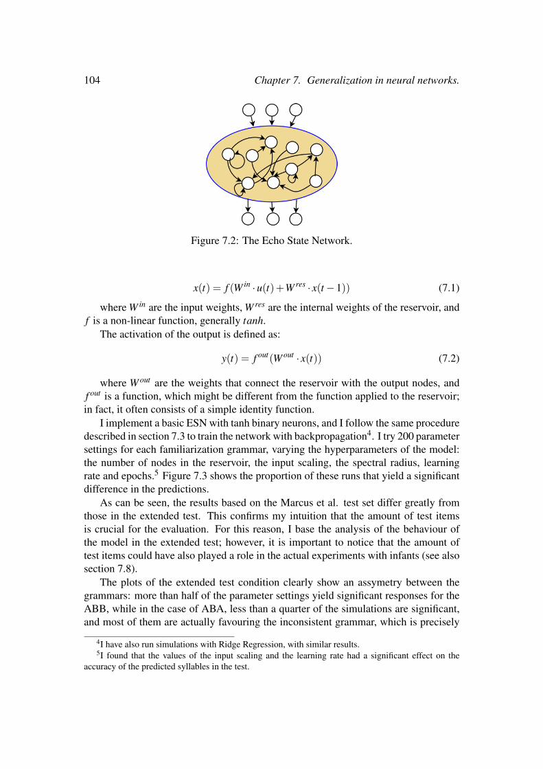
104 Chapter 7. Generalization in neural networks.
Figure 7.2: The Echo State Network.
x(t) = f (W in ·u(t)+W res · x(t−1)) (7.1)
where W in are the input weights, W res are the internal weights of the reservoir, andf is a non-linear function, generally tanh.
The activation of the output is defined as:
y(t) = f out(W out · x(t)) (7.2)
where W out are the weights that connect the reservoir with the output nodes, andf out is a function, which might be different from the function applied to the reservoir;in fact, it often consists of a simple identity function.
I implement a basic ESN with tanh binary neurons, and I follow the same proceduredescribed in section 7.3 to train the network with backpropagation4. I try 200 parametersettings for each familiarization grammar, varying the hyperparameters of the model:the number of nodes in the reservoir, the input scaling, the spectral radius, learningrate and epochs.5 Figure 7.3 shows the proportion of these runs that yield a significantdifference in the predictions.
As can be seen, the results based on the Marcus et al. test set differ greatly fromthose in the extended test. This confirms my intuition that the amount of test itemsis crucial for the evaluation. For this reason, I base the analysis of the behaviour ofthe model in the extended test; however, it is important to notice that the amount oftest items could have also played a role in the actual experiments with infants (see alsosection 7.8).
The plots of the extended test condition clearly show an assymetry between thegrammars: more than half of the parameter settings yield significant responses for theABB, while in the case of ABA, less than a quarter of the simulations are significant,and most of them are actually favouring the inconsistent grammar, which is precisely
4I have also run simulations with Ridge Regression, with similar results.5I found that the values of the input scaling and the learning rate had a significant effect on the
accuracy of the predicted syllables in the test.

7.5. Pre-Wiring: Delay Line Memory 105
ABA
6.50%1.00%
92.50%
Extended test.ABA
1.50%
21.50%
77.00%
ABB
7.00%
8.00%
85.00%
Extended test.ABB
60.50%
0.00%
39.50%
Sign. Cons. Sign. Incons. Not Sign.
Figure 7.3: Proportion of parameter settings that yield significant (white), non-significant (dark grey) and inconsistently significant (light grey) responses, for thesimulation with the basic ESN.
ABB. As mentioned before, the reason for this assymetry is probably due to the factthat immediate repetitions are easier to learn, since they are less affected from thedecay of the activation function; for now, it suffices to say that the behaviour of themodel towards ABA does not suggest that it could be a potential explanation for theexperimental results.
7.5 Pre-Wiring: Delay Line MemoryIn order to succeed in the prediction task, the model must predict a syllable that isidentical to one presented before. In the previous simulations, I relied on the mem-ory that ESNs offer through the recurrent connections and the Echo Property [Jaeger,2002]. However, there exist several computational alternatives that brains may use toimplement memory [Chaudhuri and Fiete, 2016]. I now explore one such model ofmemory: a delay line.
Figure 7.4: Depiction of five timesteps in the DeLi-ESN. The highlighted nodes showthe activations in the delay line (the activation of the rest of the nodes is not illustrated).

106 Chapter 7. Generalization in neural networks.
Computationally, a delay line is a mechanism that ensures the preservation of theinput by propagating it in a path (“line”) that implements a delay. In the brain, delaylines have been proposed as part of the sound localization system [Jeffress, 1948], andthey have been identified through intracellular recordings in the barn owl brain [Carrand Konishi, 1988]. In a neural network, a delay line is naturally implemented byorganizing a subnetwork of neurons in layers, with “copy connections” (with weights1 between corresponding nodes and 0 everywhere else) connecting each layer to thenext. In this way, the information is kept in the network for as many timesteps asdedicated layers in the network (see figure 7.4).
I implement a delay line memory in the ESN (creating thus a new model that I callDeLi-ESN) by imposing this layer structure in the reservoir. I run 1200 combinationsof parameter settings with the DeLi-ESN, including also a parameter that establishessome amount of noise to add to the weights of the reservoir. In this way, some modelscontain a less strict delay line; the greater the noise, the closer the model is to theoriginal ESN.
ABA
5.83%0.17%
94.00%
Extended test.ABA
11.33%
5.67%
83.00%
ABB
3.33%
18.00%
78.67%
Extended test.ABB
57.50%
0.17%
42.33%
Sign. Cons. Sign. Incons. Not Sign.
Figure 7.5: Proportion of parameter settings that yield significant, non-significant andinconsistently significant responses in the tests, for the simulation with DeLi-ESN.
The results, illustrated in Figure 7.5, show an increased number of significant re-sponses (in favour of the consistent grammar) for the extended test of ABA familiariza-tion: the addition of the delay line memory indeed helps in the detection of the identityrelation. But in spite of the positive effect of the delay line, we need to ask ourselvesto what extent these results are satisfactory. The pie plots show the likelihood of ob-taining with my model the results that Marcus et al. found in their experiments, andin order to do so, I use the same measure of success (i.e. whether the responses foreach grammar are significantly different). However, the models hardly ever producethe correct prediction6. For this reason, in the next section, I adopt a stricter measure
6I find that the values of the input scaling, learning rate, spectral radius, reservoir size, and reservoirnoise each have a significant effect on the accuracy of the predicted syllables in the test, although exact

7.6. Pre-Training: Incremental-Novelty Exposure 107
of success. I discuss this issue further in section 7.8.
7.6 Pre-Training: Incremental-Novelty ExposureThe infants that participated in the original experiment had surely been exposed to hu-man speech before the actual experiment; however, in most computational simulationsthis fact is obviated. I hypothesize that prior perceptual experience could have trig-gered a bias for learning abstract solutions: since the environment is variable, infantsmay have adapted their induction mechanism to account for novel instances. I nowpropose a method to pre-train a neural network that aims to incorporate this intuition.
In this training regime —which I call Incremental-Novelty Exposure, or INE forshort— I iteratively train and test my model; so for a certain number of iterations i, themodel is trained and tested i times, with the parameters learnt in one iteration being theinitial state of the next iteration. The test remains constant in each of these iterations;however, the training data is slightly modified from one iteration to the next. The firsttraining set is designed according to the Marcus et al. stimuli: 4 syllables of type Aand 4 syllables of type B are combined according to the pattern of the familiarizationgrammar (ABA or ABB). In the second iteration, one syllable of type A and one oftype B are deleted (that is, all the triplets involving those syllables are removed fromthe training set), and a new syllable of type A and one of type B are incorporated, suchthat new triplets of the familiarization pattern are generated with the new syllables(combined as well with the already-present syllables). Therefore, for each trainingiteration, the model is exposed to a similar training set as the previous iteration, butthere is a small amount of novelty. This procedure is illustrated in figure 7.6.
I simulate 600 different hyperparameter configurations, varying the reservoir size,noise in the delay line, input scaling, spectral radius, learning rate, and epochs. Figure7.7 illustrates how the mean accuracy evolves at each stage of the INE procedure ofone representative run. As it can be seen in the graphs, the accuracy is really lowin the beginning (corresponding to a simulation without pre-training) but, with moreiterations –and thus with more novel items incorporated in the training set–, the modelbecomes better, presumably by finding a more general solution.
In order to test that these results are robust, I compute the mean over the accuracyfor the last quarter of the tests (in this case, the last 25 tests, corresponding to the right-most curve in the graph), for a few runs. The results are fairly similar in each run, ascan be seen in figure 7.8a. Thus, the combination of the DeLi-ESN and the INE dras-tically boosts the generalization capabilities of the ESN; however, we should identifywhat is the contribution of the DeLi-ESN. Figure 7.8b shows the mean accuracy (again,for the last quarter of the regime), for 16 runs of the basic ESN in the INE regime. Theeffect of the delay line memory is clear: when removed, the accuracy is close to 0 forABA, and mostly around 20% for ABB.
prediction accuracy remains low (rarely above 12% for ABA and above 20% for ABB familiarization)even for the best combination of parameters.

108 Chapter 7. Generalization in neural networks.
Figure 7.6: Depiction of the Incremental-Novelty Exposure. Barred syllables are re-moved from the training set after the training of the corresponding iteration has finished(so they do not remain in the training set of the next iteration).
7.7 Discussion: Relation with other neural network tech-niques
The task defined by Marcus and colleagues is simple, but the difficulty it presents forneural networks has been taken to reveal a fundamental limitation of such networks inreal world tasks. I now therefore briefly discuss how my solution to these difficultiesmight relate to other methods in artificial intelligence and deep learning.
7.7.1 Relation with Recurrent Neural Networks
My model differs from the SRN model, and from Recurrent Neural Network (RNN)more generally, in its adoption of the reservoir computing approach. Concretely thismeans the weights from the input layer to the hidden layer, and the recurrent weightsfrom the hidden layer to itself, are never updated. Thus, learning only occurs in theoutput layer.
This has important consequences for how each model implements a memory. InRNNs, input from previous time steps may continue to play a role through the re-current connections. Since those connections are updated during training, the modelmust learn what to memorize and how to combine it with novel input. In contrast, inreservoir computing models, the reservoir is designed, by enforcing the echo property,to have informations from past inputs (and initialization) linger around in the recur-rent connections (and this information is asymptotically ’washed out’ [Jaeger, 2007]).Hence, the architecture does not need to learn to memorize information, but rather mayfocus on how to use both the memorized and current input to solve a task.
There is an interesting connection between the echo state property in reservoir com-

7.7. Discussion: Relation with other neural network techniques 109
Figure 7.7: Performance over 100 iterations with Incremental Novelty Exposure, forone representative run in the ABA familiarization condition (left) and one in the ABBcondition (right).
puting and the now popular ‘orthogonal initialization’ for recurrent networks. In echostate networks, the echo state property is often achieved by ensuring, as I do in here,that the spectral radius (largest eigen value) of the recurrent weight matrix has a valuejust below 1.0 (although this is neither a sufficient nor a necessary condition for theecho state property to hold; see Jaeger 2007). In ‘orthogonal initialization’ all eigen-values of that matrix have an absolute value of 1; the largest eigenvalues will thusinitially be 1.0, before backpropagation gradually changes the weights and eigen val-ues.
7.7.2 Relation with standard Echo State NetworkThere are two main changes in my model that deviate from the standard ESN. Firstof all, by pre-wiring the reservoir, I depart from the original implementation, in whichthe reservoir is randomly initialized (although constrained to satisfy the echo stateproperty). This has an effect on the type of memory the model has access to. Instandard ESN’s, the echo state property ensures that the information of previous inputlingers around, but not that this information remains represented in the same way: any(sub)vector representing the information of interest at time t might be inverted, rotatedor projected into another subspace at any time t. Instead, the delay line in my modelkeeps information in the same representation (and projected to a dedicated subspacefor each time delay).
Another aspect that deviates from common implementations of ESN is that I trainthrough gradient descent, while generally, ESNs are trained with Ridge Linear Regres-sion. The latter is a simple and fast solution, works over a convex error function, andconverges to the global optimum. However, for the ’Incremental Novelty Exposure’in section 7.6, the global optimum for the current training set is not what is lookedfor. Key to the success of that approach is that previous training phases still have an

110 Chapter 7. Generalization in neural networks.
(a) DeLi-ESN
(b) Basic ESN
Figure 7.8: Mean accuracy for the tests in the last quarter simulation in the INE simu-lation, for DeLi-ESN (a) and basic ESN (b).
effect on the current. With my use of stochastic gradient descent, my model exploresmultiple local optima, and thus has a chance to find a solution that generalizes beyondthe current datasets.
7.7.3 Pre-Wiring: Relation with LSTMs
The incorporation of a Delay Line extends the memory of the model in a particular way,by forcing the persistence of an explicit representation of the input for a certain time.This technique relates to Long Short Term Memory (LSTM) networks Hochreiter andSchmidhuber [1997], a variant of RNNs that also augments recurrent networks with a’memory cell’.
In LSTMs, the hidden layer is extended to incorporate a circuitry of gates thatcontrol the flow of information. The core of such circuitry is the memory cell, thecomponent that maintains a persistent copy of the input over time. The gates add or

7.8. Conclusion 111
remove information from the cell state through linear operations. Thus, the gates aredesigned to learn which information should be forgotten or retrieved, while the statecell acts like a conveyor belt on which the input is propagated over time.
Both the delay line and the gated memory in LSTMS are incorporated to the net-works to ensure persistence of the input by copying it over timesteps. However, thetechniques also exhibit notable differences in how the information is propagated: whilein LSTMs, the information in the cell state is only modified with linear operations, thedelay line incorporates a non-linear activation function (tanh) that has the effect of ap-plying a form of decay over the input, such that the input values are closer to zero afterevery timestep.
These models also exhibit a different approach to forgetting. As mentioned, mymodel incorporates some form of forgetting by decaying the input over time. This de-cay is applied uniformly to all the units participating in the representation of a certaininput vector. In contrast, in LSTMs the information does not uniformly and constantlydeteriorate over time. Instead, the gate circuitry incorporates a forget gate that is trainedto decide which information of the cell state should decay or be removed. The gate op-erates over units rather than over vectors, so the features of the input are not uniformlysurpressed.
7.7.4 Pre-training: Relation with DropoutThe Incremental Novelty Exposure training regime of section 7.6, also finds a counter-part in the current deep learning literature, in the regularization technique of Dropout(Hinton et al. 2012, Srivastava et al. 2014). The idea behind Dropout is that, by ran-domly removing some of the units of the network during training, the model is forcedto find solutions that do not rely too much on concrete correlations. This intuition issimilar to the one that guides the INE: by constantly adding some novelty to the data,I force the network to not rely too much on accidental correlations. The crucial differ-ence between both techniques is that Dropout modifies the architecture of the networkto achieve this purpose, while the INE achieves a similar effect by manipulating thetraining data.
7.8 ConclusionThe Marcus et al. publication conveyed two main statements: first, that infants spon-taneously extract identity rules from a short familiarization, and second, that neuralnetworks are doomed to fail in such simple task. My work suggests that both the initialoptimism for the generalization abilities of infants and the pessimism towards neuralnetworks were overstated.
This study investigates the initial conditions that a neural network model shouldimplement in order to account for the experimental results. First, I have proposed thatnetworks should be pre-wired to incorporate a bias towards memorization of the input,

112 Chapter 7. Generalization in neural networks.
which I have implemented as a delay line. With such pre-wiring, the model yields anotable proportion of significantly different responses between grammars. But despitesuch apparent success, the accuracy of the model in syllable prediction is very low.
Therefore, even though the successful discrimination between grammars is gener-ally understood as abstraction of the underlying rule, my results show that significantlydifferent responses can easily be found in a model that has not perfectly learnt such arule. The corollary is that the generalization abilities of infants may have been overesti-mated; as a matter of fact, null results in similar experiments also point in that direction(see for instance footnote 1 in Gerken [2006]; also Geambasu&Levelt, p.c.).
But can neural networks go beyond grammar discrimination and accurately predictthe next syllable according to a generalized rule? This work shows that this can beachieved when prior experience is incorporated in the model. I have hypothesizedthat, from all the information available in the environment, it is the gradual exposureto novel items that enhances generalization. This particular hypothesis deviates fromrelated studies in which (i) an SRN was pre-trained to learn the relation of samenessbetween syllables [Seidenberg and Elman, 1999a], and (ii) an SRN was pre-trainedwith a set of sentences generated from a uniformly sampled vocabulary. Although thedata used in the pre-training proposed here is less realistic than that used by Altmann[2002], my evaluation method is more strict (since I aim to test for accuracy rather thandiscrimination); for this reason, I first need to evaluate a model with a more constrainedinput. The next step in future work should be to explore whether the same results canbe obtained when input data involving gradual novelty is generated from a grammarunrelated to the actual experiment.
Finally, from the perspective of the symbol vs. associations debate, at some ab-stract level of description, the delay line may be interpreted as providing the modelwith variables (that is, the dedicated group of nodes that encode the input at a certaintime may be seen as a register) and the symbolic operation of “copy”. It should benoted though that these groups of nodes are not isolated, and therefore, the learningalgorithm needs to discover the structure in order to make use of it. Furthermore, itis uncontroversial that items are kept in memory for a certain lapse of time, so thisstructure is unlikely to constitute the core of the symbolic enterprise. If neverthelessmy model is seen as compatible with the theory of rules-over-variables, my approachmay be seen as providing a unifying model in which both sides in the debate can seetheir proposals reflected.

Conclusions
113


Chapter 8
Conclusions
8.1 Summary
The goal of this dissertation was to use the methodology offered by computationalmodelling to advance the current knowledge on the cognitive mechanisms behind ALLexperiments. In my approach to the challenge, I conceptualized the process of learningthe basic rules of a language as consisting of three steps: (i) memorization of sequencesegments, (ii) computing the propensity to generalize, and (iii) generalization. In thisdissertation I have proposed an account of each of these steps with a computationalmodel.
Step (i) is relevant to understand how individuals segment a speech stream. Inchapter 3 I have proposed R&R, a processing model that explains segmentation as aresult of retention and recognition. This model offered an intuitive explanation of theprocess, and prompted the discovery that the memorization of segments tends to followa skewed distribution rather than one that clearly separates statistically coherent items(words) from other segments of similar length but less statistically salient (partwords).
For step (ii), I propose that Simple Good Turing [Good, 1953], an existing smooth-ing model used in Natural Language Processing to account for unseen words in cor-pora, can be taken as a rational model. The principle it is based on —that the numberof useful unseen items can be estimated from the number of times that items are seenonce, twice, thrice, etc.— can explain the responses of individuals in the experiments.
As for step (iii), I first presented an extensive critical review of the existing mod-els (chapter 6), in order to assess the state of the art and the critical issues that havenot been resolved yet. After listing a desiderata for future research on generalization,I present a neural network model that emphasizes the role of the initial state of themodel, based on two core ideas: pre-wiring the connections of the network to provideit with another type of memory, and pre-training to account for the relevant experi-ence that influences generalization (concretely, experience that gradually incorporatesnovelty).
115

116 Chapter 8. Conclusions
8.2 Contributions I: Exploring better ways to evaluatemodels
As reflected in § 2.4, there are no a priori criteria to determine what constitutes agood model. In this dissertation I have employed and developed different forms ofevaluation.
To begin with, in chapter 5 I use model sequencing to study the behavior of modelswhen combined in a pipeline sequence –that is, the output of one model (in this case theoutput of the R&R model) is used as the input of the next model (SGT). As reported,thanks to the contribution of both models the final output coincides with the empiricaldata.
In chapter 4 I used model parallelisation instead, to compare a range of modelsbased on their goodness of fit to data from a number of experiments. As reported inthat chapter, also for model parallelisation we can find different types of evaluation,roughly divided on those that assess the internal representations built by models whileprocessing the stimuli, or those based instead on the ‘behavioural responses’ of themodel. These are complementary forms of evaluation, but as shown, evaluation basedon certain aspects of internal representations (in this case frequency distributions) canbe necessary to differentiate between models.
Finally, in chapter 7 I evaluated my model based on two criteria: whether the modelproduced ‘responses’ that are sufficiently different between conditions, or whether itpredicted the ‘correct’ outcome. The former was applied with the aim of reproducingthe empirical results, while the latter aimed to assess the accuracy of the model, in orderto address a more general theoretical question about whether perfect generalization inthis model can be achieved.
After exploring these various forms of evaluation, what becomes clear is that eachstudy may require a different approach, but in all cases modellers should strive tobe very strict and creative in defining evaluation criteria that challenges models suffi-ciently to be able to distinguish between alternative models.
8.3 Contributions II: Exploring complementary levelsof analysis
The models proposed throughout this dissertation are pitched at different levels of anal-ysis. As advanced in chapter 2, each level suits different objectives.
To begin with, R&R is a processing level model. The main reason for this choiceis that, in segmentation, the key open questions are about differences in behaviourbetween age groups and species. These differences cannot be investigated with rationalmodels, since those models do not incorporate any properties of the cognitive system.Likewise, addressing these questions at the neural level is not likely to be helpful, sincewe require interpretable theories before addressing which implementational properties

8.4. Contributions III: Reframing key theoretical debates 117
are responsible for the observed differences. And indeed, after proposing this modelwe have an intuitive theory of segmentation, based on basic perceptual and memoryprocesses of retention and recognition.
In generalization, I identified a misconception in the field: namely, that statisticalmodels should always generalize more when presented with more data. I have used arational model (SGT, [Good, 1953]) to show that, when accounting for the propensityto generalize, this premise turns out to be false. This approach served as a first step toconceptualize the problem, and it paves the way for future models at the processing orimplementational level.
Finally, I have proposed an implementational model of generalization (chapter 7).The goal of this model was precisely to understand how behaviour that appears sym-bolic can be accounted for at the implementational level, without the use of rules andsymbols; hence this level of analysis was called for. Additionally, as seen in the corre-sponding chapter, the symbolic models proposed to explain the experiment in Marcuset al. [1999] are very simple: when assuming predefined rules over existing variables,the models do not offer much room for unexpected findings or predictions.
These three models target different types of questions, and it has been clearly usefulto adhere to different levels of analysis depending on each particular goal.
8.4 Contributions III: Reframing key theoretical debates
One of the main advantages of the computational modelling methodology is that itforces researchers to be precise about all the details in a theory, and hence it helps clar-ifying misunderstandings. There are two important debates to which this dissertationhas contributed.
First of all, with the proposal of a model for the propensity to generalize (chapter5), I contributed to the debate about one vs. multiple mechanisms. Roughly speaking,most ALL studies can be categorized in one of these positions: those that postulate thatthe same mechanism for segmentation can be extended to account for generalization,and those which argue that we need to postulate an additional mechanism of a differentnature. With my work, I have shown that one of the arguments for the latter position—namely, that a single statistical mechanism would predict better generalization withlonger exposure— was a result of lack of formalization; a simple rational model likeSimple Good Turing sufficed to illustrate this point.
Second, I have also contributed to a prominent debate about the allegedly sym-bolic nature of the mechanism of generalization. As reviewed in chapter 6, the debatecondenses in disagreement on the cognitive realism of rules and variables (although Iidentified other questions to which computational models can contribute). The neuralnetwork model proposed in chapter 7 shows that a non-symbolic model can learn touse the information in a way that is descriptively equivalent to the use of rules overvariables, even though at the level of implementation there are no rules or variables.

118 Chapter 8. Conclusions
8.5 Future workThis dissertation has been structured along the three-step approach, which is a high-level conceptualization of the learning processes that take place in ALL experiments.Even though I have proposed a model for each step, there are details about the wholeapproach that are still underspecifed.
For instance, does the flow of information always proceed as a pipeline, or are steps(ii) and (iii) being constantly updated while step (i) is taking place? This may appearirrelevant if the information flows unidirectionaly, but we do not know if that is actuallythe case. For instance, the generalizations derived in step (iii) may have an influenceon what is being memorized in step (i). These are open questions that this dissertationdoes not address and thus they should be tackled in future work.
Likewise, a more integrated model of the three steps is missing: while in chapter5 I have used model sequencing to show that the output of step (i) has the necessaryproperties for step (ii) to reproduce the empirical data, this type of serialization ismissing for connecting steps (ii) and (iii). Although the conceptualization makes itclear that the propensity to generalize is quantified as a probability for unseen itemsthat should be divided between the generalized items computed in step (iii), how thisprobability is actually divided among these items has not been formalized yet.
Another direction that should be further explored is to extend the cross-speciesanalysis with other animal species. In chapter 3 I presented simulations based onALL experiments with rats, but as mentioned in the introduction (chapter 1), thereexists a large body of ALL experiments involving other animals, such as birds andprimates. These experiments are often not directly comparable with those on humans(e.g. experiments with songbirds generally require extensive training with feedback,and this contrasts especially with human infant experiments in which learning is typ-ically spontaneous after short familiarization), but computational simulations may beused in creative ways to investigate empirical results in different species.
Finally, even in the case of humans, the datasets that have been studied in thisdissertation are relatively small. This limitation is most serious in the case of general-ization (step (iii)), for which I have focused exclusively on the data from Marcus et al.[1999] despite the existence of other experiments (see chapter 1 for other examples ofgeneralization experiments in ALL). The reason for this is that the Marcus et al. exper-iment offers a very clean and illustrative dataset, and in spite of the replication issues,it is conceptually useful to discuss the challenges of generalization. Nonetheless, thepredictions of models of generalization should be tested against other existing datasetsto move forward on this question.

Bibliography
K. Abe and D. Watanabe. Songbirds possess the spontaneous ability to discriminatesyntactic rules. Nature neuroscience, 14(8):1067–1074, 2011.
R. G. Alhama and W. Zuidema. Generalization in artificial language learning: Mod-elling the propensity to generalize. Proceedings of the 7th Workshop on Cog-nitive Aspects of Computational Language Learning, pages 64–72, 2016. URLhttp://anthology.aclweb.org/W16-1909.
R. G. Alhama and W. Zuidema. Pre-wiring and pre-training: What does a neuralnetwork need to learn truly general identity rules? Under review, 2017a.
R. G. Alhama and W. Zuidema. Segmentation as retention and recognition: the R&Rmodel. Proceedings of the 39th Annual Conference of the Cognitive Science Society.,2017b.
R. G. Alhama and W. Zuidema. Computational models of rule learning. To be submit-ted., 2017c.
R. G. Alhama, R. Scha, and W. Zuidema. Rule Learning in Humans and Animals,chapter 49, pages 371–372. 2014.
R. G. Alhama, R. Scha, and W. Zuidema. How should we evaluate models of segmenta-tion in artificial language learning? In Proceedings of 13th International Conferenceon Cognitive Modeling, 2015.
R. G. Alhama, R. Scha, and W. Zuidema. Memorization of sequence-segments byhumans and non-human animals: the Retention-Recognition model. ILLC Prepub-lications, PP-2016-08, 2016.
A. Alishahi and S. Stevenson. A computational model of early argument structureacquisition. Cognitive Science, 32(5):789–834, 2008.
119
120 BIBLIOGRAPHY
G. T. Altmann. Learning and development in neural networks–the importance of priorexperience. Cognition, 85(2):B43–B50, 2002.
G. T. Altmann and Z. Dienes. Rule learning by seven-month-old infants and neuralnetworks. Science, 284(5416):875–875, 1999.
J. R. Anderson. Rules of the mind. Psychology Press, 2014.
R. N. Aslin, J. R. Saffran, and E. L. Newport. Computation of conditional probabilitystatistics by 8-month-old infants. Psychological science, 9(4):321–324, 1998.
C. Bannard, E. Lieven, and M. Tomasello. Modeling children’s early grammaticalknowledge. Proceedings of the National Academy of Sciences, 106(41):17284, 2009.
J. Batali. The negotiation and acquisition of recursive grammars as a result of com-petition among exemplars. In Linguistic evolution through language acquisition:Formal and computational models. Citeseer, 1999.
G. J. Beckers, J. J. Bolhuis, K. Okanoya, and R. C. Berwick. Birdsong neurolinguistics:Songbird context-free grammar claim is premature. Neuroreport, 23(3):139–145,2012.
R. Bod. Exemplar-based syntax: How to get productivity from examples. The linguisticreview, 23(3):291–320, 2006.
G. Borensztajn, W. Zuidema, and R. Bod. Children’s grammars grow more abstractwith age—evidence from an automatic procedure for identifying the productive unitsof language. Topics in Cognitive Science, 1(1):175–188, 2009.
J. S. Bowers. On the biological plausibility of grandmother cells: implications forneural network theories in psychology and neuroscience. Psychological review, 116(1):220, 2009.
J. S. Bowers. More on grandmother cells and the biological implausibility of PDPmodels of cognition: A reply to Plaut and McClelland (2010) and Quian Quirogaand Kreiman (2010). Psychological Review, 2010.
C. E. Carr and M. Konishi. Axonal delay lines for time measurement in the owl’sbrainstem. Proceedings of the National Academy of Sciences, 85(21):8311–8315,1988.
N. Chater and P. Vitanyi. Simplicity: a unifying principle in cognitive science? Trendsin Cognitive Sciences, 7(1):19 – 22, 2003. ISSN 1364-6613. doi: http://dx.doi.org/10.1016/S1364-6613(02)00005-0. URL http://www.sciencedirect.com/science/article/pii/S1364661302000050.

BIBLIOGRAPHY 121
R. Chaudhuri and I. Fiete. Computational principles of memory. Nature neuroscience,19(3):394–403, 2016.
N. Chomsky. Syntactic Structures. Mouton, The Hague, 1957.
N. Chomsky. Aspects of the Theory of Syntax, volume 119. MIT Press (MA), 1965.
N. Chomsky. Rules and representations. Behavioral and Brain Sciences, 3(01):1–15,1980.
N. Chomsky. Knowledge of language: Its nature, origin, and use. Greenwood Pub-lishing Group, 1986.
M. Christiansen, C. Conway, and S. Curtin. A connectionist single mechanism accountof rule-like behavior in infancy. In Proceedings of the 22nd annual conference ofthe cognitive science society, pages 83–88, 2000.
M. H. Christiansen and S. Curtin. Transfer of learning: rule acquisition or sta-tistical learning? Trends in Cognitive Sciences, 3(8):289 – 290, 1999. ISSN1364-6613. doi: http://dx.doi.org/10.1016/S1364-6613(99)01356-X. URL http://www.sciencedirect.com/science/article/pii/S136466139901356X.
M. H. Christiansen, J. Allen, and M. S. Seidenberg. Learning to segment speech usingmultiple cues: A connectionist model. Language and cognitive processes, 13(2-3):221–268, 1998.
A. Clark and S. Lappin. Linguistic Nativism and the Poverty of the Stimulus. JohnWiley & Sons, 2010.
E. V. Clark. First language acquisition. Cambridge University Press, 2009.
A. Cleeremans and J. L. McClelland. Learning the structure of event sequences. Jour-nal of Experimental Psychology: General, 120(3):235, 1991.
F. Crick. The recent excitement about neural networks. Nature, 337:129–132, 1989.
W. Croft. Radical construction grammar: Syntactic theory in typological perspective.Oxford University Press, USA, 2001.
W. Daelemans, S. Gillis, and G. Durieux. The acquisition of stress: A data-orientedapproach. Computational Linguistics, 20(3):421–451, 1994.
Z. Dienes, G. Altmann, and S.-J. Gao. Mapping across domains without feedback: Aneural network model of transfer of implicit knowledge. Cognitive Science, 23(1):53–82, 1999.
122 BIBLIOGRAPHY
P. F. Dominey. Complex sensory-motor sequence learning based on recurrent staterepresentation and reinforcement learning. Biological cybernetics, 73(3):265–274,1995.
P. F. Dominey and F. Ramus. Neural network processing of natural language: I. sensi-tivity to serial, temporal and abstract structure of language in the infant. Languageand Cognitive Processes, 15(1):87–127, 2000.
P. Eimas. Do infants learn grammar with algebra or statistics? Science, 284(5413):435, 1999.
J. Elman. Generalization, rules, and neural networks: A simulation of marcus et. al.(1999). Html document., 1999.
J. L. Elman. Finding structure in time. Cognitive Science, 14(2):179–211, 1990.
J. L. Elman. Rethinking innateness: A connectionist perspective on development, vol-ume 10. MIT press, 1998.
A. Endress and L. Bonatti. Rapid learning of syllable classes from a perceptuallycontinuous speech stream. Cognition, 105(2):247–299, 2007.
A. Endress and L. Bonatti. Words, rules, and mechanisms of language acquisition.WIREs Cognitive Science, 2016. (in press).
A. Endress, G. Dehaene-Lambertz, and J. Mehler. Perceptual constraints and the learn-ability of simple grammars. Cognition, 105(3):577–614, 2007.
A. D. Endress. Bayesian learning and the psychology of rule induction. Cognition,127(2):159–176, 2013.
A. D. Endress, B. J. Scholl, and J. Mehler. The role of salience in the extraction ofalgebraic rules. Journal of Experimental Psychology: General, 134(3):406, 2005.
S. E. Fahlman and C. Lebiere. The cascade-correlation learning architecture. Advancesin Neural Information Processing Systems 2, pages 524–532, 1990.
C. J. Fillmore, P. Kay, and M. C. O’connor. Regularity and idiomaticity in grammaticalconstructions: The case of let alone. Language, pages 501–538, 1988.
W. T. Fitch and M. D. Hauser. Computational constraints on syntactic processing in anonhuman primate. Science, 303(5656):377–380, 2004.
J. A. Fodor and Z. W. Pylyshyn. Connectionism and cognitive architecture: A criticalanalysis. Cognition, 28(1):3–71, 1988.
M. Frank and J. Tenenbaum. Three ideal observer models for rule learning in simplelanguages. Cognition, 120(3):360–371, 2011.

BIBLIOGRAPHY 123
M. C. Frank. Throwing out the bayesian baby with the optimal bathwater: Responseto Endress (2013). Cognition, 128(3):417 – 423, 2013.
M. C. Frank, S. Goldwater, T. L. Griffiths, and J. B. Tenenbaum. Modeling humanperformance in statistical word segmentation. Cognition, 2010.
S. L. Frank and M. Cernansky. Generalization and systematicity in echo state net-works. In . V. S. B.C. Love, K. McRae, editor, Proceedings of the 30th AnnualConference of the Cognitive Science Society, pages 733–738. Cognitive Science So-ciety, 2008.
R. M. French and G. W. Cottrell. Tracx 2.0: A memory-based, biologically-plausiblemodel of sequence segmentation and chunk extraction. In Proceedings of the 36thAnnual Conference of the Cognitive Science Society, 2014.
R. M. French, C. Addyman, and D. Mareschal. Tracx: A recognition-based connec-tionist framework for sequence segmentation and chunk extraction. PsychologicalReview, 118(4):614, 2011.
R. L. Frost and P. Monaghan. Simultaneous segmentation and generalisation of non-adjacent dependencies from continuous speech. Cognition, 147:70–74, 2016.
W. Gale and G. Sampson. Good-turing frequency estimation without tears. Journal ofQuantitative Linguistics, 2(3):217–237, 1995.
L. Gamut. Logic, Language, and Meaning: Intensional logic and logical grammar.University of Chicago Press, 1991.
M. Gasser and E. Colunga. Babies, variables, and relational correlations. In Pro-ceedings of the Twenty-second Annual Conference of the Cognitive Science Society:August 13-15, 2000, Institute for Research in Cognitive Science, University of Penn-sylvania, Philadelphia, PA, volume 22, page 160. Lawrence Erlbaum Associates,2000.
W. S. Geisler. Ideal observer analysis. The visual neurosciences, pages 825–837, 2003.
T. Gentner, K. Fenn, D. Margoliash, and H. Nusbaum. Recursive syntactic patternlearning by songbirds. Nature, 440(7088):1204–1207, 2006.
L. Gerken. Decisions, decisions: infant language learning when multiple generaliza-tions are possible. Cognition, 98(3):B67 – B74, 2006. ISSN 0010-0277.
E. M. Gold. Language identification in the limit. Information and control, 10(5):447–474, 1967.
A. Goldberg. Constructions: A construction grammar approach to argument structure.University of Chicago Press, 1995.
124 BIBLIOGRAPHY
S. Goldwater, T. L. Griffiths, and M. Johnson. Contextual dependencies in unsuper-vised word segmentation. In Proceedings of the annual meeting of the associationfor computational linguistics, volume 44, pages 673–680, 2006.
S. Goldwater, T. L. Griffiths, and M. Johnson. A bayesian framework for word seg-mentation: Exploring the effects of context. Cognition, 112:21–54, 2009.
R. L. Gomez. Variability and detection of invariant structure. Psychological Science,13(5):431–436, 2002.
R. L. Gomez and L. Gerken. Artificial grammar learning by 1-year-olds leads to spe-cific and abstract knowledge. Cognition, 70(2):109–135, 1999.
I. J. Good. The population frequencies of species and the estimation of populationparameters. Biometrika, 40(3-4):237–264, 1953.
A. Graves, G. Wayne, and I. Danihelka. Neural turing machines. arXiv preprintarXiv:1410.5401, 2014.
T. L. Griffiths, N. Chater, C. Kemp, A. Perfors, and J. B. Tenenbaum. Probabilis-tic models of cognition: exploring representations and inductive biases. Trends incognitive sciences, 14(8):357–364, 2010.
R. Gomez and J. Maye. The developmental trajectory of nonadjacent dependencylearning. Infancy, 7(2):183–206, 2005. ISSN 1532-7078.
M. D. Hauser, E. L. Newport, and R. N. Aslin. Segmentation of the speech stream ina non-human primate: Statistical learning in cotton-top tamarins. Cognition, 78(3):B53–B64, 2001.
D. O. Hebb. The organization of behavior: A neuropsychological theory. John Wiley& Sons, 1949.
G. E. Hinton, N. Srivastava, A. Krizhevsky, I. Sutskever, and R. R. Salakhutdinov.Improving neural networks by preventing co-adaptation of feature detectors. arXivpreprint arXiv:1207.0580, 2012.
S. Hochreiter and J. Schmidhuber. Long short-term memory. Neural computation, 9(8):1735–1780, 1997.
J. J. Hopfield. Neurons with graded response have collective computational propertieslike those of two-state neurons. Proceedings of the national academy of sciences,81(10):3088–3092, 1984.
J. E. Hummel. Getting symbols out of a neural architecture. Connection Science, 23(2):109–118, 2011.

BIBLIOGRAPHY 125
R. Jackendoff. Foundations of language: brain, meaning, grammar, evolution. Oxford:Oxford University Press, 2003.
H. Jaeger. The ‘‘echo state’’ approach to analysing and training recurrent neural net-works. Technical report, German National Research Center for Information Tech-nology, 2001.
H. Jaeger. Short term memory in echo state networks. Technical report, GermanNational Research Center for Information Technology, 2002.
H. Jaeger. Echo state network. Scholarpedia, 2(9):2330, 2007.
L. A. Jeffress. A place theory of sound localization. Journal of comparative andphysiological psychology, 41(1):35, 1948.
M. F. Joanisse and J. L. McClelland. Connectionist perspectives on language learning,representation and processing. Wiley Interdisciplinary Reviews: Cognitive Science,6(3):235–247, 2015.
E. Keuleers and W. Daelemans. Memory-based learning models of inflectional mor-phology: A methodological case-study. Lingue e linguaggio, 6(2):151–174, 2007.
S. Kirby, M. Dowman, and T. L. Griffiths. Innateness and culture in the evolution oflanguage. Proceedings of the National Academy of Sciences, 104(12):5241–5245,2007. doi: 10.1073/pnas.0608222104. URL http://www.pnas.org/content/104/12/5241.abstract.
D. C. Knill and A. Pouget. The bayesian brain: the role of uncertainty in neural codingand computation. Trends in neurosciences, 27(12):712–719, 2004.
S. E. Kuehne, D. Gentner, and K. D. Forbus. Modeling infant learning via symbolicstructural alignment. In Proceedings of the twenty-second annual conference of thecognitive science society, pages 286–291, 2000.
C. Kurumada, S. C. Meylan, and M. C. Frank. Zipfian frequency distributions facilitateword segmentation in context. Cognition, 127(3):439–453, 2013.
M. D. Lee and E.-J. Wagenmakers. Bayesian cognitive modeling: A practical course.Cambridge University Press, 2014.
E. V. Lieven, J. M. Pine, and G. Baldwin. Lexically-based learning and early gram-matical development. Journal of child language, 24(01):187–219, 1997.
R. D. Luce. Detection and recognition. In Handbook of mathematical psychology.New York: Wiley, 1963.
M. Lukosevicius. A practical guide to applying echo state networks. In Neural Net-works: Tricks of the Trade, pages 659–686. Springer, 2012.
126 BIBLIOGRAPHY
W. Maass, T. Natschlager, and H. Markram. Real-time computing without stable states:A new framework for neural computation based on perturbations. Neural computa-tion, 14(11):2531–2560, 2002.
B. MacWhinney. The CHILDES project: Tools for analyzing talk, volume 2. Psychol-ogy Press, 2000.
B. MacWhinney. A multiple process solution to the logical problem of language ac-quisition. Journal of child language, 31(04):883–914, 2004.
G. Marcus. The algebraic mind. Cambridge, MA: MIT Press, 2001.
G. Marcus, S. Vijayan, S. Rao, and P. Vishton. Rule learning by seven-month-oldinfants. Science, 283(5398):77–80, 1999.
G. F. Marcus. Rethinking eliminative connectionism. Cognitive psychology, 37(3):243–282, 1998.
G. F. Marcus. Connectionism: with or without rules?: Response to J.L. McClellandand D.C. Plaut (1999). Trends in Cognitive Sciences, 3(5):168 – 170, 1999a. ISSN1364-6613. doi: http://dx.doi.org/10.1016/S1364-6613(99)01321-2. URL http://www.sciencedirect.com/science/article/pii/S1364661399013212.
G. F. Marcus. Do infants learn grammar with algebra or statistics? Response to Sei-denberg and Elman, Negishi and Eimas. Science, 284:436–37, 1999b.
G. F. Marcus. Reply to Christiansen and Curtin. Trends in Cognitive Sci-ences, 3(8):290 – 291, 1999c. ISSN 1364-6613. doi: http://dx.doi.org/10.1016/S1364-6613(99)01358-3. URL http://www.sciencedirect.com/science/article/pii/S1364661399013583.
G. F. Marcus. Reply to Seidenberg and Elman. Trends in Cognitive Sciences, 3(8):288,1999d.
G. F. Marcus. Rule Learning by seven-month-old infants and neural networks. Re-sponse to Altmann and Dienes. Science, 284:875, 1999e.
D. Mareschal and R. M. French. A connectionist account of interference effects in earlyinfant memory and categorization. In Proceedings of the 19th Annual CognitiveScience Society Conference, pages 484–489, 1997.
D. Marr. Vision. A computational investigation into the human representation andprocessing of visual information. W. H. Freeman, New York, 1982.
J. L. McClelland. The place of modeling in cognitive science. Topics in CognitiveScience, 1(1):11–38, 2009.
BIBLIOGRAPHY 127
J. L. McClelland and J. L. Elman. The TRACE model of speech perception. Cognitivepsychology, 18(1):1–86, 1986.
J. L. McClelland and D. C. Plaut. Does generalization in infant learning implicateabstract algebra-like rules? Trends in Cognitive Sciences, 3(5):166–168, 1999.
J. L. McClelland, M. M. Botvinick, D. C. Noelle, D. C. Plaut, T. T. Rogers, M. S.Seidenberg, and L. B. Smith. Letting structure emerge: connectionist and dynamicalsystems approaches to cognition. Trends in cognitive sciences, 14(8):348–356, 2010.
W. S. McCulloch and W. Pitts. A logical calculus of the ideas immanent in nervousactivity. The bulletin of mathematical biophysics, 5(4):115–133, 1943.
G. A. Miller. The magical number seven, plus or minus two: some limits on ourcapacity for processing information. Psychological review, 63(2):81, 1956.
M. Negishi. Do infants learn grammar with algebra or statistics? Science, 284(5413):435, 1999.
A. Newell. A unified theory of cognition. Harvard University Press, 1990.
E. L. Newport and R. N. Aslin. Learning at a distance i. statistical learning of non-adjacent dependencies. Cognitive psychology, 48(2):127–162, 2004.
E. L. Newport, M. D. Hauser, G. Spaepen, and R. N. Aslin. Learning at a distance ii.statistical learning of non-adjacent dependencies in a non-human primate. Cognitivepsychology, 49(2):85–117, 2004.
L. Onnis, P. Monaghan, K. Richmond, and N. Chater. Phonology impacts segmentationin online speech processing. Journal of Memory and Language, 53(2):225–237,2005.
B. Opitz and J. Hofmann. Concurrence of rule- and similarity-based mechanisms inartificial grammar learning. Cognitive Psychology, 77:77 – 99, 2015. ISSN 0010-0285. doi: http://dx.doi.org/10.1016/j.cogpsych.2015.02.003.
R. C. O’Reilly. Biologically plausible error-driven learning using local activation dif-ferences: The generalized recirculation algorithm. Neural computation, 8(5):895–938, 1996.
R. C. O’Reilly. Six principles for biologically based computational models of cor-tical cognition. Trends in Cognitive Sciences, 2(11):455 – 462, 1998. ISSN1364-6613. doi: http://dx.doi.org/10.1016/S1364-6613(98)01241-8. URL http://www.sciencedirect.com/science/article/pii/S1364661398012418.
F. Pereira. Formal grammar and information theory: together again? PhilosophicalTransactions of the Royal Society of London, 358(1769):1239–1253, 2000.

128 BIBLIOGRAPHY
A. Perfors, J. B. Tenenbaum, T. L. Griffiths, and F. Xu. A tutorial introduction tobayesian models of cognitive development. Cognition, 120(3):302–321, 2011.
P. Perruchet and A. Vinter. Parser: A model for word segmentation. Journal of Memoryand Language, 39(2):246–263, 1998.
P. Perruchet, M. D. Tyler, N. Galland, and R. Peerman. Learning nonadjacent depen-dencies: No need for algebraic-like computations. Journal of Experimental Psychol-ogy, 2004.
M. Pena, L. Bonatti, M. Nespor, and J. Mehler. Signal-driven computations in speechprocessing. Science, 298(5593):604–607, 2002.
S. Pinker. The Language Instinct. New York, NY: Harper Perennial Modern Classics,1994.
S. Pinker. Words and rules: The ingredients of language. Basic Books, 2015.
S. Pinker and A. Prince. On language and connectionism: Analysis of a paralleldistributed processing model of language acquisition. Cognition, 28(1-2):73–193,1988.
D. C. Plaut and J. L. McClelland. Locating object knowledge in the brain: Comment onBowers’s (2009) attempt to revive the grandmother cell hypothesis. PsychologicalReview, 117:284–290, 2010.
K. Plunkett and V. Marchman. From rote learning to system building: Acquiring verbmorphology in children and connectionist nets. Cognition, 48(1):21–69, 1993.
Z. Pylyshyn. Rules and representations: Chomsky and representational realism, pages231–51. Blackwell Pub, 1991.
R. Quian Quiroga and G. Kreiman. Measuring sparseness in the brain: comment onBowers (2009). 2010.
A. S. Reber. Implicit learning of artificial grammars. ”Journal of Verbal Learning andVerbal Behavior, 5:855–863, 1967.
T. Regier and S. Gahl. Learning the unlearnable: the role of missing evidence.Cognition, 93(2):147 – 155, 2004. ISSN 0010-0277. doi: https://doi.org/10.1016/j.cognition.2003.12.003. URL http://www.sciencedirect.com/science/article/pii/S0010027704000587.
D. L. Rohde and D. C. Plaut. Language acquisition in the absence of explicit negativeevidence: How important is starting small? Cognition, 72(1):67–109, 1999.

BIBLIOGRAPHY 129
D. Rumelhart and J. McClelland. On learning past tenses of English verbs. InD. Rumelhart and J. McClelland, editors, Parallel Distributed Processing, Vol. 2,pages 318–362. MIT Press, Cambridge, MA, 1986.
D. E. Rumelhart, G. E. Hinton, and R. J. Williams. Learning representations by back-propagating errors. Cognitive modeling, 5(3):1, 1988.
J. R. Saffran, R. N. Aslin, and E. L. Newport. Statistical learning by 8-month-oldinfants. Science, 274(5294):1926–1928, 1996a.
J. R. Saffran, E. L. Newport, and R. N. Aslin. Word segmentation: the role of distribu-tional cues. Journal of Memory and Language, 35(4):606–621, 1996b.
J. R. Saffran, E. L. Newport, R. N. Aslin, R. A. Tunick, and S. Barrueco. Incidental lan-guage learning: Listening (and learning) out of the corner of your ear. PsychologicalScience, 8(2):101–105, 1997.
A. Santoro, S. Bartunov, M. Botvinick, D. Wierstra, and T. Lillicrap. One-shot learningwith memory-augmented neural networks. arXiv preprint arXiv:1605.06065, 2016.
R. Scha. Computertoepassingen in de Neerlandistiek., chapter Taaltheorie en taaltech-nologie; competence en performance., pages 7–22. LVVM, Almere., Almere, 1990.
L. A. Segel and L. Edelstein-Keshet. A Primer in Mathematical Models in Biology,volume 129. SIAM, 2013.
M. S. Seidenberg and J. L. Elman. Do infants learn grammar with algebra or statistics?Science, 284(5413):433, 1999a.
M. S. Seidenberg and J. L. Elman. Networks are not ‘hidden rules’. Trends in CognitiveSciences, 3(8):288–289, 1999b.
M. S. Seidenberg and J. L. McClelland. A distributed, developmental model of wordrecognition and naming. Psychological review, 96(4):523, 1989.
D. Servan-Schreiber, A. Cleeremans, and J. L. McClelland. Graded state machines:The representation of temporal contingencies in simple recurrent networks. MachineLearning, 7(2-3):161–193, 1991.
L. Shastri and S. Chang. A spatiotemporal connectionist model of algebraic rule-learning. Technical Report TR-99-011, Berkeley, California: International Com-puter Science Institute, 1999.
L. Shastri, V. Ajjanagadde, L. Bonatti, T. Lange, and M. Dyer. From simple associa-tions to systematic reasoning: A connectionist representation of rules, variables, anddynamic bindings using temporal synchrony. Behavioral and Brain Sciences, 19(2):326–337, 1993.
130 BIBLIOGRAPHY
T. R. Shultz. Rule learning by habituation can be simulated in neural networks. InProceedings of the twenty first annual conference of the Cognitive Science Society,pages 665–670, 1999.
T. R. Shultz. Assessing generalization in connectionist and rule-based models underthe learning constraint. In Proceedings of the Twenty-third Annual Conference of theCognitive Science Society, 2001.
K. Sima’an. Learning Efficient Disambiguation. PhD thesis, ILLC dissertation series1999-02, 1999.
S. Sirois, D. Buckingham, and T. R. Shultz. Artificial grammer learning by infants: anauto-associator perspective. Developmental Science, 3(4):442–456, 2000.
R. Skousen. Analogy: A non-rule alternative to neural networks. Rivista di linguistica,7:213–232, 1995.
R. Skousen, D. Lonsdale, and D. B. Parkinson. Analogical modeling: An exemplar-based approach to language, volume 10. John Benjamins Publishing, 2002.
K. Smith. Iterated learning in populations of bayesian agents. In Proceedings of the31st annual conference of the cognitive science society, pages 697–702, 2009.
M. Spierings, A. de Weger, and C. Ten Cate. Pauses enhance chunk recognition insong element strings by zebra finches. Animal cognition, 18(4):867–874, 2015.
M. J. Spierings and C. ten Cate. Budgerigars and zebra finches differ in how theygeneralize in an artificial grammar learning experiment. Proceedings of the NationalAcademy of Sciences, 113(27):E3977–E3984, 2016.
N. Srivastava, G. E. Hinton, A. Krizhevsky, I. Sutskever, and R. Salakhutdinov.Dropout: a simple way to prevent neural networks from overfitting. Journal ofMachine Learning Research, 15(1):1929–1958, 2014.
L. Steels. Fluid construction grammar. In The Oxford Handbook of ConstructionGrammar. 2013.
D. G. Stork. Is backpropagation biologically plausible? In International 1989 JointConference on Neural Networks, pages 241–246 vol.2, 1989. doi: 10.1109/IJCNN.1989.118705.
D. Swingley. Statistical clustering and the contents of the infant vocabulary. CognitivePsychology, 50(1):86–132, 2005.
J. B. Tenenbaum and T. L. Griffiths. Generalization, similarity, and bayesian inference.Behavioral and Brain Sciences, 24(04):629–640, 2001.

BIBLIOGRAPHY 131
E. D. Thiessen and J. R. Saffran. When cues collide: use of stress and statistical cuesto word boundaries by 7-to 9-month-old infants. Developmental Psychology, 39(4):706, 2003.
E. D. Thiessen and J. R. Saffran. Learning to learn: Infants’ acquisition of stress-based strategies for word segmentation. Language learning and development, 3(1):73–100, 2007.
B. Thompson, S. Kirby, and K. Smith. Culture shapes the evolution of cognition.Proceedings of the National Academy of Sciences, 113(16):4530–4535, 2016.
M. Tomasello. First steps toward a usage-based theory of language acquisition. Cog-nitive Linguistics, 11(1-2):61–82, 2001.
J. M. Toro and J. B. Trobalon. Statistical computations over a speech stream in arodent. Perception & psychophysics, 67(5):867–875, 2005.
S. Tsuji, C. Bergmann, and A. Cristia. Community-augmented meta-analyses: Towardcumulative data assessment. Perspectives on Psychological Science, 9(6):661–665,2014.
C. A. Van Heijningen, J. De Visser, W. Zuidema, and C. Ten Cate. Simple rulescan explain discrimination of putative recursive syntactic structures by a songbirdspecies. Proceedings of the National Academy of Sciences, 106(48):20538–20543,2009.
M. Vilcu and R. F. Hadley. Two apparent ‘counterexamples’ to Marcus: A closer look.Minds and Machines, 15(3):359–382, 2005.
X. Xie and H. S. Seung. Equivalence of backpropagation and contrastive hebbianlearning in a layered network. Neural computation, 15(2):441–454, 2003.
D. Zipser and R. A. Andersen. A back-propagation programmed network that sim-ulates response properties of a subset of posterior parietal neurons. Nature, 331(6158):679–684, 1988.
W. Zuidema. What are the productive units of natural language grammar?: a DOP ap-proach to the automatic identification of constructions. In Proceedings of the TenthConference on Computational Natural Language Learning, pages 29–36. Associa-tion for Computational Linguistics, 2006.
W. Zuidema and B. de Boer. Modeling in the language sciences. Research Methods inLinguistics, page 422, 2014.
W. H. Zuidema. How the poverty of the stimulus solves the poverty of the stimulus.In S. Becker, S. Thrun, and K. Obermayer, editors, Advances in Neural InformationProcessing Systems 15, pages 51–58. MIT Press, 2003.


Samenvatting
In de afgelopen twintig jaar is Artificial Language Learning een van de belangrijk-ste benaderingen geworden in het onderzoek naar hoe we het spraaksignaal in stukkenopdelen en hoe we regels van onze moedertaal leren. In de experimenten in dit paradigmakrijgen proefpersonen een reeks van stimuli te horen of te zien, waarin bepaalde (statis-tische) regelmatigheden verborgen zitten die lijken op de regelmatigheden in spraak entaal. Proefpersonen worden vervolgens getest om er achter te komen of, en onder welkevoorwaarden zij het onderliggende patroon kunnen ontdekken.
In dit proefschrift gebruik ik computermodellen om de resultaten van dergelijkeexperimenten — met babies, volwassenenen en dieren — beter te analyseren en inter-preteren. Doel van die analyse is een beter begrip van de meest fundamentele mecha-nismen die een rol spelen bij het leren van taal. Ik stel voor om over het leerproces inArtificial Language Learning-experimenten na te denken als bestaande uit 3 stappen:(i) het opslaan in het geheugen van fragmenten van de input; (ii) het berekenen van debereidheid tot generalisatie; (iii) het daadwerkelijk generaliseren. In dit proefschriftwerk ik voor ieder van deze stappen een computermodel uit.
Stap (i) is relevant voor ons begrip van hoe mensen het continue spraaksignaal indiscrete segmenten kunnen opdelen. In hoofdstuk 3 stel ik het Rentention & Recogni-tion-model voor, dat het segmentatie-proces beschrijft als het resultaat van een interac-tie tussen kortdurende retentie van stukken van het signaal, opslag in het geheugen enhet herkennen van een segment in de input. Ik laat zien dat dit model een verklaringbiedt voor een reeks van empirische resultaten met mensen en ratten (Pena et al., 2002;Toro and Trobalon, 2005; Frank et al., 2010). R&R geeft een natuurlijke verklaringvoor het segmentatie-proces. Bovendien was R&R de aanleiding om eens goed te ki-jken naar de frequentie-verdelingen van segmenten, en daarmee tot de ontdekking datdie verdelingen vaak heel scheef zijn en dat de frequenties van zogeheten ‘words’ en‘partwords’ vaak overlappen.
Stap (ii) is in dit proefschrift een aparte stap in het generalisatie-proces, en dat feitop zich is een van de innovaties in dit proefschrift. In hoofdstuk 5 gebruik ik eenbestaand model uit de natuurlijke taalverwerking voor het ‘gladstrijken’ (‘smoothing’)
133
134 Samenvatting
van kansverdelingen, te weten het Simple Good Turing-model (SGT, Good (1953)). Iklaat zien dat het principe waar dit model op gebaseerd is een goede verklaring biedtvoor de observaties uit experimenten met mensen.
In hoofdstuk 6 begin ik mijn analyse van stap (iii) met een kritisch overzicht vanbestaande modellen, om een duidelijk beeld te krijgen van wat er op dit punt al bereiktis en wat de open vragen zijn. Ik eindig dat hoofdstuk met een lijst van ‘desider-ata’ — nastrevenwaardige kenmerken van toekomstige modellen van generalisatie. Inhoofdstuk 7 werk ik vervolgens een neuraal netwerk-model uit dat al voldoet aaneen belangrijk deel van de genoemde kenmerken op dat verlanglijstje. Mijn modelbiedt een verklaring voor de resultaten van een van de meest invloedrijke studies uitde ALL-literatuur (Marcus et al., 1999). Het model maakt gebruik van twee cru-ciale ideeen: ‘pre-wiring’ — het idee dat het netwerk al voorafgaand aan het lerenverbindingen tussen neuronen heeft die het een extra vorm van geheugen geven — en‘pre-training’ — het idee dat het netwerk voordat het de stimuli uit het experiment tezien krijgt, al op een manier getraind is die generalisatie faciliteert.
Op meerdere plekken in het proefschrift komen methodologische kwesties aan deorde. Ik begin met een bespreking van Marr’s analyse-niveaus (Marr, 1982) en deconsequenties van de keuze voor een top-down of bottom-up benadering. Daarna be-spreek ik de voor- en nadelen van die verschillende keuzes. Ik concludeer dat wat debeste benadering is, sterk afhangt van de onderzoeksvraag. Tenslotte behandel ik ookmethodologische vragen over hoe we modellen moeten evalueren. In een vergelijk-ende studie van computermodellen in hoofdstuk 4 behandel ik een aantal alternatievemanieren van evalueren (‘model parallelisation’ vs. ‘model sequencing’, ‘internal rep-resentations’ vs. ‘external output’). Daarbij laat ik zien dat verschillende evaluatie-procedures naast elkaar kunnen en moeten bestaan, en dat we voor de ALL-modellenstriktere evaluatie-criteria kunnen formuleren.
Dit proefschrift biedt al met al een geıntegreerd perspectief op de segmentatie-en generalisatie-processen in Artificial Language Learning, op basis van computer-modellen die empirische observaties reproduceren, toetsbare voorspellingen doen, eenbijdrage leveren aan het oplossen van open vragen in het vakgebied, en daarmee toteen beter begrip leiden van de fundamentele processen die aan het leren van taal tengrondslag liggen.
Abstract
Artificial Language Learning has, over the last 20 years, become a key paradigm tostudy the nature of learning biases in speech segmentation and rule generalization. Inexperiments in this paradigm, participants are exposed to a sequence of stimuli thathave certain statistical properties, and which may follow a specific pattern. The designintends to mimic particular aspects of speech and language, and participants are testedon whether and under which conditions they can segment the input and/or discover theunderlying pattern.
In this dissertation, I have used computational modelling to interpret results fromArtificial Language Learning experiments on infants, adults and even non-human ani-mals, with the goal of understanding the most basic mechanisms of language learning.I have conceptualized the process as consisting of three steps: (i) memorization ofsequence segments, (ii) computing the propensity to generalize, and (iii) generaliza-tion. Along the dissertation I have proposed an account of each of these steps with acomputational model.
Step (i) is relevant to understand how individuals segment a speech stream. Inchapter 3 I have proposed R&R, a processing model that explains segmentation as aresult of retention and recognition. I have shown that this model can account for arange of empirical results on humans and rats (Pena et al., 2002; Toro and Trobalon,2005; Frank et al., 2010). R&R offers an intuitive explanation of the segmentationprocess, and it also prompted the discovery that the memorization of segments tendsto produce skewed and overlapping distributions of words and partwords.
Identifying step (ii) as a separate step is actually a contribution from this disserta-tion (as is explained in chapter 5). I propose that Simple Good Turing (or SGT, Good(1953)), an existing smoothing model used in Natural Language Processing to accountfor unseen words in corpora, can be taken as a rational model for step (ii) since theprinciple it is based on can explain the responses of individuals in the experiments.
As for step (iii), I first presented an extensive critical review of the existing models(chapter 6), in order to identify the state of the art and the critical issues that stillhave not been resolved. After listing desiderata for future research on generalization,
135

136 Abstract
I present a neural network model that addresses some of those. Concretely, my neuralnetwork model accounts for the results of one influential experiment (Marcus et al.,1999) by incorporating two core ideas: pre-wiring the connections of the network toprovide the model with another type of memory, and pre-training to account for therelevant experience that influences generalization (concretely, incremental presentationof novelty).
Throughout the dissertation, I also reflect on methodological issues in computa-tional modelling. After introducing Marr’s levels of analysis (Marr, 1982) and dis-cussing the implications of top-down and bottom-up approaches, I explore the strengthsand weaknesses of each level of analysis with each one of the proposed models, andconclude that the best choice depends on the particular research question. Finally, Ialso discuss issues with model evaluation. Through a model comparison study (chap-ter 4), I explore alternative evaluation procedures (model parallelisation vs. model se-quencing, internal representations vs. external output). This study illustrates the needfor complementary types of analysis of empirical results, and it provides the basis fordevising stricter evaluation criteria.
This dissertation thus provides an integrated account of segmentation and gener-alization, based on computational models that have been shown to reproduce empiri-cal results, produce testable predictions, contribute to unresolved theoretical questionsand, overall, increase our understanding of the basic processes of language learning.

Curriculum Vitae
Education
2012-2017 PhD in Computational Linguistics
Institute for Logic, Language and Computation (ILLC),University of AmsterdamSupervisors: Willem Zuidema, Remko Scha† and Carel ten CateThesis: Computational Modelling of Artificial Language Learning:Retention, Recognition and Recurrence.
2010-2012 MSc in Cognitive Sciences and Language
Universitat de BarcelonaSupervisors: Antonia Martı and Xavier CarrerasThesis: Characterization of light verb constructions in DistributionalSemantic Models.
2003-2008 BSc+MSc in Computer Engineering
Universitat Autonoma de Barcelona5-year degree (336 ECTS).
137

138 Curriculum Vitae
Publications
Alhama, R. G., & Zuidema, W. (2017) Segmentation as Retention and Recog-nition: the R&R Model. In Proceedings of the 39th Annual Conference of theCognitive Science Society, (CogSci2017).
Stanojevic, M. & Alhama, R. G. (2017) Neural Discontinuous ConstituencyParsing. In Proceedings of the Conference on Empirical Methods in NaturalLanguage Processing, (EMNLP2017).
Alhama, R. G., & Zuidema, W. (2016) Pre-Wiring and Pre-Training: Whatdoes a neural network need to learn truly general identity rules? In Proceedingsof the Workshop on Cognitive Computation: Integrating Neural and SymbolicApproaches (NIPS2016). Extended version under review for Journal of ArtificialIntelligence Research.
Alhama, R. G., & Zuidema, W. (2016) Generalization in Artificial LanguageLearning: Modelling the Propensity to Generalize. In Cognitive Aspects of Com-putational Language Learning (CogACLL at ACL2016).
Alhama, R. G., Scha, R., & Zuidema, W. (2016) Memorization of sequence-segments by humans and non-human animals. ILLC Prepublications, ILLC(University of Amsterdam), PP-2016-08.
Alhama, R. G., Scha, R., & Zuidema, W. (2015) How should we evzaaluatemodels of segmentation in Artificial Grammar Learning? In Proceedings of13th International Conference on Cognitive Modeling, (ICCM15). Best posteraward.
Alhama, R. G., Scha, R., & Zuidema, W. (2014) Rule learning in humans andanimals. In Proceedings of the International Conference on the Evolution ofLanguage (EvolangX).
Martı, M. A., Alhama, R. G. & Recasens, M. (2012) Los avances tecnologicosy la ciencia del lenguaje. [Technological advances and the language sciences.]In T. Jimenez Julia, B. Lopez Meirama, V. Vazquez Rozas, and Alexandre Veiga(eds.), Cum corde et in nova grammatica. Estudios ofrecidos a Guillermo Rojo,pages 543-553.

Titles in the ILLC Dissertation Series:
ILLC DS-2009-01: Jakub SzymanikQuantifiers in TIME and SPACE. Computational Complexity of Generalized Quan-tifiers in Natural Language
ILLC DS-2009-02: Hartmut FitzNeural Syntax
ILLC DS-2009-03: Brian Thomas SemmesA Game for the Borel Functions
ILLC DS-2009-04: Sara L. UckelmanModalities in Medieval Logic
ILLC DS-2009-05: Andreas WitzelKnowledge and Games: Theory and Implementation
ILLC DS-2009-06: Chantal BaxSubjectivity after Wittgenstein. Wittgenstein’s embodied and embedded subject andthe debate about the death of man.
ILLC DS-2009-07: Kata BaloghTheme with Variations. A Context-based Analysis of Focus
ILLC DS-2009-08: Tomohiro HoshiEpistemic Dynamics and Protocol Information
ILLC DS-2009-09: Olivia LadinigTemporal expectations and their violations
ILLC DS-2009-10: Tikitu de Jager“Now that you mention it, I wonder. . . ”: Awareness, Attention, Assumption
ILLC DS-2009-11: Michael FrankeSignal to Act: Game Theory in Pragmatics
ILLC DS-2009-12: Joel UckelmanMore Than the Sum of Its Parts: Compact Preference Representation Over Com-binatorial Domains
ILLC DS-2009-13: Stefan BoldCardinals as Ultrapowers. A Canonical Measure Analysis under the Axiom ofDeterminacy.
ILLC DS-2010-01: Reut TsarfatyRelational-Realizational Parsing
ILLC DS-2010-02: Jonathan ZvesperPlaying with Information
ILLC DS-2010-03: Cedric DegremontThe Temporal Mind. Observations on the logic of belief change in interactive sys-tems
ILLC DS-2010-04: Daisuke IkegamiGames in Set Theory and Logic
ILLC DS-2010-05: Jarmo KontinenCoherence and Complexity in Fragments of Dependence Logic
ILLC DS-2010-06: Yanjing WangEpistemic Modelling and Protocol Dynamics
ILLC DS-2010-07: Marc StaudacherUse theories of meaning between conventions and social norms
ILLC DS-2010-08: Amelie GheerbrantFixed-Point Logics on Trees
ILLC DS-2010-09: Gaelle FontaineModal Fixpoint Logic: Some Model Theoretic Questions
ILLC DS-2010-10: Jacob VosmaerLogic, Algebra and Topology. Investigations into canonical extensions, dualitytheory and point-free topology.
ILLC DS-2010-11: Nina GierasimczukKnowing One’s Limits. Logical Analysis of Inductive Inference
ILLC DS-2010-12: Martin Mose BentzenStit, Iit, and Deontic Logic for Action Types
ILLC DS-2011-01: Wouter M. KoolenCombining Strategies Efficiently: High-Quality Decisions from Conflicting Advice
ILLC DS-2011-02: Fernando Raymundo Velazquez-QuesadaSmall steps in dynamics of information
ILLC DS-2011-03: Marijn KoolenThe Meaning of Structure: the Value of Link Evidence for Information Retrieval
ILLC DS-2011-04: Junte ZhangSystem Evaluation of Archival Description and Access
ILLC DS-2011-05: Lauri KeskinenCharacterizing All Models in Infinite Cardinalities
ILLC DS-2011-06: Rianne KapteinEffective Focused Retrieval by Exploiting Query Context and Document Structure
ILLC DS-2011-07: Jop BrietGrothendieck Inequalities, Nonlocal Games and Optimization
ILLC DS-2011-08: Stefan MinicaDynamic Logic of Questions
ILLC DS-2011-09: Raul Andres LealModalities Through the Looking Glass: A study on coalgebraic modal logic andtheir applications
ILLC DS-2011-10: Lena KurzenComplexity in Interaction
ILLC DS-2011-11: Gideon BorensztajnThe neural basis of structure in language
ILLC DS-2012-01: Federico SangatiDecomposing and Regenerating Syntactic Trees
ILLC DS-2012-02: Markos MylonakisLearning the Latent Structure of Translation
ILLC DS-2012-03: Edgar Jose Andrade LoteroModels of Language: Towards a practice-based account of information in naturallanguage
ILLC DS-2012-04: Yurii KhomskiiRegularity Properties and Definability in the Real Number Continuum: idealizedforcing, polarized partitions, Hausdorff gaps and mad families in the projectivehierarchy.
ILLC DS-2012-05: David Garcıa SorianoQuery-Efficient Computation in Property Testing and Learning Theory
ILLC DS-2012-06: Dimitris GakisContextual Metaphilosophy - The Case of Wittgenstein
ILLC DS-2012-07: Pietro GallianiThe Dynamics of Imperfect Information
ILLC DS-2012-08: Umberto GrandiBinary Aggregation with Integrity Constraints

ILLC DS-2012-09: Wesley Halcrow HollidayKnowing What Follows: Epistemic Closure and Epistemic Logic
ILLC DS-2012-10: Jeremy MeyersLocations, Bodies, and Sets: A model theoretic investigation into nominalisticmereologies
ILLC DS-2012-11: Floor SietsmaLogics of Communication and Knowledge
ILLC DS-2012-12: Joris DormansEngineering emergence: applied theory for game design
ILLC DS-2013-01: Simon PauwSize Matters: Grounding Quantifiers in Spatial Perception
ILLC DS-2013-02: Virginie FiutekPlaying with Knowledge and Belief
ILLC DS-2013-03: Giannicola ScarpaQuantum entanglement in non-local games, graph parameters and zero-error in-formation theory
ILLC DS-2014-01: Machiel KeestraSculpting the Space of Actions. Explaining Human Action by Integrating Intentionsand Mechanisms
ILLC DS-2014-02: Thomas IcardThe Algorithmic Mind: A Study of Inference in Action
ILLC DS-2014-03: Harald A. BastiaanseVery, Many, Small, Penguins
ILLC DS-2014-04: Ben RodenhauserA Matter of Trust: Dynamic Attitudes in Epistemic Logic
ILLC DS-2015-01: Marıa Ines CrespoAffecting Meaning. Subjectivity and evaluativity in gradable adjectives.
ILLC DS-2015-02: Mathias Winther MadsenThe Kid, the Clerk, and the Gambler - Critical Studies in Statistics and CognitiveScience
ILLC DS-2015-03: Shengyang ZhongOrthogonality and Quantum Geometry: Towards a Relational Reconstruction ofQuantum Theory

ILLC DS-2015-04: Sumit SourabhCorrespondence and Canonicity in Non-Classical Logic
ILLC DS-2015-05: Facundo CarreiroFragments of Fixpoint Logics: Automata and Expressiveness
ILLC DS-2016-01: Ivano A. CiardelliQuestions in Logic
ILLC DS-2016-02: Zoe ChristoffDynamic Logics of Networks: Information Flow and the Spread of Opinion
ILLC DS-2016-03: Fleur Leonie BouwerWhat do we need to hear a beat? The influence of attention, musical abilities, andaccents on the perception of metrical rhythm
ILLC DS-2016-04: Johannes MartiInterpreting Linguistic Behavior with Possible World Models
ILLC DS-2016-05: Phong LeLearning Vector Representations for Sentences - The Recursive Deep LearningApproach
ILLC DS-2016-06: Gideon Maillette de Buy WennigerAligning the Foundations of Hierarchical Statistical Machine Translation
ILLC DS-2016-07: Andreas van CranenburghRich Statistical Parsing and Literary Language
ILLC DS-2016-08: Florian SpeelmanPosition-based Quantum Cryptography and Catalytic Computation
ILLC DS-2016-09: Teresa PiovesanQuantum entanglement: insights via graph parameters and conic optimization
ILLC DS-2016-10: Paula HenkNonstandard Provability for Peano Arithmetic. A Modal Perspective
ILLC DS-2017-01: Paolo GaleazziPlay Without Regret
ILLC DS-2017-02: Riccardo PinosioThe Logic of Kant’s Temporal Continuum
ILLC DS-2017-03: Matthijs WesteraExhaustivity and intonation: a unified theory
ILLC DS-2017-04: Giovanni CinaCategories for the working modal logician
ILLC DS-2017-05: Shane Noah Steinert-ThrelkeldCommunication and Computation: New Questions About Compositionality
ILLC DS-2017-06: Peter HawkeThe Problem of Epistemic Relevance
ILLC DS-2017-07: Aybuke OzgunEvidence in Epistemic Logic: A Topological Perspective