COMPUTATIONAL MODELING OF CONVENTIONALLY …

COMPUTATIONAL MODELING OF CONVENTIONALLY

REINFORCED CONCRETE COUPLING BEAMS

A Thesis

by

AJAY SESHADRI SHASTRI

Submitted to the Office of Graduate Studies of Texas A&M University

in partial fulfillment of requirements for the degree of

MASTER OF SCIENCE

December 2010

Major Subject: Civil Engineering

Computational Modeling of Conventionally Reinforced Concrete Coupling Beams

Copyright 2010 Ajay Seshadri Shastri

COMPUTATIONAL MODELING OF CONVENTIONALLY

REINFORCED CONCRETE COUPLING BEAMS

A Thesis

by

AJAY SESHADRI SHASTRI

Submitted to the Office of Graduate Studies of Texas A&M University

in partial fulfillment of requirements for the degree of

MASTER OF SCIENCE

Approved by:

Chair of Committee, Mary Beth D. Hueste Committee Members, Rashid K. Abu Al-Rub Anastasia H. Muliana Joseph M. Bracci Head of Department, John Niedzwecki

December 2010

Major Subject: Civil Engineering

iii

ABSTRACT

Computational Modeling of Conventionally Reinforced Concrete Coupling Beams.

(December 2010)

Ajay Seshadri Shastri, B.E, Visvesvaraya Technological University, Belgaum, India

Chair of Advisory Committee: Dr. Mary Beth D. Hueste

Coupling beams are structural elements used to connect two or more shear walls. The

most common material used in the construction of coupling beam is reinforced

concrete. The use of coupling beams along with shear walls require them to resist large

shear forces, while possessing sufficient ductility to dissipate the energy produced due

to the lateral loads. This study has been undertaken to produce a computational model

to replicate the behavior of conventionally reinforced coupling beams subjected to

cyclic loading. The model is developed in the finite element analysis software

ABAQUS. The concrete damaged plasticity model was used to simulate the behavior

of concrete. A calibration model using a cantilever beam was produced to generate key

parameters in the model that are later adapted into modeling of two coupling beams

with aspect ratios: 1.5 and 3.6. The geometrical, material, and loading values are

adapted from experimental specimens reported in the literature, and the experimental

results are then used to validate the computational models. The results like evolution of

damage parameter and crack propagation from this study are intended to provide

guidance on finite element modeling of conventionally reinforced concrete coupling

beams under cyclic lateral loading.

iv

ACKNOWLEDGEMENTS

I would like to gratefully acknowledge the support from of my advisor Dr. Mary Beth

D. Hueste, for her sustained support, guidance and encouragement throughout the

course of my graduate studies and for the enormous time that she dedicated to help me

revise this document. I would also like to thank Dr. Rashid K. Abu Al-Rub and Dr.

Anastasia Muliana who had the patience to solve every problem that I encountered in

developing this model. I would like to thank Dr. Joseph M. Bracci for his helpful

review of this document. I would like to acknowledge the entire faculty of the Civil

Engineering Department at Texas A&M University for providing me with the tools and

knowledge required for this work.

I wish to acknowledge the effort and time given by Dr. Sun Young Kim and

Mr. Christopher Urmson. I would like to thank my friends and family for their

continued support during this period.

v

TABLE OF CONTENTS

Page

ABSTRACT ................................................................................................................... iii

ACKNOWLEDGEMENTS ............................................................................................ iv

TABLE OF CONTENTS ................................................................................................ v

LIST OF FIGURES ....................................................................................................... vii

LIST OF TABLES ......................................................................................................... xii

1. INTRODUCTION ................................................................................................... 1

1.1 Background ..................................................................................................... 1 1.2 Scope and Objectives ...................................................................................... 3 1.3 Methodology ................................................................................................... 4 1.4 Summary ......................................................................................................... 6

2. LITERATURE REVIEW ........................................................................................ 8

2.1 Introduction ..................................................................................................... 8 2.2 Review of ACI 318 Provisions ....................................................................... 9 2.3 Experimental Research.................................................................................. 13 2.4 Analytical Research ...................................................................................... 39 2.5 Research Needs ............................................................................................. 46

3. FINITE ELEMENT MODELING ......................................................................... 47

3.1 Introduction ................................................................................................... 47 3.2 Finite Element Method of Analysis .............................................................. 47 3.3 Material Models ............................................................................................ 48 3.4 Modeling Techniques .................................................................................... 51 3.5 Element Type ................................................................................................ 63

4. CALIBRATION MODEL ..................................................................................... 65

4.1 Introduction ................................................................................................... 65 4.2 RESPONSE 2000 Modeling ......................................................................... 65 4.3 Cantilever Model ........................................................................................... 65 4.4 RESPONSE 2000 Results ............................................................................. 72

vi

Page

5. MODELING OF 1.5 ASPECT RATIO COUPLING BEAM ............................... 80

5.1 Introduction ................................................................................................... 80 5.2 Description of the Coupling Beam ................................................................ 80 5.3 Modeling Methodology ................................................................................. 84 5.4 Results ........................................................................................................... 91 5.5 Conclusion .................................................................................................... 99

6. MODELING OF THE 3.6 ASPECT RATIO BEAM ......................................... 100

6.1 Introduction ................................................................................................. 100 6.2 Description of the Coupling Beam .............................................................. 100 6.3 Modeling Methodology ............................................................................... 104 6.4 Results ......................................................................................................... 111 6.5 Conclusion .................................................................................................. 116

7. CONCLUSIONS AND SCOPE FOR FURTHER WORK ................................. 117

7.1 Summary ..................................................................................................... 117 7.2 Conclusions ................................................................................................. 117 7.3 Scope for Further Work .............................................................................. 119

REFERENCES ............................................................................................................ 121

VITA……… ................................................................................................................ 123

vii

LIST OF FIGURES

Page

Fig. 1.1. Typical Layout of Conventionally Reinforced Coupling Beam (Kwan and Zhao 2001)......................…………………..……………………….…...2 Fig. 1.2. Typical Layout of Diagonally Reinforced Coupling Beam (Kwan and Zhao 2001) …………………..………………………………………….…...3 Fig. 2.1. Loading Pattern and Principal Dimensions of Test Specimen (Paulay, 1971)…….......................................................................................................18 Fig. 2.2. Reinforcement Layouts for Coupling Beam Specimen (Paparoni, 1972)………………………………………………………………....……...19 Fig. 2.3. Loading Pattern and Principal Dimensions of Test Specimen (Paulay and Binney,1974)………………..………………………………………….21 Fig. 2.4. Boundary Condition of the Specimen (Barney et al., 1980)……………….23 Fig. 2.5. Reinforcement Layouts for Coupling Beam Specimens (Tassios et al., 1996)………………………………………………………………………...24 Fig. 2.6. Boundary Condition and Testing Mechanism for Coupling Beam Specimen (Tassios et al.,1996)…....………………………………………..25 Fig. 2.7. Dimensions of the Coupling Beam (Galano and Vignoli 2000)……………26 Fig. 2.8. Section and Reinforcement Details of Specimen P02 (Galano and Vignoli 2000)…..........................................................................................................27 Fig. 2.9. Loading Setup for Specimen P02 (Galano and Vignoli 2000)…...………...28 Fig. 2.10. Section and Reinforcement Details of Specimen NR4 (Bristowe 2000)…...29 Fig. 2.11. Test Setup of Specimen NR 4 (Bristowe 2000)….…………………………30 Fig. 2.12. Reinforcement Layouts for Coupling Beam Specimen (Kwan and Zhao, 2002)……………………………………………………………………….. 31 Fig. 2.13. Comparison of Load Displacement for the Specimen (Kwan and Zhao, 2002)………………………………………………………………………...32

viii

Page

Fig. 2.14. Test Rig with the Coupling Beam Specimen (Baczkowski and Kuang, 2008)………………………………………………………………………..34 Fig. 2.15. Testing Setup of Coupling Beam Specimen (Fortney et al., 2008)……….36 Fig. 2.16. Cracking Pattern Observed at 3% Chord Rotation (Fortney et al., 2008)…37 Fig. 2.17. Cracking Pattern Observed at 4% Chord Rotation (Fortney et al., 2008)....38 Fig. 2.18. Finite Element Mesh (Zhao et al., 2004)………………...…………………42 Fig. 3.1. Compressive Behavior of M50 Concrete…………………………………...50 Fig. 3.2. Stress Strain Behavior of Reinforcing Steel………………………………..51 Fig. 3.3. Concrete Behavior in Tension (ABAQUS 2008)…………………………..54 Fig. 3.4. Concrete Behavior in Compression ( ABAQUS 2008)…………………….55 Fig. 3.5. Effect of Compression Stiffness Recovery Factor wc (ABAQUS 2008)…...57 Fig. 3.6. Uniaxial Load Cycle (Tension-Compression-Tension) (ABAQUS 2008)…59 Fig. 3.7. Yield Surface of Deviatoric Plane (ABAQUS 2008)………………………61 Fig. 3.8. Yield Surface in Plane Stress (ABAQUS 2008)……………….…………...61 Fig. 3.9. CPS8 Element Used for Modeling Concrete (ABAQUS 2008)……………64 Fig. 4.1. Elevation and Cross-Section of the Cantilever Beam………………………66 Fig. 4.2. Compressive Stress-Strain Behavior of Concrete…………………………..68 Fig. 4.3. Stress-Strain Behavior of Steel…………………………………………….68 Fig. 4.4. Evolution of the Damage Parameter for Concrete in Compression (Abu Al-Rub and Kim 2010)………………………………………………71 Fig. 4.5. Evolution of the Damage Parameter for Concrete in Tension (Abu Al-Rub and Kim 2010)………………………………………………72

ix

Page

Fig. 4.6. Moment Curvature Results of RESPONSE 2000………………………….73 Fig. 4.7. Force Displacement Results of RESPONSE 2000………………………...74 Fig. 4.8. Force Deflection Curves for Different Mesh Densities……………………75 Fig. 4.9. Force Deflection Curves for Different Dilation Angles…………………...77 Fig. 4.10. Comparison of Moment Curvature Results of ABAQUS and RESPONSE 2000 Results………………………………………………….78 Fig. 4.11. Results from ABAQUS Model…………………………………………….79 Fig. 5.1. Dimensions of the Coupling Beam Specimen P02 (Adapted from Galano and Vignoli 2000)………………………………...………………..81 Fig. 5.2. Reinforcement Details of Specimen P02 (Adapted from Galano and Vignoli 2000)………...…………………………………………………….81 Fig. 5.3. Loading Frame for the Specimen P02 (Galano and Vignoli 2000)……..…82 Fig. 5.4. Loading History C1 (Adapted from Galano and Vignoli 200)…………….83 Fig. 5.5. ABAQUS Model Assemblage…………………………………….…...….85 Fig. 5.6. Stress-Strain Behavior of Concrete in Compression………………………86 Fig. 5.7. Stress-Strain Behavior of Reinforcing Steel in Tension.....………………..87 Fig. 5.8. Boundary and Loading Conditions…...……………………..…...……..….88 Fig. 5.9. Zones of Demarcation of Concrete Model....................................................88 Fig. 5.10. Mesh for the ABAQUS Model.....................................................................89 Fig. 5.11. Damage Density for Concrete in Tension.....................................................90 Fig. 5.12. Damage Density for Concrete in Compression…………….………..….....91

x

Page

Fig. 5.13. Variation of the Reaction Load with Respect to Time for the Elastic Model...........................................................................................................92 Fig. 5.14. Load Displacement Curve for the Experiment and Elastic Model…...…....93 Fig. 5.15. Variation of the Reaction Load with Respect to Time for the Damage Plasticity Model............................................................................................94 Fig. 5.16. Crack Pattern in the Coupling Beam............................................................95 Fig. 5.17. Load Displacement Curve for the Experiment and ABAQUS Damage Plasticity Models..........................................................................................96 Fig. 5.18. Variation of the Cumulative Ductility with the Shear Strength Degradation..................................................................................................97 Fig. 5.19. Backbone curve predictions for Specimen P02............................................98 Fig. 5.20. Stress Distribution Showing the Formation of the Compression Strut.........99 Fig. 6.1. Section and Reinforcement Details for Specimen NR4 (Bristowe 2000)...101 Fig. 6.2. Test Setup for the Coupling Beams (Bristowe 2000).................................103 Fig. 6.3. Load History (Bristowe 2000)....................................................................104 Fig. 6.4. ABAQUS Model Assemblage...................................................................105 Fig. 6.5. Stress-Strain Behavior of Concrete.............................................................106 Fig. 6.6. Stress Strain Behavior of Steel...................................................................107 Fig. 6.7. Boundary and Loading Conditions.............................................................108 Fig. 6.8. Zones of Demarcation of Concrete Model..................................................108 Fig. 6.9. Mesh for the ABAQUS Model...................................................................109 Fig. 6.10. Damage Density for Concrete in Tension...................................................110 Fig. 6.11. Damage Density for Concrete in Compression..........................................111

xi

Page Fig. 6.12. Cracking Pattern Predicted by ABAQUS..................................................112 Fig. 6.13. Cracking Pattern in the Experiment (Bristowe 2000)................................112 Fig. 6.14. Load Deflection comparison of ABAQUS and Experimental Results......113 Fig. 6.15. Variation of Principle Strain with Respect to the Applied Load...............114 Fig. 6.16. Backbone Curve Predictions for Specimen NR4.......................................115 Fig. 6.17. Distribution of Principal Stress Showing Compression Strut....................116

xii

LIST OF TABLES

Page

Table 2.1. Experimental Research on Conventionally Reinforced Coupling Beams..15 Table 2.2 Experimental Projects on Diagonally Reinforced Coupling Beams...........16 Table 2.3. Comparison of Ultimate Shear Capacities Obtained from Experimental and Analytical Results (Hindi and Hassan 2007)........................................45 Table 4.1. Properties of Steel and Concrete for Developing Stress Strain Curve........67 Table 4.2. . Parameters Used in the Damage Model Used in Cantilever Model............70 Table 5.1. Properties of the Material Used for Specimen P02 (Adapted from Galano and Vignoli 2000)....…………………...…….…………….……..84 Table 5.2. Parameters Used in the Damage Model for Shorter Aspect Ratio Coupling Beam............................................................................................................90 Table 6.1. Material Properties for Specimen NR 4......………..……………………102 Table 6.2. Load History Characteristics for Specimen NR4 (Adapted from Bristowe 2000).......……..............................................................…….…104 Table 6.3. Parameters Used in the Damage Model for Longer Aspect Ratio Coupling Beam............................................................................................................110

1

1. INTRODUCTION

1.1 Background

Understanding the behavior of coupling beams is an important aspect in the seismic

resistant design of structures. Coupling beams are required when there are openings

created between shear walls, such as the provision for doors in elevator shafts and

stairwells. Coupling beams are required to withstand very large shear forces, while also

possessing sufficient ductility to dissipate the energy produced during a seismic event.

Reinforced concrete coupling beams are generally classified based on the type of

reinforcement configuration provided and are termed conventionally reinforced

coupling beams and diagonally reinforced coupling beams. This study focuses on the

computational modeling of two conventionally reinforced coupling beams subjected to

cyclic loading.

Reinforced concrete coupling beams are frequently used and are classified based on

the reinforcement pattern as:

1. Conventionally reinforced coupling beams: These are beams that are

reinforced with longitudinal reinforcement and a higher amount of shear

reinforcement when compared to regular beams.

____________ This thesis follows the style of Journal of Structural Engineering.

2

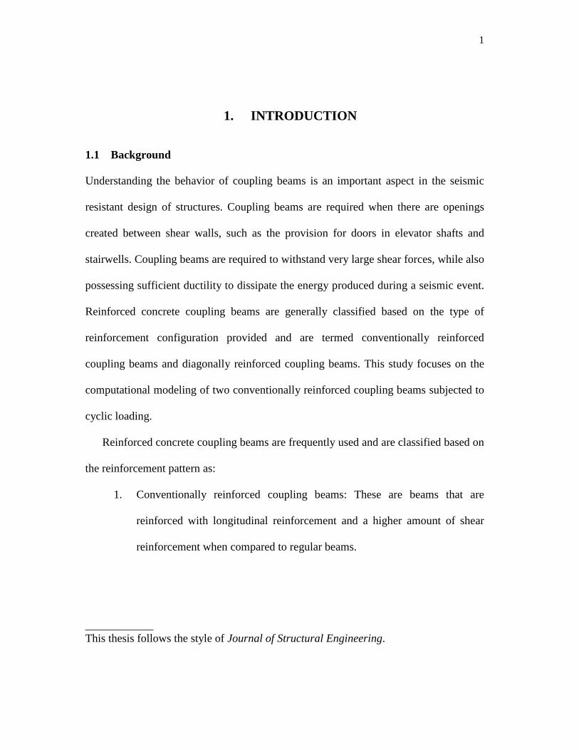
The large shear produced at the face of the connection between the coupling

beam and the shear wall is resisted by provision of large amounts of

transverse reinforcements near this zone. Fig. 1.1 shows a typical layout of

a conventionally reinforced coupling beam.

Fig. 1.1. Typical Layout of Conventionally Reinforced Coupling Beam (Kwan and

Zhao 2002)

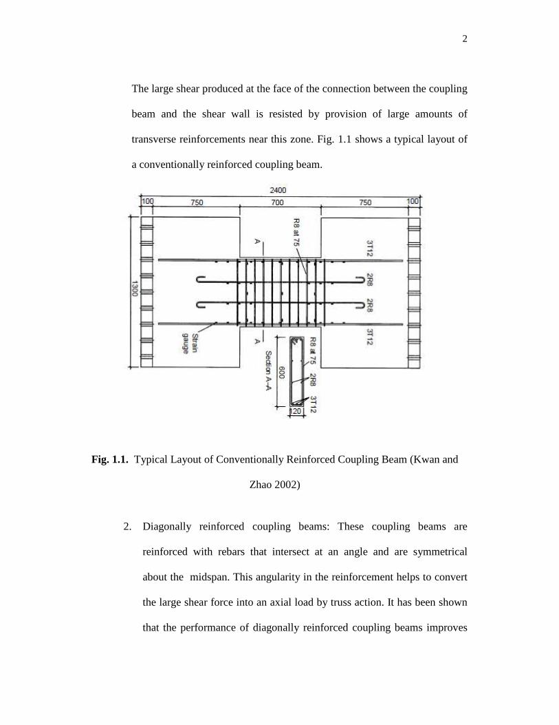
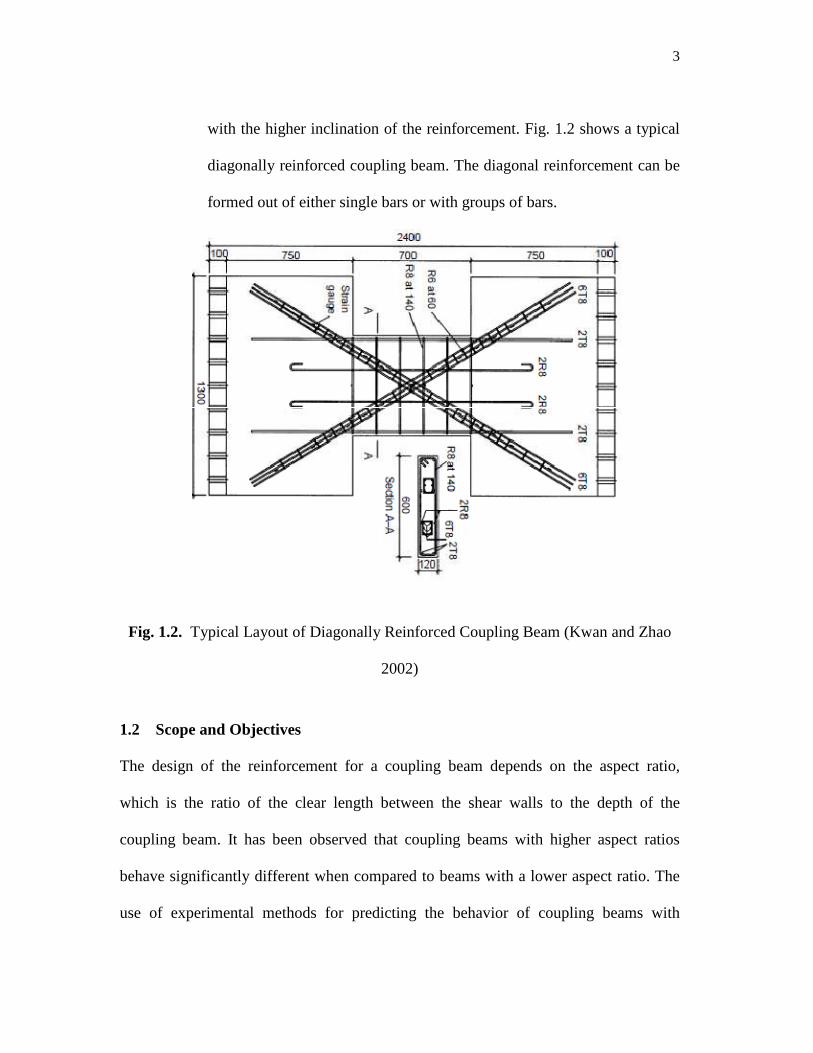
2. Diagonally reinforced coupling beams: These coupling beams are

reinforced with rebars that intersect at an angle and are symmetrical

about the midspan. This angularity in the reinforcement helps to convert

the large shear force into an axial load by truss action. It has been shown

that the performance of diagonally reinforced coupling beams improves

3

with the higher inclination of the reinforcement. Fig. 1.2 shows a typical

diagonally reinforced coupling beam. The diagonal reinforcement can be

formed out of either single bars or with groups of bars.

Fig. 1.2. Typical Layout of Diagonally Reinforced Coupling Beam (Kwan and Zhao

2002)

1.2 Scope and Objectives

The design of the reinforcement for a coupling beam depends on the aspect ratio,

which is the ratio of the clear length between the shear walls to the depth of the

coupling beam. It has been observed that coupling beams with higher aspect ratios

behave significantly different when compared to beams with a lower aspect ratio. The

use of experimental methods for predicting the behavior of coupling beams with

4

varying parameters is both expensive and time consuming. Experimental methods also

provide an additional challenge of duplicating the restraints a coupling beam would

experience during a seismic event. The objective of this work is to produce a

computational model that replicates the behavior of conventionally reinforced coupling

beams subjected to cyclic loading. The computational model should be robust enough

to handle various boundary and load conditions. The computational model will utilize

the concrete damaged plasticity model and will be developed in the finite element

analysis software, ABAQUS (ABAQUS 2008).

1.3 Methodology

The following tasks were performed to accomplish the research objectives:

Task 1: Identification of Experimental Data

The model proposed here is to be tested against experimental results for conventionally

reinforced concrete coupling beams having different aspect ratios and different loading

and test conditions. The two experimental specimens that were chosen for this study

were tested by are Galano and Vignoli (2000) and Bristowe (2000).

Task 2: Establishing Material Properties

The accurate simulation of the experimental results requires that the model replicates

the behavior of the materials involved. The concrete material model was developed

using the modified Popovics equation proposed by Mander et al.(1988). This model

incorporates the effect of confinement on the concrete based on the amount of shear

reinforcement provided. The model has only one equation for both the pre- and post-

5

peak behavior of concrete, making it straightforward to implement in the formulation

of the concrete material behavior.

A key feature of the concrete damaged plasticity model is its ability to predict

the member behavior based on the evolution of damage in the concrete. This requires

an estimate of the variation of the accumulation of damage with respect to the strain in

concrete. The selected damage plasticity constitutive model parameters have been

adopted from Abu Al-Rub and Kim (2010).

Task 3: Parametric Study Using a Calibration Model

An important step before the actual modeling of coupling beams is to obtain a good

estimate of the parameters involved in the damage model and to perform a mesh

refinement study. The dilation angle for the damage model is determined as a key

parameter and is studied in this case. A typical cantilever beam having material

properties similar to the experimental values is modeled using the analysis tool,

RESPONSE 2000 (Bentz 2000). RESPONSE 2000 uses the modified compression

field theory for analyzing the behavior of reinforced concrete members. RESPONSE

2000 is a simple and accurate analytical tool, and was therefore chosen in this study for

determining the behavior of the cantilever model. The force deformation and the

moment curvature response obtained for RESPONSE 2000 are then compared to those

determined using the damage plasticity model generated in ABAQUS. The optimum

values of the dilation angle and the mesh density for the finite element model are

chosen from the results obtained in this study.

6

Task 4: Modeling of the Coupling Beams

The final task is to model the coupling beams in ABAQUS using the material models

and the damage density parameter determined in Task 2 and the results of the

parametric study in Task 3. The coupling beam model was decided to be modeled in

two dimensions as the computational effort required for a three dimensional analysis is

considerably greater. The stress across the section width was assumed to be negligible,

and a plane stress formulation was adopted. Quadratic geometric order elements were

used as the effect of bending is considerable in the problem. Based on the loading

pattern a quasi static analysis is used as the solver option. The results obtained are then

compared to the experimental results. Graphical plots of the force deformation curves,

variation of the stiffness and strength degradation with respect to the cumulative

density, variation of strain along the coupling beam, the evolution and distribution of

the crack pattern and the possible modes of failure are to be obtained from this model.

A comparison of the predictions of the model behavior to the experimental results,

which vary with change in the aspect ratio and loading conditions, is also performed.

1.4 Summary

This research focuses on developing a finite element modeling approach using the

concrete damage plasticity model to replicate the non linear behavior of conventionally

reinforced coupling beams subjected to cyclic loading. An extensive literature review

on the experimental and analytical work for coupling beams is conducted. Based on the

literature review two experimental works are chosen for the process of validating of the

computational model. The parameters to be used for the model are determined using a

7

calibration model. The response of the model using the obtained parameters are

compared to the experimental results.

8

2. LITERATURE REVIEW

2.1 Introduction

The use of shear walls as a construction practice came into effect during the 1950s to

increase the stiffness of a building during an earthquake. These structural members are

required to possess enough resistance and capacity to dissipate the large lateral forces

that can be produced during an earthquake. The design of connecting members for

shear walls was a challenge, as these members not only had to withstand the high

lateral load but also had to possess a higher ductility than that of the walls to prevent

damage to the structure. In a coupled wall structure, the "frame" action of the coupling

beams, that is: the axial forces in the walls resulting from the accumulated shear in the

beams, is typically stiffer than the flexural response of the individual wall piers. As

such, the coupling beams have greater ductility demands than the shear walls.

Coupling beams generally require high amounts of shear reinforcement to be

present at the face of the connection between the coupling beam and the shear walls.

This problem was overcome by an alternate design strategy proposed by Paulay and

Binney (1974). The reinforcement in the proposed "diagonally-reinforced" coupling

beams were placed at an angle to each other. Truss action was developed as a result of

this angular orientation of the reinforcement by which the reinforcement had to resist

only an axial load thereby increasing the coupling beam capacity by a significant

amount. This arrangement of reinforcement allowed for the design to have a lower

amount of transverse reinforcement. The use of other materials like steel plates in the

9

construction of coupling beams is now in practice. These are however beyond the

scope of this report and only reinforced concrete coupling beams are discussed.

2.2 Review of ACI 318 Provisions

The ACI 318-08 building code requirements deal with the design of structural

concrete members (ACI Committee. 318, 2008). A brief study of the primary

requirements related to the design of coupling beams and coupled shear walls has been

made below. Chapter 21 of ACI 318-08 contains requirements for the design and

construction of reinforced concrete structures subjected to earthquake motions, on the

basis of energy dissipation in the nonlinear range of response. Section 21.5 details

requirements related to frame members but these specifications are also recommended

for coupling beams.

2.2.1 Aspect Ratio

Section 21.9.7 of ACI 318-08 addresses coupling beams and the minimum design

requirements. The classification of the coupling beams is made based on the aspect

ratio (i.e., the ratio of the clear distance of the beam ln to the depth of the beam h):

1. Beams with an aspect ratio ln/h > 4 shall satisfy the following requirements

[Section 21.5].

• The factored axial compressive force on the member shall not exceed

Ag f 'c/10 [Section 21.5.1.1].

• The width-to-depth ratio shall not be less than 0.3.

• The width shall not be

o Less than 10 inches.

10

o More than the width of the supporting member plus the distance on each

side of the supporting member should not exceed three-fourths of the

depth of the beam [Section 21.5.1.4].

Sections 21.5.1.3 and 21.5.1.4 are required if the beam does not possess sufficient lateral

stability.

2.2.2 Longitudinal Reinforcement

The amount of reinforcement to be provided in a coupling beam should not be less

then, 200 /b d fw y and the reinforcement ratio shall not exceed 0.025. At least two

bars shall be provided continuously at the top and bottom. The minimum reinforcement

requirements can waived if at every section the area of tensile reinforcement provided

is at least one-third greater than that required by analysis [Section 21.5.2.1].

The positive moment strength at the joint face shall not be less than one-half of

the negative moment strength provided at any face of the joint. Neither the positive or

negative moment strength at any face shall be less than one-fourth of the maximum

moment strength [Section 21.5.2.2].

Lap splices are permitted only if hoop or spiral reinforcement are provided as

they have been found to be more reliable as compared to lap splices of transverse

reinforcement. The maximum spacing of the transverse reinforcement shall not exceed

d/4 or 4 inches [Section 21.5.2.3]. Lap splices shall not be used in the following

locations:

a) Within the joints,

b) Within a distance of twice the member depth from the face of the joint and

11

c) At locations where analysis indicates flexural yielding caused by inelastic

lateral displacement of the frame.

2.2.3 Transverse Reinforcement

Transverse reinforcement are required primarily to confine the concrete and maintain

lateral support for the longitudinal reinforcing bars in regions where yielding is

expected. They are required in the following regions of coupling beams:

a) Over a length equal to twice the member depth measured from the face of

the supporting member towards midspan at both ends of the flexural

member [Section 21.5.3.1],

b) Over a length equal to twice the member depth on both sides of a section

where flexural yielding is likely to occur in connection with inelastic lateral

displacement of the frame.

The first hoop shall be located not more than 2 inches from the face of a supporting

member [Section 21.5.3.2]. The maximum spacing shall not exceed:

a) d/4,

b) eight times the diameter of the smallest longitudinal bars,

c) 24 times the diameter of the hoop bars, and

d) 12 inches.

When hoops are not required, stirrups with seismic hooks at both ends shall be spaced

at a distance not more than d/2 throughout the length of the member [Section 21.5.3.4].

Hoops in flexural members shall be permitted to be made up of two pieces of

reinforcement; a stirrup having seismic hooks at both ends and closed by a crosstie.

12

Consecutive crossties engaging the same longitudinal bar shall have their 90 degrees

hooks at opposite sides of the flexural member. If the longitudinal reinforcing bars

secured by the crossties are confined by the slabs on only one side of the flexural

coupling beam, the 90 degree hooks of the crossties shall be place on that side [Section

21.5.3.6].

2.2.4 Shear Strength Requirements

The design shear force, Ve, corresponding to the equivalent lateral force representing

the earthquake, shall be determined shall from consideration of the statical forces on

the portion of the member between faces of the joints. It shall be assumed that

moments of opposite sign corresponding to the probable flexural moment strength, Mpr

act at the joint faces and that the member is loaded with factored tributary gravity load

along its span. It is assumed the frames dissipate the earthquake energy in a nonlinear

range of response. Unless the frame is designed for 3-4 times the design force it is

assumed to yield in the event of major earthquake. The required shear strength of a

coupling beam is related to the flexural strength of the designed members rather than

the factored shear force.

2.2.5 Transverse Reinforcement for Shear Strength

From experimental studies it has been shown that more shear reinforcement is required

to ensure that members fail in flexure first when subjected to cyclic loading. The

necessity of an increase of shear reinforcement is higher when there is absence of axial

load is reflected in the requirements as per Section 21.5.4.2 according to which

13

transverse reinforcement shall be portioned to resist shear assuming Vc = 0 when both

of the following conditions occur:

a) The earthquake induced shear force calculated represents one half or more

of the maximum required shear strength with those lengths;

b) The factored axial compressive force inclining earthquake force is less then

Agf 'c /20.

Coupling beams with aspect ratio ln/h < 4 are permitted to be reinforced with two

intersecting groups of diagonally placed bars symmetrical about midspan [Section

21.9.7.2].

Coupling beams with an aspect ratio ln/h<2 with a factored shear force Vu

exceeding '4 c cpf A (in-lb units) shall be reinforced with two intersecting bars of

diagonally placed bars symmetrical about the midspan, unless it can be shown that the

loss of stiffness and the strength will not impair the vertical load carrying capacity of

the structure or egress from the structure, or the integrity of nonstructural components

[Section 21.9.7.3].

2.3 Experimental Research

2.3.1 Coupling Beam Failure Modes

This section presents a review of experimental research on reinforced concrete

coupling beams. Various types of failures observed in coupling beam tests are

discussed in this section including the following:

14

• Shear compression (SC): This failure is usually seen in conventionally

reinforced coupling beams. The beams fail at the junction of coupling beams

with the shear walls. The concrete is crushed at these points when the stress is

above the concrete compressive strength.

• Shear Sliding (SS): This failure is usually observed in conventionally

reinforced coupling beams. A large amount of shear stress is produced between

the connection between the shear wall and the coupling beams. This is found to

happen when the shear strength of the reinforcement is lower than the shear

stress at the joint.

• Flexural Failure (FF): This is a general case of failure for beam with

insufficient flexural strength. These failures are seen particularly in the case of

conventionally reinforced coupling beams.

• Shear Tension (ST): This failure is seen usually in conventionally reinforced

coupling beams. The beams fail at the junction of coupling beams with the

shear walls. The concrete cracks when the tensile demands on concrete exceed

the cracking stress capacity.

• Buckling of Diagonal Reinforcement (BDR): This failure is seen in diagonally

reinforced coupling beams. The diagonal reinforcement are provided to convert

the high amount of shear reinforcement into axial compression/tension. When

the compression demands on the reinforcement exceed the buckling load, the

beams fail.

15

• Local Diagonal Reinforcement Failure (LD): This failure occurs in beams with

diagonal reinforcement only at joints between shear walls and coupling beam.

The diagonal reinforcement fails either in tension or compression causing a

failure in the coupling beam.

• Diagonal Tension (DT): If the axial tension in the diagonal reinforcement is

higher than the axial strength of the reinforcement, the coupling beams fail.

2.3.2 Summary of Experimental Research Work

Tables 2.1 and 2.2 summarize the experimental research work done in the field of

coupling beams. Key parameters are provided for each specimen followed by a

description of key points in each of the research studies.

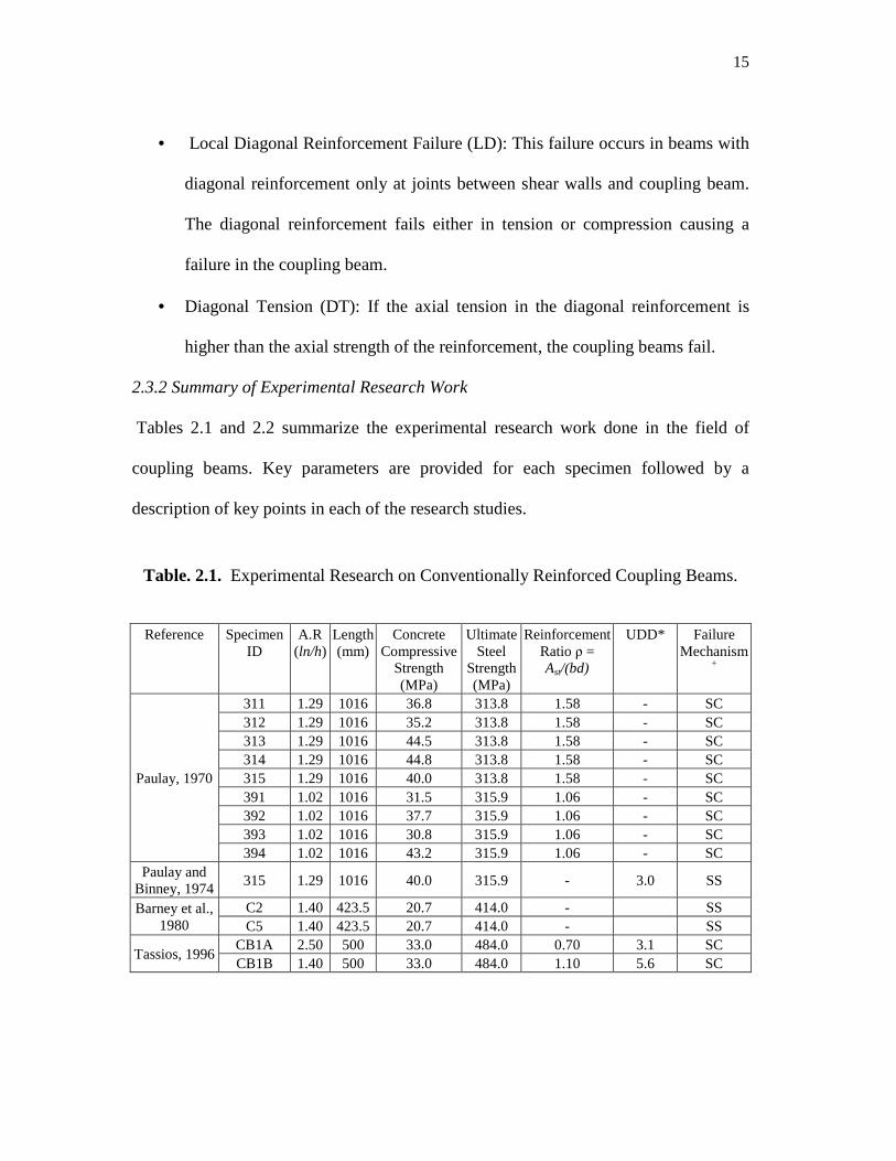
Table. 2.1. Experimental Research on Conventionally Reinforced Coupling Beams.

Reference Specimen ID

A.R (ln/h)

Length (mm)

Concrete Compressive

Strength (MPa)

Ultimate Steel

Strength (MPa)

Reinforcement Ratio ρ = Ast/(bd)

UDD* Failure Mechanism

+

Paulay, 1970

311 1.29 1016 36.8 313.8 1.58 - SC 312 1.29 1016 35.2 313.8 1.58 - SC 313 1.29 1016 44.5 313.8 1.58 - SC 314 1.29 1016 44.8 313.8 1.58 - SC 315 1.29 1016 40.0 313.8 1.58 - SC 391 1.02 1016 31.5 315.9 1.06 - SC 392 1.02 1016 37.7 315.9 1.06 - SC 393 1.02 1016 30.8 315.9 1.06 - SC 394 1.02 1016 43.2 315.9 1.06 - SC

Paulay and Binney, 1974

315 1.29 1016 40.0 315.9 - 3.0 SS

Barney et al., 1980

C2 1.40 423.5 20.7 414.0 -

SS C5 1.40 423.5 20.7 414.0 -

SS

Tassios, 1996 CB1A 2.50 500 33.0 484.0 0.70 3.1 SC CB1B 1.40 500 33.0 484.0 1.10 5.6 SC

16

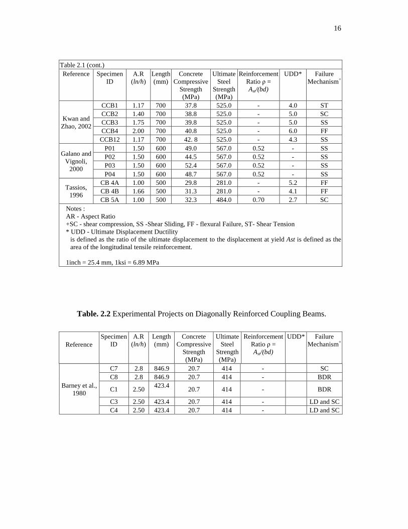
Table 2.1 (cont.) Reference Specimen

ID A.R

(ln/h) Length (mm)


Strength (MPa)

Ultimate Steel

Strength (MPa)


UDD* Failure Mechanism+

Kwan and Zhao, 2002

CCB1 1.17 700 37.8 525.0 - 4.0 ST CCB2 1.40 700 38.8 525.0 - 5.0 SC CCB3 1.75 700 39.8 525.0 - 5.0 SS CCB4 2.00 700 40.8 525.0 - 6.0 FF CCB12 1.17 700 42. 8 525.0 - 4.3 SS

Galano and Vignoli,

2000

P01 1.50 600 49.0 567.0 0.52 - SS P02 1.50 600 44.5 567.0 0.52 - SS P03 1.50 600 52.4 567.0 0.52 - SS P04 1.50 600 48.7 567.0 0.52 - SS

Tassios, 1996

CB 4A 1.00 500 29.8 281.0 - 5.2 FF CB 4B 1.66 500 31.3 281.0 - 4.1 FF CB 5A 1.00 500 32.3 484.0 0.70 2.7 SC

Notes : AR - Aspect Ratio +SC - shear compression, SS -Shear Sliding, FF - flexural Failure, ST- Shear Tension * UDD - Ultimate Displacement Ductility

is defined as the ratio of the ultimate displacement to the displacement at yield Ast is defined as the area of the longitudinal tensile reinforcement.

1inch = 25.4 mm, 1ksi = 6.89 MPa

Table. 2.2 Experimental Projects on Diagonally Reinforced Coupling Beams.

Reference Specimen

ID A.R

(ln/h) Length (mm)


Strength (MPa)

Ultimate Steel

Strength (MPa)



Barney et al., 1980

C7 2.8 846.9 20.7 414 - SC C8 2.8 846.9 20.7 414 - BDR

C1 2.50 423.4

20.7 414 - BDR

C3 2.50 423.4 20.7 414 - LD and SC C4 2.50 423.4 20.7 414 - LD and SC

17

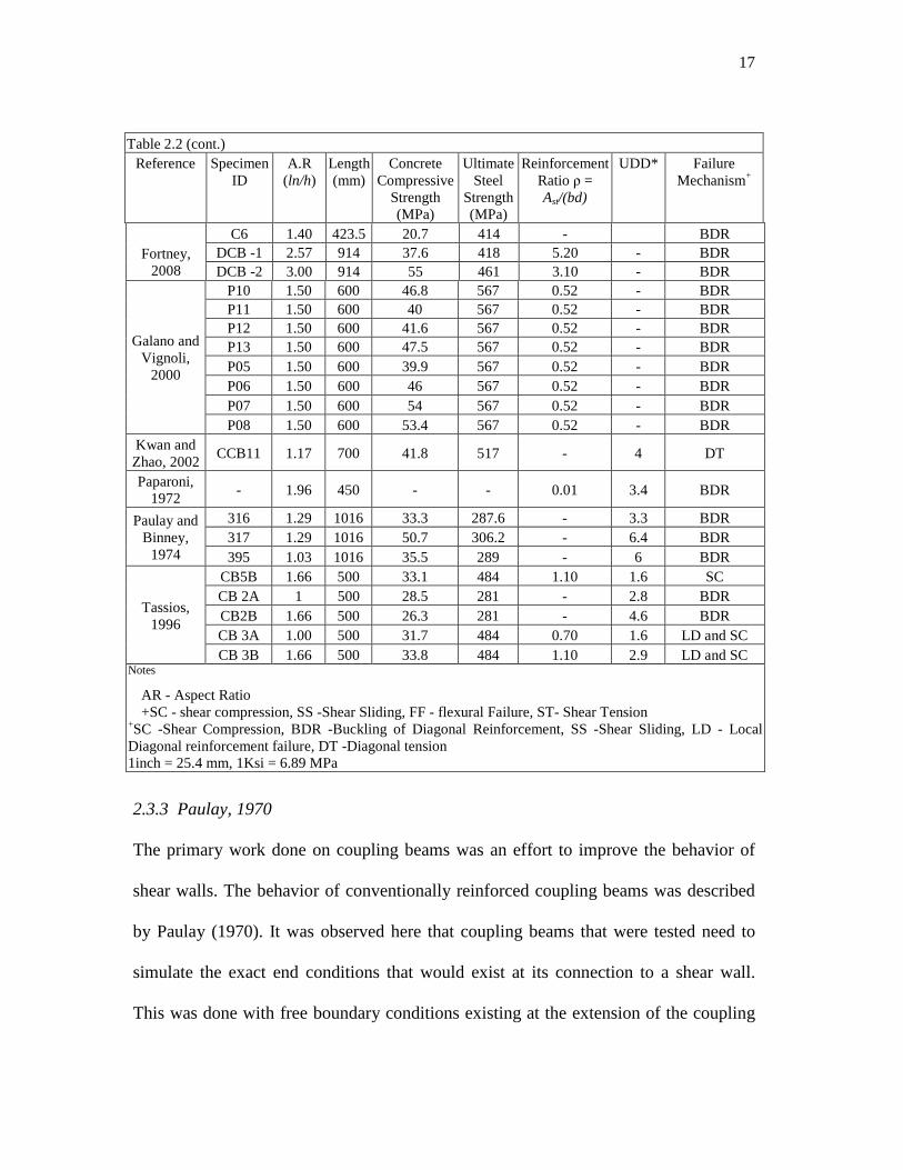
Table 2.2 (cont.) Reference Specimen

ID A.R

(ln/h) Length (mm)


Strength (MPa)

Ultimate Steel

Strength (MPa)



C6 1.40 423.5 20.7 414 - BDR

Fortney, 2008

DCB -1 2.57 914 37.6 418 5.20 - BDR DCB -2 3.00 914 55 461 3.10 - BDR

Galano and Vignoli,

2000

P10 1.50 600 46.8 567 0.52 - BDR P11 1.50 600 40 567 0.52 - BDR P12 1.50 600 41.6 567 0.52 - BDR P13 1.50 600 47.5 567 0.52 - BDR P05 1.50 600 39.9 567 0.52 - BDR P06 1.50 600 46 567 0.52 - BDR P07 1.50 600 54 567 0.52 - BDR P08 1.50 600 53.4 567 0.52 - BDR

Kwan and Zhao, 2002

CCB11 1.17 700 41.8 517 - 4 DT

Paparoni, 1972

- 1.96 450 - - 0.01 3.4 BDR

Paulay and Binney,

1974

316 1.29 1016 33.3 287.6 - 3.3 BDR 317 1.29 1016 50.7 306.2 - 6.4 BDR 395 1.03 1016 35.5 289 - 6 BDR

Tassios, 1996

CB5B 1.66 500 33.1 484 1.10 1.6 SC CB 2A 1 500 28.5 281 - 2.8 BDR CB2B 1.66 500 26.3 281 - 4.6 BDR CB 3A 1.00 500 31.7 484 0.70 1.6 LD and SC CB 3B 1.66 500 33.8 484 1.10 2.9 LD and SC

Notes

AR - Aspect Ratio +SC - shear compression, SS -Shear Sliding, FF - flexural Failure, ST- Shear Tension

+SC -Shear Compression, BDR -Buckling of Diagonal Reinforcement, SS -Shear Sliding, LD - Local Diagonal reinforcement failure, DT -Diagonal tension 1inch = 25.4 mm, 1Ksi = 6.89 MPa

2.3.3 Paulay, 1970

The primary work done on coupling beams was an effort to improve the behavior of

shear walls. The behavior of conventionally reinforced coupling beams was described

by Paulay (1970). It was observed here that coupling beams that were tested need to

simulate the exact end conditions that would exist at its connection to a shear wall.

This was done with free boundary conditions existing at the extension of the coupling

18

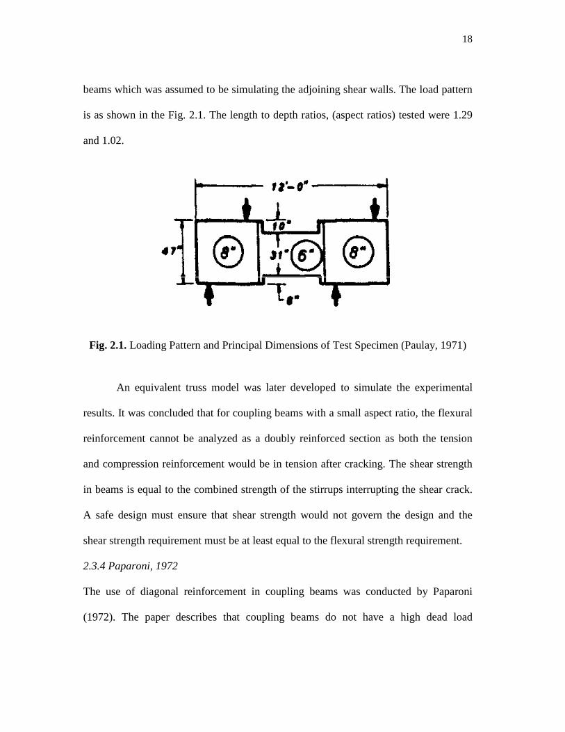
beams which was assumed to be simulating the adjoining shear walls. The load pattern

is as shown in the Fig. 2.1. The length to depth ratios, (aspect ratios) tested were 1.29

and 1.02.

Fig. 2.1. Loading Pattern and Principal Dimensions of Test Specimen (Paulay, 1971)

An equivalent truss model was later developed to simulate the experimental

results. It was concluded that for coupling beams with a small aspect ratio, the flexural

reinforcement cannot be analyzed as a doubly reinforced section as both the tension

and compression reinforcement would be in tension after cracking. The shear strength

in beams is equal to the combined strength of the stirrups interrupting the shear crack.

A safe design must ensure that shear strength would not govern the design and the

shear strength requirement must be at least equal to the flexural strength requirement.

2.3.4 Paparoni, 1972

The use of diagonal reinforcement in coupling beams was conducted by Paparoni

(1972). The paper describes that coupling beams do not have a high dead load

19

requirement but they do need to possess enough stiffness and shear strength to resist

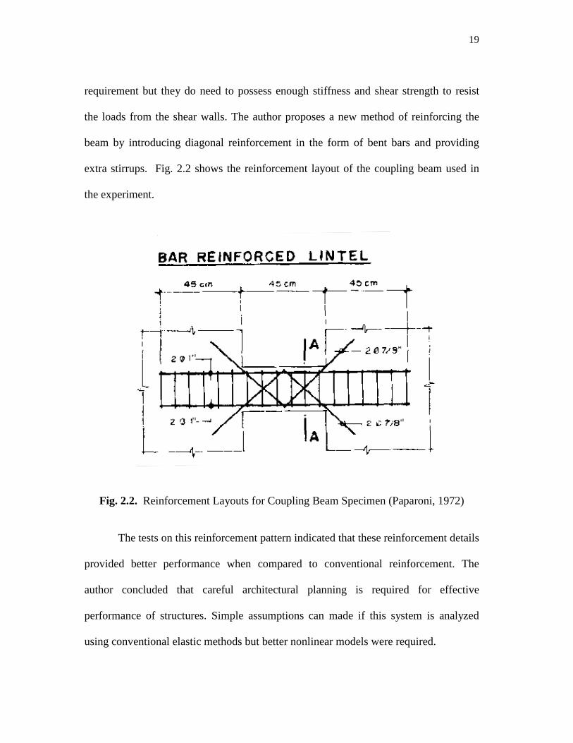
the loads from the shear walls. The author proposes a new method of reinforcing the

beam by introducing diagonal reinforcement in the form of bent bars and providing

extra stirrups. Fig. 2.2 shows the reinforcement layout of the coupling beam used in

the experiment.

Fig. 2.2. Reinforcement Layouts for Coupling Beam Specimen (Paparoni, 1972)

The tests on this reinforcement pattern indicated that these reinforcement details

provided better performance when compared to conventional reinforcement. The

author concluded that careful architectural planning is required for effective

performance of structures. Simple assumptions can made if this system is analyzed

using conventional elastic methods but better nonlinear models were required.

20

2.3.5 Paulay and Binney, 1974

Paulay and Binney (1974) conducted the initial work to make use of the truss action

provided by inclined reinforcement. The authors described that the diagonal

reinforcement would convert the large amounts of shear produced into axial forces

acting along the length of the members. Reinforcing steel, which possess a higher axial

tensile and compressive capability, enhances the strength of the coupling beam to a

great extent. This formed a major breakthrough in the design of coupling beams. The

diagonal reinforcement also increased the ductility of the beam when compared to a

conventional reinforced coupling beam. Although research on the subject of diagonal

reinforced coupling beams was started in the early 1970s, the provision for this

reinforcements appeared in codes of practice much later.

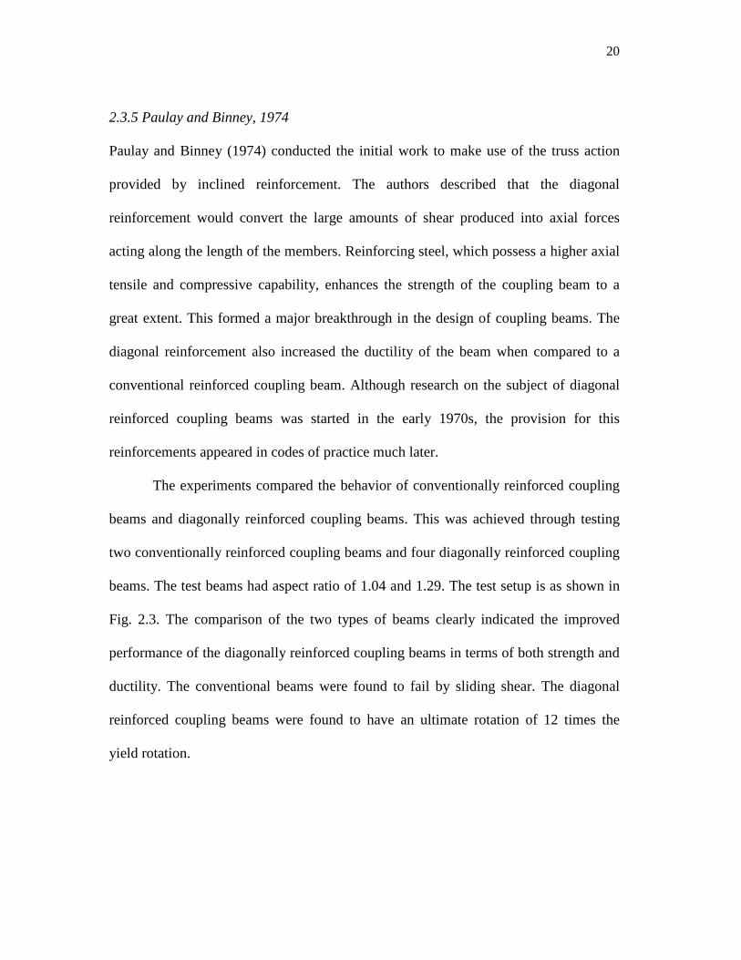
The experiments compared the behavior of conventionally reinforced coupling

beams and diagonally reinforced coupling beams. This was achieved through testing

two conventionally reinforced coupling beams and four diagonally reinforced coupling

beams. The test beams had aspect ratio of 1.04 and 1.29. The test setup is as shown in

Fig. 2.3. The comparison of the two types of beams clearly indicated the improved

performance of the diagonally reinforced coupling beams in terms of both strength and

ductility. The conventional beams were found to fail by sliding shear. The diagonal

reinforced coupling beams were found to have an ultimate rotation of 12 times the

yield rotation.

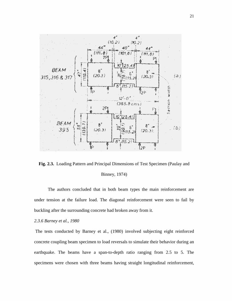
Fig. 2.3. Loading Pattern and Principal Dimensions of Test Specimen (Paulay

The authors conclude

under tension at the failure load. The diagonal reinforcement were seen to fail by

buckling after the surrounding concrete had broken away from it.

2.3.6 Barney et al., 1980

The tests conducted by Barney

concrete coupling beam specimen

earthquake. The beams have a span

specimens were chosen with three beams having straight longitudinal reinforcement,

ng Pattern and Principal Dimensions of Test Specimen (Paulay

Binney, 1974)

The authors concluded that in both beam types the main reinforcement are

failure load. The diagonal reinforcement were seen to fail by

urrounding concrete had broken away from it.

Barney et al., (1980) involved subjecting eight reinforced

specimen to load reversals to simulate their behavior during an

have a span-to-depth ratio ranging from 2.5 to 5. The


21

ng Pattern and Principal Dimensions of Test Specimen (Paulay and

the main reinforcement are

failure load. The diagonal reinforcement were seen to fail by

involved subjecting eight reinforced

to simulate their behavior during an

depth ratio ranging from 2.5 to 5. The


22

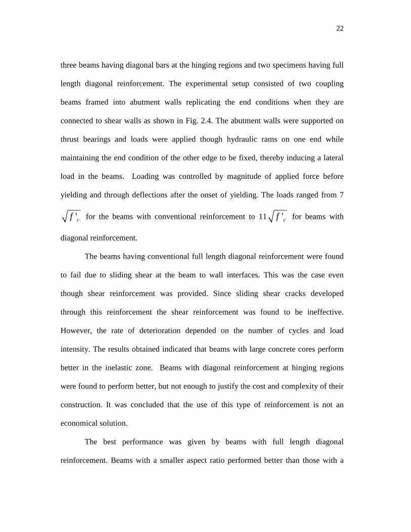
three beams having diagonal bars at the hinging regions and two specimens having full

length diagonal reinforcement. The experimental setup consisted of two coupling

beams framed into abutment walls replicating the end conditions when they are

connected to shear walls as shown in Fig. 2.4. The abutment walls were supported on

thrust bearings and loads were applied though hydraulic rams on one end while

maintaining the end condition of the other edge to be fixed, thereby inducing a lateral

load in the beams. Loading was controlled by magnitude of applied force before

yielding and through deflections after the onset of yielding. The loads ranged from 7

cf ' for the beams with conventional reinforcement to 11 cf ' for beams with

diagonal reinforcement.

The beams having conventional full length diagonal reinforcement were found

to fail due to sliding shear at the beam to wall interfaces. This was the case even

though shear reinforcement was provided. Since sliding shear cracks developed

through this reinforcement the shear reinforcement was found to be ineffective.

However, the rate of deterioration depended on the number of cycles and load

intensity. The results obtained indicated that beams with large concrete cores perform

better in the inelastic zone. Beams with diagonal reinforcement at hinging regions

were found to perform better, but not enough to justify the cost and complexity of their

construction. It was concluded that the use of this type of reinforcement is not an

economical solution.

The best performance was given by beams with full length diagonal

reinforcement. Beams with a smaller aspect ratio performed better than those with a

23

larger aspect ratio. The test also revealed that gravity loads play an important role in

the performance of diagonally reinforced concrete members and an ideal aspect ratio

ranges from 1.4 to 2.8. The reinforcement also need to be well anchored for superior

performance. It is also suggested that actual capacity of the beams be used as a way to

test the beam strengths rather than the yield levels of the materials.

Fig. 2.4. Boundary Condition of the Specimen (Barney et al., 1980)

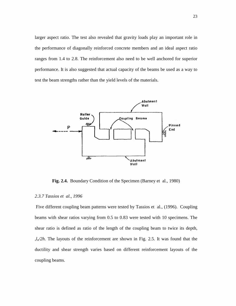
2.3.7 Tassios et al., 1996

Five different coupling beam patterns were tested by Tassios et al., (1996). Coupling

beams with shear ratios varying from 0.5 to 0.83 were tested with 10 specimens. The

shear ratio is defined as ratio of the length of the coupling beam to twice its depth,

,ln/2h. The layouts of the reinforcement are shown in Fig. 2.5. It was found that the

ductility and shear strength varies based on different reinforcement layouts of the

coupling beams.

24

Fig. 2.5. Reinforcement Layouts for Coupling Beam Specimens (Tassios et al., 1996)

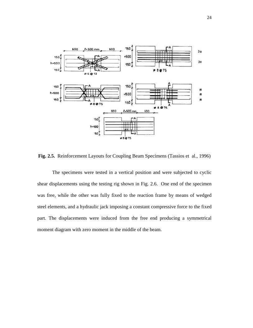
The specimens were tested in a vertical position and were subjected to cyclic

shear displacements using the testing rig shown in Fig. 2.6. One end of the specimen

was free, while the other was fully fixed to the reaction frame by means of wedged

steel elements, and a hydraulic jack imposing a constant compressive force to the fixed

part. The displacements were induced from the free end producing a symmetrical

moment diagram with zero moment in the middle of the beam.

25

Fig. 2.6. Boundary Condition and Testing Mechanism for Coupling Beam Specimen

(Tassios et al.,1996)

It was found that the specimen with diagonally reinforcement showed better

performance among the tested beams. The introduction of bent-up bars led to an

increased ultimate capacity and overall behavior compared to conventionally

reinforced beams. The specimens with short dowels did not exhibit any sliding at their

ends. However, they were found to be the most brittle among all the specimens tested.

The specimens with long dowels behaved slightly better than the specimens with short

dowels. The authors conclude by saying that members with a higher shear ratio had a

higher ductility compared to the ones with a lower shear ratio. A shear ratio of 0.75 is

optimum for a diagonally reinforced beam.

2.3.8 Galano and Vignoli, 2000

Galano and Vignoli (2000) tested 15 coupling beams having an aspect ratio of 1.5 and

with varying reinforcement patterns and loading histories. The loading pattern was

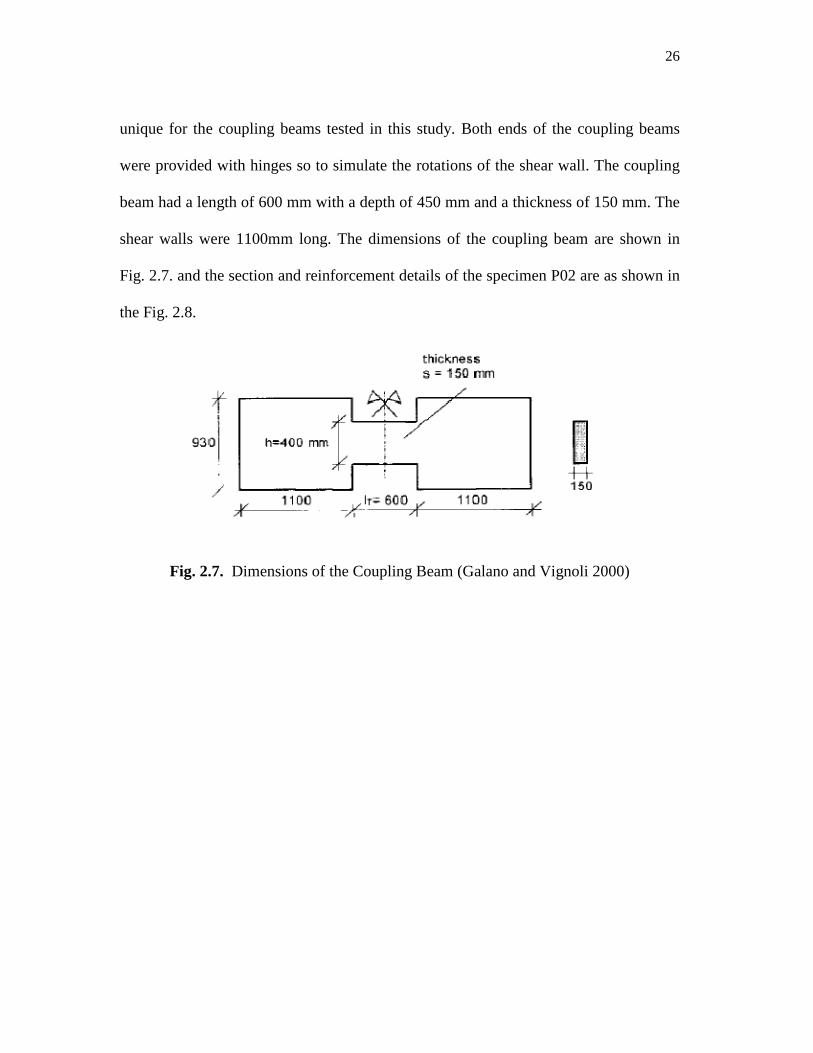
26

unique for the coupling beams tested in this study. Both ends of the coupling beams

were provided with hinges so to simulate the rotations of the shear wall. The coupling

beam had a length of 600 mm with a depth of 450 mm and a thickness of 150 mm. The

shear walls were 1100mm long. The dimensions of the coupling beam are shown in

Fig. 2.7. and the section and reinforcement details of the specimen P02 are as shown in

the Fig. 2.8.

Fig. 2.7. Dimensions of the Coupling Beam (Galano and Vignoli 2000)

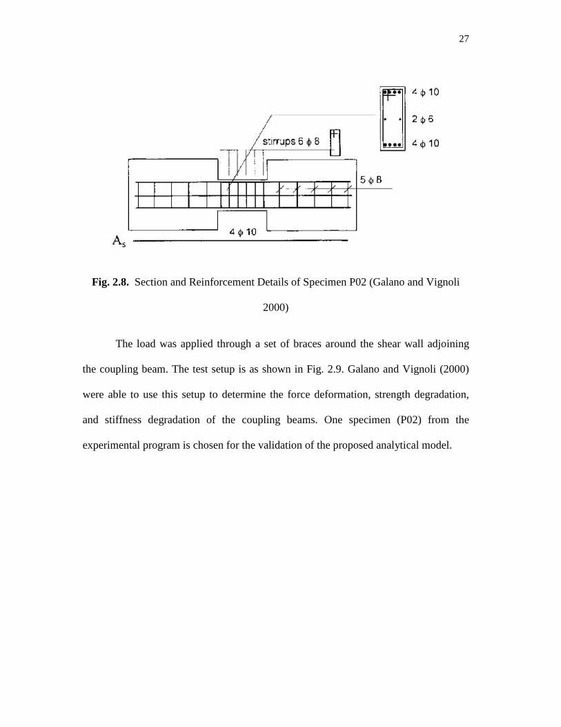
27

Fig. 2.8. Section and Reinforcement Details of Specimen P02 (Galano and Vignoli

2000)

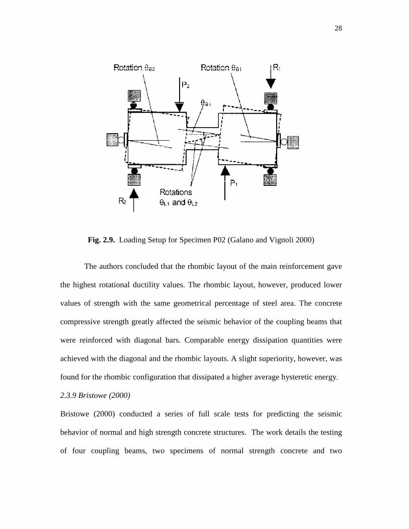
The load was applied through a set of braces around the shear wall adjoining

the coupling beam. The test setup is as shown in Fig. 2.9. Galano and Vignoli (2000)

were able to use this setup to determine the force deformation, strength degradation,

and stiffness degradation of the coupling beams. One specimen (P02) from the

experimental program is chosen for the validation of the proposed analytical model.

28

Fig. 2.9. Loading Setup for Specimen P02 (Galano and Vignoli 2000)

The authors concluded that the rhombic layout of the main reinforcement gave

the highest rotational ductility values. The rhombic layout, however, produced lower

values of strength with the same geometrical percentage of steel area. The concrete

compressive strength greatly affected the seismic behavior of the coupling beams that

were reinforced with diagonal bars. Comparable energy dissipation quantities were

achieved with the diagonal and the rhombic layouts. A slight superiority, however, was

found for the rhombic configuration that dissipated a higher average hysteretic energy.

2.3.9 Bristowe (2000)

Bristowe (2000) conducted a series of full scale tests for predicting the seismic

behavior of normal and high strength concrete structures. The work details the testing

of four coupling beams, two specimens of normal strength concrete and two

29

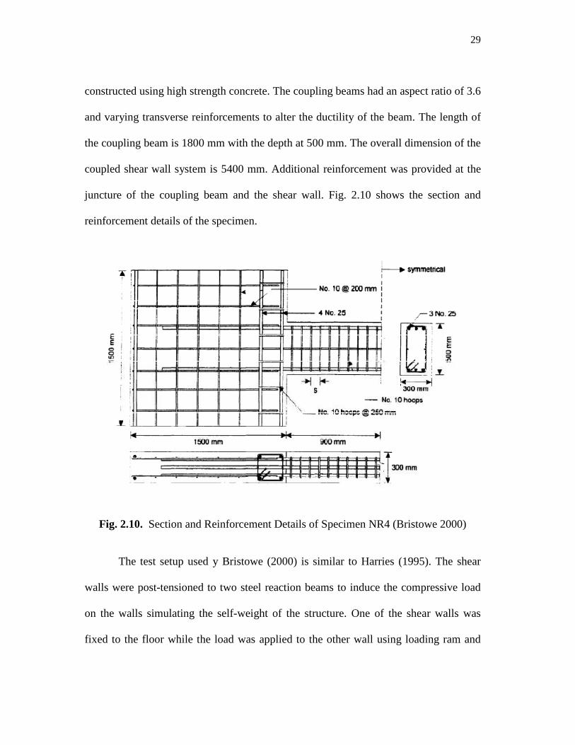
constructed using high strength concrete. The coupling beams had an aspect ratio of 3.6

and varying transverse reinforcements to alter the ductility of the beam. The length of

the coupling beam is 1800 mm with the depth at 500 mm. The overall dimension of the

coupled shear wall system is 5400 mm. Additional reinforcement was provided at the

juncture of the coupling beam and the shear wall. Fig. 2.10 shows the section and

reinforcement details of the specimen.

Fig. 2.10. Section and Reinforcement Details of Specimen NR4 (Bristowe 2000)

The test setup used y Bristowe (2000) is similar to Harries (1995). The shear

walls were post-tensioned to two steel reaction beams to induce the compressive load

on the walls simulating the self-weight of the structure. One of the shear walls was

fixed to the floor while the load was applied to the other wall using loading ram and

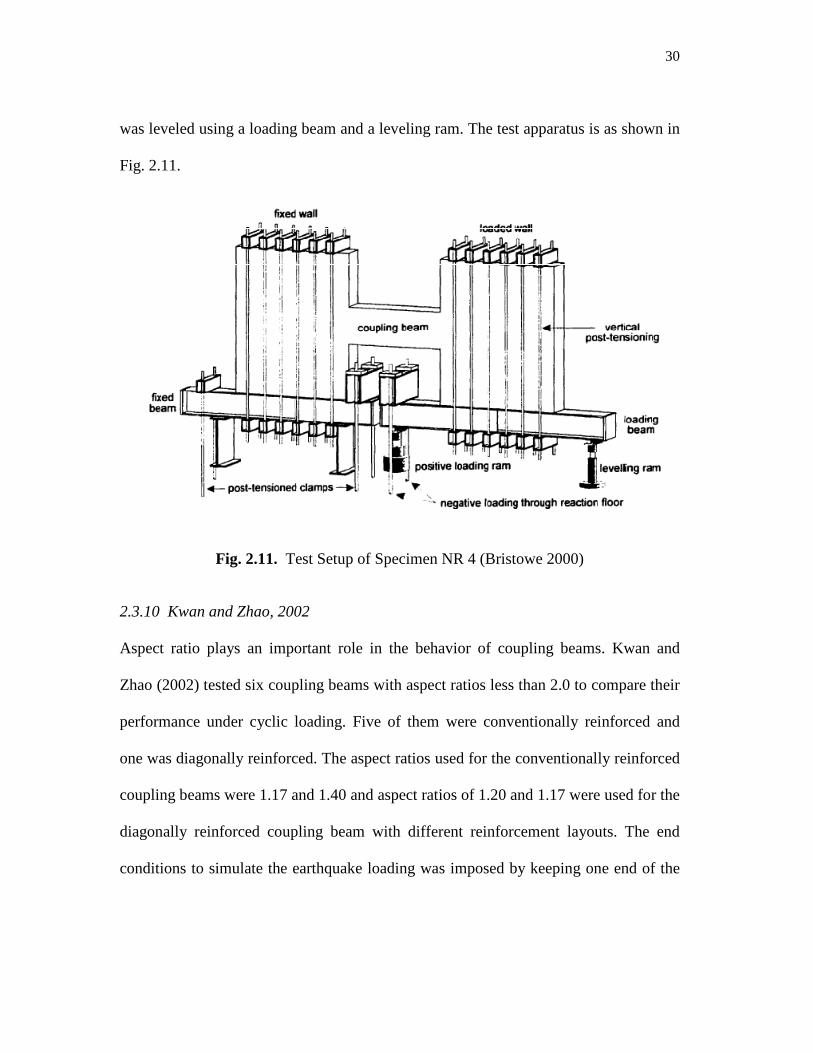
30

was leveled using a loading beam and a leveling ram. The test apparatus is as shown in

Fig. 2.11.

Fig. 2.11. Test Setup of Specimen NR 4 (Bristowe 2000)

2.3.10 Kwan and Zhao, 2002

Aspect ratio plays an important role in the behavior of coupling beams. Kwan and

Zhao (2002) tested six coupling beams with aspect ratios less than 2.0 to compare their

performance under cyclic loading. Five of them were conventionally reinforced and

one was diagonally reinforced. The aspect ratios used for the conventionally reinforced

coupling beams were 1.17 and 1.40 and aspect ratios of 1.20 and 1.17 were used for the

diagonally reinforced coupling beam with different reinforcement layouts. The end

conditions to simulate the earthquake loading was imposed by keeping one end of the

31

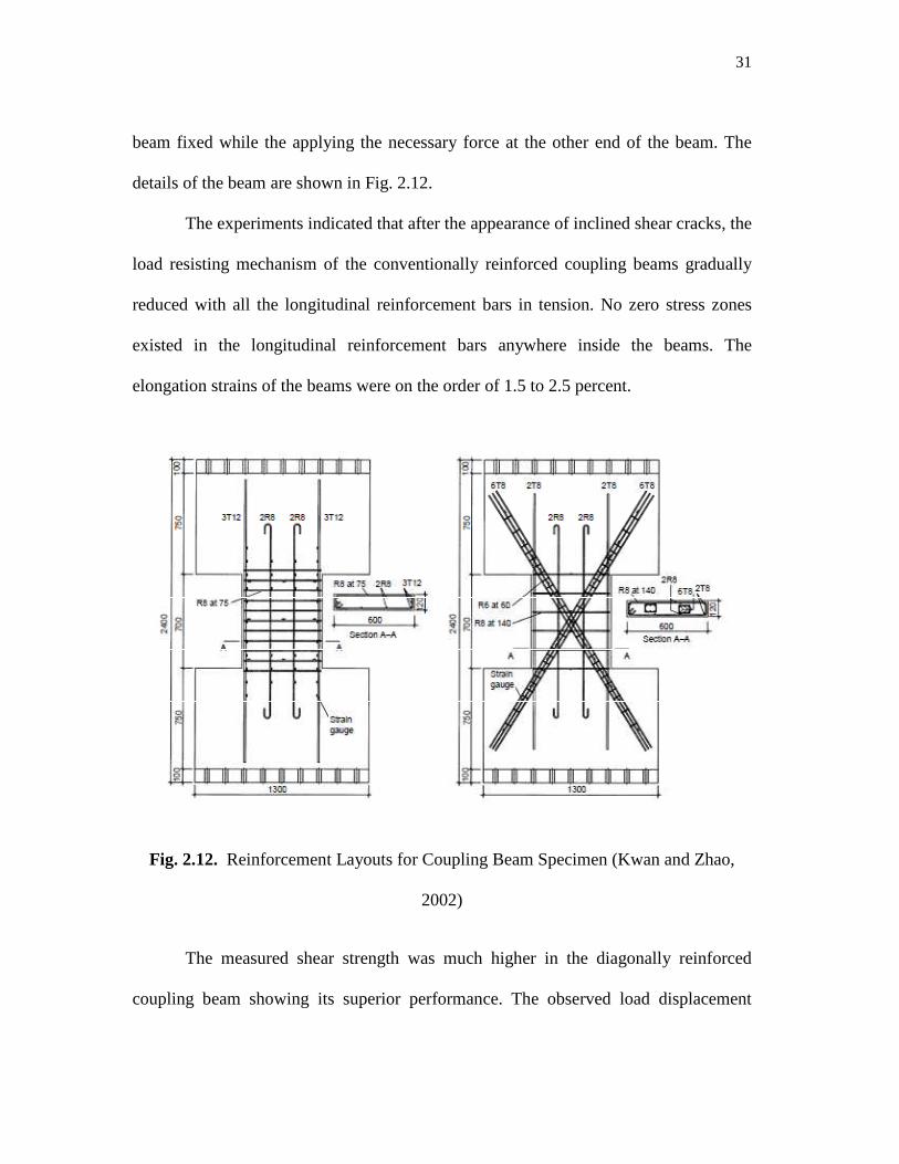
beam fixed while the applying the necessary force at the other end of the beam. The

details of the beam are shown in Fig. 2.12.

The experiments indicated that after the appearance of inclined shear cracks, the

load resisting mechanism of the conventionally reinforced coupling beams gradually

reduced with all the longitudinal reinforcement bars in tension. No zero stress zones

existed in the longitudinal reinforcement bars anywhere inside the beams. The

elongation strains of the beams were on the order of 1.5 to 2.5 percent.

Fig. 2.12. Reinforcement Layouts for Coupling Beam Specimen (Kwan and Zhao,

2002)

The measured shear strength was much higher in the diagonally reinforced

coupling beam showing its superior performance. The observed load displacement

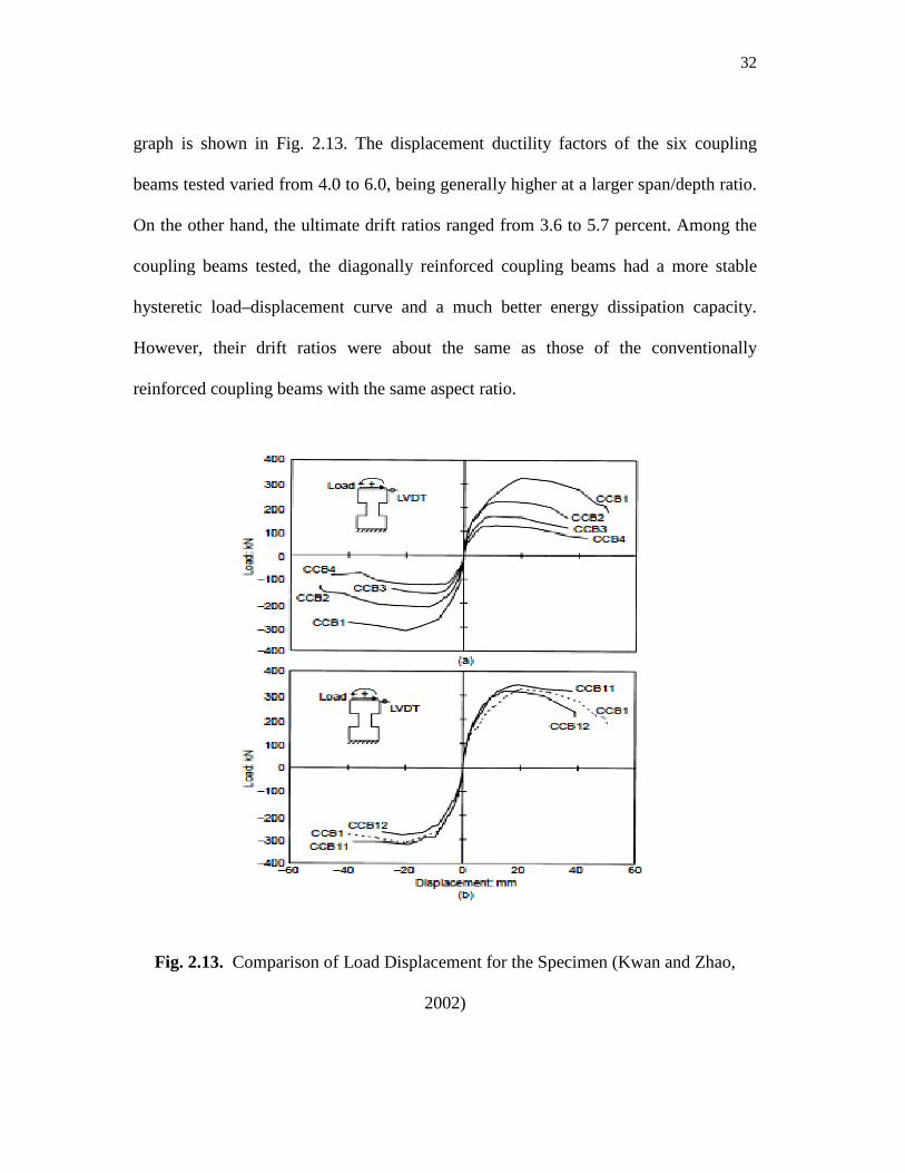
graph is shown in Fig. 2.13

beams tested varied from 4.0 to 6

On the other hand, the ultimate drift ratios ranged from 3

coupling beams tested, the diagonally reinforced coupling beams had a more stable

hysteretic load–displacement curve and a much better energy dissipation capacity.

However, their drift ratios were about the same as those of the conventionally

reinforced coupling beams with the same aspect ratio.

Fig. 2.13. Comparison of Load Displacement for the Specimen (Kwan and Zhao,

3. The displacement ductility factors of the six coupling

0 to 6.0, being generally higher at a larger span/depth ratio.

On the other hand, the ultimate drift ratios ranged from 3.6 to 5.7 percent. Among the


displacement curve and a much better energy dissipation capacity.

drift ratios were about the same as those of the conventionally

reinforced coupling beams with the same aspect ratio.

Comparison of Load Displacement for the Specimen (Kwan and Zhao,

2002)

32

The displacement ductility factors of the six coupling

0, being generally higher at a larger span/depth ratio.

. Among the


displacement curve and a much better energy dissipation capacity.

drift ratios were about the same as those of the conventionally

Comparison of Load Displacement for the Specimen (Kwan and Zhao,

33

Baczkowski and Kaung (2008) proposed a new technique for testing of

coupling beams to overcome some of the shortfalls of the earlier experiments. The

authors discuss in detail earlier experiments and their deficiencies and validate the new

testing methodology proposed.

The earliest method of testing coupling beams was developed by Paulay and

Biney (1974) where the loads were applied through hydraulic actuators with welded

loading trusses. The walls connected by the coupling beams are rotated as to simulate

the effect produced by tall building subjected to a lateral load. However the simulation

of the boundary condition to ensure equal rotation of the walls is inefficient. This

approach was modified in the test method developed by Barney et al. (1980). Two

coupling beams were built in between abutment walls. One of the abutment walls was

connected to a roller guide while keeping the other end pinned. The load was applied

through the roller guides. The walls remain parallel during the test so to allow equal

rotation of the coupling beams simulating the ideal boundary condition. However the

apparatus uses a considerable amount of the space in the laboratory and the size

requires the use of powerful actuators to apply the load. Harris et al. (1993) proposed

another method of testing coupling beams wherein the beams were placed in between

shear walls. Shear force was then applied to one of the walls in the direction

perpendicular to the test beam keeping the other beam fixed. This method mainly finds

its application in testing shallow and slender beams.

The test rig proposed is built on a mechanism that loads the beam by deflecting

the end walls to rotate equally. The beam is built in between two abutment walls and

34

the load is applied through a hydraulic actuator on the top of the shear walls while

keeping the bottom support of the wall fixed. The actuator is fixed to the strong

reaction wall and carries its own weight as a cantilever. The walls are connected to the

actuator and the steel base by using hinge beams to adjust to a convenient position. The

horizontal load is transferred from actuators to the top of hinge beam and is resisted by

the bottom hinges. This creates a horizontal couple causing an overturning moment.

The moment in the hinge is transferred to the walls by a vertical couple force

subsequently acting as shear in the beam. This replicates the shear force experienced by

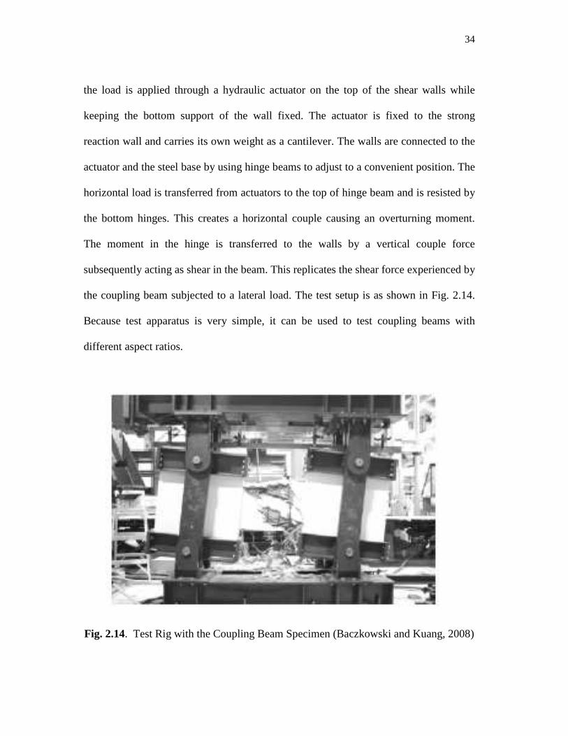
the coupling beam subjected to a lateral load. The test setup is as shown in Fig. 2.14.

Because test apparatus is very simple, it can be used to test coupling beams with

different aspect ratios.

Fig. 2.14. Test Rig with the Coupling Beam Specimen (Baczkowski and Kuang, 2008)

35

The apparatus was now tested with three specimens of varying aspect ratio. The

beams were chosen with aspect ratios of 1, 1.5 and 2. The loading was applied by

controlling the load in the first stage and using displacement-control in the second

stage. The hydraulic actuators were used to produce the required amount of reversed

cyclic loading. The new test rig was found to have the following advantages:

• The boundary condition is well incorporated in the loading rig mechanism.

• There is conveyance of testing coupling beams of various aspect ratios without

modifying the apparatus by a large degree.

• The cost of construction is cheaper compared to the other methods of testing.

2.3.11 Fortney et al, 2008

The transverse reinforcement in coupling beams play an important role in the strength

of conventional reinforced concrete coupling beams. The experiment by Fortnet et, al.

(2008) compared the performance of two diagonally reinforced coupling beams with

different transverse reinforcement detailing. The diagonal reinforcement in the beams

were provided as per the ACI 318-05 (ACI Comm. 318, 2005) building code. The two

specimens DCB-1 and DCB-2 differed from each other in the amount of transverse

reinforcement. The transverse reinforcement spacing at the center of specimens, DCB-

1 and DCB-2 was 76 mm and 51 mm, respectively. The tests were conducted at the

University of Cincinnati in the Large Scale Test Facility. The end condition of the test

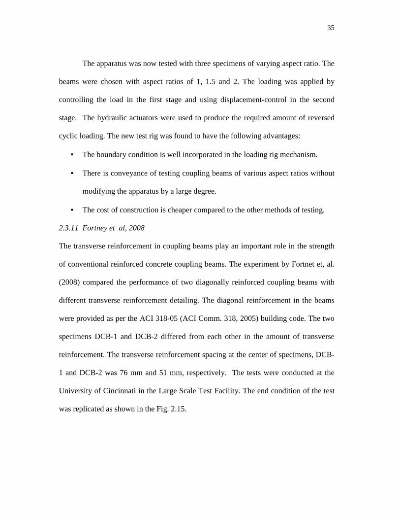
was replicated as shown in the Fig. 2.15.

36

Fig. 2.15. Testing Setup of Coupling Beam Specimen (Fortney et al., 2008)

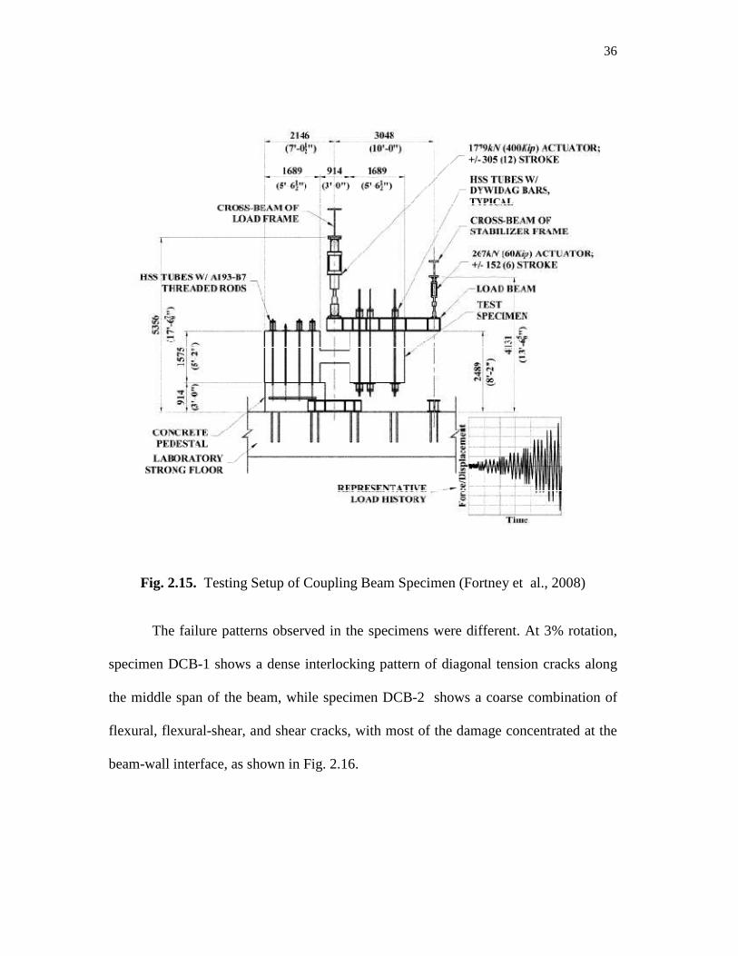
The failure patterns observed in the specimens were different. At 3% rotation,

specimen DCB-1 shows a dense interlocking pattern of diagonal tension cracks along

the middle span of the beam, while specimen DCB-2 shows a coarse combination of

flexural, flexural-shear, and shear cracks, with most of the damage concentrated at the

beam-wall interface, as shown in Fig. 2.16.

37

Fig. 2.16. Cracking Pattern Observed at 3% Chord Rotation (Fortney et al., 2008)

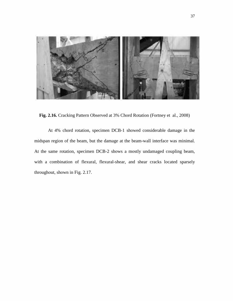
At 4% chord rotation, specimen DCB-1 showed considerable damage in the

midspan region of the beam, but the damage at the beam-wall interface was minimal.

At the same rotation, specimen DCB-2 shows a mostly undamaged coupling beam,

with a combination of flexural, flexural-shear, and shear cracks located sparsely

throughout, shown in Fig. 2.17.

38

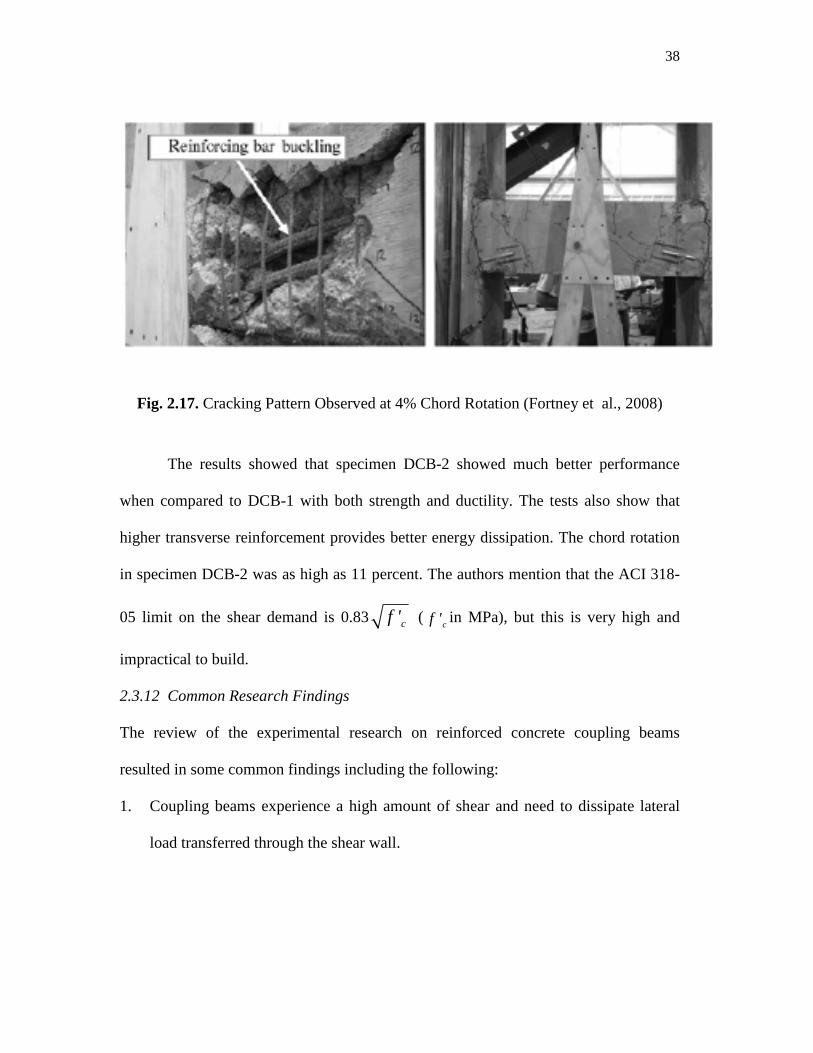
Fig. 2.17. Cracking Pattern Observed at 4% Chord Rotation (Fortney et al., 2008)

The results showed that specimen DCB-2 showed much better performance

when compared to DCB-1 with both strength and ductility. The tests also show that

higher transverse reinforcement provides better energy dissipation. The chord rotation

in specimen DCB-2 was as high as 11 percent. The authors mention that the ACI 318-

05 limit on the shear demand is 0.83 cf ' (cf ' in MPa), but this is very high and

impractical to build.

2.3.12 Common Research Findings

The review of the experimental research on reinforced concrete coupling beams

resulted in some common findings including the following:

1. Coupling beams experience a high amount of shear and need to dissipate lateral

load transferred through the shear wall.

39

2. Conventionally reinforced coupling beams experience high shear at the joint of the

connection between shear walls. The shear is resisted by providing a large amount

of transverse reinforcement.

3. Diagonally reinforced coupling beams resist shear force by truss action developed

in the diagonal reinforcement and perform better when compared as conventional

reinforced coupling beams as seen in Paulay and Binney (1974) and Galano and

Vignoli (2000).

4. An optimum aspect ratio range is between 2 to 3 for efficient performance as

observed by Barney et al. (1980) and Tassios et al. (1996) .

2.4 Analytical Research

Simulating the behavior of coupling beams in the laboratory is costly, and poses a

difficulty in replicating the actual end-conditions and the seismic loading. Analytical

research aims to overcome some of these limitations. The properties and the behavior

of the materials need to be replicated under the right loading and boundary conditions.

While a number of analytical models have been developed, finite element models are

frequently used to simulate behavior.

2.4.1 Paulay, 1970

The elasto-plastic behavior of coupling beams is captured in the model proposed by

Paulay (1970). His paper introduces the shortfalls of laminar theory for analyzing

coupling beams and then introduces a new methodology to overcome these limitations.

The laminar method, which considers the effect of change in stiffness due to cracking,

does not reflect the nature of coupled shear walls system. Therefore, cracking need not

40

significantly affect the behavior of the bending moment pattern in the frame. The

following steps are performed for analyzing the beam using the proposed method:

• The static design load and the lateral deflection are assumed.

• The rotational ductility is calculated (Ө/ Өy).

• The load stage which brings about yielding is selected marking the end of the

linear elastic behavior.

• Incrementing the load further will cause coupling beams to enter the plastic

range. It is assumed that the laminas possess bilinear elasto-plastic load rotation

characteristics. At the end of this load, the laminar plasticization is assumed to

have spread over the height of the structure while each beam sustains its yield

capacity.

• The ultimate axial tension or compression in the walls can be conservatively estimated

by

0.u uT 95q H≥ (2.1)

where qu is the ultimate shear capacity of the lamina and H is the height of the

building.

• The moments at the top of the walls and the shear rotation are estimated.

• The load at which these moments occur is estimated.

• A further load increment W' may be assumed to cause Wall 1 to attain its

ultimate capacity in the presence of T" axial tension. The critical moment at the

base of the wall is obtained.

41

• Superimposing the previous load increments, the ultimate triangular load

intensity is obtained.

• When the load-deflection relationship is approximated by a bilinear relation. It

may be said that the attainment of the ultimate load is characterized by an over-

all ductility factor of two.

The authors conclude by stating that the laminar analysis can be extended to

predict the elastic behavior of coupled shear walls at various stages of cracking by

accounting for the loss of stiffness in the components. The changes to the critical

moment can occur due to cracking and can be analyzed using a step by step procedure

which includes the effect of post elastic behavior.

2.4.2 Zhao et al., 2004

Zhao et al. (2004) used the smeared crack model for the simulation of the coupling

beams based on the experimental work conducted by Kwan and Zhao (2002). The

model assumed a plane stress formulation for modeling concrete and the steel

reinforcement. The steel was assumed to be perfectly bonded with the concrete. At

each incremental load–displacement step, direct iteration using the secant stiffness of

the structure was employed so that the analysis could be extended into the post-peak

range within which the tangent stiffness can become zero or negative. The model was

able to accurately simulate the experimental results with reasonable tolerances.

Although the model performed well with the end conditions prescribed in the

experiment, it was not tested against different end conditions or loading patterns. The

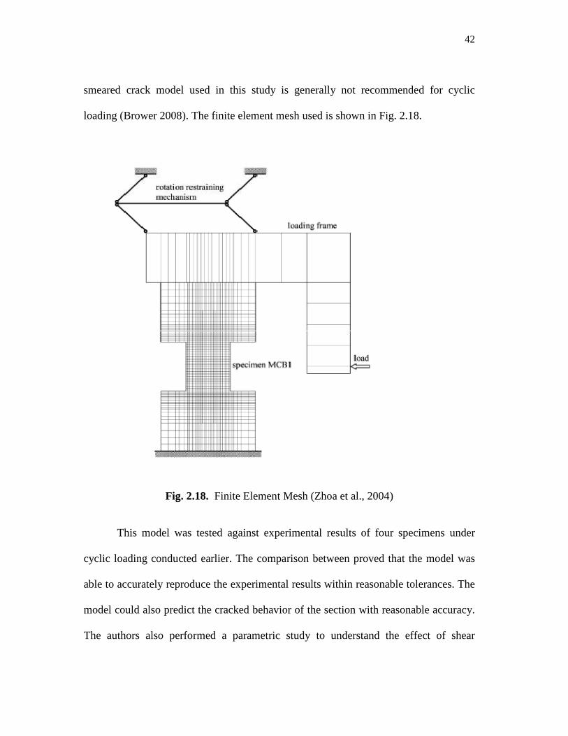
42

smeared crack model used in this study is generally not recommended for cyclic

loading (Brower 2008). The finite element mesh used is shown in Fig. 2.18.

Fig. 2.18. Finite Element Mesh (Zhoa et al., 2004)

This model was tested against experimental results of four specimens under

cyclic loading conducted earlier. The comparison between proved that the model was

able to accurately reproduce the experimental results within reasonable tolerances. The

model could also predict the cracked behavior of the section with reasonable accuracy.

The authors also performed a parametric study to understand the effect of shear

43

reinforcement and end conditions on the results. They found that the rate of

improvement of shear strength with respect to the amount of shear reinforcement

reduces and that axial elongation plays a significant role in the behavior of the coupling

beam.

2.4.3 Hindi and Hassan, 2007

Hindi and Hassan (2007) proposed a model making the following assumptions. The

monotonic force-displacement relationship of the diagonally reinforced coupling beam

was assumed to be linear up to the yield strain of the diagonal reinforcement. The

unconfined concrete was assumed to reach it maximum unconfined compressive

strength, which was taken to be equal to the 28-day strength, f'c. The confined concrete

behavior was characterized by the model proposed by Mander et al. (1988). The yield

shear force Vy of the diagonally reinforced coupling beam was expressed as

( )y y yV T C sinα= + (2.2)

y s yT A f= (2.3)

( ' )y s y c cC A f A f= − (2.4)

where Ty and Cy are the yield diagonal tensile and compressive forces, respectively; fy

is the yield strength of the diagonal reinforcement; As is the area of diagonal

reinforcement in the considered direction; Ac is the area of the concrete core within the

diagonal; and α is the angle between the diagonal reinforcement. This model proved

effective in reproducing the monotonic behavior of diagonally reinforced coupling

beams from various experiments. The model was able to predict the backbone curve for

the experiments where the coupling beams were subjected to cyclic loading. However,

44

the validity of the model was not tested for cyclic loading, which is essential for proper

understanding of the behavior of the coupling beam.

The model was compared with experimental results for validation. The model

was compared to the four test beams by Pauley and Binney (1974) and fifteen test

beams used by Galano and Vignoli (2000). The comparison of the ultimate shear

capacities obtained from experimental results, the analytical solutions proposed by

Paulay (1970) and Galano and Vignoli (2000) and the results obtained by the proposed

trilinear model are as shown in the Table 2.3. The authors concluded that the proposed

model is in good agreement with the experimental results for beams with an aspect

ratio ranging from 1.0 to 2.74. The model is seen to provide a good estimate of the

behavior of the coupling beams, having a mean value ratio of the proposed to the

experimental shear strength of 0.98 with a standard deviation of 0.08

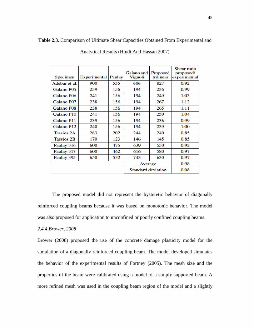
Table 2.3. Comparison of Ultimate Shear Capacities Obtained From Experimental

Analytical Results (Hindi And Hassan 2007)

The proposed model did

reinforced coupling beams because it was based on monotonic behavior. The model

was also proposed for application

2.4.4 Brower, 2008

Brower (2008) proposed the use of the concrete damage plasticity model

simulation of a diagonally reinforced coupling beam

the behavior of the experimental results of Fortney (2005). The mesh size and the

properties of the beam were calibr

more refined mesh was used in the coupling beam region

Ultimate Shear Capacities Obtained From Experimental

Analytical Results (Hindi And Hassan 2007)

l did not represent the hysteretic behavior of diagonally


was also proposed for application to unconfined or poorly confined coupling beams.

the use of the concrete damage plasticity model

simulation of a diagonally reinforced coupling beam. The model developed simulates


properties of the beam were calibrated using a model of a simply supported beam.

was used in the coupling beam region of the model and a slightly

45

Ultimate Shear Capacities Obtained From Experimental and

not represent the hysteretic behavior of diagonally


to unconfined or poorly confined coupling beams.

the use of the concrete damage plasticity model for the

. The model developed simulates


ated using a model of a simply supported beam. A

of the model and a slightly

46

coarser mesh for the shear wall region. Though the selected model parameters could

replicate the simply supported beam well, they did not have the same accuracy for

predicting the behavior of the coupling beam. The model also failed to account for the

evolution of the damage parameters, the tension stiffening of concrete, and the plastic

behavior of the steel reinforcement.

2.5 Research Needs

Based on the literature review, there is a need for a more versatile model that can

replicate the behavior of the coupling beams with varying boundary conditions and also

simulate the cyclic performance of coupling beam. The focus of this research is to investigate

the use of finite element modeling techniques to predict the behavior of conventionally

concrete reinforced coupling beams.

47

3. FINITE ELEMENT MODELING

3.1 Introduction

This section details the modeling procedure used for this study. The use of finite

elements in simulating behavior of structural elements is a common practice. This is

done in this case with the help of a commercial package ABAQUS (ABAQUS 2008).

ABAQUS is a powerful numerical tool used for component and system modeling and

finds it application in various fields. It is used to solve multi-degree and multi-physics

transient problems. ABAQUS has several built-in models to predict the behavior of

materials as well as the provision to add user defined models. The response of concrete

can be modeled with the help of two built-in models in ABAQUS: the concrete

damaged plasticity model and the smeared concrete model. Descriptions of both of

these models have been made in subsequent sections.

3.2 Finite Element Method of Analysis

The finite element method is a numerical method for solving differential equations. It

finds its applications in solving spatial and temporal distribution of one or more

variables in field problems. They are usually solved by discretization the geometry

over which the problem needs to be solved into nodes. These nodes are connected to

form elements. The collection of the elements and nodes is called the mesh. After

applying appropriate initial and boundary conditions, the problem is solved as a

differential equation at each of these nodes based on the formulation of the problem.

48

Individual finite elements can be visualized as small parts of the geometry. In

each of these elements a field quantity is allowed to have a simple spatial variation.

However, when combined for a region this becomes more complicated and therefore

results in an approximate solution. The field quantity to be determined is numerically

represented using differential equations at each node that are solved and later

assembled over the entire geometry. The size, shape, location and the element type all

have an influence on the solution. The solution generally improves with the refinement

in the mesh and converges to a unique solution. This, however, is not true in all cases

as excess refinement introduces error due to round off and redundancy. The excessive

refinement also increases the runtime of the problem, which is not desirable. The most

desirable mesh size is one that simulates the actual problem with the least runtime and

is called the optimum mesh size. The optimum mesh size is obtained by conducting a

mesh refinement study.

3.3 Material Models

Accurate simulation through a computational effort requires the properties of the

materials involved to be modeled as close to the physical specimen as possible.

Therefore, the material models in this study are required to describe the inelastic

behavior of concrete and steel. The Mander model developed by Mander et al. (1988)

is chosen as the analytical model to simulate the behavior of concrete. This constitutive

model is based on the Popovics equation (Popovics 1973) so as to incorporate the

effect of confinement. This model has been verified both analytical and experimentally

by Mander et al. (1988) and Mander and Priestley (1988). The tensile stress-strain

49

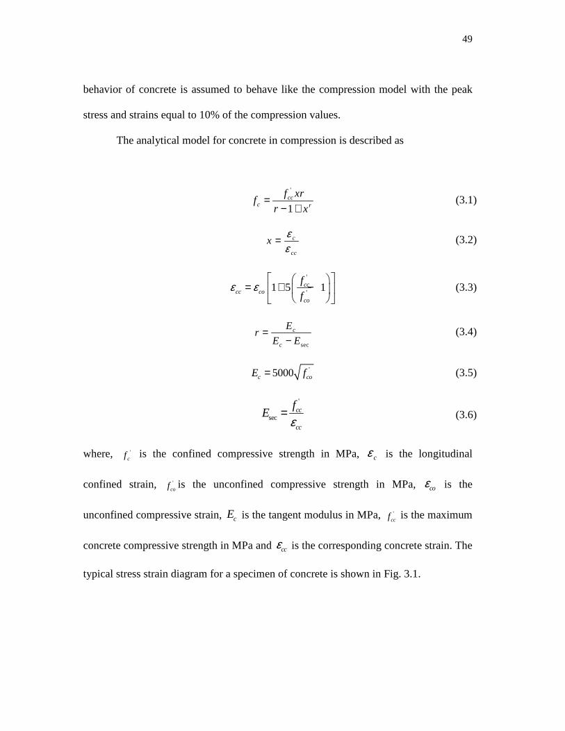
behavior of concrete is assumed to behave like the compression model with the peak

stress and strains equal to 10% of the compression values.

The analytical model for concrete in compression is described as

'

1cc

c r

f xrf

r x=

− + (3.1)

c

cc

xεε

= (3.2)

'

'1 5 1cc

cc coco

f

fε ε

= + −

(3.3)

sec

c

c

Er

E E=

− (3.4)

'5000c coE f= (3.5)

'

seccc

cc

fE

ε= (3.6)

where, ' cf is the confined compressive strength in MPa, cε is the longitudinal

confined strain, 'cof is the unconfined compressive strength in MPa, coε is the

unconfined compressive strain, cE is the tangent modulus in MPa, ' ccf is the maximum

concrete compressive strength in MPa and ccε is the corresponding concrete strain. The

typical stress strain diagram for a specimen of concrete is shown in Fig. 3.1.

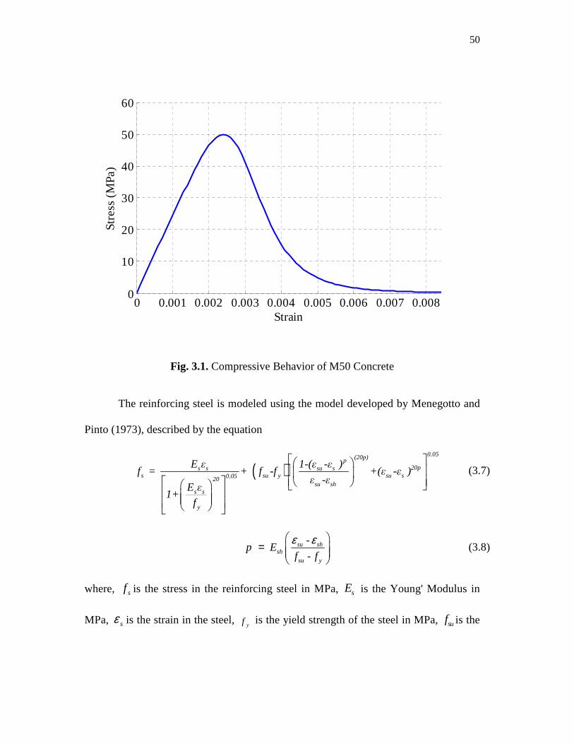
50

Fig. 3.1. Compressive Behavior of M50 Concrete

The reinforcing steel is modeled using the model developed by Menegotto and

Pinto (1973), described by the equation

( )0.05(20p)p

20ps s su ss su y su s0.0520

su shs s

y

E ε 1-(ε -ε )f = + f -f +( ε -ε )

ε -εE ε

1+f

(3.7)

-

-

su shsh

su y

p Ef f

ε ε =

(3.8)

where, sf is the stress in the reinforcing steel in MPa, sE is the Young' Modulus in

MPa, sε is the strain in the steel, yf is the yield strength of the steel in MPa, suf is the

0 0.001 0.002 0.003 0.004 0.005 0.006 0.007 0.0080

10

20

30

40

50

60

Strain

Str

ess

(M

Pa

)

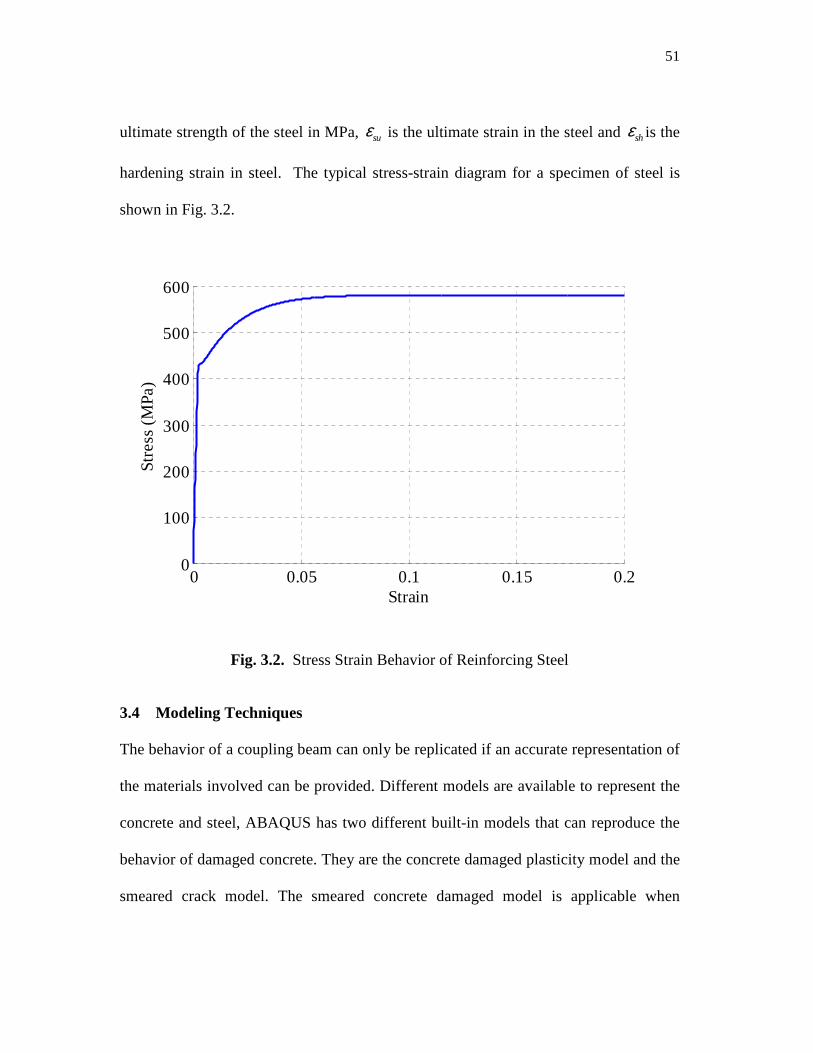
51

ultimate strength of the steel in MPa, suε is the ultimate strain in the steel and shε is the

hardening strain in steel. The typical stress-strain diagram for a specimen of steel is

shown in Fig. 3.2.

Fig. 3.2. Stress Strain Behavior of Reinforcing Steel

3.4 Modeling Techniques

The behavior of a coupling beam can only be replicated if an accurate representation of

the materials involved can be provided. Different models are available to represent the

concrete and steel, ABAQUS has two different built-in models that can reproduce the

behavior of damaged concrete. They are the concrete damaged plasticity model and the

smeared crack model. The smeared concrete damaged model is applicable when

0 0.05 0.1 0.15 0.20

100

200

300

400

500

600

Strain

Str

ess

(M

Pa

)

52

concrete is subjected essentially to monotonic loading either in tension or compression

(Bower 2008). Failure is characterized as cracking in tension or crushing of concrete in

compression. The experimental data used in this study has loading that is cyclic in

nature. Therefore, the concrete model should accommodate the corresponding actions

such as recovery of stiffness on reversal of loading and cracked behavior of concrete.

The concrete damaged plasticity model is seen as the best option to do this as it

incooperates these characteristics. A description of the formulation and assumptions

made in the concrete damaged plasticity model is presented below.

3.4.1 Concrete Damaged Plasticity Model

The concrete damaged plasticity model is based on the plasticity model proposed by

Lubliner et al. (1989) and by Lee and Fenves (1998).The salient features of model are

discussed here.

This model is assumed to be an inviscid concrete damage model. An additive

strain rate is assumed

e pij ij ijε ε ε= +& & & (3.9)

where, ijε& is the additive strain rate, eijε& is the elastic strain rate and pijε& is the plastic

strain rate.

The stress-strain relation is governed by scalar damaged elasticity as follows

0(1- ) ( - )el pij ijkl kl kld Dσ ε ε= (3.10)

where, ijσ is the stress in concrete in MPa, 0

elijklD is the initial (undamaged) stiffness of

the material in MPa and d is the scalar stiffness degradation variable klε and pklε are

53

the total and plastic strains, respectively. The hardening variables are characterized

independently for compression and tension by taking the variables and,ij

pttε% and

ij

pcε%

which are the equivalent strains in tension and compression respectively. The evolution

of the variables ij

pttε% and

ij

pcε% are formulated to uniaxial loading conditions first and

extended later to multiaxial conditions.

For uniaxial loading conditions the following assumptions are made. The stress-

strain curves can be converted into stress versus plastic strain by consideration of the

following equations

( , , , )ij ij ij ij

p pt t tt tt ifσ σ ε ε θ= &% % (3.11)

( , , , )ij ij ij ij

p pc c c c ifσ σ ε ε θ= &% % (3.12)

where, θ is the temperature and �� accounts for other predefined variables. Here the

subscripts of t and c refer to tension and compression, respectively. The equivalent

plastic strains are given by the equations

0

ij ij

tp pc cε ε= ∫ &% % (3.13)

0

ij ij

tp pt tε ε= ∫ &% % (3.14)

Under uniaxial loading the strain rates in tension and compression respectively are

11

11

ij

ij

p pt t

p pc c

ε ε

ε ε

=

=

& &% %

& &% %

(3.15)

When the concrete specimen is unloaded from any point on the stress

curve, the unloading response is observed to be weakened. The

degraded and this is characterized by age variables

compression respectively assumed to be functions of plastic strains, temperatures and

field variables:

The stress-strain behavior in tension and compression obtained using the above

formulation is shown in Fig.

Fig. 3.3. Concrete Behavior in Tension (ABAQUS

When the concrete specimen is unloaded from any point on the stress

curve, the unloading response is observed to be weakened. The stiffness is said to have

degraded and this is characterized by age variables dt and dc for tension and


( , , ) (0 1)ij

pt t i ttd d f d= ε θ ≤ ≤%

( , , ) (0 1)ij

pc c i ccd d f d= ε θ ≤ ≤%

strain behavior in tension and compression obtained using the above

3.3 and Fig. 3.4, respectively.

Concrete Behavior in Tension (ABAQUS 2008)

54

When the concrete specimen is unloaded from any point on the stress-stain

stiffness is said to have

for tension and


(3.16)

(3.17)

strain behavior in tension and compression obtained using the above

Fig. 3.4. Concrete Behavior in Compression

If 0ijklE is the initial (undamaged) elastic stiffness of the material the stress

strain relationship is

Under uniaxial loading cracks propagate in a direction normal to the direction

of stress. The nucleation and propagation of cracks, therefore causes a reduction of the

available load carrying area, there

uniaxial cohesion stresses, which determine the size of the yield surface

σ = σ − = ε − ε% %

σ = σ − = ε − ε% %

Concrete Behavior in Compression (ABAQUS 2008)

is the initial (undamaged) elastic stiffness of the material the stress

( ) 01 ( )ij ijkl ij ij

ptt t td Eσ = − ε − ε%

( ) 01 ( )ij ijkl ij ijcp

c ccd Eσ = − ε − ε%



available load carrying area, therefore increasing the effective stress. The effective

which determine the size of the yield surface are given by

( ) 01/ ( )ijkl ij ijij ij

pt t tt t d Eσ = σ − = ε − ε%% %

( ) 01/ ( )ijkl ij ii jj i jcp

c c cc d Eσ = σ − = ε − ε%% %

55

is the initial (undamaged) elastic stiffness of the material the stress

(3.18)

(3.19)



fore increasing the effective stress. The effective

given by

(3.20)

(3.21)

56

Under uniaxial cyclic loading the degradation behavior involves the opening

and closing of previously formed micro-cracks. It is observed through experiments that

there is a recovery of elastic stiffness as the load changes, this effect is called

"unilateral effect." This effect is seen in a greater degree when the load changes from

tension to compression. The elastic modulus of the material is expressed in terms of the

scalar degradation as

0(1 ) ijk li jk lE d E= − (3.22)

where, 0 ijklE is the initial (undamaged) modulus of the material.

This expression holds both in tensile and compressive sides of the cycle. The

stiffness reduction variable and the damage variabletd and cd are assumed as,

(1 ) (1 )(1 ) 0 , 1t t c c t cd s d s d s s− = − − ≤ ≤ (3.23)

where, �� and �� are functions of the stress state and are introduced to represent

stiffness recovery effects defined as

*111 ( ) 0 1t t ts w r w= − σ ≤ ≤ (3.24)

*111 (1 ( )) 0 1c c cs w r w= − − σ ≤ ≤ (3.25)

where,

11*

1111

01( )

00{ if

rif

σ >σ =

σ ≤ (3.26)

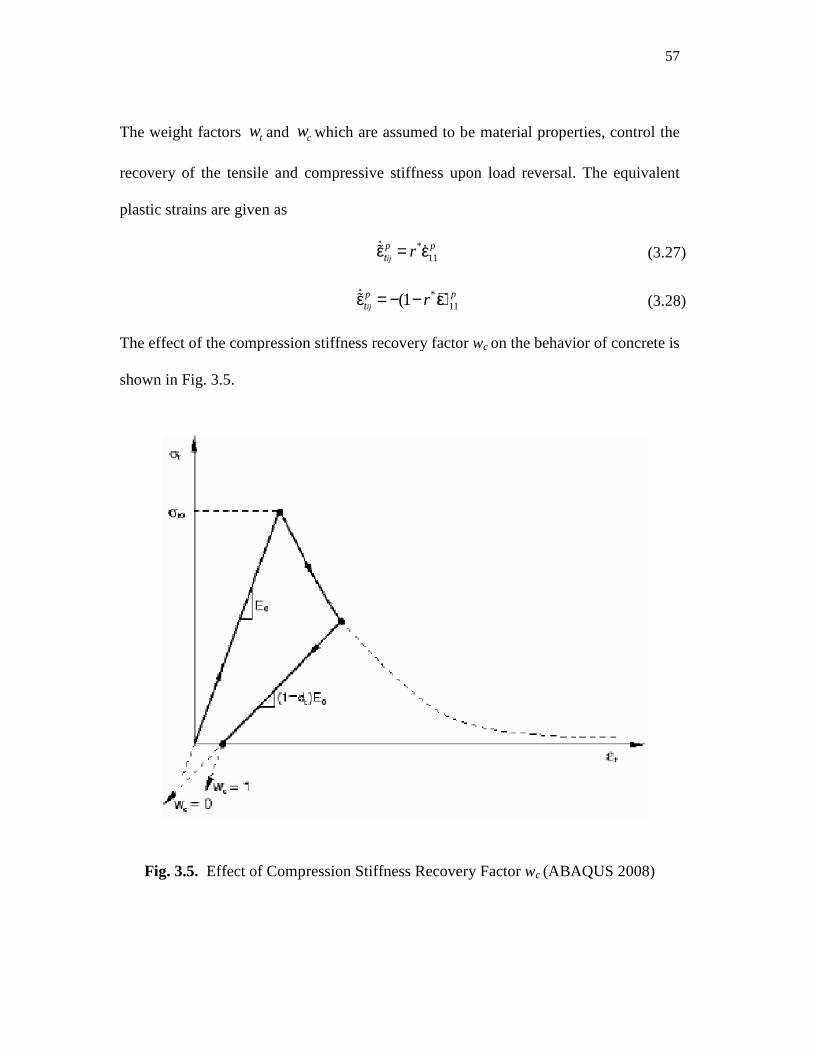
The weight factors tw and w

recovery of the tensile and compressive stiffness upon load reversal.

plastic strains are given as

The effect of the compression stiffness recovery factor

shown in Fig. 3.5.

Fig. 3.5. Effect of Compress

cw which are assumed to be material properties, control the

recovery of the tensile and compressive stiffness upon load reversal. The equivalent

*11ij

p pt rε = ε&% &

*11(1ij

p pt rε = − − )ε&% &

The effect of the compression stiffness recovery factor wc on the behavior of concrete is

Effect of Compression Stiffness Recovery Factor wc (ABAQUS 2008)

57

which are assumed to be material properties, control the

The equivalent

(3.27)

(3.28)

on the behavior of concrete is

(ABAQUS 2008)

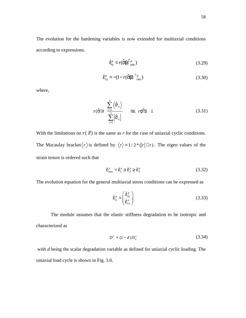
58

The evolution for the hardening variables is now extended for multiaxial conditions

according to expressions.

maxˆˆ( )ij

p pt rε = σ)(ε&% & (3.29)

minˆˆ(1 ( )ij

p pc rε = − − σ))(ε&% & (3.30)

where,

3

13

1

ˆˆ ˆ( 0 ( 1

ˆ

iii

iii

r r=

=

σσ) = ≤ σ) ≤

σ

∑

∑

(3.31)

With the limitations on �� is the same as r for the case of uniaxial cyclic conditions.

The Macaulay bracketr is defined by 1 / 2 * ( )r r r= + . The eigen values of the

strain tensor is ordered such that

max 1 2 3p p p pε = ε ≥ ε ≥ ε& & & &% % % % (3.32)

The evolution equation for the general multiaxial stress conditions can be expressed as

ij

ij

ppij p

t

c

εε = ε

&%&%

&% (3.33)

The module assumes that the elastic stiffness degradation to be isotropic and

characterized as

0(1 )e eD d D= − (3.34)

with d being the scalar degradation variable as defined for uniaxial cyclic loading. The

uniaxial load cycle is shown in Fig. 3.6.

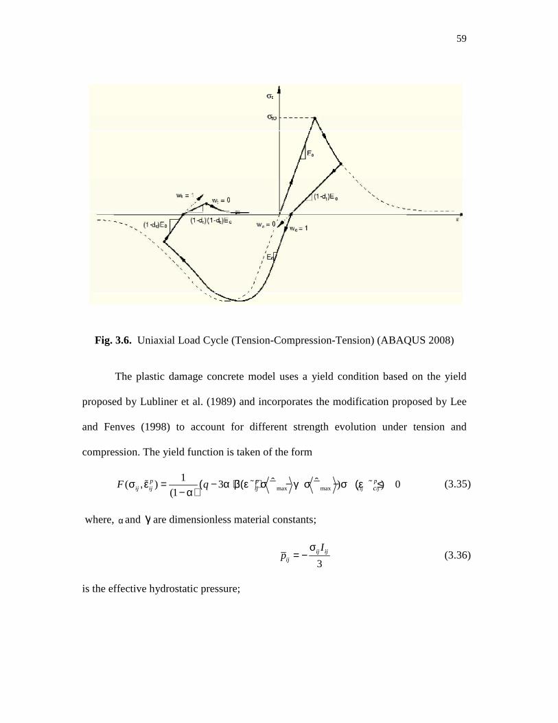
59

Fig. 3.6. Uniaxial Load Cycle (Tension-Compression-Tension) (ABAQUS 2008)

The plastic damage concrete model uses a yield condition based on the yield

proposed by Lubliner et al. (1989) and incorporates the modification proposed by Lee

and Fenves (1998) to account for different strength evolution under tension and

compression. The yield function is taken of the form

max max

1 ˆ ˆ( ) 3 ) ) 0(1 ij ij

p p pij ij ij c cF qσ ,ε = ( − α + β(ε ) σ − γ σ − σ (ε ≤

− α)% % % (3.35)

where, αand γ are dimensionless material constants;

3ij ij

ij

Ip

σ= − (3.36)

is the effective hydrostatic pressure;

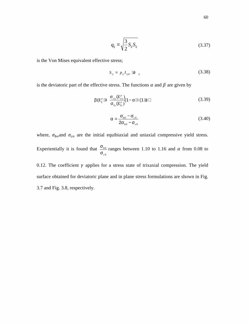
60

3

2ij ij ijq S S= (3.37)

is the Von Mises equivalent effective stress;

i j i j i jk l ijS p I= + σ (3.38)

is the deviatoric part of the effective stress. The functions � and � are given by

)

)ij ij

ij ij

ppij p

c c

t t

σ (εβ(ε ) = (1 − α) − (1 + α)

σ (ε%

%%

(3.39)

0 0

0 0

b c

b c

σ − σα =2σ − σ

(3.40)

where, ��and �� are the initial equibiaxial and uniaxial compressive yield stress.

Experientially it is found that 0

0

b

c

σσ

ranges between 1.10 to 1.16 and � from 0.08 to

0.12. The coefficient applies for a stress state of trixaxial compression. The yield

surface obtained for deviatoric plane and in plane stress formulations are shown in Fig.

3.7 and Fig. 3.8, respectively.

61

Fig. 3.7. Yield Surface of Deviatoric Plane (ABAQUS 2008)

Fig. 3.8. Yield Surface in Plane Stress (ABAQUS 2008).

62

The plastic-damage model assumes non-associated potential flow,

( )ijp

ijij

Gδδ

σε = λ

σ&& (3.41)

The flow potential G chosen for this model is the Drucker-Prager hyperbolic function:

2 20 tan ) tan

ij ij ijtG q p= (ξσ ψ + − ψ (3.42)

where, is the dilation angle measure in the p-q plane at high confining pressure; ��

is the uniaxial tensile stress at failure; and ξ is the eccentricity that defines the rate at

which the function approaches the asymptote value.

3.4.2 Selected Model Parameters

ABAQUS requires the following input for computing the damage in concrete:

• Dilation angle, ψ

• Flow potential eccentricity, ε . The default of ε =0.1 is used.

• 0 0b cσ σ is the ratio of initial equibiaxial compressive yield stress to initial

uniaxial compressive yield stress. The default of 1.16 is used.

• cK , the ratio of the second stress invariant on the tensile meridian, q(TM), to

that on the compressive meridian, q(TM) . The default of 2/3 is used.

• Viscosity parameter, µ , used for the visco-plastic regularization of the

concrete constitutive equations in ABAQUS Standard analyses. The default

value is 0.0. (°C).

63

3.5 Element Type

ABAQUS has a wide variety of elements that can be used and it is important to select

the right element based on the problem. The coupling beams here are modeled in two

dimensions for which the concrete is modeled using solid elements. The solid elements

are provided with the appropriate thickness based on the experimental specimen

dimension. The reinforcement can be modeled using solid, beam or truss elements. The

use of solid elements is computationally expensive and therefore not chosen. Because

the reinforcing bars do not provide a very high bending stiffness, truss elements are

used. Because the reinforcement is a two dimensional wire it can only be modeled as

an embedded element and its contact with the concrete is assumed to be perfectly

bonded. The slip of the reinforcement can be modeled by modifying the behavior of

concrete. This, however, is not studied here.

The model is analyzed as a plane stress problem where the change in stress in

the direction of the thickness is ignored. Second order elements are chosen as they

provide higher accuracy for elements with severe distortions, they capture stress

concentrations better, and are effective in bending dominated problems. Full

integration with second order elements are preferred as they yield more accurate

results. This combination of full integration with second order elements also prevent

problems with shear locking and hourglassing as large strains are expected. Therefore

the CPS8 (eight-noded plane stress quadrilateral with full integration) elements are

chosen to the model concrete, and T2D3 (3-noded quadratic 2-D truss) elements are

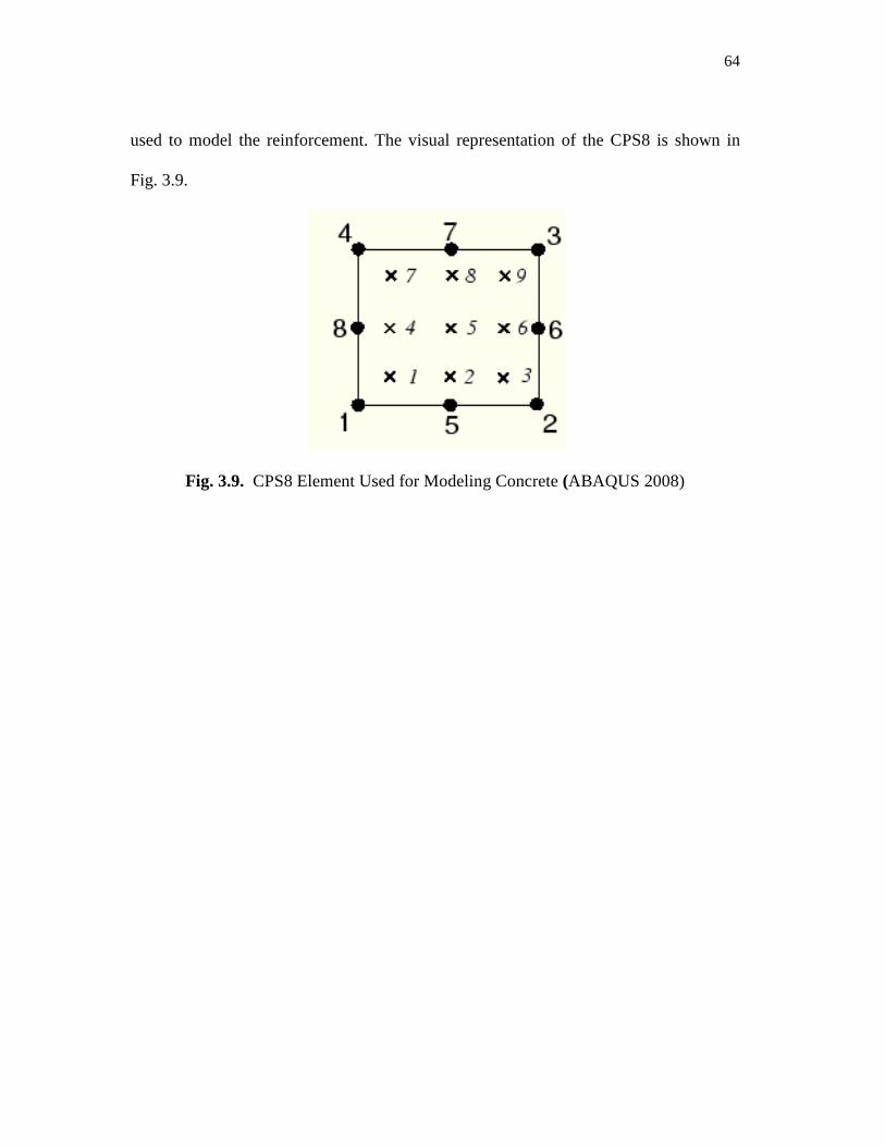
64

used to model the reinforcement. The visual representation of the CPS8 is shown in

Fig. 3.9.

Fig. 3.9. CPS8 Element Used for Modeling Concrete (ABAQUS 2008)

65

4. CALIBRATION MODEL

4.1 Introduction

A calibration model was prepared prior to simulating the coupling beams to better

understand the effects of several modeling parameters. The response of a simple

cantilever beam was analyzed in RESPONSE 2000 (Bentz 2000) and then compared

with results of an ABAQUS model. The description of the cantilever beam and results

obtained are discussed below.

4.2 RESPONSE 2000 Modeling

RESPONSE 2000 is a reinforced concrete analysis program based on the modified

compression field theory, and was used as a benchmarking tool for calibrating the

parameters used in the ABAQUS model. RESPONSE 2000 is a simple tool to analyze

the behavior of concrete sections. As part of this study, RESPONSE 2000 was used to

obtain the force deflection and moment curvature behavior of a simple cantilever beam.

The detailed stress strain behavior of steel and concrete can be described in the material

properties section of the program. The proper end conditions and loading parameters

are provided in the load section of the program. The results obtained in this study are

discussed in the following sections.

4.3 Cantilever Model

The selected cantilever beam is 3 m long with cross section dimensions of 400 mm X

150 mm. This section was chosen specifically to as beam which would be subjected to

high amount of bending. Therefore the length of the beam was 3 m. The section was

kept in accordance with the coupling beam to be modeled. The section was doubly

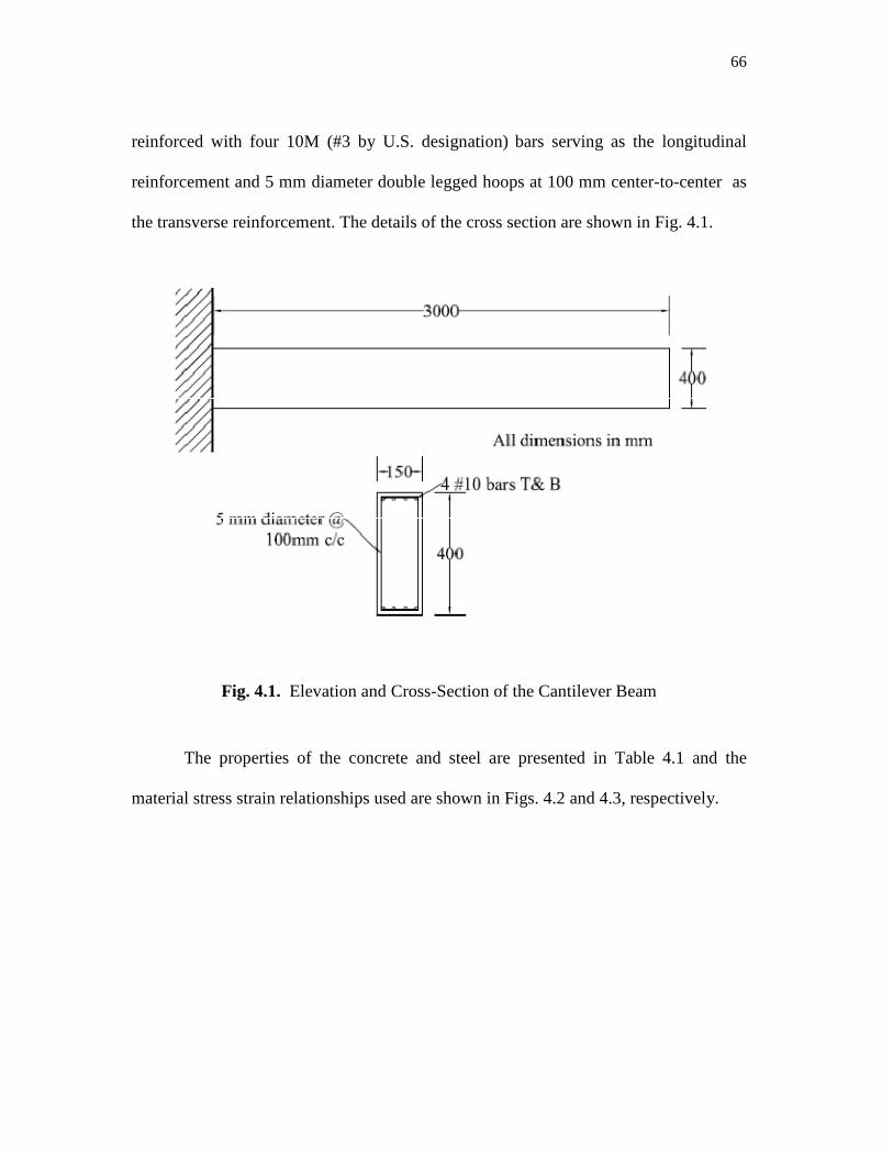
66

reinforced with four 10M (#3 by U.S. designation) bars serving as the longitudinal

reinforcement and 5 mm diameter double legged hoops at 100 mm center-to-center as

the transverse reinforcement. The details of the cross section are shown in Fig. 4.1.

Fig. 4.1. Elevation and Cross-Section of the Cantilever Beam

The properties of the concrete and steel are presented in Table 4.1 and the

material stress strain relationships used are shown in Figs. 4.2 and 4.3, respectively.

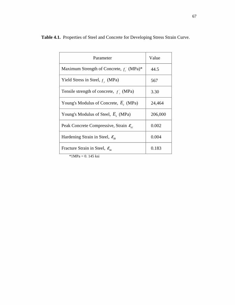
67

Table 4.1. Properties of Steel and Concrete for Developing Stress Strain Curve.

Parameter Value

Maximum Strength of Concrete,' cf (MPa)* 44.5

Yield Stress in Steel,yf (MPa) 567

Tensile strength of concrete, 'tf (MPa) 3.30

Young's Modulus of Concrete, cE (MPa) 24,464

Young's Modulus of Steel, sE (MPa) 206,000

Peak Concrete Compressive, Strain ccε 0.002

Hardening Strain in Steel, shε 0.004

Fracture Strain in Steel, suε 0.183

*1MPa = 0. 145 ksi

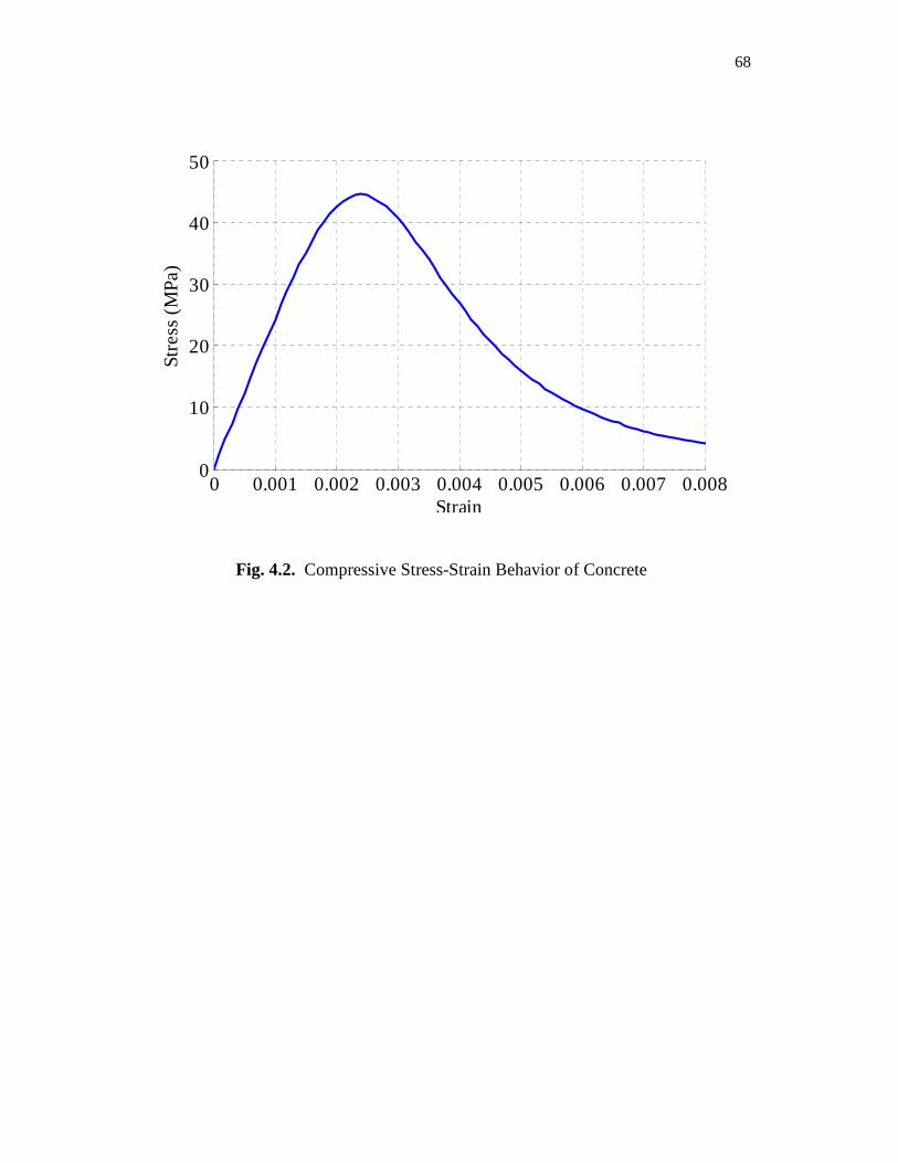
68

Fig. 4.2. Compressive Stress-Strain Behavior of Concrete

0 0.001 0.002 0.003 0.004 0.005 0.006 0.007 0.0080

10

20

30

40

50

Strain

Str

ess

(M

Pa

)

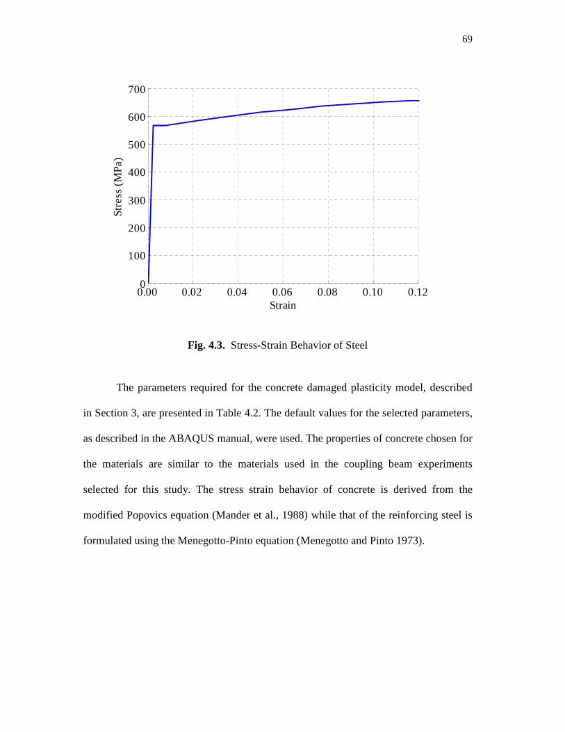
69

Fig. 4.3. Stress-Strain Behavior of Steel

The parameters required for the concrete damaged plasticity model, described

in Section 3, are presented in Table 4.2. The default values for the selected parameters,

as described in the ABAQUS manual, were used. The properties of concrete chosen for

the materials are similar to the materials used in the coupling beam experiments

selected for this study. The stress strain behavior of concrete is derived from the

modified Popovics equation (Mander et al., 1988) while that of the reinforcing steel is

formulated using the Menegotto-Pinto equation (Menegotto and Pinto 1973).

0.00 0.02 0.04 0.06 0.08 0.10 0.12 0

100

200

300

400

500

600

700

Strain

Str

ess

(M

Pa

)

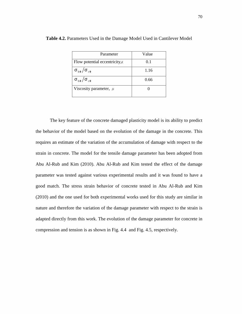
70

Table 4.2. Parameters Used in the Damage Model Used in Cantilever Model

Parameter Value

Flow potential eccentricity,ϵ 0.1

b c0 0σ σ 1.16

b c0 0σ σ 0.66

Viscosity parameter, μ 0

The key feature of the concrete damaged plasticity model is its ability to predict

the behavior of the model based on the evolution of the damage in the concrete. This

requires an estimate of the variation of the accumulation of damage with respect to the

strain in concrete. The model for the tensile damage parameter has been adopted from

Abu Al-Rub and Kim (2010). Abu Al-Rub and Kim tested the effect of the damage

parameter was tested against various experimental results and it was found to have a

good match. The stress strain behavior of concrete tested in Abu Al-Rub and Kim

(2010) and the one used for both experimental works used for this study are similar in

nature and therefore the variation of the damage parameter with respect to the strain is

adapted directly from this work. The evolution of the damage parameter for concrete in

compression and tension is as shown in Fig. 4.4 and Fig. 4.5, respectively.

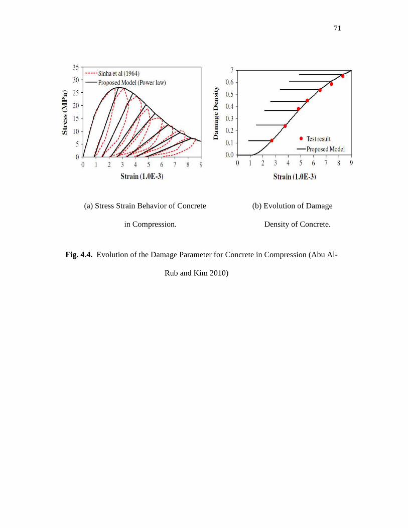
71

(a) Stress Strain Behavior of Concrete (b) Evolution of Damage

in Compression. Density of Concrete.

Fig. 4.4. Evolution of the Damage Parameter for Concrete in Compression (Abu Al-

Rub and Kim 2010)

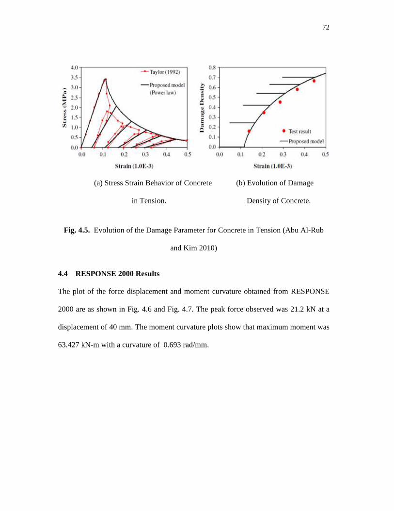
72

(a) Stress Strain Behavior of Concrete (b) Evolution of Damage

in Tension. Density of Concrete.

Fig. 4.5. Evolution of the Damage Parameter for Concrete in Tension (Abu Al-Rub

and Kim 2010)

4.4 RESPONSE 2000 Results

The plot of the force displacement and moment curvature obtained from RESPONSE

2000 are as shown in Fig. 4.6 and Fig. 4.7. The peak force observed was 21.2 kN at a

displacement of 40 mm. The moment curvature plots show that maximum moment was

63.427 kN-m with a curvature of 0.693 rad/mm.

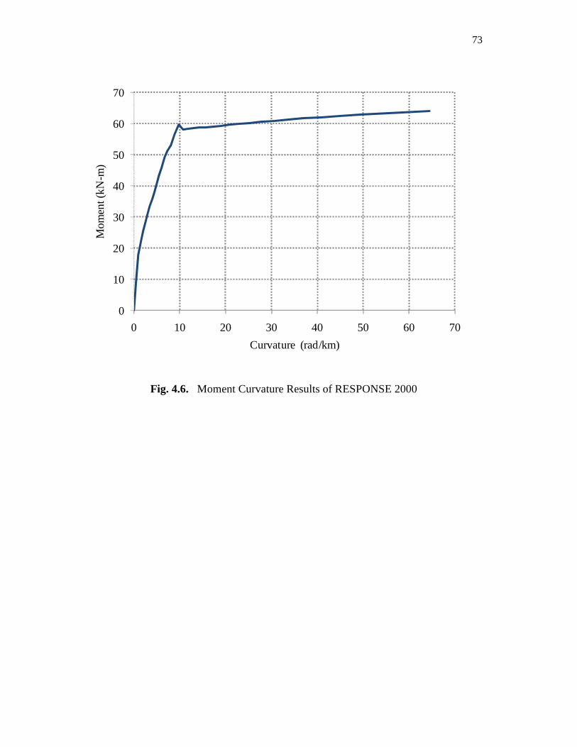
73

Fig. 4.6. Moment Curvature Results of RESPONSE 2000

0

10

20

30

40

50

60

70

0 10 20 30 40 50 60 70

Mom

ent (

kN-m

)

Curvature (rad/km)

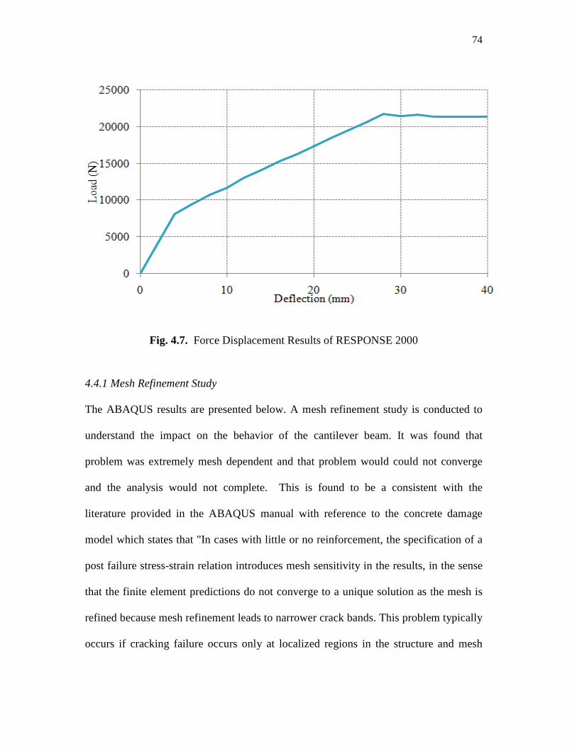
Fig. 4.7. Force Displacement Results of RESPONSE 2000

4.4.1 Mesh Refinement Study

The ABAQUS results are presented below. A mesh refinement study is conducted to

understand the impact on the

problem was extremely mesh dependent and that problem would could not converge

and the analysis would not complete. This is found to be a consistent with the

literature provided in the ABAQUS manual with reference to the concrete damage

model which states that "In cases with little or no reinforcement, the specification of a

post failure stress-strain relation introduces mesh sensitivity in the results, in the sense

that the finite element predictions do not converge to a unique solution

refined because mesh refinement leads to narrower crack bands. This problem typically

occurs if cracking failure occurs only at localized regions in the structure and mesh

Force Displacement Results of RESPONSE 2000

Study


impact on the behavior of the cantilever beam. It was found that




In cases with little or no reinforcement, the specification of a

strain relation introduces mesh sensitivity in the results, in the sense

that the finite element predictions do not converge to a unique solution as the mesh is



74


It was found that




In cases with little or no reinforcement, the specification of a

strain relation introduces mesh sensitivity in the results, in the sense

as the mesh is



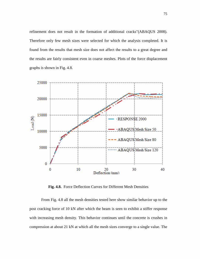
refinement does not result in the formation of additional cracks"

Therefore only few mesh sizes were selected for which the analysis completed. It is

found from the results that mesh size does not affect the results to a great degree and

the results are fairly consistent even in

graphs is shown in Fig. 4.8.

Fig. 4.8. Force Deflection Curves for Different Mesh Densities

From Fig. 4.8 all the mesh densities tested here show similar behavior up to the

post cracking force of 10 kN after which the beam is seen to

with increasing mesh density. This behavior continues until the concrete is

compression at about 21 kN at which all the mesh sizes converge to a single value. The

refinement does not result in the formation of additional cracks"(ABAQUS 2008).



the results are fairly consistent even in coarse meshes. Plots of the force displacement

Force Deflection Curves for Different Mesh Densities

all the mesh densities tested here show similar behavior up to the

rce of 10 kN after which the beam is seen to exhibit a stiffer response

increasing mesh density. This behavior continues until the concrete is

t about 21 kN at which all the mesh sizes converge to a single value. The

75

QUS 2008).



ce displacement

all the mesh densities tested here show similar behavior up to the

exhibit a stiffer response

increasing mesh density. This behavior continues until the concrete is crushes in

t about 21 kN at which all the mesh sizes converge to a single value. The

76

conclusion reached was that the mesh size does not affect the behavior the beam to a

great extent as it was expected. However the problem of convergence faced during the

further mesh refinements proved that the program is able to analyze the problem only

at particular mesh sizes. The determination of a more refined mesh would be

computational intensive as there are a greater number of combinations of elements that

can be produced as the size of the elements reduce. A decision was therefore made to

refine further models until a suitable convergence between the model behavior and the

experimental results was found.

4.4.2 Dilation Angle

The dilation angle can be defined as arctangent of the slope to the yield surface. Based

on the peak values of the compressive and tensile stresses of concrete used here the

value of the dilation angle is determined to be in between 30° to 40°. The model is

now analyzed with these values. A plot comparing the various dilation angles and the

RESPONSE 2000 results are shown in Fig. 4.9. Since the results were very close for all

the dilation angle values, the dilation angle was calculated using the arctangent of yield

surface produced to the Mohr's circles drawn for the peak tension and compressive

stress of concrete. The dilation angle by this method was determined as 40°.

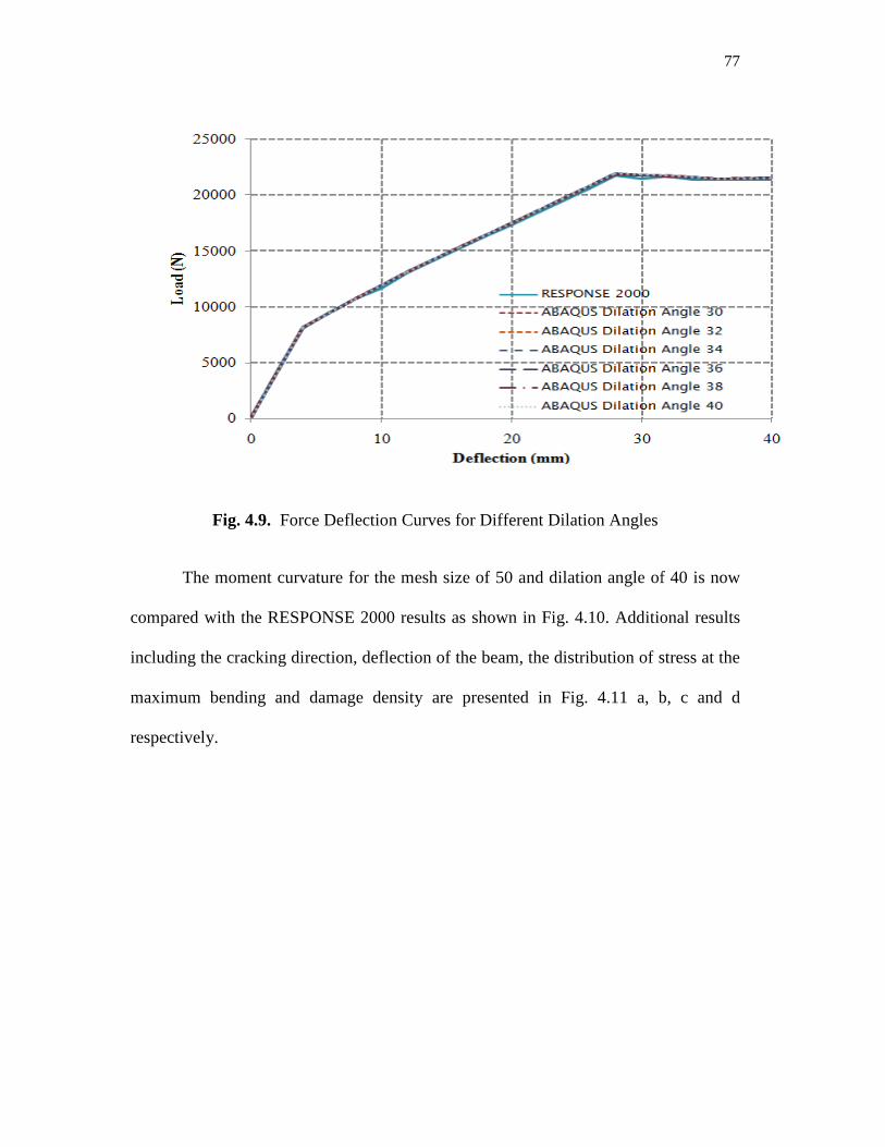
Fig. 4.9. Force Deflection Curves for Different Dilation Angles

The moment curvature for the mesh size of 50 and dilation angle of 40 is now

compared with the RESPONSE 2000 resul

including the cracking direction, deflection of the beam, the distribution of stress at the

maximum bending and damage density

respectively.

Force Deflection Curves for Different Dilation Angles


compared with the RESPONSE 2000 results as shown in Fig. 4.10. Additional

the cracking direction, deflection of the beam, the distribution of stress at the

maximum bending and damage density are presented in Fig. 4.11 a, b, c and d

77


Additional results

the cracking direction, deflection of the beam, the distribution of stress at the

4.11 a, b, c and d

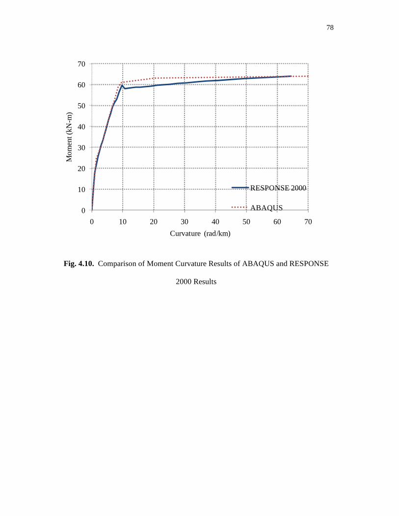
78

Fig. 4.10. Comparison of Moment Curvature Results of ABAQUS and RESPONSE

2000 Results

0

10

20

30

40

50

60

70

0 10 20 30 40 50 60 70

Mom

ent (

kN-m

)

Curvature (rad/km)

RESPONSE 2000

ABAQUS

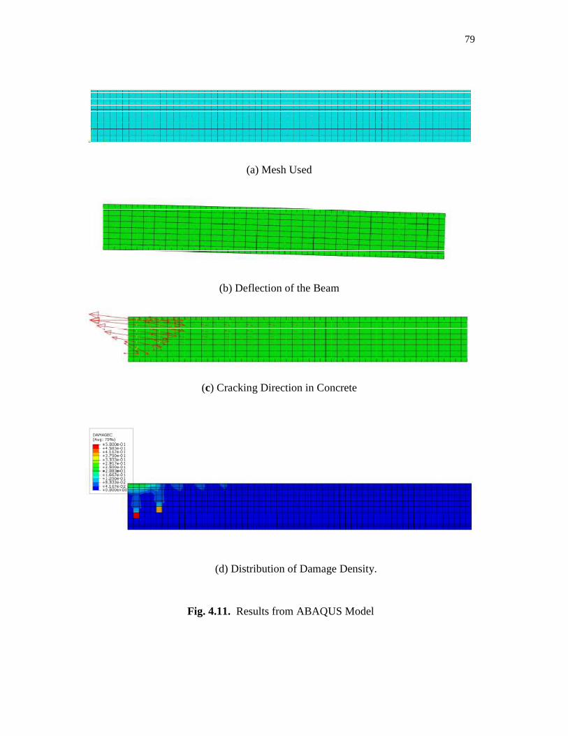
79

(a) Mesh Used

(b) Deflection of the Beam

(c) Cracking Direction in Concrete

(d) Distribution of Damage Density.

Fig. 4.11. Results from ABAQUS Model

80

5. MODELING OF 1.5 ASPECT RATIO COUPLING BEAM

5.1 Introduction

An extensive series of experiments on reinforced concrete coupling beams was

conducted by Galano and Vignoli (2000). The work details the experiments conducted

on a series of 15 coupling beams with varying reinforcement types and different load

cycles. The loading apparatus is also unique to this set of coupling beams. The tests

were conducted on four conventionally reinforced coupling beams, seven diagonally

reinforced coupling beams and four coupling beams provided with rhombic

reinforcement. The aspect ratio for all the beams were kept constant at 1.5. Specimen

P02 was chosen to be modeled for this study. This section details the geometric and

reinforcement detailing of the coupling beam used in the experiment, the finite element

modeling procedures and the comparison between the experimental and the

computational results.

5.2 Description of the Coupling Beam

Specimen P02 was a conventionally reinforced coupling beam with an aspect ratio of

1.5. The beam was 600 mm long with a depth of 400 mm. The adjacent shear walls

were 1100 mm each and 930 mm high. The coupled shear wall system was 150 mm

thick. The beam was reinforced with four 10M (#3 by U.S. designation) bars at top and

bottom and two 6 mm diameter bars were provided as skin reinforcement at mid

height. The reinforcement was extended well into the wall for proper anchoring. The

dimensions of the coupling beam are shown in Fig. 5.1. The reinforcement details are

as shown Fig. 5.2. The main reinforcement ratio ρl is 0.524% and the shear

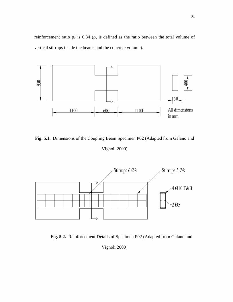
81

reinforcement ratio ρv is 0.84 (ρv is defined as the ratio between the total volume of

vertical stirrups inside the beams and the concrete volume).

Fig. 5.1. Dimensions of the Coupling Beam Specimen P02 (Adapted from Galano and

Vignoli 2000)

Fig. 5.2. Reinforcement Details of Specimen P02 (Adapted from Galano and

Vignoli 2000)

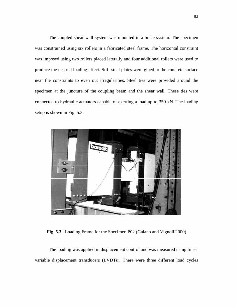
82

The coupled shear wall system was mounted in a brace system. The specimen

was constrained using six rollers in a fabricated steel frame. The horizontal constraint

was imposed using two rollers placed laterally and four additional rollers were used to

produce the desired loading effect. Stiff steel plates were glued to the concrete surface

near the constraints to even out irregularities. Steel ties were provided around the

specimen at the juncture of the coupling beam and the shear wall. These ties were

connected to hydraulic actuators capable of exerting a load up to 350 kN. The loading

setup is shown in Fig. 5.3.

Fig. 5.3. Loading Frame for the Specimen P02 (Galano and Vignoli 2000)

The loading was applied in displacement control and was measured using linear

variable displacement transducers (LVDTs). There were three different load cycles

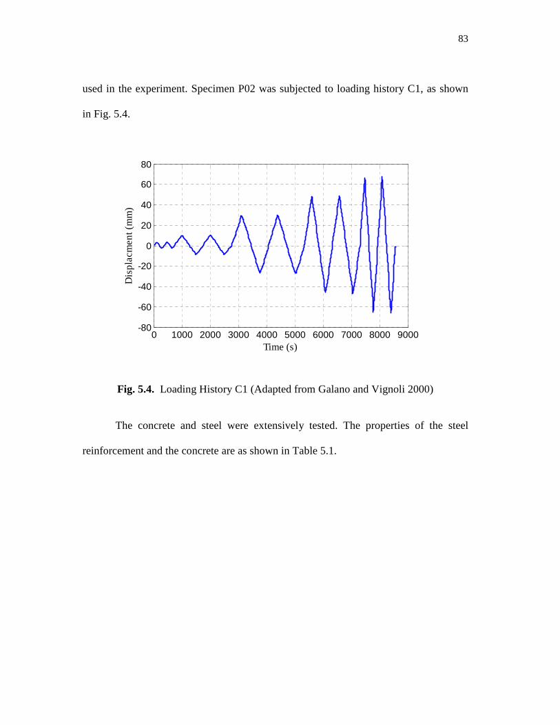
83

used in the experiment. Specimen P02 was subjected to loading history C1, as shown

in Fig. 5.4.

Fig. 5.4. Loading History C1 (Adapted from Galano and Vignoli 2000)

The concrete and steel were extensively tested. The properties of the steel

reinforcement and the concrete are as shown in Table 5.1.

0 1000 2000 3000 4000 5000 6000 7000 8000 9000-80

-60

-40

-20

0

20

40

60

80

Time (s)

Dis

pla

cme

nt (

mm

)

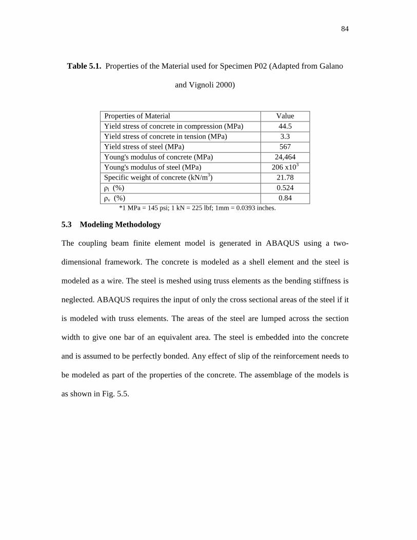
84

Table 5.1. Properties of the Material used for Specimen P02 (Adapted from Galano

and Vignoli 2000)

Properties of Material Value Yield stress of concrete in compression (MPa) 44.5 Yield stress of concrete in tension (MPa) 3.3 Yield stress of steel (MPa) 567 Young's modulus of concrete (MPa) 24,464 Young's modulus of steel (MPa) 206 x103 Specific weight of concrete (kN/m3) 21.78 ρl (%) 0.524 ρv (%) 0.84

*1 MPa = 145 psi; 1 kN = 225 lbf; 1mm = 0.0393 inches.

5.3 Modeling Methodology

The coupling beam finite element model is generated in ABAQUS using a two-

dimensional framework. The concrete is modeled as a shell element and the steel is

modeled as a wire. The steel is meshed using truss elements as the bending stiffness is

neglected. ABAQUS requires the input of only the cross sectional areas of the steel if it

is modeled with truss elements. The areas of the steel are lumped across the section

width to give one bar of an equivalent area. The steel is embedded into the concrete

and is assumed to be perfectly bonded. Any effect of slip of the reinforcement needs to

be modeled as part of the properties of the concrete. The assemblage of the models is

as shown in Fig. 5.5.

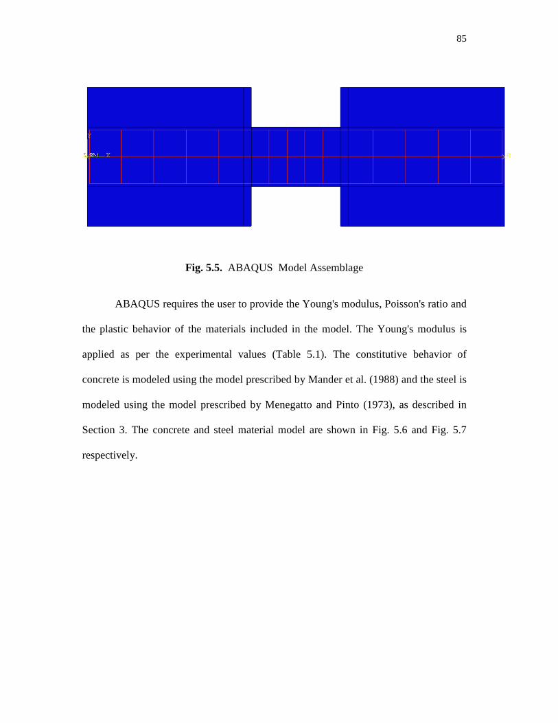
85

Fig. 5.5. ABAQUS Model Assemblage

ABAQUS requires the user to provide the Young's modulus, Poisson's ratio and

the plastic behavior of the materials included in the model. The Young's modulus is

applied as per the experimental values (Table 5.1). The constitutive behavior of

concrete is modeled using the model prescribed by Mander et al. (1988) and the steel is

modeled using the model prescribed by Menegatto and Pinto (1973), as described in

Section 3. The concrete and steel material model are shown in Fig. 5.6 and Fig. 5.7

respectively.

86

Fig. 5.6. Stress-Strain Behavior of Concrete in Compression

0 0.001 0.002 0.003 0.004 0.005 0.006 0.007 0.0080

10

20

30

40

50

Strain

Str

ess

(M

Pa

)

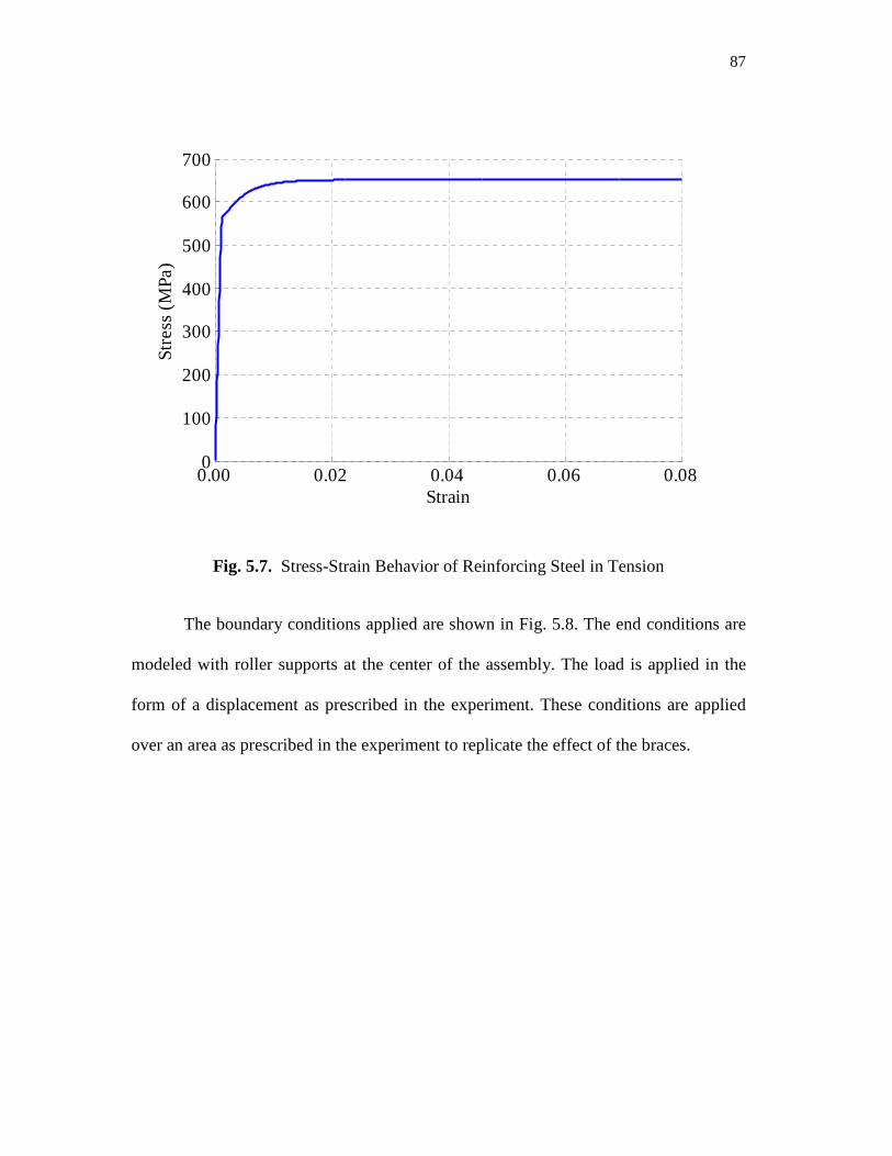
87

Fig. 5.7. Stress-Strain Behavior of Reinforcing Steel in Tension

The boundary conditions applied are shown in Fig. 5.8. The end conditions are

modeled with roller supports at the center of the assembly. The load is applied in the

form of a displacement as prescribed in the experiment. These conditions are applied

over an area as prescribed in the experiment to replicate the effect of the braces.

0.00 0.02 0.04 0.06 0.08 0

100

200

300

400

500

600

700

Strain

Str

ess

(M

Pa

)

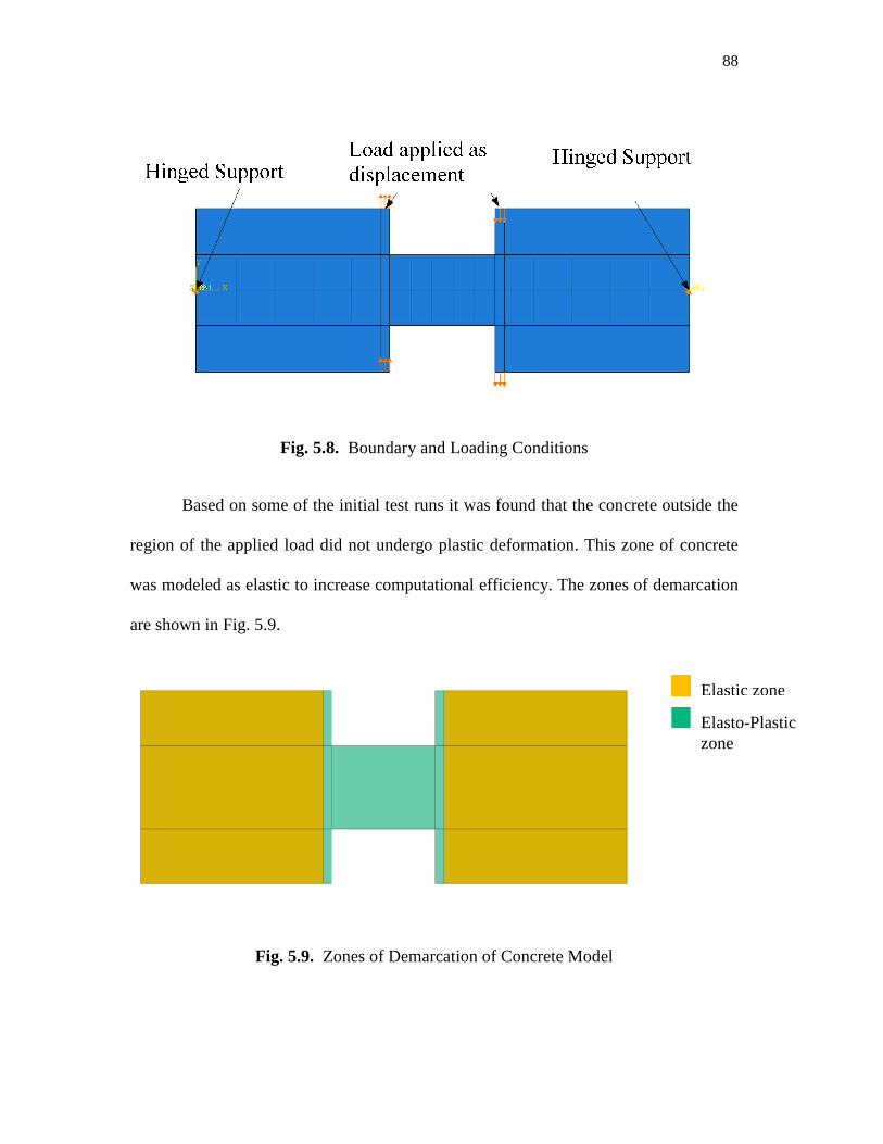
Fig. 5.8

Based on some of the initial test run

region of the applied load did not undergo plastic deformation. This zone of concrete

was modeled as elastic to increase computational efficiency. The zones of dema

are shown in Fig. 5.9.

Fig. 5.9. Zones of Demarcation of Concrete Model

8. Boundary and Loading Conditions

Based on some of the initial test runs it was found that the concrete outside the


was modeled as elastic to increase computational efficiency. The zones of dema

Zones of Demarcation of Concrete Model

88

it was found that the concrete outside the


was modeled as elastic to increase computational efficiency. The zones of demarcation

Elasto-Plastic zone

Elastic zone

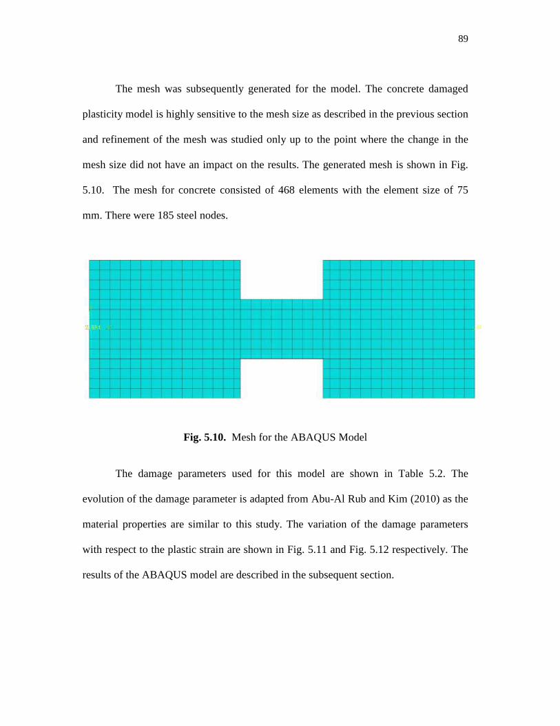
89

The mesh was subsequently generated for the model. The concrete damaged

plasticity model is highly sensitive to the mesh size as described in the previous section

and refinement of the mesh was studied only up to the point where the change in the

mesh size did not have an impact on the results. The generated mesh is shown in Fig.

5.10. The mesh for concrete consisted of 468 elements with the element size of 75

mm. There were 185 steel nodes.

Fig. 5.10. Mesh for the ABAQUS Model

The damage parameters used for this model are shown in Table 5.2. The

evolution of the damage parameter is adapted from Abu-Al Rub and Kim (2010) as the

material properties are similar to this study. The variation of the damage parameters

with respect to the plastic strain are shown in Fig. 5.11 and Fig. 5.12 respectively. The

results of the ABAQUS model are described in the subsequent section.

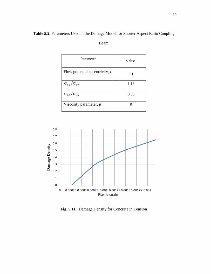
90

Table 5.2. Parameters Used in the Damage Model for Shorter Aspect Ratio Coupling

Beam

Parameter Value

Flow potential eccentricity, ϵ 0.1

b c0 0σ σ 1.16

b c0 0σ σ 0.66

Viscosity parameter, μ 0

Fig. 5.11. Damage Density for Concrete in Tension

0

0.1

0.2

0.3

0.4

0.5

0.6

0.7

0.8

0 0.00025 0.0005 0.00075 0.001 0.00125 0.0015 0.00175 0.002

Dam

age

Den

sity

Plastic strain

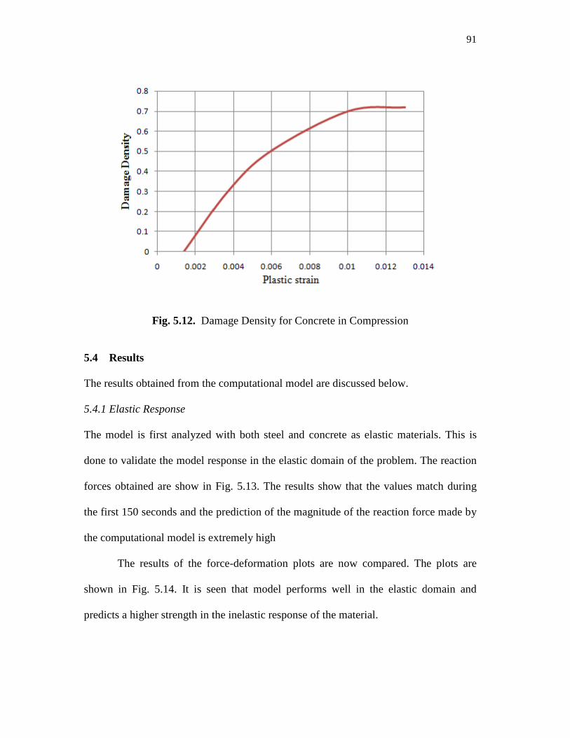
Fig. 5.12. Damage Density for Concrete in Compression

5.4 Results

The results obtained from the computational model are discussed below.

5.4.1 Elastic Response

The model is first analyzed with both steel and concrete as elastic materials. This is

done to validate the model response in the elastic domain of the problem. The reaction

forces obtained are show in

the first 150 seconds and the prediction of the

the computational model is extremely high

The results of the force

shown in Fig. 5.14. It is seen that model performs well in the elastic domain and

predicts a higher strength in the inelastic response of the material.

Damage Density for Concrete in Compression

from the computational model are discussed below.



ned are show in Fig. 5.13. The results show that the values match during

the first 150 seconds and the prediction of the magnitude of the reaction force made by

the computational model is extremely high

The results of the force-deformation plots are now compared. The plots are

5.14. It is seen that model performs well in the elastic domain and

predicts a higher strength in the inelastic response of the material.

91



5.13. The results show that the values match during

reaction force made by

compared. The plots are

5.14. It is seen that model performs well in the elastic domain and

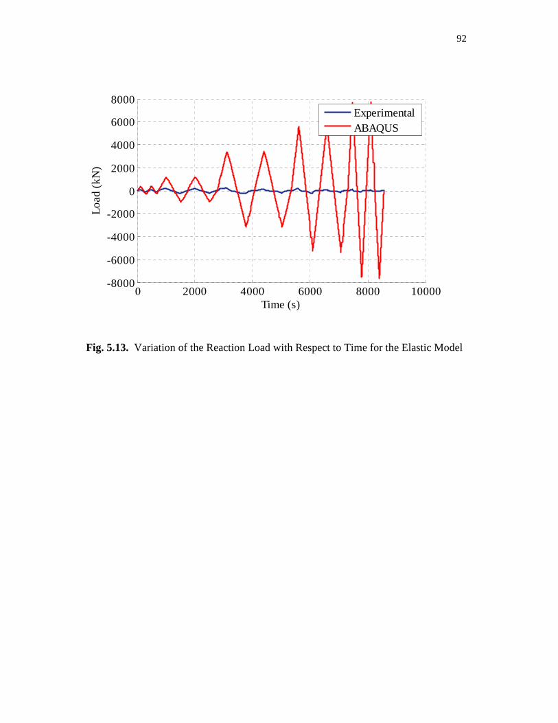
92

Fig. 5.13. Variation of the Reaction Load with Respect to Time for the Elastic Model

0 2000 4000 6000 8000 10000-8000

-6000

-4000

-2000

0

2000

4000

6000

8000

Time (s)

Loa

d (

kN)

Experimental ABAQUS

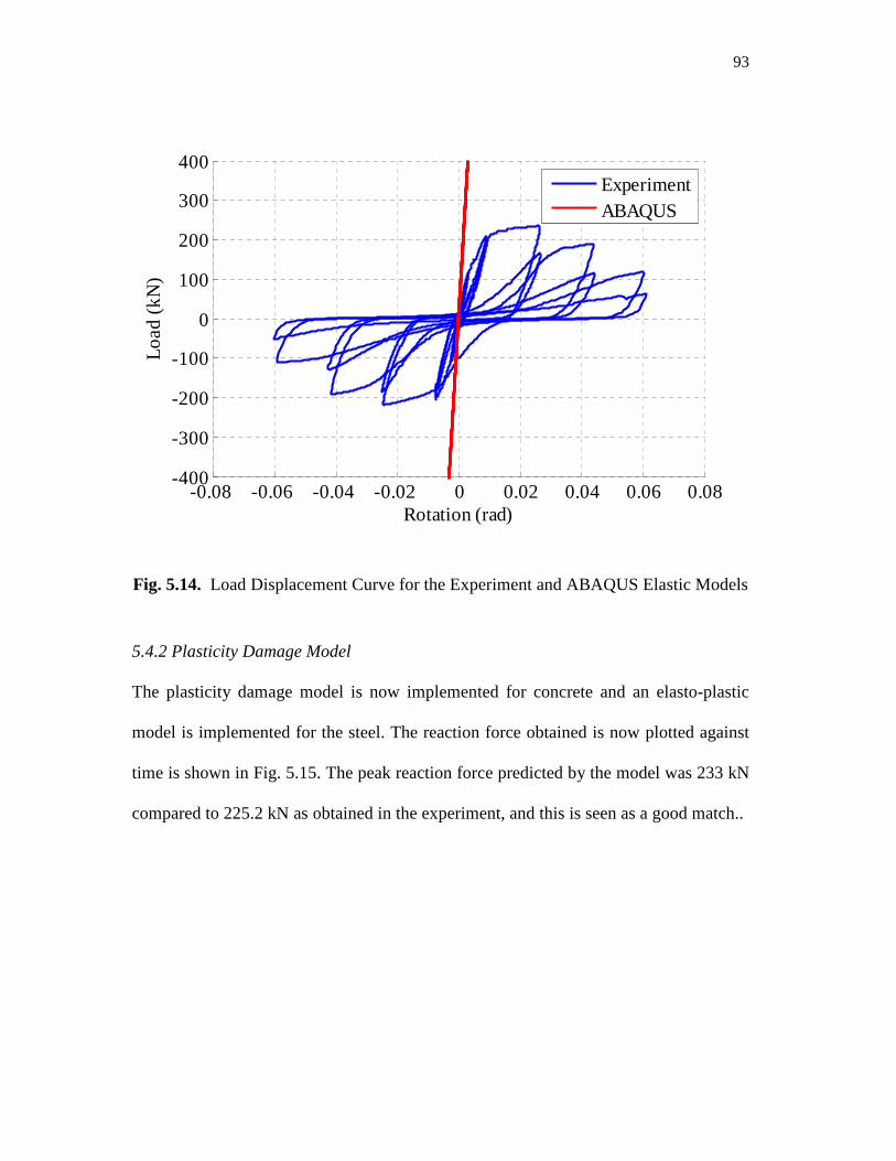
93

Fig. 5.14. Load Displacement Curve for the Experiment and ABAQUS Elastic Models

5.4.2 Plasticity Damage Model

The plasticity damage model is now implemented for concrete and an elasto-plastic

model is implemented for the steel. The reaction force obtained is now plotted against

time is shown in Fig. 5.15. The peak reaction force predicted by the model was 233 kN

compared to 225.2 kN as obtained in the experiment, and this is seen as a good match..

-0.08 -0.06 -0.04 -0.02 0 0.02 0.04 0.06 0.08-400

-300

-200

-100

0

100

200

300

400

Rotation (rad)

Loa

d (

kN)

ExperimentABAQUS

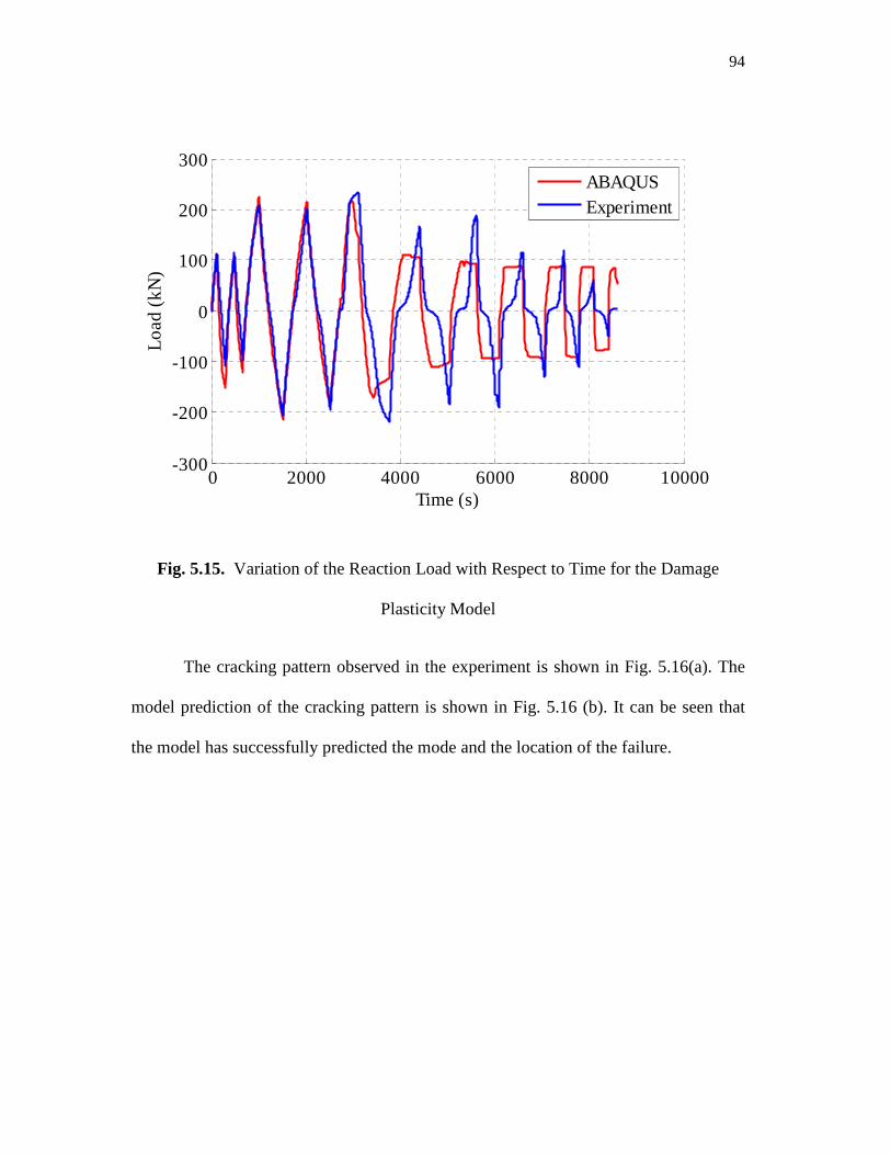
94

Fig. 5.15. Variation of the Reaction Load with Respect to Time for the Damage

Plasticity Model

The cracking pattern observed in the experiment is shown in Fig. 5.16(a). The

model prediction of the cracking pattern is shown in Fig. 5.16 (b). It can be seen that

the model has successfully predicted the mode and the location of the failure.

0 2000 4000 6000 8000 10000-300

-200

-100

0

100

200

300

Time (s)

Loa

d (

kN)

ABAQUSExperiment

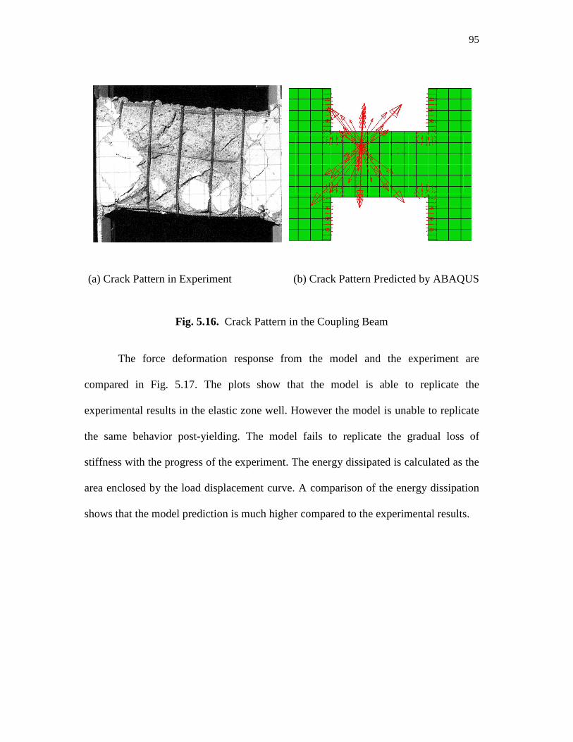
95

(a) Crack Pattern in Experiment (b) Crack Pattern Predicted by ABAQUS

Fig. 5.16. Crack Pattern in the Coupling Beam

The force deformation response from the model and the experiment are

compared in Fig. 5.17. The plots show that the model is able to replicate the

experimental results in the elastic zone well. However the model is unable to replicate

the same behavior post-yielding. The model fails to replicate the gradual loss of

stiffness with the progress of the experiment. The energy dissipated is calculated as the

area enclosed by the load displacement curve. A comparison of the energy dissipation

shows that the model prediction is much higher compared to the experimental results.

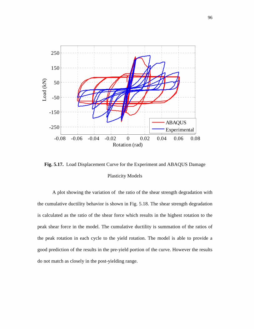
96

Fig. 5.17. Load Displacement Curve for the Experiment and ABAQUS Damage

Plasticity Models

A plot showing the variation of the ratio of the shear strength degradation with

the cumulative ductility behavior is shown in Fig. 5.18. The shear strength degradation

is calculated as the ratio of the shear force which results in the highest rotation to the

peak shear force in the model. The cumulative ductility is summation of the ratios of

the peak rotation in each cycle to the yield rotation. The model is able to provide a

good prediction of the results in the pre-yield portion of the curve. However the results

do not match as closely in the post-yielding range.

-0.08 -0.06 -0.04 -0.02 0 0.02 0.04 0.06 0.08

-250

-150

-50

50

150

250

Rotation (rad)

Loa

d (

kN)

ABAQUSExperimental

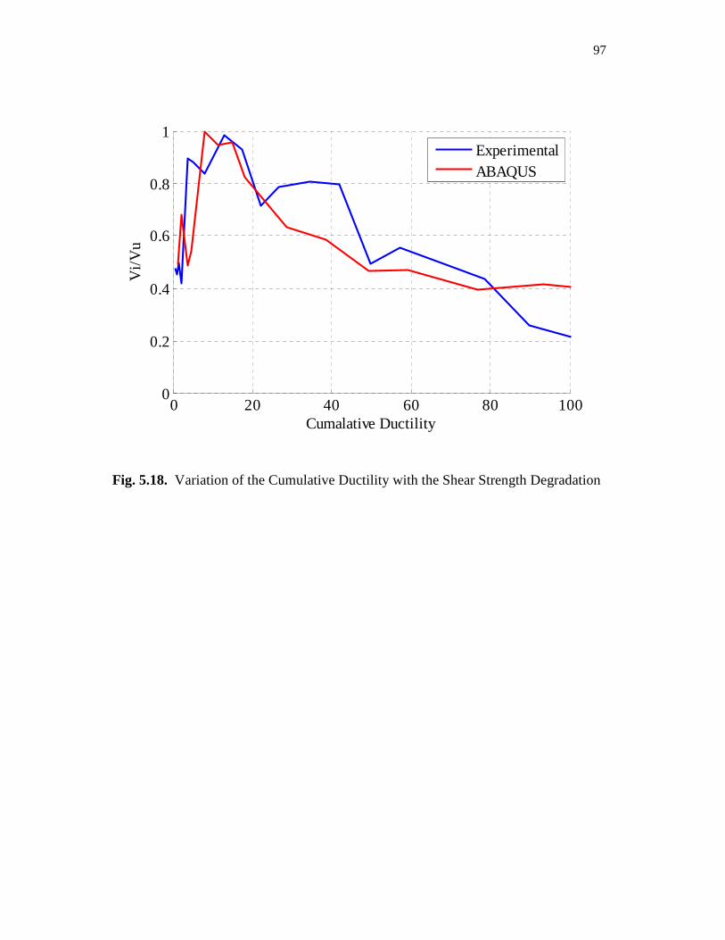
97

Fig. 5.18. Variation of the Cumulative Ductility with the Shear Strength Degradation

0 20 40 60 80 1000

0.2

0.4

0.6

0.8

1

Cumalative Ductility

Vi/V

u

ExperimentalABAQUS

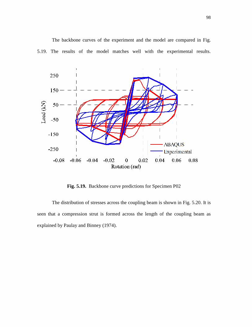
The backbone curves of the experiment and the model are compared

5.19. The results of the model

Fig. 5.19. Backbone curve predictions for Specimen P02

The distribution of stresses across the coupling beam is shown in Fig. 5.20. It is

seen that a compression strut is formed across the length of the coupling beam as

explained by Paulay and Binney (1974).

The backbone curves of the experiment and the model are compared

. The results of the model matches well with the experimental result

Backbone curve predictions for Specimen P02




98

The backbone curves of the experiment and the model are compared in Fig.

well with the experimental results.



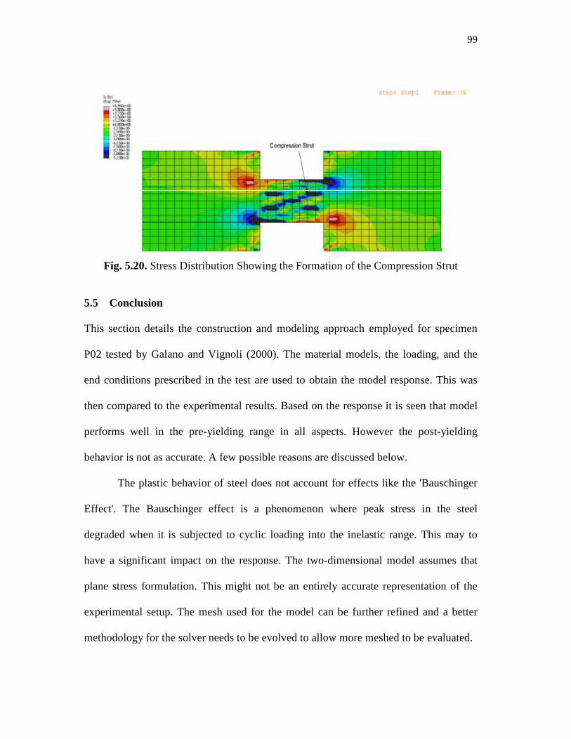
99

Fig. 5.20. Stress Distribution Showing the Formation of the Compression Strut

5.5 Conclusion

This section details the construction and modeling approach employed for specimen

P02 tested by Galano and Vignoli (2000). The material models, the loading, and the

end conditions prescribed in the test are used to obtain the model response. This was

then compared to the experimental results. Based on the response it is seen that model

performs well in the pre-yielding range in all aspects. However the post-yielding

behavior is not as accurate. A few possible reasons are discussed below.

The plastic behavior of steel does not account for effects like the 'Bauschinger

Effect'. The Bauschinger effect is a phenomenon where peak stress in the steel

degraded when it is subjected to cyclic loading into the inelastic range. This may to

have a significant impact on the response. The two-dimensional model assumes that

plane stress formulation. This might not be an entirely accurate representation of the

experimental setup. The mesh used for the model can be further refined and a better

methodology for the solver needs to be evolved to allow more meshed to be evaluated.

100

6. MODELING OF THE 3.6 ASPECT RATIO BEAM

6.1 Introduction

The following section describes the simulation of the experimental work conducted by

Bristowe (2000). The experiments were aimed at developing constitutive relations for

predicting the behavior of normal and high strength concrete specimens subjected to

cyclic loading. As part of the study four coupling beams were tested using normal and

high strength concrete with different reinforcement ratio. The aspect ratio was

maintained at 3.6 so to compare their behaviors. This experiment utilized the test setup

developed by Harries (1995). This section details the test setup used by Bristowe, the

modeling methodology, and the comparison of the results.

6.2 Description of the Coupling Beam

The experiments Bristowe (2000) included details four conventionally reinforced

concrete coupling beams constructed with normal and high strength concrete

designated as NR2, NR4, MR2, MR4. The specimen were labeled using NR to denote

for normally reinforced concrete and MR for high strength concrete. The coupling

beams were 500 mm deep and 1800 mm long and 300 mm thick with an aspect ratio of

3.6. The beams were reinforced with three 25M (#8 by U.S. designation) bars at top

bars at top and bottom and two 10M (#3 by U.S. designation) bars acting as skin

reinforcement. The longitudinal bars were embedded to a length of 1100 mm into the

wall. The shear wall was 300 mm thick, 1500 mm long, and 1500 mm high. A region

of concentrated reinforcement consisting of four 25M vertical reinforcing bars was

provided adjoining to the beams in the walls. The concentrated reinforcement was

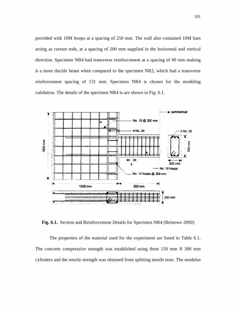
101

provided with 10M hoops at a spacing of 250 mm. The wall also contained 10M bars

acting as curtain rods, at a spacing of 200 mm supplied in the horizontal and vertical

direction. Specimen NR4 had transverse reinforcement at a spacing of 90 mm making

it a more ductile beam when compared to the specimen NR2, which had a transverse

reinforcement spacing of 131 mm. Specimen NR4 is chosen for the modeling

validation. The details of the specimen NR4 is are shown in Fig. 6.1.

Fig. 6.1. Section and Reinforcement Details for Specimen NR4 (Bristowe 2000)

The properties of the material used for the experiment are listed in Table 6.1.

The concrete compressive strength was established using three 150 mm X 300 mm

cylinders and the tensile strength was obtained from splitting tensile tests. The modulus

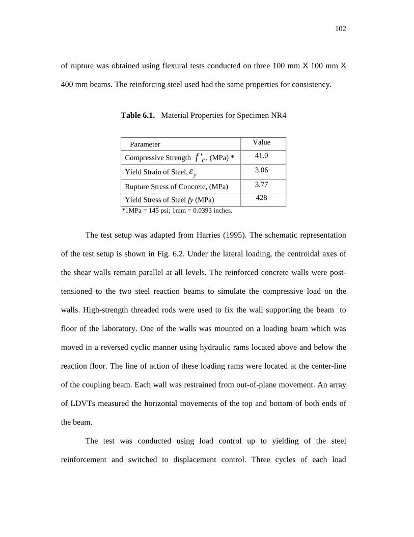
102

of rupture was obtained using flexural tests conducted on three 100 mm X 100 mm X

400 mm beams. The reinforcing steel used had the same properties for consistency.

Table 6.1. Material Properties for Specimen NR4

Parameter Value

Compressive Strength cf ' , (MPa) * 41.0

Yield Strain of Steel, yε 3.06

Rupture Stress of Concrete, (MPa) 3.77

Yield Stress of Steel fy (MPa) 428

*1MPa = 145 psi; 1mm = 0.0393 inches.

The test setup was adapted from Harries (1995). The schematic representation

of the test setup is shown in Fig. 6.2. Under the lateral loading, the centroidal axes of

the shear walls remain parallel at all levels. The reinforced concrete walls were post-

tensioned to the two steel reaction beams to simulate the compressive load on the

walls. High-strength threaded rods were used to fix the wall supporting the beam to

floor of the laboratory. One of the walls was mounted on a loading beam which was

moved in a reversed cyclic manner using hydraulic rams located above and below the

reaction floor. The line of action of these loading rams were located at the center-line

of the coupling beam. Each wall was restrained from out-of-plane movement. An array

of LDVTs measured the horizontal movements of the top and bottom of both ends of

the beam.

The test was conducted using load control up to yielding of the steel

reinforcement and switched to displacement control. Three cycles of each load

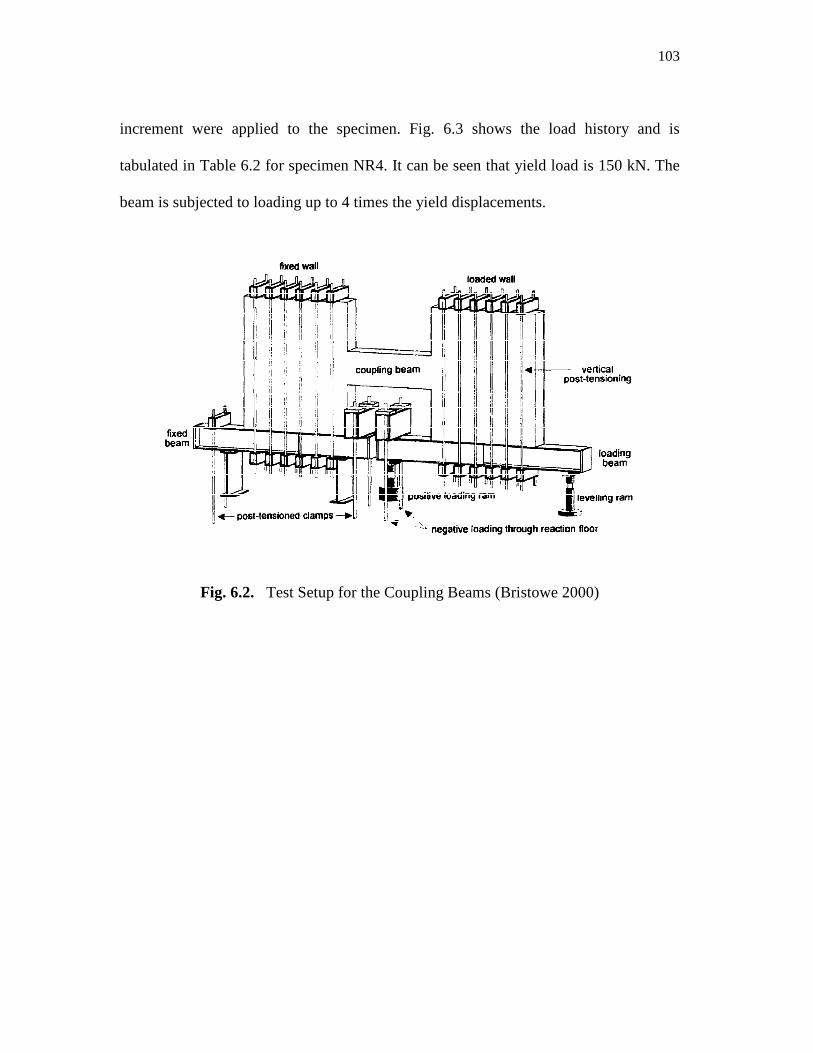
103

increment were applied to the specimen. Fig. 6.3 shows the load history and is

tabulated in Table 6.2 for specimen NR4. It can be seen that yield load is 150 kN. The

beam is subjected to loading up to 4 times the yield displacements.

Fig. 6.2. Test Setup for the Coupling Beams (Bristowe 2000)

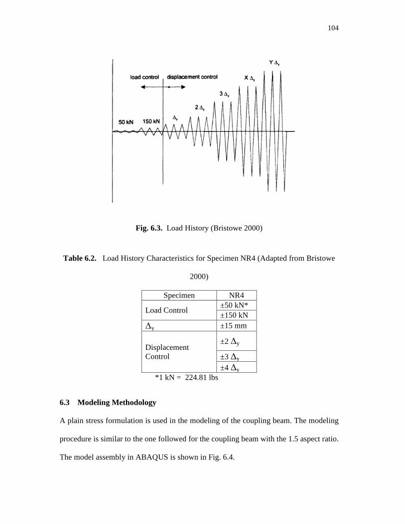
104

Fig. 6.3. Load History (Bristowe 2000)

Table 6.2. Load History Characteristics for Specimen NR4 (Adapted from Bristowe

2000)

Specimen NR4

Load Control ±50 kN* ±150 kN

∆y ±15 mm

Displacement Control

±2 ∆y

±3 ∆y ±4 ∆y

*1 kN = 224.81 lbs

6.3 Modeling Methodology

A plain stress formulation is used in the modeling of the coupling beam. The modeling

procedure is similar to the one followed for the coupling beam with the 1.5 aspect ratio.

The model assembly in ABAQUS is shown in Fig. 6.4.

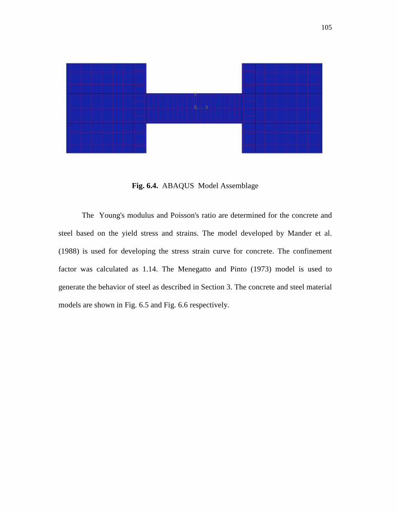
105

Fig. 6.4. ABAQUS Model Assemblage

The Young's modulus and Poisson's ratio are determined for the concrete and

steel based on the yield stress and strains. The model developed by Mander et al.

(1988) is used for developing the stress strain curve for concrete. The confinement

factor was calculated as 1.14. The Menegatto and Pinto (1973) model is used to

generate the behavior of steel as described in Section 3. The concrete and steel material

models are shown in Fig. 6.5 and Fig. 6.6 respectively.

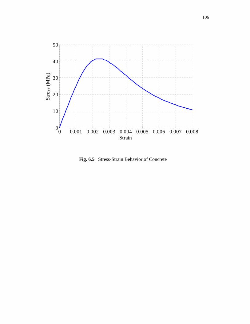
106

Fig. 6.5. Stress-Strain Behavior of Concrete

0 0.001 0.002 0.003 0.004 0.005 0.006 0.007 0.0080

10

20

30

40

50

Strain

Str

ess

(M

Pa

)

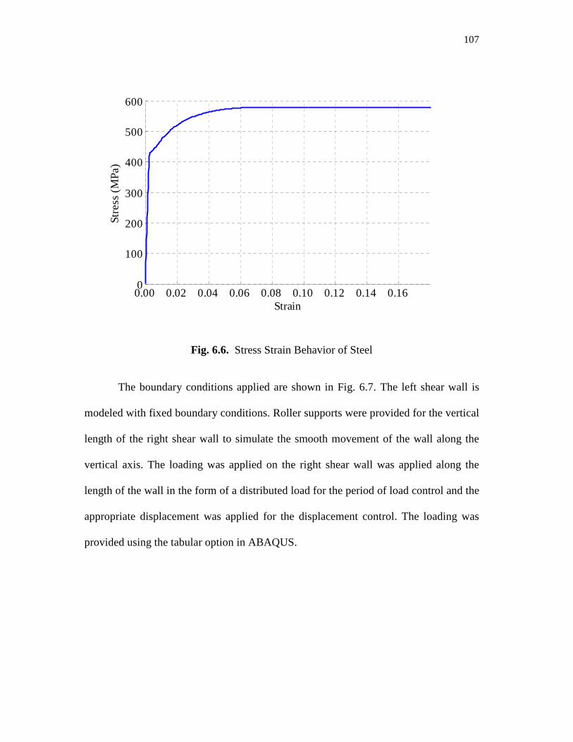
107

Fig. 6.6. Stress Strain Behavior of Steel

The boundary conditions applied are shown in Fig. 6.7. The left shear wall is

modeled with fixed boundary conditions. Roller supports were provided for the vertical

length of the right shear wall to simulate the smooth movement of the wall along the

vertical axis. The loading was applied on the right shear wall was applied along the

length of the wall in the form of a distributed load for the period of load control and the

appropriate displacement was applied for the displacement control. The loading was

provided using the tabular option in ABAQUS.

0.00 0.02 0.04 0.06 0.08 0.10 0.12 0.14 0.16 0

100

200

300

400

500

600

Strain

Str

ess

(M

Pa

)

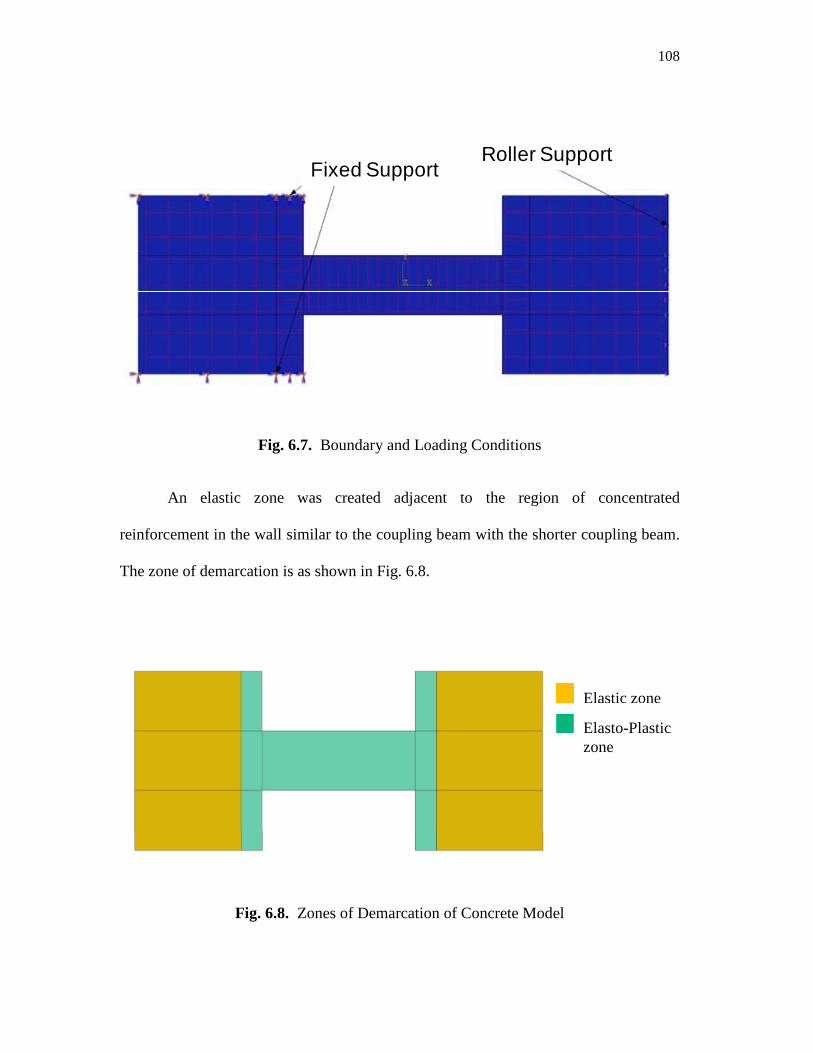
108

Fig. 6.7. Boundary and Loading Conditions

An elastic zone was created adjacent to the region of concentrated

reinforcement in the wall similar to the coupling beam with the shorter coupling beam.

The zone of demarcation is as shown in Fig. 6.8.

Fig. 6.8. Zones of Demarcation of Concrete Model

Fixed SupportRoller Support

Elasto-Plastic zone

Elastic zone

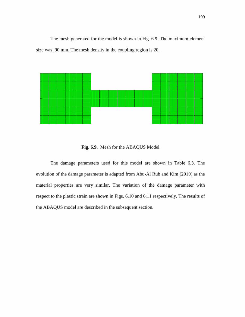
109

The mesh generated for the model is shown in Fig. 6.9. The maximum element

size was 90 mm. The mesh density in the coupling region is 20.

Fig. 6.9. Mesh for the ABAQUS Model

The damage parameters used for this model are shown in Table 6.3. The

evolution of the damage parameter is adapted from Abu-Al Rub and Kim (2010) as the

material properties are very similar. The variation of the damage parameter with

respect to the plastic strain are shown in Figs. 6.10 and 6.11 respectively. The results of

the ABAQUS model are described in the subsequent section.

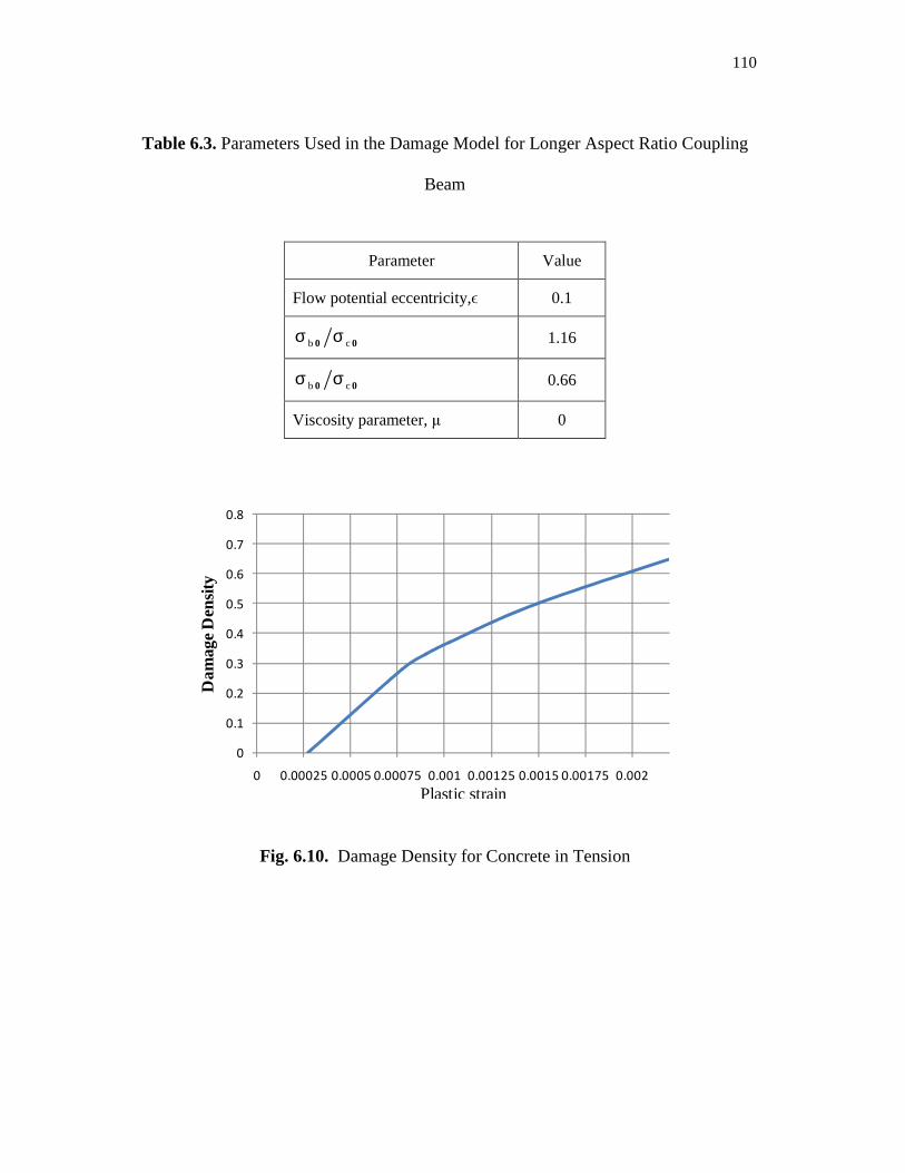
110

Table 6.3. Parameters Used in the Damage Model for Longer Aspect Ratio Coupling

Beam

Parameter Value

Flow potential eccentricity,ϵ 0.1

b c0 0σ σ 1.16

b c0 0σ σ 0.66

Viscosity parameter, µ 0

Fig. 6.10. Damage Density for Concrete in Tension

0

0.1

0.2

0.3

0.4

0.5

0.6

0.7

0.8

0 0.00025 0.0005 0.00075 0.001 0.00125 0.0015 0.00175 0.002

Dam

age

Den

sity

Plastic strain

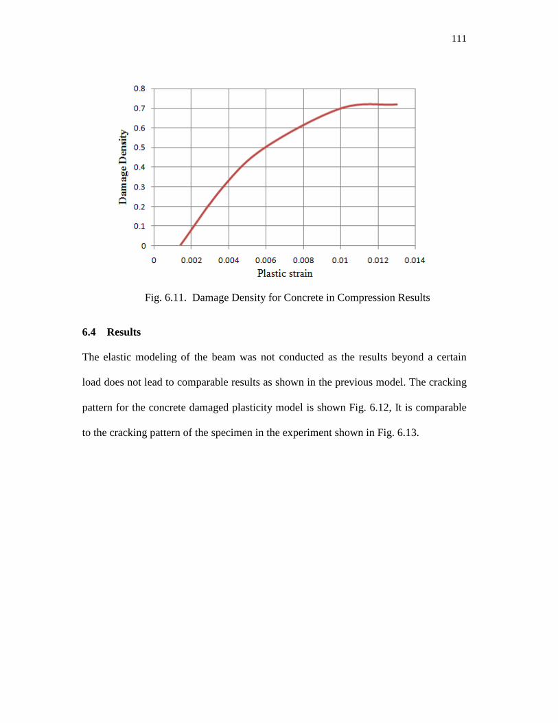
Fig. 6.11. Damage Density for Concrete in Compression

6.4 Results

The elastic modeling of the beam was not conducted as the results beyond a certain

load does not lead to comparable results as shown in the previous model. The crackin

pattern for the concrete damaged

to the cracking pattern of the specimen in the

Damage Density for Concrete in Compression Results


load does not lead to comparable results as shown in the previous model. The crackin

concrete damaged plasticity model is shown Fig. 6.12, It is comparable

cracking pattern of the specimen in the experiment shown in Fig. 6.13.

111

Results


load does not lead to comparable results as shown in the previous model. The cracking

is comparable

13.

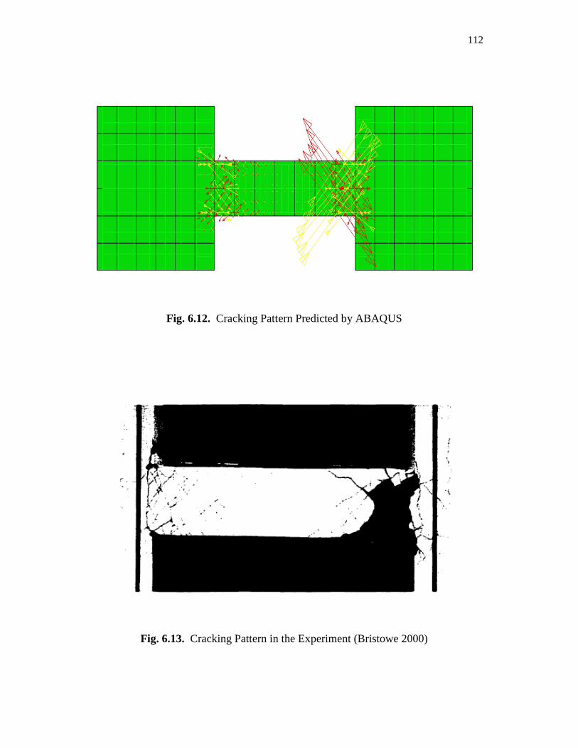
112

Fig. 6.12. Cracking Pattern Predicted by ABAQUS

Fig. 6.13. Cracking Pattern in the Experiment (Bristowe 2000)

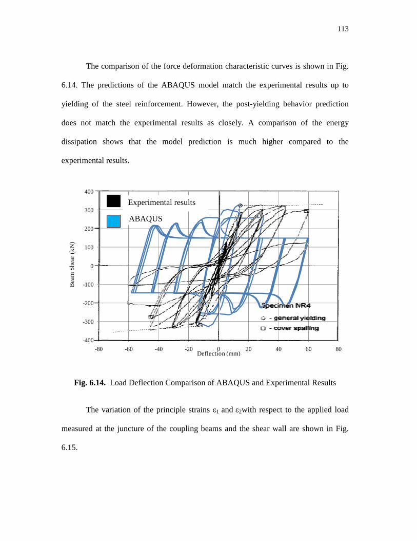
113

The comparison of the force deformation characteristic curves is shown in Fig.

6.14. The predictions of the ABAQUS model match the experimental results up to

yielding of the steel reinforcement. However, the post-yielding behavior prediction

does not match the experimental results as closely. A comparison of the energy

dissipation shows that the model prediction is much higher compared to the

experimental results.

Fig. 6.14. Load Deflection Comparison of ABAQUS and Experimental Results

The variation of the principle strains ε1 and ε2with respect to the applied load

measured at the juncture of the coupling beams and the shear wall are shown in Fig.

6.15.

-400

-300

-200

-100

0

100

200

300

400

-80 -60 -40 -20 0 20 40 60 80

Be

am

Sh

ea

r (k

N)

Deflection (mm)

ABAQUS

Experimental results

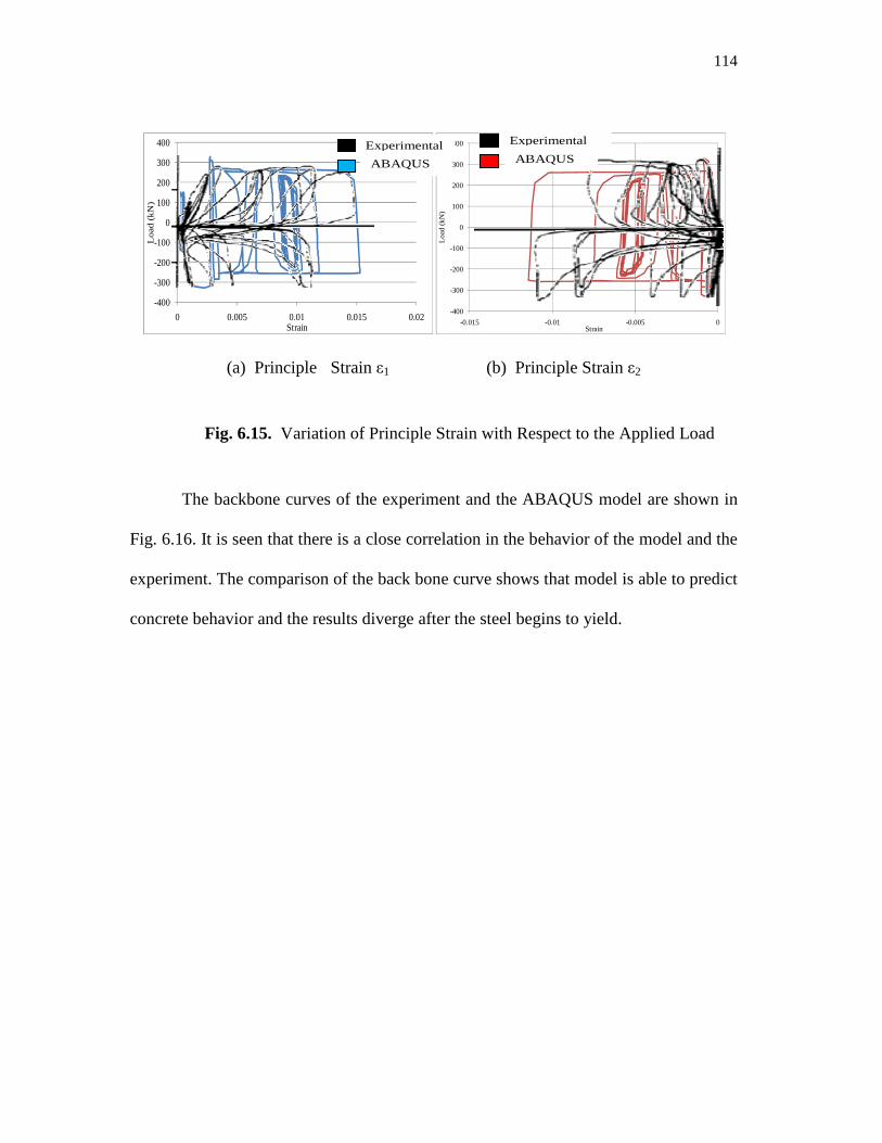
114

(a) Principle Strain ε1 (b) Principle Strain ε2

Fig. 6.15. Variation of Principle Strain with Respect to the Applied Load

The backbone curves of the experiment and the ABAQUS model are shown in

Fig. 6.16. It is seen that there is a close correlation in the behavior of the model and the

experiment. The comparison of the back bone curve shows that model is able to predict

concrete behavior and the results diverge after the steel begins to yield.

-400

-300

-200

-100

0

100

200

300

400

0 0.005 0.01 0.015 0.02

Lo

ad

(kN

)

Strain

-400

-300

-200

-100

0

100

200

300

400

-0.015 -0.01 -0.005 0

Lo

ad

(kN

)

Strain

ABAQUS

Experimental

ABAQUS

Experimental

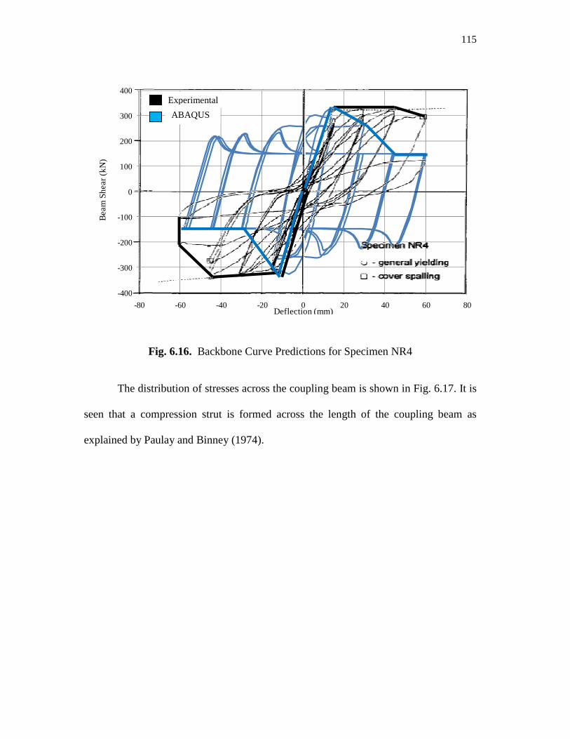
115

Fig. 6.16. Backbone Curve Predictions for Specimen NR4




-400

-300

-200

-100

0

100

200

300

400

-80 -60 -40 -20 0 20 40 60 80

Be

am

Sh

ea

r (k

N)

Deflection (mm)

ABAQUS

Experimental

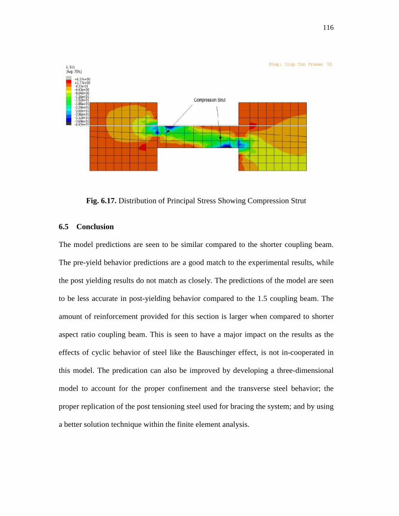
116

Fig. 6.17. Distribution of Principal Stress Showing Compression Strut

6.5 Conclusion

The model predictions are seen to be similar compared to the shorter coupling beam.

The pre-yield behavior predictions are a good match to the experimental results, while

the post yielding results do not match as closely. The predictions of the model are seen

to be less accurate in post-yielding behavior compared to the 1.5 coupling beam. The

amount of reinforcement provided for this section is larger when compared to shorter

aspect ratio coupling beam. This is seen to have a major impact on the results as the

effects of cyclic behavior of steel like the Bauschinger effect, is not in-cooperated in

this model. The predication can also be improved by developing a three-dimensional

model to account for the proper confinement and the transverse steel behavior; the

proper replication of the post tensioning steel used for bracing the system; and by using

a better solution technique within the finite element analysis.

117

7. CONCLUSIONS AND SCOPE FOR FURTHER WORK

7.1 Summary

This research was conducted to develop a computational modeling approach to

simulate the behavior of conventionally reinforced coupling beams subjected to cyclic

loading. The computational model generated here makes use of the concrete damaged

plasticity model available in the commercial finite element modeling package

ABAQUS to simulate the behavior of concrete. A calibration model using a cantilever

beam is first produced to generate some of the key parameters in the model that are

later adapted into modeling of two coupling beams of varying aspect ratios of 1.5 and

3.6. The geometric, material, and loading values are adapted from experimental

specimens reported in the literature, and the experimental results are then used to

validate the computational models. The findings from this study are intended to

provide guidance on finite element modeling of conventionally reinforced concrete

coupling beams under cyclic lateral loading.

7.2 Conclusions

The following conclusions are observed based on the results of this study:

1. The calibration model for the cantilever beam developed in ABAQUS

replicated the results predicted by the analytical program RESPONSE 2000.

The model was found to perform well for monotonic loading into the nonlinear

range, as all the results proved to be a good match.

2. The computational results for the 1.5 aspect ratio coupling beam indicate the

following:

118

o The ABAQUS model predicted the experimental response accurately

under cyclic loading up to the yielding of the steel. However, the

prediction was less accurate into the inelastic range.

o The backbone curve predicted by the ABAQUS model shows a close

correlation with the experimental results into the inelastic range.

3. The prediction of the region of damage within the coupling beam matched the

experimental results.The computational results for the 3.6 aspect ratio coupling

beam were similar to the 1.5 aspect ratio coupling beam.

o The ABAQUS model predicted the experimental response accurately

under cyclic loading up to the yielding of the steel. The prediction is

less accurate post yielding and this difference is greater compared to the

shorter aspect ratio coupling beam. This is due to the higher

reinforcement ratio in the 3.6 aspect ratio coupling beam.

o The backbone curve predicted by the ABAQUS model shows a close

correlation with the experimental results into the inelastic range.

o The prediction of the region of damage within the coupling beam

matched the experimental results.

o The prediction of the energy dissipated was seen to be higher compared

to the experimental values.

4. Differences in the behavior of the two coupling beam specimens were also

observed. The displacements experienced by the coupling beams are of the

same order. However, the 3.6 aspect ratio coupling beam experienced a greater

119

amount of damage compared to the 1.5 aspect ratio coupling beam. This change

in the behavior may be due to the difference in load cycles and the loading and

support conditions employed in the experiments. It is also observed that the

longer coupling beam had a greater density of transverse reinforcement and

subsequently has greater displacement ductility.

7.3 Scope for Further Work

The comparison of the analytical and experimental results indicates that the ABAQUS

model can be further improved. The following recommendations are made for future

work:

1. The steel model used here only incorporates the steel isotropic hardening;

however, its behavior under cyclic load should also be included.

2. The assumptions made on the variation of the damage parameter can be based

on a more refined analytical model. However, there was not sufficient

experimental data to describe the material behavior into the inelastic range for

the selected experiments.

3. Truss elements are used to model the steel in this study. The effect of the

bending stiffness could be included for a more refined model, although its

contribution is not expected to be significant.

4. The steel could be meshed using cylindrical shell elements for more accurate

simulation of the behavior of the steel. The cylindrical shell element, however,

has much higher computational requirements.

120

5. The static solver used for this study is not robust enough because it does not

work for all meshes. A suitable alternative solver needs to be developed to

understand the effects of mesh refinement.

6. A study could be conducted on the influence of confinement of the concrete

core on the modeling behavior. The experiments had reported that the cover

concrete spalls off under high loading, the effects of lower confinement in the

cover region should be included in the model.

7. The time required based on the mesh size is not studied here, this needs to be

included.

8. The effect of parameters like viscosity and rate effects in concrete needs to be

considered.

9. A three-dimensional finite element model needs to be produced to better

understand the accuracy of the finite element procedure.

10. A comparison should be made between two-dimensional and three-dimensional

modeling approaches in terms of results obtained and computational efficiency

of the models.

121

REFERENCES

ABAQUS (2008). ABAQUS Version 6.8-3, Computer Program, ABAQUS, Inc, Providence, Rhode Island.

Abu Al-Rub, R. K., and Kim, S. M. (2010), "Computational applications of a coupled plasticity-damage constitutive model for simulating plain concrete fracture." Proc., Eng Fract Mech, 77(10), 1577-1603.

ACI Committee 318 (2008). " Building code requirements for structural concrete (ACI 318-08) and Commentary (318R-08)." American Concrete Institute, Farmington Hills, Michigan.

Barney, G.B., Shiu, K.N., Rabbat, B.G., Fiorato, A.E., Russell, H.G., and Corley, W.G. (1980)."Behavior of coupling beams under load reversals." Research and Development Bulletin RD068.01B. Portland Cement Association, Skokie, Illinois.

Bentz, E. C. (2000). "Sectional analysis of reinforced concrete members." Ph.D. dissertation, University of Toronto, Canada.

Bristowe, S. (2000). "Seismic response of normal and high strength concrete members." Ph.D. dissertation, McGill University, Canada.

Brower, J. O. (2008). "Analytical investigation into the effect of axial restraint on the stiffness and ductility of diagonally reinforced concrete coupling beams." M.S thesis , University of Cincinnati, Ohio.

Fortney, P. J. (2005). "The next generation of coupling beams." PhD dissertation, University of Cincinnati, Ohio.

Fortney, P., Rassati, G., and Shahrooz, B. (2008). "Investigation on effect of transverse reinforcement on performance of diagonally reinforced coupling beams." ACI Structural Journal, 105(6).

Galano, L., and Vignoli, A. (2000). "Seismic behavior of short coupling beams with different reinforcement layouts." ACI Structural Journal, 97(6), 876-885.

Harries, K. A. (1995). "Seismic design and retrofit of coupled walls using structural steel." Ph.D, McGill University, Canada.

Hindi, R., and Hassan, M. (2007). "Simplified trilinear behavior of diagonally reinforced coupling beams." ACI Structural Journal, 5(2) 199-206.

122

Kwan, A., and Zhao, Z. (2002). "Cyclic behaviour of deep reinforced concrete coupling beams." Proceedings of the Institution of Civil Engineers-Structures and Buildings, 152(3), 283-294.

Mander, J. B., Priestley, M. J. N., and Park, R. (1988). "Theoretical stress-strain model for confined concrete." Journal of Structural Engineering, 114(8), 1804-1826.

Mander, J., and Priestley, M. (1988). "Observed Stress Strain Behavior of Confined Concrete." Journal of Structural Engineering, 114, 1827-1849.

Menegotto, M., and Pinto, P. E. (1973). " Method of analysis for cyclically loaded reinforced concrete plane frames including changes in geometry and non-elastic behavior of elements under combined normal force and bending." IABSE Symposium on the Resistance and Ultimate Deformability of Structures Acted on by Well-defined Repeated Loads, Lisbon Portugal, 15-22.

Paparoni, M. (1972). "Model studies of coupling beams." International Conference on Tall Concrete and Masonry Buildings, Lehigh University, Bethlehem, Pennsylvania, 671-681.

Paulay, T. (1970). "An elasto-plastic analysis of coupled shear walls." Journal of American Concrete Institute,67(11), 915-922.

Paulay, T. (1971). "Coupling beams of reinforced concrete shear walls." Journal of the Structural Division, 97(3), 843-862.

Paulay, T., and Binney, J. (1974). "Diagonally reinforced coupling beams of shear

walls." Special Publication no 42, American Concrete Institute Detroit Michigan, 579-598.

Zhao, Z. Z., Kwan, A. K. H., and He, X. G. (2004). "Nonlinear finite element analysis

of deep reinforced concrete coupling beams." Eng Struct, 26(1), 13-25.

123

VITA

Name: Ajay Seshadri Shastri

Address: Zachary Department of Civil Engineering, CE TTI, Texas A&M

University, College Station TX 77843

Email Address: [email protected]

Education: B.E., Civil Engineering, Vishvesvaraya Technological University

2007

M.S., Civil Engineering, Texas A&M University 2010

COMPUTATIONAL MODELING OF CONVENTIONALLY …

Documents

Transcript of COMPUTATIONAL MODELING OF CONVENTIONALLY …