FLORENTIN SMARANDACHE SUKANTO BHATTACHARYA

MOHAMMAD KHOSHNEVISAN editors

Computational Modeling in Applied Problems:

collected papers on econometrics, operations research,

game theory and simulation

Case 1: Shock size 50% of Y0

01020304050

285295

305315

325335

345355

365375

385395

Freq

uenc

y

Hexis

Phoenix

2006

1

FLORENTIN SMARANDACHE SUKANTO BHATTACHARYA

MOHAMMAD KHOSHNEVISAN

editors

Hexis

Phoenix

2006

2

This book can be ordered in a paper bound reprint from:

Books on Demand

ProQuest Information & Learning

(University of Microfilm International)

300 N. Zeeb Road

P.O. Box 1346, Ann Arbor

MI 48106-1346, USA

Tel.: 1-800-521-0600 (Customer Service)

http://wwwlib.umi.com/bod/basic

Copyright 2006 by Hexis, editors and authors

Many books can be downloaded from the following

Digital Library of Science:

http://www.gallup.unm.edu/~smarandache/eBooks-otherformats.htm

ISBN: 1-59973-008-1

Standard Address Number: 297-5092

Printed in the United States of America

3

Contents Forward ….. 4 Econometric Analysis on Efficiency of Estimator, by M. Khoshnevisan, F. Kaymram, Housila P. Singh, Rajesh Singh, F. Smarandache …... 5 Empirical Study in Finite Correlation Coefficient in Two Phase Estimation, by M. Khoshnevisan, F. Kaymarm, H. P. Singh, R Singh, F. Smarandache .….. 23 MASS – Modified Assignment Algorithm in Facilities Layout Planning, by S. Bhattacharya, F. Smarandache, M. Khoshnevisan ….. 38 The Israel-Palestine Question – A Case for Application of Neutrosophic Game Theory, by Sukanto Bhattacharya, Florentin Smarandache, M. Khoshnevisan ….. 51 Effective Number of Parties in A Multi-Party Democracy Under an Entropic Political Equilibrium with Floating Voters, by Sukanto Bhattacharya, Florentin Smarandache ….. ….. 62 Notion of Neutrosophic Risk and Financial Markets Prediction, by Sukanto Bhattacharya ….. 73 How Extreme Events Can Affect a Seemingly Stabilized Population: a Stochastic Rendition of Ricker’s Model, by S. Bhattacharya, S. Malakar, F. Smarandache ….. ….. 87 Processing Uncertainty and Indeterminacy in Information Systems Projects Success Mapping, by Jose L. Salmeron, Florentin Smarandache ….. 94

4

Forward Computational models pervade all branches of the exact sciences and have in recent times also started to prove to be of immense utility in some of the traditionally 'soft' sciences like ecology, sociology and politics. This volume is a collection of a few cutting-edge research papers on the application of variety of computational models and tools in the analysis, interpretation and solution of vexing real-world problems and issues in economics, management, ecology and global politics by some prolific researchers in the field. The Editors

5

Econometric Analysis on Efficiency of Estimator

M. Khoshnevisan

Griffith University, School of Accounting and Finance, Australia

F. Kaymram

Massachusetts Institute of Technology

Department of Mechanical Engineering, USA

{currently at Sharif University, Iran}

Housila P. Singh, Rajesh Singh

Vikram University, Department of Mathematics and Statistics, India

F. Smarandache

Department of Mathematics, University of New Mexico, Gallup, USA

Abstract

This paper investigates the efficiency of an alternative to ratio estimator under the super

population model with uncorrelated errors and a gamma-distributed auxiliary variable.

Comparisons with usual ratio and unbiased estimators are also made.

Key words: Bias, Mean Square Error, Ratio Estimator Super Population.

2000 MSC: 92B28, 62P20

1. Introduction

6

It is well known that the ratio method of estimation occupies an important place

in sample surveys. When the study variate y and the auxiliary variate x is positively

(high) correlated, the ratio method of estimation is quite effective in estimating the

population mean of the study variate y utilizing the information on auxiliary variate x.

Consider a finite population with N units and let xi and yi denote the values for

two positively correlated variates x and y respectively for the ith unit in this population,

i=1,2,…,N. Assume that the population mean X of x is known. Let x and y be the

sample means of x and y respectively based on a simple random sample of size n (n < N)

units drawn without replacement scheme. Then the classical ratio estimator for Y is

defined by

)/( xXyyr = (1.1)

The bias and mean square error (MSE) of ry are, up to second order moments,

( ) ( ) XSSRyB yxxr −= 2λ (1.2)

M( ry )= ( )yxxy SRSRS 2222 −+λ , (1.3)

where ( ) ( )nNnN −=λ ,

R= XY , ( ) ( )∑=

− −−=N

iiy YyNS

1

212 1 ,s 2x = ( N-1) 1− ∑

=

N

i 1(xi - )X 2 ,

and yxS = (N-1) 1− ∑=

N

i 1(yi - ixY )( - )X .

It is clear from (1.3) that M ( )ry will be minimum when

R= 2xyx SS = β , (1.4)

where β is the regression coefficient of y on x. Also for R = β ,

7

the bias of ry in ( 1.2) is zero. That is, ry is almost unbiased for Y .

Let E ( xy ) = βα + x be the line of regression of y on x , where E

denotes averaging over all possible sample design simple random sampling without

replacement (SRSWOR).Then 2xyx SS=β and βα +=Y X so that, in general ,

R = ( X/α ) + β (1.5)

It is obvious from (1.4) and (1.5) that any transformation that brings the ratio of

population means closer to β will be helpful in reducing the mean square error (MSE)

as well as the bias of the ratio estimator ry . This led Srivenkataramana and Tracy

(1986) to suggest an alternative to ratio estimator ry as

( ) ( ){ }1// −−=+= xXAyAxXzy ra (1.6)

which is based on the transformation

Ayz −= , (1.7)

where E( )() AYZz −== and A is a suitably chosen scalar.

In this paper exact expressions of bias and MSE of ay are worked out under a

super population model and compared with the usual ratio estimator.

2. The Super Population Model

Following Durbin (1959) and Rao (1968) it is assumed that the finite population

under consideration is itself a random sample from a super population and the relation

between x and y is of the form:

8

βα +=iy xi + ui ; ( i = 1,2,…,N) (1.8)

where α and β are unknown real constants; iu ’s are uncorrelated random errors with

conditional (given xi) expectations

E ( ) 0=ii xu (1.9)

E ( ) giii xxu δ=2 (1.10)

( i=1,2,….,N), ⟨∞⟨δο , 2≤≤ gο and xi are independently identically

distributed ( i.i.d.) with a common gamma density

G ( ) θθ θ Γ= −− /1xe x , x ,ο⟩ ⟨∞⟨θ2 . (2.1)

We will write Ex to denote expectation operator with respect to the common distribution

of xi (i=1,2,3,…,N) and Ex Ec, as the over all expectation operator for the model. We

denote a design by p and the design expectation Ep, for instance, see Chaudhuri and

Adhikary (1983,89) and Shah and Gupta (1987). Let ‘s’ denote a simple random sample

of N distinict labels chosen without replacement out of i=1,2,3……N. Then

X(=N X ) = ∑∈si

xi + ∑∉si

xi (2.2)

Following Rao and Webster (1966) we will utilize the distributional properties of

xj / xi , ∑∈si

ix , ∑∉si

ix , ∑∈si

ix / ∑∉si

ix in our subsequent derivations.

9

3. The bias and mean square error

The estimator ay in (1.6) can be written as

ay = ( )

⎥⎥⎥⎥⎥

⎦

⎤

⎢⎢⎢⎢⎢

⎣

⎡

⎪⎪⎭

⎪⎪⎬

⎫

⎪⎪⎩

⎪⎪⎨

⎧

−⎟⎠

⎞⎜⎝

⎛

⎟⎠

⎞⎜⎝

⎛

−⎟⎠

⎞⎜⎝

⎛

⎟⎠

⎞⎜⎝

⎛

⎟⎠

⎞⎜⎝

⎛

∑

∑

∑

∑∑

∈

=

∈

=

∈

1/1 11

sii

N

ii

sii

N

ii

sii

xN

xnA

xN

xnyn (3.1)

based on a simple random sample of n distinct labels chosen without replacement out of

i = 1,2,…,N.

The bias

B = Ep ( ay - Y ) (3.2)

of ay has model expectation Em(B) which works out as follows:

Em ( B ( ay ) ) = Ep Ex Ec ( )∑∑

∑∈

=

∈⎢⎢⎣

⎡

⎭⎬⎫

⎩⎨⎧

+⎟⎠

⎞⎜⎝

⎛+

sii

N

ii

sii xn

xnuxn 1/1βα

- A −

⎪⎪⎭

⎪⎪⎬

⎫

⎪⎪⎩

⎪⎪⎨

⎧

⎟⎠

⎞⎜⎝

⎛

−⎟⎠

⎞⎜⎝

⎛

∑

∑

∈

=

sii

N

ii

xN

xn 11

- Ex Ec ( βα + x + U )

=EpExEc

( )⎥⎥⎦

⎤

⎢⎢⎣

⎡

⎪⎭

⎪⎬⎫

⎪⎩

⎪⎨⎧

−⎟⎟⎠

⎞⎜⎜⎝

⎛⎟⎟⎠

⎞⎜⎜⎝

⎛⎟⎟⎠

⎞⎜⎜⎝

⎛−⎟⎟

⎠

⎞⎜⎜⎝

⎛⎟⎟⎠

⎞⎜⎜⎝

⎛+⎟⎟

⎠

⎞⎜⎜⎝

⎛+⎟⎟

⎠

⎞⎜⎜⎝

⎛∑∑∑ ∑∑∑∑ ∑∈== ∈∈== ∈

1//1/1111 si

i

N

ii

N

i siii

sii

N

ii

N

i siii xNxnAxNxuxNxNxn βα

10

- Ex Ec ( βα + X )

= Ep Ex βαβα −−⎥⎥⎦

⎤

⎢⎢⎣

⎡

⎭⎬⎫

⎩⎨⎧

−⎟⎠

⎞⎜⎝

⎛⎟⎠

⎞⎜⎝

⎛−+⎟

⎠

⎞⎜⎝

⎛⎟⎠

⎞⎜⎝

⎛ ∑∑∑∑∈=∈=

1//11 si

i

N

ii

sii

N

ii xNxnAXxNxn Ex ( )X

= Ex ( ) ( ) αα −⎥⎥⎦

⎤

⎢⎢⎣

⎡

⎭⎬⎫

⎩⎨⎧

−⎟⎟⎠

⎞⎜⎜⎝

⎛+−⎟⎟

⎠

⎞⎜⎜⎝

⎛+ ∑ ∑∑ ∑

∉ ∈∉ ∈

1/1//1/si si

iisi si

ii xxNnAxxNn

= ( ) ( ) ( ){ }1/1/ −−+ θθα nnNNn

-A ( ) ( ) ( )( ){ } αθθ −−−−+ 11/1/ nnNNn

= ( ) ( ) ( ){ }[ ]1/1/ −−+− θθα nNnNnNn

-A ( ) ( ) ( ){ }[ ]1// −−+−− θθ nNnnNNnN

= (N-n) ( ) ( )1/ −− θα nNA (3.3)

For SRSWOR sampling scheme , the mean square error

M ( )ay = Ep ( )2Yya − (3.4)

of ay has the following formula for model expectations

Em ( M ( )ay ) :

Em ( )( ) ( )( ) ( )( )( ) ( )( )[ ]21/222 22 −−−−+−+= θθαθ nnNAAnNNnnNyMEyM rma

(3.5)

where

11

M ( ) ( )2YyEy rpr −= (3.6)

is the MSE of ry under SRSWOR scheme has the model expectation

( )( ) ( ){ }

( )( )( )

( )( ) ( )

( )( )( )

⎥⎥⎥⎥⎥

⎦

⎤

⎢⎢⎢⎢⎢

⎣

⎡

Γ+Γ

−+−+⎭⎬⎫

⎩⎨⎧ +−+−+−+

+⎭⎬⎫

⎩⎨⎧

−−−+

−=

θθ

θθ

θθθθθδ

θθαθ g

gngn

nNngngn

nnnNNn

NnNyME rm

21

121

2122

/

2

2

(3.7)

[ ])439.,1968(, pRaoSee

Further, we note that for SRSWOR sampling scheme, the bias

( ) ( )YyEyB rpr −= (3.8)

of usual ratio estimator has the model expectation

Em ( )( ) ( )αnNyB r −= / ( )1−θn (3.9)

We note from (3.3) and (3.9) that

( )( )am yBE mE⟨ ( )( )ryB

if

( ) αα ⟨− A

or if

( ) 22 αα ⟨− A

or if

αο 2⟨⟨A (3.10)

12

Further we have from (3.5) that

Em ( )( ) ( )( ) ο<− rma yMEyM

if

( ) οα <− AA 22

or if

αο 2⟨⟨A (3.11)

which is the same as in (3.10).

Thus we state the following theorem:

Theorem 3.1 : The estimator ay is less biased as well as more efficient than usual ratio

estimator ry if

αο 2⟨⟨A ( )οα ≠

i . e . when A lies between ο and α2 .

Therefore , when intercept term ( )οα ≠ in the model (2.1) is sizable , there will be

sufficient flexibility in picking A.

It is to be noted that for α = ry,ο is unbiased and efficient than ay .

The minimization of (3.5) with respect to A leads to

A = α = Aopt (say) (3.12)

Substitution of (3.12) in (3.5) yields the minimum value of

( )( )asyME am

min. Em ( )( ) ( ) ( )( ) ( )[ ]( )( )

( )θ

θθθ

θθθθθδΓ+Γ

−+−++−+−+−+−

=g

gngnnNngngn

NNyM a 21

12112

13

(3.13)

which equals to ( )( ) .οα =whenyME rm

It is interesting to note that when A = ay,α is unbiased and attained its minimum average

MSE in model (2.1).

In practice the value of α will have to be assessed, at the estimation stage, to be used as

A. To assess α , we may use scatter diagram of y versus x for data from a pilot study, or a

part of the data from the actual study and judge the y-intercept of the best fitting line.

From (3.7) and (3.13) we have

( )( ) ( )( ) ( )( ){ } ( )( ){ }2122.min 22 −−−+−=− θθαθ nnNnNNnnNyMEyME amrm ⟩ ο

(3.14)

which shows that ay is more efficient than ratio estimator when A =α

is known exactly. For οα =

min.Em ( )( ) ( )( )rma yMEyM = (3.15)

For SRSWOR , the variance

V ( ) ( )2YyEy p −= (3.16)

of usual unbiased estimator has the model expectation:

( )( ) ( ) ( ){ }[ ] nNgnNyVEm //2 θθδθβ Γ+Γ+−= (3.17)

The expressions of ( )( )am yME and ( )( )yVEm are not easy task to compare

algebraically. Therefore in order to facilitate the comparison, denoting

( )( ) ( )( )amm yMEyVEE /1001 = and ( )( ) ( )( )amrm yMEyVEE /1002 = ,

we present below in tables 1,2,3, the values of the relative efficiencies of

14

ay with respect to y and ry for a few combination of the parametric values under the

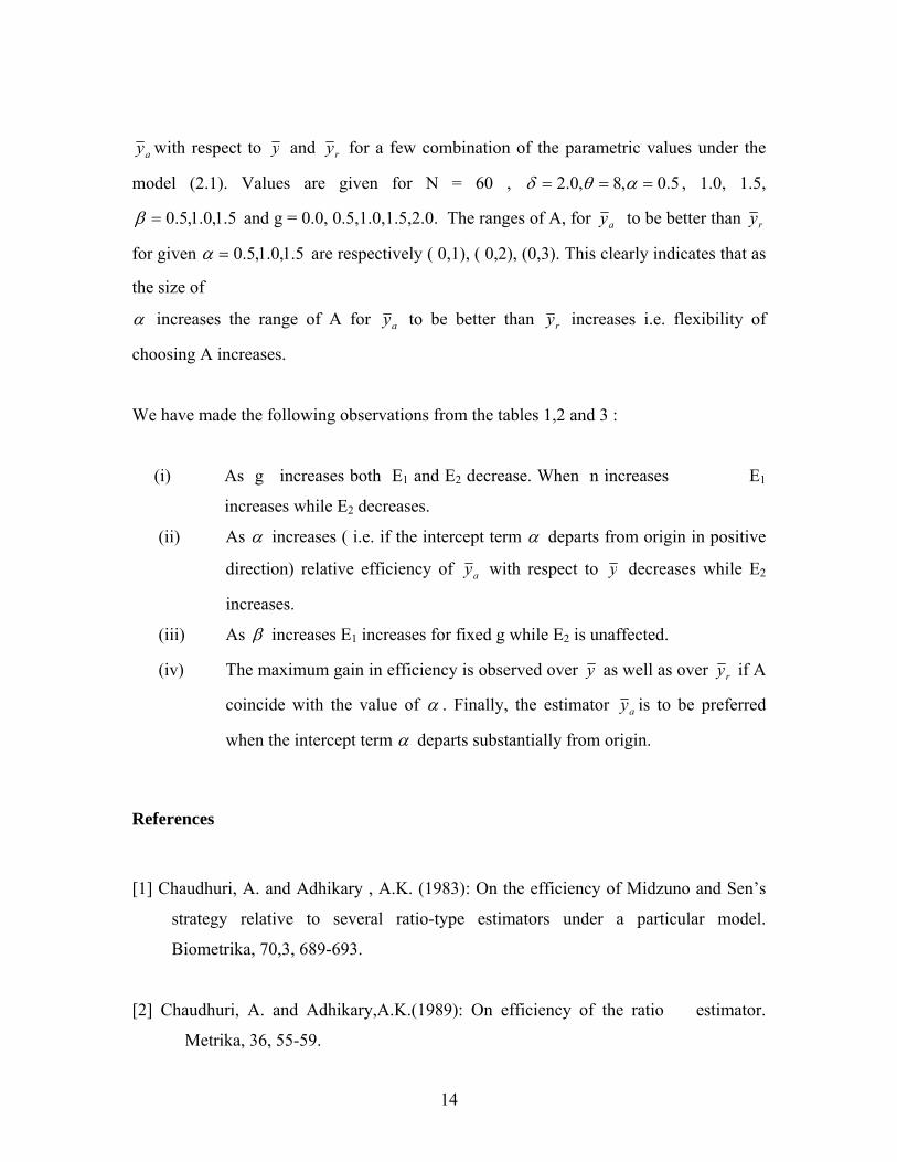
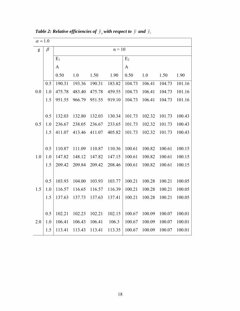
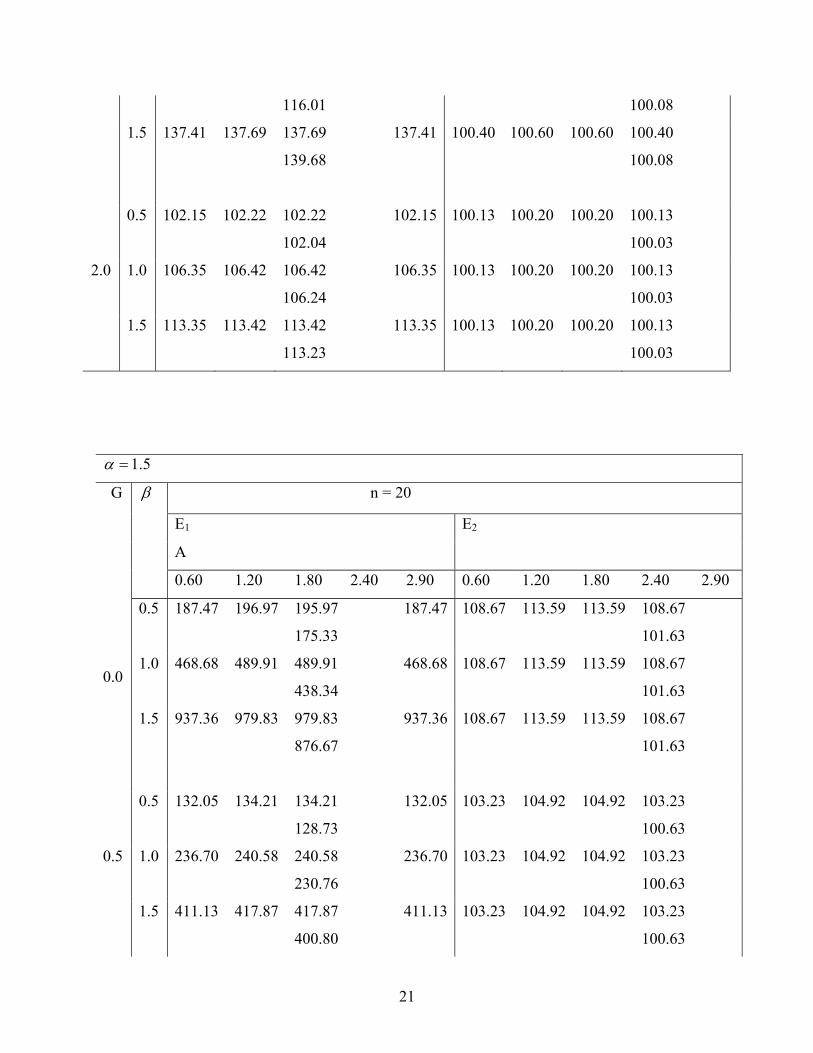
model (2.1). Values are given for N = 60 , 5.0,8,0.2 === αθδ , 1.0, 1.5,

5.1,0.1,5.0=β and g = 0.0, 0.5,1.0,1.5,2.0. The ranges of A, for ay to be better than ry

for given 5.1,0.1,5.0=α are respectively ( 0,1), ( 0,2), (0,3). This clearly indicates that as

the size of

α increases the range of A for ay to be better than ry increases i.e. flexibility of

choosing A increases.

We have made the following observations from the tables 1,2 and 3 :

(i) As g increases both E1 and E2 decrease. When n increases E1

increases while E2 decreases.

(ii) As α increases ( i.e. if the intercept term α departs from origin in positive

direction) relative efficiency of ay with respect to y decreases while E2

increases.

(iii) As β increases E1 increases for fixed g while E2 is unaffected.

(iv) The maximum gain in efficiency is observed over y as well as over ry if A

coincide with the value of α . Finally, the estimator ay is to be preferred

when the intercept term α departs substantially from origin.

References

[1] Chaudhuri, A. and Adhikary , A.K. (1983): On the efficiency of Midzuno and Sen’s

strategy relative to several ratio-type estimators under a particular model.

Biometrika, 70,3, 689-693.

[2] Chaudhuri, A. and Adhikary,A.K.(1989): On efficiency of the ratio estimator.

Metrika, 36, 55-59.

15

[3] Durbin, J. (1959): A note on the application of Quenouille’s method of bias reduction

in estimation of ratios. Biometrika,46,477-480.

[4] Rao, J.N.K. and Webster , J.T. (1966): On two methods of bias reduction in

estimation of ratios. Biometrika, 53, 571-577.

[5] Rao, P.S.R.S. (1968): On three procedures of sampling from finite populations.

Biometrika, 55,2,438-441.

[6] Shah , D.N. and Gupta, M. R. (1987): An efficiency comparison of dual to ratio and

product estimators. Commun. Statist. –Theory meth. 16 (3) , 693-703.

[7] Srivenkataramana, T. and Tracy , D.S. (1986) : Transformations after sampling.

Statistics, 17,4,597-608.

16

Table 1: Relative efficiencies of ay with respect to y and Γy

5.0=α

g β n = 10

E1 E2

A A

0.30 0.60 0.90 0.30 0.60 0.90

0.5 192.86 193.23 191.40 101.34 101.54 100.57

1.0 482.16 483.16 478.09 101.34 101.54 100.57 0.0

1.5 964.32 966.17 956.98 101.34 101.54 100.57

0.5 132.67 132.77 132.30 100.49 100.56 100.21

0.5 1.0 237.82 237.99 237.16 100.49 100.56 100.21

1.5 413.08 413.36 411.93 100.49 100.56 100.21

0.5 111.06 111.08 110.95 10.17 100.19 100.07

1.0 1.0 148.08

148.11 147.93 10.17 100.19 100.07

1.5 209.78 209.83 209.57 10.17 100.19 100.07

0.5 103.99 104.00 103.96 100.06 100.07 100.03

1.5 1.0 116.64 116.65 116.60 100.06 100.07 100.03

1.5 137.71 137.72 137.66 100.06 100.07 100.03

0.5 102.23 102.23 102.22 100.02 100.02 100.01

2.0 1.0 106.43 106.43 106.42 100.02 100.02 100.01

1.5 113.43 113.43 113.42 100.02 100.02 100.01

17

5.0=α

g β n = 20

E1 E2

A A

0.30 0.60 0.90 0.30 0.60 0.90

0.5 196.58 196.96 195.11 103.33 101.52 100.56

1.0 491.46 492.39 487.77 103.33 101.52 100.56 0.0

1.5 982.92 984.39 975.53 103.33 101.52 100.56

0.5 134.37 134.46 134.46 100.48 100.55 100.20

0.5 1.0 240.86 241.02 240.02 100.48 100.55 100.20

1.5 418.35 418.63 417.20 100.48 100.55 100.20

0.5 111.76 111.79 111.65 100.17 100.19 100.07

1.0 1.0 149.01 149.05 148.87 100.17 100.19 100.07

1.5 211.10 211.16 210.90 100.17 100.19 100.07

0.5 104.00 104.00 103.96 100.06 100.07 100.02

1.5 1.0 116.64 116.65 116.60 100.06 100.07 100.02

1.5 137.71 137.73 137.67 100.06 100.07 100.02

0.5 101.60 101.60 101.58 100.02 100.02 100.01

2.0 1.0 105.77 105.77 105.76 100.02 100.02 100.01

1.5 112.73 112.73 112.73 100.02 100.02 100.01

18

Table 2: Relative efficiencies of ay with respect to y and ry

0.1=α

g β n = 10

E1 E2

A A

0.50 1.0 1.50 1.90 0.50 1.0 1.50 1.90

0.5 190.31 193.36 190.31 183.82 104.73 106.41 104.73 101.16

1.0 475.78 483.40 475.78 459.55 104.73 106.41 104.73 101.16 0.0

1.5 951.55 966.79 951.55 919.10 104.73 106.41 104.73 101.16

0.5 132.03 132.80 132.03 130.34 101.73 102.32 101.73 100.43

0.5 1.0 236.67 238.05 236.67 233.65 101.73 102.32 101.73 100.43

1.5 411.07 413.46 411.07 405.82 101.73 102.32 101.73 100.43

0.5 110.87 111.09 110.87 110.36 100.61 100.82 100.61 100.15

1.0 1.0 147.82 148.12 147.82 147.15 100.61 100.82 100.61 100.15

1.5 209.42 209.84 209.42 208.46 100.61 100.82 100.61 100.15

0.5 103.93 104.00 103.93 103.77 100.21 100.28 100.21 100.05

1.5 1.0 116.57 116.65 116.57 116.39 100.21 100.28 100.21 100.05

1.5 137.63 137.73 137.63 137.41 100.21 100.28 100.21 100.05

0.5 102.21 102.23 102.21 102.15 100.67 100.09 100.07 100.01

2.0 1.0 106.41 106.43 106.41 106.3 100.67 100.09 100.07 100.01

1.5 113.41 113.43 113.41 113.35 100.67 100.09 100.07 100.01

19

0.1=α

g β n = 20

E1 E2

A A

0.50 1.0 1.50 1.90 0.50 1.0 1.50 1.90

0.5 194.01 197.08 194.01 187.47 104.67 106.33 104.67 101.14

1.0 485.03 492.70 485.03 468.68 104.67 106.33 104.67 101.14 0.0

1.5 970.06 985.40 970.06 937.36 104.67 106.33 104.67 101.14

0.5 133.73 134.49 133.73 132.05 101.70 102.28 101.70 100.08

0.5 1.0 239.71 241.08 239.71 236.71 101.70 102.28 101.70 100.08

1.5 416.35 418.73 416.35 411.13 101.70 102.28 101.70 100.08

0.5 111.07 111.08 111.07 111.08 100.60 100.80 100.60 100.15

1.0 1.0 148.77 149.06 148.77 148.11 100.60 100.80 100.60 100.15

1.5 210.75 211.17 210.75 209.82 100.60 100.80 100.60 100.15

0.5 103.94 104.01 103.94 103.78 100.20 100.27 100.20 100.05

1.5 1.0 116.57 116.65 116.57 116.40 100.20 100.27 100.20 100.05

1.5 137.64 137.73 137.64 137.42 100.20 100.27 100.20 100.05

0.5 101.58 101.60 101.58 101.52 100.07 100.09 100.07 100.01

2.0 1.0 105.75 105.77 105.75 105.70 100.07 100.09 100.07 100.01

1.5 112.71 112.73 112.71 112.65 100.07 100.09 100.07 100.01

20

Table 3: Relative efficiencies of ay with respect to y and ry

5.1=α

g β n = 10

E1 E2

A A

0.60 1.20 1.80 2.40 2.90 0.60 1.20 1.80 2.40 2.90

0.5 183.82 192.25 192.25 183.82

171.79

108.77 113.76 113.76 108.77

101.65

1.0 459.55 480.62 480.62 459.55

429.47

108.77 113.76 113.76 108.77

101.65 0.0

1.5 919.10 961.25 961.25 919.10

858.94

108.77 113.76 113.76 108.77

101.65

0.5 130.34 132.52 132.52 130.34

127.01

103.29 105.01 105.01 103.29

100.64

0.5 1.0 233.64 237.55 237.55 233.65

227.67

103.29 105.01 105.01 103.29

100.64

1.5 405.82 412.60 412.60 405.82

395.44

103.29 105.01 105.01 103.29

100.64

0.5 110.36 111.01 111.01 110.36

109.34

101.17 101.77 101.77 101.17

100.23

1.0 1.0 147.15 148.02 148.02 147.15

147.79

101.17 101.77 101.77 101.17

100.23

1.5 208.46 209.69 209.69 208.46

206.53

101.17 101.77 101.77 101.17

100.23

0.5 103.77 103.98 103.98 103.77

103.44

100.40 100.60 100.60 100.40

100.08

1.5 1.0 116.39 116.62 116.62 116.39 100.40 100.60 100.60 100.40

21

116.01 100.08

1.5 137.41 137.69 137.69 137.41

139.68

100.40 100.60 100.60 100.40

100.08

0.5 102.15 102.22 102.22 102.15

102.04

100.13 100.20 100.20 100.13

100.03

2.0 1.0 106.35 106.42 106.42 106.35

106.24

100.13 100.20 100.20 100.13

100.03

1.5 113.35 113.42 113.42 113.35

113.23

100.13 100.20 100.20 100.13

100.03

5.1=α

G β n = 20

E1 E2

A

0.60 1.20 1.80 2.40 2.90 0.60 1.20 1.80 2.40 2.90

0.5 187.47 196.97 195.97 187.47

175.33

108.67 113.59 113.59 108.67

101.63

1.0 468.68 489.91 489.91 468.68

438.34

108.67 113.59 113.59 108.67

101.63 0.0

1.5 937.36 979.83 979.83 937.36

876.67

108.67 113.59 113.59 108.67

101.63

0.5 132.05 134.21 134.21 132.05

128.73

103.23 104.92 104.92 103.23

100.63

0.5 1.0 236.70 240.58 240.58 236.70

230.76

103.23 104.92 104.92 103.23

100.63

1.5 411.13 417.87 417.87 411.13

400.80

103.23 104.92 104.92 103.23

100.63

22

0.5 111.08 111.72 111.72 111.08

110.08

101.14 101.72 101.72 101.14

100.23

1.0 1.0 148.11 148.96 148.96 148.11

146.77

101.14 101.72 101.72 101.14

100.23

1.5 209.82 211.02 211.02 209.82

207.92

101.14 101.72 101.72 101.14

100.23

0.5 103.78 103.98 103.98 103.78

103.46

100.39 100.58 100.58 100.39

100.08

1.5 1.0 116.40 116.62 116.62 116.40

116.40

100.39 100.58 100.58 100.39

100.08

1.5 137.43 137.70 137.70 137.43

137.00

100.39 100.58 100.58 100.39

100.08

0.5 101.53 101.59 101.59 101.53

101.42

100.13 100.19 100.19 100.03

100.03

2.0 1.0 105.70 105.77 105.77 105.70

105.59

100.13 100.19 100.19 100.03

100.03

1.5 112.65 112.72 112.72 112.65

112.54

100.13 100.19 100.19 100.03

100.03

23

Empirical Study in Finite Correlation Coefficient in Two Phase Estimation

M. Khoshnevisan

Griffith University, Griffith Business School

Australia

F. Kaymarm

Massachusetts Institute of Technology

Department of Mechanical Engineering, USA

H. P. Singh, R Singh

Vikram University

Department of Mathematics and Statistics, India

F. Smarandache

University of New Mexico

Department of Mathematics, Gallup, USA.

Abstract

This paper proposes a class of estimators for population correlation coefficient

when information about the population mean and population variance of one of the

variables is not available but information about these parameters of another variable

(auxiliary) is available, in two phase sampling and analyzes its properties. Optimum

estimator in the class is identified with its variance formula. The estimators of the class

involve unknown constants whose optimum values depend on unknown population

parameters.Following (Singh, 1982) and (Srivastava and Jhajj, 1983), it has been shown

that when these population parameters are replaced by their consistent estimates the

resulting class of estimators has the same asymptotic variance as that of optimum

24

estimator. An empirical study is carried out to demonstrate the performance of the

constructed estimators.

Keywords: Correlation coefficient, Finite population, Auxiliary information, Variance.

2000 MSC: 92B28, 62P20

1. Introduction

Consider a finite population U= {1,2,..,i,..N}. Let y and x be the study and auxiliary

variables taking values yi and xi respectively for the ith unit. The correlation coefficient

between y and x is defined by

yxρ = Syx /(SySx) (1.1)

where

( ) ( )( )XxYyNS i

N

iiyx −−−= ∑

=

−

1

11 , ( ) ( )∑=

− −−=N

iix XxNS

1

212 1 , ( ) ( )∑=

− −−=N

iiy YyNS

1

212 1 ,

∑=

−=N

iixNX

1

1 , ∑=

−=N

iiyNY

1

1 .

Based on a simple random sample of size n drawn without replacement,

(xi , yi), i = 1,2,…,n; the usual estimator of yxρ is the corresponding sample correlation

coefficient :

r= syx /(sxsy) (1.2)

where ( ) ( )( )xxyyns i

n

iiyx −−−= ∑

=

−

1

11 , ( ) ( )∑=

− −−=n

iix xxns

1

212 1

( ) ( )∑=

− −−=n

iiy yyns

1

212 1 , ∑=

−=n

iiyny

1

1 , ∑=

−=n

iixnx

1

1 .

The problem of estimating yxρ has been earlier taken up by various authors including

(Koop, 1970), (Gupta et. al., 1978, 1979), (Wakimoto, 1971), (Gupta and Singh, 1989),

(Rana, 1989) and (Singh et. al., 1996) in different situations. (Srivastava and Jhajj, 1986)

have further considered the problem of estimating yxρ in the situations where the

25

information on auxiliary variable x for all units in the population is available. In such

situations, they have suggested a class of estimators for yxρ which utilizes the known

values of the population mean X and the population variance 2xS of the auxiliary variable

x.

In this paper, using two – phase sampling mechanism, a class of estimators for

yxρ in the presence of the available knowledge ( Z and 2zS ) on second auxiliary variable z

is considered, when the population mean X and population variance 2xS of the main

auxiliary variable x are not known.

2. The Suggested Class of Estimators

In many situations of practical importance, it may happen that no information is

available on the population mean X and population variance 2xS , we seek to estimate the

population correlation coefficient yxρ from a sample ‘s’ obtained through a two-phase

selection. Allowing simple random sampling without replacement scheme in each phase,

the two- phase sampling scheme will be as follows:

(i) The first phase sample ∗s ( )Us ⊂∗ of fixed size 1n , is drawn to observe only x in

order to furnish a good estimates of X and 2xS .

(ii) Given ∗s , the second- phase sample s ( )∗⊂ ss of fixed size n is drawn to

observe y only.

Let

( )∑∈

=si

ixnx 1 , ( )∑∈

=si

iyny 1 , ( )∑∗∈

∗ =si

ixnx 11 , ( ) ( )∑∈

− −−=si

ix xxns 212 1 ,

( ) ( )∑∗∈

∗−∗ −−=si

ix xxns21

12 1 .

We write ∗= xxu , 22 ∗= xx ssv . Whatever be the sample chosen let (u,v) assume values in

a bounded closed convex subset, R, of the two-dimensional real space containing the

point (1,1). Let h (u, v) be a function of u and v such that

h(1,1)=1 (2.1)

and such that it satisfies the following conditions:

26

1. The function h (u,v) is continuous and bounded in R.

2. The first and second partial derivatives of h(u,v) exist and are continuous and

bounded in R.

Now one may consider the class of estimators of yxρ defined by

),(ˆ vuhrhd =ρ (2.2)

which is double sampling version of the class of estimators

),(~ ∗∗= vufrrt

Suggested by (Srivastava and Jhajj, 1986), where Xxu =∗ , 22xx Ssv =∗ and ( )2, xSX are

known.

Sometimes even if the population mean X and population variance 2xS of x are

not known, information on a cheaply ascertainable variable z, closely related to x but

compared to x remotely related to y, is available on all units of the population. This type

of situation has been briefly discussed by, among others, (Chand, 1975), (Kiregyera,

1980, 1984).

Following (Chand, 1975) one may define a chain ratio- type estimator for yxρ as

⎟⎟⎠

⎞⎜⎜⎝

⎛⎟⎟⎠

⎞⎜⎜⎝

⎛⎟⎟⎠

⎞⎜⎜⎝

⎛⎟⎟⎠

⎞⎜⎜⎝

⎛=

∗

∗

∗

∗

2

2

2

2

1ˆz

z

x

xd s

Sss

zZ

xxrρ (2.3)

where the population mean Z and population variance 2zS of second auxiliary variable z are

known, and

( )∑∗∈

∗ =si

iznz 11 , ( ) ( )∑∗∈

∗−∗ −−=si

iz zzns21

12 1

are the sample mean and sample variance of z based on preliminary large sample s* of

size n1 (>n).

The estimator d1ρ̂ in (2.3) may be generalized as

4321

2

2

2

2

2ˆαααα

ρ ⎟⎟⎠

⎞⎜⎜⎝

⎛⎟⎟⎠

⎞⎜⎜⎝

⎛⎟⎟⎠

⎞⎜⎜⎝

⎛⎟⎠⎞

⎜⎝⎛=

∗∗

∗∗z

z

x

xd S

sZz

ss

xxr (2.4)

27

where si 'α (i=1,2,3,4) are suitably chosen constants.

Many other generalization of d1ρ̂ is possible. We have, therefore, considered a

more general class of yxρ from which a number of estimators can be generated.

The proposed generalized estimators for population correlation coefficient yxρ is

defined by

),,,(ˆ awvutrtd =ρ (2.5)

where Zzw ∗= , 22zz Ssa ∗= and t(u,v,w,a) is a function of (u,v,w,a) such that

t (1,1,1,1)=1 (2.6)

Satisfying the following conditions:

(i) Whatever be the samples (s* and s) chosen, let (u,v,w,a) assume values in a closed

convex subset S, of the four dimensional real space containing the point P=(1,1,1,1).

(ii) In S, the function t(u,v,w,a) is continuous and bounded.

(iii) The first and second order partial derivatives of t(u,v,w, a) exist and are

continuous and bounded in S

To find the bias and variance of tdρ̂ we write

)1(),1(),1(),1(

)1(),1(),1(),1(*4

22**3

**2

22*

222*

11122

syxyxzzxx

xxyy

eSseSseZzeSs

eSseXxeXxeSs

+=+=+=+=

+=+=+=+= ∗

such that E(e0) =E (e1)=E(e2)=E(e5)=0 and E(ei*) = 0 ∀ i = 1,2,3,4,

and ignoring the finite population correction terms, we write to the first degree of

approximation

28

( ) ( ) ( ) ( ) ( ) ( )( ) ( ) ( ) ( ) ( )( ) ( ){ } ( ) ( )( ) ( ) ( ) ( ) ( )( ) ( ) ( ) ( ){ }( ) ( ) ( )( ) ( ) ( ) ( )( ) ( ) ( )( ) ( ) ( )( ) ( ) ( ) ( ) ( )( ) ( ){ } ( )( ) ( ) ( ) ( ){ }( ) ( ) ( )( ) ( ){ } .1

,,

,1,1

,,1

,1,,1

,,

,,,

,,,

,,,

,1,1

,,1,1

,,,1

,1,,1

,1,,,1

111254

111153100343

113052102242

10213213052

102242102132104022

112051101241

131103021103021

12051101241131

1030210302112

11

31050120240

12013012202022020

121010210102

22025

10042

4122

310402

2

040221

221

221400

20

neeE

nCeeEnCeeE

neeEneeE

nCeeEneeE

neeEnCeeEneeE

nCeeEnCeeE

nCCeeEnCeeEnCeeE

nCeeEnCeeEnCCeeE

nCeeEnCeeEnCeeE

neeEneeE

nCeeEneeEneeE

nCeeEnCeeEneE

neEnCeEneE

neEnCeEnCeEneE

yx

yxzz

yx

zyx

z

yxxx

zxxzxx

yxxxzxxz

xxx

yx

z

xxyx

z

xx

−=

==

−=−=

=−=

−==−=

==

===

===

===

−=−=

=−=−=

==−=

−==−=

−===−=

∗

∗∗∗

∗∗∗

∗∗

∗∗∗

∗∗∗

∗∗∗∗∗

∗∗

∗∗

∗

∗∗

∗

∗∗∗

∗

ρδ

ρδδ

ρδδ

δρδ

δδδ

ρδδ

ρδδ

ρδδρ

δδ

ρδδ

δδδ

δδρδ

δδ

δδ

where

( )2/002

2/020

2/200

mqppqmpqm μμμμδ = , ( ) ( ) ( ) ( )∑

=

−−−=N

i

mi

qi

pipqm ZzXxYyN

11μ , (p,q,m) being

non-negative integers.

To find the expectation and variance of tdρ̂ , we expand t(u,v,w,a) about the point

P= (1,1,1,1) in a second- order Taylor’s series, express this value and the value of r in

terms of e’s . Expanding in powers of e’s and retaining terms up to second power, we

have

E( tdρ̂ )= ( )1−+ noyxρ (2.7)

which shows that the bias of tdρ̂ is of the order n-1and so up to order n-1 , mean square

error and the variance of tdρ̂ are same.

Expanding ( )2ˆ yxtd ρρ − , retaining terms up to second power in e’s, taking

expectation and using the above expected values, we obtain the variance of tdρ̂ to the

first degree of approximation, as

29

)]()(2)()(2)()()(

)()()1()()()1()()[/(

)]()(2)()()()1()()[/()()ˆ(

4300321030432

124004

23

222040

21

21

2

210302122040

21

22

PtPtCPtPtCPtFPDtPBt

PAtPtPtCPtPtCn

PtPtCPBtPAtPtPtCnrVarVar

zx

zxyx

xxyxtd

δδ

δδρ

δδρρ

−+++

−−−−−−+−

+−−−++=

(2.8)

where t1(P), t2(P), t3(P)and t4(P) respectively denote the first partial derivatives of

t(u,v,w,a) white respect to u,v,w and a respectively at the point P= (1,1,1,1),

Var(r)= ( ) }]/){()2)(4/1(/)[/( 3101302204000402

2202

yxyxyx n ρδδδδδρδρ +−+++ (2.9)

)}/(2{,)}/(2{

)},/(2{,)}/(2{

112022202111021201

130040220120030210

yxzyx

yxxyx

FCD

BCA

ρδδδρδδδ

ρδδδρδδδ

−+=−+=

−+=−+=

Any parametric function t(u,v,w,a) satisfying (2.6) and the conditions (1) and (2) can

generate an estimator of the class(2.5).

The variance of tdρ̂ at (2.6) is minimized for

( )[ ]( )

( )( )

( )[ ]( )

( )( ) ⎪

⎪⎪⎪⎪

⎭

⎪⎪⎪⎪⎪

⎬

⎫

=−−

−=

=−−

−−=

=−−

−=

=−−

−−=

(say),12

)(

(say),12

1)(

(say),12

)(

(say),12

1)(

2003004

2003

2

4

2030004

2003004

3

2030040

2030

2

2

2030040

2030040

1

δδδδ

γδδδδ

βδδδ

αδδδδ

z

zz

z

z

x

xx

x

x

CCDFC

Pt

CCFD

Pt

CCABC

Pt

CCBA

Pt

(2.10)

Thus the resulting (minimum) variance of tdρ̂ is given by

⎥⎥⎦

⎤

⎢⎢⎣

⎡

−−−

+−

−−

−+−−=

)1(4})/{(

4)/(

])1(4})/{(

4[)11()()ˆ(.min

2003004

2003

2

2

12

2030040

2030

2

22

1

δδδ

ρ

δδδ

ρρ

FCDCDn

BCACA

nnrVarVar

z

zyx

x

xyxtd

(2.11)

30

It is observed from (2.11) that if optimum values of the parameters given by

(2.10) are used, the variance of the estimator tdρ̂ is always less than that of r as the last

two terms on the right hand sides of (2.11) are non-negative.

Two simple functions t(u,v,w,a) satisfying the required conditions are

t(u,v,w,a)= 1+ )1()1()1()1( 4321 −+−+−+− awvu αααα

4321),,,( αααα awvuawvut =

and for both these functions t1(P) = 1α , t2 (P) = 2α , t3 (P) = 3α and t4 (P) = 4α . Thus one

should use optimum values of 1α , 2α , 3α and 4α in tdρ̂ to get the minimum variance. It is

to be noted that the estimated tdρ̂ attained the minimum variance only when the optimum

values of the constants iα (i=1,2,3,4), which are functions of unknown population

parameters, are known. To use such estimators in practice, one has to use some guessed

values of population parameters obtained either through past experience or through a

pilot sample survey. It may be further noted that even if the values of the constants used

in the estimator are not exactly equal to their optimum values as given by (2.8) but are

close enough, the resulting estimator will be better than the conventional estimator, as has

been illustrated by (Das and Tripathi, 1978, Sec.3).

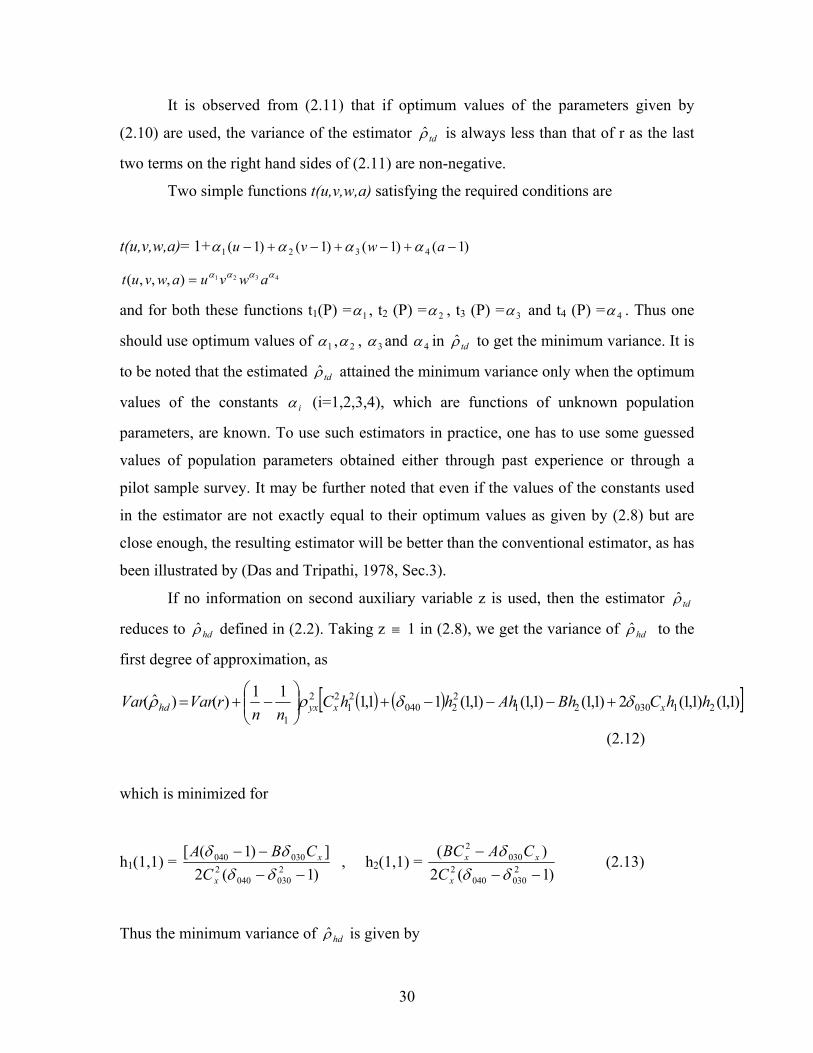
If no information on second auxiliary variable z is used, then the estimator tdρ̂

reduces to hdρ̂ defined in (2.2). Taking z ≡ 1 in (2.8), we get the variance of hdρ̂ to the

first degree of approximation, as

( ) ( )[ ])1,1()1,1(2)1,1()1,1()1,1(11,111)()ˆ( 210302122040

21

22

1hhCBhAhhhC

nnrVarVar xxyxhd δδρρ +−−−+⎟⎟

⎠

⎞⎜⎜⎝

⎛−+=

(2.12)

which is minimized for

h1(1,1) = )1(2

])1([2030040

2030040

−−−−δδδδ

x

x

CCBA

, h2(1,1) = )1(2

)(2030040

2030

2

−−−

δδδ

x

xx

CCABC

(2.13)

Thus the minimum variance of hdρ̂ is given by

31

min.Var( hdρ̂ )=Var(r) -(1

11nn

− ) 2yxρ [ 2

2

4 xCA +

)1(4}){(

2030040

2030

−−−

δδδ BCA x ] (2.14)

It follows from (2.11) and (2.14) that

min.Var( tdρ̂ )-min.Var( hdρ̂ )= ( )12 nyxρ [

)1(4}){(

4 2003004

2003

2

2

−−

−+

δδδ FCD

CD z

z

] (2.15)

which is always positive. Thus the proposed estimator tdρ̂ is always better than hdρ̂ .

3. A Wider Class of Estimators

In this section we consider a class of estimators of yxρ wider than ( 2.5) given by

gdρ̂ =g(r,u,v,w,a) (3.1)

where g(r,u,v,w,a) is a function of r,u,v, w,a and such that

g( ρ ,1,1,1,1)= tdρ̂ and )1,1,1,(

)(

ρ⎥⎦⎤

⎢⎣⎡∂⋅∂

rg = 1

Proceeding as in section 2, it can easily be shown, to the first order of approximation, that

the minimum variance of gdρ̂ is same as that of tdρ̂ given in (2.11).

It is to be noted that the difference-type estimator

rd= r + 1α (u-1) + 2α (v-1) + 3α (w-1) + 4α (a-1), is a particular case of gdρ̂ , but it is

not the member of tdρ̂ in (2.5).

4. Optimum Values and Their Estimates

The optimum values t1(P) = α , t2(P) = β , t3(P) = γ and t4(P) =δ given at

(2.10) involves unknown population parameters. When these optimum values are

substituted in (2.5) , it no longer remains an estimator since it involves unknown

(α , β ,γ ,δ ), which are functions of unknown population parameters, say,, pqmδ (p, q,m=

0,1,2,3,4), Cx, Cz and yxρ itself. Hence it is advisable to replace them by their consistent

estimates from sample values. Let ( δγβα ˆ,ˆ,ˆ,ˆ ) be consistent estimators of t1(P),t2(P),

t3(P) and t4(P) respectively, where

32

)1ˆˆ(ˆ2]ˆˆˆ)1ˆ(ˆ[ˆ)(ˆ

2030040

2030040

1−−

−−==

δδδδ

αx

x

CCBA

Pt , [ ])1ˆˆ(ˆ2

ˆˆˆˆˆˆ)(ˆ

2030040

2030

2

2−−

−==

δδδ

βx

xx

CCACB

Pt ,

)1ˆˆ(ˆ2]ˆˆˆ)1ˆ(ˆ[ˆ)(ˆ

2003004

2003004

3−−

−−==

δδδδ

γz

z

CCFD

Pt , [ ])1ˆˆ(ˆ2

ˆˆˆˆˆˆ)(ˆ

2003004

2003

2

4−−

−==

δδδ

δz

zz

CCDFC

Pt ,

(4.1)

with

xCrA ˆ)]/ˆ(2ˆˆ[ˆ120030210 δδδ −+= , )]/ˆ(2ˆˆ[ˆ

130040220 rB δδδ −+= ,

zCrD ˆ)]/ˆ(2ˆˆ[ˆ111021201 δδδ −+= , )]/ˆ(2ˆˆ[ˆ

112022202 rF δδδ −+= ,

xsC xx /ˆ = , zsC zz /ˆ = , ( )2/002

2/020

2/200 ˆˆˆˆˆ mqp

pqmpqm μμμμδ =

( ) ( ) ( ) ( )∑=

−−−=n

i

mi

qi

pipqm zzxxyyn

11μ̂

∑=

=n

iiznz

1

)/1( , ∑=

− −−=n

iix xxns

1

212 )()1( , ∑=

=n

iixnx

1

)/1( ,

2

1

12 )()1(),/( ∑=

− −−==n

iiyxyyx yynssssr , ∑

=

− −−=n

iiz zxns

1

212 )()1( .

We then replace (α , β ,γ ,δ ) by ( δγβα ˆ,ˆ,ˆ,ˆ ) in the optimum tdρ̂ resulting in the estimator

∗tdρ̂ say, which is defined by

)ˆ,ˆ,ˆ,ˆ,,,,(ˆ ** δγβαρ awvutrtd = , (4.2)

where the function t*(U), U= ( δγβα ˆ,ˆ,ˆ,ˆ,,,, awvu ) is derived from the the function

t(u,v,w,a) given at (2.5) by replacing the unknown constants involved in it by the

consistent estimates of optimum values. The condition (2.6) will then imply that

t*(P*) = 1 (4.3)

where P* = (1,1,1,1, α , β ,γ ,δ )

We further assume that

33

α=⎥⎦⎤

∂∂

== *

)(**)(1PUu

UtPt , β=⎥⎦⎤

∂∂

== *

)(**)(2PUv

UtPt

γ=⎥⎦⎤

∂∂

== *

)(**)(3PUw

UtPt , δ=⎥⎦⎤

∂∂

== *

)(**)(4PUa

UtPt (4.4)

οα

=⎥⎦⎤

∂∂

== *ˆ

)(**)(5PU

UtPt οβ

=⎥⎥⎦

⎤

∂

∂=

= *ˆ

)(**)(6PU

UtPt

ογ

=⎥⎦

⎤∂

∂=

= *ˆ)(**)(7

PU

UtPt οδ

=⎥⎦

⎤∂

∂=

= *ˆ)(**)(8

PU

UtPt

Expanding t*(U) about P*= (1,1,1,1, α , β ,γ ,δ ), in Taylor’s series, we have

( ) ( ) terms]ordersecond)()ˆ(ˆ)()ˆ(

)()ˆ()()1()()1()()1()()1()([ˆ**

87**

6

**5

**4

**3

**2

**1

***

+−+−+−+

−+−+−+−+−+=∗∗ PtPtPt

PtPtaPtwPtvPtuPtrtd

δδγγββ

ααρ

(4.5)

Using (4.4) in (4.5) we have

terms]ordersecond)1()1()1()1(1[ˆ * +−+−+−+−+= δγβαρ awvurtd (4.6)

Expressing (4.6) in term of e’s squaring and retaining terms of e’s up to second degree,

we have

2*4

*3

*22

*11205

22* ])()()2(21[)ˆ( eeeeeeeeeyxyxtd δγβαρρρ ++−+−+−−=− (4.7)

Taking expectation of both sides in (4.7), we get the variance of ∗tdρ̂ to the first degree of

approximation, as

34

⎥⎥⎦

⎤

⎢⎢⎣

⎡

−−

−++

⎥⎥⎦

⎤

⎢⎢⎣

⎡

−−

−+−−=

)1(4})/{(

4)/(

)1(4})/{(

4)11()()ˆ(

2003004

2003

2

2

12

2030040

2030

2

22

1

*

δδδ

ρ

δδδ

ρρ

FCDCDn

BCACA

nnrVarVar

z

zyx

x

xyxtd

(4.8)

which is same as (2.11), we thus have established the following result.

Result 4.1: If optimum values of constants in (2.10) are replaced by their consistent

estimators and conditions (4.3) and (4.4) hold good, the resulting estimator *ˆ tdρ has the

same variance to the first degree of approximation, as that of optimum tdρ̂ .

Remark 4.1: It may be easily examined that some special cases:

(i) ,ˆ ˆˆˆˆ*1

δγβαρ awvurtd = (ii) )}1(ˆ)1(ˆ1{)}1(ˆ)1(ˆ1{ˆ *

2−−−−

−+−+=

avwurtd

δβγαρ

(iii) )]1(ˆ)1(ˆ)1(ˆ)1(ˆ1[ˆ *3 −+−+−+−+= awuurtd δγβαρ

(iv) 1*4 )]1(ˆ)1(ˆ)1(ˆ)1(ˆ1[ˆ −−−−−−−−−= awuurtd δγβαρ

of *ˆ tdρ satisfy the conditions (4.3) and (4.4) and attain the variance (4.8).

Remark 4.2: The efficiencies of the estimators discussed in this paper can be compared

for fixed cost, following the procedure given in (Sukhatme et. al., 1984).

5. Empirical Study

To illustrate the performance of various estimators of population

correlation coefficient, we consider the data given in (Murthy, 1967, p. 226]. The

variates are:

y=output, x=Number of Workers, z =Fixed Capital

N=80, n=10, n1 =25 ,

35

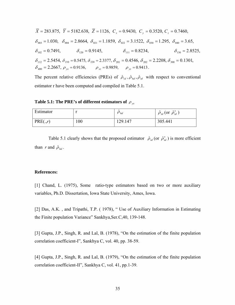
,875.283=X ,638.5182=Y ,1126=Z ,9430.0=xC ,3520.0=yC ,7460.0=zC

,030.1003 =δ ,8664.2004 =δ ,1859.1021 =δ ,1522.3022 =δ ,295.1030 =δ ,65.3040 =δ

,7491.0102 =δ ,9145.0120 =δ ,8234.0111 =δ ,8525.2130 =δ

,5454.2112 =δ ,5475.0210 =δ ,3377.2220 =δ ,4546.0201 =δ ,2208.2202 =δ ,1301.0300 =δ,2667.2400 =δ ,9136.0=yxρ ,9859.0=xzρ 9413.0=yzρ .

The percent relative efficiencies (PREs) of d1ρ̂ , hdρ̂ , tdρ̂ with respect to conventional

estimator r have been computed and compiled in Table 5.1.

Table 5.1: The PRE’s of different estimators of yxρ

Estimator r hdρ̂ tdρ̂ (or ∗

tdρ̂ )

PRE(.,r) 100 129.147 305.441

Table 5.1 clearly shows that the proposed estimator tdρ̂ (or ∗tdρ̂ ) is more efficient

than r and hdρ̂ .

References:

[1] Chand, L. (1975), Some ratio-type estimators based on two or more auxiliary

variables, Ph.D. Dissertation, Iowa State University, Ames, Iowa.

[2] Das, A.K. , and Tripathi, T.P. ( 1978), “ Use of Auxiliary Information in Estimating

the Finite population Variance” Sankhya,Ser.C,40, 139-148.

[3] Gupta, J.P., Singh, R. and Lal, B. (1978), “On the estimation of the finite population

correlation coefficient-I”, Sankhya C, vol. 40, pp. 38-59.

[4] Gupta, J.P., Singh, R. and Lal, B. (1979), “On the estimation of the finite population

correlation coefficient-II”, Sankhya C, vol. 41, pp.1-39.

36

[5] Gupta, J.P. and Singh, R. (1989), “Usual correlation coefficient in PPSWR sampling”,

Journal of Indian Statistical Association, vol. 27, pp. 13-16.

[6] Kiregyera, B. (1980), “A chain- ratio type estimators in finite population, double

sampling using two auxiliary variables”, Metrika, vol. 27, pp. 217-223.

[7] Kiregyera, B. (1984), “Regression type estimators using two auxiliary variables and

the model of double sampling from finite populations”, Metrika, vol. 31, pp. 215-226.

[8] Koop, J.C. (1970), “Estimation of correlation for a finite Universe”, Metrika, vol. 15,

pp. 105-109.

[9] Murthy, M.N. (1967), Sampling Theory and Methods, Statistical Publishing Society,

Calcutta, India.

[10] Rana, R.S. (1989), “Concise estimator of bias and variance of the finite population

correlation coefficient”, Jour. Ind. Soc., Agr. Stat., vol. 41, no. 1, pp. 69-76.

[11] Singh, R.K. (1982), “On estimating ratio and product of population parameters”,

Cal. Stat. Assoc. Bull., Vol. 32, pp. 47-56.

[12] Singh, S., Mangat, N.S. and Gupta, J.P. (1996), “Improved estimator of finite

population correlation coefficient”, Jour. Ind. Soc. Agr. Stat., vol. 48, no. 2, pp. 141-149.

[13] Srivastava, S.K. (1967), “An estimator using auxiliary information in sample

surveys. Cal. Stat. Assoc. Bull.”, vol. 16, pp. 121-132.

[14] Srivastava, S.K. and Jhajj, H.S. (1983), “A Class of estimators of the population

mean using multi-auxiliary information”, Cal. Stat. Assoc. Bull., vol. 32, pp. 47-56.

37

[15] Srivastava, S.K. and Jhajj, H.S. (1986), “On the estimation of finite population

correlation coefficient”, Jour. Ind. Soc. Agr. Stat., vol. 38, no. 1 , pp. 82-91.

[16] Srivenkataremann, T. and Tracy, D.S. (1989), “Two-phase sampling for selection

with probability proportional to size in sample surveys”, Biometrika, vol. 76, pp. 818-

821.

[17] Sukhatme, P.V., Sukhatme, B.V., Sukhatme, S. and Asok, C. ( 1984), “Sampling

Theory of Surveys with Applications”, Indian Society of Agricultural Statistics, New

Delhi.

[18] Wakimoto, K.(1971), “Stratified random sampling (III): Estimation of the

correlation coefficient”, Ann. Inst. Statist, Math, vol. 23, pp. 339-355.

38

MASS – Modified Assignment Algorithm in Facilities Layout Planning

Dr. Sukanto Bhattacharya

Department of Business Administration

Alaska Pacific University, AK 99508, USA

Dr. Florentin Smarandache

University of New Mexico

200 College Road, Gallup, USA

Dr. M. Khoshnevisan

School of Accounting & Finance

Griffith University, Australia

Abstract

In this paper we have proposed a semi-heuristic optimization algorithm for designing

optimal plant layouts in process-focused manufacturing/service facilities. Our proposed

algorithm marries the well-known CRAFT (Computerized Relative Allocation of

Facilities Technique) with the Hungarian assignment algorithm. Being a semi-heuristic

search, our algorithm is likely to be more efficient in terms of computer CPU engagement

time as it tends to converge on the global optimum faster than the traditional CRAFT

algorithm - a pure heuristic. We also present a numerical illustration of our algorithm.

Key Words: Facilities layout planning, load matrix, CRAFT, Hungarian assignment

algorithm

39

Introduction

The fundamental integration phase in the design of productive systems is the layout of

production facilities. A working definition of layout may be given as the arrangement of

machinery and flow of materials from one facility to another, which minimizes material-

handling costs while considering any physical restrictions on such arrangement. Usually

this layout design is either on considerations of machine-time cost and product

availability; thereby making the production system product-focused; or on considerations

of quality and flexibility; thereby making the production system process-focused. It is

natural that while product-focused systems are better off with a ‘line layout’ dictated by

available technologies and prevailing job designs, process-focused systems, which are

more concerned with job organization, opt for a ‘functional layout’. Of course, in reality

the actual facility layout often lies somewhere in between a pure line layout and a pure

functional layout format; governed by the specific demands of a particular production

plant. Since our present paper concerns only functional layout design for process-focused

systems, this is the only layout design we will discuss here.

The main goal to keep in mind is to minimize material handling costs - therefore the

departments that incur the most interdepartmental movement should be located closest to

one another. The main type of design layouts is Block diagramming, which refers to the

movement of materials in existing or proposed facility. This information is usually

provided with a from/to chart or load summary chart, which gives the average number of

units loads moved between departments. A load-unit can be a single unit, a pallet of

material, a bin of material, or a crate of material. The next step is to design the layout by

calculating the composite movements between departments and rank them from most

movement to least movement. Composite movement refers to the back-and-forth

movement between each pair of departments. Finally, trial layouts are placed on a grid

that graphically represents the relative distances between departments. This grid then

becomes the objective of optimization when determining the optimal plant layout.

We give a visual representation of the basic operational considerations in a process-

focused system schematically as follows:

40

Figure 1

In designing the optimal functional layout, the fundamental question to be addressed is

that of ‘relative location of facilities’. The locations will depend on the need for one pair

of facilities to be adjacent (or physically close) to each other relative to the need for all

other pairs of facilities to be similarly adjacent (or physically close) to each other.

Locations must be allocated based on the relative gains and losses for the alternatives and

seek to minimize some indicative measure of the cost of having non-adjacent locations of

facilities. Constraints of space prevents us from going into the details of the several

criteria used to determine the gains or losses from the relative location of facilities and

the available sequence analysis techniques for addressing the question; for which we refer

the interested reader to any standard handbook of production/operations management.

Computerized Relative Allocation of Facilities Technique (CRAFT)

CRAFT (Buffa, Armour and Vollman, 1964) is a computerized heuristic algorithm that

takes in load matrix of interdepartmental flow and transaction costs with a representation

of a block layout as the inputs. The block layout could either be an existing layout or; for

a new facility, any arbitrary initial layout. The algorithm then computes the departmental

locations and returns an estimate of the total interaction costs for the initial layout. The

governing algorithm is designed to compute the impact on a cost measure for two-way or

Updating skills and resources required for a particular process

Routing in-process items to the appropriate functional areas to facilitate processing

Establishing the right statistical process control mechanism

Process feedback

41

three-way swapping in the location of the facilities. For each swap, the various

interaction costs are computed afresh and the load matrix and the change in cost (increase

or decrease) is noted and stored in the RAM. The algorithm proceeds this way through all

possible combinations of swaps accommodated by the software. The basic procedure is

repeated a number of times resulting in a more efficient block layout every time till such

time when no further cost reduction is possible. The final block layout is then printed out

to serve as the basis for a detailed layout template of the facilities at a later stage. Since

its formulation, more powerful versions of CRAFT have been developed but these too

follow the same, basic heuristic routine and therefore tend to be highly CPU-intensive

(Khalil, 1973; Hicks and Cowan, 1976).

The basic computational disadvantage of a CRAFT-type technique is that one always has

got to start with an arbitrary initial solution (Carrie, 1980). This means that there is no

mathematical certainty of attaining the desired optimal solution after a given number of

iterations. If the starting solution is quite close to the optimal solution by chance, then the

final solution is attained only after a few iterations. However, as there is no guarantee that

the starting solution will be close to the global optimum, the expected number of

iterations required to arrive at the final solution tend to be quite large thereby straining

computing resources (Driscoll and Sangi, 1988).

In our present paper we propose and illustrate the Modified Assignment (MASS)

algorithm as an extension to the traditional CRAFT, to enable faster convergence to the

optimal solution. This we propose to do by marrying CRAFT technique with the

Hungarian assignment algorithm. As our proposed algorithm is semi-heuristic, it is likely

to be less CPU-intensive than any traditional, purely heuristic CRAFT-type algorithm.

42

The Hungarian assignment algorithm

A general assignment problem may be framed as a special case of the balanced

transportation problem with availability and demand constraints summing up to unity.

Mathematically, it has the following general linear programming form:

Minimize ΣΣ CijXij

Subject to ΣXij = 1, for each i, j = 1, 2 …n .

In words, the problem may be stated as assigning each of n individuals to n jobs so that

exactly one individual is assigned to each job in such a way as to minimize the total cost.

To ensure satisfaction of the basic requirements of the assignment problem, the basic

feasible solutions of the corresponding balanced transportation problem must be integer

valued. However, any such basic feasible solution will contain (2n – 1) variables out of

which (n – 1) variables will be zero thereby introducing a high level of degeneracy in the

solution making the usual solution technique of a transportation problem very inefficient.

This has resulted in mathematicians devising an alternative, more efficient algorithm for

solving this class of problems, which has come to be commonly known as the Hungarian

assignment algorithm. Basically, this algorithm draws from a simple theorem in linear

algebra which says that if a constant number is added to any row and/or column of the

cost matrix of an assignment-type problem, then the resulting assignment-type problem

has exactly the same set of optimal solutions as the original problem and vice versa.

Proof:

Let Ai and Bj (i, j = 1, 2 … n) be added to the ith row and/or jth column respectively of

the cost matrix. Then the revised cost elements are Cij* = Cij + Ai +Bj. The revised cost of

assignment is ΣΣCij*Xij = ΣΣ (Cij + Ai + Bj) Xij = ΣΣCijXij + ΣAi ΣXij + ΣBjΣXij. But by

the imposed assignment constraint ΣXij = 1 (for i, j = 1, 2 … n), we have the revised

43

cost as ΣΣCijXij + ΣAi + ΣBj i.e. the cost differs from the original by a constant. As the

revised costs differ from the originals by a constant, which is independent of the decision

variables, an optimal solution to one is also optimal solution to the other and vice versa.

This theorem can be used in two different ways to solve the assignment problem. First, if

in an assignment problem, some cost elements are negative, the problem may be

converted into an equivalent assignment problem by adding a positive constant to each of

the entries in the cost matrix so that they all become non-negative. Next, the important

thing to look for is a feasible solution that has zero assignment cost after adding suitable

constants to the rows and columns. Since it has been assumed that all entries are now

non-negative, this assignment must be the globally optimal one (Mustafi, 1996).

Given a zero assignment, a straight line is drawn through it (a horizontal line in case of a

row and a vertical line in case of a column), which prevents any other assignment in that

particular row/column. The governing algorithm then seeks to find the minimum number

of such straight lines, which would cover all the zero entries to avoid any redundancy.

Let us say that k such lines are required to cover all the zeroes. Then the necessary

condition for optimality is that number of zeroes assigned is equal to k and the sufficient

condition for optimality is that k is equal to n for an n x n cost matrix.

The MASS (Modified Assignment) algorithm

The basic idea of our proposed algorithm is to develop a systematic scheme to arrive at

the initial input block layout to be fed into the CRAFT program so that the program does

not have to start off from any initial (and possibly inefficient) solution. Thus, by

subjecting the problem of finding an initial block layout to a mathematical scheme, we in

effect reduce the purely heuristic algorithm of CRAFT to a semi-heuristic one. Our

proposed MASS algorithm follows the following sequential steps:

44

Step 1: We formulate the load matrix such that each entry lij represents the load carried

from facility i to facility j

Step 2: We insert lij = M, where M is a large positive number, into all the vacant cells of

the load matrix signifying that no inter-facility load transportation is required or possible

between the ith and jth vacant cells

Step 3: We solve the problem on the lines of a standard assignment problem using the

Hungarian assignment algorithm treating the load matrix as the cost matrix

Step 4: We draft the initial block layout trying to keep the inter-facility distance dij*

between the ith and jth assigned facilities to the minimum possible magnitude, subject to

the available floor area and architectural design of the shop floor

Step 5: We proceed using the CRAFT program to arrive at the optimal layout by

iteratively improving upon the starting solution provided by the Hungarian assignment

algorithm till the overall load function L = ΣΣ lijdij* subject to any particular bounds

imposed on the problem

The Hungarian assignment algorithm will ensure that the initial block layout is at least

very close to the global optimum if not globally optimal itself. Therefore the subsequent

CRAFT procedure will converge on the global optimum much faster starting from this

near-optimal initial input block layout and will be much less CPU-intensive that any

traditional CRAFT-type algorithm. Thus MASS is not a stand-alone optimization tool but

rather a rider on the traditional CRAFT that tries to ensure faster convergence to the

optimal block layout for process-focused systems, by making the search semi-heuristic.

We provide a numerical illustration of the MASS algorithm in the Appendix by designing

the optimal block layout of a small, single-storied, process-focused manufacturing plant

45

with six different facilities and a rectangular shop floor design. The model can however

be extended to cover bigger plants with more number of facilities. Also the MASS

approach we have advocated here can even be extended to deal with the multi-floor

version of CRAFT (Johnson, 1982) by constructing a separate assignment table for each

floor subject to any predecessor-successor relationship among the facilities.

Appendix: Numerical illustration of MASS

We consider a small, single-storied process-focused manufacturing plant with a

rectangular shop floor plan having six different facilities. We mark these facilities as FI,

FII, FIII, FIV, FV and FVI. The architectural design requires that there be an aisle of at least

2 meters width between two adjacent facilities and the total floor area of the plant is 64

meters x 22 meters. Based on the different types of jobs processed, the loads to be

transported between the different facilities are supplied in the following load matrix:

Table 1

FI FII FIII FIV FV FVI FI − 20 − − − 25 FII 10 − 15 − − − FIII − − − 30 − − FIV − − 50 − − 40

FV − − − − − 10

FVI − − − − 15 −

46

We put in a very large positive value M in each of the vacant cells of the load matrix to

signify that no inter-facility transfer of load is required or is permissible for these cells:

Table 2 FI FII FIII FIV FV FVI

FI M 20 M M M 25

FII 10 M 15 M M M

FIII M M M 30 M M

FIV M M 50 M M 40

FV M M M M M 10

FVI M M M M 15 M

Next we apply the standard Hungarian assignment algorithm to obtain the initial solution:

Assignment table after first iteration:

Table 3

There are two rows and three columns that are covered i.e. k = 5. But as this is a 6x6 load

matrix, the above solution is sub-optimal. So we make a second iteration:

FI FII FIII FIV FV FVI FI M-20 0 M-25 M-20 M-20 5

FII 0 M-10 0 M-10 M-10 M-10

FIII M-30 M-30 M-35 0 M-30 M-30

FIV M-40 M-40 5 M-40 M-40 0

FV M-10 M-10 M-15 M-10 M-10 0

FVI M-15 M-15 M-20 M-15 0 M-15

47

Table 4 FI FII FIII FIV FV FVI

FI M-20 0 M-25 M-15 M-15 10

FII 0 M-10 0 M-5 M-5 M-5

FIII M-35 M-35 M-40 0 M-30 M-30

FIV M-45 M-45 0 M-40 M-40 0

FV M-15 M-15 M-20 M-10 M-10 0

FVI M-20 M-20 M-25 M-15 0 M-15

Now columns FI, FIII, FIV, FVI and rows FI and FVI are covered i.e. k = 6. As this is a 6x6

load matrix the above solution is optimal. The optimal assignment table (subject to the 2

meters of aisle between adjacent facilities) is shown below:

Table 5

FI FII FIII FIV FV FVI

FI − * − − − −

FII * − − − − −

FIII − − − * − −

FIV − − * − − −

FV − − − − − *

FVI − − − − * −

48

Initial layout of facilities as dictated by the Hungarian assignment algorithm:

Figure 2

FI FIII FV

FII FIV FVI

The above layout conforms to the rectangular floor plan of the plant and also places the

assigned facilities adjacent to each other with an aisle of 2 meters width between them.

Thus FI is adjacent to FII, FIII is adjacent to FIV and FV is adjacent to FVI.

Based on the cost information provided in the load-matrix the total cost in terms of load-

units for the above layout can be calculated as follows:

L = 2{(20 + 10) + (50 + 30) + (10 + 15)} + (44 x 25) + (22 x 40) + (22 x 15) = 2580.

By feeding the above optimal solution into the CRAFT program the final, the global

optimum is found in a single iteration. The final, optimal layout as obtained by CRAFT is

as under:

49

Figure 3

Based on the cost information provided in the load-matrix the total cost in terms of load-

units for the optimal layout can be calculated as follows:

L* = 2{(10 + 20) + (15 + 10) + (5 + 30)} + (22 x 25) + (44 x 15) + (22 x 40) = 2360.

Therefore the final solution is an improvement of just 220 load-units over the initial

solution! This shows that this initial solution fed into CRAFT is indeed near optimal and

can thus ensure a faster convergence.

References

[1] Buffa, Elwood S., Armour G. C. and Vollmann, T. E. (1964), “Allocating Facilities

with CRAFT”, Harvard Business Review, Vol. 42, No.2, pp.136-158

[2] Carrie, A. S. (1980), “Computer-Aided Layout Planning – The Way Ahead”,

International Journal of Production Research, Vo. 18, No. 3, pp. 283-294

[3] Driscoll, J. and Sangi, N. A. (1988), “An International Survey of Computer-aided

Facilities Layout – The Development And Application Of Software”, Published

FI FVI FIV

FII FV FIII

50

Conference Proceedings of the IXth International Conference on Production Research,

Anil Mital (Ed.), Elsevier Science Publishers B. V., N.Y. U.S.A., pp. 315-336

[4] Hicks, P. E. and Cowan, T. E. (1976), “CRAFT-M for Layout Rearrangement”,

Industrial Engineering, Vol. 8, No. 5, pp. 30-35

[5] Johnson, R. V. (1982), “SPACECRAFT for Multi-Floor Layout Planning”,

Management Science, Vol. 28, No. 4, pp. 407-417

[6] Khalil, T. M. (1973), “Facilities Relative Allocation Technique (FRAT)”,

International Journal of Production Research, Vol. 2, No. 2, pp. 174-183

[7] Mustafi, C. K. (1996), “Operations Research: Methods and Practice”, New Age

International Ltd., New Delhi, India, 3rd Ed., pp. 124-131

51

The Israel-Palestine Question – A Case for Application of Neutrosophic Game

Theory

Dr. Sukanto Bhattacharya

Business Administration Department

Alaska Pacific University

4101 University Drive

Anchorage, AK 99508, USA

Dr. Florentin Smarandache

Department of Mathematics and Statistics

University of New Mexico, U.S.A.

Dr. Mohammad Khoshnevisan

School of Accounting and Finance

Griffith University, Australia

Abstract

In our present paper, we have explored the possibilities and developed arguments for an

application of principles of neutrosophic game theory as a generalization of the fuzzy

game theory model to a better understanding of the Israel-Palestine problem in terms of

the goals and governing strategies of either side. We build on an earlier attempted

justification of a game theoretic explanation of this problem by Yakir Plessner (2001) and

go on to argue in favour of a neutrosophic adaptation of the standard 2x2 zero-sum game

theoretic model in order to identify an optimal outcome.

Key Words: Israel-Palestine conflict, Oslo Agreement, fuzzy games, neutrosophic

semantic space

52

Background

There have been quite a few academic exercises to model the ongoing Israel-Palestine

crisis using principles of statistical game theory. However, though the optimal solution is

ideally sought in the identification of a Nash equilibrium in a cooperative game, the true

picture is closer to a zero-sum game rather than a cooperative one. In fact it is not even a

zero-sum game at all times, as increasing levels of mutual animosity in the minds of the

players often pushes it closer to a sub-zero sum game. (Plessner, 2001).

As was rightly pointed out by Plessner (2001), the application of game theory

methodology to the current conflict between Israel and the Palestinians is based on

identifying the options that each party has, and an attempt to evaluate, based on the

chosen option, what each of them is trying to achieve. The Oslo Agreement is used as an

instance with PLO leadership being left to choose between two mutually exclusive

options: either compliance with the agreement or non-compliance. Plessner contended

that given the options available to PLO leadership as per the Oslo Agreement, the

following are the five possible explanations for its conduct:

• The PLO leadership acts irrationally;

• Even though the PLO leadership wants peace and desires to comply, it is unable

to do so because of mounting internal pressures;

• PLO leadership wants peace but is unwilling to pay the internal political price that

any form of compliance shall entail;

• PLO leadership wants to keep the conflict going, and believes that Israel is so

weak that it does not have to bear the internal political price of compliance, and

can still achieve his objectives; or

53

• Given the fact that PLO leadership has been encouraging violence either overtly

or covertly, it is merely trying to extract a better final agreement than the one

achievable without violence

Plessner (2001) further argued that the main objective of the players is not limited to

territorial concessions but rather concerns the recognition of Palestinian sovereignty over

Temple Mount and the right of return of Palestinian refugees to pre-1967 Israel; within

the territorial boundaries drawn at the time of the 1949 Armistice Agreements.

However, a typical complication in a problem of this kind is that neither the principal

objective nor the strategy vectors remain temporally static. That is, the players’ goals and

strategies change over time making the payoff matrix a dynamic one. So, the same

players under a similar set-up are sometimes found engaging in cooperative games and at

other times in non-cooperative ones purely depending on their governing strategy vectors

and principal objective at any particular point of time. For example, the PLO leadership

may have bargained for a better final agreement using pressure tactics based on violence

in the pre 9/11 scenario when the world had not yet woken up fully to the horrors of

global terrorism and he perceived that the Israel was more likely to make territorial

concessions in exchange of lasting peace. However, in the post 9/11 scenario, with the

global opinion strongly united against any form of terrorism, its governing strategy vector

will have to change as Israel now not only will stone-wall the pressure tactics, but will

also enjoy more liberty to go on the offensive.

Moreover, besides being temporally unstable, the objectives and strategies are often ill-

defined, inconsistent and have a lot of interpretational ambiguity. For example, while a

strategy for the PLO leadership could appear to be keeping the conflict alive with the

covert objective of maintaining its own organizational significance in the Arabian

geopolitics, at the same time there would definitely have to be some actions from its side

which would convey a clear message to the other side that it wants to end the conflict –

which apparently has been its overt objective, which would then get Israel to reciprocate

its overt intentions. But in doing so, Israel could gain an upper hand at the bargaining

54

table, which would again cause internal pressures to mount on PLO leadership thereby

jeopardizing the very position of power it is seen trying to preserve by keeping the

conflict alive.

The problem modelled as a standard 2x2 zero-sum game

Palestine

I II

I

Israel II

III

IV

Palestine’s strategy vector: (I – full compliance with Oslo Agreement, II – partial or non-

compliance)

Israel’s strategy vector: (I - make territorial concessions, II - accept right of return of the

Palestinian refugees, III – launch an all-out military campaign, IV – continue stone-

walling)

The payoff matrix has been constructed with reference to the row player i.e. Israel. In

formulating the payoff matrix it is assumed that combination (I, I) will potentially end the

conflict while combination (IV, II) will basically mean a status quo with continuing

conflict. If Palestine can get Israel to either make territorial concessions or accept the

right of return of Palestinian refugees without fully complying with the Oslo Agreement

i.e. strategy combinations (I, II) and (II, II), then it marks a gain for the former and a loss

for the latter. If Israel accepts the right of return of Palestinian refugees and Palestine

agrees to fully comply with the Oslo Agreement, then though it would potentially end the

1 -1

0 -1

0 -1

1 0

55

conflict, it could possibly be putting the idea of an independent Jewish state into jeopardy

and so the strategy combination (II, I) does not have a positive payoff for Israel. If Israel

launches an all-out military campaign and forces Palestine into complying with the Oslo

Agreement i.e. strategy combination (III, I) then it would not result in an exactly positive

payoff for Israel due to possible alienation of world opinion and may be even losing some

of the U. S. backing. If an all-out Israeli military aggression causes a hardening of stance

by Palestine then it will definitely result in a negative payoff due to increased violence

and bloodshed. If however, there is a sudden change of heart within the Palestinian

leadership and Palestine chooses to fully abide by the Oslo Agreement without any

significant corresponding territorial or political consideration by Israel i.e. strategy

combination (IV, I), it will result in a potential end to the conflict with a positive payoff

for Israel.

In the payoff matrix, the last row dominates the first three rows while the second column

dominates the first column. Therefore the above game has a saddle point for the strategy

combination (IV, II) which shows that in their attempt to out-bargain each other both

parties will actually end up continuing the conflict indefinitely!

It is clear that Palestine on its part will not want to ever agree to have full compliance

with the Oslo Agreement as it will see always see itself worse off that way. Given that

Palestine will never actually comply fully with the Oslo Agreement, Israel will see in its

best interest to continue the status quo with an ongoing conflict, as it will see itself

ending up on the worse end of the bargain if it chooses to play any other strategy.

The equilibrium solution as we have obtained here is more or less in concurrence with the

conclusion reached by Plessner. He argued that given the existing information at Israel's

disposal, it is impossible to tell whether PLO leadership chooses non-compliance because

it will have to pay a high internal political price otherwise or because it may want to keep

the conflict alive just to wear down the other side thereby opening up the possibility of

securing greater bargaining power at the negotiating table. The point Plessner sought to

make is that whether or not PLO leadership truly wants peace is immaterial because in

56

any case it will act in order to postpone a final agreement, increase its weight in the

international political arena and also try to gain further concessions from Israel.

Case for applying neutrosophic game theory

However, as is quite evident, none of the strategy vectors available to either side will

remain temporally stationary as crucial events keep unfolding on the global political stage

in general and the Middle-Eastern political stage in particular. Moreover, there is a lot of

ambiguity about the driving motives behind PLO leadership’s primary goal and the

strategies it adopts to achieve that goal. Also it is hard to tell apart a true bargaining

strategy from one just meant to be a political decoy. This is where we believe and

advocate an application of the conceptual framework of the neutrosophic game theory as

a generalization of the dynamic fuzzy game paradigm.

In generalized terms, a well-specified dynamic game at time t is a particular interaction

ensemble with well defined rules and roles for the players within the ensemble, which

remain in place at time t but are allowed to change over time. However, the players often

may suffer from what is termed in organizational psychology as “role ambiguity” i.e. a

situation where none of the players are exactly sure what to expect from the others or

what the other players expect from them. In the context of the Israel-Palestine problem,

for example, PLO leadership would probably not have been sure of its exact role when

Yasser Arafat met with U.S. and Israeli leadership at the Camp David Summit ostensibly

to hammer out a peace agreement. Again following Plessner’s argument, Arafat went to

that Summit against his free will and would have liked to avoid Camp David if he could

because he did not want to sign any final agreement that was short of a complete

renunciation of its sovereign existence by Israel. With no such capitulation forthcoming

from Israel, it was in PLO leadership’s best interest to keep the conflict alive. However, it

did have to give certain overt indications mainly to keep U.S. satisfied that a negotiated

settlement was possible and was being preferred over letting loose Hamas mercenaries on

57

the streets. Under such circumstances, it would be quite impossible to pick out a distinct

governing strategy which the other side could then meet with a counter-strategy.

However, one positive aspect about Summits such as the Camp David Summit is that

they make the game scenario an open one in the sense that the conflicting parties are able

to dynamically construct and formulate objectives and strategies in the course of their

peaceful, mutual interaction within a formally defined socio-political set-up. This allows

a closer analytical study of the negotiation process where the negotiation space may be

defined as NPalestine ∩ NIsrael.

There is a fuzzy semantic space which is a collective of each player’s personal views

about what constitutes a “just deal” (Burns and Rowzkowska, 2002). Such views are

formed based on personal value judgments, past experience and also an expectation about

the possible best-case and worst-case negotiation outcomes. This fuzzy semantic space is

open to modifications as negotiations progress and views are exchanged resulting in

earlier notions being updated in the light of new information.

This semantic space however remains fuzzy due to vagueness about the exact objectives

and lack of precise understanding of the exact stakes which the opposing parties have

from their viewpoints. That is to say, none of the conflicting parties can effectively put

themselves in the shoes of each other and precisely understand each other’s nature of

expectations.

This is borne out in the Camp David Summit when probably one side of the table was

thinking in terms of keeping the conflict alive while giving the impression to the other

side that they were seriously seeking ways to end it. This immediately makes it clear why

such a negotiation would break down, simply because it never got started in the first

place!

58

If the Israel-Palestine problem is formulated as a dynamic fuzzy bargaining game, the

players’ fuzzy set judgement functions over expected outcomes may be formulated as

follows according to the well known rules of fuzzy set algebra (Zadeh, 1965):

For Palestine, the fuzzy evaluative judgment function at time t, J (P, t) will be given by

the fuzzy set membership function M J (P, t) which is expressed as follows:

c∈ (0.5, 1); for ℘Worst < x < ℘Best

M J (P, t) (x) = 0.5; for x = ℘Worst; and

0; for x ≤℘Worst

Here ℘Best is the best possible negotiation outcome Palestine could expect; which,

according to Plessner, would probably be Israeli recognition of the right of return of

Palestinian refugees to their pre-1967 domicile status.For Israel on the other hand, the

fuzzy evaluative judgment function at time t, J (I, t) will be given by the fuzzy set

membership function M J (I, t) which will be as follows:

1; for y ≥ℑBest

c΄∈ (0.5, 1); for ℑWorst < y < ℑBest

M J (I, t) (y) = 0.5; for y = ℑWorst;

0; for y ≤ ℑWorst

Here ℑWorst is the worst possible negotiation outcome Israel could expect; which, would

concur with the best expected outcome for Palestine.

However, the semantic space NPalestine ∩ NIsrael is more generally framed as a neutrosophic

semantic space which is a three-way generalization of the fuzzy semantic space and

includes a third, neutral possibility whereby the semantic space cannot be de-fuzzified

into two crisp zero-one states due to the incorporation of an intervening state of

“indeterminacy”. Such indeterminacy could practically arise from the fact that any

59

mediated, two-way negotiation process is likely to become over-catalyzed by the

subjective utility preferences of the mediator – in case of the Israel-Palestine problem;

that of the U.S. (and to a lesser extent; that of some of the other permanent members of

the UN Security Council).

Neutrosophy is a new branch of philosophy that is concerned with neutralities and their

interaction with various ideational spectra (Smarandache, 2000). Let T, I, F be real

subsets of the non-standard interval ]-0, 1+[. If ∈ > 0 is an infinitesimal such that for all

positive integers n and we have |∈| < 1/n, then the non-standard finite numbers 1+ = 1+∈

and 0- = 0-∈ form the boundaries of the non-standard interval ]-0, 1+[. Statically, T, I, F

are subsets while dynamically, as in our case when we are using the model in the context

of a dynamic game, they may be viewed as set-valued vector functions. If a logical

proposition is said to be t% true in T, i% indeterminate in I and f% false in F then T, I, F

are referred to as the neutrosophic components. Neutrosophic probability is useful to

events that are shrouded in a veil of indeterminacy like the actualimplied volatility of

long-term options. As this approach uses a subset-approximation for truth values,

indeterminacy and falsity-values it provides a better approximation than classical

probability to uncertain events.

Therefore, for Palestine, the neutrosophic evaluative judgment function at time t, JN (P, t)

will be given by the neutrosophic set membership function M JN (P, t) which may be

expressed as follows:

c∈ (0.5, 1); for ℘Worst < x < ℘Best AND x ∈ T

M JN (P, t) (x) = 0.5; for x = ℘Worst AND x ∈ T

0; for x ≤℘Worst AND x ∈ T

For Israel on the other hand, the neutrosophic evaluative judgment function at time t, JN

(I, t) will be given by the neutrosophic set membership function M JN (I, t) which may be

expressed as follows:

60

1; for y ≥ℑBest AND y ∈ F

c΄∈ (0.5, 1); for ℑWorst < y < ℑBest AND y ∈ F

M JN (I, t) (y) = 0.5; for y = ℑWorst AND y ∈ F;

0; for y ≤ ℑWorst AND y ∈ F

Pertaining to the three-way classification of neutrosophic semantic space, it is t% true in

sub-space T that a mediated, bilateral negotiation will produce a favorable outcome

within the evaluative judgment space of the Palestinian leadership while it is f% false in

sub-space F that the outcome will be favorable within the evaluative judgment space of

the Palestinian leadership. However there is an i% indeterminacy in sub-space I whereby

the nature of the outcome may be neither favorable nor unfavorable within the evaluative

judgment space of either competitor – for example if the negotiation process is over-

catalyzed by the utility preferences of the mediator!

Conclusion

M JN (P, t) (x) {or M JN (I, t) (y)} would be interpreted as Palestine’s (or Israel’s) degree of

satisfaction with the negotiated settlement. Following Plessner’s argument again, it is

PLO leadership’s ultimate objective to see the end of an independent Jewish state of

Israel and if that be the case then of course there will always be an unbridgeable

incongruence between M JN (P, t) (x) and M JN (I, t) (y) because of mutually inconsistent

evaluative judgment spaces between the two parties to the conflict. Therefore, for any

form of negotiation to have a positive result the first and foremost requirement would be

to make the evaluative judgment spaces consistent. Because unless the evaluative

judgment spaces are consistent, the negotiation space will degenerate into a null set at the

very onset of the bargaining process thereby pre-empting any equilibrium solution

different from the status quo. However, by its very definition, since these spaces are not

crisp, they are malleable to some extent (Reiter, 1980). That is, even while retaining their

core forms, subtle changes could be induced to make these spaces workably consistent.

Then the aim of the mediator should to make the parties redefine their primary objectives

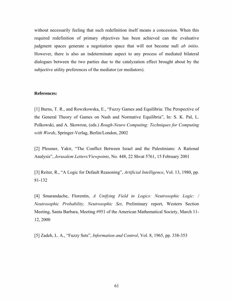
61

without necessarily feeling that such redefinition itself means a concession. When this

required redefinition of primary objectives has been achieved can the evaluative

judgment spaces generate a negotiation space that will not become null ab initio.

However, there is also an indeterminate aspect to any process of mediated bilateral

dialogues between the two parties due to the catalyzation effect brought about by the

subjective utility preferences of the mediator (or mediators).

References:

[1] Burns, T. R., and Rowzkowska, E., “Fuzzy Games and Equilibria: The Perspective of

the General Theory of Games on Nash and Normative Equilibria”, In: S. K. Pal, L.

Polkowski, and A. Skowron, (eds.) Rough-Neuro Computing: Techniques for Computing

with Words, Springer-Verlag, Berlin/London, 2002

[2] Plessner, Yakir, “The Conflict Between Israel and the Palestinians: A Rational

Analysis”, Jerusalem Letters/Viewpoints, No. 448, 22 Shvat 5761, 15 February 2001

[3] Reiter, R., “A Logic for Default Reasoning”, Artificial Intelligence, Vol. 13, 1980, pp.

81-132

[4] Smarandache, Florentin, A Unifying Field in Logics: Neutrosophic Logic: /

Neutrosophic Probability, Neutrosophic Set, Preliminary report, Western Section

Meeting, Santa Barbara, Meeting #951 of the American Mathematical Society, March 11-

12, 2000

[5] Zadeh, L. A., “Fuzzy Sets”, Information and Control, Vol. 8, 1965, pp. 338-353

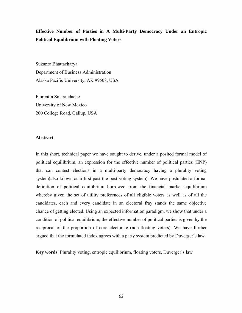
62

Effective Number of Parties in A Multi-Party Democracy Under an Entropic

Political Equilibrium with Floating Voters

Sukanto Bhattacharya

Department of Business Administration

Alaska Pacific University, AK 99508, USA

Florentin Smarandache

University of New Mexico

200 College Road, Gallup, USA

Abstract

In this short, technical paper we have sought to derive, under a posited formal model of

political equilibrium, an expression for the effective number of political parties (ENP)

that can contest elections in a multi-party democracy having a plurality voting

system(also known as a first-past-the-post voting system). We have postulated a formal

definition of political equilibrium borrowed from the financial market equilibrium

whereby given the set of utility preferences of all eligible voters as well as of all the

candidates, each and every candidate in an electoral fray stands the same objective

chance of getting elected. Using an expected information paradigm, we show that under a

condition of political equilibrium, the effective number of political parties is given by the

reciprocal of the proportion of core electorate (non-floating voters). We have further

argued that the formulated index agrees with a party system predicted by Duverger’s law.

Key words: Plurality voting, entropic equilibrium, floating voters, Duverger’s law

63

Introduction

Plurality voting systems are currently used in over forty countries worldwide which

include some of the largest democracies like USA, Canada, India and UK. Under the

basic plurality voting system, a country is divided into territorial single-member

constituencies; voters within each constituency cast a single ballot (typically marked by a

X) for one candidate; and the candidate with the largest share of votes in each seat is

returned to office; and the political party (or a confederation of ideologically similar

political parties) with an overall majority of seats forms the government. The

fundamental feature of the plurality voting system is that single-member constituencies

are based on the size of the electorate. For example, the US is divided into 435

Congressional districts each including roughly equal populations with one House

representative per district. Boundaries of constituencies are reviewed at periodic intervals

based on the national census to maintain the electorate balance. However the number of

voters per constituency varies dramatically across countries e.g. India has 545

representatives for a population of over nine hundred million, so each member of the Lok

Sabha (House of the People) serves nearly two million people, while in contrast Ireland

has 166 members in the Dial for a population slightly more than three-and-half million or

approximately one seat for a little over twenty thousand people.

Under the first-past-the-post voting system candidates only need a simple plurality i.e. at

least one more vote than their closest rival to get elected. Hence in three-way electoral

contests, the winning candidate can theoretically have less than fifty percent of votes cast

in his or her favor e.g. if the vote shares are 35%, 34% and 31%, the candidate with a

35% vote share will get elected. Therefore, although two-thirds of voters support other

candidates, the candidate with a simple plurality of votes wins the contest (Norris, 1997).

We define political equilibrium as a condition in which the choices of voters and political

parties are all compatible and in which no one group can improve its position by making

a different choice. In essence therefore, political equilibrium may be said to exist when,

given the set of utility preferences of all eligible voters as well as of all the candidates,

64

each and every candidate in an electoral fray stands the same chance of getting elected.

This definition is adequately broad to cover more specific conditional equilibrium models

and is based on the principle of efficiency as applied to financial markets. Daniel Sutter

(2002) defines political equilibrium as “a balance between demands by citizens on the

political system and candidates compete for office”. Therefore, translated to a multi-party

democracy having a plurality voting system, political equilibrium can be thought to imply

a state where perfect balance of power exists between all contesting parties.

Methodologically, we build our formal equilibrium model using an expected information

approach used in a generalized financial market equilibrium model (Bhattacharya, 2001).

Computing an effective number of political parties

Is there a unique optimum for the number of political parties that have to compete in

order to ensure a political equilibrium? If there indeed is such an optimal number then

this number necessarily has to be central to any theoretical formalization of political

equilibrium as we have defined. Rae (1967) advanced the first formal expression for

political fractionalization in a multi-party democracy as follows:

Fs = 1–3(si)2

Here Fs is known as Rae’s index of political fractionalization and si is the proportion of

seats of the ith political party in the Parliament. Conceptually, Rae’s fractionalization

index is adapted from the Herfindahl-Hirschman market power concentration index. F is

0 for a single-party system and F tends to 0.50 for a two-party system in equilibrium i.e.

when both parties command same proportion of seats in the Parliament. Of course F

asymptotically approaches unity as the party system becomes more and more

fractionalized. Of course, one may adapt Rae’s fractionalization index in terms of the

proportion of votes secured in an election instead of seats in Parliament. In that case

Rae’s index of fractionalization may be represented as follows:

65

Fv = 1–3(vi)2

Dumont and Caulier (2003) have recognized two major drawbacks of Rae’s index.

Firstly, the index is not linear for parties that are tied in strength; measured either as

proportion of seats or proportion of votes. A two-party system in equilibrium produces an

F of 0.50 whereas a four-party system in equilibrium produces 0.75 and a five-party

system in equilibrium will have an F of 0.80. Dumont and Caulier (2003) point out that

this feature makes the F untenable as an index as the operationalized measure and the

phenomenon it measures follow different progression paths. Secondly, Rae’s index is,

like most other normalized indices of social phenomena, extremely difficult to interpret

in objective terms as a unique variable characterizing a party system. The effective

number of parties (ENP) measure formulated by Laakso and Taagepera (1979) by

improving on Rae’s index is now commonly regarded as the classical numerical measure

for the comparative analysis of party systems. This ENP formula takes both the number

of parties and their relative weights into account when computing a unique variable

characterizing a party system thereby making objective interpretation a lot easier as

compared to Rae’s fractionalization index. The ENP formula is simply stated as the

reciprocal of the complement of Rae’s fractionalization index i.e.

ENPs= (1 – Fs)-1 and ENPv = (1 – Fv)-1

In equilibrium, all political parties will command the same strength measured either as

proportion of seats or votes and ENP will exactly equal the number of parties in fray.

Taagepera and Shugart (1989) have argued that the ENP has become a widely-used index

because it “usually tends to agree with our average intuition about the number of serious

parties”. However Molinar (1991) and Dunleavy and Boucek (2003) have argued that this

index produces counter-intuitive and counter-empirical results under a number of

circumstances. Taagepera (1999) himself suggested that in cases where one party clearly

dominates the political system (commanding more than 50% of the seats), an additional

index called the LC (Largest Component) index should be used in conjunction with ENP.

The LC is simply the reciprocal of the share of the largest party. When LC is greater than

66

2 for any party, that party clearly dominates the political system which would however be

classified as a multi-party system if only the ENP was the sole classification criterion.

Dunleavy and Boucek (2003) have advocated the averaging of ENP index with the LC

index to yield a unique classification criterion. Dumont and Caulier (2003) advanced the

effective number of relevant parties measure (ENRP) as an improvement over the ENP in

a way that their measure yields a unique classification criterion that roughly corresponds

to the ENP measure when there are more than two parties that can be considered as major

contenders for victory in an electoral contest and collapses to unity if there are only one

or two parties that can be seriously considered as a potential winner.

Irrespective of which variant of the ENP index we consider, it is obvious that an intuitive

paradigm formalizing political equilibrium in a multi-party democracy having a plurality

voting system may be constructed if it can be shown that in equilibrium, all parties in fray

are indeed expected to command an equal strength measured either in terms of seats or

votes. But such formalization would be considered somewhat limited if it did not take

into account the impact of floating voters on electoral outcomes. These are the

quintessential fence-sitters who waver between parties during the course of a Parliament,

or who don’t make up their minds until very close to the election (or even until actually

putting their stamps on the ballot paper). The impact of floating voters on electoral

outcome is all the more an important issue for large-sized electorates as is the case for

very populous countries like India. But none of the ENP indices consider floating voters.

Effective number of political parties with floating voters in entropic equilibrium

Considering a finite fraction of floating voters in any electorate, we may define the

following relationship as the (conservative) expected vote share of the ith political party:

E(Vi) = [E(Si)](1 –λi)

Here E(Si) is the ith candidate’s expected vote share as a proportion of the total electorate

size and λi is the fraction of the ith candidate’s vote share that is deemed to come from

67

floating voters. This is the fraction of electorate which is generally supportive of the ith

candidate but this support may or may not be translated into actual votes on the day of the

election. Thus E(Si) is the expected proportion of votes to be cast in the ith candidate’s

favor accepting the existence of floating voters in the electorate. Therefore we may write:

3i E(Vi) = 3i [E(Si)](1 –λi)

Let us denote 3i E(Vi) as E(V) and 3i E(Si) as E(S). Therefore, re-arranging (5) we get:

3i [E(Si)] λi = E(S) – E(V)

In mathematical information theory, entropy or expected information from an event is

measured using a logarithmic function borrowed from classical thermodynamics. There

are two possible mutually exclusive and exhaustive outcomes for any individual event –

either the event occurs or the event does not occur. If there are m candidates in an

electoral fray the two events associated with each candidate in fray is that either the

particular candidate wins the election or he/she does not win. If pi is the probability of the

ith candidate winning the election, then the expected information content of a message

that conveys the outcome of an election with i = 1, 2, …, m candidates is obtained by the

classical entropy function as formulated by Shannon (1948) as follows:

ψ(p) = (–C′)3i(pi)log2(pi)

Here C′ is a positive scale factor (a negentropic counterpart of the Boltzmann constant in

thermodynamic entropy). Under an m-party political equilibrium, the long run core (non-

floating) vote shares of the i = 1, 2, …, m candidates in electoral fray may be considered

as equivalent to their long run winning probabilities. Thus ψ(p) is re-writable as follows:

ψ(1 –λ) = (–C′)3i(1 – λi)log2(1 – λi)

68

Proposition: If ψ(1 – λ) is the expected information from the knowledge of an electoral

outcome given the proportion of non-floating voters (1 –λi) in the vote share of the ith

candidate, then the effective number of parties under entropic equilibrium is given as:

ENP(λ) = (1 – λ*)–1; where λ* = 1 –E(V)/E(S)

Proof: Incorporating the Lagrangian multiplier L the objective function can be written as:

Z (1 – λi, L) = (–C′) 3i(1 – λi) log2 (1 – λi) + L{1 –3i(1 – λi)}

Taking partial derivative of Z with respect to (1 –λi) and setting equal to zero as per the

necessary condition of maximization, the following stationary condition is obtained:

∂Z/∂(1 – λi) = (–C′){log2(1 – λi) + 1} –L = 0

Therefore at the point of maximum entropy one gets log2(1 – λi) = – (L/C′+ 1) i.e. (1 λi)

becomes a constant value independent of i for all i = 1, 2, …, m candidates in the

electoral contest. Since necessarily the 1 – λi values must sum to unity, it implies that at

the point of maximum entropy we must have p1 = p2 =… = pm = (1 – λ*) = 1/m.

Therefore m ≡ ENP(λ) = (1 – λ*)–1

Simplifying the expression for 3i[E(Si)]λi = E(S) – E(V) under equilibrium we may

write:

λ*E(S) = E(S) – E(V) i.e. λ* = 1 –E(V)/E(S) Q.E.D.

λ* is simply the total percentage of floating voters under an entropic political

equilibrium1. Thus ENP(λ) is formally obtained (as expected intuitively) as the reciprocal

of the equilibrium percentage of non-floating voters in the electorate. The higher the

proportion of floating voters within the electorate, the higher is the value of ENP(λ). The

69

intuitive reasoning is obvious – with a large number of floating votes to go around, more

candidates could stay in the electoral fray than there would be if the electorate consisted

of only a very small percentage of floating voters. When λ = 50%, ENP(λ) = 2. If λ goes

up to 75%, ENP(λ) will go up to 4 i.e. with 25% more floating voters within the

electorate, 2 more candidates can stay in electoral fray feeding off the floating votes.

Thus ENP(λ) (the formula for which is structurally quite similar to Laakso and

Taagepera’s ENP index) is a generalized measure of ENP based on the entropic

formalization of political equilibrium accepting the very real existence of floating voters.

Entropic political equilibrium and Duverger’s law

Duverger (1951) stated that the electoral contest in a single-seat electoral constituency

following a plurality voting system tends to converge to a two-party system. Duverger’s

law basically stems from the premise of strategic voting. Palfrey (1989) has showed that

in large electorates, equilibrium voting behavior implies that a voter will always vote for

the most preferred candidate of the two frontrunners. For a given electorate of size n,

Palfrey’s model is stated in terms of the following inequality:

uk > uj [(3i≠j(pnij/pn

kl) / (3h≠k(pnkh/pn

kl)] + 3i≠j,k ui [{(pnki– pn

ij)/pnkl}/3h≠k(pn

kh/pnkl)]

In this model, uk denotes the voter’s utility of his/her first choice among the two

frontrunners and ul denotes the voter’s utility for his/her second choice among the

frontrunners so that uk > ul. Also j is any other candidate from among the i = 1, 2, …, m

candidates. The notation pnij stands for the probability that the candidate i and candidate j

are tied for the most votes and the interpretation is similar for notations pnkh and pnkl. In

the limiting case, the likelihood ratio pnkh/pnkl tends to zero for all ij ≠ kl. Thus the right-

hand side of the inequality converges to ul irrespective of j; thereby mathematically

establishing Duverger’s law. Apart from Palfrey’s theoretical formalization, Cox and

Amorem Neto (1997) and Benoit (1998) and Schneider (2004) have provided empirical

evidence generally supportive of Duverger’s law.

70

It therefore seems rather appropriate that an intuitive model of political equilibrium in a

multi-party democracy that follows a plurality voting system should at least take

Duverger’s law into consideration if not actually have it embedded in some form within

its formal structure. This is true for our entropic model, because as m increases (1 –λ*) = 1/m becomes smaller and smaller, thereby implying that for multi-party democracies that

follow a plurality voting system, the political equilibrium most likely to prevail in the

long run will tend to occur at the highest possible value of (1 –λ*) = 50%. In other

words, although some relatively new democracies may start off with a number of political

parties contesting elections and a very large percentage of floating voters in the

electorate, the likelihood is very low that a very high proportion (exceeding 50%) of the

electorate will be composed of floating voters in the long run which implies that in the

long run, “mature” multi-party democracies having plurality voting systems will tend to

have only two parties as serious contenders for victory in an election; corresponding to a

two-party system as stated by Duverger’s law.

Conclusion

We have proposed and mathematically derived a formula for the effective number of

political parties that can be in electoral fray under a condition of political equilibrium in a

multi-party democracy following a plurality voting system. We have posited the expected

information approach to formalize the concept of political equilibrium in a parliamentary

democracy. Our advocated model aims to improve upon existing ENP indices by

incorporating the very realistic consideration of the impact of floating voters on elections.

Of course, ours has been an entirely theoretical exercise and a potentially rewarding

direction of future research would be to empirically investigate the veracity of ENP(λ)

possibly in conjunction with a suitable classification model to distinguish floating voters.

71

References:

[1] Benoit, K. (1998)‘The Number of Parties: New Evidence from Local Elections’.

1998 Annual Meeting of the American Political Science Association, Boston Marriott

Copley Place and Sheraton Boston Hotel and Towers, September 3-6.

[2] Bhattacharya, S. (2001)‘Mathematical modeling of a generalized securities market as

a binary, stochastic system’. Journal of Statistics and Management Systems 4 (2): 137-45.

[3] Cox, G. W. and O. Amorem Neto. (1997)‘Electoral Institutions, Cleavage Structures

and the Number of Parties’. American Journal of Political Science 41: 149-74

[4] Dumont P. and J-F. Caulier. (2003)‘The Effective Number of Relevant Parties: How

Voting Power Improves Laakso-Taagepera’s Index’. Europlace Institute of Finance

working papers: http://www.institut-europlace.com/mapping/ief.phtml?m=14&r=919

(accessed on 10th October 2005).

[5] Dunleavy, P. and F. Boucek. (2003) ‘Constructing the Number of Parties’, Party

Politics 9(3): 291 – 315.

[6] Duverger, M. (1954) Political Parties: Their Organization and Activity in the Modern

State. London: Methuen; New York: John Wiley & Sons.

[7] Gabay, N. (1999) ‘Decoding 'Floating Votes' in Israeli Direct Elections: Allocation

Model based on Discriminant Analysis Technique’. Israeli Sociology A(2): 295 – 318.

[8] Laakso, M. and R. Taagepera. (1979) ‘Effective Number of Parties: A Measure with

Application to West Europe’. Comparative Political Studies 12: 3 – 27.

[9] Molinar, J. (1991)‘Counting the Number of Parties: An Alternative Index’. American

72

Political Science Review 85: 1383 – 91.

[10] Norris, P. (1997)‘Choosing Electoral Systems: Proportional, Majoritarian and Mixed

Systems’. International Political Science Review 18 (July): 297-312.

[11] Palfrey, T. R. (1989)‘A Mathematical Proof of Duverger’s Law’ in P. C. Ordeshook

(ed) Models of Strategic Choice in Politics, Ann Arbor: University of Mich. Press: 69 –

92.

[12] Rae, D. (1967) The Political Consequences of Electoral Laws. New Haven: Yale

University Press.

[13] Schneider, G. (2004) ‘Falling Apart or Flocking Together? Left-Right Polarization

in the OECD since World War II’. 2004 Workshop of the Polarization and Conflict

Network, Barcelona, December 10-12.

[14] Shannon, C. E. (1948) ‘A mathematical theory of communication’. Bell System

Technical Journal, 27(July): 379 - 423.

[15] Sutter, D. (2002) ‘The Democratic Efficiency Debate and Definitions of Political

Equilibrium’. The Review of Austrian Economics 15 (3): 199–209.

[16] Taagepera, R and M. S. Shugart. (1989) Seats and Votes: The Effects and

Determinants of Electoral Systems. New Haven: Yale University Press.

73

Notion of Neutrosophic Risk and Financial Markets Prediction

Dr. Sukanto Bhattacharya

Program Director - MBA Global Finance

Business Administration Department

Alaska Pacific University

4101 University Drive

Anchorage, AK 99508, USA

Abstract

In this paper we present an application of the neutrosophic logic in the prediction of the

financial markets.

1. Introduction The efficient market hypothesis based primarily on the statistical principle of Bayesian

inference has been proved to be only a special-case scenario. The generalized financial

market, modeled as a binary, stochastic system capable of attaining one of two possible

states (High → 1, Low → 0) with finite probabilities, is shown to reach efficient

equilibrium with p . M = p if and only if the transition probability matrix M2x2 obeys the

additionally imposed condition {m11 = m22, m12 = m21}, where mij is an element of M

(Bhattacharya, 2001). [1]

Efficient equilibrium is defined as the stationery condition p = [0.50, 0.50] i.e. the state

in t + 1 is equi-probable between the two possible states given the market vector in time t.

However, if this restriction {m11 = m22, m12 = m21} is removed, we get inefficient

equilibrium ρ = [m21/(1-v), m12/(1-v)], where v = m11 – m21 may be derived as the

eigenvalue of M and ρ is a generalized version of p whereby the elements of the market

vector are no longer restricted to their efficient equilibrium values. Though this proves

74

that the generalized financial market cannot possibly get reduced to pure random walk if

we do away with the assumption of normality, it does not necessarily rule out the

possibility of mean reversion as M itself undergoes transition over time implying a

probable re-establishment of the condition {m11 = m22, m12 = m21} at some point of time

in the foreseeable future. The temporal drift rate may be viewed as the mean reversion

parameter k such that kjMt → Mt+j. In particular, the options market demonstrates a

rather perplexing departure from efficiency. In a Black-Scholes type world, if stock price

volatility is known a priori, the option prices are completely determined and any

deviations are quickly arbitraged away.

Therefore, statistically significant mispricings in the options market are somewhat

unique as the only non-deterministic variable in option pricing theory is volatility.

Moreover, given the knowledge of implied volatility on the short-term options, the

miscalibration in implied volatility on the longer term options seem odd as the parameters

of the process driving volatility over time can simply be estimated by an AR1 model

(Stein, 1993). [2]

Clearly, the process is not quite as straightforward as a simple parameter estimation

routine from an autoregressive process. Something does seem to affect the market

players’ collective pricing of longer term options, which clearly overshadows the

straightforward considerations of implied volatility on the short-term options. One clear

reason for inefficiencies to exist is through overreaction of the market players to new

information. Some inefficiency however may also be attributed to purely random white

noise unrelated to any coherent market information. If the process driving volatility is

indeed mean reverting then a low implied volatility on an option with a shorter time to

expiration will be indicative of a higher implied volatility on an option with a longer time

to expiration. Again, a high implied volatility on an option with a shorter time to

expiration will be indicative of a lower implied volatility on an option with a longer time

to expiration. However statistical evidence often contradicts this rational expectations

hypothesis for the implied volatility term structure.

Denoted by σ’t (t), (where the symbol ’ indicates first derivative) the implied volatility

at time t of an option expiring at time T is given in a Black-Scholes type world as

follows:

75

σ’t (t) = j=0∫T [{σM + kj (σt - σM)}/T] dj

σ’t (t) = σM + (kT – 1)(σt - σM)/(T ln k) (1)

Here σt evolves according to a continuous-time, first-order Wiener process as follows:

dσt = - β0 (σt - σM) dt + β1σt ε√dt (2)

β0 = - ln k, where k is the mean reversion parameter. Viewing this as a mean reverting

AR1 process yields the expectation at time t, Et (σt+j), of the instantaneous volatility at

time t+j, in the required form as it appears under the integral sign in equation (1).

This theorizes that volatility is rationally expected to gravitate geometrically back

towards its long-term mean level of σM. That is, when instantaneous volatility is above its

mean level (σt > σM), the implied volatility on an option should be decreasing as t → T.

Again, when instantaneous volatility is below the long-term mean, it should be rationally

expected to be increasing as t → T. That this theorization does not satisfactorily reflect

reality is attributable to some kind combined effect of overreaction of the market players

to excursions in implied volatility of short-term options and their corresponding

underreaction to the historical propensity of these excursions to be rather short-lived.

2. A Cognitive Dissonance Model of Behavioral Market Dynamics

Whenever a group of people starts acting in unison guided by their hearts rather than

their heads, two things are seen to happen. Their individual suggestibilities decrease

rapidly while the suggestibility of the group as a whole increases even more rapidly. The

‘leader’, who may be no more than just the most vociferous agitator, then primarily

shapes the groupthink. He ultimately becomes the focus of the group opinion. In any

financial market, it is the gurus and the experts who often play this role. The crowd hangs

on their every word and makes them the uncontested Oracles of the marketplace.

76

If figures and formulae continue to speak against the prevailing groupthink, this could

result into a mass cognitive dissonance calling for reinforcing self-rationalizations to be

strenuously developed to suppress this dissonance. As individual suggestibilities are at a

lower level compared to the group suggestibility, these self-rationalizations can actually

further fuel the prevailing groupthink. This groupthink can even crystallize into

something stronger if there is also a simultaneous vigilance depression effect caused by a

tendency to filter out the dissonance-causing information. The non-linear feedback

process keeps blowing up the bubble until a critical point is reached and the bubble bursts

ending the prevailing groupthink with a recalibration of the position by the experts.

Our proposed model has two distinct components – a linear feedback process containing

no looping and a non-linear feedback process fuelled by an unstable rationalization loop.

It is due to this loop that perceived true value of an option might be pushed away from its

theoretical true value. The market price of an option will follow its perceived true value

rather than its theoretical true value and hence the inefficiencies arise. This does not

mean that the market as a whole has to be inefficient – the market can very well be close

to strong efficiency! Only it is the perceived true value that determines the actual price-

path meaning that all market information (as well as some of the random white noise)

gets automatically anchored to this perceived true value. This would also explain why

excursions in short-term implied volatilities tend to dominate the historical considerations

of mean reversion – the perceived term structure simply becomes anchored to the

prevailing groupthink about the nature of the implied volatility.

Our conceptual model is based on two primary assumptions:

The unstable rationalization loop comes into effect if and only if the group is a

reasonably well-bonded one i.e. if the initial group suggestibility has already attained a

certain minimum level as, for example, in cases of strong cartel formations and;

The unstable rationalization loop stays in force till some critical point in time t* is

reached in the life of the option. Obviously t* will tend to be quite close to T – the time

of expiration. At that critical point any further divergence becomes unsustainable due to

77

the extreme pressure exerted by real economic forces ‘gone out of sync’ and the gap

between perceived and theoretical true values close very rapidly.

2.1. The Classical Cognitive Dissonance Paradigm

Since Leon Festinger presented it well over four decades ago, cognitive dissonance

theory has continued to generate a lot of interest as well as controversy. [3] [4] This was

mainly due to the fact that the theory was originally stated in very generalized, abstract

terms. As a consequence, it presented possible areas of application covering a number of

psychological issues involving the interaction of cognitive, motivational, and emotional

factors. Festinger’s dissonance theory began by postulating that pairs of cognitions

(elements of knowledge), given that they are relevant to one another, can either be in

agreement with each other or otherwise. If they are in agreement they are said to be

consonant, otherwise they are termed dissonant. The mental condition that forms out of a

pair of dissonant cognitions is what Festinger calls cognitive dissonance.

The existence of dissonance, being psychologically uncomfortable, motivates the person

to reduce the dissonance by a process of filtering out information that are likely to

increase the dissonance. The greater the degree of the dissonance, the greater is the

pressure to reduce dissonance and change a particular cognition. The likelihood that a

particular cognition will change is determined by the resistance to change of the

cognition. Again, resistance to change is based on the responsiveness of the cognition to

reality and on the extent to which the particular cognition is in line with various other

cognitions. Resistance to change of cognition depends on the extent of loss or suffering

that must be endured and the satisfaction or pleasure obtained from the behavior. [5] [6]

[7] [8] [9] [10] [11] [12]

We propose the conjecture that cognitive dissonance is one possible (indeed highly

likely) critical behavioral trigger [13] that sets off the rationalization loop and

subsequently feeds it.

78

2.2 Non-linear Feedback Statistics Generating a Rationalization Loop

In a linear autoregressive model of order R, a time series yn is modeled as a linear

combination of N earlier values in the time series, with an added correction term xn:

yn = xn - Σaj yn-j (3)

The autoregressive coefficients aj (j = 1, ... N) are fitted by minimizing the mean-squared

difference between the modeled time series yn and the observed time series yn. The

minimization process results in a system of linear equations for the coefficients an, known

as the Yule-Walker equations. Conceptually, the time series yn is considered to be the

output of a discrete linear feedback circuit driven by a noise xn, in which delay loops of

lag j have feedback strength aj. For Gaussian signals, an autoregressive model often

provides a concise description of the time series yn, and calculation of the coefficients aj

provides an indirect but highly efficient method of spectral estimation. In a full nonlinear

autoregressive model, quadratic (or higher-order) terms are added to the linear

autoregressive model. A constant term is also added, to counteract any net offset due to

the quadratic terms:

yn = xn - a0 - Σaj yn-j - Σbj, k yn-jyn-k (4)

The autoregressive coefficients aj (j = 0, ... N) and bj, k (j, k = 1, ... N) are fit by

minimizing the mean-squared difference between the modeled time series yn and the

observed time series yn*. The minimization process also results in a system of linear

equations, which are generalizations of the Yule-Walker equations for the linear

autoregressive model.

Conceptually, the time series yn is considered to be the output of a circuit with nonlinear

feedback, driven by a noise xn. In principle, the coefficients bj, k describes dynamical

features that are not evident in the power spectrum or related measures. Although the

equations for the autoregressive coefficients aj and bj, k are linear, the estimates of these

parameters are often unstable, essentially because a large number of them must be

79

estimated often resulting in significant estimation errors. This means that all linear

predictive systems tend to break down once a rationalization loop has been generated. As

parameters of the volatility driving process, which are used to extricate the implied

volatility on the longer term options from the implied volatility on the short-term ones,

are estimated by an AR1 model, which belongs to the class of regression models

collectively referred to as the GLIM (General Linear Model), the parameter estimates go

‘out of sync’ with those predicted by a theoretical pricing model.

Unfortunately, there is no straightforward method to distinguish linear time series

models (H0) from non-linear alternatives (HA). The approach generally taken is to test the

H0 of linearity against a pre-chosen particular non-linear HA. Using the classical theory of

statistical hypothesis testing, several test statistics have been developed for this purpose.

They can be classified as Lagrange Multiplier (LM) tests, likelihood ratio (LR) tests and

Wald (W) tests. The LR test requires estimation of the model parameters both under H0

and HA, whereas the LM test requires estimation only under H0. Hence in case of a

complicated, non-linear HA containing many more parameters as compared to the model

under H0, the LM test is far more convenient to use. On the other hand, the LM test is

designed to reveal specific types of non-linearities. The test may also have some power

against inappropriate alternatives. However, there may at the same time exist alternative

non-linear models against which an LM test is not powerful. Thus rejecting H0 on the

basis of such a test does not permit robust conclusions about the nature of the non-

linearity. One possible solution to this problem is using a W test which estimates the

model parameters under a well-specified non-linear HA [14].

3. The Zadeh argument revisited In the face of non-linear feedback processes generated by dissonant information

sources, even mathematically sound rule-based reasoning schemes often tend to break

down. As a pertinent illustration, we take Zadeh’s argument against the well-known

Dempster’s rule [15] [16]. Let Θ = {θ1, θ2 … θn} stand for a set of n mutually exhaustive,

80

elementary events that cannot be precisely defined and classified making it impossible to

construct a larger set Θref of disjoint elementary hypotheses.

The assumption of exhaustiveness is not a strong one because whenever θj, j = 1, 2 … n

does not constitute an exhaustive set of elementary events, one can always add an extra

element θ0 such that θj, j = 0, 1 … n describes an exhaustive set. Then, if Θ is considered

to be a general frame of discernment of the problem under consideration, a map m (.): DΘ

→ [0, 1] may be defined associated with a given body of evidence B that can support

paradoxical information as follows:

m (φ) = 0 (5)

ΣA∈DΘ m (A) = 1 (6)

Then m (A) is called A’s basic probability number. In line with the Dempster-Shafer

Theory, the belief and plausibility functions are defined as follows:

Bel (A) = ΣB∈DΘ

, B⊆A m (B) (7)

Pl (A) = ΣB∈DΘ

, B∩A ≠ φ m (B) (8)

Now let Bel1 (.) and Bel2 (.) be two belief functions over the same frame of discernment

Θ and their corresponding information granules m1 (.) and m2 (.). Then the combined

global belief function is obtained as Bel1 (.) = Bel1 (.) ⊕ Bel2 (.) by combining the

information granules m1 (.) and m2 (.) as follows for m (φ) = 0 and for any C ≠ 0 and C ⊆

Θ;

[m1 ⊕ m2] (C) = [ΣA∩B=C m1 (A) m2 (B)] / [1 - ΣA∩B = φ m1 (A) m2 (B)]

(9)

The summation notation ΣA∩B=C is necessarily interpreted as the sum over all A, B ⊆ Θ

such that A ∩ B = C. The orthogonal sum m (.) is considered a basic probability

assignment if and only if the denominator in equation (5) is non-zero. Otherwise the

81

orthogonal sum m (.) does not exist and the bodies of evidences B1 and B2 are said to be

in full contradiction.

Such a case can arise when there exists A ⊂ Θ such that Bel1 (A) =1 and Bel2 (Ac) = 1 –

a problem associated with optimal Bayesian information fusion rule (Dezert, 2001).

Extending Zadeh’s argument to option market anomalies, if we now assume that under

conditions of asymmetric market information, two market players with homogeneous

expectations view implied volatility on the long-term options. One of them sees it as

either arising out of (A) current excursion in implied volatility on short-term options with

probability 0.99 or out of (C) random white noise with probability of 0.01. The other sees

it as either arising out of (B) historical pattern of implied volatility on short-run options

with probability 0.99 or out of (C) random white noise with probability of 0.01.

Using Dempster’s rule of combination, the unexpected final conclusion boils down to the

expression m (C) = [m1 ⊕ m2] (C) = 0.0001/(1 – 0.0099 – 0.0099 – 0.9801) = 1 i.e. the

determinant of implied volatility on long-run options is random white noise with absolute

certainty!

To deal with this information fusion problem a new combination rule has been proposed

under the name of Dezert-Smarandache combination rule of paradoxical sources of

evidence, which looks for the optimal combination i.e. the basic probability assignment

m (.) = m1 (.) ⊕ m2 (.) that maximizes the joint entropy of the two information sources

[17].

The Zadeh illustration originally sought to bring out the fallacy of automated reasoning

based on the Dempster’s rule and showed that some form of the degree of conflict

between the sources must be considered before applying the rule. However, in the context

of financial markets this assumes a great amount of practical significance in terms of how

it might explain some of the recurrent anomalies in rule-based information processing by

inter-related market players in the face of apparently conflicting knowledge sources. The

traditional conflict between the fundamental analysts and the technical analysts over the

credibility of their respective knowledge sources is of course all too well known!

82

4. Market Information Reconciliation Based on the Concept of Neutrosophic Risk

Neutrosophy is a new branch of philosophy that is concerned with neutralities and their

interaction with various ideational spectra. Let T, I, F be real subsets of the non-standard

interval ]-0, 1+[. If ε > 0 is an infinitesimal such that for all positive integers n and we

have |ε| < 1/n, then the non-standard finite numbers 1+ = 1+ε and 0- = 0-ε form the

boundaries of the non-standard interval ]-0, 1+[. Statically, T, I, F are subsets while

dynamically they may be viewed as set-valued vector functions. If a logical proposition is

said to be t% true in T, i% indeterminate in I and f% false in F then T, I, F are referred to

as the neutrosophic components. Neutrosophic probability is useful to events that are

shrouded in a veil of indeterminacy like the actual implied volatility of long-term options.

As this approach uses a subset-approximation for truth-values, indeterminacy and falsity-

values it provides a better approximation than classical probability to uncertain events.

The neutrosophic probability approach also makes a distinction between “relative sure

event”, event that is true only in certain world(s): NP (rse) = 1, and “absolute sure event”,

event that is true for all possible world(s): NP (ase) =1+. Similar relations can be drawn

for “relative impossible event” / “absolute impossible event” and “relative indeterminate

event” / “absolute indeterminate event”. In case where the truth- and falsity-components

are complimentary i.e. they sum up to unity, and there is no indeterminacy and one is

reduced to classical probability. Therefore, neutrosophic probability may be viewed as a

generalization of classical and imprecise probabilities. [18]

When a long-term option priced by the collective action of the market players is

observed to be deviating from the theoretical price, three possibilities must be considered:

(1) The theoretical price is obtained by an inadequate pricing model, which means that

the market price may well be the true price,

(2) An unstable rationalization loop has taken shape that has pushed the market price of

the option ‘out of sync’ with its true price, or

(3) The nature of the deviation is indeterminate and could be due to either (a) or (b) or a

super-position of both (a) and (b) and/or due to some random white noise.

However, it is to be noted that in none of these three possible cases are we referring to

the efficiency or otherwise of the market as a whole. The market can only be as efficient

83

as the information it gets to process. We term the systematic risk associated with the

efficient market as resolvable risk. Therefore, if the information about the true price of

the option is misleading (perhaps due to an inadequate pricing model), the market cannot

be expected to process it into something useful – after all, the markets can’t be expected

to pull jack-rabbits out of empty hats! The perceived risk resulting from the imprecision

associated with how human psycho-cognitive factors subjectively interpret information

and use the processed information in decision-making is what we term as irresolvable (or

neutrosophic) risk.

With T, I, F as the neutrosophic components, let us now define the following events:

H = {p: p is the true option price determined by the theoretical pricing model} and

M = {p: p is the true option price determined by the prevailing market price}

(10)

Then there is a t% chance that the event (H ∩ Mc) is true, or corollarily, the

corresponding complimentary event (Hc ∩ M) is untrue, there is a f% chance that the

event (Mc ∩ H) is untrue, or corollarily, the complimentary event (M ∩ Hc) is true and

there is a i% chance that neither (H ∩ Mc) nor (M ∩ Hc) is true/untrue; i.e. the

determinant of the true market price is indeterminate. This would fit in nicely with

possibility (c) enumerated above – that the nature of the deviation could be due to either

(a) or (b) or a super-position of both (a) and (b) and/or due to some random white noise.

Illustratively, a set of AR1 models used to extract the mean reversion parameter driving

the volatility process over time have coefficients of determination in the range say

between 50%-70%, then we can say that t varies in the set T (50% - 70%). If the

subjective probability assessments of well-informed market players about the weight of

the current excursions in implied volatility on short-term options lie in the range say

between 40%-60%, then f varies in the set F (40% - 60%). Then unexplained variation in

the temporal volatility driving process together with the subjective assessment by the

market players will make the event indeterminate by either 30% or 40%. Then the

84

neutrosophic probability of the true price of the option being determined by the

theoretical pricing model is NP (H ∩ Mc) = [(50 – 70), (40 – 60), {30, 40}].

5. Conclusion Finally, in terms of our behavioral conceptualization of the market anomaly primarily as

manifestation of mass cognitive dissonance, the joint neutrosophic probability NP (H ∩

Mc) will also be indicative of the extent to which an unstable rationalization loop has

formed out of such mass cognitive dissonance that is causing the market price to deviate

from the true price of the option. Obviously increasing strength of the non-linear

feedback process fuelling the rationalization loop will tend to increase this deviation. As

human psychology; and consequently a lot of subjectivity; is involved in the process of

determining what drives the market prices, neutrosophic reasoning will tend to reconcile

market information much more realistically than classical probability theory.

Neutrosophic reasoning approach will also be an improvement over rule-based reasoning

possibly avoiding pitfalls like that brought out by Zadeh’s argument. This has particularly

significant implications for the vast majority of market players who rely on signals

generated by some automated trading system following simple rule-based logic.

However, the fact that there is inherent subjectivity in processing the price information

coming out of financial markets, given that the way a particular piece of information is

subjectively interpreted by an individual investor may not be the globally correct

interpretation, there is always the matter of irresolvable risk that will tend to pre-dispose

the investor in favour of some safe investment alternative that offers some protection

against both resolvable as well as irresolvable risk. This highlights the rapidly increasing

importance and popularity of safe investment options that are based on some form of

portfolio insurance i.e. an investment mechanism where the investor has some kind of in-

built downside protection against adverse price movements resulting from erroneous

interpretation of market information e.g. constant proportion portfolio insurance (CPPI)

and its generalized form – options based portfolio insurance (OBPI). Such portfolio

insurance strategies offer protection against all possible downsides, whether resulting out

85

of resolvable or irresolvable risk, thereby making the investors feel confident about the

decisions they take.

References

[1] Bhattacharya, S., “Mathematical modelling of a generalized securities market as a

binary, stochastic system”, Journal of Statistics and Management Systems, July 2001,

pp137-145

[2] Stein, Jeremy, “Overreaction in the options markets”, in Advances in Behavioral

Finance, Richard H. Thaler, (Ed.), N.Y., Russell Sage Foundation, 1993, pp 341-355

[3] Festinger, L., A theory of cognitive dissonance, Evanston, IL: Row, Peterson, 1957

[4] Festinger, L., Carlsmith, J. M., “Cognitive consequences of forced compliance”,

Journal of Abnormal and Social Psychology, 58, 1959, pp203-210

[5] Aronson, E., “Dissonance theory: Progress and problems”, in R. P. Abelson, E.

Aronson, W. J. McGuire, T. M. Newcomb, M. J. Rosenberg, & P. H. Tannenbaum (Eds.),

Theories of cognitive consistency: A sourcebook, Chicago: Rand McNally, 1968, pp5-27

[6] Bem, D. J. “Self-perception: An alternative interpretation of cognitive dissonance

phenomena”, Psychological Review, 74, 1967, pp183-200

[7] Elliot, A. J., & Devine, P. G., “On the motivational nature of cognitive dissonance:

Dissonance as psychological discomfort”, Journal of Personality and Social Psychology,

67, 1994, pp382-394

[8] Gerard, H. B., “Choice difficulty, dissonance and the decision sequence”, Journal of

Personality, 35, 1967, pp91-108

[9] Scher, S. J., & Cooper, J. “Motivational basis of dissonance: The singular role of

behavioral consequences”, Journal of Personality and Social Psychology, 56, 1989, pp

899-906

[10] Shultz, T. R., & Lepper, M. R., “Cognitive dissonance reduction as constraint

satisfaction”, Psychological Review, 103, 1996, pp219-240

86

[11] Griffin, Em, A First Look at Communication Theory, McGraw-Hill, Inc., 1997

[12] Tedeschi, J. T., Schlenker, B. R., & Bonoma, T. V., “Cognitive dissonance: Private

ratiocination or public spectacle?”, American Psychologist, 26, 1971, pp. 680-695

[13] Allen, J. and Bhattacharya, S. “Critical Trigger Mechanism – a Modelling Paradigm

for Cognitive Science Application in the Design of Artificial Learning Systems”,

Smarandache Notions Journal, Vol. 13, 2002, pp. 43-47

[14] De Gooijer, J. G. and Kumar, K. “Some recent developments in non-linear time

series modeling, testing and forecasting”, International Journal of Forecasting 8, 1992,

pp. 135-156

[15] Zadeh, L. A., “The Concept of a Linguistic variable and its Application to

Approximate Reasoning I, II, III”, Information Sciences, Vol. 8, Vol. 9, 1975

[16] Zadeh, L. A., “A Theory of Approximate Reasoning”, Machine Intelligence, J.

Hayes, D. Michie and L. Mikulich (Eds.), Vol. 9, 1979, pp. 149-194

[17] Dezert, Jean, “Combination of paradoxical sources of information within the

Neutrosophic framework”, Proceedings of the First International Conference on

Neutrosophy, Neutrosophic Logic, Neutrosophic Set, Neutrosophic Probability and

Statistics, University of New Mexico, Gallup Campus, 1-3 December 2001, pp. 22-46

[18] Smarandache, Florentin, A Unifying Field in Logics: Neutrosophic Logic: /

Neutrosophic Probability, Neutrosophic Set, Preliminary report, Western Section

Meeting, Santa Barbara, Meeting #951 of the American Mathematical Society, March 11-

12, 2000

87

How Extreme Events Can Affect a Seemingly Stabilized Population: a Stochastic Rendition of Ricker’s Model S. Bhattacharya Department of Business Administration Alaska Pacific University, U.S.A. E-mail: sbhattacharya@alaskapacific.edu S. Malakar Department of Chemistry and Biochemistry University of Alaska, U.S.A. F. Smarandache Department of Mathematics University of New Mexico, U.S.A. Abstract Our paper computationally explores Ricker’s predator satiation model with the objective of studying how the extinction dynamics of an animal species having a two-stage life-cycle is affected by a sudden spike in mortality due to an extraneous extreme event. Our simulation model has been designed and implemented using sockeye salmon population data based on a stochastic version of Ricker’s model; with the shock size being reflected by a sudden reduction in the carrying capacity of the environment for this species. Our results show that even for a relatively marginal increase in the negative impact of an extreme event on the carrying capacity of the environment, a species with an otherwise stable population may be driven close to extinction. Key words: Ricker’s model, extinction dynamics, extreme event, Monte Carlo simulation Background and research objective PVA approaches do not normally consider the risk of catastrophic extreme events under the pretext that no population size can be large enough to guarantee survival of a species in the event of a large-scale natural catastrophe. [1] Nevertheless, it is only very intuitive that some species are more “delicate” than others; and although not presently under any clearly observed threat, could become threatened with extinction very quickly if an extreme event was to occur even on a low-to-moderate scale. The term “extreme event” is preferred to “catastrophe” because catastrophe usually implies a natural event whereas; quite clearly; the chance of man-caused extreme events poses a much greater threat at present to a number of animal species as compared to any large-scale natural catastrophe.

88

An animal has a two-stage life cycle when; in the first stage, newborns become immature youths and in the second stage; the immature youths become mature adults. Therefore, in terms of the stage-specific approach, if Yt denotes the number of immature young in stage t and At denotes the number of mature adults, then the number of adults in year t + 1 will be some proportion of the young, specifically those that survive to the next (reproductive) stage. Then the formal relationship between the number of mature adults in the next stage and the number of immature youths at present may be written as follows:

At + 1 = λYt Here λ is the survival probability, i.e. it is the probability of survival of a youth to maturity. The number of young next year will depend on the number of adults in t:

Yt + 1 = f (At) Here f describes the reproduction relation between mature adults and next year’s young. This is a straightforward system of simultaneous difference equations which may be analytically solved using a variation of the cobwebbing approach. [2] The solution process begins with an initial point (Y1, A1) and iteratively determines the next point (Y2, A2). If predator satiation is built into the process, then we simply end up with Ricker’s model:

Yt + 1 = αAte–At/K Here α is the maximum reproduction rate (for an initial small population) and K is the population size at which the reproduction rate is approximately half its maximum [3]. Putting β = 1/K we can re-write Ricker’s equation as follows:

Yt + 1 = αAte– βAt It has been shown that if (Y0, A0) lies within the first of three possible ranges, (Yn, An) approaches (0, 0) in successive years and the population becomes extinct. If (Y0, A0) lies within the third range then (Yn, An) equilibrate to a steady-state value of (Y*, A*). Populations that begin with (Y0, A0) within the second range oscillate between (Y*, 0) and (0, A*). Such alternating behavior indicates one of the year classes, or cohorts, become extinct while the other persists i.e. adult breeding stock appear only every other year. Thus the model reveals that three quite different results occur depending initially only on the starting sizes of the population and its distribution among the two stages. [4] We use the same basic model in our research but instead of analytically solving the system of difference equations, we use the same to simulate the population dynamics as a stochastic process implemented on an MS-Excel spreadsheet. Rather than using a closed-form equation like Ricker’s model to represent the functional relationship between Yt + 1 and At, we use a Monte Carlo method to simulate the stage-transition process within

89

Ricker’s framework; introducing a massive perturbation with a very small probability in order to emulate a catastrophic event.[5] Conceptual framework We have a formulated a stochastic population growth model with an inbuilt capacity to generate an extreme event based on a theoretical probability distribution. The non-stochastic part of the model corresponds to Ricker’s relationship between Yt + 1 and At. The stochastic part has to do with whether or not an extreme event occurs at a particular time point. The gamma distribution has been chosen to make the probability distribution for the extreme event a skewed one as it is likely to be in reality. Instead of analytically solving the system of simultaneous difference equations iteratively in some variation of the cobwebbing method, we have used them in a spreadsheet model to simulate the population growth over a span of ten time periods. We apply a computational methodology whereby the initial number of immature young is hypothesized to either attain the expected number predicted by Ricker’s model or drastically fall below that number at the end of every stage, depending on whether an extraneous extreme event does not occur or actually occurs. The mortalities as a result of an extreme event at any time point is expressed as a percentage of the pristine population size for a clearer comparative view. Model building Among various faunal species, the population dynamics of the sockeye salmon (oncorhynchus nerka) has been most extensively studied using Rickert’s model. Salmon are unique in that they breed in particular fresh water systems before they die. Their offspring migrates to the ocean and upon reproductive maturity, they are guided by a hitherto unaccounted instinctive drive to swim back to the very same fresh waters where they were born to spawn their own offspring and perish. Salmon populations thus are very sensitive to habitat changes and human activities that have a negative impact on riparian ecosystems that serve as breeding grounds for salmon can adversely affect the peculiar life-cycle of the salmon. Many of the ancient salmon runs (notably those in California river systems) have now gone extinct and it is our hypothesis that an even seemingly stabilized population can be rapidly driven to extinction due to the effect of an extraneous (quite possibly man-made) extreme event with the capacity to cause mass mortality. The following table shows the four-year averages of the sockeye salmon population in the Skeena river system in British Columbia in the first half of the twentieth century.

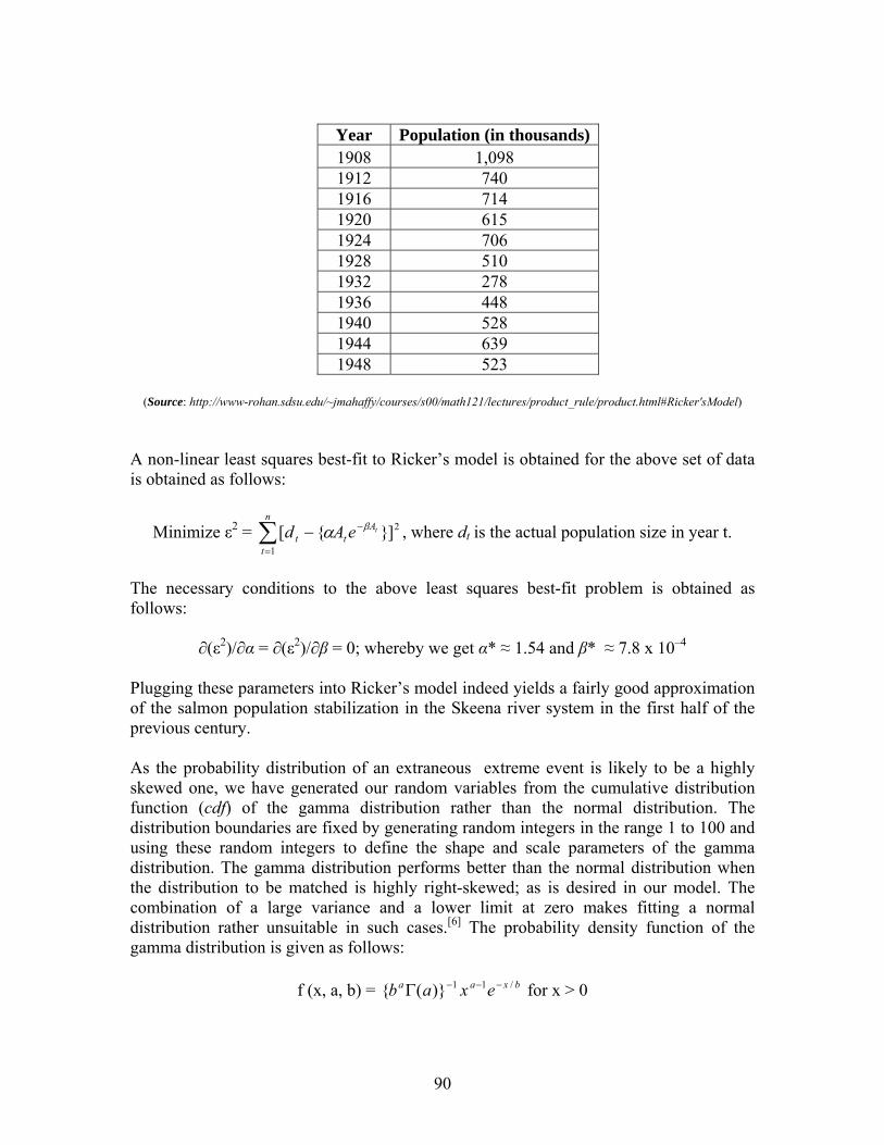
90

Year Population (in thousands)1908 1,098 1912 740 1916 714 1920 615 1924 706 1928 510 1932 278 1936 448 1940 528 1944 639 1948 523

(Source: http://www-rohan.sdsu.edu/~jmahaffy/courses/s00/math121/lectures/product_rule/product.html#Ricker'sModel)

A non-linear least squares best-fit to Ricker’s model is obtained for the above set of data is obtained as follows:

Minimize ε2 = 2

1

]}{[∑=

−−n

t

Att

teAd βα , where dt is the actual population size in year t.

The necessary conditions to the above least squares best-fit problem is obtained as follows:

∂(ε2)/∂α = ∂(ε2)/∂β = 0; whereby we get α* ≈ 1.54 and β* ≈ 7.8 x 10–4 Plugging these parameters into Ricker’s model indeed yields a fairly good approximation of the salmon population stabilization in the Skeena river system in the first half of the previous century. As the probability distribution of an extraneous extreme event is likely to be a highly skewed one, we have generated our random variables from the cumulative distribution function (cdf) of the gamma distribution rather than the normal distribution. The distribution boundaries are fixed by generating random integers in the range 1 to 100 and using these random integers to define the shape and scale parameters of the gamma distribution. The gamma distribution performs better than the normal distribution when the distribution to be matched is highly right-skewed; as is desired in our model. The combination of a large variance and a lower limit at zero makes fitting a normal distribution rather unsuitable in such cases.[6] The probability density function of the gamma distribution is given as follows:

f (x, a, b) = bxaa exab /11)}({ −−−Γ for x > 0

91

Here α > 0 is the shape parameter and β > 0 is the scale parameter of the gamma distribution. The cumulative distribution function may be expressed in terms of the incomplete gamma function as follows:

F (x, a, b) = ∫ Γ=x

abxaduuf0

)(/)/,()( γ

In our spreadsheet model, we have F (R, R/2, 2) as our cdf of the gamma distribution. Here R is an integer randomly sampled from the range 1 to 100. An interesting statistical result of having these values for x, α and β is that the cumulative gamma distribution value becomes equalized with the value [1 - χ2 (R)] having R degrees of freedom, thus allowing χ2 goodness-of-fit tests. [7] Our model is specifically designed to simulate the extinction dynamics of sockeye salmon population using a stochastic version of Ricker’s model; with the shock size being based on a sudden reduction in the parameter K i.e. the carrying capacity of the environment for this species. The model parameters are same as those of Ricker’s model i.e. α and β (which is the reciprocal of K). We have kept α constant at all times at 1.54, which was the least squares best-fit value obtained for that parameter. We have kept a β of 0.00078 (i.e. the best-fit value) when no extreme event occurs and have varied the β between 0.00195 and 0.0156 (i.e. between 2.5 times to 20 times the best-fit value) for cases where an extreme event occurred. We have a third parameter c which is basically a ‘switching constant’ that determines whether an extreme event occurs or not. The switch is turned on triggering an extreme event when a random draw from a cumulative gamma distribution yields a value less than or equal to c. Using F (R, R/2, 2) as our cdf of the gamma distribution where R is a randomly drawn integer in the range (1, 100) means that the cumulative gamma function will randomly select from the approximate interval 0.518 ~ 0.683. By fixing the value of c at 0.5189 in our model we have effectively reduced the probability of occurrence of an extreme event to a miniscule magnitude relative to that of an extreme event not occurring. We have used the sockeye salmon population data from the table presented earlier For each level of the β parameter, we simulated the system and observed the maximum possible number of mortalities from an extreme event at that level of β. The results are reported below.

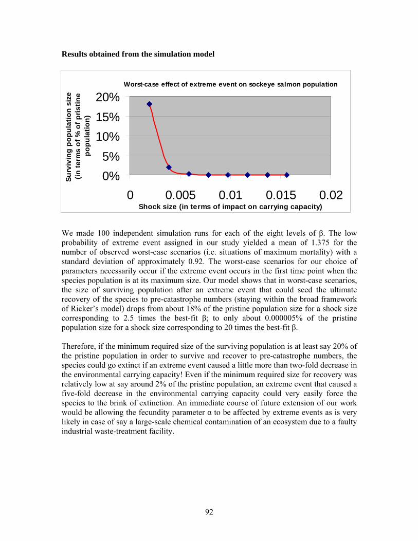
92

Results obtained from the simulation model We made 100 independent simulation runs for each of the eight levels of β. The low probability of extreme event assigned in our study yielded a mean of 1.375 for the number of observed worst-case scenarios (i.e. situations of maximum mortality) with a standard deviation of approximately 0.92. The worst-case scenarios for our choice of parameters necessarily occur if the extreme event occurs in the first time point when the species population is at its maximum size. Our model shows that in worst-case scenarios, the size of surviving population after an extreme event that could seed the ultimate recovery of the species to pre-catastrophe numbers (staying within the broad framework of Ricker’s model) drops from about 18% of the pristine population size for a shock size corresponding to 2.5 times the best-fit β; to only about 0.000005% of the pristine population size for a shock size corresponding to 20 times the best-fit β. Therefore, if the minimum required size of the surviving population is at least say 20% of the pristine population in order to survive and recover to pre-catastrophe numbers, the species could go extinct if an extreme event caused a little more than two-fold decrease in the environmental carrying capacity! Even if the minimum required size for recovery was relatively low at say around 2% of the pristine population, an extreme event that caused a five-fold decrease in the environmental carrying capacity could very easily force the species to the brink of extinction. An immediate course of future extension of our work would be allowing the fecundity parameter α to be affected by extreme events as is very likely in case of say a large-scale chemical contamination of an ecosystem due to a faulty industrial waste-treatment facility.

Worst-case effect of extreme event on sockeye salmon population

0%5%

10%15%20%

0 0.005 0.01 0.015 0.02Shock size (in terms of impact on carrying capacity)

Surv

ivin

g po

pula

tion

size

(in

term

s of

% o

f pris

tine

popu

latio

n)

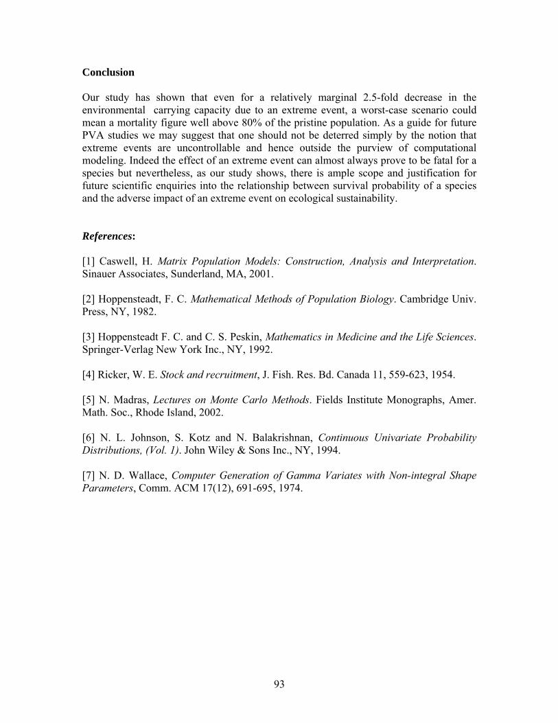
93

Conclusion Our study has shown that even for a relatively marginal 2.5-fold decrease in the environmental carrying capacity due to an extreme event, a worst-case scenario could mean a mortality figure well above 80% of the pristine population. As a guide for future PVA studies we may suggest that one should not be deterred simply by the notion that extreme events are uncontrollable and hence outside the purview of computational modeling. Indeed the effect of an extreme event can almost always prove to be fatal for a species but nevertheless, as our study shows, there is ample scope and justification for future scientific enquiries into the relationship between survival probability of a species and the adverse impact of an extreme event on ecological sustainability. References: [1] Caswell, H. Matrix Population Models: Construction, Analysis and Interpretation. Sinauer Associates, Sunderland, MA, 2001. [2] Hoppensteadt, F. C. Mathematical Methods of Population Biology. Cambridge Univ. Press, NY, 1982. [3] Hoppensteadt F. C. and C. S. Peskin, Mathematics in Medicine and the Life Sciences. Springer-Verlag New York Inc., NY, 1992. [4] Ricker, W. E. Stock and recruitment, J. Fish. Res. Bd. Canada 11, 559-623, 1954. [5] N. Madras, Lectures on Monte Carlo Methods. Fields Institute Monographs, Amer. Math. Soc., Rhode Island, 2002. [6] N. L. Johnson, S. Kotz and N. Balakrishnan, Continuous Univariate Probability Distributions, (Vol. 1). John Wiley & Sons Inc., NY, 1994. [7] N. D. Wallace, Computer Generation of Gamma Variates with Non-integral Shape Parameters, Comm. ACM 17(12), 691-695, 1974.

94

Processing Uncertainty and Indeterminacy in Information Systems Projects Success

Mapping

Jose L. Salmeron

Pablo de Olavide University at Seville

Spain

Florentin Smarandache

University of New Mexico

Gallup, USA

Abstract

IS projects success is a complex concept, and its evaluation is complicated, unstructured

and not readily quantifiable. Numerous scientific publications address the issue of

success in the IS field as well as in other fields. But, little efforts have been done for

processing indeterminacy and uncertainty in success research. This paper shows a formal

method for mapping success using Neutrosophic Success Map. This is an emerging tool

for processing indeterminacy and uncertainty in success research. EIS success have been

analyzed using this tool.

Keywords: Indeterminacy, Uncertainty, Information Systems Success, Neutrosophic

logic, Neutrosophic Cognitive Maps, Fuzzy logic, Fuzzy Cognitive Maps.

1. Introduction

For academics and practitioners concerned with computer-based Information Systems

(IS), one central issue is the study of development and implementation project success.

Literature (Barros et al., 2004; Poon and Wagner, 2001; Rainer and Watson, 1995;

95

Redmil, 1990) suggest that IS projects have lower success rates than other technical

projects. Irrespective of the accuracy of this presumption, the number of unsuccessful IS

projects are over the number of successful ones. Therefore, it is worthwhile to develop a

formal method for mapping success, since proper comprehension of the complex nature

of IS success is critical for the successful application of technical principles to this

discipline.

To increase the chances of an IS project to be perceived as successful for people involved

in project, it is necessary to identify at the outset of the project what factors are important

and influencing that success. These are the Critical Success Factors (CSF) of the project.

Whereas several CSF analyses appear in the literature, most of them do not have any

technical background. In addition, almost none of them focus on relations between them.

In addition, it is important to discover the relationships between them. Research about it

was becoming scarce.

In this paper, we propose the use of an innovative technique for processing uncertainty

and indeterminacy to set success maps in IS projects. The main strengths of this paper are

two-folds: it provides a method for processing indeterminacy and uncertainty within

success and it also allows building a success map.

The remainder of this paper is structured as follows: Section 2 shows previous research;

Section 3 reviews cognitive maps and its evolution; Section 4 is focused on the research

model; Section 5 presents and analyzes the results; the final section shows the paper’s

conclusions.

2. Previous research

Success is not depending to just one issue. Complex relations of interdependence exist

between IS, organization, and users. Thus, for example, reducing costs in an organization

cannot be derived solely from IS implementation. Studies indicate that the IS success is

hard to assess because it represent a vague topic that does not easily lend itself to direct

measurement (DeLone and McLean, 1992).

According to Zviran and Erlich (2003), academics tried to assess the IS success as a

function of cost-benefit (King and Schrems, 1978), information value (Epstein and King,

96

1983; Gallagher, 1974), or organization performance (Turner, 1982). System acceptance

(Davis, 1989) has used for it too. Anyway, cost-benefit, information value, system

acceptance, and organization performance are difficult to apply as measures.

Critical Success Factor method (Rockart, 1979) have been used as a mean for identifying

the important elements of IS success since 1979. It was developed as a method to enable

CEOs to recognize their own information needs so that IS could be built to meet those

needs. This concept has received a wide diffusion among IS scholars and practitioners

(Butler and Fitzgerald, 1999).

Numerous scientific publications address the issue of CSF in the IS field as well as in

other fields. But, little efforts have been done for introducing formal methods in success

research. Some authors (Poon and Wagner, 2001) analysed some aspects of CSF just by

the use of personal interviews, whereas others (Ragahunathan et al., 1989) carried out a

Survey-based field study. Interviews and/or questionnaires are common tools for

measuring success. However, formal methodology is not usual.

On the other hand, Salmeron and Herrero (2005) propose a hierarchical model to model

success. Anyway, indeterminacy was not processed. Therefore, we think that a formal

method to process indeterminacy and uncertainty in IS success is an useful endeavour.

3. Uncertainty and Indeterminacy processing in cognitive maps

3.1. Cognitive mapping

A cognitive map shows a representation of how humans think about a particular issue, by

analyzing, arranging the problems and graphically mapping concepts that are connected

between them. In addition, it identifies causes and effects and explains causal links (Eden

and Ackermann, 1992). The cognitive maps study perceptions about the world and the

way they act to reach human desires within their world. Kelly (1955, 1970) gives the

foundation for this theory, based on a particular cognitive psychological body of

knowledge. The base postulate for the theory is that “a person’s processes are

psychologically canalized by the ways in which he anticipates events.” Mental models of

97

top managers in firms operating in a competitive environment have been studied (Barr et

al., 1992) using cognitive mapping. They suggest that the cognitive models of these

managers must take into account significant new areas of opportunity or technological

developments, if they want stay ahead. In this sense, it is critical to consider mental

models in success research.

3.2. Neutrosophic Cognitive Maps (NCM)

In fact, success is a complex concept, and its evaluation is complicated, unstructured and

not readily quantifiable. The NCM model seems to be a good choice to deal with this

ambiguity. NCM are flexible and can be customised in order to consider the CSFs of

different IT projects.

Neutrosophic Cognitive Maps (Vasantha-Kandasamy and Smarandache, 2003) is based

on Neutrosophic Logic (Smarandache, 1999) and Fuzzy Cognitive Maps. Neutrosophic

Logic emerges as an alternative to the existing logics and it represents a mathematical

model of uncertainty, and indeterminacy. A logic in which each proposition is estimated

to have the percentage of truth in a subset T, the percentage of indeterminacy in a subset

I, and the percentage of falsity in a subset F, is called Neutrosophic Logic. It uses a subset

of truth (or indeterminacy, or falsity), instead of using a number, because in many cases,

humans are not able to exactly determine the percentages of truth and of falsity but to

approximate them: for example a proposition is between 30-40% true. The subsets are not

necessarily intervals, but any sets (discrete, continuous, open or closed or half-open/ half-

closed interval, intersections or unions of the previous sets, etc.) in accordance with the

given proposition. A subset may have one element only in special cases of this logic. It is

imperative to mention here that the Neutrosophic logic is a strait generalization of the

theory of Intuitionistic Fuzzy Logic.

Neutrosophic Logic which is an extension/combination of the fuzzy logic in which

indeterminacy is included. It has become very essential that the notion of neutrosophic

logic play a vital role in several of the real world problems like law, medicine, industry,

finance, IT, stocks and share, and so on. Fuzzy theory measures the grade of membership

or the non-existence of a membership in the revolutionary way but fuzzy theory has

98

failed to attribute the concept when the relations between notions or nodes or concepts in

problems are indeterminate. In fact one can say the inclusion of the concept of

indeterminate situation with fuzzy concepts will form the neutrosophic concepts (there

also is the neutrosophic set, neutrosophic probability and statistics).

In this sense, Fuzzy Cognitive Maps mainly deal with the relation / non-relation between

two nodes or concepts but it fails to deal with the relation between two conceptual nodes

when the relation is an indeterminate one. Neutrosophic logic is the only tool known to

us, which deals with the notions of indeterminacy.

A Neutrosophic Cognitive Map (NCM) is a neutrosophic directed graph with concepts

like policies, events, etc. as nodes and causalities or indeterminates as edges. It represents

the causal relationship between concepts. A neutrosophic directed graph is a directed

graph in which at least one edge is an indeterminacy denoted by dotted lines.

Let C1, C2,…, Cn denote n nodes, further we assume each node is a neutrosophic vector

from neutrosophic vector space V. So a node Ci will be represented by (x1, …,xn) where

xk’s are zero or one or I (I is the indeterminate introduced before) and xk = 1 means that

the node Ck is in the on state and xk =0 means the node is in the off state and xk = I means

the nodes state is an indeterminate at that time or in that situation.

Let Ci and Cj denote the two nodes of the NCM. The directed edge from Ci to Cj denotes

the causality of Ci on Cj called connections. Every edge in the NCM is weighted with a

number in the set {-1, 0, 1, I}. Let eij be the weight of the directed edge CiCj, eij Є {-

1,0,1,I}. eij = 0 if Ci does not have any effect on Cj, eij = 1 if increase (or decrease) in Ci

causes increase (or decreases) in Cj, eij = –1 if increase (or decrease) in Ci causes decrease

(or increase) in Cj. eij = I if the relation or effect of Ci on Cj is an indeterminate.

The edge eij takes values in the fuzzy causal interval [–1, 1] (eij = 0 indicates no causality,

eij > 0 indicates causal increase; that Cj increases as Ci increases and Cj decreases as Ci

decreases, eij < 0 indicates causal decrease or negative causality Cj decreases as Ci

increases or Cj, increases as Ci decreases. Simple FCMs have edge value in {-1, 0, 1}.

Thus if causality occurs it occurs to maximal positive or negative degree.

It is important to note that eij measures only absence or presence of influence of the node

Ci on Cj but till now any researcher has not contemplated the indeterminacy of any

relation between two nodes Ci and Cj. When we deal with unsupervised data, there are

99

situations when no relation can be determined between some two nodes. In our view this

will certainly give a more appropriate result and also caution the user about the risks and

opportunities of indeterminacy.

Using NCM is possible to build a Neutrosophic Success Map (NSM). NSM nodes

represent Critical Success Factors (CSF). They are the limited number of areas in which

results, if they are satisfactory, will ensure successful competitive performance for the

organization. They are the few key areas where “things must go right” for the project

(Rockart, 1979). This tool shows the relations and the fuzzy values within in an easy

understanding way. This is an useful approach for non-technical decision makers. At the

same time, it allows computation as FCM. Figure 1 shows the NSM static context.

Figure 1: NSM static context

5. Building a NSM

EIS project have been used for building a Neutrosophic Success Map. EIS, or executive

support systems as they are sometimes called, can be defined as computer-based

information systems that support communications, coordination, planning and control

functions of managers and executives in organizations (Salmeron and Herrero, 2005).

100

NSM will be based on textual descriptions given by EIS experts on interviews with them.

The steps followed are:

1) Experts selection. It is critical step. Expert selection was based on specific

knowledge of EIS systems. Experts are 19 EIS users of leading companies and

EIS researchers. The composition of the respondents is important. Multiple

choices were contemplated. The main selection criterion considered was

recognized knowledge in research topic, absence of conflicts of interest and

geographic diversity. All conditions were respected. In addition, respondents were

not chosen just because they are easily accessible.

2) Identification of CSF influencing the EIS systems.

3) Identification and assess of causal relationships among these CSF. Indeterminacy

relations are included.

Experts discover the CSFs and give qualitative estimates of the strengths associated with

causal links between nodes representing these CSFs. These estimates, often expressed in

imprecise or fuzzy/neutrosophic linguistic terms, are translated into numeric values in the

range –1 to 1. In addition, indeterminacy is used for modelling that kind of relations

relationships among nodes.

The nodes (CSFs) discover was the following:

1. Users’ involvement (x1). It is defined as a mental or psychological state of users

toward the system and its development process. It is generally accepted that IS

users’ involvement in the application design and implementation is important and

necessary (Hwang and Thorn, 1999). It is essential in maintenance phase too.

2. Speedy prototype development (x2). It encourages the right information needs

because it interacts between user and system as soon as possible.

3. Top management support (x3). EIS support with his/her authority and influence

over the rest of the executives.

4. Flexible system (x4). EIS must be flexible enough to be able to get adapted to

changes in the types of problems and the needs of information.

5. Right information requirements (x5). Eliciting requirements is one of the most

complicated tasks in developing EIS and getting a correct requirement set is

challenging.

101

6. Technological integration (x6). EIS tool selected must be integrated in companies’

technological environment.

7. Balanced development team (x7). Suitable human resources are required for

developing EIS. Technical background and business knowledge are needed.

8. Business value (x8). The system must solve a critical business problem. There

should be a clear business value in EIS use.

9. Change management (x9). It is the process of developing a planned approach to

change in a firm. EIS will be a new way of working. Typically the objective is to

maximize the collective efforts of all people involved in the change and minimize

the risk of failure of EIS project.

The NSM find out is presented in Figure 2. Fuzzy values are included.

Figure 2. EIS NSM

The adjacency matrix associated to NSM is N(E).

102

⎟⎟⎟⎟⎟⎟⎟⎟⎟⎟⎟⎟⎟

⎠

⎞

⎜⎜⎜⎜⎜⎜⎜⎜⎜⎜⎜⎜⎜

⎝

⎛

=

000000008.0000000108.0

7.004.01002.08.05.000007.0000

010000006.000000001.0

000000009.000002.000006.00000008.00

)(

I

IEN

The stronger relations are between x5 to x8, x7 to x5 and x8 to x3. It follows that a balanced

development team has a positive influence over elicitation requirements process. In the

same sense, eliciting right requirements have a positive influence over system business

value and system business value over top management support. In addition, users’

involvement receives influence from six nodes.

On the other hand, we have found two neutrosophic relations between x4 to x9, x5 to x3

and x7 to x9. It follows that experts perceive indeterminacy in relations between EIS

flexibility and balanced team skills to change management. They can not to assess the

relation between them, but they perceive that relation could exist. It is an useful

information since the decision-makers can be advised from it. They will be able to be

careful with those relations.

In addition, NSM predict effects of one or more CSFs (nodes) in the regarding ones. If

we know that any CSFs are on, we can discover the influence over the others. This

process is similar in Fuzzy Cognitive Maps.

Let ,..., , 13221 nn CCCCCC − be cycle (Vasantha-Kandasamy and Smarandache, 2003),

when Ci is switched on and if the causality flow through the edges of a cycle and if it

again causes Ci, we say that the dynamical system goes round and round. This is true for

any node Ci, for i = 1, 2,…, n. the equilibrium state for this dynamical system is called

the hidden pattern. If the equilibrium state of a dynamical system is a unique state vector,

then it is called a fixed point. If the NSM settles with a state vector repeating in the form

x1 → x2 → … → xi → x1,

then this equilibrium is called a limit cycle of the NSM.

103

Let C1, C2,…, Cn be the CSFs of an NSM. Let E be the associated adjacency matrix. Let

us find the hidden pattern when x1 is switched on when an input is given as the vector A1

= (1, 0, 0,…, 0), the data should pass through the neutrosophic matrix N(E), this is done

by multiplying A1 by the matrix N(E). Let A1N(E) = (a1, a2,…, an) with the threshold

operation that is by replacing ai by 1 if ai > k and ai by 0 if ai < k and ai by I if ai is not a

integer.

⎪⎪⎩

⎪⎪⎨

⎧

=⇒×==⇒×+=

=⇒>=⇒<

=

IaIcabaIcba

akaaka

kf

ii

ii

ii

ii

10

)(

This procedure is repeated till we get a limit cycle or a fixed point. According to this, the

limit cycle or a fixed point of vector state of each CSFs is calculated with k=0.5. We take

the state vector A1 = (1 0 0 0 0 0 0). We will see the effect of A1 over the model.

( ) ( ) 21 1000000116.00000008.00)( AENA =⎯→⎯=

( ) ( ) 232 1000000116.00002.0008.08.0)( AAENA ==⎯→⎯=

A2 is a fixed point. According with experts the on state of users’ involvement has effect

over speedy prototype development and change management.

We take the new state vector A1 = (1 0 1 0 0 0 0 0 0). We will see the effect of users’

involvement and top management support (A1) over the model.

( ) ( ) 21 1000001116.00002.0008.09.0)( AENA =⎯→⎯=

( ) ( ) 232 1000001116.00002.0008.07.1)( AAENA ==⎯→⎯=

Thus A2=(1 1 1 0 0 0 0 0 1), according with experts the on state of users’ involvement

and top management support have effects over the prototype speed of development (x2)

and change management (x9). It is interesting to discover that both previous state vectors

have the same influence over the model. Both vector states have influence over prototype

speed of development (x2) and change management, but no direct effect over the rest of

CSFs.

104

The vector states described are only two of the several available, even vectors with

several CSFs on. However the proposal here presented is as simple as possible while

being consistent with the process, data gathered from the expert’s perceptions, and the

aims and objectives of the paper.

6. Conclusions

The main strengths of this paper are two-folds: it provides a method for project success

mapping and it also allows know CSF effects over the other ones. In this paper, we

proposed the use of the Neutrosophic Success Maps to map EIS success.

A tool for evaluating suitable success models for IS projects is required due to the

increased complexity and uncertainty associated to this kind of projects. This leads to the

innovative idea of adapting and improving the existent Neutrosophic theories for their

application to indicators of success for IS projects.

Neutrosophic Success Map is an innovative success research approach. NSM is based on

Neutrosophic Cognitive Map. The concept of NCM can be used in modelling of systems

success, since the concept of indeterminacy play a role in that topic. This was our main

aim is to use NCMs in place of FCMs. When an indeterminate causality is present in an

FCM we term it as an NCM.

The results not mean that any CSF is unimportant or has not effect over the model. It

means what are the respondents’ perceptions about the relationships of them. This is a

main issue, since it is possible to manage the development process with more information

about the expectations of final users.

Anyway, more research is needed about Neutrosophic logic limit and applications.

Incorporating the analysis of NCM and NSM, the study proposes an innovative way for

success research. We think this is an useful endeavour.

105

References

[1] Axelrod, R. Structure of Decision: The Cognitive Maps of Political Elites, Princeton

Univ. Press, New Jersey, 1976.

[2] Barr P.S., Stimpert J.L. and Huff A.S. Cognitive Change, Strategic Action, and

Organizational Renewal, Strategic Management Journal 13 (1992), pp. 15-36.

[3] Barros, M.O.; Werner C.M.L. and Travassos, G.H. Supporting risks in software

project management, Journal of Systems and Software 70 (2004) (1-2), pp. 21-35.

[4] Butler, T. and Fitzgerald, B. Unpacking the systems development process: an

empirical application of the CSF concept in a research context, Journal of Strategic

Information Systems 8 (4) (1999), pp. 351–371.

[5] Davis, F. D. Perceived usefulness, perceived ease of use, and user acceptance of

information technology. MIS Quarterly 13 (1989) (3), pp. 319-340.

[6] Eastereby-Smith M., Thorpe R. and Holman D. 1996 “Using repertory grids in

management” Journal of European Industrial Training 20, p. 3.

[7] Eden, C. and Ackermann, F. 1992 “Strategy development and implementation – the

role of a group decision support system” in Holtham, C. Executive Information Systems

and Strategic Decision Support, Unicom, Uxbridge, UK, pp. 53-77.

[8] Epstein, B.J. and King W.R. An Experimental Study of the Value of Information,

Omega, 10(3) (1983), pp. 249-258.

106

[9] Gallagher, C.A. Perceptions of the Value of a Management Information System,

Academy of Management Journal, 17(1) (1974), pp. 46-55.

[10] Gordon M. and Tan F. 2002. “The repertory grid technique: A method for the study

of cognition in information systems”. MIS Quarterly 26(1), p. 39.

[11] Hwang, M.I. and, Thorn, R.G. The effect of user engagement on system success: a

meta-analytical integration of research findings, Information & Management 35 (4)

(1999) 229– 236.

[12] Kelly, G. 1970. “A brief introduction to personal construct theory”. Academic Press,

London.

[13] Kelly, G. 1955. “The Psychology of Personal Constructs”. New York, Norton &

Company.

[14] King, J.L. and Schrems, E.L. Cost-Benefits Analysis in IS Development and

Operation, Computing Surveys 10 (1978), pp. 19-34.

[15] Kosko, B. Fuzzy Cognitive Maps, Int. J. of Man-Machine Studies, 24 (1986) 65-75.

[16] Nord, J.H. and Nord, G.D. Executive information systems: a study and comparative

analysis, Information & Management 29 (2) (1995), pp. 95– 106.

[17] Poon P. and Wagner, C. Critical success factors revisited: success and failure cases

of information systems for senior executives, Decision Support Systems 30 (2001) (4),

pp. 393–418.

[18] Ragahunathan, T.S., Gupta, Y.P. and Sundararaghavan, P.S. Assessing the impact of

IS executives’ critical success factors on the performance of IS organisations.

Information and Management 17 (3) (1989), pp. 157–168.

107

[19] Rainer Jr. R.K. and Watson, H.J. The keys to executive information systems success,

Journal of Management Information Systems 12 (1995) (2), pp. 83– 98.

[20] Redmill, F. Considering quality in the management of software-based development

projects. Information & Software Technology 32 (1990) (1), pp.18-22.

[21] Rockart, J.F. Chief executives define their own data needs, Harvard Business

Review 57 (2) (1979) 81.

[22] Salmeron and Herrero, 2005. An AHP-based methodology to rank critical success

factors of Executive Information Systems. Computer Standards and Interfaces 28 (1). pp.

1-12

[23] Smarandache, F. A Unifying Field in Logics: Neutrosophic Logic, American

Research Press, Rehoboth, 1999. Available at http://

www.gallup.unm.edu/~smarandache/eBook-Neutrosophics2.pdf

[24] Turner, J.A. Firm Size, Performance and Computer Use, Proceedings of the Third

International Conference on Information Systems, Ann Arbor: University of Michigan,

(1982) pp. 109-120.

[25] Vasantha-Kandasamy, W.B. and Smarandache, F. Fuzzy Cognitive Maps and

Neutrosophic Cognitive Maps, Xiquan, Phoenix, 2003, Available at www.gallup.unm.

edu/~smarandache/NCMs.pdf

[26] Xirogiannis G., Stefanou J., and Glykas M. A fuzzy cognitive map approach to

support urban design. Expert Systems with Applications 26 (2004), pp. 257-268.

[27] Zviran, M. and Erlich, Z. Measuring IS user satisfaction: review and implications,

12(5) (2003), pp. 1-36.

108

Computational models pervade all branches of the exact sciences and have in recent

times also started to prove to be of immense utility in some of the traditionally 'soft'

sciences like ecology, sociology and politics. This volume is a collection of a few

cutting-edge research papers on the application of variety of computational models

and tools in the analysis, interpretation and solution of vexing real-world

problems and issues in economics, management, ecology and global politics by some

prolific researchers in the concerned fields. The Editors

7815999 730080

ISBN 1-59973-008-1

53995>