Computational Methods Matt Jacobson [email protected] Some slides borrowed from Jed Pitera...

Computational Methods

Matt Jacobson

[email protected]

Some slides borrowed from Jed Pitera (IBM, Adjunct Faculty UCSF)

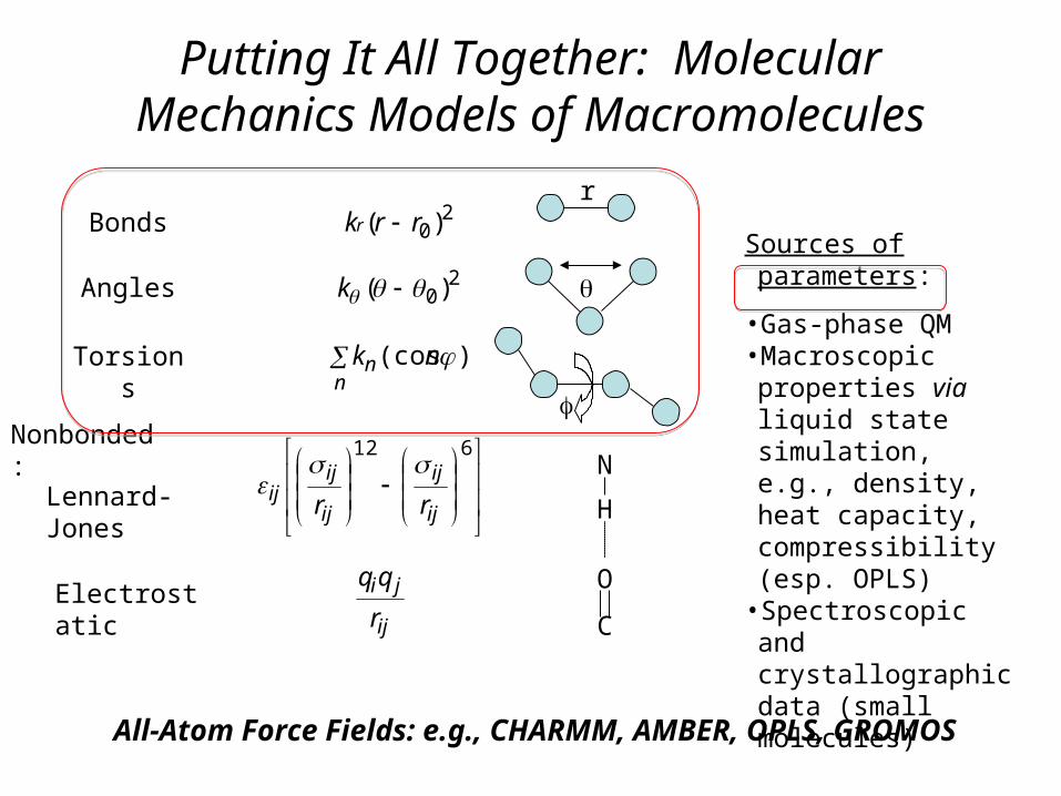
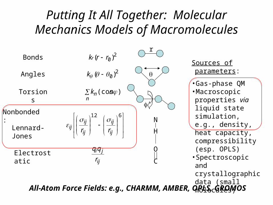
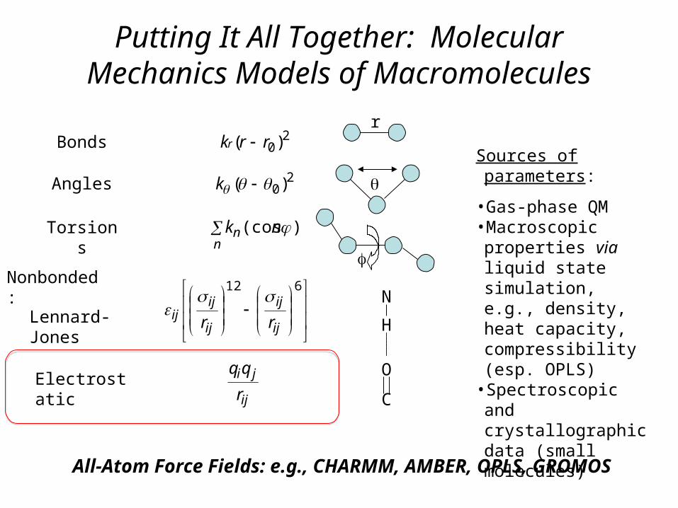
Molecular Mechanics Models of Macromolecules

All-Atom Force Fields: e.g., CHARMM, AMBER, OPLS, GROMOS

20)( rrkr Bonds

20)( k

n

n nk )(cos

Angles

Torsions

Nonbonded:

Lennard-Jones

ij

ji

r

qq

612

ij

ij

ij

ijij rr

Electrostatic

Sources of parameters:

•Gas-phase QM•Macroscopic properties via liquid state simulation, e.g., density, heat capacity, compressibility (esp. OPLS)

•Spectroscopic and crystallographic data (small molecules)

r

H

N

C

O

Putting It All Together: Molecular Mechanics Models of Macromolecules


20)( rrkr Bonds

20)( k

n

n nk )(cos

Angles

Torsions

Nonbonded:

Lennard-Jones

ij

ji

r

qq

612

ij

ij

ij

ijij rr

Electrostatic




r

H

N

C

O

Covalent forces are very strong

Bond Bond energy, kJ/mol

C–C 347

C=C 615

C≡C 812

C–O 360

C=O 728

F–F 158

Cl–Cl 244

C–H 414

H–H 436

H–O 464

O=O 498

1 , 2 bonds

1 , 1 bonds

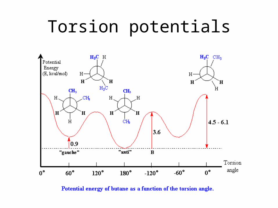
Torsion potentials



20)( rrkr Bonds

20)( k

n

n nk )(cos

Angles

Torsions

Nonbonded:

Lennard-Jones

ij

ji

r

qq

612

ij

ij

ij

ijij rr

Electrostatic




r

H

N

C

O

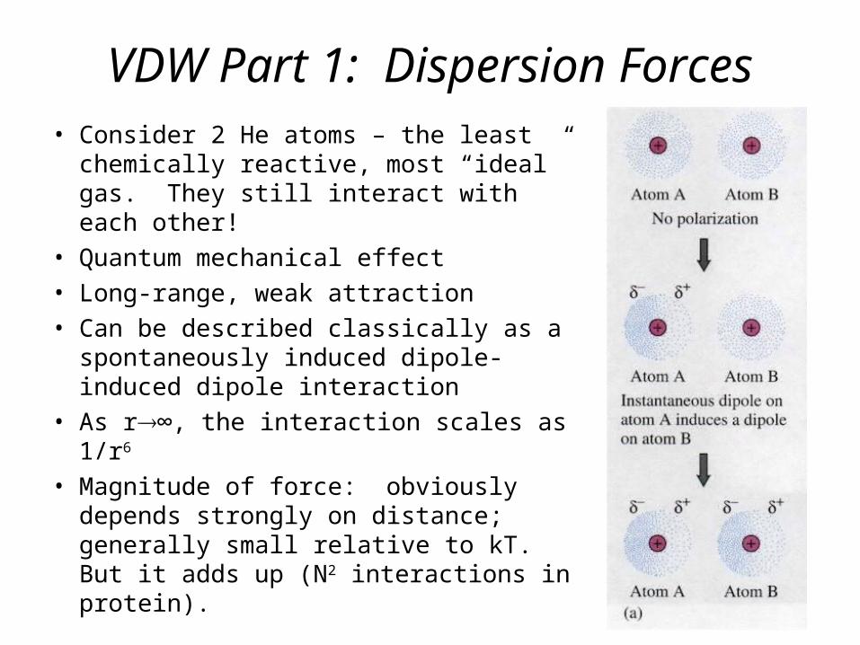
VDW Part 1: Dispersion Forces• Consider 2 He atoms – the least

chemically reactive, most “ideal” gas. They still interact with each other!

• Quantum mechanical effect• Long-range, weak attraction• Can be described classically as a

spontaneously induced dipole-induced dipole interaction

• As r∞, the interaction scales as 1/r6

• Magnitude of force: obviously depends strongly on distance; generally small relative to kT. But it adds up (N2 interactions in protein).

VDW Part 2: Close-Range Repulsion

• Direct consequence of Pauli exclusion principle: 2 electrons (which necessarily have same spin) cannot simultaneously occupy same space

• Formally increases exponentially with decreasing internuclear separation

• However, frequently modeled as 1/r12.• Magnitude of force: gets extremely large

very quickly (“steric clash”)

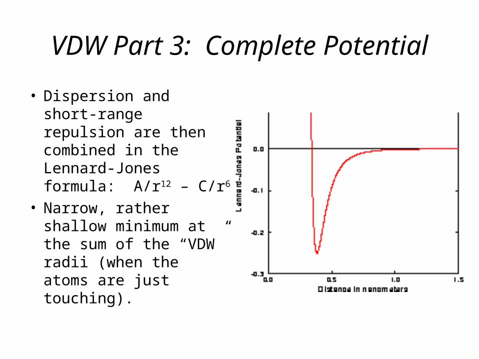
VDW Part 3: Complete Potential

• Dispersion and short-range repulsion are then combined in the Lennard-Jones formula: A/r12 – C/r6

• Narrow, rather shallow minimum at the sum of the “VDW” radii (when the atoms are just touching).



20)( rrkr Bonds

20)( k

n

n nk )(cos

Angles

Torsions

Nonbonded:

Lennard-Jones

ij

ji

r

qq

612

ij

ij

ij

ijij rr

Electrostatic




r

H

N

C

O

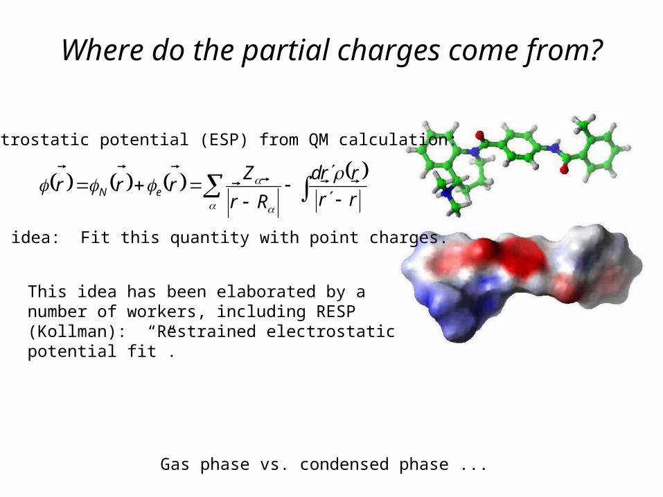
Where do the partial charges come from?

This idea has been elaborated by a number of workers, including RESP (Kollman): “Restrained electrostatic potential fit”.

rr

rrd

Rr

Zrrr eN

Electrostatic potential (ESP) from QM calculation:

Basic idea: Fit this quantity with point charges.

Gas phase vs. condensed phase ...



20)( rrkr Bonds

20)( k

n

n nk )(cos

Angles

Torsions

Nonbonded:

Lennard-Jones

ij

ji

r

qq

612

ij

ij

ij

ijij rr

Electrostatic


•Gas-phase QM•Macroscopic properties via liquid state simulation, e.g., density, heat capacity, compressibility


This is sufficient to describe a macromolecule by itself; but what about solvent?

r

H

N

C

O

Models of Solvation

Explicit

Pro: water models fairly mature

Con: ensemble averaging extremely expensive for large system

SPC, TIP4P, etc.

Adjustable parameters: Partial charges, bond lengths, etc.

+ –O

HHO

H H

OH

H

OHH

O HH

OH

H

OH

H

O

HH

O

HH

OH

H

O HH

Semi-analytical approximation

Implicit/Continuum

Pro: solvation free energy estimates cheap and generally accurate

Con: dynamics, first shell effects ???

Poisson-Boltzmann

Generalized Born

Adjustable parameters: radii

+ –

=80

=1

--

--

-- - + +

+++++

Heuristic

Distance-dependentdielectric

rr

i

iisolv AG

Surface-area based methods

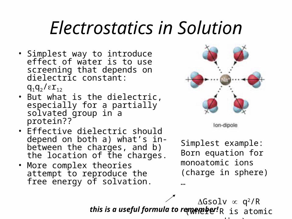
Electrostatics in Solution• Simplest way to introduce effect

of water is to use screening that depends on dielectric constant: q1q2/r12

• But what is the dielectric, especially for a partially solvated group in a protein??

• Effective dielectric should depend on both a) what’s in-between the charges, and b) the location of the charges.

• More complex theories attempt to reproduce the free energy of solvation.

Simplest example: Born equation for monoatomic ions (charge in sphere) …

Gsolv q2/R(where R is atomic radius)

this is a useful formula to remember!

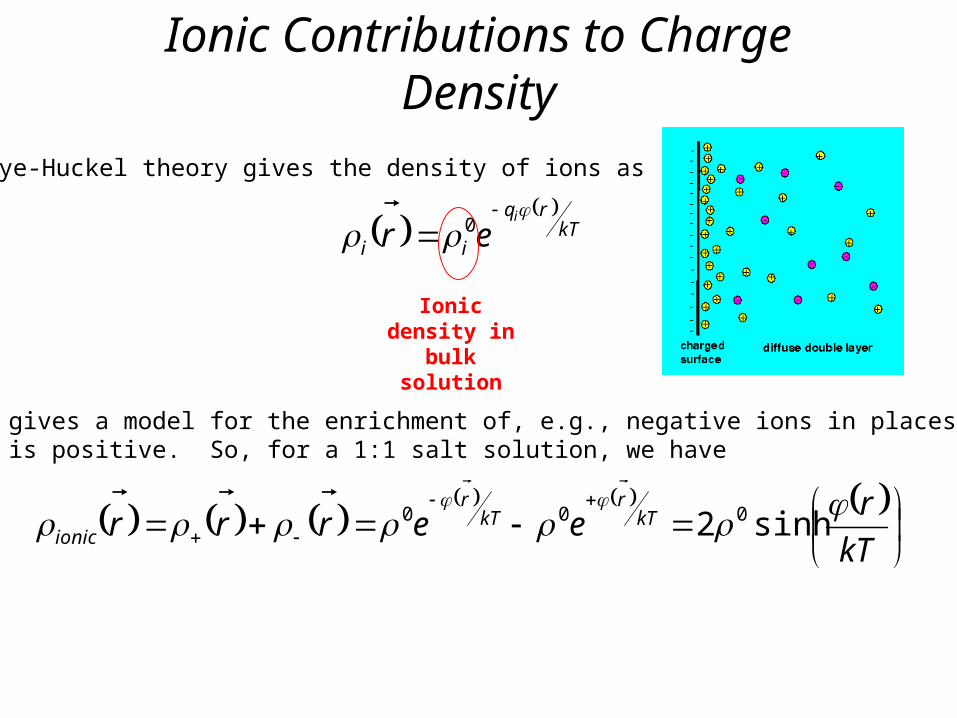
Ionic Contributions to Charge Density

Debye-Huckel theory gives the density of ions as

kTrq

ii

i

er

0

Ionic density in bulk solution

This just gives a model for the enrichment of, e.g., negative ions in places where the potential is positive. So, for a 1:1 salt solution, we have

kT

reerrr kT

rkT

r

ionic

sinh2 000

Many other types of “energy models” and “scoring functions” exist and are used for many applications

• small molecule docking• protein-protein docking• homology modeling• membrane permeability• protein dynamics/flexibility

Very frequently these models do attempt to capture certain aspects of the physics, but not generally as directly, or with as much generality, as force fields.

Empirical parameterization in most cases.

Main motivation: computational speed

Physics vs. empiricism

Questions I am frequently asked

• How good can I expect results to be from an MD simulation?

• Surely you should be able to compute a factor of 2 difference in binding affinity ...

• What’s the best force field?

Outline• Force fields• Molecular dynamics

– integrators– explicit solvent, periodic boundary conditions– a few applications

• Free energy methods– theory– alchemical perturbations– applications

Molecular Dynamics• Very simple idea: Just use the simple molecular mechanics models of

forces, then feed them into Newton’s equations of motion, basically F=ma. Then watch the molecules move!

• In the realm of biology, Martin Karplus deserves a lot of credit for early work that convinced people to think about macromolecules as dynamic, not static, structures. His program, Charmm, is still widely used.

• Now there are many thousands of papers using molecular dynamics, and lots of widely used programs.

• Some of the areas of current interest where MD continues to play an important role:

• Mechanisms of action of membrane proteins

• Mechanisms of allostery

• Protein folding

• Quantitative prediction of binding affinities• A nice review article: Karplus and McCammon, “Molecular dynamics

simulations of biomolecules”, Nat Struct Biol. 2002 Sep;9(9):646-52.

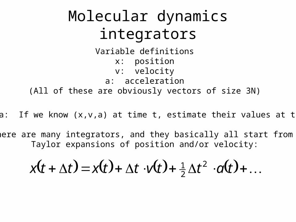
Molecular dynamics integrators

tattvttxttx 221

Variable definitionsx: positionv: velocity

a: acceleration(All of these are obviously vectors of size 3N)

Basic idea: If we know (x,v,a) at time t, estimate their values at time t+t

There are many integrators, and they basically all start from Taylor expansions of position and/or velocity:

Velocity Verlet integrator

This is not quite how it works in practice, but this is good enough for the problem set.

tattvttxttx 221

Position is updated first, based on current x, v, a

ttatattvttv 12

Velocity updates are more accurate if you use both the current/future acceleration. Q: How to get a(t + t)??A: Update positions, calculate new forces, use F=ma

Possible to play some tricks to get beyond 1 fs, e.g., freezing bonds, multiple timescale methods.

Currently limited to ~microsecond simulations now, soon getting up to milliseconds, probably, although these will be huge calculations, not something everyone can do. Typical simulations: nanoseconds.

Different representations of water

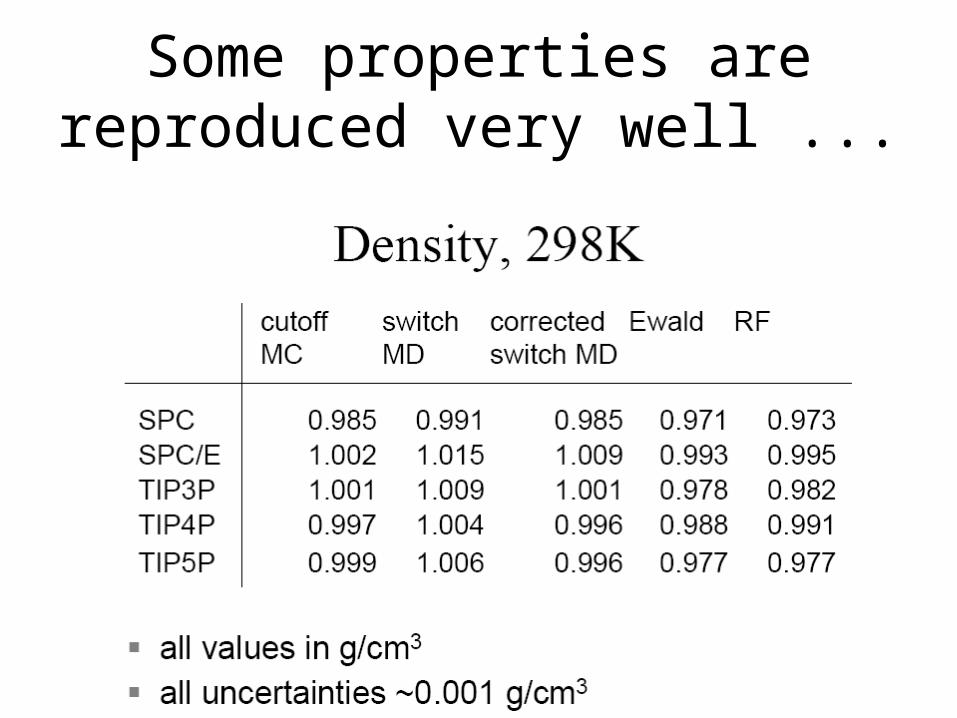
Some properties are reproduced very well ...

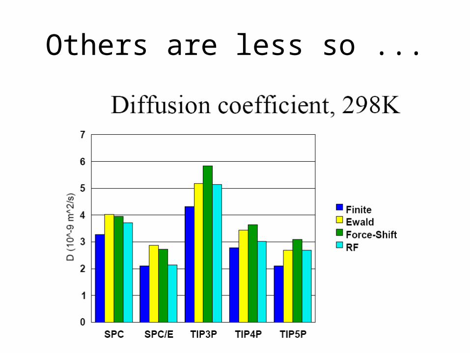
Others are less so ...

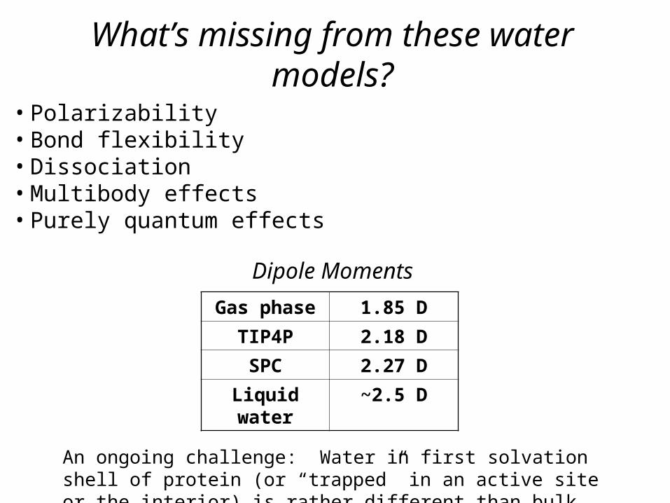
What’s missing from these water models?

• Polarizability• Bond flexibility• Dissociation• Multibody effects• Purely quantum effects

Gas phase 1.85 D

TIP4P 2.18 D

SPC 2.27 D

Liquid water ~2.5 D

Dipole Moments

An ongoing challenge: Water in first solvation shell of protein (or “trapped” in an active site or the interior) is rather different than bulk water.

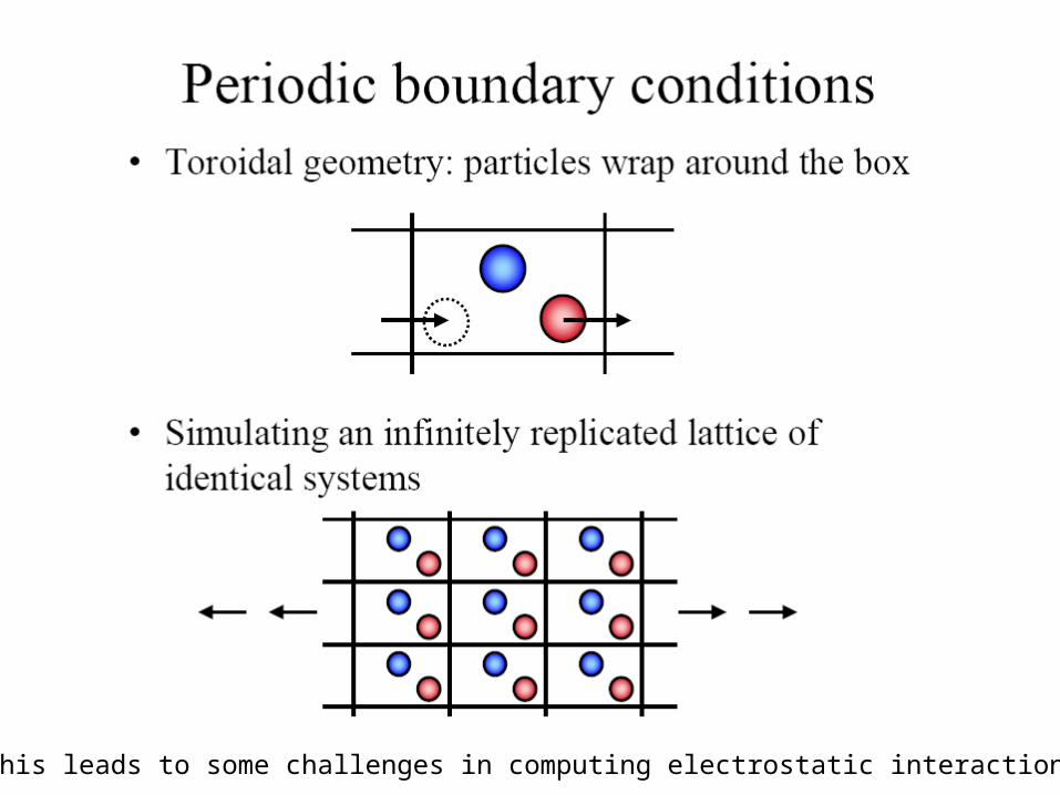
This leads to some challenges in computing electrostatic interactions

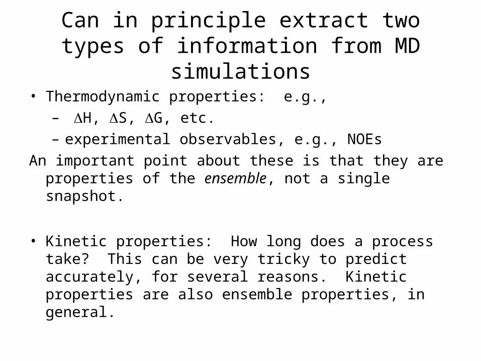
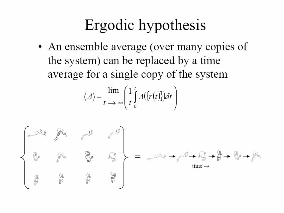
Can in principle extract two types of information from MD simulations

• Thermodynamic properties: e.g.,– H, S, G, etc.– experimental observables, e.g., NOEs

An important point about these is that they are properties of the ensemble, not a single snapshot.

• Kinetic properties: How long does a process take? This can be very tricky to predict accurately, for several reasons. Kinetic properties are also ensemble properties, in general.

Computational Methods Matt Jacobson [email protected] Some slides borrowed from Jed Pitera...

Documents

Transcript of Computational Methods Matt Jacobson [email protected] Some slides borrowed from Jed Pitera...