Purdue UniversityPurdue e-Pubs

Open Access Dissertations Theses and Dissertations

8-2016

Computational Labeling, Partitioning, andBalancing of Molecular NetworksBiaobin JiangPurdue University

Follow this and additional works at: https://docs.lib.purdue.edu/open_access_dissertations

Part of the Bioinformatics Commons, and the Systems Biology Commons

This document has been made available through Purdue e-Pubs, a service of the Purdue University Libraries. Please contact epubs@purdue.edu foradditional information.

Recommended CitationJiang, Biaobin, "Computational Labeling, Partitioning, and Balancing of Molecular Networks" (2016). Open Access Dissertations. 776.https://docs.lib.purdue.edu/open_access_dissertations/776

Graduate School Form30 Updated

PURDUE UNIVERSITYGRADUATE SCHOOL

Thesis/Dissertation Acceptance

This is to certify that the thesis/dissertation prepared

By

Entitled

For the degree of

Is approved by the final examining committee:

To the best of my knowledge and as understood by the student in the Thesis/Dissertation Agreement, Publication Delay, and Certification Disclaimer (Graduate School Form 32), this thesis/dissertation adheres to the provisions of Purdue University’s “Policy of Integrity in Research” and the use of copyright material.

Approved by Major Professor(s):

Approved by:

Head of the Departmental Graduate Program Date

Þ·¿±¾·² Ö·¿²¹

ÝÑÓÐËÌßÌ×ÑÒßÔ ÔßÞÛÔ×ÒÙô ÐßÎÌ×Ì×ÑÒ×ÒÙô ßÒÜ ÞßÔßÒÝ×ÒÙ ÑÚ ÓÑÔÛÝËÔßÎ ÒÛÌÉÑÎÕÍ

ܱ½¬±® ±º и·´±­±°¸§

Ó·½¸¿»´ Ù®·¾­µ±ªÝ¸¿·®

Ü¿·­«µ» Õ·¸¿®¿

Ø»²®§ Ýò ݸ¿²¹

Ö»²²·º»® Ò»ª·´´»

Ó·½¸¿»´ Ù®·¾­µ±ª

Ü¿±¹«± Ƹ±« éñêñîðïê

COMPUTATIONAL LABELING, PARTITIONING, AND BALANCING OF

MOLECULAR NETWORKS

A Dissertation

Submitted to the Faculty

of

Purdue University

by

Biaobin Jiang

In Partial Fulfillment of the

Requirements for the Degree

of

Doctor of Philosophy

August 2016

Purdue University

West Lafayette, Indiana

ii

Dedicated to my family

iii

ACKNOWLEDGMENTS

It is my great honor to be surrounded by many inspirational and friendly people

during my whole graduate study at Purdue. I first would like to thank my Ph.D.

advisor Michael Gribskov, for his unlimited encouragement over the years. His edu-

cational philosophy fosters a truly academic freedom that supports me to think about

the questions I am really interested in. I am also grateful to my committee members:

Daisuke Kihara, Henry Chang, and Jennifer Neville for their helpful comments. I

am also indebted to David Gleich for his numerous discussions on many technical

details of my research since he came to Purdue in 2011. I would also like to thank

Chun-Ju Chang for offering the collaboration opportunity which widens the scope of

my research. Of course, I cannot forget the supports from my research collaborators:

Yong Wang who led me to the field of bioinformatics, and Kyle Kloster for his patient

discussions and revision of our manuscript. Most of all, I owe my deepest gratitude

to my family for their endless love in my whole life.

iv

PREFACE

Computational biology is still in its infancy. It had not been included in any

college curriculum until the end of last century. That means every young researcher in

computational biology has his/her own story about how to transition to this new field

of study. Here, I would like to share my story about how I become a computational

biologist step by step.

My major in college was pharmaceutical engineering whose curriculum is a com-

bination of chemistry, chemical engineering and pharmacology. At that time, I had

very poor ability to keep tons of chemical reaction formulas in mind, and therefore

gained very little academic achievement in my major. In 2007, I accidentally regis-

tered a course on mathematical modeling when I was a sophomore. The first project

was to use mathematical models to predict the Chinese population in the future. I

still remember I used a logistic regression model to fit the given population data in

the past. As a result, my report received a top grade, which deeply encouraged me

to do something bigger in this field. In that summer, I founded a team with Yuanhai

Xue from computer science and Yongzhuo Li from optoelectronics to participate in

a five-round campus-wide competition in order to represent our college for the inter-

national contest. One of the problems we were given was to design a power supply

network that connects hundreds of villages with minimal lengths. Yuanhai taught

me Kruskal’s algorithm, a classical algorithm in graph theory for finding the minimal

spanning tree in a graph, to solve this problem. This was the beginning of my journey

in graph theory, and eventually led me to my graduate research: using network mod-

els to understand molecular functions and behaviors. Our team was finally awarded

meritorious winner in the international Mathematical Contest in Modeling in 2008,

and the two teammates become my lifelong friends.

v

After graduating from college, I went to the Academy of Mathematics and Sys-

tems Science in the Chinese Academy of Sciences as a research intern for one year,

under Yong Wang’s supervision. During that time, I utilized the PageRank algorithm

to study the relevance of proteins to Type 2 Diabetes in different tissues. At that

time, I wrote my first PageRank program using a very time-consuming power method.

Two years later, I took David Gleich’s class: Network and Matrix Computation, and

learned how to accelerate PageRank by formulating it as a linear system and solving

it faster by taking advantage of network sparseness. All these experiences benefit

my graduate research in this thesis about how to use PageRank to predict protein

functions and to partition a network into small modules. I suddenly realize that ev-

erything is ultimately interconnected, which reminds me of a speech given by Steve

Jobs at Stanford University in 2005:

“Again, you can’t connect the dots looking forward; you can only connect

them looking backwards. So you have to trust that the dots will somehow

connect in your future. You have to trust in something—your gut, destiny,

life, karma, whatever. Because believing that the dots will connect down

the road will give you the confidence to follow your heart even when it

leads you off the well-worn path and that will make all the difference.”

Biaobin Jiang

West Lafayette, Indiana

July 22, 2016

vi

TABLE OF CONTENTS

Page

LIST OF TABLES . . . . . . . . . . . . . . . . . . . . . . . . . . . . . . . . ix

LIST OF FIGURES . . . . . . . . . . . . . . . . . . . . . . . . . . . . . . . x

ABSTRACT . . . . . . . . . . . . . . . . . . . . . . . . . . . . . . . . . . . xii

1 Introduction . . . . . . . . . . . . . . . . . . . . . . . . . . . . . . . . . . 1

1.1 Network as a Language of Functions . . . . . . . . . . . . . . . . . 1

1.2 Network Construction . . . . . . . . . . . . . . . . . . . . . . . . . 5

1.2.1 Molecular Quantification . . . . . . . . . . . . . . . . . . . . 5

1.2.2 Interaction Measurement . . . . . . . . . . . . . . . . . . . . 8

1.2.3 Virtual Network Inference . . . . . . . . . . . . . . . . . . . 10

1.3 Network Topology . . . . . . . . . . . . . . . . . . . . . . . . . . . 12

1.3.1 Centrality . . . . . . . . . . . . . . . . . . . . . . . . . . . . 13

1.3.2 Distance . . . . . . . . . . . . . . . . . . . . . . . . . . . . . 14

1.3.3 Modularity . . . . . . . . . . . . . . . . . . . . . . . . . . . 16

1.4 Network Dynamics . . . . . . . . . . . . . . . . . . . . . . . . . . . 17

1.4.1 Edgetic Perturbation . . . . . . . . . . . . . . . . . . . . . . 18

1.4.2 Temporal Dynamics . . . . . . . . . . . . . . . . . . . . . . 19

1.5 Thesis Road Map . . . . . . . . . . . . . . . . . . . . . . . . . . . . 20

2 Network Labeling: Protein Function Prediction . . . . . . . . . . . . . . 22

2.1 Introduction . . . . . . . . . . . . . . . . . . . . . . . . . . . . . . . 23

2.2 Methods . . . . . . . . . . . . . . . . . . . . . . . . . . . . . . . . . 27

2.2.1 Problem Statement . . . . . . . . . . . . . . . . . . . . . . . 27

2.2.2 Preliminaries of Personalized PageRank . . . . . . . . . . . . 28

2.2.3 BirgRank: Bi-relational graph PageRank model . . . . . . . 31

2.2.4 Extension to AptRank . . . . . . . . . . . . . . . . . . . . . 33

vii

Page

2.2.5 Connection with Other Methods . . . . . . . . . . . . . . . . 35

2.3 Results . . . . . . . . . . . . . . . . . . . . . . . . . . . . . . . . . . 38

2.3.1 Experimental Setup . . . . . . . . . . . . . . . . . . . . . . . 38

2.3.2 Comparison of Prediction Performances . . . . . . . . . . . . 41

2.3.3 Analysis of Adaptive Coefficients . . . . . . . . . . . . . . . 46

2.3.4 Comparison of Runtimes . . . . . . . . . . . . . . . . . . . . 47

2.4 Conclusion . . . . . . . . . . . . . . . . . . . . . . . . . . . . . . . . 47

3 Network Partitioning: Functional Module Detection . . . . . . . . . . . . 52

3.1 Background . . . . . . . . . . . . . . . . . . . . . . . . . . . . . . . 53

3.2 Methods . . . . . . . . . . . . . . . . . . . . . . . . . . . . . . . . . 56

3.2.1 Localized PageRank Diffusion . . . . . . . . . . . . . . . . . 56

3.2.2 Finding Min-conductance Partition . . . . . . . . . . . . . . 58

3.2.3 Post-processing . . . . . . . . . . . . . . . . . . . . . . . . . 59

3.3 Results . . . . . . . . . . . . . . . . . . . . . . . . . . . . . . . . . . 60

3.3.1 Partitioning Protein Interactome . . . . . . . . . . . . . . . 60

3.3.2 Partitioning Gene Co-expression Network . . . . . . . . . . . 62

3.4 Conclusion . . . . . . . . . . . . . . . . . . . . . . . . . . . . . . . . 65

4 Network Balancing: Differential Flux Balance Analysis . . . . . . . . . . 67

4.1 Background . . . . . . . . . . . . . . . . . . . . . . . . . . . . . . . 67

4.2 Methods . . . . . . . . . . . . . . . . . . . . . . . . . . . . . . . . . 69

4.2.1 Model Assumption . . . . . . . . . . . . . . . . . . . . . . . 70

4.2.2 Model Construction . . . . . . . . . . . . . . . . . . . . . . . 70

4.2.3 Evaluation Metric . . . . . . . . . . . . . . . . . . . . . . . . 71

4.3 Results . . . . . . . . . . . . . . . . . . . . . . . . . . . . . . . . . . 72

4.3.1 Data Sets . . . . . . . . . . . . . . . . . . . . . . . . . . . . 72

4.3.2 Distribution of Differential Fluxes . . . . . . . . . . . . . . . 73

4.3.3 Identification of Known Cancer Genes . . . . . . . . . . . . 75

4.4 Conclusion . . . . . . . . . . . . . . . . . . . . . . . . . . . . . . . . 78

viii

Page

5 Side Projects . . . . . . . . . . . . . . . . . . . . . . . . . . . . . . . . . 80

5.1 Assessment of Subnetwork Detection Methods . . . . . . . . . . . . 80

5.1.1 Introduction . . . . . . . . . . . . . . . . . . . . . . . . . . . 80

5.1.2 Results . . . . . . . . . . . . . . . . . . . . . . . . . . . . . . 82

5.1.3 Conclusion . . . . . . . . . . . . . . . . . . . . . . . . . . . . 89

5.1.4 Methods . . . . . . . . . . . . . . . . . . . . . . . . . . . . . 90

5.2 SysTox Challenge: Classification of Smoking Exposure . . . . . . . 100

5.2.1 Introduction . . . . . . . . . . . . . . . . . . . . . . . . . . . 100

5.2.2 Methods: SVM, RF and ANN . . . . . . . . . . . . . . . . . 101

5.2.3 Results: Two-fold Cross Validation . . . . . . . . . . . . . . 103

5.2.4 Conclusion . . . . . . . . . . . . . . . . . . . . . . . . . . . . 106

6 Summary . . . . . . . . . . . . . . . . . . . . . . . . . . . . . . . . . . . 108

6.1 Discussion . . . . . . . . . . . . . . . . . . . . . . . . . . . . . . . . 108

6.2 Future Direction . . . . . . . . . . . . . . . . . . . . . . . . . . . . 108

6.2.1 All-in-One: Differential Pathway Analysis (DiPAna) . . . . . 108

6.2.2 Perspective . . . . . . . . . . . . . . . . . . . . . . . . . . . 109

LIST OF REFERENCES . . . . . . . . . . . . . . . . . . . . . . . . . . . . 111

VITA . . . . . . . . . . . . . . . . . . . . . . . . . . . . . . . . . . . . . . . 133

ix

LIST OF TABLES

Table Page

1.1 Thesis Outline . . . . . . . . . . . . . . . . . . . . . . . . . . . . . . . 21

2.1 Summary of the Six Methods . . . . . . . . . . . . . . . . . . . . . . . 49

2.2 Statistics of Data Sets . . . . . . . . . . . . . . . . . . . . . . . . . . . 50

2.3 Medians of γ in Prediction of Yeast and Human-2015 Data Sets . . . . 50

2.4 Runtimes of the Six Methods in Minutes (Human-2015 Dataset) . . . . 51

3.1 Statistics of Hi-C Contact Data in Mouse Chromosomes . . . . . . . . 63

3.2 Three Highlighted Modules Detected by BioSweeper . . . . . . . . . . . 65

5.1 Overview of the Eight Methods . . . . . . . . . . . . . . . . . . . . . . 94

5.2 Performance Summary of the Eight Methods. . . . . . . . . . . . . . . 95

5.3 Common Genes Identified by the Eight Methods . . . . . . . . . . . . . 96

5.4 Common Interactions Identified by the Eight Methods . . . . . . . . . 97

5.5 Parameter Setting of ANN . . . . . . . . . . . . . . . . . . . . . . . . . 105

x

LIST OF FIGURES

Figure Page

2.1 Distribution of Annotated Functions of Proteins. . . . . . . . . . . . . 28

2.2 Diffusion Patterns of Personalized PageRank. . . . . . . . . . . . . . . 30

2.3 Visualization of Given Data in a Simple Case. . . . . . . . . . . . . . . 32

2.4 Validation Strategy of Missing Function Prediction. . . . . . . . . . . . 40

2.5 Missing Function Prediction. . . . . . . . . . . . . . . . . . . . . . . . . 42

2.6 De novo Function Prediction. . . . . . . . . . . . . . . . . . . . . . . . 44

2.7 Guided Function Prediction. . . . . . . . . . . . . . . . . . . . . . . . . 45

3.1 Module Detection by Sweeping Over PageRank Vector. . . . . . . . . . 59

3.2 Distribution of PCC and PCC Squared. . . . . . . . . . . . . . . . . . 64

4.1 Scatter Plot of Protein Quantities and Fluxes in Normal vs. Cancer Con-ditions. . . . . . . . . . . . . . . . . . . . . . . . . . . . . . . . . . . . 73

4.2 Histogram of log2 Fold Changes in Protein Quantities and Fluxes. . . . 74

4.3 Fold Changes of Protein Quantities and Fluxes of 18 Hypermutated Genesin Colon Cancer. . . . . . . . . . . . . . . . . . . . . . . . . . . . . . . 76

4.4 ROC Curves in the Evaluation of Hypermutated Gene Prediction. . . . 77

4.5 AUROC in Robustness Test using Randomly Perturbed Networks. . . . 78

5.1 Volcano Plots of Differential Gene Expression. . . . . . . . . . . . . . . 84

5.2 ROC Curves of − log10(p-values) Predicting the Eight Subnetworks. . . 85

5.3 Modularity of the Eight Subnetworks. . . . . . . . . . . . . . . . . . . . 86

5.4 Prediction of the 462 Breast Cancer Genes by the Eight Subnetworks. . 87

5.5 Number of Methods Detecting Breast Cancer Genes and Interactions inSubnetworks. . . . . . . . . . . . . . . . . . . . . . . . . . . . . . . . . 98

5.6 Prominent Subnetwork Whose Interactions are Detected by At Least FiveMethods. . . . . . . . . . . . . . . . . . . . . . . . . . . . . . . . . . . 99

5.7 Performances of SVMs with Different Kernels. . . . . . . . . . . . . . . 103

xi

Figure Page

5.8 Performances of RF with Different Trees. . . . . . . . . . . . . . . . . . 104

5.9 Training Error of ANN. . . . . . . . . . . . . . . . . . . . . . . . . . . 106

5.10 Performance Comparison of the Three Methods. . . . . . . . . . . . . . 106

xii

ABSTRACT

Jiang, Biaobin Ph.D., Purdue University, August 2016. Computational Labeling, Par-titioning, and Balancing of Molecular Networks. Major Professor: Michael Gribskov.

Recent advances in high throughput techniques enable large-scale molecular quan-

tification with high accuracy, including mRNAs, proteins and metabolites. Differen-

tial expression of these molecules in case and control samples provides a way to select

phenotype-associated molecules with statistically significant changes. However, given

the significance ranking list of molecular changes, how those molecules work together

to drive phenotype formation is still unclear. In particular, the changes in molecular

quantities are insufficient to interpret the changes in their functional behavior. My

study is aimed at answering this question by integrating molecular network data to

systematically model and estimate the changes of molecular functional behaviors.

We build three computational models to label, partition, and balance molecular

networks using modern machine learning techniques. (1) Due to the incompleteness of

protein functional annotation, we develop AptRank, an adaptive PageRank model for

protein function prediction on bilayer networks. By integrating Gene Ontology (GO)

hierarchy with protein-protein interaction network, our AptRank outperforms four

state-of-the-art methods in a comprehensive evaluation using benchmark datasets.

(2) We next extend our AptRank into a network partitioning method, BioSweeper,

to identify functional network modules in which molecules share similar functions

and also densely connect to each other. Compared to traditional network parti-

tioning methods using only network connections, BioSweeper, which integrates the

GO hierarchy, can automatically identify functionally enriched network modules. (3)

Finally, we conduct a differential interaction analysis, namely difFBA, on protein-

protein interaction networks by simulating protein fluxes using flux balance analysis

xiii

(FBA). We test difFBA using quantitative proteomic data from colon cancer, and

demonstrate that difFBA offers more insights into functional changes in molecular

behavior than does protein quantity changes alone. We conclude that our integrative

network model increases the observational dimensions of complex biological systems,

and enables us to more deeply understand the causal relationships between genotypes

and phenotypes.

1

1. INTRODUCTION

The whole is greater than the sum of its parts.

—Aristotle (384–322 BC)

1.1 Network as a Language of Functions

A central goal of molecular biology is to understand molecular functions based on

sequences and structures. Sequences determine structures, and structures determine

functions, as a three-layer pyramid from bottom to the top. Sequences are molecular

identifiers indicating who the molecules are; structures are molecular appearances

showing what they look like; and functions are molecular vocations designating what

they do. Ultimately, evolution sheds light on why they do one thing and not an-

other. Understanding molecular functions serves as a genotype-phenotype mapping,

since a phenotype is a product of multiple molecular functions. Mapping genotypes

to phenotypes is not an easy task: one genotype may cause multiple phenotypes,

while one phenotype can originate from multiple genotypes. This many-to-many re-

lationship has been systematically mapped onto the Human Disease Network [1], in

which nodes are either a gene or a disease and edges are gene-disease associations.

The research group in this study published a drug-target network later in the same

year, which displays a similar intertwined relationship between drugs and their tar-

geted proteins [2]. Taken together, this disease-gene-protein-drug network implies

that characterizing molecular functions can close the gap between diseases and drugs

to transform traditional medicine with a one-disease-one-drug paradigm to precision

medicine with accurate diagnosis, personalized treatment, and predictive prevention.

How do molecular biologists investigate molecular functions? Half a century ago,

researchers believed that one gene genetically determines one enzyme that acts with

2

one function [3]. This simple concept leads to a reductionist research philosophy,

which has been dominant in molecular biology for a long time. A main reductionist

strategy in experimental design is to study the function of a single gene by deleting

the gene from the genome, and then comparing the phenotypic differences between

the mutant and a wild type control. On one hand, molecular biologists can manipu-

late genomic sequences to investigate the effects of genetic variants of many disease-

associated genes, especially for Mendelian diseases, a.k.a., monogenic diseases. On

the other hand, structural biologists can investigate structural variants of proteins

that cause diseases due to misfolding. However, this strategy fails if the expected

phenotypic difference is masked by compensation of another redundant gene with the

same function as the deleted one [4]. This property of robustness is one of the conse-

quences of evolution, which shapes the survival capability of organisms by exposure

to various deleterious environments, and builds up a living organism as an inseparable

whole. This suggests that a holistic strategy, which considers the living organism as

a whole, or as least as not just a single component, might be an alternative approach

to reductionism.

What is a holistic strategy, and how does molecular functional characterization

benefit from it? By definition, a holistic strategy is to study the interactions of the

multiple components of a complex system as an integrated system, rather than to

break it apart and study each part individually. The idea of holism was introduced

long ago, in the late 1940s, when scientists tried to interpret a systematic cellular

behavior: differentiation [5, 6]. Their question was “how can two cells, having ex-

actly the same genetic material, differentiate into two functionally different cells?”

The scientists interpreted differentiation as a positive feedback circuit in which two

molecules mutually activate each other. This system exhibits the property of bista-

bility : it tends to remain “on” once it is activated, and in contrast, remain “off”

once it is inactivated. This profound concept explains why two differentiated cells

are not interchangeable, and why the process of differentiation is rarely reversible.

Understanding a gene regulatory circuit, or gene regulatory network at large scale,

3

implies that understanding systematic cellular behaviors requires deep knowledge of

the complex interconnections between macromolecules, which brings up an emerging

field of study: systems biology.

The aim of systems biology is to study how complex interconnections between

macromolecules give rise to emergent cellular behaviors. There are no stringent defi-

nition of the scale and boundaries of a biological system. And therefore, a system can

be either as small as a signaling pathway, or as large as a whole organism. At local

levels, for instance, when one studies the function of a single transmembrane receptor

in detail, it can be beneficial to have a functional understanding of the binding ligands

in upstream and downstream signaling cascades in the pathway [7]. At intermediate

levels, a well-known example is the biochemical network in which nodes are metabo-

lites and edges represent biochemical reactions. Systems biologists use flux in the

biochemical network to denote reaction rates, and construct a linear programming

model called flux balance analysis (FBA, [8]) to simulate a steady state, or equilib-

rium, of the total network flux [9]. At the whole-cell level, the task becomes more

challenging since systems biologists need to consider not only a homogeneous network

wherein nodes are the same type (e.g., a metabolic network), but also a heterogeneous

network wherein nodes are of more than one type (e.g., transcription factors and their

targeted DNA sequences), or even networks of networks when simulating the entire

cell cycle [10].

Studying biomolecular networks can benefit pathology research by elucidating the

consequences of genetic variants. As mentioned above, the Human Disease Network

implies that dysfunction of one gene may result in multiple different diseases, and con-

versely, one multigenic disease may result from multiple genes. A common dilemma in

the study of disease-associated genotypes is that identical genetic variants are rarely

found across multiple patient samples with the same phenotype [11]. To this end,

Ciriello et al. proposed a computational method, called MEMo (Mutual Exclusivity

Modules), to identify highly recurrent genetic variants in the same biological process

(i.e., functional module, a subset of a biomolecular network) that are mutually exclu-

4

sive between different patients [12]. They claimed that, even though those variants

are not commonly found in all patients, they alter the same biological process, and

therefore, result in the same phenotype. Another example of using computational

network biology methods to address this dilemma is to infer tumor evolutionary tra-

jectories that illustrate which genetic variants drive the occurrence of others [13].

This method infers sequential networks between variants from longitudinal data, and

then performs network integration across different patient samples and uses network

deconvolution to determine a final resulting trajectory. Besides tumor heterogene-

ity, systems biologists also study the effects of genetic variants using protein-protein

binding interface data to increase the resolution of network interactions [14]. In a

profound study, Zhong et al. proposed a novel concept, namely edge-specific genetic

perturbation (edgetic perturbation) to denote a set of genetic variants that specifically

disrupt protein-protein interactions [15]. This study for the first time systematically

demonstrates how disease-associated variants cause loss of function at protein struc-

ture resolution (see Chapter 1.4.1 for details).

Given the effects of disease-associated genetic variants, as seen through the lens of

network data, systems biologists next seek a systematic treatment capable of restor-

ing the perturbations of those effects, which gives rise to a new field of study, namely

systems pharmacology or network medicine [16, 17]. To effectively develop drugs

targeting complex diseases, we may need to rewire signaling networks perturbed by

multiple genetic variants using a combinatorial treatment strategy. Irish et al. uti-

lized single-cell flow cytometry to monitor signaling activities of phospho-proteins,

and showed that there is dramatic remodeling of signaling networks between healthy

and acute myeloid leukemia patient samples [18]. Komurov et al. investigated a

set of breast cancer cells that are resistant to lapatinib treatment, an EGFR/ErbB2

inhibitor, and found that those cells receiving the treatment overly upregulate the

glucose deprivation network [19]. They next treated those cells with other drugs tar-

geting this network, which significantly reduces the survival rate of those resistant

cells. Furthermore, Lee et al. investigated this EGFR inhibition using a combina-

5

torial treatment strategy as well, and found that a sequential treatment of multi-

ple anticancer drugs, rather than simultaneous treatment, significantly enhances the

treatment effect of rewiring apoptotic signaling networks [20]. These successful ex-

amples suggests that modeling molecular networks can guide the design of multi-drug

combinatorial treatment to cure complex diseases caused by multiple genetic variants.

In summary, I have given a brief introduction to network biology, and how it en-

hances our understanding of multigenic diseases and provides therapeutic clues in the

development of combinatorial treatment. I next will further introduce how to con-

struct a molecular network via high throughput techniques, and how to computation-

ally analyze network topological structure, and its dynamics in disease progression.

1.2 Network Construction

A molecular network consists of multiple molecules and their interactions. In this

section, I will introduce several primary high throughput techniques for molecular

quantification and measurement of their interactions. In addition, I will introduce

computational methods for inference of virtual networks that cannot be measured

directly via experimental techniques.

1.2.1 Molecular Quantification

Proteins are primary functional units in a cell. Researchers are dedicated to de-

veloping a collection of qualitative and quantitative techniques to determine which

protein exits in the cell and how many copies it has. These techniques includes cel-

lular imaging, electron microscopy, array and chip platforms, and mass spectrometry

(MS) [21]. Unlike the other methods, mass spectrometry is a de novo analytic tech-

nique that examines complex protein populations, and it has been widely used in

pharmaceutical development, disease diagnosis and food safety control. In 2002, the

Nobel Prize in chemistry was jointly rewarded to John B. Fenn and Koichi Tanaka

for their exceptional contribution to the development of molecular ionization in mass

6

spectrometry. A generic mass spectrometry experiment consists of five steps [21]: (1)

isolate the proteins to be analyzed from cells or tissues; (2) digest the proteins to pep-

tides by trypsin; (3) ionize the peptides by electrospray or soft laser desorption; (4)

collect the mass/charge spectrum of the peptides; and (5) process the spectrum and

match the peaks against protein sequence databases to determine the identity of the

peptides. MS studies quickly go beyond qualitative to quantitative measurements,

enabling comparison of the same peptide under different experimental conditions.

Stable-isotope labeling by amino acids in cell culture (SILAC) tags peptides with

stable isotopes, such as 13C, 15N and 2H, to produce predictable mass differences

between peptides from two conditions [22]. Another quantitative method is targeted

MS techniques, e.g., Selected reaction monitoring (SRM) [23,24]. This method mon-

itors particular ions (ionized peptides) of an a priori known protein throughout a

tandem MS measurement over time, which enables the detection of low-copy number

proteins, and the quantitative study of its signaling behaviors.

Although detection and quantification of low-copy proteins is challenging [25],

and proteome-wide measurement based on current proteomic protocols are highly

laborious, large-scale proteome-wide measurements are technically possible for model

organisms, and even for human cells. Kim et al. introduced a draft map of the human

proteome using high-resolution Fourier-transform mass spectrometry [26]. Uhlen et

al. presented a map of the human tissue proteome including 44 major tissues and

organs in the human body using the integration of transcriptomics and antibody-

based proteomics [27]. The Cancer Proteome Atlas project has generated protein

expression data for many tumor samples using reverse-phase protein arrays (RPPAs),

which provides researchers with an insightful functional landscape of cancer proteomes

[28].

In addition to proteins, messenger RNAs (mRNAs) can also be measured in a high

throughput manner. RNA sequencing is a powerful technique for accurately measur-

ing gene expression at single-base resolution, and identifying different isoforms as

well [29]. Briefly, it first converts a long mRNA into a complementary DNA (cDNA),

7

and then fragments the cDNA into short sequences. After adding adaptors to the

two ends of each sequence, it utilizes high-throughput next-generation sequencing

technology to obtain the sequence of each cDNA fragment, a.k.a. reads. These reads

then can be mapped back to the reference genome, or are assembled together into

longer contigs in a de novo manner for species without reference genomes. The key

computational analysis in this RNA-seq transcriptomics pipeline is to accurately map

the reads to reference genomes. Numerous computational tools for RNA-seq assem-

bly and quantification have been developed in the past decade. A comprehensive

assessment has been conducted to evaluate the performances of 14 independent com-

putational methods using benchmark datasets [30]. It turns out that the current tools

can successfully identify transcript components with high accuracy, whereas accurate

identification of complete isoform structures still needs further improvement due to

the tremendous combinations of exons. Recently, a new ultra-fast method, namely

kallisto, has been proposed to quantify gene expression level from RNA-seq reads data

using pseudoalignment to avoid base-to-base exact alignment of reads to a reference

genome [31]. Experimental tests using both simulated and real datasets show that

kallisto achieves comparably accurate quantification with other four state-of-the-art

methods, but shortens the computational time by nearly 10 to 400 fold.

Another large class of biomolecules are metabolites. Metabolites can be mea-

sured and quantified using liquid chromatography and flow injection analysis-mass

spectrometry [32]. One computational analysis in metabolomics is to first identify

the associated proteins (e.g., enzymes) of the metabolites in the Human Metabolome

Database (HMDB) [33] , and then to analyze the regulatory pathways at the pro-

tein level. This method is suitable for small-scale studies of hundreds of metabolites.

Another method for large-scale studies is to reconstruct a metabolic network from

thousands of biochemical reactions, which usually requires community efforts [34].

The reconstruction of the global human metabolic network enables computational

analysis of each reaction rate using FBA, under the balanced assumption that the

8

current concentration of one metabolite is equal to the produced amount minus the

consumed amount.

Ultimately, systems biologists expect to comprehensively model and analyze the

physiological states of an individual using multi-omics data to fulfill the mission of

personalized medicine. Chen et al. presented an integrative personal omics profile

(iPOP) including genomic, transcriptomic, proteomic, metabolomic, and autoanti-

body profiles of an individual during 14 months [35]. This extensive study is the

first attempt to monitor an individual’s health using multi-omics data, and uncovers

various potential disease risks for useful guidance of prevention in advance.

1.2.2 Interaction Measurement

In order to understand the emergent properties of complex biological systems,

measuring molecular quantities alone is insufficient, since a biological system does

not run via simple summation of individual molecular functions, but via collective

behaviors mediated by molecular interactions.

The primary macromolecular interaction is protein-protein physical interactions

since proteins are the primary functional units in a cell. In 1989, Fields and Song

invented the yeast two-hybrid (Y2H) assay to successfully measure binary protein-

protein interactions [36]. The Y2H concept makes use of a reporter gene in yeast

for detecting the interaction of pairs of proteins inside yeast cell nucleus. First, a

bait protein and a prey protein are fused to a DNA-binding domain and a transcrip-

tional activation domain of a transcription factor (e.g., Gal4) via DNA recombination

techniques, respectively. Then if the bait protein binds to the prey protein, the two

domains of the transcription factor are linked to activate the expression of a reporter

gene (LacZ, encoding enzymes of galactose utilization) [36]. After a decade, two re-

search groups in 2000 presented large-scale Y2H screens identifying protein-protein

interactions in Saccharomyces cerevisiae (budding yeast) [37] and Caenorhabditis el-

egans (a roundworm) [38]. Giot et al. in 2003 and Rual et al. in 2005 used Y2H to

9

systematically map the first large-scale Drosophila melanogaster (fruit fly) and human

protein interactomes, respectively [39,40]. With continuous refinement and efficiency

improvement of the Y2H assays, researchers successfully map at larger scales the pro-

tein interactomes of S. cerevisiae in 2008 [41], C. elegans [42] and humans in 2014 [43].

Vo et al. presented a proteome-wide binary protein interactome for S. pombe (fission

yeast) comprising 2,278 interactions, conducted cross-species analysis of protein in-

teractomes, and identified more evolutionarily conserved interacting proteins between

S. pombe and humans, other than S. cerevisiae [44]. Marc Vidal and Stanley Fields

reviewed the history of Y2H from 1989, when Y2H was invented, to 2014 [45], and

estimated that, so far, about 10,000 high-quality binary protein-protein interactions

have been mapped, which accounts for less than 10% of the total protein interactome

in human.

Another technology for measuring protein-protein interactions is affinity purification-

mass spectrometry (AP-MS). This method is mainly used to measure interactions of

multi-protein complexes, the stoichiometry of the protein subunits, and dynamics of

the protein-complex assemblies [46]. In 1999, Bertrand Seraphin and his colleagues

developed the first AP-MS protocol in yeast [47]. The basic idea of AP-MS is first

to use an affinity reagent to purify a protein complex from a protein lysate, and then

to identify the subunits of the purified complex by MS. Some protein complexes with

a large number of subunits need to be purified multiple times using tandem affinity

purification (TAP) tags. Gavin et al. and Krogan et al. used the TAP-tag approach

followed by MS to comprehensively identify high-confidence interactions of protein

complexes in yeast [48, 49]. Hutchins et al. used AP-MS approach to systematically

identify human protein complexes during chromosome segregation [50]. Havugimana

et al. identified 622 human soluble protein complexes comprising 3,006 proteins and

13,993 high-confidence physical interactions [51]. The key difference between AP-MS

and Y2H is that AP-MS only gives a list of proteins physically associated with the

bait protein. How those subunits of protein complexes bind to each other cannot be

10

specified by AP-MS. That is why the interactions identified by Y2H are called binary

interactions.

In addition to identification of protein-protein interactions by Y2H and AP-MS in

single species, systems biologists utilize various high throughput techniques to identify

protein interactions between different species, or interactions of proteins with other

biomolecules. Rozenblatt-Rosen et al. used Y2H to map the interactions between tu-

mor virus proteins and host proteins, and found that tumor virus proteins systemati-

cally perturb the host interactome [52]. Breitkreutz et al. used MS-based approaches

to identify a kinase and phosphatase interaction (KPI) network comprising 1,844 in-

teractions in budding yeast [53]. Saliba et al. presented a liposome microarray-based

assay (LiMA) to systematically characterize protein-lipid interactions [54]. Gu et al.

invented a novel method for detecting protein-protein interactions by taking advan-

tage of powerful DNA sequencing technology [55]. Their single-molecule-interaction

sequencing (SMI-seq) attaches DNA barcodes to proteins so that the DNA barcodes

can next be amplified, sequenced and quantified by next-generation sequencing (NGS)

technology. To understand transcriptional regulation via binding of transcription fac-

tors and their direct targeting of DNA sequences, Johnson et al. presented a high

throughput method called chromatin immunoprecipitation followed by sequencing

(ChIPseq) for performing genome-wide mapping of protein-DNA interactions [56].

All these experimental methods aim to generate a global map of biomolecules, which

serves as the basis for further modeling and analysis of complex biological processes.

1.2.3 Virtual Network Inference

The biomolecular networks mapped by high throughput experimental assays are

still incomplete, and therefore, computational systems biologists attempt to construct

computational models to predict the interactions that have not been mapped by the

experimental assays using partially known interactions in current databases. Zhang

et al. devised a computational approach to predict protein-protein interactions using

11

three-dimensional structural information [57]. La and Kihara presented a phylo-

genetic framework, namely BindML, to predict protein-protein binding sites using

information from evolutionary conservation [58].

Another example of biological network inference is the identification of gene reg-

ulatory networks (GRNs). The interactions are “virtual”, which means that those

interactions do not necessarily imply a physical interaction between two genes, rather

than indirect interactions that arise from correlated patterns of gene expression [59].

Bansal et al. presented a comprehensive review on gene network inference algo-

rithms, and divided them into four classes: coexpression and clustering, Bayesian

networks (BNs), information-theoretic approaches, and ordinary differential equa-

tions (ODEs) [59]. Calculating Pearson correlation coefficients (PCCs) between each

pair of gene profiles is a straightforward method to construct a gene network. This

analytical framework is normally followed by a hierarchical clustering analysis to

group genes with similar expression profiles [60,61]. BNs are a graphical presentation

of the joint multivariate probability distribution that captures conditional indepen-

dence between random variables. Friedman et al. first constructed a BN to analyze

gene expression data in yeast, and successfully inferred several gene interactions that

are supported by biological evidences [62]. Information-theoretic approaches rely on

a statistical metric called Mutual Information (MI), which measures the degree to

which one random variable is non-randomly associated with another. Butte and Ko-

hane used MI to construct a relevance network using 79 expression measurements of

2,467 genes in yeast, and then detected 22 clusters of genes with significant biological

relevance [63]. ODEs are normally used to model time-series expression data without

considering statistical dependencies, in contrast to BN or MI. D’Haeseleer et al. used

ODEs to infer gene interactions given the expression of 65 genes at 28 time points,

and demonstrated how to use the resulting network to generate hypotheses and direct

further experiments [64]. To accelerate the development of novel methods for gene

network inference, systems biologists organized the Dialogue on Reverse Engineering

Assessment and Methods (DREAM) project, and integrated the inferred networks

12

from over 30 methods to produce a high-confidence network [65]. They further ex-

perimentally tested the ensemble network, and showed that 23 out of 53 previously

unreported interactions are supported by the experimental evidences.

To understand the properties of emergence and robustness of biological systems,

systems geneticists study the functional dependency of two genes by examining whether

the effects of simultaneously knocking out two genes is equal to the sum of the ef-

fects of the individual knockouts. This kind of functional dependency is referred to

as genetic interaction, or epistasis [66]. Tong et al. presented a high throughput

assay, termed synthetic genetic array (SGA) to systematically map the genetic inter-

action network in yeast comprising 204 genes and 291 interactions in 2001 [67]. They

continuously conducted the assays for a larger scale mapping of the yeast genetic

interactions including about 1,000 genes and 4,000 interactions later in 2004 [68]. In

2010, they finally created a global reference map for the yeast genetic interaction net-

work comprising 5.4 million gene-gene pairs using high throughput double knockout

assays [69]. Bandyopadhyay et al. further perturbed the yeast genetic interaction

network with a DNA-damaging agent, and found that the network rewires to adapt

to the external perturbation [70]. Another team utilized an RNA interference (RNAi)

strategy to comprehensively map the genetic interaction network in mammalian cells,

and created a functional map of chromatin complexes in mouse fibroblasts [71]. Those

extensive maps of functional dependency serve as a basis for system biologists to fur-

ther understand functional organization and adaptive properties of a cell.

1.3 Network Topology

Given a network, scientists have defined many topological properties from different

perspectives. Here, I will briefly introduce three basic network concepts: centrality,

distance, and modularity, and their applications to biological networks. In particular,

built on these three basic concepts, network scientists introduce the three most robust

13

measures of network topology: degree distribution, average path length and clustering

coefficient.

1.3.1 Centrality

The first and most straightforward network property is degree, the number of

connections (neighbors) that a node has in a network. Mathematicians and statistic

physicists attempted for a long time to find a probability distribution to fit the degree

distribution of a network. In 1959, the Hungarian mathematicians Erdos and Renyi

proposed a pure random network model with the assumption that each connection

(or edge) appears with equal probability, and is independent of any other connec-

tions [72]. This model produces a binomial distribution of network degree, or Poisson

distribution in the limit of large number of nodes. However, Barabasi et al. reported

in 1999 that most real-world networks, such as the internet and social networks,

follow a power-law distribution P (k) ∼ k−γ with 2 < γ < 3 [73], rather than the

Poisson distribution in the classical Erdos-Renyi model. They named the networks

following this power-law distribution scale-free networks, in the sense that the second

(variance) and higher moments of the power-law distribution are infinite when γ < 3,

and hence these networks lack a characteristic scale. In this type of network, a small

set of nodes have high degree, whereas the majority of nodes have low degree. They

explained this phenomenon by proposing a rule of network growth called preferen-

tial attachment : a new node prefers to attaching to the nodes with higher degree,

called hubs in the network [73]. This principle is commonly known as “the rich get

richer”. Several years later, many researchers showed that protein-protein interaction

networks are scale-free, following a power-law distribution [39–41, 49], even though

this statement is currently still in debate [74, 75]. These hub proteins were later

found to be essential in yeast: knockouts of hub genes frequently lead to lethality,

compared to non-essential genes/proteins with fewer links, whose removals are non-

lethal and tolerable [76]. Han et al. further defined two types of hubs: party hubs,

14

which interact with their partners at the same time and location, and date hubs,

which bind their neighbors at different times or locations [77]. By computationally

removing nodes to identify their topological importance, they found that both types

of hubs are indispensable to connectivity of the whole network, and date hubs are

even more significantly important than party hubs. Taylor et al. extended this con-

cept into intramodular hubs and intermodular hubs, and found that besides their

topological importance, intermodular hubs have more signaling domains and more

cancer-associated mutations than intramodular hubs [78].

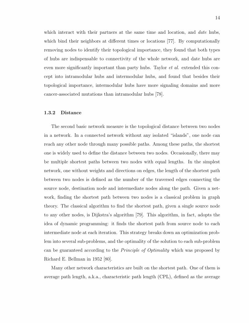
1.3.2 Distance

The second basic network measure is the topological distance between two nodes

in a network. In a connected network without any isolated “islands”, one node can

reach any other node through many possible paths. Among these paths, the shortest

one is widely used to define the distance between two nodes. Occasionally, there may

be multiple shortest paths between two nodes with equal lengths. In the simplest

network, one without weights and directions on edges, the length of the shortest path

between two nodes is defined as the number of the traversed edges connecting the

source node, destination node and intermediate nodes along the path. Given a net-

work, finding the shortest path between two nodes is a classical problem in graph

theory. The classical algorithm to find the shortest path, given a single source node

to any other nodes, is Dijkstra’s algorithm [79]. This algorithm, in fact, adopts the

idea of dynamic programming: it finds the shortest path from source node to each

intermediate node at each iteration. This strategy breaks down an optimization prob-

lem into several sub-problems, and the optimality of the solution to each sub-problem

can be guaranteed according to the Principle of Optimality which was proposed by

Richard E. Bellman in 1952 [80].

Many other network characteristics are built on the shortest path. One of them is

average path length, a.k.a., characteristic path length (CPL), defined as the average

15

length of all pairwise shortest paths in a network. CPL is widely used to characterize

the small-world phenomenon [81], popularly known as six degrees of separation [82].

Watts and Strogatz used CPL and clustering coefficient (see Chapter 1.3.3) to char-

acterize three real-world networks [83], and reported that the small-world networks

have longer CPL than the random networks (generated by the Erdos-Renyi model),

but smaller clustering coefficients than in lattice networks where each node connects

to its k nearest neighbors. In particular, a small-world network is defined as a net-

work whose CPL, termed L, increases proportionally to the logarithm of the number

of nodes N in the network, i.e., L ∝ logN . Telesford et al. proposed a unified small-

world measurement ω = Lrand/L − C/Clatt where C denotes clustering coefficient

and the subscripts “rand” and “latt” indicate random networks and lattice networks,

respectively [84]. CPL is widely used to quantify the topological importance of one

node in retaining the small-world property. A node is topologically important in re-

taining the small-world property if its removal increases the CPL of the network. As

mentioned previously, Taylor et al. used the change in CPL to show that intermodu-

lar hubs are more important in retaining the small-world property than intramodular

hubs [78].

Another network characteristic built on shortest paths is betweenness centrality,

another widely used centrality measure. The betweenness centrality of a node in a

network is defined as the number of all pairwise shortest paths that pass through that

node [85]. A node with high betweenness centrality is analogous to a bridge between

two big cities. And every time people would like to travel from one city to the other,

they have to pass through the bridge. Proteins with high betweenness are likely to

be essential: knocking out those genes tends to result in lethality [86]. Furthermore,

proteins with high betweenness but low degree tend to have low expression correlation

with their neighbors [86]. These proteins are likely to be key regulators in cross-

talk between two pathways. For example, cyclin-dependent protein kinase-activating

kinase 1 (CAK1) gene, encodes the protein Cak1p, which regulates two key signaling-

16

transduction pathways: the mitotic cell cycle, and the MAP kinase pathway which

regulates spore morphogenesis in yeast [86].

1.3.3 Modularity

A third network topological property is clustering coefficient, an indicator of mod-

ularity that partitions a global network into densely connected subnetworks. Even

though a holistic strategy attempts to investigate all molecules and their connections

as a whole, a global network sometimes may be too large to be analyzed without loss

of details. Partitioning a large network into several relatively independent modules

is a feasible compromise.

There are two different clustering coefficients: global clustering coefficient (GCC)

and local clustering coefficient (LCC). GCC is a characteristic of a network. Define

a triplet as three connected nodes in a network. A closed triplet is three nodes that

are fully connected by three edges, whereas an open triplet is three nodes that are

connected by two edges, without connection between one pair of nodes (open). Three

nodes in which one node lacks of connection are not considered to be a triplet. In 1949,

Luce and Perry defined GCC as the ratio of number of closed triplets over the total

number of triplets (both open and closed) [87]. GCC ranges from 0, indicating no

triplets, to 1 for a fully connected network. Similarly, LCC is a characteristic of nodes

in a network. LCC is defined as the ratio of number of edges between the neighbors

of a node over all possible edges between these neighbors. That is, a node having

k neighbors will have (k − 1)k/2 possible edges for the case of undirected networks.

A node whose neighbors are not connected to each other, like a spoke, will have an

LCC of 0, whereas a node with a fully connected neighborhood will have an LCC of

1. As mentioned previously, Watts and Strogatz defined a small-world network using

CPL and average LCC of all nodes, and demonstrated that a small-world network

has significantly higher average LCC than a random network [83].

17

Biological systems have proven to be modular [88]. Clustering coefficients can

only indicate whether a network is modular, and therefore, automatically finding func-

tional modules in biological networks has become a long-term goal in systems biology.

Ravasz et al. decomposed the metabolic networks of 43 distinct organisms into several

small but densely connected modules using an average-linkage hierarchical clustering

algorithm [60], and showed that those metabolic networks have higher average LCC

than module-free networks [89]. Girvan and Newman reviewed the shortcomings of

traditional hierarchical clustering methods in finding network modules. Based on this,

they proposed an alternative method using edge-betweenness [90]. They defined the

edge-betweenness of an edge as the number of pairwise shortest paths traversing that

edge divided by the number of all-pair shortest paths. And then they detected mod-

ules by sequentially removing the edges with high edge-betweenness. They further

proposed modularity, a score for quantifying the quality of functional modules [91].

It is defined as the observed number of edges within a module minus the expected

number of edges within the module. Assuming that each edge appears uniformly at

random, the expected number of edges between node i and j can be estimated as

kikj/2m, where ki and kj are the degrees of nodes i and j, and m is the total number

of edges in the network. Newman later proposed a spectral algorithm to maximize the

modularity score, and demonstrated that the proposed algorithm can detect better

modules with larger modularity scores than other modularity-based methods [92].

This problem has also gained the attention of computer scientists, since module

detection has become a general task not only in biological networks, but also social

networks and others. Fortunato gave a comprehensive review on the progress of this

study [93].

1.4 Network Dynamics

Network topology is primarily applied to characterizing static networks. However,

biological networks in many cases are not static, but dynamic [94]. Even though

18

high-throughput experimental technology for the interrogation of biological network

dynamics is still limited, accumulating evidence shows that biological networks rewire

when perturbed by genetic variants, or changes of post-translational modification

(PTM). Time-dependent molecular quantification can reveal quantitative changes in

interaction frequency and strength in signaling pathways. In this section, I will briefly

review experimental and computational techniques for examining biological network

rewiring and dynamics.

1.4.1 Edgetic Perturbation

As mentioned in Chapter 1.1, the concept of edgetic perturbation sheds light on

how genetic variants located in protein-protein binding interfaces disrupt specific

interactions rather than the entire protein structure [15]. Dreze et al. presented

an integrated method using the reverse Y2H system to systematically characterize

edgetic alleles of the gene CED-9, whose mutations can alter its protein-protein inter-

actions and result in different phenotypes in C. elegans [95]. Wang et al. investigated

62,663 genetic variants and their disruptive effects on 4,222 high-quality binary human

protein-protein interactions, and showed that different mutations in the same protein

can cause distinct disorders by altering different interactions [96]. In 2015, Sahni et

al. published a more comprehensive investigation with over 100,000 disease-associated

variants, and systematically characterized the effects of those human disease missense

mutations into two classes: protein folding/stability changes and protein interaction

perturbations [97]. In 2016, Yang et al. conducted a large-scale investigation on how

alternative splicing alters protein interactions, and demonstrated that besides genetic

mutations, different isoforms made by different combinations of exons, interact with

distinct functional partners in a tissue-specific manner [98]. This research team, led

by Marc Vidal at the Dana-Farber Cancer Institute, claimed in one review article

that the study of edgetics provides an insightful way to partially interpret genotype-

19

to-phenotype relationships as the loss or gain of protein interactions [99]. And they

named these edgetics-associated phenotypes as edgotypes.

Enlightened by the concept of edgetics, systems biologists have further explored

how genetic mutations alter signaling networks, e.g., phosphorylation-dependent in-

teractions between kinases and their substrates. Rune Linding and his colleagues

developed a computational method named KINspect to predict which amino acids in

the kinase domain determine substrate specificity [100], and then presented a compu-

tational framework called ReKINect, to analyze how genetic mutations of those alle-

les, termed network-attacking mutations, rewire phosphorylation-dependent signaling

networks leading to the associated phenotypes such as cancers [101]. AlQuraishi et al.

described an analytic framework based on multiscale statistical mechanics (MSM) to

estimate the effects of genetic mutations on the SH2 domains of human kinases, and

showed how those cancer-associated mutations mediate signaling pathways by acti-

vating or disrupting interactions [102]. All these studies demonstrate that the concept

of edgetics is not only applicable to common protein-protein physical interactions, but

also kinase-substrate transient interactions.

1.4.2 Temporal Dynamics

In addition to genetic mutations and PTMs, many other factors can alter molec-

ular interactions, such as molecular abundance, binding affinity, binding ratio (stoi-

chiometry), conditional regulation and so on. With the advance of high-throughput

molecular quantification during the past five years, it has become feasible to sys-

tematically quantify macromolecular abundance over time, even at the single-cell

level. In 2011, Tony Pawson and his colleagues designed an MS-based method named

AP-SRM, to quantify the changes in protein interactions with GRB2 (growth factor

receptor bound protein 2), an adaptor protein in the downstream of the epidermal

growth factor receptor (EGFR) pathway [103]. They successfully totally identified

90 proteins interacting with GRB2 in HEK293T cells at five different time points

20

after stimulation of cells with epidermal growth factor (EGF). This GRB2-centered

protein-interaction network displays a time-dependent map comprising upregulated,

downregulated, and unchanged interactions, and reveals the dynamic signaling be-

haviors from stimulation to activation of effectors.

In 2013, Ruedi Aebersold and his colleagues proposed another MS-based method,

called affinity purification combined with sequential window acquisition of all theo-

retical spectra (AP-SWATH), to investigate how the 14-3-3β scaffold protein changes

its interaction frequency with its binding partners after stimulation by insulin-like

growth factor 1 (IGF1) [104]. Lambert et al. at the same time developed the corre-

sponding statistical analysis pipeline for AP-SWATH, and applied it to investigating

the dynamics of another protein interactome centered at CDK4 (cyclin-dependent

kinase 4) under three different conditions: wild type, two mutants R24C and R24H,

and treatment by NVP-AUY922, an experimental drug candidate for cancers [105].

In 2014, Dana Pe’er, Garry Nolan and their colleagues pushed the study of molec-

ular interaction dynamics forward to single-cell resolution [106]. They utilized mass

cytometry, combined with the statistical models, to establish quantitative estima-

tion of signaling interaction strengths and the resulting signaling response functions

in naıve and antigen-exposed CD4+ T lymphocytes. They also experimentally val-

idated their estimated interaction strengths and demonstrated the utility of their

method in systematically mapping quantitative signaling networks.

1.5 Thesis Road Map

In this thesis, I develop three computational tools to investigate three topics in

network biology: labeling, partitioning, and balancing molecular networks. Due to the

incompleteness of protein functional annotations, I develop AptRank, a classification-

based method, to integrate molecular network data to predict protein functions.

With full molecular functional profiles, I next develop BioSweeper, a clustering-based

method, to partition the networks into functional modules in which molecules share

21

similar functions. Finally, I develop difFBA, a linear-programming-based method to

estimate the balanced state of protein fluxes throughout the network, and compare

the balanced states using proteomic data from healthy and colon cancer samples. The

organization of the three thesis projects is outlined in Table 1.1.

Table 1.1Thesis Outline

Chapter Topic Aim Tool

2 network labeling protein function prediction AptRank

3 network partitioning functional module detection BioSweeper

4 network balancing differential flux balance analysis difFBA

At the end, I briefly describe two side projects in Chapter 5, and summarize all

the works in Chapter 6.

22

2. NETWORK LABELING: PROTEIN FUNCTION

PREDICTION

Diffusion-based network models are widely used for protein function prediction

using protein network data and have been shown to outperform neighborhood-based

and module-based methods. Recent studies have shown that integrating the hierar-

chical structure of the Gene Ontology (GO) data dramatically improves prediction

accuracy. However, previous methods usually either used the GO hierarchy to refine

the prediction results of multiple classifiers, or flattened the hierarchy into a function-

function similarity kernel. No study has taken the GO hierarchy into account together

with the protein network as a two-layer network model.

We first construct a Bi-relational graph (Birg) model comprising protein-protein

association and function-function hierarchical networks. We then propose two diffusion-

based methods, BirgRank and AptRank, both of which use PageRank to diffuse infor-

mation on this two-layer graph model. BirgRank is a direct application of traditional

PageRank with fixed decay parameters. In contrast, AptRank utilizes an adaptive

diffusion mechanism to improve the performance of BirgRank. We evaluate the abil-

ity of both methods to predict protein function on yeast, fly, and human protein

datasets, and compare with four previous methods: GeneMANIA, TMC, Protein-

Rank and clusDCA. We design three different validation strategies: missing function

prediction, de novo function prediction, and guided function prediction to compre-

hensively evaluate predictability of all six methods. We find that both BirgRank and

AptRank outperform the previous methods, especially in missing function prediction

when using only 10% of the data for training.

AptRank naturally combines protein-protein associations and the GO function-

function hierarchy into a two-layer network model without flattening the hierarchy

into a similarity kernel. Introducing an adaptive mechanism to the traditional, fixed-

23

parameter model of PageRank greatly improves the accuracy of protein function pre-

diction. All the datasets and Matlab codes are available in our GitHub repository at

https://github.rcac.purdue.edu/mgribsko/aptrank.

2.1 Introduction

Given a set of functionally uncharacterized genes or proteins from a Genome-

Wide Association Study, or differential expression analysis, experimental biologists

often have little a priori information available to guide the design of hypothesis-based

experiments to determine molecular functions. For example, what is the expected

phenotype if a particular gene is removed? It would greatly improve hypothesis

formation if biologists had prior insight from predicted functions of interesting genes or

proteins in databases. Computational annotation of genes or proteins with unknown

functions is thus a fundamental research area in computational biology.

In the past decade, there has been much work to accurately predict functional

annotations of genes or proteins using heterogeneous molecular feature data [107,

108]. The collected molecular features include gene expression, sequence patterns,

evolutionary conservation profiles, protein structures and domains, protein-protein

interactions (PPIs), and phenotypes or disease associations. In one comprehensive

assessment [107], one of the methods, GeneMANIA [109] slightly outperformed the

other eight methods by integrating the multiple molecular features into a functional

association network (a.k.a., a kernel). The success story of GeneMANIA suggests two

important ideas. First, we can significantly improve prediction methods that rely on

a single data type by integrating data of many types. And second, kernel integration

is a particularly powerful approach to combining multiple types of data.

Given an integrated functional association network, methods for protein function

prediction can be divided into three different types: neighborhood-based, module-

assisted, and diffusion-based [110]. Neighborhood-based methods [111] predict the

function of one protein by using the functions of its neighbors in the network, i.e.,

24

the guilt-by-association approach. This approach has two obvious drawbacks. On

one hand, it ignores the functional information from all the other proteins outside the

neighborhoods of the query proteins, which leads to a low true-positive rate. On the

other hand, it may also have high false-positive rates when the query protein has a

single function but is surrounded by many multi-functional proteins.

Module-assisted methods operate by first partitioning a network or a kernel into

functional modules [112,113]. Biologically, a functional module in a PPI network is a

group of physically interacting proteins engaged in a biological activity, e.g., to form

a scaffold or to relay signals. In network science, a good module is commonly defined

as a densely connected subgraph with loose connections to the outside [91]. This

definition is naturally coincident with protein complexes, but not signaling cascades.

Obtaining a high-quality graph partition is challenging, and this field of study is still

highly active.

Diffusion-based methods generally simulate propagating information from func-

tionally known proteins to unknown ones through network connectivity. Nabieva et

al. [114] constructed a network flow model with fixed diffusion distances and capacities

on network edges. This method was claimed to capture both global network topology

as well as local network structure to improve the function predictability over the first

two domains of methods mentioned above. Freschi devised a tool called ProteinRank

by utilizing PageRank [115], the method used by Google to rank webpages, to dif-

fuse functional annotation information throughout a network without setting a fixed

diffusion distance or edge capacities [116]. Mostafavi et al. utilized the Label Prop-

agation algorithm [117] to develop GeneMANIA [109] as a classification model with

multiple heterogeneous network datasets using weighted kernels and labeled negative

samples. The method achieved approximately 70 ∼ 90% accuracy in three-fold cross

validation using a benchmark dataset [107]. Yu et al. [118] developed the Transduc-

tive Multilabel Classifier (TMC), based on a Bi-relational graph [119] consisting of

a protein interactome and cosine similarities in a protein functional profile as two

25

kernels in each graph layer. Then they used PageRank on this two-layer graph to

diffuse functional information to predict protein functions.

Functional annotation data are usually organized in a tree-like ontological struc-

ture with general terms at the root and specific terms on the leaves [120]. However,

the majority of previous methods disregard this intrinsic hierarchical structure by

assuming that the relationships between functions are independent. Recently, sev-

eral methods have been proposed in order to take into account the interdependent

relationships between functional terms in the hierarchical structure. King et al. [121]

predicted gene functions using decision trees and Bayesian networks while taking ad-

vantage of the annotation dependency between different branches of the GO hierarchy.

Notably, when they trained and tested the association of functional terms with genes,

they excluded the information from any ancestors and descendants of the terms in

question. This ensures a fair cross validation in which prediction does not benefit

from the GO annotation rule: if one gene is annotated by a term, then that gene is

automatically annotated by all the ancestors of that term. Barutcuoglu et al. [122]

and Valentini [123] proposed a hierarchical Bayesian framework and a True Path

Rule, respectively, to perform ensemble learning of the classification results yielded

by multiple Support Vector Machines (SVMs). They demonstrated that the accu-

racy of protein function prediction can be significantly improved by integrating the

functional hierarchy [124]. Tao et al. [125] and Pandey et al. [126] utilized Lin’s sim-

ilarity [127] to flatten the functional hierarchy, and then predicted protein functions

using a k-Nearest Neighbor (k -NN) method. Sokolov and Ben-Hur [128] directly mod-

eled the hierarchical structure of functional ontology using structured SVM [129], and

showed that their method outperformed k -NN and other binary classifiers without

taking the hierarchy into account. Recently, Yu et al. [130] combined Lin’s similarity

of protein functional profiles with an ontological hierarchy using downward random

walks with restarts, so as to improve the TMC model [118], which can predict func-

tions of a protein that are not in its neighborhood, but are present in the hierarchy.

Wang et al. proposed clusDCA [131] for protein function prediction by integrating

26

protein networks and a functional hierarchy, using PageRank for network smoothing

and low-rank matrix approximation to de-noise the network data.

In this study, we propose two methods that directly diffusing information on

the functional hierarchy other than a flat functional similarity constructed by Lin’s

method [127]. The first method, which we call BirgRank, constructs a Bi-relational

graph model with a protein-protein functional association network as one layer and an

unflattened ontological hierarchy as a second layer, and then directly applies PageR-

ank to diffuse annotation information across the two-layer network. The second

method, which we call AptRank, employs an adaptive version of PageRank that re-

places the standard PageRank parameters with values dynamically chosen to better

fit the training data. The main differences between our methods and other diffusion-

based methods are (1) we do not require any negative labeled samples since our

method is not a traditional classification model; (2) we take full advantage of the func-

tional hierarchy as a two-way directed graph, and do not use Lin’s similarity [127], or

any kernel trick, to flatten the hierarchy; and (3) we avoid using the annotation of a

particular term to predict the annotation of its parental terms, we train and test our

methods using the direct annotations only (see Figure 2.3(B) and (C)), which guar-

antees that the functional terms to be tested for each protein are mutually neither

ancestors nor descendants in the GO hierarchy.

To avoid the inflated accuracies of network-based methods in protein function

prediction noted by Gillis and Pavlidis [132–135], we conduct a large and strict evalu-

ation of our methods against the other state-of-the-art methods. In addition to three

small benchmark datasets, we use an up-to-date protein interaction network dataset

and exclude the functional annotations inferred from protein interactions (evidence

code: IPI). Rather than two-fold [116], three-fold [109, 131] or five-fold [118] cross

validation, we design three different validations: missing function prediction, de novo

function prediction, and a hybrid of the two strategies, namely guided function pre-

diction. For each of the three types of validation, we perform the validation method

using 20% or 10% of the data in training. To overcome the drawback of using Area

27

Under the ROC curve (AUROC) as a criterion in evaluating performance on imbal-

anced data with a small number of positive samples, we also utilize Mean Average

Precision (MAP) which focuses on the ranking of positive samples only, and is widely

used in the field of information retrieval.

2.2 Methods

2.2.1 Problem Statement

This study is motivated by the fact that there are still many proteins whose func-

tions are poorly characterized. To examine the extent to which each protein has

been experimentally annotated, we downloaded three benchmark datasets of yeast,

fly and human proteins maintained by GeneMANIA-SW since 2010 from their website

http://morrislab.med.utoronto.ca/~sara/SW/, and also the human Gene Ontol-

ogy Annotation (GOA) data [136] in March 2015. For the human GOA data, we

only consider the annotations in the Biological Process (BP) category, regardless of

Molecular Function (MF) and Cellular Component (CC) terms. Also, we only use

annotations with experimental evidence codes, within which we remove the terms in-

ferred by physical interaction (evidence code: IPI). All of these four datasets will be

used for evaluation later in this study. We illustrate the proportion of the number of

functional annotations of each protein in Figure 2.1. We can see that there are a large

number of proteins with fewer than 3 functional annotations. This is primarily due to

bias in biological research interests and the difficulty of experimentally determining

protein functions.

The aim of this study is to predict protein functions given a protein-protein associ-

ation network and a hierarchically structured set of functional terms. The hypothesis

is that associated proteins in the protein network are likely to share similar func-

tions. Here, we define a protein-protein association network as pairwise quantitative

relationships of proteins. This network either can be sparse and binary, e.g., a protein-

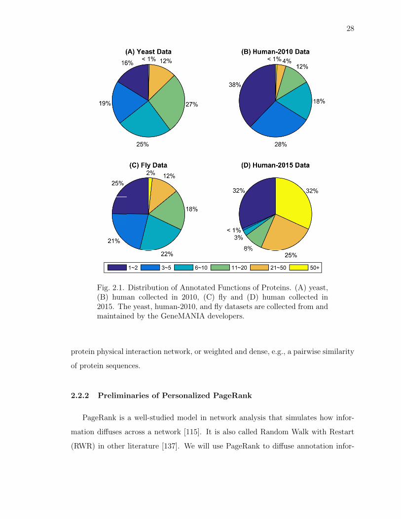
28

Fig. 2.1. Distribution of Annotated Functions of Proteins. (A) yeast,(B) human collected in 2010, (C) fly and (D) human collected in2015. The yeast, human-2010, and fly datasets are collected from andmaintained by the GeneMANIA developers.

protein physical interaction network, or weighted and dense, e.g., a pairwise similarity

of protein sequences.

2.2.2 Preliminaries of Personalized PageRank

PageRank is a well-studied model in network analysis that simulates how infor-

mation diffuses across a network [115]. It is also called Random Walk with Restart

(RWR) in other literature [137]. We will use PageRank to diffuse annotation infor-

29

mation from well-annotated proteins through a functional association network to less

well-annotated proteins. In particular, we use a “personalized” variation of PageR-

ank [138], which models the flow of information from a small number of specific

objects, called source nodes (in our case, a single protein) to the remainder of a net-

work. And we use this model to quantify which functions are most relevant to a

source protein.

Intuitively, personalized PageRank operates on a network of interconnected nodes

by placing a quantity of “dye” at a source node of interest, then letting the dye

diffuse across the edges of the network, decaying as it spreads. Once the diffusion

process decays to zero, the network regions where the largest amount of dye has

concentrated are then the most important regions to the source node. See Figure 2.2

for a visualization of the dye diffusing from a source node.

Mathematically, on a network with n objects, the network is modeled by an ad-

jacency matrix A ∈ Rn×n such that Aij is 1 if node j has an edge to node i, and is

0 otherwise. To model the diffusion process beginning with “dye” at a source node,

we use a vector v ∈ Rn×1 that is all 0s except for a 1 in the entry corresponding to

the source node. This vector v is called the personalization vector. Let x ∈ Rn×1

be a vector representing the amount of dye at each node in the network at some

point during the diffusion process. We then model the diffusion of the dye across the

graph by multiplying x by a column-stochastic version of A; this represents the dye

on node j being distributed in equal parts to each neighbor i of node j. We denote

the column-stochastic version of any nonnegative matrix M as M ; this is computed

by dividing each column of the matrix M by the sum of the entries in that column.

Finally, the decay of the diffusion process is controlled by the so-called PageRank

teleportation parameter, α ∈ (0, 1). During each stage of the diffusion, the dye that

spreads across the network decays proportionally to α, so that the amount of dye still

diffusing after k steps is αk. Then the PageRank vector x is given by the solution of

the linear system

(I − αA)x = (1− α)v. (2.1)

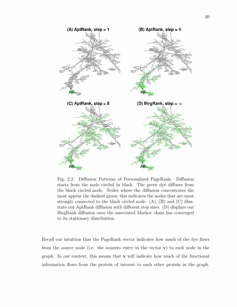
30

Fig. 2.2. Diffusion Patterns of Personalized PageRank. Diffusionstarts from the node circled in black. The green dye diffuses fromthe black circled node. Nodes where the diffusion concentrates themost appear the darkest green; this indicates the nodes that are moststrongly connected to the black circled node. (A), (B) and (C) illus-trate our AptRank diffusion with different step sizes. (D) displays ourBirgRank diffusion once the associated Markov chain has convergedto its stationary distribution.

Recall our intuition that the PageRank vector indicates how much of the dye flows

from the source node (i.e. the nonzero entry in the vector v) to each node in the

graph. In our context, this means that x will indicate how much of the functional

information flows from the protein of interest to each other protein in the graph.

31

In our model, we combine proteins and functions into a single network so that the

PageRank vector can indicate diffusion flow between proteins and functions.

The solution to the Personalized PageRank linear system in Equation (2.1) can

be expressed as

x =∞∑k=0

(1− α)αkAkv. (2.2)

This expression will become useful when we introduce the idea of using adaptive

coefficients in place of αk to optimize prediction quality (see Section 2.2.4). We note

that, although PageRank has an interpretation as a Markov chain, and Markov chains

must meet certain conditions to guarantee convergence to a stationary distribution,

this matrix power series (2.2) always converges for any α ∈ (0, 1) and stochastic

matrix A. Thus, the existence of the unique solution x is guaranteed regardless of

the structure of the matrix A. We emphasize this because the form of linear system

that we use differs from the traditional PageRank setting, which uses Markov chain

analysis in the proof of its convergence; in contrast, our computations do not rely on

this Markov chain analysis.

2.2.3 BirgRank: Bi-relational graph PageRank model

We denote the number of proteins by m and the number of function terms by n.

Then the three given datasets (protein-protein association network, protein-function

annotations, and function-function hierarchy) are denoted by the following matrices:

• G ∈ Rm×m, a symmetric matrix where G(i, j) denotes to which extent protein

i is associated with protein j;

• R ∈ Rm×n, a binary matrix where R(i, j) = 1 if protein i is annotated by

function j, 0 otherwise; and

• H ∈ Rn×n, a binary matrix where H(i, j) = 1 if functional term i is the child

of term j, 0 otherwise.

32

We illustrate these three components in Figure 2.3(A), (B) and (C), using a small ex-

ample with 6 proteins and 7 functional terms. For simplicity, Figure 2.3(A) shows a

protein-protein binary interaction network, but it can be replaced by any protein-

protein association network. Functional terms are hierarchically structured in a

Gene Ontology (Figure 2.3(C)) like an upside down “tree”, where the terms on the

top (root) are more general and the ones in the bottom (leaves) are more specific.

The annotation rule is that if one gene/protein is annotated by one term, then this

gene/protein is automatically annotated by all the parental terms of that term in the

hierarchy. However, note that in this study we only consider training and predict-

ing the direct annotations of each protein, and do not propagate the corresponding

parental annotations using the annotation rule, as shown in Figure 2.3(B). This en-

sures that our prediction does not benefit from the annotation rule.

A

B

C

E

F

D

0

2

3

1

4 5 6

G

HRT

0

A =

(A)

(C)

(B)

(D)

R

H

G

Fig. 2.3. Visualization of Given Data in a Simple Case. (A) protein-protein binary interaction network, (B) protein-function reference ma-trix, (C) function-function hierarchy, (D) adjacency matrix A of abi-relational graph.

33

Next, we construct a bi-relational graph [119] that incorporates these three datasets

into a single network (Figure 2.3(D)). To evaluate prediction performance, we split all

the annotations in R into RT , which we use for training during model construction,

and RE, which we use for evaluating predictions (see Figure 2.4). For each protein

i, we predict its functions using Equation (2.1) by setting it as the diffusion source,

i.e., by computing the diffusion using v = ei. To predict the functions of all proteins,

we extend the linear system in Equation (2.1) to a matrix form:Im 0

0 In

− α G 0

RTT H

XG

XH

= (1− α)

Im0

, (2.3)

where the bar over the block matrix still indicates the whole matrix is normalized to

be column-stochastic. The lower block of the solution, XH , is the output matrix of

BirgRank for function prediction, and has the same dimensions as RT . To further

control the proportion of diffusion passing between the two layers of the bi-relational

graph, we parameterize the model in Equation (2.3) asIm 0

0 In

− α µG 0

(1− µ)RTT H∗

XG

XH

= (1− α)

θIm

(1− θ)RTT

, (2.4)

whereH∗ = λH+(1−λ)HT , and λ controls the diffusion direction onH . Specifically,

λ = 0 indicates that the diffusion flows down the hierarchy, and 1 indicates flow up

the hierarchy. The parameter µ ∈ (0, 1) controls the proportion of the diffusion

flowing within G, and θ ∈ (0, 1) controls the weighted sources between the proteins

and functional annotations in the right-hand side of Equation (2.4).

2.2.4 Extension to AptRank

In the traditional model of PageRank, which we use in BirgRank, the teleporta-

tion parameter α ∈ (0, 1) can be thought of as controlling the rate of decay of the

diffusion as it spreads from the nodes in the personalization vector v to the rest of

the graph. After k steps the diffusion has decayed by a factor of αk, for k = 1, · · · ,∞

34

(Equation (2.2)). There are a variety of other empirical weighting schemes [139–142],

each with slightly different theoretical properties.

In this section, we seek to replace the standard, fixed diffusion coefficients αk at

each step with an adaptive parameter, denoted by γ(k), to optimize the predictive

power of the Markov chain. To do this we repeatedly split the training set of protein

function annotations, RT , into different subsets to use in fitting and validating the

coefficients. We denote the matrix used for fitting by RF , and the matrix used in

validation by RV . These matrices have the same dimensions as RT and consist of

entries of RT , i.e., RT = RF +RV .

To determine the adaptive coefficients γ(k) so that they bias predictions toward

the training data, we proceed as follows. The AptRank method begins by computing

terms in the following sequence:

X(k) =

X(k)G

X(k)H

=

G R∗F

RTF H∗

kX(0), (2.5)

where the bar over the block matrices still denotes column-stochastic normalization,

X(0) =

X(0)G

X(0)H

=

Im0

, (2.6)

and

R∗F =

0 to use a one-way diffusion

RF to use a two-way diffusion

.

We denote AptRank using a one-way diffusion and a two-way diffusion as AptRank-1

and AptRank-2, respectively. These two variations can have significant differences in

prediction performance when the underlying networks have different sparsities.

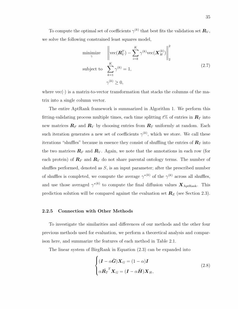
35

To compute the optimal set of coefficients γ(k) that best fits the validation set RV ,

we solve the following constrained least squares model,

minimizeγ

∥∥∥∥∥vec(RTV )−

K∑i=k

γ(k)vec(X(k)H )

∥∥∥∥∥2

2

subject toK∑k=1

γ(k) = 1,

γ(k) ≥ 0,

(2.7)

where vec(·) is a matrix-to-vector transformation that stacks the columns of the ma-

trix into a single column vector.

The entire AptRank framework is summarized in Algorithm 1. We perform this

fitting-validating process multiple times, each time splitting t% of entries in RT into

new matrices RF and RV by choosing entries from RT uniformly at random. Each

such iteration generates a new set of coefficients γ(k), which we store. We call these

iterations “shuffles” because in essence they consist of shuffling the entries of RT into

the two matrices RF and RV . Again, we note that the annotations in each row (for

each protein) of RF and RV do not share parental ontology terms. The number of

shuffles performed, denoted as S, is an input parameter; after the prescribed number

of shuffles is completed, we compute the average γ∗(k) of the γ(k) across all shuffles,

and use those averaged γ∗(k) to compute the final diffusion values XAptRank. This

prediction solution will be compared against the evaluation set RE (see Section 2.3).

2.2.5 Connection with Other Methods

To investigate the similarities and differences of our methods and the other four

previous methods used for evaluation, we perform a theoretical analysis and compar-

ison here, and summarize the features of each method in Table 2.1.

The linear system of BirgRank in Equation (2.3) can be expanded into(I − αG)XG = (1− α)I

αRTTXG = (I − αH)XH ,

(2.8)

36

Algorithm 1: AptRank

Input : G,RT ,H∗,K,S,t

Output: XAptRank

1 for s← 1 to S do

2 [RF , RV ] ← splitR(RT ,t)

// Choose t% of nonzero entries in RT uniformly at random and split to RF , and derive

RV = RT −RF .

3 Initialize X(0) using Equation (2.6)

4 for k ← 1 to K do

5 Compute X(k) using Equation (2.5)

6 A[:, k]← vec(X(k)H )

7 end

8 [QA,RA] ← qr(A) // QR decomposition

9 b ← vec(RV )

10 Solve

minimizeγ(s)

‖QTAb−RAγ

(s)‖22

subject to∑k

γ(s)k = 1, γ

(s)k ≥ 0

// Equivalently as Equation (2.7).

11 end

12 γ∗ ← median(γ(s))

// Take the median over all s = 1 to S for each k.

13

X∗GX∗H

← K∑k=1

γ∗k

G R∗T

RTT H∗

k Im0

14 Output XAptRank ←X∗H for use in prediction.

where G, RT , and H = H denote the submatrices of the column-stochastic matrix

in Equation (2.3). By solving Equations (2.8) for XH , we get

XH = α(1− α)(I − αH)−1RTT

(I − αG)−1. (2.9)

37

In contrast, ProteinRank [116] uses only the protein-protein association network

G as a one-layer network model — and does not directly take into consideration the

functional hierarchy H — and then computes PageRank using RT as the personal-

ization vectors (matrix). ProteinRank constructs a regression model and solves the

linear system

XProteinRank = (1− α)(I − αG)−1RT , (2.10)

which can cause poor prediction quality due to the assumption of independence be-

tween functions (see Section 2.3). Our method BirgRank is closely related to Protein-

Rank: if we plug H = I into Equation (2.9), then the resulting BirgRank solution

differs from the ProteinRank solution (Equation (2.10)) only by a scalar coefficient

and a slightly different normalization of G.

Similar to ProteinRank, GeneMANIA [109] models protein function prediction as

a multiclass-multilabel classification problem by integrating multiple heterogeneous

network datasets and then using the Label Propagation algorithm [117] as

XGeneMANIA = (I −L)−1R∗T , (2.11)

where L = D−W is the Laplacian matrix, W is a weighted sum of multiple kernel

matrices from heterogeneous network data sets, and D is a diagonal matrix with

Dii =∑

jWij. Additionally, GeneMANIA extends the binary matrix RTT to R∗T by

introducing negative samples in which R∗i,j = −1 if protein i is known not to have

function j. The developers of GeneMANIA further accelerated their algorithm by

introducing Simultaneous Weights (hereafter GeneMANIA-SW) [143].

Yu et al. proposed the Transductive Multilabel Classifier (TMC) [118] by di-

rectly applying a Bi-relational graph model used in image annotation [119] to protein

function prediction, without consideration of the functional hierarchy. Instead, they

use the cosine similarity of functional annotations to construct a function-function

similarity matrix to replace H . The key difference between TMC and BirgRank is

that TMC allows information to diffuse from functional terms to proteins, but not

38

proteins to functional terms, as in BirgRank. Mathematically, the transition matrix

of PageRank used in TMC is

ATMC =

WG WR

0 W F

, (2.12)

where the matrix W F is the degree-weighted function-function cosine similarity, i.e.,

cos(RTT ,RT ), WG is a degree-weighed graph kernel of protein-protein association

network, and WR is a normalized function profile derived from RT . The developers

of TMC suggest further flattening the functional hierarchy by using a random walk

with restart approach [130]. But this method, called dRW, does not use a bi-relational

graph model, and was tested only using a very small data set [130].

Wang et al. proposed clusDCA [131] by extending their original Diffusion Com-

ponent Analysis (DCA) method [144]. The clusDCA algorithm first uses PageRank

to smooth both of the graphs, denoted as G and H in this study. Next, it computes

Singular Value Decomposition (SVD) for the two smoothed matrices for low-rank

matrix approximations. Finally, it attempts to find the optimal projection between

the two low-rank matrices.

2.3 Results

2.3.1 Experimental Setup

We present a comprehensive evaluation of the six methods using the three bench-

mark datasets from yeast, human and fly that can be downloaded from the GeneMANIA-

SW website. All three datasets were collected by the developers of GeneMANIA in

2010. We collected one more dataset for human proteins from public databases in

March 2015 in order to test all the methods using up-to-date data with a larger

size than those collected in 2010 (see Table 2.2). In this human dataset, denoted

as human-2015, the network G was downloaded from BioGRID [145], and the an-

notations R and the hierarchy H from the Gene Ontology Consortium [136]. The

number of direct GO (Table 2.2, 3rd column) indicates the number of annotations of

39

individual proteins directly downloaded from the Gene Ontology Annotation (GOA)

database. This does not reflect the implied inclusion of parental terms (see the total

number of terms in Table 2.2, 4th column for comparison). The multiple kernels

(Table 2.2, 5th column) from heterogeneous molecular data were directly downloaded

from the GeneMANIA-SW website, and combined into a single network (i.e., G) with

the weights provided in the datasets.

To evaluate the quality of each method in protein function prediction, we con-

ducted cross validation using three different strategies to split the given functional

annotation data R into RT used for training and RE used for evaluation (see Sec-

tion 2.3.2). The three strategies are:

1. missing function prediction

2. de novo function prediction

3. guided function prediction.

All three validation strategies ensure that the matrices R, RT and RE have the same

dimensions, and R = RT +RE. To measure the prediction quality of each method,

we use two evaluation metrics: AUROC (Area Under the Receiver Operating Char-

acteristic curve) which is widely used in protein function prediction, and MAP (Mean

Average Precision) which is widely used in information retrieval (Figure 2.4). The

key advantage of MAP is that MAP does not take true negatives into account, and

is thus a more informative metric than AUROC when negative samples outnumber

positive samples. This is true in our case since in the human-2015 dataset, for exam-

ple, we attempt to predict 45 functions on average from 11, 519 possible annotations

(feature space, see Table 2.2).

We determined parameter settings as follows. For the four methods other than

our BirgRank and AptRank, we mostly used the default settings specified in the cor-

responding literature. We only tuned the reduced dimensionality d in clusDCA to

be 500, rather than the parameter setting 2, 500 specified by the authors [131], since

this parameter is a key factor in time complexity of clusDCA. Empirically, we found

40

Split

Train

Predict

Removal

R

RE

RT

X

Fig. 2.4. Validation Strategy of Missing Function Prediction. Splitthe given annotations R by putting 50% into the training set RT and50% into the evaluation setRE. Then compare the predictions againstRE and evaluate the performance of each method using AUROC andMAP.

that clusDCA is the most time-consuming method as shown in Table 2.4, and a large

d value dramatically increases running time. For the parameters in BirgRank, we set

λ = 0.5 in determining H∗, to allow equal diffusion upward and downward the hier-

archy. For the other three parameters α, θ, and µ in BirgRank (See Equation (2.4)),

we observed that different settings of these three parameters did not yield significant

differences in performance, and found that a value of 0.5 empirically achieved good

results. For the parameters in AptRank, we set the total iteration number K to be

8, the splitting parameter t to be 50%, and the number of shuffles S to be 5. These

setting may vary depending on the validation strategies and the data sizes, which we

discuss in Section 2.3.2.

41

2.3.2 Comparison of Prediction Performances

Missing Function Prediction

We first conducted a numerical experiment to evaluate the ability of the six meth-

ods in predicting missing protein functions as follows. We uniformly select a certain

percentage of non-zero entries in R at random, move them to a matrix RT for train-

ing, and let RE = R −RT be the evaluation set. Figure 2.4 illustrates how to split

matrix R with 14 entries into RT and RE when the splitting percentage is specified

as 50%. We carried out this random sampling with replacement 5 times for each

specified splitting percentage. This is not a circular cross validation since it does not

guarantee that each functional annotation is tested once and only once. This strategy

aims to test whether the methods can restore incomplete functional annotations for

each protein and is unbiased with respect to how many annotations each protein has.

We start with 10% split for training and increase by increments of 10% up to 80%

(Figure 2.5). Generally, the resulting AUROCs and MAPs of the six methods show

that both BirgRank and AptRank outperform the other four previous methods in all

8 groups of experiments with different amounts of training data. In the 10% group of

human-2010 and fly datasets, clusDCA slightly outperforms our methods in AUROC,

but its MAP is lower than those of our methods (Figure 2.5 (C) and (E)). When more

data are given for training, our methods outperform the other four methods in terms

of MAP with approximately 2- to 3-fold improvement.

To investigate the effect of the GO functional hierarchy in prediction, we com-

pare the performance of non-hierarchy-integrated methods (GeneMANIA-SW, TMC

and ProteinRank) with hierarchy-integrated methods (clusDCA, BirgRank and Ap-

tRank). We find that the integration of the functional hierarchy clearly improves the

prediction accuracy (Figure 2.5). Furthermore, our methods, for the most part, per-

form better than clusDCA, which suggests that using a bi-relational graph framework

(Figure2.3) to integrate the hierarchy is better than seeking for projection between

the protein network and the functional hierarchy.

42

10% 20% 30% 40% 50% 60% 70% 80%

AU

RO

C

0.6

0.7

0.8

0.9

1(A) Yeast Data

10% 20% 30% 40% 50% 60% 70% 80%

MA

P

0

0.25

0.5

0.75

1(B) Yeast Data

10% 20% 30% 40% 50% 60% 70% 80%

AU

RO

C

0.6

0.7

0.8

0.9

1(C) Human-2010 Data

10% 20% 30% 40% 50% 60% 70% 80%

MA

P

0

0.25

0.5

0.75

1(D) Human-2010 Data

10% 20% 30% 40% 50% 60% 70% 80%

AU

RO

C

0.6

0.7

0.8

0.9

1(E) Fly Data

10% 20% 30% 40% 50% 60% 70% 80%

MA

P

0

0.25

0.5

0.75

1(F) Fly Data

10% 20% 30% 40% 50% 60% 70% 80%

AU

RO

C

0.6

0.7

0.8

0.9

1(G) Human-2015 Data

10% 20% 30% 40% 50% 60% 70% 80%

MA

P

0

0.25

0.5

0.75

1(H) Human-2015 Data

GeneMANIA-SW TMC ProteinRank clusDCA BirGRank AptRank-1 AptRank-2

Fig. 2.5. Missing Function Prediction. The x -axis represents thepercentages of data used in training. The error mark on top of eachbar indicates the standard deviation of AUROCs or MAPs over 5repetitions of each experiment.

Comparing the performances of BirgRank and AptRank, we find that the perfor-

mance of the algorithms differs as the network sparsity varies (Figure 2.5 (B), (D),

(F) vs. (H)). The three benchmark datasets are smaller and denser than Human-2015

dataset due to the integration of multiple kernels (Table 2.2). We can see that Ap-

tRank with a two-way diffusion performs better on the dense network, while BirgRank

is better on the sparse network. This could be because a dense network restricts net-

work diffusion within a local region of the source node, and two-way diffusion forms a

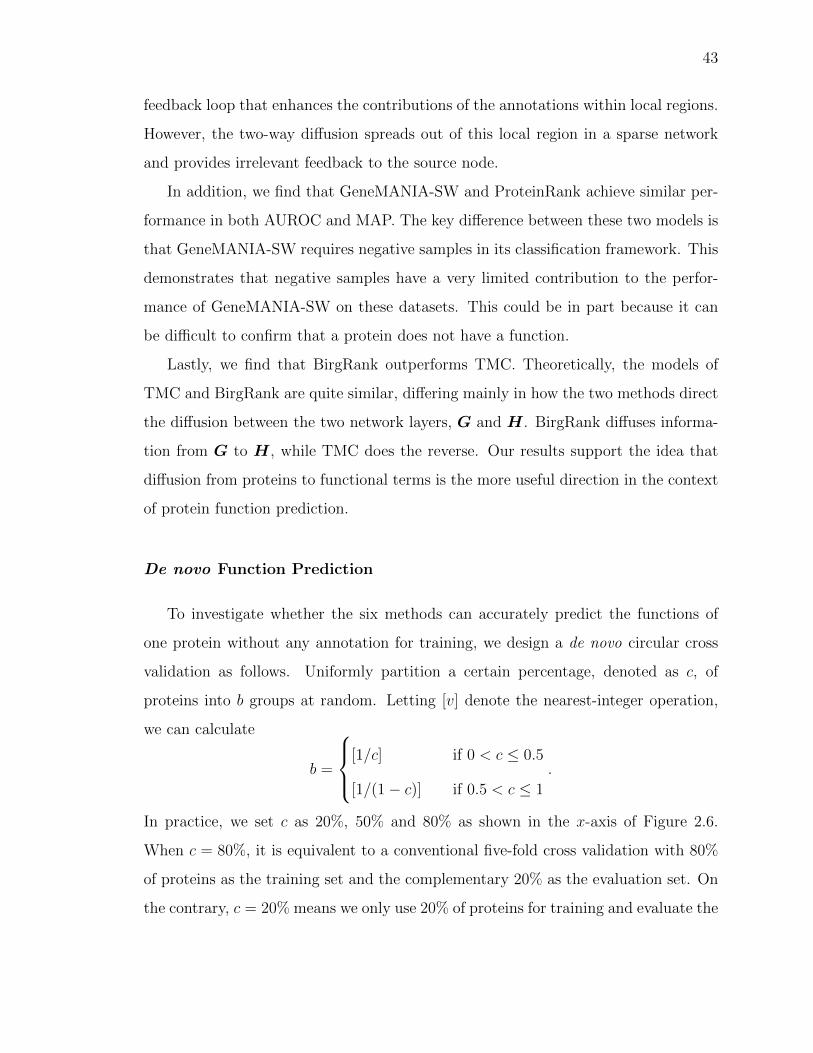
43

feedback loop that enhances the contributions of the annotations within local regions.

However, the two-way diffusion spreads out of this local region in a sparse network

and provides irrelevant feedback to the source node.

In addition, we find that GeneMANIA-SW and ProteinRank achieve similar per-

formance in both AUROC and MAP. The key difference between these two models is

that GeneMANIA-SW requires negative samples in its classification framework. This

demonstrates that negative samples have a very limited contribution to the perfor-

mance of GeneMANIA-SW on these datasets. This could be in part because it can

be difficult to confirm that a protein does not have a function.

Lastly, we find that BirgRank outperforms TMC. Theoretically, the models of

TMC and BirgRank are quite similar, differing mainly in how the two methods direct

the diffusion between the two network layers, G and H . BirgRank diffuses informa-

tion from G to H , while TMC does the reverse. Our results support the idea that

diffusion from proteins to functional terms is the more useful direction in the context

of protein function prediction.

De novo Function Prediction

To investigate whether the six methods can accurately predict the functions of

one protein without any annotation for training, we design a de novo circular cross

validation as follows. Uniformly partition a certain percentage, denoted as c, of

proteins into b groups at random. Letting [v] denote the nearest-integer operation,

we can calculate

b =

[1/c] if 0 < c ≤ 0.5

[1/(1− c)] if 0.5 < c ≤ 1

.

In practice, we set c as 20%, 50% and 80% as shown in the x-axis of Figure 2.6.

When c = 80%, it is equivalent to a conventional five-fold cross validation with 80%

of proteins as the training set and the complementary 20% as the evaluation set. On

the contrary, c = 20% means we only use 20% of proteins for training and evaluate the

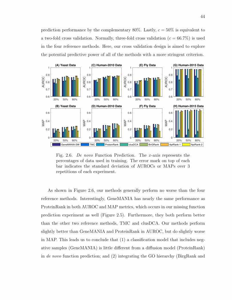
44

prediction performance by the complementary 80%. Lastly, c = 50% is equivalent to

a two-fold cross validation. Normally, three-fold cross validation (c = 66.7%) is used

in the four reference methods. Here, our cross validation design is aimed to explore

the potential predictive power of all of the methods with a more stringent criterion.

20% 50% 80%

AU

RO

C

0.6

0.7

0.8

0.9

1(A) Yeast Data

20% 50% 80%

MA

P

0

0.2

0.4

0.6

(B) Yeast Data

20% 50% 80%

AU

RO

C

0.6

0.7

0.8

0.9

1(C) Human-2010 Data

20% 50% 80%

MA

P

0

0.2

0.4

0.6

(D) Human-2010 Data

20% 50% 80%

AU

RO

C

0.6

0.7

0.8

0.9

1(E) Fly Data

20% 50% 80%

MA

P

0

0.2

0.4

0.6

(F) Fly Data

20% 50% 80%

AU

RO

C

0.6

0.7

0.8

0.9

1(G) Human-2015 Data

20% 50% 80%

MA

P

0

0.2

0.4

0.6

(H) Human-2015 Data

GeneMANIA-SW TMC ProteinRank clusDCA BirGRank AptRank-1 AptRank-2

Fig. 2.6. De novo Function Prediction. The x -axis represents thepercentages of data used in training. The error mark on top of eachbar indicates the standard deviation of AUROCs or MAPs over 3repetitions of each experiment.

As shown in Figure 2.6, our methods generally perform no worse than the four

reference methods. Interestingly, GeneMANIA has nearly the same performance as

ProteinRank in both AUROC and MAP metrics, which occurs in our missing function

prediction experiment as well (Figure 2.5). Furthermore, they both perform better

than the other two reference methods, TMC and clusDCA. Our methods perform

slightly better than GeneMANIA and ProteinRank in AUROC, but do slightly worse

in MAP. This leads us to conclude that (1) a classification model that includes neg-

ative samples (GeneMANIA) is little different from a diffusion model (ProteinRank)

in de novo function prediction; and (2) integrating the GO hierarchy (BirgRank and

45

AptRank) cannot significantly improve the accuracy in function prediction for newly

found proteins without known functional information.

Guided Function Prediction

To examine the extent to which our methods benefit from limited known an-

notations of tested proteins, we devise a validation strategy called guided function

prediction which is a hybrid of the missing function prediction (Section 2.3.2) and the

de novo prediction (Section 2.3.2) strategies. In this validation, the strategy of par-

titioning training and evaluation sets is identical to that used in de novo prediction

except that it gives one functional annotation as guidance for each evaluated protein

that has more than one annotation. The proteins in the evaluation set with only one

or no annotation are not taken into account.

20% 50% 80%

AU

RO

C

0.6

0.7

0.8

0.9

1(A) Yeast Data

20% 50% 80%

MA

P

0

0.2

0.4

0.6

(B) Yeast Data

20% 50% 80%

AU

RO

C

0.6

0.7

0.8

0.9

1(C) Human-2010 Data

20% 50% 80%

MA

P

0

0.2

0.4

0.6

(D) Human-2010 Data

20% 50% 80%

AU

RO

C

0.6

0.7

0.8

0.9

1(E) Fly Data

20% 50% 80%

MA

P

0

0.2

0.4

0.6

(F) Fly Data

20% 50% 80%

AU

RO

C

0.6

0.7

0.8

0.9

1(G) Human-2015 Data

20% 50% 80%

MA

P

0

0.2

0.4

0.6

(H) Human-2015 Data

GeneMANIA-SW TMC ProteinRank clusDCA BirGRank AptRank-1 AptRank-2

Fig. 2.7. Guided Function Prediction. The x -axis represents the per-centages of data used in training. The error mark on top of each barindicates the standard deviation of AUROCs or MAPs over 3 repeti-tions of each experiment.

46

We can see in Figure 2.7 that in the evaluations using the three benchmark datasets

with dense network data, our methods, especially AptRank-2, can take full advantages

of the single given annotation to improve prediction performance by approximately

2-fold in AUROC and 3-fold in MAP, compared to the other four methods. In the

sparse network data (Human-2015), we find that the given annotations worsen the

performances of all the methods (Figure 2.6 (G,H) vs. Figure 2.7 (G,H)). We con-

clude that sparse network datasets may cause underfitting of our model training, and

reducing the model complexity can alleviate this problem, e.g., setting a small α in

BirgRank or a small K in AptRank. On the contrary, we also find that in some

experiments, the more data we provide for training, the worse the testing accuracy

is (e.g., AptRank-2 in Figure 2.6(F)). In these cases, Verleyen et al. proposed using

sampling of the training data to overcome this overfitting [146].

Finally, all three validations show that AUROC is always higher than MAP in the

evaluation of the same prediction result. This suggests that MAP is a better metric

when the number of negative samples is much larger than the number of positive

samples, as is the case in protein function prediction.

2.3.3 Analysis of Adaptive Coefficients

The adaptive coefficients of AptRank (γ) are the unique feature that differs from

traditional PageRank. To investigate their behaviors in prediction, we list the medians

of γ over the different shuffles in the prediction of yeast and human-2015 datasets in

Table 2.3. We can see that there are three main features of γ’s behaviors,

(1) γ(1) is always zero, since the information diffusing within G, from proteins at the

first step, has not yet reached the hierarchy;

(2) as shown in the yeast dataset, the distribution of γ is not uniform, but concen-

trates on specific terms of Markov chains, which demonstrates that AptRank can

adaptively select the most predictive terms rather than weighting all terms with

power-decays like traditional PageRank; and

47

(3) in comparison of γ in yeast and human-2015 datasets, we find that AptRank

mostly selects the 2nd term in the human-2015 dataset, but a few more terms

in the yeast dataset, which is due to the different network densities of the two

datasets. The yeast dataset is smaller but denser, since it integrates 44 different

kernels into G; the human-2015 dataset is larger but sparser, and all the entries

in the raw human-2015 dataset are binary. This implies that for a sparse dataset,

our AptRank might be equivalent to neighbor-voting methods.

2.3.4 Comparison of Runtimes

The average computational time of the six methods compared in this study are

shown in Figure 2.4. In this comparison, the computational time is recorded for the

prediction using the largest dataset, human-2015. We can clearly see AptRank re-

quires the third longest computational time, likely because it involves many dense

matrix operations. The SVD computations required in clusDCA are likely responsi-

ble for clusDCA having the longest running time. Without a parallel implementation

of SVD, clusDCA might be impractical unless we sacrifice prediction accuracy by

using a small d value. GeneMANIA-SW is the second most computationally expan-

sive method, since it computes the prediction scores function by function. This is

extremely expensive when the number of functions is large, even though we only used

direct GO terms in GeneMANIA-SW. BirgRank and TMC both use bi-relational

graphs, and take only several minutes to solve the PageRank linear system. Protein-

Rank has the most simple model, and it takes the shortest time, since it needs only to

solve a PageRank linear system with approximately half the dimension of the systems

involved in BirgRank and TMC.

2.4 Conclusion

In this paper we present two network-diffusion-based methods for protein function

prediction. Our first method, BirgRank, uses PageRank on a bi-relational graph

48

model that incorporates protein-protein and function-function networks. Our second

method, AptRank, introduces an adaptive mechanism to the PageRank framework

that computes an optimal set of weights for the first several steps of diffusion so as

to maximize recovery of a subset of known function annotations. We show that both

methods outperform the four existing state-of-the-art methods in almost all cases,

and in particular, outperform those methods that do not incorporate information

about the functional hierarchy. Our results also suggest that diffusion-based methods

are still among the most competitive in network-based protein function predictions,

compared to classification-based and decomposition-based methods.

Furthermore, our methods provide a theoretical framework in data integration,

which may benefit multi-omics studies in complex diseases, or multi-species metabolic

network modeling in microbiome studies. From a general view outside bioinformat-

ics, our methods can be used to develop multi-class recommendation systems in social

media with inter-dependent labels. For example, the protein-protein association net-

work in this study can be viewed as similar to the professional social network between

LinkedIn users, and the functional hierarchy can be seen as generalizing to an indi-

vidual’s skill set. Those skill sets are typically inter-dependent. For instance, a user

with knowledge of Perl programming is likely to have bioinformatics expertise.

49

Tab

le2.

1Sum

mar

yof

the

Six

Met

hods

Meth

od

Nam

e

Meth

od

Typ

e

Funct

ional

Hie

rarc

hy

Bi-

rela

tional

Gra

ph

Negati

ve

Sam

ple

s

Random

Walk

Sta

tionary

PageR

ank

Refe

rence

Gen

eMA

NIA

-SW

kern

elin

tegr

atio

n

&cl

assi

fica

tion

XX

X[1

09]

[143

]

TM

Cdiff

usi

onX

XX

[118

]

Pro

tein

Ran

kre

gres

sion

XX

[116

]

DC

A-c

lusD

CA

diff

usi

on&

dec

omp

osit

ion

XX

XX

[144

]

[131

]

Bir

gRan

kdiff

usi

onX

XX

Xth

isst

udy

AptR

ank

diff

usi

onX

XX

this

study

50

Table 2.2Statistics of Data Sets

Data

Set

No. of

proteins

No. of

direct GO

No. of

all GO

No. of

kernels

Yeast 3904 1188 1695 44

Human-2010 13281 1952 2919 8

Fly 13562 2195 2919 38

Human-2015 14515 11519 27106 1

Table 2.3Medians of γ in Prediction of Yeast and Human-2015 Data Sets

Data

Set

Training

(%)

Markov chain iteration

1st 2nd 3rd 4th 5th 6th 7th 8th

Yeast

10% 0 0 0 0 0 0 0.08 0.92

20% 0 0.11 0 0 0 0 0.23 0.66

30% 0 0.34 0 0.08 0 0 0.58 0

40% 0 0 0 0 0 0 1 0

50% 0 0 0 0 0.84 0 0.16 0

60% 0 0 0 0 1 0 0 0

70% 0 0 0.09 0 0.91 0 0 0

80% 0 0 0.64 0 0.36 0 0 0

Human

2015

10% 0 0.20 0 0 0 0 0.31 0.49

20% 0 0.65 0 0 0 0 0.11 0.24

30% 0 1 0 0 0 0 0 0

40% 0 1 0 0 0 0 0 0

50% 0 1 0 0 0 0 0 0

60% 0 1 0 0 0 0 0 0

70% 0 1 0 0 0 0 0 0

80% 0 1 0 0 0 0 0 0

51

Table 2.4Runtimes of the Six Methods in Minutes (Human-2015 Dataset)*

MethodsTraining Data Proportion

10% 20% 40% 50% 70% 80%

GM-SW 252.52 214.47 232.02 231.65 225.54 234.56

TMC 6.71 7.10 7.52 7.58 7.37 7.12

ProteinRank 0.85 0.87 0.87 0.87 0.88 0.88

clusDCA 1054 1019 1072 1061 1025 1050

BirgRank 9.42 9.46 9.46 9.45 9.42 9.49

AptRank-1 51.79 53.48 55.82 55.28 57.85 58.69

*The runtimes of 30% and 60% is not shown due to space limit. The AptRank-1 uses 12-core

parallel computing for matrix multiplication.

52

3. NETWORK PARTITIONING: FUNCTIONAL

MODULE DETECTION

Real-world networks are usually too large to be investigated in details. For ex-

ample, given a global protein-protein interaction network with thousands of proteins,

molecular biologists may get lost in this big data set. Network scientists overcome

this challenge by breaking down large networks into several small subnetworks accord-

ing to some intrinsic patterns. In biological networks, computational biologists often

partition a molecular network into several functional modules within which molecules

are densely connected and also share similar biological functions.

In this Chapter, we extend our AptRank model described in Chapter 2 for bio-

logical network partitioning. In particular, we develop a computational tool, namely

BioSweeper, for joint clustering of multilayer biological networks. BioSweeper first

adopts localized PageRank to diffuse information from a set of seed nodes, which

generates, for each seed node, a ranking list of nodes in the network representing

the proximity to the seed nodes. Next, BioSweeper detects a network cluster with

the minimal conductance by sweeping over all cuts induced by the ranking list. We

test the performance of BioSweeper against two state-of-the-art methods, MCL and

ClusterONE, in protein complex detection using a benchmark dataset from the MIPS

database. Experimental results show that, given an appropriate seed set, BioSweeper

outperforms the other methods in terms of identifying gold-standard protein com-

plexes. We then apply BioSweeper to detecting long-range regulatory modules in

which genes are strongly co-expressed and their genomic regions have highly frequent

contacts.

The main contributions of BioSweeper are the capabilities of (1) detecting over-

lapping clusters; (2) integrating heterogeneous datasets for multimodal cluster iden-

tification; and (3) tuning cluster sizes between small and large.

53

3.1 Background

Most of biological networks are too large to be investigated at molecular lev-

els. And those networks are usually organized in hierarchical and modular struc-

tures [88,89]. Thus, partitioning those networks into small subnetworks using compu-

tational methods becomes a daunting challenge in systems biology [147]. Many com-

putational methods have been developed to automatically identify functional modules

in biological networks, including Markov CLuster (MCL, [112]), Molecular COmplex

DEtection (MCODE, [113]), Restricted Neighborhood Search Clustering algorithm

(RNSC, [148]), CFinder [149, 150], Affinity Propagation [151], Repeated Random

Walks (RRW, [152]), linkcomm [153,154], ClusterONE [155], and so on. Wiwie et al.

conducted a comprehensive comparison of multiple clustering algorithms using many

benchmark data sets, but could not find a universal best performer across all the data

sets [156].

The original definition of biological network partitioning is similar to that of com-

munity detection in social network analysis, i.e., to seek for subnetworks with dense

connections inside and loose connections to the outside, given the network connec-

tions only. The subnetworks detected following this definition may be insufficiently

meaningful in biology, in the sense that a densely connected subnetwork is likely to be

a protein complex (e.g., proteasome), but rarely to be a signaling cascade with linear

structure (e.g., mitogen-activated protein kinase (MAPK) cascade). And therefore,

only can combining functional annotations with network connectivity detect more

biologically meaningful functional modules including protein complexes and signaling

cascades. Lubovac et al. developed SWEMODE (Semantic WEights for MODule

Elucidation, [157]) to detect functional modules from protein interactome using a

weighted version of clustering coefficient on the weighted protein interactome with

Lin’s semantic similarity [127] of protein function profiles. Cho et al. presented a

flow-based modularization algorithm on a weighted protein interactome combined

with functional semantic similarity to detect functional modules [158]. Marcus Dit-

54

trich and his colleagues extended their integer-linear programming model for protein

functional module detection, LiSA [159], by integrating semantic similarity of protein

functional profiles [160]. These integrative methods let the protein interactome con-

vey rich functional information, and have demonstrated that integrating functional

information to protein interactome directly yields functional enriched modules after

the network partitioning.

Most network partitioning algorithms produce disjoint subnetworks. However,

there are many multi-functional proteins playing different roles in distinct biological

processes. Those critical nodes [161] usually have more than one isoform, and can

be highly regulated either positively or negatively to generate signaling divergence in

downstream regulation. To this end, computational biologists attempt to partition

a network by allowing the subnetworks having overlapping regions, so that those

multi-functional proteins can be partitioned into more than one functional module.

Palla et al. presented CFinder [149, 150] to detect functional modules by seeking for

overlapping k-clique communities, i.e., complete subgraphs of size k. They claimed

that overlapping communities are prevalent in a variety of real-world networks, and

traditional clustering strategies such as divisive and agglomerative methods cannot

identify such overlapping structures. Ahn et al. proposed a novel concept, link

community, to identify overlapping communities using hierarchical clustering in a

line graph where each node represents an edge in the original graph, and two nodes

are connected if the corresponding two edges share a common node in the original

graph [153]. If two edges are connected to one node but belong to two different link

communities, then that node belongs to the two communities as well. Nepusz et al.

presented ClusterONE, a fast method to search for protein complexes on protein-

protein interaction networks using a greedy strategy to grow a seed module in order

to maximize a cohesiveness score [155]. The score is defined as the weights of within-

module edges over the sum of within-module edges, boundary edges, and a penalty

term. They claimed that ClusterONE can naturally adapt to weighted graphs, and

55

that the accuracy of identifying protein complexes is higher than those of the other

clustering methods, such as MCL, MCODE, RNSC, Affinity Propagation, and RRW.

Network data are sometimes heterogeneous, in which nodes present more than

one type of objects. Those heterogeneous data are usually described as a multilayer

network with the same of type of objects in the same layer. How to perform network

partition in those multilayer networks is still elusive. Mucha et al. modified the

traditional modularity score [91] to obtain a multislice generalization of modularity for

time-dependent community detection in social networks [162]. In terms of biological

network, Xianghong Jasmine Zhou and her colleagues proposed a series of methods

[163, 164] to identify gene regulatory modules in a multilayer network comprising

multiple types of genomic data: copy number variation, DNA methylation, mRNA

expression, and microRNA expression. Wang et al. constructed a similarity network

of cancer patients using multiple types of genomic data, and then partitioned the

network using similarity network fusion to divide the patients into different cancer

subtypes [165].

In this study, we extend our AptRank (described in Chapter 2) to partition mul-

tilayer molecular networks into overlapping functional modules. In particular, our

method, namely BioSweeper, identifies network modules using the following three

stages: (1) diffuse information throughout the two-layer network from a set of seed

nodes using a localized PageRank algorithm [166]; (2) for each diffusion from a seed

node, sort each node in the network in descending order of information intensity, and

then sweep over the ranking list of the nodes to find a partition with the minimal

conductance value; and (3) merge two groups of nodes together if their overlapping

region is above a threshold. For evaluation, we first use BioSweeper to partition a

protein-protein interaction network interconnected with the Gene Ontology hierarchi-

cal structure as the second layer. Unlike the existing methods, MCL and ClusterONE,

BioSweeper automatically detects functionally enriched modules by partitioning the

two-layer network. We also test BioSweeper by partitioning a gene co-expression net-

work interconnected with a Hi-C contact network between genomic regions, which can

56

identify long-range regulatory modules in which the genes are strongly co-expressed

and their genomic regions have strong Hi-C contacts.

3.2 Methods

Before describing the methodology of BioSweeper, we first describe the notations

for the primary data elements and the problem we attempt to solve. We use the

same notations in AptRank (see Chapter 2) to describe a two-layer network with two

distinct types of nodes at each layer. The adjacency matrix of the first-layer network

with m type-1 nodes is denoted as G ∈ Rm×m. The second layer network with n

type-2 nodes is denoted as H ∈ Rn×n. And the interconnections between type-1 and

type-2 nodes are indicated as a matrix R ∈ Rm×n. The task is to partition m + n

nodes in this two-layer network into ` overlapping modules such that each module

has at least one type-1 node and one type-2 node. In this Chapter, the terms module,

cluster, and community have the same meaning, and hence are used interchangeably.

3.2.1 Localized PageRank Diffusion

As described in Chapter 2, the adjacency matrix of a two-layer network with

two-way diffusion is

A =

G R

RT H

. (3.1)

Using Personalized PageRank with seeds at each node at a time, we obtain the fol-

lowing linear system,Im 0

0 In

− α σG (1− τ)R

(1− σ)RT τH

XG

XH

= (1− α)

Im0

, (3.2)

where A denotes column-wise normalization of matrix A. The parameters σ and τ ,

ranging from 0 to 1, control the proportion of information diffusion between the two

layers of the network. In this diffusion system, the information diffuses from each

57

node, as denoted by Im in the right-hand term, through the connectivity within G,

or the connectivity of RT between the two layers, to the second layer H , and then

goes back to G through R. In AptRank for protein function prediction, the solution

to functional prediction is XH , whereas for partitioning of this two-layer network, we

need to use the whole solution X ∈ R(m+n)×m. The i-th column of X, denoted as xi,

represents the information intensity after the Personalized PageRank starting from a

type-1 node i.

In order to obtain a good partition, we need to prevent the information diffusion

from going too far away from the source node. There are many techniques to restrict

information diffusion by modifying the traditional PageRank. One of them is to use

heat kernel in place of the fixed-decay parameter α used in the traditional PageRank

[141,167]. Compared to the fixed-decay coefficient αk at k-th step diffusion, the heat

kernel coefficient tk/k! decays much more quickly, and strongly weights early steps of

diffusion. Another method to localize PageRank is to obtain a sparse and approximate

solution xε to Equation 3.2 such that ‖xε−x‖1 ≤ ε. This sparse solution with localized

behaviors in diffusion proved to be able to provide a good network partition [166,168].

We utilize the algorithm described in ref. [166] to obtain a sparse solution to the

Equation 3.2. Generally, this algorithm adopts Gauss-Southwell iteration to solve a

PageRank linear system (I − αP )x = (1− α)es where es is an all-zero vector except

the s-th entry as 1 that represents the seed node. First, initialize the solution x(0) = 0

and the residual r(0) = (1− α)es. Denote the approximate solution as x(k) at k-step

iteration, and the corresponding residual as r(k). The Gauss-Southwell iteration then

updates the entry j of x(k) that corresponds to the largest entry j of r(k), denoted as

r = r(k)j , as follow:

x(k+1) = x(k) + rej

r(k+1) = r(k) − r(I − αP )ej.(3.3)

Next we describe how to use these sparse PageRank vectors to obtain optimal

partitions of the two-layer network.

58

3.2.2 Finding Min-conductance Partition

Given a traditional Personalized PageRank vector, Andersen et al. proposed a

method to identify a network partition with small conductance around the starting

node [169]. The details of this procedure is visualized in Figure 3.1 using a small

network with 9 nodes and 14 edges. We adopt this method to identify optimal

modules given our localized PageRank vectors xi, i = 1, 2, · · · ,m from a two-layer

network diffusion. To define the conductance, the quality score of a module, let us

define several preliminary concepts first. Denote the whole set of nodes in a graph

as V . For two arbitrary modules Cp, Cq ⊆ V , define links(Cp, Cq) as the sum of edge

weights between the node sets Cp and Cq. The cut of a module Ci is defined as the

sum of edge weights between the nodes in Ci and its complement V \ Ci as follows,

cut(Ci) = links(Ci,V \ Ci). (3.4)

Then let us formally define the conductance of a module Ci as

cond(Ci) =cut(Ci)

min (links (Ci,V) , links (V \ Ci,V)), (3.5)

where links(Ci,V) and links (V \ Ci,V) represent the number of edges incident on

set Ci and V \ Ci, respectively. In implementation, we in fact compute links(Ci,V)

for any set Ci as the sum of the degrees of the nodes in that set.

Taken together, the Andersen-Chung-Lang procedure [169] is to first sort the nodes

in descending order of the PageRank vector normalized by the degree, xi/deg(i), and

then to calculate the conductance of each prefix set of nodes to obtain the set of

nodes with lowest conductance as the partitioned module. Take a small network in

Figure 3.1 as example. The PageRank diffusion starts from node-1, and finally reaches

a stationary phase with the intensity distribution denoted as x. Then the stationary

intensity x is normalized by the degree of each node, and is sorted in descending

order. We compute the conductance of each prefix set following the ranking list of

nodes: {1}, {1, 2}, {1, 2, 3}, · · · , {1, 2, 3, · · · , 8, 9}. The conductance values of these 9

sets are shown in the bottom-right panel of Figure 3.1. We can see that the prefix set

59

{1, 2, 3, 4, 5, 6} has the minimal conductance value, which means this set of nodes is

the best partition for the diffusion from node-1. We search for the optimal partition

for each localized PageRank vector xi with the seed at node i, and finally output m

lowest-conductance modules.

1

2

4

3

5

8

7

9

6

x =

0.27910.19770.1977

0.11630.11630.05230.02160.0096

0.0096

0.13950.04940.0494

0.02910.02910.01740.00720.0048

0.0048

degree

normalization

sort

123456789

descending

Fig. 3.1. Module Detection by Sweeping Over PageRank Vector. Leftpanel: a small network with 9 nodes and 14 edges. The gray dashedcircle indicates the best partition. Top-right panel: x, the stationarydistribution of PageRank diffusion from node-1, is normalized by thedegree of each node, and is sorted in a descending order. Bottom-rightpanel: the conductance value of each prefix set.

3.2.3 Post-processing

Given a set of lowest-conductance modules obtained by BioSweeper seeded on

each node in the first layer network G, we merge similar modules by thresholding the

following pairwise module similarity score based on the Jaccard index,

J(Ci, Cj) =|Ci ∩ Cj||Ci ∪ Cj|

. (3.6)

If J(Ci, Cj) > 0.5, we merge Ci and Cj as one single module.

60

3.3 Results

We test our network partitioning algorithm, BioSweeper, on two different biolog-

ical networks: a protein interactome and a gene co-expression network.

3.3.1 Partitioning Protein Interactome

We seek for protein complexes from a protein interactome of budding yeasts

using BioSweeper. The protein interactome resource is from the BioGRID [145].

The functional annotations and the hierarchy are from the Saccharomyces Genome

Database [170]. To verify whether the identified modules are truly protein com-

plexes, we collected a gold-standard protein complex set from the MIPS (Munich

Information Center for Protein Sequences, [171]). In fact, the interactome and the

gold-standard reference set were directly obtained from the supplemental materials

of ClusterONE [155].

Totally, there are 5, 640 proteins and 59, 748 interactions in the yeast protein

interactome. We collected the GO functional annotations for these proteins, and

obtained 33, 922 direct protein-function annotations between the proteins and 7, 735

GO terms. We used these datasets to construct a two-layer network with the proteins

as the nodes in the first layer and the GO terms as the nodes in the second layer.

We then partition this network into modules with proteins and GO terms together,

which automatically produces functionally enriched modules.

In the gold-standard reference set, there are 203 yeast protein complexes ranging

in size from 3 to 95 protein subunits. To evaluate our predicted protein complexes, we

adopted the evaluation metric, MMR (maximum matching ratio) used in ClusterONE

[155]. Unlike the original MMR based on an overlapping score between two clusters,

we used the standard F1 score in the field of machine learning to measure how good a

predicted cluster is compared to a reference cluster. Suppose BioSweeper predicts p

complexes, and there are q = 203 true complexes. We can construct a bipartite graph

61

with the adjacency matrix F ∈ Rp×q between these two sets of complexes whose edge

weights are the F1 score, defined as

F1 =2TP

2TP + FP + FN, (3.7)

where TP, FP, and FN represent true positives, false positives, and false negatives,

respectively. The MMR is in fact the maximal matching in this weighted bipartite

graph. That is to find f edges such that∑

(i,j)∈f F (i, j) is maximized where f =

min(p, q) and only one-to-one match is allowed. Finding the optimal matching in a

weighted bipartite graph can be solved by Hungarian algorithm [172]. We downloaded

a Matlab implementation of this algorithm developed by Yi Cao from the Matlab File

Exchange at https://www.mathworks.com/matlabcentral/fileexchange/20652.

We first partition the first-layer network G in order to compare our perfor-

mance with those of MCL [112] and ClusterONE [155] using the same input pro-

tein interactome without the functional information. This experiment is denoted as

BioSweeper-1. We used a guided seeding strategy by selecting the 203 seeds with the

highest degrees within each gold-standard protein complex. After predicting 203 pro-

tein complexes by our method, we compared our predicted complexes with the gold

standard set, and achieved an MMR score of 0.3258 which is comparable with the

performance of ClusterONE with the MMR score of 0.3498, and outperforms MCL

using inflation as 3.3 (suggested by the developers of ClusterONE in their comparison)

with the MMR score of 0.2791.

We then integrated functional annotations (matrix R) and the GO hierarchy (ma-

trix H) to improve the performance of BioSweeper, which is the main contribution

of our method. This experiment is denoted as BioSweeper-2 since we used two-layer

network structure. A problem arises when we compare our predicted clusters against

the gold-standard cluster set: BioSweeper performs clustering on the two-layer net-

work and yields clusters containing the nodes in the both layers (proteins and GO

terms), but all the nodes in the gold-standard clusters are the first-layer nodes (pro-

teins). We did the comparison by removing the second-layer nodes from our predicted

clusters, and then used the graph component containing the source node to compare

62

with the gold-standard cluster. This process was implemented by the Matlab function

of component detection in MatlabBGL [173]. After integrating the functional informa-

tion into our model with the parameters α = 0.99, σ = 0.35 and τ = 0.1, we achieved

an MMR score of 0.3843 which outperformed ClusterONE by almost 10%. Besides

the better performance, BioSweeper automatically detects the enriched functional

terms associated with each predicted cluster. For example, BioSweeper successfully

predicted a cluster with components: YBR254C, YDR246W, YDR407C, YDR472W,

YEL048C, YGR166W, YKR068C, YML077W, YMR218C, YOR115C, which is iden-

tical to the gold-standard complex: TRAPPII protein complex (GO:1990071). The

functional enrichment analysis verifies that the GO term, GO:1990071, is statistically

enriched in our predicted cluster (p-value = 3.27× 10−31, Fisher’s exact test).

3.3.2 Partitioning Gene Co-expression Network

With the advance of high throughput RNA-sequencing technology, identifying

gene co-expression modules is a long-term goal in systems biology. Grouping genes

with similar expression pattern together gives insight into regulatory mechanisms

between transcription factors and their target genes. WGCNA (Weighted Gene Co-

Expression Network, [61]) is one of the classical methods to detect co-expression

modules given genome-wide expression data. Here, we present how to use BioSweeper

to detect co-expression modules while integrating heterogeneous data: Hi-C genomic

contacts. This dataset represents the contact frequency between genomic regions in

the 3D spatial chromatin structure. Hi-C genomic contact data have proved to be

helpful in identification of co-factor protein complexes [174].

We construct a two-layer network with one layer as the gene co-expression network,

and the other as the Hi-C genomic contact network. We downloaded an image-based

measures of gene expression in mouse cortex from the Allen Brain Atlas [175], and an

intra-chromosomal Hi-C contact matrix from Shen et al. [176]. After gene ID mapping

using BioMart [177] and gene-to-genomic-region localization by BEDTools [178], we

63

obtain m = 3, 789 genes and n = 67, 725 genomic bins (genomic regions). The number

of bins in each chromosome is listed in Table 3.1.

Table 3.1Statistics of Hi-C Contact Data in Mouse Chromosomes

Chr. Index Chr Size No. of Bins Bin Size

chr 1 195,471,971 6182 31620

chr 2 182,113,224 6074 29983

chr 3 160,039,680 4988 32085

chr 4 156,508,116 4782 32729

chr 5 151,834,684 4522 33577

chr 6 149,736,546 4273 35043

chr 7 145,441,459 3971 36626

chr 8 129,401,213 3657 35385

chr 9 124,595,110 3507 35528

chr 10 130,694,993 3385 38611

chr 11 122,082,543 3362 36313

chr 12 120,129,022 3309 36304

chr 13 120,421,639 2854 42194

chr 14 124,902,244 2660 46956

chr 15 104,043,685 2509 41469

chr 16 98,207,768 2221 44218

chr 17 94,987,271 1970 48217

chr 18 90,702,639 1903 47663

chr 19 61,431,566 1596 38491

We calculate the Pearson Correlation Coefficient (PCC) between each pair of

gene expression profiles, and found that the PCC values are centered around 0.5

(Figure 3.2, blue distribution). Following the idea of WGCNA [61], we took the square

of each PCC value to select strongly co-expressed pairs of genes with a threshold of

64

0.5 after the transformation (Figure 3.2, yellow distribution). For matrix G ∈ Rm×m

in the first-layer network, Gij = 1 if the square of PCC between gene i and j is larger

than 0.5, Gij = 0 otherwise. By setting this threshold, we obtained 426, 294 binary

edges in the first-layer network.

Fig. 3.2. Distribution of PCC and PCC Squared.

In terms of the Hi-C genomic contact data, the original Hi-C contact frequencies

range from 0 to 557.045. Since the Hi-C data are very noisy, we converted them into

binary values by setting Hij = 1 if the frequency between region (or bin) i and j

is larger than 1, and 0 otherwise. This thresholding step yields 4, 365, 209 genomic

contact measures.

For matrix R ∈ Rm×n, the gene-bin relationship, it denotes what proportion of

gene i is located in genomic bin j. One gene may span multiple bins in the genome,

and we define Rij as the overlapping length of gene i and bin j divided by the whole

gene length from the transcription start site to the end of the last exon, which means

Rij ∈ [0, 1].

We further restricted module detection to be only within each chromosome for

the following reasons: (1) the co-expression network G is highly dense, containing an

inseparable giant component without any modular structure; (2) no gene is known

65

to span more than one chromosome; and (3) no Hi-C genomic contact is measured

between two regions in different chromosomes.

We highlight 3 detected co-expressed modules that meet the following criteria: (1)

the module must have more than 2 genes but less than 10 genes; (2) the module must

have more than 1 genomic regions; and (3) at least two genes in the module belong to

different genomic regions. The details of these 3 modules are listed in Table 3.2. Note

that the mouse gene annotation file is Mus musculus version 9 (mm9) downloaded

in March 2016 from UCSC Genome Database, rather than the up-to-date version 10

(mm10).

Table 3.2Three Highlighted Modules Detected by BioSweeper

Module Gene Symbol and Location Contacted Genomic Region

1

Nomo1 chr7:53289202-53339104

Nrip3 chr7:116904688-116924987

Scube2 chr7:116942767-117009100

chr7:116873567-116910192

chr7:116910193-116946818

2

Teddm3 chr16:21153006-21153890

Liph chr16:21956163-21995442

Senp2 chr16:22009715-22046768

chr16:21976347-22020564

chr16:22020565-22064782

3

Eml3 chr19:9004421-9015823

Eef1g chr19:9041704-9052592

Exosc1 chr19:41998472-42007772

chr19:9006895-9045385

chr19:9045386-9083876

3.4 Conclusion

Our multilayer network partitioning algorithm, BioSweeper, provides a joint-

clustering strategy to identify meaningful network modules via heterogeneous data

integration. The main contributions of BioSweeper can be summarized as follows.

66

• BioSweeper integrates protein functional annotations into the identification of

protein complexes, which yields better predictions than ClusterONE, a state-of-

the-art method in this task, and automatically identifies the statically enriched

functional terms for predicted protein complexes.

• BioSweeper integrates Hi-C spatial genomic contact data to identify gene mod-

ules with similar expression profiles and high proximity in 3D chromatin struc-

ture, which implies a potential long-range regulatory mechanism within the

identified modules.

67

4. NETWORK BALANCING: DIFFERENTIAL FLUX

BALANCE ANALYSIS

Protein fluxes provide a more refined notion of protein abundance than raw counts

alone by considering potential channels based on protein interaction networks. We

propose a novel method, namely difFBA, to estimate protein fluxes in a protein in-

teraction network using a linear programming model based on the framework of flux

balance analysis. When we combine this estimate of protein fluxes with a protein-

centric network measure, inspired by egocentric network analysis in sociology, we

discover that the fluxes of proteins encoded by hypermutated genes in colon cancer

have substantially higher rates of alteration in cancer cells than the protein quantities

alone. These alterations remain statistically significant under different network per-

turbations. We conclude that the importance of a change in the quantity of a protein

is determined not only by the protein itself, but also by its network neighbors.

4.1 Background

Systems biology is the interdisciplinary study of the cooperative behavior of bio-

logical molecules through complex interactions in a biological system. A fundamental

task in systems biology is to uncover the rules governing how molecules select their

interacting partners in a complex interaction network. Whether and how, for exam-

ple, a protein changes its friendship under different physiological conditions given a

protein physical interaction network is unclear.

High throughput technologies enable comprehensive measurements of various molec-

ular profiles that are useful for the study of complex diseases, such as cancers [179–

181]. By comparing these profiles in different conditions, one can identify both qual-

itative and quantitative molecular alterations, such as genetic mutations and dif-

68

ferential protein abundance in signaling pathways, respectively. However, identical

genetic mutations are rarely identified in different patients, but rather are often found

in common signaling pathways [11,182]. Attempts have been made to investigate how

genetic variants disrupt protein interactions [15,97]. But these methods did not incor-

porate quantitative protein abundance data, and therefore cannot be used to interpret

how structurally abnormal proteins caused by genetic mutations mediate interaction

dynamics in signaling pathways.

Quantitative changes in protein interactions can be experimentally measured by

AP-SWATH (Affinity Purification combined with Sequential Window Acquisition of

all THeoretical spectra) mass spectrometry [104, 105]. However, currently the AP-

SWATH technique is limited to small-scale studies due to the insufficient precision of

statistical estimation for interacting protein abundances. And large-scale proteome-

wide studies of quantitative changes in protein-protein interaction networks still de-

pend on computational modeling. From a computational perspective, thermodynamic

or kinetic modeling has been used to offer a precise quantitative map of transcriptional

regulatory pathways [183]. However, the application scale of this method is usually

limited to less than 10 transcription factors due to its high computational cost and

the difficulty of obtaining the required kinetic parameters. In sum, both AP-SWATH

and thermodynamic or kinetic modeling only work on small-scale studies. Extending

the both methods to large-scale studies is an active research topic in systems biology

community.

Linear modeling is able to model high-throughput large-scale data sets, and is

widely used to study biological networks. Li et al. constructed a bipartite net-

work between exon fragments and transcripts to estimate transcript abundance from

mRNA sequencing data using a modified regularized least squares model [184]. Wang

et al. reconstructed a transcriptional regulatory network from multiple microarray

data sets by linear programming [185]. Duarte et al. utilized Flux Balance Analysis

(FBA), a model based on linear programming, to reconstruct a human metabolic

network [186]. However, to our knowledge, there are few studies using linear models

69

to analyze proteome-wide quantitative data in a large-scale protein interaction net-

work. In fact, FBA can be extended from metabolic networks to protein interaction

networks under reasonable assumptions (see Methods).

To this end, we propose difFBA, a linear programming model based on the FBA

framework, to estimate protein flux (for definition, see Methods) in a protein inter-

action network, and demonstrate its use on proteome-wide quantitative data in colon

cancer. In the Methods section, we make two basic assumptions to adapt the network-

based proteomic model to the framework of FBA, and then mathematically describe

the linear programming model and the egocentric network metric used in evaluation.

In the Results section, we describe the quantitative proteomic data sets; illustrate the

distribution of protein fluxes; and finally examine the predictive performance of the

estimated protein fluxes within the egocentric networks of hypermutated genes, and

also the performance robustness under different network perturbations.

4.2 Methods

Flux Balance Analysis (FBA) is widely used in metabolic networks [8]. It calcu-

lates the fluxes of metabolites through the network of biochemical reactions based on

reaction stoichiometry. Similarly, given one protein with multiple binding partners

in a protein interaction network, we would like to estimate the proportions of the

protein binding to each of its partners. This binding fraction is termed protein flux

in this study.

FBA can be viewed as a linear programming model [8]. Given a set of stoichio-

metric constraints, FBA aims to optimize a predefined objective function, e.g., to

maximize a set of fluxes. Similarly, the goal of the proposed model in this study is to

maximize the sum of all protein fluxes in the interaction network. The rationale for

this objective function lies in two facts. On one hand, many proteins cannot function

alone in a living cell. Instead, they bind to their network partners in a functional

group to fulfill biological functions in vivo. On the other hand, proteins are intrinsi-

70

cally expensive to produce, and it is inefficient to produce proteins in excess of their

binding partners.

4.2.1 Model Assumption

The proposed model is subject to the following two assumptions:

• No Stoichiometry: each protein copy can only bind one single copy of its neigh-

boring proteins in the network. And the ratio of each binding pair of protein

copies is 1:1, since currently no large-scale stoichiometric data are available.

Similarly to the application of FBA in biochemical reaction networks, proteome-

wide stoichiometric data can be naturally incorporated into our FBA-based

model once they can be measured in high throughput manner.

• Independence: protein binding depends only on the abundance of the two pro-

teins. Other complicated factors like protein locations, binding affinity and reg-

ulatory mechanism are not considered in this study, since these factors cannot

be simplified into the linear structure of FBA. Instead, modeling protein loca-

tions, binding affinity and regulatory mechanism requires a spatial, high-order

and time-varying system model. Solving this complicated model is computa-

tionally expensive, and cannot be applied to large scale proteome-wide data so

far. In fact, the independence assumption is similar to assuming complete and

rapid mixing of protein copies.

4.2.2 Model Construction

The model construction starts with a protein interaction network and a list of

protein quantity data measured by quantitative proteomic techniques. We denote

the protein interaction network as an undirected graph with a symmetric adjacency

matrix G ∈ Rm×m where m is the number of proteins, and Gij = 1 (i, j = 1, · · · ,m)

if protein i physically interacts with protein j, and 0 otherwise. Then the adjacency

71

matrix is converted into an incidence matrix A ∈ Rm×n where n is the number of

edges in the graph (normally m � n), and Aik = Ajk = 1 (k = 1, · · · , n) if Gij = 1

and 0 otherwise, where i < j. In fact, the incidence matrix shows the relationship

between nodes and edges in a graph. We denote the protein quantity data as a

vector b ∈ Rm and the protein flux of each interaction as x ∈ Rn. The model is

designed to maximize the total interaction fluxes, i.e., cTx where cT is an all-one

vector. The portion of bound proteins in the flux is calculated as Ax; this portion

of any protein cannot exceed its total quantity, i.e., Ax ≤ b. The estimated fluxes

cannot be negative, i.e., x ≥ 0. In sum, we derive an FBA-like model based on linear

programming as

maximizex

cTx

subject to Ax ≤ b

x ≥ 0.

(4.1)

We empirically set the lower bound of x as 0.001 other than exact 0 for two reasons.

First, to further compare the fold change of protein fluxes in two conditions, we need

to calculate log2(xc1/xc2), and it has no meaning when xc2 exactly equals to 0. Second,

in practice we found that, given different protein abundance b, the lower bound of x

set to a value less than 0.001 yields different boundary values in the solutions when

we use the interior point method to solve the linear programming problem.

4.2.3 Evaluation Metric

To test if differential protein flux prioritizes disease-associated genes better than

differential protein quantity, we have devised a novel protein-wise metric based on an

Egocentric Network (or EgoNet). The EgoNet of one node in a graph is defined as

a local subnetwork comprising that node, its direct neighbors and the edges among

them. In the literature of social and information networks, EgoNet analysis is fre-

quently used to identify important structural and anomalous types of nodes [187,188].

In this study, similarly, the flux changes in the EgoNet of one protein help identify

72

how altered quantities affect a local network region centered at that protein. For a

flux network, the EgoNet matrix of one protein t is defined as

Z(t)(i∗, j∗) =

xk∗ if (i∗, j∗) ∈ EgoNet(t);

0 otherwise,

(4.2)

where k∗ is the corresponding index of edge (i∗, j∗) in flux vector x. Under two

different conditions c1 and c2, the total flux change of a protein t within its EgoNet can

be quantified using the Frobenius norm as sE(t) (Equation 4.3). In contrast, we define

two baseline scores for protein t between conditions c1 and c2 as the total flux change

to neighbors sN(t) (Equation 4.4) and the quantity change sB(t) (Equation 4.5),

respectively as,

sE(t) = ‖Zc1(t) −Z

c2(t)‖F (4.3)

sN(t) = aTt |xc1 − xc2| (4.4)

sB(t) = |bc1t − bc2t | (4.5)

where aTt is the t-th row of matrix A.

4.3 Results

4.3.1 Data Sets

There are two data sets needed in differential FBA. One is the protein-protein

physical interaction network, which can be downloaded from BioGRID [145]. The

other is the protein quantity data (absolute copy numbers), which is obtained from

an extensive quantitative proteome study of colon normal tissue and adenocarcinoma

[189]. After ID mapping across these two data sets using BioMart [190], we identified

6, 334 proteins with measured quantities in both conditions (normal and cancerous)

and 49, 337 physical interactions among them. Due to the large range of measured

protein quantities (102 to 108), we performed a log-scaling, as shown in Figure 4.1(A).

73

Fig. 4.1. Scatter Plot of Protein Quantities (A) and Fluxes (B) inNormal (x-axis) vs. Cancer (y-axis) Conditions.

4.3.2 Distribution of Differential Fluxes

Given the protein quantities bn in normal colon tissue and bc in colon cancer,

respectively, the linear programming model (Equations 4.1) was solved to estimate

the protein fluxes xn and xc, respectively (Figure 4.1(B)). Comparing Figure 4.1

(A) and (B), we find that majority of protein quantities and fluxes show no change

between normal and cancer conditions. However, a portion of the fluxes are close to

zero, even though their linked proteins are abundant, indicating that some of the flux

channels (protein interactions) are shut down under specific pathological conditions.

To highlight significant changes in protein quantities and fluxes, we illustrate the

distribution of log2 fold changes of the ratios of cancerous to normal conditions in

Figure 4.2. A subset of interactions show significant log2 fold changes (5+ folds)

compared to the overall log2 fold changes in protein quantities (0.2+ folds). This

suggests that the proposed model is able to correctly combine the changes in protein

quantities and interactions. In this case, one can find an associated set of interaction

fluxes that explain the change in protein quantities. For instance, given the up-

74

regulation of one protein, the proposed model is able to inform us which fluxes are

concurrently up-regulated and which are not responsive or down-regulated.

−0.8 −0.6 −0.4 −0.2 0 0.2 0.4 0.6 0.80

500

1000

1500

Log2 Fold Change (C/N)

Nu

mb

er

of

Pro

tein

s

(A) Protein Quantity

−15 −10 −5 0 5 10 150

500

1000

1500

Log2 Fold Change (C/N)

Nu

mb

er

of

Inte

ractio

ns

(B) Protein Flux

Fig. 4.2. Histogram of log2 Fold Changes (C/N, Cancer over NormalConditions) in Protein Quantities (A) and Protein Fluxes (B). Themost abundant fold change bin in (B), located within [−0.5, 0.5], istruncated at 1, 500 for visualization convenience. The actual value is43, 798 interactions.

Our FBA-based linear model is scalable for larger data sets. Using the solver,

linprog in MATLAB, it normally takes around one minute to solve the model with

our data set. We used the default algorithm in the solver, the interior point method,

which has proven to be a polynomial-time algorithm in solving linear programming

problems [191].

75

4.3.3 Identification of Known Cancer Genes

To evaluate whether significant flux changes are associated with proteins related to

colon cancer, we first collected 18 hypermutated genes from a comprehensive genomic

study of colon cancer reported in The Cancer Genome Atlas (TCGA) [181]. We first

tested the null hypothesis that the cancer-related proteins with increasing (decreasing)

quantities up-regulate (down-regulate) all the fluxes to their network neighbors. For

each hypermutated gene/protein, we used a scatter plot to examine the relationship

between its quantity fold-change and flux fold-changes (Figure 4.3). Generally, we can

see that there is no positive relationship between the fold changes of protein quantity

and protein flux. This rejects the null hypothesis and suggests that an up-regulated

(or down-regulated) protein does not necessarily up-regulate (or down-regulate) all

of the fluxes to its neighbors. For example, TP53, a well-known oncogene [192], is

up-regulated by around 0.3 folds in quantity, whereas its flux fold changes span a

wide range (±8 folds) in cancer cells. Using our model, one can narrow down a

large number of fluxes into a small set, and perform further precise modeling, or

experimental validation using AP-SWATH, for example.

To further test whether flux changes in EgoNet can be used to predict these

mutated genes in colon cancer, we scored each protein using the three Equations (4.3),

(4.4) and (4.5), and examined the score ranks of these mutated genes using Receiver

Operating Characteristic (ROC) curves (Figure 4.4). The Area Under the Curve

(AUC) indicates the predictive performance of the three metrics. As shown in Figure

4.4, we find that the EgoNet-based metric achieves the AUC of 0.7327, whereas the

other two baseline scores based on the difference only of protein quantity and flux

changes to neighbors have the AUCs of 0.4759 and 0.7169, respectively. In particular,

at a 0.2 false positive rate, the EgoNet-based metric achieves a true positive rate of

around 0.55, whereas the protein quantity change and flux change to neighbors achieve

only about 0.2 and 0.45, respectively. This suggests that protein quantity changes

influence not only the fluxes flowing out to their network neighbors, but also the fluxes

76

−0.4 −0.3 −0.2 −0.1 0 0.1 0.2 0.3 0.4−10

−8

−6

−4

−2

0

2

4

6

8

10

Log2 Fold Change of Protein Quantity (C/N)

Lo

g2 F

old

Ch

an

ge

of

Pro

tein

Flu

x

BRAF

CASP8

CDC27

CTNNB1

DMD

KRAS

SMAD2

SMAD4

MYO1B

NRAS

PTPN12

SOX9

TCF7L2

TP53

TTN

MAP7

TCERG1

FBXW7

Fig. 4.3. Fold Changes of Protein Quantities (x-axis) and Fluxes (y-axis) of 18 Hypermutated Genes in Colon Cancer.

between their neighbors. In addition, it reveals that the proteins with cancer-related

mutations have no significant changes in quantities. Nevertheless, using the proposed

differential FBA combined with the egocentric network analysis, we discovered that

genetic alterations in fact have much stronger impacts on protein fluxes within the

EgoNet than protein quantities alone.

To examine the robustness of cancer-associated protein identification, we altered

the protein interaction network and examined whether the prediction performance is

robust to network perturbation. We first randomly reassigned the protein abundance

data to different nodes in the same network, and found that the prediction perfor-

mance (Area Under the ROC curve, AUROC) dramatically drops to a random level

(Figure 4.5). Next, we tested whether our method is robust against network topology

noise by randomly removing a proportion of edges (while ensuring that every protein

77

0 0.2 0.4 0.6 0.8 10

0.2

0.4

0.6

0.8

1

False Positive Rate

Tru

e P

ositiv

e R

ate

Quantity Change (0.4759)

Flux Change to Neighbors (0.7169)

Flux Change in EgoNet (0.7327)

Random (0.5000)

Fig. 4.4. Receiver Operating Characteristic (ROC) Curves in theEvaluation of Hypermutated Gene Prediction. The Area Under theCurves (AUCs) are shown in the brackets.

has at least one edge). We find that the performance of our method drops slowly

until 30% of edges are removed (Figure 4.5). In contrast, randomly adding 10% extra

edges results in a significant decline of the performance from 0.7327 to around 0.6,

and even worse when 30% extra edges are added in (Figure 4.5). In sum, this pertur-

bation test suggests that the network topology and the protein abundance data have

strong associations with each other. Also, it demonstrates that our method is robust

to the network data even in the presence of a relatively high false positive rate.

78

−30% −20% −10% 0% 10% 20% 30%0

0.5000

0.7327

1

Percentage of Altered Edges

AU

RO

C

Fig. 4.5. Area Under the ROC Curves (AUROC) in Robustness Testusing Randomly Perturbed Networks. In x-axis, negative percent-ages denote the proportion of edges randomly removed; positive per-centages denote random addition of edges; and 0% denotes randomshuffle of protein abundance data. In y-axis, the bars and error barsindicate the means and standard deviations of AUROCs from 10 re-peated experiments under each type of network perturbations. AU-ROC = 0.5000 (blue dashed line) indicates the performance of ran-dom prediction; and AUROC = 0.7327 (blue solid line) indicates theoriginal performance of our method without network perturbation, asshown in Figure 4.4.

4.4 Conclusion

In this paper, we have presented a computational method, difFBA, based on flux

balance analysis to estimate protein fluxes throughout the protein interaction network

subject to a balance assumption. We show that the difference in protein quantities

can be combined with the protein interactions assuming one-hop balanced diffusion in

the network. We also show that the protein flux changes within egocentric networks

have a stronger association with the genetic mutational status of the corresponding

protein-coding genes than the protein quantity changes. To our knowledge, this is the

79

first attempt to extend flux balance analysis, which is widely used to study metabolic

networks, to network-based analysis of quantitative proteomic data.

In future work, we would like to incorporate multiple omic data sets into our

framework. And so far, we have assumed the stoichiometric ratio between two binding

proteins is 1:1. As stoichiometric data in vivo become more available, they can be

integrated with higher-level network information about functional modules to refine

the estimation of protein fluxes.

80

5. SIDE PROJECTS

In this Chapter, I will present two side projects: an assessment study of subnet-

work detection methods, and my participation of a community-driven competition in

systems toxicology.

5.1 Assessment of Subnetwork Detection Methods

Subnetwork detection is often used with differential expression analysis to iden-

tify modules or pathways associated with a disease or condition. Many computa-

tional methods are available for subnetwork analysis. Here, we compare the results of

eight methods: simulated annealingbased jActiveModules, greedy searchbased jAc-

tiveModules, DEGAS, BioNet, NetBox, ClustEx, OptDis, and NetWalker. These

methods represent distinctly different computational strategies and are among the

most widely used. Each of these methods was used to analyze gene expression data

consisting of paired tumor and normal samples from 50 breast cancer patients. While

the number of genes/proteins and protein interactions detected by the eight methods

vary widely, a core set of 60 genes and 50 interactions was found to be shared by the

subnetworks identified by five or more of the methods. Within the core set, 12 genes

were found to be known breast cancer genes.

5.1.1 Introduction

With the advent of high-throughput measurements in biotechnology, cancer biolo-

gists are able to dissect the complicated pathology of cancers from multiple directions.

These measured molecular profiles include genetic mutations, copy number variance,

messenger RNA (mRNA) expression, microRNA expression, DNA methylation, pro-

81

tein abundance, etc. [179]. However, multidimensional data also bring a tremendous

challenge to the computational biology community. What can these data tell us about

cancer? Differential analysis is a straightforward method in which differences in the

molecular profiles of tumor and normal cells are identified. These analyses rely on a

large number of samples and result in the identification of thousands of differences

in molecular profiles. How to interpret these molecular variations as a whole is still

under investigation.

Alternatively, molecular interaction data have shown powerful potential for con-

necting isolated molecular variations into a meaningful framework. These analyses

usually start with differential analysis of molecular profiles, e.g., differential gene

expression, and score the extent of the difference for each gene. Next, biological net-

work data that indicate the association of genes are collected, and then the scores

are overlaid on the network. Now the task is to extract a subset of the network, i.e.,

a subnetwork of the global network, such that the subnetwork is as small as possible

while connecting as many highly scored genes as possible. This subnetwork enriched

in differentially expressed genes can be used to discover, for example, that the up-

regulation of one gene is caused by the overexpression of its upstream regulator or

dysfunction of its suppressor.

Subnetwork detection is a crucial analysis since it is capable of linking multiple

individual molecular variations into an insightful wiring diagram showing how one

individual variation is related to the others. Many methods for subnetwork detection

have been developed. In 2002, Ideker et al. first proposed a computational model

for subnetwork detection based on simulated annealing [193]. They also proved that

subnetwork detection is an NP-Hard problem. As reviewed by Mitra et al., many

attempts have been made during recent the decade to solve this problem efficiently

using approximation algorithms [147]. Due to the diversity of subnetwork scoring

functions used by the different approximation algorithms, it is unlikely that differ-

ent programs will obtain identical or even very similar subnetworks given the same

expression and network data.

82

In this study, we propose a pipeline to comprehensively evaluate the performance

of subnetwork detection methods from multiple aspects. We first select eight methods

and assess them equally using an authoritative data set of breast cancer from The

Cancer Genome Atlas (TCGA) [179]. Then we perform a differential expression

analysis using DESeq [194] and score the significance of expression change for each

gene. Next, we extract subnetworks using the eight methods and compare their

outputs based on their coverage of significant genes, network modularity, mutual

similarities, and functional enrichment. Finally, we compare their computational

costs, user friendliness, and discuss their strengths and weaknesses, respectively.

5.1.2 Results

Overview of Subnetwork Detection Methods

Over 40 computational models have been developed during the past decade based

on various algorithms, as reviewed by Mitra et al. [147], and Berger et al. [195]. We

selected eight of them (Table 5.1) for further comprehensive assessment based on

the following three rules. First, the input of the models must be a network, and an

expression set or a list of gene weights based on the expression. The models were

ruled out if they required genetic mutation data or integration of co-expression data.

Second, the selected models must be accessible either with open source code or a well-

maintained online Graphical User Interface (GUI). Third, the selected models must

represent diversity of methodology, and similar or integrative models are excluded.

We summarize the eight selected methods and discuss their advantages and limitations

in Table 5.2.

In order to perform a fair assessment, we kept the input data of the eight models

as similar as possible (see Table 5.1). On one hand, we used the proteinprotein

interaction network from Human Protein Reference Database (HPRD) [203] as model

input if there is no preloaded network data in the models. On the other hand, if the

models used their preloaded networks and output a subnetwork including genes not

83

in the HPRD network, we pruned them from the subnetwork. In terms of expression

data, we first utilized DESeq to normalize the raw counts of mRNA sequencing from

TCGA breast carcinoma data set. Then we performed differential expression analysis

across the 50 case and 50 control samples and assigned each gene an adjusted p-value

for its significance of differential expression. Those p-values can be directly used as

the input for subnetwork detection, be ranked to select a seed gene set, or be converted

into a set of particular weights tailored to the requirement of the model (see Table

5.1). Next, we ran each program to detect subnetworks and tuned the parameters to

control the size of subnetworks to be approximately 1,000 genes. Finally, we obtained

eight subnetworks from the models and performed an assessment of their coverage of

significant genes, network modularity, hits of true breast cancer genes, and functional

enrichment in Kyoto Encyclopedia of Genes and Genomes (KEGG) [204] pathways

and Gene Ontology (GO) [205] terms.

Assessment of subnetwork quality

We assess the quality of subnetworks output by the eight methods from two as-

pects: coverage of significant genes and network modularity. First, we prepared

volcano plots with log2(fold change) versus log10(p-values) for each method and high-

lighted the found genes in the eight subnetworks in red, as shown in Figure 5.1. We

find that jActiveModules using Greedy Search (jAM.GR), BioNet, and NetBox cover

most of the significant genes in their subnetworks, while excluding insignificant genes.

In contrast, jActiveModules using Simulated Annealing (jAM.SA), ClustEx, and Net-

Walker cover a large number of genes regardless of their significance. DEGAS covers

more upregulated genes, whereas OptDis covers more downregulated genes.

To further examine the specificity and sensitivity of significant gene coverage of

each method, we labeled each detected gene as a positive sample for each method

and examined whether the expression p-values predict the eight subnetworks well.

We plot eight Receiver Operating Characteristic (ROC) curves in Figure 5.2 to show

84

−5 0 50

20

40

jAM.SA

−5 0 50

20

40

jAM.GR

−5 0 50

20

40

DEGAS

−5 0 50

20

40

BioNet

−5 0 50

20

40

Netbox

−5 0 50

20

40

ClustEX

−5 0 50

20

40

OptDis

−5 0 50

20

40

NetWalker

Fig. 5.1. Volcano Plots of Differential Gene Expression. The log2(foldchange) (shown in the [−6, 6] only, 99th percentile) vs. − log10(p-values) evaluated by DESeq. The dots highlighted in red are thegenes involving in each subnetwork produced by the eight methods.

the predictability of the p-values for the eight subnetworks. From Figure 5.2, we find

that the best performer is BioNet since it achieves an area under the curve (AUC) of

0.93, the highest AUC for any method. This is particularly interesting since BioNet

does not depend on a seed gene set. NetBox achieves comparably high AUC (0.89),

but there is an obvious kink point on the curve due to the selection of input seed

genes based on p-values. The AUC of OptDis ranks the third, probably due to the

small size of the subnetwork. jAM.SA detects the largest subnetwork but does not

cover low p-value genes very well since it accepts a high p-value gene with a specific

probability in simulated annealing to avoid suboptimality. ClustEx does not perform

as well as NetBox, even though they use the same seed gene set and network data.

This is because we only consider the largest subnetwork (210 seeds out of 801 genes)

found by ClustEx as the output and discard the smaller subnetworks, which include

455 seeds.

85

0 0.2 0.4 0.6 0.8 10

0.2

0.4

0.6

0.8

1

1 − Specificity

Sen

sitiv

ity

jAM.SA (0.60)jAM.GR (0.79)DEGAS (0.74)BioNet (0.93)NetBox (0.89)ClustEx (0.56)OptDis (0.84)NetWalker (0.71)Random (0.50)

Fig. 5.2. ROC Curves of − log10(p-values) Predicting the Eight Sub-networks. The numbers in the brackets are the AUCs.

To examine modularity of the eight subnetworks, we used two different measures:

Global Clustering Coefficient (GCC) [206] and Cut-Based Ratio (CBR) [207]. GCC

measures how close a subnetwork is to a completely connected graph. And CBR mea-

sures the degree to which a subnetwork consists of more edges between nodes within

the subnetwork and fewer edges between nodes inside and outside the subnetwork.

Both modularity scores were scaled to the interval [0, 1] by dividing by the maximum

quantities (Figure 5.3). We can see that the OptDis subnetwork has the highest GCC,

probably because there are many small (3 to 5 genes) fully connected modules in the

subnetwork. In contrast, the ClustEx subnetwork has the highest CBR, probably

due to the hierarchical clustering step used before growing the subnetwork within the

clusters. The subnetworks of jAM.GR and DEGAS have moderately high modularity

scores; both methods search for subnetworks using greedy strategies.

86

jAM.SA jAM.GR DEGAS BioNet NetBox ClustEx OptDis NetWalker0

0.2

0.4

0.6

0.8

1

Global Clustering Coefficient (GCC)Cut−Based Ratio (CBR)

Fig. 5.3. Modularity of the Eight Subnetworks.

Cross-model comparison and functional analysis of subnetworks

To investigate the similarity of the eight output subnetworks detected by the dif-

ferent methods, we first performed a pairwise comparison of the subnetworks using

Jaccard similarity, in terms of nodes (Table 5.3) and interactions (Table 5.4). Sur-

prisingly, it was found that the subnetworks of BioNet and NetBox were the most

similar even though they used different subnetwork detection strategies. Methods

using similar subnetwork detection algorithms have moderate similarities in their

output subnetworks, such as jAM.GR and DEGAS. In contrast, methods with the

same input expression and network data often detect very dissimilar subnetworks, for

instance DEGAS and OptDis, and NetBox and ClustEx. The pairwise similarities of

the subnetworks suggest that the use of similar algorithms and/or similar input data

do not guarantee a similar output. This is because the different methods use different

objective functions to evaluate a subnetwork in optimization.

We tested whether the detected subnetworks contain putative breast cancer genes.

First, we collected 462 breast cancer genes from the KEGG Orthology Based Annota-

tion System (KOBAS, [208]) v2.0 functional enrichment list, which integrates Online

Mendelian Inheritance in Man (OMIM, [209]), KEGG DISEASE [204], Functional

87

Disease Ontology (FunDO, [210]), Genetic Association Database (GAD, [211]), and

the National Human Genome Research Institute (NHGRI) Genome-Wide Association

Studies (GWAS) Catalog [212] disease databases. With those 462 genes as ground

truth, we calculated the precision and recall of each of the eight subnetworks (Figure

5.4) and found that the top subnetworks in identifying the true breast cancer genes

are those produced by BioNet, NetWalker, NetBox, and jAM.GR. Surprisingly, these

four methods use totally different algorithms for subnetwork detection (see Table

5.1). And NetWalker displayed its potential for predicting true disease genes, even

though its coverage of significantly differentially expressed genes was relatively poor;

this may be due to its use of random walks to diffuse information through the whole

network without any restriction to shortest paths and greedy search.

jAM.SA jAM.GR DEGAS BioNet NetBox ClustEx OptDis NetWalker0

0.05

0.1

0.15

0.2

0.25

PrecisionRecallF1 Score

Fig. 5.4. Prediction of the 462 Breast Cancer Genes by the EightSubnetworks. F1 score is defined as 2 × precision × recall/(precision+ recall).

Then we used the list of true breast cancer genes to investigate if cancer-related

genes are more likely to be detected by multiple methods. The distribution of all genes

and the breast cancer genes is shown in Figure 5.5(a) in terms of how many different

methods detect genes in these classes. We can see in Figure 5.5(a) that many genes

are detected by only a few methods, whereas a small number of genes are detected

88

by almost every method. Surprisingly, the percentage of breast cancer genes in the

reported subnetworks increases with the number of methods detecting those genes,

suggesting that the genes detected by more methods are more likely to be a true

breast cancer genes. And also it suggests that an ensemble method that integrates

multiple methods may be a better way of detecting subnetworks covering more disease

genes. Similarly, we collected 2, 058 interactions enriched in breast cancer pathways

using KOBAS [208] from the KEGG pathway [204], Pathway Interaction Database

(PID, [213]), BioCarta [214], Reactome [215], BioCyc [216], and Protein ANalysis

THrough Evolutionary Relationships (PANTHER, [217]) databases. The distribution

of interactions in terms of the number of methods detecting those interactions is shown

in Figure 5.5(b). We found that no interactions were commonly detected by more

than six methods. The interactions commonly detected by more methods are slightly

more likely to be enriched in pathways related to breast cancer.

To examine functional enrichment of commonly detected genes, we used KOBAS

to annotate the 553 genes detected by at least three methods (Supplementary Table

1, available online, DOI:10.4137/CIN.S17641). The top enriched KEGG pathways of

these genes are cell cycle (hsa04110), MicroRNAs in cancer (hsa05206), and Pathways

in cancer (hsa05200), all with the corrected p-values less than 0.05. Cancers are

enriched as the topmost disease in KEGG DISEASE database with corrected p-values

less than 0.1. And the top GO terms enriched in this gene set are extracellular matrix

(GO:0031012), cell division (GO:0051301), and their relevant terms. Note that there

is no breast cancer-specific term significantly enriched in terms of pathways, diseases,

and functions.

Finally, we used Cytoscape v3.0 [218] to visualize a prominent subnetwork in

which each interaction is detected by at least five methods. This subnetwork consists

of 60 genes and 50 interactions (Figure 5.6). Within those 60 genes, there are 12 true

breast cancer genes (red border) detected by KOBAS v2.0 in the multiple databases.

Notably, the breast cancer gene Nuclear Receptor Subfamily 3, Group C, Member 2

(NR3C2), a gene encoding the mineralocorticoid receptor, was the only gene detected

89

by all the eight methods. An RNA interference (RNAi) experiment has verified

that the depletion of NR3C2 increases cell death in breast [219]. This evidence

is consistent with Figure 5.6 in which NR3C2 is downregulated in breast cancer

cells (log2(fold change) = 2.2). We also found that actin alpha 1 (ACTA1), one of

the interactors of NR3C2, was detected by five methods and was downregulated as

well. ACTA1 is a highly conserved protein responsible for cell motility and a major

constituent of the contractile apparatus [220]. This suggests that downregulation

of ACTA1 causes increased cell motility and cancer metastasis. Similarly, inhibin,

beta A (INHBA), pleiotrophin (PTN), and seven in absentia homolog family E3

(siah E3) ubiquitin protein ligase 2 (SIAH2), which were detected by seven methods,

have been experimentally verified to be associated with breast cancer development.

Overexpression of INHBA in mesenchymal cells increases colony formation potential

of breast epithelial cells [221]. PTN, a secretory cytokine, has been found to stimulate

breast cancer progression through remodeling of the tumor microenvironment [222].

Downregulation of SIAH2 has been found to be associated with resistance to endocrine

therapy in breast cancer [223].

5.1.3 Conclusion

We have performed a comprehensive assessment of a broad spectrum of state-

of-the-art methods for subnetwork detection using up-to-date gene expression data

specific for breast cancer. The key findings in this study can be summarized in the

following three main points.

• First, based on the functional enrichment analysis, the subnetworks detected by

the individual methods offer only limited information on breast cancer pathol-

ogy. However, the prominent subnetwork detected by the majority of the meth-

ods offers a very specific and relevant result that is clearly related to breast

cancer pathology. The data used here are probably as good as or better than

what is currently available for most kinds of tumors and are therefore represen-

90

tative of typical situations. Even though each of the eight methods were claimed

to be effective in their original publications, based on the data sets they used,

the subnetwork detection problem still cannot be considered to be solved and

needs further investigation.

• Second, the enrichment in known breast cancer-related genes in the set of genes

identified by many independent methods suggests that investigators should use

several different methods based on different principles. For the data set used

here, we suggest that a combination of BioNet, jAM.GR, NetBox, and Net-

Walker could be used, although it is not clear that this would be true for all

data sets or types.

• Third, in terms of ease of use, some of the methods are available only as source

code, which must be compiled and installed, typically on a UNIX-based system;

this may be an obstacle for some experimental biologists. A GUI is highly

recommended for the purpose of wide use, or perhaps implementation within a

widely used system such as R.

We suggest that the definition of subnetwork needs to be refined to be some-

thing more than a simple subset of a global network. Interactome data need to be

dissected and reorganized using high-level structures, such as pathways and protein

complexes. Those interactome structures ensure that the output subnetworks are

biologically meaningful and guide subnetwork detection methods to prune a global

network without losing the important biological structures.

5.1.4 Methods

Data preprocessing

Subnetwork detection usually requires two input data sets, a gene expression data

set and a network data set. In this study, gene expression was measured by mRNA

sequencing (RNA-Seq), and were obtained from TCGA breast invasive carcinoma cat-

91

egory [179]. The expression data consist of raw counts, normalized median transcript

lengths, and Reads Per Kilobase of transcript per Million mapped reads for 20, 532

genes in 50 tumor samples, paired with 50 normal samples paired with the same

patients. The network data set was downloaded from HPRD [203]. After gene ID

matching using BioNet, 7, 369 nonredundant genes remained (Supplementary Table

2, available online, DOI:10.4137/CIN.S17641) and 28, 571 interactions were recorded

among the encoded proteins after removal of self-loops and isolated interactions (Sup-

plementary Table 3, available online, DOI:10.4137/CIN.S17641). DESeq [194] was

used to normalize the raw counts and to detect differentially expressed genes between

the tumor and normal samples based on a negative binomial model. The p-values

were then adjusted for multiple testing with Benjamini-Hochberg procedure [224]

(Supplementary Table 1, available online, DOI:10.4137/CIN.S17641).

Subnetwork detection methods

Unless further specified, we used default setting of parameters for all eight models.

The input expression and network data are summarized in Table 1, and the gene and

interaction lists of the eight subnetworks are in shown Supplementary Tables 2 and 3

(available online, DOI:10.4137/CIN.S17641), respectively.

jActiveModules [193, 196] requires a weighted gene list with the weights ranging

from 0 to 1. Hence, we directly used the adjusted p-values from DESeq as the weights.

Within jActiveModules, there are two different search strategies for subnetworks: sim-

ulated annealing [193] and greedy search [196]. For simulated annealing, we increased

the default number of iterations from 2, 500 to 10, 000. Default parameter settings

were used for greedy search. For both kinds of searches, we set the maximum number

of modules as 1.

DEGAS [197] has multiple optional algorithms, and we used the CUSP (Covering

Using Shortest Paths) heuristic algorithm to detect subnetworks. Dysregulation di-

rection was selected to be DIFF, and maximum number of modules was set to 1. The

92

number of covered genes k was set to increase from 100 to 1, 000 with a step size of

100. The other parameters were kept at their default values.

BioNet [198] requires the raw p-values (not adjusted for multiple testing) as the

input from differential expression analysis by DESeq. Intrinsically, BioNet first aggre-

gates two lists of p-values from two pairs of comparisons (case 1 vs. control and case

2 vs. control) into one list. Since we only had one comparison between tumor and

normal samples, we input one more replicate list of p-values to meet the requirement.

We set the False Discovery Rate (FDR) cutoff as 0.00001 other than the default value

0.001. A low FDR cutoff has effects on reducing the size of an output subnetwork.

NetBox [199] is provided with a preloaded Human Interaction Network, and there-

fore, the only input data needed are a list of seed genes. We used only the genes with

the p-value less than 0.0001 in the differential expression analysis as the seed gene

set, which selected 1, 063 (14.4%) out of 7, 369 genes. The shortest path threshold

was set to 2 rather than the default value 1.

ClustEx [200] provides preloaded network data and also supports customized net-

work uploading. For comparative purposes, we used the trimmed HPRD network

described above. It also requires a seed gene set; we used the same set used with Net-

Box. We considered only the largest output cluster (801 genes) as the final output

subnetwork, since all the other 354 clusters contained less than 40 genes.

OptDis [201] needs three input data sets: a network, a gene expression profile,

and a gene ID conversion list linking the network and expression sets. As shown in

Table 5.1, OptDis ran slowly. To keep the computational cost tractable, we set the

maximum size of modules to 10. OptDis returned 50 modules, all with sizes less than

10 genes. We consider the union of these modules to be a single subnetwork in our

analysis.

NetWalker [202] has a preloaded network database called the NetWalker Inter-

actome Knowledgebase (NIK). After matching our 7, 369 genes with the 13, 328

genes in the preloaded network, we obtained 7, 354 matched genes. NetWalker re-

quires an expression ratio for each gene centered around 1. We defined the ra-

93

tio as r = 2 · logit(log2(FC)), where FC denoted the fold change of gene expres-

sion in tumor over that in normal cells, and the logit() function was defined as

logit(x) = 1/(1 + exp(x)). The unmatched genes were assigned expression ratios of

1, denoting no significant expression change. After running, NetWalker returned an

Edge Flux value ranging from 10.04 to 2.41 for each of the 327, 599 interactions in

the preloaded network. We selected 2, 210 (0.67%) interactions with the values lower

than 5.5 or higher than 1.5 as the output subnetwork. Then the interactions not

present in the HPRD network were removed, and there remained 795 interactions as

the final subnetwork produced by NetWalker.

Subnetwork quality assessment and functional enrichment analysis

Majority of network analysis and graphing were done using MATLAB. And the

functional enrichment analysis of subnetworks was performed by KOBAS v2.0 [208].

We identified 462 breast cancer genes out of the 7, 369 genes (Supplementary Ta-

ble 2, available online, DOI:10.4137/CIN.S17641) in multiple disease databases us-

ing KOBAS, and used them as the ground truth to evaluate the predictability of

the eight subnetworks (see Figures 5.4, 5.5(a), and 5.6). Similarly, we combined the

462 breast cancer genes with 227 genes enriched in cancer pathways to query the

HPRD network and found 2, 058 interactions (Supplementary Table 3, available on-

line, DOI:10.4137/CIN.S17641) that connect the 689 genes in the querying list as a

positive set of breast cancer pathways (see Figure 5.5(b)). For the functional anal-

ysis of commonly detected genes by at least three methods, we input those genes in

KOBAS and set the 7, 369 genes to the background gene set (Supplementary Table 1,

available online, DOI:10.4137/CIN.S17641).

94

Tab

le5.

1O

verv

iew

ofth

eE

ight

Met

hods

Meth

od

Alg

ori

thm

Tool

Typ

eR

ef.

Input

Netw

ork

Input

Expre

ssio

n

Runnin

g

Tim

e(m

in)

jAM

.SA

Sim

ula

ted

annea

ling

Cyto

scap

e[1

93]

HP

RD

Adju

sted

p-v

alues

∼40

jAM

.GR

Gre

edy

sear

chC

yto

scap

e[1

96]

HP

RD

Adju

sted

p-v

alues

∼4

DE

GA

SG

reed

yheu

rist

icG

UI

[197

]H

PR

DN

orm

aliz

edco

unts

∼3

Bio

Net

Inte

ger-

linea

rpro

gram

min

gR

pac

kage

[198

]H

PR

Dp-v

alues

∼7

Net

Box

Shor

test

pat

hP

yth

on,

Jav

a[1

99]

Pre

load

See

dge

nes

∼10

0

Clu

stE

xC

lust

erin

g,sh

orte

stpat

hC

&G

UI

[200

]H

PR

DSee

dge

nes

∼15

0

OptD

isC

olor

codin

gC

[201

]H

PR

DN

orm

aliz

edco

unts

∼15

60

Net

Wal

ker

Ran

dom

wal

ks

GU

I[2

02]

Pre

load

Adju

sted

p-v

alues

∼0.

1

95

Tab

le5.

2P

erfo

rman

ceSum

mar

yof

the

Eig

ht

Met

hods.

Meth

od

Desc

ripti

on

Advanta

ge

Lim

itati

on

jAM

.SA

Use

sim

ula

ted

annea

ling

tose

arch

for

the

mos

t

hig

hly

scor

edsu

bnet

wor

k

Acc

ept

low

-sco

red

genes

wit

ha

cert

ain

pro

bab

ilit

y

Too

larg

esu

bnet

wor

k;

Slo

w

jAM

.GR

Max

imiz

ea

mutu

alin

form

atio

nbas

edob

ject

ive

funct

ion

by

grow

ing

the

subnet

wor

kfr

omse

edse

t

Fas

t;use

sm

utu

alin

form

atio

nto

eval

uat

e

subnet

wor

kqual

ity

Excl

ude

low

-sco

red

genes

,

sub

opti

mal

solu

tion

only

.

DE

GA

SM

odel

subnet

wor

kdet

ecti

onas

aC

onnec

ted

Set

Cov

erpro

ble

man

dso

lves

itusi

ng

agr

eedy

heu

rist

ic

Fas

t;ab

leto

det

ect

diff

eren

tial

ly

expre

ssed

genes

;no

gene

wei

ght

requir

edM

any

par

amet

ers

nee

dto

be

tuned

Bio

Net

For

mula

teas

aP

rize

-Col

lect

ing

Ste

iner

Tre

epro

ble

m

and

solv

esit

usi

ng

Inte

ger

Lin

ear

Pro

gram

min

g

Fas

t;pro

duce

sa

singl

esm

all

subnet

wor

k

wit

hhig

hco

vera

geof

sign

ifica

nt

genes

Sin

gle

smal

lou

tput

sub-n

etw

ork

wit

ha

hig

hfa

lse-

neg

ativ

era

te

Net

Box

Use

shor

test

pat

hs

toco

nnec

tse

edse

tand

refine

by

addin

gfe

wes

tlinke

rge

nes

Hig

hco

vera

geof

sign

ifica

nt

genes

,fe

wes

tin

sign

ifica

nt

genes

Pro

duce

mult

iple

smal

l

and

isol

ated

subnet

wor

ks

Clu

stE

xH

iera

rchic

alcl

ust

erin

gof

co-e

xpre

ssio

nnet

wor

k,

and

refine

by

shor

test

by

shor

test

pat

hs

Com

bin

escl

ust

erin

gan

dsh

orte

stpat

hs

to

det

ect

hig

hly

co-e

xpre

ssed

subnet

wor

ks

Pro

duce

mult

iple

isol

ated

subnet

wor

ks

invo

lvin

gm

any

genes

OptD

isU

ses

colo

rco

din

gte

chniq

ue

tose

arch

for

opti

mal

lydis

crim

inat

ive

subnet

wor

ks

Good

cove

rage

over

sign

ifica

nt

genes

,

wit

hsm

all

subnet

wor

ks

Can

not

det

ect

larg

esu

bnet

wor

ks

(ove

r20

genes

);ve

rysl

ow

Net

Wal

ker

Use

random

wal

ks

topri

orit

ize

imp

orta

nt

genes

and

inte

ract

ions

inth

est

atio

nar

yst

ate

Ver

yfa

st,

frie

ndly

GU

IO

nly

pro

duce

ssc

ores

for

inte

ract

ions,

no

subnet

wor

kse

arch

,p

erse

,

96

Tab

le5.

3C

omm

onG

enes

Iden

tified

by

the

Eig

ht

Met

hods

jAM

.SA

jAM

.GR

DE

GA

SB

ioN

et

NetB

ox

Clu

stE

xO

ptD

isN

etW

alk

er

jAM

.SA

1290

144

182

164

285

158

5216

0

jAM

.GR

0.09

36393

137

168

213

6340

146

DE

GA

S0.

1025

0.14

84667

143

247

8557

136

Bio

Net

0.10

380.

2474

0.14

62454

356

7864

190

NetB

ox

0.15

260.

2042

0.19

250.

3704

863

162

107

246

Clu

stE

x0.

0817

0.05

570.

0615

0.06

630.

1079

801

3411

5

OptD

is0.

0365

0.07

430.

0717

0.11

130.

1137

0.03

57185

50

NetW

alk

er

0.08

720.

1534

0.11

000.

1961

0.18

610.

0827

0.05

95705

97

Tab

le5.

4C

omm

onIn

tera

ctio

ns

Iden

tified

by

the

Eig

ht

Met

hods

jAM

.SA

jAM

.GR

DE

GA

SB

ioN

et

NetB

ox

Clu

stE

xO

ptD

isN

etW

alk

er

jAM

.SA

2141

118

152

105

234

9726

90

jAM

.GR

0.04

33702

133

123

178

1815

82

DE

GA

S0.

0446

0.06

681421

105

256

3427

84

Bio

Net

0.03

970.

1035

0.05

45609

429

3946

173

NetB

ox

0.06

860.

0878

0.09

600.

2549

1503

100

9421

5

Clu

stE

x0.

0318

0.01

070.

0142

0.02

480.

0415

1004

1251

OptD

is0.

0110

0.01

600.

0164

0.05

670.

0567

0.00

97249

34

NetW

alk

er

0.03

160.

0580

0.03

940.

1405

0.10

320.

0292

0.03

37795

98

0 1 2 3 4 5 6 7 80

0.2

0.4

0.6

0.8

1

Number of Methods Detecting in Subnetworks

Sca

led

Num

ber

of G

enes

(A)

All GenesBreast Cancer GenesPercentage of Breast Cancer Genes

(a) Commonly Detected Genes.

0 1 2 3 4 5 6 7 80

0.2

0.4

0.6

0.8

1

Number of Methods Detecting in Subnetworks

Sca

led

Num

ber

of In

tera

ctio

ns

(B)

All InteractionsBreast Cancer PathwaysPercentage of Breast Cancer Pathways

(b) Commonly Detected Interactions.

Fig. 5.5. Number of Methods Detecting Breast Cancer Genes andInteractions in Subnetworks. Histograms of the number of genes (a)and interaction counts (b) versus the number of methods that detectthem. (a) All genes denote the 7, 369 genes in the HPRD network.Breast cancer genes are the 462 genes found by KOBAS in multipledisease databases. Both the gene counts are scaled to [0, 1] by dividingby the maximum count. The percentage of breast cancer genes is thebreast cancer gene count divided by the count of all the genes ineach category (genes found by a certain number of methods). (b) Allinteractions denote the 28, 571 interactions in the HPRD network.Breast cancer pathways are the 2, 058 interactions found by KOBASin multiple pathway databases. Both the interaction counts are scaledto [0, 1] by dividing by the maximum count. The percentage of breastcancer pathways is the interaction count in breast cancer pathwaysdivided by the total interaction count in each category.

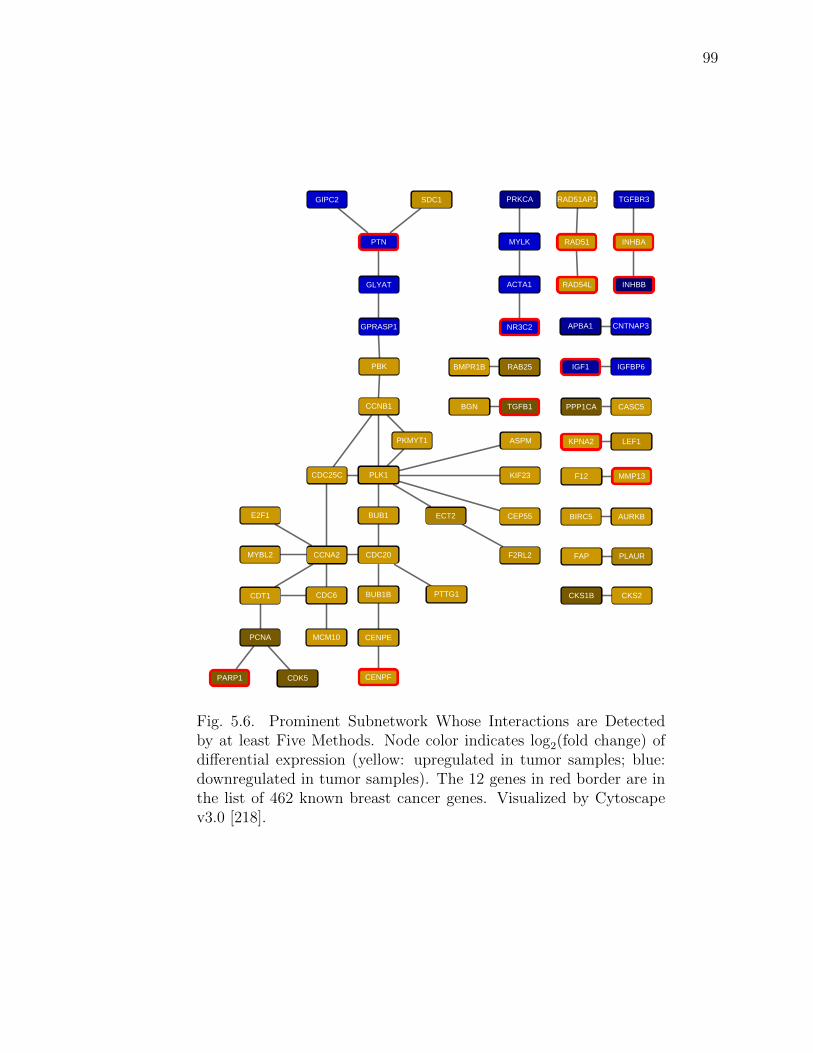
99

APBA1

RAD54L

NR3C2

INHBBACTA1

RAD51 INHBA

CNTNAP3

MYLK

CEP55ECT2

PLK1

CCNA2

CDC25C

MYBL2

BUB1

KIF23

E2F1

CDC20 F2RL2

PRKCASDC1GIPC2 RAD51AP1 TGFBR3

MCM10

CDK5

PTTG1

PCNA CENPE

BUB1BCDC6CDT1

PARP1 CENPF

AURKB

FAP

F12 MMP13

CKS1B

BIRC5

CKS2

PLAUR

CCNB1

PBK

GLYAT

GPRASP1

PTN

PKMYT1

RAB25

TGFB1

IGFBP6BMPR1B IGF1

PPP1CABGN CASC5

LEF1KPNA2ASPM

Fig. 5.6. Prominent Subnetwork Whose Interactions are Detectedby at least Five Methods. Node color indicates log2(fold change) ofdifferential expression (yellow: upregulated in tumor samples; blue:downregulated in tumor samples). The 12 genes in red border are inthe list of 462 known breast cancer genes. Visualized by Cytoscapev3.0 [218].

100

5.2 SysTox Challenge: Classification of Smoking Exposure

In this challenge, we are tasked to predict smoking exposure (smoker vs. non-

current smoker) or cessation (former smoker vs. never smoker) status using gene

expression data of human whole blood. The expression data, measured by microar-

rays, consist of 18, 604 genes in 224 samples for training and 1, 340 samples for testing.

Each samples are labeled as smoker, former smoker or never smoker. Generally, this

task can be considered as a classical classification problem in machine learning. We

employ three state-of-the-art classification methods to fulfill this task: Support Vec-

tor Machine (SVM), Random Forests (RF) and Artificial Neural Networks (ANN).

As a result, we report that SVM is the best performer again RF and ANN in two-fold

cross validation.

5.2.1 Introduction

Smoking is a primary risk factor for the development of various diseases, such as

lung cancer [225], Alzheimer’s disease [226], Parkinson’s disease [227], coronary heart

disease [228], inflammatory bowel disease [229], and so on. There are thousands

of chemicals in cigarettes. Some of those chemicals can enter the blood circulatory

system, which provides a way to monitor the smoking exposure of an individual

subject using gene expression of whole blood.

The whole challenge consists of two parts: sub-challenge 1 for human samples,

and sub-challenge 2 for mouse samples. In particular, sub-challenge 2 aims to verify

whether the human gene signatures derived in sub-challenge 1 can be used to predict

smoking exposure status in mouse samples. In this section, we report only the result

of sub-challenge 1 in predicting smoker

There are three given data sets, one for training and the other two for testing. All

the expression data are generated by microarrays consisting of 18, 604 human genes

and their expression in 224 training samples with labels, and 1, 340 testing samples

without labels (638 and 702 samples for round 1 and 2 tests, respectively). The

101

expression intensities are positive continuous values less than 20. We divided them

by 20 to scale them into [0, 1] before feeding them into the classifiers.

5.2.2 Methods: SVM, RF and ANN

Support vector machine, random forests and artificial neural networks are all

classical machine learning methods with many successful applications in various fields

of studies.

Support Vector Machines

Support vector machine (SVM) seeks a classification boundary with maximum

margin between different classes of objects. The boundary is, in fact, determined by

a set of support vectors (SVs), i.e., the set of objects closest to the boundary. This

makes SVM a robust classifier to outliers, since non-SV objects far away from the

boundary do not contribute to the determination of the boundary, and therefore do

not affect the final classification accuracy. For more complicated cases where two

classes of objects are not linear separable, SVM can adapt to these non-linear cases

by integrating various kernels in order to map the original feature space to a higher-

order separable space. The most complicated case is that the objects are still not

separable after being mapped to a high-order space using kernel trick. The current

standard version of SVM overcomes this challenge by introducing soft margin which

can tolerate a small portion of classification errors. This idea was proposed by Corinna

Cortes and Vladimir Vapnik in 1993 and was published in 1995 [230].

Random Forests

Random forest (RF) is an ensemble learning method that applies a voting strategy

to the classification results of many individual decision trees. It is simple to obtain

a satisfying and robust result using RF, since the only parameter to tune is the

102

number of trees. Normally, the more trees we grow, the better results we have.

Remarkably, RF is resistant to overfitting [231], which is an advantage compared to

neural networks, when the number of samples is much smaller than the number of

features. RF performs a bootstrap sampling from the training set to grow each tree,

which lowers the correlation among the trees and maximizes the forest diversity so as

to decrease overfitting. This advantage makes RF one of the most popular classifiers

in molecular diagnosis, since the number of patients is normally less than the number

of measured genes.

Artificial Neural Networks

Artificial Neural networks (ANN) and its extension, Deep learning, are a bioin-

spired model that mimics how brains recognize objects and memorize information. It

is a much more suitable approach for big data challenges than SVM and RF due to

its versatile infrastructure of hidden neurons. Its successful applications span various

fields of study in artificial intelligence, such as image classification, speech recogni-

tion, and recently, computer gaming (see AlphaGO [232]). Deep learning rebuilds

the fame of ANN by avoiding overfitting using advanced techniques such as max-

pooling (induction, [233]) and dropout (like amnesia, [234]). One of its extensions,

a deep convolution neural network (CNN) with 8 layers of neurons, trumped SVM

in image classification under the standard test using the largest image database, Im-

ageNET [235] with an error rate of 15.3% (CNN) compared to 26.2% (SVM) on

October 13, 2012. This is just the beginning of the deep learning era. However,

training a deep neural network is computationally expensive, since there are many

free parameters corresponding to the connections within and between the layers of

hidden neurons.

103

5.2.3 Results: Two-fold Cross Validation

We randomly split the given training samples into two sets, each of which consists

of 112 samples. Then we trained the three classifiers using one set and tested their

performances using the other, then we switched the two sets for a two-fold cross

validation.

For SVM, we downloaded LIBSVM, A Library for Support Vector Machines [236],

from the website: https://www.csie.ntu.edu.tw/~cjlin/libsvm/. This library

provides users with four different kernels: linear, polynomial, radial basis, and sig-

moid. We tested the performances of these four kernels using two-fold cross valida-

tions with 3 repeats. The result demonstrates that the linear kernel has the best

performance (Figure 5.7), since the feature space is already very high, and therefore

non-linear kernels contribute little to the prediction.

SVM Kernels

linear polynomial radial basis sigmoid

Pre

dic

tion E

rror

0

0.2

0.4

0.6

0.8

1

Fig. 5.7. Performances of SVMs with Different Kernels. The errorbars represent the standard deviations of prediction errors from 5repeats of cross-validation experiments.

For RF, we used the MATLAB built-in toolbox, TreeBagger to conduct the ex-

periment. More details about this toolbox can be found from the official website:

http://www.mathworks.com/help/stats/treebagger.html. We tested the perfor-

mances of RFs with different number of trees, 10, 100, and 1000, respectively, and

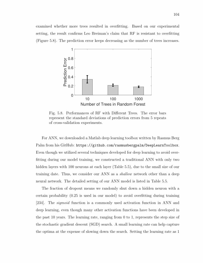
104

examined whether more trees resulted in overfitting. Based on our experimental

setting, the result confirms Leo Breiman’s claim that RF is resistant to overfitting

(Figure 5.8). The prediction error keeps decreasing as the number of trees increases.

Number of Trees in Random Forest

10 100 1000

Pre

dic

tio

n E

rro

r

0

0.2

0.4

0.6

0.8

1

Fig. 5.8. Performances of RF with Different Trees. The error barsrepresent the standard deviations of prediction errors from 5 repeatsof cross-validation experiments.

For ANN, we downloaded a Matlab deep learning toolbox written by Rasmus Berg

Palm from his GitHub: https://github.com/rasmusbergpalm/DeepLearnToolbox.

Even though we utilized several techniques developed for deep learning to avoid over-

fitting during our model training, we constructed a traditional ANN with only two

hidden layers with 100 neurons at each layer (Table 5.5), due to the small size of our

training date. Thus, we consider our ANN as a shallow network other than a deep

neural network. The detailed setting of our ANN model is listed in Table 5.5.

The fraction of dropout means we randomly shut down a hidden neuron with a

certain probability (0.25 is used in our model) to avoid overfitting during training

[234]. The sigmoid function is a commonly used activation function in ANN and

deep learning, even though many other activation functions have been developed in

the past 10 years. The learning rate, ranging from 0 to 1, represents the step size of

the stochastic gradient descent (SGD) search. A small learning rate can help capture

the optima at the expense of slowing down the search. Setting the learning rate as 1

105

Table 5.5Parameter Setting of ANN

ANN parameters Setting

Number of hidden layers 2

Number of neurons at each layer 100

Dropout fraction 0.25

Activation function sigmoid

Learning rate 1

Number of epochs 25

Batch size 35

in our model saves our computational time, but does not guarantee the training error

to reach the optima in our experiment (Figure 5.9). The number of epochs denotes

how many times the data propagate throughout the entire ANN during training. And

the batch size is a parameter of SGD indicating the sample size of a mini-batch over

which the gradient is averaged.

Figure 5.9 illustrates one of our training experiments using the parameter setting

listed in Table 5.5. The training error quickly reaches almost zero after 25 epochs.

However, a training error of zero in ANN does not guarantee an equally perfect error

rate in testing.

Taken together, we put the best performance of each method into Figure 5.10 for

comparison. We found that SVM with linear kernel is the best performer over RF

and ANN, with an averaged testing error of 12.65%. RF with 1000 trees has the

most stable performance with an averaged testing error of 17.86% and the smallest

standard deviation. ANN does not perform as well as SVM and RF due to overfitting

with an averaged testing error of 21.13%.

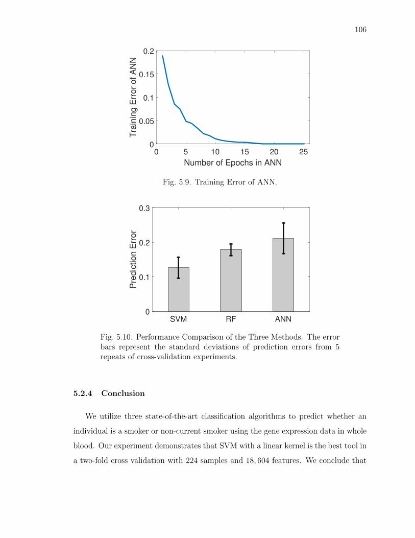
106

Number of Epochs in ANN

0 5 10 15 20 25

Tra

inin

g E

rror

of A

NN

0

0.05

0.1

0.15

0.2

Fig. 5.9. Training Error of ANN.

SVM RF ANN

Pre

dic

tio

n E

rro

r

0

0.1

0.2

0.3

Fig. 5.10. Performance Comparison of the Three Methods. The errorbars represent the standard deviations of prediction errors from 5repeats of cross-validation experiments.

5.2.4 Conclusion

We utilize three state-of-the-art classification algorithms to predict whether an

individual is a smoker or non-current smoker using the gene expression data in whole

blood. Our experiment demonstrates that SVM with a linear kernel is the best tool in

a two-fold cross validation with 224 samples and 18, 604 features. We conclude that

107

SVM and RF still have competitive performance in small data sets, whereas deep

learning requires large data sets to release its power.

Pick the right tool, a scissor or a mower.

108

6. SUMMARY

6.1 Discussion

In this thesis, I have developed three computational tools to label, partition,

and balance molecular networks, respectively. The results suggest that integrating

heterogeneous datasets into molecular networks can provide deeper insight into the

functional organization and behavior of biological molecules. Raw data of molecular

networks offer limited information for scientists to understand complex functional

behaviors. Those data show only which molecules directly interact with each other,

but they cannot be used to answer the following questions: (1) why are they con-

nected to each other, (2) how does the connection play a role in a complex biological

process, and (3) how does the connection change in different physiological conditions.

The success of AptRank in protein function prediction validates the hypothesis that

proteins with similar functions tend to interact with each other. BioSweeper reveals

the functional organization of molecule networks, and demonstrates how a team of

molecules performs a complex process by their connections. DifFBA uncovers con-

nections are not constant but dynamic, and these changes provide more insight in

understanding the molecular mechanism of phenotypic formation than the changes of

molecular quantities alone.

6.2 Future Direction

6.2.1 All-in-One: Differential Pathway Analysis (DiPAna)

In the future, I will incorporate the three models developed in this thesis, Ap-

tRank, BioSweeper and difFBA, into a unified model to perform Differential Path-

way Analysis (DiPAna) using quantitative proteomic data from complex diseases.

109

In particular, I will first use AptRank to obtain a “full” protein functional profile

given the incomplete functional annotations. Next, with the “full” functional profile,

BioSweeper will detect functionally enriched modules (protein complexes and path-

ways) which set up the boundaries of protein fluxes in a protein-protein interaction

network. Finally, I will generalize difFBA into a non-negative least squares model,

and solve it by robust regression algorithms to obtain a pathway-activity score for

each pathway. A differential analysis of this score between case and control samples

will indicate the extent to which a pathway is perturbed in diseased conditions, which

can highlight the pathways of interest for further pathological study. Interestingly,

dipana in Italian means disentangle, which fits the function of DiPAna: to disentangle

a molecular network into a dynamic modular diagram.

6.2.2 Perspective

In terms of biology, I believe that molecular networks are the language of molecular

function, but our current network models are still insufficient to explain complicated

biological processes. Integrating heterogeneous data is one of the most powerful

ways to enrich molecular networks. As more and more data on DNA methylation,

non-coding RNA expression, protein post-translational modification and metabolic

profiling become available, it will one day be feasible to construct a global molecular

map of an advanced organism. To come back to the ultimate question: why does one

molecule choose to interact with another? This question cannot be answered without

the light of evolution. Evolutionary game theory attempts to answer this kind of

question: why does one molecule decide to act cooperatively, and does the disruption

of this molecular cooperation lead to diseases. Are molecules selfish?

In terms of computer science, current advanced machine learning methods enable

automatic image classification, language translation, speech recognition and many

other complicated tasks. However, those techniques are still too young to understand

the world of biology. For example, using deep learning can successfully find a cat in

110

tons of images, or even videos. However, to identify causal genetic mutations from

genomic data to facilitate disease diagnosis is still a daunting challenge for current

artificial intelligence. Genomic medicine is becoming one of the most challenging

stages for scientists in artificial intelligence. And undoubtedly, finding an efficient

biomarker for disease diagnosis is more meaningful than finding a cat in videos.

LIST OF REFERENCES

111

LIST OF REFERENCES

[1] K.-I. Goh, M. E. Cusick, D. Valle, B. Childs, M. Vidal, and A.-L. Barabasi,“The human disease network,” Proceedings of the National Academy of Sciences,vol. 104, no. 21, pp. 8685–8690, 2007.

[2] M. A. Yıldırım, K.-I. Goh, M. E. Cusick, A.-L. Barabasi, and M. Vidal, “Drug-target network,” Nature Biotechnology, vol. 25, no. 10, pp. 1119–1126, 2007.

[3] G. W. Beadle and E. L. Tatum, “Genetic control of biochemical reactions inneurospora,” Proceedings of the National Academy of Sciences, vol. 27, no. 11,pp. 499–506, 1941.

[4] H. Kitano, “Biological robustness,” Nature Reviews Genetics, vol. 5, no. 11,pp. 826–837, 2004.

[5] M. Delbruck, “Unites biologiques douees de continuite genetique colloques in-ternationaux du centre national de la recherche scientifique,” Paris: CNRS,1949.

[6] M. Vidal, “A unifying view of 21st century systems biology,” FEBS letters,vol. 583, no. 24, pp. 3891–3894, 2009.

[7] C. Y. Logan and R. Nusse, “The Wnt signaling pathway in development anddisease,” Annual Review of Cell and Developmental Biology, vol. 20, pp. 781–810, 2004.

[8] J. D. Orth, I. Thiele, and B. Ø. Palsson, “What is flux balance analysis?,”Nature Biotechnology, vol. 28, no. 3, pp. 245–248, 2010.

[9] M. Watson, “Metabolic maps for the apple II,” Biochemical Society Transac-tions, vol. 12, no. 6, pp. 1093–1094, 1984.

[10] J. R. Karr, J. C. Sanghvi, D. N. Macklin, M. V. Gutschow, J. M. Jacobs,B. Bolival, N. Assad-Garcia, J. I. Glass, and M. W. Covert, “A whole-cellcomputational model predicts phenotype from genotype,” Cell, vol. 150, no. 2,pp. 389–401, 2012.

[11] N. J. Krogan, S. Lippman, D. A. Agard, A. Ashworth, and T. Ideker, “Thecancer cell map initiative: Defining the hallmark networks of cancer,” MolecularCell, vol. 58, no. 4, pp. 690–698, 2015.

[12] G. Ciriello, E. Cerami, C. Sander, and N. Schultz, “Mutual exclusivity anal-ysis identifies oncogenic network modules,” Genome Research, vol. 22, no. 2,pp. 398–406, 2012.

112

[13] J. Wang, H. Khiabanian, D. Rossi, G. Fabbri, V. Gattei, F. Forconi, L. Laurenti,R. Marasca, G. Del Poeta, R. Foa, L. Pasqualucci, G. Gaidano, and R. Rabadan,“Tumor evolutionary directed graphs and the history of chronic lymphocyticleukemia,” eLife, vol. 3, no. e02869, 2015.

[14] C. J. Ryan, P. Cimermancic, Z. A. Szpiech, A. Sali, R. D. Hernandez, and N. J.Krogan, “High-resolution network biology: connecting sequence with function,”Nature Reviews Genetics, vol. 14, no. 12, pp. 865–879, 2013.

[15] Q. Zhong, N. Simonis, Q.-R. Li, B. Charloteaux, F. Heuze, N. Klitgord, S. Tam,H. Yu, K. Venkatesan, D. Mou, V. Swearingen, M. A. Yildirim, H. Yan, A. Dri-cot, D. Szeto, C. Lin, T. Hao, C. Fan, S. Milstein, D. Dupuy, R. Brasseur, D. E.Hill, M. E. Cusick, and M. Vidal, “Edgetic perturbation models of human in-herited disorders,” Molecular Systems Biology, vol. 5, no. 321, 2009.

[16] T. Pawson and R. Linding, “Network medicine,” FEBS letters, vol. 582, no. 8,pp. 1266–1270, 2008.

[17] A.-L. Barabasi, N. Gulbahce, and J. Loscalzo, “Network medicine: a network-based approach to human disease,” Nature Reviews Genetics, vol. 12, no. 1,pp. 56–68, 2011.

[18] J. M. Irish, R. Hovland, P. O. Krutzik, O. D. Perez, Ø. Bruserud, B. T. Gjertsen,and G. P. Nolan, “Single cell profiling of potentiated phospho-protein networksin cancer cells,” Cell, vol. 118, no. 2, pp. 217–228, 2004.

[19] K. Komurov, J.-T. Tseng, M. Muller, E. G. Seviour, T. J. Moss, L. Yang, D. Na-grath, and P. T. Ram, “The glucose-deprivation network counteracts lapatinib-induced toxicity in resistant ErbB2-positive breast cancer cells,” Molecular Sys-tems Biology, vol. 8, no. 596, 2012.

[20] M. J. Lee, S. Y. Albert, A. K. Gardino, A. M. Heijink, P. K. Sorger,G. MacBeath, and M. B. Yaffe, “Sequential application of anticancer drugsenhances cell death by rewiring apoptotic signaling networks,” Cell, vol. 149,no. 4, pp. 780–794, 2012.

[21] R. Aebersold and M. Mann, “Mass spectrometry-based proteomics,” Nature,vol. 422, no. 6928, pp. 198–207, 2003.

[22] S.-E. Ong and M. Mann, “Mass spectrometry-based proteomics turns quanti-tative,” Nature Chemical Biology, vol. 1, no. 5, pp. 252–262, 2005.

[23] V. Lange, P. Picotti, B. Domon, and R. Aebersold, “Selected reaction monitor-ing for quantitative proteomics: a tutorial,” Molecular Systems Biology, vol. 4,no. 222, 2008.

[24] A. Maiolica, M. A. Junger, I. Ezkurdia, and R. Aebersold, “Targeted proteomeinvestigation via selected reaction monitoring mass spectrometry,” Journal ofProteomics, vol. 75, no. 12, pp. 3495–3513, 2012.

[25] P. Mallick and B. Kuster, “Proteomics: a pragmatic perspective,” NatureBiotechnology, vol. 28, no. 7, pp. 695–709, 2010.

[26] M.-S. Kim, S. M. Pinto, D. Getnet, R. S. Nirujogi, S. S. Manda, R. Chaerkady,A. K. Madugundu, D. S. Kelkar, R. Isserlin, S. Jain, et al., “A draft map of thehuman proteome,” Nature, vol. 509, no. 7502, pp. 575–581, 2014.

113

[27] M. Uhlen, L. Fagerberg, B. M. Hallstrom, C. Lindskog, P. Oksvold,A. Mardinoglu, A. Sivertsson, C. Kampf, E. Sjostedt, A. Asplund, I. Olsson,K. Edlund, E. Lundberg, S. Navani, C. A. Szigyarto, J. Odeberg, D. Djureinovic,J. O. Takanen, S. Hober, T. Alm, P. H. Edqvist, H. Berling, H. Tegel, J. Mul-der, J. Rockberg, P. Nilsson, J. M. Schwenk, M. Hamsten, K. von Feilitzen,M. Forsberg, L. Persson, F. Johansson, M. Zwahlen, G. von Heijne, J. Nielsen,and F. Ponten, “Tissue-based map of the human proteome,” Science, vol. 347,no. 6220, p. 394, 2015.

[28] J. Li, Y. Lu, R. Akbani, Z. Ju, P. L. Roebuck, W. Liu, J.-Y. Yang, B. M. Broom,R. G. Verhaak, D. W. Kane, C. Wakefield, J. N. Weinstein, G. B. Mills, andH. Liang, “TCPA: a resource for cancer functional proteomics data,” NatureMethods, vol. 10, no. 11, pp. 1046–1047, 2013.

[29] Z. Wang, M. Gerstein, and M. Snyder, “RNA-Seq: a revolutionary tool fortranscriptomics,” Nature Reviews Genetics, vol. 10, no. 1, pp. 57–63, 2009.

[30] T. Steijger, J. F. Abril, P. G. Engstrom, F. Kokocinski, T. J. Hubbard, R. Guigo,J. Harrow, P. Bertone, and RGASP Consortium, “Assessment of transcript re-construction methods for RNA-Seq,” Nature Methods, vol. 10, no. 12, pp. 1177–1184, 2013.

[31] N. L. Bray, H. Pimentel, P. Melsted, and L. Pachter, “Near-optimal probabilisticRNA-seq quantification,” Nature Biotechnology, vol. 34, no. 5, pp. 525–527,2016.

[32] R. Wang-Sattler, Z. Yu, C. Herder, A. C. Messias, A. Floegel, Y. He, K. Heim,M. Campillos, C. Holzapfel, B. Thorand, H. Grallert, T. Xu, E. Bader, C. Huth,K. Mittelstrass, A. Doring, C. Meisinger, C. Gieger, C. Prehn, W. Roemisch-Margl, M. Carstensen, L. Xie, H. Yamanaka-Okumura, G. Xing, U. Ceglarek,J. Thiery, G. Giani, H. Lickert, X. Lin, Y. Li, H. Boeing, H. G. Joost, M. H.de Angelis, W. Rathmann, K. Suhre, H. Prokisch, A. Peters, T. Meitinger,M. Roden, H. E. Wichmann, T. Pischon, J. Adamski, and T. Illig, “Novelbiomarkers for pre-diabetes identified by metabolomics,” Molecular SystemsBiology, vol. 8, no. 615, 2012.

[33] D. S. Wishart, D. Tzur, C. Knox, R. Eisner, A. C. Guo, N. Young, D. Cheng,K. Jewell, D. Arndt, S. Sawhney, C. Fung, L. Nikolai, M. Lewis, M. A. Coutouly,I. Forsythe, P. Tang, S. Shrivastava, K. Jeroncic, P. Stothard, G. Ameg-bey, D. Block, D. D. Hau, J. Wagner, J. Miniaci, M. Clements, M. Ge-bremedhin, N. Guo, Y. Zhang, G. E. Duggan, G. D. Macinnis, A. M. Weljie,R. Dowlatabadi, F. Bamforth, D. Clive, R. Greiner, L. Li, T. Marrie, B. D.Sykes, H. J. Vogel, and L. Querengesser, “HMDB: the human metabolomedatabase,” Nucleic Acids Research, vol. 35, no. suppl 1, pp. D521–D526, 2007.

114

[34] I. Thiele, N. Swainston, R. M. Fleming, A. Hoppe, S. Sahoo, M. K. Aurich,H. Haraldsdottir, M. L. Mo, O. Rolfsson, M. D. Stobbe, S. G. Thorleifsson,R. Agren, C. Bolling, S. Bordel, A. K. Chavali, P. Dobson, W. B. Dunn,L. Endler, D. Hala, M. Hucka, D. Hull, D. Jameson, N. Jamshidi, J. J. Jonsson,N. Juty, S. Keating, I. Nookaew, N. Le Novere, N. Malys, A. Mazein, J. A. Pa-pin, N. D. Price, E. Selkov, M. I. Sigurdsson, E. Simeonidis, N. Sonnenschein,K. Smallbone, A. Sorokin, J. H. van Beek, D. Weichart, I. Goryanin, J. Nielsen,H. V. Westerhoff, D. B. Kell, P. Mendes, and B. Ø. Palsson, “A community-driven global reconstruction of human metabolism,” Nature Biotechnology,vol. 31, no. 5, pp. 419–425, 2013.

[35] R. Chen, G. I. Mias, J. Li-Pook-Than, L. Jiang, H. Y. Lam, E. Miriami,K. J. Karczewski, M. Hariharan, F. E. Dewey, Y. Cheng, M. J. Clark, H. Im,L. Habegger, S. Balasubramanian, M. O’Huallachain, J. T. Dudley, S. Hillen-meyer, R. Haraksingh, D. Sharon, G. Euskirchen, P. Lacroute, K. Bettinger,A. P. Boyle, M. Kasowski, F. Grubert, S. Seki, M. Garcia, M. Whirl-Carrillo,M. Gallardo, M. A. Blasco, P. L. Greenberg, P. Snyder, T. E. Klein, R. B.Altman, A. J. Butte, E. A. Ashley, M. Gerstein, K. C. Nadeau, H. Tang, andM. Snyder, “Personal omics profiling reveals dynamic molecular and medicalphenotypes,” Cell, vol. 148, no. 6, pp. 1293–1307, 2012.

[36] S. Fields and O.-k. Song, “A novel genetic system to detect protein proteininteractions,” Nature, vol. 340, no. 6230, pp. 245–246, 1989.

[37] P. Uetz, L. Giot, G. Cagney, T. A. Mansfield, R. S. Judson, J. R. Knight,D. Lockshon, V. Narayan, M. Srinivasan, P. Pochart, A. Qureshi-Emili, Y. Li,B. Godwin, D. Conover, T. Kalbfleisch, G. Vijayadamodar, M. Yang, M. John-ston, S. Fields, and J. M. Rothberg, “A comprehensive analysis of protein–protein interactions in Saccharomyces cerevisiae,” Nature, vol. 403, no. 6770,pp. 623–627, 2000.

[38] A. J. Walhout, R. Sordella, X. Lu, J. L. Hartley, G. F. Temple, M. A. Brasch,N. Thierry-Mieg, and M. Vidal, “Protein interaction mapping in C. elegansusing proteins involved in vulval development,” Science, vol. 287, no. 5450,pp. 116–122, 2000.

[39] L. Giot, J. S. Bader, C. Brouwer, A. Chaudhuri, B. Kuang, Y. Li, Y. Hao,C. E. Ooi, B. Godwin, E. Vitols, G. Vijayadamodar, P. Pochart, H. Machineni,M. Welsh, Y. Kong, B. Zerhusen, R. Malcolm, Z. Varrone, A. Collis, M. Minto,S. Burgess, L. McDaniel, E. Stimpson, F. Spriggs, J. Williams, K. Neurath,N. Ioime, M. Agee, E. Voss, K. Furtak, R. Renzulli, N. Aanensen, S. Carrolla,E. Bickelhaupt, Y. Lazovatsky, A. DaSilva, J. Zhong, C. A. Stanyon, R. L. Fin-ley, K. P. White, M. Braverman, T. Jarvie, S. Gold, M. Leach, J. Knight, R. A.Shimkets, M. P. McKenna, J. Chant, and J. M. Rothberg, “A protein interactionmap of Drosophila melanogaster,” Science, vol. 302, no. 5651, pp. 1727–1736,2003.

115

[40] J.-F. Rual, K. Venkatesan, T. Hao, T. Hirozane-Kishikawa, A. Dricot, N. Li,G. F. Berriz, F. D. Gibbons, M. Dreze, N. Ayivi-Guedehoussou, N. Klitgord,C. Simon, M. Boxem, S. Milstein, J. Rosenberg, D. S. Goldberg, L. V. Zhang,S. L. Wong, G. Franklin, S. Li, J. S. Albala, J. Lim, C. Fraughton, E. Llamosas,S. Cevik, C. Bex, P. Lamesch, R. S. Sikorski, J. Vandenhaute, H. Y. Zoghbi,A. Smolyar, S. Bosak, R. Sequerra, L. Doucette-Stamm, M. E. Cusick, D. E.Hill, F. P. Roth, and M. Vidal, “Towards a proteome-scale map of the humanprotein–protein interaction network,” Nature, vol. 437, no. 7062, pp. 1173–1178,2005.

[41] H. Yu, P. Braun, M. A. Yıldırım, I. Lemmens, K. Venkatesan, J. Sahalie,T. Hirozane-Kishikawa, F. Gebreab, N. Li, N. Simonis, T. Hao, J. F. Rual,A. Dricot, A. Vazquez, R. R. Murray, C. Simon, L. Tardivo, S. Tam,N. Svrzikapa, C. Fan, A. S. de Smet, A. Motyl, M. E. Hudson, J. Park, X. Xin,M. E. Cusick, T. Moore, C. Boone, M. Snyder, F. P. Roth, A.-L. Barabasi,J. Tavernier, D. E. Hill, and M. Vidal, “High-quality binary protein interactionmap of the yeast interactome network,” Science, vol. 322, no. 5898, pp. 104–110,2008.

[42] S. V. Rajagopala, P. Sikorski, A. Kumar, R. Mosca, J. Vlasblom, R. Arnold,J. Franca-Koh, S. B. Pakala, S. Phanse, A. Ceol, R. Hauser, G. Siszler,S. Wuchty, A. Emili, M. Babu, P. Aloy, R. Pieper, and P. Uetz, “The binaryprotein-protein interaction landscape of Escherichia coli,” Nature Biotechnol-ogy, vol. 32, no. 3, pp. 285–290, 2014.

[43] T. Rolland, M. Tasan, B. Charloteaux, S. J. Pevzner, Q. Zhong, N. Sahni, S. Yi,I. Lemmens, C. Fontanillo, R. Mosca, A. Kamburov, S. D. Ghiassian, X. Yang,L. Ghamsari, D. Balcha, B. E. Begg, P. Braun, M. Brehme, M. P. Broly,A. R. Carvunis, D. Convery-Zupan, R. Corominas, J. Coulombe-Huntington,E. Dann, M. Dreze, A. Dricot, C. Fan, E. Franzosa, F. Gebreab, B. J. Gutierrez,M. F. Hardy, M. Jin, S. Kang, R. Kiros, G. N. Lin, K. Luck, A. MacWilliams,J. Menche, R. R. Murray, A. Palagi, M. M. Poulin, X. Rambout, J. Rasla,P. Reichert, V. Romero, E. Ruyssinck, J. M. Sahalie, A. Scholz, A. A. Shah,A. Sharma, Y. Shen, K. Spirohn, S. Tam, A. O. Tejeda, S. A. Trigg, J. C. Twiz-ere, K. Vega, J. Walsh, M. E. Cusick, Y. Xia, A.-L. Barabasi, L. M. Iakoucheva,P. Aloy, J. De Las Rivas, J. Tavernier, M. A. Calderwood, D. E. Hill, T. Hao,F. P. Roth, and M. Vidal, “A proteome-scale map of the human interactomenetwork,” Cell, vol. 159, no. 5, pp. 1212–1226, 2014.

[44] T. V. Vo, J. Das, M. J. Meyer, N. A. Cordero, N. Akturk, X. Wei, B. J. Fair,A. G. Degatano, R. Fragoza, L. G. Liu, A. Matsuyama, M. Trickey, S. Horibata,A. Grimson, H. Yamano, M. Yoshida, F. P. Roth, J. A. Pleiss, Y. Xia, andH. Yu, “A proteome-wide fission yeast interactome reveals network evolutionprinciples from yeasts to human,” Cell, vol. 164, no. 1-2, pp. 310–323, 2016.

[45] M. Vidal and S. Fields, “The yeast two-hybrid assay: still finding connectionsafter 25 years,” Nature Methods, vol. 11, no. 12, pp. 1203–1206, 2014.

[46] A.-C. Gingras, M. Gstaiger, B. Raught, and R. Aebersold, “Analysis of proteincomplexes using mass spectrometry,” Nature Reviews Molecular Cell Biology,vol. 8, no. 8, pp. 645–654, 2007.

116

[47] G. Rigaut, A. Shevchenko, B. Rutz, M. Wilm, M. Mann, and B. Seraphin, “Ageneric protein purification method for protein complex characterization andproteome exploration,” Nature Biotechnology, vol. 17, no. 10, pp. 1030–1032,1999.

[48] A.-C. Gavin, P. Aloy, P. Grandi, R. Krause, M. Boesche, M. Marzioch, C. Rau,L. J. Jensen, S. Bastuck, B. Dumpelfeld, A. Edelmann, M. A. Heurtier, V. Hoff-man, C. Hoefert, K. Klein, M. Hudak, A. M. Michon, M. Schelder, M. Schirle,M. Remor, T. Rudi, S. Hooper, A. Bauer, T. Bouwmeester, G. Casari,G. Drewes, G. Neubauer, J. M. Rick, B. Kuster, P. Bork, R. B. Russell, andG. Superti-Furga, “Proteome survey reveals modularity of the yeast cell ma-chinery,” Nature, vol. 440, no. 7084, pp. 631–636, 2006.

[49] N. J. Krogan, G. Cagney, H. Yu, G. Zhong, X. Guo, A. Ignatchenko, J. Li, S. Pu,N. Datta, A. P. Tikuisis, T. Punna, J. M. Peregrın-Alvarez, M. Shales, X. Zhang,M. Davey, M. D. Robinson, A. Paccanaro, J. E. Bray, A. Sheung, B. Beattie,D. P. Richards, V. Canadien, A. Lalev, F. Mena, P. Wong, A. Starostine, M. M.Canete, J. Vlasblom, S. Wu, C. Orsi, S. R. Collins, S. Chandran, R. Haw, J. J.Rilstone, K. Gandi, N. J. Thompson, G. Musso, P. St Onge, S. Ghanny, M. H.Lam, G. Butland, A. M. Altaf-Ul, S. Kanaya, A. Shilatifard, E. O’Shea, J. S.Weissman, C. J. Ingles, T. R. Hughes, J. Parkinson, M. Gerstein, S. J. Wodak,A. Emili, and J. F. Greenblatt, “Global landscape of protein complexes in theyeast Saccharomyces cerevisiae,” Nature, vol. 440, no. 7084, pp. 637–643, 2006.

[50] J. R. Hutchins, Y. Toyoda, B. Hegemann, I. Poser, J.-K. Heriche, M. M. Sykora,M. Augsburg, O. Hudecz, B. A. Buschhorn, J. Bulkescher, C. Conrad, D. Co-martin, A. Schleiffer, M. Sarov, A. Pozniakovsky, M. M. Slabicki, S. Schloiss-nig, I. Steinmacher, M. Leuschner, A. Ssykor, S. Lawo, L. Pelletier, H. Stark,K. Nasmyth, J. Ellenberg, R. Durbin, F. Buchholz, K. Mechtler, A. A. Hyman,and J. M. Peters, “Systematic analysis of human protein complexes identifieschromosome segregation proteins,” Science, vol. 328, no. 5978, pp. 593–599,2010.

[51] P. C. Havugimana, G. T. Hart, T. Nepusz, H. Yang, A. L. Turinsky, Z. Li, P. I.Wang, D. R. Boutz, V. Fong, S. Phanse, M. Babu, S. A. Craig, P. Hu, C. Wan,J. Vlasblom, V. U. Dar, A. Bezginov, G. W. Clark, G. C. Wu, S. J. Wodak,E. R. Tillier, A. Paccanaro, E. M. Marcotte, and A. Emili, “A census of humansoluble protein complexes,” Cell, vol. 150, no. 5, pp. 1068–1081, 2012.

[52] O. Rozenblatt-Rosen, R. C. Deo, M. Padi, G. Adelmant, M. A. Calderwood,T. Rolland, M. Grace, A. Dricot, M. Askenazi, M. Tavares, S. J. Pevzner,F. Abderazzaq, D. Byrdsong, A. R. Carvunis, A. A. Chen, J. Cheng, M. Cor-rell, M. Duarte, C. Fan, M. C. Feltkamp, S. B. Ficarro, R. Franchi, B. K. Garg,N. Gulbahce, T. Hao, A. M. Holthaus, R. James, A. Korkhin, L. Litovchick,J. C. Mar, T. R. Pak, S. Rabello, R. Rubio, Y. Shen, S. Singh, J. M. Spangle,M. Tasan, S. Wanamaker, J. T. Webber, J. Roecklein-Canfield, E. Johannsen,A.-L. Barabasi, R. Beroukhim, E. Kieff, M. E. Cusick, D. E. Hill, K. Munger,J. A. Marto, J. Quackenbush, F. P. Roth, J. A. DeCaprio, and M. Vidal, “Inter-preting cancer genomes using systematic host network perturbations by tumourvirus proteins,” Nature, vol. 487, no. 7408, pp. 491–495, 2012.

117

[53] A. Breitkreutz, H. Choi, J. R. Sharom, L. Boucher, V. Neduva, B. Larsen, Z.-Y.Lin, B.-J. Breitkreutz, C. Stark, G. Liu, J. Ahn, D. Dewar-Darch, T. Reguly,X. Tang, R. Almeida, Z. S. Qin, T. Pawson, A.-C. Gingras, A. I. Nesvizhskii,and M. Tyers, “A global protein kinase and phosphatase interaction network inyeast,” Science, vol. 328, no. 5981, pp. 1043–1046, 2010.

[54] A.-E. Saliba, I. Vonkova, S. Ceschia, G. M. Findlay, K. Maeda, C. Tischer,S. Deghou, V. van Noort, P. Bork, T. Pawson, J. Ellenberg, and A.-C. Gavin,“A quantitative liposome microarray to systematically characterize protein-lipidinteractions,” Nature Methods, vol. 11, no. 1, pp. 47–50, 2014.

[55] L. Gu, C. Li, J. Aach, D. E. Hill, M. Vidal, and G. M. Church, “Multiplex single-molecule interaction profiling of DNA-barcoded proteins,” Nature, vol. 515,no. 7528, pp. 554–557, 2014.

[56] D. S. Johnson, A. Mortazavi, R. M. Myers, and B. Wold, “Genome-wide map-ping of in vivo protein-DNA interactions,” Science, vol. 316, no. 5830, pp. 1497–1502, 2007.

[57] Q. C. Zhang, D. Petrey, L. Deng, L. Qiang, Y. Shi, C. A. Thu, B. Bisikirska,C. Lefebvre, D. Accili, T. Hunter, T. Maniatis, A. Califano, and B. Honig,“Structure-based prediction of protein-protein interactions on a genome-widescale,” Nature, vol. 490, no. 7421, pp. 556–560, 2012.

[58] D. La and D. Kihara, “A novel method for protein–protein interaction site pre-diction using phylogenetic substitution models,” Proteins: Structure, Function,and Bioinformatics, vol. 80, no. 1, pp. 126–141, 2012.

[59] M. Bansal, V. Belcastro, A. Ambesi-Impiombato, and D. Di Bernardo, “Howto infer gene networks from expression profiles,” Molecular Systems Biology,vol. 3, no. 78, 2007.

[60] M. B. Eisen, P. T. Spellman, P. O. Brown, and D. Botstein, “Cluster analysisand display of genome-wide expression patterns,” Proceedings of the NationalAcademy of Sciences, vol. 95, no. 25, pp. 14863–14868, 1998.

[61] B. Zhang and S. Horvath, “A general framework for weighted gene co-expressionnetwork analysis,” Statistical Applications in Genetics and Molecular Biology,vol. 4(1), no. 17, 2005.

[62] N. Friedman, M. Linial, I. Nachman, and D. Pe’er, “Using bayesian networksto analyze expression data,” Journal of Computational Biology, vol. 7, no. 3-4,pp. 601–620, 2000.

[63] A. J. Butte and I. S. Kohane, “Mutual information relevance networks: func-tional genomic clustering using pairwise entropy measurements,” in PacificSymposium on Biocomputing, vol. 5, pp. 418–429, 2000.

[64] P. D’haeseleer, X. Wen, S. Fuhrman, and R. Somogyi, “Linear modeling ofmRNA expression levels during CNS development and injury.,” in Pacific Sym-posium on Biocomputing, vol. 4, pp. 41–52, 1999.

[65] D. Marbach, J. C. Costello, R. Kuffner, N. M. Vega, R. J. Prill, D. M. Camacho,K. R. Allison, M. Kellis, J. J. Collins, G. Stolovitzky, and DREAM5 Consor-tium, “Wisdom of crowds for robust gene network inference,” Nature Methods,vol. 9, no. 8, pp. 796–804, 2012.

118

[66] C. Boone, H. Bussey, and B. J. Andrews, “Exploring genetic interactions andnetworks with yeast,” Nature Reviews Genetics, vol. 8, no. 6, pp. 437–449, 2007.

[67] A. H. Tong, M. Evangelista, A. B. Parsons, H. Xu, G. D. Bader, N. Page,M. Robinson, S. Raghibizadeh, C. W. Hogue, H. Bussey, B. Andrews, M. Tyers,and C. Boone, “Systematic genetic analysis with ordered arrays of yeast deletionmutants,” Science, vol. 294, no. 5550, pp. 2364–2368, 2001.

[68] A. H. Tong, G. Lesage, G. D. Bader, H. Ding, H. Xu, X. Xin, J. Young, G. F.Berriz, R. L. Brost, M. Chang, Y. Chen, X. Cheng, G. Chua, H. Friesen, D. S.Goldberg, J. Haynes, C. Humphries, G. He, S. Hussein, L. Ke, N. Krogan,Z. Li, J. N. Levinson, H. Lu, P. Menard, C. Munyana, A. B. Parsons, O. Ryan,R. Tonikian, T. Roberts, A. M. Sdicu, J. Shapiro, B. Sheikh, B. Suter, S. L.Wong, L. V. Zhang, H. Zhu, C. G. Burd, S. Munro, C. Sander, J. Rine, J. Green-blatt, M. Peter, A. Bretscher, G. Bell, F. P. Roth, G. W. Brown, B. Andrews,H. Bussey, and C. Boone, “Global mapping of the yeast genetic interactionnetwork,” Science, vol. 303, no. 5659, pp. 808–813, 2004.

[69] M. Costanzo, A. Baryshnikova, J. Bellay, Y. Kim, E. D. Spear, C. S. Sevier,H. Ding, J. L. Koh, K. Toufighi, S. Mostafavi, J. Prinz, R. P. St Onge, B. Van-derSluis, T. Makhnevych, F. J. Vizeacoumar, S. Alizadeh, S. Bahr, R. L. Brost,Y. Chen, M. Cokol, R. Deshpande, Z. Li, Z. Y. Lin, W. Liang, M. Marback,J. Paw, B. J. San Luis, E. Shuteriqi, A. H. Tong, N. van Dyk, I. M. Wallace,J. A. Whitney, M. T. Weirauch, G. Zhong, H. Zhu, W. A. Houry, M. Brudno,S. Ragibizadeh, B. Papp, C. Pal, F. P. Roth, G. Giaever, C. Nislow, O. G. Troy-anskaya, H. Bussey, G. D. Bader, A.-C. Gingras, Q. D. Morris, P. M. Kim, C. A.Kaiser, C. L. Myers, B. J. Andrews, and C. Boone, “The genetic landscape ofa cell,” Science, vol. 327, no. 5964, pp. 425–431, 2010.

[70] S. Bandyopadhyay, M. Mehta, D. Kuo, M. K. Sung, R. Chuang, E. J. Jaehnig,B. Bodenmiller, K. Licon, W. Copeland, M. Shales, D. Fiedler, J. Dutkowski,A. Guenole, H. van Attikum, K. M. Shokat, R. D. Kolodner, W. K. Huh,R. Aebersold, M. C. Keogh, N. J. Krogan, and T. Ideker, “Rewiring of geneticnetworks in response to DNA damage,” Science, vol. 330, no. 6009, pp. 1385–1389, 2010.

[71] A. Roguev, D. Talbot, G. L. Negri, M. Shales, G. Cagney, S. Bandyopadhyay,B. Panning, and N. J. Krogan, “Quantitative genetic-interaction mapping inmammalian cells,” Nature Methods, vol. 10, no. 5, pp. 432–437, 2013.

[72] P. Erdos and A. Renyi, “On random graphs,” Publicationes Mathematicae De-brecen, vol. 6, pp. 290–297, 1959.

[73] A.-L. Barabasi and R. Albert, “Emergence of scaling in random networks,”Science, vol. 286, no. 5439, pp. 509–512, 1999.

[74] M. P. Stumpf, C. Wiuf, and R. M. May, “Subnets of scale-free networks arenot scale-free: sampling properties of networks,” Proceedings of the NationalAcademy of Sciences, vol. 102, no. 12, pp. 4221–4224, 2005.

[75] R. Khanin and E. Wit, “How scale-free are biological networks,” Journal ofComputational Biology, vol. 13, no. 3, pp. 810–818, 2006.

[76] H. Jeong, S. P. Mason, A.-L. Barabasi, and Z. N. Oltvai, “Lethality and cen-trality in protein networks,” Nature, vol. 411, no. 6833, pp. 41–42, 2001.

119

[77] J.-D. J. Han, N. Bertin, T. Hao, D. S. Goldberg, G. F. Berriz, L. V. Zhang,D. Dupuy, A. J. Walhout, M. E. Cusick, F. P. Roth, and M. Vidal, “Evidencefor dynamically organized modularity in the yeast protein-protein interactionnetwork,” Nature, vol. 430, no. 6995, pp. 88–93, 2004.

[78] I. W. Taylor, R. Linding, D. Warde-Farley, Y. Liu, C. Pesquita, D. Faria, S. Bull,T. Pawson, Q. Morris, and J. L. Wrana, “Dynamic modularity in protein inter-action networks predicts breast cancer outcome,” Nature Biotechnology, vol. 27,no. 2, pp. 199–204, 2009.

[79] E. W. Dijkstra, “A note on two problems in connexion with graphs,” Nu-merische mathematik, vol. 1, no. 1, pp. 269–271, 1959.

[80] R. Bellman, “On the theory of dynamic programming,” Proceedings of the Na-tional Academy of Sciences, vol. 38, no. 8, pp. 716–719, 1952.

[81] S. Milgram, “The small world problem,” Psychology Today, vol. 1, no. 1, pp. 60–67, 1967.

[82] J. Guare, Six degrees of separation: A play. Vintage Books, New York, 1990.

[83] D. J. Watts and S. H. Strogatz, “Collective dynamics of “small-world” net-works,” Nature, vol. 393, no. 6684, pp. 440–442, 1998.

[84] Q. K. Telesford, K. E. Joyce, S. Hayasaka, J. H. Burdette, and P. J. Lauri-enti, “The ubiquity of small-world networks,” Brain Connectivity, vol. 1, no. 5,pp. 367–375, 2011.

[85] L. C. Freeman, “A set of measures of centrality based on betweenness,” So-ciometry, pp. 35–41, 1977.

[86] H. Yu, P. M. Kim, E. Sprecher, V. Trifonov, and M. Gerstein, “The impor-tance of bottlenecks in protein networks: correlation with gene essentiality andexpression dynamics,” PLoS Computational Biology, vol. 3, no. 4, p. e59, 2007.

[87] R. D. Luce and A. D. Perry, “A method of matrix analysis of group structure,”Psychometrika, vol. 14, no. 2, pp. 95–116, 1949.

[88] L. H. Hartwell, J. J. Hopfield, S. Leibler, and A. W. Murray, “From molecularto modular cell biology,” Nature, vol. 402, pp. C47–C52, 1999.

[89] E. Ravasz, A. L. Somera, D. A. Mongru, Z. N. Oltvai, and A.-L. Barabasi, “Hi-erarchical organization of modularity in metabolic networks,” Science, vol. 297,no. 5586, pp. 1551–1555, 2002.

[90] M. Girvan and M. E. Newman, “Community structure in social and biologicalnetworks,” Proceedings of the National Academy of Sciences, vol. 99, no. 12,pp. 7821–7826, 2002.

[91] M. E. Newman and M. Girvan, “Finding and evaluating community structurein networks,” Physical Review E, vol. 69, no. 2, p. 026113, 2004.

[92] M. E. Newman, “Modularity and community structure in networks,” Proceed-ings of the National Academy of Sciences, vol. 103, no. 23, pp. 8577–8582, 2006.

120

[93] S. Fortunato, “Community detection in graphs,” Physics Reports, vol. 486,no. 3, pp. 75–174, 2010.

[94] T. Ideker and N. J. Krogan, “Differential network biology,” Molecular SystemsBiology, vol. 8, no. 565, 2012.

[95] M. Dreze, B. Charloteaux, S. Milstein, P.-O. Vidalain, M. A. Yildirim,Q. Zhong, N. Svrzikapa, V. Romero, G. Laloux, R. Brasseur, J. Vandenhaute,M. Boxem, M. E. Cusick, D. E. Hill, and M. Vidal, ““Edgetic” perturbationof a C. elegans BCL2 ortholog,” Nature Methods, vol. 6, no. 11, pp. 843–849,2009.

[96] X. Wang, X. Wei, B. Thijssen, J. Das, S. M. Lipkin, and H. Yu, “Three-dimensional reconstruction of protein networks provides insight into humangenetic disease,” Nature Biotechnology, vol. 30, no. 2, pp. 159–164, 2012.

[97] N. Sahni, S. Yi, M. Taipale, J. I. F. Bass, J. Coulombe-Huntington, F. Yang,J. Peng, J. Weile, G. I. Karras, Y. Wang, I. A. Kovacs, A. Kamburov, I. Kryk-baeva, M. H. Lam, G. Tucker, V. Khurana, A. Sharma, Y. Y. Liu, N. Yachie,Q. Zhong, Y. Shen, A. Palagi, A. San-Miguel, C. Fan, D. Balcha, A. Dricot,D. M. Jordan, J. M. Walsh, A. A. Shah, X. Yang, A. K. Stoyanova, A. Leighton,M. A. Calderwood, Y. Jacob, M. E. Cusick, K. Salehi-Ashtiani, L. J. Whitesell,S. Sunyaev, B. Berger, A.-L. Barabasi, B. Charloteaux, D. E. Hill, T. Hao, F. P.Roth, Y. Xia, A. J. Walhout, S. Lindquist, and M. Vidal, “Widespread macro-molecular interaction perturbations in human genetic disorders,” Cell, vol. 161,no. 3, pp. 647–660, 2015.

[98] X. Yang, J. Coulombe-Huntington, S. Kang, G. M. Sheynkman, T. Hao,A. Richardson, S. Sun, F. Yang, Y. A. Shen, R. R. Murray, K. Spirohn, B. E.Begg, M. Duran-Frigola, A. MacWilliams, S. J. Pevzner, Q. Zhong, S. A. Trigg,S. Tam, L. Ghamsari, N. Sahni, S. Yi, M. D. Rodriguez, D. Balcha, G. Tan,M. Costanzo, B. Andrews, C. Boone, X. J. Zhou, K. Salehi-Ashtiani, B. Char-loteaux, A. A. Chen, M. A. Calderwood, P. Aloy, F. P. Roth, D. E. Hill, L. M.Iakoucheva, Y. Xia, and M. Vidal, “Widespread expansion of protein interactioncapabilities by alternative splicing,” Cell, vol. 164, no. 4, pp. 805–817, 2016.

[99] N. Sahni, S. Yi, Q. Zhong, N. Jailkhani, B. Charloteaux, M. E. Cusick, andM. Vidal, “Edgotype: a fundamental link between genotype and phenotype,”Current Opinion in Genetics and Development, vol. 23, no. 6, pp. 649–657,2013.

[100] P. Creixell, A. Palmeri, C. J. Miller, H. J. Lou, C. C. Santini, M. Nielsen, B. E.Turk, and R. Linding, “Unmasking determinants of specificity in the humankinome,” Cell, vol. 163, no. 1, pp. 187–201, 2015.

[101] P. Creixell, E. M. Schoof, C. D. Simpson, J. Longden, C. J. Miller, H. J. Lou,L. Perryman, T. R. Cox, N. Zivanovic, A. Palmeri, A. Wesolowska-Andersen,M. Helmer-Citterich, J. Ferkinghoff-Borg, H. Itamochi, B. Bodenmiller, J. T.Erler, B. E. Turk, and R. Linding, “Kinome-wide decoding of network-attackingmutations rewiring cancer signaling,” Cell, vol. 163, no. 1, pp. 202–217, 2015.

[102] M. AlQuraishi, G. Koytiger, A. Jenney, G. MacBeath, and P. K. Sorger, “Amultiscale statistical mechanical framework integrates biophysical and genomicdata to assemble cancer networks,” Nature Genetics, vol. 46, no. 12, pp. 1363–1371, 2014.

121

[103] N. Bisson, D. A. James, G. Ivosev, S. A. Tate, R. Bonner, L. Taylor, andT. Pawson, “Selected reaction monitoring mass spectrometry reveals the dy-namics of signaling through the grb2 adaptor,” Nature Biotechnology, vol. 29,no. 7, pp. 653–658, 2011.

[104] B. C. Collins, L. C. Gillet, G. Rosenberger, H. L. Rost, A. Vichalkovski,M. Gstaiger, and R. Aebersold, “Quantifying protein interaction dynamics byswath mass spectrometry: application to the 14-3-3 system,” Nature Methods,vol. 10, no. 12, pp. 1246–1253, 2013.

[105] J.-P. Lambert, G. Ivosev, A. L. Couzens, B. Larsen, M. Taipale, Z.-Y. Lin,Q. Zhong, S. Lindquist, M. Vidal, R. Aebersold, T. Pawson, R. Bonner, S. Tate,and A.-C. Gingras, “Mapping differential interactomes by affinity purificationcoupled with data-independent mass spectrometry acquisition,” Nature Meth-ods, vol. 10, no. 12, pp. 1239–1245, 2013.

[106] S. Krishnaswamy, M. H. Spitzer, M. Mingueneau, S. C. Bendall, O. Litvin,E. Stone, D. Pe’er, and G. P. Nolan, “Conditional density-based analysis of Tcell signaling in single-cell data,” Science, vol. 346, no. 6213, p. 1250689, 2014.

[107] L. Pena-Castillo, M. Tasan, C. L. Myers, H. Lee, T. Joshi, C. Zhang, Y. Guan,M. Leone, A. Pagnani, W. K. Kim, C. Krumpelman, W. Tian, G. Obozinski,Y. Qi, S. Mostafavi, G. N. Lin, G. F. Berriz, F. D. Gibbons, G. Lanckriet, J. Qiu,C. Grant, Z. Barutcuoglu, D. P. Hill, D. Warde-Farley, C. Grouios, D. Ray, J. A.Blake, M. Deng, M. I. Jordan, W. S. Noble, Q. Morris, J. Klein-Seetharaman,Z. Bar-Joseph, T. Chen, F. Sun, O. G. Troyanskaya, E. M. Marcotte, D. Xu,T. R. Hughes, and F. P. Roth, “A critical assessment of Mus musculus genefunction prediction using integrated genomic evidence,” Genome Biology, vol. 9,no. S2, 2008.

[108] P. Radivojac, W. T. Clark, T. R. Oron, A. M. Schnoes, T. Wittkop, A. Sokolov,K. Graim, C. Funk, K. Verspoor, A. Ben-Hur, G. Pandey, J. M. Yunes, A. S.Talwalkar, S. Repo, M. L. Souza, D. Piovesan, R. Casadio, Z. Wang, J. Cheng,H. Fang, J. Gough, P. Koskinen, P. Toronen, J. Nokso-Koivisto, L. Holm,D. Cozzetto, D. W. Buchan, K. Bryson, D. T. Jones, B. Limaye, H. Inam-dar, A. Datta, S. K. Manjari, R. Joshi, M. Chitale, D. Kihara, A. M. Lisewski,S. Erdin, E. Venner, O. Lichtarge, R. Rentzsch, H. Yang, A. E. Romero, P. Bhat,A. Paccanaro, T. Hamp, R. Kaßner, S. Seemayer, E. Vicedo, C. Schaefer,D. Achten, F. Auer, A. Boehm, T. Braun, M. Hecht, M. Heron, P. Honigschmid,T. A. Hopf, S. Kaufmann, M. Kiening, D. Krompass, C. Landerer, Y. Mahlich,M. Roos, J. Bjorne, T. Salakoski, A. Wong, H. Shatkay, F. Gatzmann, I. Som-mer, M. N. Wass, M. J. Sternberg, N. Skunca, F. Supek, M. Bosnjak, P. Panov,S. Dzeroski, T. Smuc, Y. A. Kourmpetis, A. D. van Dijk, C. J. ter Braak,Y. Zhou, Q. Gong, X. Dong, W. Tian, M. Falda, P. Fontana, E. Lavezzo,B. Di Camillo, S. Toppo, L. Lan, N. Djuric, Y. Guo, S. Vucetic, A. Bairoch,M. Linial, P. C. Babbitt, S. E. Brenner, C. Orengo, B. Rost, S. D. Mooney, andF. I., “A large-scale evaluation of computational protein function prediction,”Nature Methods, vol. 10, no. 3, pp. 221–227, 2013.

[109] S. Mostafavi, D. Ray, D. Warde-Farley, C. Grouios, and Q. Morris, “GeneMA-NIA: a real-time multiple association network integration algorithm for predict-ing gene function,” Genome Biology, vol. 9, no. S4, 2008.

122

[110] R. Sharan, I. Ulitsky, and R. Shamir, “Network-based prediction of proteinfunction,” Molecular Systems Biology, vol. 3, no. 88, 2007.

[111] B. Schwikowski, P. Uetz, and S. Fields, “A network of protein–protein interac-tions in yeast,” Nature Biotechnology, vol. 18, no. 12, pp. 1257–1261, 2000.

[112] A. J. Enright, S. Van Dongen, and C. A. Ouzounis, “An efficient algorithm forlarge-scale detection of protein families,” Nucleic Acids Research, vol. 30, no. 7,pp. 1575–1584, 2002.

[113] G. D. Bader and C. W. Hogue, “An automated method for finding molecularcomplexes in large protein interaction networks,” BMC Bioinformatics, vol. 4,no. 2, 2003.

[114] E. Nabieva, K. Jim, A. Agarwal, B. Chazelle, and M. Singh, “Whole-proteomeprediction of protein function via graph-theoretic analysis of interaction maps,”Bioinformatics, vol. 21, no. suppl 1, pp. i302–i310, 2005.

[115] L. Page, S. Brin, R. Motwani, and T. Winograd, “The PageRank citation rank-ing: bringing order to the web.,” Technical Report, Stanford University, Stan-ford, CA, no. 1999-66, 1999.

[116] V. Freschi, “Protein function prediction from interaction networks using a ran-dom walk ranking algorithm,” in Proceedings of the 7th IEEE InternationalConference on Bioinformatics and Bioengineering, pp. 42–48, IEEE, 2007.

[117] D. Zhou, O. Bousquet, T. N. Lal, J. Weston, and B. Scholkopf, “Learningwith local and global consistency,” Advances in Neural Information ProcessingSystems, vol. 16, no. 16, pp. 321–328, 2004.

[118] G. Yu, H. Rangwala, C. Domeniconi, G. Zhang, and Z. Yu, “Protein functionprediction using multi-label ensemble classification,” IEEE/ACM Transactionson Computational Biology and Bioinformatics, vol. 10, no. 4, pp. 1–1, 2013.

[119] H. Wang, H. Huang, and C. Ding, “Image annotation using bi-relational graphof images and semantic labels,” in IEEE Conference on Computer Vision andPattern Recognition, pp. 793–800, IEEE, 2011.

[120] Gene Ontology Consortium, “The Gene Ontology (GO) database and infor-matics resource,” Nucleic Acids Research, vol. 32, no. suppl 1, pp. D258–D261,2004.

[121] O. D. King, R. E. Foulger, S. S. Dwight, J. V. White, and F. P. Roth, “Pre-dicting gene function from patterns of annotation,” Genome Research, vol. 13,no. 5, pp. 896–904, 2003.

[122] Z. Barutcuoglu, R. E. Schapire, and O. G. Troyanskaya, “Hierarchical multi-label prediction of gene function,” Bioinformatics, vol. 22, no. 7, pp. 830–836,2006.

[123] G. Valentini, “True path rule hierarchical ensembles for genome-wide genefunction prediction,” IEEE/ACM Transactions on Computational Biology andBioinformatics, vol. 8, no. 3, pp. 832–847, 2011.

123

[124] G. Valentini, “Hierarchical ensemble methods for protein function prediction,”International Scholarly Research Notices Bioinformatics, vol. 2014, no. 901419,2014.

[125] Y. Tao, L. Sam, J. Li, C. Friedman, and Y. A. Lussier, “Information theoryapplied to the sparse gene ontology annotation network to predict novel genefunction,” Bioinformatics, vol. 23, no. 13, pp. i529–i538, 2007.

[126] G. Pandey, C. L. Myers, and V. Kumar, “Incorporating functional inter-relationships into protein function prediction algorithms,” BMC Bioinformatics,vol. 10, no. 142, 2009.

[127] D. Lin, “An information-theoretic definition of similarity,” in International Con-ference on Machine Learning, vol. 98, pp. 296–304, 1998.

[128] A. Sokolov and A. Ben-Hur, “Hierarchical classification of gene ontology termsusing the gostruct method,” Journal of Bioinformatics and Computational Bi-ology, vol. 8, no. 02, pp. 357–376, 2010.

[129] I. Tsochantaridis, T. Joachims, T. Hofmann, and Y. Altun, “Large marginmethods for structured and interdependent output variables,” in Journal ofMachine Learning Research, pp. 1453–1484, 2005.

[130] G. Yu, H. Zhu, C. Domeniconi, and J. Liu, “Predicting protein function viadownward random walks on a gene ontology,” BMC Bioinformatics, vol. 16,no. 271, 2015.

[131] S. Wang, H. Cho, C. Zhai, B. Berger, and J. Peng, “Exploiting ontology graphfor predicting sparsely annotated gene function,” Bioinformatics, vol. 31, no. 12,pp. i357–i364, 2015.

[132] J. Gillis and P. Pavlidis, “The impact of multifunctional genes on “guilt byassociation” analysis,” PLoS One, vol. 6(2), no. e17258, 2011.

[133] J. Gillis and P. Pavlidis, ““Guilt by association” is the exception rather thanthe rule in gene networks,” PLoS Computational Biology, vol. 8, no. 3, 2012.

[134] P. Pavlidis and J. Gillis, “Progress and challenges in the computational pre-diction of gene function using networks: 2012-2013 update,” F1000Research,vol. 2, no. 230, 2013.

[135] J. Gillis, S. Ballouz, and P. Pavlidis, “Bias tradeoffs in the creation and anal-ysis of protein–protein interaction networks,” Journal of Proteomics, vol. 100,pp. 44–54, 2014.

[136] Gene Ontology Consortium, “Gene Ontology Consortium: going forward,” Nu-cleic acids research, vol. 43, no. D1, pp. D1049–D1056, 2015.

[137] H. Tong, “Fast random walk with restart and its applications,” in Proceedingsof the 6th IEEE International Conference on Data Mining, 2006.

[138] G. Jeh and J. Widom, “Scaling personalized web search,” in Proceedings of the12th international Conference on the World Wide Web, pp. 271–279, ACM,2003.

124

[139] R. Baeza-Yates, P. Boldi, and C. Castillo, “Generalizing PageRank: Dampingfunctions for link-based ranking algorithms,” in Proceedings of the 29th An-nual International ACM SIGIR Conference on Research and Development inInformation Retrieval, pp. 308–315, ACM, 2006.

[140] P. G. Constantine and D. F. Gleich, “Random alpha PageRank,” Internet Math-ematics, vol. 6, no. 2, pp. 189–236, 2010.

[141] F. Chung, “The heat kernel as the PageRank of a graph,” Proceedings of theNational Academy of Sciences, vol. 104, no. 50, pp. 19735–19740, 2007.

[142] X. Zhu, W. Nejdl, and M. Georgescu, “An adaptive teleportation random walkmodel for learning social tag relevance,” in Proceedings of the 37th Interna-tional ACM SIGIR Conference on Research and Development in InformationRetrieval, pp. 223–232, ACM, 2014.

[143] S. Mostafavi and Q. Morris, “Fast integration of heterogeneous data sourcesfor predicting gene function with limited annotation,” Bioinformatics, vol. 26,no. 14, pp. 1759–1765, 2010.

[144] H. Cho, B. Berger, and J. Peng, “Diffusion component analysis: unraveling func-tional topology in biological networks,” in Research in Computational MolecularBiology, pp. 62–64, Springer, 2015.

[145] C. Stark, B.-J. Breitkreutz, T. Reguly, L. Boucher, A. Breitkreutz, and M. Ty-ers, “BioGRID: a general repository for interaction datasets,” Nucleic AcidsResearch, vol. 34, no. suppl 1, pp. D535–D539, 2006.

[146] W. Verleyen, S. Ballouz, and J. Gillis, “Positive and negative forms of replica-bility in gene network analysis,” Bioinformatics, vol. 32, no. 7, pp. 1065–1073,2015.

[147] K. Mitra, A.-R. Carvunis, S. K. Ramesh, and T. Ideker, “Integrative approachesfor finding modular structure in biological networks,” Nature Reviews Genetics,vol. 14, no. 10, pp. 719–732, 2013.

[148] N. Przulj, D. A. Wigle, and I. Jurisica, “Functional topology in a network ofprotein interactions,” Bioinformatics, vol. 20, no. 3, pp. 340–348, 2004.

[149] G. Palla, I. Derenyi, I. Farkas, and T. Vicsek, “Uncovering the overlapping com-munity structure of complex networks in nature and society,” Nature, vol. 435,no. 7043, pp. 814–818, 2005.

[150] B. Adamcsek, G. Palla, I. J. Farkas, I. Derenyi, and T. Vicsek, “CFinder: lo-cating cliques and overlapping modules in biological networks,” Bioinformatics,vol. 22, no. 8, pp. 1021–1023, 2006.

[151] B. J. Frey and D. Dueck, “Clustering by passing messages between data points,”Science, vol. 315, no. 5814, pp. 972–976, 2007.

[152] K. Macropol, T. Can, and A. K. Singh, “RRW: repeated random walks ongenome-scale protein networks for local cluster discovery,” BMC Bioinformat-ics, vol. 10, no. 283, 2009.

125

[153] Y.-Y. Ahn, J. P. Bagrow, and S. Lehmann, “Link communities reveal multiscalecomplexity in networks,” Nature, vol. 466, no. 7307, pp. 761–764, 2010.

[154] A. T. Kalinka and P. Tomancak, “Linkcomm: an R package for the generation,visualization, and analysis of link communities in networks of arbitrary size andtype,” Bioinformatics, vol. 27, no. 14, pp. 2011–2012, 2011.

[155] T. Nepusz, H. Yu, and A. Paccanaro, “Detecting overlapping protein complexesin protein-protein interaction networks,” Nature Methods, vol. 9, no. 5, pp. 471–472, 2012.

[156] C. Wiwie, J. Baumbach, and R. Rottger, “Comparing the performance ofbiomedical clustering methods,” Nature methods, vol. 12, no. 11, pp. 1033–1038,2015.

[157] Z. Lubovac, J. Gamalielsson, and B. Olsson, “Combining functional and topo-logical properties to identify core modules in protein interaction networks,”Proteins: Structure, Function, and Bioinformatics, vol. 64, no. 4, pp. 948–959,2006.

[158] Y.-R. Cho, W. Hwang, M. Ramanathan, and A. Zhang, “Semantic integrationto identify overlapping functional modules in protein interaction networks,”BMC Bioinformatics, vol. 8, no. 265, 2007.

[159] M. T. Dittrich, G. W. Klau, A. Rosenwald, T. Dandekar, and T. Muller, “Identi-fying functional modules in protein–protein interaction networks: an integratedexact approach,” Bioinformatics, vol. 24, no. 13, pp. i223–i231, 2008.

[160] D. Boyanova, S. Nilla, G. W. Klau, T. Dandekar, T. Muller, and M. Dittrich,“Functional module search in protein networks based on semantic similarityimproves the analysis of proteomics data,” Molecular and Cellular Proteomics,vol. 13, no. 7, pp. 1877–1889, 2014.

[161] C. M. Taniguchi, B. Emanuelli, and C. R. Kahn, “Critical nodes in signallingpathways: insights into insulin action,” Nature Reviews Molecular Cell Biology,vol. 7, no. 2, pp. 85–96, 2006.

[162] P. J. Mucha, T. Richardson, K. Macon, M. A. Porter, and J.-P. Onnela, “Com-munity structure in time-dependent, multiscale, and multiplex networks,” Sci-ence, vol. 328, no. 5980, pp. 876–878, 2010.

[163] S. Zhang, Q. Li, J. Liu, and X. J. Zhou, “A novel computational frame-work for simultaneous integration of multiple types of genomic data to identifymicroRNA-gene regulatory modules,” Bioinformatics, vol. 27, no. 13, pp. i401–i409, 2011.

[164] W. Li, S. Zhang, C.-C. Liu, and X. J. Zhou, “Identifying multi-layer gene regu-latory modules from multi-dimensional genomic data,” Bioinformatics, vol. 28,no. 19, pp. 2458–2466, 2012.

[165] B. Wang, A. M. Mezlini, F. Demir, M. Fiume, Z. Tu, M. Brudno, B. Haibe-Kains, and A. Goldenberg, “Similarity network fusion for aggregating data typeson a genomic scale,” Nature Methods, vol. 11, no. 3, pp. 333–337, 2014.

126

[166] D. F. Gleich and K. Kloster, “Seeded PageRank solution paths,” EuropeanJournal of Applied Mathematics, vol. FirstView, pp. 1–34, Published online:July 1, 2016. DOI:10.1017/S0956792516000280.

[167] K. Kloster and D. F. Gleich, “Heat kernel based community detection,” inProceedings of the 20th ACM SIGKDD International Conference on KnowledgeDiscovery and Data Mining, pp. 1386–1395, ACM, 2014.

[168] H. Nassar, K. Kloster, and D. F. Gleich, “Strong localization in personalizedPageRank vectors,” in Algorithms and Models for the Web Graph, pp. 190–202,Springer, 2015.

[169] R. Andersen, F. Chung, and K. Lang, “Local graph partitioning using PageRankvectors,” in The 47th Annual IEEE Symposium on Foundations of ComputerScience, pp. 475–486, IEEE, 2006.

[170] J. M. Cherry, C. Adler, C. Ball, S. A. Chervitz, S. S. Dwight, E. T. Hester,Y. Jia, G. Juvik, T. Roe, M. Schroeder, S. Weng, and D. Botstein, “SGD: Sac-charomyces genome database,” Nucleic Acids Research, vol. 26, no. 1, pp. 73–79,1998.

[171] H.-W. Mewes, C. Amid, R. Arnold, D. Frishman, U. Guldener, G. Mannhaupt,M. Munsterkotter, P. Pagel, N. Strack, V. Stumpflen, J. Warfsmann, andA. Ruepp, “MIPS: analysis and annotation of proteins from whole genomes,”Nucleic Acids Research, vol. 32, no. suppl 1, pp. D41–D44, 2004.

[172] H. W. Kuhn, “The hungarian method for the assignment problem,” Naval Re-search Logistics Quarterly, vol. 2, no. 1-2, pp. 83–97, 1955.

[173] D. F. Gleich, Models and Algorithms for PageRank Sensitivity. PhD thesis,Stanford University, September 2009. Chapter 7 on MatlabBGL.

[174] M. N. Djekidel, Z. Liang, Q. Wang, Z. Hu, G. Li, Y. Chen, and M. Q. Zhang,“3CPET: finding co-factor complexes from ChIA-PET data using a hierarchicalDirichlet process,” Genome Biology, vol. 16, no. 288, 2015.

[175] E. S. Lein, M. J. Hawrylycz, N. Ao, M. Ayres, A. Bensinger, A. Bernard, A. F.Boe, M. S. Boguski, K. S. Brockway, E. J. Byrnes, L. Chen, T. M. Chen, M. C.Chin, J. Chong, B. E. Crook, A. Czaplinska, C. N. Dang, S. Datta, N. R. Dee,A. L. Desaki, T. Desta, E. Diep, T. A. Dolbeare, M. J. Donelan, H. W. Dong,J. G. Dougherty, B. J. Duncan, A. J. Ebbert, G. Eichele, L. K. Estin, C. Faber,B. A. Facer, R. Fields, S. R. Fischer, T. P. Fliss, C. Frensley, S. N. Gates,K. J. Glattfelder, K. R. Halverson, M. R. Hart, J. G. Hohmann, M. P. Howell,D. P. Jeung, R. A. Johnson, P. T. Karr, R. Kawal, J. M. Kidney, R. H. Knapik,C. L. Kuan, J. H. Lake, A. R. Laramee, K. D. Larsen, C. Lau, T. A. Lemon,A. J. Liang, Y. Liu, L. T. Luong, J. Michaels, J. J. Morgan, R. J. Morgan,M. T. Mortrud, N. F. Mosqueda, L. L. Ng, R. Ng, G. J. Orta, C. C. Overly,T. H. Pak, S. E. Parry, S. D. Pathak, O. C. Pearson, R. B. Puchalski, Z. L.Riley, H. R. Rockett, S. A. Rowland, J. J. Royall, M. J. Ruiz, N. R. Sarno,K. Schaffnit, N. V. Shapovalova, T. Sivisay, C. R. Slaughterbeck, S. C. Smith,K. A. Smith, B. I. Smith, A. J. Sodt, N. N. Stewart, K. R. Stumpf, S. M.Sunkin, M. Sutram, A. Tam, C. D. Teemer, C. Thaller, C. L. Thompson, L. R.Varnam, A. Visel, R. M. Whitlock, P. E. Wohnoutka, C. K. Wolkey, V. Y.Wong, M. Wood, et al., “Genome-wide atlas of gene expression in the adultmouse brain,” Nature, vol. 445, no. 7124, pp. 168–176, 2007.

127

[176] Y. Shen, F. Yue, D. F. McCleary, Z. Ye, L. Edsall, S. Kuan, U. Wagner,J. Dixon, L. Lee, V. V. Lobanenkov, and B. Ren, “A map of the cis-regulatorysequences in the mouse genome,” Nature, vol. 488, no. 7409, pp. 116–120, 2012.

[177] S. Haider, B. Ballester, D. Smedley, J. Zhang, P. Rice, and A. Kasprzyk,“BioMart central portal–unified access to biological data,” Nucleic Acids Re-search, vol. 37, no. suppl 2, pp. W23–W27, 2009.

[178] A. R. Quinlan and I. M. Hall, “BEDTools: a flexible suite of utilities for com-paring genomic features,” Bioinformatics, vol. 26, no. 6, pp. 841–842, 2010.

[179] The Cancer Genome Atlas Network, “Comprehensive molecular portraits ofhuman breast tumours,” Nature, vol. 490, no. 7418, pp. 61–70, 2012.

[180] Cancer Genome Atlas Research Network, “Comprehensive genomic characteri-zation of squamous cell lung cancers,” Nature, vol. 489, no. 7417, pp. 519–525,2012.

[181] Cancer Genome Atlas Network, “Comprehensive molecular characterization ofhuman colon and rectal cancer,” Nature, vol. 487, no. 7407, pp. 330–337, 2012.

[182] L. Ding, G. Getz, D. A. Wheeler, E. R. Mardis, M. D. McLellan, K. Cibulskis,C. Sougnez, H. Greulich, D. M. Muzny, M. B. Morgan, L. Fulton, R. S. Ful-ton, Q. Zhang, M. C. Wendl, M. S. Lawrence, D. E. Larson, K. Chen, D. J.Dooling, A. Sabo, A. C. Hawes, H. Shen, S. N. Jhangiani, L. R. Lewis, O. Hall,Y. Zhu, T. Mathew, Y. Ren, J. Yao, S. E. Scherer, K. Clerc, G. A. Metcalf,B. Ng, A. Milosavljevic, M. L. Gonzalez-Garay, J. R. Osborne, R. Meyer, X. Shi,Y. Tang, D. C. Koboldt, L. Lin, R. Abbott, T. L. Miner, C. Pohl, G. Fewell,C. Haipek, H. Schmidt, B. H. Dunford-Shore, A. Kraja, S. D. Crosby, C. S.Sawyer, T. Vickery, S. Sander, J. Robinson, W. Winckler, J. Baldwin, L. R.Chirieac, A. Dutt, T. Fennell, M. Hanna, B. E. Johnson, R. C. Onofrio, R. K.Thomas, G. Tonon, B. A. Weir, X. Zhao, L. Ziaugra, M. C. Zody, T. Giordano,M. B. Orringer, J. A. Roth, M. R. Spitz, I. I. Wistuba, B. Ozenberger, P. J.Good, A. C. Chang, D. G. Beer, M. A. Watson, M. Ladanyi, S. Broderick,A. Yoshizawa, W. D. Travis, W. Pao, M. A. Province, G. M. Weinstock, H. E.Varmus, S. B. Gabriel, E. S. Lander, R. A. Gibbs, M. Meyerson, and R. K. Wil-son, “Somatic mutations affect key pathways in lung adenocarcinoma,” Nature,vol. 455, no. 7216, pp. 1069–1075, 2008.

[183] Y. Setty, A. E. Mayo, M. G. Surette, and U. Alon, “Detailed map of a cis-regulatory input function,” Proceedings of the National Academy of Sciences,vol. 100, no. 13, pp. 7702–7707, 2003.

[184] J. J. Li, C.-R. Jiang, J. B. Brown, H. Huang, and P. J. Bickel, “Sparse linearmodeling of next-generation mRNA sequencing (RNA-seq) data for isoformdiscovery and abundance estimation,” Proceedings of the National Academy ofSciences, vol. 108, no. 50, pp. 19867–19872, 2011.

[185] Y. Wang, T. Joshi, X.-S. Zhang, D. Xu, and L. Chen, “Inferring gene regulatorynetworks from multiple microarray datasets,” Bioinformatics, vol. 22, no. 19,pp. 2413–2420, 2006.

128

[186] N. C. Duarte, S. A. Becker, N. Jamshidi, I. Thiele, M. L. Mo, T. D. Vo, R. Srivas,and B. Ø. Palsson, “Global reconstruction of the human metabolic networkbased on genomic and bibliomic data,” Proceedings of the National Academy ofSciences, vol. 104, no. 6, pp. 1777–1782, 2007.

[187] L. Akoglu, M. McGlohon, and C. Faloutsos, “Oddball: Spotting anomaliesin weighted graphs,” in Advances in Knowledge Discovery and Data Mining,pp. 410–421, Springer, 2010.

[188] D. F. Gleich and C. Seshadhri, “Vertex neighborhoods, low conductance cuts,and good seeds for local community methods,” in Proceedings of the 18th ACMSIGKDD International Conference on Knowledge Discovery and Data Mining,pp. 597–605, ACM, 2012.

[189] J. R. Wisniewski, P. Ostasiewicz, K. Dus, D. F. Zielinska, F. Gnad, andM. Mann, “Extensive quantitative remodeling of the proteome between normalcolon tissue and adenocarcinoma,” Molecular Systems Biology, vol. 8, no. 611,2012.

[190] J. Zhang, S. Haider, J. Baran, A. Cros, J. M. Guberman, J. Hsu, Y. Liang,L. Yao, and A. Kasprzyk, “BioMart: a data federation framework for largecollaborative projects,” Database, vol. 2011, no. bar038, 2011.

[191] J. Renegar, “A polynomial-time algorithm, based on Newton’s method, forlinear programming,” Mathematical Programming, vol. 40, no. 1-3, pp. 59–93,1988.

[192] A. Petitjean, M. Achatz, A. Borresen-Dale, P. Hainaut, and M. Olivier, “TP53mutations in human cancers: functional selection and impact on cancer prog-nosis and outcomes,” Oncogene, vol. 26, no. 15, pp. 2157–2165, 2007.

[193] T. Ideker, O. Ozier, B. Schwikowski, and A. F. Siegel, “Discovering regula-tory and signalling circuits in molecular interaction networks,” Bioinformatics,vol. 18, no. Suppl 1, pp. S233–S240, 2002.

[194] S. Anders and W. Huber, “Differential expression analysis for sequence countdata,” Genome Biology, vol. 11(10), no. R106, 2010.

[195] B. Berger, J. Peng, and M. Singh, “Computational solutions for omics data,”Nature Reviews Genetics, vol. 14, no. 5, pp. 333–346, 2013.

[196] H.-Y. Chuang, E. Lee, Y.-T. Liu, D. Lee, and T. Ideker, “Network-based classi-fication of breast cancer metastasis,” Molecular Systems Biology, vol. 3, no. 140,2007.

[197] I. Ulitsky, A. Krishnamurthy, R. M. Karp, and R. Shamir, “DEGAS: De novodiscovery of dysregulated pathways in human diseases,” PLoS One, vol. 5,no. 10, 2010.

[198] D. Beisser, G. W. Klau, T. Dandekar, T. Muller, and M. T. Dittrich, “BioNet:an R-package for the functional analysis of biological networks,” Bioinformatics,vol. 26, no. 8, pp. 1129–1130, 2010.

[199] E. Cerami, E. Demir, N. Schultz, B. S. Taylor, and C. Sander, “Automatednetwork analysis identifies core pathways in glioblastoma,” PLoS One, vol. 5,no. 2, 2010.

129

[200] J. Gu, Y. Chen, S. Li, and Y. Li, “Identification of responsive gene modules bynetwork-based gene clustering and extending: application to inflammation andangiogenesis,” BMC Systems Biology, vol. 4, p. 47, 2010.

[201] P. Dao, K. Wang, C. Collins, M. Ester, A. Lapuk, and S. C. Sahinalp, “Op-timally discriminative subnetwork markers predict response to chemotherapy,”Bioinformatics, vol. 27, no. 13, pp. i205–i213, 2011.

[202] K. Komurov, S. Dursun, S. Erdin, and P. T. Ram, “NetWalker: a contextualnetwork analysis tool for functional genomics,” BMC Genomics, vol. 13, no. 282,2012.

[203] T. S. Keshava Prasad, R. Goel, K. Kandasamy, S. Keerthikumar, S. Ku-mar, S. Mathivanan, D. Telikicherla, R. Raju, B. Shafreen, A. Venugopal,L. Balakrishnan, A. Marimuthu, S. Banerjee, D. S. Somanathan, A. Sebas-tian, S. Rani, S. Ray, C. J. Harrys Kishore, S. Kanth, M. Ahmed, M. K.Kashyap, R. Mohmood, Y. L. Ramachandra, V. Krishna, B. A. Rahiman,S. Mohan, P. Ranganathan, S. Ramabadran, R. Chaerkady, and A. Pandey,“Human protein reference database–2009 update,” Nucleic Acids Research,vol. 37, no. Suppl 1, pp. D767–D772, 2009.

[204] M. Kanehisa and S. Goto, “Kyoto encyclopedia of genes and genomes,” NucleicAcids Research, vol. 28, no. 1, pp. 27–30, 2000.

[205] M. A. Harris, J. Clark, A. Ireland, J. Lomax, M. Ashburner, R. Foulger, K. Eil-beck, S. Lewis, B. Marshall, C. Mungall, J. Richter, G. M. Rubin, J. A. Blake,C. Bult, M. Dolan, H. Drabkin, J. T. Eppig, D. P. Hill, L. Ni, M. Ringwald,R. Balakrishnan, J. M. Cherry, K. R. Christie, M. C. Costanzo, S. S. Dwight,S. Engel, D. G. Fisk, J. E. Hirschman, E. L. Hong, R. S. Nash, A. Sethu-raman, C. L. Theesfeld, D. Botstein, K. Dolinski, B. Feierbach, T. Berardini,S. Mundodi, S. Y. Rhee, R. Apweiler, D. Barrell, E. Camon, E. Dimmer, V. Lee,R. Chisholm, P. Gaudet, W. Kibbe, R. Kishore, E. M. Schwarz, P. Sternberg,M. Gwinn, L. Hannick, J. Wortman, M. Berriman, V. Wood, N. de la Cruz,P. Tonellato, P. Jaiswal, T. Seigfried, and R. White, “The Gene Ontology (GO)database and informatics resource,” Nucleic Acids Research, vol. 32, no. Suppl1, pp. D258–D261, 2004.

[206] R. D. Luce and A. D. Perry, “A method of matrix analysis of group structure,”Psychometrika, vol. 14, no. 2, pp. 95–116, 1949.

[207] J. J. Whang, D. F. Gleich, and I. S. Dhillon, “Overlapping community de-tection using seed set expansion,” Proceedings of the 22nd ACM InternationalConference on Information and Knowledge Management, pp. 2099–2108, 2013.

[208] C. Xie, X. Mao, J. Huang, Y. Ding, J. Wu, S. Dong, L. Kong, G. Gao, C. Y.Li, and L. Wei, “KOBAS 2.0: A web server for annotation and identification ofenriched pathways and diseases,” Nucleic Acids Research, vol. 39, no. Suppl 2,pp. W316–W322, 2011.

[209] A. Hamosh, A. F. Scott, J. S. Amberger, C. A. Bocchini, and V. A. McKusick,“Online Mendelian Inheritance in Man (OMIM), a knowledgebase of humangenes and genetic disorders,” Nucleic Acids Research, vol. 33, no. Suppl 1,pp. D514–D517, 2005.

130

[210] P. Du, G. Feng, J. Flatow, J. Song, M. Holko, W. A. Kibbe, and S. M. Lin,“From disease ontology to disease-ontology lite: Statistical methods to adapta general-purpose ontology for the test of gene-ontology associations,” vol. 25,no. 12, pp. i63–i68, 2009.

[211] K. G. Becker, K. C. Barnes, T. J. Bright, and S. A. Wang, “The genetic asso-ciation database,” Nature Genetics, vol. 36, no. 5, pp. 431–432, 2004.

[212] D. Welter, J. MacArthur, J. Morales, T. Burdett, P. Hall, H. Junkins,A. Klemm, P. Flicek, T. Manolio, L. Hindorff, and H. Parkinson, “The NHGRIGWAS Catalog, a curated resource of SNP-trait associations,” Nucleic AcidsResearch, vol. 42, no. D1, pp. D1001–D1006, 2014.

[213] C. F. Schaefer, K. Anthony, S. Krupa, J. Buchoff, M. Day, T. Hannay, and K. H.Buetow, “PID: The pathway interaction database,” Nucleic Acids Research,vol. 37, no. Suppl 1, pp. D674–D679, 2009.

[214] D. Nishimura, “BioCarta,” Biotech Software and Internet Report, vol. 2, no. 3,pp. 117–120, 2001.

[215] G. Joshi-Tope, M. Gillespie, I. Vastrik, P. D’Eustachio, E. Schmidt, B. de Bono,B. Jassal, G. R. Gopinath, G. R. Wu, L. Matthews, S. Lewis, E. Birney, andL. Stein, “Reactome: A knowledgebase of biological pathways,” Nucleic AcidsResearch, vol. 33, no. Suppl 1, pp. D428–D432, 2005.

[216] R. Caspi, T. Altman, R. Billington, K. Dreher, H. Foerster, C. A. Fulcher, T. A.Holland, I. M. Keseler, A. Kothari, A. Kubo, M. Krummenacker, M. Laten-dresse, L. A. Mueller, Q. Ong, S. Paley, P. Subhraveti, D. S. Weaver, D. Weeras-inghe, P. Zhang, and P. D. Karp, “The MetaCyc database of metabolic path-ways and enzymes and the BioCyc collection of pathway/genome databases,”Nucleic Acids Research, vol. 42, no. D1, pp. D459–D471, 2014.

[217] H. Mi, B. Lazareva-Ulitsky, R. Loo, A. Kejariwal, J. Vandergriff, S. Rabkin,N. Guo, A. Muruganujan, O. Doremieux, M. J. Campbell, H. Kitano, and P. D.Thomas, “The PANTHER database of protein families, subfamilies, functionsand pathways,” Nucleic Acids Research, vol. 33, no. Suppl 1, pp. D284–D288,2005.

[218] R. Saito, M. E. Smoot, K. Ono, J. Ruscheinski, P.-L. Wang, S. Lotia, A. R.Pico, G. D. Bader, and T. Ideker, “A travel guide to Cytoscape plugins.,”Nature Methods, vol. 9, no. 11, pp. 1069–1076, 2012.

[219] J. M. Silva, K. Marran, J. S. Parker, J. Silva, M. Golding, M. R. Schlabach,S. J. Elledge, G. J. Hannon, and K. Chang, “Profiling essential genes in humanmammary cells by multiplex RNAi screening.,” Science, vol. 319, no. 5863,pp. 617–620, 2008.

[220] M. R. Sajnani, A. K. Patel, V. D. Bhatt, A. K. Tripathi, V. B. Ahir, V. Shankar,S. Shah, T. M. Shah, P. G. Koringa, S. J. Jakhesara, and C. G. Joshi, “Identi-fication of novel transcripts deregulated in buccal cancer by RNA-seq,” Gene,vol. 507, no. 2, pp. 152–158, 2012.

[221] S. Duss, H. Brinkhaus, A. Britschgi, E. Cabuy, D. M. Frey, D. J. Schaefer,and M. Bentires-Alj, “Mesenchymal precursor cells maintain the differentiationand proliferation potentials of breast epithelial cells,” Breast Cancer Research,vol. 16(3), no. R60, 2014.

131

[222] Y. Chang, M. Zuka, P. Perez-Pinera, A. Astudillo, J. Mortimer, J. R. Berenson,and T. F. Deuel, “Secretion of pleiotrophin stimulates breast cancer progres-sion through remodeling of the tumor microenvironment,” Proceedings of theNational Academy of Sciences, vol. 104, no. 26, pp. 10888–10893, 2007.

[223] M. P. H. M. Jansen, K. Ruigrok-Ritstier, L. C. J. Dorssers, I. L. Van Staveren,M. P. Look, M. E. Meijer-Van Gelder, A. M. Sieuwerts, J. Helleman, S. Sleijfer,J. G. M. Klijn, J. A. Foekens, and E. M. J. J. Berns, “Downregulation of SIAH2,an ubiquitin E3 ligase, is associated with resistance to endocrine therapy inbreast cancer,” Breast Cancer Research and Treatment, vol. 116, no. 2, pp. 263–271, 2009.

[224] Y. Benjamini and Y. Hochberg, “Controlling the false discovery rate: A practi-cal and powerful approach to multiple testing,” Journal of the Royal StatisticalSociety. Series B (Methodological), vol. 57, no. 1, pp. 289–300, 1995.

[225] S. Sun, J. H. Schiller, and A. F. Gazdar, “Lung cancer in never smokers–adifferent disease,” Nature Reviews Cancer, vol. 7, no. 10, pp. 778–790, 2007.

[226] P. Lee, “Smoking and alzheimer’s disease: a review of the epidemiological evi-dence,” Neuroepidemiology, vol. 13, no. 4, pp. 131–144, 1994.

[227] M. F. Allam, M. J. Campbell, A. Hofman, A. S. Del Castillo, and R. Fernandez-Crehuet Navajas, “Smoking and parkinson’s disease: systematic review ofprospective studies,” Movement Disorders, vol. 19, no. 6, pp. 614–621, 2004.

[228] J. A. Critchley and S. Capewell, “Mortality risk reduction associated with smok-ing cessation in patients with coronary heart disease: a systematic review,”JAMA, vol. 290, no. 1, pp. 86–97, 2003.

[229] T. Birrenbach and U. Bocker, “Inflammatory bowel disease and smoking. a re-view of epidemiology, pathophysiology, and therapeutic implications,” Inflam-matory Bowel Diseases, vol. 10, no. 6, pp. 848–859, 2004.

[230] C. Cortes and V. Vapnik, “Support-vector networks,” Machine learning, vol. 20,no. 3, pp. 273–297, 1995.

[231] L. Breiman, “Random forests,” Machine Learning, vol. 45, no. 1, pp. 5–32,2001.

[232] D. Silver, A. Huang, C. J. Maddison, A. Guez, L. Sifre, G. Van Den Driessche,J. Schrittwieser, I. Antonoglou, V. Panneershelvam, M. Lanctot, S. Dieleman,D. Grewe, J. Nham, N. Kalchbrenner, I. Sutskever, T. Lillicrap, M. Leach,K. Kavukcuoglu, T. Graepel, and D. Hassabis, “Mastering the game of Go withdeep neural networks and tree search,” Nature, vol. 529, no. 7587, pp. 484–489,2016.

[233] Y. Zhou and R. Chellappa, “Computation of optical flow using a neural net-work,” in Neural Networks, 1988., IEEE International Conference on, pp. 71–78, IEEE, 1988.

[234] G. E. Hinton, N. Srivastava, A. Krizhevsky, I. Sutskever, and R. R. Salakhut-dinov, “Improving neural networks by preventing co-adaptation of feature de-tectors,” arXiv:1207.0580, 2012.

132

[235] J. Deng, W. Dong, R. Socher, L.-J. Li, K. Li, and L. Fei-Fei, “Imagenet: A large-scale hierarchical image database,” in IEEE Conference on Computer Visionand Pattern Recognition, pp. 248–255, IEEE, 2009.

[236] C.-C. Chang and C.-J. Lin, “LIBSVM: a library for support vector machines,”ACM Transactions on Intelligent Systems and Technology, vol. 2(3), no. 27,2011.

VITA

133

VITA

Biaobin Jiang was born in Nanning, Guangxi, China, on March 5th, 1986. He be-

gan to study pharmaceutical engineering in Beijing Institute of Technology in Septem-

ber 2005, and completed a Bachelor of Engineering in July 2009. He worked as a

research intern Academy of Mathematics and Systems Science, Chinese Academy of

Sciences from 2009 to 2010. He started his graduate study in August 2010, and re-

ceived his Ph.D. in computational biology from Department of Biological Sciences,

Purdue University (West Lafayette, IN) in August 2016. His graduate research fo-

cuses on modeling molecular networks using machine learning techniques. He entered

Department of Genetics and Genomic Sciences, Icahn School of Medicine at Mount

Sinai (New York, NY) as a postdoctoral researcher in September 2016.

Publication

[1] B. Jiang and M. Gribskov. Assessment of subnetwork detection methods for

breast cancer. Cancer Informatics, 13 (Suppl 6), pp.15-23, 2014.

[2] B. Jiang, D.F. Gleich, and M. Gribskov. Differential flux balance analysis of

quantitative proteomic data on protein interaction networks. IEEE Global Con-

ference on Signal and Information Processing, pp.977-981, Dec. 2015.

[3] B. Jiang, K. Kloster, D.F. Gleich, and M. Gribskov. AptRank: an adaptive

PageRank model for protein function prediction on bi-relational graphs. (under

review).

[4] B. Jiang, K. Kloster, D.F. Gleich, M. Gribskov, and Y. Wang. BioSweeper: a

joint clustering method for functional module detection on multi-layer networks.

(in preparation).

[5] B. Jiang, D.F. Gleich, and M. Gribskov. DiPAna: differential pathway analysis.

(in preparation)