Computational Investigation of Ionic

Diffusion in Polymer Electrolytes for

Lithium-Ion Batteries

Thesis by

Daniel J. Brooks

In Partial Fulfillment of the Requirements for

the degree of

Doctor of Philosophy

CALIFORNIA INSTITUTE OF TECHNOLOGY

Pasadena, California

2018

(Defended Jan 23, 2018)

ii

2018

Daniel J. Brooks

All rights reserved

iii

To my family.

iv

ACKNOWLEDGEMENTS

I would like to thank my friends, colleagues, and family for their constant support and

encouragement during my time in graduate school.

I would like to thank my advisor, Prof. William A. Goddard III, for enabling me to explore

the field of quantum chemistry. I have learned many things from the projects that Bill

proposed, the suggestions that he made, the questions that he asked, and the resiliency that

he displays.

I would also like to thank the members of my thesis committee, Michael R. Hoffman, Mark

B. Wise, and Marco Bernardi, for providing valuable direction and advice.

I would like to thank my mentor, Boris V. Merinov, for his guidance, conversation, and

wisdom gained from many years of experience. I would like to thank Boris Kozinsky,

Jonathan Mailoa, and the rest of the Bosch chemistry group for funding much of this research

as well as providing valuable discussions and suggestions.

I would like to thank Asghar Aryanfar, A.J. Colussi, and the rest of the Hoffman group for

friendship and the opportunity to explore the dynamics of lithium dendrite growth.

I would also like to thank Saber Naserifar and Vaclav Cvcivek for being excellent colleagues,

excellent friends, and excellent mentors.

I would like to thank Frances Houle, Marielle Soniat, and the rest of JCAP for providing me

with the opportunity to study diffusion of gas molecules through polymer membranes.

v

I would like to thank the many other members of the MSC group that I have had the pleasure

of interacting with, including Caitlin Scott, Tao Cheng, Wei-Guang Liu, Ross Fu, Hai Xiao,

Ho-Cheng Tsai, Yan Choi Lam, Andrea Kirkpatrick, Jason Crowley, Samantha Johnson,

Adam Griffith, Sijia Dong, Matthew Gethers, Yufeng Huang, Shane Flynn, Jin Qian, Yalu

Chen, Sergey Zybin, Si-Ping Han, Yoosung Jung, Robert “Smith” Nielsen, Hyeyoung Shin,

Jamil Tahir-Kheli, Darryl Willick, Ted Yu, Amir Mafi, Mamadou Diallo, Andres Jaramillo-

Botero, and any names that I may have missed. I would also like to thank my colleagues Ali

Kachmar and Francesco Faglioni. I have learned much from the group, both personally and

professionally.

I would also like to thank my former professors Bruce Kusse and Chris Xu for encouraging

me to apply to graduate school and guiding me through the process. I would also like to thank

Felicia Hunt and Christy Jenstad for their advice and advocacy.

I would like to thank my friends in the CCA program, applied physics class, Magic club,

Friday night dinner group, and greater Caltech community for your kindness and support and

bringing a smile to my face, even in difficult times.

Last but not least, I would like to thank my parents, Beth and Ian Brooks for their unwavering

support and kindness, my brother and sister, Andrew and Laura Brooks, for leading by

example, and my girlfriend, Angela Hebberd, for caring so deeply about me.

To the amazing people I have met in the past five and a half years, thank you. I could not

have done it without you.

vi

ABSTRACT

Energy storage is a critical problem in the 21st century and improvements in battery

technology are required for the next generation of electric cars and electronic devices. Solid

polymer electrolytes show promise as a material for use in long-lifetime, high energy density

lithium-ion batteries. Improvements in ionic conductivity, however, for the development of

commercially viable materials, and, to this end, a series of computational studies of ionic

diffusion were performed. First, pulsed charging is examined as a technique for inhibiting

the growth of potentially dangerous lithium dendrites. The effective timescale for pulse

lengths is determined as a function of cell geometry. Next, the atomistic diffusion mechanism

in the leading polymer electrolyte, PEO-LiTFSI, is characterized as a function of

temperature, molecular weight, and ionic concentration using molecular dynamics

simulations. A novel model for describing coordination of lithium to the polymer structure

is developed which describes two types of interchain motion “hops” and “shifts,” the former

of which is shown to contribute significantly to ionic diffusion. The methodology developed

in this study is then applied to a new problem – the adsorption of CO2 at the surface of semi-

permeable polymer membranes. Finally, a new method, PQEq, is developed, which provides

an improved description of electrostatic interactions with the inclusion of explicit

polarization, Gaussian shielding, and charge equilibration. The dipole interaction energies

obtained from PQEq are shown to be in excellent agreement with QM and a preliminary

application of PQEq to a polymer electrolyte suggest that it can provide an improved

description of ionic diffusion. Taken as a whole, these techniques show promise as tools to

explore and characterize novel materials for lithium-ion batteries.

vii

PUBLISHED CONTENT AND CONTRIBUTIONS

A Aryanfar, DJ Brooks, BV Merinov, WA Goddard III, AJ Colussi, MR Hoffman.

(2014). “Dynamics of lithium dendrite growth and inhibition: Pulsed charging

experiments and Monte Carlo calculations”. In: The journal of physical chemistry letters

5 (10), pp. 1721-1726. doi: 10.1021/jz500207a

DJ Brooks developed the Monte Carlo model, carried out the simulations, and prepared

the modeling section

DJ Brooks, BV Merinov, WA Goddard III (2018). “Atomistic Description of Ionic

Diffusion in PEO-LiTFSI : Effect of Temperature, Molecular Weight, and Ionic

concentration”. In preparation (2018).

DJ Brooks carried out the simulations, performed the analysis, and wrote the

manuscript.

M Soniat, M Tesfaye, DJ Brooks, BV Merinov, WA Goddard III, AZ Weber, FA Houle.

(2018). “Predictive simulation of non-steady-state transport of gases through rubbery

polymer membranes”. In: Polymer 134, pp.125-142. doi: 10.1016/j.polymer.2017.11.055

DJ Brooks carried out molecular dynamics simulations, described the gas/polymer

interface and wrote the corresponding section of the manuscript.

S Naserifar, DJ Brooks, WA Goddard III, V Cvicek. (2017). “Polarizable charge

equilibration model for predicting accurate electrostatic interactions in molecules and

solids”. In: The journal of chemical physics 146 (12), pp. 124117. doi:

10.1063/1.4978891

DJ Brooks contributed to the PQEq implementation, simulations, model training, and

writing and revision of the manuscript.

viii

TABLE OF CONTENTS

Acknowledgements…………………………………………………………...iv

Abstract ………………………………………………………………...….…vi

Published Content and Contributions…………………………………….......vii

Table of Contents……………………………………………………………viii

List of Illustrations and/or Tables………………………………………….…xi

Nomenclature……………………………………………………………...…xi

Introduction .......................................................................................................... 1

Chapter I: Inhibiting Dendrite Growth with Pulsed Charging ........................... 7

Chapter II: Ionic Diffusion in PEO-LiTFSI ...................................................... 23

Chapter III: Polarizable Charge Equilibration (PQEq) ..................................... 46

Development of PQEq for PEO-LiTFSI ....................................... 77

Appendix A: Supporting Information – Pulsed Charging ................................ 85

Appendix B: Study of CO2 adsorption on rubbery polymer membranes ........ 93

Appendix C: Supporting Information – Ionic Diffusion in PEO-LiTFSI ...... 102

Appendix D: Supporting Information – PQEq Method ................................. 136

Appendix E: Supporting Information – Testing PQEq Damping .................. 154

References ........................................................................................................ 163

ix

LIST OF ILLUSTRATIONS AND/OR TABLES

Number Page

1. Cross sectional view of lithium coin cell .............................................. 12

2. Effect of pulsed charging on dendrite length ....................................... 12

3. Parameters used in Monte Carlo calculations ...................................... 17

4. Dendrite morphologies for DC charging .............................................. 20

5. Simulated dendrite morphologies for γ=3 ............................................ 21

6. Simulated dendrite morphologies for γ=1 ............................................ 21

7. Simulated dendrite tip and electric field ............................................... 22

8. PEO-LiTFSI molecular dynamics structure ......................................... 28

9. Lithium MSD at 480K .......................................................................... 30

10. Lithium chain coordination schematic ................................................. 31

11. Li-O radial distribution function ........................................................... 32

12. Local coordination site of lithium to PEO ............................................ 33

13. Ionic diffusion as a function of chain length ........................................ 34

14. Ionic diffusion as a function of molecular weight ................................ 36

15. Activation energies for ionic diffusion ................................................. 36

16. Most diffusive lithium – 360K .............................................................. 37

17. Least diffusive lithium – 360K ............................................................. 38

18. Most diffusive lithium – 480K .............................................................. 39

19. Least diffusive lithium – 480K ............................................................. 40

20. Frequency of lithium coordination changes ......................................... 41

21. Average lithium displacements as a function of coordination ............. 43

22. Displacements of polymer backbone oxygen ....................................... 44

23. PQEq model of atomic cores and shells ............................................... 54

24. Dipole interaction energies in PQEq model for cyclohexane .............. 64

25. Dipole interaction energies for additional structures ........................... 68

26. Comparison of PQEq, ESP and Mulliken charges ............................... 70

x

27. REAXFF simulation of RDF crystal .................................................... 72

28. Comparison of charge methods ............................................................ 75

29. Polymer structure for periodic QM simulation .................................... 78

30. Polymer PQEq versus Mulliken charges .............................................. 79

31. PQEq description of ionic diffusion ..................................................... 81

32. Observed dendrites ................................................................................ 87

33. PDMS surface structure ........................................................................ 97

34. Molecular dynamics description of adsorption .................................... 99

35. Table of adsorption outcomes ............................................................. 100

36. Charges used in fixed charge simulations .......................................... 103

37. Comparison of experiment measurements of ionic diffusion ............ 104

38. All MSD plots for fixed charge description of ionic diffusion ......... 107

39. Mulliken charges as a function of basis set ........................................ 144

40. Mulliken and ESP charges with the Dreiding Force Field ................ 145

41. Parameter set for PQEq0 ..................................................................... 146

42. Parameter set for PQEq1 ..................................................................... 149

43. Absolute percentage change from PQEq0 to PQEq1 ......................... 149

44. Electric dipole scan over selected test set cases ................................. 150

45. Electrostatic interaction energies of fixed charge models .................. 152

46. Effect of damping – QEq charges ....................................................... 154

47. Effect of damping – PQEq charges .................................................... 158

xi

NOMENCLATURE

PEO. Polyethylene oxide. A flexible polymer chain that has a C-C-O backbone.

TFSI. Bis(trifluoromethane)sulfominide. An anion with the structure N(SO2CH3)2-.

PDMS. Polydimethylsiloxane. A polymer chain with a SiO(CH3)2-O backbone.

QM. Quantum mechanics or a quantum-mechanics based method.

DFT. Density functional theory.

FF. Classical force field.

OPLS. Optimized Potential for Liquid Simulations, a non-reactive force field.

PQEq. Polarizable Charge Equilibration method featuring explicit polarization.

MPA. Mulliken population analysis charges

ESP. Electrostatic potential charges

1

I n t r o d u c t i o n

LITHIUM-ION BATTERIES FOR ENERGY STORAGE

Energy storage is a critical problem in the 21 st century. As the world population

grows, so too does the demand for energy and energy storage materials. The

development of the next generation of cars, personal electronics, and renewable

energy sources hinges on improvements in battery technology.

A battery, simply defined, consists of one or more electrochemical cells which

provide power to external devices.3 More generally, batteries allow for chemical

energy to be converted into electrical energy and vice versa.

All battery cells contain the same basic components. Each battery has an

electropositive cathode and an electronegative cathode. Charge-carrying ions

travel from one electrode to the other through an ion-conducting and electrically

insulating electrolyte material. The battery is charged by applying a positi ve

voltage to the cathode, driving the positive charge carriers to the anode. The

potential energy stored in the battery can be released by connecting it to a closed

circuit. The electromotive force (Ɛ), measured in volts, depends on the difference

in electronegativity between the anode and the cathode.

Battery performance depends on two metrics. First, the cell must have a high

specific energy, in units of Watt-hour/kg. This is particularly important for

portable devices – the range of electric cars and size of electronic devices are

2

fundamentally limited by the size of the battery cell. Second, the cell must be

safe, reliable, and long-lasting. In the ideal battery, each charge-discharge cycle

would be a completely reversible practice. In practical batteries, however, the

cycle is never completely reversible and there is a capacity loss over time 4, 5.

Research aimed at developing better batteries typically focuses on selecting

better battery components: cations, anions, cathode materials, anode materials,

and electrolytes.

A number of materials, including lead5 and sodium6, can serve as a cation in the

battery cell. Lithium, however, remains the most widely used cation in high-

performance batteries, particularly for portable devices. As lithium is the lightest

metal, lithium-based batteries tend to achieve high specific energies 7.

Depending on the chemistry of the battery, a number of anions maybe viable.

Smaller anions, such as fluoride8 have a tendency to clump with lithium and form

a precipitate. To a lesser extent, this is also true for mid-sized ions such as

tetrafluoroborate (BF4-) and hexafluorophosphate (PF6

-)9. Larger ions, such as

bis(trifluoromethanesulfonyl)imide (TFSI -)1, 2 distribute their charge over a

larger molecule and are less likely to coordinate strongly to lithium.

The selection of electrode material depends on the use case of the battery.

Lithium-metal10 anodes boast a high specific energy, but degrade after a single

charging cycle. For rechargeable lithium batteries, graphite11 most commonly

used as the anode material. Intercalated materials are widely used as cathode

3

materials as well, such as lithium cobalt oxide (LiCoO2)12 and lithium nickel

manganese cobalt oxide (LiNiMnCoO2)13. Nanostructured electrode materials are

also a topic of active research14.

A number of electrolytes are in use in batteries today. Generally, there is a

tradeoff between conductivity and chemical stability in electrolyte materials: the

greater the conductivity, the shorter the lifetime. Liquid electrolytes, such as

propylene carbonate, have high ionic conductivities15, but irreversible chemical

processes16-18 can limit the cycling lifespan of such cells. Additionally, liquid

electrolytes are prone to the formation of lithium dendrites 19, 20, which can short

circuit and overheat the battery. Many current cells today use a separator 21 to

mitigate this problem.

Polymer electrolytes are a promising electrolyte material. A polymer matrix,

most commonly poly(ethylene-oxide)22-24, is placed between the anode and

cathode, providing sites for lithium to diffuse while blocking dendrite growth.

The primary limitation to polymer electrolytes is the relatively low di ffusion

coefficient25. Discovering ways of increasing ionic diffusion within a polymer is

currently a question of great interest. A number of novel mechanisms have been

proposed for increasing diffusion in polymer electrolytes, including

crosslinkers26 and plasticizers27. Recent experiments have focused on

characterizing diffusion in polymer electrolytes as a function of molecular

weight and salt concentration23, 28.

4

For a fixed battery chemistry, improvements in battery performance can be

realized by optimizing other operating conditions, such as temperature1 or

voltage29. For example, studies have suggested that charging a battery with a

square wave voltage pulse at the appropriate frequency inhibits lithium dendrite

growth19, 29, 30.

Since the chemistry of the battery electrolyte can be complex, some assumptions

must be made in order to describe ionic migration. The primary assumption is

that changes in ion motion is driven by diffusion, i.e. ,

∇2𝑐𝑖𝑜𝑛 = −𝜕𝑐𝑖𝑜𝑛

𝜕𝑡. (1)

For a particular ion, the expected displacement is given by the Einstein-

Smoluchowski equation31,

⟨|𝑟𝑖𝑜𝑛(𝑡)|⟩ = √2𝑑𝐷𝑡 (2)

where 𝑟𝑖𝑜𝑛(𝑡) is the displacement of the ion, D is the diffusion coefficient, 𝑡 is time of

diffusion and 𝑑 is the dimension of the space. For d=3, this reduces to:

⟨|𝑟𝑖𝑜𝑛(𝑡)|⟩ = √6𝐷𝑡 (3)

The square of equation (3) relates the mean-squared-displacement (MSD) of a

trajectory with the diffusion coefficient.

5

MSD(𝑡) = ⟨|𝑟𝑖𝑜𝑛(𝑡)|2⟩ = 6𝐷𝑡 (4)

Note that the diffusion assumption in equation (1) holds for ionic motion in

sufficiently long trajectories, as over short periods of time, an ion might oscillate

back and forth in a local site. These oscillations correspond to a sublinear

dependence of MSD(t) on t in loglog space. When equation (4) is used to

estimate ionic diffusion coefficients from simulation, care has to be taken to

consider simulations long enough to reach the Fickian regime.

The method of modeling diffusion is simply the integration of equation (2). The

accuracy of this expression can be improved by including the effect of the

electromigration due to the electric field. Note that, due to ionic shielding, this

field is largest near the electrode32, 33. A complete description of ionic diffusion

requires a force-field description of bonds, angles, torsions, and non-bonds.

Although useful, traditional force fields make a rather large assumption: that

charges are fixed and non-polarizable34. Limited work has been done on the

development of polarizable force fields for polymer electrolytes 34, 35.

This thesis contains a number of studies aimed at understanding the ionic

diffusion in lithium-ion battery materials. In Chapter I, lithium dendrite growth

is analyzed using a simple Monte Carlo model with electromigration term. The

study shows that pulsed charging over intervals of ~1ms inhibits dendrite growth

due to the relaxation of concentration gradients. In Chapter II, a force field

simulation of ionic diffusion in PEO-LiTFSI is performed as a function of ion

6

concentration, molecular weight and temperature. The relative diffusion

coefficients are shown to be in good agreement with experiment. The most and

least diffusive lithium atoms are analyzed and a novel model for characterizing

chain hopping suggests that both the motion of the polymer backbone and

interchain hopping contribute to ionic diffusion. The methodology developed in

chapter II was also applied to a description of the CO2 adsorption process in

semi-permeable polymer membranes, as described in Appendix B. In Chapter

III, a polarizable charge equilibration scheme (PQEq) is developed. The model,

which describes atomic charges as polarizable Gaussian shells, is shown to

produce charges in good agreement with QM methods. Furthermore, PQEq

interaction energies are shown to be significantly closer to QM than fixed charge

methods over a cyclohexane-based training set. Initial PQEq simulations of ionic

diffusion in PEO-LiTFSI look promise, but additional study in needed. These

results serve as a platform for future studies of ionic diffusion in lithium-ion

batteries, as shown in Appendix E.

7

C h a p t e r I

DYNAMICS OF LITHIUM DENDRITE GROWTH AND INHIBITION:

PULSED CHARGING EXPERIMENTS AND MONTE CARLO

CALCULATIONS

With contributions from Asghar Aryanfar, Boris V. Merinov, William A. Goddard III,

Agustin J. Colussi, and Michael R. Hoffman

Acknowledgement: The main part of this chapter is published in the Journal of Physical

Chemistry Letters, 2014, 5(10), pp1721-1726.

Abstract

Short-circuiting via dendrites compromises the reliability of Li-metal batteries. Dendrites

ensue from instabilities inherent to electrodeposition that should be amenable to dynamic

control. Here, we report that by charging a scaled coin-cell prototype with 1ms pulses

followed by 3ms rest periods, the average dendrite length is shortened ~2.5 times relative to

those grown under continuous charging. Monte Carlo simulations dealing with Li+ diffusion

and electromigration reveal that experiments involving 20ms pulses were ineffective because

Li+ migration in the strong electric fields converging to dendrite tips generates extended

depleted layers that cannot be replenished by diffusion during rest periods. Because the

application of pulse much shorter than the characteristic time τc~O(~1ms) for polarizing

electric double layers in our system would approach DC charging, we suggest that dendrite

propagation can be inhibited, albeit not suppressed, by pulse charging within appropriate

frequency ranges.

8

Introduction

The specific high energy and power capacities of lithium metal (Li0) batteries are ideally

suited to portable devices and are valuable as storage units for intermittent renewable energy

sources36-42. Li0, the lightest and most electropositive metal, would be the optimal anode

material for rechargeable batteries if it were not for the fact that such devices fail

unexpectedly by short-circuiting via the dendrites that grow across electrodes upon

recharging19, 43. This phenomenon poses a major safety issue because it triggers a series of

adverse events that start with overheating, which is potentially followed by the thermal

decomposition and ultimately the ignition of the organic solvents used in such devices44-46.

Li0 dendrites have been imaged, probed, and monitored with a wide array of techniques39,

40, 47. Moreover, their formation has been analyzed33, 48 and simulated at various levels of

realism19, 49, 50. Numerous empirical and semiempirical strategies have been employed for

mitigating the formation of Li0 dendrites that were mostly based on modifications of

electrode materials and morphologies and variations of operational conditions37. Thus,

reports can be found on the effects of current density51-53, electrode surface

morphology44, solvent and electrolyte composition54-57, electrolyte

concentration51, evolution time58, the use of powder electrodes20, and adhesive lamellar

block copolymer barriers59 on dendrite growth. We suggest that further progress in this

field should accrue from the deeper insights into the mechanism of dendrite propagation

that could be gained by increasingly realistic and properly designed experiments and

modeling calculations56, 60. We considered that Li0 dendrite nucleation and propagation are

intrinsic to electrodeposition as a dynamic process under nonequilibrium conditions40,

9 48. Furthermore, in contrast with purely diffusive crystal growth, that Li-ion (Li+)

electromigration is an essential feature of electrolytic dendrite growth61. More specifically,

we envisioned that runaway dendrite propagation could be arrested by the relaxation of the

steep Li+ concentration gradients that develop around dendrite tips during charging. This

is not a new strategy62, but to our knowledge the quantitative statistical impact of pulses of

variable duration on dendrite length has not been reported before. Herein, we report

experiments focusing on dendrite growth in a scaled coin cell prototype fitted with

Li0 electrodes charged with rectangular cathodic pulses of variable frequencies in the

kilohertz range. We preserve the geometry and aspect ratio of commercial coin cells in our

prototype, the dimensions of which facilitate the visual observation of dendrites. The

effects of pulsing on stochastic phenomena such as dendrite nucleation and growth are

quantified for the first time on the basis of statistical averages of observed dendrite length

distributions. We also present novel coarse-grained Monte Carlo model calculations that,

by dealing explicitly with Li+ migration in time-dependent nonuniform electric fields,

provide valuable insights into the underlying phenomena. We believe our findings could

motivate the design of safer charging protocols for commercial batteries. Current efforts in

our laboratory aim at such a goal.

Methods

We performed our experiments in a manually fabricated electrolytic cell that provides for

in situ observation of the dendrites grown on the perimeter of the electrodes at any stage

(Figure 1). The cell consists of two Li0 foil disc electrodes (1.59cm diameter) separated

0.32cm by a transparent acrylic ring. The cell was filled with 0.4cm3 of 1M LiClO4 in

10

propylene carbonate (PC) as electrolyte. We conducted all operations in an argon-filled

(H2O, O2<0.5 ppm) glovebox. Arrays of multiple such cells were simultaneously

electrolyzed with trains of 2mAcm–2 pulses of variable tON durations and γ = tOFF/tON idle

ratios generated by a programmable multichannel charger. After the passage of 48mAh

(173 Coulombs) through the cells, we measured the lengths of 45 equidistant dendrites

grown on the cells perimeters by means of Leica M205FA optical microscope through the

acrylic separator. Because dendrites propagate unimpeded in our device—that is, in the

absence of a porous separator—our experiments are conducted under conditions for

controlling dendrite propagation that are more adverse than those in actual commercial

cells. Further details can be found in Experimental Details in Appendix A.

Results

The lengths and multiplicities [λi, pi] of the 45 dendrites measured in series of experiments

performed at tON = 1 and 20ms, γ = 0 (DC), 1, 2, and 3, are shown as histograms in

Appendix A. Dendrite lengths typically spanned the 200 μm–3000 μm range. Their average

length α defined by equation 1

=∫ 𝑝𝑖𝜆𝑖

∫ 𝑝𝑖

(2)

represents a figure of merit more appropriate than the length of a single dendrite chosen

arbitrarily for appraising the effect of pulsing on the outcome of stochastic processes. The

resulting α values, normalized to the largest α in each set of experiments, are shown as blue

bars as functions of γ for tON=1 and 20ms pulses in Figure 2. It is immediately apparent that

11

the application of [tON=1ms; tOFF=3ms] pulse trains reduces average dendrite lengths by

∼2.4 times relative to DC charging, whereas tON=20ms pulses are rather ineffective at any γ.

12

Figure 1: Top down: cross-sectional view, expanded view, and outer

photograph of the cell

Figure 2: Pulsed charging effects on the average dendrite length, α, sampled

over a population of 45 dendrites. The idle ratio is denoted by = tOFF/tON.

13

Basic arguments help clarify the physical meaning of the tON ∼ 1 ms time scale. The mean

diffusive (MSD) displacement of Li+ ions, MSD = (2 D+ t)1/2 (where D+ is the experimental

diffusion coefficient of Li+ in PC), defines the average thickness of the depletion layers

created (via Faradaic reduction of Li+ at the cathode) that could be replenished by diffusion

during t rest periods33. Notice that MSD is a function of time1/2 and depends on a property of

the system (D+), that is, it is independent of operating conditions such as current density.

From the Einstein relationship, D+ = μ+ (RT/F)63 (μ+ is the mobility of Li+ in PC), the electric

fields |E|c at which Li+ electromigration displacements, EMD = μ+ |E|c t, that would match

MSD are given by equation 3:

|𝐸|𝑐 = √2𝑅𝑇

𝐹∗

1

√µ+𝑡

(3)

Thus, with (2 RT/F) = 50mV at 300K, μ+ = 1 × 10–4 cm2V–1s–1, and t = 1ms, we obtain

|E|c = 707 V cm–1, which is considerably stronger than the initial field between the flat

parallel electrodes: |E|0 ∼ V0/L = 9.4Vcm–1. Cathode flatness and field homogeneity,

however, are destroyed upon the inception of dendrites, whose sharp (i.e., large radii of

curvature) tips induce strong local fields33, 64. Under such conditions, Li+ will preferentially

migrate to the tips of advancing dendrites rather than to flat or concave sectors of the

cathode surface33, 48, 65-67. Because the stochastic nature of dendrite propagation necessarily

generates a distribution of tip curvatures, the mean field condition EMD ≤ MSD at

specified tON values is realized by a subset of the population of dendrites. On sharper

14

dendrites the inequality EMD > MSD will apply at the end of tON pulses. Thus, larger

|E|c values would extend the EMD ≤ MSD conditions to dendrites possessing sharper tips,

that is, to a larger set of dendrites that could be controlled by pulsing. Note the weak |E|c ∝

μ+–1/2 ∝ η–1/2 dependence on solvent viscosity η.

From this perspective, because |E|c ∝ t–1/2, the application of longer charging pulses will

increase the width of the depletion layers over a larger subset of dendrites to such an extent

that such layers could not be replenished during rest periods. The preceding analysis clearly

suggests that shorter tON periods could be increasingly beneficial. Could tON be shortened

indefinitely? No, because charging at sufficiently high frequencies will approach DC

conditions. The transition from pulsed to DC charging will take place

whenever tON becomes shorter than the characteristic times τc of the transients associated

with the capacitive polarization of electrochemical double layers. This is so because

under tON pulses shorter than τc most of the initial current will be capacitive, that is,

polarization will significantly precede the onset of Faradaic interfacial electron transfer. A

rule-of-thumb for estimating τc on “blocking” electrodes via eq 332, 68-71

𝜏𝐶 =𝜆𝐷𝐿

𝐷+ (4)

leads to τc∼3.3ms. In eq 3, λD=(ε(kBT/2)z2e2C0)1/2 is the Debye screening length, L the

interelectrode gap, and D+ the Li+ diffusion coefficient. In our system, with C0 = 1M

Li+ solutions in PC (ε=65), D+=2.58×10–6cm2s–1, at 298 K, λD=0.27. Because the double

layer capacitance must be discharged via Faradaic currents in the ensuing rest periods29, it

15

is apparent that the decreasing amplitude of polarization oscillations under trains

of tON pulses much shorter than ∼ τc will gradually converge to DC charging.

In summary, shorter tON pulses are beneficial for inhibiting dendrite propagation but are

bound by the condition tON ≥ τc. The underlying reason is that shorter tON pulses inhibit

dendrite at earlier propagation stages where the curvatures of most dendrite tips have not

reached the magnitude at which local electric fields would lead to the EMD > MSD

runaway condition. Notice that the stage at which dendrite propagation can be controlled

by pulsing relates to the curvature of tip dendrites, which is a morphological condition

independent of current density. Higher current densities, however, will shorten the

induction periods preceding dendrite nucleation66.

These ideas were cast and tested in a coarse-grain Monte Carlo model that, in accord with

the preceding arguments, deals explicitly with ion diffusion, electromigration, and

deposition. It should be emphasized that our model is more realistic than those previously

reported19 because it takes into account the important fact that dendritic growth is critically

dependent on the strong electric fields that develop about the dendrites tips upon

charging72. The key role of electromigration in dendrite propagation has been dramatically

demonstrated by the smooth Li0 cathode surfaces produced in the presence of low

concentrations of nonreducible cations, such as Cs+ that, by preferentially accumulating on

dendrite tips, neutralize local electric fields and deflect Li+ toward the flat cathode

regions38. Given the typically small overpotentials for metal ion reduction on metallic

electrodes63, we consider that the effect of the applied external voltage on dendrite growth

operates via the enhancement of Li+ migration rather than accelerating Li+ reduction. In

16

other words, the population of electroactive Li+ species within the partially depleted

double layers surrounding the cathode should be established by the competition of ion

diffusion versus electromigration rather than Li+ deposition. Note furthermore that in our

model dendrite nucleation is a purely statistical phenomenon, that is, nucleation occurs

spontaneously because there is a finite probability that two or more Li+ ions are

successively reduced at a given spot on the cathode surface. Once a dendrite appears, a

powerful positive feedback mechanism sets in. The enhanced electric field at the tip of the

sharp dendrites draws in Li+ ions faster, thereby accelerating dendrite growth/propagation

and depleting the solution of Li+ in its vicinity. The concentration gradients observed

nearby growing dendrites are therefore deemed a consequence of the onset of dendrites. In

our view, simultaneity does not imply causality73, 74, that is, we consider that Li+ depletion

around dendrites is more of an effect rather than the cause of dendrite nucleation. Note,

however, that experimentally indistinguishable mechanisms of dendrite nucleation are

compatible with our interpretation that the effects of pulsing on dendrite propagation arise

from the competition between ion diffusion and electromigration. Because of the

computational cost of atomistic modeling, we simulate processes in a 2D domain that is

smaller than the section of the actual cell. We chose its dimensions (L* × L* = 16.7 nm ×

16.7 nm, Table 1) to exceed the depth of actual depletion boundary layers at the cathode.

Because our calculations aim at reproducing the frequency response of our experiments,

simulation time was set to real time. Therefore, to constrain within our domain the

diffusional displacements occurring in real time, we used an appropriately scaled diffusion

coefficient D+*. The adopted D+

* = 1.4 × 10–10 cm2/s = 5.6 × 10–5 D+ value leads to MSD*

17

∼ 0.3 L* after 1ms. The Einstein’s relationship above ensures that this choice sets the

scaled mobility at μ+* = D+

* (F/RT) = 5.6 × 10–9 cm2/(V s). Then, in order to have EMD*

= μ+* |E|* t ∼ MSD*, the scaled electric field must be |E|* = (Vanode – Vcathode)*/MSD* =

|E|0/5.6 × 10–5 = 1.7 × 105Vcm–1, from which we obtain (Vanode – Vcathode)* = MSD*·1.7 ×

105 V cm–1 = 85mV. The two-dimensional Monte Carlo algorithm implemented on this

basis calculates the trajectories of individual Li+ ions via random diffusion and

electromigration under time and position-dependent electric fields.

Table 1: Parameters Used in the Monte Carlo Calculations

Domain size L 16.7nm 16.7nm

t (integration step) 1𝜇𝑠

Vcathode 0V

Vanode 85mV

D+ (Li+ diffusion coefficient) 1.4 x 10-10 cm2/s

+ (Li+ mobility) 5.6 x 10-9 cm2/(V*s)

Li+ radius 1.2Å

Free Li+ ions 50

Maximum Li0 atoms 600

By assuming that Li+ ions reach stationary velocities instantaneously, their mean

displacements are given by

𝑟𝑖⃗⃗⃗ (𝑡 + ∆𝑡) − 𝑟𝑖⃗⃗⃗ (𝑡) = √2𝐷+∆𝑡�̂� + µ+�⃗⃗�∆𝑡 (5)

The first and second terms on the right hand size of eq 3 are the mean displacements due to

ionic diffusion and electromigration, respectively. �̂� is a normalized 2D vector representing

random motion via diffusion, Δt is the computational time interval, and �⃗⃗� is the electric field

18

vector. By normalizing displacements relative to the interelectrode separation, L,

eq 4 transforms into eq 5

ξ⃗(𝑡 + ∆𝑡) = ξ⃗(𝑡) + 𝜃�̂� + 𝜂. (6)

Dendrite lengths λi were evaluated as their height αi(t) above the surface of the electrode:

𝜆𝑖(𝑡) = 𝑚𝑎𝑥𝑘=1:𝑛

𝜉𝑘(𝑡) ∗ 𝒋. (7)

where j is the unit vector normal to the surface of the electrode and n is the total number of

lithium atoms incorporated into the dendrite.

By using the Einstein relationship above, the equation of motion becomes

𝑟(𝑡 + ∆𝑡) − 𝑟(𝑡) = √2𝐷+∆𝑡�̂� +𝐹

𝑅𝑇𝐷+∆𝑡�⃗⃗�, (8)

a function of D+Δt.

By neglecting electrostatic ion–ion interactions, given that they are effectively screened

because λD = 0.27 nm is smaller than the average interionic separation Ri,j = 1.2 nm, is

computed using Laplace’s equation:

𝛻2𝜙 =𝜕2𝜙

𝜕𝑥2+

𝜕2𝜙

𝜕𝑦2= 0. (9)

19

It is obvious that this approximation prevents our model to account for charge

polarization, that is, the partial segregation of anions from cations under applied fields.

Thus, in our calculations the electric field is instantaneously determined by the evolving

geometry of the equipotential dendritic cathode. Note that the concentration gradients that

develop in actual depleted boundary layers would lead to even greater electric field

enhancements than reported herein. We were forced to adopt the approximation implicit in

eq 8 because the inclusion of ion–ion interactions and charge imbalances would be

forbiddingly onerous in calculations based on Monte Carlo algorithms. We consider,

however, that the inclusion of a variable electric field represents a significant advance over

previous models19.

Calculated dendrite heights were quantified by dividing the x axis (parallel to the surface

of the cathode) in four sectors. Here, “dendrite height” in each sector is the height of the

Li0 atoms furthest from the electrode. To ensure good statistics, each simulation was run

100 times, for a total of 400 measurements per data point. The key experimental result, that

is, that longer tOFF rest periods are significantly more effective in reducing α after tON=1ms

than tON=20ms charging pulses, is clearly confirmed by calculations

(Figure 2 and Appendix A). Figure 3 displays the results of sample simulations. Metallic

dendrites grow with random morphologies into equipotential structures held at V = 0V,

thereby perturbing the uniform electric field prevailing at the beginning of the experiments.

The high-curvature dendrite tips act as powerful attractors for the electric vector field,

which by accelerating Li+ toward their surfaces depletes the electrolyte and self-enhances

its intensity. This positive feedback mechanism has its counterpart in the electrolyte regions

20

engulfed by dendrites because, by being surrounded with equipotential surfaces, Gauss’s

theorem ensures that the electric fields will nearly vanish therein63. It should be emphasized

that the key feature is that ion displacements from electromigration are proportional to τON,

whereas diffusive ones increase as τON1/2. Above some critical τON value, the depth of the

deplete layers will increase to the point at which they could not be replenished during the

ensuing rest periods of any duration.

These phenomena are visualized from the computational results shown in Figures 3–6.

Figure 4 displays the dendrite morphologies created by pulsing at various γ’s. Calculations

for longer tOFF values show marginal improvements because ∂[Li+]/∂y gradients remain

largely unaffected in simulations for γ > 3. Figure 5 shows typical morphologies of

dendrites consisting of a given number of deposited Li0.

Figure 3: Left to right: dendrite morphologies for DC charging, charging

with tON=1ms pulses at γ=tOFF/tON = 1, 2 and 3. Green dots: Li0. Red dots:

Li+.

21

Figure 4: Simulations for charging with tON = 1 ms (left) and tON = 20 ms

(right) at = tOFF/tON = 3. Green dots: Li0. Red dots: Li+. Gray lines:

equipotential contours. Blue vectors: the electric field.

Figure 5: Simulations for charging with tON = 1 ms, = 1 pulses. Left: after

a charging pulse. Right: at the end of the successive rest period (right).

Green dots: Li0. Red dots: Li+. Gray lines: equipotential contours. Blue

vectors: the electric field.

22

Figure 6: Zooming in the tip of the leading dendrite produced by charging

with tON=20ms, =tOFF/tON=3 pulses at 243ms, i.e., at the end of simulation

time. Green dots: Li0. Red dots: Li+. Gray lines: equipotential contours.

Blue vectors: the electric field.

Conclusions

In conclusion, we have demonstrated (1) that by charging our lithium metal cell with tON = 1

ms, γ = tOFF/tON = 3 pulse trains, the average dendrite length α is significantly reduced (by

∼70%) relative to DC charging and (2) that such pulses are nearly optimal for dendrite

inhibition because they are commensurate with the relaxation time τc∼3 ms for the diffusive

charging of the electrochemical double layers in our system. Monte Carlo simulations

dealing explicitly with lithium ion diffusion, electromigration in time-dependent electric

fields, and deposition at the cathode are able to reproduce the experimental trends of tON on

average dendrite lengths. Further work along these lines is underway.

23

C h a p t e r I I

ATOMISTIC DESCRIPTION OF IONIC DIFFUSION IN PEO-LITFSI:

EFFECT OF TEMPERATURE, MOLECULAR WEIGHT, AND IONIC

CONCENTRATION

With contributions from Boris V. Merinov and William A. Goddard III

Acknowledgement: Manuscript under preparation (2018).

Abstract

Understanding the ionic diffusion mechanism in polymer electrolytes is critical to the

development of better lithium-ion batteries. A molecular dynamics-based characterization

of diffusion in PEO/LiTFSI is presented across a range of temperatures, molecular weights

and ion concentrations, with relative diffusion coefficients shown to be in good agreement

with experimental measurements. To determine the atomistic diffusion mechanism, the

chain coordination of lithium atoms is then analyzed across a range of temperatures. The

most diffusive lithium atoms are shown to exhibit frequent interchain hopping, whereas the

least diffusive lithium atoms frequently oscillate or “shift” coordination between two or

more chains. Interestingly, these interchain shifts are shown to contribute little to overall

diffusion mechanism and may actually reduce the segmental motion of the polymer, which

is shown to contribute significantly to lithium diffusion. These results suggest that novel

polymer materials with both a flexible backbone and a low barrier for interchain diffusion

are promising for use in the next generation of solid polymer electrolytes.

24

Introduction

Solid polymer electrolytes are promising materials in the development of high lifetime and

energy density lithium-ion batteries24. Originally designed for use in portable electronic

devices75, lithium-ion batteries now show promise as energy storage devices for renewable

energy sources such as solar and wind power, which produce intermittent power, as well

as electric vehicles. Recently, the availability of lithium-ion batteries for residential use has

increased with the release of home batteries like the Tesla Powerwall.

The typical, commercially available, lithium-ion battery consists of an organic liquid

electrolyte paired with a graphite anode and intercalated transition-metal-oxide cathode76.

Although high ionic conductivities can be obtained from liquid electrolytes, a high rate of

reactions77 limits both the lifespan and safety of these systems. Specifically, the formation

of dead lithium crystals78 can lead to capacity loss over repeated cycling, and the

propagation of lithium dendrites30, 44, 54 can lead to short circuits and, potentially,

combustion of the battery cell.

Solid polymer electrolytes mitigate the effects of these problematic reactions by guiding

lithium diffusion along a series of coordination sites along the polymer chains, slowing

side-reactions and greatly increasing the potential lifespan and range of safe operating

conditions of the battery cell79. Although a range of polymer backbones have been studied,

poly(ethylene oxide) (PEO)-based structures are currently the leading candidates for use in

lithium-ion batteries due to the flexibility of the polymer chains and presence of strong

ether coordination sites22. Improvements in ionic conductivity, however, are needed for the

25

widespread application of solid polymer electrolytes. Thus, a large research effort is

underway to improve the ionic conductivity of PEO-based polymers while maintaining the

mechanical strength1, 2, 24 of the PEO backbone.

The properties PEO-based structures depend strongly on the molecular weight of each

chain. Lower molecular weight structures tend to be more flexible and enable larger ionic

diffusion coefficients, albeit with reduced mechanical stability. To address this, a number

of modifications to the PEO structure have attempted to improve the stability of the

backbone, including the creation of block copolymers80, 81, comb-like82, 83 and

crosslinked84, 85 polymer structures. For sufficiently large molecular weights, the diffusion

coefficient and diffusion mechanism is independent of chain length, as well as the nature

of polymer end groups22.

The crystallization of lithium salts in polymer electrolytes can limit the effective number

of charge carriers, and thus the conductivity, within polymer electrolytes. Although a

number of anions, such as LiPF686, LiClO4

87, 88, and LiBF489, 90 have been studied,

bis(trifluoromethy-sulfonyl-imide) (TFSI) remains the leading anion candidate, in part, due

to its diffuse charge distribution and resistance to clumping24.

An early description of the diffusion dynamics in polymer electrolytes was provided by the

Dynamic Bond Percolation (DBP) model developed by Ratner91, 92, which can be used to

describe diffusion of through a disordered medium that contains a series of coordination

sites. The key assumption of the model is the presence of a renewal time, 𝜏𝑅, over which

the neighboring coordination sites are updated due to motion of the polymer backbone. The

26

model demonstrates that ionic motion is always diffusive for timescales longer than the

renewal time (t >> 𝜏𝑅).

A Rouse-based model for ionic diffusion was developed by Maitra93 and later extended by

Borodin and Diddens94, 95. This model builds upon the description of renewal events in

DBP by introducing a timescale τ1 associated with intrachain motion along a chain, τ2

which describes the relaxation time of the polymer chain for segmental motion, and τ3 as

the waiting time between interchain hops. The overall ionic diffusion rate can be expressed

as a combination of these three events93.

A growing body of experiments are being run on PEO-LiTFSI-based polymer systems.

Recently, Balsara23 measured Li+ and TFSI- conductivities across a range of molecular

weights (Mw=0.6-100 kg/mol) and ionic concentrations (r=0.02-0.08) using pulsed field

gradient nuclear magnetic resonance (NMR). Pożyczka28 recently studied the bulk ionic

conductivity as the well as the transference number, t+, of PEO-LiTFSI across a range of

ionic concentrations using impedance spectroscopy. Although, this range of molecular

weights and ionic concentrations is of great practical interest, limited molecular dynamics

simulations have been carried out across this regime.

In this work, a comprehensive study of ionic diffusion is performed across the range of

molecular weights, ion concentrations, and temperatures is performed and the relative

diffusion coefficients are shown to be in good agreement with experiment23. An analysis

of chain coordination reveals that polymer backbone, intrachain, and interchain motion

contribute to lithium diffusion, consistent with the Rouse model. An analysis of polymer

27

backbone motion suggests that the presence of lithium reduces segmental chain motion,

particularly when the lithium is coordinated to multiple chains. The implication of this

finding on the development of new polymer materials is discussed.

Methods

Force field parameters were assigned using the Desmond96 system builder with the

OPLS2005FF97. A timestep of 1fs was used for short range interactions and a timestep of

3fs was used for long range interactions, with the Desmond u-series method used to account

long range Coulomb interactions after a cutoff of 9Å. In agreement with charges from the

QM-based electrostatic potential (ESP) method, ionic charges of ±0.7 were used. A

Berendsen thermostat with a time constant of τ=1ps was used for NVT diffusion

simulations.

A series of polymer structures were created in an amorphous builder and each structure

was equilibrated with a series of minimization, NVT, NPT, and scaled-effective solvent

(SES)98 equilibration steps in order to fully relax the polymer chains. Full details of the

equilibration procedure are available in Appendix C. Structures were generated over a

range of ionic concentrations (r=0.02, 0.04, 0.06, 0.08 Li:EO). For the r=0.02 case,

structures were also constructed across a range of chain lengths (N=23, 45, 100, 450). To

maintain a near-constant (N=1000) number of monomers in the simulations, the cells were

constructed with m=43, 22, 10 and 2 chains, respectively. Simulations for these structures

were performed over a range of temperatures (360K, 400K, 440K, and 480K). Although

there is some difference in diffusion for the methyl-terminated chains in our simulations

and the hydroxyl-terminated chains studied by Balsara, the difference is negligible at

28

higher molecular weights N>5022. The simulations at 400K, 440K, and 480K were run

for 115ns, while the simulations at 360K were run for 400ns to reach a regime characterized

by Fickian diffusion. The polymer structure for r=0.02, N=100 at the end of the 400ns

diffusion simulation is shown in figure 1.

Figure 1: A typical PEO structure consisting of 10 chains of PEO length

N=100 monomers and 20 LiTFSI after 400ns of dynamics at 360K. At this

concentration, the lithium atoms are shown to coordinate primarily to

oxygen along the PEO chains. Lithium atoms are shown in green, TFSI

nitrogen is displayed in blue, sulfur in yellow, oxygen in red, and CF3 in

29

teal. The PEO chain is identified with bonds shown in grey, oxygen in red,

carbon in teal, and hydrogen are shown in white.

The ionic diffusion coefficient, Dion, was derived from the ionic mean-squared

displacement (MSD) curve using the 3D diffusion relation:

𝑀𝑆𝐷𝑖𝑜𝑛(𝑡) ≡ 𝑟(𝑡)⃗⃗⃗⃗⃗⃗⃗⃗⃗𝑖𝑜𝑛2 = 6𝐷𝑖𝑜𝑛𝑡. (1)

Since this relation only holds for Fickian diffusion, care was taken to identify the Fickian

regime of the MSD curve. The largest domain, t, where the loglog slope is nearly unity

(within a tolerance of ±0.1) is selected as the fitting region, with a minimum width of one

tenth of the total simulation time to ensure good statistics. An example fit is shown in

Figure 2. The remainder of the MSD curves are shown in Figure S3 of Appendix C.

30

Figure 2: Mean-squared-displacement (MSD) plot of lithium ions diffusing

through a PEO polymer matrix with a chain length of N=100 monomers

over a 115ns simulation. To ensure a description of true, Fickian, diffusion,

the diffusion coefficient is obtained by fitting the MSD curve (red) to a line,

6Dt (green), over the region where the loglog MSD slope is closest to 1. A

complete listing of MSD plots can be found in figure S4 of Appendix C.

In order to obtain insight into the atomistic nature of diffusion, a model for lithium

coordination is developed. An individual lithium atom is described as coordinated to an

oxygen if it is within 2.5Å, roughly the outer width of the first Li-O coordination shell2. A

lithium atom’s position along a chain is tracked by assigning an index to polymer oxygen

1-100, as shown in Figure 3, and defining a lithium position along a chain as the mean

index of the coordinated oxygens. The chain a lithium is most coordinated to is tracked as

31

the chain with the greatest number of coordinated oxygen. In the event of a tie, the chain

with the smallest lithium-oxygen distance is considered to be the most coordinated chain.

Figure 3: A schematic summarizing the three outcomes of lithium motion:

interchain “hops”, interchain “shifts”, and intrachain motion, represented

by sites a, b, and c, respectively. A “hop” occurs when a lithium atom

changes chain coordination and fully coordinates to a single new chain. A

“shift” occurs when a lithium atom changes chain coordination, but remains

“stuck” and coordinated to multiple chains. Intrachain motion occurs when

lithium’s most coordinated chain remains constant and is characterized by

a shift, ∆n, of the mean lithium-oxygen coordination site. Note that the

typical lithium atom is coordinated to 4-5 oxygens, so the shift in

coordination can be fractional.

Changes in coordination are tracked over 0.25ns intervals and characterized as intrachain

motion, interchain hopping or interchain shifting. For intrachain diffusion, when a lithium

atom remained coordinated to the same chain, we measured whether a lithium atom

remained fixed ∆n=0, shifted up to one oxygen site ∆n≤1, shifted up to two oxygen sites

∆n≤2, or shifted more than two oxygen sites ∆n>2. For interchain diffusion, when a lithium

atom’s most coordinated chain changed, the possible outcomes were an interchain hop,

32

where lithium was only coordinated to a single chain at the end, or a interchain shift,

where lithium remained coordinated to at least two chains.

Results

To understand the nature of local sites in the polymer structure, the coordination of lithium

is analyzed. A plot of the lithium-oxygen radial distribution function is shown in figure 4.

The peak in coordination is observed at 2.12Å, in good agreement the 2.1Å peak observed

in a neutron scattering study1. The integrated radial distribution function shows that lithium

coordinates to an average 4-5 oxygen within a distance of 2.5Å.An example of a lithium

coordination site is shown in figure 5.

Figure 4: Shows the Li-O radial distribution function for the system

containing 10 PEO chains of length 100 monomers and at r=0.02 Li:EO at

360K averaged every 100ps over a 400ns trajectory. The inner Li-O

coordination peak is located at 2.12Å, in good agreement with

33

measurements made with neutron scattering2. Additionally, the density of

the structure, 1.125𝑔

𝑐𝑚3 is shown to be in the experimental range1, 22, 23.

The local site of a lithium atom in the r=0.02/N=100 structure at 360K is shown in Figure

5. The lithium atom coordinates strongly (r<2.5Å) to 3 polymer oxygen, less than the

average of 3-4. Interestingly, these oxygen atoms belong to two separate polymer chains,

making this a relatively rare “shift” coordination in the context of the coordination model.

A full discussion of lithium coordination is provided later in the text.

Figure 5: Shows the local coordination of lithium (green) to PEO oxygen

atoms (red) at the end of the 400ns 360K/20LiTFSI/N=100 simulation. In

this case, the lithium is coordinated to oxygen along two different PEO

chains, corresponding to a shift event in the hopping model.

34

Next, the diffusion coefficients for lithium and TFSI are analyzed as a function of

temperature, molecular weight, and chain length. First, the computed diffusion coefficients

for lithium and TFSI as a function of chain length for N=23, 48, 100, 450 monomers are

shown in Figure 6. In both experiment and theory, the ionic diffusion coefficient is shown to

drop with increasing chain length, with a sharp drop between 23 and 100 monomers and a

plateau between 100 and 450 monomers, likely due to increased polymer motion of flexible

chain length. An analysis of polymer oxygen motion in table 1 confirms this description.

Although there is excellent agreement between the relative diffusion coefficients obtained

from theory and experiment, the theoretical values are systematically smaller than NMR data

by a factor of 3. This systematic shift is observed in a number of diffusion studies and could

be due to ionic charges99 or nature of the NMR measurement. Ionic diffusion coefficients

obtained from more recent experiments by Pożyczka are a factor of 5 lower than NMR,

which put the computed diffusion coefficients in the experimental range. A full discussion

of experimental diffusion measurements is provided in Appendix C.

35

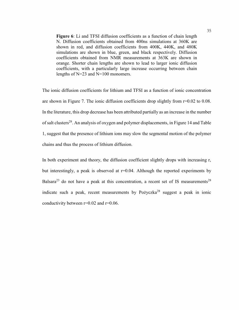
Figure 6: Li and TFSI diffusion coefficients as a function of chain length

N. Diffusion coefficients obtained from 400ns simulations at 360K are

shown in red, and diffusion coefficients from 400K, 440K, and 480K

simulations are shown in blue, green, and black respectively. Diffusion

coefficients obtained from NMR measurements at 363K are shown in

orange. Shorter chain lengths are shown to lead to larger ionic diffusion

coefficients, with a particularly large increase occurring between chain

lengths of N=23 and N=100 monomers.

The ionic diffusion coefficients for lithium and TFSI as a function of ionic concentration

are shown in Figure 7. The ionic diffusion coefficients drop slightly from r=0.02 to 0.08.

In the literature, this drop decrease has been attributed partially as an increase in the number

of salt clusters28. An analysis of oxygen and polymer displacements, in Figure 14 and Table

1, suggest that the presence of lithium ions may slow the segmental motion of the polymer

chains and thus the process of lithium diffusion.

In both experiment and theory, the diffusion coefficient slightly drops with increasing r,

but interestingly, a peak is observed at r=0.04. Although the reported experiments by

Balsara23 do not have a peak at this concentration, a recent set of IS measurements28

indicate such a peak, recent measurements by Pożyczka28 suggest a peak in ionic

conductivity between r=0.02 and r=0.06.

36

Figure 7: Li and TFSI diffusion coefficients over a range of concentrations,

r=0.02, 0.04, 0.06, and 0.08 (Li:EO). Diffusion coefficients obtained from

molecular dynamics simulations at 360K, 400K, 440K, and 480K are shown

in red, blue, green, and black, respectively. Diffusion coefficients obtained

from NMR experiments at 363K are shown in orange and IS experiments at

373K are shown in purple. The overall diffusion coefficient is shown to

decrease slightly with ionic concentration. The computed diffusion

coefficients lie within the experimental range.

The activation energies for lithium and TFSI diffusion are shown in figure 8 as a function of

chain length and ionic concentration. These values are in the range reported by Gorecki1, and

suggest that the computed diffusion coefficients are transferable across a range of

temperatures.

37

Figure 8: Li and TFSI activation energies over a range of chain lengths,

N=23, 45, 100, 450, and concentrations r=0.02, 0.04, 0.06 and 0.08 Li:EO.

The computed activation energy depends weakly on chain length and

concentration within this regime, in agreement with experimental

measurements1.

To understand the atomistic nature of diffusion, the coordination model is then used to

analyze the atoms with the largest and smallest mean-squared-displacements (MSD) over

the simulation time. These atoms are denoted as the most and least diffusive lithium. The

chain coordination of the most diffusive lithium atom in the r=0.02 Li:EO, N=100

simulation at 360K is plotted as a function of time in Figure 9. The structure on the right

shows the real space position of this single lithium atom evolving over time, over 0.25ns

intervals. The lithium resides on the 8th chain for around 30ns before hopping to the 9th

chain, then the 5th. Overall, the most diffusive lithium moves 59.3Å in 400ns and

coordinates to a total of seven chains.

Figure 9: Examines the coordination and displacement behavior of the

single most diffusive lithium atom in the 360K/20LiTFSI/N=100

simulation as a function of time. The plot on the left shows the most

coordinated chain as a function of time throughout the 400ns simulation.

Most Diffusive Lithium, 360K/20LiTFSI

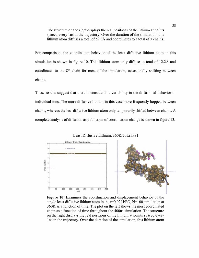
38

The structure on the right displays the real positions of the lithium at points

spaced every 1ns in the trajectory. Over the duration of the simulation, this

lithium atom diffuses a total of 59.3Å and coordinates to a total of 7 chains.

For comparison, the coordination behavior of the least diffusive lithium atom in this

simulation is shown in figure 10. This lithium atom only diffuses a total of 12.2Å and

coordinates to the 8th chain for most of the simulation, occasionally shifting between

chains.

These results suggest that there is considerable variability in the diffusional behavior of

individual ions. The more diffusive lithium in this case more frequently hopped between

chains, whereas the less diffusive lithium atom only temporarily shifted between chains. A

complete analysis of diffusion as a function of coordination change is shown in figure 13.

Figure 10: Examines the coordination and displacement behavior of the

single least diffusive lithium atom in the r=0.02Li:EO, N=100 simulation at

360K as a function of time. The plot on the left shows the most coordinated

chain as a function of time throughout the 400ns simulation. The structure

on the right displays the real positions of the lithium at points spaced every

1ns in the trajectory. Over the duration of the simulation, this lithium atom

Least Diffusive Lithium, 360K/20LiTFSI

39

diffuses a total of 12.2Å and remains primarily coordinated to chain #8 for

the majority of the simulation.

This analysis was repeated for the most and least diffusive lithium atoms for the r=0.02

Li:EO, N=100 simulation at 480K and the results are shown in figures 11 and 12. At this

temperature, numerous interchain hops are observed over the 115ns trajectory and the total

displacements of the lithium are 115.4Å and 45.5Å, respectively. These results suggest a

change in the mechanism for diffusion at higher temperatures, as lithium are more able to

overcome the barriers for interchain diffusion. This mechanism is analyzed in terms of the

hopping model, shown in figure 3, in the discussion section.

Figure 11: Examines the coordination and displacement behavior of the

single most diffusive lithium atom in the 480K/20LiTFSI/N=100

simulation as a function of time. The plot on the left shows the most

coordinated chain as a function of time throughout the 115ns simulation.

The structure on the right displays the real positions of the lithium at points

spaced every 1ns in the trajectory. Over the duration of the simulation, this

lithium atom diffuses a total of diffuses a total of 115.4Å with frequent hops

between all 10 PEO chains.

Most Diffusive Lithium, 480K/20LiTFSI

40

Figure 12: Examines the coordination and displacement behavior of the

single least diffusive lithium atom in the r=0.02, N=100 simulation at 480K

as a function of time. The plot on the left shows the most coordinated chain

as a function of time throughout the 115ns simulation. The structure on the

right displays the real positions of the lithium at points spaced every 0.25ns

in the trajectory. Over the duration of the simulation, this lithium atom

diffuses a total of diffuses a total of 45.5Å with frequent hopping between

all 10 PEO chains.

Discussion

The changes in chain coordination of the most and least diffusive lithium atoms suggest a

connection between chain coordination and total lithium displacement. In order to examine

this, changes in lithium coordination are tracked every ∆t=0.25ns in the trajectory. The

hopping model, shown in figure 3, describes lithium motion as intrachain diffusion,

interchain “hops” between chains, and interchain “shifts” when lithum remains coordinated

to multiple chains.

An analysis of the lithium coordination frequency is shown as a function of temperature in

figure 13. A small number of lithium atoms undergo no change in coordination, ∆n=0.

Least Diffusive Lithium, 480K/20LiTFSI

41

Small intrachain hops, ∆n≤1, correspond to slight changes in the lithium-oxygen

coordination shell and are the frequent transition at lower temperatures T=360K, 400K,

440K. Increases in temperature are correlated with an increased frequency of large

intrachain hops, ∆n>2 and interchain hops, which suggests that an activation barrier is

associated with these processes. Interestingly, the frequency of shifts is seen to be

independent of temperature, suggesting that this coordination pattern is geometric in nature

rather than energy-mediated. The lithium displacements corresponding to these processes

are shown in figure 14.

Figure 13: Frequency of lithium coordination changes as a function of

temperature. Small intrachain hops, ∆n≤1, are most frequent at lower

temperatures T=360K, 400K, 440K. Increases in temperature are correlated

with an increased frequency of large intrachain hops, ∆n>2 and interchain

hops. Interestingly, the frequency of shifts is seen to be independent of

temperature, suggesting that this coordination pattern is geometric in nature

42

rather than energy-mediated. The lithium displacements corresponding to

these processes are shown in figure 14.

The displacements associated with each of these diffusion processes are shown in figure

14. For no change in coordination, the lithium displacements, ∆n=0 caused by the

segmental motion of the polymer chains. This segmental motion is shown to be the

dominant contributor to ionic diffusion over short timescales. Intrachain changes in

coordination along a chain (∆n>0) contribute to the overall lithium diffusion, but intrachain

hops alone are not enough to reach the Fickian diffusion limit. Interchain hops, on the other

hand are correlated with the largest increases in lithium motion and contribute significantly

to the diffusion process. Taken together, these results suggest that the atomistic nature of

lithium diffusion is consistent with the Rouse93 model formulation – the segmental motion

of polymer chains drives is associated significant vehicular diffusion. Frequent lithium

43

intrachain hops and infrequent interchain hops contribute to the overall diffusion

process.

Figure 14: Average lithium displacements associated with coordination

change. The ∆n=0 displacement is associated with the vehicular motion of

the polymer backbone. The increase in average displacements for ∆n>0 is

associated with intrachain diffusion along a chain. Interchain hopping is

associated with significantly increased diffusion.

In order to examine the nature of segmental motion of the polymer chain, the displacement

of individual oxygen atoms are analyzed. As polymer displacements can differ as a function

of chain position, the two extreme cases are considered – oxygen atoms located at the center

of the chain (n=50, 51) and oxygen atoms located at the edge of the chain (n=1, 100). The

results of this analysis are shown in table 1. Across all temperatures, it is shown that the

oxygen atoms near the edge of the polymer chain diffuse ~30% more than the oxygen atoms

44

at the center of the chain. This suggests increased polymer flexibility and motion for

shorter chains, consistent with the results of the diffusion simulations.

Table 1: Shows real space oxygen of polymer backbone oxygen over

timescales of ∆t=0.25ns. Average displacements are taken for the two

oxygen sites closest to center (n=50, 51) and edge (n=1, 100) of a length

N=100 polymer chain. These results suggest an increase in segmental

motion at the edges of the polymer chain. These results also suggest that the

presence of lithium ions may slow the segmental motion of the polymer as

the displacements of the polymer chain is significantly less than the ∆n=0

motion of lithium at a fixed site along the chain.

Interestingly, it is observed that the oxygen along a polymer chain diffuse significantly more,

on average, than the lithium atoms at a fixed position along a chain (∆n=0), as seen in figure

14. This suggests that the presence of lithium ions may constrain the motion of the polymer

and reduce the segmental motion of the polymer associated with the thermal reptation of the

polymer. This effect could explain the reduction in ionic diffusion coefficients observed at

higher ionic concentrations.

The reduction in chain motion in the presence of lithium ions also suggests that lithium

coordinated to multiple chains (i.e. shifting), may slow the overall rate of segmental diffusion

in the polymer. This is consistent with the increased number of shift transitions associated

Oxygen Displacements (∆t=0.25ns)

Displacement Center Edge

360K 3.0Å 3.8Å

400K 4.8Å 6.3Å

440K 6.5Å 8.8Å

480K 7.6Å 10.4Å

45

with the least diffusive lithium ions in figures 10 and 12. This suggests that the nature of

lithium coordination between chains may play an important role in ionic diffusion.

Conclusions

Taken as a whole, these results show that both the motion of polymer backbone and

interchain hopping make the largest instantaneous contributions to polymer diffusion.

Intrachain motion makes a smaller instantaneous contribution to diffusion, but is the most

probable mode near the battery operating temperature around 360K. An analysis of oxygen

displacements suggests that the presence of lithium may slow polymer reptation,

particularly when the lithium is coordinated to multiple chains. The results also suggest

that lithium atoms can reside between chains and that interchain hops must involve both

coordination to a new chain and detachment from its previous chain in order to facilitate

greater ionic diffusion. Additionally, reasonably accurate relative ionic diffusion

coefficients, consistent with experimental data, were obtained across a range of ion

concentrations, temperatures, and molecular weights. The obtained results validate that this

methodology shows promise for predicting the structure and ionic conductivity of new and

novel polymer materials.

46

C h a p t e r I I I

POLARIZABLE CHARGE EQUILIBRATION METHOD (PQEQ)

With contributions from Saber Naserifar, William A. Goddard III, and Vaclav Cvcivek

Acknowledgement: The main part of this chapter is published in the Journal of Chemical Physics, 2017, 146(12), pp124117.

Abstract

Electrostatic interactions play a critical role in determining the properties, structures, and

dynamics of chemical, biochemical, and material systems. These interactions are described

well at the level of quantum mechanics (QM) but not so well for the various models used in

force field simulations of these systems. We propose and validate a new general

methodology, denoted PQEq, to predict rapidly and dynamically the atomic charges and

polarization underlying the electrostatic interactions. Here the polarization is described using

an atomic sized Gaussian shaped electron density that can polarize away from the core in

response to internal and external electric fields, while at the same time adjusting the charge

on each core (described as a Gaussian function) so as to achieve a constant chemical potential

across all atoms of the system. The parameters for PQEq are derived from experimental

atomic properties of all elements up to Nobelium (atomic no. =102). We validate PQEq by

comparing to QM interaction energy as probe dipoles are brought along various directions

up to 30 molecules containing H, C, N, O, F, Si, P, S, and Cl atoms. We find that PQEq

predicts interaction energies in excellent agreement with QM, much better than other

common charge models such as obtained from QM using Mulliken or ESP charges and those

from standard force fields (OPLS and AMBER). Since PQEq increases the accuracy of

47

electrostatic interactions and the response to external electric fields we expect that PQEq will

be useful for a large range of applications including ligand docking to proteins, catalytic

reactions, electrocatalysis, ferroelectrics, and the growth of ceramics and films, where it

could be incorporated into standard force fields such as OPLS, AMBER, CHARMM,

Dreiding, ReaxFF, and UFF.

1. Introduction

For practical simulations of dynamical processes, such as ligands binding to

proteins, nucleic acids, and polymers responding to externals fields and stresses,

catalysts reacting with substrates, and external fields driving electrochemical

reactions, it is necessary to go far beyond the time and length scales of QM through

the use of a force field (FF) to describe the structures and forces as they evolve. A

critical issue in all such multiscale models is how to accurately describe

electrostatic interactions. One common approach is to break the system into

fragments, perform QM calculations on each one, and then obtain partial charges

from Electrostatic Potential fitting (ESP)100, Mulliken Population Analysis

(MPA)101 or other QM charge assignment models102. Additional discussion on

these models can be found in the Supplementary Materials. One disadvantage with

these approaches is that the charges are fixed and not allowed to adjust to changes

in the electrostatic environment that occur during dynamics. It can also be

burdensome to perform the QM calculations to obtain charges, for example, for

the millions of ligands used in Virtual Screening (VS) applications.

The charge equilibration (QEq)103 method introduced by Rappé and Goddard in

1991 provides an alternative fast way to predict charges for systems too large for

48

QM. Indeed, carrying out the QEq calculation along an MD trajectory takes into

account some changes in polarization during dynamics. Advantages of QEq are

that the 3 parameters per atom are derived from atomic ionization energies

(valence averaged) and from covalent radii so that they are available for the whole

periodic table (through Lr, atomic no. =103). Also, because the charge on each

atom is distributed over a Slater orbital having the size of the atom, QEq can be

used to predict charges between bonded atoms to describe the changes during

reactions. This made QEq useful for defining a general FF (UFF) 104 for inorganic-

organic systems and for reactive FFs (ReaxFF)105, 106. However, it has not been

demonstrated whether QEq is as accurate as ESP or MPA in reproducing QM

energies nor that the predicted changes in polarization during dynamics agree with

QM.

Describing the changes in polarization within a molecule or solid during dynamics

or in response to an external electric field is crucial in many applications 107-109.

Consequently, many strategies have been proposed for including polarization into

FFs particularly for liquid water and its interactions with ions 110-113, for modeling

of proteins114-118, DNA119, enzymatic reactions120, protein–ligand docking121, 122,

peptides123, and in small-molecule systems124-132. Polarization is also important in

ion channels and aqueous solution111, 133-135, superionic systems136, piezoelectric

and ferroelectrics materials137-139, lithium batteries140, crystal defects and surface

energies141-143, lattice vibrational frequencies calculations143, 144, dynamic

dielectric response or Raman light scattering144, 145, hydration energy

calculations146, carbon nanotubes147, and predicting organic crystal structure 148-

49

151. This need has led to a number of approaches that have been discussed

thoroughly in several reviews107, 108, 110, 152-154. Our perspectives about these

methods is summarized in the Appendix D.

In this paper, we propose a new polarizable charge equilibration scheme that build s

upon the success of QEq and includes polarization in a generic way that can be

easily extended for the entire periodic table. This polarizable charge equilibration

model (PQEq) allows charges and polarization to readjust dynamically to attain a

constant chemical potential during the simulation. Here the polarization is

described by an atomic sized Gaussian shaped electron density cloud that can

polarize away from the atomic core in response to internal and external electric

fields. The charges on the cores are also described by Gauss ian functions and

charge can flow from one atom to another based on the QEq charge equilibration

scheme. The total electrostatic energy is expressed as a sum of internal atomic

energy plus pairwise shielded Coulombic interactions. PQEq uses the same

covalent bond radii and atomic ionization energies previously used in QEq. An

additional atomic polarization parameter is based on the literature value for atomic

polarizability. Thus, the parameters for PQEq are well defined for all elements up

to Nobelium (atomic no. =102).

For validation, we perform a series of high quality QM calculations for 30

structures using cyclohexane and benzene scaffolds containing H, C, N, O, F, Si,

P, S, and Cl atoms. The interaction energy was computed by bringing a pair of ±1

point charges (probe dipole) towards each structure along several axes. We show

that PQEq produces interaction energies in excellent agreement with QM. In

50

addition, we optimize a parameter set (PQEq1) that increases the accuracy in the

interaction energies for these particular compounds. Here, and for the rest of the

paper, the total interaction energy between the dipole and target structure is

referred to as the interaction energy. For fixed charge models, this interaction is

just the electrostatic energy between the dipole and fixed charges (i.e. no

polarization). For PQEq, with charge updates and shell polarization turned on, this

interaction energy now also reflects the change in energy from polarization.

We then compare the PQEq interaction energies with other common charge models

such as Mulliken or ESP charges obtained from QM and those from standard force

fields (OPLS155-158 and AMBER159-161). We find that the fixed charge methods do

not describe the induced polarization in the system.

Based on these results, we believe that PQEq can be used to improve the

description of electrostatic interactions for systems in which polarization is

important. It can be incorporated into existing force fields such as OPLS, AMBER,

CHARMM162-164, Dreiding, ReaxFF, and UFF, but it may be necessary to modify

some parameters to account for the change in the charge model. This could be

useful for a large range of applications including ligand docking to proteins,

catalytic reactions, electrocatalysis, ferroelectrics, and growth of ceramics and

films.

2. Methods

2.1 Polarizable Charge Equilibration (PQEq) model

The PQEq model combines the QEq103 charge equilibration model with the shell

(Drude oscillator) model114, 129, 138, 165, 166. The key difference from previous shell

51

models is that PQEq does not use point charges. Rather the shell electron is

described as a Gaussian function having the same size as the core charge. This

leads to shielding as the shell electron interacts with its core and with other atoms

so that the singularities in point charge descriptions are avoided. The polarization

of the shell away from its core in response to the electrostatic field of all other

charges and any external field accounts for polarization dynamically. Here we take

the mass of the shell to be zero so that it responds adiabatically as the atoms move

about in the MD.

For a system of N atoms, each atom, i, is partitioned into two charged sites (core

and shell). The core (ρic) consists of two parts; ρi with a variable total charge (qi)

and ρiZ with a fixed total charge (Zi). The shell (ρis) has a fixed total charge of -Zi.

The shell and core of an atom are connected by an isotropic harmonic spring with

force constant Ks (see Figure 1),

,

2

1 2RKE s

(1)

where R is the distance between the core and shell. Equation 1 leads to an atomic

or shell polarizability of

,

2

s

unitK

ZC (2)

,

2

ZCK units

(3)

where Z is the shell charge and Cunit = 332.0637 is a unit conversion factor that

expresses energy in kcal/mol, distance in angstroms (Å), and η as Å3. This

conversion constant is Cunit =14.3994 for energies expressed in eV. The η values

52

derived from the atomic polarizability can be computed using high quality ab-

initio calculations or measured for single atom polarization in response to an

external electric field. We use the values tabulated by Miller167.

Defining the total charge (core plus shell) on atom i as qi, the individual charges

on the core and shell are

.

,

iis

iiic

Zq

Zqq

(10)

The net atomic charge at the core ( iicis qqq ) is variable and adjusts to keep the

chemical potential constant. There is positive fixed charge (Zi) at the core at

position icr

(i.e. ir

) and a negative fixed charge (-Zi) is at the shell position isr

. The

displacement of shell i with respect to its core, icisr ,

, is defined as icis rr

. The charge

density of both the core and the shell is described by a 1s Gaussian charge

distribution,

),()()( rrr iZiic

(11)

),()( rrZiis

(12)

,exp)(2

23

iciii

i rrqr

(13)

,exp)(2

23

iciZiiZ

iZ rrZr

(14)

,exp)(2

23

isiZi

iZ

ZirrZr

(15)

where ik , the width of the distribution, is given by

53

.2 2

ik

ikR

(10)

Here, Rik is the covalent atomic radius in Å units and λ is a parameter that converts

the overlap of two Gaussian charges to the effective shielding. We determined the

value of λ by comparing PQEq and QM electrostatic interaction energies (see

below). The PQEq model uses equal atomic and shell radii (i.e. Ri=Ric=Ris) for

each atom i so that the above equations simplify to

,exp)()()(2

23

iciiii

iZiic rrZqrrr

(16)

.exp)(2

23

isiii

is rrZr

(17)

This charge distribution has the shape of a spherical 1s Gaussian shape with a

width determined by the atomic radius of the atom. The core and shell of each

atom has a Columbic interaction with the cores and shells of every other atom in

the system. We allow the atomic charges (qi) to respond to the electrostatic

environment based on the QEq scheme103, 139. The position of the shell is then

calculated by balancing the sum of all electrostatic forces on the shell with the

spring force (see below). A shell charge of Zi=1 is used for all atoms.

54

Figure 1: Partition of a two-atom system into core and shell for the

PQEq model. Both cores and shells are described by spherical 1s

Gaussian charge distributions. The core (ρic) consists of two parts; ρi

with a variable total charge (qi) and ρiZ with a fixed total charge (Zi).

The shell (ρis) has a fixed total charge of -Zi. The shell and core of

an atom interact with each other through a harmonic spring force.

Cores and shells of different atoms interact with each other through

Coulombic interactions as well. The atomic charge on each core (qi)

is allowed flow within the system until the atomic chemical

potentials are equalized.

2.2 Electrostatic Energy

The electrostatic energy between two Gaussian charges is given by jlikjlik qqrC

, ,

where

,

1.

ik jl

ik jl

ik jl

C r erf rr

(18)

Here i and j are the atomic indices, and k and l represent the core (c) and shell (s),

respectively. In the case of jlik rr

, jlikC , is equal to

55

.2

lim ,0

0

,

jlik

jlik

jlikr

jlik =rCC

(19)

A well-known problem in other shell and induced dipole120, 168 models is that they

suffer from a polarization catastrophe when the shells or dipoles are placed too

close together. The Gaussian shielding present in PQEq addresses this issue as the

Coulombic interaction energy remains finite, even in the limit of zero interatomic

distance.

We describe the PQEq electrostatic energy, iisic qrrE ,,

, as a sum of an intra-

atomic electrostatic energy iisici qrrE ,,

and interatomic pairwise Coulomb

interactions,

ji

jlikjlikjlik

N

i

iicisiiisic qqrCqrEqrrE .,,, ,,,

(20)

The internal energy (Ei) is a function of the electronic polarization and total charge

on the atom.

.,, ,, iiiicisiiiiicisi q0,EqrEq0,EqrE

(21)

The first term on the right hand side of Equation 21, ii qE ,0 is the energy required

to create a charge, qi, assuming zero polarization and neutral atomic state as the

reference point. We use a Taylor expansion to express this energy term as

...2

1

0

2

22

0

0

i

i

i

iiiiq

Eq

q

EqEq0,E

(22)

and truncate it after second-order terms. The original QEq method103 included a

radius dependent scaling parameter for hydrogen atom in order to better fit the

56

dipole moment for both alkali hydrides (e.g., LiH) and halogen hydrides (e.g., HF).

This leads to a nonharmonic dependence of energy, which in our experience can

lead to unstable systems, so PQEq eschews this complication.

We use three conditions to determine the rest of the parameters as follows:

,

2

11

0

2

2

0

0

ii

iiq

E

q

EE0,E

(23)

,0 0

ii E0,E (24)

.2

1

0

2

2

0

0

ii

iiq

E

q

EE0,-1E

(25)

Here, 10,iE is the ionization potential (IP), which is the energy required to

remove one electron from the atom, and 10,iE is the electron affinity (EA),

which is the energy gained when an atom receives one additional electron. Both

IP and EA are well known experimentally for nearly all elements. We use the same

values as determined by Rappé and Goddard103 in which the experimental IP and

EA are averaged over the ground state atomic configuration in order to reflect the

averaging introduced by bonding to other atoms. Thus, for nitrogen atom the IP

and EA are derived using the averages over the 4S, 2D, and 2P states associated

with the (2s)2(2p)3 configuration and the 3P, 1D, and 1S states associated with the

(2s)2(2p)2 and (2s)2(2p)4 configurations of the ions. Solving Equations 23-25 for

the unknowns yields

,

21

0

0

i

iq

EEAIP

(26)

57

,

0

2

20

i

iiq

EEAIPJ

(27)

where 0

i is the Mulliken electronegativity169 of atom i and 0

iiJ is the idempotential

(hardness) or electron capacity of atom i, which resists electron flow to or from an

atom. We replace the second term on the right hand side of Equation 21 with the

Coulombic interaction between core and shell of atom i plus a spring interaction

between the core and shell of atom i. Therefore, Equation 20 can be written as,

.2

1

2

1, 2

,

32000

, isicsiiiiiiiiicisi rKqOqJqEqrE

(23)

Ignoring the 3

iqO term in Equation 23, the electrostatic energy of the system is

given by

,2

1

2

1},,{ ,,

2

,

2000

jlik

jlikjlikjlikisics

N

i

iiiiiiiisic qqrCrKqJqEqrrE

(24)

where the second sum is the pairwise shielded Coulomb interaction energy

between all cores and shells, which can be expanded to give the total electrostatic

energy as

.)()()()(

2

1

2

1},,{

,,,,

2

,

2000

jijsisijcjcis

ji

jicjsicjcicjcic

isics

N

i

iiiiiiiisic

ZZrCZqrCZqrCqqrC

rKqJqEqrrE

(28)

2.3 The Charge Equilibration Condition

A serious problem in most classical MD/MM applications is that fixed charges are

assigned to each atom. Such fixed charges (even the most reliable ones from ab-

initio calculations) do not respond to the changes in the electrostatic environment,

58

which decreases the accuracy. This problem becomes paramount for reactive force

fields (e.g. ReaxFF106) where the bond connectivities of atoms change during

reactive MD simulations, requiring updates of the atomic charges (ideally at each

time step). As in QEq, the PQEq model allows the charge distribution on the

various atoms to change as the electrostatic environment changes during the

dynamics. The optimum charge distribution is computed from the conditions that

the chemical potentials ( iqE / ) are equal for all of the atoms (which provides N-

1 conditions where N is the number of atoms) and that the total charge is conserved

,Qqqqi

i

i

isic

(29)

where Q is the total charge of the system. We use Lagrange multipliers to

guarantee this constraint as the charges are optimized. The energy expressions with

the Lagrange multiplier, µ, is

{ , , , } { , , } .ic is i ic is i i

i

E r r q E r r q q (30)

Setting the derivative of Equation 30 equal to zero yields

,0

ij jij

i

AqHq

E

(31)

),(1 ,

0

jcicijijiiij rCJH

(32)

ji

jjsicjcicii ZrCrCA ,)()( ,,

0

(33)

where Hij is an N by N matrix and δij is the Kronecker delta function. The diagonal

elements of Hij matrix (δij =1) denote the idempotential of the atoms while the off-

diagonal elements represent the Coulombic interactions between the variable

charge part of the cores (i.e. qi). Ai in Equation 33 is a vector of length N. The first

59

term of Ai is the electronegativity of the atom. The second term is the Coulombic

interaction coefficient between the core and shell of the atom i. The third term is

the sum of Coulombic interaction coefficient between variable charge part of core

i (i.e., qi) and the fixed charge component of all other cores and shells (i.e., Zj and

–Zj). Note that in Equation 33, Ai is a fixed quantity for each atom during the

charge minimization, which reduces to 0

iiA if polarization is not included, as

in the QEq model103, 170. In Equations 31-33, the Lagrange multiplier μ is the

chemical potential that constrains the sum of the atomic charges to be equal to the

total charge of Q. Solving Equations 31-33 leads to

).1(1

jj

j

iji AHq

(34)

Applying Equation 29 we get

,11

i j

ij

i

j

j

ij

i

i QHAHq

(35)

which is solved to obtain μ

1

1,

ˆ1

ij j ii j i

ij j i

i j i

Q H A q

H q

(36)

where iq~ and iq̂ are fictitious charges. In practice, we solve Equation 36 by

partitioning it into two sub equations. Setting the derivative of Equation 36 to zero

results in

,~ij

j

ij AqH

(37)

.1ˆ j

j

ijqH

(38)

60

Finally, the instantaneous total charges on each atom (qi=qic+qis) can be written

as

.ˆ~iii qqq

(39)

The above formulation for PQEq omits the presence of external electric fields,

which is included in the Supplementary Materials. A frequency-dependent

response can be obtained from time-dependent fields.

2.4 Preconditioned Conjugate Gradient (PCG) Solution of the Charge

Equilibration Equations

Exactly solving for the charges that satisfy the QEq condition involves inverting

an N by N matrix, which scales as O(N3). Since this is required every time step103,

this process is computationally too expensive to be practical for large systems. A

practical solution to this problem is the PCG method implemented in the

PuReMD171, 172 and LAMMPS173 software packages.

We use PCG to solve Equations 37 and 38. The efficiency and convergence of this

iterative conjugate-gradient (CG) method depends on the spectrum of the

coefficient matrix. The PCG method uses a second matrix (preconditioner) to

transform the coefficient matrix to obtain improved spectral properties. This

preconditioner involves an incomplete factorization of the coefficient matrix. In

particular, incomplete LU factorization (ILU) (where L and U are lower and upper

triangular) can be used for solving this sparse linear systems 174. For QEq, Aktulga

et al. studied the performance, stability, and accuracy of the ILU-based

preconditioners for various model systems172. They showed that ILU-based

61

preconditioners dramatically reduces the number of iterations while allowing the

same L and U factors to be used effectively as preconditioners over several steps,

due to the slow changes in the simulation environment. We extended this ILU -

based preconditioner method to PQEq and coupled it with shell relaxation (see

next section) to calculate the PQEq charges while updating the shell position.

2.5 Shell Relaxation

In our formulation of the PQEq dynamics, we choose to displace the core of each

atom together with its shells as a rigid body during every timestep of the dynamics.

After moving core plus shell, the first step of the next iteration is to calculate the

electrostatic field on every particle and to solve the PQEq equations (using the

PCG method) for the new charges. Next, we fix the core positions and update the

positions of all shells simultaneously using a one-step relaxation as follows. If

necessary, this process of updating atomic charges and shell relaxation with fixed

cores can be repeated for several iterations to attain self-consistency for

troublesome geometries. However, we find that one cycle is normally sufficient to

reach equilibrium for each timestep after the first.

The shell position for each atom is obtained by balancing the effect of the

electrostatic field due to all external atoms with intra-atomic interactions

involving only the core and its shell. These forces are calculated by taking the

derivative of the electrostatic energy (Equation 28) with respect to the shell

position,

62

,2

1 2

,

isics

is

intra rKr

F

(40)

.)()()()( ,,,, jijsisijcjcis

j

jicjsicjcicjcic

is

external ZZrCZqrCZqrCqqrCr

F

(41)

We solve Equations 40 and 41 to find the optimal position of shells (ris) using a

single iteration of the Newton-Raphson method. Since the shell is typically very

close to its core (usually < 0.1 Å), we neglect the effect of the external core and

shell charges on this second derivative to avoid inverting the Hessian. We assume

here that the shell is massless, so that it relaxes instantaneously to its zero-force

position, with no inertial delay. Therefore, we estimate the new position of the

shell by assuming that Fintra and Fexternal are collinear. Thus, the new position of

the shell is computed by,

,)(

)(

,

,

22,

,

,

,,

oldis

oldis

ris

rexternalintra

oldis

oldis

oldis

oldisnewis

rE

FFr

rE

rErr

(42)

.2

1 2

,2

2

2

2

isics

isis

rKrr

E

(43)

Although, this problem is not strictly one-dimensional, we use the above second

derivative allowing the shell to rotate into the direction in which the external field

acts.

3. QM Interaction Energy for Validation

In order to validate the accuracy of PQEq and to perform optimization of the model

(if needed), we must decide the criteria to use for comparison and optimization.

The normal practice in most FFs is to use QM charges. We discuss in

63

Supplementary Materials that QM charges are not reliable for this purpose.

Instead, we use the QM interaction energy. We probe each of the 30 molecules in

our validation set with a pair of ±1 point charges separated by 1 Å to describe the

interaction with dipole and higher order multipoles. For convenience, we refer to

this pair of point charges as an electric dipole. The interaction energy from QM is

shown as a function of distance and used as the reference energy.

We selected scan axes along a variety of symmetry directions to provide insight

about how the polarization depends on the elements. Care was taken to avoid close

contacts with the nearby atoms. Figure 2 shows an example for cyclohexane

molecule of electric dipole scans along several different directions. These scans

are performed towards a backbone atom (d1 and d2), along a bond (d3 and d4),

perpendicular to a bond (d5), and toward the center of mass of the structure (d6).

For all calculations, we use the standard B3LYP hybrid flavor of DFT, including

both the generalized gradient approximation and a component of the exact

Hartree–Fock (HF) exchange175-179. These calculations were performed with the 6-

311G(d,p) (or 6-311G**++) basis set180.

64

Figure 2: Interaction energies from bringing an electric dipole toward

the cyclohexane molecule along various directions including: toward

C and H atoms (d1 and d2), along a C-H bond (d3 and d4),

perpendicular to a C-C bond (d5), and toward the center of mass (d6).

The positive (red) and negative (blue) heads of the dipole form an

angle of 180° (dotted line) with the reference point. The

corresponding directions are labeled on the molecular configuration

shown in the inset of the figure. Note that for most directions, the

QM energies increase below 1.5 Å due to non-electrostatic effects.

4. PQEq Database

We used a set of 30 molecular structures in our validation of the PQEq model. We

designed this data set to cover H, C, N, O, F, Si, P, S, and Cl elements in a balanced

manner. These structures are depicted in Figure S3 of the Supplementary

Materials. We use cyclohexane and benzene rings as the framework for these

molecular structures, replacing C and H with the above atoms. This framework

provides a reasonable number of atoms and bond types for studying charge transfer

65

and polarization effects. The molecular structures are at their equilibrium

geometries optimized using QM with same DFT method and basis set described

above. Then, the electric dipole is scanned along various directions with respect

to these molecular structures. The scan directions were selected after extensive

preliminary calculations to probe properly the amount of polarization and

electrostatic potential change during the scan. We excluded cases that resulted in

less than 2 kcal/mol change in the energy throughout the scan. We also avoided

scanning directions that could lead to very close interaction of the dipole with

nearby atoms. In addition, to avoid non-electrostatic interactions arising from

Pauli principle repulsion at close distances we scan only up to the inflection point

(attractive forces) of the electrostatic potential curve. We find this distance to be

near 2.5 Å for most of the cases so that the electric dipole is scanned from 10.0 Å

up to 2.5 Å with respect to the reference point for all cases.

The above considerations resulted in a total of 68 scans for the above molecular

structures. The change of QM electric dipole energy with the distance for each

case is shown in Figure S4 of Appendix D.

5. Results

5.1 Parametrization of PQEq Model

In this paper, we present two sets of PQEq parameters. The first set (denoted as

PQEq) uses the same χ, J, and Rcs parameters as in the QEq method103 which were

obtained from standard bond radii and experimental ionization energies. These are

available for all elements of the periodic table up to Lawrencium (Lr) (atomic no.

66

=103). Using Equation 3, we derived the Ks values based on experimental or high

quality ab-initio calculations of atomic polarizabilities in the presence of an

external electric field. These values are available up to Nobelium (No) (atomic no.

=102)167. The exception is for H atom where we use IP=11.02 eV and EA=1.96 eV

to define χ and J as did Rappé and Goddard103 and we take the Ks value for H from

the Karasawa and Goddard calculation for the polarizability of Polyvinylidene-

fluoride crystal that they fitted to a shell-model138. Our results in the next section

show that this default PQEq parameter set, with no addit ional optimization predicts

interaction energies from QM very well.

For the second series of parameters (PQEq1), we performed a constrained

optimization of the atomic χ and J parameters with respect to the QM derived

energy for all 68 cases. We used CG optimization to minimize the difference

between the energies computed by PQEq1 and QM. The total error is defined as

the weighted mean square error (MSE),

2

1 ,i QM PQEq

i

Error E E (44)

where ωi is the weight and EPQEq and EQM are the energies computed by PQEq1

and QM, respectively. Constraints were applied to ensure that the parameters obey

the general trends of the periodic table. That is, we require that within a row of

the periodic table the atoms should become more electronegative as we move to

the right. Similarly, we require atoms become more electronegative as we move

down a column in the periodic table. This was enforced at each step of th e

optimization. These constraints defend against overfitting and ensure better

transferability of the final parameter set. We find the total error in Equation 44 to

67

decrease from 1219.29 to 471.55 during the PQEq1 optimization. Thus for this

class of systems the PQEq1 parameters should provide a more accurate description

of the electrostatics. The changes in parameter values are generally small. The

maximum change in the PQEq1 parameters is for Fluorine (F) atom, which led to

a 19.96 percent change in the χ parameter. The comparison between the parameters

before and after optimization is shown in Table S3 in the Supplementary Materials.

The PQEq and PQEq1 parameters are tabulated in Table S1 and Table S2 in the

Supplementary Materials, respectively. We also provide the electronic versions of

these files.

5.2 Electric Dipole Energy

Figure 3 shows the comparison (one for each atom type) between the interaction

energies computed by QM, PQEq, and PQEq1 for the scan of the electric dipole at

different distances. Here, the interaction energy includes the polarization effect

during the scan. The dipole scan directions are shown with the dotted lines on the

molecular structure schematics for each case. Comparisons for additional cases are

shown in Figure S4 of Appendix D.

Based on these results, we choose the effective shielding parameter in the Equation

10 to be λ=0.4628. This value is close to the corresponding number in QEq model

(0.4913) using Slater-type orbitals103. The results show good agreement of PQEq

with QM. This suggests that the PQEq general parameter set can accurately

describe the electrostatic potential for a variety of molecular structures and

environments. Thus, we expect good transferability of the PQEq model to new

68

materials. This often has been a challenge for previous FFs and charge calculation

models. As expected, the results from PQEq1 parameter set show better agreement

with QM and may be useful for other systems contain similar structures as in our

database. In particular, PQEq1 provides a dramatic improvement for molecules

containing Fluorine element, as seen in Figure 3e

Figure 3: Interaction energies of an electric dipole near database molecular structures computed by QM (blue), PQEq (red), and PQEq1 (green). One case is presented for each atom type; (a) H, (b) C, (c) N, (d) O, (e) N and O, (e) F, (f) Si, (g) P, (h) S, and (i) Cl. The inset of each subfigure shows the molecular structure configuration with the scan direction (dotted line) of the electric dipole. The ±1 electric dipole is shown with small solid spheres. The positive (red) and negative (blue) heads of the dipole form an angle of 180° (dotted line) with the reference point.

5.3 Partial Charge Calculation

69

The energy comparison is the crucial criterion to test the accuracy of the PQEq

model, but we are also concerned to determine if the computed charges are

consistent with chemical intuition. This is particularly important for using PQEq

partial atomic charges in the electrostatic potential term of FFs that have been

developed with different charge model. We compute the partial atomic charges for

all of the molecular structures using PQEq and PQEq1 parameter sets and compare

them with ESP and MPA charges.

For the MPA and ESP charge calculations, we use several flavors of DFT including

B3LYP176, M06181, and PBE182 with several Gaussian basis sets including 6-311G,

polarizable 6-311G**, polarizable and diffusive 6-311G**++ 180, 183-186. The

results for two selected cases are shown in Figure 4 and for additional cases in

Figure S5 in the Appendix D. We find for all cases that the PQEq and PQEq1

charges are in the range of ESP and MPA charges. It is well known that ESP and

MPA charges sometime lead to unintuitive charge assignments (see section 2 of

the Appendix D), but we have not found such cases with PQEq and PQEq1.

70

Figure 4: Partial charge comparison between QM (ESP and MPA),

PQEq, and PQEq1 in (a) C6H12, (b) C5H10O molecules. The ESP

(left) and MPA (right) charges were computed using several basis

sets and DFT functionals. The PQEq and PQEq1 charges are plotted

in each figure for a better comparison. The position of each atom for

the corresponding ID is shown on the molecular structure schematic

on the right.

5.4 Charge Fluctuations and Shell Stability during High Temperature

Dynamics

To test the stability of the PQEq model for MD/MM simulations, we examined the

reactive MD simulations of the hexahydro-1,3,5-trinitro-1,3,5-s-triazine (RDX)187

crystal at high temperatures using ReaxFF-lg188 reactive force field. These

calculations use the LAMMPS173 MD simulation package with our implementation

of the PQEq methodology. First, we minimized the total energy of the crystal (168

atoms) using the CG method. Then, we equilibrated this structure using the (NVT)

ensemble at 50 K for 2ps. Then, we carried out MD-NVT simulations using a

71

heating rate of 0.7 K/fs, during which the temperature increased from 50 to 3500

K. Finally, the structure was maintained at 3500 K for ~50 ps using MD-NVT

simulations. See section 9 of the Appendix D for more details of the simulations.

Under these conditions, bonds are broken with the fragments interacting to form

new bonds. We consider this a good test case for PQEq. Indeed, we find that PQEq

provides a stable description of the complex evolution of the dynamics as bonds

break and rearrange. There are smooth changes of the temperature (T), potential

energy (Ep), and electrostatic energy (EPQEq) of the RDX crystal during the

simulation (Figure S8 in Appendix D). We note that at 3500 K both Ep and EPQEq

decrease for several ps due to fast chemical reactions at this high temperature and

then reach an equilibrium. We find that the atomic charges and shell positions

fluctuate in response to the changes in the electrostatic environment as they were

updated every time step. The changes with time of the charges and shell positions

are shown in figure 5. The shell positions remain stable with respect to the core

with up to 0.05 Å displacement from the core. This shows that the Ks values

derived from the literature atomic polarizabilities are useful for simulation of these

elements at high temperatures. The value of Ks should be tested for other elements

prior to dynamics, particularly at high temperatures.

In addition, we performed a series of MD simulations to demonstrate the stability

of PQEq during dynamics. For this purpose, we utilized MD-NVT simulations as

above to heat the system from 50 to 3500 K and maintained the temperature at

3500 K for 5 ps. After this step, we performed a MD-NVE simulation for 20 ps.

We observed reasonable dynamics throughout the simulation. One point that

72

requires attention is the small drift in energy during the MD-NVE simulation, a

known problem with the ReaxFF force field used here.

Figure 5: The variations of charge, core-shell distance, and

temperature with time for selected atoms in the RDX crystal during

the ReaxFF-lg MD simulations up to 3500 K. This core-shell

distance is the distance of the atom’s shell from its own core. The

73

position of each atom in the figures is shown on the molecular

structure of RDX.

6. Discussion

In this section, we compare the dipole interaction energies from QM, PQEq, and

PQEq1 with the results from ESP, MPA, OPLS, AMBER, PQEq0, QEq, and QEq0.

In this section:

PQEq0 refers to PQEq with the charges fixed prior to the introduction of the

dipole. Here, some part of the polarization energy is included via the shell

polarization.

QEq keeps the shell fixed to the core and equilibrates the charge as the dipole is

scanned. Here, the charge updates capture part of the polarization energy.

QEq0 keeps the shell fixed to the core and the charges fixed prior to the

introduction of the dipole. In this case no polarization is included.

For ESP, MPA, OPLS, and AMBER, PQEq0, and QEq0, we first compute the

charges for each molecular structure in the absence of the electric dipole and then

fix the charges to calculate the interaction energy at different distances of the

electric dipole from the molecule.

The OPLS and AMBER FFs are often used for simulations of large organic and

protein systems. These charges are fixed and assigned based on the type of the

atoms and its bonding type. AMBER and CHARMM have standard charges for

standard amino acids and nucleic acid bases, but for other molecules the charges

are assigned from QM using MPA or ESP. Thus we also include the ESP and MPA

74

charges computed using the B3LYP flavor of DFT and 6-311G** basis set. The

results for six selected cases are shown in figure 6.

The importance of polarization is clearly shown in figures 6a-c where the scans are

performed towards backbone C atom in cyclohexane (figure 6a), toward H atom and

perpendicular to the benzene ring (figure 6b), and toward the C-Si bond middle point in a

cyclohexane-based molecule (figure 6c). Here only PQEq, PQEq1, and QEq predict

interaction energies in good agreement with QM. Fixed charge methods sometimes fail to

predict the correct sign of the interaction energy as shown in 6a and 6c. For the remaining

cases in Figure 6, the scans are performed towards N (figure 6d) and O (figure 6e) atoms in

cyclohexane-based molecules and towards O (figure 6f) atom in the plane of nitrobenzene

molecule. For these polar systems involving N and O atoms, the fixed charge models account

for some of the polarization occurs along the bonds of polar to nonpolar atoms. We see here

that PQEq1 does an excellent job of fitting QM, whereas PQEq is accurate for N but

overestimates the polarization for O. This suggests that the reference polarizability for O may

be too large.

We note here that QEq0 leads to an accuracy similar to the ESP or MPA obtained

from QM. Thus for assigning fixed charges for use in MD, there is no longer a

need to do QM, which can save considerable expense for applications such as

virtual screening over millions of molecules or simulations on very large

molecules.

In existing software codes, such as NAMD189, CHARMM190, and DESMOND191, major

changes would be needed to recalculate the charges along the MD trajectory . However,

including just the shell polarization would be fairly simple to add to current software

75

packages. This would allow the accuracy of PQEq0, which captures 21.8%, 55.6%, and

62.6% of the total polarization energies in figure 6a, 6b, and 6c, respectively. Therefore,

PQEq0 could provide dramatically improved descriptions of the polarization in

very large systems (the shell polarization requires only a one step update in shell

position each iteration). However, some re-optimization of the force field

parameters might be needed when PQEq methodology is used to replace the charge

model in other force fields.

PQEq and PQEq0 should be particularly interesting for MD simulations of highly

polarizable systems such as ferroelectrics and electrochemical systems with

solvents and applied fields.

Figure 6: Interaction energies as an electric dipole is brought up to

selected molecular structures computed by QM, PQEq, PQEq1,

PQEq0, and QEq0, compared with the interactions from fixed charge

models: ESP, MPA, OPLS, and AMBER. Here, PQEq0 refers to

PQEq with the charges fixed prior to the introduction of the dipole.

QEq keeps the shell fixed to the core and equilibrates the charge as

the dipole is scanned. QEq0 keeps the shell fixed to the core and the

charges fixed prior to the introduction of the dipole. The inset of

each subfigure shows the molecular structure configuration with the

scan direction (dotted line).

76

7. Conclusions

We show that the PQEq polarizable charge equilibration method provides accurate

descriptions of the electrostatic interactions for MD simulations. This PQEq model

uses atomic sized Gaussian shaped core and shell densities connected with an

isotropic harmonic spring. The atomic parameters of PQEq are obtained from

standard atomic ionization energies, standard covalent radii, and literature atomic

polarizabilities, which we provide here up to Nobelium (atomic no. = 102). Thus,

no parameters have been optimized.

We validated the accuracy of PQEq by comparing the electrostatic polarization

energies as an electric dipole is brought up to the molecule for 30 molecules (68

cases) involving H, C, N, O, F, Si, P, S, and Cl atoms. We find that PQEq is in

good agreement with QM. We also considered the PQEq1 model in which the

atomic parameters (χ and J) are optimized against QM polarization energy. This

led to improvements especially for Fluorine element.

We also presented the results for various fixed charge models: ESP, MPA,

AMBER, OPLS, QEq0, and PQEq0. These methods are generally similar and much

less accurate than the polarized models. However, we see that PQEq0 is capable

of capturing significant parts of the polarization with just adjustments of the shell

polarization while keeping the charges fixed. Thus, PQEq0 can offer significantly

improved accuracy compared to other fixed charge models. We expect that PQEq

and PQEq0 will be useful for many applications including ligand docking to

proteins, catalytic reactions, electrocatalysis, ferroelectrics, fuel cells, lithium ion

batteries, and the growth of ceramics and films.

77

C h a p t e r I I I , P a r t 2

DEVELOPMENT OF PQEQ FOR PEO-LITFSI

With contributions from Saber Naserifar and Ali Kachmar

Introduction

Polarization effects can play an important role in highly charges ionic systems. Tradition

force fields, however, used a fixed charge model which neglects the effect of polarization.

There is a great interest, then, in the application of PQEq to PEO-LiTFSI improve the

description of ionic diffusion in polymer electrolytes.

Although PQEq has been applied to provide a robust description of charges in organic

materials192, little study has been performed on salt and ion clusters. In this section, therefore,

a set of PQEq-LiTFSI parameters are presented for use in polymer electrolytes.

PQEq-LiTFSI Parameter Set

An initial set of parameters for PQEq simulations of LiTFSI is shown in table S1.

Element χ J Rcs K2

N 7.787 10.803 0.715 301.876

O 8.308 14.661 0.669 414.045

F 6.703 17.277 0.706 596.165

S 2.751 8.286 1.047 114.505

Li 1.900 14.530 0.759 11994.000

C 5.508 9.812 0.759 198.8405

H 4.725 15.573 0.371 2037.201

78

Table S1. PQEq parameters for the PQEq-LiTFSI parameter set.

Energies are expressed in (kcal

mol) and lengths are expressed in Å.

Validation of Mulliken Charges

In order to understand the nature of PQEq- charges in a polymer structure, a representative

PEO10-LiTFSI cell was constructed an equilibrated using the OPLS2005 force field with

lattice parameters of 10.53Åx10.53Åx10.53Å. A long timescale simulation was performed

(600ps) using the CP2K program with the PBE functional and the DZVP-MOLOPT-ST-

GTH basis set. The initial structure is shown in figure S1.

Figure S1. A representative PEO10LiTFSI structure, with lithium

shown in pink. A 600ps QM simulation was performed using this cell

in order to understand the nature of charges in the polymer structure.

A comparison of Mulliken charges obtained from the QM simulation and PQEq-LiTFSI

are shown in figure S2. The charges are shown to be in good agreement.

79

Figure S2. Mulliken charges (left) and PQEq-PEOLiTFSI charges

(right) for lithium, PEO, and TFSI, respectively. The PQEq charges

are shown to be in good agreement with QM.

80

Diffusion Simulations:

PQEq simulations of ionic diffusion were performed over a range of molecular weights,

r=0.02, r=0.04, r=0.08. Bond, angle, torsion, and Lennard-Jones were taken from the

OPLS2005 force field, with the addition of optimized Li-O Lennard-Jones parameters of σLi-

O=2.3Å and ƐLi-O=0.06kcal/mol. The PQEq-LiTFSI model was used to replace the fixed

charge description of electrostatics with an outer cutoff of 10Å. OPLS exclusions of (0.0,

0.0, 0.5) were used. Integration was performed at 480K with a Berendsen thermostat with

time constant 0.1ps.

Additionally, it was found that a damping factor was necessary to control high frequency

charge fluctuations on the lithium atoms. Charges at a timestep t are computed as a fraction,

λ=0.001, of the computed charge qc and a fraction (1- λ) of the previous charge qt-1:

𝑞𝑡 = 𝜆𝑞𝑐 + (1 − 𝜆)𝑞𝑡−1 (1)

Shell positions are updated using the same scheme:

𝑟𝑡 = 𝜆𝑟𝑐 + (1 − 𝜆)𝑟𝑡−1 (2)

This corresponds to a damping time of 𝑡𝑑𝑎𝑚𝑝 = 1

𝜆 timesteps = 1ps. Using the diffusion

relation, an effective damping length can be computed as 𝑟𝑑𝑎𝑚𝑝 = √6𝐷𝑡𝑑 ~ 0.3Å for

lithium at 480K. Thus, the lithium charge damped over short timescales, while

allowing charge updates over the longer timescales associated with updates in

lithium sites. A full analysis of damped lithium motion for the PQEq and QEq

models is provided in Appendix E.

The results from these diffusion simulations are shown in Figure S3:

81

PQEq Diffusion, r=0.02, N=100, T=480K

PQEq Diffusion, r=0.04, N=100, T=480K

82

PQEq Diffusion, r=0.08, N=100, T=480K

PQEq Diffusion, r=0.02, N=23, T=480K, t=29ns

PQEq Diffusion as a function of molecular weight

83

Figure S3. Diffusion coefficients obtained from fixed charge and PQEq

simulations of diffusion at 480K. The PQEq method is shown describe the

monotonic decrease in conductivity with concentration with the fixed charge

model. A comparison with NMR and IS experiments is made assuming an

activation energy of 0.38eV. A PQEq simulation run at low molecular weight,

(N=29), yields a higher diffusion coefficient than N=100, in agreement with

NMR data. Although initial results look promising, additional PQEq

simulations are required at lower temperatures for a direct validation against

experiment.

Conclusions and Future Prospects:

PQEq shows promise as a method for improving the description of electrostatics in

simulations of ionic diffusion. Initial PQEq simulations show an improvement over the fixed

charge model by predicting an monotonic decrease in the ionic diffusive coefficients with

increasing molecular weight.

There is much future work to be completed with regards to PQEq. First, role of high-

frequency charge fluctuations and the dependence of the damping factor on temperature must

be explored. Second, as the cost of PQEq calculations limits them to higher temperatures, a

robust method for comparing to experiment must developed. Third, the applicability of the

PQEq description of electrostatics must be applied to a range of polymer systems and

operating conditions.

Here, we have derived a set of PQEq parameters that produce Mulliken charges in reasonable

agreement with QM and diffusion coefficient that better capture the trend in diffusivity with

molecular weight. Much work remains, however, and we hope that this work will serve as a

84

platform for future PQEq simulations of ionic diffusion in the search for better battery

materials.

85

A p p e n d i x A

PULSED CHARGING SUPPORTING INFORMATION

Acknowledgement: The main part of this chapter is published in the Journal of Physical

Chemistry Letters, 2014, 5(10), pp1721-1726.

Experimental Details

The cell separator was crafted from an acrylic plate by means of universal ILS9 laser cutter

and interelectrode distance was precision-machined to 1/8”. Current collectors were

machined from copper rod alloy 110 (1” dia.) with protrusion of compatible with separator

depression for an effective sealing. The cathode current collector was threaded (1/32” dia.)

for electrolyte injection. Ring gaskets (9/16” ID, 5/8” OD) were chopped out from silicone

rubber sheet (McMaster-Carr, Plain Back, 0.02" thick). All cell components were washed

with deionized water and isopropyl alcohol and dried under vacuum at 60°C for 48 hours and

were transferred to argon-filled glovebox (H2O, O2 < 0.5 ppm).

Lithium foil (Aldrich, 99.9% on trace metal basis) 0.38 mm thick was punched (5/8” dia.) to

be used as electrode. The counter lithium electrode was punched (1/32” dia.) in the middle

for later electrolyte injection. Lithium oxide layers were scraped out via a sharp blade and

dimethyl carbonate (DMC). The clean electrodes were flattened by being rolled via a glass

tube. Both electrodes were intercalated in the separator. Wave disc springs (McMaster-Carr,

high-carbon steel, 0.413" ID, 0.622" OD, 0.006" thick) were planted after electrodes to fill

the possible gap in fabrication. Silicone rubber rings were laid between current collectors and

86

separator to provide airtight sealing. The components were sandwiched with insulated

screws. The electrolyte was injected into the cell afterwards and the hole was plugged through

a small screw lined with Teflon tape.

Lithium perchlorate (Aldrich, battery grade, 99.99% trace metal basis) was dried for 24 hours

in a vacuum oven at 100°C and dissolved in propylene carbonate (Aldrich, 99.7%

Anhydrous) and 1 molar lithium perchlorate in propylene carbonate was synthesized through

stoichiometric mixing to be used as electrolyte.

The demo cell was fabricated with representative electrodes and electrolyte and was cycled

with the rate of 1mA/cm2 and C/5, for 400 cycles inside the glovebox and for the most of the

period, stable voltage regime was recorded without drying out the liquid electrolyte. The

small voltage and current variations are attributed to lithium electrode surface reorganization

to different morphologies.

Multiples cells were fabricated and subsequently charged with Bio-logic instruments (SP-50,

VSP) and Neware battery tester (BTS-5V10mA, Shenzhen, China). The cells were flushed

in perimeter via isopropyl alcohol after each experiment for dendrite measurements and

various morphologies of dendrites were observed (Figure 1’).

87

Figure 1’: Observed dendrites which reach the counter electrode and short

the cell.

Modeling Details:

In order to describe the experimental conditions as faithfully as possible, the following

assumptions were made:

I. We have assumed periodic boundary conditions (PBC) in x direction. Therefore,

every Li+ exiting the domain boundaries automatically enters the domain from the

opposite side, i.e.,

88

𝑖𝑓 𝑥 > 𝑎 → 𝑥 = 𝑥 − 𝑎 (1)

𝑖𝑓 𝑥 < 0 → 𝑥 = 𝑥 + 𝑎 (2)

where a is the length of the cell.

II. For mimicking the electrolyte concentration in the experiment, we set the number of

free ions in the model such that the average interionic distances would be close. In the

1 M LiClO4 in PC, the average interionic distance is 11.8 Å. Setting the same initial

interionic distance for the model, we obtain the maximum number of free ions as

(166.7/11.8 + 1)^2=229. As dendrites advance into the electrolyte, the free domain

becomes smaller and, therefore, in order to preserve the average interionic distance

the number of free ions should decrease as well. Accordingly, we chose such number

at 50. As the ions diffuse independently, the results generated by the model are not

sensitive to changes in the number of ions.

III. The absolute diffusion coefficient was scaled in order to maintain close transition

times between experiments and our model. We define maximum transition time as the

mean time it takes for ions to diffuse through the largest distance in the cell. The 1-

dimensional diffusion distance is defined as:

∆𝑥 = √2𝐷∆𝑡 (E1’)

From Table 1, the modeling domain length is 167Å. Following the work of Mayers19,

taking DLi as 1.4 ∗ 10−14 𝑚2

𝑠 gives a maximum transition time as 9.9 ms. For the

89

experiments, we first obtain the distance in the vicinity of the electrode the

considerable variations in the concentrations occur33:

𝑥1 = (((9 ∗ 64 ∗ 8.85 ∗ 10−12 ∗ 3.175 ∗ 10−3

∗16

(32 ∗ 1.38 ∗ 10−23 ∗ 300 ∗ 1000 ∗ 6.022 ∗ 1023) )

13

≅ 1.5µ𝑚

From this, we obtain an experimental maximum transition time across the electrical

double layer of 4.36ms which is in the same order as the corresponding modeling

parameter. In both experiment and theory, 1ms << maximum transition time << 20ms.

IV. About 2% of simulations shorted the counter electrode during simulations. In those

cases, we stopped the run and analyzed the dendrite measurements from the obtained

dendrite until then. The average number of attached atoms in those simulations was

540 (versus 600 in normal condition).

The dendritic growth during charge is the result of gradients in electrochemical potential

parameters such as electrostatic field around the equipotential electrode surface, diffusion

coefficient and mobility of solvent63 as well as electrode surface morphology11.

Let the position of each Li+ at time t and t+∆t be 𝑟𝑖⃗⃗⃗ (𝑡) and 𝑟𝑖⃗⃗⃗ (t + ∆t), respectively. During

the interval , Li+ ions will perform random walks due to collisions with the solvent and/or

migration under the applied electric field.

90

The value for the diffusion coefficient employed in the simulations corresponds to the

measured current flow of lithium cations in propylene-carbonate based solutions193 and its

mobility is calculated from Einstein-Stokes equation (Table 1).

When a Li+ ion comes within a distance datt of a Li0 on the surface or dendrite, it attaches to

the structure. In this case, it is pushed a distance datt from nearby Li0 atoms becomes a Li0

atom on the dendrite. We define the dendrite equipotential surface as points within a distance

rsurface of lithium atoms attached to the electrode. To ensure a smooth surface, rsurface is taken

to be slightly larger than the radius of a Lithium atom (1.3r0) and is held at the same electric

potential as dendrite. In the rare case where the Li+ is still too close to an atom after n=50

pushes, it is returned to its position one time-step before it approached the Li0. Every time a

Li+ is annihilated as Li0 at the dendritic sites and lithium electrode surface, another lithium

ion is added randomly in a thin layer at the top of the domain.

Although the experiments were done in galvanostatic condition, we observed a stable voltage

regime mostly in the range of 3.5V and 4.5V. Therefore, we did the simulations based on an

equivalent potentiostatic condition. Ee assign the boundary conditions as follows:

𝛷𝑎𝑛𝑜𝑑𝑒 = 𝑉− (E2’)

𝛷𝑐𝑎𝑡ℎ𝑜𝑑𝑒 = 𝑉+ (E3’)

When the electrode is off, we have:

𝛷𝑐𝑎𝑡ℎ𝑜𝑑𝑒 = 𝛷𝑎𝑛𝑜𝑑𝑒 . (E4’)

91

Thus, there is no electrostatic field in the cell domain.

We assume the Solid Electrolyte Interphase (SEI) is composed of sufficient lithium metal

atoms and that the dendrite can be considered an equipotential; therefore we have

𝛷𝑑𝑒𝑛𝑑𝑟𝑖𝑡𝑒 = 𝑉−. (E5’)

The Poisson equation describing the potential distribution Li+ transport as follows63:

𝜕2𝛷

𝜕𝑥2+

𝜕2𝛷

𝜕𝑦2=

−𝑒(𝑧𝑐𝑐𝑐 − 𝑧𝑎𝑐𝑎)

Ɛ𝑟Ɛ0. (E6’)

𝛷 is the potential, Ɛ0 and Ɛ𝑟 are the vacuum and relative electrolyte permittivity, zc, za are

cationic and anionic valence numbers, and Cc and Ca are cationic and anionic concentrations.

The following finite difference method was used:

1. Impose an arbitrary potential in any point in the inter-electrode space. The simplest case

is uniform distribution from 𝑉− to 𝑉+.

2. Apply neighbor-based discrete Poisson relation to each point until the values in all space

converge to a constant value or the errors between two subsequent iterations becomes

smaller than the acceptable assigned voltage error.

The electrostatic field is numerically computed using the finite difference scheme:

�⃗⃗�𝑖,𝑗 = − 𝛷𝑖+1,𝑗−𝛷𝑖−1,𝑗

2∆𝑥�̂� −

𝛷𝑖,𝑗+1−𝛷𝑖,𝑗−1

2∆𝑦�̂�. (E7’)

92

In addition to the observed ionic concentration gradients, the large electrostatic field that

occurs near the dendrite tips contributes to increases lithium deposition rates and thus the

propagation of dendrite growth38.

93

A p p e n d i x B

PREDICTIVE SIMULATION OF NON-STEADY-STATE

TRANSPORT OF GASES THROUGH A POLYMER

MEMBRANE

With contributions from Marielle Soniat, Meron Tesfaye, Boris V.

Merinov, William A. Goddard, III, Adam Z. Weber, and Frances Houle.

Acknowledgement: This chapter describes the molecular dynamics

contribution to work published in Polymer, (2018), 134, pp125-142.

Abstract

A multiscale, physically-based, reaction-diffusion kinetics model is developed for non-

steady-state transport of simple gases through a rubbery polymer. Experimental data from

the literature, new measurements of non-steady-state permeation and a molecular dynamics

simulation of a gas-polymer sticking probability for a typical system are used to construct

and validate the model framework. Using no adjustable parameters, the model successfully

reproduces time-dependent experimental data for two distinct systems: (1) O2 quenching of

a phosphorescent dye embedded in poly(n-butyl(amino) thionylphosphazene), and (2) O2,

N2, CH4, and CO2 transport through poly(dimethyl siloxane). The calculations show that in

the pre-steady-state regime, permeation is only correctly described if the sorbed gas

concentration in the polymer is dynamically determined by the rise in pressure. The

framework is used to predict selectivity targets for two applications involving rubbery

membranes: CO2 capture from air and blocking of methane cross-over in an aged solar fuels

94

device. This appendix describes molecular dynamics simulations which describe the

adsorption process at the polymer-gas interface.

Methods – Molecular Dynamics

In most continuum models, gas uptake and desorption at the surface of a polymer

membrane are considered to be instantaneous, with bulk transport being the controlling factor

in permeation rate. However, to build a predictive model, it is necessary to use physically-

derived rate constants for all processes. The dynamics of gas-rubbery polymer collisions are

not well studied, so we have selected CO2 among the gases used in this work, N2, O2, CH4,

and CO2, for a thorough investigation of the uptake process using molecular dynamics (MD)

simulations. All of the gases are weakly interacting with the polymers they permeate, so we

assume that the sticking coefficient obtained from the study of CO2 can be applied to all the

gases studied in this work.

Simulations are performed using the Desmond MD simulation package194-196 and the

OPLS-2005 force field.197 A time-step of 1 fs is used for short-range interactions and a 3

fs time-step is used for long-ranged interactions. Long-ranged electrostatics are computed

using the Ewald summation. A short-ranged Coulomb cutoff of 9 Å is used. Center of mass

motion is removed at each time step in the adsorption simulations.

The initial PDMS structure is generated using an extension of the protocol established in

chapter II for PEO-LiTFSI. An initial low-density (ρ = 0.0245 kg/m3) structure is created

using an amorphous builder. This polymer structure has 25 chains of PDMS of 100-monomer

length, for a total of 25,053 atoms. To ensure that there are no overlapping atoms in the

structure, 100 steps of energy minimization and 10 ps of dynamics in the NVT ensemble198

95

at 10 K are performed (using a time constant of 0.1 ps for the thermostat). The density of

the structure is increased by running 500 ps of dynamics in the NPT ensemble using the

algorithm of Martyna, Tobias, and Klein (MTK) with a 1 ps time constant for the barostat.199

To ensure entanglement of the polymer chains, a Scaled Effective Solvent (SES)200

equilibration step is performed in which long-ranged van der Waals and Coulomb

interactions scaled to 20% of their original values, and dynamics are run for 2000 ps in the

NVT ensemble with a Nosé-Hoover thermostat. Finally, with van der Waals and electrostatic

interactions at their full strength, energy minimization is performed for 300 ps and the lattice

parameters of the structure are again relaxed with 200 ps of NPT dynamics.

The above procedure results in a roughly 70-Å thick slab of PDMS created with

dimensions of 6.79 × 6.79 × 6.79 nm3. This procedure results in a bulk density of ≈0.985

kg/m3, which is above the experimental reference value of 0.970 kg/m3,201 but below the

experimental sample densities of 1.06 to 1.08 kg/m3 obtained in this study (see Section II.C.).

To create a PDMS surface, the length of the cell is increased by 200 Å in the x-direction to

generate a region of empty space. All polymer chains are kept intact. The surface is then

equilibrated for 3000 ps in the NVT ensemble using the Berendsen thermostat at 300 K. The

density near the surface is reduced to ≈0.94 kg/m3 due to surface roughness.

The surface is described using the method of Willard and Chandler202. Each polymer atom,

at location 𝑟𝑖(𝑡), is assigned a Gaussian shell with width of d = 3.0Å. This creates a

“coarse-grained polymer density,” f(𝑟), with units of Å-3,

96

𝑓(𝑟) = ∑1

𝑑3(2𝜋)3/2

𝑟𝑖

𝑒−(𝑟−𝑟𝑖)2

2 , (45)

where this coarse-grained density reaches half its bulk value, f = 0.035, a surface is

constructed on a 1-Å grid. The parameters for Gaussian width and grid fineness control the

smoothness of the surface. Several combinations are tested to determine the sensitivity of

sticking coefficient results to these parameters. The Willard and Chandler surface definition

is selected over other commonly used methods, such as the “10-90” definition or the Gibbs

dividing surface, because it provides information about the instantaneous, local interface. A

change of ±0.01 in the f at which the surface is constructed results in a ≈1.2 Å shift in the

surface. This magnitude of shift in the surface location has a minimal effect on the sticking

coefficient. Since most desorbed molecules are far from the surface, the choice of surface

region primarily affects the distinction between absorbed and adsorbed molecules. Thus,

upper bound for the sticking coefficient, the fraction of absorbed and adsorbed molecules, is

insensitive to the choice of surface.

The final, equilibrated structure and its instantaneous surface are shown in Figure 1.

97

Figure 1: The structure of poly(dimethyl siloxane) (PDMS) in the

molecular dynamics simulations. Hydrogen atoms are shown in

white, carbon in light blue, oxygen in red and silicon in yellow. The

instantaneous interface is shown in dark blue. The CO2 molecule

(upper left hand corner of the image) is sent towards the surface of

the PDMS polymer structure for an adsorption simulation.

CO2 absorption, adsorption, and desorption events are tracked using a procedure based on

the molecular adsorption studies of Julin et al.203, 204 A CO2 molecule is introduced at a

distance of approximately 15 Å from the surface and is assigned a velocity from the

Maxwell-Boltzmann distribution at 300 K, with the constraint that the x-component of the

velocity vector lies within a 45-degree cone normal to the surface. After 100 ps of NVE

simulation, the outcome (adsorption, absorption, desorption) is recorded based on the

position of the CO2 molecule relative to the surface region, which is defined as points

within 4 Å, i.e. twice the van der Waals radius, of the instantaneous surface. Justification

of the 4-Å cutoff is given in the results section.

98

Results – Molecular Dynamics

Few data are available on sticking coefficients to of weakly interacting gases to PDMS

or other rubbery polymers; therefore, we use molecular dynamics simulations to estimate

reasonable values. We found that the sticking process is not kinetically limiting during

construction of the permeation model for PDMS, similar to the finding for O2 in C4PTP, so

we have performed calculations for a single gas, CO2, and assume that its sticking coefficient

on PDMS is applicable to the other gases investigated. A series of 250 simulations of CO2

impacts onto a PDMS surface was performed, and the results are shown in Figure 2 and

summarized in Table 1. Some care must be taken in how the classification of type of event

is interpreted: the distinction between an adsorbed and absorbed molecule is arbitrary,

especially for atoms just below the interface, and the fate of molecules adsorbed on the

surface is not clear from the finite simulation time. Thus, sticking in these simulations has a

lower bound of 30%, equal to the fraction of absorbed molecules, and an upper bound of

50%, equal to the fraction of absorbed plus adsorbed molecules. The minimum sticking

coefficient of 30% is used in the reaction-diffusion simulations for all gas molecules.

99

(a)

(b)

100

Figure 2: Results of molecular dynamics simulations for CO2

sticking to PDMS. The surface is defined as position 0 with positive

position indicating the region occupied by polymer and negative

position indicating the empty region. Absorbed molecules are plotted

in red, adsorbed molecules in green, and scattered and desorbed

molecules in blue. (a) Histogram showing the distribution of

outcomes from all 250 simulations. Note that the far left blue bar

represents desorption in 115 simulations. (b) Distance from the final

Willard surface as a function of time for 100 randomly selected

trajectories.

Table 1: Results of molecular dynamics study of sticking of

CO2 to a PDMS surface.

Events Absorb Adsorb Desorb Total

Number 75 50 125 250

Percent 30 20 50 100

The most similar system that has been studied experimentally is the scattering of the O2

gas from the surface of the hydrocarbons squalane and dodecane.205 At incident energies of

8 kJ/mol, twice the average kinetic energy for gas molecules in this study, the oxygen

molecules fully transfer their excess energy to the hydrocarbon surface,205 indicating a

sticking probability near 100%. A MD study of carbon dioxide206 colliding with hydrocarbon

self-assembled monolayers (SAMs) also shows a large sticking probability of ≈70% when

the SAMs are terminated with -CH3 or -OH functional groups. The sticking probability falls

to ≈40% for SAMs terminated with -CF3. The reason for such a high sticking probability is

explained in a MD study of argon colliding with hydrocarbon SAMs terminated with -CH3

and -CF3. The SAMs terminated with -CH3 are able to redistribute the energy of the incoming

molecule on the same timescale as the impact of the atom with the surface by recruiting a

large number of low-frequency (inter-chain) vibrational modes; the SAM’s terminated

101

with -CF3 redistribute the energy more slowly along high-frequency (intra-chain)

vibrational modes, resulting in a lower sticking probability.207 PDMS contains a large

number of low-frequency interactions, and so an energy transfer mechanism similar to -CH3

terminated SAMs may apply. Thus, we conclude that a sticking probability of 30 to 50% is

reasonable for a light, inert gas molecule at ambient temperature colliding with a flexible

polymer surface. Further study of this type of system, and systems in which there are stronger

interactions between the gas and the polymer, would be useful.

The absorption mechanism observed in the MD simulations involves CO2 interacting

with a gap between the polymer chains during a gas-surface collision or while transiently

physisorbed, and passing directly into the polymer bulk. The simulations did not show that

CO2 has a strongly preferred adsorption site, i.e. atom type, on the PDMS surface. This is

expected for gas-polymer combinations with weak interactions and supports our assumption

that every surface atom is an available binding site in the reaction-diffusion simulations. If

strong hydrogen bonding were possible, the surface area available for adsorption would be

reduced.208, 209 On the other hand, if roughness were significant the surface sites available

would be greater than assumed. The MD simulations show that the ratio of the instantaneous

surface area to the nominal surface area is 1.1, indicating that the actual rough surface area

is only 10% greater than the ideally smooth surface assumed in the reaction-diffusion

simulations.

102

A p p e n d i x C

SUPPLMENTARY MATERIAL – FIXED CHARGE MOLECULAR

DYNAMICS SIMULATIONS

Determination Ionic Charges on LiTFSI

Although, the optimized potential for liquid simulations (OPLS2005) force field provides a

robust description of organic liquids and polymer materials156, care must be taken when

considering ionic charges210.

Simulations of ionic diffusion require charges less99 than the purely ionic charge of ±1 in

order to account for shielding effects. A series of ESP calculations on a representative

PEO4-LiTFSI structure at the B3LYP/6-31G** level of theory yielded ESP charges on

lithium in the range of +0.60 to +0.70 due to charge transfer effects.

Thus, ionic charges ±0.7 were selected for use in the simulation. The TFSI charges were

taken from ESP charges on an isolated TFSI- molecule, scaled by a factor of 0.7 in order to

maintain a neutral system. Charges on the polymer were taken directly from the

OPLS2005FF97.

A list of charges used in the molecular dynamics simulations in figure S1.

103

Figure S1: Molecular dynamics charges on PEO

and LiTFSI. Polymer charges are from the

OPLS2005 FF and LiTFSI charges are determined

from ESP charges obtained from DFT

calculations.

These charges are also in reasonable agreement with Mulliken charges and a set of charges

later developed using the PQEq192 method.

Experimental Measurements of Ionic Diffusion using Nuclear Magnetic Resonance

(NMR) and Impedance Spectroscopy (IS)

Although the absolute diffusion coefficient obtained from polymer simulations are often

systematically offset from experiment210, 211, the relative diffusion coefficients are widely

used for predicting physical trends211. In these simulations, the obtained ionic diffusion

coefficients are systematically smaller than NMR measurements obtained by Balsara in a

recent study23 by roughly a factor of three. More recent impedance spectroscopy (IS), by

Pożyzcka28, measurements yield ionic diffusivities, via the Nernst-Einstein equation and

PEO Li+ TFSI- Atom FF Atom FF Atom FF

C +0.14 Li +0.70 O -0.34 H -0.03 S +0.61 O -0.40 N -0.45 C +0.22 F -0.09

104

transference number, roughly 5 times lower than those measured by Balsara. A

comparison of these measurements is shown in figure S2.

Figure S2: Diffusion coefficient obtained from

NMR measurements (teal) and impedance

spectroscopy measurements (purple) are shown to

differ by a factor of 5.18 at T=360K,r=0.02. The

data obtained from this force field (red) lies within

the experimental range.

A number of factors could account for the differences in the diffusion coefficient, most

notably assumption about the number of charge carriers present in solution23. Overall,

however, the relative diffusion coefficients obtained with all three methods are shown to

be in good agreement. Interestingly, a peak in ionic conductivity is observed near r=0.06

105

Li:EO in both the work of Pożyzcka and at higher temperatures in the molecular

dynamics simulations. The significance of this peak is discussed in the main text.

Equilibration Procedure for Polymer Cells

As polymer structures are fundamentally amorphous structures, care must be taken to

ensure that the polymer chains have been provided sufficient time to relax into an

equilibrium structure. Here, each structure is equilibrated using a standard procedure212

based on the Scaled-Effective-Solvent method98, 212, which allows polymer allows for the

rapid relaxation of polymer chains. The steps in the initial equilibration procedure are as

follows:

1. Construct a PEO-Li-TFSI structure at 60% of the experimental density in an

amorphous builder

2. Minimize for 300 steps to prevent interchain clashes

3. Run NVT at 10K for 20ps

4. Run NPT at 300K for 200ps to equilibrate the lattice parameters of the cell

5. Minimize for 300 steps, again, to prevent interchain clashes

6. 500ps of NVT at 300K with non-bond (Coulomb, van der Waals) interactions

scaled down to 20% of their original value (f=.2) to allow the polymer chains

to rapidly relax

7. Minimize for 300 steps, again to prevent interchain clashes

106

8. Run NPT at 300K for 100ps to re-equilibrate the lattice parameters at 300K

The equilibrated structure from step 8 is then used as the initial structure for simulations at

360K, 400K, 440K, and 480K. To account for the higher temperature, two additional steps

of equilibration are performed.

9. Run 1ns of NPT at the target temperature to equilibrate lattice parameters

10. Run 10ns of NVT at the target temperature to equilibrate polymer

After the equilibration process is completed, a production simulation is run for

115-400ns.

The polymer cells created via this procedure were shown to be well equilibrated for

molecular dynamics simulation, and are both in experimental density range23{Gorecki,

1995 #106;Mao, 2000 #70} for r=0.02/N=100 at 360K of 1.125𝑔

𝑐𝑚3 and provide a good

description of the Li-O radial distribution function1. Further discussion is available in the

main text.

1. Mean-Squared-Displacement Plots for All Simulations

The mean-squared displacement plots for all simulations are shown below. The mean-

squared-displacement (in units of Å2) is defined as the average squared displacement of the

center of mass of the ion over all points in the trajectory separated by the corresponding

time (in ns). The MSD curves for individual ions are shown as grey lines and the average

of the collection of ions is shown as a red curve. The Fickian regime of the MSD is

107

identified as largest continuous group of times where the loglog slope is with 0.1 units

of 1.0. To ensure a robust fit, if the Fickian regime (shown in blue) is less than 10% of the

totally trajectory length, it is evenly extended to 10% of the trajectory in the ±t directions.

This method yielded results in agreement with other fitting schemes, such as apparent

diffusion coefficient211, while ensuring that diffusion coefficients are obtained from truly

Fickian diffusion.

Figure S3 (below): Diffusion coefficients for all

molecular dynamics simulations as a function of

temperature, molecular weight and ionic

concentration.

108

109

110

111

112

113

114

115

116

117

118

119

120

121

122

123

124

125

126

127

128

129

130

131

132

133

134

135

136

A p p e n d i x D

PQEQ METHOD SUPPORTING INFORMATION

With contributions from Saber Naserifar, William A. Goddard III, and Vaclav Cvcivek

Acknowledgement: The main part of this chapter is published in the Journal of Chemical Physics, 2017, 146(12), pp124117.

1. PQEq and Polarization Models

The first step in any Force Field (FF) simulation, is to establish how to calculate electrostatic

interactions. The standard method is to extract partial atomic charges from quantum

mechanics (QM) electron densities. There are several different methods to convert QM

electron densities to partial atomic charges100, 101, 104, 213-230. For organic and biological

systems the charges are extracted from QM electron densities using either the Electrostatic

Potential (ESP) outside the molecule or the Mulliken Population Approximation (MPA)

involving analysis of the occupied molecular orbitals. For macromolecular systems such as

polymers, proteins, and nucleic acids, it is too expensive to do QM on the full system, so the

QM is done for finite fragments to extract partial atomic charges from QM electron densities.

Examples include such FFs are AMBER159-161, CHARMM162-164, OPLS156-158, GROMOS231,

232, and MMFF157, 161, which are widely used in biological Molecular Dynamics (MD) and

Molecular Mechanics (MM) simulations. This approach becomes cumbersome, for example,

for virtual screening of large, million molecule, data bases, where one needs a simpler way

to define charges. For inorganics systems QM studies are less useful because the charges

137

depend on the environment and for metal alloys there is no generally accepted way to put

charge into the FFs.

Thus, we need a fast accurate method to predict partial atomic charges without carrying out

full-scale QM calculations. This was the motivation for Rappé and Goddard to develop the

QEq method103. QEq uses generic parameters defined for the whole periodic table (up to

Lawrencium, Z=103) in terms of valence average ionization energies and standard bond

radii. The concept is that the energy of an atom depends on the internal charge plus

electrostatic interactions with other atoms, shielded by describing the charge in terms of a

local (Slater) orbital having the size of a bond radius to allow electrostatic interactions

between bonded atoms, which is very important for inorganic and metallic systems. The

internal energy of the atom was assumed to be harmonic so that the parameters could be

calculated directly from the atomic ionization potential (IP) and electron affinity (EA), after

averaging to reflect the atomic state after forming bond. Then, the charge for any specific

geometry was calculated using the condition that the chemical potential be equal on all atoms.

The QEq methods has been used in numerous MD simulations105, 233-242 and is a part of the

generic Universal Force Field (UFF) of Rappé and Goddard104 and the ReaxFF reactive

force field of van Duin and Goddard106. However, it was not clear how QEq charges well

matched QM. In this paper, we provide a criterion for assessing the accuracy, by calculating

the QM energy as point dipole is brought up to a molecule along various axes. QEq when

charges are relaxed provide an excellent agreement with QM (see section 8). Adjusting

charges comes at a cost; however as described in the paper the precondition Conjugate

Gradient method (PCG), minimizes these costs. Fixing the charges of the molecule and

138

keeping the charges fixed, we find that QEq does about the same as fixed charged based

on ESP and MPA and is comparable to various fixed charge FFs such as Amber, CHARMM

and OPLS. Of course for many systems it is important to allow charges to vary during the

MD. In addition, describing the changes in polarization within a molecule or solid during

dynamics or in response to an external electric field is crucial in many systems. For example,

in ferroelectrics the charges can switch under mechanical stresses. Similarly, in chemical

reactions the bond breaking processes change the charge, particularly if reduction-oxidation

reactions (Redox) are involved.

Many methods have been proposed for incorporating the electronic polarization effect

explicitly in MD/MM simulations108, 152, 153. There are four general approaches:

i) shell (Drude oscillator) model111, 113-115, 124-129, 135, 146, 153, 165, 166, 243-245,

ii) fluctuating charge (FQ) model 104, 107, 112, 117, 154, 168, 239, 246-264,

iii) induced dipole model118-120, 140, 147-151, 168, 186, 265-275, and

iv) QM-based models121-123, 130, 152, 276-280.

The details of these methods with their application are given elsewhere107, 108, 152-154, 281.

Despite the large number of studies performed on polarizable charge equilibration, no

general consensus has been reached on a universal applicable model109.

PQEq combines two well-known models explicit polarization: an electron shell plus QEq

variable charge and adds the concept that the core and shell charges are localized over the

size of the atom (described with a Gaussian functions). This physical polarization model

resolves many of the existing problems in other polarization and charge calculation models.

139

In this section, we briefly discuss the above explicit polarization models and compare

them with PQEq.

i. Shell Model

The shell model165 is based on the classical Drude oscillator model166, also referred to as the

charge-on-spring method129. In this method, an “auxiliary” mobile Drude particle, with or

without mass153, with a fixed charge is attached to atomic center by means of a harmonic

spring. The Drude particle accounts for polarization by moving off-center in response to an

external electric field. The shell model has been applied in numerous studies, such as

modeling of water molecule and other small-molecule systems124-129, polarization in ion

channels111, 135, hydration of K+ ions244, and also for larger systems such as protein systems113-

115, 243, hydration energy calculation146, systems with monovalent and divalent ions245.

Results using the shell model have been shown to agree reasonably well with available QM

and experimental data, showing its potential for describing such complex systems153.

However, the shell model suffers from a polarization catastrophe when the atomic centers

and/or shells get too close together, leading to overpolarization153.

PQEq solves the polarization catastrophe problem using a finite sized Gaussian charge

distribution, rather than a point charge. As atomic charges and/or shells get very close to

each other, even for the extreme case of two atoms or shells at the same point, the shielding

of the Gaussians leads to finite interaction energies, avoiding the polarization catastrophe.

For the size of the Gaussian functions we use standard bond radii.

ii. Fluctuating Charge (FQ) Model

140

The FQ models allow the charges to flow between atoms until the chemical potential and

electronegativities of the atoms reach to an equilibrium. This, in principle, provides a way to

include the polarizability by dynamic coupling of the charge distribution of molecules to the

electrostatic environment. The FQ models have been used in several FFs including the

universal force field (UFF)104, CHARMM-FQ107, 117, 257, ReaxFF, and several other FFs112,

117, 154, 168, 239, 246-248, 251, 256, 258-260, 262. A variety of methods to describe the charge fluctuations

have been developed. For example, the original charge equilibration model (QEq) with Slater

type orbitals103, the electronegativity equalization method (EEM)252, 253, partial equalization

of orbital electronegativity (PEOE) method249, 250, 255, 282, split charge equilibration (SQE)

method254, and so on261, 263, 264, 283-285. These models were derived based on intuition

motivated by rigorous QM calculations. The FQ approach provides a computationally

attractive way to include polarization. Of course, such charge equilibration models are

essential for reactive MD, where we must allow bond connectivities to change during the

MD, requiring frequent updates of the atomic charges. Some FQ methods involve model

parameters that must be determined prior to any charge calculation. Here, the parametrization

is usually done by fitting the parameters to some reference charges using arbitrary

optimization methods. This could result in a set of completely nonphysical parameters, which

makes it hard to extend and apply for the new systems. The QEq method avoids this problem

by basing the parameters (χ, J, and Rc) on valence averaged IP and EA plus standard atomic

radii103. The PQEq model differs from the original QEq model by using a Gaussian type

orbital to describe the atomic charge distribution rather than Slater type orbital for shielding

between atoms. The fact that there was no need to change any of the QEq parameters (χ, J,

and Rc) suggests that the exact shape is not so important.

141

In this paper, we show that some improvements in the accuracy can be made by

optimizing the parameters (leading to PQEq1), which might be important for certain classes

of materials (protein, nucleic acids, carbohydrates, ferroelectrics). However, we consider the

default parameters as adequate for most purposes.

iii. Induced Dipole Model

The induced dipole model incorporates explicit induced dipoles at each of the atomic

centers120, 168 and has been used in several FFs such as polarizable versions of AMBER186,

274 and OPLS269, as well in PIPF-CHARMM275, NEMO266, SIBFA268, EFP267, AMOEBA270,

and QMPFF3265 to study a wide range of systems such as solvation effect, Lithium battery140,

modeling of DNA strand119, and carbon nanotubes147, etc. Similar to shell model, the induced

dipole model also suffers from a polarization catastrophe. If the dipoles are positioned too

close together, they lead to an infinite polarizability286, 287. Some works have tried to solve

this problem288-291 but they do not completely grantee the problem of overpolarization292, 293.

iv. QM-based Model

Another strategy is to performing the QM calculation only on a small part of the system

whose polarization is important with the remainder described with some charge model152.

This QM/MM methodology is used for large molecular systems to combine QM (for small

regions) and MM (for most of the atoms or degrees of freedom). This approach has been

used in applications such to model enzymatic reactions inside the binding site of proteins,

protein–ligand docking 121, 122, water130, and peptides123. There are several published reviews

about application and implementation of this method122, 276, 277, 279, 280. QM/MM can become

prohibitively expensive if the QM region is too large. To overcome on this problem, there

142

have been attempts to parameterize FF potentials with QM data to predict the forces and

multipoles of large systems278 but this may lead to numerous parameters with little physical

meaning introduced into the potentials108.

2. The Limitations of Point Charges from QM Calculations

The normal practice in most of the FFs is to use QM charges obtained for molecules or

fragments of the whole system as reference data points. These QM charges are computed by

converting the electron density to partial atomic charges based on electron population

analysis (EPA). There are variety of methods for doing EPA since partial atomic charges are

not observable characteristics of the molecules. The EPA methods can be classified into three

groups. In group I methods, the charges are obtained by direct partitioning of the molecular

wave function into atomic contributions based on an arbitrary, orbital-based scheme such as

Mulliken population analysis (MPA)101, Löwdin population analysis (LPA)220, 224,

renormalized LPA (RLPA)228, and Natural population analysis (NPA)226. In group II

methods, charges are computed based on analysis of a physical observable (e.g., dipole

moment and electrostatic potential), which is calculated from the electronic wave function.

Examples of group II are electrostatic potential (ESP)100, 215, 219, 229, restricted ESP214, 218, ESP

for periodic systems216, 225, generalized atomic polar tensor (GAPT)217, atoms-in-molecules

(AIM)213, and Voronoi deformation density (VDD)221. In group III methods, charges are

derived through a semi-empirical mapping of the initial charges (from groups I and II) in

order to reproduce an experimentally determined observable, for example, charge models 1-

3 (CM1-3)222, 223, 227, 230. However, there are limitations to each class of methods. Group I

methods can have problems with orbital-based population analysis, group II methods can

143

produce an ill-conditioned conformational dependence of the partial charges, and group

III methods are reliant on the availability of experimental data 294. In particular, the

limitations of the widely used MPA and ESP methods are discussed here.

With MPA, a very arbitrary partition is made of the molecular orbital contributions to the net

charge by putting half of the shared electron equally between the atoms that sharing basis

functions reside. This rule can introduce errors in final charges for atoms that have very

different electronegativities and ignores the role of lone pairs. For example, in a simple

molecule like CCl4 one expects the electronegative Cl atom to take on a smaller charge

compare to C atom. MPA, however, gives partial charges of +0.09 and -0.36 for Cl and C

respectively, using the standard B3LYP functional and 6-31G** basis set. The original MPA

methods also uses the non-orthogonal basis set which can lead to some undesirable results.

In addition, the charges computed from MPA depend on the basis set that is used. Figure S1

shows how MPA charges for different DFT functionals and basis sets for a cyclohexane

molecule. Using a very complete basis set might seem to be a solution for this problem but

it actually could result in unphysically large charges. Several other QM methods such as

NPA, LPA, and RLPA have tried to resolve the problems with MPA method but they also

reflect their own errors294.

144

Figure S1: MPA partial charge comparison using

different basis sets and DFT functionals for

cyclohexane molecule. The position of each atom

for the corresponding ID is shown on the

molecular structure schematic on the right.

The ESP method fits partial charges to the electrostatic potential obtained from QM. This

method performs well for simple geometries. For complex geometries, the fitting procedure

can become ill-conditioned, with small changes in geometry leading to large changes in

charges, particularly for atoms that are far from the van der Waals (VDW) molecular surface.

This is clearly shown in Figure S2,Figure S2: The comparison between the potential energies

computed using QM (black), Dreiding FF using ESP (red), and Dreiding FF using MPA

(blue) charges. The HF molecule is scanned with respect to the oxygen atom in the isoxazole

molecule. The ESP fails to compute the charges correctly when intermolecular interaction of

molecules becomes important inside the VDW surface. where an HF molecule is scanned

with respect to the oxygen atom in the isoxazole molecule. The charges at each distance are

computed by using both MPA and ESP method and then used in conjunction with the

Dreiding FF295 to plot the potential energies versus the QM energy. In this case, ESP fails to

145

compute the charges correctly when intermolecular interaction of molecules becomes

important inside the VDW surface of isoxazole and HF molecules. More details regarding

the limitations of MPA, ESP, and other charge calculation methods can be found

elsewhere294, 296, 297.

In order to validate the accuracy of PQEq and to provide a criterion for optimization of the

parameters, we need to decide what criteria to use for comparison and optimization. In order

to provide a meaningful comparison with QM, we propose using the polarization of QM

electrostatic potential energy.

Figure S2: The comparison between the potential

energies computed using QM (black), Dreiding FF

using ESP (red), and Dreiding FF using MPA

(blue) charges. The HF molecule is scanned with

respect to the oxygen atom in the isoxazole

molecule. The ESP fails to compute the charges

correctly when intermolecular interaction of

146

molecules becomes important inside the VDW

surface.

147

Parameter Sets for PQEq and PQEq1

Table S1. The electronegativity (χ), idempotential (J), shell charge (-Z),

atomic covalent radius (Rc=Rs), and spring force constant (Ks) parameters

of the PQEq. The units of the parameters are given in the parentheses.

Atom χ (eV) J (eV) Z Rc=Rs (Å) Ks (kcal/mol/Å2)

H 4.52800 12.98410 1.00000 0.37100 2037.20061

He 9.66000 29.84000 1.00000 1.30000 1619.41057

Li 3.00600 4.77200 1.00000 1.55700 13.64832

Be 4.87700 8.88600 1.00000 1.24000 59.29709

B 5.11000 9.50000 1.00000 0.82200 109.59198

C 5.34300 10.12600 1.00000 0.75900 198.84054

N 6.89900 11.76000 1.00000 0.71500 301.87609

O 8.74100 13.36400 1.00000 0.66900 414.04451

F 10.87400 14.94800 1.00000 0.70600 596.16463

Ne 11.04000 21.10000 1.00000 1.76800 842.11732

Na 2.84300 4.59200 1.00000 2.08500 13.77286

Mg 3.95100 7.38600 1.00000 1.50000 31.32676

Al 4.06000 7.18000 1.00000 1.20100 48.83290

Si 4.16800 6.97400 1.00000 1.17600 60.04769

P 5.46300 8.00000 1.00000 1.10200 91.47760

S 6.92800 8.97200 1.00000 1.04700 114.50472

Cl 8.56400 9.89200 1.00000 0.99400 152.32280

Ar 9.46500 12.71000 1.00000 2.10800 202.34215

K 2.42100 3.84000 1.00000 2.58600 7.71165

Ca 3.23100 5.76000 1.00000 2.00000 14.56420

Sc 3.39500 6.16000 1.00000 1.75000 18.65526

Ti 3.47000 6.76000 1.00000 1.60700 22.74409

V 3.65000 6.82000 1.00000 1.47000 26.77933

Cr 3.41500 7.73000 1.00000 1.40200 28.62618

Mn 3.32500 8.21000 1.00000 1.53300 35.32593

Fe 3.76000 8.28000 1.00000 1.39300 39.53139

Co 4.10500 8.35000 1.00000 1.40600 44.27516

Ni 4.46500 8.41000 1.00000 1.39800 48.83290

Cu 3.72900 5.00200 1.00000 1.43400 53.55866

Zn 5.10600 8.57000 1.00000 1.40000 57.75021

Ga 3.64100 6.32000 1.00000 1.21100 40.89454

Ge 4.05100 6.87600 1.00000 1.18900 56.86022

As 5.18800 7.61800 1.00000 1.20400 77.04494

Se 6.42800 8.26200 1.00000 1.22400 88.08056

Br 7.79000 8.85000 1.00000 1.14100 108.87334

148

Atom χ (eV) J (eV) Z Rc=Rs (Å) Ks (kcal/mol/Å2)

Kr 8.50500 11.43000 1.00000 2.27000 133.65952

Rb 2.33100 3.69200 1.00000 2.77000 7.02929

Sr 3.02400 4.88000 1.00000 2.41500 12.03129

Y 3.83000 5.62000 1.00000 1.99800 14.62836

Zr 3.40000 7.10000 1.00000 1.75800 18.55104

Nb 3.55000 6.76000 1.00000 1.60300 21.15055

Mo 3.46500 7.51000 1.00000 1.53000 25.94248

Tc 3.29000 7.98000 1.00000 1.50000 29.12839

Ru 3.57500 8.03000 1.00000 1.50000 34.58997

Rh 3.97500 8.01000 1.00000 1.50900 38.61206

Pd 4.32000 8.00000 1.00000 1.54400 69.17994

Ag 4.43600 6.26800 1.00000 1.62200 48.97695

Cd 5.03400 7.91400 1.00000 1.60000 45.11735

In 3.50600 5.79200 1.00000 1.40400 32.55526

Sn 3.98700 6.24800 1.00000 1.35400 52.87639

Sb 4.89900 6.68400 1.00000 1.40400 50.31268

Te 5.81600 7.05200 1.00000 1.38000 60.37522

I 6.82200 7.52400 1.00000 1.33300 62.06798

Xe 7.59500 9.95000 1.00000 2.45900 82.11269

Cs 2.18300 3.42200 1.00000 2.98400 5.58842

Ba 2.81400 4.79200 1.00000 2.44200 8.36432

La 2.83550 5.48300 1.00000 2.07100 10.67729

Ce 2.77400 5.38400 1.00000 1.92500 11.21837

Pr 2.85800 5.12800 1.00000 2.00700 11.77531

Nd 2.86850 5.24100 1.00000 2.00700 10.57528

Pm 2.88100 5.34600 1.00000 2.00000 11.03202

Sm 2.91150 5.43900 1.00000 1.97800 11.52999

Eu 2.87850 5.57500 1.00000 2.22700 11.98786

Gd 3.16650 5.94900 1.00000 1.96800 14.13037

Tb 3.01800 5.66800 1.00000 1.95400 13.02211

Dy 3.05550 5.74300 1.00000 1.93400 13.55362

Ho 3.12700 5.78200 1.00000 1.92500 14.07050

Er 3.18650 5.82900 1.00000 1.91500 14.62836

Tm 3.25140 5.86580 1.00000 2.00000 15.23228

Yb 3.28890 5.93000 1.00000 2.15800 15.88822

Lu 2.96290 4.92580 1.00000 1.89600 15.16273

Hf 3.70000 6.80000 1.00000 1.75900 20.49776

Ta 5.10000 5.70000 1.00000 1.60500 25.34837

W 4.63000 6.62000 1.00000 1.53800 29.91565

Re 3.96000 7.84000 1.00000 1.60000 34.23337

149

Atom χ (eV) J (eV) Z Rc=Rs (Å) Ks (kcal/mol/Å2)

Os 5.14000 7.26000 1.00000 1.70000 39.06632

Ir 5.00000 8.00000 1.00000 1.86600 43.69259

Pt 4.79000 8.86000 1.00000 1.55700 51.08672

Au 4.89400 5.17200 1.00000 1.61800 57.25236

Hg 6.27000 8.32000 1.00000 1.60000 66.14815

Tl 3.20000 5.80000 1.00000 1.53000 43.69259

Pb 3.90000 7.06000 1.00000 1.44400 47.57360

Bi 4.69000 7.48000 1.00000 1.51400 44.87347

Po 4.21000 8.42000 1.00000 1.48000 48.83290

At 4.75000 9.50000 1.00000 1.47000 55.34395

Rn 5.37000 10.74000 1.00000 2.20000 62.65353

Fr 2.00000 4.00000 1.00000 2.30000 6.83259

Ra 2.84300 4.86800 1.00000 2.20000 8.67007

Ac 2.83500 5.67000 1.00000 2.10800 10.34466

Th 3.17500 5.81000 1.00000 2.01800 10.34466

Pa 2.98500 5.81000 1.00000 1.80000 13.07337

U 3.34100 5.70600 1.00000 1.71300 13.33589

Np 3.54900 5.43400 1.00000 1.80000 13.38967

Pu 3.24300 5.63800 1.00000 1.84000 13.55362

Am 2.98950 6.00700 1.00000 1.94200 14.25166

Cm 2.83150 6.37900 1.00000 1.90000 14.43755

Bk 3.19350 6.07100 1.00000 1.90000 14.62836

Cf 3.19700 6.20200 1.00000 1.90000 16.19823

Es 3.33300 6.17800 1.00000 1.90000 16.85603

Fm 3.40000 6.20000 1.00000 1.90000 13.95226

Md 3.47000 6.22000 1.00000 1.90000 18.24526

No 3.47500 6.35000 1.00000 1.90000 20.24779

Lr 3.50000 6.40000 1.00000 1.90000 N/A

150

Table S2. The electronegativity (χ), idempotential (J), shell charge (–Z),

atomic covalent radius (Rc=Rs), and spring force constant (Ks) parameters

of the PQEq1. For PQEq1, only χ and J parameters are optimized for the

atoms shown in the table. The units of the parameters are given in the

parentheses.

Atom χ (eV) J (eV) Z Rc=Rs (Å) Ks (kcal/mol/Å2)

H 4.72484 15.57338 1.00000 0.371 2037.20061

C 5.50813 9.81186 1.00000 0.759 198.84054

N 7.78778 10.80315 1.00000 0.715 301.87609

O 8.30811 14.66128 1.00000 0.669 414.04451

F 8.70340 17.27715 1.00000 0.706 596.16463

Si 4.80466 6.45956 1.00000 1.176 60.04769

P 6.52204 7.13703 1.00000 1.102 91.47760

S 8.19185 8.64528 1.00000 1.047 114.50472

Cl 8.20651 9.73890 1.00000 0.994 152.32280

Table S3. The absolute percent change of the optimized electronegativity

(χ) and idempotential (J) in PQEq1 compare to PQEq.

Atom χPQEq (eV) χPQEq1 (eV) %∆χ/χ JPQEq (eV) JPQEq1 (eV) %∆J/J

H 4.52800 4.72484 4.35 12.98410 15.57338 19.94

C 5.34300 5.50813 3.09 10.12600 9.81186 3.10

N 6.89900 7.78778 12.88 11.76000 10.80315 8.14

O 8.74100 8.30811 4.95 13.36400 14.66128 9.71

F 10.87400 8.70340 19.96 14.94800 17.27715 15.58

Si 4.16800 4.80466 15.27 6.97400 6.45956 7.38

P 5.46300 6.52204 19.39 8.00000 7.13703 10.79

S 6.92800 8.19185 18.24 8.97200 8.64528 3.64

Cl 8.56400 8.20651 4.17 9.89200 9.73890 1.55

151

The Electric Dipole Scan Over the Molecular Test Set

Figure S3 shows the comparison between the electrostatic energies computed by QM, PQEq,

and PQEq1 for the scan of the electric dipole at different distances for the first 4 of all 68

cases. The dipole scan directions are shown with the dotted lines on the molecular structure

schematics for each case. We probe each molecule database structure with a pair of ±1 point

charges separated by 1 Å to describe both dipole and higher order multipoles of the

corresponding system. The QM energy is computed using the standard B3LYP hybrid flavor

of DFT, including both the generalized gradient approximation and a component of the exact

Hartree–Fock (HF) exchange175-179. These calculations were performed with the 6-311G(d,p)

(or 6-311G**++) basis set180.

152

Figure S3. Electrostatic interaction energies of an electric dipole near the

database molecular structures computed by QM (blue), PQEq (red), and

PQE1 (green). Scan axes are selected along a variety of symmetry directions

to provide insight about the polarization effect for the corresponding

element including H, C, N, O, F, Si, P, S, and Cl. The molecular structure

configuration with the scan direction (dotted line) of the electric dipole for

each case is shown on the right side. The ±1 electric dipole is shown with

153

small solid spheres. The positive (red) and negative (blue) heads of the

dipole form an angle of 180° (dotted line) with the reference point.

PQEq and QEq versus Fixed Charge Calculation Models

Figure S4 compares the dipole electrostatic interaction energies (for the first 4 of 68 cases)

from QM, PQEq, and PQEq1 with the results from ESP, MPA, OPLS, AMBER, QEq with

variable charges, and QEq with fixed charges (denoted as QEq0). Here QEq and QEq0 refer

to the QEq part of PQEq in which the shell polarization is turned off.

154

Figure S4. Electrostatic interaction energies as an electric dipole is

brought up to molecular structures (68 cases) computed by QM, PQEq,

and PQEq1, QEq0, compared with the interactions from fixed charge

models: ESP, MPA, OPLS, AMBER, and QEq0. Here QEq and QEq0

is from the QEq part of the PQEq, with shell polarization turning off.

The inset of each subfigure shows the molecular structure

configuration with the scan direction (dotted line).

Additional data on the 68 training set structures, charges, and interaction energies is available

through the supplementary material available at: doi: 10.1063/1.4978891.

155

A p p e n d i x E

TESTING PQEQ DAMPING

Undamped PQEq charges during high temperature (480K) simulations resulted in the

runaway motion of lithium atoms. In order to address this issue, a damping scheme was

implemented. Charges for a new timestep t are computed as a fraction λ of the computed

charge, and a fraction (1- λ) of the charge from the previous step:

𝑞𝑡 = 𝜆𝑞𝑐 + (1 − 𝜆)𝑞𝑡−1 (1)

Shell positions are updated using the same scheme:

𝑟𝑡 = 𝜆𝑟𝑐 + (1 − 𝜆)𝑟𝑡−1 (2)

In order to understand the effect of damping, a series of tests were run. The PQEq simulation

at 480K/r=0.02/N=100 was extended for 500fs over a range of damping factors (λ=1, 0.1,

0.01, 0.001) and the trajectories of each lithium were recorded. To differentiate between

charge and shell position damping, the first test was run using the QEq model (𝑟𝑡 = 0):

156

157

158

Figure S1. Lithium motion for each of the 20 lithium ions over a 500fs

extension of the 480K/r=0.02/N=100 PQEq simulation using the QEq model

(𝑟𝑡 = 0). Trajectories are shown for a range of damping factors λ=1, 0.1,

0.01, 0.001. Lithium ions show qualitatively the same behavior in each case,

suggesting that the damping of shell positions may be important.

159

For the QEq trajectories, qualitatively similar yet quantitatively different trajectories

were observed for no damping (λ=1) and full damping (λ=0.001), suggesting that the

damping of shell positions may also be important. An analysis of PQEq damping was then

performed:

160

161

162

Figure S2. Lithium motion for each of the 20 lithium ions over a 500fs

extension of the 480K/r=0.02/N=100 PQEq simulation using the PQEq

model and one trajectory with fixed charges and shell positions. The

undamped trajectories often diverge, suggesting that damping may be

required.

For the PQEq trajectories, the undamped trajectories (λ=1) diverged significantly from the

λ=0.001 and fixed charge and shell position trajectory. Additionally, in several cases,

undamped lithium charges and shell positions results in large displacements (i.e. case 16),

consistent with results from MD.

From these tests, λ=0.001 appears to be both stable and include effects beyond the fixed

charge and shell model. This damping factor corresponds to a damping time of 𝑡𝑑𝑎𝑚𝑝 =

1

𝜆 timesteps = 1ps. Using the diffusion relation, an effective damping length can be computed

163

as 𝑟𝑑𝑎𝑚𝑝 = √6𝐷𝑡𝑑 ~ 0.3Å. This allows for the damping of high frequency

changes in lithium charges and shell positions, while allowing lithium charges to

change after site updates. Empirically, this damping factor seems to solve the

runaway lithium charge problem in both short and long molecular dynamics

simulations. Thus, λ=0.001 was selected as the PQEq damping factor for the PEO-LiTFSI

simulations.

164

References

1. Gorecki, W., Jeannin, M., Belorizky, E., Roux, C. & Armand, M. Physical properties of solid polymer

electrolyte PEO (LiTFSI) complexes. Journal of Physics: Condensed Matter 7, 6823 (1995). 2. Mao, G., Saboungi, M.-L., Price, D.L., Armand, M.B. & Howells, W. Structure of liquid PEO-LiTFSI

electrolyte. Physical review letters 84, 5536 (2000). 3. Buthelezi, T. & Glencoe/McGraw, H. Chemistry : matter and change. (Glencoe/McGraw-Hill, New York,

N.Y.; 2013). 4. Shkrob, I.A., Zhu, Y., Marin, T.W. & Abraham, D. Reduction of carbonate electrolytes and the

formation of solid-electrolyte interface (SEI) in Lithium-Ion Batteries. 2. Radiolytically induced polymerization of ethylene carbonate. The Journal of Physical Chemistry C 117, 19270-19279 (2013).

5. Dufo-López, R., Lujano-Rojas, J.M. & Bernal-Agustín, J.L. Comparison of different lead–acid battery lifetime prediction models for use in simulation of stand-alone photovoltaic systems. Applied Energy 115, 242-253 (2014).

6. Zhou, X. & Guo, Y.G. Highly disordered carbon as a superior anode material for room‐temperature

sodium‐ion batteries. ChemElectroChem 1, 83-86 (2014). 7. Kim, J.G. et al. A review of lithium and non-lithium based solid state batteries. Journal of Power Sources 282,

299-322 (2015). 8. Jones, J., Anouti, M., Caillon-Caravanier, M., Willmann, P. & Lemordant, D. Lithium fluoride

dissolution equilibria in cyclic alkylcarbonates and water. Journal of Molecular Liquids 153, 146-152 (2010).

9. Kalhoff, J., Eshetu, G.G., Bresser, D. & Passerini, S. Safer Electrolytes for Lithium‐Ion Batteries: State of the Art and Perspectives. ChemSusChem 8, 2154-2175 (2015).

10. Li, Z., Huang, J., Liaw, B.Y., Metzler, V. & Zhang, J. A review of lithium deposition in lithium-ion and lithium metal secondary batteries. Journal of power sources 254, 168-182 (2014).

11. Aurbach, D., Zinigrad, E., Cohen, Y. & Teller, H. A short review of failure mechanisms of lithium metal and lithiated graphite anodes in liquid electrolyte solutions. Solid state ionics 148, 405-416 (2002).

12. Wang, X. et al. Improving cyclic stability of lithium cobalt oxide based lithium ion battery at high voltage by using trimethylboroxine as an electrolyte additive. Electrochimica Acta 173, 804-811 (2015).

13. Schmitt, J., Maheshwari, A., Heck, M., Lux, S. & Vetter, M. Impedance change and capacity fade of lithium nickel manganese cobalt oxide-based batteries during calendar aging. Journal of Power Sources 353, 183-194 (2017).

14. Xia, X., Gu, X.W. & Greer, J.R. in Meeting Abstracts 1915-1915 (The Electrochemical Society, 2015). 15. Xing, L.D. et al. Theoretical Insight into Oxidative Decomposition of Propylene Carbonate in the

Lithium Ion Battery. J Phys Chem B 113, 5181-5187 (2009). 16. Xing, L.D., Borodin, O., Smith, G.D. & Li, W.S. Density Functional Theory Study of the Role of

Anions on the Oxidative Decomposition Reaction of Propylene Carbonate. J Phys Chem A 115, 13896-13905 (2011).

17. Tasaki, K., Goldberg, A., Liang, J.-J. & Winter, M. New Insight into Differences in Cycling Behaviors of a Lithium-ion Battery Cell Between the Ethylene Carbonate-and Propylene Carbonate-Based Electrolytes. ECS Transactions 33, 59-69 (2011).

18. Leggesse, E.G., Lin, R.T., Teng, T.-F., Chen, C.-L. & Jiang, J.-C. Oxidative decomposition of propylene carbonate in lithium ion batteries: a DFT study. The Journal of Physical Chemistry A 117, 7959-7969 (2013).

19. Mayers, M., Kaminski, J. & Miller, T. Suppression of Dendrite Formation via Pulse Charging in Rechargeable Lithium Metal Batteries. Journal of Physical Chemistry C 116, 26214-26221 (2012).

20. Seong, I.W., Hong, C.H., Kim, B.K. & Yoon, W.Y. The effects of current density and amount of discharge on dendrite formation in the lithium powder anode electrode. Journal of Power Sources 178, 769-773 (2008).

21. Lee, H., Yanilmaz, M., Toprakci, O., Fu, K. & Zhang, X. A review of recent developments in membrane separators for rechargeable lithium-ion batteries. Energy & Environmental Science 7, 3857-3886 (2014).

22. Devaux, D., Bouchet, R., Glé, D. & Denoyel, R. Mechanism of ion transport in PEO/LiTFSI complexes: Effect of temperature, molecular weight and end groups. Solid State Ionics 227, 119-127 (2012).

165 23. Timachova, K., Watanabe, H. & Balsara, N.P. Effect of Molecular Weight and Salt Concentration

on Ion Transport and the Transference Number in Polymer Electrolytes. Macromolecules 48, 7882-7888 (2015).

24. Xue, Z., He, D. & Xie, X. Poly (ethylene oxide)-based electrolytes for lithium-ion batteries. Journal of Materials Chemistry A 3, 19218-19253 (2015).

25. Long, L., Wang, S., Xiao, M. & Meng, Y. Polymer electrolytes for lithium polymer batteries. Journal of Materials Chemistry A 4, 10038-10069 (2016).

26. Choudhury, S., Mangal, R., Agrawal, A. & Archer, L.A. A highly reversible room-temperature lithium metal battery based on crosslinked hairy nanoparticles. Nature communications 6, 10101 (2015).

27. Duan, H. et al. In-situ plasticized polymer electrolyte with double-network for flexible solid-state lithium-metal batteries. Energy Storage Materials 10, 85-91 (2018).

28. Pożyczka, K., Marzantowicz, M., Dygas, J. & Krok, F. Ionic conductivity and lithium transference number of poly (ethylene oxide): LiTFSI system. Electrochimica Acta 227, 127-135 (2017).

29. Ibl, N. Some theoretical aspects of pulse electrolysis. Surface Technology 10, 81-104 (1980). 30. Aryanfar, A. et al. Dynamics of lithium dendrite growth and inhibition: pulse charging experiments and

Monte Carlo calculations. The journal of physical chemistry letters 5, 1721-1726 (2014). 31. Islam, M. Einstein–Smoluchowski diffusion equation: a discussion. Physica Scripta 70, 120 (2004). 32. Bazant, M.Z., Thornton, K. & Ajdari, A. Diffuse-charge dynamics in electrochemical systems. Physical

review E 70, 021506 (2004). 33. Chazalviel, J.-N. Electrochemical aspects of the generation of ramified metallic electrodeposits. Physical

review A 42, 7355 (1990). 34. Borodin, O. Polarizable force field development and molecular dynamics simulations of ionic liquids.

The Journal of Physical Chemistry B 113, 11463-11478 (2009). 35. Borodin, O. & Smith, G.D. Mechanism of ion transport in amorphous poly (ethylene oxide)/LiTFSI

from molecular dynamics simulations. Macromolecules 39, 1620-1629 (2006). 36. Xu, W. et al. Lithium metal anodes for rechargeable batteries. Energy & Environmental Science 7, 513-537

(2014). 37. Armand, M. & Tarascon, J.-M. Building better batteries. Nature 451, 652-657 (2008). 38. Ding, F. et al. Dendrite-free lithium deposition via self-healing electrostatic shield mechanism. Journal of

the American Chemical Society 135, 4450-4456 (2013). 39. Chandrashekar, S. et al. 7Li MRI of Li batteries reveals location of microstructural lithium. Nature

materials 11, 311-315 (2012). 40. Harry, K.J., Hallinan, D.T., Parkinson, D.Y., MacDowell, A.A. & Balsara, N.P. Detection of subsurface

structures underneath dendrites formed on cycled lithium metal electrodes. Nature materials 13, 69-73 (2014).

41. Rugolo, J. & Aziz, M.J. Electricity storage for intermittent renewable sources. Energy & Environmental Science 5, 7151-7160 (2012).

42. Huskinson, B. et al. A metal-free organic-inorganic aqueous flow battery. Nature 505, 195-198 (2014). 43. Goodenough, J.B. Rechargeable batteries: challenges old and new. Journal of Solid State Electrochemistry 16,

2019-2029 (2012). 44. Nishida, T., Nishikawa, K., Rosso, M. & Fukunaka, Y. Optical observation of Li dendrite growth in

ionic liquid. Electrochimica acta 100, 333-341 (2013). 45. Williard, N., He, W., Hendricks, C. & Pecht, M. Lessons learned from the 787 dreamliner issue on

lithium-ion battery reliability. Energies 6, 4682-4695 (2013). 46. Xu, K. Nonaqueous liquid electrolytes for lithium-based rechargeable batteries. Chemical reviews 104,

4303-4418 (2004). 47. Nishikawa, K. et al. In situ observation of dendrite growth of electrodeposited Li metal. Journal of The

Electrochemical Society 157, A1212-A1217 (2010). 48. Fleury, V. Branched fractal patterns in non-equilibrium electrochemical deposition from oscillatory

nucleation and growth. Nature 390, 145-148 (1997). 49. Ely, D.R. & García, R.E. Heterogeneous nucleation and growth of lithium electrodeposits on negative

electrodes. Journal of the Electrochemical Society 160, A662-A668 (2013). 50. Akolkar, R. Mathematical model of the dendritic growth during lithium electrodeposition. Journal of Power

Sources 232, 23-28 (2013).

166 51. Brissot, C., Rosso, M., Chazalviel, J.N. & Lascaud, S. In Situ Concentration Cartography in the

Neighborhood of Dendrites Growing in Lithium/Polymer‐Electrolyte/Lithium Cells. Journal of the Electrochemical Society 146, 4393-4400 (1999).

52. Orsini, F. et al. In situ scanning electron microscopy (SEM) observation of interfaces within plastic lithium batteries. Journal of power sources 76, 19-29 (1998).

53. Monroe, C. & Newman, J. Dendrite growth in lithium/polymer systems a propagation model for liquid electrolytes under galvanostatic conditions. Journal of The Electrochemical Society 150, A1377-A1384 (2003).

54. Crowther, O. & West, A.C. Effect of electrolyte composition on lithium dendrite growth. Journal of the Electrochemical Society 155, A806-A811 (2008).

55. Howlett, P., MacFarlane, D. & Hollenkamp, A. A sealed optical cell for the study of lithium-electrode| electrolyte interfaces. Journal of power sources 114, 277-284 (2003).

56. Schweikert, N. et al. Suppressed lithium dendrite growth in lithium batteries using ionic liquid electrolytes: Investigation by electrochemical impedance spectroscopy, scanning electron microscopy, and in situ 7 Li nuclear magnetic resonance spectroscopy. Journal of Power Sources 228, 237-243 (2013).

57. Basile, A., Hollenkamp, A.F., Bhatt, A.I. & O'Mullane, A.P. Extensive charge–discharge cycling of lithium metal electrodes achieved using ionic liquid electrolytes. Electrochemistry communications 27, 69-72 (2013).

58. Rosso, M., Gobron, T., Brissot, C., Chazalviel, J.-N. & Lascaud, S. Onset of dendritic growth in lithium/polymer cells. Journal of power sources 97, 804-806 (2001).

59. Stone, G. et al. Resolution of the modulus versus adhesion dilemma in solid polymer electrolytes for rechargeable lithium metal batteries. Journal of The Electrochemical Society 159, A222-A227 (2012).

60. Bhattacharyya, R. et al. In situ NMR observation of the formation of metallic lithium microstructures in lithium batteries. Nature materials 9, 504-510 (2010).

61. Ben-Jacob, E. & Garik, P. The formation of patterns in non-equilibrium growth. Nature 343, 523-530 (1990).

62. Huggins, R. Advanced batteries: materials science aspects. (Springer Science & Business Media, 2008). 63. Bard, A.J., Faulkner, L.R., Leddy, J. & Zoski, C.G. Electrochemical methods: fundamentals and applications, Vol.

2. (wiley New York, 1980). 64. Jackson, J.D. Classical electrodynamics. (John Wiley & Sons, 2007). 65. Roy, S. Formation of dual diffusion layer by pulsing currents. Industrial & Engineering Chemistry Research 51,

1756-1760 (2011). 66. Diggle, J., Despic, A. & Bockris, J.M. The mechanism of the dendritic electrocrystallization of zinc.

Journal of The Electrochemical Society 116, 1503-1514 (1969). 67. Wang, M. & Ming, N.-b. Concentration field oscillation in front of a dendrite tip in electrochemical

deposition. Physical Review A 45, 2493 (1992). 68. Norton, J.D., White, H.S. & Feldberg, S.W. Effect of the electrical double layer on voltammetry at

microelectrodes. Journal of physical chemistry 94, 6772-6780 (1990). 69. Alexe-Ionescu, A., Barbero, G., Bianco, S., Cicero, G. & Pirri, C. Electrical response of electrolytic cells

limited by different types of electrodes. Journal of Electroanalytical Chemistry 669, 21-27 (2012). 70. Macdonald, J.R. Theory of ac space-charge polarization effects in photoconductors, semiconductors,

and electrolytes. Physical Review 92, 4 (1953). 71. Hossain, R. & Adamiak, K. Dynamic properties of the electric double layer in electrolytes. Journal of

Electrostatics 71, 829-838 (2013). 72. Zhong, X. et al. In situ study the dependence of electrochemical migration of tin on chloride.

Electrochemistry Communications 27, 63-68 (2013). 73. Rosso, M. Electrodeposition from a binary electrolyte: new developments and applications. Electrochimica

Acta 53, 250-256 (2007). 74. Léger, C., Argoul, F. & Bazant, M.Z. Front dynamics during diffusion-limited corrosion of ramified

electrodeposits. The Journal of Physical Chemistry B 103, 5841-5851 (1999). 75. Tarascon, J.-M. & Armand, M. Issues and challenges facing rechargeable lithium batteries, in Materials

For Sustainable Energy: A Collection of Peer-Reviewed Research and Review Articles from Nature Publishing Group 171-179 (World Scientific, 2011).

76. Etacheri, V., Marom, R., Elazari, R., Salitra, G. & Aurbach, D. Challenges in the development of advanced Li-ion batteries: a review. Energy & Environmental Science 4, 3243-3262 (2011).

167 77. Miller III, T.F., Wang, Z.-G., Coates, G.W. & Balsara, N.P. Designing Polymer Electrolytes for Safe

and High Capacity Rechargeable Lithium Batteries. Accounts of Chemical Research 50, 590-593 (2017). 78. Aryanfar, A., Brooks, D.J., Colussi, A.J. & Hoffmann, M.R. Quantifying the dependence of dead lithium

losses on the cycling period in lithium metal batteries. Physical Chemistry Chemical Physics 16, 24965-24970 (2014).

79. Buriez, O. et al. Performance limitations of polymer electrolytes based on ethylene oxide polymers. Journal of Power Sources 89, 149-155 (2000).

80. Panday, A. et al. Effect of molecular weight and salt concentration on conductivity of block copolymer electrolytes. Macromolecules 42, 4632-4637 (2009).

81. Royston, E., Ghosh, A., Kofinas, P., Harris, M.T. & Culver, J.N. Self-assembly of virus-structured high surface area nanomaterials and their application as battery electrodes. Langmuir 24, 906-912 (2008).

82. Hou, W.-H., Chen, C.-Y., Wang, C.-C. & Huang, Y.-H. The effect of different lithium salts on conductivity of comb-like polymer electrolyte with chelating functional group. Electrochimica Acta 48, 679-690 (2003).

83. Liang, Y.-H., Wang, C.-C. & Chen, C.-Y. Synthesis and characterization of a new network polymer electrolyte containing polyether in the main chains and side chains. European Polymer Journal 44, 2376-2384 (2008).

84. Snyder, J.F., Carter, R.H. & Wetzel, E.D. Electrochemical and mechanical behavior in mechanically robust solid polymer electrolytes for use in multifunctional structural batteries. Chemistry of materials 19, 3793-3801 (2007).

85. Hayamizu, K., Aihara, Y. & Price, W.S. Correlating the NMR self-diffusion and relaxation measurements with ionic conductivity in polymer electrolytes composed of cross-linked poly (ethylene oxide-propylene oxide) doped with LiN (SO 2 CF 3) 2. The Journal of Chemical Physics 113, 4785-4793 (2000).

86. Chaurasia, S.K., Singh, R.K. & Chandra, S. Ion–polymer and ion–ion interaction in PEO‐based polymer electrolytes having complexing salt LiClO4 and/or ionic liquid,[BMIM][PF6]. Journal of Raman Spectroscopy 42, 2168-2172 (2011).

87. Newman, G., Francis, R., Gaines, L. & Rao, B. Hazard investigations of LiClO4/dioxolane electrolyte. Journal of The Electrochemical Society 127, 2025-2027 (1980).

88. Fullerton-Shirey, S.K. & Maranas, J.K. Effect of LiClO4 on the structure and mobility of PEO-based solid polymer electrolytes. Macromolecules 42, 2142-2156 (2009).

89. Munshi, M. & Owens, B. Ionic transport in poly (ethylene oxide)(PEO)-LiX polymeric solid electrolyte. Polymer journal 20, 577-586 (1988).

90. Henderson, W.A. Crystallization kinetics of glyme− LiX and PEO− LiX polymer electrolytes. Macromolecules 40, 4963-4971 (2007).

91. Nitzan, A. & Ratner, M.A. Conduction in polymers: dynamic disorder transport. The Journal of Physical Chemistry 98, 1765-1775 (1994).

92. Druger, S.D., Nitzan, A. & Ratner, M.A. Dynamic bond percolation theory: A microscopic model for

diffusion in dynamically disordered systems. I. Definition and one‐dimensional case. The Journal of chemical physics 79, 3133-3142 (1983).

93. Maitra, A. & Heuer, A. Cation transport in polymer electrolytes: a microscopic approach. Physical review letters 98, 227802 (2007).

94. Diddens, D., Heuer, A. & Borodin, O. Understanding the lithium transport within a Rouse-based model for a PEO/LiTFSI polymer electrolyte. Macromolecules 43, 2028-2036 (2010).

95. Diddens, D. & Heuer, A. Lithium Ion Transport Mechanism in Ternary Polymer Electrolyte-Ionic Liquid Mixtures: A Molecular Dynamics Simulation Study. ACS Macro Letters 2, 322-326 (2013).

96. Bowers, K.J. et al. in Proceedings of the 2006 ACM/IEEE conference on Supercomputing 84 (ACM, 2006).

97. Banks, J.L. et al. Integrated modeling program, applied chemical theory (IMPACT). Journal of computational chemistry 26, 1752-1780 (2005).

98. Shin, H., Pascal, T.A., Goddard III, W.A. & Kim, H. Scaled Effective Solvent Method for Predicting the Equilibrium Ensemble of Structures with Analysis of Thermodynamic Properties of Amorphous Polyethylene Glycol–Water Mixtures. The Journal of Physical Chemistry B 117, 916-927 (2013).

99. Ishizuka, R. & Matubayasi, N. Self-Consistent Determination of Atomic Charges of Ionic Liquid through a Combination of Molecular Dynamics Simulation and Density Functional Theory. Journal of chemical theory and computation 12, 804-811 (2016).

168 100. Chirlian, L.E. & Francl, M.M. Atomic charges derived from electrostatic potentials: A detailed study.

J. Comput. Chem. 8, 894-905 (1987). 101. Mulliken, R.S. Electronic population analysis on LCAO–MO molecular wave functions. I. The Journal of

Chemical Physics 23, 1833-1840 (1955). 102. Cramer, C.J. Essentials of computational chemistry: theories and models. (John Wiley & Sons, 2013). 103. Rappé, A.K. & Goddard III, W.A. Charge equilibration for molecular dynamics simulations. J. Phys.

Chem. 95, 3358-3363 (1991). 104. Rappé, A.K., Casewit, C.J., Colwell, K., Goddard III, W.A. & Skiff, W. UFF, a full periodic table force

field for molecular mechanics and molecular dynamics simulations. J. Am. Chem. Soc. 114, 10024-10035 (1992).

105. Naserifar, S., Liu, L., Goddard III, W.A., Tsotsis, T.T. & Sahimi, M. Toward a process-based molecular model of SiC membranes. 1. Development of a reactive force field. J. Phys. Chem. C 117, 3308-3319 (2013).

106. van Duin, A.C., Dasgupta, S., Lorant, F. & Goddard, W.A. ReaxFF: a reactive force field for hydrocarbons. J. Phys. Chem. A 105, 9396-9409 (2001).

107. Bauer, B.A. & Patel, S. Recent applications and developments of charge equilibration force fields for modeling dynamical charges in classical molecular dynamics simulations. Theor. Chem. Acc. 131, 1-15 (2012).

108. Illingworth, C.J. & Domene, C. in Proceedings of the Royal Society of London A: Mathematical, Physical and Engineering Sciences rspa. 2009.0014 (The Royal Society, 2009).

109. Jorgensen, W.L. Special issue on polarization. J. Chem. Theory Comput. 3, 1877-1877 (2007). 110. Halgren, T.A. & Damm, W. Polarizable force fields. Curr. Opin. Struct. Biol. 11, 236-242 (2001). 111. Lamoureux, G., MacKerell Jr, A.D. & Roux, B. A simple polarizable model of water based on classical

drude oscillators. J. Chem. Phys. 119, 5185-5197 (2003). 112. Xu, H., Stern, H.A. & Berne, B. Can water polarizability be ignored in hydrogen bond kinetics? J. Phys.

Chem. B 106, 2054-2060 (2002). 113. Yu, H. & van Gunsteren, W.F. Charge-on-spring polarizable water models revisited: from water clusters

to liquid water to ice. J. Chem. Phys. 121, 9549-9564 (2004). 114. Anisimov, V.M. et al. Determination of electrostatic parameters for a polarizable force field based on the

classical Drude oscillator. J. Chem. Theory Comput. 1, 153-168 (2005). 115. Lamoureux, G. & Roux, B. Modeling induced polarization with classical drude oscillators: Theory and

molecular dynamics simulation algorithm. J. Chem. Phys. 119, 3025-3039 (2003). 116. Lucas, T.R., Bauer, B.A. & Patel, S. Charge equilibration force fields for molecular dynamics simulations

of lipids, bilayers, and integral membrane protein systems. Biochim. Biophys. Acta, Biomembr. 1818, 318-329 (2012).

117. Patel, S., Mackerell, A.D. & Brooks, C.L. CHARMM fluctuating charge force field for proteins: II protein/solvent properties from molecular dynamics simulations using a nonadditive electrostatic model. J. Comput. Chem. 25, 1504-1514 (2004).

118. Shi, Y. et al. Polarizable atomic multipole-based AMOEBA force field for proteins. J. Chem. Theory Comput. 9, 4046-4063 (2013).

119. Baucom, J. et al. Molecular dynamics simulations of the d (CCAACGTTGG) 2 decamer in crystal environment: comparison of atomic point-charge, extra-point, and polarizable force fields. J. Chem. Phys. 121, 6998-7008 (2004).

120. Warshel, A. & Levitt, M. Theoretical studies of enzymic reactions: dielectric, electrostatic and steric stabilization of the carbonium ion in the reaction of lysozyme. J. Mol. Biol. 103, 227-249 (1976).

121. Cho, A.E., Guallar, V., Berne, B.J. & Friesner, R. Importance of accurate charges in molecular docking: quantum mechanical/molecular mechanical (QM/MM) approach. J. Comput. Chem. 26, 915-931 (2005).

122. Friesner, R.A. & Guallar, V. Ab initio quantum chemical and mixed quantum mechanics/molecular mechanics (QM/MM) methods for studying enzymatic catalysis. Annu. Rev. Phys. Chem. 56, 389-427 (2005).

123. Xie, W. & Gao, J. Design of a next generation force field: the X-POL potential. J. Chem. Theory Comput. 3, 1890-1900 (2007).

124. Anisimov, V.M., Vorobyov, I.V., Roux, B. & MacKerell, A.D. Polarizable empirical force field for the primary and secondary alcohol series based on the classical Drude model. J. Chem. Theory Comput. 3, 1927-1946 (2007).

169 125. Hernández-Cobos, J., Saint-Martin, H., Mackie, A., Vega, L. & Ortega-Blake, I. Water liquid-vapor

equilibria predicted by refined ab initio derived potentials. J. Chem. Phys. 123, 044506 (2005). 126. Saint-Martin, H., Hernández-Cobos, J., Bernal-Uruchurtu, M.I., Ortega-Blake, I. & Berendsen, H.J. A

mobile charge densities in harmonic oscillators (MCDHO) molecular model for numerical simulations: the water–water interaction. J. Chem. Phys. 113, 10899-10912 (2000).

127. Sprik, M. & Klein, M.L. A polarizable model for water using distributed charge sites. J. Chem. Phys. 89, 7556-7560 (1988).

128. Yu, H., Geerke, D.P., Liu, H. & van Gunsteren, W.F. Molecular dynamics simulations of liquid methanol and methanol–water mixtures with polarizable models. J. Comput. Chem. 27, 1494-1504 (2006).

129. Yu, H. & van Gunsteren, W.F. Accounting for polarization in molecular simulation. Comput. Phys. Commun. 172, 69-85 (2005).

130. Gao, J. A molecular-orbital derived polarization potential for liquid water. J. Chem. Phys. 109, 2346-2354 (1998).

131. Barnes, P., Finney, J., Nicholas, J. & Quinn, J. Cooperative effects in simulated water. Nature 282, 459-464 (1979).

132. Stillinger, F.H. & David, C.W. Polarization model for water and its ionic dissociation products. J. Chem. Phys. 69, 1473-1484 (1978).

133. Bucher, D. et al. Polarization effects and charge transfer in the KcsA potassium channel. Biophys. Chem. 124, 292-301 (2006).

134. Guidoni, L., Torre, V. & Carloni, P. Water and potassium dynamics inside the KcsA K+ channel. FEBS letters 477, 37-42 (2000).

135. Lamoureux, G., Harder, E., Vorobyov, I.V., Roux, B. & MacKerell, A.D. A polarizable model of water for molecular dynamics simulations of biomolecules. Chem. Phys. Lett. 418, 245-249 (2006).

136. Gillan, M. Collective dynamics in super-ionic CaF2. II. Defect interpretation. J. Phys. C: Solid State Phys. 19, 3517 (1986).

137. Kalinin, S.V., Morozovska, A.N., Chen, L.Q. & Rodriguez, B.J. Local polarization dynamics in ferroelectric materials. Rep. Prog. Phys. 73, 056502 (2010).

138. Karasawa, N. & Goddard, W.A.I. Force fields, structures, and properties of poly (vinylidene fluoride) crystals. Macromolecules 25, 7268-7281 (1992).

139. Zhang, Q. & Goddard, W. Charge and polarization distributions at the 90 degrees domain wall in barium titanate ferroelectric. Applied Physics Letters 89 (2006).

140. Borodin, O. & Smith, G.D. Development of many-body polarizable force fields for Li-battery applications: 2. LiTFSI-doped oligoether, polyether, and carbonate-based electrolytes. J. Phys. Chem. B 110, 6293-6299 (2006).

141. Lebedev, N., Levanyuk, A. & Sigov, A. Polarized Defects and Anomalies of Properties of Crystals During Phase Transitions. Zh. Eksp. Teor. Fiz. 85, 1423-1436 (1983).

142. Levanyuk, A.P. & Sigov, A.S. Defects and Structural Phase Transitions. (Gordon and Breach Science Publishers, New York, USA; 1988).

143. Mitchell, P. & Fincham, D. Shell model simulations by adiabatic dynamics. J. Phys.: Condens. Matter 5, 1031 (1993).

144. Board, J. & Elliott, R. Shell model molecular dynamics calculations of the Raman spectra of molten NaI. J. Phys.: Condens. Matter 1, 2427 (1989).

145. O'Sullivan, K. & Madden, P. Light scattering by alkali halides melts: a comparison of shell-model and rigid-ion computer simulation results. J. Phys.: Condens. Matter 3, 8751 (1991).

146. Baker, C.M., Lopes, P.E., Zhu, X., Roux, B. & MacKerell Jr, A.D. Accurate calculation of hydration free energies using pair-specific Lennard-Jones parameters in the CHARMM Drude polarizable force field. J. Chem. Theory Comput. 6, 1181-1198 (2010).

147. Mayer, A., Lambin, P. & Langlet, R. Charge-dipole model to compute the polarization of fullerenes. Appl. Phys. Lett. 89, 063117 (2006).

148. Misquitta, A.J. & Stone, A.J. Accurate induction energies for small organic molecules: 1. Theory. J. Chem. Theory Comput. 4, 7-18 (2008).

149. Misquitta, A.J. & Stone, A.J. Dispersion energies for small organic molecules: first row atoms. Mol. Phys. 106, 1631-1643 (2008).

170 150. Misquitta, A.J., Stone, A.J. & Price, S.L. Accurate induction energies for small organic molecules. 2.

Development and testing of distributed polarizability models against SAPT (DFT) energies. J. Chem. Theory Comput. 4, 19-32 (2008).

151. Welch, G.W., Karamertzanis, P.G., Misquitta, A.J., Stone, A.J. & Price, S.L. Is the induction energy important for modeling organic crystals? J. Chem. Theory Comput. 4, 522-532 (2008).

152. Cieplak, P., Dupradeau, F.-Y., Duan, Y. & Wang, J. Polarization effects in molecular mechanical force fields. J. Phys.: Condens. Matter 21, 333102 (2009).

153. Khoruzhii, O. et al. Polarizable Force Fields for Proteins, in Protein Modelling 91-134 (Springer, 2014). 154. Rick, S.W. & Stuart, S.J. Potentials and algorithms for incorporating polarizability in computer

simulations. Rev. Comput. Chem. 18, 89-146 (2002). 155. Harder, E. et al. OPLS3: a force field providing broad coverage of drug-like small molecules and

proteins. Journal of Chemical Theory and Computation 12, 281-296 (2015). 156. Jorgensen, W.L., Maxwell, D.S. & Tirado-Rives, J. Development and testing of the OPLS all-atom force

field on conformational energetics and properties of organic liquids. Journal of the American Chemical Society 118, 11225-11236 (1996).

157. Jorgenson, W. & Tirado-Rives, J. The OPLS (optimized potentials for liquid simulations) potential functions for proteins, energy minimizations for crystals of cyclic peptides and crambin. J. Am. Chem. Soc 110, 1657-1666 (1988).

158. Kaminski, G.A., Friesner, R.A., Tirado-Rives, J. & Jorgensen, W.L. Evaluation and reparametrization of the OPLS-AA force field for proteins via comparison with accurate quantum chemical calculations on peptides. J. Phys. Chem. B 105, 6474-6487 (2001).

159. Cornell, W.D. et al. A second generation force field for the simulation of proteins, nucleic acids, and organic molecules. J. Am. Chem. Soc. 117, 5179-5197 (1995).

160. Salomon‐Ferrer, R., Case, D.A. & Walker, R.C. An overview of the Amber biomolecular simulation package. Wiley Interdiscip. Rev. Comput. Mol. Sci. 3, 198-210 (2013).

161. Wang, J., Wolf, R.M., Caldwell, J.W., Kollman, P.A. & Case, D.A. Development and testing of a general amber force field. J. Comput. Chem. 25, 1157-1174 (2004).

162. Best, R.B. et al. Optimization of the additive CHARMM all-atom protein force field targeting improved

sampling of the backbone ϕ, ψ and side-chain χ1 and χ2 dihedral angles. J. Chem. Theory Comput. 8, 3257-3273 (2012).

163. Mackerell, A.D. Empirical force fields for biological macromolecules: overview and issues. J. Comput. Chem. 25, 1584-1604 (2004).

164. MacKerell Jr, A.D. et al. All-atom empirical potential for molecular modeling and dynamics studies of proteins†. J. Phys. Chem. B 102, 3586-3616 (1998).

165. Dick Jr, B. & Overhauser, A. Theory of the dielectric constants of alkali halide crystals. Phys. Rev. 112, 90 (1958).

166. Drude, P., Mann, C. & Millikan, R. The theory of optics (1902). New York etc.: Longmans, Green, and Co 1 (2008).

167. CRC Handbook of Chemistry and Physics, 89th Edition (Internet Version 2009), Edn. 89. (CRC Press/Taylor and Francis, Boca Raton, FL; 2008).

168. Applequist, J., Carl, J.R. & Fung, K.-K. Atom dipole interaction model for molecular polarizability. Application to polyatomic molecules and determination of atom polarizabilities. J. Am. Chem. Soc. 94, 2952-2960 (1972).

169. Mulliken, R.S. Electronic structures of molecules XI. Electroaffinity, molecular orbitals and dipole moments. J. Chem. Phys. 3, 573-585 (1935).

170. Nakano, A. Parallel multilevel preconditioned conjugate-gradient approach to variable-charge molecular dynamics. Comput. Phys. Commun. 104, 59-69 (1997).

171. Aktulga, H.M., Fogarty, J.C., Pandit, S.A. & Grama, A.Y. Parallel reactive molecular dynamics: Numerical methods and algorithmic techniques. Parallel Computing 38, 245-259 (2012).

172. Aktulga, H.M., Pandit, S.A., van Duin, A.C. & Grama, A.Y. Reactive molecular dynamics: Numerical methods and algorithmic techniques. SIAM J. Sci. Comput. 34, C1-C23 (2012).

173. Plimpton, S. Fast parallel algorithms for short-range molecular dynamics. J. Comput. Phys. 117, 1-19 (1995).

174. Barrett, R. et al. Templates for the solution of linear systems: building blocks for iterative methods, Vol. 43. (Siam, 1994).

171 175. Becke, A.D. Density-functional exchange-energy approximation with correct asymptotic behavior.

Phys. Rev. A 38, 3098 (1988).

176. Becke, A.D. Density‐functional thermochemistry. III. The role of exact exchange. J. Chem. Phys. 98, 5648-5652 (1993).

177. Lee, C., Yang, W. & Parr, R.G. Development of the Colle-Salvetti correlation-energy formula into a functional of the electron density. Phys. Rev. B 37, 785 (1988).

178. Slater, J.C. The self-consistent field for molecules and solids, Vol. 4. (McGraw-Hill New York, 1974). 179. Vosko, S.H., Wilk, L. & Nusair, M. Accurate spin-dependent electron liquid correlation energies for local

spin density calculations: a critical analysis. Can. J. Phys. 58, 1200-1211 (1980).

180. Frisch, M.J., Pople, J.A. & Binkley, J.S. Self‐consistent molecular orbital methods 25. Supplementary functions for Gaussian basis sets. J. Chem. Phys. 80, 3265-3269 (1984).

181. Zhao, Y. & Truhlar, D.G. The M06 suite of density functionals for main group thermochemistry, thermochemical kinetics, noncovalent interactions, excited states, and transition elements: two new functionals and systematic testing of four M06-class functionals and 12 other functionals. Theor. Chem. Acc. 120, 215-241 (2008).

182. Perdew, J.P., Burke, K. & Ernzerhof, M. Generalized gradient approximation made simple. Phys. Rev. Lett. 77, 3865 (1996).

183. Hariharan, P.C. & Pople, J.A. The influence of polarization functions on molecular orbital hydrogenation energies. Theor. Chim. Acta 28, 213-222 (1973).

184. Hehre, W.J., Ditchfield, R. & Pople, J.A. Self—consistent molecular orbital methods. XII. Further extensions of gaussian—type basis sets for use in molecular orbital studies of organic molecules. J. Chem. Phys. 56, 2257-2261 (1972).

185. Krishnan, R., Binkley, J.S., Seeger, R. & Pople, J.A. Self‐consistent molecular orbital methods. XX. A basis set for correlated wave functions. J. Chem. Phys. 72, 650-654 (1980).

186. Wang, J. et al. Development of polarizable models for molecular mechanical calculations II: induced dipole models significantly improve accuracy of intermolecular interaction energies. J. Phys. Chem. B 115, 3100-3111 (2011).

187. An, Q., Liu, Y., Zybin, S.V., Kim, H. & Goddard III, W.A. Anisotropic shock sensitivity of cyclotrimethylene trinitramine (RDX) from compress-and-shear reactive dynamics. J. Phys. Chem. C 116, 10198-10206 (2012).

188. Liu, L., Liu, Y., Zybin, S.V., Sun, H. & Goddard III, W.A. ReaxFF-lg: Correction of the ReaxFF reactive force field for London dispersion, with applications to the equations of state for energetic materials. J. Phys. Chem. A 115, 11016-11022 (2011).

189. Nelson, M.T. et al. NAMD: a parallel, object-oriented molecular dynamics program. Int. J. High Perform. Comput. Appl. 10, 251-268 (1996).

190. Brooks, B.R. et al. CHARMM: a program for macromolecular energy, minimization, and dynamics calculations. J. Comput. Chem. 4, 187-217 (1983).

191. Bowers, K.J. et al. in SC 2006 Conference, Proceedings of the ACM/IEEE 43-43 (IEEE, 2006). 192. Naserifar, S., Brooks, D.J., Goddard III, W.A. & Cvicek, V. Polarizable charge equilibration model for

predicting accurate electrostatic interactions in molecules and solids. The Journal of Chemical Physics 146, 124117 (2017).

193. Nimon, E.S. & Churikov, A.V. Electrochemical behaviour of Li Sn, Li Cd and Li Sn Cd alloys in propylene carbonate solution. Electrochimica acta 41, 1455-1464 (1996).

194. Bowers, K. et al. Scalable Algorithms for Molecular Dynamics Simulations on Commodity Clusters. ACM/IEEE SC 2006 Conference (SC'06), 43-43 (2006).

195. Shivakumar, D. et al. Prediction of absolute solvation free energies using molecular dynamics free energy perturbation and the OPLS force field. Journal of chemical theory and computation 6, 1509-1519 (2010).

196. Guo, Z. et al. Probing the α-Helical Structural Stability of Stapled p53 Peptides: Molecular Dynamics Simulations and Analysis. Chem. Biol. Drug Des. 75, 348-359 (2010).

197. Banks, J.L. et al. Integrated Modeling Program, Applied Chemical Theory (IMPACT). Journal of Computational Chemistry 26, 1752-1780 (2005).

198. McQuarrie, D.A. Statistical Mechanics. (University Science Books, Mill Valley, CA; 2000). 199. Martyna, G.J., Tobias, D.J. & Klein, M.L. Constant pressure molecular dynamics algorithms. Journal of

Chemical Physics 101, 4177-4177 (1994).

172 200. Shin, H., Pascal, T.A., Goddard, W.A. & Kim, H. Scaled effective solvent method for predicting the

equilibrium ensemble of structures with analysis of thermodynamic properties of amorphous polyethylene glycol-water mixtures. Journal of Physical Chemistry B 117, 916-927 (2013).

201. Bos, A., Pünt, I., Wessling, M. & Strathmann, H. CO 2-induced plasticization phenomena in glassy polymers. Journal of Membrane Science 155, 67-78 (1999).

202. Willard, A.P. & Chandler, D. Instantaneous liquid interfaces. The Journal of Physical Chemistry B 114, 1954-1958 (2010).

203. Julin, J. et al. Mass accommodation of water: Bridging the gap between molecular dynamics simulations and kinetic condensation models. Journal of Physical Chemistry A 117, 410-420 (2013).

204. Julin, J., Winkler, P.M., Donahue, N.M., Wagner, P.E. & Riipinen, I. Near-Unity Mass Accommodation Coefficient of Organic Molecules of Varying Structure. Environmental Science & Technology 48, 12083-12089 (2014).

205. Lancaster, D.K., Johnson, A.M., Burden, D.K., Wiens, J.P. & Nathanson, G.M. Inert gas scattering from liquid hydrocarbon microjets. Journal of Physical Chemistry Letters 4, 3045-3049 (2013).

206. Bauer, B.A., Lucas, T.R., Meninger, D.J. & Patel, S. Water permeation through DMPC lipid bilayers using polarizable charge equilibration force fields. Chemical physics letters 508, 289-294 (2011).

207. Alexander, W.a., Zhang, J., Murray, V.J., Nathanson, G.M. & Minton, T.K. Kinematics and dynamics of atomic-beam scattering on liquid and self-assembled monolayer surfaces. Faraday Discussions 157, 355-374 (2012).

208. Donaldson, D.J. Adsorption of Atmospheric Gases at the Air−Water Interface. I. NH 3. Journal of Physical Chemistry A 103, 62-70 (1999).

209. Ogasawara, H., Horimoto, N. & Kawai, M. Ammonia adsorption by hydrogen bond on ice and its solvation. Journal of Chemical Physics 112, 8229-8232 (2000).

210. Youngs, T.G. & Hardacre, C. Application of static charge transfer within an ionic‐liquid force field and its effect on structure and dynamics. ChemPhysChem 9, 1548-1558 (2008).

211. Webb, M.A. et al. Systematic Computational and Experimental Investigation of Lithium-Ion Transport Mechanisms in Polyester-Based Polymer Electrolytes. ACS Central Science 1, 198-205 (2015).

212. Soniat, M. et al. Predictive simulation of non-steady-state transport of gases through rubbery polymer membranes. Polymer (2017).

213. Bader, R.F. Atoms in molecules. (Wiley Online Library, 1990). 214. Bayly, C.I., Cieplak, P., Cornell, W. & Kollman, P.A. A well-behaved electrostatic potential based

method using charge restraints for deriving atomic charges: the RESP model. J. Phys. Chem. 97, 10269-10280 (1993).

215. Breneman, C.M. & Wiberg, K.B. Determining atom‐centered monopoles from molecular electrostatic potentials. The need for high sampling density in formamide conformational analysis. J. Comput. Chem. 11, 361-373 (1990).

216. Campaná, C., Mussard, B. & Woo, T.K. Electrostatic potential derived atomic charges for periodic systems using a modified error functional. J. Chem. Theory Comput. 5, 2866-2878 (2009).

217. Cioslowski, J. A new population analysis based on atomic polar tensors. J. Am. Chem. Soc. 111, 8333-8336 (1989).

218. Cornell, W.D., Cieplak, P., Bayly, C.I. & Kollmann, P.A. Application of RESP charges to calculate conformational energies, hydrogen bond energies, and free energies of solvation. J. Am. Chem. Soc. 115, 9620-9631 (1993).

219. Cox, S. & Williams, D. Representation of the molecular electrostatic potential by a net atomic charge model. J. Comput. Chem. 2, 304-323 (1981).

220. Cusachs, L.C. & Politzer, P. On the problem of defining the charge on an atom in a molecule. Chem. Phys. Lett. 1, 529-531 (1968).

221. Fonseca Guerra, C., Handgraaf, J.W., Baerends, E.J. & Bickelhaupt, F.M. Voronoi deformation density (VDD) charges: Assessment of the Mulliken, Bader, Hirshfeld, Weinhold, and VDD methods for charge analysis. J. Comput. Chem. 25, 189-210 (2004).

222. Li, J., Xing, J., Cramer, C.J. & Truhlar, D.G. Accurate dipole moments from Hartree–Fock calculations by means of class IV charges. J. Chem. Phys. 111, 885-892 (1999).

223. Li, J., Zhu, T., Cramer, C.J. & Truhlar, D.G. New class IV charge model for extracting accurate partial charges from wave functions. J. Phys. Chem. A 102, 1820-1831 (1998).

224. Löwdin, P.-O. On the nonorthogonality problem. Adv. Quantum Chem. 5, 185-199 (1970).

173 225. Manz, T.A. & Sholl, D.S. Chemically meaningful atomic charges that reproduce the electrostatic

potential in periodic and nonperiodic materials. J. Chem. Theory Comput. 6, 2455-2468 (2010). 226. Reed, A.E., Weinstock, R.B. & Weinhold, F. Natural population analysis. J. Chem. Phys. 83, 735-746

(1985). 227. Storer, J.W., Giesen, D.J., Cramer, C.J. & Truhlar, D.G. Class IV charge models: A new semiempirical

approach in quantum chemistry. J. Comput.-Aided Mol. Des. 9, 87-110 (1995). 228. Thompson, J.D., Xidos, J.D., Sonbuchner, T.M., Cramer, C.J. & Truhlar, D.G. More reliable partial

atomic charges when using diffuse basis sets. PhysChemComm 5, 117-134 (2002). 229. Williams, D.E. Representation of the molecular electrostatic potential by atomic multipole and bond

dipole models. J. Comput. Chem. 9, 745-763 (1988). 230. Winget, P., Thompson, J.D., Xidos, J.D., Cramer, C.J. & Truhlar, D.G. Charge Model 3: A class IV

charge model based on hybrid density functional theory with variable exchange. J. Phys. Chem. A 106, 10707-10717 (2002).

231. Oostenbrink, C., Villa, A., Mark, A.E. & van Gunsteren, W.F. A biomolecular force field based on the

free enthalpy of hydration and solvation: the GROMOS force‐field parameter sets 53A5 and 53A6. J. Comput. Chem. 25, 1656-1676 (2004).

232. van Gunsteren, W.F. et al. Biomolecular simulation: the {GROMOS96} manual and user guide. (1996). 233. Bakowies, D. & Thiel, W. Hybrid models for combined quantum mechanical and molecular mechanical

approaches. J. Phys. Chem. 100, 10580-10594 (1996). 234. Braga, S.F. et al. Structure and dynamics of carbon nanoscrolls. Nano Lett. 4, 881-884 (2004). 235. Gama, C.I. et al. Sulfation patterns of glycosaminoglycans encode molecular recognition and activity.

Nat. Chem. Biol. 2, 467-473 (2006). 236. Jaramillo-Botero, A., Naserifar, S. & Goddard III, W.A. General multiobjective force field optimization

framework, with application to reactive force fields for silicon carbide. J. Chem. Theory Comput. 10, 1426-1439 (2014).

237. Maiti, P.K., Cagin, T., Lin, S.-T. & Goddard, W.A. Effect of solvent and pH on the structure of PAMAM dendrimers. Macromolecules 38, 979-991 (2005).

238. Naserifar, S., Goddard III, W.A., Liu, L., Tsotsis, T.T. & Sahimi, M. Toward a process-based molecular model of SiC membranes. 2. Reactive dynamics simulation of the pyrolysis of polymer precursor to form amorphous SiC. J. Phys. Chem. C 117, 3320-3329 (2013).

239. Rick, S.W., Stuart, S.J. & Berne, B.J. Dynamical fluctuating charge force fields: Application to liquid water. J. Chem. Phys. 101, 6141-6156 (1994).

240. Tung, R.T. Chemical bonding and Fermi level pinning at metal-semiconductor interfaces. Phys. Rev. Lett. 84, 6078 (2000).

241. Vaidehi, N. et al. Prediction of structure and function of G protein-coupled receptors. Proc. Natl. Acad. Sci. 99, 12622-12627 (2002).

242. Zhang, Q. et al. Adhesion and nonwetting-wetting transition in the Al/α− Al 2 O 3 interface. Phys. Rev. B 69, 045423 (2004).

243. Lindahl, E., Hess, B. & Van Der Spoel, D. GROMACS 3.0: a package for molecular simulation and trajectory analysis. J. Mol. Model. Ann. 7, 306-317 (2001).

244. Whitfield, T.W. et al. Theoretical study of aqueous solvation of K+ comparing ab initio, polarizable, and fixed-charge models. J. Chem. Theory Comput. 3, 2068-2082 (2007).

245. Yu, H. et al. Simulating monovalent and divalent ions in aqueous solution using a Drude polarizable force field. J. Chem. Theory Comput. 6, 774-786 (2010).

246. Banks, J.L. et al. Parametrizing a polarizable force field from ab initio data. I. The fluctuating point charge model. J. Chem. Phys. 110, 741-754 (1999).

247. Bryce, R.A., Vincent, M.A., Malcolm, N.O., Hillier, I.H. & Burton, N.A. Cooperative effects in the structuring of fluoride water clusters: ab initio hybrid quantum mechanical/molecular mechanical model incorporating polarizable fluctuating charge solvent. J. Chem. Phys. 109, 3077-3085 (1998).

248. Chen, B., Potoff, J.J. & Siepmann, J.I. Adiabatic nuclear and electronic sampling Monte Carlo simulations in the Gibbs ensemble: Application to polarizable force fields for water. J. Phys. Chem. B 104, 2378-2390 (2000).

249. Cho, K.-H., Kang, Y.K., No, K.T. & Scheraga, H.A. A fast method for calculating geometry-dependent net atomic charges for polypeptides. J. Phys. Chem. B 105, 3624-3634 (2001).

174 250. Gasteiger, J. & Marsili, M. Iterative partial equalization of orbital electronegativity—a rapid access to

atomic charges. Tetrahedron 36, 3219-3228 (1980). 251. Gong, L. Development and applications of the ABEEM fluctuating charge molecular force field in the

ion-containing systems. Sci. China. Chem. 55, 2471-2484 (2012). 252. Mortier, W.J., Ghosh, S.K. & Shankar, S. Electronegativity-equalization method for the calculation of

atomic charges in molecules. Journal of the American Chemical Society 108, 4315-4320 (1986). 253. Mortier, W.J., Van Genechten, K. & Gasteiger, J. Electronegativity equalization: application and

parametrization. Journal of the American Chemical Society 107, 829-835 (1985). 254. Nistor, R.A., Polihronov, J.G., Müser, M.H. & Mosey, N.J. A generalization of the charge equilibration

method for nonmetallic materials. The Journal of chemical physics 125, 094108 (2006). 255. No, K.T., Grant, J.A., Jhon, M.S. & Scheraga, H.A. Determination of net atomic charges using a

modified partial equalization of orbital electronegativity method. 2. Application to ionic and aromatic molecules as models for polypeptides. J. Phys. Chem. 94, 4740-4746 (1990).

256. Olano, L.R. & Rick, S.W. Fluctuating charge normal modes: An algorithm for implementing molecular dynamics simulations with polarizable potentials. J. Comput. Chem. 26, 699-707 (2005).

257. Patel, S. & Brooks, C.L. CHARMM fluctuating charge force field for proteins: I parameterization and application to bulk organic liquid simulations. J. Comput. Chem. 25, 1-16 (2004).

258. Ribeiro, M.C. & Almeida, L.C. Fluctuating charge model for polyatomic ionic systems: a test case with diatomic anions. J. Chem. Phys. 110, 11445-11448 (1999).

259. Rick, S.W. Simulations of ice and liquid water over a range of temperatures using the fluctuating charge model. J. Chem. Phys. 114, 2276-2283 (2001).

260. Stern, H.A., Rittner, F., Berne, B.J. & Friesner, R.A. Combined fluctuating charge and polarizable dipole models: Application to a five-site water potential function. J. Chem. Phys. 115, 2237-2251 (2001).

261. Verstraelen, T. et al. The significance of parameters in charge equilibration models. J. Chem. Theory Comput. 7, 1750-1764 (2011).

262. Wang, S. & Cann, N. Polarizable and flexible model for ethanol. J. Chem. Phys. 126, 214502 (2007). 263. Wilmer, C.E. & Snurr, R.Q. Towards rapid computational screening of metal-organic frameworks for

carbon dioxide capture: Calculation of framework charges via charge equilibration. Chem. Eng. J. 171, 775-781 (2011).

264. York, D.M. & Yang, W. A chemical potential equalization method for molecular simulations. The Journal of chemical physics 104, 159-172 (1996).

265. Donchev, A.G. et al. Assessment of performance of the general purpose polarizable force field QMPFF3 in condensed phase. J. Comput. Chem. 29, 1242-1249 (2008).

266. Engkvist, O., Åstrand, P.-O. & Karlström, G. Accurate intermolecular potentials obtained from molecular wave functions: Bridging the gap between quantum chemistry and molecular simulations. Chem. Rev. 100, 4087-4108 (2000).

267. Gordon, M.S., Smith, Q.A., Xu, P. & Slipchenko, L.V. Accurate first principles model potentials for intermolecular interactions. Annu. Rev. Phys. Chem. 64, 553-578 (2013).

268. Gresh, N., Cisneros, G.A., Darden, T.A. & Piquemal, J.-P. Anisotropic, polarizable molecular mechanics studies of inter-and intramolecular interactions and ligand-macromolecule complexes. A bottom-up strategy. J. Chem. Theory Comput. 3, 1960-1986 (2007).

269. Kaminski, G.A., Stern, H.A., Berne, B.J. & Friesner, R.A. Development of an accurate and robust polarizable molecular mechanics force field from ab initio quantum chemistry. J. Phys. Chem. A 108, 621-627 (2004).

270. Ponder, J.W. et al. Current status of the AMOEBA polarizable force field. J. Phys. Chem. B 114, 2549-2564 (2010).

271. Ren, P., Wu, C. & Ponder, J.W. Polarizable atomic multipole-based molecular mechanics for organic molecules. J. Chem. Theory Comput. 7, 3143-3161 (2011).

272. Stone, A. Distributed multipole analysis, or how to describe a molecular charge distribution. Chem. Phys. Lett. 83, 233-239 (1981).

273. Stone, A. Distributed polarizabilities. Mol. Phys. 56, 1065-1082 (1985). 274. Wang, Z.X. et al. Strike a balance: optimization of backbone torsion parameters of AMBER polarizable

force field for simulations of proteins and peptides. J. Comput. Chem. 27, 781-790 (2006). 275. Xie, W., Pu, J., MacKerell, A.D. & Gao, J. Development of a polarizable intermolecular potential

function (PIPF) for liquid amides and alkanes. J. Chem. Theory Comput. 3, 1878-1889 (2007).

175 276. FIELD, B.M.J. Hybrid quantum mechanical/molecular mechanical fluctuating charge models for

condensed phase simulations. Mol. Phys. 91, 835-846 (1997). 277. Gao, J. Toward a molecular orbital derived empirical potential for liquid simulations. J. Phys. Chem. B 101,

657-663 (1997). 278. Madden, P.A., Heaton, R., Aguado, A. & Jahn, S. From first-principles to material properties. J. Mol.

Struct. THEOCHEM 771, 9-18 (2006). 279. Murphy, R.B., Philipp, D.M. & Friesner, R.A. A mixed quantum mechanics/molecular mechanics

(QM/MM) method for large‐scale modeling of chemistry in protein environments. J. Comput. Chem. 21, 1442-1457 (2000).

280. Senn, H.M. & Thiel, W. QM/MM methods for biomolecular systems. Angew. Chem. Int. Ed. 48, 1198-1229 (2009).

281. Antila, H.S. & Salonen, E. Polarizable force fields. Biomolecular Simulations: Methods and Protocols, 215-241 (2013).

282. No, K.T., Grant, J.A. & Scheraga, H.A. Determination of net atomic charges using a modified partial equalization of orbital electronegativity method. 1. Application to neutral molecules as models for polypeptides. J. Phys. Chem. 94, 4732-4739 (1990).

283. Verstraelen, T., Van Speybroeck, V. & Waroquier, M. The electronegativity equalization method and the split charge equilibration applied to organic systems: Parametrization, validation, and comparison. J. Chem. Phys. 131, 044127 (2009).

284. Zheng, C. & Zhong, C. Estimation of framework charges in covalent organic frameworks using connectivity-based atom contribution method. J. Phys. Chem. C 114, 9945-9951 (2010).

285. Oda, A. & Takahashi, O. Parameter determination for the charge equilibration method including third-and fourth-order terms applied to non-metallic compounds. Chem. Phys. Lett. 495, 155-159 (2010).

286. Applequist, J. An atom dipole interaction model for molecular optical properties. Acc. Chem. Res. 10, 79-85 (1977).

287. Thole, B.T. Molecular polarizabilities calculated with a modified dipole interaction. Chem. Phys. 59, 341-350 (1981).

288. Lopes, P.E. et al. Polarizable force field for peptides and proteins based on the classical drude oscillator. J. Chem. Theory Comput. 9, 5430-5449 (2013).

289. Ren, P. & Ponder, J.W. Consistent treatment of inter‐and intramolecular polarization in molecular mechanics calculations. J. Comput. Chem. 23, 1497-1506 (2002).

290. Ren, P. & Ponder, J.W. Polarizable atomic multipole water model for molecular mechanics simulation. The Journal of Physical Chemistry B 107, 5933-5947 (2003).

291. Schnieders, M.J., Baker, N.A., Ren, P. & Ponder, J.W. Polarizable atomic multipole solutes in a Poisson-Boltzmann continuum. J. Chem. Phys. 126, 124114 (2007).

292. Chelli, R. & Procacci, P. A transferable polarizable electrostatic force field for molecular mechanics based on the chemical potential equalization principle. J. Chem. Phys. 117, 9175-9189 (2002).

293. Paricaud, P., Předota, M., Chialvo, A.A. & Cummings, P.T. From dimer to condensed phases at extreme conditions: Accurate predictions of the properties of water by a Gaussian charge polarizable model. J. Chem. Phys. 122, 244511 (2005).

294. Cramer, C.J. Essential of Computational chemistry. Wiley, England (2004). 295. Mayo, S.L., Olafson, B.D. & Goddard, W.A. DREIDING: a generic force field for molecular

simulations. J. Phys. Chem. 94, 8897-8909 (1990). 296. Francl, M.M. & Chirlian, L.E. The pluses and minuses of mapping atomic charges to electrostatic

potentials. Rev. Comput. Chem. 14, 1-31 (2000). 297. Lipkowitz, K.B. & Boyd, D.B. Reviews in Computational Chemistry:* Volume 13*. (Wiley Online Library,

1997).