49

Computational Geometry andLinear Programming

Hiroshi Imai*Department of Information Science

University of Tokyo

Abstract

Computational geometry has developed many efficient algorithms for geometric problems inlow dimensions by considering the problems from the unified viewpoint of geometric algorithms.It is often the case that such geometric problems may be regarded as special cases of mathemat-ical programming problems in high dimensions. Of course, computational-geometric algorithmsare much more efficient than general algorithms for mathematical programming when appliedto the problems in low dimensions. For example, a linear programming problem in a fixeddimension can be solved in linear time, while, for a general linear programming problem, onlyweakly polynomial time algorithms are known. Although not so much attention has been paidto combine techniques in computational geometry and those in mathematical programming,both of them should be investigated more from each side in future.

In this paper, we first survey many useful results for linear programming in computationalgeometry such as the prune-and-search paradigm and randomization and those in mathematical$])rogralnIni_{I}\downarrow gsuc]_{l}$ as the interior-point metbod. We also demonstrate bow computational ge-ometry and mathematical programming may be combined for several geometric problems in lowand high dimensions. Efficient sequential as well as parallel geometric algorithms are touchedupon.

1 Introduction

Linear programming is an optimization problem which minimizes a linear objective function underlinear inequality constraints:

$\min c^{T}x$

$s.t$ . $Ax\geq b$

where $c,$ $x\in R^{d},$ $b\in R^{n},$ $A\in R^{nxd},$ $A,$ $b,$ $c$ are given and elements $x_{I},$ $\ldots$ , $x_{d}$ of $x$ are $d$ variables.Linear programming would be the best optimization paradigm that is utilized in real applications,since it can be used as a powerful model of various discrete as well as continuous systems and even alarge-scale linear programming problem with thousands of variables or more may be solved withina reasonable time.

Wide applicability of linear programming makes it very interesting to investigate algorithms forlinear programming in the field of computer science. From the viewpoint of theory of algorithms,linear programuning has many fertile aspects as follows.

First, linear programming can be viewed as both of discrete optimization and continuous op-timization. In its original formulation, the problem is a continuous optimization problem. On theother hand, by investigating the feasible region $\{x Ax\geq b\}$ , which is a convex polyhedron, itis seen that there exists an optimum solution which is an extreme point of the convex polyhedron

’Supported in part by the Grant-in-Aid of the Ministry of Education, Science and Culture of Japan.

数理解析研究所講究録第 872巻 1994年 49-64

50

if rank $A=d$, and, since the nuunber of extreme points of $A$ is bounded by $(_{d}^{n})$ (or $O(n^{L^{d/2\rfloor}})$ bythe upper bound theorem of the polytope), the problem can in principle be solved by checking allthe extreme points in a discrete manner. Basically using this discrete property, an algorithm forlinear programming, called simplex method, was developed by Dantzig [5], which traverses a pathof adjacent extreme points of the polyhedron to an optimum point. The simplex algorithni hasbeen used as a useful tool in the commercial world.

Second, the time complexity of linear programming is very close to a threshold between tractableproblems and intractable problems. In a famous book on NP-completeness by Garey and Johnson[6], linear programming is listed as one of a few big problems that have not been known to fallin which of tractable or intractable class at that time. In fact, the simplex method may traverseall the extreme points of the convex polyhedron in the worst case. Since the number of extremepoints may be exponential, the simplex method is regarded as a non-polynomial method in general.However, in 1979, Khachian [18] showed that linear programming is polynomial-time solvable byusing an ellipsoid method. Furthermore, in mid $1980’ s$ , Karmarkar [16] proposed an interior-pointmethod for linear programming, which has better polynomial-time complexity in the worst case andmay run faster on the average. Unlike the simplex method which traverses a path on the boundaryof the convex polyhedron, the interior-point method works in the interior of the polyhedron. Sincethe interior of the polyhedron has continuous structure in itself, the interior-point method may besaid to be an algorithm based on the continuous structure of linear programming.

Third, linear programming is still not known to admit any strongly polynomial-time algo-rithm. Khachian’s ellipsoid method as well as Karmarkar’s interior-point method yields weaklypolynomial-time algorithms by nature since both are based on Khachian’s ingenious approximationidea of solving a discrete problem by a continuous approach. For network flow problems, whichform a useful subclass of linear programming, strongly polynomial-time algorithms are already de-veloped (e.g., [25]), and this issue has been a big open problem conceming the complexity of linearprogramming.

Fourth, in some applications such as computer graphics, there arise linear programniing prob-lems such that $d$ is much smaller than $n$ or $d$ is a constant, say three. This type of linear program-ming problems may be treated in computational geometry. Computational geometry, whose namewas christened by Shamos in mid $1970’ s[27]$ , is a field in computer science which treats geometricproblems in a unified way from the viewpoint of algorithms. Efficient $algorith_{1}us$ to construct theconvex hull, Voronoi diagram, arrangement, etc., have been developed as huitful results of the field.Until now, computational geometry has laid emphasis on low-dimensional geometric problems, es-pecially problems in the two- or three-dimensional space. Also, most of computational geometricalgorithms are discrete ones. Computational geometry from now should tackle higher dimensionalproblems and adopt more continuous approaches. One of useful techniques which computationalgeometry is now using and somehow has connection continuous structure is randomization. This in-troduces probabilistic behavior in algorithms, and to analyze such randomized algorithms we needto treat geometric problems in a more general setting. For linear programming, computationalgeometry yields a linear-time algorithm when the dimension is regarded as a constant. To derivesuch an algorithm, the prune-and-search paradigm is used. This paradigm was originally used inobtaining a linear-time algorithm for selection. Through computational geometry, the prune-and-search paradigm is generalized to higher dimensional problems, and, besides linear programming,produces many useful algorithms.

In this paper, we discuss some of the above-mentioned results concerning linear programming.This is done from the viewpoint of the author, and hence topics treated here might be biasedcompared with the too general title of this paper. Through highlighting such results, which wouldbe of practical importance by themselves, we try to give some idea on future research directionsin the related fields. Although, up to here in this introduction, linear programming is emphasizedfrom the viewpoint of mathematical programming, computational geometry will also be treated asa big subject of this paper. We first describe the prune-and-search paradigm and its applicationsfor linear programming in computational geometry in section 2 and then describe the interior-point

51

method for linear programming in mathematical programming in section 3. In section 4, combiningtwo paradigms in computational geometry and mathematical programming to obtain an efficientlinear programming algorithm is discussed. In fact, it is definitely useless to distinguish linearprogramming in computational geometry and linear programming in mathematical programming,and we may treat and understand these problems in a more unified manner.

2 Linear Programming in Computational Geometry

In this section we first explain the prune-and-search paradigm, and its application to the two-dimensional linear programming problem in detail. Then two applications of the prune-and-searchtechnique to some special linear programming problems are mentioned. We also describe random-ized algorithms for linear programming.

2.1 Prune-and-search paradigm and its application to two-dimensional linearprogramming

In many of algorithmic paradigms, given a problem, its subproblems of smaller size are solved toobtain a solution to the whole problem. This is because the smaller the problem size is the moreeasily the problem may be solved. The prune-and-search paradigm tries to reduce the problemsize by a constant factor by removing redundant elements at each stage, whose application to thetwo-dimensional linear programming problem is described below.

The prune-and-search paradigm is one of useful paradigms in the design and analysis of algo-rithms. It was used in linear-time selection algorithms [2]. As mentioned above, a key idea of thisparadigm is to remove redundant elements by a constant factor at each iteration. In the case ofselecting the $k(=k_{0})th$ element $x$ among $n$ elements, at the ith iteration, the algorithun finds asubset of $s_{i}$ elements which are either all less than $x$ or all greater than $x$ . Then, we may removeall the elements in the subset and, for $k_{i}=k_{i-1}-s_{i}$ and $k_{i-1}$ according as these elements in thesubset are less or greater than $x$ , respectively, find $k$;th element among the remaining elements inthe next step. Roughly speaking, finding the subset of elements whose size is guaranteed to be atleast a constant factor $\alpha<1$ of the current size can be done in time linear to the current size.Then, the total time complexity is bounded in magnitude by

$n+(1- \alpha)n+(1-\alpha)^{2}n+\cdots\leq\frac{1}{\alpha}n$ .

A linear-time algorithm is thus obtained.Let us see how this prune-and-search paradigm may be used to develop a linear-time algorithm

for the two-dimensional linear programming problem, as shown by Megiddo [22] et al. Since thisis simple enough to describe compared with the other methods in this paper, we here try to givea rather complete description of this algoritlm]. A general two-dimensional linear programmingproblem with $n$ inequality constraints can be described as follows:

$\min c_{I}x_{1}+c_{2}x_{2}$

s.t. $a_{iI}x_{1}+a_{i2}x_{2}\geq a_{i0}$ $(i=1, \ldots,n)$

lf one can illustrate the feasible region $satis\mathfrak{g}_{r}$ing the inequality constraints in the $(x_{1}, x_{2})$-plane,which is simply a convex polygon if bounded, the problem would be very easy to solve illustratively(see Figure 2.1). Here, instead of considering the problem in this general form, we restrict ourattention to the following problem.

$\min y$

s.t. $y\geq a;x+b_{i}$ $(i=1, \ldots , n)$

52

Figure 2.1. A two-dimensional linear programming problem

This is because this special problem is almost sufficient to devise a linear-time algorithm for thegeneral two-dimensional problem, and its simpler structure is better in order to exhibit the essenceof the prune-and-search technique. Figure 2.1 depicts this restricted problem of $n=7$ .

We consider the problem as defined above. Define a function $f(x)$ by

$f(x)= \max\{a_{i}x+b;|i=1, \ldots,n\}$ .

Then, the problem is equivalent to minimizing $f(x)$ . The graph of $y=f(x)$ is drawn in bold linesin Figure 2.1. $f(x)$ has a nice property as follows. First we review the convexity of a function. Afunction $g:Rarrow R$ is convex if

$g(\lambda x_{1}+(1-\lambda)x_{2})\leq\lambda g(x_{1})+(1-\lambda)g(x_{2})$

for any $x_{1},$ $x_{2},$ $\lambda\in R$ with $0<\lambda<1$ . If the above inequality always holds strictly, $g(x)$ is calledstrictly convex. Consider the problem of minimizing a convex function $g(x)$ . $x’$ is called a localminimum solution if, for any sufficiently small $\epsilon>0$ ,

$g(x’)\leq g(x’+\epsilon)$ and $g(x’)\leq g(x’-\epsilon)$ .

$x’$ is a global minimum solution if the above inequality holds for arbitrary $\epsilon$ . Due to the convexity,any local minimum solution is a global minimum solution. Also, if $g(x)$ is strictly convex, there isat most one global minimum solution. Suppose there is a global minimum $x$

‘ of $g(x)$ . Given $x$ , wecan determine, without knowing the specific value of $x^{*}$ , which of $x<x^{*},$ $x=x^{*},$ $x>x^{*}$ holds bychecking the following conditions locally for sufficiently small $\epsilon>0$ :

(g1) if $g(x+\epsilon)<g(x),$ $x\leq x^{*}$ ;

(g2) if $g(x-\epsilon)<g(x),$ $x\geq x^{*}$ ;

(g3) if $g(x+\epsilon),g(x-\epsilon)\geq g(x),$ $x$ is a global minimum solution.

Finally, for $k$ convex functions $g_{i}(x)(i=1, \ldots , k)$ , a function $g(x)$ defined by

$g(x)= \max\{g_{i}(x)|i=1, \ldots , k\}$

is again convex.Now, retum to our problem of minimizing $f(x)= \max\{a_{i}x+b_{i}|i=1, \ldots, n\}$ . $f(x)$ is a

continuous piecewise linear function. From the above discussions, we have the following.

(f1) $f(x)$ is convex (since $a_{i}x+b_{i}$ is trivially convex).

53

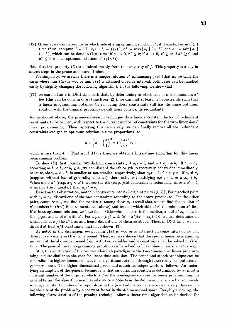
(f2) Given $x$ , we can determine in which side of $x$ an optimum solution $x$ “, if it exists, lies in $O(n)$

time (first, compute $I=\{i|a_{i}x+b_{i}=f(x)\},$ $a^{+}= \max\{a_{i}|i\in I\}$ and $a^{-}= \min\{a_{i}|$

$i\in I\}$ , which can be done in $O(n)$ time; if $a^{+}>0,$ $x^{*}\leq x$ ; if $a‘<0,$ $x^{*}\geq x$ ; if $a^{+}\geq 0$ and$a^{-}\leq 0,$ $x$ is an optimum solution; cf. (g1\sim 3)).

Note that this property (f2) is obtained mostly from the convexity of $f$ . This property is a key insearch steps in the prune-and-search technique.

For simplicity, we assume there is a unique solution $x$“ minimizing $f(x)$ (that is, we omit the

cases where $\min f(x)$ is $-\infty$ or $\min f(x)$ is attained on some interval; both cases can be handledeasily by slightly changing the following algorithm). In the following, we show that

(f3) we can find an $x$ in $O(n)$ time such that, by determining in which side of $x$ the minimum $x$“

lies (this can be done in $O(n)$ time from $(f2)$ ), we can find at least $n/4$ constraints such thata linear programming obtained by removing these constraints still has the same optimumsolution with the original problem (we call these constraints redundant).

As mentioned above, the prune-and-search techmique thus finds a constant factor of redundantconstraints, to be pruned, with respect to the current nunber of constraints for the two-dimensionallinear programming. Then, applying this recursively, we can finally remove all the redundantconstraints and get an optimum solution in time proportional to

$n+ \frac{3}{4}n+(\frac{3}{4})^{2}n+(\frac{3}{4})^{3}n+\cdots$

which is less than $4n$ . That is, if (f3) is true, we obtain a linear-time algorithm for this linearprogramming problem.

To show (f3), first consider two distinct constraints $y\geq a_{i}x+b_{i}$ and $y\geq a_{j}x+b_{j}$ . If $a_{i}=a_{j}$ ,according as $b_{i}<b_{j}$ or $b_{i}\geq b_{j}$ , we can discard the ith or $j$ th, respectively, constraint immediately,because, then, $a_{i}x+b_{i}$ is smaller or not smaller, respectively, than $a_{j}x+b_{j}$ for any $x$ . If $a_{\mathfrak{i}}\neq a_{j}$

(suppose without loss of generality $a_{i}>a_{j}$ ), there exists $x_{ij}$ satisfying $a_{l}x_{ij}+b_{i}=a_{j}x_{ij}+b_{j}$ .When $x_{ij}>x^{*}$ (resp. $x_{tj}<x^{*}$ ), we see the ith (resp. $jth$) constraint is redundant, since $a_{i}x^{*}+b_{i}$

is smaller (resp. greater) than $a_{j}x^{*}+b_{j}$ .Based on this observation, match $n$ constraints into $n/2$ disjoint pairs $\{(i,j)\}$ , For matched pairs

with $a_{i}=a_{j}$ , discard one of the two constraints according to the above procedure. For the otherpairs, compute $x_{ij}$ , and find the median $x’$ among those $x_{ij}$ (recall that we can find the median of$n’$ numbers in $O(n’)$ time as mentioned above) and test on which side of $x’$ the $minim\iota unx^{*}$ lies.If $x’$ is an optimum solution, we have done. Otherwise, since $x’$ is the median, a half of $x_{ij}’ s$ lies inthe opposite side of $x’$ with $x^{*}$ . For a pair $(i,j)$ with $(x’-x^{*})(x’-x_{ij})\leq 0$ , we can determine onwhich side of $x_{\mathfrak{i}j}$ the $x$

“ lies, and hence discard one of them as above. Thus, in $O(n)$ time, we candiscard at least $n/4$ constraints, and have shown (f3).

As noted in the discussion, even if $\min f(x)$ is $-\infty$ or is attained on some interval, we candetect it very easily in $O(n)$ time bound. Thus, we have shown that the special linear programmingproblem of the above-mentioned form with two variables and $n$ constraints can be solved in $O(n)$

time. The general linear programming problem can be solved in linear time in an analogous way.Still, this application of the prune-and-search paradigm to the two-dimensional linear program-

ming is quite similar to the case for linear-time selection. The prune-and-search technique can begeneralized to higher dimensions, and then algorithms obtained through it are really computational-geometric ones. The higher-dimensional prune-and-search technique works as follows. An under-lying assumption of the general technique is that an optimum solution is determined by at most aconstant number of the objects, which is $d$ in the nondegenerate case for linear progranuning. Ingeneral terms, the algorithm searches relative to $n$ objects in the d-dimensional space by recursivelysolving a constant number of sub-problems in the $(d-1)$-dimensional space recursively, thus reduc-ing the size of the problem by a constant factor in the d-dimensional space. Roughly speaking, thefollowing characteristics of the pruning technique allow a linear-time algorithm to be devised for

54

Figure 2.2. Linear $L_{1}$ approximation of points

a search relative to $n$ objects in the d-dimensional space. At each iteration, the algorithm prunesthe remaining objects by a constant factor, $\alpha$ , by applying a test a constant number of times. Thetest in the d-dimensional space is an essential feature of the algorithm since the complexity of thealgorithm depends on the test being able to report the relative position of an optimum solution inlinear time with respect to the number of remaining objects. The test in the d-dimensional spaceis performed by solving the $(d-1)$-dimensional subproblems as mentioned above. Hence, there area total of $O(\log n)$ steps, with the amount of time spent at each step geometrically decreasing asnoted above, taking linear time in total.

This approach was first adopted by Megiddo [22] et al. By this approach, linear programming ina fixed dimension can be solved in $o(2^{2^{d}})$ time, which is linear in $n$ . However, this time complexityis doubly exponential in $d$ , and the $algorit!un$ may be practical only for small $d$ . This complexity hasbeen improved in several ways (e.g., see [3]), but is still exponential with respect to $d$ . We will returnto this issue in the next section. Before it, we mention two applications of the prune-and-searchtechnique to larger special linear programming problems.

2.2 Applications of the prune-and-search paradigm to special linear program-ming problems

Here, we mention two applications of the prune-and-search paradigm to special linear programmingproblems which are not a two-dimensional linear programming problem. One is on linear $L_{1}$

approximation of $n$ points in the plane by Imai, Kato and Yamamoto [12] and the other is on theassignment problem with much fewer demand points than supply points by Tokuyama and Nakano[29].

(1) Linear $L_{1}$ approximation of pointsApproximating a set of $n$ points by a linear function, or a line in the plane, called the line-

fitting problem, is of fundamental importance in numerical computation and statistics. The mostfrequently used method is the least-squares method, but there are alternatives such as the $L_{1}$ andthe $L_{\infty}$ (or Chebyshev) approximation methods. Especially, the $L_{1}$ approximation is more robustagainst outliers than the least-squares method, and is preferable for noisy data.

Let $S$ be a set of $n$ points $p_{i}$ in the plane and denote the $(x, y)$-coordinate of point $p_{i}$ by$(x_{i}, y;)(i=1, \ldots,n)$ . For an approximate line defined by $y=ax+b$ with parameters $a$ and $b$ ,the following error criterion, minimizing the $L_{1}$ norm, of the approximate line to the point set $S$

defines the $L_{1}$ approximation:

$\min_{a,b}\sum_{i=1}^{n}|y_{i}-(ax_{i}+b)|$

Figure 2.2 depicts the case of $n=10$ with an outlier.

55

This problem can be formulated as the following linear programming problem with $n+2$ variables$a,$ $b,$ $c_{i}(i=1, \ldots, n)$ :

$\min$ $\sum_{i=1}^{n}c_{i}$

s.t. $y_{i}-(ax_{i}+b)\leq c_{i}$

$-y_{i}+(ax_{i}+b)\leq c_{i}$

Here, $x,,$ $y_{i}$ $(i=1, \ldots , n)$ are given constants. This linear programming problem has $n+2$variables and more inequalities, and hence the linear-time algorithm for linear programming in afixed dimension cannot be applied. However, the problem is essentially a two-dimensional problem.By using the point-line duality transformation, which is one of the best tools used in computationalgeometry, we can transform this problem so that the two-diinensional prune-and-search techniquemay be applied. In the $L_{1}$ approximation problem, however, any infinitesimal movement of anypoint in $S$ changes the norm (and possibly the solution), and, in that sense, redundant points withrespect to an optimum solution do not exist. Hence, direct application of the pruning techniquedoes not produce a linear-time algorithm.

Imai, Kato and Yamamoto [12] give a method of overcoming this difficulty by making fulluse of the piecewise linearity of the $L_{1}$ norm to obtain a linear-time algorithm. Furthennore, inhis master’s thesis, Kato generalizes this result to higher dimensional $L_{I}$ approximation problem.Although these algorithms are a little complicated, they reveal how powerful the prune-and-searchteclmique is in purely computational-geometric settings.

(2) Assignment problemThe assignment problem is a typical problem in network flow. The assignment problem with $n$

supply vertices and fewer $k$ demand vertices is formulated as follows:

$\min$ $\sum_{i=1j}^{n}\sum_{=1}^{k}w_{ij^{X}ij}$

$s.t$ . $\sum_{i=1}^{n}x_{ij}=n_{j}$ $(j=1, \ldots, k)$ , $\sum_{i=1}^{k}x_{ij}=1$ $(i=1, \ldots, r\iota)$

$0\leq x_{ij}\leq 1$

where $x_{ij}$ are variables and $\sum_{j=1}^{k}n_{j}=n$ for positive integers $n_{j}$ . Since this is an assignmentproblem, $x_{1i}$ should be an integer, but all the extreme points of the polytope of this problem areinteger-valued and hence this problem can be formulated as a simple linear programnuing problemof $kn$ variables.

For this assignment problem, Tokuyama and Nakano [29] give the following nice geometriccharacterization. For this assignment problem, consider a set $S$ of $n$ points $p$; in the k-dimensionalspace whose coordinates are defined by

$p:=(w_{i1}, w_{i2}, \ldots,w_{ik})-\frac{1}{k}\sum_{j=1}^{k}w_{ij}(1,1, \ldots, 1)$ .

Each point in $S$ is on the hyperplane $H:x_{1}+x_{2}+\cdots+x_{k}=0$ . For a point $g=(g_{1},g_{2}, \ldots, g_{k})$ onthe hyperplane $H$ , define

$T(g;j)= \bigcap_{h=I}^{k}$ { $(x_{1},$$\ldots,$

$x_{k})$ on the hyperplane $H|x_{j}-x_{h}\leq g_{j}-g_{h}$ }

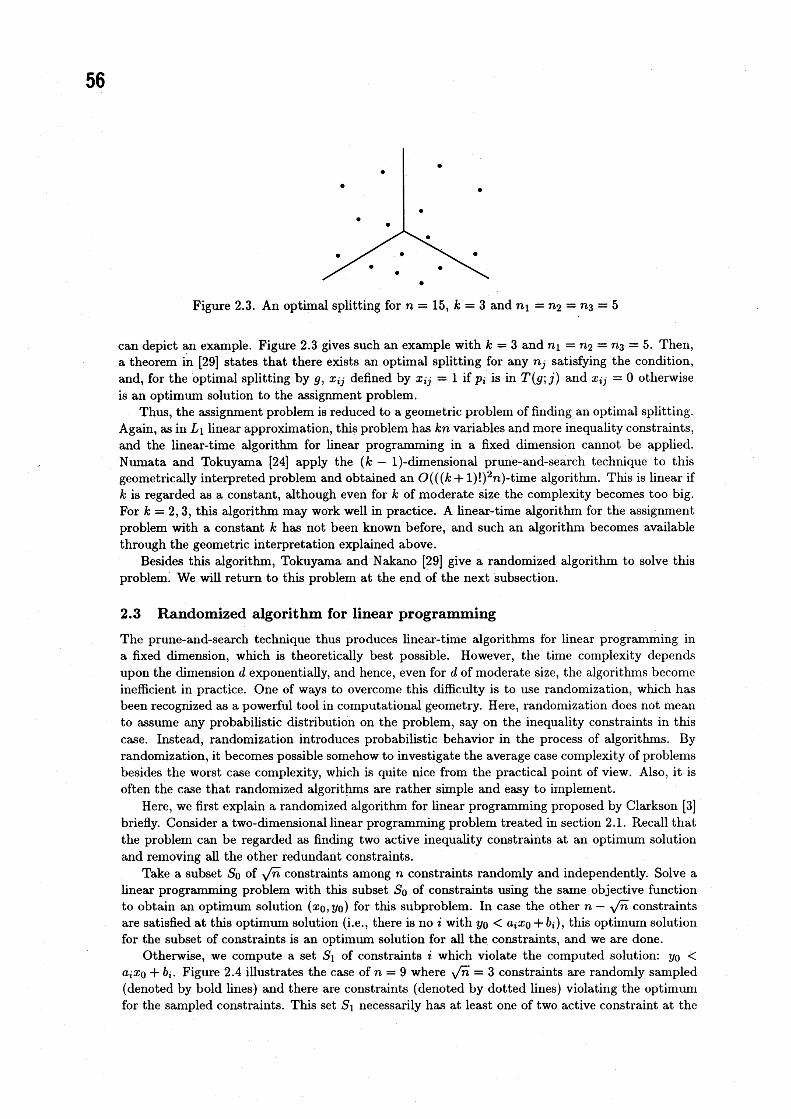
$T(g;j)(j=1, \ldots, k)$ partition the hyperplane $H$ . This partition is called an optimal splitting ifeach $T(g;j)$ contains $n_{j}$ points from $S$ . In the case of $k=3$ , the hyperplane is just a plane, and we

56

Figure 2.3. An optinal splitting for $n=15,$ $k=3$ and $n_{1}=n_{2}=n_{3}=5$

can depict an example. Figure 2.3 gives such an example with $k=3$ and $n_{1}=n_{2}=n_{3}=5$ . Then,a theorem in [29] states that there exists an optimal splitting for any $n_{j}$ satisfying the condition,and, for the optimal splitting by $g,$ $x_{ij}$ defined by $x_{ij}=1$ if $p_{i}$ is in $T(g;j)$ and $x_{ij}=0$ otherwiseis an optimum solution to the assignment problem.

Thus, the assignment problem is reduced to a geometric problem of finding an optimal splitting.Again, as in $L_{I}$ linear approximation, this problem has $kn$ variables and more inequality constraints,and the linear-time algorithm for linear programming in a fixed dimension cannot be applied.Numata and Tokuyama [24] apply the $(k-1)$-dimensional prune-and-search technique to thisgeometrically interpreted problem and obtained an $O(((k+1)!)^{2}n)$-time algorithm. This is linear if$k$ is regarded as a constant, although even for $k$ of moderate size the complexity becomes too big.For $k=2,3$ , this algoritin may work well in practice. A linear-time algorithm for the assignmentproblem with a constant $k$ has not been known before, and such an algorithm becomes availablethrough the geometric interpretation explained above.

Besides this algorithm, Tokuyama and Nakano [29] give a randomized algorithm to solve thisproblem. We will return to this problem at the end of the next subsection.

2.3 Randomized algorithm for linear programming

The prune-and-search technique thus produces linear-time algorithms for linear programming ina fixed dimension, which is theoretically best possible. However, the time complexity dependsupon the dimension $d$ exponentially, and hence, even for $d$ of moderate size, the algorit!uns becomeinefficient in practice. One of ways to overcome this difficulty is to use randomization, which hasbeen recognized as a powerful tool in computational geometry. Here, randomization does not meanto assume any probabilistic distribution on the problem, say on the inequality constraints in thiscase. Instead, randomization introduces probabilistic behavior in the process of algorithms. Byrandomization, it becomes possible somehow to investigate the average case complexity of problemsbesides the worst case complexity, which is quite nice from the practical point of view. Also, it isoften the case that randomized algorithms are rather simple and easy to implement.

Here, we first explain a randomized algorithm for linear programming proposed by Clarkson [3]briefly. Consider a two-dimensional linear programming problem treated in section 2.1. Recall thatthe problem can be regarded as finding two active inequality constraints at an optimum solutionand removing all the other redundant constraints.

Take a subset $S_{0}$ of $\sqrt{n}$ constraints among $n$ constraints randomly and independently. Solve alinear programming problem with this subset $S_{0}$ of constraints using the same objective functionto obtain an optimum solution $(x_{0},y_{0})$ for this subproblem. In case the other $n-\sqrt{n}$ constraintsare satisfied at this optimum solution (i.e., there is no $i$ with $y_{0}<a_{i}x_{0}+b_{\mathfrak{i}}$ ), this optimum solutionfor the subset of constraints is an optimum solution for all the constraints, and we are done.

Otherwise, we compute a set $S_{1}$ of constraints $i$ which violate the computed solution: $y_{0}<$

$a_{i}x_{0}+b_{i}$ . Figure 2.4 illustrates the case of $n=9$ where $\sqrt{n}=3$ constraints are randomly sampled(denoted by bold lines) and there are constraints (denoted by dotted lines) violating the optimuunfor the sampled constraints. This set $S_{I}$ necessarily has at least one of two active constraint at the

57

Figure 2.4. A randomized algorithm for linear programming

global optimuun solution, which may be observed by overlaying the two active constraints formingthe optimum with the current subset of constraints. In Figure 2.4, exactly one constraint activeat the global optimum is included in $S_{1}$ . The size of $S_{1}$ depends on the subset of $\sqrt{n}$ constraintschosen through randomization. It can be shown that the expected size of $S_{1}$ is $o(\Gamma^{n})$ , which is akey of this randomized algorithm. That is, by randomly sampling a subset $S_{0}$ of $\sqrt{n}$ constraints,we can find a set $S_{1}$ of constraints of expected size $O(\Gamma n)$ which contains at least one of activeconstraints at the global optimum solution.

We again sample another set $S_{2}$ of $\sqrt{n}$ constraints, and this time solve a linear programmingproblem with constraints in $S_{1}\cup S_{2}$ . Let $S_{3}$ be a set of constraints violating the optimuin solutionto the subproblem for $S_{1}\cup S_{2}$ . Again, it can be seen that the expected size of $S_{3}$ is $O(\sqrt{n})$

and that $S_{1}\cup S_{3}$ contains at least two among two active constraints (hence, exactly two in thistwo-dimensional case) at the global optimum solution. Since $S_{1}\cup S_{3}$ contains those two activeconstraints at the optimum solution and its size is $O(\sqrt{}\overline{n})$ on the average, the original problemfor $n$ constraints is now reduced to that for $o(\Gamma^{n})$ constraints. Then, recursively applying thisprocedure solves the problem efficiently.

Based on the idea outlined above, Clarkson [3] $gives\ovalbox{\tt\small REJECT}$ Las Vegas algorithm which solves thelinear programuning problem in a fixed dimension $d$ rigorously in $O(d^{2}n+t(d)\log n)$ running timewith high probability close to 1, where $t(d)$ is a function of $d$ and is exponential in $d$ . By random-ization, the constant factor of $n$ becomes dependent on $d$ only polynomially, unlike the linear-timealgorithm based on the prune-and-search paradigm. This is achieved by using random sampling inthe algorithm. However, still there is a term in the complexity function which is exponential in $d$ ,and the algorithm is not a strongly polynomial algorithm.

A main issue in the design and analysis of this randomized algorithm is to evaluate the expectednumber of violating constraints to the optimum for the sampled set $S_{0}$ . In this case, this evaluationcan be performed completely in a discrete way. However, in more general case, the continuousmodel of probability may be used as in $[9, 31]$ , and, in this sense, introducing randomization ingeometric algorithms may lead to investigating continuous structures of geometric problems more.

Now, return to the assigmnent problem with $k$ demand vertices and $n$ supply vertices mentionedin the previous subsection. The prune-and-search paradigm yields the $O((k+1)!)^{2}n)$-time algorithmfor it as mentioned above. Tokuyama and Nakano [29] propose a randomized algorithm, makinguse of random sampling, with randomized time complexity $O(kn+k^{3.5}n^{0.5}\log n)$ . This algorithmis optimum for $k\ll n$ , since the complexity becomes simply $O(kn)$ then. Thus, for the assignmentproblem with $k\ll n$ , randomization gives a drastic result. lt should be emphasized again that thisbecomes possible by establishing a nice bridge between geometry and combinatorial optimization,and by applying the randomization paradigm suitable for geometric problems.

These randomized algorithms are regarded as fruitful results by combining computational geo-

58

metric results with linear progranuning and its special case. We will return to this issue in section 4after explaining a continuous approach.

3 Linear Programming in Mathematical Programming

For linear programming, a nonlinear approach has recently been shown to be efficient for large-scale linear programming problems in mathematical programming, and the so-called interior-pointmethod is now recognized as a powerful method for linear programming. In this section, amongmany interior-point algorithms, we explain the multiplicative penalty function method proposedby Iri and Imai [15]. $Tl_{1}en$ , we show that, by applying the general interior-point method, animproved algoritin may be obtained for the planar minimum-cost flow problem, which is $a\dot{s}pecial$

case of linear programming. This is another kind of merit of the interior-point method for linearprogramming. Applying the interior-point method to constructing parallel algorithms for linearprogramming is also discussed.

3.1 Multiplicative penalty function method for linear programming

The multiplicative penalty fumction method, proposed by Iri and Imai [15], is an interior methodwhich minimizes the convex multiplicative penalty function defined for a given linear programmingproblem with inequality constraints by the Newton method. In this sense, the multiplicative penaltyfunction method can be said to be the simplest and most natural method among interior-pointmethods using penalty functions. The multiplicative penalty function may be viewed as a affinevariant of the potential function of Karmarkar [16]. $\ln[15]$ , the local quadratic convergence ofthe method was shown, while the global convergence property was left open. Zhang and Shi [32]prove the global linear convergence of the method under an assumption that the line search canbe performed rigorously. Imai [11] shows that the number of main iterations in the multiplicativepenalty function method is $O(n^{2}L)$ , where at each iteration a main task is to solve a linear systemof equations of $d$ variables to find the Newton direction. Iri [14] further shows that the originalversion of the multiplicative penalty function method runs in $O(n^{1.5}L)$ main iterations and thatan algorithm with an increased penalty parameter runs in $O(nL)$ iterations. In that paper [14], itis also shown that the convex quadratic programnung problem can be solved by the multiplicativepenalty function method within the same complexity.

There are now many interior-point algorithms for linear programming. For those algorithms,the interested readers may refer to [16, 19, 23].

We consider the following linear programming problem in the form mentioned in the introduc-tion. In the sequel, we further assume the following (cf. [15]):(1) The feasible region $X=\{x|Ax\geq b\}$ is bounded.(2) The interior Int $X$ of the feasible region $X$ is not empty.(3) The minimum value of $c^{T}x$ is zero.The assumption (3) might seem to be a strong one, but there are several techniques to make thisassumption hold for a given problem. Then the multiplicative penalty function for this linearprogrammming problem is defined as follows:

$F(x)=( c^{T}x)^{n+\delta}/\prod_{i=1}^{n}(a_{i}^{T}x-b_{i})$ $(x\in IntX)$

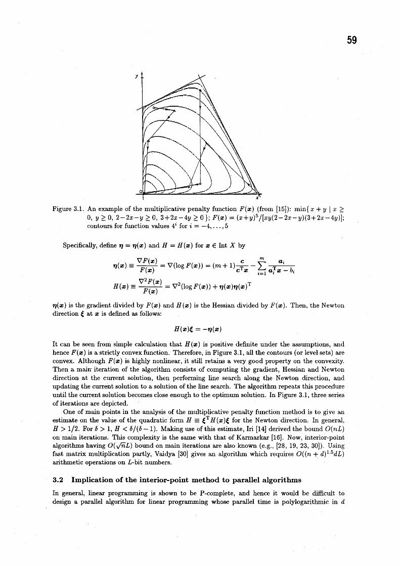
where $a_{1}^{T}\in R^{d}$ is the i-th row vector of $A$ and $\delta$ is a constant greater than or equal to 1. Thisfunction is introduced in [15], and there $\delta$ is set to one. In [14], $\delta$ is set to approximately $n$ . InFigure 3.1, contours of $F(x)$ in the two-dimensional case with $n=4$ are shown. Under theseassumptions, when $F(x)arrow 0$, the distance between $x$ and the set of optimum solutions convergesto zero. The multiplicative penalty function method directly minimizes the penalty function $F(x)$

by the Newton method, starting from some initial interior point.

59

Figure 3.1. An example of the multiplicative penalty function $F(x)$ (from [15]): $\min\{x+y|x\geq$$0,$ $y\geq 0,2-2x-y\geq 0,3+2x-4y\geq 0$ } $;F(x)=(x+y)^{5}/[xy(2-2x-y)(3+2x-4y)]$ ;contours for function values $4^{i}$ for $i=-4,$ $\ldots,$

$5$

Specifically, define $\eta=\eta(x)$ and $H=H(x)$ for $x\in IntX$ by

$\eta(x)\equiv\frac{\nabla F(x)}{F(x)}=\nabla(\log F(x))=(m+1)\frac{c}{c^{T_{X}}}-\sum_{i=1}^{m}\frac{a_{i}}{a_{i}^{T}x-b_{i}}$

$H(x) \equiv\frac{\nabla^{2}F(x)}{F(x)}=\nabla^{2}(\log F(x))+\eta(x)\eta(x)^{T}$

$\eta(x)$ is the gradient divided by $F(x)$ and $H(x)$ is the Hessian divided by $F(x)$ . Then, the Newtondirection $\xi$ at $x$ is defined as follows:

$H(x)\xi=-\eta(x)$

It can be seen from simple calculation that $H(x)$ is positive definite under the assumptions, andhence $F(x)$ is a strictly convex function. Therefore, in Figure 3.1, all the contours (or level sets) areconvex. Although $F(x)$ is highly nonlinear, it still retains a very good property on the convexity.Then a main$\cdot$ iteration of the algoritIun consists of computing the gradient, Hessian and Newtondirection at the current solution, then performing line search along the Newton direction, andupdating the current solution to a solution of the line search. The algorithm repeats this procedureuntil the current solution becomes close enough to the optimum solution. In Figure 3.1, three seriesof iterations are depicted.

One of main points in the analysis of the multiplicative penalty function method is to give anestimate on the value of the quadratic form $H\equiv\xi^{T}H(x)\xi$ for the Newton direction. In general,$H>1/2$ . For $\delta>1,$ $H<\delta/(\delta-1)$ . Making use of this estimate, Iri [14] deriyed the bound $O(nL)$

on main iterations. This complexity is the same with that of Karmarkar [16]. Now, interior-pointalgorithms having $O(\sqrt{n}L)$ bound on main iterations are also known (e.g., [28, 19, 23, 30]). Usingfast matrix multiplication partly, Vaidya [30] gives an algorithm which requires $O((n+d)^{1.5}dL)$

arithmetic operations on L-bit numbers.

3.2 Implication of the interior-point method to parallel algorithms

In general, linear programmuing is shown to be P-complete, and hence it would be difficult todesign a parallel algorithm for linear programming whose parallel time is polylogarithmic in $d$

60

and $n$ . However, the interior-point method may be used to devise parallel algorithms whose timecomplexity is sublinear in $d$ and $n$ . This is also the case for linear programming problems arisingin geometric situations.

In the interior-point method, each iteration itself can be highly parallelized. In fact, as men-tioned repeatedly, a main step of the iteration is to solve the linear system of equations, which canbe parallelized very efficiently in polylogarithmic time in theory (e.g., see [26]).

This implies that, applying interior-point algorithms requiring $O(\sqrt{n}L)$ main iterations to alinear programming problem, a parallel algorithm for the problem with $O$ ( $\sqrt{n}L$ polylog n) paralleltime complexity can be obtained. This parallel time is sublinear in $n$ , although it is linear in $L$ .For some network flow problem whose constraint matrix is totally unimodular and whose costs andcapacities are constants, $L$ can be considered to be a constant, and hence this approach gives atotally sublinear parallel $algorit!un$ for it. Even if $L$ is not a constant, parallel algorithms whosecomplexity is sublinear in $n$ are of great interest. This approach is adopted in [8].

Considering the application of the interior-point method to planar network flow, which willbe explained in the next subsection, the nested dissection technique can also be parallelized [26],and a parallel algorithm with $O(\sqrt{n}\log^{3}n\log(n\gamma))$ parallel time using $O(n^{I.094})$ processors can beobtained [13], where $\gamma$ is the largest absolute value among edges costs and capacities represented byintegers. Also, this parallel algorithm is best possible with respect to the sequential algorithm, tobe mentioned in the next subsection, that is, the parallel time complexity multiplied by the numberof processors is within a polylog factor of the sequential time complexity. This result roughly saysthat the planar minimuun cost flow problem can be solved in parallel in $O(n^{0.5+\epsilon})$ time with almostlinear number of processors, which is currently best possible.

Thus, treating a special linear programming problem in a more general setting, better parallelalgorithms may be obtained. Here, it may be said that the continuous approach makes this possible.

3.3 Applying the interior-point method for planar minimum cost flow

The interior-point method can be used to derive a new algorithm having the best time $(()111\})lcxity$

to some special linear progranuning problems $[13, 30]$ . In $t1_{1}is$ section we describe all applicatiou ofthe interior-point method to the planar minimum cost flow problem given by Imai and Iwano [13].Also, some results of preliminary computational experiments are shown.

In these years, much research has been done on the minimum cost flow problem on networks.The minimum cost flow problem is the most general problem in network flow theory that admitsstrongly polynomial algorithms. Recently, the interior point method for linear programming hasbeen applied to the minimum cost flow problem, which is a very special case of linear programming,by Vaidya [30] from the viewpoint of sequential algorithms and by Goldberg, Plotkin, Shmoysand Tardos [8] from the viewpoint of parallel algorithms. For the planar minimum cost flowproblem, the best strongly polynomial time algorithm is given by Orlin [25], and has complexity of$O(m(m+n\log n)\log n)$ for networks with $m$ edges and $n$ vertices.

If we restrict networks, the efficiency of the interior-point method may be further enhanced.Here, we consider the minimum cost flow problem on networks having good separators, that is,s(n)-separable networks. Roughly, an s(n)-separable graph of $n$ vertices can be divided into twosubgraphs by removing $s(n)$ vertices such that there is no edge between the two subgraphs and thenumber of vertices in each subgraph is at most $\alpha n$ for a fixed constant $\alpha<1$ . A planar grid graphis easily seen to be $\sqrt{n}$-separable [7]. General planar graphs are $O(\sqrt n\urcorner$-separable, which is wellknown as the planar separator theorem by Lipton and Tarjan [21].

For a system of linear equations $\tilde{A}\tilde{x}=\sim b$ with $n\cross n$ symmetric matrix $\tilde{A}$ , if the nonzero patternof $\tilde{A}$ corresponds to that of the adjacency matrix of an s(n)-separable graph, the system $A\tilde{x}=\sim b$

can be solved more efficiently than general linear systems. This is originally shown for planar gridgraphs by George [7], and the technique is called nested dissection. The technique is generalizedto s(n)-separable graphs by Lipton, Rose and Tarjan [20]. For $A$ corresponding to a planar graph,the system can be solved in $O(n^{1.I88})$ time and $O(n\log n)$ space by further making use of the fast

$6t$

Table 3.1. Preliminary computational results for the minimum cost flow problem on $k\cross k$ gridnetwork

matrix multiplication by Coppersmith and Winograd [4].When applying the interior method, a main step is to solve a linear system of equation to

compute a search direction such as the Newton direction as mentioned above. In solving the linearsystem $\tilde{A}\tilde{x}=b\sim$ for the linear programming problem of the form mentioned in the beginning of theintroduction, we mainly have to solve a linear system with a $d\cross d$ symmetric matrix $\tilde{A}$ defined by

$\tilde{A}=A^{T}DA$

where $D$ is a diagonal matrix whose diagonal elements are positive. For most interior-point methodsproposed so far, their search direction can be computed relatively easily if the linear system for this$\tilde{A}$ is solvable by some efficient method.

In the case of network flow, the main part of the matrix $A$ is the incidence matrix of underlyinggraph. Suppose $A$ is exactly the incidence matrix. For this $A$ , the nonzero pattem of $\tilde{A}=A^{T}DA$

exactly corresponds to the nonzero pattem of the adjacency matrix of the same graph.Therefore, when the network is an s(n)-separable graph, the technique of nested dissection can

be applied in the main step of the interior-point method. By elaborating this combination of theinterior-point method with restart procedure by Vaidya [30] and the nested dissection technique inmore detail, for the planar minimum cost flow problem, $O(n^{1.594}\vee\Gamma og\overline{n}\log(n\gamma))$ time and $O(n\log n)$

space [13], where $\gamma$ is the largest absolute value among edges costs and capacities represented byintegers. Parallel results corresponding to this is mentioned at the end of the preceding subsection.

When $\gamma$ is polynomially bounded in $n$ , the sequential time complexity becomes $O(n^{I.6})$ which isbest among existing algorithuns by a factor roughly $O(n^{0.4})$ . These results can be generalized to theminimum cost flow problem on s(n)-separable networks such as three-dimensional grid networks.Also, in computational geometry, there arise linear progranuning problems having special structures(e.g., [10]) which may be used to enhance the efficiency in solving the linear system.

In concluding this subsection, we show results of a computational experiment of using the nesteddissection technique to the minimum cost flow problem on grid networks. In this experiment, asan interior-point method, the affine-scaling method, which would be the simplest interior-method,is used, and at each iteration the linear system is solved by the nested dissection technique. Table3.1 gives the results. Also, to compare its result withe some other method, the running time ofthe network simplex code, taken from a book [17], is also shown. In the simplex method, oneiteration corresponds to one pivoting. It should be noted that, in comparing these two methods,simply comparing the running times listed here is meaningless, since these two methods use differentstopping criteria and both implementations are not best possible at all. Instead, in the table, itshould be observed how the running times of both methods increase as the size of networks increases.

62

From this table, it is seen that running times of the affine-scaling interior method increasesmore slowly than that for the network simplex method. This indicates that as the size of linearprogramming becomes large, the interior-point method becomes relatively more efficient than thesimplex method in this case. It is now widely recognized that this tendency mostly holds for generalcases.

4 Combining Techniques in Computational Geometry and Math-ematical Programming

At the end of section 2, we have seen how some of computation geometric technique can be coInbinedwith pure linear programming theory through randomization. In this section, we mention a resultby Adler and Shamir [1] which combines a randomized algorithm with an interior-point method.This is really a nice example of combining results in computational geometry and mathematicalprogramming.

The algorithm is basically similar to Clarkson’s randomized algorithm [3]. Instead of simpleuniform random sampling, it uses self-adjusting weighted random sampling and tries to keep thenumber of sampled constraints smaller with respect to $d$ . That is, instead of maintaining all theviolating constraints in the Clarkson’s algorithm, this algorithm increases, for each violating con-straint, the probability for the constraint to be sampled in later steps. By this strategy, throughoutthe algorithm, it simply samples $O(d^{2})$ constraints, not $\Gamma n$ constraints at each stage.

In the original randomized algorithm, a subproblem is solved recursively by the same randomizedalgorithm until the size of the subproblem becomes some constant. Instead, any interior-pointmethod may be used to solve the subproblem. Since the size of this subproblem is relativelysmaller than the whole size (in fact, the nuunber of constraints in subproblems in the process of thisalgorithm is bounded by $O(d^{2})$ with $d$ variables as mentioned above), the randomized algorithmmay gain some merit from this. We skip the details and just mention final results in [1]. Based onthe strategy mentioned above, it can be shown that the linear programming problem is solvable inexpected time $O((nd+d^{4}L)d\log n)$ . This improves much the time complexity if $d\ll n$ , which isquite interesting from the viewpoint of the interior-point method.

This way of combining the interior-point method with a certain computational-geometric tech-nique is still na’ive. Besides this algorithm, randomization would be useful in some parts of theinterior-point method, and research along this line, combining the continuous approach and discreteapproach, would deserve much attention.

5 Concluding Remarks

We have discussed about linear programming from the standpoints of both computational geometryand mathematical programming, and have explain some fruitful results obtained through combiningthe idea in both fields.

In the introduction, both of discrete and continuous aspects of linear programming are men-tioned. Since discrete structures are easier to handle by computers, theoretical computer sciencehas so far pursued discrete side very much. In recent years, there have been proposed many non-linear approach to discrete optimization problems. As in linear programming, handing nonlinearphenomena in the theory of discrete algorithms and complexity will be required in future. Evenin the low dimensional space treated in computational geometry, we have not yet fully understoodhow to treat the continuous world in a discrete setting, and this type of new problems will deservefurther investigation.

63

References

[1] I. Adler and R. Shamir: A Randomization Scheme for Speeding Up Algorithms for LinearProgramming Problems with High Constraints-to-Variables Ratio. DIMA CS Technical Report89-7, DIMACS, 1989.

[2] M. Blum, R. W. Floyd, V. Pratt, R. L. Rivest and R. E. Tarjan: Time Bounds for Selection.Joumal of Computer and System Sciences, Vol.7 (1973), pp.448-461.

[3] K. L. Clarkson: A Las Vegas Algorithm for Linear Programming when the Dimension is Small.Proceedings of the 29th IEEE Annual Symposium on Foundations of Computer Science, 1988,pp.452-456.

[4] D. Coppersmith and S. Winograd: Matrix Multiplication via Arithunetic Progressions. Journalof Symbolic Computation, Vol.9, No.3 (1990), pp.251-280.

[5] G. Dantzig: Linear Programming and Extensions. Princeton University Press, 1963.

[6] M. R. Garey and D. S. Johnson: Computers and Intractability: A Guide to the Theory ofNP-Completeness. W. H. Freeman, San Francisco, 1979.

[7] A. George: Nested Dissection of a Regular Finite Element Mesh. SIAM Journal on NumericalAnalysis, Vol.10, No.2 (1973), pp.345-363.

[8] A. V. Goldberg, S. A. Plotkin, D. B. Shmoys and \’E. Tardos: Interior-Point Methods in ParallelComputation. Proceedings of the 30th Annual IEEE Symposium on Foundations of ComputerScience, 1989, pp.350-355.

[9] D. Haussler and E. Welzel: Epsilon-Nets and Simplex Range Queries. Proceesings of the 2ndAnnual ACM Symposium on Computational Geometry, 1986, pp.61-71.

[10] H. Imai: A Geometric Fitting Problem of Two Corresponding Sets of Points on a Line. IE-ICE Transactions on Fundamentals of Electronics, Communications and Computer Sciences,Vol.E74, No.4 (1991), pp.665-668.

[11] H. Imai: On the Polynomiality of the Multiplicative Penalty Function Method for LinearProgramming and Related Inscribed Ellipsoids. IEICE Transactions on Fundamentals of Elec-tronics, Communications and Computer Sciences, Vol.E74, No.4 (1991), pp.669-671.

[12] H. Imai, K. Kato and P. Yamamoto: A Linear-Time Algorithm for Linear $L_{1}$ Approximationof Points. Algorithmica, Vol.4, No.1 (1989), pp.77-96.

[13] H. Imai and K. Iwano: Efficient Sequential and Parallel Algorithms for Planar Minium CostFlow. Proceedings of the SIGAL International Symposium on Algorithms (T. Asano, T. Ibaraki,H. Imai, T. Nishizeki, eds.), Lecture Notes in Computer Science, Vol.450, Springer-Verlag,Heidelberg, 1990, pp.21-30.

[14] M. Iri: A Proof of the Polynomiality of the Iri-Imai Method. Manuscript, to be presented atthe 14th International Symposiuun on Mathematical Programning, 1991.

[15] M. Iri and H. Imai: A Multiplicative Barrier Function Method for Linear Programming. Al-gorithmica, Vol.1 (1986), pp.455-482.

[16] N. Karmarkar: A New Polynomial-Time Algorithm for Linear Programming. Combinatorica,Vol.4 (1984), pp.373-395.

[17] J. L. Kennington and R. V. Helgason: Algorithms for Network Programming. John Wiley &Sons, New York, 1980.

64

[18] L. G. Khachian: Polynomial Algoritlmls in Linear Programming. Zh. Vychisl. Mat. i Mat.Fiz., Vol.20 (1980), pp.51-68 (in Russian); English translation in U.S.S. R. Comput. Math.and Math. Phys., Vol.20 (1980), pp.53-72.

[19] M. Kojima, S. Mizuno and A. Yoshise: A Polynomial-Time Algorithm for a Class of LinearComplementary Problems. Mathematical Programming, Vol.44 (1989), pp.1-26.

[20] R. J. Lipton, D. J. Rose, and R. E. Tarjan: Generalized Nested Dissection. SIAM Journal onNumerical Analysis, Vol.16, No.2 (1979), pp.346-358.

[21] R. J. Lipton and R. E. Tarjan: A Separator Theorem for Planar Graphs. SIAM Journal onApphed Mathematics, Vol.36, No.2 (1979), pp.177-189.

[22] N. Megiddo: Linear Programming in Linear Time when the Dimension is Fixed. Journal ofthe Association for Computing Machinery, Vol.31 (1984), pp.114-127.

[23] R. C. Monteiro and I. Adler: Interior Path Following Primal-Dual Algorithms Part II: ConvexQuadratic Programming. Mathematical Programming, Vo..44 (1989), pp.43-66.

[24] K. Numata and T. Tokuyama: Splitting a Configuration in a Simplex. Proceedings of theSIGAL International Symposium on $Algo\sqrt thms$ (T. Asano, T. Ibaraki, H. Imai, T. Nishizeki,eds.), Lecture Notes in Computer Science, Vol.450, Springer-Verlag, Heidelberg, 1990, pp.429-438.

[25] J. B. Orlin: A Faster Strongly Polynomial Minimum Cost Flow Algorithm. Proceedings of the20th Annual A CM Symposium on Theory of Computing, 1988, pp.377-387.

[26] V. Pan and J. Reif: Efficient Parallel Solution of Linear Systems. Proceedings of the 17thAnnual ACM Symposium on Theory of $Compui\{ng$ , Providence, 1985, pp.143-152.

[27] F. Preparata and M. I. Shamos: Computational Geometry: An Introduction. Springer-Verlag,New York, 1985.

[28] J. Renegar: A Polynomial-Time Algorithm, based on Newton’s Method, for Linear Program-ming. Mathematical Programming, Vol.40 (1988), pp.59-93.

[29] T. Tokuyama and J. Nakano: Geometric Algorithuns for a Minimum Cost Assigmnent Problem.Proceedings of the 7th Annual ACM Symposium on Computational Geometry, 1991, pp.262-271.

[30] P. Vaidya: Speeding-Up Linear Programming Using Fast Matrix Multiplication. Proceeding ofthe 30th Annual IEEE Symposium on Foundations of Computer Science, 1989, pp.332-337.

[31] V. N. Vapnik and A. Ya. Chervon\’enkis: On the Uniforn Convergence of Relative Frequencies ofEvents to Their Probabilities. Theory of Probability and Its Applications, Vol.16, No.2 (1971),pp.264-280.

[32] S. Zhang and M. Shi: On Polynomial Property of Iri-Imai’s New AlgoritIun for Linear Pro-gramming. Manuscript, 1988.